Embed Size (px)
Citation preview
UC-Net: Uncertainty Inspired RGB-D Saliency Detection
via Conditional Variational Autoencoders
Jing Zhang1,4,5 Deng-Ping Fan2,6,∗ Yuchao Dai3
Saeed Anwar1,5
Fatemeh Sadat Saleh1,4 Tong Zhang1 Nick Barnes1
1 Australian National University 2 CS, Nankai University 3 Northwestern Polytechnical University4 ACRV 5 Data61 6 Inception Institute of Artificial Intelligence (IIAI), Abu Dhabi, UAE
Abstract
In this paper, we propose the first framework (UC-
Net) to employ uncertainty for RGB-D saliency detection
by learning from the data labeling process. Existing RGB-
D saliency detection methods treat the saliency detection
task as a point estimation problem, and produce a single
saliency map following a deterministic learning pipeline.
Inspired by the saliency data labeling process, we propose
probabilistic RGB-D saliency detection network via condi-
tional variational autoencoders to model human annota-
tion uncertainty and generate multiple saliency maps for
each input image by sampling in the latent space. With the
proposed saliency consensus process, we are able to gener-
ate an accurate saliency map based on these multiple pre-
dictions. Quantitative and qualitative evaluations on six
challenging benchmark datasets against 18 competing al-
gorithms demonstrate the effectiveness of our approach in
learning the distribution of saliency maps, leading to a new
state-of-the-art in RGB-D saliency detection1.
1. Introduction
Object-level visual saliency detection involves separat-
ing the most conspicuous objects that attract humans from
the background [27, 2, 55, 63, 38, 29, 62]. Recently, vi-
sual saliency detection from RGB-D images have attracted
lots of interest due to the importance of depth information
in human vision system and the popularity of depth sensing
technologies [61, 64]. Given a pair of RGB-D images, the
task of RGB-D saliency detection aims to predict a saliency
map by exploring the complementary information between
color image and depth data.
The de-facto standard for RGB-D saliency detection is
to train a deep neural network using ground truth (GT)
∗Corresponding author: Deng-Ping Fan ([email protected])1Our code is publicly available at: https://github.com/
JingZhang617/UCNet.
Image Depth GT Ours (1) Ours (2)
Figure 1. Provided GT compared with UC-Net (ours) predicted
saliency maps. For images with a single salient object (1 st row),
we can produce consistent prediction. When multiple salient ob-
jects exist (2nd row), we can produce diverse predictions.
saliency maps provided by the corresponding benchmark
datasets, where the GT saliency maps are obtained through
human consensus or by the dataset creators [18]. Building
upon large scale RGB-D datasets, deep convolutional neural
network based models [21, 61, 6, 24] have made profound
progress in learning the mapping from an RGB-D image
pair to the corresponding GT saliency map. Considering the
progress for RGB-D saliency detection under this pipeline,
in this paper, we would like to argue that this pipeline fails
to capture the uncertainty in labeling the GT saliency maps.
According to research in human visual perception [33],
visual saliency detection is subjective to some extent. Each
person could have specific preferences in labeling the
saliency map (which has been previous discussed in user-
specific saliency detection [26]). Existing approaches to
RGB-D saliency detection treat saliency detection as a point
estimation problem, and produce a single saliency map for
each input image pair following a deterministic learning
pipeline, which fails to capture the stochastic characteris-
tic of saliency, and may lead to a partisan saliency model as
shown in second row of Fig. 1. Instead of obtaining only
a single saliency prediction (point estimation), we are in-
terested in how the network produces multiple predictions
(distribution estimation), which are then processed further
to generate a single prediction in a similar way to how the
GT saliency maps are created.
In this paper, inspired by human perceptual uncertainty,
8582
we propose a conditional variational autoencoders [50]
(CVAE) based RGB-D saliency detection model UC-Net to
produce multiple saliency predictions by modeling the dis-
tribution of output space as a generative model conditioned
on the input RGB-D images to account for the human un-
certainty in annotation.
However, there still exists one obstacle before we could
apply the probabilistic framework, that is existing RGB-
D benchmark datasets generally only provide a single GT
saliency map for each RGB-D image pair. To produce di-
verse and accurate predictions2, we resort to the “hide and
seek” [49] principle following the orientation shifting the-
ory [26] by iteratively hiding the salient foreground from
the RGB image for testing, which forces the deep network
to learn the saliency map with diversity. Through this it-
erative hiding strategy, we obtain multiple saliency maps
for each input RGB-D image pair, which reflects the diver-
sity/uncertainty from human labeling.
Moreover, depth data in the RGB-D saliency dataset can
be noisy, and a direct fusion of RGB and depth informa-
tion may overwhelm the network to fit noise. To deal with
the noisy depth problem, a depth correction network is pro-
posed as an auxiliary component to produce depth images
with rich semantic and geometric information. We also in-
troduce a saliency consensus module to mimic the majority
voting mechanism for saliency GT generation.
Our main contributions are summarized as: 1) We pro-
pose a conditional probabilistic RGB-D saliency prediction
model that can produce diverse saliency predictions instead
of a single saliency map; 2) We provide a mechanism via
saliency consensus to better model how saliency detection
works; 3) We present a depth correction network to decrease
noise that is inherent in depth data; 4) Extensive experi-
mental results on six RGB-D saliency detection benchmark
datasets demonstrate the effectiveness of our UC-Net.
2. Related Work
2.1. RGBD Saliency Detection
Depend on how the complementary information between
RGB images and depth images is fused, existing RGB-D
saliency detection models can be roughly classified into
three categories: early-fusion models [43], late-fusion mod-
els [54, 24] and cross-level fusion models [61, 5, 7, 6, 64].
Qu et al. [43] proposed an early-fusion model to generate
feature for each superpixel of the RGB-D pair, which was
then fed to a CNN to produce saliency of each superpixel.
Recently, Wang et al. [54] introduced a late-fusion network
(i.e. AFNet) to fuse predictions from the RGB and depth
branch adaptively. In a similar pipeline, Han et al. [24]
2Diversity of prediction is related to the content of image. Image with
clear content may lead to consistent prediction (1st row in Fig. 1), while
complex image may produce diverse predictions (2nd row of Fig. 1).
fused the RGB and depth information through fully con-
nected layers. Chen et al. [7] used a multi-scale multi-path
network for different modality information fusion. Chen et
al. [5] proposed a complementary-aware RGB-D saliency
detection model by fusing features from the same stage of
each modality with a complementary-aware fusion block.
Chen et al. [6] presented attention-aware cross-level com-
bination blocks for multi-modality fusion. Zhao et al. [64]
integrated a contrast prior to enhance depth cues, and em-
ployed a fluid pyramid integration framework to achieve
multi-scale cross-modal feature fusion. To effectively incor-
porate geometric and semantic information within a recur-
rent learning framework, Li et al. [61] introduced a depth-
induced multi-scale RGB-D saliency detection network.
2.2. VAE or CVAE based Deep Probabilistic Models
Ever since the seminal work by Kingma et al. [31] and
Rezende et al. [45], variational autoencoder (VAE) and its
conditional counterpart CVAE [50] have been widely ap-
plied in various computer vision problems. To train a VAE,
a reconstruction loss and a regularizer are needed to penal-
ize the disagreement of the prior and posterior distribution
of the latent representation. Instead of defining the prior dis-
tribution of the latent representation as a standard Gaussian
distribution, CVAE utilizes the input observation to modu-
late the prior on Gaussian latent variables to generate the
output. In low-level vision, VAE and CVAE have been ap-
plied to the tasks such as image background modeling [34],
latent representations with sharp samples [25], difference of
motion modes [57], medical image segmentation model [3],
and modeling inherent ambiguities of an image [32]. Mean-
while, VAE and CVAE have been explored in more complex
vision tasks such as uncertain future forecast [1, 53], hu-
man motion prediction [47], and shape-guided image gen-
eration [12]. Recently, VAE algorithms have been extened
to 3D domain targeting applications such as 3D meshes de-
formation [52], and point cloud instance segmentation [59].
To the best of our knowledge, CVAE has not been
exploited in saliency detection. Although Li et al. [34]
adopted VAE in their saliency prediction framework, they
used VAE to model the image background, and separated
salient objects from the background through the reconstruc-
tion residuals. In contrast, we use CVAE to model labeling
variants, indicating human uncertainty of labeling. We are
the first to employ CVAE in saliency prediction network by
considering the human uncertainty in annotation.
3. Our Model
In this section, we present our probabilistic RGB-D
saliency detection model based on a conditional variational
autoencoder, which learns the distribution of saliency maps
rather than a single prediction. Let ξ = {Xi, Yi}Ni=1 be the
training dataset, where Xi = {Ii, Di} denotes the RGB-D
8583
Feature
Expanding
C
C C
KL Divergence
Cross-entropy
Loss
Sem
an
tic
Gu
ided
Loss
teNroiretsoPteNroirP
SaliencyNet PredictionNet
DepthCorrectionNet C Concatenation
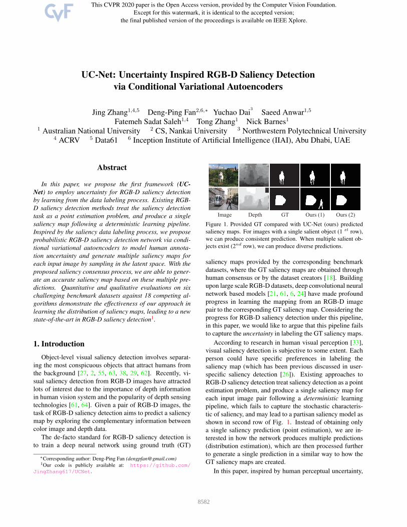
Figure 2. Network training pipeline. Four main modules are included, namely a LatentNet (PriorNet (µprior, σprior) and PosteriorNet
(µpost, σpost)), a SaliencyNet, a DepthCorrectionNet and a PredictionNet. The LatentNet maps the RGB-D image pair X (or together
with GT Y for the PosteriorNet) to low dimensional Gaussian latent variable z. The DepthCorrectionNet refines the raw depth with a
semantic guided loss. The SaliencyNet takes the RGB image and the refined depth as input to generate a saliency feature map. The
PredictionNet takes both stochastic features and deterministic features to produce a final saliency map. We perform saliency consensus in
the testing stage, as shown in Fig. 3 to generate the final saliency map according to the mechanism of GT saliency map generation.
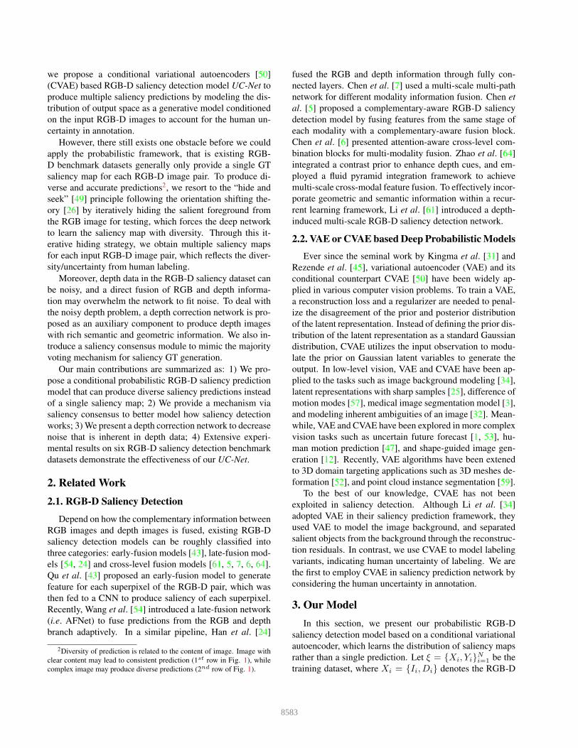
Saliency
Map
DepthCorrectionNet
SaliencyNet& PredictionNet
PriorNet
Saliency
ConcensusRGB-D
data
Sampling
C
…
… …
Figure 3. Overview of the proposed framework during testing. We
sample the PriorNet multiple times to generate diverse and accu-
rate predictions. The saliency consensus module is then used to
obtain the majority voting of the final predictions.
input (consisting of the RGB image Ii and the depth image
Di), Yi denotes the ground truth saliency map. The whole
pipeline of our model during training and testing are illus-
trated in Fig. 2 and Fig. 3, respectively.
Our network is composed of five main modules: 1) La-
tentNet (PriorNet and PosteriorNet) that maps the RGB-D
input Xi (for PriorNet) or Xi and Yi (for PosteriorNet) to
the low dimensional latent variables zi ∈ RK (K is dimen-
sion of the latent space); 2) DepthCorrectionNet that takes
Ii and Di as input to generate a refined depth image D′i;
3) SaliencyNet that maps the RGB image Ii and the refined
depth image D′i to saliency feature maps Sd
i ; 4) Prediction-
Net that employs stochastic features Ssi from LatentNet and
deterministic features Sdi from SaliencyNet to produce our
saliency map prediction Pi; 5) A saliency consensus module
in the testing stage that mimics the mechanism of saliency
GT generation to evaluate the performance with the pro-
vided single GT saliency map Yi. We will introduce each
module as follows.
3.1. Probabilistic RGBD Saliency Model via CVAE
The Conditional Variational Autoencoder (CVAE) mod-
ulates the prior as a Gaussian distribution with parameters
conditioned on the input data X . There are three types of
variables in the conditional generative model: condition-
ing variable X (RGB-D image pair in our setting), latent
variable z, and output variable Y . For the latent variable zdrawn from the Gaussian distribution Pθ(z|X), the output
variable Y is generated from Pω(Y |X, z), then the poste-
rior of z is formulated as Qφ(z|X,Y ). The loss of CVAE is
defined as:
LCVAE = Ez∼Qφ(z|X,Y )[− logPω(Y |X, z)]
+DKL(Qφ(z|X,Y )||Pθ(z|X)),(1)
where Pω(Y |X, z) is the likelihood of P (Y ) given la-
tent variable z and conditioning variable X , the Kullback-
Leibler Divergence DKL(Qφ(z|X,Y )||Pθ(z|X)) works as
a regularization loss to reduce the gap between the prior
Pθ(z|X) and the auxiliary posterior Qφ(z|X,Y ). In this
way, CVAE aims to model the log likelihood P (Y ) un-
der encoding error DKL(Qφ(z|X,Y )||Pθ(z|X)). Follow-
ing the standard practice in conventional CVAE [50], we
design a CVAE-based RGB-D saliency detection network,
and describe each component of our model in the following.
LatentNet: We define Pθ(z|X) as PriorNet that maps the
input RGB-D image pair X to a low-dimensional latent fea-
ture space, where θ is the parameter set of PriorNet. With
the same network structure and provided GT saliency map
Y , we define Qφ(z|X,Y ) as PosteriorNet, with φ being
the posterior net parameter set. In the LatentNet (Prior-
Net and PosteriorNet), we use five convolutional layers to
map the input RGB-D image X (or concatenation of Xand Y for the PosteriorNet) to the latent Gaussian variable
z ∼ N (µ, diag(σ2)), where µ, σ ∈ RK , representing the
8584
c1_4K c1_3K c1_2K
c1_K GAP
c1_K GAP
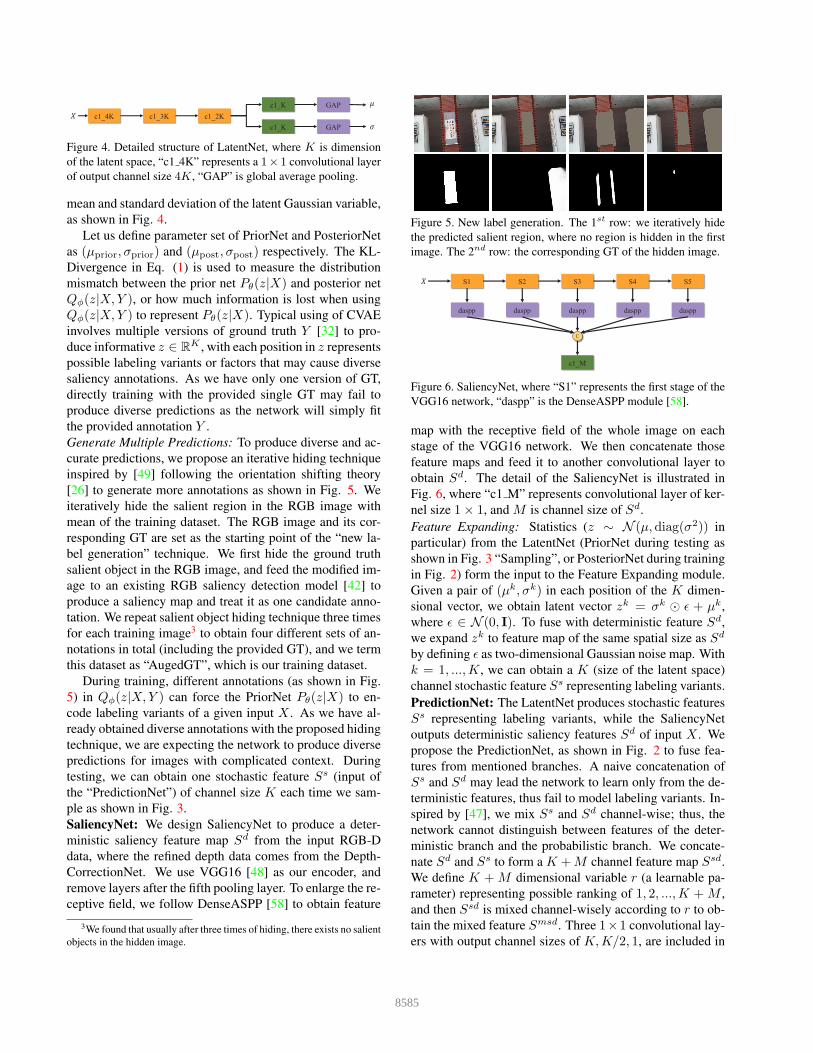
Figure 4. Detailed structure of LatentNet, where K is dimension
of the latent space, “c1 4K” represents a 1× 1 convolutional layer
of output channel size 4K, “GAP” is global average pooling.
mean and standard deviation of the latent Gaussian variable,
as shown in Fig. 4.
Let us define parameter set of PriorNet and PosteriorNet
as (µprior, σprior) and (µpost, σpost) respectively. The KL-
Divergence in Eq. (1) is used to measure the distribution
mismatch between the prior net Pθ(z|X) and posterior net
Qφ(z|X,Y ), or how much information is lost when using
Qφ(z|X,Y ) to represent Pθ(z|X). Typical using of CVAE
involves multiple versions of ground truth Y [32] to pro-
duce informative z ∈ RK , with each position in z represents
possible labeling variants or factors that may cause diverse
saliency annotations. As we have only one version of GT,
directly training with the provided single GT may fail to
produce diverse predictions as the network will simply fit
the provided annotation Y .
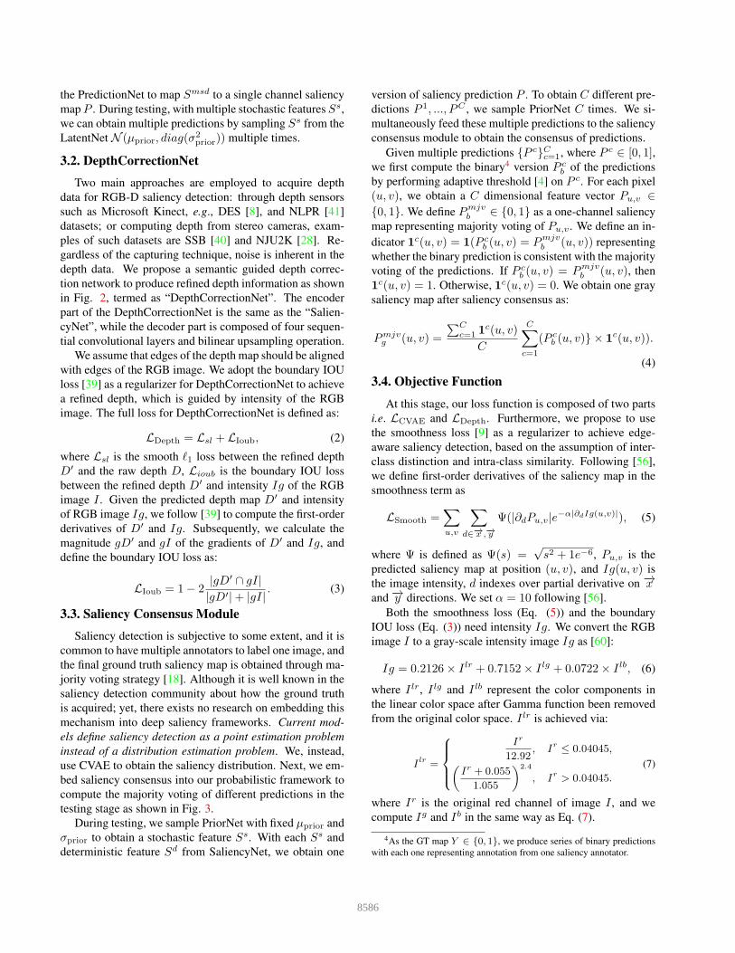
Generate Multiple Predictions: To produce diverse and ac-
curate predictions, we propose an iterative hiding technique
inspired by [49] following the orientation shifting theory
[26] to generate more annotations as shown in Fig. 5. We
iteratively hide the salient region in the RGB image with
mean of the training dataset. The RGB image and its cor-
responding GT are set as the starting point of the “new la-
bel generation” technique. We first hide the ground truth
salient object in the RGB image, and feed the modified im-
age to an existing RGB saliency detection model [42] to
produce a saliency map and treat it as one candidate anno-
tation. We repeat salient object hiding technique three times
for each training image3 to obtain four different sets of an-
notations in total (including the provided GT), and we term
this dataset as “AugedGT”, which is our training dataset.
During training, different annotations (as shown in Fig.
5) in Qφ(z|X,Y ) can force the PriorNet Pθ(z|X) to en-
code labeling variants of a given input X . As we have al-
ready obtained diverse annotations with the proposed hiding
technique, we are expecting the network to produce diverse
predictions for images with complicated context. During
testing, we can obtain one stochastic feature Ss (input of
the “PredictionNet”) of channel size K each time we sam-
ple as shown in Fig. 3.
SaliencyNet: We design SaliencyNet to produce a deter-
ministic saliency feature map Sd from the input RGB-D
data, where the refined depth data comes from the Depth-
CorrectionNet. We use VGG16 [48] as our encoder, and
remove layers after the fifth pooling layer. To enlarge the re-
ceptive field, we follow DenseASPP [58] to obtain feature
3We found that usually after three times of hiding, there exists no salient
objects in the hidden image.
Figure 5. New label generation. The 1st row: we iteratively hide
the predicted salient region, where no region is hidden in the first
image. The 2nd row: the corresponding GT of the hidden image.
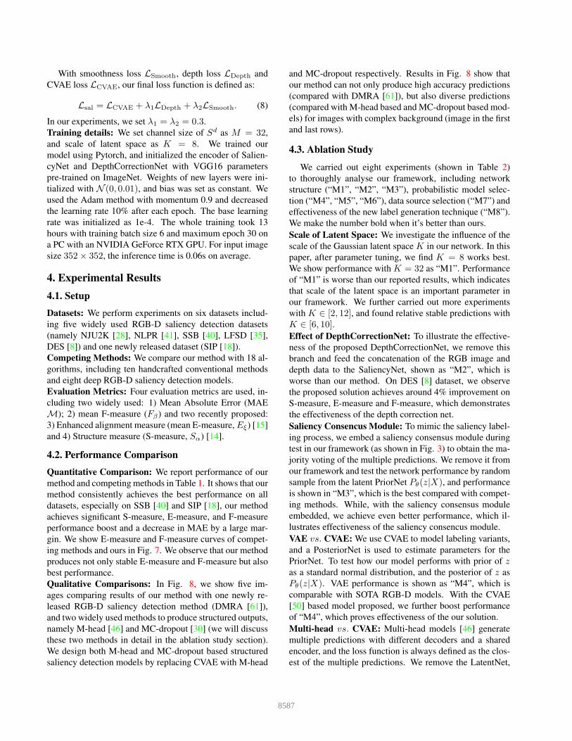
S1 S2 S3 S4 S5
daspp daspp daspp daspp daspp
C
c1_M
Figure 6. SaliencyNet, where “S1” represents the first stage of the
VGG16 network, “daspp” is the DenseASPP module [58].
map with the receptive field of the whole image on each
stage of the VGG16 network. We then concatenate those
feature maps and feed it to another convolutional layer to
obtain Sd. The detail of the SaliencyNet is illustrated in
Fig. 6, where “c1 M” represents convolutional layer of ker-
nel size 1× 1, and M is channel size of Sd.
Feature Expanding: Statistics (z ∼ N (µ, diag(σ2)) in
particular) from the LatentNet (PriorNet during testing as
shown in Fig. 3 “Sampling”, or PosteriorNet during training
in Fig. 2) form the input to the Feature Expanding module.
Given a pair of (µk, σk) in each position of the K dimen-
sional vector, we obtain latent vector zk = σk ⊙ ǫ + µk,
where ǫ ∈ N (0, I). To fuse with deterministic feature Sd,
we expand zk to feature map of the same spatial size as Sd
by defining ǫ as two-dimensional Gaussian noise map. With
k = 1, ...,K, we can obtain a K (size of the latent space)
channel stochastic feature Ss representing labeling variants.
PredictionNet: The LatentNet produces stochastic features
Ss representing labeling variants, while the SaliencyNet
outputs deterministic saliency features Sd of input X . We
propose the PredictionNet, as shown in Fig. 2 to fuse fea-
tures from mentioned branches. A naive concatenation of
Ss and Sd may lead the network to learn only from the de-
terministic features, thus fail to model labeling variants. In-
spired by [47], we mix Ss and Sd channel-wise; thus, the
network cannot distinguish between features of the deter-
ministic branch and the probabilistic branch. We concate-
nate Sd and Ss to form a K +M channel feature map Ssd.
We define K + M dimensional variable r (a learnable pa-
rameter) representing possible ranking of 1, 2, ...,K + M ,
and then Ssd is mixed channel-wisely according to r to ob-
tain the mixed feature Smsd. Three 1×1 convolutional lay-
ers with output channel sizes of K,K/2, 1, are included in
8585
the PredictionNet to map Smsd to a single channel saliency
map P . During testing, with multiple stochastic features Ss,
we can obtain multiple predictions by sampling Ss from the
LatentNet N (µprior, diag(σ2prior)) multiple times.
3.2. DepthCorrectionNet
Two main approaches are employed to acquire depth
data for RGB-D saliency detection: through depth sensors
such as Microsoft Kinect, e.g., DES [8], and NLPR [41]
datasets; or computing depth from stereo cameras, exam-
ples of such datasets are SSB [40] and NJU2K [28]. Re-
gardless of the capturing technique, noise is inherent in the
depth data. We propose a semantic guided depth correc-
tion network to produce refined depth information as shown
in Fig. 2, termed as “DepthCorrectionNet”. The encoder
part of the DepthCorrectionNet is the same as the “Salien-
cyNet”, while the decoder part is composed of four sequen-
tial convolutional layers and bilinear upsampling operation.
We assume that edges of the depth map should be aligned
with edges of the RGB image. We adopt the boundary IOU
loss [39] as a regularizer for DepthCorrectionNet to achieve
a refined depth, which is guided by intensity of the RGB
image. The full loss for DepthCorrectionNet is defined as:
LDepth = Lsl + LIoub, (2)
where Lsl is the smooth ℓ1 loss between the refined depth
D′ and the raw depth D, Lioub is the boundary IOU loss
between the refined depth D′ and intensity Ig of the RGB
image I . Given the predicted depth map D′ and intensity
of RGB image Ig, we follow [39] to compute the first-order
derivatives of D′ and Ig. Subsequently, we calculate the
magnitude gD′ and gI of the gradients of D′ and Ig, and
define the boundary IOU loss as:
LIoub = 1− 2|gD′ ∩ gI||gD′|+ |gI| . (3)
3.3. Saliency Consensus Module
Saliency detection is subjective to some extent, and it is
common to have multiple annotators to label one image, and
the final ground truth saliency map is obtained through ma-
jority voting strategy [18]. Although it is well known in the
saliency detection community about how the ground truth
is acquired; yet, there exists no research on embedding this
mechanism into deep saliency frameworks. Current mod-
els define saliency detection as a point estimation problem
instead of a distribution estimation problem. We, instead,
use CVAE to obtain the saliency distribution. Next, we em-
bed saliency consensus into our probabilistic framework to
compute the majority voting of different predictions in the
testing stage as shown in Fig. 3.
During testing, we sample PriorNet with fixed µprior and
σprior to obtain a stochastic feature Ss. With each Ss and
deterministic feature Sd from SaliencyNet, we obtain one
version of saliency prediction P . To obtain C different pre-
dictions P 1, ..., PC , we sample PriorNet C times. We si-
multaneously feed these multiple predictions to the saliency
consensus module to obtain the consensus of predictions.
Given multiple predictions {P c}Cc=1, where P c ∈ [0, 1],we first compute the binary4 version P c
b of the predictions
by performing adaptive threshold [4] on P c. For each pixel
(u, v), we obtain a C dimensional feature vector Pu,v ∈{0, 1}. We define Pmjv
b ∈ {0, 1} as a one-channel saliency
map representing majority voting of Pu,v . We define an in-
dicator 1c(u, v) = 1(P cb (u, v) = Pmjv
b (u, v)) representing
whether the binary prediction is consistent with the majority
voting of the predictions. If P cb (u, v) = Pmjv
b (u, v), then
1c(u, v) = 1. Otherwise, 1c(u, v) = 0. We obtain one gray
saliency map after saliency consensus as:
Pmjvg (u, v) =
∑Cc=1 1
c(u, v)
C
C∑
c=1
(P cb (u, v)} × 1
c(u, v)).
(4)
3.4. Objective Function
At this stage, our loss function is composed of two parts
i.e. LCVAE and LDepth. Furthermore, we propose to use
the smoothness loss [9] as a regularizer to achieve edge-
aware saliency detection, based on the assumption of inter-
class distinction and intra-class similarity. Following [56],
we define first-order derivatives of the saliency map in the
smoothness term as
LSmooth =∑
u,v
∑
d∈−→x ,−→y
Ψ(|∂dPu,v|e−α|∂dIg(u,v)|), (5)
where Ψ is defined as Ψ(s) =√s2 + 1e−6, Pu,v is the
predicted saliency map at position (u, v), and Ig(u, v) is
the image intensity, d indexes over partial derivative on −→xand −→y directions. We set α = 10 following [56].
Both the smoothness loss (Eq. (5)) and the boundary
IOU loss (Eq. (3)) need intensity Ig. We convert the RGB
image I to a gray-scale intensity image Ig as [60]:
Ig = 0.2126× I lr + 0.7152× I lg + 0.0722× I lb, (6)
where I lr, I lg and I lb represent the color components in
the linear color space after Gamma function been removed
from the original color space. I lr is achieved via:
Ilr =
Ir
12.92, I
r≤ 0.04045,
(
Ir + 0.055
1.055
)2.4
, Ir> 0.04045.
(7)
where Ir is the original red channel of image I , and we
compute Ig and Ib in the same way as Eq. (7).
4As the GT map Y ∈ {0, 1}, we produce series of binary predictions
with each one representing annotation from one saliency annotator.
8586
With smoothness loss LSmooth, depth loss LDepth and
CVAE loss LCVAE, our final loss function is defined as:
Lsal = LCVAE + λ1LDepth + λ2LSmooth. (8)
In our experiments, we set λ1 = λ2 = 0.3.
Training details: We set channel size of Sd as M = 32,
and scale of latent space as K = 8. We trained our
model using Pytorch, and initialized the encoder of Salien-
cyNet and DepthCorrectionNet with VGG16 parameters
pre-trained on ImageNet. Weights of new layers were ini-
tialized with N (0, 0.01), and bias was set as constant. We
used the Adam method with momentum 0.9 and decreased
the learning rate 10% after each epoch. The base learning
rate was initialized as 1e-4. The whole training took 13
hours with training batch size 6 and maximum epoch 30 on
a PC with an NVIDIA GeForce RTX GPU. For input image
size 352× 352, the inference time is 0.06s on average.
4. Experimental Results
4.1. Setup
Datasets: We perform experiments on six datasets includ-
ing five widely used RGB-D saliency detection datasets
(namely NJU2K [28], NLPR [41], SSB [40], LFSD [35],
DES [8]) and one newly released dataset (SIP [18]).
Competing Methods: We compare our method with 18 al-
gorithms, including ten handcrafted conventional methods
and eight deep RGB-D saliency detection models.
Evaluation Metrics: Four evaluation metrics are used, in-
cluding two widely used: 1) Mean Absolute Error (MAE
M); 2) mean F-measure (Fβ) and two recently proposed:
3) Enhanced alignment measure (mean E-measure, Eξ) [15]
and 4) Structure measure (S-measure, Sα) [14].
4.2. Performance Comparison
Quantitative Comparison: We report performance of our
method and competing methods in Table 1. It shows that our
method consistently achieves the best performance on all
datasets, especially on SSB [40] and SIP [18], our method
achieves significant S-measure, E-measure, and F-measure
performance boost and a decrease in MAE by a large mar-
gin. We show E-measure and F-measure curves of compet-
ing methods and ours in Fig. 7. We observe that our method
produces not only stable E-measure and F-measure but also
best performance.
Qualitative Comparisons: In Fig. 8, we show five im-
ages comparing results of our method with one newly re-
leased RGB-D saliency detection method (DMRA [61]),
and two widely used methods to produce structured outputs,
namely M-head [46] and MC-dropout [30] (we will discuss
these two methods in detail in the ablation study section).
We design both M-head and MC-dropout based structured
saliency detection models by replacing CVAE with M-head
and MC-dropout respectively. Results in Fig. 8 show that
our method can not only produce high accuracy predictions
(compared with DMRA [61]), but also diverse predictions
(compared with M-head based and MC-dropout based mod-
els) for images with complex background (image in the first
and last rows).
4.3. Ablation Study
We carried out eight experiments (shown in Table 2)
to thoroughly analyse our framework, including network
structure (“M1”, “M2”, “M3”), probabilistic model selec-
tion (“M4”, “M5”, “M6”), data source selection (“M7”) and
effectiveness of the new label generation technique (“M8”).
We make the number bold when it’s better than ours.
Scale of Latent Space: We investigate the influence of the
scale of the Gaussian latent space K in our network. In this
paper, after parameter tuning, we find K = 8 works best.
We show performance with K = 32 as “M1”. Performance
of “M1” is worse than our reported results, which indicates
that scale of the latent space is an important parameter in
our framework. We further carried out more experiments
with K ∈ [2, 12], and found relative stable predictions with
K ∈ [6, 10].
Effect of DepthCorrectionNet: To illustrate the effective-
ness of the proposed DepthCorrectionNet, we remove this
branch and feed the concatenation of the RGB image and
depth data to the SaliencyNet, shown as “M2”, which is
worse than our method. On DES [8] dataset, we observe
the proposed solution achieves around 4% improvement on
S-measure, E-measure and F-measure, which demonstrates
the effectiveness of the depth correction net.
Saliency Consencus Module: To mimic the saliency label-
ing process, we embed a saliency consensus module during
test in our framework (as shown in Fig. 3) to obtain the ma-
jority voting of the multiple predictions. We remove it from
our framework and test the network performance by random
sample from the latent PriorNet Pθ(z|X), and performance
is shown in “M3”, which is the best compared with compet-
ing methods. While, with the saliency consensus module
embedded, we achieve even better performance, which il-
lustrates effectiveness of the saliency consencus module.
VAE vs. CVAE: We use CVAE to model labeling variants,
and a PosteriorNet is used to estimate parameters for the
PriorNet. To test how our model performs with prior of zas a standard normal distribution, and the posterior of z as
Pθ(z|X). VAE performance is shown as “M4”, which is
comparable with SOTA RGB-D models. With the CVAE
[50] based model proposed, we further boost performance
of “M4”, which proves effectiveness of the our solution.
Multi-head vs. CVAE: Multi-head models [46] generate
multiple predictions with different decoders and a shared
encoder, and the loss function is always defined as the clos-
est of the multiple predictions. We remove the LatentNet,
8587
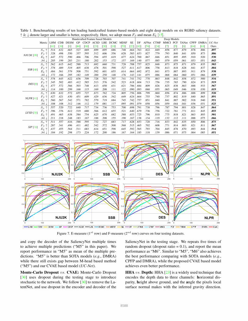
Table 1. Benchmarking results of ten leading handcrafted feature-based models and eight deep models on six RGBD saliency datasets.
↑ & ↓ denote larger and smaller is better, respectively. Here, we adopt mean Fβ and mean Eξ [15].Handcrafted Feature based Models Deep Models
Metric LHM CDB DESM GP CDCP ACSD LBE DCMC MDSF SE DF AFNet CTMF MMCI PCF TANet CPFP DMRA UC-Net
[41] [36] [8] [44] [66] [28] [20] [10] [51] [22] [43] [54] [24] [7] [5] [6] [64] [61] Ours
NJU2K [28]
Sα ↑ .514 .632 .665 .527 .669 .699 .695 .686 .748 .664 .763 .822 .849 .858 .877 .879 .878 .886 .897
Fβ ↑ .328 .498 .550 .357 .595 .512 .606 .556 .628 .583 .653 .827 .779 .793 .840 .841 .850 .873 .886
Eξ ↑ .447 .572 .590 .466 .706 .594 .655 .619 .677 .624 .700 .867 .846 .851 .895 .895 .910 .920 .930
M ↓ .205 .199 .283 .211 .180 .202 .153 .172 .157 .169 .140 .077 .085 .079 .059 .061 .053 .051 .043
SSB [40]
Sα ↑ .562 .615 .642 .588 .713 .692 .660 .731 .728 .708 .757 .825 .848 .873 .875 .871 .879 .835 .903
Fβ ↑ .378 .489 .519 .405 .638 .478 .501 .590 .527 .611 .617 .806 .758 .813 .818 .828 .841 .837 .884
Eξ ↑ .484 .561 .579 .508 .751 .592 .601 .655 .614 .664 .692 .872 .841 .873 .887 .893 .911 .879 .938
M ↓ .172 .166 .295 .182 .149 .200 .250 .148 .176 .143 .141 .075 .086 .068 .064 .060 .051 .066 .039
DES [8]
Sα ↑ .578 .645 .622 .636 .709 .728 .703 .707 .741 .741 .752 .770 .863 .848 .842 .858 .872 .900 .934
Fβ ↑ .345 .502 .483 .412 .585 .513 .576 .542 .523 .618 .604 .713 .756 .735 .765 .790 .824 .873 .919
Eξ ↑ .477 .572 .566 .503 .748 .613 .650 .631 .621 .706 .684 .809 .826 .825 .838 .863 .888 .933 .967
M ↓ .114 .100 .299 .168 .115 .169 .208 .111 .122 .090 .093 .068 .055 .065 .049 .046 .038 .030 .019
NLPR [41]
Sα ↑ .630 .632 .572 .655 .727 .673 .762 .724 .805 .756 .806 .799 .860 .856 .874 .886 .888 .899 .920
Fβ ↑ .427 .421 .430 .451 .609 .429 .636 .542 .649 .624 .664 .755 .740 .737 .802 .819 .840 .865 .891
Eξ ↑ .560 .567 .542 .571 .782 .579 .719 .684 .745 .742 .757 .851 .840 .841 .887 .902 .918 .940 .951
M ↓ .108 .108 .312 .146 .112 .179 .081 .117 .095 .091 .079 .058 .056 .059 .044 .041 .036 .031 .025
LFSD [35]
Sα ↑ .557 .520 .722 .640 .717 .734 .736 .753 .700 .698 .791 .738 .796 .787 .794 .801 .828 .847 .864
Fβ ↑ .396 .376 .612 .519 .680 .566 .612 .655 .521 .640 .679 .736 .756 .722 .761 .771 .811 .845 .855
Eξ ↑ .491 .465 .638 .584 .754 .625 .670 .682 .588 .653 .725 .796 .810 .775 .818 .821 .863 .893 .901
M ↓ .211 .218 .248 .183 .167 .188 .208 .155 .190 .167 .138 .134 .119 .132 .112 .111 .088 .075 .066
SIP [18]
Sα ↑ .511 .557 .616 .588 .595 .732 .727 .683 .717 .628 .653 .720 .716 .833 .842 .835 .850 .806 .875
Fβ ↑ .287 .341 .496 .411 .482 .542 .572 .500 .568 .515 .465 .702 .608 .771 .814 .803 .821 .811 .867
Eξ ↑ .437 .455 .564 .511 .683 .614 .651 .598 .645 .592 .565 .793 .704 .845 .878 .870 .893 .844 .914
M ↓ .184 .192 .298 .173 .224 .172 .200 .186 .167 .164 .185 .118 .139 .086 .071 .075 .064 .085 .051
0 100 256
0.2
0.4
0.6
0.8
1
NJU2K
0 100 256
0.2
0.4
0.6
0.8
1
SSB
0 100 256
0
0.2
0.4
0.6
0.8
1
DES
0 100 256
0
0.2
0.4
0.6
0.8
NJU2K
0 100 256
0
0.2
0.4
0.6
0.8
SSB
0 100 256
0
0.2
0.4
0.6
0.8
1
DES
0 100 256
0
0.2
0.4
0.6
0.8
1
NLPR
0 100 256
0.2
0.4
0.6
0.8
1
NLPR
Figure 7. E-measure (1st row) and F-measure (2nd row) curves on four testing datasets.
and copy the decoder of the SaliencyNet multiple times
to achieve multiple predictions (“M5” in this paper). We
report performance in “M5” as mean of the multiple pre-
dictions. “M5” is better than SOTA models (e.g., DMRA)
while there still exists gap between M-head based method
(“M5”) and our CVAE based model (UC-Net).
Monte-Carlo Dropout vs. CVAE: Monte-Carlo Dropout
[30] uses dropout during the testing stage to introduce
stochastic to the network. We follow [30] to remove the La-
tentNet, and use dropout in the encoder and decoder of the
SaliencyNet in the testing stage. We repeats five times of
random dropout (dropout ratio = 0.1), and report the mean
performance as “M6”. Similar to “M5”, “M6” also achieves
the best performance comparing with SOTA models (e.g.,
CPFP and DMRA), while the proposed CVAE based model
achieves even better performance.
HHA vs. Depth: HHA [23] is a widely used technique that
encodes the depth data to three channels: horizontal dis-
parity, height above ground, and the angle the pixels local
surface normal makes with the inferred gravity direction.
8588

)2( sruO)1( sruOTGhtpeDegamI UC-NetDMRA MH1 MH2 DP1 DP2
Figure 8. Comparisons of saliency maps. “MH1” and “MH2” are two predictions from M-head. “DP1” and “DP2” are predictions of
two random MC-dropout during test. “Ours(1)” and “Ours(2)” are two predictions sampled from our CVAE based model. Different from
M-head and MC-dropout, which produce consistent predictions for ambiguous images (5th row), UC-Net can produce diverse predictions.
Table 2. Ablation study on RGB-D saliency datasets.Metric UC-Net M1 M2 M3 M4 M5 M6 M7 M8 M9
NJU
2K
[28
]
Sα ↑ .897 .866 .893 .905 .871 .885 .881 .893 .838 .866
Fβ ↑ .886 .858 .887 .884 .851 .878 .878 .884 .787 .812
Eξ ↑ .930 .905 .930 .927 .910 .923 .927 .932 .840 .866
M ↓ .043 .060 .046 .045 .059 .047 .046 .044 .084 .075
SSB
[40
] Sα ↑ .903 .854 .893 .900 .867 .891 .893 .898 .855 .872
Fβ ↑ .884 .831 .876 .868 .834 .864 .876 .882 .793 .805
Eξ ↑ .938 .894 .911 .922 .907 .921 .931 .934 .854 .870
M ↓ .039 .060 .043 .047 .057 .047 .043 .040 .073 .068
DE
S[8
] Sα ↑ .934 .876 .896 .928 .897 .911 .896 .918 .811 .911
Fβ ↑ .919 .844 .868 .902 .867 .897 .868 .904 .724 .843
Eξ ↑ .967 .906 .928 .947 .930 .945 .928 .953 .794 .910
M ↓ .019 .035 .026 .024 .033 .024 .026 .023 .065 .036
NL
PR
[41
] Sα ↑ .920 .878 .919 .918 .890 .899 .910 .915 .850 .883
Fβ ↑ .891 .846 .897 .878 .845 .875 .867 .889 .759 .795
Eξ ↑ .951 .911 .953 .941 .924 .937 .933 .951 .841 .883
M ↓ .025 .039 .024 .029 .037 .029 .028 .025 .057 .045
LF
SD
[35
] Sα ↑ .864 .799 .847 .862 .820 .838 .847 .853 .729 .823
Fβ ↑ .855 .791 .838 .841 .802 .833 .838 .848 .661 .779
Eξ ↑ .901 .829 .879 .885 .865 .875 .879 .891 .720 .818
M ↓ .066 .101 .079 .075 .093 .079 .079 .073 .145 .108
SIP
[18
] Sα ↑ .875 .846 .867 .870 .851 .859 .867 .865 .810 .845
Fβ ↑ .867 .837 .860 .848 .821 .853 .860 .855 .751 .795
Eξ ↑ .914 .884 .908 .901 .893 .905 .908 .908 .816 .852
M ↓ .051 .068 .056 .059 .067 .057 .056 .056 .094 .079
HHA is widely used in RGB-D related dense prediction
models [11, 24] to obtain better feature representation. To
test if HHA also works in our scenario, we replace depth
with HHA, and performance is shown in “M7”. We observe
similar performance achieved with HHA instead of the raw
depth data.
New Label Generation: To produce diverse predictions,
we follow [49] and generate diverse annotations for the
training dataset. To illustrate the effectiveness of this strat-
egy, we train with only the SaliencyNet to produce single
channel saliency map with RGB-D image as input for sim-
plicity. “M8” and “M9” represent using the provided train-
ing dataset and augmented training data respectively. We
observe performance improvement of “M9” compared with
“M8”, which indicates effectiveness of the new label gener-
ation technique.
5. Conclusion
Inspired by human uncertainty in ground truth (GT) an-
notation, we proposed the first uncertainty network named
UC-Net for RGB-D saliency detection based on a con-
ditional variational autoencoder. Different from existing
methods, which generally treat saliency detection as a point
estimation problem, we propose to learn the distribution
of saliency maps. Under our formulation, our model is
able to generate multiple labels which have been discarded
in the GT annotation generation process through saliency
consensus. Quantitative and qualitative evaluations on six
standard and challenging benchmark datasets demonstrated
the superiority of our approach in learning the distribution
of saliency maps. In the future, we would like to extend
our approach to other saliency detection problems (e.g.,
VSOD [19], RGB SOD [13, 65], Co-SOD [17]). Further-
more, we plan to capture new datasets with multiple human
annotations to further model the statistics of human uncer-
tainty in interactive image segmentation [37], camouflaged
object detection [16], etc.
Acknowledgments. This research was supported in part
by Natural Science Foundation of China grants (61871325,
61420106007, 61671387), the Australia Research Council Centre
of Excellence for Robotics Vision (CE140100016), and the Na-
tional Key Research and Development Program of China under
Grant 2018AAA0102803. We thank all reviewers and Area Chairs
for their constructive comments.
8589
References
[1] Abubakar Abid and James Y. Zou. Contrastive Vari-
ational Autoencoder Enhances Salient Features. CoRR,
abs/1902.04601, 2019.
[2] Radhakrishna Achanta, Sheila Hemami, Francisco Estrada,
and Sabine Susstrunk. Frequency-tuned salient region detec-
tion. In IEEE CVPR, pages 1597–1604, 2009.
[3] Christian F. Baumgartner, Kerem Can Tezcan, Krishna Chai-
tanya, Andreas M. Hotker, Urs J. Muehlematter, Khoschy
Schawkat, Anton S. Becker, Olivio Donati, and Ender
Konukoglu. PHiSeg: Capturing Uncertainty in Medical Im-
age Segmentation. In MICCAI, pages 119–127, 2019.
[4] Ali Borji, Ming-Ming Cheng, Huaizu Jiang, and Jia Li.
Salient Object Detection: A Benchmark. IEEE TIP,
24(12):5706–5722, 2015.
[5] Hao Chen and Youfu Li. Progressively complementarity-
aware fusion network for RGB-D Salient Object Detection.
In IEEE CVPR, pages 3051–3060, 2018.
[6] Hao Chen and Youfu Li. Three-stream Attention-aware Net-
work for RGB-D Salient Object Detection. IEEE TIP, pages
2825–2835, 2019.
[7] Hao Chen, Youfu Li, and Dan Su. Multi-modal fusion net-
work with multi-scale multi-path and cross-modal interac-
tions for RGB-D salient object detection. PR, 86:376–385,
2019.
[8] Yupeng Cheng, Huazhu Fu, Xingxing Wei, Jiangjian Xiao,
and Xiaochun Cao. Depth enhanced saliency detection
method. In ACM ICIMCS, pages 23–27, 2014.
[9] Gabriel J. Brostow Clment Godard, Oisin Mac Aodha. Unsu-
pervised Monocular Depth Estimation with Left-Right Con-
sistency. In IEEE CVPR, pages 6602–6611, 2017.
[10] Runmin Cong, Jianjun Lei, Changqing Zhang, Qingming
Huang, Xiaochun Cao, and Chunping Hou. Saliency detec-
tion for stereoscopic images based on depth confidence anal-
ysis and multiple cues fusion. IEEE SPL, 23(6):819–823,
2016.
[11] Dapeng Du, Limin Wang, Huiling Wang, Kai Zhao, and
Gangshan Wu. Translate-to-Recognize Networks for RGB-
D Scene Recognition. In IEEE CVPR, pages 11836–11845,
2019.
[12] Patrick Esser, Ekaterina Sutter, and Bjrn Ommer. A Varia-
tional U-Net for Conditional Appearance and Shape Gener-
ation. In IEEE CVPR, pages 8857–8865, 2018.
[13] Deng-Ping Fan, Ming-Ming Cheng, Jiang-Jiang Liu, Shang-
Hua Gao, Qibin Hou, and Ali Borji. Salient objects in clut-
ter: Bringing salient object detection to the foreground. In
ECCV, pages 186–202, 2018.
[14] Deng-Ping Fan, Ming-Ming Cheng, Yun Liu, Tao Li, and Ali
Borji. Structure-measure: A new way to evaluate foreground
maps. In IEEE ICCV, pages 4548–4557, 2017.
[15] Deng-Ping Fan, Cheng Gong, Yang Cao, Bo Ren, Ming-
Ming Cheng, and Ali Borji. Enhanced-alignment Measure
for Binary Foreground Map Evaluation. In IJCAI, pages
698–704, 2018.
[16] Deng-Ping Fan, Ge-Peng Ji, Guolei Sun, Ming-Ming Cheng,
Jianbing Shen, and Ling Shao. Camouflaged Object Detec-
tion. In IEEE CVPR, 2020.
[17] Deng-Ping Fan, Zheng Lin, Ge-Peng Ji, Dingwen Zhang,
Huazhu Fu, and Ming-Ming Cheng. Taking a Deeper Look
at the Co-salient Object Detection. In IEEE CVPR, 2020.
[18] Deng-Ping Fan, Zheng Lin, Zhao Zhang, Menglong Zhu, and
Ming-Ming Cheng. Rethinking RGB-D salient object detec-
tion: Models, datasets, and large-scale benchmarks. IEEE
TNNLS, 2020.
[19] Deng-Ping Fan, Wenguan Wang, Ming-Ming Cheng, and
Jianbing Shen. Shifting more attention to video salient object
detection. In IEEE CVPR, pages 8554–8564, 2019.
[20] David Feng, Nick Barnes, Shaodi You, and Chris McCarthy.
Local background enclosure for RGB-D salient object detec-
tion. In IEEE CVPR, pages 2343–2350, 2016.
[21] Keren Fu Fu, Deng-Ping Fan, Ge-Peng Ji, and Qijun Zhao.
JL-DCF: Joint Learning and Densely-Cooperative Fusion
Framework for RGB-D Salient Object Detection. In IEEE
CVPR, 2020.
[22] Jingfan Guo, Tongwei Ren, and Jia Bei. Salient object detec-
tion for rgb-d image via saliency evolution. In ICME, pages
1–6, 2016.
[23] Saurabh Gupta, Ross Girshick, Pablo Arbelaez, and Jitendra
Malik. Learning rich features from RGB-D images for object
detection and segmentation. In ECCV, pages 345–360, 2014.
[24] Junwei Han, Hao Chen, Nian Liu, Chenggang Yan, and Xue-
long Li. CNNs-based RGB-D saliency detection via cross-
view transfer and multiview fusion. IEEE TCYB, pages
3171–3183, 2018.
[25] Faruk Ahmed Adrien Ali Taga Francesco Visin David
Vzquez Aaron C. Courville Ishaan Gulrajani, Kundan Ku-
mar. PixelVAE: A Latent Variable Model for Natural Images.
In ICLR, 2016.
[26] Laurent Itti and Christof Koch. A saliency-based search
mechanism for overt and covert shifts of visual attention. VR,
40(10):1489 – 1506, 2000.
[27] Laurent Itti, Christof Koch, and Ernst Niebur. A model
of saliency-based visual attention for rapid scene analysis.
IEEE TPAMI, 20(11):1254–1259, 1998.
[28] Ran Ju, Ling Ge, Wenjing Geng, Tongwei Ren, and Gang-
shan Wu. Depth saliency based on anisotropic center-
surround difference. In ICIP, pages 1115–1119, 2014.
[29] Shuhui Wang Jun Wei and Qingming Huang. F3Net: Fusion,
Feedback and Focus for Salient Object Detection. In AAAI,
2020.
[30] Alex Kendall, Vijay Badrinarayanan, , and Roberto Cipolla.
Bayesian SegNet: Model Uncertainty in Deep Convolutional
Encoder-Decoder Architectures for Scene Understanding. In
BMVC, 2017.
[31] Diederik P Kingma and Max Welling. Auto-Encoding Vari-
ational Bayes. In ICLR, 2013.
[32] Simon Kohl, Bernardino Romera-Paredes, Clemens Meyer,
Jeffrey De Fauw, Joseph R. Ledsam, Klaus Maier-Hein,
S. M. Ali Eslami, Danilo Jimenez Rezende, and Olaf Ron-
neberger. A Probabilistic U-Net for Segmentation of Am-
biguous Images. In NeurIPS, pages 6965–6975, 2018.
[33] Olivier Le Meur and Thierry Baccino. Methods for compar-
ing scanpaths and saliency maps: strengths and weaknesses.
Behavior Research Methods, 45(1):251–266, 2013.
8590
[34] Bo Li, Zhengxing Sun, and Yuqi Guo. SuperVAE: Superpix-
elwise Variational Autoencoder for Salient Object Detection.
In AAAI, pages 8569–8576, 2019.
[35] Nianyi Li, Jinwei Ye, Yu Ji, Haibin Ling, and Jingyi Yu.
Saliency detection on light field. In IEEE CVPR, pages
2806–2813, 2014.
[36] Fangfang Liang, Lijuan Duan, Wei Ma, Yuanhua Qiao, Zhi
Cai, and Laiyun Qing. Stereoscopic saliency model using
contrast and depth-guided-background prior. Neurocomput-
ing, 275:2227–2238, 2018.
[37] Zheng Lin, Zhao Zhang, Lin-Zhuo Chen, Ming-Ming
Cheng, and Shao-Ping Lu. Interactive Image Segmentation
with First Click Attention. In IEEE CVPR, 2020.
[38] Yi Liu, Qiang Zhang, Dingwen Zhang, and Jungong Han.
Employing Deep Part-Object Relationships for Salient Ob-
ject Detection. In IEEE ICCV, 2019.
[39] Zhiming Luo, Akshaya Mishra, Andrew Achkar, Justin
Eichel, Shaozi Li, and Pierre-Marc Jodoin. Non-Local Deep
Features for Salient Object Detection. In IEEE CVPR, 2017.
[40] Yuzhen Niu, Yujie Geng, Xueqing Li, and Feng Liu. Lever-
aging stereopsis for saliency analysis. In IEEE CVPR, pages
454–461, 2012.
[41] Houwen Peng, Bing Li, Weihua Xiong, Weiming Hu, and
Rongrong Ji. Rgbd salient object detection: a benchmark
and algorithms. In ECCV, pages 92–109, 2014.
[42] Xuebin Qin, Zichen Zhang, Chenyang Huang, Chao
Gao, Masood Dehghan, and Martin Jagersand. BASNet:
Boundary-Aware Salient Object Detection. In IEEE CVPR,
2019.
[43] Liangqiong Qu, Shengfeng He, Jiawei Zhang, Jiandong
Tian, Yandong Tang, and Qingxiong Yang. RGBD salient
object detection via deep fusion. IEEE TIP, 26(5):2274–
2285, 2017.
[44] Jianqiang Ren, Xiaojin Gong, Lu Yu, Wenhui Zhou, and
Michael Ying Yang. Exploiting Global Priors for RGB-D
Saliency Detection. In IEEE CVPRW, pages 25–32, 2015.
[45] Danilo Jimenez Rezende, Shakir Mohamed, and Daan Wier-
stra. Stochastic Backpropagation and Approximate Inference
in Deep Generative Models. In ICML, pages 1278–1286,
2014.
[46] Christian Rupprecht, Iro Laina, Maximilian Baust, Federico
Tombari, Gregory D. Hager, and Nassir Navab. Learning in
an Uncertain World: Representing Ambiguity Through Mul-
tiple Hypotheses. In IEEE ICCV, pages 3611–3620, 2017.
[47] Mohammad Sadegh Aliakbarian, Fatemeh Sadat Saleh,
Mathieu Salzmann, Lars Petersson, Stephen Gould, and
Amirhossein Habibian. Learning Variations in Human Mo-
tion via Mix-and-Match Perturbation. arXiv e-prints, page
arXiv:1908.00733, 2019.
[48] Karen Simonyan and Andrew Zisserman. Very Deep Con-
volutional Networks for Large-Scale Image Recognition. In
ICLR, 2014.
[49] Krishna Kumar Singh and Yong Jae Lee. Hide-and-Seek:
Forcing a Network to be Meticulous for Weakly-supervised
Object and Action Localization. In IEEE ICCV, 2017.
[50] Kihyuk Sohn, Honglak Lee, and Xinchen Yan. Learning
Structured Output Representation using Deep Conditional
Generative Models. In NeurIPS, pages 3483–3491, 2015.
[51] Hangke Song, Zhi Liu, Huan Du, Guangling Sun, Olivier
Le Meur, and Tongwei Ren. Depth-aware salient ob-
ject detection and segmentation via multiscale discrimina-
tive saliency fusion and bootstrap learning. IEEE TIP,
26(9):4204–4216, 2017.
[52] Qingyang Tan, Lin Gao, Yu-Kun Lai, and Shihong Xia. Vari-
ational Autoencoders for Deforming 3D Mesh Models. In
IEEE CVPR, 2018.
[53] Jacob Walker, Carl Doersch, Harikrishna Mulam, and Mar-
tial Hebert. An Uncertain Future: Forecasting from Static
Images Using Variational Autoencoders. In ECCVW, pages
835–851, 2016.
[54] Ningning Wang and Xiaojin Gong. Adaptive Fusion for
RGB-D Salient Object Detection. IEEE Access, 7:55277–
55284, 2019.
[55] Wenguan Wang, Jianbing Shen, Ming-Ming Cheng, and
Ling Shao. An Iterative and Cooperative Top-Down and
Bottom-Up Inference Network for Salient Object Detection.
In IEEE CVPR, 2019.
[56] Yang Wang, Yi Yang, Zhenheng Yang, Liang Zhao, Peng
Wang, and Wei Xu. Occlusion Aware Unsupervised Learn-
ing of Optical Flow. In IEEE CVPR, 2018.
[57] Rastogi Akash Villegas Ruben Sunkavalli Kalyan Shecht-
man Eli Hadap Sunil Yumer Ersin Lee Honglak Yan,
Xinchen. MT-VAE: Learning Motion Transformations to
Generate Multimodal Human Dynamics. In ECCV, pages
276–293, 2018.
[58] Maoke Yang, Kun Yu, Chi Zhang, Zhiwei Li, and Kuiyuan
Yang. DenseASPP for Semantic Segmentation in Street
Scenes. In IEEE CVPR, pages 3684–3692, 2018.
[59] Li Yi, Wang Zhao, He Wang, Minhyuk Sung, and Leonidas J.
Guibas. GSPN: Generative Shape Proposal Network for 3D
Instance Segmentation in Point Cloud. In IEEE CVPR, 2019.
[60] Shivanthan A. C. Yohanandan, Adrian G. Dyer, Dacheng
Tao, and Andy Song. Saliency Preservation in Low-
Resolution Grayscale Images. In ECCV, 2018.
[61] Jingjing Li Miao Zhang Huchuan Lu Yongri Piao, Wei Ji.
Depth-induced Multi-scale Recurrent Attention Network for
Saliency Detection. In IEEE ICCV, 2019.
[62] Jing Zhang, Xin Yu, Aixuan Li, Peipei Song, Bowen Liu, and
Yuchao Dai. Weakly-Supervised Salient Object Detection
via Scribble Annotations. In IEEE CVPR, 2020.
[63] Jing Zhang, Tong Zhang, Yuchao Dai, Mehrtash Harandi,
and Richard Hartley. Deep Unsupervised Saliency Detec-
tion: A Multiple Noisy Labeling Perspective. In IEEE
CVPR, pages 9029–9038, 2018.
[64] Jia-Xing Zhao, Yang Cao, Deng-Ping Fan, Ming-Ming
Cheng, Xuan-Yi Li, and Le Zhang. Contrast Prior and Fluid
Pyramid Integration for RGBD Salient Object Detection. In
IEEE CVPR, 2019.
[65] Jia-Xing Zhao, Jiang-Jiang Liu, Deng-Ping Fan, Yang Cao,
Jufeng Yang, and Ming-Ming Cheng. EGNet: Edge guid-
ance network for salient object detection. In IEEE ICCV,
pages 8779–8788, 2019.
[66] Chunbiao Zhu, Ge Li, Wenmin Wang, and Ronggang Wang.
An innovative salient object detection using center-dark
channel prior. In IEEE ICCVW, 2017.
8591