AERO-ASTRONAUTICS REPORT NO. 26

THREE-DIMENSIONAL, LltIING WINGS

OF MINIMUM DRAG IN HYPERSONIC FLOW < ! I

, I

la bY

ANGEL

N 6 6 34633 UCCESSION NUMBER) WHRUI

IPAGESJ (CODE)

CR m2?/ Od TUX O R AD NUMBER) ol I C A T ~ O R I )

https://ntrs.nasa.gov/search.jsp?R=19660025343 2018-06-03T06:26:05+00:00Z

I 1 . THREE-DIMENSIONAL, LIFTING WINGS

OF MINIMUM DRAG IN HYPERSONIC FLOW(*)

I AAR-26

bY

(* * *) ANGEL0 MIELE(**) and DAVJD G. HULL

SUMMARY

The problem of minimizing the drag of a three-dimensional, slender, flat-top

wing of given span in hypersonic flow is considered under the assumptions that the

pressure coefficient is modified Newtonian and the skin-friction coefficient is constant.

The indirect methods of the calculus of variations in two independent variables are

employed, and the minimum drag problem is solved for (a) given lift and (b) given

lift and volume.

If the lift is the only given quantity, the optimum wing has a constant chordwise

slope and a trailing edge thickness distribution similar to the chord distribution.

While the planform area is uniquely determined, the chord distribution is not. In

(*) This research was supported by the Langley Research Center of the National

Aeronautics and Space Administration under Grant No. NGR-44-006-045.

(**I Professor of A S ~ ~ O M U ~ ~ C S and Director of the Aero-Astronautics Group,

Department of Mechanical and Aerospace Engineering and Materials Science, Rice

University, Houston, Texas.

..* j- .%

(- Research Associate in Astronautics , Department of Mechanical and Aerospace

Engineering and Materials Science, Rice University, Houston, Texas .

2 AAR-26

other words, there exist an infinite number of chord distributions yielding the same

maximum value of the lift-to-drag ratio.

If the lift and the volume are given, two solutions are possible depending on the

value of the volume-lift parameter, a parameter directly proportional to the volume

and inversely proportional to the lift squared. If the volume-lift parameter is greater

than a certain critical value, the optimum wing is identical with that of case (a). If the

volume-lift parameter is smaller than the critical value, the optimum wing has a con-

stant chord and a constant trailing edge thickness. Also, the chordwise slope is

constant irl ?he spanwise sense but not in the chordwise sense. Finally, the maximum

lift- to- drag ratio decreases as the volume- lift parameter decreases.

3 AAR- 26

1 . INTRODUCTION

In previous papers (Refs. 1 through 3), the problem of minimizing the zero-lift

drag of a three-dimensional wing in hypersonic flow was considered under the assumptions

that the pressure distribution is Newtonian and the skin-friction coefficient is zero o r

constant. Various conditions were imposed on the volume, the planform shape, and

the thickness distribution on the periphery of the planform.

In this paper, the problem investigated in Refs. 1 through 3 is considered once

more in connection with a wing designed to produce a specified lift. For simplicity,

the analysis is limited to the class of flat-top wings whose upper surface is parallel to

the undisturbed flow direction (Ref. 4). For these wings, the minimal problem consists

of extremizing a surface integral with a variable boundary subjected to several constraints

of the isoperimetric type.

In the following sections, the necessary conditions for the extremum are derived

in general according t o the mathematical treatment presented in Chapter 3 of Ref. 5.

Then, several particular cases are studied and solved in detail. The hypotheses employed

are as follows : (a) a plane of symmetry exists between the left- hand and right-hand

par ts of the wing; (b) the upper surface is flat; (c) the free-stream velocity is parallel

t o the line of intersection of the plane of symmetry and the flat top; (d) the wing is

slender in both the chordwise and spanwise senses, that is, the squares of both the

chordwise and spanwise slopes a re small with respect to one; (e) the pressure coef-

ficient is proportional to the cosine squared of the angle formed by the free-stream

velocity and the normal to each surface element; (f) the skin-friction coefficient is con-

stant and equal to some suitahly chosen average value; (g) the base drag is neglected;

4 AAR-26

and (h) the contribution of the tangential forces to the lift is negligible with respect to

the contribution of the normal forces.

I I* 8 I I I I 8 8 I i I I 1 I u I I I

5 AAR- 26

2 . FUNDAMENTAL EQUATIONS

In order to relate the drag and the lift of a wing to its geometry, we consider the

following Cartesian coordinate system OXYZ (Fig. 1): the origin 0 is the apex of the

wing; the X-axis is the intersection of the plane of symmetry and the flat-top plane,

positive toward the trailing edge; the Z-axis is contained in the plane of symmetry,

perpendicular to the X-axis, and positive downward; and the Y-axis is such that the

XYZ-system is right-handed. We assume that the planform geometry and the thickness

distribution on the periphery of the planform are given by (Fig. 2)

Leading edge X=m(Y) , Z = O

Trailing edge X=n(Y) , Z=t(Y)

where the function m(Y) is arbitrarily prescribed and the functions n(Y), t(Y) are free.

We observe that, because of hypotheses (a) through (h), the drag D and the lift L can be

written as (Ref. 4)

where

K = C f / n

In the above equations, q is the free-stream dynamic pressure, b the given wing span, cn

n a factor modifying the Newtonian pressure distribution(*), C the skin-friction f

(*) The pressure coefficient employed in Eqs. (2) is C = 2 2 . P

6

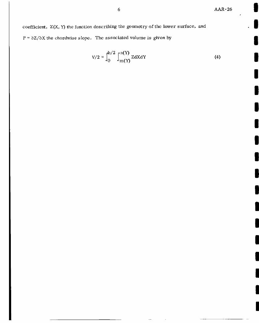
coefficient, Z(X, Y) the function describing the geometry of the lower surface, and

P 5 aZ/aX the chordwise slope. The associated volume is given by

7

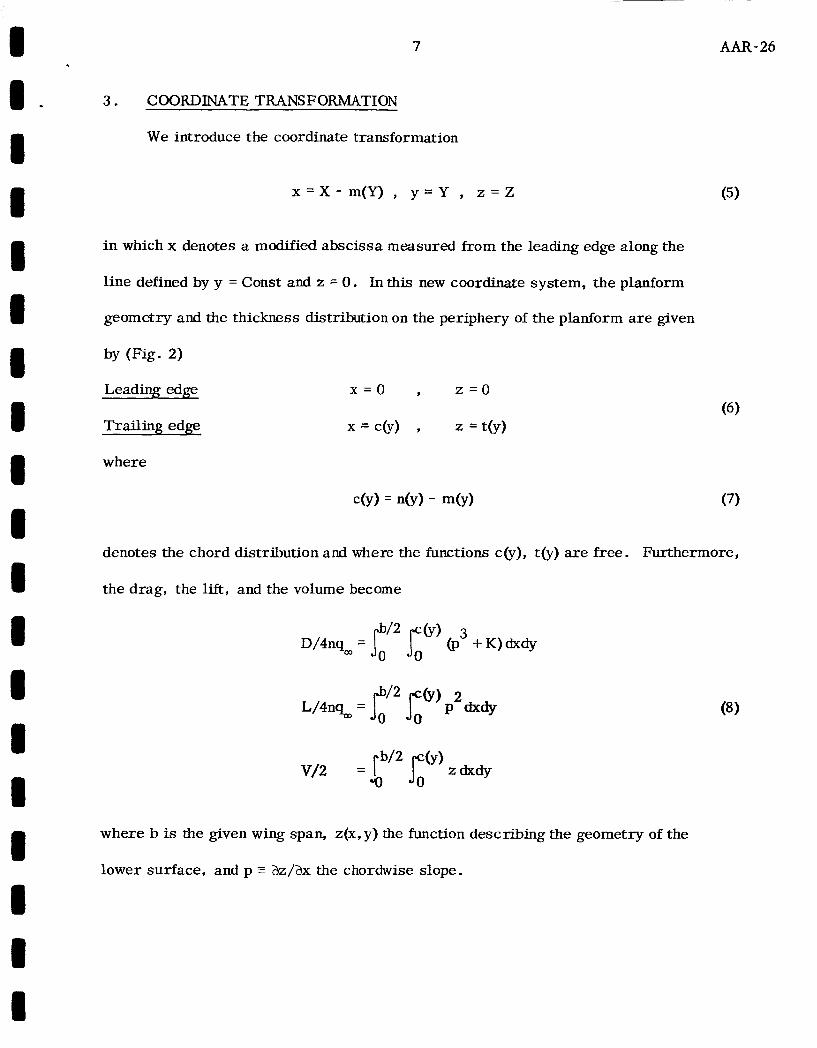
3 . COORDINATE TRANSFORMATION

We introduce the coordinate transformation

x = X - m ( Y ) , y = Y , z = Z

AAR- 26

i n which x denotes a modified abscissa measured from the leading edge along the

line defined by y = Const and z = 0. In this new coordinate system, the planform

geometry and the thickness distribution on the periphery of the planform are given

by (Fig. 2)

Leading edge

Trailing edge

where

x = o , z = o

x = c(y) 7 z = t(y)

denotes the chord distribution and where the functions COT), t(y) are free. Furthermore,

the drag, the lift, and the volume become

where b is the given wing span, ~(x, y) the function describing the geometry of the

lower surface, and p = &/ax the chordwise slope.

8 AAR- 26

4. MINIMUM DRAG PROBLEM

At this point, we formulate the following problem: "In the class of functions

z(x, y) which satisfy the isoperimetric constraints (8-2) and (8-3) as well as the boundary

conditions (6) , find that particular function which minimizes the integral (8- 1). " This is

a problem of the isoperimetric type with a variable boundary and involves the independent

variables x, y and the dependent variable z. According to Lagrange multiplier theory

(see, for instance, Chapter 3 of Ref. 5 ) , we study the minimization of the functional

form

subject to the constrains (8-2) and (8-3) as well as the boundary conditions (6) with the

understanding that the fundamental function is defined as

where X and X denote constant Lagrange multipliers. This fundamental function is

characterized by the first partial derivatives

1 2

2 F = 3 p -2h lp , F = O , F = X P q z 2

and the second partial derivatives

F = O zz , F = O , F = O ZP zq

in which p = az/ax and q = az/ay denote the chordwise slope and the spanwise slope

of the extrema1 surface.

9 AAR- 26

5. NECESSARY CONDITIONS 11 The function z(x, y) extremizing the integral (9) must be a solution of the Euler

equation I

aF /aX - Fz=O P

which, i n the light of Eqs . (11), can be rewritten as

Therefore, upon integrating in the x-direction, we see that the following first integral

is valid: c)

3ph - 2i1p - x x =f(y) 2

where f(y) is an arbitrary function of the spanwise coordinate.

The boundary conditions for the Euler equation are partly of the prescribed type

and partly of the natural type. The latter are to be determined from the transversality

condition

( F - p F ) 6 x - ( i F + q F ) b y + F 6 z = o P P P

(i denotes the derivative dx/dy evaluated on the boundary) which must be satLfied for

every set of variations consistent with the conditions imposed on the planform shape

and the th i chess distribution on the periphery of the planform. For the leading edge,

the following relations hold:

10 AAR- 26

(2 denotes the derivative dz/dy evaluated on the boundary) so that Eq. (16) is satisfied.

For the trailing edge, Eq. (16) is satisfied for every set of variations providing

F - p F = O , XF+qF = O , F = O P P P

that i s , providing

F=O , F = O (19) P

Because of Eqs. (10) and ( l l ) , the conditions (19) take the form

Trailing edge (20) 3 2 2

2 p + K - Alp + A t (y)=O , 3p - 2h lp=0

Once the solution of the Euler equation is obtained, it is necessary to verify that

it minimizes the functional (9). In this connection, the Legendre condition

F 2 0 PP

must be satisfied and ensures a relative minimum with respect to weak variations.

Because of Eq. (12-1), its explicit form is

3 p - x 2 0 1

If strong variations of the slope are considered, the Legendre condition is to be

replaced by the Weierstrass condition

where z and p are the ordinate and the slope of the extremal surface and p is the slope C

11 AAR-26

1. U I I 1 1 I U 1 I U U

1 I U U I

1

of the comparison surface. The explicit form of this inequality

2 bc - P) bC + 2P - X1) 2 0

must hold for every comparison slope consistent with the constraint

P, 20

which expresses the limit of validity of the Newtonian pressure law. Consequently,

the following inequality must be satisfied at each point of the extremal surface:

2p - x1 2 0

and is more restrictive than Ineq. (22).

12 AAR-26

6 . - NONDIMENSIONAL QUANTITIES

In order to simpllfy the representation of the results for the particular

cases, it is convenient to introduce the nondimensional coordinates

and the nondimensional chord distribution

Also, we define the thickness ratio of the root airfoil and the lift-to-drag ratio

7 =t(O)/c(O) , E = L/D

as well as the parameters

' I I I I I I I 1 I 1 I I I I I I I I

~~ ~

I I. I I I I

I I I I I 1 I I I

13

'i 1 . GIVENLIFT

If the lift is prescribed while the volume is free, the relationship X = 0 holds 2

s o that the extremal surface is described by the first integral

2 3p - 2x1p =f(y)

the fixed end conditions (6-1), and the natural boundary conditions

3 2 2 Trailing edge p f K - 1 ~ 1 G O , 3p -2X1p=0

Equations (32) admit the solutions

and

Trailing edge

3- X1 = 3 dK/4

3- p = d2K

AAR- 26

I I

I

(33)

(34)

indicating that the chordwise slope is constant over the trailing edge. E@ combining

Eqs. (31) and (32-2), we see that

meaning that the chordwise slope is also constant over the entire extremal surface. As

a consequence, the optimum wing is described by the partial differential equation

3 - P ' I h K

14 AAR- 26

which, in the light of the conditions (6-l), admits the particular integral

3- z = J 2 K x

Next, the conditions (6-2) are applied to obtain the relationship

(3 7)

meaning that the trailing edge thickness distribution and the chord distribution are

similar. Then, by forming the ratio of the above equations and introducing the

dimensionl, - 5 coordinates (27), we conclude that the optimum wing surface is given by

c = 5 (3 9)

Finally, the evaluation of the integrals (8) leads to

D = 6nKq bc(o) m

1

0 2 / 3 L = 2n(2K) q bc(o) ydq

co

s o that, because of Eqs . (30) and (38), the optimum wing is characterized by the

parameters

7, = 3Jz 3 - E, = ./4 / 3

1 c* =[2 $2 Jo Ydrl] - l

rl 2 JO

. I I I I I I 1 I I I I I I I I I I I

~

I 15 AAR-26

1 - Equations (41-1) and (41-2) show that the thickness ratio and the lift-to-drag ratio

of the extrema1 solution a re uniquely determined. On the other hand, Eqs. (41-3) and

(41-4) show that the chord distribution and the volume a re not uniquely determined;

in other words, there exist an infinite number of wings having the same maximum

value of the lift-to-drag ratio (41-2).

I

I I

I I I I I I I I I I 1 I 1 I

16 AAR- 26

8 . GIVEN LIFT AND VOLUME

If the lift and the volume are

first integral

given, the extremal solution is governed by the

0

3pL - 2x1p - x x = f(y) 2

the fixed end conditions (6-l), and the natural boundary conditions

3 2 2 2 p +K-X1p + x t ( y ) = O , 3p - 2 h l p = 0 Trailing edge

The analysis shows that these equations admit the following classes of solutions:

Class I x = o 2

Class I1 x 2 2 0

(43)

(44)

Solutions of Class I. For these solutions, which are characterized by X = 0, 2

Eqs. (42) and (43) reduce to Eqs. (31) and (32). A s a consequence, Eqs. (33) through

(41) are valid here. Once more, the thickness ratio and the lift-to-drag ratio are

uniquely determined while the chord distribution is not.

Iii order to determine the range of applicability of these solutions, we observe

that the volume-lift parameter V, is a known quantity. On the other hand, we can

formulate an auxiliary extremal problem, that of minimizing the right-hand side of

Eq. (41 -4) conceived as a product of powers of integrals subjected to the initial con-

dition y(0) = 1. If this is done and if the theory of Ref. 6 is applied, we see that the

extremum occurs for y = 1 and that the minimum value of the volume-lift parameter is

V, = 1/16. In the light of this result, we conclude that the solutions of Class I are

17

~

AAR-26

valid prodding

V, 2 1/16 (45)

Solutions of Class II. For these solutions, the natural boudary conditions (43)

can be solved in the form

Trailing edge P = (2/3)Xl tb) = (1/X2)(4X:/27 - K)

indicating that the chordwise slope and the thickness are constant along the trailing

edge.

If the first integral (42) is applied at the trailing edge and is combined with

Eq. (46-l), it is seen that

and that

2 3p - 2x1p 3. x (c - x) = 0 2

This is an algebraic equation of the second degree in p which--in the light of the Legendre

condition (22)--admits the solution

p = X1/3 + (1/3) [x: - 31 (c - x ) ] ~ ’ ~ 2

If this partial differential equation is integrated in the x-direction and the conditions

(6- 1) are imposed, we obtain the relationship

(49)

18

which, at the trailing edge, becomes

3/2 - 3- I1 1 t = (A1/3)c - (2/27X 2 ) r ( A L - 1 - 3X2c)

Since the trailing edge thickness is constant, Eq. (51) implies that the optimum wing

has a constant chord. Therefore, if the following definitions are introduced:

2 a = 31 C / h l 2

Eqs. (50) and (51) can be rewritten as

(54) 3

t = (A1 /27h2) G(1, a)

Consequently, in nondimensional form, the optimum shape is described by

1 The next step is to relate the quantity a to the prescribed values of the lift and

i the volume as well as to determine the scaling factors t and c . To do this, we combine

Eqs. (46-2) and (54-2) to obtain the relations

(53)

AAR- 26

.I I I I I I I I I I I I I I I B I I

(5 5)

I I

AAR-26

Furthermore, upon combining the shape equation (55) with the expressions (8) for

the drag, the lift, and the volume and introducing the following definitions:

A(u) = 2[4 - G(l,u)I-' (4 - 3a/2 + (2/5a) [ 6 - (6 - a)(l -

Nu) = 2[4 - G ( l , c ~ ) ] - ~ / ~ {2 - a/2 + (4/3u) [1 - (1 -

C(u) = [4 - G(1, a)]

+ 2

-1/3 - {1/2 - (2/15a2) [(2 +3u)(l - - 21)

we deduce that

D/nq bcK = A(u) (D

L/nq bcK2l3 = B(a)

V/bc K = C(u)

OD

2 1/3

so that

(57)

20

The final step consists of eliminating the quantity cx between Eqs . (55), (56-2),

and (59) to obtain the relationships

c = f,(L V,)

and

T,: = f2(V,) , c,: = f,(V,) , E , = f (V,) -- 4

which a r e plotted in Figs. 3 through 6 and are valid providing

v,: < - 1/16

Remark. In the previous analysis, it has been assumed that the span b is

prescribed. Should the span be free, all of the solutions would be of Class I and

would be characterized by the thickness ratio (41-1) and the lift-to-drag ratio (41-2).

AAR- 26

21 AAR-26

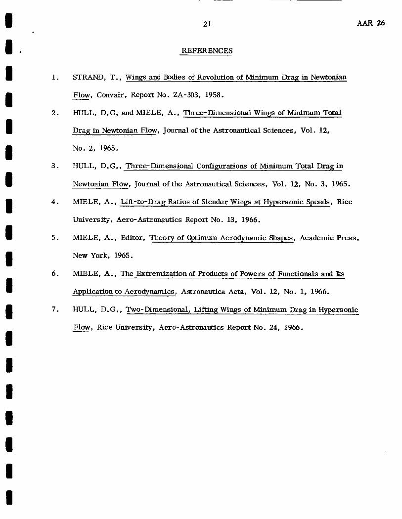
REFERENCES

1 . STRAND, T., Wings and Bodies of Revolution of Minimum Drag in Newtonian

- Flow, Convair, ReportNo. ZA-303, 1958.

HULL, D.G. and MIELE, A., Three-Dimensional Wings of Minimum Total

Drag in Newtonian Flow, Journal of the Astronautical Sciences, Vol. 12,

No. 2, 1965.

2 .

3. HULL, D. G., Three-Dimensional Configurations of Minimum Total Drag in

Newtonian Flow, Journal of the A s t r o ~ u t i c a l ScieIlces, Vol. 12, No. 3, 1%5.

4. MIELE, A., Lift-to-Drag Ratios of Slender Wings at Hypersonic Speeds, Rice

University, Aero-Astronautics Report No. 13, 1966.

5. MIELE, A., Editor, Theory of Optimum Aerodynam ic Shapes, Academic Press,

New York, 1965.

6 . MIELE, A., The Extremization of Products of Powers of Fuuctionals and Its

Application t o Aerodynam ics, Astronautica Acta, Vol. 12, No. 1, 1966.

7 . HULL, D.G., Two-Dimensional, Lifting Wings of Minimum DraginHypersonic

Flow, Rice University, Aero-Astronautics Report No. 24, 1966. -

22 AAR-26

Fig. 1

Fig. 2

Fig. 3

Fig. 4

Fig. 5

Fig. 6

LIST OF CAPTIONS

Coordinate system.

Planform geometry.

Optimum shape.

Optimum thickness ratio.

Optimum chord.

Maximum lift-to-drag ratio.

Y

Undisturbed

X

Fig. 1 Coordinate system.

Y

Fig. 2 Planform geometry.

1.00

0.75

0.50

0.25

6

4

5

2

0.2 C

Fig. 3

0.6 0.8 5 1

0 0

Optimum shape.

1 .o

0.02 0.04 0.06 0.08 v*

Fig. 4 Optimum thickness ratio.

0.1 0

Fig. 5 Optimum chord.

Fig. 6 Maximum lift-to-drag ratio.