m LAWFENCE UVERMORE LABORATORY

Wve^ctCatfomia/Vvmnore, CaMrofTK/^4550

UCRL- 51188

LINEAR POLARIZATION OF LOW-ENERGY BREMSSTRAHLUNG

Rober t W. Kuckuck (Ph.D. Thes i s )

MS. da te : F e b r u a r y 15, 1972

- N O T I C E -Thi» report was prepared as an account of work sponsored by the United States Government. Neither the United States nor the United States Atomic Energy Commission, nor any of their employees, nor any of their contractors, subcontractors, or their employees, nukes any warranty, express or implied, or assumes any legal liability o* responsibility for the accuracy, com­pleteness or usefulness of any information, apparatus, product or process disclosed, or represents that its use would not Infringe privately owned rights.

CONTENTS

A b s t r a c t v I. In t roduct ion 1

II. T h e o r y 2 A. C l a s s i c a l T r e a t m e n t of B r e m s s t r a h l u n g

P o l a r i z a t i o n . . . . . . . . . 2 B . Quantum Mechanica l T r e a t m e n t of

B r e m s s t r a h l u n g P o l a r i z a t i o n 6 EL P r e v i o u s Exper imen ta l Work . . . . . . 1 1 IV. E x p e r i m e n t 16

A. Appara tus 16 1. E l e c t r o n Source 19 2. Ta rge t C h a m b e r 21 3. T a r g e t s . . . . . . . . . 26 4 . P o l a r i m e t e r 28 5. X-Ray D e t e c t o r 35 6. E l ec t ron i c s System 35

B . P r o c e d u r e . . . . . 38 C. Expe r imen ta l Data 39 D. Data Analysis 39

1. Energy C a l i b r a t i o n of Mult ichannel Analyzer . . • 39

2. C o r r e c t i o n for Compton Sca t te r ing f rom the Ge(Li) De tec to r 41

3. C o r r e c t i o n for F l u o r e s c e n c e E s c a p e from the Ge{Li) Detector 41

4 . Removal of F l u o r e s c e n t L ines f r o m the Spec t rum 42

5. C o r r e c t i o n for the Compton P o l a r i m e t e r Energy R e s p o n s e 42

6. Norma l i za t ion of Spectrum (Dead -T ime C o r r e c t i o n s ) 43

7. Subtract ion of Backgrounds . . . . 43 8. Calcula t ion of t h e Difference of S p e c t r a . . 43 9. C o r r e c t i o n for A s y m m e t r y Rat io of

P o l a r i m e t e r 44 10. Fi t t ing a Po lynomia l to the F ina l

P o l a r i z a t i o n R e s u l t s . . . . • • 44

IV. Experiment (continued) E. E r r o r Analysis 44

V. Results 49 A. k-Dependence of Polarization 52 B. Z-Dependenee of Polarization 62 C. T n-Dependence of Polarization 68 D. 9-Dependence of Polarization . . . . . 68

VI. Comparison with Theory and Previous Experiments . . 73 A. Experimental Results of Motz and Placious . . 73 B. Gluckstern and Hull 's Calculation . . . . 78 C. Tseng and Pra t t ' s Calculation 78 D. Haug's Calculation 82 E. Sotnmerfeid's Theory . 8 2

1. Kirkpatrick and Wiedmann's Calculation . . 82 2. Kulenkampff, Scheer and Zei t ler ' s

Relativistic Transformation . . . . 9 0 VIL Conclusions 90

Suggestions for Future Work 92 Appendices:

A. Electron Energy Calibration 94 B. Ge(Li) Detector Efficiency Measurement . . . 97 C. Target Thickness Measurement by X-ray

Fluorescence Technique . . . . . 1 0 2 D. Polarimeter Asymmetry Ratio. Efficiency

and Energy Response 106 References 115

LINEAR POLARIZATION OF LOW-ENERGY BREMSSTRAHLUNG

ABSTRACT

The linear polarization of low-energy electron bremsstrahlung o

from thin targets (<50 /xg/cm ) of Al, Cu, Ag and Aa has been meas­ured for incident electron energies of 50, 75 and 100 keV. The polar­ization was measured as a function of photon energy at four emission angles (0 = 22.5°, 45°, 90° and 135°), using a Compton polarimeter with large asymmetry ratio (35 to 150) and a high-resolution Ge(Li) spectrometer (550 eV FWHM for 60-keV photons).

A brief discussion of the theoretical aspects of bremsstrahlung polarization, as well as a summary of calculational and experimental work to date, is presented. The Compton polarimeter is discussed in detail. The polarization data obtained here are compared with the predictions of various theories and, in particular, with the exact numerical bremsstrahlung calculation of Tseng and Prat t .

I. INTRODUCTION

An electron accelerated in the Coulomb field of an atomic nucleus radiates electromagnetic energy, called bremsstrahlung (braking radiation). Discovered by Roentgen in 1895, the phenomenon has been a subject of intense study throughout this century.^

Characteristics exhibited by bremsstrahlung include a continuous spectrum of photon energies from zero to the full kinetic energy of the electron, as well as linear and circular polarization. Linear polar­ization of low-energy electron bremsstrahlung is the subject of this investigation.

A photon beam is l inearly polarized when there is a preferential orientation in space of the electric vector. Linear polarization of bremsstrahlung is a function of the kinetic energy of the incident electron T Q , the energy of the emitted photon k, the angle of photon emission with respect to the direction of the incident electron B, and the atomic number of the target Z.

Most bremsstrahlung calculations apply to single electron inter­actions, and must be compared with experimental results obtained using very thin targets. To calculate the characterist ics of thick-target bremsstrahlung, complicated integration of the single interac­tion resul ts over successive electron collisions is necessary, a pro­cedure which has so far been unsatisfactory. The thin-target con­straint and the lack of a high-efficiency, high-resolution x-ray spectrometer have been the principal reasons for the paucity of quan­titative low-energy experimental results. However, the advent of the Ge(Li) detec.or provides an efficient, high-resolution x-ray spectrom­eter, and present-day thin-film technology allows preparation of targets thin enough to permit measurement using electrons of energy as low as 50 keV.

The purpose of this investigation was to apply these developments in measuring the linear polarization of thin-target, low-energy electron bremsstrahlung. The polarization was measured as a function of photon energy, electron energy, emission angle and atomic number.

A review of bremsstrahlung calculations and measurements is presented by Massey et al. in Ref. 1.

The electron energy range was between 50 and 100 keV. All other parameters were varied widely (Z = 13, 29, 47 and 79; 9 = 22.5°, 45°, 90° and 135°; and k = 0 to T.) to provide a broad sampling of the de­pendence of polarization upon them. The experimental results are compared with several calculations.

H. THEORY

A. Classical Treatment of Bremsstrahlung Folarization

Classical analysis of the bremsstrahlung phenomenon is instruc­tive since it is easily understood and illustrates many of the qualita­tive features of a more exact quantum mechanical treatment. Described classically, the accelerated electron is treated as a radiating electric dipole with components along each of the coordinate axes. Consider the geometry of Fig. 1. The radiation intensity observed at any point in space is the sum of intensities radiated from each of these three dipole components.

The radiation observed at a point in the x-z plane, at an angle 9 relative to the incident electron direction, can be broken into two linearly polarized intensity components, one parallel to the x-z plane, I.,, and one perpendicular to the plane, I . . Since radiation is linearly polarized in the direction of the dipole from which it emanated, it is clear that I, will consist only of radiation from the y-component dipole while I„ will consist of the sum of contributions from both the x- and z-component dipoles. Considering the angular distribution of the in-tensity of dipole radiation [i.(^) = I. sin $, where # is the angle between the jth dipole axis and the position vector at the point of observation] it can be seen that in the x-z plane

and

I ± = I y s in 2 90° = I (1)

I„ = I s in 2 9 + 1 s i n 2 (90° - 6). x z For an unpolarized electron beam there is axial symmetry so that I = I , and

I,. = I s in 2 9 + 1 c o s 2 9. (2) x y

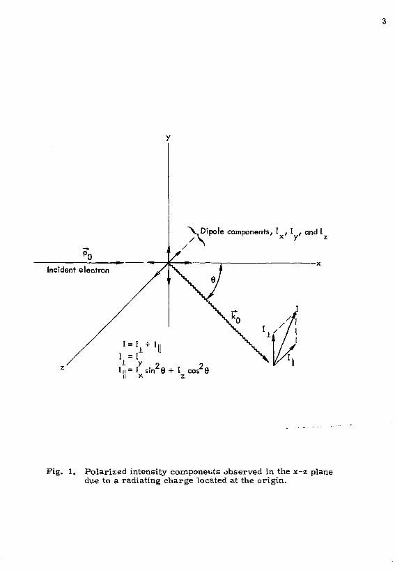
le components, 1 , 1 , and I

I = 1 J- y 2 2

I | i= I sin 6 + I cos 9

Fig. 1. Polarized intensity components observed in the x-z plane due to a radiating charge located at the origin.

If I.. ,- T the photons are linearly polarized. A measure of the polarization P(0) is defined as

P(<?) = T + f" • (3) 1 II

By this definition, the polarization P e n range from +1 (complete polarization perpendicular to the electron-photon plane) to -1 (complete polarization parallel to this plane).

Substituting the expressions for I and I. into Eq. (3) gives

P(0> = n x * * '- . (4) + 1 LA (2 esc2 8 - l)

It can be seen that the polarization can be predicted by calculating the two dipole component intensities, I and I .

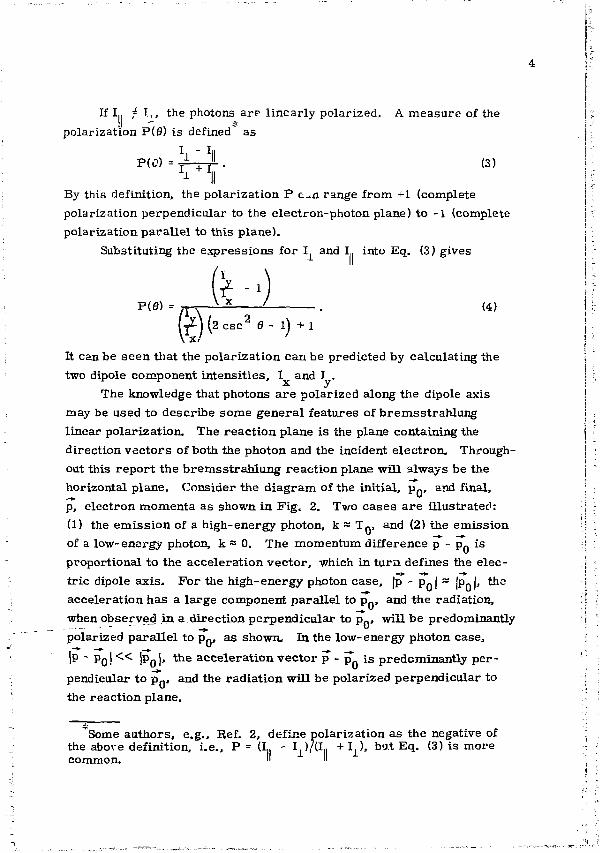
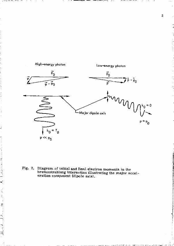
The knowledge that photons a re polarized along the dipole axis may be used to describe some general features of bremsstrahlung linear polarization. The reaction plane is the plane containing the direction vectors of both the photon and the incident electron. Through­out this report the bremsstrahlung reaction plane will always be the horizontal plane. Consider the diagram of the initial, p_, and final, p, electron momenta as shown in Fig. 2. Two cases are illustrated: (1) the emission of a high-energy photon, k ~ T Q , and (2) the emission of a low-energy photon, k ~ 0. The momentum difference p - p n is proportional to the acceleration vector, which in turn defines the elec­tric dipole axis. For the high-energy photon case, |p - p 0 | « [p |_, the acceleration has a large component parallel to p 0 , and the radiation, when observed in a direction perpendicular to p_, will be predominantly polarized parallel to p Q > as shown. In the low-energy photon case, |P - PQ j « | p 0 | , the acceleration vector p - p* is predominantly per­pendicular to p 0 , and the radiation will be polarized perpendicular to the reaction plane.

Some authors, e.g., Ref. 2, define polarization as the negative of the above definition, i.e., P = (I,. - I^/d,, + Ij_)» bu-t Eq. (3) is more common. " "

High-energy photon

P -PO

"l/|/|£ P~Pn

Fig. 2. Diagram of initial and final electron momenta in the bremsstrahlung interaction illustrating the major accel­eration component (dipole axis).

6

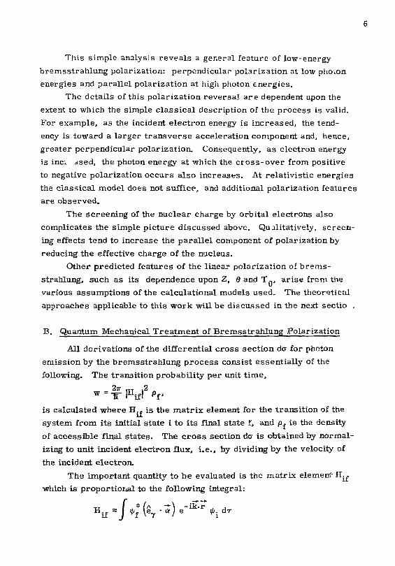
This simple analysis reveals a general feature of low-energy bremsstrahlung polarization: perpendicular polarization at low photon energies and parallel polarization at high photon energies.

The details of this polarization reversal a re dependent upon the extent to which the simple classical description of the process is valid. For example, as the incident electron energy is increased, the tend­ency is toward a larger t ransverse acceleration component and, hence, greater perpendicular polarization. Consequently, as electron energy is ine;. jsed, the photon energy at which the cross-over from positive to negative polarization occurs also increases. At relativistic energies the classical model does not suffice, and additional polarization features are observed.

The screening of the nuclear charge by orbital electrons also complicates the simple picture discussed above. Qualitatively, screen­ing effects tend to increase the parallel component of polarization by reducing the effective charge of the nucleus.

Other predicted features of the linear polarization of brents-strahlung, such as its dependence upon Z, 8 and T Q , ar ise from the various assumptions of the calculational models used. The theoretical approaches applicable to this work will be discussed in the next sectio .

B. Quantum Mechanical Treatment of Bremsstrahlung Polarization

All derivations of the differential cross section da for photon emission by the bremsstrahlung process consist essentially of the following. The transition probability per unit t ime,

w " TT l H if I p f * is calculated where H.„ is the matr ix element for the transition of the if system from its initial state i to its final state f, and p f is the density of accessible final states. The c ross section da is obtained by normal­izing to unit incident electron flux, i.e., by dividing by the velocity of the incident electron.

The important quantity to be evaluated is the matrix element H^ which is proportional to the following integral:

where e_, is the unit polarization vector of the photon and a is the Dirac matrix. The exponential results from expandhig the magnetic vector potential A, and ij,. and ip„ a re the Dirac wave functions for the initial and final states of the electron, respectively. Tc derive an "exact" cross section, it is necessary to use "exact" wave functions to describe the electron in the screened Coulomb field of the nucleus. It is not possible to solve the Dirac wave equation in closed form for an electron in a Coulomb field, pr imari ly because the wave function must be represented as an infinite se r i e s . ' However, various calcu­lations which expand the wave function in a partial wave ser ies and numerically solve the Dirac equation have been attempted. Also,

6 7 various approximate wave functions and procedures have been used. ' Bremsstrahlung cross-section calculations are relativistic or

nonrelativistic, depending upon whether the Dirac |H = ca . (p - eA) +j3mc + e<£f or Schroedinger {H = c[(p"- eA)

2 2 1/2 1 + m c ] ' + e<j>\ form of the Hamiltonian is used. Generally, one of three types of wave function is used, nonrelativistic Coulomb wave functions (Sommerfeld), relativistic Coulomb wave functions (Sommerfeld-Maue) or plane waves (Born approximation). Finally, various screening effects (atomic models) are considered.

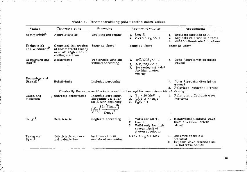
Table 1 summarizes the bremsstrahlung linear polarization calculations and their salient features.

A brief discussion of the calculations listed in Table 1 follows:

Sommerfeld's Theory o

Sommerfeld derived the matrix elements of the component di-poles in the bremsstrahlung process nonrelativistically, using the Schroedinger equation and assuming Coulomb wave functions. He assumed that the nuclear field is a pure Coulomb field, and that elec­tron spin could be ignored. Because he neglected screening, his theory is not valid for low electron energies, ~1 keV, or for high atomic numbers.

He considered the wave systems of an electron approaching a nucleus and departing in a new direction with reduced speed, the lost energy being emitted as a photon. The radiation emitted by the ac­celerated electron is composed of the intensity components, I , I

x y

T a b l e 1. B r e m s s t r a h l u n g p o l a r i z a t i o n c a l c u l a t i o n s .

Author C h a r a c t e r i s t i c s Screening Regions of validity Assumptions

Sommer fe ld 8

Kirkpatr ick and Wiedmann

Glucks te rn and HulllO

F ronsda l e and U b e r a l l 7

Olsen and Maxim on"

11 Haug

T s e n g and P r a t t 5

Nonrela t iv is t ic

Graphical integrat ion of Sommerfeld theory over all angles of r e ­coiling e lec t ron Relat iv is t ic

Rela t iv is t ic

Neglects sc reen ing

Same as above

Pe r fo rmed with and without sc reen ing

Includes sc reen ing

1. Neglects e lec t ron spin 2. Neglects re la t iv is t ic effects 3. Uses Coulomb wave functions Same as above

Born Approximation (plane waves)

(Basically the s ame as Glucks te rn and Hull E x t r e m e re la t iv i s t i c Includes sc reen ing .

1. Low Z 2. 0.06 << PQ « 1

Same as above

1. 2?rZ/137/3 0<< 1 2. 27rZ/1370<< 1 3. Screening not valid

for high photon energy

1. Born Approximation (plane waves)

2. Polar ized incident e ler t"ons except for more accura te screening) 1. T n > 20 MeV „ 1. Relat ivis t ic Coulomb wave

Screening valid for al l Z with accuracy :

(E/"V 2) / z y 2 lnf

Rela t iv is t ic

Rela t iv is t ic numer ­ical calculat ion

Neglects sc reen ing

E / m Q c

T 0 > 20 MeV p

2. T 0 , T , k » m„c 3 . P O 0 O = 1

1. Valid for all T Q

2. Low Z 3. Valid only for high

energy l imit of photon spec t rum

Includes var ious models of sc reening

5 keV < T r 1 MeV

functions

Relat ivis t ic Coulomb wave functions (Sommerfeld-Maue)

Assumes spher ica l potential Expands wave functions as par t i a l wave s e r i e s

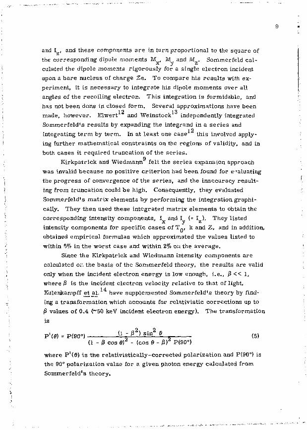
and I j and these components are in turn proportional to the square of the corresponding dipole moments M M and M . Sommerfeld cal-

x y z culated the dipole moments rigorously for a single electron incident upon a bare nucleus of charge Ze. To compare his resul ts with ex­periment, it is necessary to integrate his dipole moments over all angles of the recoiling electron. This integration is formidable, and has not been done in closed form. Several approximations have been made, however. Elwert and Weinstock u independently integrated Sommerfeld's results by expanding the integrand in a ser ies and

12 integrating t e r m by term. In at least one case this involved apply­ing further mathematical constraints on the regions of validity, and in both cases it required truncation of the ser ies .

g Kirkpatrick and Wiedmann felt the ser ies expansion approach

was invalid because no positive cri terion had been found for evaluating the progress of convergence of the ser ies , and the inaccuracy result­ing from truncation could be high. Consequently, they evaluated Sommerfeld's matrix elements by performing the integration graphi­cally. They then used these integrated matrix elements to obtain the corresponding intensity components, I and I (= I ). They listed

x y z intensity components for specific cases of T„, k and Z, and in addition, obtained empirical formulas which approximated the values listed to within 5% in the worst case and within 2% on the average.

Since the Kirkpatrick and Wiedmann intensity components are calculated or. the basis of the Sommerfeld theory, the results are valid only when the incident electron energy is low enough, i.e., £ << l, where £ is the incident electron velocity relative to that of light. Kulenkampff et al. have supplemented Sommerfeld's theory by find­ing a transformation which accounts for relativistic corrections up to /3 values of 0.4 (~50 keV incident electron energy). The transformation is P'(fl) = P(90°) (1 - £ 2 ) s i n 2 6 ( 5 )

d- /3 cos er - (cos e - pr POO°)

where P'(0) is the relativistically-corrected polarization and P(90°) is the 90° polarization value for a given photon energy calculated from Sommerfeld's theory.

To compare the results of the nonrelativistic and the "relativistically-corrected" Sommerfeld theory to measurements made in this investigation, a computer program was written to calculate nonrelativistic polarization using the Kirkpatrick and Wiedmann em­pirical formulas. "Relativistically-corrected" polarization was then calculated by applying Kulenkampff's transformation to the above. Comparisons are discussed in Section VI-E.

Calculation by Gluckstern and Hull 10 Gluckstern and Hull used the Born approximation to derive

relativistic cross sections for bremsstrahlung linear polarization. Their results are valid only under the conditions that 2JTZ/137 |3 0 << 1 and 2JTZ/I37)3 << 1 where /3_ and ft a r e the velocities of the incident and recoiling electron, respectively, relative to the velocity of light. This limits applicability to cases of low atomic number and j3 ~ 1. The calculations have been made with and without screening corrections but these corrections break down for the case of high-energy photon emission. Comparison is made with experimental results in Section VI-B.

Calculation by Haug

Haug haj relativistically calculated the linear polarization at the high-energy limit of the bremsstrahlung spectrum, using

15 Sommerfeld-Maue wave functions for the incident and recoiling electron. These wave functions behave asymptotically like a plane wave plus outgoing and ingoing spherical waves. The calculation is valid for all electron energies, and for low-Z elements. However, he calculates polarization for atomic numbers as high as 79. His results are compared to experiment in Section Vl-D. It is interesting to note that, contrary to the predictions of most theories, ' Haug finds that the linear polarization of bremsstrahlung depends upon the polarization state of the incident electron.

11

Calculation by Tseng and Prat t 5

Tseng and Pratt have calculated a relativistic bremsstrahlung cross section which is valid over an incident electron kinetic energy range of 5 keV to 1 MeV. The calculation assumes the atom to be a spherically-symmetric charge distribution of infinite mass , but alters the form of this charge distribution to include various models account­ing for screening. The incoming and outgoing electron wave functions are expanded in a partial wave ser ies and substituted into the Dirac equation which is then solved numerically. Matrix elements are then computed by numerical integration over these wave functions.

To date, Tseng and Prat t have published results pertaining only to differential bremsstrahlung cross sections integrated over all polar­ization states of the outgoing photons. However, their numerical technique readily predicts linear polarisation. Their computer pro­grams were obtained and modified for the Lawrence Livermore Laboratory's CDC 7600 computers. Results for specific cases of interest were calculated for comparison with measurement. Unfortu­nately, the computer time necessary to generate these results is very long, and therefore only a few representative cases have been calculated.

Other Calculations

Other calculations of bremsstrahlung polarization have been made but do not apply to the present work either because they merely confirm another, more complete, calculation or because they describe the bremsstrahlung process for much higher incident electron energies. They are referenced here only for completeness.

III. PREVIOUS EXPERIMENTAL WORK

Very few quantitative measurements of low-energy bremsstrahlung linear polarization have been accomplished to date. This is primarily because of the lack of an efficient high-resolution photon spectrometer. Also, thin targets were difficult to obtain until the last decade or so. The advent of the Ge(Li) detector in the late 1960's allows differential measurement of polarization as a function of photon energy from <5 keV to the bremsstrahlung endpoint energy.

The e a r l i e r m e a s u r e m e n t s (mos t ly t h i ck - t a rge t work) es tabl ished the fact that b r e m s s t r a h l u n g exhibi ts predominant ly p a r a l l e l po lar iza t ion . Some e x p e r i m e n t s showed qual i ta t ive a g r e e m e n t with s o m e a spec t s of

IV Sommerfe ld ' s t heo ry . The m o r e r e c e n t exper iment of Motz and 18 Plac ious is the only work which has provided enough data to allow

detailed c o m p a r i s o n s with theory . However , the scope of t h e i r ex­pe r imen t was l im i t ed . To date no s y s t e m a t i c inves t iga t ion of b r e m s ­s t rahlung p o l a r i z a t i o n as a function of incident e l e c t r o n ene rgy , t a rge t Z, photon e n e r g y and e m i s s i o n angle h a s been under taken .

A s u m m a r y of p rev ious e x p e r i m e n t a l work fol lows:

1905 19 Bark la , us ing the p o l a r i z a t i o n sens i t iv i ty of the Compton

sca t t e r ing p r o c e s s , m e a s u r e d the po l a r i z a t i on of x r a y s emi t ted at 90° to the e l e c t r o n b e a m from a t h i ck - t a rge t x - r a y tube . Hi s m e a s ­urement ave raged po la r i za t ion ove r the en t i re x - r a y e n e r g y spec t rum and showed a m e a n po la r i za t ion of 5% p a r a l l e l to the r e a c t i o n plane. The thick t a r g e t s and l a r g e d i m e n s i o n s of the s c a t t e r e r and de tec to r account for the low value of p o l a r i z a t i o n observed .

1909 20

B a s s l e r confi rmed that x r a y s w e r e po la r ized with t h e i r e l e c ­t r i c vector in the p lane of the inc ident e l e c t ron b e a m . He a l so con­cluded that the m e a n po la r i za t ion d e c r e a s e d as the e l e c t r o n energy was inc reased .

1910 20 21

B a s s l e r and Vegard showed tha t the ave rage po la r i za t ion was higher if the l o w e r - e n e r g y photons w e r e f i l tered out of the x - r a y spec t rum.

1923 22

Ki rkpa t r i ck used a b a l a n c e d - f i l t e r technique to o b s e r v e only those photons with ene rg i e s nea r the h igh-energy l imi t . He concluded

13

that for 58-keV incident electron e.iergy, the maximum polarization of the high-energy photons was only *0%.

1928 23

Ross also used a balanced-filter technique to measure polar­ization at the high-energy limit of the spectrum and obtained results which disagreed with Kirkpatrick's. Ross found the polarization of these photons to be 100%.

1928 24

Wagner and Ott attempted a measurement whici- was differ­ential in photon energy by analyzing the continuous spectrnm using a rock salt crystal . Their resul ts disagreed with both Ross ' and Kirkpatrick's In showing the high-energy polarization to be 47%. Targets of Fe. Cu, Ag and Pt were used, and no dependence upon atomic number was observed.

1IJ29 25

Duane performed the f irs t thin-target experiment. He bom­barded a Hg vapor target with 11.7-keV electrons and observed the x rays emitted at 90° to the beam. His measurements were not differ­ential in photon energy, and he found a mean polarization of 47% over the entire spectrum.

1929 og

Kulenkampff used targets that were thin relative to those of previous experimenters, but were sti l l thick in an absolute sense. For electron energy of 38 keV, he found the mean polarization over the entire spectrum to be 45%, in agreement with Duane's results . Further­more, using a balanced-filter technique, he observed 100% polarization at the high-energy limit.

1930 27 Dasannacharya, using electrons of energy ~40 keV, measured

the mean polarization of the entire x-ray spectrum from thick targets

14

as a function of target thickness. His targets ranged from 25 n to 6 cm in thickness, all thick by absolute standards. The results indi­cated an exponential rise in polarization as target thickness decreased. A maximum polarization of 48% was observed. The shape of the polarization versus target thickness curve was independent of electron energy.

1934 17 Cheng used the balanced-filter technique to observe the x rays

emitted from thick targets of Al, Cu, and W when bombarded by elec­trons of energies between 20 and 100 keV. He used filter combinations of Mo-Nb, Pd-Rh and W-Ta to measure polarization at 19.5, 23.8 and 68.5 keV, respectively. The major result of this experiment was the determination that, for a given x-ray energy, the polarization in­creased as the atomic number of the target decreased.

1936 28 Piston used a balanced-filter technique to investigate the

polarization of 68.5-keV photons from Al and Ag targets of 19 and 2

0.2 mg/cm thickness, respectively. Incident electron energy was varied up to 102 keV. For T- ~ 70 keV, he observed complete polar­ization near the high-energy limit of the spectrum.

1941 29 Boardman, using targets of Ni, Ag and Pb with thicknesses o of the order of 10 mg/cm , performed an experiment s imilar to

Piston's and obtained the same resu l t s .

1954 30 Kulenkampff et al. measured bremsstrahlung polarization by

observing the directions and ranges of the recoiling photoelectrons wh^n the bremsstrahlung was absorbed in a cloud chamber. Unfor­tunately, poor statistics resulted in very large experimental uncertainty.

1

1956 31 Motz used a Nal(Tl) spectrometer to measure polarization,

differential in photon energy, for 1.0-MeV elect 'ons incident on a 2 2

1 mg/cm thick Al target and a 0.4 mg/cm Au target. His results showed qualitative agreement with the predictions of the Born ap­proximation calculation by Gluckstern and Hull.

1958 32 Motz and Placious used the technique of Motz to measure the

polarization at the high-energy limit as a function of bremsstrahlung emission angle. The incident electron energy was 500 keV and the

2 2 targets were 4.3 mg/cm of Be and 0.21 mg/cm of Au. The results again showed qualitative agreement with the Gluckstern-Hull predictions.

1960 1 R

Motz and Placious summarized the theoretical calculations to that date. They also published experimental results of the polariza­tion at the high-energy limit of the photon spectrum for T_ = 50 and 100 keV and for targets of Be and Au. Their results were again com­pared with the Gluckstern-Hull calculations. The theory predicted too large a value of polarization, particularly at small forward angles.

1961 33 Kulenkampff and Zinn measured the polarization of x rays

emitted at 90° from low-Z targets bombarded with electrons of ~35 keV. The measurement was differential in photon energy, and the results

Q

showed qualitative agreement with predictions of Sommerfeld.

1964

Huffman measured the- polarization of bremsstrahlung from a Hg vapor target as a function of incident electron energy, photon energy and angle of emission. The electron energies were 10, 15, 20, 25 and 30 keV. His results were compared with the predictions of

Sommerfeld, corrected for relativistic effects. The agreement be­tween theory and experiment was quite poor.

1968 35 Scheer et. aL. measured polarization as a function of photon

energy and emission angle for 50-keV electrons on carbon. They also measured the polarization as a function of photon energy at an angle of 20° for 180-keV electrons incident on AUOo and Au. They show reasonable agreement with the predictions of Fronsdal and Uberall . 7

1970

Slivinsky was the first experimenter to use high-resolution Ge(Li) and Si(Li) spectrometers to measure bremsstrahlung polari­zation. He measured the polarization of the x rays emitted by com-merical x-ray machines (thick targets) . He could not determine the polarization at the high-energy limit, but did show that polarization increases rapidly for high photon energies. He also observed a de­crease in polarization with increasing electron energy.

IV. EXPERIMENT

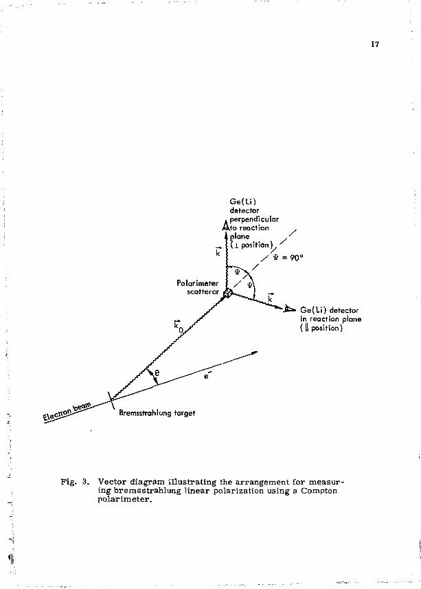
The experiment performed here measured the bremsstrahlung polarization, as defined in Eq. (3), using a Compton polarimeter, as illustrated in Fig. 3. A detailed discussion of the technique follows.

A. Apparatus

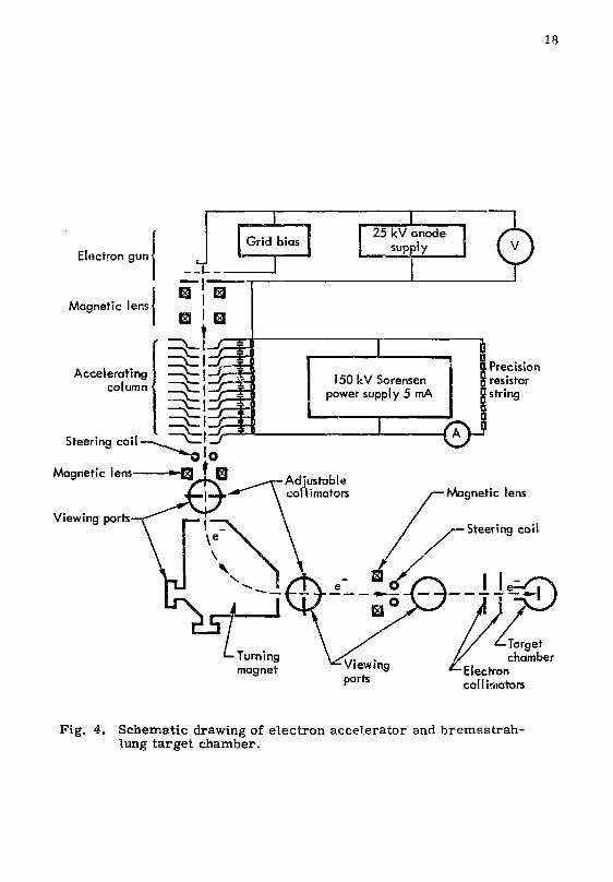
The experimental apparatus consisted of: (1) a source of elec­trons, (2) a target chamber, (3) a thin target, (4) an x-ray polarim­eter employing a Ge(Li) detector, and (5) electronics for monitoring the electron beam and acquiring polarization data. Figure 4 is a schematic drawing of the accelerator and target.

17

Ge(Li) detector

. perpendicular A to reaction i plane ,

( j . position]\y / * = 90°

/

/

-fc» Ge(Li) detector in reaction plane (II position)

Bremsstrahlung target

Pig. 3. Vector diagram illustrating the arrangement for measur­ing bremsstrahlung linear polarization using a Compton polarimeter.

18

Electron gun

Magnetic lens

Accelerating column

Steering co i l -

Grid bias 25 kV anode J

supply I V

0 J U

^£=¥3 150 kV Sorensen

power supply 5 mA

Precision resistor string

t Magnetic lens * H 3 ! B

Viewing ports—<r"""^ _ _

-Adjustable animators Magnetic lens

Steering coii

• Turning magnet Viewing

ports

-Target chamber

•Electron collimators

Fig. 4. Schematic drawing of electron accelerator and bremsstrah-lung target chamber.

1

1. Electron Source

The following accelerator characterist ics were necessary to accomplish this experiment: (1) well-defined beam energy, (2) sufficient beam current to establish reasonable bremsstrahlung intensities, and (3) sufficiently small beam diameter and divergence at the target. A source having some of these features was the LLL Statitron accelerator which provided a subnanosecond burst of electrons for detector im­pulse response studies. The accelerator was dismantled, moved to a new location, and rebuilt with many modifications to make it appro­priate for this work. Presently, the accelerator is capable of deliver­ing a steady-state current of 50 JUA with energies ranging from a few keV to 125 keV. The beam diameter is not larger than 0.5 cm at the target. Electron energy is known to within ±250 eV (see Appendix A) and is stable to within 0.2%. Many characterist ics of this accelerator

37 have been described in detail by Lasher, but a summary of the steady-state capability is in order here (refer to Fig. 4).

Electron Gun—A new electron gun was mounted on the acceler­ator for this work. This was necessary because the guns used in the pulsed mode are extremely expensive and were very sensitive to changing high-vacuum conditions encountered in the early stages of this experiment.

The gun used is a model EE-55 electron tube. It consists of a planar, tungsten dispenser- cathode and grid assembly, and is rated for a pulsed current delivery of several amperes. The oun was designed for short electron paths in a planar geometry, and had to be modified to deliver enough current to the target 2 meters away. The modification consisted of attaching a bell-shaped electrode to the gun to focus the electrons and sllow passage to the accelerating column through an aperture in the gun anode. Without this addition to the gun, the beam current on target was insufficient to perform the experiment.

A voltage of up to 30 kV can be maintained across the electron gun. Beam current is controlled by varying the cathode heater power or the grid voltage.

Manufactured by Machlett Laboratories, Inc.

2

Accelerator — Upon exit from the gun, the electrons are focused by two magnetic lenses. They are then accelerated in a 12-electrode

37 linear accelerating column described by Lasner. The voltage across the column is provided by a well-filtered, high-voltage supply with output capability of 0 to 150 kV at 5 mA. Voltage ripple is less than 0.01% (15 V at maximum output).

The kinetic energy of the electrons is the sum of the voltages on the electron gun and the accelerating column. The maximum vari­ation in this energy is less than 0.2%. This stability is evidenced by the sharp endpoint energies obtained in bremsstrahlung spectra taken over very long time intervals, as seen in Fig. A-1 of Appendix A

A clean environment was needed to avoid poisoning the cathode by hydrocarbons from O-rings and organic pump fluids. Consequently, metal gaskets were used wherever possible, and the system was initially evacuated with cryopumps. A Vaclon pump evacuated the sys-

_7 tem to base pressure of approximately 10 Torr . Operating pres-

—fi sure was typically 2 X 10 Torr or l ess .

Focusing and Momentum Analysis — In its previous location, the accelerator produced a beam of electrons that could only be used in the vertical direction. To provide a horizontal beam and allow adequate space for this experiment, and also to maintain energy stability, an analyzing magnet was added. The magnet was designed to bend a beam of 175-keV electrons through 90° with a 20-cm radius of curva­ture. This required a field strength of 76 gauss.

To avoid the large, cumbersome coil and pole pieces necessary if the magnet were mounted outside the beam pipe, the magnet was designed with the pole pieces themselves serving as vacuum bar r ie r s . Further, the design provided for a viewing port to allow visual obser­vation along the horizontal beam axis (see Fig. 4). A simple degauss­ing circuit was built to eliminate hysteresis effects and obtain r e ­producible magnetic fields.

Fositionable Al collimators with beveled edges were placed im­mediately before and after the analyzing magnet. They were mounted on a vacuum-tight metal bellows arrangement that allowed external adjustment without disturbing the vacu';*n. The surfaces of the

collimators were painted with a phosphor (Z;i_SiO.Mn) to permit ob­servation of the beam position and spot size through the three ac­celerator viewing ports. These ports were covered with Pb-loaded glass. Additional fixed Al collimators were located nearer the target chamber.

Two additional focusing magnets were required to obtain the desired beam spot size on target (see Fig. 4). All beam pipes were wrapped with magnetic shielding to reduce the effect of the earth's magnetic field on the beam trajectory. Without this shielding it was impossible to deliver the beam to the target chamber.

2. Target Chamber

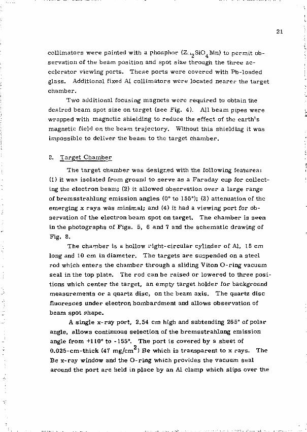
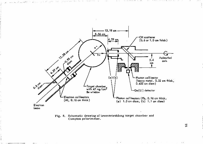
The target chamber was designed with the following features: (1) it was isolated from ground to serve as a Faraday cup for collect­ing the electron beam; (2) it allowed observation over a large range of bremsstrahlung emission angles (0° to 155°); (3) attenuation of the emerging x rays was minimal; and (4) it had a viewing port for ob­servation of the electron beam spot on target. The chamber is seen in the photographs of Figs. 5, 6 and 7 and the schematic drawing of Fig. 8.

The chamber is a hollow right-circular cylinder of Al, 15 cm long and 10 cm in diameter. The targets are suspended on a steel rod which enters the chamber through a sliding Viton O-ring vacuum seal in the top plate. The rod can be raised or lowered to three posi­tions which center the target, an empty target holder for background measurements or a quartz disc, on the beam axis. The quartz disc fluoresces under electron bombardment and allows observation of beam spot shape.

A single x-ray port, 2.54 cm high and subtending 265° of polar angle, allows continuous selection of the bremsstrahlung emission angle from +110° to -155°. The port is covered by a sheet of

2 0.025-cm-thick (47 mg/cm ) Be which is transparent to x rays. The Be x-ray window and the O-ring which provides the vacuum seal around the port are held in place by an Al clamp which slips over the

22

Fig. 5. Experimental setup showing electron accelerator, target chamber, and Compton po'iarimeter.

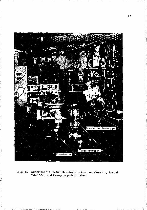
23

Fig. 6. Compton polarimeter in position to observe bremsstrahlung emitted at 22.5° with the Ge(Li) detector positioned perpen­dicular to the bremsstrahlung reaction plane.

I

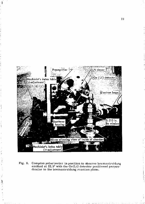
24

Fig. 7. Compton polarimeter in position to observe bremsstrahlung emitted at 13 5°, with the GefLi) detector positioned in the bremsstrahlung reaction plane. Polarimeter is partially disassembled to show scat terer .

Electron beam

CH scatterer (0 .6 or 1.0 cm thick)

'Electron collimators (A! , 0.16cm thick)

Photon collimator (heavy metal, 0.32 cm thick, 0.635 cm diam)

Ge(Li ) detector

Photon collimators (Pb, 0.16 cm thick, (a ) 1.3 cm diam, (b) 1.1 cm diam)

Fig. 8. Schematic drawing of bremsstrahlung target chamber and Compton polarimeter.

U l

26

chamber (Fig. 7). The electron beam penetrates the targets , but is totally absorbed in the Be window of the chamber.

The chamber has two lucite viewing ports sealed with O-rings. One is a 0.64-cm-diam opening located at the vertical center of the chamber wall at +140°. The other is a 5-cm-diam opening in the bottom of the chamber and a mi r ro r must be used to observe the target through this window (see Fig. 6).

The chamber is electrically isolated from the accelerator beam pipe (ground) by a Teflon spacer and Teflon bolt sleeves. It is isolated from the polarimeter table (ground) by a lucite cylinder which also supports the chamber from beneath.

Data runs were normalized to equal amounts of beam charge col­lected by the target chamber. Therefore, in addition to maintaining a high electrical impedance to ground, it was also necessary to insure that there was no low-energy secondary electron current collected by the chamber. This was accomplished by biasing the chamber at -90 V with respect to the accelerator beam pipe. The electrical isolation

p was adequate to maintain an impedance to ground of >5 X 10 Q and assure accurate current measurement.

The system was designed for the chamber to be pumped by the vacuum pumps on the accelerator. However, a valve was located on the drift tube to allow isolation of the chamber so that targets could be changed without bringing the accelerator to atmospheric pressure.

3. Targets

The major cri terion for targets used in this study was that they be thin enough to minimize electron scattering effects. Four target materials were selected: A1(Z = 13), Cu(Z = 29), Ag(Z= 47) and Au(Z = 79), so that the dependence of polarization upon Z could be studied.

They were prepared by vacuum evaporation onto Parylene sub-o

strates between 500 and 1000 A thick. Uniformity across tha foil was

Parylene is the name given to a Poly-para-xylyene produced by Union Carbide. It is a CH, chain with a structure [CH2-< > ~ ^ H 2 ] n

where n « 5 X 10 3 .

27

insured by mainta in ing a l a r g e d i s t ance between the evaporation, source and s u b s t r a t e during the evapora t ion .

Foi l t h i cknes s was d e t e r m i n e d in two ways . F i r s t , dur ing evap­orat ion, the m a s s deposited on the s u b s t r a t e was mon i to red by s imu l ­taneous depos i t ion onto a d i sc of known a r e a mounted adjacent to the foil. The weight of this d i sc was m e a s u r e d dur ing evapora t ion with a Cahn m i c r o b a l a n c e . Difficulties in applying th i s method dur ing the ear ly s t ages of the work r e s u l t e d in l a r g e unce r t a in t i e s (±30%) in t a rge t t h i c k n e s s . La te r r e f i n e m e n t s in technique y ie lded foil th ick­ness va lues a c c u r a t e to wi thin ±10%.

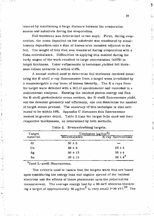
A second method used to d e t e r m i n e foil t h i cknes s involved m e a s ­uring the K- she l l x - r a y f l uo re scence from a t a r g e t when i r rad ia ted by a monoenerge t ic x - r a y b e a m of known intensi ty. The K x r a y s from the t a rge t w e r e detected with a Si(Li) s p e c t r o m e t e r and r e c o r d e d in a mult ichannel ana lyze r . Knowing the incident photon e n e r g y and flux, the K-she l l pho toe l ec t r i c c r o s s s ec t ion , the K-she l l f luo rescence yield, and the d e t e c t o r g e o m e t r y and efficiency, one can d e t e r m i n e the number of t a rge t a t o m s p r e s e n t . The a c c u r a c y of th is t echn ique is a l so e s t i ­mated to be wi th in 10%. Appendix C d i s c u s s e s t h i s f luorescence method in g r e a t e r detai l . Tab le 2 l i s t s the t a r g e t foils used qnd the i r r e spec t ive t h i c k n e s s e s , as d e t e r m i n e d by both m e t h o d s .

Table 2. B r e m s s t r a h l u n g t a r g e t s .

T a r g e t Th icknes s Qjg/cm2) m a t e r i a l Mic roba l ance X - r a y f luorescence

Al 50 ± 5 — Cu 50 ± 5 52 ± 5 Ag 50 ± 15 38 ± 4 Au 50 ± 1 5 3 8 ± 4 a

Used L - s h e l l f luorescence .

The c r i t e r i a used to i n s u r e tha t the t a r g e t s w e r e th in a r e based upon cons ide r ing the energy l o s s and angular sp r ead of the incident e lec t rons and the effects of t h e s e phenomena upon the po la r i za t ion m e a s u r e m e n t . The average ene rgy los t by a 50-keV e l e c t r o n t r a v e r s -ing a t a r g e t of approx imate ly 50 fig/cm is very s m a l l (~20 eV). The

28

effect of the angular spread due to elastic scattering of the electrons in the target can be estimated by calculating the mean scattering angle and comparing it to the finite angular resolution of the polarim-eter. The average number of elastic scattering events an electron of energy TQ (keV) experiences in t ravers ing a target of thickness pxing/cm ) and atomic number and mass Z and A, respectively, is

39 given by

For the 12 combinations of energies and targets used, the typical value of N was between 2 and 2.5. The minimum number (best case) was 1.7 for 100-keV electrons on Al, and the maximum number (worst case) was 4 for 50-keV electrons on Au.

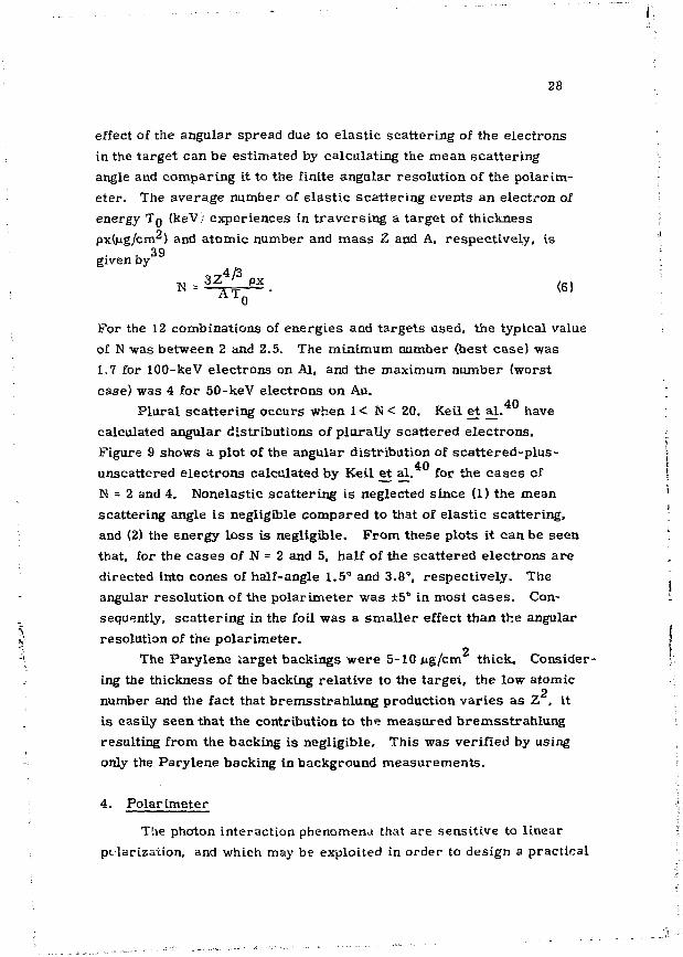
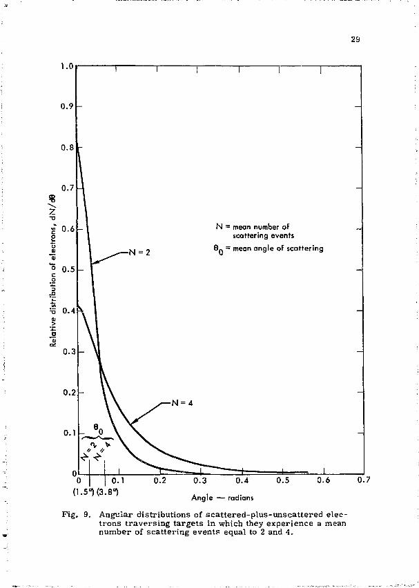
40 Plural scattering occurs when 1< N < 20. Keil et al . have calculated angular distributions of plurally scattered electrons. Figure 9 shows a plot of the angular distribution of scattered-plus -

40 unscattered electrons calculated by Keil et al. for the cases of N = 2 and 4. Nonelastic scattering is neglected since (1) the mean scattering angle is negligible compared to that of elastic scattering, and (2) the energy loss is negligible. From these plots it can be seen that, for the cases of N = 2 and 5, half of the scattered electrons are directed into cones of half-angle 1.5" and 3.8°, respectively. The angular resolution of the polarimeter was ±5° in most cases . Con­sequently, scattering in the foil was a smaller effect than the angular resolution of the polarimeter.

2 The Parylene iarget backings were 5-10/ug/cm thick. Consider

ing the thickness of the backing relative to the target, the low atomic 2

number and the fact that bremsstrahlung production varies as Z , it is easily seen that the contribution to the measured bremsstrahlung resulting from the backing is negligible. This was verified by using only the Parylene backing in background measurements.

4. Polarimeter

The photon interaction phenomena that are sensitive to linear polarization, and which may be exploited in order to design a practical

29

1.0

0.9

0.8 -

-N = 2

N = mean number of scattering events

G 0 = mean angle of scattering

(1.5°) (3.8°) 0-3 0.4

Angle — radians

0.5 0.6 0.7

Fig. 9. Angular distributions of scattered-plus-unscattered elec­trons traversing targets in which they experience a mean number of scattering events equal to 2 and 4.

30

p o l a r i m e t e r , a r e the pho toe lec t r i c effect, photodis in tegra t ion of the deuteron, p a i r product ion, Compton sca t t e r ing , and photofission.

41 They a re t r e a t e d in rev iews by F a g g and Hanna and McCallum and 42 Verv ie r . Detai led cons ide ra t ion of these phenomena r e v e a l s that

significant advantages can be obtained using the Compton sca t t e r ing p r o c e s s at m e d i u m and low photon ene rg i e s (k = <1 MeV).

P o l a r i z a t i o n Sensitivity of Compton S c a t t e r i n g — T h e sensi t iv i ty of the Compton s c a t t e r i n g p r o c e s s to b r e m s s t r a h l u n g po la r i za t ion is easi ly s een f r o m the Kle in-Nishina formula for the d i f ferent ia l c r o s s

43 sect ion, 2

dg(<ft) a4$te4-"^»-'*)-2 2

where r n = e An^c is the c l a s s i c a l r ad iu s of the e l ec t ron , ip is the angle through which the incident photon is s ca t t e r ed , df2 is the e lement of solid angle into which it is s c a t t e r e d , q> is the angle be tween the e l ec t r i c vec to r of the incident photon and the s c a t t e r i n g p lane (defined as the plane containing both the incident and s c a t t e r e d photon), and k_ and k a r e the ene rg i e s of the incident and s c a t t e r e d photon, r e s p e c ­t ively. In the above, the c r o s s s e c t i o n has been in t eg ra t ed over all

2 po la r iza t ion s t a t e s of the s c a t t e r e d photon. It is s e e n tha t the cos <p t e r m is the p o l a r i z a t i o n - s e n s i t i v e p a r t of the c r o s s sec t ion , and r e s u l t s in a m a x i m u m for $ = it 12 and a min imum for <t> = 0.

The in i t ia l and final photon e n e r g i e s a r e r e l a t ed by the exp re s s ion

k = ._° . (8) 1 + 9 _ (i - cos ijj)

m Q c

n

When k f l < < m Q c , k « k Q ; and in Eq . (7), the t e r m k / k Q + k Q / k is approximate ly 2. F o r ij/ = ir/2, t he c r o s s sec t ion then b e c o m e s

This impl ies an ideal r e s p o n s e to po la r i za t ion at low e n e r g i e s , i.e.. a finite c r o s s s ec t ion for <j> = ir/2 and z e r o c r o s s s e c t i o n for <t> = 0. For values of 0 o ther than v/2, t h i s ideal r e s p o n s e is degraded .

31

A measure of the sensitivity of a Compton scatterer to polariza­tion is expressed by the asymmetry ratio R, defined as

o = da (j. = TT/2) R ~ da (I = 0) • ( 1 0 )

For the ideal, low-energy case, R — °o. However, as the incident photon energy k Q increases, R decreases and its maximum occurs at ip < 7r/2. Consequently, for a given k_ there is an angle ip~ for which R is a maximum. For energies ii: the range up to 100 keV, k/k + k / k deviates from the value 2 by less than 1.5%. Therefore, for these energies R is a maximum near <p = itj2.

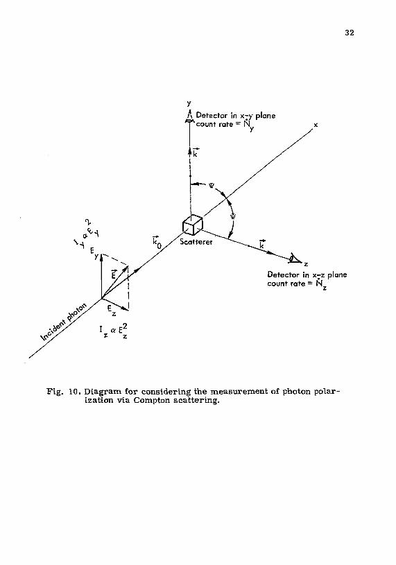
Now assume a beam Df x rays, linearly polarized in some arbi­t ra ry plane, to be incident upon a sca t terer as indicated in Fig. 10. The total intensity of this beam may be divided into two components, I (<x E j and I Ice E J, whose polarizations lie in orthogonal planes. If the detector is alternately positioned in the x-y and x-z planes, as shown, different counting rates will, in general, be observed. The difference of these ra tes , divided by their sum, is related to the x-ray polarization through the asymmetry ratio, R.

Let N and N be the counting ra tes observed with the detector in the x-z and j:-y planes, respectively. Also let d0(O) and dcr(?r/2) be the Klein-Nishina differential cross section for $ = 0 and $ = ir/'2, respectively, where <j> is the angle between the electric vector of the x-ray component and the scattering plane.

It is then seen that the counting rate observed by the detector in the x-z plane results from fractions of both components of the incident beam scattering into it, i.e.,

N z = I z da(O) + I d<T(jr/2). (11)

We have assumed ideal geometry and 100% detector efficiency. Similarly,

N = I da(7i72) +1 da(O). 0.2) y z ' y

32

v

i\ Detector in x-y plane

Scatterer

^ ^ . Detector in x-z plane count rate = N_

I aEz

z z

Fig. 10. Diagram for considering the measurement of photon polar­ization via Compton scattering.

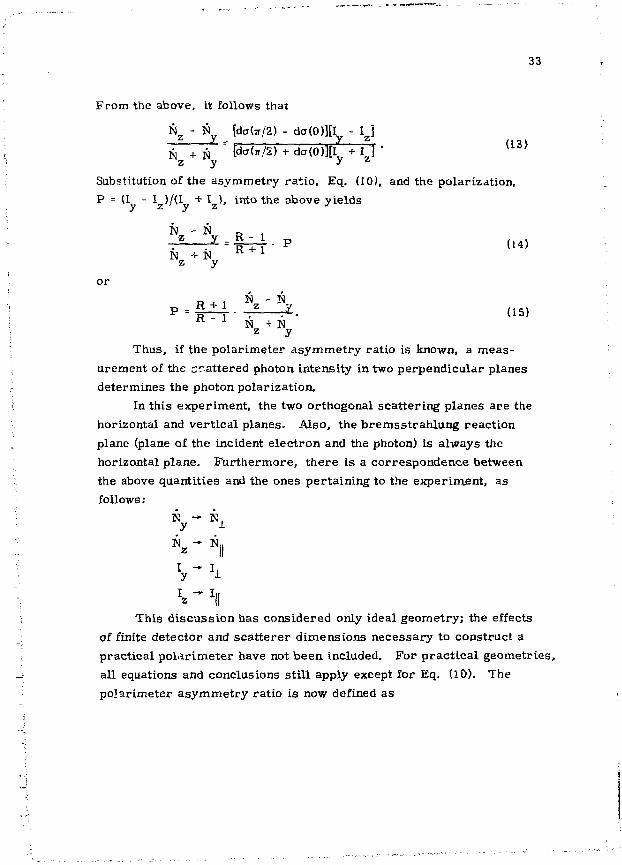
33

From the above, it follows that

N z - N y [dcr(7r/2) - da(0)][Iy - I z j N + N = (d<x<ir/2) + da(0)][I, + I J " U 3 >

z y y z

Substitution of the asymmetry ratio, Eq. (10), and the polarization, P = (I - I )/(I + I ), into the above yields y z y z

(14) TV - N

z y -+ N

R - 1 R + l

P

% y

P = R + 1 N -z N .7

R - 1 N + N z y

(15)

Thus, if the polarimeter asymmetry ratio is known, a meas­urement of the scattered photon intensity in two perpendicular planes determines the photon polarization.

In this experiment, the two orthogonal scattering planes are the horizontal and vertical planes. Also, the bremsstrahlung reaction plane (plane of the incident electron and the photon) is always the horizontal plane. Furthermore, there is a correspondence between the above quantities and the ones pertaining to the experiment, as follows:

y J-

\ ~ \\ This discussion has considered only ideal geometry; the effects

of finite detector and scatterer dimensions necessary to construct a practical pol.irimeter have not been included. For practical geometries, all equations and conclusions still apply except for Eq. (10). The polarimeter asymmetry ratio is now defined as

34

/ . e<V^)^<k 0 . * , 9 )

R(kQ) 3 A<bA^

dfi

/

*i*lL e f k g . ^ ^ ^ f k g . ^ p )

&4M

(16) dfi

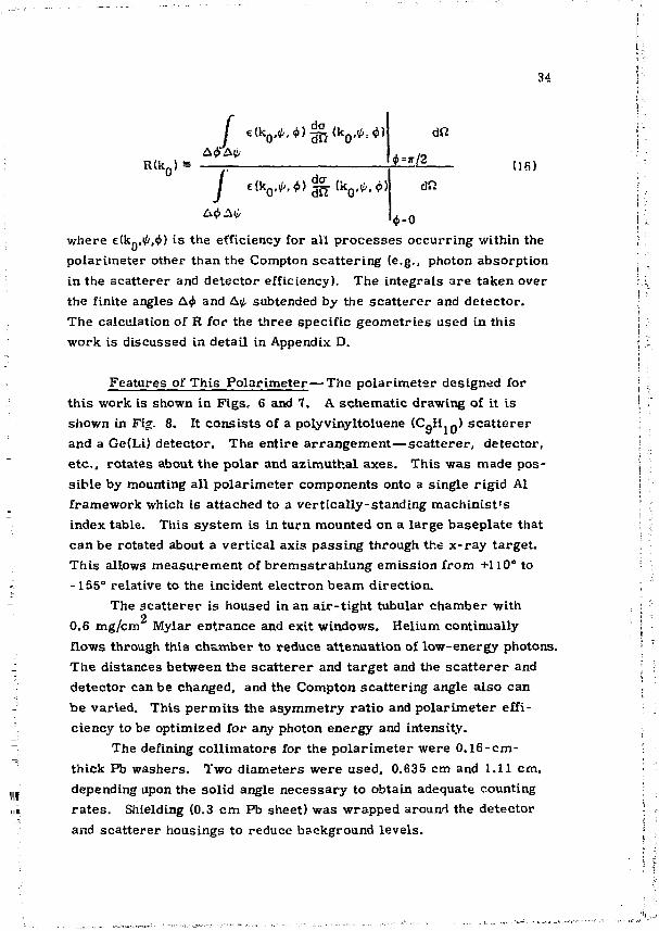
$-0 where e(k0,^,<fi) is the efficiency for all processes occurring within the polarimeter other than the Compton scattering (e.g., photon absorption in the scatterer and detector efficiency). The integrals a re taken over the finite angles A^ and A(i. subtended by the scat terer and detector. The calculation of R for the three specific geometries used in this work is discussed in detail in Appendix D.

Features of This Polarimeter—The polarimeter designed for this work is shown in Figs. 6 and 7. A schematic drawing of it is shown in Fig. 8. It consists of a polyvinyltoluene (CQH.Q) sca t terer and a Ge(Li) detector. The entire arrangement—scatterer , detector, etc . , rotates about the polar and azimuthal axes. This was made pos­sible by mounting all polarimeter components onto a single rigid Al framework which is attached to a vertically-standing machinist 's index table. This system is in turn mounted on a large baseplate that can be rotated about a vertical axis passing through the x-ray target. This allows measurement of bremsstrahlung emission from +110° to -155° relative to the incident electron beam direction.

The scat terer is housed in an air- t ight tubular chamber with 2

0.6 mg/cm Mylar entrance and exit windows. Helium continually flows through this chamber to reduce attenuation of low-energy photons The distances between the scat terer and target and the sca t te rer and detector can be changed, and the Compton scattering angle also can be varied. This permits the asymmetry ra t io and polarimeter effi­ciency to be optimized for any photon energy and intensity.

The defining collimators for the polarimeter were 0.16-cm-thick Pb washers. Two diameters were used, 0.635 cm and 1.11 cm, depending upon the solid angle necessary to obtain adequate counting ra tes . Shielding (0.3 cm Pb sheet) was wrapped around the detector and scatterer housings to reduce background levels.

35

The scat terer for a low-energy Compton polarimeter should be of low atomic number to reduce photoelectric absorption of the inci­dent and scattered photons. It should also be amorphous to eliminate the possibility of coherent interference phenomena perturbing the scattering. Organic hydrocarbons generally satisfy these cri teria.

The scat terer for this polarimeter was machined from a commercially-available organic scintillator.^ Two sca t te rers of different thicknesses, 0.6 Cm and 1.0 cm, were used. For low-Z targets, at high energy, the 1-cm sca t te rer was needed to obtain a reasonable count ra te .

Three combinations of collimation and scatterer thickness were used. The asymmetry ratio (also the efficiency and energy response) was calculated for all three cases using a computer program described in Appendix D. Asymmetry ratios varied from 35 to 200.

5. X-Ray Detector

The x-ray detector used in the polarimeter was a planar-type Ge(Li) detector having an active area of 0.95 cm X 0.95 cm and a depletion depth of 1.02 cm. When biased with 2500 V, it exhibited a

241 resolution of ~550 eV for the 59.5-keV y ray from Am. The de-o

tector was mounted in vacuum behind a 12 mg/cm Be window and was cooled by a cold finger extending from a dewar of liquid nitrogen. A 0.635-cm-diam collimator was positioned in front of the detector, just outside of the Be vacuum window.

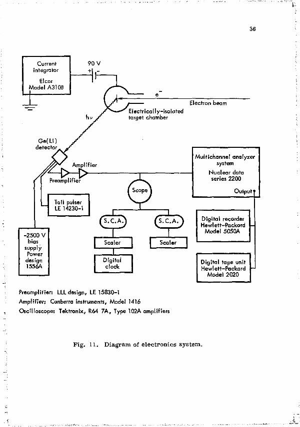
6. Electronics System

Standard nuclear counting techniques and electronic circuits were used for recording data. A diagram of the overall electronics system is shown in Fig. 11.

Electron Energy Measurement—The electron energy was mon­itored by observing voltages applied both to the electron gun and to —5

Composition of the scintillator was 97.5% polyvinyltoluene (CgH 1 0 ) and 2.5% terphenyl ( C l 8 H 1 4 > .

36

Current integrator

El cor Model A310B

Electron beam Electrically-isolated target chamber

Ge(L i ) detector

Amplif ier

Preamplifier

Tail pulser LE 14230-1

X S.C.A

-2500 V bias

supply Power

design 1556A

S.C.A

Scaler ] t Scaler

Digital clock

Preamplifier: LLL design, LE 15830-1

Ampli f ier: Canberra instruments, Model 1416

Oscilloscope: Tektronix, R64 7A , Type 102A amplifiers

Multichannel analyzer system

Nuclear data series 2200

Output

Digi tal recorder Hewlett-Packard

Model 5050A

Digital tape unit Hewlett-Packard

Model 2020

Pig. 11. Diagram of electronics system.

37

the accelerating column. The electron gun voltage was measured with a 0-60 kV electrostatic voltmeter. The voltage applied to the accelerating column was determined by measuring -he current through a resistor string in the power supply. These instruments were cali­brated by determining the bremsstrahlung endpoint energy with the Ge(Li) spectrometer (see Appendix A).

Beam Current Integration—The electron beam current collected by the target chamber was integrated by a commerically-available current integrator (Elcor, Model A310B). The integrator was equipped with a built-in calibration unit, and its calibration was checked every few hours. The procedure consisted of driving a full-scale current through the indicator and integration circuits via a mercury cell for a fixed time. The total measured charge was compared to the product of the full-scale current and the t ime. Manual meter and circuit ad­justments were made until th? above comparison differed by less than 0.5%. Occasionally, the built-in calibration unit was shown to be oper­ating properly by connecting an external dry cell and precision resistor to the input of the integrator.

Amplifiers—The preamplifier was an LLL design employing a two-stage, cooled FET. It was housed immediately adjacent to the detector with its FET inside the detector vacuum system.

The linear amplifier was made by Canberra Instruments (Model 1416). Pulse shaping of 2 jusec was used to match the optimum input needs of the Nuclear Data multichannel analyzer.

Scalers—Two single-channel analyzers were used with scalers to monitor interesting x-ray energy intervals during successive runs. This provided an easy method for adjusting beam current to obtain proper counting ra tes , and also provided a running check of the over­all progress of the experiment. For example, broken foils were im­mediately detected by a sharp drop in the scaler counting rate. In addition, rea l time measured by a digital clock triggered by the scalers was compared with the live time recorded in the multichannel analyzer to make dead-time corrections to the data.

38

Multichannel Analyzer—The multichannel analyzer was a Nuclear Data, Series 2200, 4096 channel analyzer system. Individual data runs were stored in separate quarters of the memory (1024 channels), allow­ing for informative comparisons by overlaying one upon another and displaying the result on a CRT. This was particularly useful in check­ing for gain shifts by overlaying the characterist ic peaks observed in each of two runs, or for accelerator energy shifts by overlaying the high-energy endpoint of the bremsstrahlung spectrum,

B. Procedure

Each experimental run was conducted in the following manner: The accelerator was set at the proper energy and the beam spot size was observed, using the quartz disc in the target chamber. The bremsstrahlung target was then inserted into the beam, and the cur­rent was adjusted to provide an optimum detector counting rate . Beam current was never allowed to exceed 10 juA since a higher current would destroy the target.

With the detector in the horizontal (reaction) plane, data were recorded until a given amount of charge was collected by the Faraday cup (target chamber). The target was replaced by a background target, or empty target holder, and the process was repeated for a background measurement. With the accelerator off, the Ge(Li) detector and elec­tronics system were calibrated using monoenergetic x rays from

'Am and Co sources. The detector was then rotated to the verti­cal plane ar.d the signal, background, and calibration runs were re ­peated. A total of 192 accelerator runs were necessary, each lasting from 20 to 200 min.

The data were recorded in approximately 500 of the 1024 channels available in one-quarter of the memory of the multichannel analyzer. After four runs, they were transferred onto magnetic tape for reading into a CDC 6600 computer. In addition, the data were printed on paper tape, and the CRT display was photographed for cursory exami­nation of the progress of the experiment.

39

C. Experimental Data

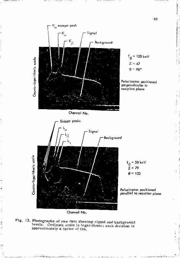
Photographs of raw data displayed on a CRT using a logarithmic ordinate scale are shown in Fig. 12 to illustrate typical signal-to-background levels encountered. The background count ra te was higher for T« = 100 keV than for lower electron energies, but always less than 4% of signal levels. Apparent from these photographs is the sharpness of the high-energy end point of the spectrum, a feature which allows measurement of polarization even as the value of k / T 0 approaches unity, and the high resolution of the characteristic x-ray lines from the target, a feature which allows accurate removal of these lines from the spectrum.

D. Data Analysis

A program was written for use with a CDC 6600 digital computer to reduce the raw data. The operations performed by the program are listed in sequence below:

1. Energy calibration of multichannel analyzer. 2. Correction of spectrum for Compton scattering from Ge(Li)

detectcr. 3. Correction of spectrum for fluorescent escape from Ge(Li)

detector. 4. Removal of target fluorescent lines from the spectrum. 5. Correction for Compton polarimeter energy response. 6. Normalization of spectrum (dead-time corrections). 7. Subtraction of backgrounds. 8. Calculation of the ratio of the difference and sum of perpen­

dicular and parallel spectra , (N. - N I)/(N.. + N^). 9. Calculation of final polarization oy correcting the above for

asymmetry ratio of the polarimcter. 10. Fitting of polynomial to final polarization resul ts .

These operations will now be discussed in detail.

1. Energy Calibration of Multichannel Analyzer

The Ge(Li) detector and associated electronics system was calibrated using standard IAEA radiation sources of Am and Co.

40

Channel No .

Escape peaks

Background

50keV '0 Z = 79

0 = 135

Polarimeter positioned parallel to reaction plane

Channel No .

Fig. 12. Photographs of raw data showing signal and background levels. Ordinate scale is logarithmic: each division is approximately a factor of ten.

41

These sources provided photons of energies 11.9, 13.9, 17.8, 20.8, 26.348, 59.543, 121.97 and 136.33 keV. The computer program selects the largest peaks in the calibration spectrum, fits these peaks with gaussian line shapes, and determines the centroid channel. It then assigns the appropriate ene.-oy to that channel and a straight line is fit to the resulting points using a least- squares technique. This line becomes the energy-versus-channel calibration for the run. A separate calibration was made for each run.

2. Correction for Compton Scattering from the Ge(Li) Detector

When rnonoenergetic photons are incident upon a Ge(Li) detector, A certain fraction will be absorbed via the photoelectric effect while another, smaller, fraction will be scatterc-d out of the detector, depositing a portion of the photon energy in the crystal. The result is that counts appear in low-energy channel*, rather than in the higher, full-vnergy channel associated with the photopeak.

44 This effect has been measured by Slivinsky and calculated by Smith for a detector geometry similar to the one used here . Their results ->vere applied to correct the present data to energies as low as 2 keV. The magnitude of the correction is a few percent or less in all cases, anrl affects only the low-energy channels where k < T n / 4 .

3. Correction for Fluorescence Escape from the Ge(Li) Detector

Most of the Ge K x rays produced in the detector via photoelec­t r i c interactions of the incident x rays will be reabsorbed. Some will escape, however, and carry away approximately 10 keV of energy (K = 9.976 keV and Ka = 10.984 keV). The result of this phenomenon or p ^ is the occurrence of two peaks in the pulse-height spectrum approxi­mately 10 keV below the photopeak. Actually, these peaks are un­resolved in the upectrum and appear as a single "escape peak." The magnitude of this "escape peak" relative to the photopeak is a function of incident photon energy, and was experimentally measured in the deterr nation of detector efficiency described in Appendix B. Figure B-3 shows a plot of th° escape-peak-to-photopeak ratio as a function of energy.

42

The program makes a channel-by-channel correction for the escape peak, starting at the high-energy end of the spectrum and working downward, ising the measured escape-peak-to-photopeak ratio as a function of energy. The correction is negligible for energies above 50 keV, is small between 15 and 50 keV because the spectrum shape is decreasing with increasing energy, but can reach values of from 10 to 50% at energies below 10 keV.

4. Removal of Fluorescent Lines from the Spectrum

The characterist ic x rays of the bremsstrahlung target are un-polarized and it is necessary to remove these lines from the spectrum. We attempted to interpolate betveen the bremsstrahlung counts on each side of the lines, leaving a continuous spectrum. Th? uncertainty in this interpolation, however, was significant. Therefore, all data within the energy intervals of the characterist ic lines were discarded and the final polarization in this region was obtained from interpola­tion of the polarization in other regions of the spectrum. To do this, the program sets the counts in all channels within the specified interval to zero. This is done after the corrections for Compton scattering and Ge K x-ray escape are made.

5. Correction for the Compton Polarimeter Energy Response

The energy response of the Compton polarimeter was calculated, and is discussed in detail in Appendix D. The polarimeter has two effects upon the bremsstrahlung spectrum. The first is to shift the photon energv due to the Compton scattering according to Eq. (8). The second is to broaden the photon energy due to the finite dimen­sions of the scat terer and detector.

It is seen in the Appendix that the width of the energy response function is small enough to allow correction of the scattered energy spectrum, to obtain the unscattered spectrum, simply by applying Eq. (8). This is accomplished by multiplying k by the ratio k n /k . Of course, the ratio k_/k is not a linear function of energy, and therefore the multiplication is not done channel-by-channel. The width of each energy interval must be adjusted by the derivative of k

43

with respect to k,.. The program makes this nonlinear multiplication correction to the scattered .spectrum to obtain the true bremsstrahlung spectrum incident upon the polarimeter.

6. Normalization of Spectrum (Dead-Time Corrections)

-All spectra are normalized to the same total incident beam charge and corrected for analyzer dead-time by multiplying the counts in each channel by a constant. This normalization constant i?

% T K = - ^ x i (17)

where Q n = some arbi t rary reference charge to which each run was

normalized, Q = total integrated beam current incident on target, T = actual elapased time of run, T = total analyzer "live time" during run.

The dead-time contribution to the normalization n : s always <0.2%.

7. Subtraction of Backgrounds

Background data undergo the same corrections as signal data, and are then subtracted from the signal plus background data channel by channel.

8. Calculation of the Difference of Spectra

The corrected spectra are then combined, channel by channel, to form the following rat io:

N,. - N, N + N ±

where N,. are the corrected counts corresponding to the polarimeter detector lying in the reaction plane, and N. are the corrected counts corresponding to the polarimetcr detector perpendicular to the reac­tion plane.

44

9. Correction for Asymmetry Ratio of the Polarimeter

The asymmetry ratio R of the polarimeter is a function of photon energy. This asymmetry ratio affects the apparent photon polarization, and as was discussed in Section IV-A-4, is used as a correction to the recorded data in the following manner:

F(k) - NH " N l R ( k ? + l (18) ^ W N +Nj_ R(k) - 1 U 8 ;

where P is the polarization, N. and N„ are the corrected counts, and R(k) is the asymmetry ratio of the polarimeter, all for energy k. This correction is applied channel by channel.

Three diffei-ent polarimeter geometries were employed during the course of these measurements, and the asymmetry ratio for each is plotted as a function of photon energy in Appendix D. It is seen that R is large enough for all three cases, so that the correction (R + 1)/ R - 1) ranges between 1.06 and 1.01. For ease in applying this cor­rection in the computer program, each of the three asymmetry ratios were approximated by the straight lines indicated in Pig. D-4. The largest error in the correction ratio (R + 1)/(R - 1), resulting from this approximation is less than 0.3%, and the typical e r ror is <0.1%.

10. Fitting a Polynomial to the Final Polarization Results

The data analysis program plots polarization P as a function of photon energy k for a given target material , electron energy, and angle of emission. These data are fit to polynomials of degree I through 4 using a standard least-squares technique. The value of X-square divided by the number of degrees of freedom is then com­puted as a measure of the goodness of each fit.

E. Er ror Analysis

The polarization P is defined as a ratio of intensity components of the bremsstrahlung, i.e.,

P = p — J L . (10)

45

However, as de r ived from e x p e r i m e n t a l data, the p o l a r i z a t i o n is

N„ - N 1 - R + 1 . . i (20)

N l l + N l R

or P = N • K • f (21)

where N = (N„ - N )/N„ + Nf) and N. and N„ a r e counts in a p a r t i c u l a r energy in terva l ; K = (R + 1)/(R - 1) is the p o l a r i m e t e r a s y m m e t r y co r ­r ec t i on factor; R is the p o l a r i m e t e r a s y m m e t r y r a t i o ; and f is the r a t io of the t rue p o l a r i z a t i o n to the value of the polynomial fit (f equals unity for a perfect fit to the data).

The to ta l uncer ta in ty , A P , in t h e po la r i za t ion is g iven by

where AN, AK and Af a r e the individual unce r t a in t i e s in the fac tors of Eq. (21). Each of t h e s e unce r t a in t i e s wi l l now be d i s c u s s e d sepa ra t e ly .

A_K_

The p o l a r i m e t e r a s y m m e t r y c o r r e c t i o n K = (R + 1)/(R - 1) is a function otily of the a s y m m e t r y r a t i o R. Consequently, the uncer ta in ty AK is due solely to the uncer ta in ty AR, and the dependence is given by

AK = | | • AR = 2 A R

? (23) 8 R ( R - l T

and

,'AK \ 2 / j A R V (24)

The uncertainty in R is est imated at <25%. The ratio R was cal­culated as described in Appendix D, and no experimental verification of this was poss ib le . However, experimental verif ication of another feature of the polarimeter predicted by the same calculation (shape of the energy response function to monoenergetic, unpolarized photons) gave confidence that a 25% uncertainty in asymmetry ratio is conservative.

46

Since the correction factor K is small (<6% in the worst case), a large uncertainty in R still yields a small uncertainty in final polar­ization. For example, the 25% uncertainty in R results in an e r ro r in the polarization of <2% for R = 35 (the worst case).

Af

The uncertainty Af is a measure of the quality of the polynomial fit to the final polarization data. The magnitude of this uncertainty is obtained as a numerical by-product of the least-squares calculation. Implicit in Af are the uncertainties due to counting statistics for both the signal and background spectra, as well as uncertainties due to the fit itself. Values for Af/f are typically about 1%, but in cases of ex­tremely poor statistics, such as obtained at the endpoints of the spec­t rum at backward angles, or in cases of near-zero polarization (N, » N,| ) the uncertainty is as large as 15%.

AN

The uncertainty AN results from the uncertainties in N. and N.., the measured and corrected counts at each energy. Since N. and N.. a re independent quantities.

o r

AN = 2 N ± N H - fl-^j +[-*rM (26)

where N., N.., AN., AN,, and, consequently, AN, are functions of the II _ . H photon energy. Furthermore,

/AN\2 4 N f a ! W^i (27)

47

The uncertainties which contribute to N do so through the terms AN. and AN i.e., AN^ = £ ( A N ^ and ARj = £ (AN.,)[. A discussion of

each of these contributions (AN.), and (ANn)., follows.

Electron Energy

The accelerator voltage was determined to 1.1% and was stable to<0.2%. Since polarization varies slowly with electron energy, r e ­sulting uncertainty is negligible.

Target Thickness

The uncertainty in target thickness is estimated at<10%. How­ever, the discussion in Section IV-3 establishes that the targets used here were sufficiently thin to have no effect upon polarization. This conclusion was based upon comparing the small mean angle of elec­tron scattering in the target to the la rger angular spread of the polarimeter.

33 Kulenkampff and Zinn measured polarization as a function of target thickness and extrapolated to zero thickness to obtain true polarization. Their results, if applicable to this work, indicate that a correction of 5% should be made to the present d^'a for the worst case (T-. = 50 keV, Z = 79). However, since their measurements were made only for Au at 90° and also were strongly a function of polarimeter geometry, it is not clear to what extent their corrections apply here. Consequently, no correction to the data was made, but a systematic uncertainty of between zero and 2% has been estimated based on their findings.

Bremsstrahlung Emission Angle

The uncertainty in determining the bremsstrahlung emission angle 0 is negligible. The spread in 0, AS, was accounted for in the calculation of the polarimeter asymmetry ratio, but still has the effect of averaging the bremsstrahlung polarization over its extent. The A0 subtended by the polarimeter was 7° or 10°, depending upon the par­ticular collimator used. Since polarization varies slowly and smoothly over this small angular spread, the e r ro r is <1.5%. This was

48

estimated using the shape of the angular dependence of polarization as calculated by Tseng and Pratt .

Polarimeter Azimuthal Angle

The uncertainty in the azimuthal angle, <j>, is negligible and its spread, A<£, is accounted for in the calculation of polarimeter asym­metry ratio.

Beam Current Integration

The accuracy of the current integrator is ±2%. However, only its precision affects the uncertainty of the polarization since the meas­ured value of integrated current is used to normalize one run against another; the absolute value is of no consequence. The precision of the integrator was continually checked by integration of a known, cur­rent for a fixed time. The variations were <0.5% of the mean value.

Dead-Time Corrections

Dead-time corrections are always <0.2%. The uncertainty in this correction is negligible.

Ge(Li) Detector Efficiency

The absolute efficiency of the Ge(Li) detector was measured (Appendix B) and is believed accurate to within ±3%. However, the ratio (N,. - N. )/(N,, + N^) is independent of detector efficiency, and so this uncertainty has no effect upon polarization.

Fluorescence Escape Correction

The uncertainty in the fluorescence escape peak correction is <10% at high energies (50 keV), where the correction is small, and considerably less at low energies (15 keV), where the correction be­comes significant. At 5 keV, where the correction to the counts can be as large as 50% the resulting uncertainty in polarization is still <5%.

49

Correction for Escape of Compton-Seattered Photons

The uncertainty in this correction can be as large as 50% at low energies. Since the magnitude of the correction is <2%, the consequent uncertainty in the polarization ranges from negligible to <2% at a few keV.

Polarimeter Energy Response

The effect of the energy response of the polarimeter is to shift and broaden the apparent energy of the incident photons. The final data are corrected for the shift. The broadening was shown to be negligible by examining the line shapes of fluorescent x rays observed by the polarim­eter. Therefore, no correction was applied to the data for this effect.

The magnitudes of AK/k, Af/f and AN/N were calculated for various cases and substituted into Eq. (22) to obtain the final uncertainty in the polarization. This uncertainty, AP/P, is indicated as e r r o r bars on some of the data points. Error bars have only been calculated for representa­tive ^ases.

V. RESULTS

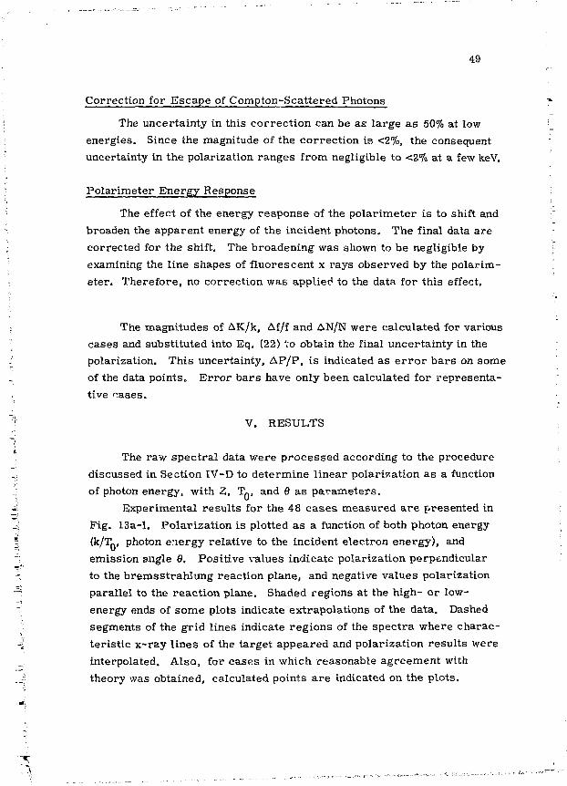
The raw spectral data were processed according to the procedure discussed in Section IV-D to determine linear polarization as a function of photon energy, with Z, TQ , and 8 as parameters .

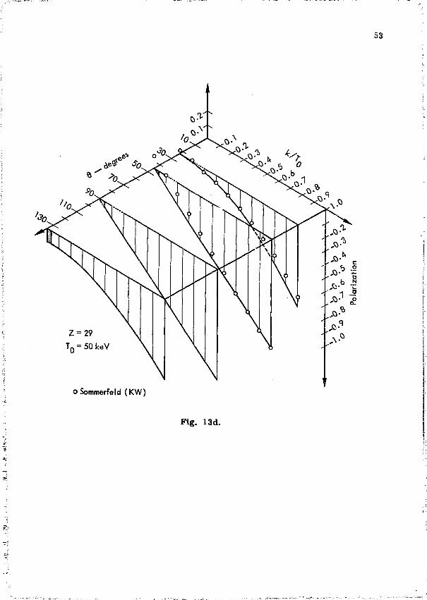
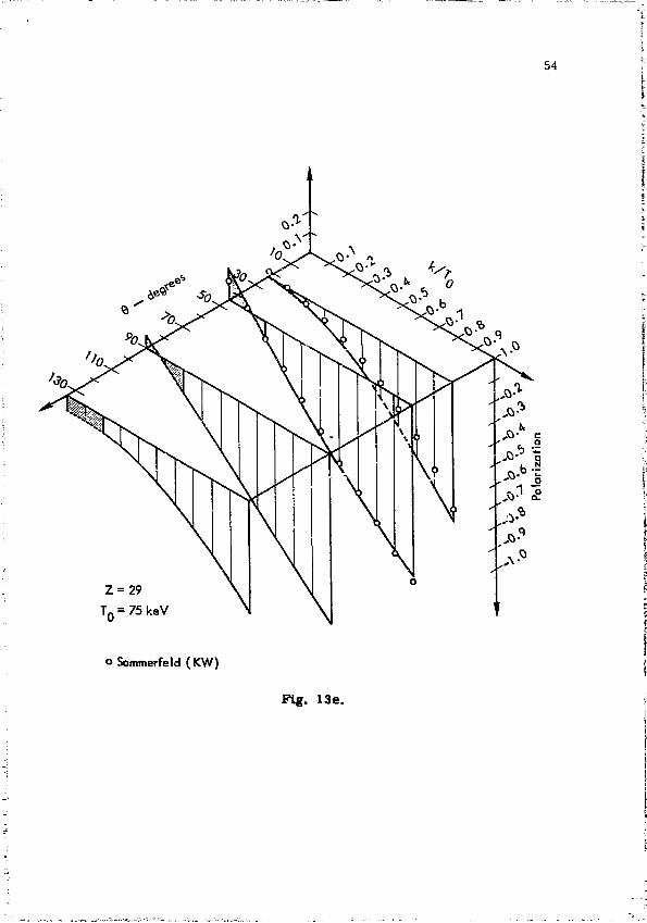
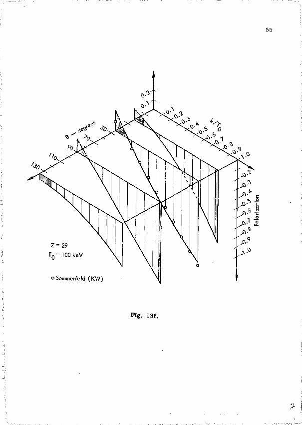
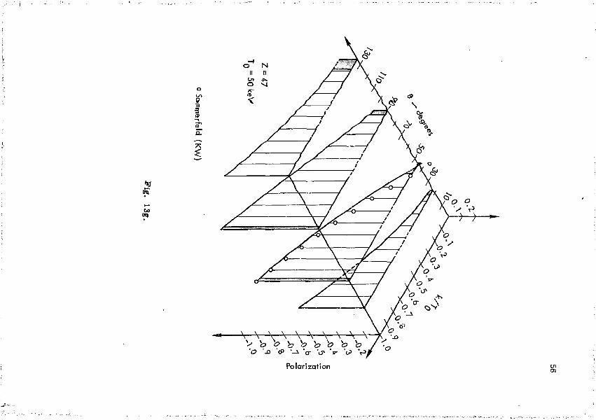
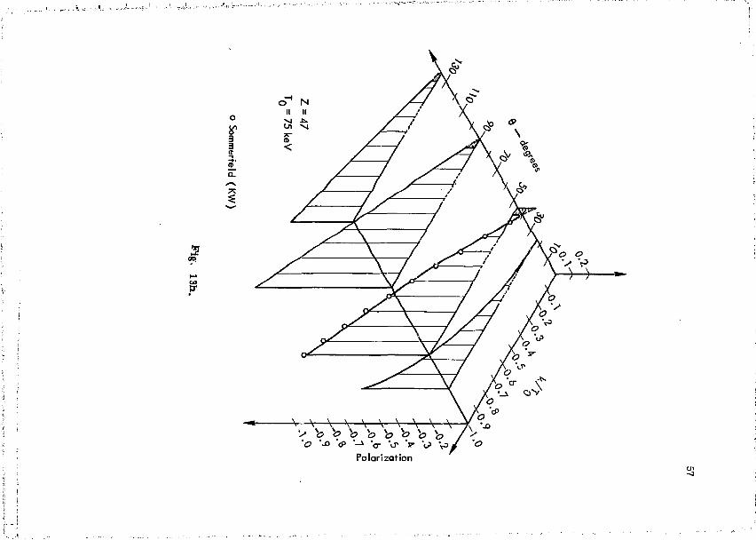
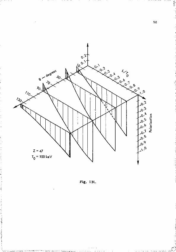
Experimental results for the 48 cases measured a r e presented in Fig. 13a-l. Polarization is plotted as a function of both photon energy (k/T0, photon energy relative to the incident electron energy), and emission angle 9. Positive values indicate polarization perpendicular to the bremsstrahlung reaction plane, and negative values polarization parallel to the reaction plane. Shaded regions at the high- or low-energy ends of some plots indicate extrapolations of the data. Dashed segments of the grid lines indicate regions of the spectra where charac­teristic x-ray lines of the target appeared and polarization results were interpolated. Also, for cases in which reasonable agreement with theory was obtained, calculated points a re indicated on the plots.

o Sommerfeld (KW)

• Tseng and Pratt

Fig. 13a. Linear polarization plotted as a function of both photon energy k / T 0 , and emission angle 6. Photon energy is expressed relative to the incident electron energy, To. Positive (negative) values indicate perpendicular (parallel) polarization, f.haded regions indicate extrapolations of the polarization data, and dashed-line segments indicate interpolation of same.

51

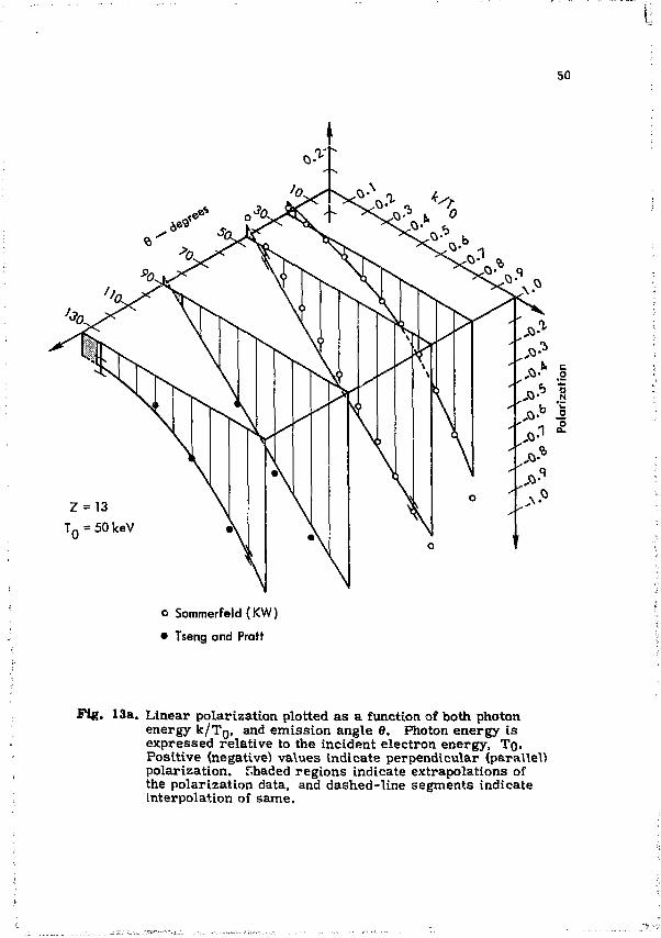
T Q = 75 keV

o Sommerfeid(KW)

• Tseng and Pratt

o a.

Fig. 13b.

52

'*>

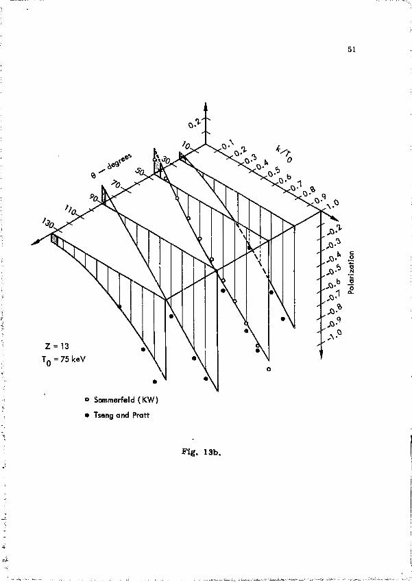
Z = 13 T Q = 100keV

Tseng and Pratt

Fig. 13c.

53

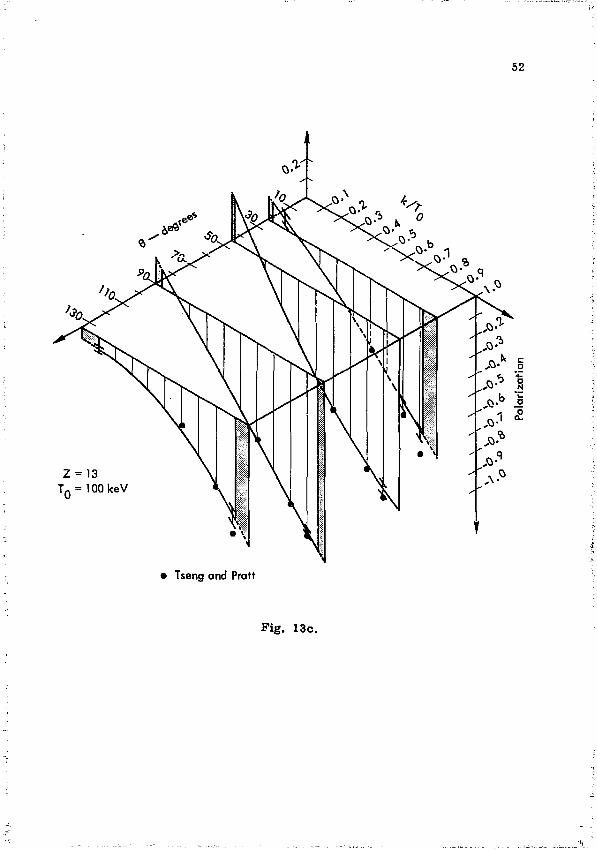
Z=29

TQ = 50 keV

oSommerfeld (KW)

&-1 •?> i.

0-

Fig. 13d.

54

,&<$* s0

TQ = 75 keV

oSommerfeld (KW)

Pig. 13e.

55

' *

Z = 29 T Q = 100 keV

oSommerfeld (KW)

Pig. 13f.

? l

to

1

V b b b fe b b b b / < '(? -O tf> '-A "a- \j» V V V 3 /

Polarization

5? OB

Polarization

53

Fig. 131,

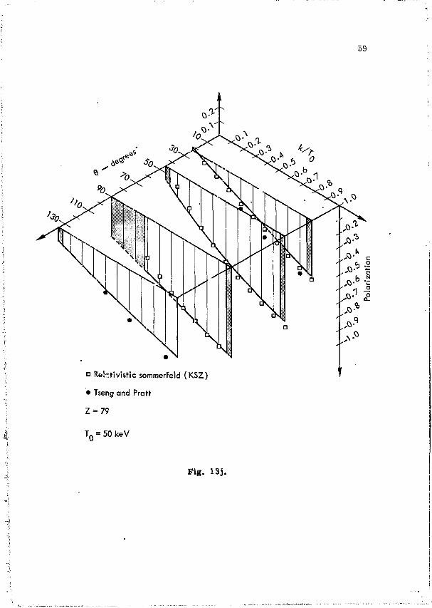
59

o Relstivistic sommerfeld (KSZ)

• Tseng and Pratt

Z = 79

TQ = 50 keV

Fig. I 3 j .

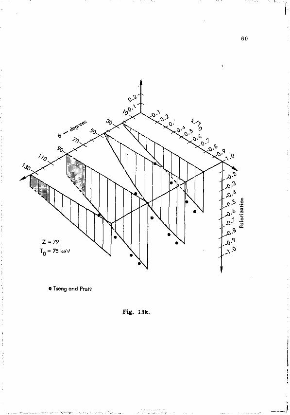
60

T Q = 75 keV

• Tseng and Pratt

Fig. 13k.

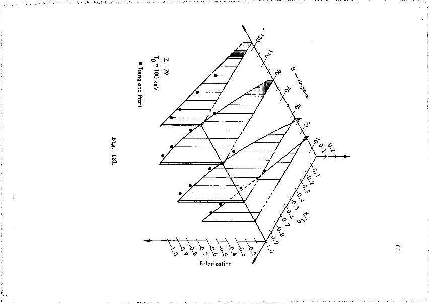
*1 TO

Polarization

62

Polynomials oi degree 1 through 4 were fit to the data using the least-square technique. A measure of the goodness of the fit was evaluated by determining the value of X square divided by the number of degrees of freedom. With very few exceptions, the fit was well

2 determined. Over 50% of the cases had X /f values between 0.8 and 1.2, and 70% had values between 0.7 and 1.3. The number of degrees of freedom was typically 400. The duUa in Fig. 13 are plots of the best polynomial fits obtained in each case. Table 3 lists the degrees and coefficients of these polynomials.

A. k-Dependence of Polarization

The qualitative dependence of linear polarization upon photon energy was predicted in Section II by considerirg a classical descrip­tion of bremsstrahlung. High-energy photons tend to be polarized parallel to the reaction plane, and low-energy photons perpendicular to this plane. This dependence was observed in all 48 cases presented in Fig. 13.

B. 2-Dependence of Polarization

In the bremsstrahlung process, the Coulomb field of the nucleus may alter the direction of the incident electron before the photon is emitted. Referred to as the Coulomb effect,^ this results in a decrease in the observed polarization. The magnitude of this effect increases with Z and predicts an inverse Z-dependence of polarization.

The experimental data substantiate this Z-dependence for both parallel and perpendicular polarization. This is illustrated in Figs. 14a through 14d which show polarization as a function of both k /T Q and Z. These curves include four combinations of 8(45° and 90°) and TQ(50 keV and 100 keV). They clearly illustrate the trend for all energies and angles. The low-energy end of the spectrum is seen to exhibit its most dramatic dependence upon Z at angles for which the polarization is a maximum, i.e., 0 a 45° for T n = 100 keV and

In general, the Coulomb effect refers to the difference between the exact and the Born Approximation bremsstrahlung cross section (see Refs. 4 and 18.

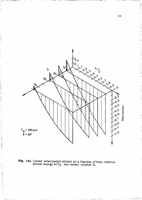
63

T Q = 100keV 9=45°

o Q.

Fig. 14a. Linear polarization plotted as a function of both relative photon energy k / T 0 , and atomic number Z.

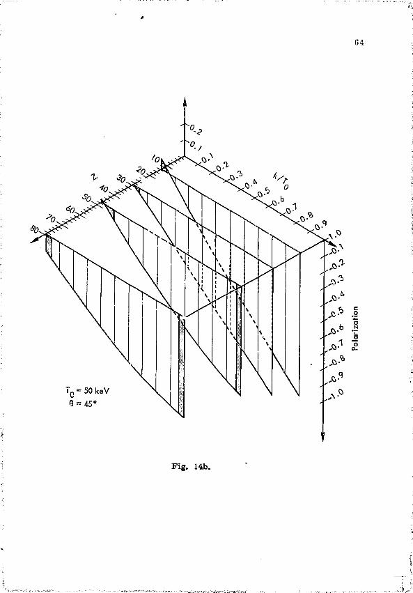
T 0 = 50 keV 9 = 45°

Fig. 14b.

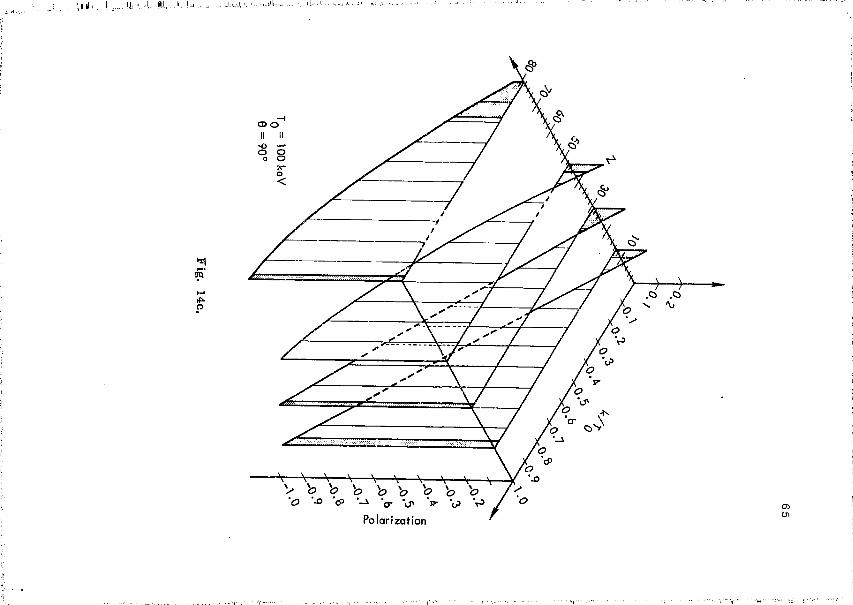
iill.,,....! L.... U, U - . •> h.-!:J

TO

if-O

CD O II II

•o o 0

100

n> <

"S 5 1 Y

V b b b & & o b> & -D '(P -_i -Q. - j , V 'tP V

Polarization en en

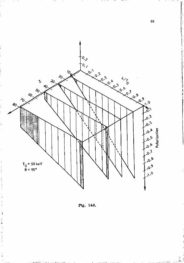
66

T Q = 50 keV 9 = 90°

Fig, 14d.

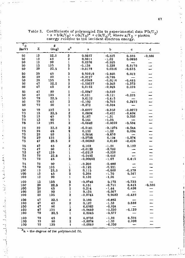
67

Table 3. Coefficients of polynomial fits to experimental d = a +b(k/T 0 ) + c ( k / T 0 r + c(k/T a ) 3 , where K / T 0 = energy relative to the incident electron energy.

data P(k/T ) photon

* 0 e (keV) z (deg) a n a b c d

50 13 22.5 3 0.0657 -0.525 0.595 -0.866 50 13 45 2 0.0611 -1.02 0.0655 . 50 13 90 1 0.0376 -0.995 50 13 135 2 -0.138 0.238 0.8175 50 29 22.5 2 -0.0178 0.0316 -0 .635 — 50 29 45 2 0 t 0 0 9 i 9 -0.805 0.012 50 29 90 1 -0.0127 -0.795 50 29 135 2 -0.0948 -0.0116 -0 .465 — 50 47 22.5 2 -0.C0337 -0.202 -0.273 — 50 47 45 2 0.0192 -0.945 0.239 — 50 47 90 1 -0.0947 -0.630 50 47 135 2 -0.121 -0.111 -0 .233 — 50 79 22.5 1 0.0122 -0.415 — — 50 79 45 2 -0.102 -0.765 0.2473 — 50 79 90 1 -0.272 -0.384 — — 50 79 135 2 -0.0977 -0.358 -0 .0273 75 13 22.5 2 0.0604 -0,421 -0.404 — 75 13 45 2 0.167 -1,31 0.253 — 75 13 90 1 0.141 -1.05 — — 75 13 135 2 -0.0648 -0,0029 -0.534 — 75 29 22.5 2 -0.0141 -0.1275 -0.544 — 75 29 45 2 0.153 -1.22 0.254 — 75 29 90 1 0.0654 -0.870 — — 75 29 135 2 -0.0799 0.124 -0.574 — 75 47 22.5 2 -0.00343 0.0140 -0.434 — 75 47 45 2 0.102 -1.01 0.199 75 47 90 1 -0.0123 -0.780 — — 75 47 135 1 -0.0219 -0.338 — 75 79 22.5 1 -0.0102 -0.416 — — 75 79 45 2 -0.00692 -1.07 0.419 — 75 79 90 • -0.209 -0.488 — 75 79 135 1 -0 .122 -0.221 — —

100 13 22.5 2 0.115 -0.689 -0.170 — 100 13 45 2 0.266 -1.70 0.547 — 100 13 90 1 0.136 -1.06 — — 100 13 135 2 -0.0746 0.178 -0 .732 100 29 22.5 3 0.151 -0.711 0.413 -0.595 100 29 45 2 0.214 -1.44 0.408 — 100 29 90 1 0.135 -0.967 — — 100 29 135 2 -0.0743 0.0682 -0 .439 — 100 47 22.5 1 0.100 -0.693 — 100 47 45 2 0.187 -1.53 0.628 — 100 47 90 1 0.0983 -0.924 — — 100 47 135 2 -0.0489 -0.230 -0 .139 — 100 79 22.5 1 0.0345 -0.577 — — 100 79 45 2 0.0736 -1.32 0.576 — 100 79 90 2 -0.0274 -1.03 0.398 — 100 79 135 1 -0.0869 -0.330 — —

n = the degree of the polynomial fit.

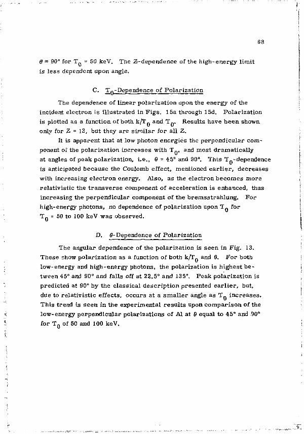
68

6 ~ 90° for T„ = 50 keV. The 2-dependence of the high-energy limit is less dependent upon angle.

C. TQ-Dependence of Polarization

The dependence of linear polarization upon the energy of the incident electron is illustrated in Figs. 15a through 15d. Polarization is plotted as a function of both k/T„ and T„ . Results have been shown only for Z = 13, but they are similar for all Z.

It is apparent that at low photon energies the perpendicular com­ponent ox the polarization increases with T 0 , and most dramatically at angles of peak polarization, i.e„ 0 = 45° and 90°. This T,.-dependence is anticipated because the Coulomb effect, mentioned ear l ier , decreases with increasing electron energy. Also, as the electron becomes more relativistic the t ransverse component of acceleration is enhanced, thus increasing the perpendicular component of the bremsstrahlung. For high-energy photons, no dependence of polarization upon T_ for T„ = 50 to 100 keV was observed.

D. 9-Dependence of Polarization

The angular dependence of the polarization is seen in Fig. 13. These show polarization as a function of both k/T Q and 9. For both low-energy and high-energy photons, the polarization is highest be­tween 45° and 90° and falls off at 22.5° and 135°. Peak polarization is predicted at 90° by the classical description presented ear l ier , but, due to relativistic effects, occurs at a smaller angle as T„ increases. This trend is seen in the experimental resul ts upon comparison of the low-energy perpendicular polarizations of Al at 9 equal to 45° and 90° for T A of 50 and 100 keV.

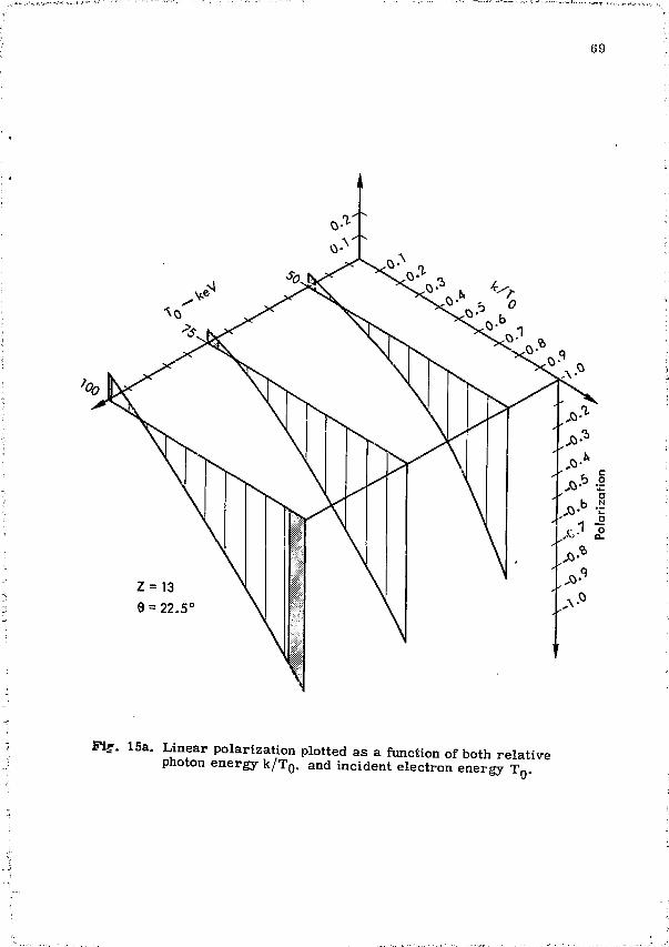
69

L. Linear polarization plotted as a function of both relative photon energy k/Tg, and incident electron energy T„.

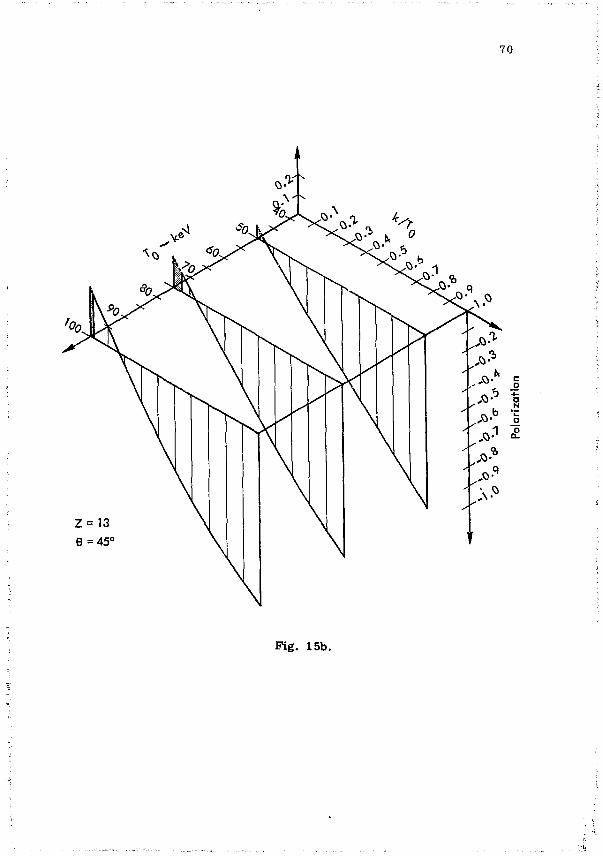
70

Fig. 15b.

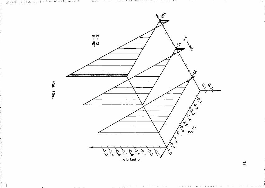
TO

O

O N II 11

> to 'O '-O "rf> * - i "o-

Polarizafion

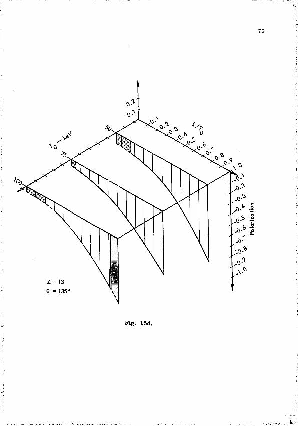
72

X \

> e

" ^ * .

%

Z = 13 e = 135°

*>. ,0-

jo-

J&- -2

„v

O-

Fig. 15d.

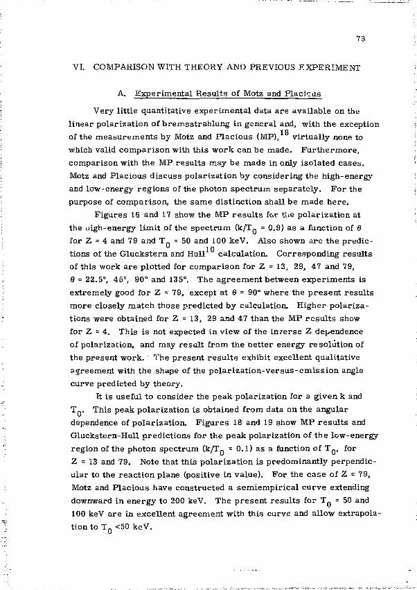
73

VI. COMPARISON WITH THEORY AND PREVIOUS EXPERIMENT

A. Experimental Results of Motz and Placicas

Very little quantitative experimental data are available on the linear polarization of bremsstrahlung in general and, with the exception

18 of the measurements by Motz and Placious (MP), virtually none to which valid comparison with this work can be made. Furthermore, comparison with the MP results may be made in only isolated cases. Motz and Placious discuss polarization by considering ths high-energy and low-energy regions of the photon spectrum separately. For the purpose of comparison, the same distinction shall be made here.

Figures 16 and 17 show the MP resul ts for the polarization at the nigh-energy limit of the spectrum (k/TQ = 0.9) as a function of 8 for Z = 4 and 79 and T n = 50 and 100 keV. Also shown are the predic-

10 tions of the Gluckstern and Hull calculation. Corresponding results of this work are plotted for comparison for Z = 13, 29, 47 and 79, 6 = 22.5", 45°, 90° and 135°. The agreement between experiments is extremely good for Z = 79, except at 8 = 90° where the present results more closely match those predicted by calculation. Higher polariza­tions were obtained for Z = 13, 29 and 47 than the MP resul ts show for Z = 4. This is not expected in view of the inverse Z dependence of polarization, and may result from the better energy resolution of the present work. ' The present resul ts exhibit excellent qualitative agreement with the shape of the polarization-versus-emission angle curve predicted by theory.

It is useful to consider the peak polarization for a given k and T 0 . This peak polarization is obtained from data on the angular dependence of polarization. Figures 18 and 19 show MP resul ts and Gluckstern-Hull predictions for the peak polarization of the low-energy region of the photon spectrum (k/T f l = 0.1) as a function of T„, for Z = 13 and 79. Note that this polarization is predominantly perpendic­ular to the reaction plane (positive in value). For the case of Z = 79, Motz and Placious have constructed a semiempirical curve extending downward in energy to 200 keV. The present results for T Q = 50 and 100 keV are in excellent agreement with this curve and allow extrapola­tion to T n <50 keV.

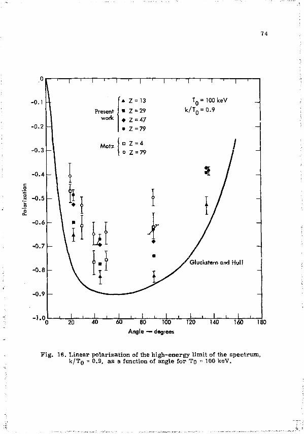
74

-0.7 -

-T 1 r -i 1 r I r " > — r

Present work

Motz

| * Z=13 T 0 =100keV

• Z = 29 k /T Q = 0.9

• Z=47 • Z = 79

• Z = 4 o Z = 79

'• 6

i.

j I i I i _ , J i_ J i L

Gluckstern and Hull

_L J I I l_ "0 20 40 60 80 100 120

Angle — degrees 140 160 180

Fig. 16. Linear polarization of the high-energy limit of the spectrum, k/Tn = 0.9, as a function of angle for TQ =: 100 keV.

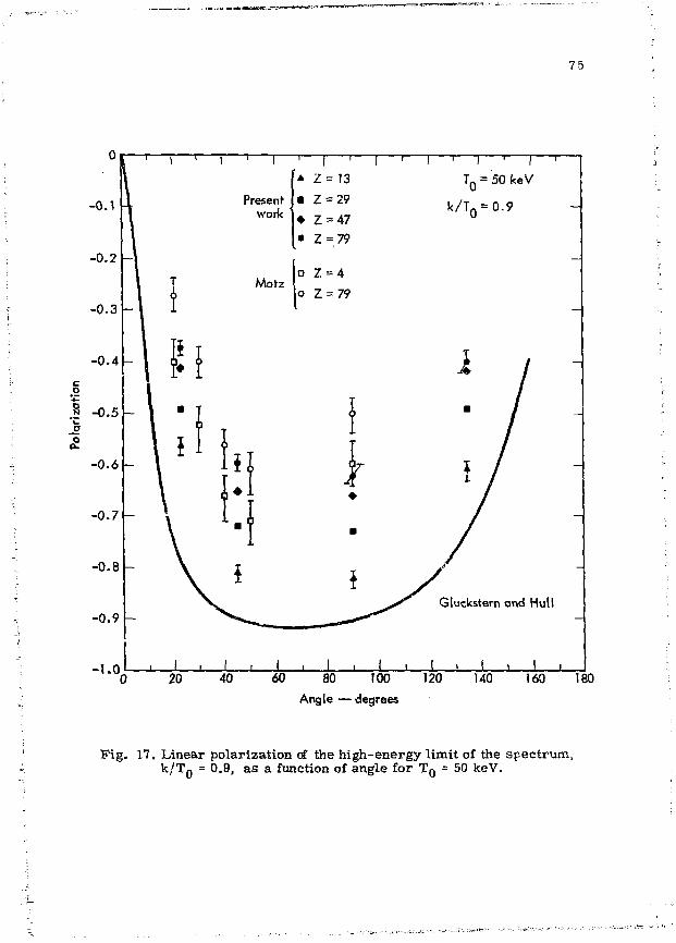
7 5

-i 1 r

* Z = ?3 Present

work • Z = 29 • Z = 4 7 • Z = 79

Morz o Z = 79

-i—i—'—r

TQ = 50 keV

k /T Q = 0.9

I . I -I L L J I L

Gluckstern and Hull

J 1. J -0 20 40 60 80 100 120 140 160 180

Angle — degrees

Fig. 17. Linear polarization of the high-energy limit of the spectrum, k / T Q = 0.9, as a function of angle for T Q = 50 keV.

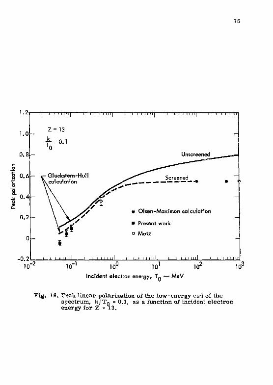
76

' . * i 1—i i i 11 H I 1—i i i i i H I 1—i i i i i H I 1—i i i i m i 1—i i i i i n

1.0

0.8

0.6

0.4

0.2

Z = 13

•£- = 0.1 'o

Unscreened

• ©

• Olsen-Maximon calculation

• Present work

o Motz

-0.21 i—i i i I m l I ' ' ' " " I i i i i m i l i i i i i n i l i i i i i i n 10 -2 10" ' 10 u 10 1 10^

Incident electron energy, T Q — MeV

10

Fig. 18. Peak linear polarization of the low-energy eni of the spectrum, k/Tg = 0.1, as a function of incident electron energy for Z = 13.

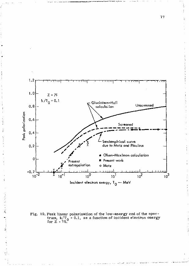
77

1.21 1—i i 11 irn 1—i i T I T i n 1—i i n M M

1.0

0.8

c

1 0.6

o Q .

^ 0.4 o o

0.2

-0.2

-i—i M i nil 1—i I I rrrr

Z = 79

k / T 0 = 0.1

10

Gluckstern-Hul! calculation

''' s U Jif * due to Motz and Placious

S r*^ *— Semiempiricai curve

_1 •' ' A - " ' •

• Olsen-Maximon calculation

/ Present B Present work 1* extrapolation o Motz

i lJ 1 I I I I 1 I I I I i i i ' i i l l _l I M i l l -1

-I I I - t-,1 10 ' 10" 10' 10 '

Incident electron energy, T n — MeV

10"

Fig. 19. Peak linear polarization of the low-energy end of the spec­trum, k / T n =0 .1 , as a function of incident electron energy for Z = 79.

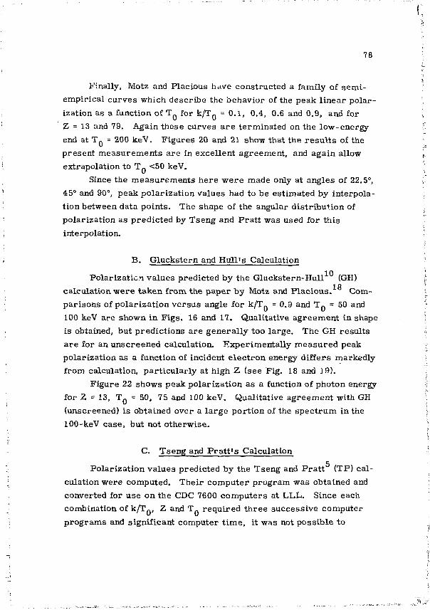
78

Finally, Motz and Placious have constructed a family of semi-empirical curves which describe the behavior of the peak linear polar­ization as a function of T for k /T Q = 0.1, 0.4, 0.6 and 0.9, and for Z = 13 and 79. Again these curves are terminated on the low-energy end at T Q = 200 keV. Figures 20 and 21 show that the resul ts of the present measurements are in excellent agreement, and again allow extrapolation to T 0 <50 keV.

Since the measurements here were made only at angles of 22.5°, 45° and 90°, peak polarization values had to be estimated by interpola­tion between data points. The shape of the angular distribution of polarization as predicted by Tseng and Prat t was used for this interpolation.

B. Gluckstern and Hull 's Calculation

Polarization values predicted by the Gluckstern-Hull (GH) 1 O

calculation were taken from the paper by Motz and Placious. Com­parisons of polarization versus angle for k /T 0 = 0.9 and T Q = 50 and 100 keV are shown in Figs. 16 and 17. Qualitative agreement in shape is obtained, but predictions are generally too large. The GH results are for an unscreened calculation. Experimentally measured peak polarization as a function of incident electron energy differs markedly from calculation, particularly at high Z (see Fig. 18 and 19).

Figure 22 shows peak polarization as a function of photon energy for Z = 13, T Q = 50, 75 and 100 keV. Qualitative agreement with GH (unscreened) is obtained over a large portion of the spectrum in the 100-keV case, but not otherwise.

C. Tseng and P ra t t ' s Calculation

Polarization values predicted by the Tseng and Prat t (TP) cal­culation were computed. Their computer program was obtained and converted for use on the CDC 7600 computers at LLL. Since each combination of k/T f l , Z and T n required three successive computer programs and significant computer t ime, it was not possible to

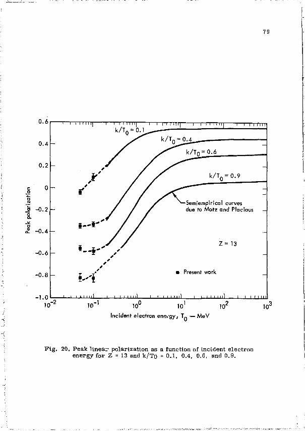
f

79

0.6

0.4

0.2 -

0 -

I -" o

£. - 0 . 4 -

-0.6 -

-0.8 -

-1.0 10

r i i i i i i i| i 1 1 1 1

k / T n

ii[ - r = 0 - 1 -

1 1 1 I Mi[ 1 1 1 I I 1 111 1 —l—TT I I I ! r i i i i i i i| i 1 1 1 1

k / T n

ii[ - r = 0 - 1 -

k / T Q = k / T Q = —

_ *

k /Tn = 0 . 6

_ *

-

k / T Q = 0 . 9

-- -

— — Semiempirical curves

due to Motz and Placious

i - i ' y

i

i .-S-- y

1 1 1 1 1 111 L

* *

- i I.J i n i l i

•

Z = 13

Present work

1 1 1 1 1 1 1 1 ) 1 T 1 J-LU -2 10 - 1 10° 101 102

Incident electron energy, T- — MeV 10°

Fig. 20. Peak l inear polarization as a function of incident electron energy for Z = 13 and k/To = 0.1, 0.4, 0.6, and 0.9.

80

0.5

0.3 -

10 ' 10 10' 10"

Incident electron energy T- — MeV

Fig. 21. Peak linear polarization as a function of incident electron energy for Z = 79 and k / T Q = 0.1, 0.4, 0.6, and 0.9.

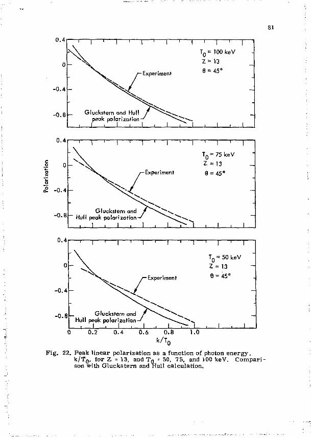
0.4

- 0 . 4 -

-0.8

1 1 •

- ^v 1 ' 1 ' 1 ' 1 1 1 '

T Q = 100 keV Z = 1 3

-

i— Experiment 9 = 45°

\ ^

_ Gluckst ern and Hull f ^""•~^>»

-

peak _. 1 1 L

po la r i za t ion - ' ^"^•^"~--1 i 1 i 1 i 1 , 1 ,

0.4

c o

-0.4

-0.8 Gluckstern and

Hull peak polarization _ i 1

TQ = 75 keV Z = J3 9 = 45°

0.4

0 -

- 0 . 4 -

- 0 . 8 -

1 ' 1 ' 1 ' 1 ' 1 1 1 ' 1

TQ = 50 keV -

" ^ N ̂ /—Experiment

Z = 13 9 = 45°

^ /

Gl Hull peak

. 1 polar izat ion- ' -s-^_ " " ^

1 , 1 , 1 7»- 1 , 1 i 1

-

0.2 0.4 0.6 0.8 k / T n

1.0

Fig. 22. Peak linear polarization as a function of photon energy, k / T 0 , for Z = 13, and TQ = 50, 75, and 100 keV. Compari­son with Gluckatern and Hull calculation.

82

c o n s i d e r every combina t ion m e a s u r e d . Cons squerrtly, the following r e p r e s e n t a t i v e ca se s w e r e s e lec ted:

T Q (keV) Z k / T Q

50 13 0 .4 ,0 .6 ,0 .8 50 79 0 .4 ,0 .6 ,0 .9 75 13 0 .6 ,0 .8 ,0 .9 75 79 0 . 4 , 0 . 6 , 0 . 8 , 0 . 9

100 13 0 .6 ,0 .8 ,0 .9 100 79 0 . 4 , 0 . 6 , 0 . 8 , 0 . 9

F i g u r e s 23a through 23f show both T P and p r e s e n t e x p e r i m e n t a l r e s u l t s for po la r i za t ion v e r s u s angle. Also, T P r e s u l t s a r e indicated on F i g s . 13a, b , c, j , k, 1.

F o r T n = 100 keV and Z = 13, a g r e e m e n t is excel lent ; and for T Q = 100 keV and Z = 79, it is r e a sonab l e . However , for l ower e l e c ­t r o n ene rg i e s , T . = 75 and 50 keV, the ca lcu la ted va lues qual i ta t ive ly a g r e e in shape but a r e cons is ten t ly h igher t han exper iment .

D. Haug ' s Ca lcu la t ion

Haug has ca lcu la ted the po l a r i z a t i on at the h igh-energy l i m i t of the s p e c t r u m for T Q = 100 keV and Z = 4 and 79. F i g u r e 24 c o m ­p a r e s his r e su l t s with exper imen t , and shows r ea sonab le a g r e e m e n t at a l l angles for Z = 79. At lower Z, the e x p e r i m e n t a l p o l a r i z a t i o n i s l e s s for d = 22.5° and 135° than in te rpo la t ion be tween Haug ' s r e s u l t s for Z = 4 and 79 would imply . Haug ' s va lues a r e for an u n s c r e e n e d nuc l eus .

E. Sommer fe ld ' s T h e o r y

1. Ki rkpa t r i ck and Wiedmann ' s Calcula t ion

A p r o g r a m was w r i t t e n to compute t h e po la r i za t ion as ca lcu la ted 9

by Ki rkpa t r ick and Wiedmann (KW). A g r e e m e n t with e x p e r i m e n t was g e n e r a l l y poor , as expected , s ince the Sommerfe ld ca lcu la t ion does not include sc reen ing o r r e l a t i v i s t i c effects . However, r e a s o n a b l e a g r e e m e n t was obtained in some c a s e s , but only at forward angles (22.5° o r 45°). Also, a g r e e m e n t genera l ly tended to improve for low

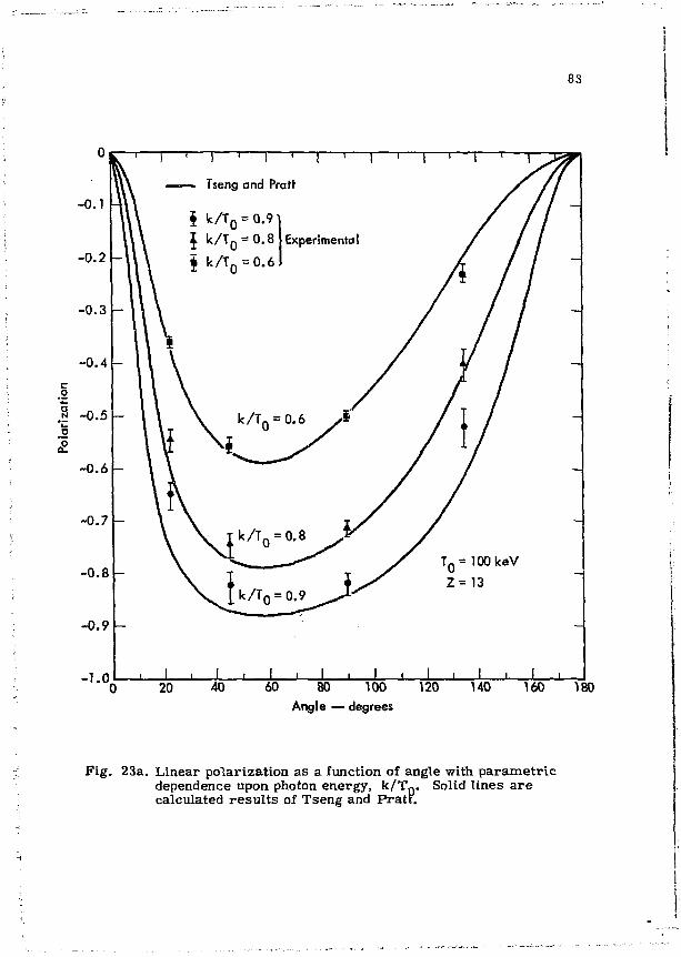
83

-1.0

TQ = 100 keV

i , l . i J >_J i L I • I I I L 20 40 60 80 100 120 140 160 180

Angle — degrees

Fig. 23a. Linear polarization as a function of angle with parametr ic dependence upon photon energy, k/Tg. Solid lines are calculated resul ts of Tseng and Prat t .

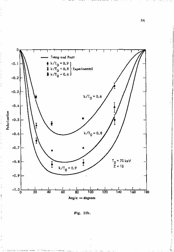
84

- l .O j 1- j l i_ _L I L. J I L 20 40 60 80 100 120 140 160 11

le — degrees

Fig. 23b.

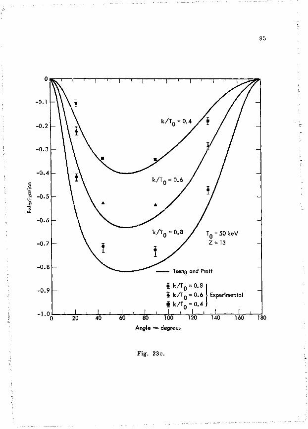
85

-0.1

-0.2 -

-0.3

-0.4 -

I -0.5 o

-0.6 -

-0.7

-0.8

-0.9

•K—T- 1 ' 1 ' 1 ' 1 ' 1 ' 1 ' ' ' i</^

- 1 w k /T Q = 0.4 A / -

\ «

V 1

- w k /T Q = 0.6 /

-\ * A /

\

k/T Q = 0.8 / T Q = 50 keV

- 1 . 0

Z = 13

Tseng and Pratt

Jk/T c

I k/T,

- I I 1 I I I L J i L

0.8 0.6

i kA 0 =0.4j i i i

Experimental

J i L 20 40 60 80 100 120

Angle — degrees

J_ 140 160 180

Fig. 23c.

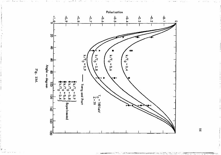
Polarization

o 1

o o 1 o

i O

1 o

1 o 1

o -o 00 VJ oc O l •t* CO S3

* 3 w

5-•

00 o

to 1 GO £-a <8 _ i o o

6

s il

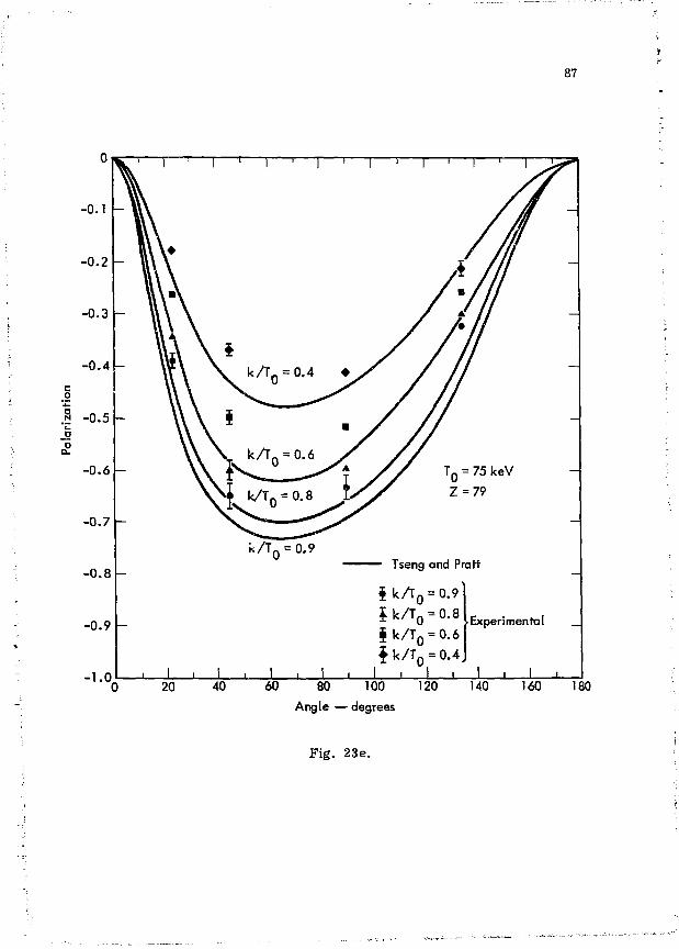
87

-0.8

-0.9

-1.0

k / T 0 = 0.9 Tseng and Pratt

20 40 60 80 100 Angle — degrees

i k A 0 = o.9 | k / T 0 = 0.8 £ k / T 0 = 0.6 $ k / T Q = 0.4.

J I I l _

• Experimental

_1_ 120 140 160 180

Fig. 23e.

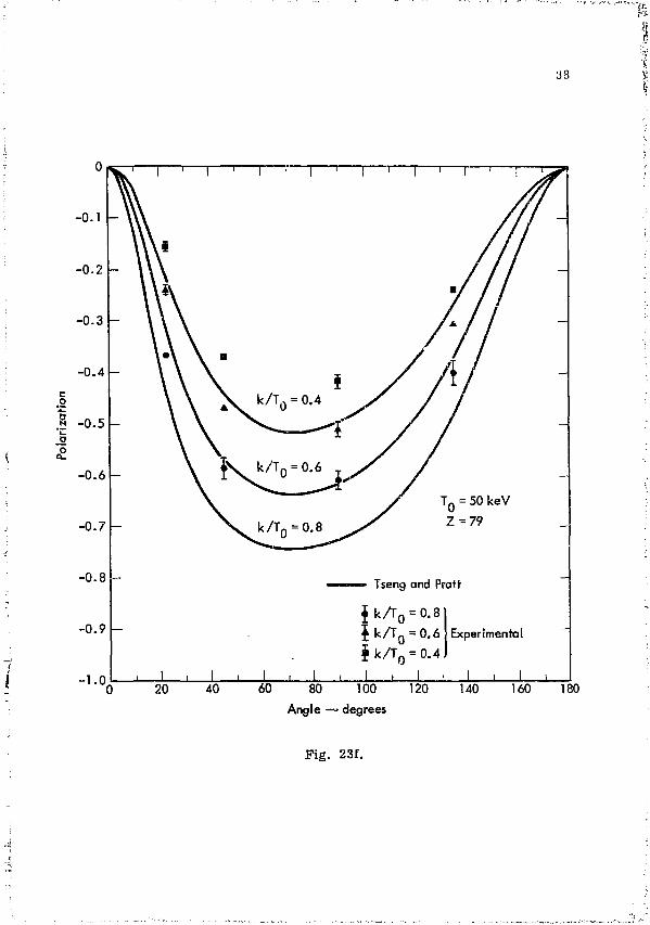
33

-0.8

-0.9

-1.0.

T 0 = 50 keV

Tseng and Pratt

$ k A 0 = 0.8 | k / T Q = 0.6 Jk/T Q = 0.4

Experimental

i i i

20 40 60 80 100 Angle — degrees

J I L 120 140 160 180

Fig. 23f.

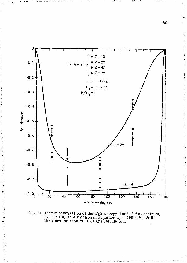
89

20 4 0 60 80 100 120 UQ 160" 180 Angle — degrees

Fig, 24. Linear polarization of the high-energy limit of the spectrum, k / T 0 = 1.0, as a function of angle for TQ = 100 keV. Solid lines are the resul ts of Haug's calculation.

90

T and low Z, again as expected. KW points are indicated only for cases in which resonable agreement was obtained (Figs. 13a, 13b, 13d through 13h).

2. Kulenkampff, Scheer and Zeit ler 's Relativistic Transformation

The computer program which calculated KW bremsstrahlung 14

polarization also applied the Kulenkampff et al. relativistic t r ans ­formation to the resul ts . This t ra ." formation is valid only for elec­tron energies <40 keV, and should not apply to the energies employed here. However, for forward angles and Z = 79, agreement was ob­tained for T„ = 50, 75 and 100 keV. These cases are indicated in Fig. 13 j .

VII. CONCLUSIONS

The purpose of this work was to conduct a systematic experi­mental investigation of the linear polarization of low-energy electron bremsstrahlung. Linear polarization was measured as a function of photon energy over a wide range of emission angles and target Z. The results allow interpolation of polarization for all values of 0, Z, and T Q (50 keV < T Q < 100 keV). Quantitative com­parison of present data with previous experimental results, where possible, has produced good agreement.

The observed polarization dependence upon the variables k, T n , 6 and Z is in qualitative agreement with the predictions of theory. Quantitative comparison with the results of individual theories illustrates that some calculations are more successful at predicting polarization than others. A summary of these comparisons follows.

1. The quality of agreement varies from fair to excellent. No pattern is obvious, but trends in the comparisons may be seen in Fig. 25. Only cases of good agreement have been indicated on this figure. In all other cases, agreement was poor.

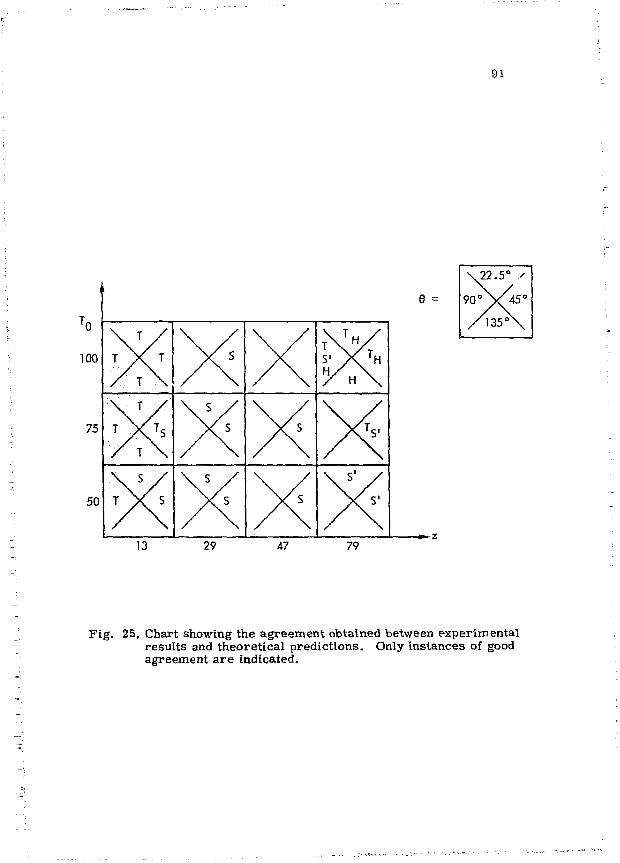
91

'0

100

75

50

e =

22.5° .'

90 ° \ ( 4 5 0

nas'X

13 29 47 79

Fig. 25. Chart showing the agreement obtained between experimental results and theoretical predictions. Only instances of good agreement a re indicated.

92

2. The numerical calculation of Tseng and Pratt is more suc­cessful than other calculations at predicting polarization, particularly for low Z. It should be emphasized that T P calculations were carried out only for Z = 13 and 79 (shaded regions on Fig. 25).

3. The Born approximation calculations (such as Gluckstern and Hull or Fronsdal and Uberall) generally predict polar i ­zation values la rger than observed. However, the GH cal­culation of peak polarization (including screening) shows fair agreement with experiment for low Z.

4. Sommerfeld predictions, whether relativistically transformed or not, cannot generally be applied to this electron energy region. The few instances of agreement obtained may be fortuitous.

Suggestions for Future Work

During the course of this work it has become apparent that several related experiments would be useful for testing the theory more completely. These a r t :

1. Measurement of polarization emphasizing the low k/T Q region of the spectrum.

Observed bremsstrahlung intensities fall off at the low-energy end of the spectrum. Also, polarimeter efficiency is decreased severely for low photon energy. Consequently, experimental resul ts are less certain and more difficult to obtain. Polarization in this region, however, is most sensitive to the screening of the nucleus by orbital electrons, and its determination should be helpful in guiding the calculational treatment of screening.

2. Measurement of polarization for T_ < 50 keV. Little quantitative bremsstrahlung polarization data for very

low electron energy (T Q < 50 keV) exists. However, both the Sommerfeld theory and Tseng and Pratt calculations apply in this region. The difficulty in performing an experiment at these energies is primarily one of obtaining thin targets. An obvious approach would be to attempt the measurement using gas targets and a high-resolution Si(Li) detector.

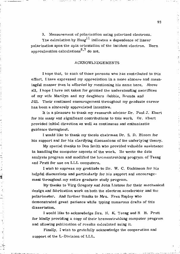
93

3. Measurement of polarization using polarized electrons. The calculation by Haug indicates a dependence of l inear

polarization upon the spin orientation of the incident electron. Born fi 7 approximation calculations ' do not.

ACKNOWLEDGEMENTS

I hope that, to each of those persons who has contributed to this effort, I have expressed my appreciation in a more sincere and mean­ingful manner than is afforded by mentioning his name here. Above all, I hope I have not taken for granted the understanding sacrifices of my wife Marilyn and my daughters Debbie, Brenda and Ji l l . Their continued encouragement throughout my graduate career has been a sincerely appreciated incentive.

It is a pleasure to thank my research advisor Dr. Paul J. Ebert for his many and significant contributions to this work. Dr. Ebert provided initial direction as well as continuous and enthusiastic guidance throughout.

I would like to thank my thesis chairman Dr. S. D. Bloom for his support and for his clarifying discussions of the underlying theory.

My special thanks to Don Smith who provided valuable assistance In handling the computer aspects of the work. He wrote the data analysis program and modified the bremsstrahlung program of Tseng and Pratt for use on LLL computers.

I wish to express my gratitude to Dr. W. C. Dickinson for his helpful discussions and particularly for his support and encourage­ment throughout my entire graduate study program.

My thanks to Virg Gregory and John Lietzke for their mechanical design and fabrication work on both the electron accelerator and the polarimeter. And further thanks to Mrs. Fran Rupley who demonstrated great patience while typing numerous drafts of this dissertation.

I would like to acknowledge Drs. H. K. Tseng and R H. Pratt for kindly providing a copy of their bremsstrahlung computer program and allowing publication of results calculated using it.

Finally, I wish to gratefully acknowledge the cooperation and

support of the L-Division of LLL.

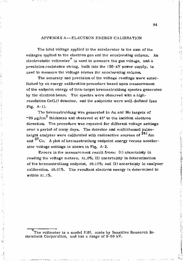
94

APPENDIX A—ELECTRON ENERGY CALIBRATION

The total voltage applied to the accelerator is the sum of the voltages applied to the electron gun and the accelerating column. An electrostatic voltmeter^ is used to measure the gun voltage, and a precision resistance string, built into the 150-kV power supply, is used to measure the voltage across the accelerating column.

The accuracy and precision of the voltage readings were estab­lished by an energy calibration procedure based upon measurement cf the endpoint energy of thin-target bremsstrahlung spectra generated by the electron beam. The spectra were observed with a high-resolution Ge(Li) detector, and the endpoints were well-defined (see Pig. A-l) .

The bremsstrahlung was generated in Au and Mo targets of ~20 /ng/cm thickness and observed at 45° to the incident electron direction. The procedure was repeated for different voltage settings over a period of many days. The detector and multichannel pulse-

241 height analyzer were calibrated with radioactive sources of Am 57

and Co. A plot of bremsstrahlung endpoint energy versus acceler­ator voltage settings is shown in Fig. A-2.

Er rors in the measurement result from: (1) uncertainty in reading the voltage meters , ±1.0%; (2) uncertainty in determination of the bremsstrahlung endpoint, ±0.15%; and (3) uncertainty in analyzer calibration, ±0.01%. The resultant electron energy is determined to within ±1.1%.

The voltmeter is a model ESH, made by Sensitive Research In­strument Corporation, and has a range of 0-60 kV.

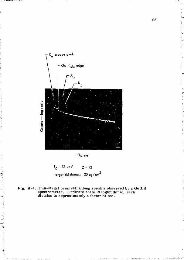
95

K escape peak

Chann

TQ = 75 keV Z = 42

Target thickness : 20 fig/cm 2

Pig. A - 1 . Thin-target bremsstrahlung spectra observed by a Ge(Li) spectrometer. Ordinate scale is logarithmic, each division is approximately a factor of ten.

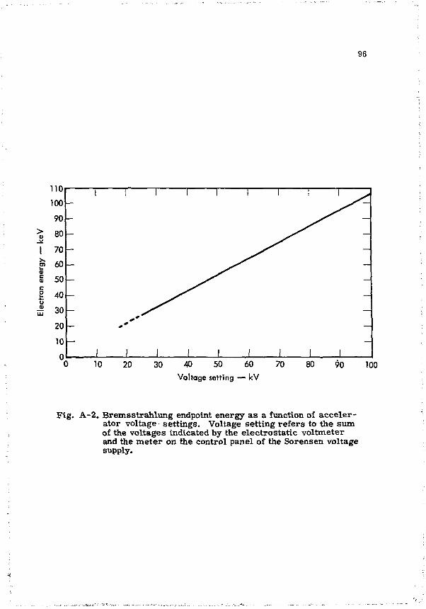
96

10 20 30 40 50 60 70 Voltage setting — kV

80 90 100

Fig. A-2. Bremsstrahlung endpoint energy as a function of acce ler ­ator voltage settings. Voltage setting refers to the sum of the voltages indicated by the electrostatic voltmeter and the meter on the control panel of the Sorensen voltage supply.

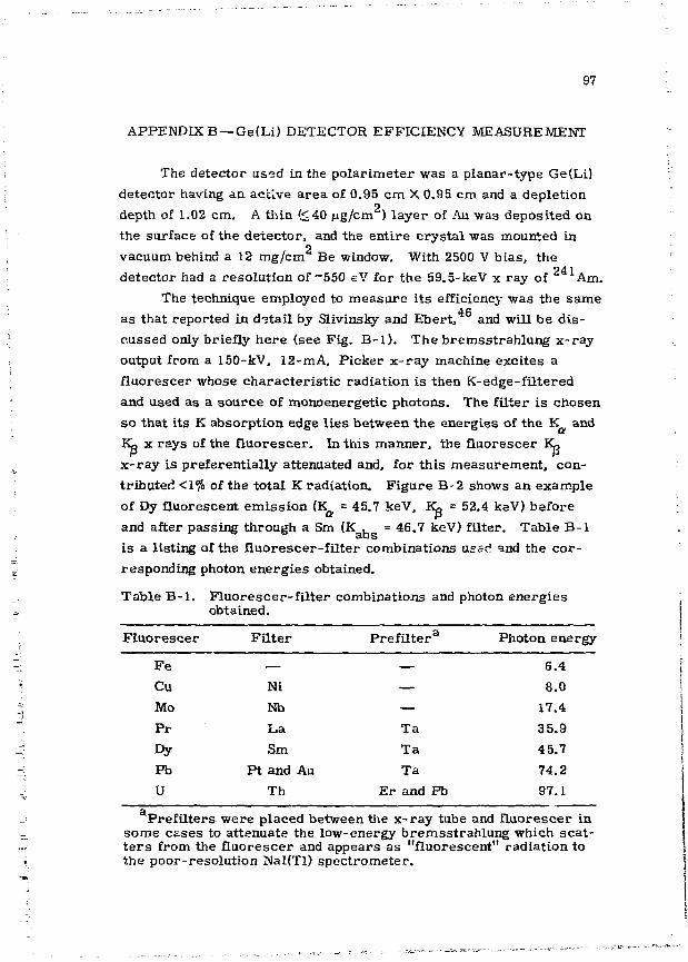
97

APPENDIX B - G e ( L i ) DETECTOR EFFICIENCY MEASUREMENT

The detector usod in the polarimeter was a planar-type Ge(Li) detector having an active area of 0.95 cm X 0.95 cm and a depletion depth of 1.02 cm. A thin (<40 fig/cm ) layer of Au was deposited on the surface of the detector, and the entire crystal was mounted in

2 vacuum behind a 12 mg/cm Be window. With 2500 V bias, the

241 detector had a resolution of ~550 eV for the 59.5-keV x ray of Am. The technique employed to measure its efficiency was the same

as that reported in detail by Slivinsky and Ebert, and will be dis­cussed only briefly here (see Fig. B- l ) . Thebremsstrahlung x-ray output from a 150~kV, 12-mA, Picker x- ray machine excites a fluorescer whose characterist ic radiation is then K- edge -filtered and used as a source of monoenergetic photons. The filter is chosen so that its K absorption edge lies between the energies of the K and Kj x rays of the fluorescer. In this manner, the fluorescer K, x- ray is preferentially attenuated and, for this measurement, con­tributed <1% of the total K radiation. Figure B-2 shows an example of Dy fluorescent emission (K = 45.7 keV, K, = 52.4 keV) before and after passing through a Sm (K , = 46.7 keV) filter. Table B- l is a listing of the fiuorescer-filter combinations used and the cor­responding photon energies obtained.

Table B - l . Fluorescer-f i l ter combinations and photon energies obtained.

Fluorescer Fil ter P re f i l t e r 3 Photon energy

F e — — 6.4 Cu Ni — 8.0 Mo Nb — 17.4 P r L a T a 35.9 Dy Sm T a 45.7 Pb Pt and Au T a 74.2 U Th Er and Pb 97.1

p Prefil ters were placed between the x- ray tube and fluorescer in

some cases to attenuate the low-energy bremsstrahlung which scat­t e r s from the fluorescer and appears as "fluorescent" radiation to the poor-resolution Nal(Tl) spectrometer.

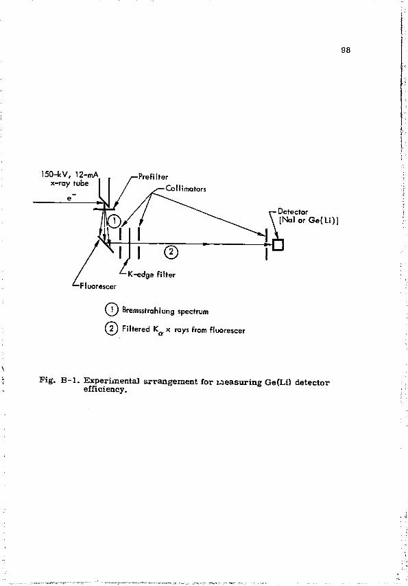
98

150-kV, 12-mA. x-ray rube

-Prefilter -Coll itnators

'-Fluorescer

\V) Bremsstrahlung spectrum

{2J Filtered K f f x rays From fl

Detector [ N a l o r G e ( L i ) ]

uorescer

Fig. B - 1 . Experimental arrangement for measuring Ge(Li) detector efficiency.

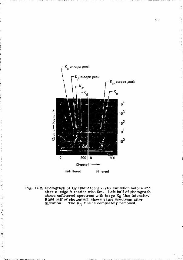
K escape peak

•Kn escape peak K escape peak

500

Channel — » -

Unfilfered Filtered

Fig. B-2. Photograph of Dy fluorescent x- ray emission before and after K-edge filtration with Sm. Left half of photograph shows unfiitered spectrum with large K̂ j line intensity. Right half of photograph shows same spectrum after filtration. The Kg line is completely removed.

100

The absolute in t ens i t i e s of the x r a y s w e r e measu red us ing a to ta l ly absorbing Nal(Tl) s p e c t r o m e t e r (4 m m th i ck X 2.5 cm d iam for hv <, 45.7 keV, and 2.5 c m th ick X 2.5 cm d iam o therwise ) . The Ge(Li) d e t e c t o r was placed in the s a m e loca t ion and g e o m e t r y conf igurat ion a s the Nal(Tl) s p e c t r o m e t e r and i ts efficiency compared to that of the

100% efficient Nal. Eff ic iencies above 100 keV w e r e m e a s u r e d us ing 57 the 122- and 136-keV x r a y s f rom a ca l ib ra t ed IAEA Co s o u r c e .

F i g u r e B-3 shows a plot of the de tec to r efficiency as a function of photon energy. The l o w e r por t ion of the uppe r curve is the pho to -p e a k contr ibut ion to the efficiency while the upper por t ion is the s u m of the counts in the photopeak plus the Ge e s c a p e peak. Also plot ted is the e scape -peak - to -pho topeak ra t io , E P / P P , as a function of photon ene rgy . It can be s e e n tha t the de tec tor is e s s e n t i a l l y b lack (99% ef­ficient) f rom 20 to 70 keV, and the cont r ibu t ion of the escape p e a k

b e c o m e s negligible above 50 keV. These r e s u l t s a r e in exce l len t 46 a g r e e m e n t with those m e a s u r e d by Slivinsky and Eber t .

Since the effect of de t ec to r efficiency c a n c e l s out in a p o l a r i z a ­t i o n m e a s u r e m e n t , the efficiency informat ion, p e r se , is not u sed . However , the e scape -peak - to -pho topeak r a t i o a s a function of ene rgy is applied as a c o r r e c t i o n to the r a w data.

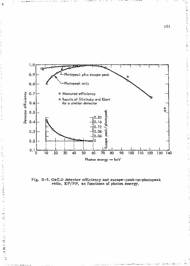
101

^ '— Phofopecik plus escape peak ^ *

1 1 1 1 1

- / ^—Photopeak only -

— o Measured eff ic iency v —

— ^ Results of Slivinsky and Ebert

for a similar detector —

- a - i 0 . 2 0 g"

o

- \ 0.16 _° 0.12 •£ 0.08 "f

1 l**°"-+—n_|__ 0.04 °-0 8. o o

I " 1 1 1 1 , I " i i i i

0.04 °-0 8. o o

I " 1 1 1 1 , I " 10 20 30 40 50 60 70 90 100 110 120 130 140

Photon energy — keV

Fig. B-3 . Ge(Li) detector efficiency and escape-peak-to-photopeak ratio, E P / P P , as functions of photon energy.

102

APPENDIX C—TARGET THICKNESS MEASUREMENT BY X-RAY FLUORESCENCE TECHNIQUE

A technique was developed for determining the mass thickness (mass per unit area) of a thin target by measuring its K x-ray yield when excited by monoenergetic x rays. The method is accurate to better than ±10% and depends upon knowledge of the K-shell photo­electric cross section and fluorescence yield for the target material.

The source of monoenergetic photons is the same as that de-scribed in Appendix B. The target whose thickness is to be meas­ured is excited by these photons, and the resulting fluorescent emission is observed by a Si(Li) spectrometer. Considering the geometry shown in Fig. C-l, it is seen that the ccunt rate of the Si(Li) spectrometer will be

"0 f- /J J. / t u a t u - —

N Si

where

rpT/cos45° - - p P i t M - £ p x £2S. * A e P ^ J e P ^ e s . p d x (C-l)

0 (•*-—= 1 = the photon flux at the defining collimator, \cm*-sec/

A (cm2) = area of defining collimator,

P Vgm/

P \grnj

total mass attenuation coefficient of the target material for the incident photons of energy hvQ,

2\ mass absorption coefficient for photo-gm, ionization of the K-shell of the target for

A* (cm ] _ p \ g m / "

photons of energy hvQ,

total mass attenuation coefficient of the target material for photons of energy equal to the target K x-ray energy, hv,

A detailed description of this technique for routinely producing monoenergetic photons with energy <100 keV is presented in Ref. 47.

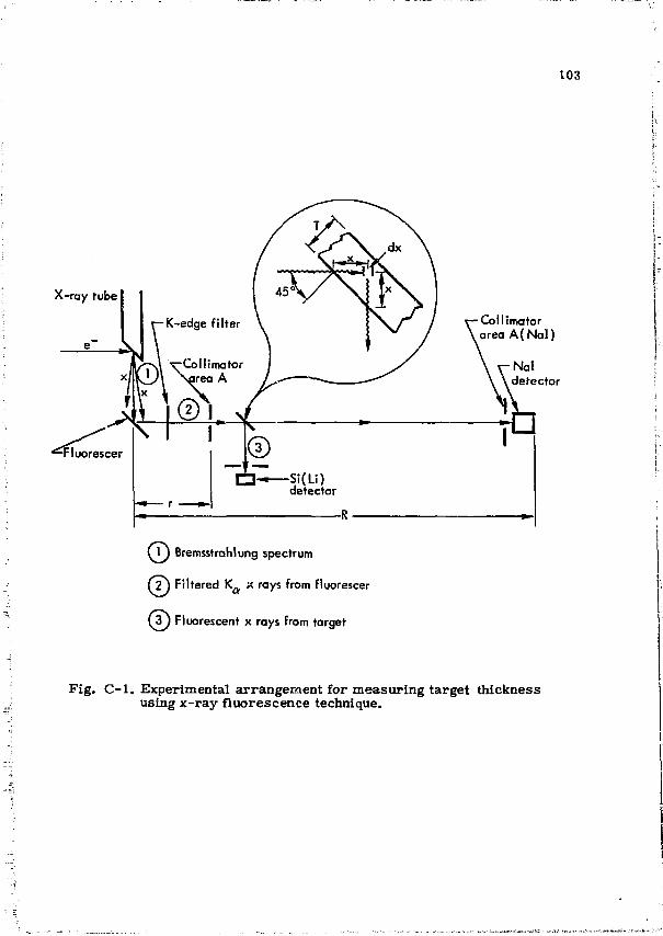
103

X-ray tube

( l ) Bremsstrahlung spectrum

( 2 j Filtered K^ x rays from fluorescer

\2j Fluorescent x rays from target

Col lima tor area A ( N a l )

^ - N a l detector

Fig. C - 1 . Experimental arrangement for measuring target thickness using x-ray fluorescence technique.

104

u = K-sii'sll fluorescence yield of the target material,

I2 g i (ster) = solid angle subtended by the Si(Li) spectrom­eter at the target,

£o: = efficiency of the Si(Li) detector for incident photons of energy hi/ (includes transmission of any material between the target and the detector),

P dx ( ""V) = element of target thickness. \cm /

pT ( 6 x) = total target thickness.

The flux, 4>. incident on the defining collimator is determined by measuring the flux » large distance away from the source with a NaKTl) spectrometer. Relying on the isotropic nature of the source, the flux at the defining collimator is given by:

, R 2 1 ft(Nal) ,_ *"?*Z™™ (C"2)

where

N ( W a I ) ( c ° ^ t s j = count-rate measured by the NaKTl)

A(NaI)(cm ) = area of the Na(Tl) spectrometer. spectrometer, area of the Na

c N a I = e ^ i c i e n ° y °f the Nal(Tl) spectrometer for incident photons of energy hvQ

(includes t ransmission of any material in the beam between the target position and the spectrometer),

R, r (cm) = distances indicated in Pig. C- l . Substituting this expression for ^ into Eq. (C-l) gives

ri _R 2N(NaI) A " e S i n S i * k fPTybos45- - ( ^ y p x NSi -72 3755311-^7-^7- J 6 Pdx. (C-3)

105

Integrating and solving for the target mass thickness, pT, gives

N(Si) pi = mz^L- i n F - In F -cos 45° L N(Nal)

(C-4)

where

A R2 eSi S i f t ) " * " ATNaTT ^2 e N a I I T ' - ^ l U ^

Obviously, for thin targets, Eq. (C-l) can be approximated by

N c . *<£A — — ^ H 4 i - p i £ 5 . (C-6) Si r p cos 45° 47r Si

and Eq. (C-4) by N„. cos 45° 4JT

p T * - £ i , (C-7) y k 0 A - W n s . e S i

where <j> is still given by Eq. (C-2) Uncertainties associated with this technique resuT from un­

certainties in the attenuation coefficients and fluorescence yields used, as well as from spectral impurities in the photon beam/ An erroi of 5% is assigned to each of these three sources with a resulting total uncertainty of approximately ±9%,

— 5 Attenuation coefficients used in this experiment were taken from

McMaster et a l . , 4 8 and fluorescence yields were taken from Fink et al.49 ~ ~

106

APPENDIX D —POLARIMETER ASYMMETRY RATIO, EFFICIENCY AND ENERGY RESPONSE

A computer program has been written to calculate the efficiency, asymmetry ratio, and energy response function of a Compton polarim-eter such as the one described here. The program has been designed to apply generally to the geometry shown in Fig. D- l . It assumes that completely polarized photons enter the polarimeter and are scat­tered from a given volume element of the sca t terer into a given volume element of the detector. It then integrates these scattering events over all volume elements of the scatterer and detector.

Summary of Computer Program

Step 1

The incident photon flux is exponentially attenuated in the scat­te re r to a particular volume element. The total-minus-coherent at­tenuation coefficient of the scat terer material is used for this calcu­lation. Coherent scattering is not considered since this scattering is mainly in the forward direction, and the photon? are assumed to still enter the volume element.

Step 2

The probability of interaction in the sca t terer volume element is computed and then multiplied by the ratio of differential-to-total cross sections to find the photon fraction scattered incoherently and the fraction scattered coherently. The incoherent and the coherent differential cross sections are modified by the appropriate form-factors and scattering functions, respectively.

Step 3

The scattered photon flux is exponentially attenuated in t.h-: scat terer as it exits. The total attenuation coefficient of the scat ter­ing material is used.

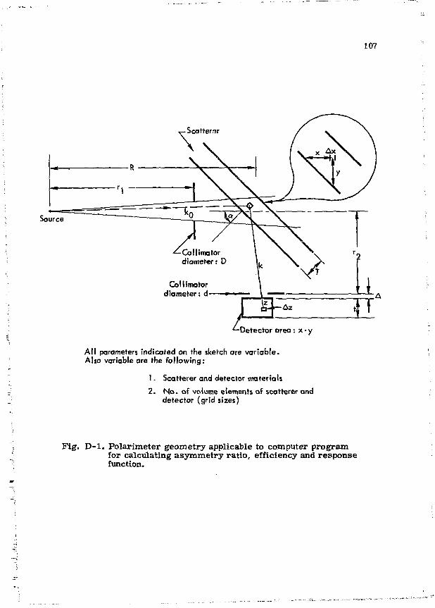
107

-Scatters

Source

Al l parameters indicated on the sketch are variable. Also variable are the following:

1. Scatterer and detector materials

2. N o . of volume elements of scatterer and detector (grid sizes)

Fig. D - 1 . Polarimeter geometry applicable to computer program for calculating asymmetry ratio, efficiency and response function.

108

Step 4

The scattered photon is then exponentially attenuated in the Ge(Li) detector to the given volume element. The total-minus-coherent at­tenuation coefficient for Ge is used.

Step 5

The probability of photon interaction in the volume element of the detector is computed.

Step 6

The program sums over all combinations of scatterer and detec­tor volume elements which are physically possible for a given source and collimator geometry.

Furthermore, the scattered photons are sorted according to energy, and a response function of the polarimeter for a given incident photon energy is obtained. The integral of this response function is the efficiency of the polarimeter and the ratio of efficiencies for 0 = ir/2 and 0 = 0 is the asymmetry ratio.

Mathematical Foundation of the Program

The asymmetry ratio of an ideal Compton polarimeter was de­fined in Section IV-A-4 as

R = doty = ir/2)/dol<t> = 0 ) . (D-l)

For a polari.meter with finite dimensions the asymmetry ratio is defined analogously, i.e.,

R = polarimeter efficiency for 0 = v/2 _ g/2 (D-2) " polarimeter efficiency for 0 = 0 " e 0 "

109

The efficiency of a polarimeter of azimuthal orientation tf for observ­ing a completely polarized photon source of energy k Q and intensity of 1 photon/ster is given by the equation:

£ 4 scat

, >

s det

(1 - t -MA X )

da. — l - S

-iVf -M"Z e e

* f r - V"Az\ r

scat f A "s

det

e V x

X ( l - ( 3 - / iAx, °c „2 e ""y ii g-M z (1 - e - u m A z . (D-3)

where the first double-integral term is the efficiency considering in­coherent scattering only, and the second double-integral term is the efficiency considering coherent scattering only. Obviously, the c o ­herently and incoherently scattered photons wi l l have different energ ies , and the proper attenuation coefficients must be used. The symbol s in the above equation refer to quantities as follows:

An = solid angle subtended by the volume element of the scat terer ;

A n _ = solid angle subtended by the volume element of the detector;

li' = tota l -minus-coherent attenuation coefficient of the sca t t erer material for energy k Q ;

M.ju = total attenuation coefficient of the scat terer m a ­ter ia l for energy k n , k, respect ively;

/i",/£" = tota l -minus-coherent attenuation coefficient of Ge for energy k n , k, respect ive ly;

M ' " . £ = total attenuation coefficient of Ge for energy k Q , k.

respect ive ly , differential (B scattering cros s sect ion (expressed in units of a l inear attenuation coefficient, i .e. , cm ); t factor contains the <fr dependence explicitly;

da. = differential (Klein- Nishima formula) incoherent scattering cros s sect ion (expressed in i l inear attenuation coefficient, i .e. , c m ' ); this

110

dff = differential coherent scattering cross section (ex­pressed ia units of a linear attenuation coefficient, i.e., cm" ); this factor contains the $ dependence explicitly;

S = scattering function for modifying Klein-Nishima cross section to include binding effects of the elec­tron to the atom (values taken from Keating and Vineyard );

2 F = the square of the form-factor for modifying the

differential coherent scattering cross section to account for coherent interference from the orbital electrons of the atom (values taken from Shibata )

x,y,z,Ax,Az = geometrical parameters from Fig. D-l; V t , V . , = volume of the scatterer and detector, respectively. The program computes e *> and e„ by numerically integrating

Eq. (D-3) over all volume elements of the scatterer and area elements of the detector using a CDC 6600 computer. Although the program is designed to integrate over the volume of the Ge(Li) detector, in practice the integration was performed only over the detector area. A polari­zation measurement is independent of detector efficiency, and there­fore the efficiency was not computed. Grid s izes were chosen to

5 3 divide the scatterer into 10 volume elements « 1 mm ) and the de-

2 tector into 225 area elements (~0.44 mm ). The grid size was checked by continually rerunning the program using successively smaller volume and area elements until the effect upon results was negligible.

The program does not account for multiple photon scattering in the scatterer. It is difficult to calculate the error resulting from this but, as stated previously, experimental verification of the calcu­lated polarimeter response to monoenergetic photons allows confidence that errors are small.

Results

Three different polarimeter geometries were used in the present experiment. They differed in scatterer solid angle and thickness, and were characterized by the following parameters (refer to Fig. D-l) .

I l l

A « t

A « t

A « t

Case 1: rx = 9.52 cm R = 13.18 cm D = 1.2; cm a - 45°

r9 = 5.32 cm T = 1.0 cm d = 0.635 cm t = 1 cm

Case 2: r , = 9.52 cm R = 13.18 cm D = 0.635 cm a = 45°

r„ = 5.32 cm T = 1.0 cm d = 0.635 cm t = 1 cm

Case 3 : TJ = 9.52 cm R = 3.18 cm D = 0.635 cm a = 45°

r„ = 5.32 cm T = 0.6 cm d = 0.635 cm t = 1 cm

Response functions, efficiencies, and asymmetry ratios as a function o.f energy were calculated for each of the three cases. Figure D-2 shows a typical calculated response function. The higher-energy peak is the contribution due to coherent scattering, while the lower, m.iin peak is due to incoherent scattering. Figure D-3 shows a plot of efficiency, e, as a function of photon energy, k_, for both the perpendicular ($ = */2) and parallel (̂ = 0) configurations of each case. Figure D-4 shows a plot of the asymmetry ra t io R = (e ;o/e n) versus energy for each case.

The dips in the asymmetry ratios at low photon energies are unexplained, but are of l i t t le consequence because of the very small effect the asymmetry ra t io correction has upon data below 10 keV. The "worst case" uncertainty resulting from this dip is <0.6%. For ease in applying the (R + 1)/(R - 1) correction to the data using the computer program described in Section TV-D, the calculated polari-meter asymmetry ratios were approximated by the straight lines shown on the graph. This approximation resulted in an e r ror of <0.2% in all cases .

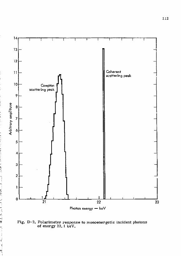
112

i4 i r

13

12

11

i r

10

I 8 D. E ° 7

-E 6 <

3

2

1 -

Compton scattering peak

Coherent scattering peak

_l_l L 22

Photon energy — keV

23

Fig. D-2. Polarimeter response to monoenergetic incident photons of energy 22. 1 keV.

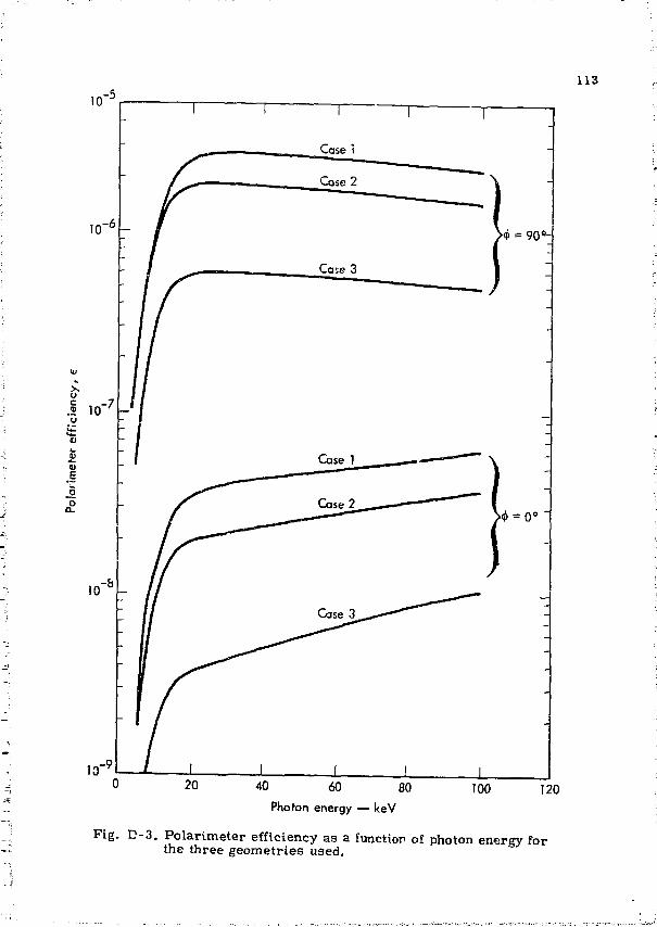
113

20 40 60 80 Photon energy — keV

100 120

Fig. D-3. Polarimeter efficiency as a function of photon energy for the three geometries used.

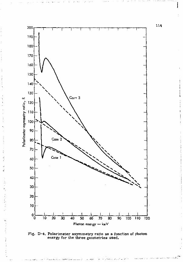
200 114

0 10 20 30 40 50 60 70 80 90 100 110 120 Photon energy — keV

Fig. D-4. Polarimeter asymmetry ratio as a function of photon energy for the three geometries used.

115

REFERENCES

1. H. S. W. Massey , E. H. S. Burhop, .nd H. B. Gilbody, E lec t ron ic and Ionic Impact Phenomena , Vol. II 'Oxford P r e s s , 1969) p. 1179 ff.

2. H. A. Bethe and E. E . Salpeter , Hanbach de r Phys ik (1957) p. 409.

3 . H. A. Bethe and L. C. Maximon, P h y s . Rev. 98, 768 (1954). 4. H. W. Koch and J . W. Motz, Rev. Mod. Phys . 3]_, 920 (1959),

F ig . 13. 5. H. K. Tseng and R. H. P r a t t , Phys . Rev. A 3, 100 (1971). 6. H. Olsen and L. C. Maximon, Phys . Rev. 114, 887 (1959). 7. C. F ronsda l and EL Ubera l l , Kiuovo C imen to 8, 163(1959) ;

P h y s . Rev. I l l , 580 (1958/. 8. A. Sommerfeld, Ann. Phys ik 11, 257 (1931). 9. P . Ki rkpa t r ick and L. Wiedmann, P h y s . Rev. 67_, 321 (1945).

10. R. L. G lucks te rn and M. H. Hull, J r . , P h y s . Rev. 90, 1030 0.953).

11. E . Haug, P h y s . Rev . 188, 63 (1969). 12. G. Elwer t , Ann. P h y s i k 34, 178 (1939). 13. R. Weinstock, P h y s . Rev. 61 , 584 (1942). 14. H. Kulenkampff, M. Scheer , and E. Z e i t l e r , Z. Phys ik 157,

275 (1959). 15. A. Sommerfeld and A . W, Maue, Ann. P h y s i k 22, 629 (1935);

W. H. F u r r y , P h y s . Rev. 46, 391 (1934). 16. M. May and G. C. Wick, Phys . Rev. j U , 628 (1951); M. May,

P h y s . Rev. 84, 265 (1951). 17. Y. F . Cheng, P h y s . Rev. 46_, 243 (1934). 18. J . W. Motz and R. C . P l ac ious , Nuovo Cimen to 15, 571 (1960). 19. G. C. Barkla , Ph i l . T r a n s . Roy. Soc. London 204, 467 (1905). 20. E. B a s s l e r , Ann. Phys ik 28, 808 (1909).

21 . L . Vegard, P r o c . Roy. Soc. London 83 , 379 (1910).

22. P. Kirkpat r ick , P h y s . Rev. J22, 226 (1923). 23. G. A. Ross , J. Opt. Soc. Am. JL6_, 375 (1928). 24. E. Wagner and P. Ott , Ann. Physik 85, 425 (1928).

116

25. W. Duane, Proc. Natl. Acad. Sci. U. S. JJj, 803 (1929). 26. H. Kulenkampff, Z. Physik 30, 513 (1929). 27. B. Dasannacharya, Phys. Rev. 3_5, 129 (1930). 28. D. S. Piston, Phys. Rev. 49, 275 (1936). 29. B. P. Boardman, Phys. Rev. 60, 163 (1941). 30. H. Kulenkampff, S. Leisegang, and M. Scheer, Z. Physik 137,

435 (1954). 31. J. W. Motz, Phys. Rev. 104, 557 (1956). 32. J. W. Motz and R. C. Placious, Phys. Rev. 112, 1039 (1958). 33. H. Kulankampff and W. Zinn, Z. Physik 161, 428 (1961). 34. F. Huffman, Linear Polarization of X-Radiation from a Mercury

Vapor Target, Ph.D. Thesis, Johns Hopkins University, Baltimore, Md. (1964).

35. M. Scheer, E. Trott, and G. Zahs, Z. Physik 209, 68 (1968). 36. V. W. Slivinsky, Bremsstrahlung Polarization from Commercial

X-Ray Tubes, Lawrence Livermore Laboratory Internal Document,. UOPE 70-9 (May 15, 1970)(avE>.ilable from the author).

37. D. R. Lasher, The Statitron,—A Low-Energy Pulsed Electron Accelerator, Lawrence Livermore Laboratory, Rept. UCRL-50215 (1967).

38. M. J. Berger and S. M. Seltzer, Tables of Energy Losses and Ranges of Electrons and Positrons, NAS-NRC Pub 1131 (1964); also NASA Rept. NASA SP-3012 (1964).

39. V. W. Cosslett and R. N. Thomas, Brit. J . Appl. Phys. ^ 1 -883 (1964).

40. E. Keil, E. Zeitler, and W. Zinn, Z. Naturforsch. 15A, 1031 (1960)[transl. in UCRL-Trans-1036 (1964)].

41. L. W. Fagg and S. S. Hanna, Rev. Mod. Phys. 3J,, 711 (1959). 42. G. J . McCallum and J . Vervier, Scintillation Spectroscopy of

Gamma Radiation, Chap. 6, Ed. 3. M. Schafroth (Gordon and Breach, New York, 1967).

43. R ; D. Evans, The Atomic Nucleus (McGraw-Hill, New York, 1955) p. 677 ff.

44. V. W. Slivinsky, Lawrence Livermore Laboratory, private cjmmunicatioa

i : 7

45. D. E. Smith, Lawrence Livermore Laboratory, private communication.

46. V. W. Slivinsky and P. J. Ebert, Nucl. Instr. Methods 71, 346 (1969).

47. P. J. Ebert, J. L. Gaines, and G. R. Leipelt, Nucl. Instr. Methods (to be published).

48. W. H. McMaster, N. Kerr DelGrande, J. H. Mallett, and J. H. Hubbell, Compilation of X-Ray Cross Sections, Lawrence Livermore Laboratory, Rept. UCRL-50174, Sec. II, Rev. 1 (1969).

49. R. W. Fink, R. C. Jopson, H. Mark, and C. D. Swift, Rev. Mod. Phys. 38, 513 (1966).

50. D. T. Keating and G. H. Vineyard, Acta. Cryst. _9, 895 (1956). 51. S. Shibata, Bull. Chem. Soc. Japan 39, 1612 (1966).

LAWRENCE LIVERMORE LABORATORY

May 15, 1972

" T TO: All holders of UCRL-51188, Linear Polarization of Low-Energy Bremsstrahlung '

FROM: Technical Information Department, L-9

ERRATA

Please make the following corrections to your copy of UCRL-51188:

Page 28 2nd paragraph, line 8 should read: " . . . N = 2 and 4, half . . . "

Page 44 Eq. (19), denominator should be: "I + I<i."

Page 91 Fig. 25, please add following legend to figure:

T = Tseng and Pra t t calculation (results available only for cases indicated by shaded regions).

S = Sommerfeld theory (Kirkpatrick and Wiedmann calculation).

S' = Relativistically-transformod Sommerfeld theory (Kulenkampff et al.).

H = Haug calculation (results available only for high-energy limit of Z = 79, T Q = 100 keV case).

i i /I Technical Information Department

l.'iersityofCalifomia RQBoxBOB Livermore.Calitomia 94550 D Telephone(415)447-1100 n Telex34-6407 AECLLLLVMR O Twx910-386-8339 AECLLLLVMR •

LAWRENCE LIVERMORE LABORATORY

May 15, 1972

TO: All holders of UCRL-51188, "Linear Polarization of Low-Energy Bremsstrahlung"

FROM: Technical Information Department, L-9

ERRATA

Please make the following corrections to your copy of UCRL-51188:

Page 28 2nd paragraph, line 8 should read: " . . . N = 2 and 4, half . . . "

Page 44 Eq. (19), denominator should be: "I + I n . "

Page 91 Fig. 25, please add following legend to figure:

T = Tseng and Prat t calculation (results available only for cases indicated by shaded regions).

S = Sommerfeld theory (Kirkpatrick and Wiedmann calculation).

S1 = Relativistically-transformed Sommerfeld theory (Kulenkampff et al.).

H = Haug calculation (results available only for high-energy limit of Z = 79, T Q = 100 keV case).

j,u/Y LiX~ H[\JUL LIL-04 (J p<}-1 i-cJ~

Technical Information Department

yasilyofCaEtoraa RO.BoxB0B Liveimore,Calitomia 94550 D Tetephane(415)447-1W0 a Telex34-6407 AEC LLL LVMR D TwxJTO-386-8339 AECLLLLVMR