Ultracold Atoms in Optical Lattices - University of Nevada, Reno

Ultracold Atoms in Optical Lattices

A thesis submitted in partial fulfillment of therequirements for the degree of Bachelor of Science in

Physics

byKiatichart Chartkunchand

Dr. Andrei Derevianko, AdvisorDr. Peter Winkler, ReaderUniversity of Nevada, Reno

May, 2006

We recommend that the thesisprepared under our supervision by

KIATTICHART CHARTKUNCHAND

entitled

Ultracold Atoms Trapped in Optical Lattices

be accepted in partial fulfilment of therequirements for the degree of

Bachelor of Science

Andrei Derevianko, Ph.D., Advisor

Peter Winkler, Ph.D., Reader

i

Abstract

Atoms can be trapped by light in the form of optical lattices, periodic structures

akin to the crystalline lattices of solid-state physics formed by the interference of

laser beams. These “light crystals” share more than just superficial looks with their

solid-state cousins: energy band structure and eigenfunctions in the form of Bloch

functions are also present in optical lattices. In this study we numerically derive

the energy bands and Bloch functions of a one-dimensional optical lattice, as well as

construct an important set of functions known as the Wannier functions which given

us a convenient basis for describing atoms trapped in these lattices. Several examples

are given of the effect on energy band structure and Wannier functions due to changes

in the parameters of the optical lattice.

ii

Acknowledgments

I would like to thank my Advisor, Dr. Andrei Derevianko, for providing me with the

necessary guidance and encouragement all throughout my research.

I would also like to thank Dr. Peter Winkler for acting as Reader for my thesis

work. I especially thank him for being able to work with me on short notice.

CONTENTS iii

Contents

Abstract i

Acknowledgments ii

List of Figures iv

1 Introduction 1

2 Theory 22.1 Optical Lattices . . . . . . . . . . . . . . . . . . . . . . . . . . . . . . 22.2 Energy Bands and Bloch Functions . . . . . . . . . . . . . . . . . . . 32.3 Wannier Functions . . . . . . . . . . . . . . . . . . . . . . . . . . . . 4

3 Procedures 63.1 Implementation of Numerov’s Method . . . . . . . . . . . . . . . . . 63.2 Determination of Allowed Energies . . . . . . . . . . . . . . . . . . . 83.3 Energies in the Harmonic Approximation . . . . . . . . . . . . . . . . 103.4 Construction of Bloch Functions . . . . . . . . . . . . . . . . . . . . . 123.5 Construction of Wannier Functions . . . . . . . . . . . . . . . . . . . 13

4 Results and Discussion 144.1 Energy Band Structure . . . . . . . . . . . . . . . . . . . . . . . . . . 144.2 Wannier Functions . . . . . . . . . . . . . . . . . . . . . . . . . . . . 154.3 Difficulties . . . . . . . . . . . . . . . . . . . . . . . . . . . . . . . . . 17

5 Conclusions 18

6 Appendix A: Source Code for “lattice.f90” 19

References 25

LIST OF FIGURES iv

List of Figures

1 Optical Lattice Potential . . . . . . . . . . . . . . . . . . . . . . . . . 22 Dispersion Curve for V0/ER = 10 (first band) . . . . . . . . . . . . . 143 Dispersion Curve for V0/ER = 200 (first band) . . . . . . . . . . . . . 144 Dispersion Curve for Different Potential Depths . . . . . . . . . . . . 145 Wannier Function for xn = 0, V0/ER = 10 . . . . . . . . . . . . . . . . 156 Wannier Function for xn = 0, V0/ER = 200 . . . . . . . . . . . . . . . 157 Wannier Function (xn = 0) for Different Potential Depths . . . . . . . 168 Comparison of w(x− xn) to Harmonic Oscillator Wavefunction . . . . 16

1 INTRODUCTION 1

1 Introduction

Optical lattices are an ideal platform for atomic experimentation. Optical lattices

have seen utilization in such diverse fields as quantum phase transitions[1] and quan-

tum computation[2]. What makes optical lattices so useful is the nearly complete

control it gives us over the system. The interaction of atoms in the lattice can easily

be control by varying the parameters of the laser being used such as the laser in-

tensity. Optical lattices are also very “clean”, that is to say that disturbances from

outside the system can be kept to a minimum. In order to utilize this important

tool, we must be able to describe the behavior of atoms trapped in these lattices in

a thorough fashion.

This study will be mainly of a computational nature. We utilize an algorithm

called Numerov’s method to numerically solve the Schrodinger equation for the po-

tential induced by the optical lattice. From the solutions we construct the energy

band structure, Bloch functions, and Wannier functions for the problem. The Bloch

functions are the eigenfunctions of the problem corresponding to the allowed energies.

Wannier functions are a set of functions derived from the Bloch functions which are

a convenient basis to represent the atoms in the lattice due to their localized nature

and property of orthogonality. To ensure the correctness of our program, we make

comparisons to the Solid State Simulation (SSS) program “Bloch”. The SSS package

is a suite of programs developed at Cornell University as a teaching and visualiza-

tion aid in the field of solid-state physics. The program “Bloch” generates the band

structure and Bloch functions for various types of potentials. We use this program

as a test case for our program, making sure that we arrive at comparable results for

the same input potentials before we proceed. More information on the SSS package,

as well as downloads, can be found at http://www.physics.cornell.edu/sss.

2 THEORY 2

2 Theory

2.1 Optical Lattices

Optical lattices act very much like the crystalline lattices of solid-state physics,

trapping atoms at the minima of the overall potential. In this work we consider

a one-dimensional optical lattice, constructed from the interference of two counter-

propagating laser beams with orthogonal polarizations. Consider the two laser beams

to be monochromatic plane waves of frequency ω; then the resulting electric field is

given by:

E(x, t) = E+(x, t)ε+e−iωt + E−(x, t)ε−e−iωt.

Here E±(x, t) = E0e±ikLx, where kL ≡ 2π/λ is the wavenumber of the laser, and ε± is

the polarization vector. The potential V (x) felt by atoms in the lattice is proportional

to |E±(x, t)|2[3]: V (x) ∝ cos2(kx). A more convenient parametrization leads us to

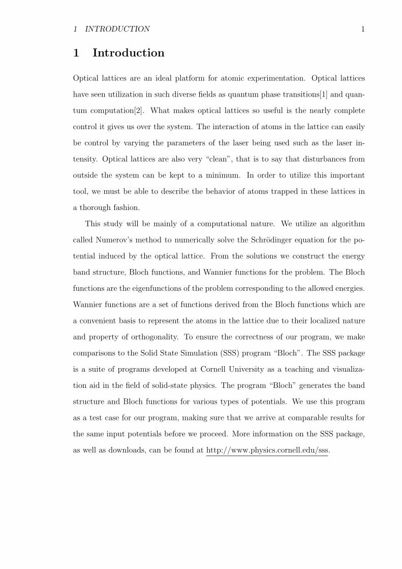
the form of the potential we will use throughout this work: V (x) = V0 sin2(πax), where

a ≡ λ/2 is the periodicity of the lattice.

Figure 1: Optical Lattice Potential

Trapping of atoms within the lattice is

achieved by an effect known as “Sisyphus

cooling”. We note that by having the two

opposing laser beams be of orthogonal polar-

ization to each other, the resulting polariza-

tion rotates in space: the polarization is lin-

ear at x = 0, λ/4, λ/2, . . ., clockwise circular

at x = λ/8, 5λ/8, . . ., and counter-clockwise

circular at x = 3λ/8, 7λ/8, . . .[4]. The elec-

tric field generated by the lasers causes a

shift in the energy levels of the atom due to the AC Stark effect, an electrical ana-

2 THEORY 3

logue to the Zeeman effect. Suppose an atom has two degenerate sublevels to its

ground state. These levels will oscillate in space in accordance with the polarization,

with one sublevel experiencing the largest shift at a point of clockwise circular po-

larization and the other at a point of counter-clockwise circular polarization[4]. The

result is that once atoms traveling along the potential wells of one of the sublevels

reach the top of those wells, they are optically pump to the bottom of the potential

well of the other sublevel and lose energy in the process[4]. Eventually the atoms do

not have enough energy to get over the potential hill and remain trapped around the

potential minima of each lattice site.

2.2 Energy Bands and Bloch Functions

For this work, we have recourse to solving the one-dimensional, time-independent

Schrodinger equation for a periodic potential:

−~2

2m

d2ψ

dx2+ V (x)ψ(x) = Eψ(x),

V (x) = V0 sin2(π

ax)

,

where a ≡ λ2

is the period of the potential. Solutions for this particular class of

potentials are governed by Bloch’s theorem, which states that:

ψk(x) = uk(x)eikx, (1)

where the function uk(x) has the periodicity of the lattice and k, the wavenumber,

is real. This results in what are called Bloch functions, eigenfunctions of the Hamil-

tonian for this system. Thus by solving the problem in one particular cell of the

potential, we can derive the wavefunction in other cells by applying Bloch’s theorem.

2 THEORY 4

A particular characteristic of periodic potentials is the notion of allowed and

forbidden energies. Allowed energies are those that correspond to the Bloch functions.

These allowed ranges of E are separated by gaps corresponding to forbidden energies,

values of E which result in solutions of the same form as (1) but with imaginary

values of k. Thus the forbidden energies correspond to solutions with an exponential

behavior. This series of allowed and forbidden energies is called the band structure

of the lattice in question.

2.3 Wannier Functions

Bloch functions give us the solution to Schrodinger’s equation for the given periodic

potential; it would be of great use, however, to derive a complete set of orthonormal

functions which are localized about each potential minima. These set of functions

are know as Wannier functions. For a given energy band l, the Wannier functions are

defined by the Bloch functions as (in one dimension)[5]:

wl(x− xn) = N−1/2∑

k

exp{−ikxn}ψlk(x), (2)

where xn = na is a lattice site position with n ∈ Z and N is the number of lattice

points where we consider N atoms on a string with the ends connected so as to obtain

periodic boundary conditions. We show that Wannier functions are orthonormal in

the following manner:

∫w∗

l (x− xn)wl′(x− xn′)dx =1

N

∫[∑

k

eikxnψ∗lk(x)][∑

k′e−ik′xn′ψl′k′(x)]dx

=1

N

∑

k,k′eikxne−ik′xn′

∫ψ∗lk(x)ψl′k′(x)dx

=1

N

∑

k,k′eikxne−ik′xn′δkk′δll′

2 THEORY 5

=1

N

∑

k

eik(xn−xn′ )δll′

= δxnxn′δll′ .

For this study we adopt a continuous limit of the Wannier functions by noting that∑

k → Na2π

∫ π/a

−π/adk. This comes from considering our system to be a string of N

atoms. The limits of integration contain the first Brillioun zone, where the relevant

values of k reside; outside of this the values repeat those within the first Brillioun

zone due to the periodicity of the lattice. We also concentrate on only one particular

energy band (the first band), so we drop the band index l from the Wannier function

and end up with:

w(x− xn) =

√a

2π

∫ π/a

−π/a

exp{−ikxn}ψk(x)dk. (3)

There is a certain ambiguity to the definition of the Wannier functions due to

phase of the Bloch functions not being defined. To ensure that the corresponding

Wannier functions are real and symmetric about each lattice point, we require that

ψk(x = 0) is real and continuous for all allowed k[6]. To ensure this amounts to

multiplying the Bloch functions by a phase factor such that:

ψk(x) → exp{−i arg[ψk(0)]}ψk(x), (4)

where arg[ψk(0)] = tan−1{=[ψk(0)]/<[ψk(0)]}.

3 PROCEDURES 6

3 Procedures

3.1 Implementation of Numerov’s Method

Numerov’s method[7] is an efficient numerical algorithm for solving differential equa-

tions of the same form as Schrodinger’s equation, i.e. second-order linear ordinary

differential equations which do not depend on the first derivative. Let xn ≡ x0 + nh

where x0 is the starting point of integration and h is the step size. If we re-write

Schrodinger’s equation in the form:

ψ′′ +2m

~2[E − V (x)]ψ = 0,

Numerov’s method gives us[7]:

ψn+1(12− h2Vn+1) + ψn(−24− 10h2Vn) + ψn−1(12− h2Vn−1)

= −h2E(ψn+1 + 10ψn + ψn−1) + O(h6),

where ψn ≡ ψ(xn) and Vn ≡ V (xn). If we now let k2 ≡ E − V (x) and solve for ψn+1,

we arrive at:

ψn+1 =2(1− 5h2

12k2

n)ψn − (1 + h2

12k2

n−1)ψn−1

1 + h2

12k2

n+1

+ O(h6), (5)

where k2n ≡ k2(xn). This is the form of Numerov’s method that is implemented

in the program. From the above algorithm, we can see that each new solution is

calculated from the two previous solutions. Thus to begin the process, we would

require knowledge of ψ0 and ψ1. This then begs the question: How do we begin the

Numerov algorithm? One method would be use ψ0 in another method such as the

classic Runge-Kutta algorithm to determine ψ1 and then continue with the Numerov

3 PROCEDURES 7

algorithm from there. The method[8] we use in this study, however, is to use an

explicit expression for ψ1. First we re-write the Schrodinger equation in the form:

d2ψ

dx2= U(x)ψ,

where U(x) ≡ 2m~2 [V0 sin2(π

ax) − E] and let F ≡ U(x)ψ. Then, with knowledge of ψ0

and ψ′0, it can be shown that[8]:

ψ1 =ψ0(1− U2h2

24) + hψ′0(1− U2h2

12) + 7h2

24F0 − U2h4

36F0

1− U1h2

4+ U1U2h4

18

. (6)

ψ1 is calculated to an accuracy O(h5), which ensures that ψ2 will be calculated O(h6)

since the global error of Numerov’s method is O(h5) and we only calculate ψ1 once.

In applying Numerov’s method to the problem, we first realize that since we are

dealing with a second-order ordinary differential equation we can express the general

solution ψk(x) as a combination of two linearly independent solutions of the equation,

φ1(x) and φ2(x):

ψk(x) = C1φ1(x) + C2φ2(x).

For comparison with the SSS “Bloch” program, we adopt the following boundary

conditions on φ1(x) and φ2(x):

φ1

(−a

2

)= 1, φ′1

(−a

2

)= 0,

φ2

(−a

2

)= 0, φ′2

(−a

2

)=

1

a,

where a is the lattice constant of the potential. Numerov’s method is used to de-

termine both φ1(x) and φ2(x). We concentrate on a unit cell of the optical lattice

centered around x = 0, corresponding to an integration interval of −a/2 < x < a/2.

3 PROCEDURES 8

3.2 Determination of Allowed Energies

Once φ1(x) and φ2(x) have been determined for a given energy value E, we can

determine if E is an allowed energy. First let us utilize the boundary conditions

defined above in ψk(x):

ψk

(−a

2

)= C1φ1

(−a

2

)+ C2φ2

(−a

2

)= C1,

ψ′k(−a

2

)= C1φ

′1

(−a

2

)+ C2φ

′2

(−a

2

)=

1

aC2.

At the endpoints of the interval, we have ψk(−a/2) = uk(−a/2)e−ika/2 and ψk(a/2) =

uk(a/2)eika/2 by application of Bloch’s theorem. Since uk(−a/2) = uk(a/2) due to

the periodicity of uk(x), we end up having ψk(a/2) = eikaψk(−a/2). From this we

obtain the equations:

ψk

(a

2

)= eikaψk

(−a

2

)= eikaC1,

ψ′k(a

2

)= eikaψ′k

(−a

2

)=

a

2eikaC2.

To solve for the constants C1 and C2, we end up with a system of linear equations in

C1 and C2. We can re-arrange the equations as follows:

[φ1

(a

2

)− eika

]C1 + φ2

(a

2

)C2 = 0,

φ′1(a

2

)C1 +

[φ′2

(a

2

)− 1

aeika

]C2 = 0.

For a non-trivial solution to the above system, the determinant of the system must

be equal to zero. Thus:

det =

∣∣∣∣∣∣∣φ1

(a2

)− eika φ2

(a2

)

φ′1(

a2

)φ′2

(a2

)− 1aeika

∣∣∣∣∣∣∣= 0

3 PROCEDURES 9

=[φ1

(a

2

)− eika

] [φ′2

(a

2

)− 1

aeika

]− φ′1

(a

2

)φ2

(a

2

)

= φ1

(a

2

)φ′2

(a

2

)− φ′1

(a

2

)φ2

(a

2

)+

1

a

(eika

)2 − eikaφ′2(a

2

)− 1

aeikaφ1

(a

2

).

We recognize the term φ1φ′2 − φ′1φ2 as the Wronskian for this problem, defined as:

W (x) =

∣∣∣∣∣∣∣φ1(x) φ2(x)

φ′1(x) φ′2(x)

∣∣∣∣∣∣∣.

For a differential equation of the form y′′ + P (x)y′ + Q(x)y = 0, the Wronskian is

given by Abel’s formula as:

W (x) = W (x0) exp{∫ x

x0

P (x)dx}.

Since the Schrodinger equation is of the required form and is independent of the first

derivative, P (x) = 0 and thus W (x) = W (x0). This implies that the Wronskian is

independent of x and we can use its known value at W (x = −a/2). When we evaluate

the Wronskian at x = −a/2, we find that W (−a/2) = 1/a. Plugging this into (6),

we arrive at the characteristic equation:

λ2 −[aφ′2

(a

2

)+ φ1

(a

2

)]λ + 1 = 0, (7)

where λ ≡ eika. Solutions to this equation take the form of:

λ1,2 = eika =1

2

[φ1

(a

2

)+ aφ′2

(a

2

)]± i

√1− 1

4

[φ1

(a

2

)+ aφ′2

(a

2

)]2

. (8)

Defining Q ≡ 12[φ1(a/2) + aφ′2(a/2)], if |Q| ≤ 1 we end up with the situation where k

is real, resulting in :

k =1

acos−1 Q. (9)

3 PROCEDURES 10

In this case the energy value E used to solve for φ1(x) and φ2(x) is one of the allowed

energy values and will correspond to a particular Bloch function.

To determine the overall band structure of the optical lattice, we begin with an

energy of 0 and work our way up to the potential height using a prescribed energy

step size, testing whether the particular value yields a result of |Q| ≤ 1.

3.3 Energies in the Harmonic Approximation

We can obtain an estimate for the energy of the first band of the lattice by approx-

imating it with a harmonic oscillator potential. We begin by introducing a scaled

form of Schrodinger’s equation for the problem. Consider the Schrodinger equation

for this problem:

ψ′′k(x) =2m

~2

[V0 sin2

(π

ax)− E

]ψk(x).

We introduce a dimensionless parameter ξ ≡ xa

and re-write the equation as:

ψ′′k(ξ) =2ma2

~2

[V0 sin2(πξ)− E

]ψk(ξ).

Next we introduce the photon recoil energy ER ≡ ~2k2/2m and multiply the right-

hand side of the above equation by the factor ER/ER:

ψ′′k(ξ) =2ma2

~2ER

[V0

ER

sin2(πξ)− E

ER

]ψk(ξ)

=2ma2

~2

(~2k2

2m

)[V0

ER

sin2(πξ)− E

ER

]ψk(ξ)

= a2k2

[V0

ER

sin2(πξ)− E

ER

]ψk(ξ)

= a2(π

a

)2[

V0

ER

sin2(πξ)− E

ER

]ψk(ξ)

= [V S sin2(πξ)− ES]ψk(ξ).

3 PROCEDURES 11

Here we have introduced the dimensionless parameters V S ≡ π2V0/ER and ES ≡π2E/ER. This scaling effectively gives us position in units of the lattice constant a

and energy in units of the photon recoil energy ER.

We now apply the harmonic approximation by taking a Taylor expansion of the

scaled potential V (ξ) = V S sin2(πξ) about the potential minimum at ξ = 0. For a

lattice with a sufficiently deep potential, we can neglect terms involving powers of ξ

greater than two and end up with:

V S sin2(πξ) ≈ V Sπ2ξ2.

Equating this to the potential of a harmonic oscillator, we arrive at:

V Sπ2ξ2 =mω2a2ξ2

2ER

,

where we have taken care to scale the harmonic oscillator potential in the same manner

as we did the Schrodinger equation. We now solve for ω:

ω2 =2ERπ2

ma2V S

=2π2

ma2

(~2k2

2m

)V S

ω =π2~ma2

√V S.

The ground-state energy of a harmonic oscillator is given by E0 = 12~ω. Using our

expression for ω we obtain:

E0 =1

2~

(π2~ma2

√V S

)

=π2~2

2ma2

√V S

3 PROCEDURES 12

= ER

√V S.

We now have an estimate for the energy of the first band of the lattice. Letting

ESest ≡ E0/ER, we finally have:

ESest =

√V S = π

√V0

ER

. (10)

3.4 Construction of Bloch Functions

Now that we have the allowed values for E and k, we can determined the Bloch

functions ψk(x). Knowing the value of k helps us in determining the constants C1 and

C2 which are involved the the construction of ψk(x) from the two linearly independent

solutions φ1(x) and φ2(x) of Schrodinger’s equation. Setting C1 = 1 for the time being

(we will fix it by normalization later), we solve one of our equations from the system

in the previous section for C2:

[φ1

(a

2

)− eika

]C1 + φ2

(a

2

)C2 = 0,

[φ1

(a

2

)− eika

]+ φ2

(a

2

)C2 = 0,

C2 =1

φ2

(a2

)[eika − φ1

(a

2

)]. (11)

We now have our Bloch functions determined by the linear combination of φ1(x) and

φ2(x):

ψk(x) = φ1(x) + C2φ2(x), (12)

with C2 given in (11).

There is still the matter of normalization and fixing the phase of the Bloch func-

tions. For comparison with the SSS “Bloch” program, we normalize the Bloch func-

3 PROCEDURES 13

tions in the following manner:

N =1

a

∫ a/2

−a/2

|ψk(x)|2 dx.

We fix the phase by requiring ψk(x = 0) to be real and continuous. Thus our final

Bloch functions will take the form:

ψk(x) → 1√N

exp{−i arg[ψk(0)]}ψk(x). (13)

3.5 Construction of Wannier Functions

With the Bloch functions determined for a particular energy band, we can now deter-

mine the Wannier functions. Recall that the Wannier functions are defined in terms

of the Bloch functions by:

w(x− xn) =

√a

2π

∫ π/a

−π/a

exp{−ikxn}ψk(x)dk.

We begin by constructing the Wannier function for xn = 0; the functions about other

lattice points are given by simple translations of the one about xn = 0. By the very

nature of our program for constructing Bloch functions, we are limited to the unit cell

about xn = 0, i.e. in the interval −a/2 < x < a/2. Thus an initial determination of

the Wannier function would give us the function in that interval. To find the Wannier

function in a large enough interval where we can verify the exponential decay of the

function, we determine the Wannier function about other lattice points while still

looking through our restricted interval. For example, by determining w(x− a), what

we would see in our unit interval would be the function value of w(x−0) in the interval

−3a/2 < x < −a/2; similarly determining the Wannier function about xn = −a, we

would give us the function about xn = 0 in the interval a/2 < x < 3a/2.

4 RESULTS AND DISCUSSION 14

4 Results and Discussion

4.1 Energy Band Structure

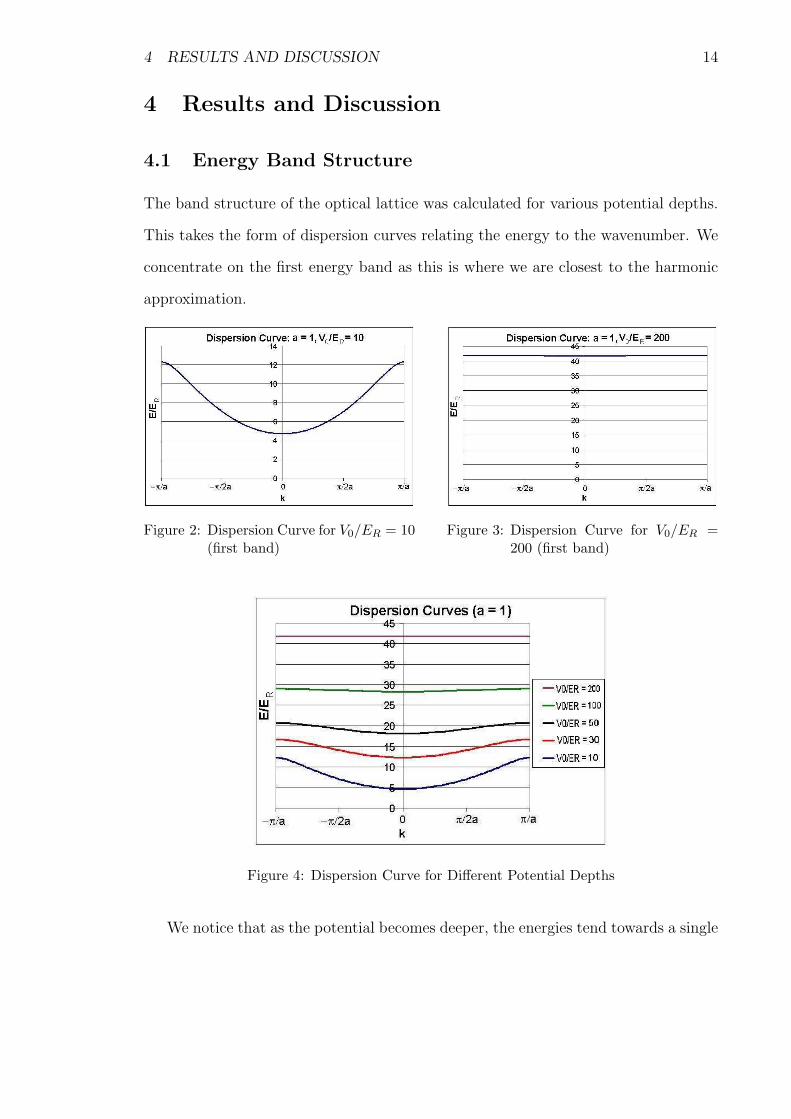
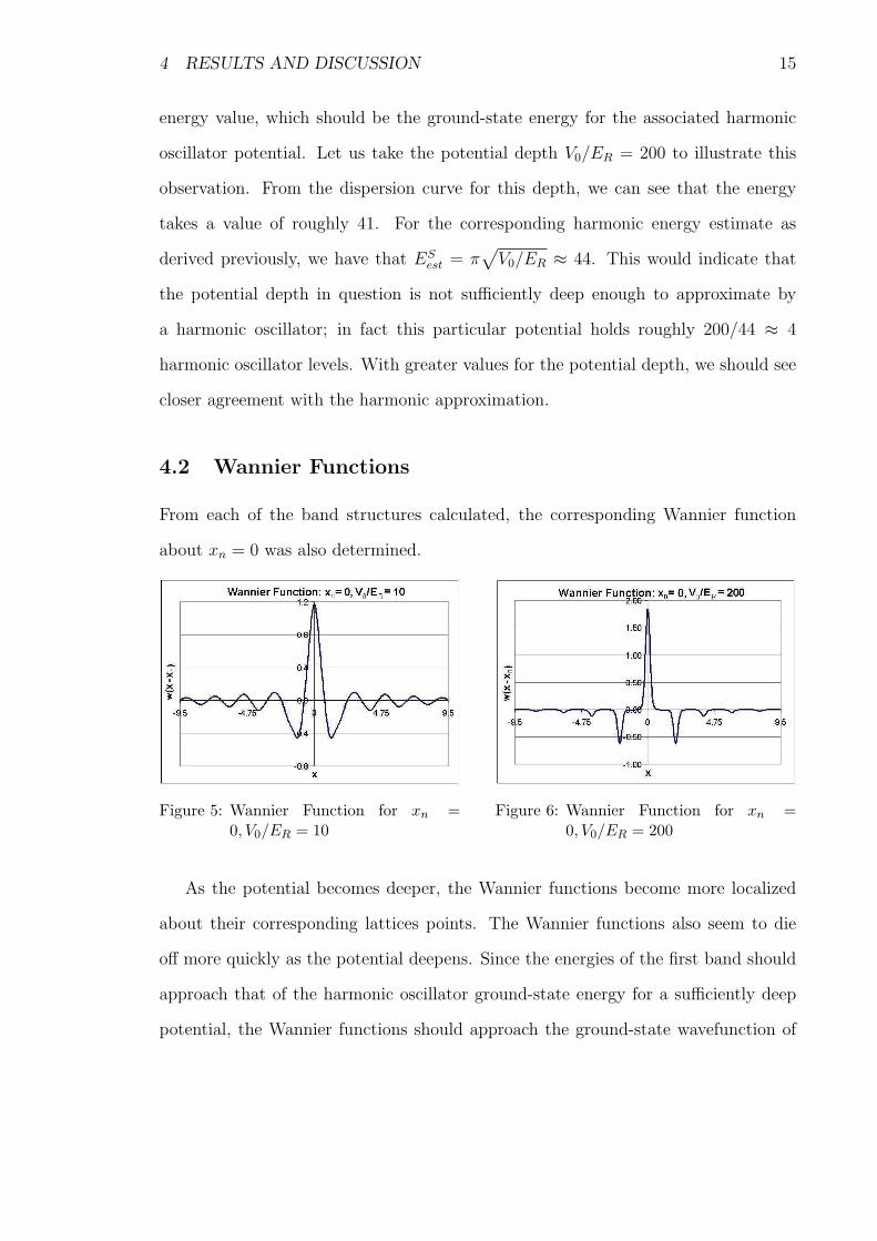
The band structure of the optical lattice was calculated for various potential depths.

This takes the form of dispersion curves relating the energy to the wavenumber. We

concentrate on the first energy band as this is where we are closest to the harmonic

approximation.

Figure 2: Dispersion Curve for V0/ER = 10(first band)

Figure 3: Dispersion Curve for V0/ER =200 (first band)

Figure 4: Dispersion Curve for Different Potential Depths

We notice that as the potential becomes deeper, the energies tend towards a single


energy value, which should be the ground-state energy for the associated harmonic

oscillator potential. Let us take the potential depth V0/ER = 200 to illustrate this

observation. From the dispersion curve for this depth, we can see that the energy

takes a value of roughly 41. For the corresponding harmonic energy estimate as

derived previously, we have that ESest = π

√V0/ER ≈ 44. This would indicate that

the potential depth in question is not sufficiently deep enough to approximate by

a harmonic oscillator; in fact this particular potential holds roughly 200/44 ≈ 4

harmonic oscillator levels. With greater values for the potential depth, we should see

closer agreement with the harmonic approximation.

4.2 Wannier Functions

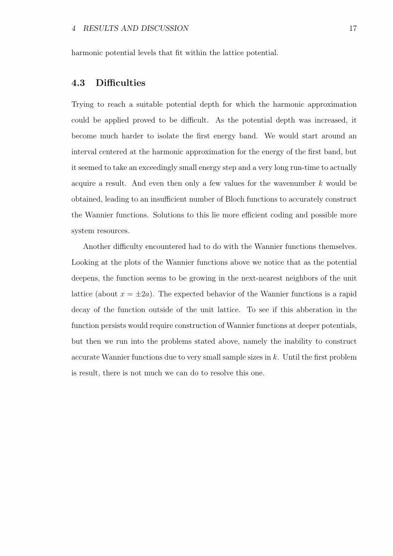
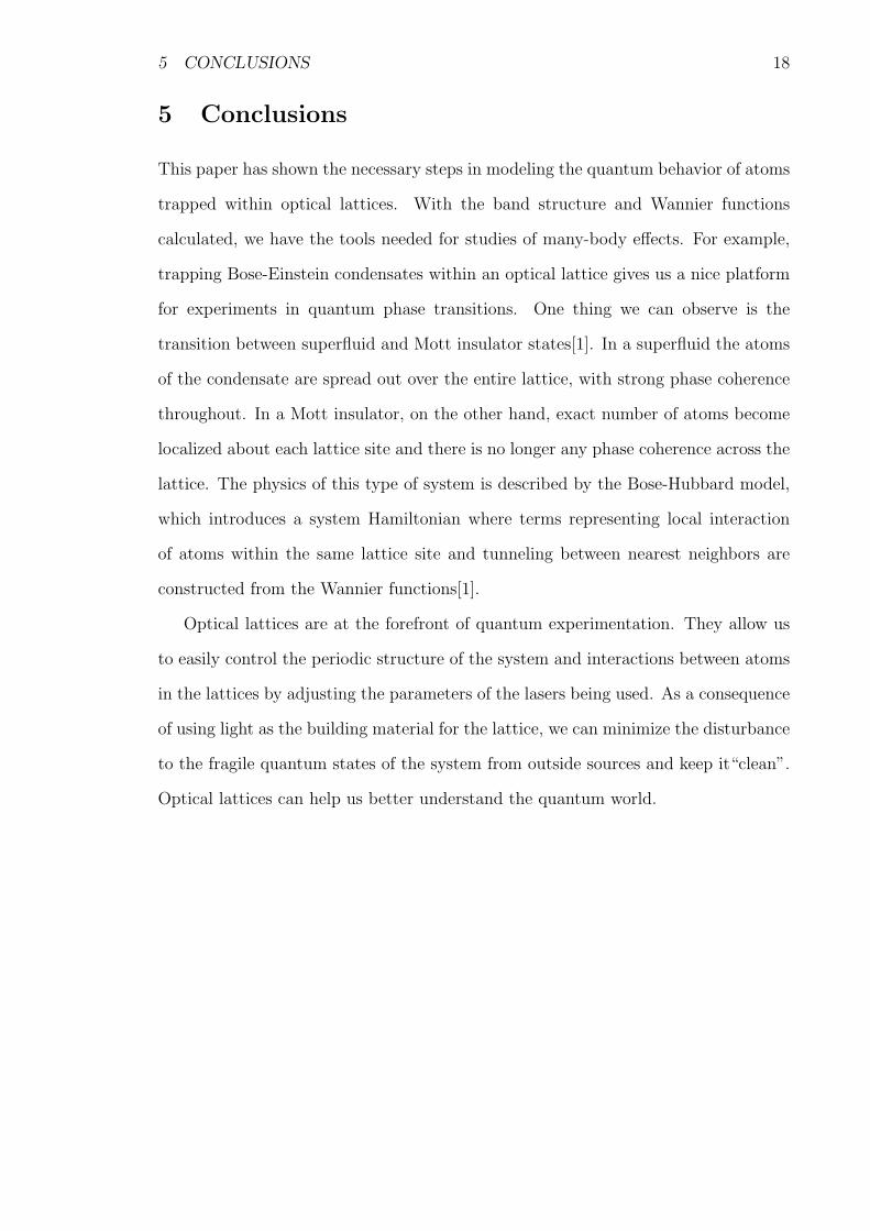
From each of the band structures calculated, the corresponding Wannier function

about xn = 0 was also determined.

Figure 5: Wannier Function for xn =0, V0/ER = 10

Figure 6: Wannier Function for xn =0, V0/ER = 200

As the potential becomes deeper, the Wannier functions become more localized

about their corresponding lattices points. The Wannier functions also seem to die

off more quickly as the potential deepens. Since the energies of the first band should

approach that of the harmonic oscillator ground-state energy for a sufficiently deep

potential, the Wannier functions should approach the ground-state wavefunction of


Figure 7: Wannier Function (xn = 0) for Different Potential Depths

the harmonic oscillator given by: ψHO(x) = (mω/π~)1/4 exp{−12

mω~ x2}.

Figure 8: Comparison of w(x− xn) to Harmonic Oscillator Wavefunction

We see that the Wannier function in this case is noticeably different from the

harmonic oscillator wavefunction. This we expect since we found that the particular

potential depth this Wannier function is defined for is not deep enough to be approxi-

mated by a harmonic oscillator. That the Wannier function is less than the harmonic

oscillator wavefunction makes sense in this case since it is spread over the four or so


harmonic potential levels that fit within the lattice potential.

4.3 Difficulties

Trying to reach a suitable potential depth for which the harmonic approximation

could be applied proved to be difficult. As the potential depth was increased, it

become much harder to isolate the first energy band. We would start around an

interval centered at the harmonic approximation for the energy of the first band, but

it seemed to take an exceedingly small energy step and a very long run-time to actually

acquire a result. And even then only a few values for the wavenumber k would be

obtained, leading to an insufficient number of Bloch functions to accurately construct

the Wannier functions. Solutions to this lie more efficient coding and possible more

system resources.

Another difficulty encountered had to do with the Wannier functions themselves.

Looking at the plots of the Wannier functions above we notice that as the potential

deepens, the function seems to be growing in the next-nearest neighbors of the unit

lattice (about x = ±2a). The expected behavior of the Wannier functions is a rapid

decay of the function outside of the unit lattice. To see if this abberation in the

function persists would require construction of Wannier functions at deeper potentials,

but then we run into the problems stated above, namely the inability to construct

accurate Wannier functions due to very small sample sizes in k. Until the first problem

is result, there is not much we can do to resolve this one.

5 CONCLUSIONS 18

5 Conclusions

This paper has shown the necessary steps in modeling the quantum behavior of atoms

trapped within optical lattices. With the band structure and Wannier functions

calculated, we have the tools needed for studies of many-body effects. For example,

trapping Bose-Einstein condensates within an optical lattice gives us a nice platform

for experiments in quantum phase transitions. One thing we can observe is the

transition between superfluid and Mott insulator states[1]. In a superfluid the atoms

of the condensate are spread out over the entire lattice, with strong phase coherence

throughout. In a Mott insulator, on the other hand, exact number of atoms become

localized about each lattice site and there is no longer any phase coherence across the

lattice. The physics of this type of system is described by the Bose-Hubbard model,

which introduces a system Hamiltonian where terms representing local interaction

of atoms within the same lattice site and tunneling between nearest neighbors are

constructed from the Wannier functions[1].

Optical lattices are at the forefront of quantum experimentation. They allow us

to easily control the periodic structure of the system and interactions between atoms

in the lattices by adjusting the parameters of the lasers being used. As a consequence

of using light as the building material for the lattice, we can minimize the disturbance

to the fragile quantum states of the system from outside sources and keep it“clean”.

Optical lattices can help us better understand the quantum world.

6 APPENDIX A: SOURCE CODE FOR “LATTICE.F90” 19

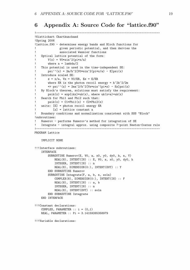
6 Appendix A: Source Code for “lattice.f90”

!--------------------------------------------------------------------------!Kiattichart Chartkunchand!Spring 2006!lattice.f90 - determines energy bands and Bloch functions for! given periodic potential, and then dervies the! associated Wannier functions! Optical lattice potential of the form:! V(x) = V0*sin^2(pi*x/a)! where a = lambda/2! This potential is used in the time-independent SE:! psi’’(x) = 2m/h^2[V0*sin^2(pi*x/a) - E]psi(x)! Introduce scaled SE:! z = x/a, Vs = V0/ER, Es = E/ER! where ER is the photon recoil energy = h^2k^2/2m! => psi’’(z) = 2ma^2/h^2[Vs*sin^(pi*z) - Es]psi(z)! By Bloch’s theorem, solutions must satisfy the requirement:! psik(x) = exp{ikx}*uk(x), where uk(x+a)=uk(x)! Search for Phi1 and Phi2 such that:! psik(x) = C1*Phi1(x) + C2*Phi2(x)! units: [E] = photon recoil energy ER! [x] = lattice constant a! Boundary conditions and normalization consistent with SSS "Bloch"!subroutines:! Numerov - performs Numerov’s method for integration of SE! Integrate - integral approx. using composite 7-point Newton-Coates rule!--------------------------------------------------------------------------PROGRAM Lattice

IMPLICIT NONE

!!!Interface subroutines:INTERFACE

SUBROUTINE Numerov(E, V0, a, x0, y0, dy0, h, n, Y)REAL(8), INTENT(IN) :: E, V0, a, x0, y0, dy0, hINTEGER, INTENT(IN) :: nREAL(8), DIMENSION(0:), INTENT(OUT) :: Y

END SUBROUTINE NumerovSUBROUTINE Integrate(F, a, b, n, soln)

COMPLEX(8), DIMENSION(0:), INTENT(IN) :: FREAL(8), INTENT(IN) :: a, bINTEGER, INTENT(IN) :: nREAL(8), INTENT(OUT) :: soln

END SUBROUTINE IntegrateEND INTERFACE

!!!Constant declarations:COMPLEX, PARAMETER :: i = (0,1)REAL, PARAMETER :: Pi = 3.14159265358979

!!!Variable declarations:


COMPLEX(8) :: C, phaseCOMPLEX(8), DIMENSION(:), ALLOCATABLE :: Psi, W, TempCOMPLEX(8), DIMENSION(:,:), ALLOCATABLE :: blochTblREAL(8) :: Es, dE, Vs, y10, dy10, y20, dy20, Step, Xmin, Xmax, x0, a, &

Q, dPhi2, xi, k, soln, Emin, Emax, kmin, kmax, argREAL(8), DIMENSION(:), ALLOCATABLE :: Phi1, Phi2REAL(8), DIMENSION(:,:), ALLOCATABLE :: DispINTEGER :: Points, Nodes, j, l, m, n, p, r, s, OpenStat, mid, numk, &

InputStatus, knum

!!!Create files to write to:OPEN(UNIT = 2, FILE = "dispCurve.dat", STATUS = "REPLACE", ACTION = &

"WRITE", IOSTAT = OpenStat)OPEN(UNIT = 4, FILE = "wannier.dat", STATUS = "REPLACE", ACTION = &

"WRITE", IOSTAT = OpenStat)!!!Determine allowed energies (first band only):

!!!declare lattice constant and integration range:a = 1Xmin = -a/2Xmax = a/2!!!declare grid and step size:Points = 2100Step = (Xmax-Xmin)/Pointsmid = (Points/2)+1!!!allocate arrays:ALLOCATE(Phi1(0:Points), Phi2(0:Points), Psi(0:Points), Temp(0:Points))!!!declare boundary conditions:x0 = Xminy10 = 1.0dy10 = 0.0y20 = 0.0dy20 = 1/a!!!declare energy bounds, energy step, and potential strength:Emin = 28.0Emax = 30.0dE = 0.001Vs = 100.0!!!find number of allowed energies:WRITE(*,*), "Looking for allowed energies..."Es = Eminnumk = 0DO WHILE(Es <= Emax)

!!!integrate Phi1:CALL Numerov(Es,Vs,a,x0,y10,dy10,Step,Points,Phi1)!!!integrate Phi2:CALL Numerov(Es,Vs,a,x0,y20,dy20,Step,Points,Phi2)!!!check for allowed energy:!!!numerical estimate of derivative Phi2 at a/2:dPhi2 = (11*Phi2(Points)-18*Phi2(Points-1)+9*Phi2(Points-2)- &

2*Phi2(Points-3))/(6*Step)Q = 0.5*(Phi1(Points) + a*dPhi2)IF(ABS(Q) <= 1) THEN


k = ACOS(Q)/aWRITE(2,*), k, Esnumk = numk + 1

END IF!!!increase energy by dE:Es = Es + dE

END DOWRITE(*,*), numk, " allowed energies found"CLOSE(2)!!!write to dispCurve (-k -> k):ALLOCATE(Disp(0:2*numk+1,0:1))OPEN(UNIT = 2, FILE = "dispCurve.dat", STATUS = "OLD", ACTION = &

"READ", IOSTAT = OpenStat)n = numk - 1m = numkDO

READ(2,*,IOSTAT=InputStatus), k, EsIF(InputStatus < 0) EXITDisp(n,0) = -kDisp(n,1) = EsDisp(m,0) = kDisp(m,1) = Esn = n - 1m = m + 1

END DOCLOSE(2)OPEN(UNIT = 2, FILE = "dispCurve.dat", STATUS = "REPLACE", ACTION = &

"WRITE", IOSTAT = OpenStat)n = numk - 1DO n = 0, 2*numk-1

WRITE(2,*), Disp(n,0), Disp(n,1)END DOCLOSE(2)

!!!Determine Wannier function about x = 0:WRITE(*,*), "Determining Wannier function about x = 0..."knum = 2*numk+1s = 19*Points + 18!!!allocate arrays:ALLOCATE(blochTbl(0:knum,0:Points), W(0:s))!!!determine Bloch functions from x = -9a -> 9a:p = 0Xmin = -19*a/2DO j = 9, -9, -1

Xmax = Xmin + aWRITE(*,*), "*"!!!open file to read from:OPEN(UNIT = 2, FILE = "dispCurve.dat", STATUS = "OLD", ACTION = &

"READ", IOSTAT = OpenStat)DO m = 0, knum

!!!read allowed energy from file:READ(2,*,IOSTAT=InputStatus), k, Es


IF(InputStatus < 0) EXIT!!!integrate Phi1:CALL Numerov(Es,Vs,a,x0,y10,dy10,Step,Points,Phi1)!!!integrate Phi2:CALL Numerov(Es,Vs,a,x0,y20,dy20,Step,Points,Phi2)!!!determine Bloch function:C = (EXP(i*k*a) - Phi1(Points))/Phi2(Points)Psi = Phi1 + C*Phi2!!!determine normalization and appropriate phase factor:Temp = ABS(Psi)**2CALL Integrate(Temp,Xmin,Xmax,Points,soln)arg = ATAN2(AIMAG(Psi(mid)),REAL(Psi(mid)))phase = EXP(-i*arg)Psi = a*phase*Psi/SQRT(soln)DO n = 0, Points

blochTbl(m,n) = EXP(-i*k*j*a)*Psi(n)END DO

END DODEALLOCATE(Temp)ALLOCATE(Temp(0:knum))!!!calculate Wannier function:r = 0kmin = -Pi/akmax = Pi/aDO n = p*Points+p, (p+1)*Points+p

DO m = 0, knumTemp(m) = blochTbl(m,r)

END DOCALL Integrate(Temp,kmin,kmax,knum,soln)W(n) = solnr = r + 1

END DODEALLOCATE(Temp)ALLOCATE(Temp(0:Points))p = p + 1CLOSE(2)Xmin = Xmax

END DOWRITE(*,*), "Wannier function found!"Xmin = -19*a/2Xmax = 19*a/2Step = (Xmax-Xmin)/sx0 = XminDO n = 0, s

xi = x0 + n*StepWRITE(4,*), xi, REAL(W(n))

END DO

END PROGRAM Lattice


!--------------------------------------------------------------------------!subroutine Numerov: implements Numerov’s method!for y’’ = U(x) + V(x)y:! let F = U(x) + V(x)y! for SE -! in SSS "Bloch": y’’ = (2m/h^2)[V(x) - E]y! in scaled units: y’’ = (2ma^2/h^2)[V(x) - E]y! => U(x) = 0, V(x) = (2ma^2/h^2)[V(x) - E]! => F = (2ma^2/h^2)[V(x) - E]y! for comparison with SSS "Bloch": 2m/h^2 = 0.262465!input:! E - estimate of eigenenergy! V0 - strength of potential! a - lattice constant! x0 - starting point of integration! y0 - value of wavefunction at starting point of integration! dy0 - derivative of wavefunction at starting point of integration! h - step size! n - number of grid points! Y - array holding values of wavefunction at grid points!output:! Y - array representing solution to SE for given E!***equation for y1 derived in:! "Getting Started With Numerov’s Method"! J.L.M. Quiroz Gonzalez and D. Thompson! Computers in Physics, Vol. 11, No. 5, Sep/Oct 1997!--------------------------------------------------------------------------SUBROUTINE Numerov(E, V0, a, x0, y0, dy0, h, n, Y)

IMPLICIT NONE

REAL, PARAMETER :: Pi = 3.14159265358979REAL(8), INTENT(IN) :: E, V0, a, x0, y0, dy0, hINTEGER, INTENT(IN) :: nREAL(8), DIMENSION(0:), INTENT(OUT) :: YREAL(8) :: F, k2(0:n), C1, C2, C3, C4, C5, xi, V1, V2, V3INTEGER :: i

C1 = h**2 / 24C2 = h**2 / 12C3 = h**4 / 36C4 = h**2 / 4C5 = h**4 / 18V1 = V0*SIN(Pi*x0/a)**2 - EV2 = V0*SIN(Pi*(x0+h)/a)**2 - EV3 = V0*SIN(Pi*(x0+2*h)/a)**2 - EY(0) = y0F = V1*Y(0)

!!!compute value for y1:Y(1) = (Y(0)*(1-C1*V3) + h*dy0*(1-C2*V3) + 7*C1*F - C3*F*V3)/ &

(1 - C4*V2 + C5*V2*V3)!!!implement Numerov’s method:


DO i = 0, nxi = x0 + i*hk2(i) = E-V0*SIN(Pi*xi/a)**2

END DODO i = 1, n-1

Y(i+1) = (2*(1-5*C2*k2(i))*Y(i) - (1+C2*k2(i-1))*Y(i-1))/ &(1+C2*k2(i+1))

END DO

END SUBROUTINE Numerov

!--------------------------------------------------------------------------!subroutine Integrate: integral approximation using composite! 7-point Newton-Coates rule!input:! soln - variable to hold value of integration! a - lower limit of integration! b - upper limit of integration! n - number of points in integration interval! F - array containing function values to integrate!output:! soln - value of integration!--------------------------------------------------------------------------SUBROUTINE Integrate(F, a, b, n, soln)

IMPLICIT NONE

COMPLEX(8), DIMENSION(0:), INTENT(IN) :: FREAL(8), INTENT(IN) :: a, bINTEGER, INTENT(IN) :: nREAL(8), INTENT(OUT) :: solnREAL(8) :: sum, hINTEGER :: i

h = (b-a)/nsum = 0DO i = 1, n/7

sum = sum + 41*F(7*i-7) + 216*F(7*i-6) + 27*F(7*i-5) + 272*F(7*i-4) + &27*F(7*i-3) + 216*F(7*i-2) + 41*F(7*i-1)

END DOsoln = (h/140)*sum

END SUBROUTINE Integrate

REFERENCES 25

References

[1] D. Jaksch et al., Phys. Rev. Lett. 81, 3108 (1998)

[2] A. Derevianko and C. C. Cannon, Phys. Rev. A 70, 62319 (2004)

[3] D. Jaksch and P. Zoller, The Cold Atom Hubbard Toolbox (2004) URLhttp://www.citebase.org/cgi-bin/citations?id=oai:arXiv.org:cond-mat/0410614

[4] J. Dalibard and C. Cohen-Tannoudji, J. Opt. Soc. Am. B 6, 2023 (1989)

[5] G. Wannier, Phys. Rev. 52, 191 (1937)

[6] W. Kohn, Phys. Rev. 115, 809 (1959)

[7] V. Fack and G. Vanden Berghe, J. Phys. A: Math. Gen. 20, 4153 (1987)

[8] J. L. M. Quiroz Gonzalez and D. Thompson, Computers in Physics 11, 514 (1997)

Documents

Ultracold Atoms in Optical Lattices - University of Nevada, Reno