Embed Size (px)
Citation preview
Ultracold Atoms inResonator-Generated Optical
Lattices
DISSERTATION
zur Erlangung des akademischen Grades
Doktor der Naturwissenschaften
an der
Fakultat fur Mathematik, Informatik und Physik
der
Leopold-Franzens-Universitat Innsbruck
vorgelegt von
MMag. rer. nat. Christoph Maschler
Oktober 2007


To Bettina and my mother.

Abstract
The field of atomic, molecular and optical physics (AMO) has experienced tremendousprogress the last 20 years. Two prominent examples in this context are (i) systems of coldatoms in optical lattices, for instance, allowing for investigations of fundamental questions oftraditional condensed matter physics, and (ii) systems of atoms in optical resonators, enablingsingle-atom manipulations and leading to a variety of new phenomena. Moreover, both ofthese systems offer a plethora of applications for quantum information processing.
This thesis presents my work based on a generalization of models for cold atoms in opticallattices by including a high-Q optical cavity to the dynamics. This provides new perspectivesto investigate collective effects of atoms in optical resonators and to study fundamental issuesof strongly correlated systems. The thesis is divided into three parts corresponding to con-ceptually different topics. The work was performed at the Institute for Theoretical Physicsat the University of Innsbruck under the supervision of Prof. Helmut Ritsch.
The first part of this thesis is devoted to investigations concerning the dynamics of sys-tems of cold atoms in resonator-generated optical lattices. Here we derive a generalizedBose-Hubbard Hamiltonian, describing the dynamical evolution of the atom-cavity systemand discuss the influence of the cavity degree of freedom on various properties of stronglycorrelated systems in optical lattices. Moreover, we identify a regime, where the cavity fieldcan be eliminated, which provides a significant simplification of the model.
In the second part, we present two proposals for non-destructive probing of the atomicphase of an ensemble of cold atoms in an optical lattice by means of cavity QED. Thefirst method consists of angle-resolved measurements of photon number and variance viaoff-resonant collective light scattering into a cavity. This provides information about atom-number fluctuations, pair correlations and quantum fluctuations without single-site access.The second method, fundamentally different from the first, shows how to map atomic quan-tum statistics on transmission spectra of high-Q cavities. The predicted effects of bothproposals are accessible in experiments that recently became possible.
Collective interactions of atoms enclosed in a cavity and coherently excited by a laser field,impinging perpendicularly on the cavity axis, lead to self-organization of the atoms within theoptical lattice. In the last part of this thesis, we accomplish a quantum mechanical analysis ofthe onset of this self-ordering process. We show that atom-field entanglement plays a crucialrole in the spatial reordering of the atoms from a homogeneous towards one of two possibleordered states.


Zusammenfassung
Auf dem Gebiet der atomaren, molekularen und optischen Physik (AMO) konntenwahrend der letzten 20 Jahre enorme Fortschritte erzielt werden. Zwei herausragendeBeispiele in diesem Zusammenhang sind (i) Systeme kalter Atome in optischen Gittern, dieunter anderem die Untersuchung fundamentaler Fragestellungen aus dem Gebiet der Physikder kondensierten Materie erlauben, und (ii) Systeme von Atomen in optischen Hohlraum-resonatoren, die es erlauben einzelne Atome zu manipulieren und zu einer Vielzahl an neuar-tigen Phanomenen fuhren. Uberdies bieten beide Systeme ein breites Spektrum an Anwen-dungsmoglichkeiten im Bereich der Quanteninformationsverarbeitung an.
In der vorliegenden Dissertation sind meine Forschungsergebnisse uber eine Verallge-meinerung von Modellen, die kalte Atome in optischen Gittern - unter Hinzunahme einesHohlraumresonators mit hohem Gutefaktor - beschreiben, zusammengefasst. Es lassen sichdaraus neue Perspektiven zur Untersuchung kollektiver Effekte von Atomen in optischenResonatoren und zum Studium von fundamentalen Fragestellungen stark korrelierter Sys-teme ableiten. Die vorliegende Dissertation ist in drei Abschnitte unterteilt, entsprechendden dreie konzeptionell unterschiedlichen Themengebieten. Diese Arbeit wurde am Institutfur theoretische Physik der Universitat Innsbruck durchgefuhrt und von Prof. Helmut Ritschbetreut.
Die Dynamik von Systemen von kalten Atomen in optischen Gittern, die von Hohlraumres-onatoren erzeugt werden, wird im ersten Abschnitt dieser Dissertation eingehend untersucht.Hier leiten wir einen verallgemeinerten Bose-Hubbard Hamilton-Operator her, der die dy-namische Entwicklung des Atom-Hohlraum Systems beschreibt und, diskutieren den Einflussdes Hohlraums auf verschiedene Eigenschaften von stark korrelierten Systemen in optischenGittern. Außerdem weisen wir einen Bereich aus, in dem das Hohlraumfeld aus der Dynamikadiabatisch eliminiert werden kann, was zu einer erheblichen Vereinfachung dieses Modellsfuhrt.
Im zweiten Abschnitt schlagen wir zwei Methoden zur zerstorungsfreien Messung deratomaren Phase eines Ensembles kalter Atome in optischen Gittern mittels Hohlraum-Quantenelektrodynamik vor. Die erste dieser Methoden besteht aus winkel-auflosenden Mes-sungen der Anzahl an Photonen und ihrer Varianz durch nicht-resonante, kollektive Licht-streuung in den Hohlraum. Dies liefert Informationen uber Fluktuationen der Atomzahl,Paarkorrelationen und Quantenfluktuationen, ohne Zugang zu einzelnen Gitterplatzen habenzu mussen. Die zweite Methode, die sich von der ersten fundamental unterschiedet, zeigt,wie man atomare Quantenstatistik auf Transmissionsspektra eines Hohlraumresonators mit
viii Zusammenfassung
hohem Gutefaktor abbilden kann. Die vorhergesagten Effekte beider Vorschlage konnen inheute moglichen Experimenten beobachtet werden.
Kollektive Wechselwirkungen zwischen Atomen in einem Hohlraumresonator, die voneinem senkrecht auf die longitudinale Achse des Hohlraums einfallenden Laser angeregt wer-den, fuhren zur Selbstorganisation der Atome innerhalb des Gitters. Im letzten Abschnittdieser Dissertation fuhren wir eine quantenmechanische Analyse der Entstehung dieses Selb-storganisationsprozesses durch. Wir zeigen, dass die Verschrankung zwischen Atom undHohlraumfeld ein wesentliches Element in der raumlichen Umordnung von einem homogenenZustand, hin zu einem der zwei moglichen geordneten Zustande, ist.

Danksagung
Nach den vielen Jahren meiner akademischen Ausbildung, deren Abschluss diese Disser-tation darstellt, ist es nun an der Zeit all jenen zu danken, die wesentlich zum Gelingen diesesVorhabens beigetragen haben.
Als Erstes mochte ich mich von ganzem Herzen bei meiner Mutter bedanken, die mirmeine gesamte Ausbildung uberhaupt erst ermoglicht hat. Sie hat mich stets mit ganzerKraft unterstutzt und ist auch bei Ruckschlagen immer hinter mir gestanden. Meinem Vaterdanke ich fur die finanzielle Unterstutzung.
In akademischer Hinsicht mochte ich mich naturlich zuerst bei meinem Betreuer Prof.Helmut Ritsch bedanken, der mir trotz etwas schwieriger Begleitumstande die Moglichkeitbot, in seiner Gruppe mitzuarbeiten. Er hatte fur alle Fragen stets ein offenes Ohr und aufkollegiale Art und Weise lenkte er, mit großer physikalischer Intuition und einem reichhalti-gen Reservoir an Ideen, meine Arbeit in die richtige Bahn. Dabei ubersah er verstandnisvoll,dass einige Nebenbeschaftigungen, wie das Erstellen meiner Mathematik Diplomarbeit, dasUnterrichtspraktikum oder das nicht zu vermeidende Ubel des Prasenzdienstes, es mir nichtimmer erlaubten mich mit letzter Konsequenz meiner Forschungsarbeit zu widmen. Bei Prof.Peter Zoller und Prof. Wolfgang Forg-Rob mochte ich mich fur die Betreuung meiner Diplo-marbeiten in Physik und Mathematik, ohne die ein Doktoratsstudium gar nicht erst moglichware, bedanken. Ich mochte hier auch alle momentanen und ehemaligen Mitglieder des Ar-beitsbereiches Quantenoptik und Quanteninformation erwahnen, die es mir mit ihrem Ein-satz ermoglichten, in einem inspirierenden Umfeld zu arbeiten, das wissenschaftlich weltweitkeinen Vergleich zu scheuen braucht. Allen Vortragenden der Mathematik- und Physikin-stitute, insbesondere Prof. Ignacio Cirac, nunmehriger Direktor des Max Planck Institutsfur Quantenoptik in Garching, danke ich fur ihre Versuche, mir in zahlreichen interessantenund lehrreichen Vorlesungen etwas beizubringen. Den Mitgliedern unserer ForschungsgruppeThomas Salzburger, Andras Vukics, Igor Mekhov, Janos Asboth, Hashem Zoubi und den zwei“Diplomis” Wolfgang Niedenzu und Tobias Griesser sowie Peter Domokos, Giovanna Morigiund Prof. Maciej Lewenstein bin ich fur viele stimulierende Diskussionen und Unterstutzungbei physikalischen Fragestellungen dankbar. Fur rasche und unkomplizierte Unterstutzungin burokratischer und computertechnischer Hinsicht danke ich unseren Sekretarinnen Mar-ion Grunbacher, Nicole Jorda und Elke Wolflmaier sowie den Systemadministratoren HansEmbacher und Julio Lamas-Knapp.
Das Studium und die Forschungsarbeit in Innsbruck bot mir die Gelegenheit zahlreicheinteressante Menschen kennen zu lernen, mit ihnen uber Physik, aber auch Gott und die

x Danksagung
Welt zu diskutieren, und lustige und gesellige Abende zu verleben. Erwahnen mochte ich hiermeine Physikerkollegen Walter Rantner (der vergeblich versuchte uns den Rudersport und dieenglische Kuche schmackhaft zu machen), Patrick Jussel, Andi Griessner, Uwe Dorner (deruns erst viel zu spat das kostliche Tannenzapfle vorstellte), Viktor Steixner, Stefano Cerrito(der uns in die Kunst des Espresso-Kochens einfuhrte), Nikola Lalic und ganz besondersAndrea Micheli (der Dank seines Fachwissens auch eine niemals versiegende Quelle bei vielenPhysik- und Computerproblemen war). Dasselbe gilt fur meine Mathematik-Kollegen LukasNeumann, Markus Haltmeier und Thomas Niederklapfer. Viel Spaß bereitete mir auch diejahrliche Teilnahme am Innsbrucker Stadtlauf im Team der Running Waves mit AndrewDaley, Peter Rabl und Konstanze Jahne. Anerkennung gebuhrt dabei unseren Kontrahentenvom Institut fur Experimentalphysik, die ihre alljahrlichen Triumphe uber uns nicht uberGebuhr auskosteten.
Mit meinen Freunden vom Naturwissenschaftlichen Panoptikum Innsbruck (NPI)Christofer Tautermann, Robert Morandell, Hannes Perschinka, Stefan Steidl, Peter Lam-pacher, Wolfgang Stoggl und ganz besonders Bernd und Markus Wellenzohn durfte ich vielelustige und gluckliche, aber auch kuriose Momente erleben. Leider mussten wir letztes Jahrgemeinsam auch die schmerzhaften Schattenseiten des Lebens erfahren, als unser treuer Fre-und Markus Loferer, der fur mich in vielerlei Hinsicht ein Vorbild war, viel zu fruh aus demLeben scheiden musste.
Bedanken mochte ich mich auch bei meinen Freunden Thomas “Fuzzi” Wachtler, dermein Interesse fur finanzwirtschaftliche Fragestellungen geweckt hat, und Thomas Walser,dessen Wohnung zu Beginn meiner Studienzeit beinahe taglicher Treffpunkt war, was unterUmstanden mit der Existenz eines Fernsehers und dem prall gefullten Kuhlschrank zusam-menhangen konnte. Martin Ladner, Arno Mautner, Benedikt Treml und Robert Millingerdanke ich fur schweißtreibende Einheiten am Rad sowie mit den Langlauf- und Touren-ski. Dasselbe gilt fur die “USI Schwimmgruppe” mit unserem Trainer Gunnar Innerhofer.Schlussendlich mochte ich mich noch bei Prof. Christoph Leubner und bei Dr. Markus Ganglvon der Patentanwaltskanzlei Torggler & Hofinger fur die Unterstutzung bei der Jobsuche be-danken.
Bei all jenen, die sich dieser Auflistung zugehorig fuhlen, die ich aber (naturlich nurunabsichtlich) vergessen habe, mochte ich mich entschuldigen. Außerdem habe ich samtlicheakademischen Titel geflissentlich vernachlassigt. Wer will, kann beinahe vor jeden Namenhier ein Dr. setzen.
Der großte Dank uberhaupt gebuhrt aber meiner Lebensgefahrtin Bettina, die michwahrend all dieser Jahre uneigennutzig unterstutzt und mich aus so manchem Motivation-sloch wieder herausgeholt hat. Dabei hat sie - vor allem wahrend der letzten, sehr stressigenPhase des Erstellens dieser Arbeit - vieles in Kauf nehmen mussen. Danke fur alles!
Christoph Maschler, 27. September 2007.

Contents
Abstract v
Zusammenfassung viii
Danksagung ix
Contents xiv
Chapter 1. General Introduction 1
I Ultracold Atoms in Optical Lattices Enclosed in an Optical Cavity 25
Chapter 2. Background: Cold Atoms in Optical Lattices 27
2.1 Optical Lattices . . . . . . . . . . . . . . . . . . . . . . . . . . . . . . . . . . . . . . . . . . . . . . . . 27
2.1.1 Optical Potentials - The AC-Stark Shift . . . . . . . . . . . . . . . . . . . . . 27
2.1.2 Spontaneous Emission . . . . . . . . . . . . . . . . . . . . . . . . . . . . . . . . . . . 29
2.1.3 Lattice Geometry . . . . . . . . . . . . . . . . . . . . . . . . . . . . . . . . . . . . . . . 30
2.2 A Single Particle in an Optical Lattice . . . . . . . . . . . . . . . . . . . . . . . . . . . . . . 30
2.2.1 Harmonic Oscillator Approximation . . . . . . . . . . . . . . . . . . . . . . . . 31
2.2.2 Bloch Functions . . . . . . . . . . . . . . . . . . . . . . . . . . . . . . . . . . . . . . . . 31
2.2.3 Wannier Functions . . . . . . . . . . . . . . . . . . . . . . . . . . . . . . . . . . . . . . 32
2.3 The Bose-Hubbard Model . . . . . . . . . . . . . . . . . . . . . . . . . . . . . . . . . . . . . . . . 34
2.3.1 Microscopic Derivation of the Bose-Hubbard Hamiltonian . . . . . . . 35
2.3.2 The Superfluid State and the Mott Insulator State . . . . . . . . . . . . . 41

xii Contents
Chapter 3. Background: Basics of Cavity Quantum Electrodynamics(CQED) 45
3.1 Atoms in Optical Cavities . . . . . . . . . . . . . . . . . . . . . . . . . . . . . . . . . . . . . . . . 45
3.1.1 Optical Cavities . . . . . . . . . . . . . . . . . . . . . . . . . . . . . . . . . . . . . . . . 45
3.1.2 The Jaynes-Cummings Hamiltonian . . . . . . . . . . . . . . . . . . . . . . . . 48
3.1.3 Open Systems - Dissipation . . . . . . . . . . . . . . . . . . . . . . . . . . . . . . . 51
3.2 Resonator-Generated Optical Lattices . . . . . . . . . . . . . . . . . . . . . . . . . . . . . . 55
3.2.1 Adiabatic Elimination of the Excited States . . . . . . . . . . . . . . . . . . 55
3.2.2 Intracavity trapping potential . . . . . . . . . . . . . . . . . . . . . . . . . . . . . 57
3.3 Transverse Motion . . . . . . . . . . . . . . . . . . . . . . . . . . . . . . . . . . . . . . . . . . . . . . 59
Chapter 4. Publication: Quantum Motion of Laser-Driven Atoms in a Cav-ity Field 63
4.1 Introduction . . . . . . . . . . . . . . . . . . . . . . . . . . . . . . . . . . . . . . . . . . . . . . . . . . 63
4.2 Model . . . . . . . . . . . . . . . . . . . . . . . . . . . . . . . . . . . . . . . . . . . . . . . . . . . . . . . 65
4.3 System Dynamics . . . . . . . . . . . . . . . . . . . . . . . . . . . . . . . . . . . . . . . . . . . . . . 67
4.3.1 Mapping to an oscillator with time dependent frequency . . . . . . . . 67
4.3.2 Coupled equations for atomic expectation values and the field . . . . 69
4.3.3 Steady state properties . . . . . . . . . . . . . . . . . . . . . . . . . . . . . . . . . . 70
4.4 Cavity cooling in the quantum regime . . . . . . . . . . . . . . . . . . . . . . . . . . . . . . 72
4.5 Conclusions . . . . . . . . . . . . . . . . . . . . . . . . . . . . . . . . . . . . . . . . . . . . . . . . . . . 78
Chapter 5. Publication: Cold Atom Dynamics in a Quantum Optical Lat-tice Potential 81
Chapter 6. Publication: Ultracold Atoms in Optical Lattices Generated byQuantized Light Fields 91
6.1 Introduction . . . . . . . . . . . . . . . . . . . . . . . . . . . . . . . . . . . . . . . . . . . . . . . . . . 91
6.2 Model . . . . . . . . . . . . . . . . . . . . . . . . . . . . . . . . . . . . . . . . . . . . . . . . . . . . . . . 93
6.3 Cavity pump . . . . . . . . . . . . . . . . . . . . . . . . . . . . . . . . . . . . . . . . . . . . . . . . . . 99
6.3.1 Field-eliminated Hamiltonian . . . . . . . . . . . . . . . . . . . . . . . . . . . . . . 100
6.3.2 Field-eliminated density operator . . . . . . . . . . . . . . . . . . . . . . . . . . 102
6.3.3 Quantum phase transitions in an optical lattice . . . . . . . . . . . . . . . 105
6.3.4 Comparison with the full dynamics of the master equation . . . . . . 110
6.4 Atom pumping . . . . . . . . . . . . . . . . . . . . . . . . . . . . . . . . . . . . . . . . . . . . . . . . 114
Contents xiii
6.4.1 Field-eliminated Hamiltonian . . . . . . . . . . . . . . . . . . . . . . . . . . . . . . 115
6.4.2 Self-organization of atoms in an optical lattice . . . . . . . . . . . . . . . . 117
6.5 Conclusions . . . . . . . . . . . . . . . . . . . . . . . . . . . . . . . . . . . . . . . . . . . . . . . . . . . 118
II Probing Atomic Phases in Optical Lattices 125
Chapter 7. Publication: Cavity Enhanced Light Scattering in Optical Lat-tices to Probe Atomic Quantum Statistics 127
Chapter 8. Publication: Light Scattering from Ultracold Atoms in OpticalLattices as an Optical Probe of Quantum Statistics 137
8.1 Introduction . . . . . . . . . . . . . . . . . . . . . . . . . . . . . . . . . . . . . . . . . . . . . . . . . . 137
8.2 General model . . . . . . . . . . . . . . . . . . . . . . . . . . . . . . . . . . . . . . . . . . . . . . . . . 139
8.3 Scattering from a deep lattice and classical analogy . . . . . . . . . . . . . . . . . . . . 143
8.4 Relation between quantum statistics of atoms and characteristics of scatteredlight . . . . . . . . . . . . . . . . . . . . . . . . . . . . . . . . . . . . . . . . . . . . . . . . . . . . . . . . . 144
8.4.1 Probing quantum statistics by intensity and amplitude measure-ments . . . . . . . . . . . . . . . . . . . . . . . . . . . . . . . . . . . . . . . . . . . . . . . . 144
8.4.2 Quadrature measurements . . . . . . . . . . . . . . . . . . . . . . . . . . . . . . . . 146
8.4.3 Photon number fluctuations . . . . . . . . . . . . . . . . . . . . . . . . . . . . . . . 147
8.4.4 Phase-sensitive and spectral measurements . . . . . . . . . . . . . . . . . . . 148
8.5 Quantum statistical properties of typical atomic distributions . . . . . . . . . . . . 149
8.6 Example: 1D optical lattice in a transversally pumped cavity . . . . . . . . . . . . 152
8.7 Results and Discussion . . . . . . . . . . . . . . . . . . . . . . . . . . . . . . . . . . . . . . . . . . 153
8.7.1 Two traveling waves and discussion of essential physics . . . . . . . . . 154
8.7.2 Standing waves . . . . . . . . . . . . . . . . . . . . . . . . . . . . . . . . . . . . . . . . . 156
8.7.3 Quadratures and photon statistics . . . . . . . . . . . . . . . . . . . . . . . . . . 159
8.8 Conclusions . . . . . . . . . . . . . . . . . . . . . . . . . . . . . . . . . . . . . . . . . . . . . . . . . . . 161
Chapter 9. Publication: Probing Quantum Phases of Ultracold Atoms inOptical Lattices by Transmission Spectra in Cavity QED 167
III Self-Organization of Atoms in Optical Lattices 179
xiv Contents
Chapter 10. Background: Self-Organization of Atoms in a Cavity 181
10.1 Collective Cooling and Spatial Self-Organization of Atoms . . . . . . . . . . . . . . 181
10.2 The Bose-Hubbard Hamiltonian for Transverse Motion . . . . . . . . . . . . . . . . . 184
Chapter 11. Publication: Entanglement Assisted Fast Reordering of Atomsin an Optical Lattice within a Cavity at T = 0 189
Chapter 12. Publication: Microscopic Physics of Quantum Self-Organisation of Optical Lattices in Cavities 199
12.1 Introduction . . . . . . . . . . . . . . . . . . . . . . . . . . . . . . . . . . . . . . . . . . . . . . . . . . 199
12.2 System, Models . . . . . . . . . . . . . . . . . . . . . . . . . . . . . . . . . . . . . . . . . . . . . . . . 200
12.3 Discussion . . . . . . . . . . . . . . . . . . . . . . . . . . . . . . . . . . . . . . . . . . . . . . . . . . . . 203
12.4 Single-particle dynamics . . . . . . . . . . . . . . . . . . . . . . . . . . . . . . . . . . . . . . . . . 204
12.5 Two-particle dynamics . . . . . . . . . . . . . . . . . . . . . . . . . . . . . . . . . . . . . . . . . . 207
12.6 Conclusions . . . . . . . . . . . . . . . . . . . . . . . . . . . . . . . . . . . . . . . . . . . . . . . . . . . 212
Curriculum Vitae 215
Chapter 1
General Introduction
In science one tries to tell people, in such a way as to be understood by everyone,something that no one ever knew before. But in poetry, it’s the exact opposite.
Paul Dirac
The work presented in this thesis is based in the field of atomic, molecular and optical(AMO) physics and focuses on the theory of cold atoms in optical lattices and cavity quantumelectrodynamics, both topics with impressive progress in the last century. Atoms in opticalcavities show a multifarious nonlinear behavior, due to the complex mutual interference of theatomic positions and the intracavity field. The main objective of this work is to utilize thesenonlinear effects and provide new perspectives in the field of cold atoms in optical lattices.
Introduction
As already indicated by its name, AMO physics incorporates a wide variety of research areas,each marking its own subject with important achievements with broad impact. Neverthe-less, there are strong interactions between the various research areas, establishing a fruitfulinterdisciplinary symbiosis. Atomic physics addresses questions concerning the properties ofatoms and their structure as well as collisions between atoms and interactions with solidsand external fields. Molecular physics investigates the structure and properties of moleculesand their clusters. Finally, modern optical sciences covers a broad spectrum of topics, e.g.nonlinear and ultrafast optics, coherent sources of light and quantum optics.
Besides the aforementioned variety of addressed issues, AMO research provides the meansfor answering fundamental physical questions by facilitating the most accurate techniques ofmeasurement, available in physics. As a matter of fact, highly accurate measurements oftime (and equivalently frequency), feasible with amazing precision, are allocated by atomicphysics.
Moreover, AMO physics develops new concepts and technologies with broad impact,whose recipients are branches as diverse as astronomy, biology, chemistry, computational andmaterial science, engineering, medicine and telecommunication. As a valuable side-effect, thenecessary experimental and computational tools in the development of AMO sciences areapplied in other areas too.
A common feature in the biggest part of AMO physics is that the progress of theoryaccompanies the progress in experimental research, leading to testable theoretical predictions,
2 General Introduction
while other branches of physics suffer from a divergence of theoretical results and experimentalverification. Hence, the role of theoretical work in AMO research is twofold: It proposes newexperiments as well as it formulates new concepts and develops new theoretical tools to allowfor a further understanding of open questions in AMO physics as well as in other areas ofphysics.
The mutual actuation of theoretical and experimental progress, and the applicability ofAMO physics to give insight to problems, originating from other branches of physics, ensurethat AMO physics keeps being a growing, highly active field with broad impact. As anindicator of this may serve the fact that the Nobel committee of Sweden has awarded severalNobel prizes to the AMO community in recent years.
General Historical Development of Atom-Optics
The 14th of December 1900 marked the beginning of a new physical era. At that time,Max Planck presented his visionary idea of discretized energy levels to derive the formula forblackbody radiation [1]. Although Planck himself attached no deeper relevance to this adhoc considerations, a revolution of the physical view of the world was irrevocably initiated.
Quantum Theory, which arose from that origin, was then developed during the 1920s bypeople like Bohr, Born, Schrodinger and Heisenberg, and was initially purely fundamentalresearch. It accounted for the stability and the emission spectra of atoms and molecules andfurthermore could explain phenomena, in contrast to classical physics, like the photoelec-tric [2] and the Compton effect [3].
Spectacular observations soon demonstrated the counter-intuitive nature of quantum me-chanics, for instance the wave nature of matter [4]. However, an experimental investigationof other phenomena, located in the heart of quantum theory, like entanglement and the cor-responding Schroedinger-cat paradox, seemed beyond an ever possible realization. At thattime, experimental techniques were much too less sophisticated, to allow for a manipulationand observation of single atoms.
The most important step towards manipulation at an ultimate quantum level was theinvention of the laser 50 years ago [5], certainly the invention of AMO physics with thebroadest influence on other physical branches. Primarily considered as a fancy laboratorytoy, the facility of creating coherent, nearly monochromatic light pulses became the very toolin experimental physics. Evidently, not one of the modern experiments mentioned in thisthesis is thinkable without the existence of lasers. Besides the wide applications in metrology,completely new branches like laser spectroscopy [6], laser chemistry [7], or in principle evenquantum optics [8–10] were established or essentially promoted; not to forget the applicationsof laser technology in our everyday life.
Let us glance at the development of the laser and its applications towards the realizationof the state-of-the-art techniques, providing the necessary equipment for today’s fascinat-ing experiments. For a long time, manipulation of single atoms or molecules seemed anunimaginable task. Nevertheless, AMO physics was able to overcome all technological andtheoretical hurdles. First, trapping of single ions, pioneered by Paul and Dehmelt [11, 12],

3
was realized in groundbreaking [13, 14]. As a second step, laser cooling enabled efficient cool-ing of neutral atoms to very low temperatures. In its simplest form, Doppler cooling, atomsabsorb photons, red detuned from the atomic resonance frequency, from counter-propagatinglaser beams. Spontaneous re-emitting of photons in random directions leads to a net coolingforce [15–18]. More elaborate schemes, allowing for cooling atoms below the Doppler limit,followed. Schemes like polarization-gradient cooling [19] or velocity-selective coherent pop-ulation trapping (VSCPT) [20] were able to cool certain species of atoms to temperaturesin the nano-Kelvin regime. For reviews of the fascinating subject of cooling and trapping ofatoms and ions with light, awarded with the Nobel prize in 1997 for Claude Cohen-Tannoudji,Steven Chu and William Phillips, see [21–25].
With this high level of control and manipulation, the next step was the realization ofa phenomenon, known already since the 1920s. Bose and Einstein [26, 27] realized that amacroscopic fraction of bosons, cooled to extremely low temperatures, occupy the same single-particle quantum state. Finally in 1995, the first experimental realizations of a so-called Bose-Einstein condensate (BEC) [28–31] were accomplished with dilute atomic vapors [32–34]. Inaddition to the above mentioned laser-based cooling methods, a new method, evaporativecooling [35–38], had to be invented, to provide for the extremely low temperatures of fewmicro-Kelvin to nano-Kelvin and the necessary phase-space densities of 1013 - 1015 cm−3 toobserve the phase transition. Since BEC is the matter counterpart of laser light, it envisionedsimilar intriguing perspectives. In the first years after these pioneering experiments, theresearch focused upon studies concerning the wave nature of matter. Among others, thisincluded investigations and observations of interference fringes of matter waves, superfluidproperties and collective excitations in BEC, nonlinear wave mixing, as well as the realizationof an atom laser [39–42]. Additionally, it was possible to create BEC for a variety of atomicspecies. The current list of established BECs contains all stable bosonic isotopes of alkaliatoms [36], i.e. Hydrogen, Lithium, Sodium, Potassium, two isotopes of Rubidium andCesium [43], as well as Chromium [44], Ytterbium [45], and metastable Helium [46, 47].
Even though an impressive level of control over single atomic systems was already reached,to obtain the above mentioned BEC of Cesium, more had to be done. With the help ofmagnetic [48–51] and optical Feshbach resonances [52–54] it was possible to tune the on-siteinteractions, by ramping an external magnetic field, from repulsive to attractive or vice versa.This was a key ingredient for the production of the Cesium BEC. Moreover, it allowed forexploring new physical effects and spellbinding applications in the context of many-particlephysics. For instance, new quantum phases were realized, like degenerate Fermi gases [55–58] and Bose-Fermi mixtures [59–62]. By ramping across the resonance, ultracold moleculescan be formed from pairs of atoms, condensing to a molecular BECs [63–70], as well as todiatomic heteronuclear molecular BECs [71–73]. Furthermore, it was possible to observe sev-eral theoretically predicted phenomena, like the BEC-BCS crossover, in quantum degenerateFermi gases [74–80] or the incidence of trimer states, the so-called Efimov states [81].
Obviously, the tendency of AMO research was towards the study of fundamental questionsin many-body physics. To allow for an investigation of strongly correlated systems, cold atomshad to be implemented in optical lattices. The development of this novel research field withinthe last 10 years will be presented in the subsequent section.
Beforehand, we want to mention that AMO physics plays an important role in anotherhighly active branch of physics. After Feynman had noticed the fundamental significance of

4 General Introduction
entanglement of quantum states when it comes to numerically simulate physics [82], the fieldof quantum information processing and quantum computation arose, with impressive progressin a relatively short time [83–86]. In the meantime a number of applications were providedby this theory, like quantum cryptography, which makes it possible that two parties cancommunicate completely secure via quantum channels [87–90]. There are already systemsusing these techniques commercially available.
To realize the ultimate goal of this field, a universal quantum computer, several modelshave been invented. For instance, the quantum circuit model [83], the one-way quantumcomputer [91–94], adiabatic quantum computing [95–99] and topological quantum compu-tation [100–104]. All of these schemes have in common that initialization and read-outprocedures, for the storage and processing of the basic unit of quantum information (q-byte),realized by a quantum two-level system, have to be realized. Further conditions are scalabilityand long coherence times [105]. As a matter of fact, several AMO systems, fulfill more or lessall of these requirements, and are promising candidates for the implementation of quantuminformation processing and quantum computing [106–119].
Cold Atoms in Optical Lattices
After studying weakly interacting dilute gases, tuning collisional properties via Feshbachresonances, opened up the the possibility of investigation of strongly correlated phases.
Hubbard-type lattice models typically emerge from questions, concerning strongly cor-related systems in traditional condensed matter physics. In a seminal work Dieter Jakschand coworkers showed [120], that cold atoms, loaded and trapped in optical lattices allow forengineering such strongly correlated systems within the field of AMO physics. The periodicarrays of (optical) potential wells are provided by so-called optical lattices (see chapter 2),which are created by counter-propagating laser fields.
A major advantage of AMO physics, compared to solid state physics, is the impressive levelof control over many of the relevant parameters of their systems. This opened up a plethoraof promising applications in the theory of condensed matter physics, where experimentalverifications of theoretical predictions are a much harder task. By means of AMO physics,several phenomena of condensed matter physics could be observed for the first time. Firstly, itwas possible to experimentally observe the predicted phase transition from the Mott insulatorphase to the superfluid phase [121–123], as demonstrated by beautiful experiments of Greineret al. [124, 125].
Adjusting the parameters of the optical lattice and external fields, allow for a serioustoolbox of techniques to control the dynamic of the atoms in the lattice [126]. Easily thelattice depth can be varied, by changing the power of the intersecting lasers. This results ina reduced tunneling rate of the atoms. Furthermore, even on-site interactions inside latticewells can be tailored using Feshbach resonances [127]. A modification of the configuration ofthe lattice lasers, a plurality of lattice geometries are possible, e.g. rectangular, triangularand Kagome lattices [126, 128–130]. If the intensities of the lasers differ from direction todirection, non-homogeneous lattices are generated. Hence, effectively two-dimensional or one-dimensional lattices can be generated, when the optical potentials in one or two directions

5
are very deep. Hence, the atoms are very tightly trapped in these directions. For this reason,it was possible to realize systems of hard-core bosons in 1D [131, 132], observe the Mottinsulator to superfluid transition in 1D [133–135] and 2D [136]. Moreover, cold atoms inoptical lattices allowed for an experimental observation of fascinating predictions from low-dimensional physics, like the equivalence of a system of strongly interacting, hard-core 1DBosons (Tonks-Girardeau gas) and non-interacting 1D Fermions [137, 138]. This equivalenceis known as fermionization. Very recently, the group of Jean Dalibard demonstrated theexistence of the Berezinskii-Kosterlitz-Thouless phase transition in 2D [139].
Several theoretical proposals exist for the applications of these techniques to investigateextended systems, including spin models with interesting new phases [130, 140–143], theKondo effect and other issues concerning impurities [144, 145], spin glass systems [146], latticegauge theories [147], properties of Luttinger liquids [148], and investigations concerning thesuperfluidity of Fermions [149, 150].
In general, optical lattices are very uniform and only few impurities are present, which as-sists the engineering of the condensed matter lattice models. Besides, superimposing latticeswith commensurate frequencies allows to create superlattices with complex structure [151].Disordered systems can be studied by applying non-commensurate frequencies, leading topseudo-random disorder, whereas adding a laser speckle pattern generates random disor-der [130, 146].
Cold atoms in optical lattices are well isolated and relatively insensitive to perturbationsfrom the environment. This leads to coherent dynamics on long timescales [152], compared tosystems in condensed matter physics. A consequence of this good isolation is the possibilityof the creation of repulsively bound atom pairs, by means of Feshbach resonances, as recentlyobserved [153]. Finally, these systems are accessible for several types of spectroscopic mea-surements, like interference experiments from atoms released from the traps [124, 125] anddetection of coincidences and density-density correlations [154–156].
AMO physics provides prospectives for the implementation of quantum information andengineering entanglement using cold atoms in optical lattices. Besides the long coherencetimes, implied by the exceptionally well isolation of these systems, another advantage is theirinherent scalability. Several proposals to perform gate operations exist, including operationsvia collisional or dipole interactions [157–160], operations based on atomic tunneling betweenadjacent wells [161, 162] or based on the motional state of atoms [163], as wells as operationsbased on strong dipole-dipole interactions between Rydberg atoms [164]. Cluster states arerequired to perform one-way quantum computing. A one-dimensional version of these stateshave been created, by entangling a large array of atoms via controlled collisions [165]. Asubtle task is the individual addressing of atoms in the particular sites optical lattices. Onepossible way to resolve these difficulties is to use marker atoms [166].
However, at the present time, the primary function of systems of cold atoms in optical lat-tices, is to simulate models from traditional condensed matter physics, which are intractablethere [167]. This agrees with the visionary idea of Feynman, established already 30 yearsago [82].
The present thesis provides a first step to merge systems of cold atoms in optical latticeswith another versatile element of quantum optics, namely optical cavity resonators. Alongthe lines of cold atoms, the investigations - both in experiment and theory - of this system

6 General Introduction
have experienced tremendous progress within the last decade. A brief introduction to basictheoretical results of cavity quantum electrodynamics (CQED), required for the rest of thisthesis, is presented in chapter 3. The next section is devoted to a sketch of the historicaldevelopment of the field.
Cavity Quantum Electrodynamics (CQED)
As a matter of principle, the theory of cavity quantum electrodynamics was inherently in-cluded immediately from the first appearance of quantum theory, since Planck consideredquantized modes of the electromagnetic field inside a cavity [1]. However, modern CQEDdeals with the interaction of atoms, enclosed in a resonator, with (few) modes of the intra-cavity field.
The interaction between atoms and the electromagnetic field, in particular the light field,in free space is straightforward. Matter influences light via a refractive index, to be insertedin Maxwell’s equation. On the other hand, light exerts forces on particles, entering Newton’sequations. Is the atom enclosed by a resonator, which implies specific boundary conditionsfor the field, the situation drastically changes. The dynamics of light and matter is no longerindependent, since they mutually influence each other. Especially in the strong couplingregime, where the atom is strongly coupled to a single cavity mode (see chapter 3), the cavityand the atom have to be considered as a single entity, the atom-cavity system.
The origin of modern CQED lies in the 1940s, where Purcell recognized that the modifiedboundary conditions for the electromagnetic field have a grave influence on the spontaneousemission rate of atoms enclosed in the cavity [168]. This is known as the Purcell effect.However, the cavity here merely plays a passive role, by modifying the density of the mode,which interacts with the atom. The dynamical influence of the cavity field plays only a minorrole here. As we pointed out in the sections before, single-atom experiments require a highlevel of experimental tools. Hence, the observation of the modified atomic lifetimes due tothe presence of a cavity, succeeded almost 40 years after Purcell’s prediction [169–171]. Theinteraction strength with (quantized) field modes is determined by the electric dipole momentof the atom (the interaction of atoms with quantized resonator modes was first described byJaynes [172]). Hence, these experiments were performed using the large dipole moment ofRydberg atoms, as proposed by Kleppner [173].
To explore the ultimate quantum level, where the cavity light field dynamics is no longerirrelevant, the system has to reside in the so-called strong coupling regime. There, the couplingstrength, given by the single-photon Rabi-frequency (see chapter 3), has to exceed all possibledissipative processes (mainly, spontaneous emission rate of the atoms and the loss rate lossof cavity photons) and the inverse of the interaction time.
Primarily, the strong coupling regime, was reached for microwave cavities in the1980s [174, 175]. Since then, a rich variety of theoretically predicted effects have been ob-served, including Rabi oscillations in a small quantum field [176], sub-Poissonian [177] andtrapping field states [178], bistable behavior [179], as well as a direct proof of field quantiza-tion [180], decoherence of quantum superpositions [181] and Fock state generation [182, 183].

7
In the optical domain, reaching the strong coupling regime is a much more demandingtask. Due to the short wavelength, tiny cavities, with a length in the micro-meter regime,are needed. Hence, the photons have to undertake many round-trips in the cavity, whichhas to be provided by extremely good mirrors. In the seminal experiment of Thompson etal. [184], the so-called vacuum Rabi-splitting (see chapter 3) of the transmission spectrum ofa probe laser was observed. During the aforementioned round-trips, the atom is constantlyabsorbing a photon followed by a re-emission into the cavity mode. This oscillatory exchangeof excitation could be observed [185], using a homodyne measurement of a transmitted field.
The efforts for reaching the optical strong coupling regime are worthwhile. The photonscarry a larger momentum, which amounts to larger forces exerted on the atoms at an ab-sorption event. This leads to astonishing effects and prospective applications. For instance,laser-cooled atoms, traversing the cavity, can be individually detected [186–188]. The laser-cooling scheme slows down the atoms, yielding a long interaction time. This allows to observethe effects of the light field on the atom, which itself alters the light field. Hence, the com-bined dynamics of the atom-cavity field is visible [189, 190]. To carry this mechanism to theextremes, Hood et al. [191] and Pinkse et al. [192] demonstrated the trapping of a single atomin the light field of only a single photon.
Extended manipulations require enhanced extra trapping time of the atom. Trapping ofatoms in free space by means of optical dipole force traps, consisting of an optical beam, farred-detuned from the atomic resonance, was already accomplished. Hence, it was evident toimplement such a far off-resonant trap (FORT) in an optical resonator and decouple the trap-ping from the interaction with the (quantized) cavity mode. For red detuning, the dipole forcetrap induces an attractive force towards the field antinodes of the optical beam. For a properchoice of the beam’s frequency, strongly enhanced trapping times are achieved for atoms nearthe center of the cavity [193, 194]. Recently, the group of Rempe established a blue-detuneddipole trap, where the atoms are attracted towards the nodes of the potential. Due to theabsence of large Stark shifts for all atomic states in such a trap, the free-space propertiesof the atoms are hardly influenced. This has several advantages concerning fluctuation andheating issues [195].
An major drawback of laser-cooling is the requirement of closed optical cycles, to con-stantly repeat scattering events, which provides for the dissipation of energy. Unfortunately,several particles do not meet this requirement. This especially holds for molecules with theircontinuum-like spectra of rotational and vibrational states. Here, the atom-cavity systemprovides a different possibility for dissipation. In the strong-coupling limit, where the atomand the cavity form one entity, the reaction of the light field on atomic motion does notoccur immediately. This delay leads to a dissipative force and energy, which is stored in thecavity field, can leak out of the cavity via loss of photons. This dynamical cavity coolingwas proposed first by our group [196], and has been thoroughly studied since then [197–199].The experimental realization of this cooling scheme was first done by Maunz et al. [200]. Theachievable limit of the cooling temperature scales with the cavity loss rate, which can besignificantly lower than the Doppler limit. Moreover, since no closed optical cycle is needed,dynamical cavity cooling provides promising perspectives to efficiently cool molecules, assuggested by Vuletic and Chu [201], or even atomic qubits [202].
In the aforementioned experiments, a probe laser was driving the cavity via one of its mir-rors. Variations of this configuration, including the application of a laser field, transversally

8 General Introduction
to the cavity axis, which directly excites the atom, allowed for cooling in the directions ofthis driving laser field [203–205]. In combination with laser-cooling and an additional dipoletrap in radial directions, cavity cooling in all spatial directions was realized [206].
Another configuration consists of several mirrors, assembling a ring cavity, where theenclosed atom is interacting with two counterpropagating modes [207–209].
Cavity QED also provides interesting features for many-body physics. If many atoms arepresent, collective effects in standard cavities [210] or in ring cavities [211–215] were observed.One prominent example of these collective effects is the spatial self-organization of atoms intransversally pumped cavities, as predicted in our group [216, 217] and firstly observed byBlack et al. [218].
Let us finally regard the relevance of CQED for quantum information processing. Thereits role is twofold: On the one hand, it serves as a tool. Several quantum informationapplications, based on AMO proposals, require a deterministic source of single photons [109],a so-called photon pistol. Single photons “on demand” were provided by means of opticalcavities [219–222]. Furthermore, the vacuum Rabi splitting in a cavity (see chapter 3) allowsfor state-sensitive detection of atoms [189, 190, 193]. On the other hand, various proposalsfor an active role of cavities for quantum information processing exist [223]. Atoms, stronglycoupled to a cavity mode, constitute a matter-light interface, with which the implementationof a quantum gate between single photon qubits [224] or the mapping of quantum statesbetween atoms and photons [225], is possible.
Overview
Besides the present general introduction, this thesis contains seven articles and one preprint,together with three extra chapters, clarifying the theoretical background of the publications.Each chapter contains its own bibliography. At the beginning of each article, a short noteindicates the primary contribution of the author of the present thesis to that article.
The thesis is divided into three parts. Part I, Ultracold Atoms in Optical Lattices En-closed in an Optical Cavity, provides in two chapters a brief theoretical introduction to thetwo main topics, discussed in this thesis. Chapter 2 introduces the field of Cold Atoms inOptical Lattices and chapter 3 gives an introduction to Cavity Quantum Electrodynamics.Two articles and one preprint follow in the subsequent chapters. In chapter 4 we elaborateon the issue of Quantized Motion of Laser-Driven Atoms in a Cavity Field, where we considera single potential well of the optical potential inside the resonator. Chapter 5, Cold AtomDynamics in a Quantum Optical Lattice Potential outlines the basic features of strongly-correlated ultracold atoms in an optical lattice, which itself is generated by the resonator.Here, a generalization of the Bose-Hubbard model is presented. Finally, chapter 6 discussesin depth this model and its restrictions, considers further properties and provides possibleapplications.
Part II of this thesis, Probing Atomic Phases in Optical Lattices, contains three articles,where we propose new methods for non-destructively probing the atomic phase of an ensembleof cold atoms in an optical lattice, by means of cavity QED. The first, in chapter 7, CavityEnhanced Light Scattering in Optical Lattices to Probe Atomic Quantum Statistics, gives

BIBLIOGRAPHY 9
an outline of the general mechanism, how angle resolved measurements of photon numberand variance are capable of supplying information about atom-number fluctuations and paircorrelations. An in-depth analysis of this method is provided in chapter 8, Light Scatteringfrom Ultracold Atoms in Optical Lattices as an Optical Probe of Quantum Statistic. Here,off-resonant collective light scattering from ultracold atoms trapped in an optical lattice isgenerally studied. All the calculations of the various statistical quantities, necessary for theproposal of chapter 7 are provided here. Chapter 9, Probing Quantum Phases of UltracoldAtoms in Optical Lattices by Transmission Spectra in Cavity QED, points out a fundamentallydifferent, but also nondestructive method of probing atomic phases. Here, we show how tomap atomic quantum statistics on transmission spectra of high-Q cavities. The predictedeffects in this part are accessible in experiments that have recently become possible and allow,for instance, for a detailed observation of the Mott insulator to superfluid phase transition.
The third part of this thesis, Self-Organization of Atoms in Optical Lattices, is devotedto a microscopic analysis of the collective self-ordering process. After an introduction, pro-vided in chapter 10, two articles are presented. Chapter 11, Entanglement Assisted FastReordering of Atoms in an Optical Lattice within a Cavity at T = 0, elaborates on the rele-vance of atom-field entanglement in a spatial atomic reordering process towards an orderedstate in a transversally pumped cavity. We discuss several possible approaches to this is-sue, showing that entanglement, absent in a semiclassical treatment, is a generic feature forquantum phase transitions in optical potentials. This discussion is extended in chapter 12,Microscopic Physics of Quantum Self-Organization of Optical Lattices in Cavities, where adetailed discussion of the results of the foregoing article is presented and extended calculationsare accomplished.
The thesis is concluded with a curriculum vitae.
Bibliography
[1] M. Planck, Zur Theorie des Gesetzes der Energieverteilung im Normalspektrum, Verh.Deut. Phys. Ges. 2, 202 (1900).
[2] A. Einstein, Uber einen die Erzeugung und Verwandlung des Lichtes betreffendenheuristischen Gesichtspunkt, Ann. Phys. 322, 132 (1905).
[3] A. H. Compton, A Quantum Theory of the Scattering of X-Rays by Light Elements,Phys. Rev. 21, 483 (1923).
[4] C. Davisson and L. H. Germer, Diffraction of Electrons by a Crystal of Nickel, Phys.Rev. 30, 705 (1927).
[5] A. L. Schawlow and C. H. Townes, Infrared and Optical Masers, Phys. Rev. 112, 1940(1958).
[6] See, for example, W. Demtroder, Laser Spectroscopy, 3rd Ed. (Springer, Berlin, 2003).
[7] See, for example, H. H. Telle, A. G. Urena, and R. J. Donovan, Laser Chemistry:Spectroscopy, Dynamics and Applications, (John Wiley and Sons, New York, 2007).

10 General Introduction
[8] C. Cohen-Tannoudji, J. Dupont-Roc, and G. Grynberg, Atom-Photon Interactions:Basic Processes and Applications, (John Wiley and Sons, New York, 1992).
[9] D. F. Walls and G. J. Milburn, Quantum Optics, (Springer, Heidelberg, 1994).
[10] M. O. Scully and M. S. Zubairy, Quantum Optics, (Cambridge University Press, Cam-bridge, 1997).
[11] H. G. Dehmelt, Radiofrequency Spectroscopy of Stored Ions I: Storage, Adv. At. Mol.Phys. 3, 53 (1967); H. G. Dehmelt, Radiofrequency Spectroscopy of Stored Ions II:Spectroscopy, Adv. At. Mol. Phys. 5, 109 (1969).
[12] W. Paul, Electromagnetic Traps for Charged and Neutral Particles, Rev. Mod. Phys.62, 531 (1990).
[13] W. Neuhauser, M. Hohenstatt, P. E. Toschek, and H. Dehmelt, Localized Visible Ba+
Mono-Ion Oscillator, Phys. Rev. A 22, 1137 (1980).
[14] D. J. Wineland and W. M. Itano, Spectroscopy of a Single Mg+ Ion, Phys. Lett. 82A,75 (1981).
[15] T. W. Hansch and A. L. Schawlow, Cooling of Gases by Laser Radiation, Opt. Comm.13, 68 (1975).
[16] D. J. Wineland, R. E. Drullinger, and F. L. Walls, Radiation-Pressure Cooling of BoundResonant Absorbers, Phys. Rev. Lett. 40, 1639 (1978).
[17] V. S. Letokhov and V. G. Minogin, Laser Radiation Pressure Force on Free Atoms,Phys. Rep. 73, 1 (1981).
[18] J. Prodan, A. Migdall, W. D. Phillips, I. So, and H. Metcalf, Stopping Atoms with LaserLight, Phys. Rev. Lett. 54, 992 (1985); A. L. Migdall, J. V. Prodan, W. D. Phillips,T. H. Bergeman, and H. J. Metcalf, First Observation of Magnetically Trapped NeutralAtoms, Phys. Rev. Lett. 54, 2596 (1985).
[19] J. Dalibard and C. Cohen-Tannoudji, Laser Cooling Below the Doppler Limit by Po-larization Gradients: Simple Theoretical Models, J. Opt. Soc. Am. B 6, 2023 (1989).
[20] A. Aspect, E. Arimondo, R. Kaiser, N. Vansteenkiste, and C. Cohen-Tannoudji, LaserCooling Below the One-Photon Recoil Energy by Velocity-Selective Coherent PopulationTrapping, Phys. Rev. Lett. 61, 826 (1988).
[21] S. Chu, Nobel Lecture: The Manipulation of Neutral Particles, Rev. Mod. Phys. 70,685 (1998).
[22] C. Cohen-Tannoudji, Nobel Lecture: Manipulating Atoms with Photons, Rev. Mod.Phys. 70, 707 (1998).
[23] W. D. Phillips, Nobel Lecture: Laser Cooling and Trapping of Neutral Atoms, Rev.Mod. Phys. 70, 721 (1998).
BIBLIOGRAPHY 11
[24] H. J. Metcalf and P. van der Straten, Laser Cooling and Trapping, (Springer, New York,1999).
[25] C. E. Wieman, D. E. Pritchard, and D. J. Wineland, Atom Cooling, Trapping, andQuantum Manipulation, Rev. Mod. Phys. 71, S253 (1999).
[26] S. N. Bose, Plancks Gesetz und Lichtquantenhypothese, Z. Phys. 26, 178 (1924).
[27] A. Einstein, Quantentheorie des einatomigen idealen Gases, Sitzungsberichte derPreussischen Akademie der Wissenschaften, Physikalisch-mathematische Klasse, p. 261(1924).
[28] F. Dalfovo, S. Giorgini, L. Pitaevskii, and S. Stringari, Theory of Bose-Einstein Con-densation in Trapped Gases, Rev. Mod. Phys. 71, 463 (1999).
[29] A. Leggett, Bose-Einstein Condensation in the Alkali Gases: Some Fundamental Con-cepts, Rev. Mod. Phys. 73, 307 (2001).
[30] C. Pethick and H. Smith, Bose-Einstein Condensation in Dilute Gases, (CambridgeUniversity Press, Cambridge, 2001).
[31] L. Pitaevskii and S. Stringari, Bose-Einstein Condensation, (Oxford University Press,Oxford, 2003).
[32] M. H. Anderson, J. R. Ensher, M. R. Matthews, C. E. Wieman, and E. A. Cornell,Observation of Bose-Einstein Condensation in a Dilute Atomic Vapor, Science 269,198 (1995).
[33] C. C. Bradley, C. A. Sackett, J. J. Tollett, and R. G. Hulet, Evidence of Bose-EinsteinCondensation in an Atomic Gas with Attractive Interactions, Phys. Rev. Lett. 75, 1687(1995).
[34] K. B. Davis, M. -O. Mewes, M. R. Andrews, N. J. van Druten, D. S. Durfee, D. M.Kurn, and W. Ketterle, Bose-Einstein Condensation in a Gas of Sodium Atoms, Phys.Rev. Lett. 75, 3969 (1995).
[35] See for example, W. Ketterle and N. J. van Druten, Evaporative Cooling of TrappedAtoms, Adv. At. Mol. Opt. Phys. 37, 181 (1996).
[36] For an overview, see Ultracold Matter, Nature Insight, Nature (London) 416, 205-246(2002).
[37] C. C. Bradley, C. A. Sackett, and R. G. Hulet, Bose-Einstein Condensation of Lithium:Observation of Limited Condensate Number, Phys. Rev. Lett. 78, 985 (1997).
[38] M. D. Barrett, J. A. Sauer, and M. S. Chapman, All-Optical Formation of an AtomicBose-Einstein Condensate, Phys. Rev. Lett. 87, 010404 (2001).
[39] D. S. Jin, J. R. Ensher, M. R. Matthews, C. E. Wieman, and E. A. Cornell, CollectiveExcitations of a Bose-Einstein Condensate in a Dilute Gas, Phys. Rev. Lett. 77, 420(1996).
12 General Introduction
[40] M. O. Mewes, M. R. Andrews, N. J. van Druten, D. M. Kurn, D. S. Durfee, C. G.Townsend, and W. Ketterle, Collective Excitations of a Bose-Einstein Condensate ina Magnetic Trap, Phys. Rev. Lett. 77, 988 (1996).
[41] M. R. Andrews, C. G. Townsend, H. J. Miesner, D. S. Durfee, D. M. Kurn, and W.Ketterle, Observation of Interference Between Two Bose Condensates, Science 275,637 (1997).
[42] M. O. Mewes, M. R. Andrews, D. M. Kurn, D. S. Durfee, C. G. Townsend, and W.Ketterle, Output Coupler for Bose-Einstein Condensed Atoms, Phys. Rev. Lett. 78,582-585 (1997).
[43] T. Weber, J. Herbig, M. Mark, H. -C. Nagerl, and R. Grimm, Bose-Einstein Conden-sation of Cesium, Science 299, 232 (2003).
[44] A. Griesmaier, J. Werner, S. Hensler, J. Stuhler, and T. Pfau, Bose-Einstein Conden-sation of Chromium, Phys. Rev. Lett. 94, 160401 (2005).
[45] Y. Takasu, K. Maki, K. Komori, T. Takano, K. Honda, M. Kumakura, T. Yabuzaki,and Y. Takahashi, Spin-Singlet Bose-Einstein Condensation of Two-Electron Atoms,Phys. Rev. Lett. 91, 040404 (2003).
[46] A. Robert, O. Sirjean, A. Browaeys, J. Poupard, S. Nowak, D. Boiron, C. I. Westbrook,and A. Aspect, A Bose-Einstein Condensate of Metastable Atoms, Science 292, 461(2001).
[47] F. Pereira Dos Santos, J. Leonard, J. Wang, C. J. Barrelet, F. Perales, E. Rasel, C.S. Unnikrishnan, M. Leduc, and C. Cohen-Tannoudji, Bose-Einstein Condensation ofMetastable Helium, Phys. Rev. Lett. 86, 3459 (2001).
[48] S. Inouye, M. R. Andrews, J. Stenger, H. -J. Miesner, D. M. Stamper-Kurn, and W.Ketterle, Observation of Feshbach resonances in a Bose-Einstein condensate, Nature(London) 392, 151 (1998).
[49] J. L. Roberts, N. R. Claussen, J. P. Burke, Jr. , C. H. Greene, E. A. Cornell, and C.E. Wieman, Resonant Magnetic Field Control of Elastic Scattering in Cold 85Rb, Phys.Rev. Lett. 81, 5109 (1998).
[50] Ph. W. Courteille, R. S. Freeland, D. J. Heinzen, F. A. van Abeelen, and B. J. Verhaar,Observation of a Feshbach Resonance in Cold Atom Scattering, Phys. Rev. Lett. 81,69 (1998).
[51] S. L. Cornish, N. R. Claussen, J. L. Roberts, E. A. Cornell, and C. E. Wieman, Stable85Rb Bose-Einstein Condensates with Widely Tunable Interactions, Phys. Rev. Lett.85, 1795 (2000).
[52] P. O. Fedichev, Yu. Kagan, G. V. Shlyapnikov, and J. T. M. Walraven, Influence ofNearly Resonant Light on the Scattering Length in Low-Temperature Atomic GasesPhys. Rev. Lett. 77, 2913 (1996).
BIBLIOGRAPHY 13
[53] J. Bohn and P. Julienne, Prospects for Influencing Scattering Lengths with Far-Off-Resonant Light, Phys. Rev. A 56, 1486 (1997).
[54] M. Theis, G. Thalhammer, K. Winkler, M. Hellwig, G. Ruff, R. Grimm, and J. HeckerDenschlag, Tuning the Scattering Length with an Optically Induced Feshbach Resonance,Phys. Rev. Lett. 93, 123001 (2004).
[55] B. DeMarco and D. S. Jin, Onset of Fermi Degeneracy in a Trapped Atomic, Science285, 1703 (1999).
[56] A. G. Truscott, K. E. Strecker, W. I. McAlexander, G. B. Partridge, and R. G. Hulet,Observation of Fermi Pressure in a Gas of Trapped Atoms, Science 291, 2570 (2001).
[57] T. Loftus, C. A. Regal, C. Ticknor, J. L. Bohn, and D. S. Jin, Resonant Control ofElastic Collisions in an Optically Trapped Fermi Gas of Atoms, Phys. Rev. Lett. 88,173201 (2002).
[58] L. Pezze, L. Pitaevskii, A. Smerzi, S. Stringari, G. Modugno, E. de Mirandes, F. Fer-laino, H. Ott, G. Roati, and M. Inguscio, Insulating Behavior of a Trapped Ideal FermiGas, Phys. Rev. Lett. 93, 120401 (2004).
[59] G. Roati, F. Riboli, G. Modugno, and M. Inguscio, Fermi-Bose Quantum Degenerate40K-87Rb Mixture with Attractive Interaction, Phys. Rev. Lett. 89, 150403 (2002).
[60] A. Simoni, F. Ferlaino, G. Roati, G. Modugno, and M. Inguscio, Magnetic Control ofthe Interaction in Ultracold K-Rb Mixtures, Phys. Rev. Lett. 90, 163202 (2003).
[61] F. Ferlaino, C. D’Errico, G. Roati, M. Zaccanti, M. Inguscio, G. Modugno, and A.Simoni, Feshbach Spectroscopy of a K-Rb Atomic Mixture, Phys. Rev. A 73, 040702(R)(2006).
[62] M. Zaccanti, C. D’Errico, F. Ferlaino, G. Roati, M. Inguscio, and G. Modugno, Controlof the Interaction in a Fermi-Bose Mixture, Phys. Rev. A 74, 041605(R) (2006).
[63] R. Wynar, R. S. Freeland, D. J. Han, C. Ryu, and D. J. Heinzen, Molecules in aBose-Einstein Condensate, Science 287, 1016 (2000).
[64] E. A. Donley, N. R. Claussen, S. T. Thompson, and C. E. Wieman, Atom-MoleculeCoherence in a Bose-Einstein Condensate, Nature (London) 417, 529 (2002).
[65] M. Greiner, C. A. Regal, and D. S. Jin, Emergence of a Molecular Bose-Einstein Con-densate from a Fermi Gas, Nature (London) 426, 537 (2003).
[66] M. W. Zwierlein, C. A. Stan, C. H. Schunck, S. M. F. Raupach, S. Gupta, Z. Hadzibabic,and W. Ketterle, Observation of Bose-Einstein Condensation of Molecules, Phys. Rev.Lett. 91, 250401 (2003).
[67] S. Jochim, M. Bartenstein, A. Altmeyer, G. Hendl, S. Riedl, C. Chin, J. Hecker Den-schlag, and R. Grimm, Bose-Einstein Condensation of Molecules, Science 302, 2101(2003).

14 General Introduction
[68] J. Herbig, T. Kraemer, M. Mark, T. Weber, C. Chin, H. -C. Nagerl, and R. Grimm,Preparation of a Pure Molecular Quantum Gas, Science 301, 1510 (2003).
[69] K. E. Strecker, G. B. Partridge, and R. G. Hulet, Conversion of an Atomic Fermi Gasto a Long-Lived Molecular Bose Gas, Phys. Rev. Lett. 91, 080406 (2003).
[70] J. Cubizolles, T. Bourdel, S. J. J. M. F. Kokkelmans, G. V. Shlyapnikov, and C.Salomon, Production of Long-Lived Ultracold Li2 Molecules from a Fermi Gas, Phys.Rev. Lett. 91, 240401 (2003).
[71] S. Inouye, J. Goldwin, M. L. Olsen, C. Ticknor, J. L. Bohn, and D. S. Jin, Observationof Heteronuclear Feshbach Resonances in a Mixture of Bosons and Fermions, Phys.Rev. Lett. 93, 183201 (2004).
[72] C. A. Stan, M. W. Zwierlein, C. H. Schunck, S. M. F. Raupach, and W. Ketterle,Observation of Feshbach Resonances between Two Different Atomic Species, Phys. Rev.Lett. 93, 143001 (2004).
[73] S. Ospelkaus, C. Ospelkaus, L. Humbert, K. Sengstock, and K. Bongs, Tuning ofHeteronuclear Interactions in a Degenerate Fermi-Bose Mixture, Phys. Rev. Lett. 97,120403 (2006).
[74] C. A. Regal, M. Greiner, and D. S. Jin, Observation of Resonance Condensation ofFermionic Atom Pairs, Phys. Rev. Lett. 92, 040403 (2004).
[75] M. Bartenstein, A. Altmeyer, S. Riedl, S. Jochim, C. Chin, J. Hecker Denschlag, and R.Grimm, Crossover from a Molecular Bose-Einstein Condensate to a Degenerate FermiGas, Phys. Rev. Lett. 92, 120401 (2004).
[76] T. Bourdel, L. Khaykovich, J. Cubizolles, J. Zhang, F. Chevy, M. Teichmann, L. Tar-ruell, S. J. J. M. F. Kokkelmans, and C. Salomon, Experimental Study of the BEC-BCSCrossover Region in Lithium 6, Phys. Rev. Lett. 93, 050401 (2004).
[77] C. Chin, M. Bartenstein, A. Altmeyer, S. Riedl, S. Jochim, J. Hecker Denschlag, and R.Grimm, Observation of the Pairing Gap in a Strongly Interacting Fermi Gas, Science305, 1128 (2004).
[78] J. Kinast, S. L. Hemmer, M. E. Gehm, A. Turlapov, and J. E. Thomas, Evidencefor Superfluidity in a Resonantly Interacting Fermi Gas, Phys. Rev. Lett. 92, 150402(2004).
[79] G. B. Partridge, K. E. Strecker, R. I. Kamar, M. W. Jack, and R. G. Hulet, MolecularProbe of Pairing in the BEC-BCS Crossover, Phys. Rev. Lett. 95, 020404 (2005).
[80] M. W. Zwierlein, J. R. Abo-Shaeer, A. Schirotzek, C. H. Schunck, and W. Ketterle,Vortices and Superfluidity in a Strongly Interacting Fermi Gas, Nature (London) 435,1047 (2005).
[81] T. Kraemer, M. Mark, P. Waldburger, J. G. Danzl, C. Chin, B. Engeser, A. D. Lange,K. Pilch, A. Jaakkola, H. -C. Nagerl, and R. Grimm, Evidence for Efimov QuantumStates in an Ultracold Gas of Caesium Atoms, Nature (London) 440, 315 (2006).

BIBLIOGRAPHY 15
[82] R. Feynman, Simulating Physics with Computers, Int. J. Theor. Phys. 21, 467 (1982).
[83] M. A. Nielsen and I. L. Chuang, Quantum Information and Quantum Computation(Cambridge University Press, Cambridge, 2000).
[84] C. H. Bennett and D. P. DiVincenzo, Quantum Information and Computation, Nature(London) 404, 247 (2000).
[85] P. W. Shor, Algorithms for Quantum Computation: Discrete Logarithms and Factoring,in Proc. 35th Annual Symp. Foundations of Computer Science (Ed. Goldwasser), p. 124(IEEE Computer Society Press, Los Alamitos, California, 1994).
[86] J. I. Cirac and P. Zoller, New Frontiers in Quantum Information with Atoms and Ions,Phys. Today 57, 38 (2004).
[87] C. H. Bennett and G. Brassard, Quantum Cryptography: Public Key Distribution andCoin Tossing, in Proc. of the IEEE International Conference on Computers, Systemsand Signal Processing, 175 (IEEE, New York, 1984).
[88] A. K. Ekert, Quantum Cryptography Based on Bell’s Theorem, Phys. Rev. Lett. 67,661 (1991).
[89] N. Gisin, G. Ribordy, W. Tittel, and H. Zbinden, Quantum Cryptography, Rev. Mod.Phys. 74, 145 (2002).
[90] C. Monroe, Quantum Information Processing with Atoms and Photons, Nature (Lon-don) 416, 238 (2002).
[91] R. Raussendorf and H. -J. Briegel, A One-Way Quantum Computer, Phys. Rev. Lett.86, 5188 (2001).
[92] R. Raussendorf, D. E. Browne, and H. -J. Briegel, Measurement-Based Quantum Com-putation on Cluster States, Phys. Rev. A 68, 022312 (2003).
[93] L. -M. Duan and R. Raussendorf, Efficient Quantum Computation with ProbabilisticQuantum Gates, Phys. Rev. Lett. 95, 080503 (2005).
[94] M. A. Nielsen and C. M. Dawson, Fault-Tolerant Quantum Computation with ClusterStates, Phys. Rev. A 71, 042323 (2005).
[95] E. Farhi, J. Goldstone, S. Gutmann, J. Lapan, A. Lundgren, and D. Preda, A Quan-tum Adiabatic Evolution Algorithm Applied to Random Instances of an NP-CompleteProblem, Science 292, 472 (2001).
[96] A. M. Childs, E. Farhi, and J. Preskill, Robustness of Adiabatic Quantum Computation,Phys. Rev. A 65, 012322 (2002).
[97] D. Aharonov, W. van Dam, J. Kempe, Z. Landau, S. Lloyd, and O. Regev, AdiabaticQuantum Computation is Equivalent to Standard Quantum Computation, in Proc. ofthe 45th Annual Symposium on the Foundations of Computer Science (FOCS’04), 42(IEEE Computer Society Press, Los Alamitos, California, 2004).

16 General Introduction
[98] M. S. Sarandy and D. A. Lidar, Adiabatic Quantum Computation in Open Systems,Phys. Rev. Lett. 95, 250503 (2005).
[99] S. P. Jordan, E. Farhi, and P. W. Shor, Error-Correcting Codes for Adiabatic QuantumComputation, Phys. Rev. A 74, 052322 (2006).
[100] L. B. Ioffe, M. V. Feigel’Man, A. Ioselevich, D. Ivanov, M. Troyer, and G. Blatter, Topo-logically Protected Quantum Bits Using Josephson Junction Arrays, Nature (London)415, 503 (2002).
[101] M. H. Freedman, A. Kitaev, and Z. Wang, Simulation of Topological Field Theories byQuantum Computers, Commun. Math. Phys. 227, 587 (2002).
[102] E. Dennis, A. Kitaev, A. Landahl, and J. Preskill, Topological Quantum Memory, J.Math. Phys. 43, 4452 (2002).
[103] A. Yu. Kitaev, Fault-Tolerant Quantum Computation by Anyons, Annals of Physics303, 2 (2003).
[104] P. Zanardi and S. Lloyd, Topological Protection and Quantum Noiseless Subsystems,Phys. Rev. Lett. 90, 067902 (2003).
[105] D. P. DiVincenzo, The Physical Implementation of Quantum Computation, Fortschr.Phys. 48, 771 (2000).
[106] J. I. Cirac and P. Zoller, Quantum Computations with Cold Trapped Ions, Phys. Rev.Lett. 74, 4091 (1995).
[107] J. I. Cirac and P. Zoller, A Scalable Quantum Computer with Ions in an Array ofMicrotraps, Nature (London) 404, 579 (2000).
[108] G. J. Milburn, S. Schneider, and D. F. V. James, Ion Trap Quantum Computing withWarm Ions, Fortschr. Phys. 48, 801 (2000).
[109] E. Knill, R. Laflamme, and G. J. Milburn, A Scheme for Efficient Quantum Computa-tion with Linear Optics, Nature (London) 409, 46 (2001).
[110] G. K. Brennen, I. H. Deutsch, and C. J. Williams, Quantum Logic for Trapped Atomsvia Molecular Hyperfine Interactions, Phys. Rev. A 65, 022313 (2002).
[111] D. Kielpinski, C. Monroe, and D. J. Wineland, Architecture for a Large-Scale Ion-TrapQuantum Computer, Nature (London) 417, 709 (2002).
[112] F. De Martini, V. Buzek, F. Sciarrino, and C. Sias, Experimental Realization of theQuantum Universal NOT Gate, Nature (London) 419, 815 (2002).
[113] F. Schmidt-Kaler, H. Haffner, M. Riebe, S. Gulde, G. P. T. Lancaster, T. Deuschle, C.Becher, C. F. Roos, J. Eschner, and R. Blatt, Realization of the Cirac-Zoller Controlled-NOT Quantum Gate, Nature (London) 422, 408 (2003).

BIBLIOGRAPHY 17
[114] D. Leibfried, B. DeMarco, V. Meyer, D. Lucas, M. Barrett, J. Britton, W. M. Itano, B.Jelenkovic, C. Langer, T. Rosenband, and D. J. Wineland, Experimental Demonstrationof a Robust, High-Fidelity Geometric Two Ion-Qubit Phase Gate, Nature (London) 422,412 (2003).
[115] J. L. O’Brien, G. J. Pryde, A. G. White, T. C. Ralph ,and D. Branning, Demonstrationof an All-Optical Quantum Controlled-NOT Gate, Nature (London) 426, 264 (2003).
[116] M. D. Barrett, J. Chiaverini, T. Schaetz, J. Britton, W. M. Itano, J. D. Jost, E.Knill, C. Langer, D. Leibfried, R. Ozeri, and D. J. Wineland, Deterministic QuantumTeleportation of Atomic Qubits, Nature (London) 429, 737 (2004).
[117] J. Chiaverini, D. Leibfried, T. Schaetz, M. D. Barrett, R. B. Blakestad, J. Britton, W.M. Itano, J. D. Jost, E. Knill, C. Langer, R. Ozeri, and D. J. Wineland, Realization ofQuantum Error Correction, Nature (London) 432, 602 (2004).
[118] T. Schaetz, M. D. Barrett, D. Leibfried, J. Chiaverini, J. Britton, W. M. Itano, J.D. Jost, C. Langer, and D. J. Wineland, Quantum Dense Coding with Atomic Qubits,Phys. Rev. Lett. 93, 040505 (2004).
[119] P. Walther, K. J. Resch, T. Rudolph, E. Schenck, H. Weinfurter, V. Vedral, M. As-pelmeyer, and A. Zeilinger, Experimental One-Way Quantum Computing, Nature (Lon-don) 434, 169 (2005).
[120] D. Jaksch, C. Bruder, J. I. Cirac, C. W. Gardiner, and P. Zoller, Cold Bosonic Atomsin Optical Lattices, Phys. Rev. Lett. 81, 3108 (1998).
[121] M. P. A. Fisher, P. B. Weichman, G. Grinstein, and D. S. Fisher, Boson localizationand the Superfluid-Insulator Transition, Phys. Rev. B 40, 546 (1989).
[122] S. Sachdev, Quantum Phase Transitions, (Cambridge University Press, Cambridge,1999).
[123] W. Zwerger, Mott-Hubbard transition of Cold Atoms in Optical Lattices, J. Opt. B 5,9 (2003).
[124] M. Greiner, O. Mandel, T. Esslinger, T. W. Hansch, and I. Bloch, Quantum PhaseTransition from a Superfluid to a Mott Insulator in a Gas of Ultracold Atoms, Nature(London) 415, 39 (2002).
[125] M. Greiner, O. Mandel, Th. W. Hansch, and I. Bloch, Collapse and Revival of theMatter Wave Field of a Bose-Einstein Condensate, Nature (London) 419, 51 (2002).
[126] D. Jaksch and P. Zoller, The Cold Atom Hubbard Toolbox, Annals of Physics 315, 52(2005).
[127] E. L. Bolda, E. Tiesinga, and P. S. Julienne, Effective-Scattering-Length Model of Ul-tracold Atomic Collisions and Feshbach Resonances in Tight Harmonic Traps, Phys.Rev. A 66, 013403 (2002).
[128] P. S. Jessen and I. H. Deutsch, Optical Lattices, Adv. At. Mol. Opt. Phys. 37, 95 (1996).

18 General Introduction
[129] L. Santos, M. A. Baranov, J. I. Cirac, H. U. Everts, H. Fehrmann, and M. Lewenstein,Atomic Quantum Gases in Kagome Lattices, Phys. Rev. Lett. 93, 030601 (2004).
[130] M. Lewenstein, A. Sanpera, V. Ahufinger, B. Damski, A. Sen De, and U. Sen, UltracoldAtomic Gases in Optical Lattices: Mimicking Condensed Matter Physics and Beyond,Adv. Phys. 56, 243 (2007).
[131] O. Morsch, J. H. Muller, M. Cristiani, D. Ciampini, and E. Arimondo, Bloch Oscil-lations and Mean-Field Effects of Bose-Einstein Condensates in 1D Optical Lattices,Phys. Rev. Lett. 87, 140402 (2001).
[132] H. Moritz, T. Stoferle, M. Kohl, and T. Esslinger, Exciting Collective Oscillations in aTrapped 1D Gas , Phys. Rev. Lett. 91, 250402 (2003).
[133] H. P. Buchler, G. Blatter, and W. Zwerger, Commensurate-Incommensurate Transitionof Cold Atoms in an Optical Lattice, Phys. Rev. Lett. 90, 130401 (2003).
[134] T. Stoferle, H. Moritz, C. Schori, M. Kohl, and T. Esslinger, Transition from a StronglyInteracting 1D Superfluid to a Mott Insulator, Phys. Rev. Lett. 92, 130403 (2004).
[135] M. Kohl, H. Moritz, T. Stoferle1, C. Schori and T. Esslinger, Superfluid to Mott Insu-lator Transition in One, Two, and Three Dimensions, J. Low Temp. Phys. 138, 635(2005).
[136] I. B. Spielman, W. D. Phillips, and J. V. Porto, Mott-Insulator Transition in a Two-Dimensional Atomic Bose Gas, Phys. Rev. Lett. 98, 080404 (2007).
[137] B. Paredes, A. Widera, V. Murg, O. Mandel, S. Folling, I. Cirac, G. V. Shlyapnikov,T. W. Hansch, and I. Bloch, Tonks-Girardeau Gas of Ultracold Atoms in an OpticalLattice, Nature (London) 429, 277 (2004).
[138] T. Kinoshita, T. R. Wenger, and D. S. Weiss, Observation of a One-Dimensional Tonks-Girardeau Gas, Science 305, 1125 (2004).
[139] Z. Hadzibabic, P. Kruger, M.Cheneau, B. Battelier, and J. Dalibard, Berezinskii-Kosterlitz-Thouless Crossover in a Trapped Atomic Gas, Nature (London) 441, 1118(2006).
[140] A. Sorensen and K. Molmer, Spin-Spin Interaction and Spin Squeezing in an OpticalLattice, Phys. Rev. Lett. 83, 2274 (1999).
[141] L. -M. Duan, E. Demler, and M. D. Lukin, Controlling Spin Exchange Interactions ofUltracold Atoms in Optical Lattices, Phys. Rev. Lett. 91, 090402 (2003).
[142] J. K. Pachos and M. B. Plenio, Three-Spin Interactions in Optical Lattices and Criti-cality in Cluster Hamiltonians, Phys. Rev. Lett. 93, 056402 (2004).
[143] J. J. Garcıa-Ripoll, M. A. Martin-Delgado, and J. I. Cirac, Implementation of SpinHamiltonians in Optical Lattices, Phys. Rev. Lett. 93, 250405 (2004).
[144] L. -M. Duan, Controlling Ultracold Atoms in Multi-Band Optical Lattices for Simulationof Kondo Physics, Europhys. Lett. 67, 721 (2004).

BIBLIOGRAPHY 19
[145] B. Paredes, C. Tejedor, and J. I. Cirac, Fermionic Atoms in Optical Superlattices, Phys.Rev. A 71, 063608 (2005).
[146] B. Damski, J. Zakrzewski, L. Santos, P. Zoller, and M. Lewenstein, Atomic Bose andAnderson Glasses in Optical Lattices, Phys. Rev. Lett. 91, 080403 (2003).
[147] H. P. Buchler, M. Hermele, S. D. Huber, M. P. A. Fisher, and P. Zoller, Atomic Quan-tum Simulator for Lattice Gauge Theories and Ring Exchange Models, Phys. Rev. Lett.95, 040402 (2005).
[148] B. Paredes and J. I. Cirac, From Cooper Pairs to Luttinger Liquids with Bosonic Atomsin Optical Lattices, Phys. Rev. Lett. 90, 150402 (2003).
[149] W. Hofstetter, J. I. Cirac, P. Zoller, E. Demler, and M. D. Lukin, High-Temperature Su-perfluidity of Fermionic Atoms in Optical Lattices, Phys. Rev. Lett. 89, 220407 (2002).
[150] S. Trebst, U. Schollwock, M. Troyer, and P. Zoller, D-Wave Resonating Valence BondStates of Ultracold Fermionic Atoms in Optical Lattices, Phys. Rev. Lett. 96, 250402(2006).
[151] S. Peil, J. V. Porto, B. Laburthe Tolra, J. M. Obrecht, B. E. King, M. Subbotin, S. L.Rolston, and W. D. Phillips, Patterned Loading of a Bose-Einstein Condensate into anOptical Lattice , Phys. Rev. A 67, 051603(R) (2003).
[152] O. Mandel, M. Greiner, A. Widera, T. Rom, T. W. Hansch, and I. Bloch Controlled Col-lisions for Multi-Particle Entanglement of Optically Trapped Atoms, Nature (London)425, 937 (2003).
[153] K. Winkler, G. Thalhammer, F. Lang, R. Grimm, J. Hecker Denschlag, A. J. Daley,A. Kantian, H. P. Buchler, and P. Zoller, Repulsively Bound Atom Pairs in an OpticalLattice, Nature (London) 441, 853 (2006).
[154] S. Folling, F. Gerbier, A. Widera, O. Mandel, T. Gericke, and I. Bloch, Spatial QuantumNoise Interferometry in Expanding Ultracold Atom Clouds, Nature (London) 434, 481(2005).
[155] M. Schellekens, R. Hoppeler, A. Perrin, J. Viana Gomes, D. Boiron, A. Aspect, and C.I. Westbrook, Hanbury Brown Twiss Effect for Ultracold Quantum Gases, Science 310,648 (2005).
[156] E. Altman, E. Demler, and M. D. Lukin, Probing Many-Body States of Ultracold Atomsvia Noise Correlations, Phys. Rev. A 70, 013603 (2004).
[157] D. Jaksch, H. -J. Briegel, J. I. Cirac, C. W. Gardiner, and P. Zoller, Entanglement ofAtoms via Cold Controlled Collisions, Phys. Rev. Lett. 82, 1975 (1999).
[158] T. Calarco, H. -J. Briegel, D. Jaksch, J. I. Cirac, and P. Zoller, Quantum Computingwith Trapped Particles in Microscopic Potentials, Fortschr. Phys. 48, 945 (2000).
[159] G. K. Brennen, C. M. Caves, P. S. Jessen, and I. H. Deutsch, Quantum Logic Gates inOptical Lattices, Phys. Rev. Lett. 82, 1060 (1999).

20 General Introduction
[160] G. K. Brennen, I. H. Deutsch, and P. S. Jessen, Entangling Dipole-Dipole Interactionsfor Quantum Logic with Neutral Atoms, Phys. Rev. A 61, 62309 (2000).
[161] J. Mompart, K. Eckert, W. Ertmer, G. Birkl, and M. Lewenstein, Quantum Computingwith Spatially Delocalized Qubits, Phys. Rev. Lett. 90, 147901 (2003).
[162] J. K. Pachos and P. L. Knight, Quantum Computation with a One-Dimensional OpticalLattice, Phys. Rev. Lett. 91, 107902 (2003).
[163] E. Charron, E. Tiesinga, F. Mies, and C. Williams, Optimizing a Phase Gate UsingQuantum Interference, Phys. Rev. Lett. 88, 077901 (2002).
[164] D. Jaksch, J. I. Cirac, P. Zoller, S. Rolston, R. Cote, and M. D. Lukin, Fast QuantumGates for Neutral Atoms, Phys. Rev. Lett. 85, 2208 (2000).
[165] O. Mandel, M. Greiner, A. Widera, T. Rom, T. W. Hansch, and I. Bloch, CoherentTransport of Neutral Atoms in Spin-Dependent Optical Lattice Potentials, Phys. Rev.Lett. 91, 010407 (2003).
[166] T. Calarco, U. Dorner, P. Julienne, C. Williams, and P. Zoller, Quantum Computationswith Atoms in Optical Lattices: Marker Qubits and Molecular Interactions, Phys. Rev.A 70, 012306 (2004).
[167] E. Jane, G. Vidal, W. Dur, P. Zoller, and J. I. Cirac, Simulation of Quantum Dynamicswith Quantum Optical Systems, Quantum Inform. Comput. 3, 15 (2003).
[168] E. M. Purcell, Spontaneous Emission Probabilities at Radio Frequencies, Phys. Rev.69, 681 (1946).
[169] P. Goy, J. M. Raimond, M. Gross, and S. Haroche, Observation of Cavity-EnhancedSingle-Atom Spontaneous Emission, Phys. Rev. Lett. 50, 1903 (1983).
[170] D. J. Heinzen, J. J. Childs, J. E. Thomas, and M. S. Feld, Enhanced and InhibitedVisible Spontaneous Emission by Atoms in a Confocal Resonator, Phys. Rev. Lett. 58,1320 (1987).
[171] D. J. Heinzen and M. S. Feld, Vacuum Radiative Level Shift and Spontaneous-EmissionLinewidth of an Atom in an Optical Resonator, Phys. Rev. Lett. 59, 2623 (1987).
[172] E. T. Jaynes and F. W. Cummings, Comparison of Quantum Semiclassical RadiationTheories with Application to the Beam Maser, Proc. IEEE 51, 89 (1963).
[173] D. Kleppner, Inhibited Spontaneous Emission, Phys. Rev. Lett. 47, 233 (1981).
[174] D. Meschede, H. Walther, and G. Muller, One-Atom Maser, Phys. Rev. Lett. 54, 551(1985).
[175] M. Brune, J. M. Raimond, P. Goy, L. Davidovich, and S. Haroche, Realization of aTwo-Photon Maser Oscillator, Phys. Rev. Lett. 59, 1899 (1987).
[176] G. Rempe, H. Walther, and N. Klein, Observation of Quantum Collapse and Revivalin a One-Atom Maser, Phys. Rev. Lett. 58, 353 (1987).
BIBLIOGRAPHY 21
[177] G. Rempe, F. Schmidt-Kaler, and H. Walther, Observation of Sub-Poissonian PhotonStatistics in a Micromaser, Phys. Rev. Lett. 64, 2783 (1990).
[178] M. Weidinger, B. T. H. Varcoe, R. Heerlein, and H. Walther, Trapping States in theMicromaser, Phys. Rev. Lett. 82, 3795 (1990).
[179] O. Benson, G. Raithel, and H. Walther, Quantum Jumps of the Micromaser Field:Dynamic Behavior Close to Phase Transition Points, Phys. Rev. Lett. 72, 3506 (1994).
[180] M. Brune, F. Schmidt-Kaler, A. Maali, J. Dreyer, E. Hagley, J. M. Raimond, and S.Haroche, Quantum Rabi Oscillation: A Direct Test of Field Quantization in a Cavity,Phys. Rev. Lett. 76, 1800 (1996).
[181] M. Brune, E. Hagley, J. Dreyer, X. Maıtre, A. Maali, C. Wunderlich, J. M. Raimond,and S. Haroche, Observing the Progressive Decoherence of the “Meter” in a QuantumMeasurement, Phys. Rev. Lett. 77, 4887 (1996).
[182] B. T. H. Varcoe, S. Brattke, M. Weidinger, and H. Walther, Preparing Pure PhotonNumber States of the Radiation Field, Nature (London) 403, 743 (2000).
[183] S. Brattke, B. T. H. Varcoe, and H. Walther, Generation of Photon Number States onDemand via Cavity Quantum Electrodynamics, Phys. Rev. Lett. 86, 3534 (2001).
[184] R. J. Thompson, G. Rempe, and H. J. Kimble, Observation of Normal-Mode Splittingfor an Atom in an Optical Cavity, Phys. Rev. Lett. 68, 1132 (1992).
[185] G. T. Foster, L. A. Orozco, H. M. Castro-Beltran, and H. J. Carmichael, Quantum StateReduction and Conditional Time Evolution of Wave-Particle Correlations in CavityQED, Phys. Rev. Lett. 85, 3149 (2000).
[186] H. Mabuchi, Q. A. Turchette, M. S. Chapman, and H. J. Kimble, Real-Time Detectionof Individual Atoms Falling Through a High-Finesse Optical Cavity, Opt. Lett. 21, 1393(1996).
[187] P. Munstermann, T. Fischer, P. W. H. Pinkse, and G. Rempe, Single Slow Atoms froman Atomic Fountain Observed in a High-Finesse Optical Cavity, Opt. Comm. 159, 63(1999).
[188] J. A. Sauer, K. M. Fortier, M. S. Chang, C. D. Hamley, and M. S. Chapman, CavityQED with Optically Transported Atoms, Phys. Rev. A. 69, 051804(R) (2004).
[189] C. J. Hood, M. S. Chapman, T. W. Lynn, and H. J. Kimble, Real-Time Cavity QEDwith Single Atoms, Phys. Rev. Lett. 80, 4157 (1998).
[190] P. Munstermann, T. Fischer, P. Maunz, P. W. H. Pinkse, and G. Rempe, Dynamicsof Single-Atom Motion Observed in a High-Finesse Cavity, Phys. Rev. Lett. 82, 3791(1999).
[191] C. J. Hood, T. W. Lynn, A. C. Doherty, A. S. Parkins, and H. J. Kimble, The Atom-Cavity Microscope: Single Atoms Bound in Orbit by Single Photons, Science 287, 1447(2000).
22 General Introduction
[192] P. W. H. Pinkse, T. Fischer, P. Maunz, and G. Rempe, Trapping an Atom with SinglePhotons, Nature (London) 404, 365 (2000).
[193] J. Ye, D. W. Vernooy, and H. J. Kimble, Trapping of Single Atoms in Cavity QED ,Phys. Rev. Lett. 83, 4987 (1999).
[194] J. McKeever, J. R. Buck, A. D. Boozer, A. Kuzmich, H. -C. Nagerl, D. M. Stamper-Kurn, and H. J. Kimble, State-Insensitive Cooling and Trapping of Single Atoms in anOptical Cavity, Phys. Rev. Lett. 90, 133602 (2003).
[195] T. Puppe, I. Schuster, P. Maunz, K. Murr, P. W. H. Pinkse, and G. Rempe, Trappingand Observing Single Atoms in a Blue-Detuned Intracavity Dipole Trap, Phys. Rev.Lett. 99, 013002 (2007).
[196] P. Horak, G. Hechenblaikner, K. M. Gheri, H. Stecher, and H. Ritsch, Cavity-InducedAtom Cooling in the Strong Coupling Regime, Phys. Rev. Lett. 79, 4974 (1997).
[197] G. Hechenblaikner, M. Gangl, P. Horak, and H. Ritsch, Cooling an Atom in a WeaklyDriven High-Q Cavity, Phys. Rev. A 58, 3030 (1998).
[198] P. Domokos, P. Horak, and H. Ritsch, Semiclassical Theory of Cavity-Assisted AtomCooling, J. Phys. B: At. Mol. Opt. Phys. 34, 187 (2001).
[199] P. Domokos and H. Ritsch, Mechanical Effects of Light in Optical Resonators, J. Opt.Soc. Am. B 20, 1098 (2003).
[200] P. Maunz, T. Puppe, I. Schuster, N. Syassen, P. W. H. Pinkse, and G. Rempe, CavityCooling of a Single Atom, Nature (London) 428, 50 (2004).
[201] V. Vuletic and S. Chu, Laser Cooling of Atoms, Ions, or Molecules by Coherent Scat-tering, Phys. Rev. Lett. 84, 3787 (2000).
[202] A. Griessner, D. Jaksch, and P. Zoller, Cavity-Assisted Nondestructive Laser Coolingof Atomic Qubits, J. Phys. B 37, 1419 (2004).
[203] V. Vuletic, H. W. Chan, and A. T. Black, Three-Dimensional Cavity Doppler Coolingand Cavity Sideband Cooling by Coherent Scattering, Phys. Rev. A 64, 033405 (2001).
[204] P. Domokos, A. Vukics, and H. Ritsch, Anomalous Doppler-Effect and Polariton-Mediated Cooling of Two-Level Atoms, Phys. Rev. Lett. 92, 103601 (2004).
[205] S. Zippilli, G. Morigi, and H. Ritsch, Cooling Trapped Atoms in Optical Resonators,Phys. Rev. Lett. 95, 143001 (2005).
[206] S. Nußmann, K. Murr, M. Hijlkema, B. Weber, A. Kuhn, and G. Rempe, Vacuum-Stimulated Cooling of Single Atoms in Three Dimensions, Nature Physics 1, 122 (2005).
[207] A. Hemmerich, Quantum Entanglement in Dilute Optical Lattices, Phys. Rev. A 60,943 (1999).
[208] M. Gangl and H. Ritsch, Cold Atoms in a High-Q Ring Cavity, Phys. Rev. A 61, 043405(2000).
BIBLIOGRAPHY 23
[209] B. Nagorny, Th. Elsasser, H. Richter, A. Hemmerich, D. Kruse, C. Zimmermann, andPh. W. Courteille, Optical Lattice in a High-Finesse Ring Resonator, Phys. Rev. A 67,031401 (2003).
[210] H. W. Chan, A. T. Black, and V. Vuletic, Observation of Collective-Emission-InducedCooling of Atoms in an Optical Cavity, Phys. Rev. Lett. 90, 063003 (2003).
[211] B. Nagorny, T. Elsasser, and A. Hemmerich, Collective Atomic Motion in an OpticalLattice Formed Inside a High-Finesse Cavity, Phys. Rev. Lett. 91, 153003 (2003).
[212] D. Kruse, C. von Cube, C. Zimmermann, and Ph. W. Courteille , Observation of LasingMediated by Collective Atomic Recoil, Phys. Rev. Lett. 91, 183601 (2003).
[213] J. Klinner, M. Lindholdt, B. Nagorny, and A. Hemmerich, Normal Mode Splitting andMechanical Effects of an Optical Lattice in a Ring Cavity, Phys. Rev. Lett. 96, 023002(2006).
[214] S. Slama, G. Krenz, S. Bux, C. Zimmermann, and Ph. W. Courteille, Cavity-EnhancedSuperradiant Rayleigh Scattering with Ultracold and Bose-Einstein Condensed Atoms,Phys. Rev. A 75, 063620 (2007).
[215] S. Slama, S. Bux, G. Krenz, C. Zimmermann, and Ph. W. Courteille, SuperradiantRayleigh Scattering and Collective Atomic Recoil Lasing in a Ring Cavity, Phys. Rev.Lett. 98, 053603 (2007).
[216] P. Domokos and H. Ritsch, Collective Cooling and Self-Organization of Atoms in aCavity, Phys. Rev. Lett. 89, 253003 (2002).
[217] S. Zippilli, G. Morigi, and H. Ritsch, Suppression of Bragg Scattering by CollectiveInterference of Spatially Ordered Atoms with a High-Q Cavity Mode, Phys. Rev. Lett.93, 123002 (2004).
[218] A. T. Black, H. W. Chan, and V. Vuletic, Observation of Collective Friction ForcesDue to Spatial Self-Organization of Atoms: From Rayleigh to Bragg Scattering, Phys.Rev. Lett. 91, 203001 (2003).
[219] M. Hennrich, T. Legero, A. Kuhn, and G. Rempe, Vacuum-Stimulated Raman Scatter-ing Based on Adiabatic Passage in a High-Finesse Optical Cavity, Phys. Rev. Lett. 85,4872 (2000).
[220] A. Kuhn, M. Hennrich, and G. Rempe, Deterministic Single-Photon Source for Dis-tributed Quantum Networking, Phys. Rev. Lett. 89, 067901 (2002).
[221] J. McKeever, A. Boca, A. D. Boozer, R. Miller, J. R. Buck, A. Kuzmich, and H.J. Kimble, Deterministic Generation of Single Photons from One Atom Trapped in aCavity, Science 303, 1992 (2004).
[222] M. Keller, B. Lange, K. Hayasaka, W. Lange, and H. Walther, Continuous Generationof Single Photons with Controlled Waveform in an Ion-Trap Cavity System, Nature(London) 431, 1075 (2004).

24 General Introduction
[223] J. M. Raimond, M. Brune, and S. Haroche, Manipulating Quantum Entanglement withAtoms and Photons in a Cavity, Rev. Mod. Phys. 73, 565 (2001).
[224] L. -M. Duan and H. J. Kimble, Scalable Photonic Quantum Computation throughCavity-Assisted Interactions, Phys. Rev. Lett. 92, 127902 (2004).
[225] J. I. Cirac, P. Zoller, H. J. Kimble, and H. Mabuchi, Quantum State Transfer andEntanglement Distribution Among Distant Nodes in a Quantum Network, Phys. Rev.Lett. 78, 3221 (1997).
Part I
Ultracold Atoms in Optical LatticesEnclosed in an Optical Cavity

Chapter 2
Background: Cold Atoms in Optical Lattices
Systems of cold atoms, loaded into optical lattices, open up the possibility to engineermodel Hamiltonians, known from condensed matter physics, like Hubbard lattice models asthe Bose-Hubbard model. In solid state systems these models are rather hard to test, whereasquantum optical systems are relatively simple and, which is an essential feature, tunable andoffer therefore a plethora of applications to test fundamental condensed matter models.
In this chapter the basic properties of the physics of cold atoms in optical lattices arepresented in a condensed from. We begin with an outline of the physics of a single atomin an optical lattice, where we review the energy band structure of the lattice potential, theBloch and the Wannier functions, which serve as localized ground state functions for atomsin optical lattices. In the last section, we switch to several particles and derive the Bose-Hubbard model for cold atoms in optical lattices. This model is the basis for the subsequentefforts in this thesis. In chapter 3 we generalize this model to atoms enclosed in opticalcavities, where the optical lattice, in addition to a “classical” lattice, as presented here inthis chapter, is generated by the resonator itself.
2.1 Optical Lattices
Optical lattices are periodic potentials, created by the interaction of neutral atoms with theinterference pattern of intersecting laser beams. The origin of the array of potential wellslies in the dependence of the interaction energy of the internal atomic states on the lightintensity. The interference pattern of intersecting laser light causes a periodically varyingintensity, leading to optical potential wells for the neutral atoms. These wells are separatedby the order of the laser wavelength.
2.1.1 Optical Potentials - The AC-Stark Shift
The interaction of neutral atoms with light consists of two different processes. First, thereis the absorption of a photon followed by the stimulated emission of a photon. This is theconservative part of the interaction, caused by the interaction of the light field with theinduced dipole moment of the atom and leads to a shift of the energy levels of the atoms,the so-called light shift or AC-Stark shift. On the other hand an absorption process can alsobe followed by a spontaneous emission of a photon. This leads to the dissipative part of theinteraction. Although this emission process is random in time and direction, it can induce anet force on the atom. On average the recoil momentum on the atom of the emitted photonis zero, while the direction of the momentum of the absorbed photons is always along thelaser beam. This effect is widely used in Doppler cooling techniques.

28 Background: Cold Atoms in Optical Lattices
Let us now consider a classical, single-mode laser light with frequency ωl and wavenumberkl forming a one-dimensional standing wave E(x, t) = El(x) cos(ωlt−φ)ε, created by counter-propagating laser beams, schematically depicted in Fig. 2.1.
Figure 2.1. Scheme of the interaction of a two-level atom with ground state |g〉 andexcited state |e〉, energetically separated by ~ωeg, with a standing wave laser field withfrequency ωl and wavenumber kl. The detuning of the laser and the atomic transition fre-quency is given by δ = ωl−ωeg. This leads to the so-called AC-Stark shift ~ |Ω(x)|2 /(4δ)of the levels (2.7).
Here El(x) is the amplitude of the electric field and ε is the polarization vector. This lightfield interacts with a two-level atom with ground state |g〉 and excited state |e〉, with energydifference ~ωeg. Let us assume that the ground state energy is zero, i.e. Eg = 0. Thus, theinteraction energy in the electric-dipole approximation reads as follows [1]:
H = HA +HI (2.1)
=p2
2m+ ~ωeg|e〉〈e| − d ·E(x).
Herem is the atom mass, p and x is the atomic momentum and position operator, respectively.Note that in the electric dipole approximation x corresponds to the atom’s center of mass. dis the dipole operator. Due to the odd parity of d the interaction Hamiltonian can be writtenas
HI = −~Ω(x)
2
[
e−i(ωlt−φ)σ+ + e−i(ωlt−φ)σ−]
− ~Ω†(x)2
[
ei(ωlt−φ)σ+ + ei(ωlt−φ)σ−]
. (2.2)
Here Ω(x) = El(x)〈e|d·ε|g〉 is the Rabi frequency. The operators σ+ and σ− = σ†+ denotethe well known Pauli matrices
σ+ ≡ |e〉〈g| =(
0 10 0
)
, σ− ≡ |g〉〈e| =(
0 01 0
)
.
Physically the terms in the first bracket of (2.2) correspond to rising the atom from theground state |g〉 to the excited state |e〉 and to lowering the atom from |e〉 to |g〉 by absorbinga photon from the laser field. The terms in the second bracket correspond to an atomictransition from |g〉 to |e〉 and a transition from |e〉 to |g〉 by emitting a photon. The first
2.1. Optical Lattices 29
and the last of these processes are resonant, whereas the other two processes are off-resonantand can be neglected as follows: Firstly, we choose a rotating frame to remove the timedependence, by means of a unitary transformation |ψ〉 = U(t)|ψ〉, where U = exp(iωlt|e〉〈e|).This corresponds to a new Hamiltonian H = UHU † + i~
(
ddtU
)
U †, which is in our case
HI = −~δ|e〉〈e| − ~Ω(x)
2
[
eiφσ+ + eiφe−2iωtσ−]
− ~Ω†(x)
2
[
e−iφe2iωltσ+ + e−iφσ−]
, (2.3)
where δ = ωl − ωeg is the detuning of the light field from the atomic resonance frequency.For times t 1/ωl, the time average of the time-dependent terms is approximately zero,such that we can safely neglect them. This is known as the rotating wave approximation.Omitting the tilde, the approximative interaction Hamiltonian is
HI = −~δ|e〉〈e| − ~Ω(x)
2eiφσ+ −
~Ω†(x)2
e−iφσ−. (2.4)
The energy eigenvalues of this Hamiltonian are
E = −~δ
2± ~
2
√
δ2 + |Ω(x)|2. (2.5)
For large detuning |δ| ω, where the population in the excited state, and hence the satura-tion parameter, s ≈ |Ω(x)|2 /(2δ2), is very small, the energy eigenvalues reduce to
E ≈ −~δ
2± ~δ
2
[
1 +1
2
( |Ω(x)|δ
)2]
. (2.6)
The shift of the eigenvalues due to the interaction with the light field is the second term insquare brackets and is called AC-Stark shift. As the calculations above show, it correspondsto the conservative part of the interaction and varies spatially via Ω(x). This light shift canbe interpreted as a potential
V = −~ |Ω(x)|24δ
(2.7)
for the atom in the ground state, in which it is most of the time in the low saturation limit.This defines the optical potential. For red detuning δ < 0, the minima of the potentials arethe maxima of the Rabi frequency Ω(x), i.e. the intensity maxima. For blue detuning, δ > 0,to the contrary, the atoms are repelled from points with high intensity, since the potentialminima correspond to the points with the lowest intensity.
2.1.2 Spontaneous Emission
In reality, the excited state will decay by emitting photons spontaneously. As aforementioned,there exists a dissipative force originating from to this spontaneous emission process, besidethe conservative dipole force. There are several possibilities to treat this process, for instancethe description with a stochastic Schrodinger equation [2] or via the interaction with anexternal reservoir and a master equation (see Sec. 3.1.3). For the moment we limit ourselvesto a more phenomenological treatment and add a non-hermitian part to the Hamiltonian (2.4)
H ′ = H − iγ2|e〉〈e|, (2.8)

30 Background: Cold Atoms in Optical Lattices
where γ = |〈e|d·ε|g〉|2ω3eg/(3πε0~c3) is the spontaneous emission rate for a two-level atom [3].
For large detuning, the light shift, which can also be calculated with second order perturbationtheory, is now a complex number ∆E = ~ |Ω(x)|2 /[4(δ − iγ/2)] = V (x) + iΓeff. The realpart corresponds to the optical potential, whereas the imaginary part describes the non-conservative part, the spontaneous emission. The dissipation term
Γeff =~ |Ω(x)|2 γ
8δ2(2.9)
is proportional to δ−2 and can therefore be safely neglected for large detuning |δ| Ω,compared to the conservative part V ∼ δ−1. Note that the spontaneous emission rate isenhanced for red detuned optical lattices, since it increases with increasing light intensity.
2.1.3 Lattice Geometry
In order to create periodic arrays of optical potentials, several laser beams have to be over-lapped. The simplest possible pattern is a one-dimensional lattice, generated by two counter-propagating laser beams, which produce a single standing wave El(x) = E0 cos(klx). In thiscase, the lattice potential (2.7) is simply given by
V = −~Ω20
4δcos2(klx) = V0 cos2(klx), (2.10)
where Ω0 = E0〈e|d·ε|g〉. The main difference to periodic potentials in solid crystals is the tun-ability of the potential. On the one hand the potential depth V0 depends on the laser intensity|E0|2, on the other hand the potential minima can be moved and made state-dependent bythe use of laser polarizations. Optical lattices in higher dimensions are generated basicallywith the same method, by superimposing standing laser fields in other directions. Varyingthe geometry and polarizations opens up a large variety of possibilities of lattice properties.See for instance [4–7]. Note, that another advantage compared to crystalline periodic poten-tials is the much less number of imperfections in optical lattices and the exceptional isolationfrom the environment, leading to long coherence times of the atomic dynamics.
2.2 A Single Particle in an Optical Lattice
In this section we will review some standard results of the physics of a single particle in aperiodic potential. For simplicity we consider only a single spatial dimension, such as theoptical potentials, derived in section 2.1.1. For large detuning or on times where spontaneousemission can be neglected the time evolution of a single particle is given by the Hamiltonian
H =p2
2m+ V0 cos2(klx). (2.11)
The lattice constant is given by a = π/kl. The main consequences of (2.11), like the energyband structure or Brillouin zones, are due to the periodicity of the potential (see Fig. 2.2).

2.2. A Single Particle in an Optical Lattice 31
Figure 2.2. Periodic potential V0 cos2(klx) with V0 < 0, corresponding to a one-dimensional optical lattice.
2.2.1 Harmonic Oscillator Approximation
When the optical lattice is sufficiently deep and the particle is trapped in one of the potentialwells, the potential can be expanded, leading to a harmonic potential
V =mω2
HOx2
2with ωHO = Ω0kl
√
~
2 |δ|m = 2
√
|V0|ER~2
. (2.12)
Here ER denotes the recoil frequency, i.e. ER = ~2k2l /(2m). In this case the ground state
wavefunction of the particle is simply given by the Harmonic Oscillator wave functions
ϕHO(x) =
√
1
x0√πe−x
2/(2x20). (2.13)
The size of the ground state is characterized by the oscillator length x0 =√
~/(mωHO),or klx0 = (|V0| /ER)−1/4. A necessary condition for the validity of this approximation, isthat the depth of the lattice is large enough. This is fulfilled for x0 a. Later we willconstruct the localized eigenfunctions of the complete lattice and calculate certain matrixelements thereof. Using this harmonic approximation reduces of course much the complexityof the calculation of these matrix elements. In Sec. 2.3 we will investigate the validity of theharmonic approximation in this context.
2.2.2 Bloch Functions
The potential in (2.11) is invariant under translations x→ x+ la for l ∈ Z. Therefore, if φ(x)is a time-independent solution of the corresponding, also φ(x + na) solves the Schrodingerequation corresponding to the Hamiltonian
[
− ~2
2m
d2
dx2+ V0 cos2(klx)
]
φ(x) = Eφ(x). (2.14)
32 Background: Cold Atoms in Optical Lattices
This is the Mathieu equation [8]. The periodicity condition on the solutions, which, in thephysical context, are called Bloch functions, implies, that they are of the following form:
φ(n)q (x) = eiqxu(n)
q (x). (2.15)
The parameter q is called quasimomentum and is restricted to the first Brillouin zone, i.e.q ∈ [−π/a, π/a]. The number n is the energy band index, since for a given q there are several
solutions of (2.14). The functions u(n)q (x) have the same periodicity as the lattice potential,
u(n)q (x+ la) = u
(n)q (x) for l ∈ Z. They are eigenfunctions of the Hamiltonian
Hq =(p+ q)2
2m+ V0 cos2(klx). (2.16)
This is known as Bloch’s Theorem [9, 10]. Due to the periodicity given by the lattice, things
get much easier, when we use Fourier expansions. For instance, the function u(n)q (x) can be
written as
u(n)q (x) =
1√2π
∑
j∈Z
c(n,q)j ei2klxj. (2.17)
Note that the factor 2 in the exponent is due to the squared cosine potential. The eigenvalue
equation corresponding to the Hamiltonian (2.16) is now an equation for the coefficients c(n,q)j
∑
j′∈Z
Hjj′c(n,q)j′ = E(n)
q c(n,q)j with Hjj′ =
[2j + q/(~kl)]2ER + V0/2 if j′ = j
V0/4 if j′ = j ± 10 otherwise
(2.18)
By restricting to a finite value of coefficients, i.e. −J ≤ j ≤ J , this problem can be readilysolved. Note that already relatively small values of J (J ≈ 10) provide for accurate results. In
Fig. 2.3 the energy band structure E(n)q as a function of q for the periodic lattice potential is
depicted. In Fig. 2.3(a), there is no lattice potential present, i.e. V0 = 0. Here, the quadratic
spectrum of free particles is observable. For deeper lattices, the lower bands, E(n)q < 0,
correspond to bound states, while higher energy bands still belong to free particles. For deepenough lattices, e.g. as in Fig. 2.3(c), the energy gap between the two lowest bands is nearlyconstant and approximately given by ~ωHO. Very cold atoms correspond to energies muchsmaller than this value, which makes it possible to restrict the system to the lowest Blochband.
2.2.3 Wannier Functions
The Bloch functions (2.15) are invariant under translations by integer multiples of the latticeconstant. This is shown in Fig. 2.4, where we plot the probability density for the Bloch
function φ(0)0 (x) of the lowest band (n = 0) for q = 0 and several lattice depths. If the lattice
is absent (V0 = 0), the solutions are plane waves, leading to a homogeneous probabilitydistribution. This is not suitable to describe particles, localized at a certain well of theoptical lattice. Hence, by superimposing Bloch functions with different quasi-momenta, oneis able to construct proper wavefunctions for localized particles.
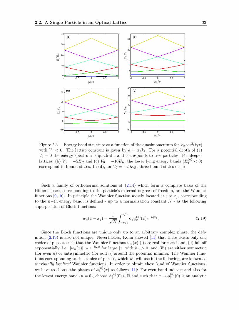
2.2. A Single Particle in an Optical Lattice 33
Figure 2.3. Energy band structure as a function of the quasimomentum for V0 cos2(klx)with V0 < 0. The lattice constant is given by a = π/kl. For a potential depth of (a)V0 = 0 the energy spectrum is quadratic and corresponds to free particles. For deeper
lattices, (b) V0 = −5ER and (c) V0 = −10ER, the lower lying energy bands (E(n)q < 0)
correspond to bound states. In (d), for V0 = −20ER, three bound states occur.
Such a family of orthonormal solutions of (2.14) which form a complete basis of theHilbert space, corresponding to the particle’s external degrees of freedom, are the Wannierfunctions [9, 10]. In principle the Wannier function mostly located at site xj , correspondingto the n−th energy band, is defined - up to a normalization constant N - as the followingsuperposition of Bloch functions:
wn(x− xj) =1√N
∫ π/a
−π/adqφ(n)
q (x)e−iqxj . (2.19)
Since the Bloch functions are unique only up to an arbitrary complex phase, the defi-nition (2.19) is also not unique. Nevertheless, Kohn showed [11] that there exists only onechoice of phases, such that the Wannier functions wn(x) (i) are real for each band, (ii) fall offexponentially, i.e. |wn(x)| ∼ e−hnx for large |x| with hn > 0, and (iii) are either symmetric(for even n) or antisymmetric (for odd n) around the potential minima. The Wannier func-tions corresponding to this choice of phases, which we will use in the following, are known asmaximally localized Wannier functions. In order to obtain these kind of Wannier functions,
we have to choose the phases of φ(n)q (x) as follows [11]: For even band index n and also for
the lowest energy band (n = 0), choose φ(n)q (0) ∈ R and such that q 7→ φ
(n)q (0) is an analytic

34 Background: Cold Atoms in Optical Lattices
Figure 2.4. Probability distribution of the Bloch functions for the lowest band and zero
quasimomentum,∣
∣
∣φ
(0)0 (x)
∣
∣
∣
2for a lattice depth of V0 = 0 (dotted, black line), V0 = −5ER
(solid, red line), V0 = −10ER (dashed, green line) and V0 = −20ER (dashed-dotted,blue line). If the lattice is absent, the particles are free, which implies a homogeneousprobability distribution. The deeper the lattice gets, the more the wave function getslocalized in every lattice well.
function. This can be ensured by choosing an equal sign for all coefficients in the Fouriersum (2.17). Then wn(x − xj) are symmetric around xj and real. For odd n, on the other
hand, choosing φ(n)q (0) purely imaginary, and imposing the same smoothness condition on
the Bloch functions lead to real but antisymmetric Wannier functions.
Since we restrict our investigations to very cold atoms, we only have to deal with Wan-nier functions of the lowest energy band. Examples of this Wannier functions are plotted inFig. 2.5(a). Here we plotted w0(x) for V0 = −5ER and V0 = −10ER. The deeper potentialprovides better localized wavefunctions. In Fig. 2.5(b) we depict the asymptotic behavior ofthe n = 0 Wannier functions on a logarithmic scale and compare it with their approxima-tions by groundstate wavefunctions of harmonic oscillators (2.13). The deeper the potential,the better is this approximation. Nevertheless, log(|wn(x)|) decreases linearly, whereas theharmonic oscillator functions are Gaussians, and show a quadratic behavior on a logarithmicscale.
2.3 The Bose-Hubbard Model
Originally, the Bose-Hubbard model was used to study systems in condensed matter theory,like electrons in periodic crystalline structures. For instance, Fisher et al. [12] were the firstto investigate the phase diagram of the Bose-Hubbard Hamiltonian at temperature T = 0.The application of this model to cold atoms in optical lattices was firstly discussed by Jakschet al. [13], which envisioned a wide variety of promising applications of AMO physics in thephysics of condensed matter. Although this model is nowadays commonly used, we exhibit
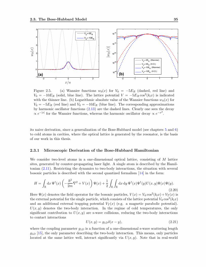
2.3. The Bose-Hubbard Model 35
(a) (b)
Figure 2.5. (a) Wannier functions w0(x) for V0 = −5ER (dashed, red line) andV0 = −10ER (solid, blue line). The lattice potential V = −5ER cos2(klx) is indicatedwith the thinner line. (b) Logarithmic absolute value of the Wannier functions w0(x) forV0 = −5ER (red line) and V0 = −10ER (blue line). The corresponding approximationsby harmonic oscillator functions (2.13) are the dashed lines. Clearly one sees the decay∝ e−|x| for the Wannier functions, whereas the harmonic oscillator decay ∝ e−x2
.
its naive derivation, since a generalization of the Bose-Hubbard model (see chapters 5 and 6)to cold atoms in cavities, where the optical lattice is generated by the resonator, is the basisof our work in this thesis.
2.3.1 Microscopic Derivation of the Bose-Hubbard Hamiltonian
We consider two-level atoms in a one-dimensional optical lattice, consisting of M latticesites, generated by counter-propagating laser light. A single atom is described by the Hamil-tonian (2.11). Restricting the dynamics to two-body interactions, the situation with severalbosonic particles is described with the second quantized formalism [14] in the form:
H =
∫
R
dx؆(x)
(
− ~2
2m∇2 + V (x)
)
Ψ(x) +1
2
∫
R
∫
R
dxdyΨ†(x)Ψ†(y)U(x, y)Ψ(x)Ψ(y).
(2.20)Here Ψ(x) denotes the field operator for the bosonic particles, V (x) = V0 cos2(klx)+VT (x) isthe external potential for the single particle, which consists of the lattice potential V0 cos2(klx)and an additional external trapping potential VT (x) (e.g. a magnetic parabolic potential).U(x, y) denotes the two-body interaction. In the regime of cold temperatures, the onlysignificant contribution to U(x, y) are s-wave collisions, reducing the two-body interactionsto contact interactions
U(x, y) = g1Dδ(x − y), (2.21)
where the coupling parameter g1D is a function of a one-dimensional s-wave scattering lengthg1D [15], the only parameter describing the two-body interaction. This means, only particleslocated at the same lattice well, interact significantly via U(x, y). Note that in real-world
36 Background: Cold Atoms in Optical Lattices
situations, the one-dimensional lattice is in principle only quasi one-dimensional, arising froma very tight confinement in the other two dimensions. In the 3D-case the contact interactionterm is modeled by a pseudopotential [16]
U(x) =4π~
2asm
δ3(x) = gδ3(x), (2.22)
where m is the mass of the atoms and as denotes the s-wave scattering length. The inte-gration in the second term of (2.20) has then to be performed over R
3 × R3. For tight axial
confinement, which is necessary in order to consider one-dimensional optical lattices (andtherefore the one-dimensional integration in the first term of (2.20)), the 3D-interaction canbe reduced to a one-dimensional coupling strength g1D [15].
In order to derive the Bose-Hubbard model, we expand the field operators in the Wannierbasis
Ψ(x) =
M∑
i=1
∞∑
n=0
wn(x− xi)bn,i, (2.23)
where bn,i is the bosonic annihilation operator for a particle in the energy band n, locatedat site i, i.e. trapped in the lattice well around the potential minimum at xi. As a firstapproximation we assume, such a low temperature T , that the corresponding energy is muchlower than the energy gap between the two lowest Bloch bands, approximately given by ~ωHO.In addition, we assume that this applies also for the mean interaction energies g1D〈ni〉, where〈ni〉 is the mean number of atoms at an arbitrary site i. If this is the case, we can restrictthe second sum in (2.23) to the lowest energy band n = 0,
Ψ(x) =M∑
i=1
w(x− xi)bi, (2.24)
where w(x) ≡ w0(x) and bi ≡ b0,i. Replacing the field operators in (2.20) by this expression,we obtain the following Hamiltonian:
H =∑
k,l
Eklb†kbl + V0
∑
k,l
Jklb†kbl +
∑
k,l
Vklb†kbl +
1
2
∑
i,j,k,l
Uijklb†ib
†jbkbl, (2.25)
where the first order matrix elements are given by
Ekl =
∫
R
dxw(x− xk)(
− ~2
2m∇2
)
w(x − xl), (2.26a)
Jkl =
∫
R
dxw(x− xk) cos2(kx)w(x− xl), (2.26b)
Vkl =
∫
R
dxw(x− xk)VT (x)w(x − xl). (2.26c)
The matrix elements for the on-site interaction reads as
Uijkl = g1D
∫
R
dxw(x− xi)w(x− xj)w(x− xk)w(x− xl). (2.27)

2.3. The Bose-Hubbard Model 37
The separation of the matrix elements for the kinetic energy (Ekl) and for the potentialenergy (JklV0) is artificial here and they can be simply added. If an optical cavity with anintracavity quantum field is present this is no longer true. Therefore we retain this separationhere.
Next, we assume that the variation of the additional external potential over the size of asingle lattice well is negligible, i.e. VT (x)w(x− xi) = VT (xi)w(x− xi). Therefore, due to theorthonormality of the Wannier functions, the contribution of the external potential amountsto a discretized energy shift
Vkl = VT (xk)
∫
R
dxw(x− xk)w(x− xl) = VT (xk)δkl = εkδkl. (2.28)
The on-site elements Jkk and Ekk are independent of the lattice site k, and are thereforedenoted by E0 and J0, respectively. The off-site elements Jk,lEkl for k 6= l are symmetric withrespect to the lattice sites, and describe tunneling to other wells. Here we can safely restrict tohopping between neighboring sites (this is known as the tight-binding approximation). Sincethe next-nearest elements are typically two orders of magnitude smaller than the nearest-neighbor term [see Fig. 2.6(a) and Fig. 2.6(b)] they can safely be neglected. This means,Ekl and Jkl with |k − l| > 1 are omitted, and we denote the neighboring tunneling elementsEl,l+1 and Jl,l+1 by E and J , respectively.
Figure 2.6. (a) Tunneling matrix elements for the kinetic energy for the nearestneighbors E/ER (red, solid line), where E ≡ E12, for the next-to-nearest neighborsE13/ER (blue, dashed line) and for the third neighbors E14/ER (black, dashed-dottedline) along one dimension as a function of the potential depth. (b) The same for thetunneling matrix element of the potential energy J ≡ J12 (red, solid line), J13 (blue,dashed line) and J14 (black, dashed-dotted line). The nearest neighbor elements are atleast two orders of magnitude larger and dominate.
Similar approximations can be performed for the on-site interaction matrix ele-ments (2.27). Here, only Uijkl with i = j = k = l have to be taken into account sincethe pure overlap integrals of Wannier functions with at least one Wannier function sited at a
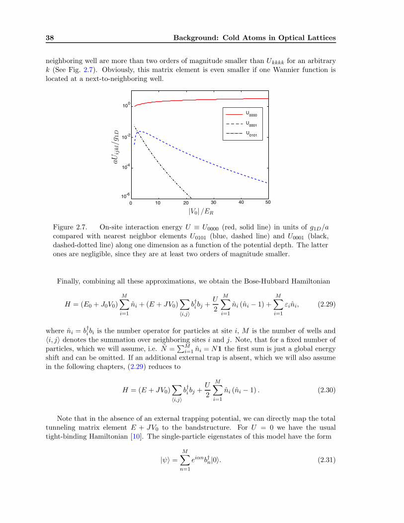
38 Background: Cold Atoms in Optical Lattices
neighboring well are more than two orders of magnitude smaller than Ukkkk for an arbitraryk (See Fig. 2.7). Obviously, this matrix element is even smaller if one Wannier function islocated at a next-to-neighboring well.
Figure 2.7. On-site interaction energy U ≡ U0000 (red, solid line) in units of g1D/acompared with nearest neighbor elements U0101 (blue, dashed line) and U0001 (black,dashed-dotted line) along one dimension as a function of the potential depth. The latterones are negligible, since they are at least two orders of magnitude smaller.
Finally, combining all these approximations, we obtain the Bose-Hubbard Hamiltonian
H = (E0 + J0V0)
M∑
i=1
ni + (E + JV0)∑
〈i,j〉b†i bj +
U
2
M∑
i=1
ni (ni − 1) +
M∑
i=1
εini, (2.29)
where ni = b†ibi is the number operator for particles at site i, M is the number of wells and〈i, j〉 denotes the summation over neighboring sites i and j. Note, that for a fixed number ofparticles, which we will assume, i.e. N =
∑Mi=1 ni = N1 the first sum is just a global energy
shift and can be omitted. If an additional external trap is absent, which we will also assumein the following chapters, (2.29) reduces to
H = (E + JV0)∑
〈i,j〉b†i bj +
U
2
M∑
i=1
ni (ni − 1) . (2.30)
Note that in the absence of an external trapping potential, we can directly map the totaltunneling matrix element E + JV0 to the bandstructure. For U = 0 we have the usualtight-binding Hamiltonian [10]. The single-particle eigenstates of this model have the form
|ψ〉 =
M∑
n=1
eiαnb†n|0〉. (2.31)
2.3. The Bose-Hubbard Model 39
The constant α is determined by periodic boundary conditions αl = 2πM , which we impose.Here l is an integer number. Applying the tight-binding Hamiltonian on |ψ〉 with eigenvalueEα brings us to the relation
2(E + JV0) = Eα. (2.32)
Obviously the total tunneling matrix element can then simply be found as
E + JV0 =max
(
E(0)q
)
−min(
E(0)q
)
4. (2.33)
The zero denotes the lowest energy band. The hopping matrix element can thus be easilycalculated from the Bloch band. Unfortunately this method does not work for the kineticenergy and the potential matrix element separately. Another approximation method is basedon the Mathieu functions, solving also the single-particle Hamiltonian (2.11). For deep enoughlattices, the matrix element is approximately given by [17]
E + JV0 =4√πER
( |V0|ER
)3/4
e−2√
|V0|/ER . (2.34)
The validity of this expression is shown in Fig. 2.8(f), where we compare the so estimated valueof the tunneling element with the exact one, derived with Wannier functions. Nevertheless,the same disadvantage as above comes here into play.
For deep lattices it is also possible to approximate the Wannier functions by groundstatewavefunctions of harmonic oscillators (2.13), which allows for analytic expressions of thematrix elements (2.26) and (2.27):
E0 =~
2
4mx20
, (2.35a)
E =~
2
4mx20
(
1− π2
2k2l x
20
)
e−π2/(4k2
lx20), (2.35b)
J0 =1 + e−k
2
lx20
2, (2.35c)
J =1− e−k2
lx20
2e−π
2/(4k2
lx20), (2.35d)
U =g1D√2πx0
. (2.35e)
Here x0 =√
~/(mωHO) = 1/k · (|V0| /ER)−1/4 is the width of the harmonic oscillator groundstate. In Fig. 2.8 we compare the various matrix elements, on-site and off-site, for kinetic andpotential energy as well as the on-site interaction U , calculated with the Wannier functionsand with the harmonic oscillator approximation, as a function of the relative potential depth|V0| /ER. The on-site elements from both methods are converging, which is not the case forthe off-site elements. Here, the harmonic oscillator elements always underestimate the realmatrix elements. The reason for this behavior is the much stronger decrease of the Gaussfunctions than of the Wannier functions [see Fig. 2.5(b)].
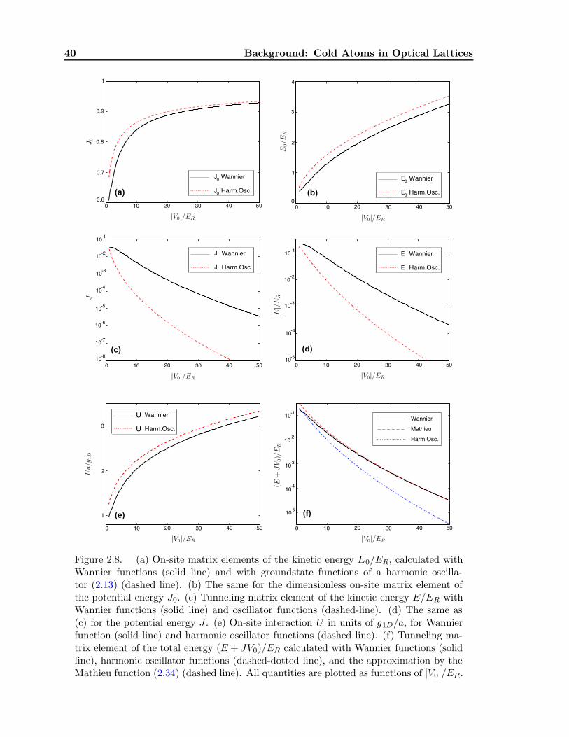
40 Background: Cold Atoms in Optical Lattices
Figure 2.8. (a) On-site matrix elements of the kinetic energy E0/ER, calculated withWannier functions (solid line) and with groundstate functions of a harmonic oscilla-tor (2.13) (dashed line). (b) The same for the dimensionless on-site matrix element ofthe potential energy J0. (c) Tunneling matrix element of the kinetic energy E/ER withWannier functions (solid line) and oscillator functions (dashed-line). (d) The same as(c) for the potential energy J . (e) On-site interaction U in units of g1D/a, for Wannierfunction (solid line) and harmonic oscillator functions (dashed line). (f) Tunneling ma-trix element of the total energy (E + JV0)/ER calculated with Wannier functions (solidline), harmonic oscillator functions (dashed-dotted line), and the approximation by theMathieu function (2.34) (dashed line). All quantities are plotted as functions of |V0|/ER.
2.3. The Bose-Hubbard Model 41
2.3.2 The Superfluid State and the Mott Insulator State
In the Hamiltonian (2.30) there is a competition between the tunneling matrix element E +JV0, which is essentially the kinetic energy element E, as we can see in Fig. 2.8(c) and(d), which tries to delocalize the particles and the interaction term U , which attempts tolocalize the particles and keeping the particle number fluctuations small. Essentially twoparameters characterize the system, the average particle density n = N/M and the ratiobetween interaction and hopping U/(E + JV0). Two main regimes exist for the system.On the one hand, the system can be either in a superfluid phase, where the single-particlewave functions are delocalized over the lattice. On the other hand, the system can be inthe Mott insulator phase, where the particles are localized on single lattice sites. One of thefirst investigations in this direction was the study of the phase diagram of the Bose-Hubbardmodel by Fisher et al. [12], which we schematically depict in Fig. 2.9. At that time, however,an experimental verification seemed far out of reach. One of the main advantages of therealization of the Bose-Hubbard model with cold atoms in optical lattices, is the tunabilityof the ratio U/(E + JV0) via the power of the lattice lasers. A lot of investigation on thissubject has now been done and also the first experimental realization of the Mott-insulatorto superfluid phase transition in the seminal work by Greiner et al. [18] has been performed.For a review of the current status of the research on the field see [7].
Let us first consider the regime, where the kinetic energy dominates over the on-siteinteraction, i.e. U/(E+JV0)→ 0. In this limit the ground state of the system is a superfluidstate, which in the case of a lattice with M sites and N particles can be written as
|SF〉 =1√N !
(
1
M
M∑
i=1
b†i
)N
|0〉, (2.36)
where |0〉 = |0, . . . , 0〉 denotes the state of an empty lattice. In this state all atoms occupythe same single-particle wavefunction, which is delocalized over the lattice. This macroscopicoccupation of one state realizes a Bose-Einstein condensate (BEC). Particle number fluctu-ations in a site i, (∆ni)
2 = 〈n2i 〉 − 〈ni〉2 are large and scale as the average density N/M .
Furthermore, the systems shows long-range off-diagonal coherence.
As U/(E + JV0) and hence the interaction energy increases, the particles repel eachother more and more. This impedes the tunneling of particles to a neighboring site, sincethe necessary kinetic energy for this process is insufficient to negotiate the repulsion energy.When the particle density n is equal to one, the ground state of the systems, consists ofa single localized particle in every well. Generally, a necessary condition for such a Mottinsulator state, is an integer mean particle density. For (E + JV0)/U → 0 the ground stateof the system is the Mott insulator state
|MI〉 =M∏
i=1
|n〉i (2.37)
for n = N/M ∈ N. This state has no particle number fluctuations and the off-diagonalcoherences decay exponentially with the distance of the respective sites.
In Fig. 2.9 we show this in the schematic picture of the Bose-Hubbard phase diagram, inthe grand canonical ensemble for fixed mean number of particles n = 〈N〉/M via a chemical
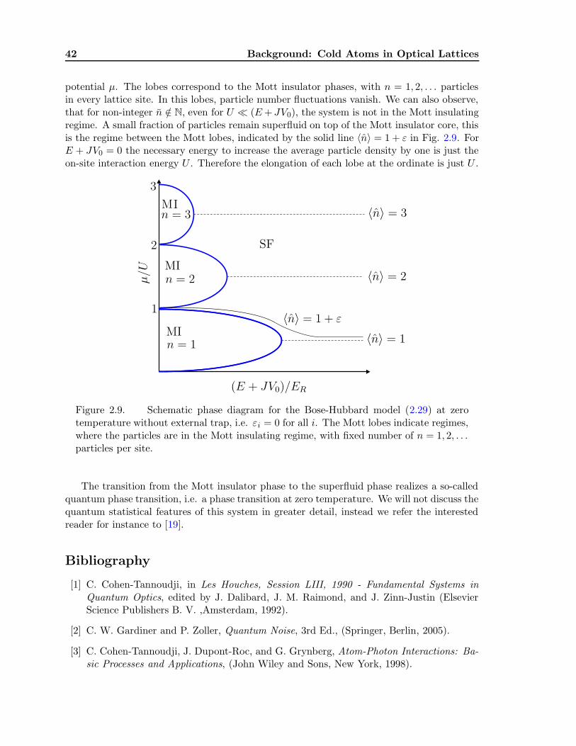
42 Background: Cold Atoms in Optical Lattices
potential µ. The lobes correspond to the Mott insulator phases, with n = 1, 2, . . . particlesin every lattice site. In this lobes, particle number fluctuations vanish. We can also observe,that for non-integer n /∈ N, even for U (E+JV0), the system is not in the Mott insulatingregime. A small fraction of particles remain superfluid on top of the Mott insulator core, thisis the regime between the Mott lobes, indicated by the solid line 〈n〉 = 1 + ε in Fig. 2.9. ForE + JV0 = 0 the necessary energy to increase the average particle density by one is just theon-site interaction energy U . Therefore the elongation of each lobe at the ordinate is just U .
Figure 2.9. Schematic phase diagram for the Bose-Hubbard model (2.29) at zerotemperature without external trap, i.e. εi = 0 for all i. The Mott lobes indicate regimes,where the particles are in the Mott insulating regime, with fixed number of n = 1, 2, . . .particles per site.
The transition from the Mott insulator phase to the superfluid phase realizes a so-calledquantum phase transition, i.e. a phase transition at zero temperature. We will not discuss thequantum statistical features of this system in greater detail, instead we refer the interestedreader for instance to [19].
Bibliography
[1] C. Cohen-Tannoudji, in Les Houches, Session LIII, 1990 - Fundamental Systems inQuantum Optics, edited by J. Dalibard, J. M. Raimond, and J. Zinn-Justin (ElsevierScience Publishers B. V. ,Amsterdam, 1992).
[2] C. W. Gardiner and P. Zoller, Quantum Noise, 3rd Ed., (Springer, Berlin, 2005).
[3] C. Cohen-Tannoudji, J. Dupont-Roc, and G. Grynberg, Atom-Photon Interactions: Ba-sic Processes and Applications, (John Wiley and Sons, New York, 1998).
BIBLIOGRAPHY 43
[4] P. S. Jessen and I. H. Deutsch, Optical Lattices, Adv. At. Mol. Opt. Phys. 37, 95 (1996).
[5] P. B. Blakie and C. W. Clark, Wannier States and Bose-Hubbard Parameters for 2DOptical Lattices, J. Phys. B 37, 1391 (2004).
[6] D. Jaksch and P. Zoller, The Cold Atom Hubbard Toolbox, Ann. Phys. 315, 52 (2005).
[7] M. Lewenstein, A. Sanpera, V. Ahufinger, B. Damski, A. Sen De, and U. Sen, UltracoldAtomic Gases in Optical Lattices: Mimicking Condensed Matter Physics and Beyond,Adv. Phys. 56, 243 (2007).
[8] M. Abramovitz and I. A. Stegun, Handbook of Mathematical Functions with Formulas,Graphs, and Mathematical Table, (Dover, 1972).
[9] N. W. Ashcroft and N. D. Mermin, Solid State Physics, International Ed., (Holt Rinehartand Winston, 1987).
[10] C. Kittel, Introduction to Solid State Physics, 8th Ed., (John Wiley and Sons, New York,2004).
[11] W. Kohn, Analytic Properties of Bloch Waves and Wannier Functions, Phys. Rev. 115,809 (1959).
[12] M. P. A. Fisher, P. B. Weichmann, G. Grinstein, and D. S. Fisher, Boson Localizationand the Superfluid-Insulator Transition, Phys. Rev. B 40, 546 (1989).
[13] D. Jaksch, C. Bruder, J. I. Cirac, C. W. Gardiner, and P. Zoller, Cold Bosonic Atomsin Optical Lattices, Phys. Rev. Lett. 81, 3108 (1998).
[14] See, for example, A. Galindo and P. Pascual, Quantum Mechanics II, (Springer, Berlin,1990).
[15] M. Olshanii, Atomic Scattering in the Presence of an External Confinement and a Gasof Impenetrable Bosons, Phys. Rev. Lett. 81, 938 (1998).
[16] See, for example, K. Huang, Statistical Mechanics, (Wiley, New York 1987).
[17] W. Zwerger,Mott-Hubbard Transition of Cold Atoms in Optical Lattices, J. Opt. B 5, 9(2003).
[18] M Greiner, O. Mandel, T. W. H’ansch, and IBloch, Quantum Phase Transition from aSuperfluid to a Mott Insulator in a Gas of Ultracold Atoms, Nature (London), 415, 39(2002).
[19] S. Sachdev, Quantum Phase Transitions, (Cambridge University Press, 1999).

Chapter 3
Background: Basics of Cavity Quantum
Electrodynamics (CQED)
In chapter 2 we briefly reviewed some of the main features of the theory of cold atoms inoptical lattices and discussed the physical applications thereof, allowing for an experimentalrealization of the Mott insulator to superfluid phase transition.
In this chapter we will deal with another versatile quantum optical system. Opticalcavities turned out to be a useful tool to significantly enhance the interaction between matterand light on a fundamental quantum level, providing for a variety of applications in AMOphysics. Moreover, in the strong coupling regime, a backaction mechanism of the intracavitylight field on the motion of atoms inside the resonator and vice versa exists. Hence, atomand cavity has to be considered as a single entity, the atom-cavity system. A number ofimpressive results based on this complex interaction has been predicted and experimentallyverified in the last years.
In this chapter on basic essentials of cavity QED, we first present some general propertiesof cavities, followed by a discussion of the Jaynes-Cummings Hamiltonian [1], describing theinteraction of an atom with a single mode of the cavity. Next we introduce dissipation, namelyspontaneous emission of photons from atoms and loss of cavity photons to the system, whichis now also coherently driven. Then we discuss how to eliminate the excited state of thetwo-level atom from the dynamics, to obtain an effective Hamiltonian, which is the crucialelement in the description of the resonator-generated optical lattice, as a generalization of theoptical lattices, discussed in the previous chapter. Furthermore, we briefly show how to addan additional far-detuned dipole trap (classical optical lattice), not influenced by the cavitymode, as an additional, useful element of the model. Finally, we consider motion transverseto the cavity axis (up to here only motion along the cavity axis will be allowed), which leadsto a slight variation in the corresponding Hamiltonian.
3.1 Atoms in Optical Cavities
This section is devoted to recapitulate the important properties of optical cavity resonators.We start with a discussion about classical resonators, followed by introducing ideal (lossless)quantum cavities, i.e. atoms inside the resonator are coupled to the quantized intracavityfield. Finally we add dissipation to the system, in order to describe more realistic situations.
3.1.1 Optical Cavities
We consider a Fabry-Perot resonator, consisting of two highly reflective mirrors, wheremonochromatic light is coupled in at one mirror, and the transmitted intensity is measured

46 Background: Basics of Cavity Quantum Electrodynamics (CQED)
at the opposite mirror. In order to achieve a simple illustration, we assume the mirrorsto be flat and parallel with an axial distance of L (x−direction). An incident plane waveEin = E0 cos(kx) leaks into the empty cavity via one of the mirrors, as depicted in Fig. 3.1.
Figure 3.1. Schematic diagram of a Fabry-Perot type resonator, consisting of twoparallel mirrors with distance L. On the left mirror light is coupled in, on the rightmirror it leaks out of the resonator, where it is detected.
Generally, the normal modes of an empty cavity are defined as the solutions of theHelmholtz equation
(
∇2 +ω2
c2
)
u(x) = 0, (3.1)
which fulfill appropriate boundary conditions, corresponding to the specific mirror geometry.The electric field is a superposition of the eigenmodes unmk(x) with eigenfrequencies ωnmk.In our one-dimensional example this is fairly easy, since the electric field has to vanish at themirror, we obtain
un(x) = sin(πn
Lx)
and ωn =nπc
Lfor n ∈ N (3.2)
Two consecutive longitudinal modes of the resonator are characterized by consecutivemode numbers n, which are typically very large. The corresponding difference in frequencyis called free spectral range
νFSR ≡ωn+1 − ωn
2π=
c
2L(3.3)
The transmitted light has a maximum, when its frequency corresponds to one of theeigenfrequencies. Hence, two peaks in the transmission signal are separated by νFSR. If themirrors are not of this perfect (and idealistic) form, the mode functions are much more com-plicated and of course in reality three-dimensional. This implies the appearance of transversemodes, i.e. modes with transverse (here y− and z−direction) intensity dependence, like thetransverse-electro-magnetic modes TEMnm. In a cavity formed by two spherical mirrors, themost fundamental mode is the TEM00 mode [2]. This mode is also called Gaussian mode,since - near the cavity center - its radial dependence is that of a Gaussian function1
u00(x) = sin(kx)e−(y2+z2)/w20 , (3.4)
1In the rest of this thesis, though, we will use cos(kx) instead of the sin-function. This amounts just in anaddition of a global phase and makes physically no difference. With the cosine, we have a potential well atx = 0.

3.1. Atoms in Optical Cavities 47
where the beam radius w(x) = w0
√
1 + 4x2/(k2w40) at the cavity center (x = 0) is called
waist of the cavity and k = 2π/λ is the mode wavenumber. Here we omitted the longitudinalmode number, which precisely has to be taken into account via λ. For a symmetric cavitythe waist can be calculated [3]:
w20 =
L
k
√
2R − LL
. (3.5)
Here, R is the radius of curvature of the mirror. For a confocal cavity (R = L) this reducesto w2
0 = L/k. The mode volume of the cavity is the integral of the squared modulus of thecorresponding mode function, i.e.
V =
∫
R3
d3x |u00(x)|2 ≈ πw20
4L, (3.6)
if we assume that the edges of the cavity mirrors at x = 0 and x = L are impenetrable,resulting in a vanishing mode function for x < 0 and x > L.
Let us now come back to our simplified plane mirror model and assume, that both mirrorshave a reflectivity R, a transmittivity T and a loss rate L, resulting from absorption andscattering in the mirror medium. Furthermore we assume, that the cavity is enclosed by avacuum, i.e. the index of refraction is one. At any of the two mirrors the relationR+T +L = 1must hold. According to Airy’s formula, the total transmittivity of the resonator is [4]
Tcav =T 2
(1−R)2 + 4R sin2(kL)(3.7)
Figure 3.2. Transmittivity of the Fabry-Perot resonator corresponding to (3.7) as afunction of the frequency of the incoming light. The distance between the peaks of theLorentzians is called the free spectral range νFSR. The linewidth (FWHM) δν definesthe cavity decay rate κ.
When the frequency of the incoming field is on resonance with one of the longitudinalmodes (kL = 2πn), this expression presumes its maximum Tmax = T 2/(1 −R)2. Expanding

48 Background: Basics of Cavity Quantum Electrodynamics (CQED)
the sin−function in the denominator of (3.7), which is possible for wavenumbers k = ω/cclose to one of the mode frequencies, we obtain a Lorentz profile for (3.7) around the peakat ν = nνFSR (see Fig. 3.2)
Tcav ≈Tmax
1 + 4(
FνFSR
)2(∆ν)2
, (3.8)
where ∆ν = ν − nνFSR. Here we defined a very important characteristic parameter forresonators, the finesse F by
F =π√R
1−R . (3.9)
Note, that the finesse solely depends on the reflectivity of the mirror and gives a measure forthe resolutions of the light field in the resonator, before it leaks out of the cavity. From thisLorentzian we can easily read off the width (FWHM) δν = κ/π (κ is therefore known as thecavity loss rate)
δν =κ
π=νFSR
F . (3.10)
Finally the quality factor, or Q-factor, of a resonator at resonance is defined as 2π times theratio of stored energy in the cavity to energy loss per oscillation period, i.e.
Q = 2πW
∆W= ω
W
PL, (3.11)
where W is the energy, stored in the resonator, ∆W = τPL the energy loss per oscillationperiod (duration τ) and PL = −dW
dt the energy loss per unit time. Using the decay constantof the resonator, κ = PL/W , we obtain:
Q =ω
κ= 2πn
νFSR
κ= 2nF . (3.12)
Here, n denotes the number of the longitudinal mode.
We conclude this section with an overview of current state-of-the-art numbers, whichexperimental cavity QED groups have achieved. The group of Jeff Kimble at Caltech [5]use a cavity with a length of L = 42.2µm, waist w0 = 20µm and mirrors with a curvatureradius of R = 20cm. The finesse has a value of F = 4.2 × 10⁵ and at a cavity frequency ofω = 2.211MHz (corresponding to the D2 line of atomic Caesium λ = 852.4nm) a Q-factor ofQ = 8.584× 10⁷. In one of the most recent experiments in Gerhard Rempe’s group at MPQGarching [6] the cavity in use has a length of L = 0.122mm and a waist of w0 = 29µm. Theyoperate at a frequency of ω = 2.416MHz, corresponding to λ = 780.2nm. The finesse of thecavity is F = 4.4× 10⁵ and its quality factor Q = 1.282 × 10⁸.
3.1.2 The Jaynes-Cummings Hamiltonian
We consider here a single two-level atom, interacting with a single mode of the quantizedelectromagnetic field, first investigated by Jaynes [1]. This model is a reasonable approxi-mation for an atom interacting with the field inside an optical resonator without losses. In

3.1. Atoms in Optical Cavities 49
principle, the procedure is similar to the case of the interaction with a classical field, pre-sented in Sec. 2.1.1. A single one-dimensional standing wave quantized mode with frequencyωc is given by [7]
E(x) = i
√
~ωc2ε0V
u(x)aε + h.c. (3.13)
Here V denotes the quantization volume and u(x) the mode function of the cavity mode (3.6).The annihilation operator of a photon of the considered mode is given by a ≡ a, whereas a†
corresponds to the creation of a cavity photon. Near the center of a confocal, Fabry-Perotcavity the mode function in axial direction (here: x−direction) is cosine-like, whereas intransverse direction, the mode function decays as a Gaussian,
u(x) = cos(kx)e−(y2+z2)/w20 . (3.14)
In the following, we will neglect the transversal dependence and assume the region of inter-action is exactly in the center of the cavity. We assume the ground state energy of the atomto be zero (Eg = 0), and use the electromagnetic dipole and long-wavelength approximation.Then the Hamiltonian for a single atom, interacting with a single quantized mode is given by
H = HA +HF +HI (3.15)
=p2
2m+ ~ωeg|e〉〈e| + ~ωc
(
a†a+1
2
)
− i~g(x)(
a− a†)
⊗ (σ+ + σ−) ,
where g(x) = 〈e|d·ε|g〉 cos(kx)√
ωc/(2ε0V ~) denotes the coupling strength. The other no-tations are the same as in Sec. 2.1.1. Again the interaction Hamiltonian HI consists of tworesonant terms σ+ ⊗ a, σ− ⊗ a†, and two non-resonant terms σ+ ⊗ a†, σ− ⊗ a. The firstcorrespond to a transition of the atom |g〉 → |e〉 accompanied by the annihilation of a photonof the field mode and a transition |e〉 → |g〉, together with the creation of a photon, bothof these processes are energy conserving. The latter ones correspond to a transition of theatom |g〉 → |e〉 accompanied by the emission of a photon of the field mode and a transition|e〉 → |g〉, together with the annihilation of a photon. They are highly off-resonant and donot conserve energy. Therefore we can safely neglect them (rotating wave approximation).Finally the Hamiltonian, after a simple energy shift reads as follows:
H =p2
2m+ ~ωeg|e〉〈e| + ~ωca
†a− i~g(x)(
σ+a− σ−a†)
. (3.16)
This is the well known Jaynes-Cummings Hamiltonian. From this point on we omit thetensor product between operators acting on different Hilbert spaces. Let us briefly reviewthe properties of this system, which can easily be solved analytically. If we neglect, for themoment, the translational degrees of freedom, the ground state of this system is |g, 0〉, wherethe atom is in its internal ground state and zero photons are present in the cavity. Generallythe eigenstates are superpositions of n+ 1 photons in the cavity and the atom in the groundstate, |g, n + 1〉, and n photons in the cavity, but the atom in the excited state, |e, n〉. Weformulate this as follows:
|+, n〉 = cos θn|e, n〉 + sin θn|g, n+ 1〉, (3.17a)
|−, n〉 =− sin θn|e, n〉+ cos θn|g, n+ 1〉. (3.17b)
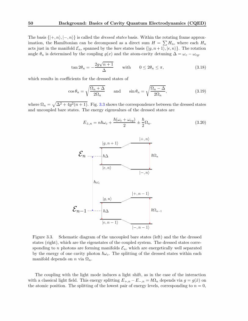
50 Background: Basics of Cavity Quantum Electrodynamics (CQED)
The basis |+, n〉, |−, n〉 is called the dressed states basis. Within the rotating frame approx-imation, the Hamiltonian can be decomposed as a direct sum H =
∑
Hn, where each Hn
acts just in the manifold En, spanned by the bare states basis |g, n+1〉, |e, n〉. The rotationangle θn is determined by the coupling g(x) and the atom-cavity detuning ∆ = ωc − ωeg.
tan 2θn = −2g√n+ 1
∆with 0 ≤ 2θn ≤ π, (3.18)
which results in coefficients for the dressed states of
cos θn =
√
Ωn + ∆
2Ωnand sin θn =
√
Ωn −∆
2Ωn, (3.19)
where Ωn =√
∆2 + 4g2(n+ 1). Fig. 3.3 shows the correspondence between the dressed statesand uncoupled bare states. The energy eigenvalues of the dressed states are
E±,n = n~ωc +~(ωc + ωeg)
2± ~
2Ωn. (3.20)
Figure 3.3. Schematic diagram of the uncoupled bare states (left) and the the dressedstates (right), which are the eigenstates of the coupled system. The dressed states corre-sponding to n photons are forming manifolds En, which are energetically well separatedby the energy of one cavity photon ~ωc. The splitting of the dressed states within eachmanifold depends on n via Ωn.
The coupling with the light mode induces a light shift, as in the case of the interactionwith a classical light field. This energy splitting E+,n−E−,n = ~Ωn depends via g = g(x) onthe atomic position. The splitting of the lowest pair of energy levels, corresponding to n = 0,

3.1. Atoms in Optical Cavities 51
is called normal mode splitting or vacuum Rabi-splitting. At resonance (∆ = 0) its value isjust given by the, spatial dependent, coupling strength g(x)
∆E0(x) = 2~g(x) (3.21)
This normal mode is visible, when the atom is strongly interacting with the a single pho-ton of the cavity, which implies that the coupling constant is larger than the correspondinglinewidths, i.e. g0 (γ, κ, τ−1), where τ is the interaction time of the atom and the cavitymode. g0 denotes the maximum of the coupling constant. Meeting these criteria experi-mentally is a very hard and complicated task, especially for cavities of optical frequencies.The first who observed the normal mode splitting in the optical regime were Thompson etal. [8]. The opposite limit κ g is called bad-cavity limit. Recent experimental numbersare, for instance, (g0, κ, γ)/2π = (34, 4.1, 2.5) MHz in Kimble’s group [5], while at the MPQin Garching the group of Rempe applies (g0, κ, γ)/2π = (16, 1.4, 3) MHz in the blue-detuneddipole trap experiment [6].
For a not too large coupling constant, we can calculate approximate energy shifts of theeigenstates of (3.16), using time-independent perturbation theory.
∆E ≈− ~g2(x)n+ 1
∆for |g, n+ 1〉, (3.22a)
∆E ≈+ ~g2(x)n+ 1
∆for |e, n〉. (3.22b)
Therefore we are in a similar situation as in the classical model before (2.7), with thedifference, that the depth of the cavity-induced lattice now depends on the number of photonsin the cavity mode. In Figure 3.4 we schematically depict the dependence of the energyspectrum on the axial position of the atom, within one well. Since the energy is increasingwith n this energy spectrum is known as the Jaynes-Cummings ladder. Since dissipativeeffects play a crucial role in cavities, we postpone a more detailed discussion of the resonator-generated lattice, after an introduction of lossy channels and coherent driving schemes to thecavity. Note that here at least one photon has to be present to realize this potential. Thestate |g, 0〉 experiences no energy shift. Other models exist, where also an empty cavity caninduce trapping potentials [9].
3.1.3 Open Systems - Dissipation
The Jaynes-Cummings Hamiltonian, derived in the previous section, describes closed systemsand therefore does not take into account any losses whatsoever. This simplification is in mostexperimental situations too crude and interactions of the system with the environment cannotbe ignored. From the various possible loss channels, only two are of major importance for ourstudies. Our system is assumed to be coupled to the environment via spontaneous emission ofphotons from the atoms and via loss of photons from the cavity. Not only that these dampingmechanisms allow to gain information about the system, i.e. the atoms and the intracavityfield, they also provide the necessary channel to transport entropy out of the system, a basicrequirement to perform cavity cooling.
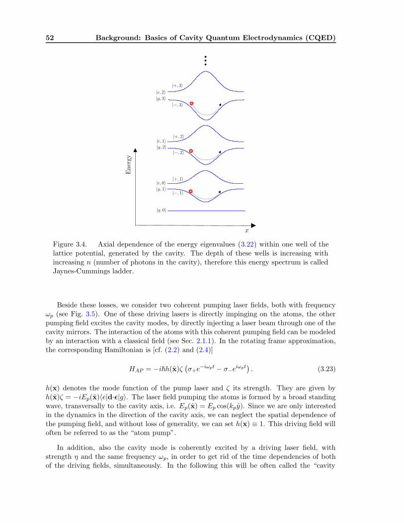
52 Background: Basics of Cavity Quantum Electrodynamics (CQED)
Figure 3.4. Axial dependence of the energy eigenvalues (3.22) within one well of thelattice potential, generated by the cavity. The depth of these wells is increasing withincreasing n (number of photons in the cavity), therefore this energy spectrum is calledJaynes-Cummings ladder.
Beside these losses, we consider two coherent pumping laser fields, both with frequencyωp (see Fig. 3.5). One of these driving lasers is directly impinging on the atoms, the otherpumping field excites the cavity modes, by directly injecting a laser beam through one of thecavity mirrors. The interaction of the atoms with this coherent pumping field can be modeledby an interaction with a classical field (see Sec. 2.1.1). In the rotating frame approximation,the corresponding Hamiltonian is [cf. (2.2) and (2.4)]
HAP = −i~h(x)ζ(
σ+e−iωpt − σ−eiωpt
)
. (3.23)
h(x) denotes the mode function of the pump laser and ζ its strength. They are given byh(x)ζ = −iEp(x)〈e|d·ε|g〉. The laser field pumping the atoms is formed by a broad standingwave, transversally to the cavity axis, i.e. Ep(x) = Ep cos(kpy). Since we are only interestedin the dynamics in the direction of the cavity axis, we can neglect the spatial dependence ofthe pumping field, and without loss of generality, we can set h(x) ≡ 1. This driving field willoften be referred to as the “atom pump”.
In addition, also the cavity mode is coherently excited by a driving laser field, withstrength η and the same frequency ωp, in order to get rid of the time dependencies of bothof the driving fields, simultaneously. In the following this will be often called the “cavity

3.1. Atoms in Optical Cavities 53
Figure 3.5. Scheme of atoms in a cavity, interacting with a single cavity mode.The system is coupled to a reservoir via cavity loss, characterized by the loss rate κand spontaneous emission from photons, described by the spontaneous emission rate γ.Furthermore, two pump lasers, both with the same frequency ωp but different strength,are coherently driving the system.
pump”. The Hamiltonian, describing this contribution is
HCP = −i~η(
aeiωpt − a†e−iωpt)
. (3.24)
Although, in principle, η and ζ can be chosen complex, to describe other relative phases, whichalso allows for interesting effects [10], we restrict in this work on real η and ζ. Altogether,the Hamiltonian describing the non-dissipative evolution of the system thus is
HS = HA +HF +HI +HAP +HCP (3.25)
=p2
2m+ ~ωeg|e〉〈e| + ~ωca
†a− i~g(x)(
σ+a− σ−a†)
−i~ζ(
σ+e−iωpt − σ−eiωpt
)
− i~η(
aeiωpt − a†e−iωpt)
.
To eliminate the time dependence, we perform a unitary transformation |ψ〉 = U(t)|ψ〉, whereU = exp[iωpt(σ+σ−+a†a)]. This corresponds to a transformation H = UHU † + i~
(
ddtU
)
U †.Omitting the tilde we obtain
HS =p2
2m− ~∆a|e〉〈e| − ~∆ca
†a− i~g(x)(
σ+a− σ−a†)
− i~ζ (σ+ − σ−)− i~η(
a− a†)
,
(3.26)
where ∆a = ωp−ωeg and ∆c = ωp−ωc denote the atom-pump detuning and the cavity-pumpdetuning, respectively.
In order to develop a theoretical description for the interaction of a system S with areservoir R, which form altogether a Hilbert space H = HS ⊗ HR. The system is then
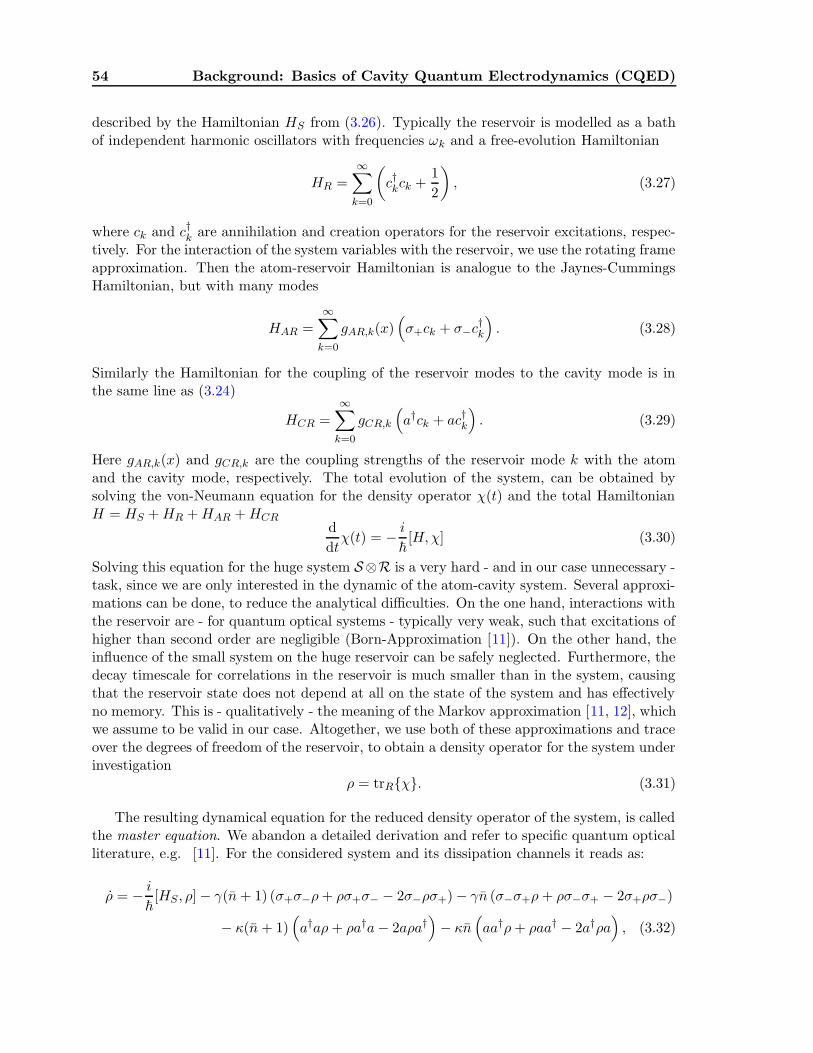
54 Background: Basics of Cavity Quantum Electrodynamics (CQED)
described by the Hamiltonian HS from (3.26). Typically the reservoir is modelled as a bathof independent harmonic oscillators with frequencies ωk and a free-evolution Hamiltonian
HR =∞∑
k=0
(
c†kck +1
2
)
, (3.27)
where ck and c†k are annihilation and creation operators for the reservoir excitations, respec-tively. For the interaction of the system variables with the reservoir, we use the rotating frameapproximation. Then the atom-reservoir Hamiltonian is analogue to the Jaynes-CummingsHamiltonian, but with many modes
HAR =
∞∑
k=0
gAR,k(x)(
σ+ck + σ−c†k
)
. (3.28)
Similarly the Hamiltonian for the coupling of the reservoir modes to the cavity mode is inthe same line as (3.24)
HCR =
∞∑
k=0
gCR,k
(
a†ck + ac†k
)
. (3.29)
Here gAR,k(x) and gCR,k are the coupling strengths of the reservoir mode k with the atomand the cavity mode, respectively. The total evolution of the system, can be obtained bysolving the von-Neumann equation for the density operator χ(t) and the total HamiltonianH = HS +HR +HAR +HCR
d
dtχ(t) = − i
~[H,χ] (3.30)
Solving this equation for the huge system S⊗R is a very hard - and in our case unnecessary -task, since we are only interested in the dynamic of the atom-cavity system. Several approxi-mations can be done, to reduce the analytical difficulties. On the one hand, interactions withthe reservoir are - for quantum optical systems - typically very weak, such that excitations ofhigher than second order are negligible (Born-Approximation [11]). On the other hand, theinfluence of the small system on the huge reservoir can be safely neglected. Furthermore, thedecay timescale for correlations in the reservoir is much smaller than in the system, causingthat the reservoir state does not depend at all on the state of the system and has effectivelyno memory. This is - qualitatively - the meaning of the Markov approximation [11, 12], whichwe assume to be valid in our case. Altogether, we use both of these approximations and traceover the degrees of freedom of the reservoir, to obtain a density operator for the system underinvestigation
ρ = trRχ. (3.31)
The resulting dynamical equation for the reduced density operator of the system, is calledthe master equation. We abandon a detailed derivation and refer to specific quantum opticalliterature, e.g. [11]. For the considered system and its dissipation channels it reads as:
ρ = − i~[HS , ρ]− γ(n+ 1) (σ+σ−ρ+ ρσ+σ− − 2σ−ρσ+)− γn (σ−σ+ρ+ ρσ−σ+ − 2σ+ρσ−)
− κ(n+ 1)(
a†aρ+ ρa†a− 2aρa†)
− κn(
aa†ρ+ ρaa† − 2a†ρa)
, (3.32)
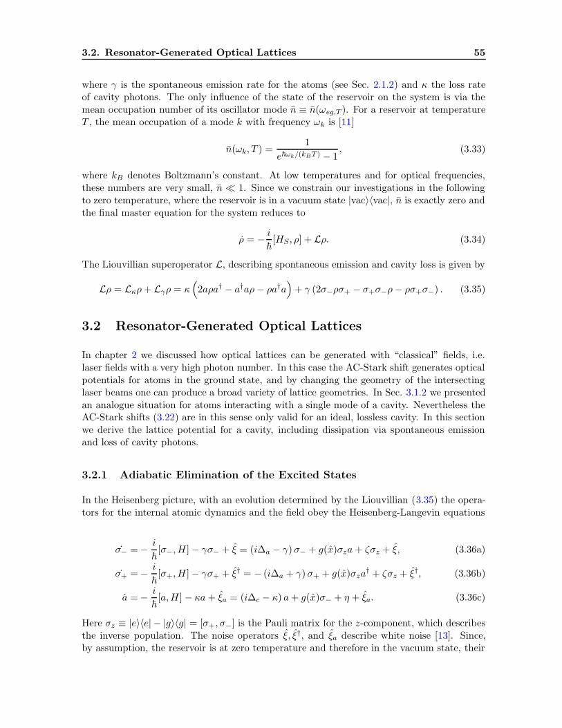
3.2. Resonator-Generated Optical Lattices 55
where γ is the spontaneous emission rate for the atoms (see Sec. 2.1.2) and κ the loss rateof cavity photons. The only influence of the state of the reservoir on the system is via themean occupation number of its oscillator mode n ≡ n(ωeg,T ). For a reservoir at temperatureT , the mean occupation of a mode k with frequency ωk is [11]
n(ωk, T ) =1
e~ωk/(kBT ) − 1, (3.33)
where kB denotes Boltzmann’s constant. At low temperatures and for optical frequencies,these numbers are very small, n 1. Since we constrain our investigations in the followingto zero temperature, where the reservoir is in a vacuum state |vac〉〈vac|, n is exactly zero andthe final master equation for the system reduces to
ρ = − i~[HS , ρ] + Lρ. (3.34)
The Liouvillian superoperator L, describing spontaneous emission and cavity loss is given by
Lρ = Lκρ+ Lγρ = κ(
2aρa† − a†aρ− ρa†a)
+ γ (2σ−ρσ+ − σ+σ−ρ− ρσ+σ−) . (3.35)
3.2 Resonator-Generated Optical Lattices
In chapter 2 we discussed how optical lattices can be generated with “classical” fields, i.e.laser fields with a very high photon number. In this case the AC-Stark shift generates opticalpotentials for atoms in the ground state, and by changing the geometry of the intersectinglaser beams one can produce a broad variety of lattice geometries. In Sec. 3.1.2 we presentedan analogue situation for atoms interacting with a single mode of a cavity. Nevertheless theAC-Stark shifts (3.22) are in this sense only valid for an ideal, lossless cavity. In this sectionwe derive the lattice potential for a cavity, including dissipation via spontaneous emissionand loss of cavity photons.
3.2.1 Adiabatic Elimination of the Excited States
In the Heisenberg picture, with an evolution determined by the Liouvillian (3.35) the opera-tors for the internal atomic dynamics and the field obey the Heisenberg-Langevin equations
σ− =− i
~[σ−,H]− γσ− + ξ = (i∆a − γ) σ− + g(x)σza+ ζσz + ξ, (3.36a)
σ+ =− i
~[σ+,H]− γσ+ + ξ† = − (i∆a + γ) σ+ + g(x)σza
† + ζσz + ξ†, (3.36b)
a =− i
~[a,H] − κa+ ξa = (i∆c − κ) a+ g(x)σ− + η + ξa. (3.36c)
Here σz ≡ |e〉〈e| − |g〉〈g| = [σ+, σ−] is the Pauli matrix for the z-component, which describesthe inverse population. The noise operators ξ, ξ†, and ξa describe white noise [13]. Since,by assumption, the reservoir is at zero temperature and therefore in the vacuum state, their

56 Background: Basics of Cavity Quantum Electrodynamics (CQED)
expectation values vanish and we can neglect these noise terms. The mode function corre-sponds to a standing wave, Fabry-Perot cavity, i.e. g(x) = g0 cos(kx). When the cavity isonly very weakly driven, the systems Hilbert space consists of the states |g, 1〉 or |e, 0〉, andcontributions of other states can be neglected [14]. Hence,
〈aσz〉 = −〈a〉. (3.37)
Nevertheless, in situations where the excited state is very weakly populated, this relationholds at least approximately. This is the so-called low-saturation regime, where the saturationparameter s = g2
0/(∆2a + γ2) (see also Sec. 2.1.1) is very small, s 1. This is a regime where
typical quantum optical situations take place, and rather easily attainable, by choosing alarge atom-pump detuning ∆a. More generally, this method consists of replacing σz by itsexpectation value 〈σz〉, a technique called bosonisation [15], since the commutation relationsfor Pauli matrices are modified to bosonic commutation relations: [σ−, σ+] = −σz → −〈σz〉.Then the equations (3.36) become linear, and 〈σz〉, which is also called population inversionhas only the role as a parameter, which has to be chosen self-consistently. Nevertheless, forlow saturation, the population inversion can be well approximated by -1. In this regime thetimescale of the ground state evolution is much longer than those of the excited state. Hence,we can set the derivatives in in (3.36a) and (3.36b) to zero, as well as σz = −1. Then theexcited state is adiabatically eliminated from the dynamics. The steady state values of theoperators σ± follow then self-explanatory
σ− = −ζ + g(x)a
γ − i∆aand σ+ = −ζ + g(x)a†
γ + i∆a. (3.38)
After deriving these steady state “values” of these operators, we can proceed along twodifferent lines. On the one hand, we can replace them in the equation for the field (3.36c),yielding
a =[
i∆c − κ− (Γ0 + iU0) cos2(kx)]
a+ η − (γeff + iηeff) cos(kx), (3.39)
where we applied the specific form of the mode function g(x) = g0 cos(kx) and introducedthe following abbreviations, characterizing the atom’s dispersive and absorptive influence onthe cavity field:
U0 =g20∆a
γ2 + ∆2a
and Γ0 =g20γ
γ2 + ∆2a
. (3.40)
Here U0 can be interpreted as the energy light shift per photon for the atom, which willbe clarified with equation (3.42) and Γ0 as the photon loss probability per atom throughincoherent scattering. The other two terms are only relevant in the case, where the atomsare directly pumped and therefore reflect the influence of the atomic position on the field.
γeff =g0ζγ
γ2 + ∆2a
and ηeff =g0ζ∆a
γ2 + ∆2a
. (3.41)
On the other hand, we can also replace σ± by their steady state expressions (3.38) in theHamiltonian (3.26) and in the spontaneous emission part of the Liouvillian (3.35). In this

3.2. Resonator-Generated Optical Lattices 57
way we obtain an effective Hamiltonian (choosing normal order for the field operators), whichthen solely depends on the atom’s external degrees of freedom and the cavity field. Thus,
Heff =p2
2m+ ~U0 cos2(kx)a†a+ ~ηeff cos(kx)
(
a+ a†)
− i~η(
a− a†)
. (3.42)
Now the interpretation of U0 is clear. This is the analogue of the classical AC-Stark lightshift (2.10), per one photon (〈a†a〉 = 1). The terms corresponding to Γ0 and γeff arise fromthe replacement in the Liouvillian Lγ , which reads as
Lγ,eff = Γ0 cos2(kx)(
2aρa† − a†aρ− ρa†a)
+ γeff
[
a− a†, ρ]
. (3.43)
This method must - of course - lead also to the same dynamical equation as (3.39) for thefield. This is easy to check by calculating
d
dt〈a〉 = trρa with ρ = − i
~[Heff, ρ] + Lκρ+ Lγ,effρ. (3.44)
A major part of our work is the derivation of a generalized Bose-Hubbard model, whichincludes also resonator-generated optical lattices and the cavity as a dynamical element.This procedure requires a many-particle Hamiltonian in second quantization formalism (seeSec. 2.3.1). The implementation of (3.42) as the corresponding single-particle Hamiltonianprovides a generalized Hamiltonian with adiabatically eliminated excited states. Nevertheless,it is also possible to use (3.26) as a single-particle Hamiltonian in the second quantizationformalism and then eliminate the excited state of the atoms. This leads finally to the sameBose-Hubbard Hamiltonian (see chapter 6).
Finally we can make a useful approximation. In the rest of this thesis, we work in aregime far off resonance, i.e. ∆a γ. Hence U0 Γ0 and ηeff γeff. This allows us toneglect spontaneous emission at all and set γ = 0 in the equations above.
3.2.2 Intracavity trapping potential
The trapping depth of the resonator-generated optical lattice depends on two quantities, thecoupling strength U0 and the number of photons in the cavity field. In order to have boundstates, we have to reassure that this depth fulfills at least V ≥ 2ER. Experiments for U0 > ER,where atoms are trapped with just a single photon in the potential of the cavity field weresuccessfully performed in the group of Kimble [16] and in the group of Rempe [17]. Althoughfascinating from a fundamental point of view, this setup involves short trapping times, notsuitable for instance for quantum communication purposes. Also in the case of directly drivenatoms, we consider only a weak cavity field (see chapter 6), where the above relation mightnot hold. Therefore we decouple the trapping from the QED interaction by introducingan additional “classical” potential along the cavity axis, allowing us to consider situationswhere bound states always exist and an expansion of the second-quantized Hamiltonian in aWannier basis always makes sense.
This can be achieved by implementing an intracavity red-detuned, far off-resonance dipoletrap (FORT) [18–20], along the cavity axis. This leads to a position-dependent AC-StarkShift (2.7)
VF (x) = − ~gFωF − ωeg
cos2(kFx)e−(x2+y2)/w2
0 , (3.45)

58 Background: Basics of Cavity Quantum Electrodynamics (CQED)
where we assumed that the waist of the FORT field is equal to those of the cavity field,which is in fact a very accurate approximation. Experimentally, the external trapping laserfrequency ωF is mainly chosen to have a detuning of two free spectral ranges from the cavityfrequency ωc, such that it is in resonance with another mode of the cavity. Hence, the cavityfield and the FORT field will not interfere perfectly constructive in the cavity and the couplingof the atom to the total electromagnetic field in the cavity differs from site to site of the cavitylattice. Nevertheless, for the experimentally applied detunings of two free spectral ranges,the coincidence of the cavity field wells and the FORT field wells in the vicinity of the centerof the cavity is almost perfect [21], such that the exact value of ωF is rather irrelevant. Fora red-detuned trapping laser, the ground state experiences a negative shift, the excited statean equally large positive shift2. Thus, we can extend the Hamiltonian (3.26) to
HS =p2
2m− ~∆a|e〉〈e| + ~∆F (x) (|e〉〈e| − |g〉〈g|) − ~∆ca
†a (3.46)
−i~g(x)(
σ+a− σ−a†)
− i~ζ (σ+ − σ−)− i~η(
a− a†)
=p2
2m− ~∆aσ+σ− − ~∆F (x)− ~∆ca
†a (3.47)
−i~g(x)(
σ+a− σ−a†)
− i~ζ (σ+ − σ−)− i~η(
a− a†)
,
where ∆F (x) = ωp − VF (x)/~, resulting from the transition to the rotating frame and ∆a =∆a − 2∆F (x). Note, that we again neglected the transverse part of the mode functions,assuming the atom to be in the radial center of the cavity. In experiments this has to beaccomplished by additional transverse traps. Proceeding as above with the elimination ofthe excited states (large detuning) leads to identical expressions for the steady-states of σ±,except the replacement ∆a → ∆a. Following the lines of Sec. 3.2.1, we obtain an extendedeffective Hamiltonian, after an energy shift of ~ωp
Heff =p2
2m+~U0 cos2(kx)a†a+Vcl cos
2(kF x)+~ηeff cos(kx)(
a+ a†)
− i~η(
a− a†)
, (3.48)
where we defined the parameters as
U0 =g20∆a
γ2 + ∆2a
, ηeff =g0ζ∆a
γ2 + ∆2a
and Vcl = − gFωF − ωeg
. (3.49)
The suffix cl should emphasize, that this trapping potential is independent of the quantizedcavity field with (eventually) few photons. Hence it could be interpreted as a “classical”potential. The form of the Liouvillian (3.43) remains unchanged. Only the denominators ofγeff and Γ0 have to be adapted, with the replacement of ∆a by ∆a. We do not consider herethe subtle question of the influence of the FORT field to cooling/heating issues or fluctuationprocesses. A detailed discussion can be found in [23].
For a reasonable choice of the FORT wavelength (e.g. 104kF /2 = 102k/2 [23]), an almostperfect agreement of the FORT wells and the cavity field wells can be found near the center of
2For certain species of atoms like Cesium it is possible to adjust the wavelength of the FORT laser λF bya few free spectral ranges to the “magic wavelength”, where the ground and the excited state are both shiftednegatively. This allows state-insensitive cooling for these types of atoms. [22]

3.3. Transverse Motion 59
the cavity. Hence, in the vicinity of the center, we can replace kF by the cavity wavenumberk. Here we can also neglect the spatial variation of the coupling strength across the wells ofthe FORT trap. In this sense ∆a differs from ∆a just by a constant. Thus, we can omit allthe tildes in (3.48) and obtain as a final expression for the effective Hamiltonian:
Heff =p2
2m+(
Vcl + ~U0a†a)
cos2(kx) + ~ηeff cos(kx)(
a+ a†)
− i~η(
a− a†)
. (3.50)
Recently, the group of Rempe was able to experimentally realize a blue-detuned intracav-ity dipole trap [6]. Here, the atoms are repelled from the intensity maximum of the trappingfield and instead attracted to antinodes of the field. This has the advantage that the Starkshift for all levels are small, leading to free-space-like properties of the atom, except for thestrong coupling to the cavity mode. This is an ideal setup to test our model. Similar likeabove, a suitable choice of longitudinal modes (in this case, the detuning is three free spectralranges from the main cavity mode), leads to a good matching of trap intensity minima andcavity field maxima, in the center region of the cavity. Furthermore this setup allows to avoiddifficulties with issues like cavity-enhanced heating.
3.3 Transverse Motion
Up to now we took only one-dimensional motion along the cavity axis into account. Whenthe cavity is pumped, driving the mode along the cavity axis, only forces along this axis areexerted. A coherently pumped atom, on the other hand, scatters photons from the pumpingfield, which impinges perpendicular to the cavity axis on the atom, into the cavity mode.Hence, forces in both directions are exerted. Nevertheless, Vukics [10] has showed that crosseffects between the two direction have almost no influence on the dynamical properties of thesystem, allowing for an independent study of both directions. In the last part of this thesis(chapter 11 and 12) we consider the motion of the atom transversally to the cavity axis, inthe direction of the laser beams, which excites the atom. This requires some slight variationsin the effective Hamiltonian, which we will derive in this section.
Our model again consists of a two-level atom, interacting with a single, standing wavemode of a cavity field. We apply a single coherent laser field, which pumps directly the atomand forms a broad standing wave in y-direction, i.e. transversally to the cavity axis (seeFig. 3.6). We do not consider cavity pumping and an additional classical lattice potential,here. Hence, the system Hamiltonian (3.26) is modified to
HS =p2y
2m− ~∆a|e〉〈e| − ~∆ca
†a− i~g(x)(
σ+a− σ−a†)
− i~ζh(y) (σ+ − σ−) , (3.51)
where g(x) = g0 cos(kx) is the mode function of the cavity mode and py is the momentumoperator in y−direction. We assume that the atom remains near the center of the cavity andneglect the transverse Gaussian profile of the mode function. The transverse mode functionof the pumping laser is denoted h(y) = cos(kpy). Note that the coupling strength of the atomto this laser field is implemented in the constant ζ. The Liouvillian superoperators for cavitydecay and spontaneous emission (3.35) remain the same, as for motion along the cavity axis.

60 Background: Basics of Cavity Quantum Electrodynamics (CQED)
Figure 3.6. Left: In this setup we investigate the motion of the atom along the cavityaxis (x−direction), in the optical lattice, generated by the resonator (lattice constanta = π/k). Here we consider driving of the atom and/or the cavity mode with a coherentlaser field. Right: Here we consider motion of the atom transversally to the cavity axis(y−direction), in the lattice, built up by the pumping laser (lattice constant a = π/kp).
Since we only have to take into account the motion along the y−axis, the value of thex−position of the atom does not matter and without loss of generality we can set cos(kx) = 1.After adiabatic elimination of the excited state, analogue to Sec. 3.2.1, we obtain the followingsteady state expressions
σ− = −ζ cos(kpy) + g0a
γ − i∆aand σ+ = −ζ cos(kpy) + g0a
†
γ + i∆a. (3.52)
We replace the σ± operators in (3.51), yielding an effective Hamiltonian, describing atomicmotion along the y−direction and the cavity field evolution
Heff =p2y
2m− ~(∆c − U0)a
†a+ V0 cos2(kpy) + sgn(U0)√
~U0V0 cos(kpy)(
a+ a†)
, (3.53)
where V0 = ~ζ2∆a/(γ2 + ∆2
a) is the lattice potential, associated with the driving laserfield. This is a standard optical lattice potential through the AC-Stark shift in the senseof Sec. 2.1.1, independent of the photon number a†a in the cavity. As we will see, this is aconvenient simplification, when it comes to second quantization and the calculation of thematrix elements in the Wannier basis.
Obviously we also have to replace σ± in the Liouvillian corresponding to spontaneousemission
Lγ,eff = Γ0
(
2aρa† − a†aρ− ρa†a)
+ γeff cos(kpy)[
a− a†, ρ]
. (3.54)
These are now the ingredients of the von-Neumann equation, determining the evolution ofour system’s density operator. We limit, however, our investigations to a regime, where thefrequency of the pumping laser is far detuned from the atomic transition frequency, ∆ γ.Hence, we can again neglect spontaneous emission and all terms associated with it.

BIBLIOGRAPHY 61
Bibliography
[1] E. T. Jaynes and F. W. Cummings, Comparison of Quantum Semiclassical RadiationTheories with Application to the Beam Maser, Proc. IEEE 51, 89 (1963).
[2] F. K. Kneubuhl and M. W. Sigrist, Laser, 5. Auflage (Teubner, 2006).
[3] H. Kogelnik and T. Li, Laser Beams and Resonators, Appl. Opt. 5, 1550 (1966).
[4] E. Hecht, Optik, (Addison-Wesley, 1994).
[5] R. Miller, T. E. Northup, K. M. Birnbaum, A. Boca, A. D. Boozer, and H. J. Kimble,Trapped Atoms in Cavity QED: Coupling Quantized Light and Matter, J. Phys. B: At.Mol. Opt. Phys. 38, 551 (2005).
[6] T. Puppe, I. Schuster, P. Maunz, K. Murr, P. W. H. Pinkse, and G. Rempe, Trappingand Observing Single Atoms in a Blue-Detuned Intracavity Dipole Trap, Phys. Rev. Lett.99, 013002 (2007).
[7] See, for example, M. Orszag, Quantum Optics, (Springer, 2000).
[8] R. J. Thompson, G. Rempe, and H. J. Kimble, Observation of Normal-Mode Splittingfor an Atom in an Optical Cavity, Phys. Rev. Lett. 68, 1132 (1992).
[9] C. Schon and J. I. Cirac, Trapping Atoms in the Vacuum Field of a Cavity, Phys. Rev.A 67, 043813 (2003).
[10] A. Vukics, P. Domokos, and H. Ritsch, Multidimensional and Interference Effects inAtom Trapping by a Cavity Field, J. Opt. B: Quant. Semiclass. Opt. 6, 143 (2004).
[11] See, for example, C. Cohen-Tannoudji, J. Dupont-Roc, and G. Grynberg, Atom-PhotonInteractions: Basic Processes and Applications (John Wiley and Sons, New York, 1992).
[12] See, for example, C. W. Gardiner and P. Zoller, Quantum Noise, 3rd Ed., (Springer,Berlin, 2005).
[13] P. Domokos and H. Ritsch, Mechanical Effects of Light in Optical Resonators, J. Opt.Soc. Am. B 20, 1098 (2003).
[14] G. Hechenblaikner, M. Gangl, P. Horak, and H. Ritsch, Cooling an Atom in a WeaklyDriven High-Q Cavity, Phys. Rev. A 58, 3030 (1998).
[15] I. Protsenko, P. Domokos, V. Lefevre-Seguin, J. Hare, J. M. Raimond, and L. Davidovich,Quantum Theory of a Thresholdless Laser, Phys. Rev. A 59, 1667 (1999).
[16] C. J. Hood, T. W. Lynn, A. C. Doherty, A. S. Parkins, and H. J. Kimble, The Atom-Cavity Microscope: Single Atoms Bound in Orbit by Single Photons, Science 287, 1447(2000).
[17] P. W. H. Pinkse, T. Fischer, P. Maunz, and G. Rempe, Trapping an Atom with SinglePhotons, Nature (London) 404, 365 (2000).

62 Background: Basics of Cavity Quantum Electrodynamics (CQED)
[18] J. Ye, D. W. Vernooy, and H. J. Kimble, Trapping of Single Atoms in Cavity QED ,Phys. Rev. Lett. 83, 4987 (1999).
[19] P. Maunz, T. Puppe, I. Schuster, N. Syassen, P. W. H. Pinkse, and G. Rempe, CavityCooling of a Single Atom, Nature (London) 428, 50 (2004).
[20] J. A. Sauer, K. M. Fortier, M. S. Chang, C. D. Hamley, and M. S. Chapman, CavityQED with Optically Transported Atoms, Phys. Rev. A 69, 051804 (2004).
[21] D. W. Vernooy, Cold Atoms in Cavity QED for Quantum Information Processing, PhDthesis, (California Institute of Technology, Pasadena, 2000.)
[22] J. McKeever, J. R. Buck, A. D. Boozer, A. Kuzmich, H.-C. Nagerl, D. M. Stamper-Kurn,and H. J. Kimble, State-Insensitive Cooling and Trapping of Single Atoms in an OpticalCavity, Phys. Rev. Lett. 90, 133602 (2003).
[23] S. J. van Enk, J. McKeever, H. J. Kimble, and J. Ye, Cooling of a Single Atom in anOptical Trap Inside a Resonator, Phys. Rev. A 64, 013407.
Chapter 4
Publication
Quantum Motion of Laser-Driven Atoms in a Cavity Field†
Optics Communications 243, 145 (2004)
C. Maschler and H. Ritsch
Institut fur theoretische Physik, Universitat Innsbruck,A-6020 Innsbruck, Austria
We investigate the quantum motion of coherently driven ultracold atoms in the fieldof a damped high-Q optical cavity mode. The laser field is chosen far detuned from theatomic transition but close to a cavity resonance, so that spontaneous emission is stronglysuppressed but a coherent field builds up in the resonator by stimulated scattering. Onone hand the shape of the atomic wave function determines the field dynamics via themagnitude of the scattering and the effective refractive index the atoms create for themode. The mode intensity on the other hand determines the optical dipole force on theatoms. The system shows rich coupled atom-field dynamics including self-organisation,self trapping, cooling or heating. In the limit of deep trapping we are able to derive asystem of closed, coupled equations for a finite set of atomic expectations values and thefield. This allows to determine the self consistent ground state of the system as well asthe eigenfrequencies and damping rates for excitations.
4.1 Introduction
Cooling and trapping of neutral atoms to temperatures close to quantum degeneracy hasnow become a standard experimental tool [1]. Laser fields so far-off resonance that theyinduce almost no spontaneous emission but still create significant forces have proven anideal tool to manipulate and control this atoms in a well defined way [2]. Most spectacularapplications include the formation of optical lattices for such atoms [3, 4] or quasi 1D traps.In most cases the back action of the atoms on the field can be largely neglected, althoughit was theoretically predicted almost from the beginning, that the atoms could influence thefields as a sort of dynamic refractive index [5]. In principle this implies a fairly complicateddynamical extension of the theoretical models as we now have a time dependent potentialin the atomic Hamiltonian, which (nonlocally) depends on the atomic wavefunction itself.Although some important effects of atomic back action on the field (enhanced directional
†The author of the present thesis performed all the calculations in this publication.
64 Publication: Quantum Motion of Laser-Driven Atoms in a Cavity Field
scattering) for detuned fields were investigated by Ketterle already some time ago [7], theseeffects are very small for current atomic densities and the large atom-field detunings used fordipole trapping. However, the situation changes dramatically if the fields involved are notfreely propagating but enclosed in a high-Q optical resonator [8–10], where the effective atom-field interaction per atom and per photon is strongly enhanced. On one hand this allows tocreate much deeper and larger potentials for a given laser power [11]. On the other hand theatomic back action on the field yields valuable information on the atomic time evolution [12].As this information is obtained nondestructively it allows as well for subsequent controlledmanipulation of the cold atoms (BEC). Proposed applications of this coupled dynamics rangefrom energy extraction (damping) from the atomic cloud via cavity decay [9], unification oftwo condensates into one via cavity coupling [10] to the controlled generation of macroscopicatomic superposition states via cavity scattering [13]. In all of these cases the atoms wereassumed to be moving in so far-off resonance driven cavity mode, that they basically act asa dynamic refractive index. During the motion on finds a large refractive index if the atomsare close to antinodes and almost no effect, when they sit around a node of the mode.
Here we generalize the situation to the case, where the coherent driving field is directlyapplied to the atoms instead of pumping the mode. They can be mathematically relatedto each other by a amplitude shift transformation of the field mode operator [14]. Such atransformation does not exist for a quantum description of atomic motion. As the atom nowhas a position distribution no single effective field shift can be found, which transforms theinteraction Hamiltonian in the desired way. This leads to genuinely different dynamics.
In the case of coherent driving of only the atoms, all the photons in the cavity modeare created through scattering on the atoms. Hence, the shape of the atomic wavefunctionnot only determines the refractive index but also the effective pump amplitude of the cavitymode.
The importance of this new system property can be seen fairly easy in the generic case ofa transverse plane wave pump field and a single standing wave cavity mode with sinusoidalmode function along the cavity axis. For a homogenous distribution of the atoms no photonswill be coherently scattered into the mode as the contributions from the negative and positiveparts of the mode cancel each other. If the atoms, however, are localized around an antinodeof the field one gets very strong scattering into the mode and the field intensity scales as thesquare of the number of atoms. This effect implies a very interesting bistable self trappingand self organization effect of the atoms in the case when they can be treated as classical pointparticles and red atom field detuning [15], for which strong experimental evidence has beenfound recently [16]. Cavity cooling for a single atom has been recently also experimentallydemonstrated by Rempe and coworkers [23]. Very intriguing dynamical phenomena of coupledatom field dynamics have also been observed in ring cavities ranging from strong commonacceleration [17] to collective transverse oscillations [18].
Even more intriguing effects can be expected in the quantum regime, where two macro-scopically distinct ground states of the system should exist. In the following we will investigatethis in a simplified 1D model, which allows some analytical treatment but still contains a lotof the essential physics. This work is organized as follows: In Sec. 4.2 we develop our model ofthe quantum motion of a single driven two-level atom in high-Q cavity mode. In Sec. 4.3 weshow that in the low temperature, deep trapping limits the dynamics relates to a quantized
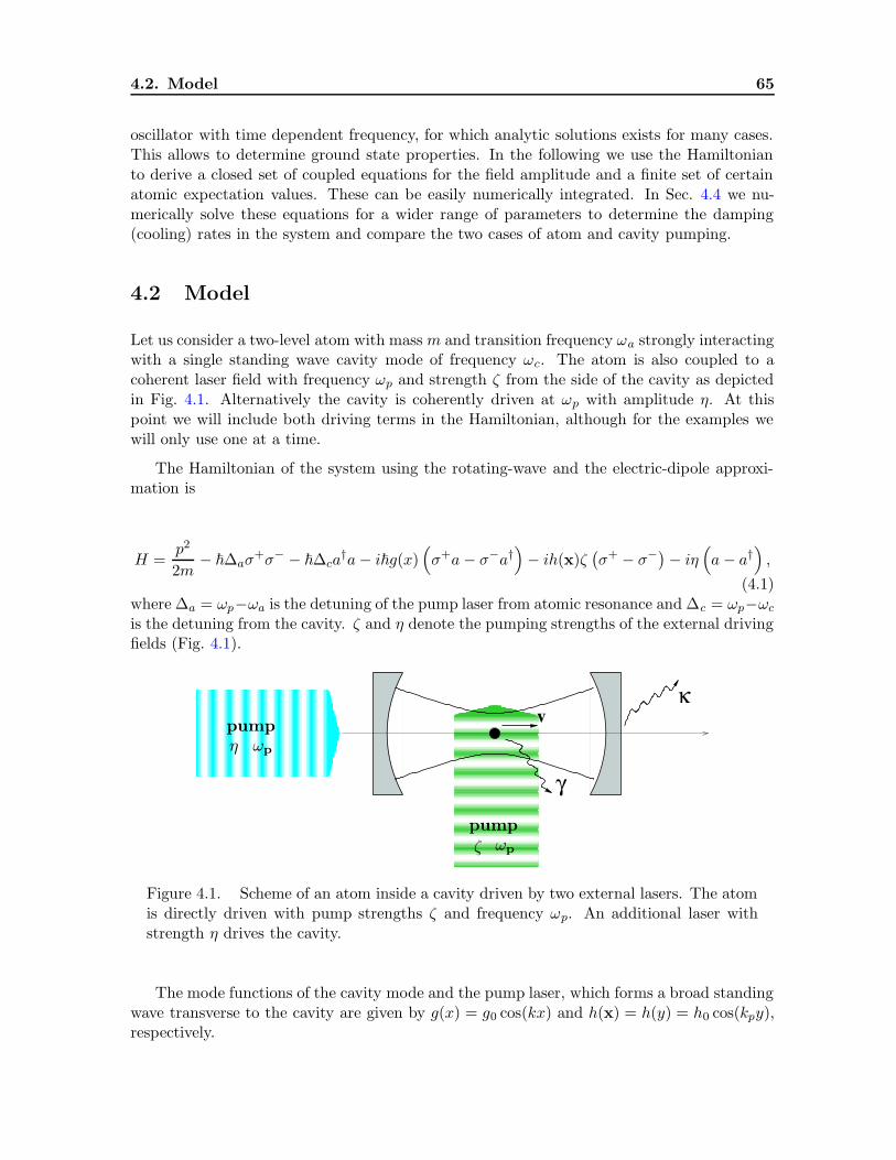
4.2. Model 65
oscillator with time dependent frequency, for which analytic solutions exists for many cases.This allows to determine ground state properties. In the following we use the Hamiltonianto derive a closed set of coupled equations for the field amplitude and a finite set of certainatomic expectation values. These can be easily numerically integrated. In Sec. 4.4 we nu-merically solve these equations for a wider range of parameters to determine the damping(cooling) rates in the system and compare the two cases of atom and cavity pumping.
4.2 Model
Let us consider a two-level atom with mass m and transition frequency ωa strongly interactingwith a single standing wave cavity mode of frequency ωc. The atom is also coupled to acoherent laser field with frequency ωp and strength ζ from the side of the cavity as depictedin Fig. 4.1. Alternatively the cavity is coherently driven at ωp with amplitude η. At thispoint we will include both driving terms in the Hamiltonian, although for the examples wewill only use one at a time.
The Hamiltonian of the system using the rotating-wave and the electric-dipole approxi-mation is
H =p2
2m− ~∆aσ
+σ− − ~∆ca†a− i~g(x)
(
σ+a− σ−a†)
− ih(x)ζ(
σ+ − σ−)
− iη(
a− a†)
,
(4.1)where ∆a = ωp−ωa is the detuning of the pump laser from atomic resonance and ∆c = ωp−ωcis the detuning from the cavity. ζ and η denote the pumping strengths of the external drivingfields (Fig. 4.1).
Figure 4.1. Scheme of an atom inside a cavity driven by two external lasers. The atomis directly driven with pump strengths ζ and frequency ωp. An additional laser withstrength η drives the cavity.
The mode functions of the cavity mode and the pump laser, which forms a broad standingwave transverse to the cavity are given by g(x) = g0 cos(kx) and h(x) = h(y) = h0 cos(kpy),respectively.
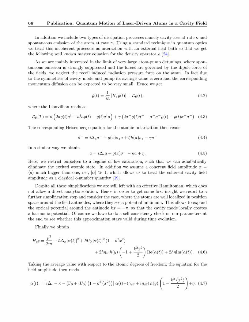
66 Publication: Quantum Motion of Laser-Driven Atoms in a Cavity Field
In addition we include two types of dissipation processes namely cavity loss at rate κ andspontaneous emission of the atom at rate γ. Using a standard technique in quantum opticswe treat this incoherent processes as interaction with an external heat bath so that we getthe following well known master equation for the density operator % [24].
As we are mainly interested in the limit of very large atom-pump detunings, where spon-taneous emission is strongly suppressed and the forces are governed by the dipole force ofthe fields, we neglect the recoil induced radiation pressure force on the atom. In fact dueto the symmetries of cavity mode and pump its average value is zero and the correspondingmomentum diffusion can be expected to be very small. Hence we get
%(t) =1
i~[H, %(t)] + L%(t), (4.2)
where the Liouvillian reads as
L%(T ) = κ(
2a%(t)a† − a†a%(t)− %(t)a†a)
+ γ(
2σ−%(t)σ+ − σ+σ−%(t)− %(t)σ+σ−)
(4.3)
The corresponding Heisenberg equation for the atomic polarization then reads
σ− = i∆aσ− + g(x)σza+ ζh(x)σz − γσ− (4.4)
In a similar way we obtain
a = i∆ca+ g(x)σ− − κa+ η. (4.5)
Here, we restrict ourselves to a regime of low saturation, such that we can adiabaticallyeliminate the excited atomic state. In addition we assume a coherent field amplitude α =〈a〉 much bigger than one, i.e., |α| 1, which allows us to treat the coherent cavity fieldamplitude as a classical c-number quantity [19].
Despite all these simplifications we are still left with an effective Hamiltonian, which doesnot allow a direct analytic solution. Hence in order to get some first insight we resort to afurther simplification step and consider the case, where the atoms are well localized in positionspace around the field antinodes, where they see a potential minimum. This allows to expandthe optical potential around the antinode kx = −π, so that the cavity mode locally createsa harmonic potential. Of course we have to do a self consistency check on our parameters atthe end to see whether this approximation stays valid during time evolution.
Finally we obtain
Heff =p2
2m− ~∆c |α(t)|2 + ~U0 |α(t)|2 (1− k2x2)
+ 2~ηeffh(y)
(
−1 +k2x2
2
)
Re(α(t)) + 2~ηIm(α(t)). (4.6)
Taking the average value with respect to the atomic degrees of freedom, the equation for thefield amplitude then reads
α(t) =[
i∆c − κ− (Γ0 + iU0)(
1− k2⟨
x2⟩)]
α(t)−(γeff + iηeff) h(y)
(
1− k2⟨
x2⟩
2
)
+η. (4.7)
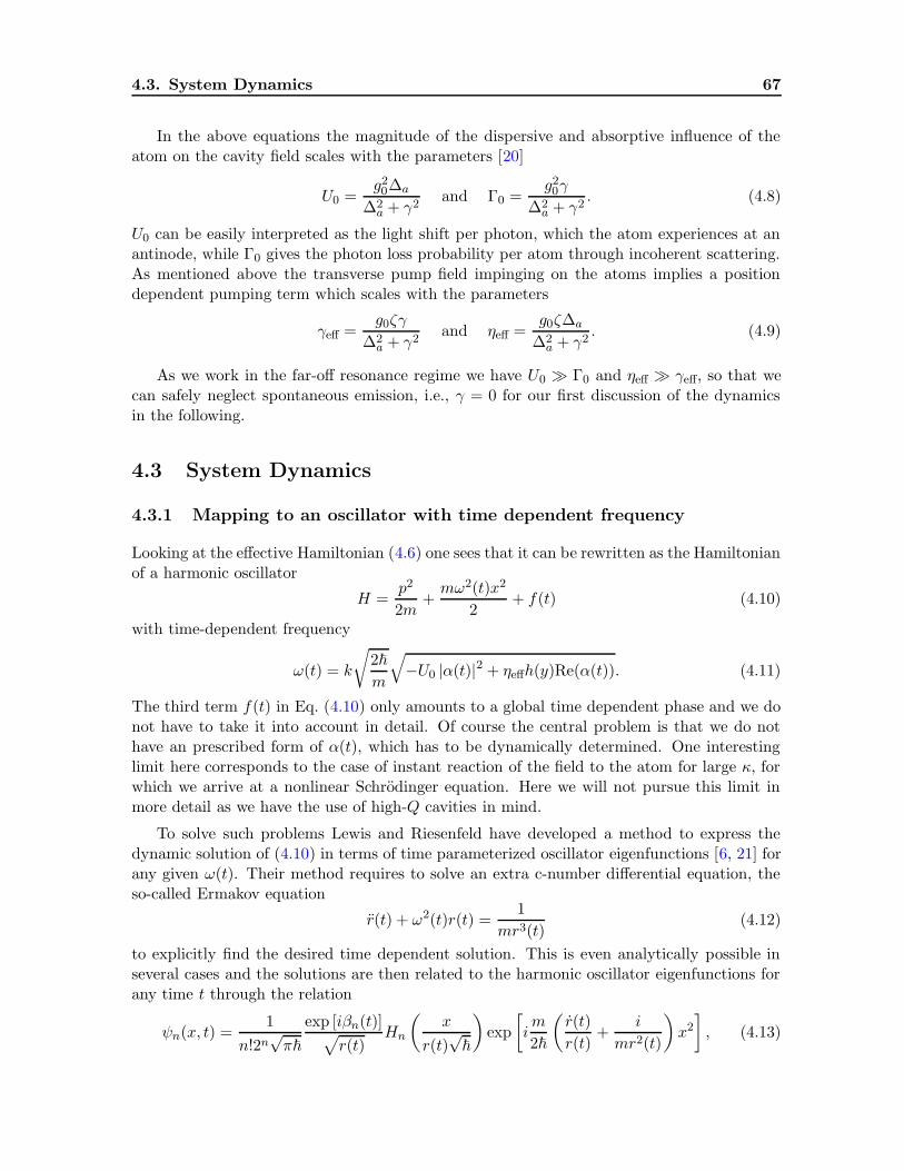
4.3. System Dynamics 67
In the above equations the magnitude of the dispersive and absorptive influence of theatom on the cavity field scales with the parameters [20]
U0 =g20∆a
∆2a + γ2
and Γ0 =g20γ
∆2a + γ2
. (4.8)
U0 can be easily interpreted as the light shift per photon, which the atom experiences at anantinode, while Γ0 gives the photon loss probability per atom through incoherent scattering.As mentioned above the transverse pump field impinging on the atoms implies a positiondependent pumping term which scales with the parameters
γeff =g0ζγ
∆2a + γ2
and ηeff =g0ζ∆a
∆2a + γ2
. (4.9)
As we work in the far-off resonance regime we have U0 Γ0 and ηeff γeff, so that wecan safely neglect spontaneous emission, i.e., γ = 0 for our first discussion of the dynamicsin the following.
4.3 System Dynamics
4.3.1 Mapping to an oscillator with time dependent frequency
Looking at the effective Hamiltonian (4.6) one sees that it can be rewritten as the Hamiltonianof a harmonic oscillator
H =p2
2m+mω2(t)x2
2+ f(t) (4.10)
with time-dependent frequency
ω(t) = k
√
2~
m
√
−U0 |α(t)|2 + ηeffh(y)Re(α(t)). (4.11)
The third term f(t) in Eq. (4.10) only amounts to a global time dependent phase and we donot have to take it into account in detail. Of course the central problem is that we do nothave an prescribed form of α(t), which has to be dynamically determined. One interestinglimit here corresponds to the case of instant reaction of the field to the atom for large κ, forwhich we arrive at a nonlinear Schrodinger equation. Here we will not pursue this limit inmore detail as we have the use of high-Q cavities in mind.
To solve such problems Lewis and Riesenfeld have developed a method to express thedynamic solution of (4.10) in terms of time parameterized oscillator eigenfunctions [6, 21] forany given ω(t). Their method requires to solve an extra c-number differential equation, theso-called Ermakov equation
r(t) + ω2(t)r(t) =1
mr3(t)(4.12)
to explicitly find the desired time dependent solution. This is even analytically possible inseveral cases and the solutions are then related to the harmonic oscillator eigenfunctions forany time t through the relation
ψn(x, t) =1
n!2n√π~
exp [iβn(t)]√
r(t)Hn
(
x
r(t)√
~
)
exp
[
im
2~
(
r(t)
r(t)+
i
mr2(t)
)
x2
]
, (4.13)

68 Publication: Quantum Motion of Laser-Driven Atoms in a Cavity Field
where βn(t) reads
βn(t) = −1
~
∫ t
0
[
~ (n+ 1/2)
mr2(t′)− f(t′)
]
dt′. (4.14)
In our case we do not have an explicit form of ω(t) and so we cannot derive an explicitanalytical answer. However, the numerical solution of the full dynamics can be simply foundby solving a single ordinary differential equation for r(t) in parallel with finding the light fielddynamics. This is fairly easily possible, as one can express the values of atomic operatorsneeded to solve the light field equation simply in terms of r(t) for any given n. If the atomis initially in the ground state ψ0(x, 0) with respect to the momentary field intensity, thisrelation reads
⟨
x2(t)⟩
=~
2r2(t) (4.15)
⟨
p2(t)⟩
=~
2r−2(t) +
~m2
2r2(t). (4.16)
Similar results hold for initial conditions of higher n. Note that due to the influenceof atomic expectation values on the field dynamics, which feed back to the atomic timeevolution, the problem is not linear. Hence if we decompose the initial condition into aharmonic oscillator basis, we cannot solve the dynamics separately for each basis state andthen add up the contributions. Instead we numerically have to find the solution independentlyfor each initial condition. From the form of the solutions one sees immediately, that the shapeof the wavefunction does not change, if one starts with an oscillator eigenfunction. An initiallyprepared Gaussian wave packet stays Gaussian all the time and only its width changes. Thisis important, if we start with a steady state and then change one of the operating parameterslike pump strength or detuning. Here the wavefunction always corresponds to the sameoscillator eigenstate and we only get a time dependent width and phase of the wavefunction.
Of course during time evolution we have to check, whether this width stays consistentwith the harmonic approximation for the potential. From the time dependent solution wecan then extract all desired quantities as the kinetic or the total mean energy of the atomto characterize the cooling and relaxation properties of our system. Of course by lookingfor solutions with time independent r we can search for steady states and find propertiesof the ground state of the coupled system. To illustrate this at an example, we solve (4.7)and (4.12) in the case where the pump light is directly applied to the atom, i.e., η = 0 andηeff 6= 0. For simplicity we start with a superposition of only few oscillator eigenstates. Asinitial basis we choose the eigenstates corresponding to the momentary eigenfrequency ω(0)derived from the chosen initial value of the field amplitude α(0).
Hence we have to set r(0) = [mω(0)]−1/2 and r(0) = 0. The operating parameters∆c = −10κ and U0 = −5κ are chosen in a way that the light field creates an attractivepotential for the atoms and we get cooling in the corresponding classical model [19]. As asimple but nontrivial example we choose an even superposition of the ground state and thefirst excited state ψ(x, 0) = 1√
2[ψ0(x, 0) + ψ1(x, 0)] and a very weak initial value of the field
α(0) = 1.
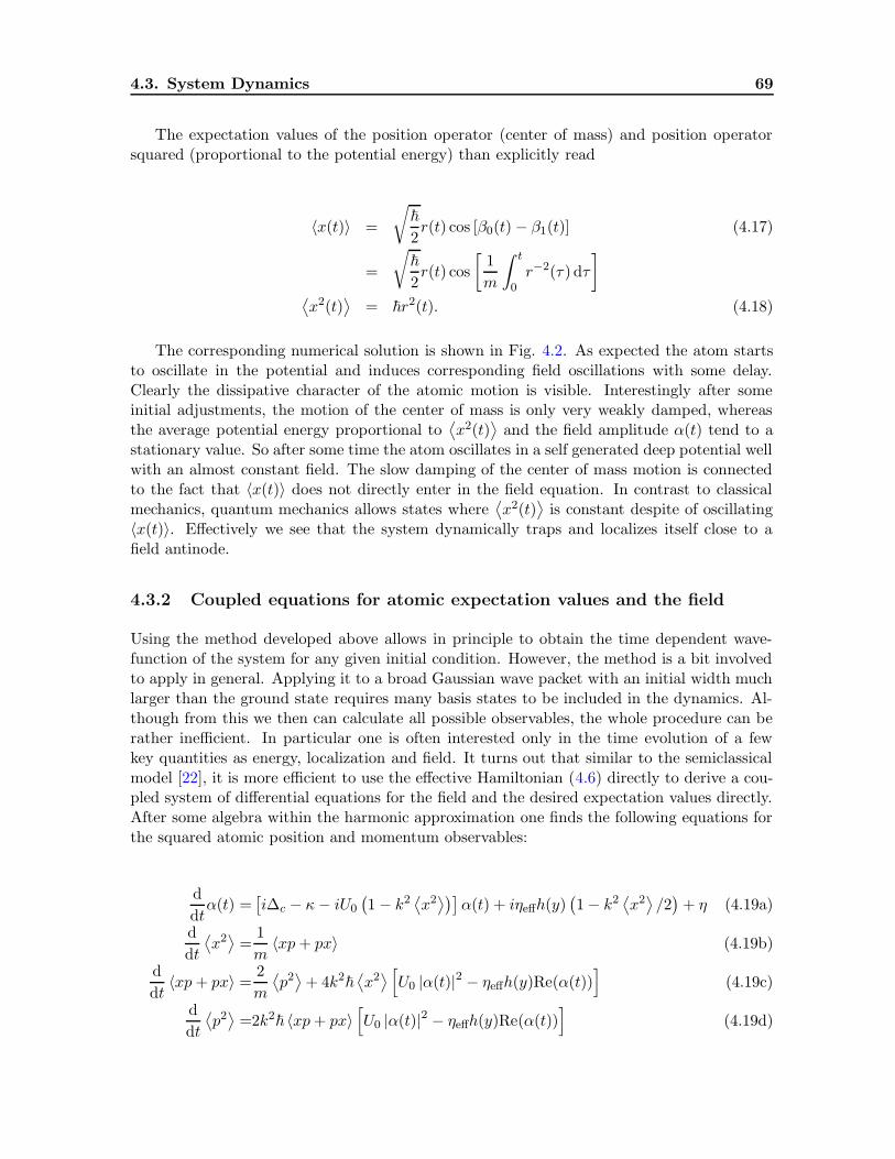
4.3. System Dynamics 69
The expectation values of the position operator (center of mass) and position operatorsquared (proportional to the potential energy) than explicitly read
〈x(t)〉 =
√
~
2r(t) cos [β0(t)− β1(t)] (4.17)
=
√
~
2r(t) cos
[
1
m
∫ t
0r−2(τ) dτ
]
⟨
x2(t)⟩
= ~r2(t). (4.18)
The corresponding numerical solution is shown in Fig. 4.2. As expected the atom startsto oscillate in the potential and induces corresponding field oscillations with some delay.Clearly the dissipative character of the atomic motion is visible. Interestingly after someinitial adjustments, the motion of the center of mass is only very weakly damped, whereasthe average potential energy proportional to
⟨
x2(t)⟩
and the field amplitude α(t) tend to astationary value. So after some time the atom oscillates in a self generated deep potential wellwith an almost constant field. The slow damping of the center of mass motion is connectedto the fact that 〈x(t)〉 does not directly enter in the field equation. In contrast to classicalmechanics, quantum mechanics allows states where
⟨
x2(t)⟩
is constant despite of oscillating〈x(t)〉. Effectively we see that the system dynamically traps and localizes itself close to afield antinode.
4.3.2 Coupled equations for atomic expectation values and the field
Using the method developed above allows in principle to obtain the time dependent wave-function of the system for any given initial condition. However, the method is a bit involvedto apply in general. Applying it to a broad Gaussian wave packet with an initial width muchlarger than the ground state requires many basis states to be included in the dynamics. Al-though from this we then can calculate all possible observables, the whole procedure can berather inefficient. In particular one is often interested only in the time evolution of a fewkey quantities as energy, localization and field. It turns out that similar to the semiclassicalmodel [22], it is more efficient to use the effective Hamiltonian (4.6) directly to derive a cou-pled system of differential equations for the field and the desired expectation values directly.After some algebra within the harmonic approximation one finds the following equations forthe squared atomic position and momentum observables:
d
dtα(t) =
[
i∆c − κ− iU0
(
1− k2⟨
x2⟩)]
α(t) + iηeffh(y)(
1− k2⟨
x2⟩
/2)
+ η (4.19a)
d
dt
⟨
x2⟩
=1
m〈xp+ px〉 (4.19b)
d
dt〈xp+ px〉 =
2
m
⟨
p2⟩
+ 4k2~⟨
x2⟩
[
U0 |α(t)|2 − ηeffh(y)Re(α(t))]
(4.19c)
d
dt
⟨
p2⟩
=2k2~ 〈xp+ px〉
[
U0 |α(t)|2 − ηeffh(y)Re(α(t))]
(4.19d)

70 Publication: Quantum Motion of Laser-Driven Atoms in a Cavity Field
Figure 4.2. Numerical solution of the field equation (4.7) and the Ermakov equa-tion (4.12) for the directly driven atom. The initially prepared state is ψ(x, 0) =1√2[ψ0(x, 0) + ψ1(x, 0)]. The parameters are κ = 1, η2
eff = 200, ∆c = −10 and U0 = −5.
Again this system is not analytically solvable, but surprisingly it is closed, finite and fairlyeasy to solve numerically, independent of the precise form of the initial wavefunction. Letus again first consider the case of coherent pumping applied directly to the atom, i.e. η = 0and ηeff 6= 0. A typical numerical solution of the time evolution is shown in Fig. 4.4. Asabove after some relaxation oscillations the system reaches a quasi steady state. Again wehave chosen parameters implying cooling in the classical case. Note that the solution obeysthe limitations set by the Heisenberg uncertainty relation in the quantum dynamics.
4.3.3 Steady state properties
Before we dicuss the parameter dependence of the dynamics in more detail, we derive somesimple results on stationary states of this system. Interestingly by setting (4.19a) and (4.19c)to zero one immediatly sees, that there is no unique solution for the steady state equations.For any given value of
⟨
x2s
⟩
exists a corresponding value of⟨
p2s
⟩
, such that the system is in asteady state. Hence we have different stable states despite the fact that the system is coupledto a zero temperature bath via the cavity modes. Only if we impose the extra condition,that the steady state is a Heisenberg limited Gaussian wave packet like the ground state ofan oscillator, the solution becomes unique and we have

4.3. System Dynamics 71
⟨
x2⟩
=b2
2and
⟨
p2⟩
=~
2
2b2, (4.20)
where b is a solution of the equation:
~
b2m= −2k2
[
U0 |αs|2 − ηeffh(y)Re(αs)]
b2. (4.21)
The corresponding stationary field amplitude then reads
αs = −i (1− k2b2/4)ηeffh(y)
i∆c − κ− iU0(1− k2b2/2). (4.22)
Figure 4.3. Width b of the stationary oscillator ground state for ∆c = −10κ, dependingon U0. The other parameters are κ = 1 and η2
eff = 200κ. The solid line corresponds tothe directly driven atom, the dashed dotted line corresponds to the laser-driven cavity.
In Fig. 4.3 we plot the width of the system ground state b as a function of the couplingstrength U0 for negative pump cavity detuning ∆c = −10κ. We see a fairly weak dependenceof b on U0 while the corresponding stationary photon number shown in Fig. 4.6 shows a sharppeak, when we hit resonance. Note, that there is only one physically acceptable solutionof (4.21). In principle this equation has two positive roots b2 but we have to exclude one ofthem, because it corresponds to a width much larger than the wavelength invalidating theharmonic approximation for the potential.
For comparison we now consider the case of cavity pumping as well, i.e., we set ηeff = 0and η 6= 0. This make the equations a bit simpler. Using (4.6) we can again derive ananalogous system of nonlinear differential equations as above.
Assuming that the stationary state is a Gaussian state with width b, we can uniquelysolve the steady state equations for b and get
~2
mb2= −2k2
~U0 |αs|2 b2. (4.23)
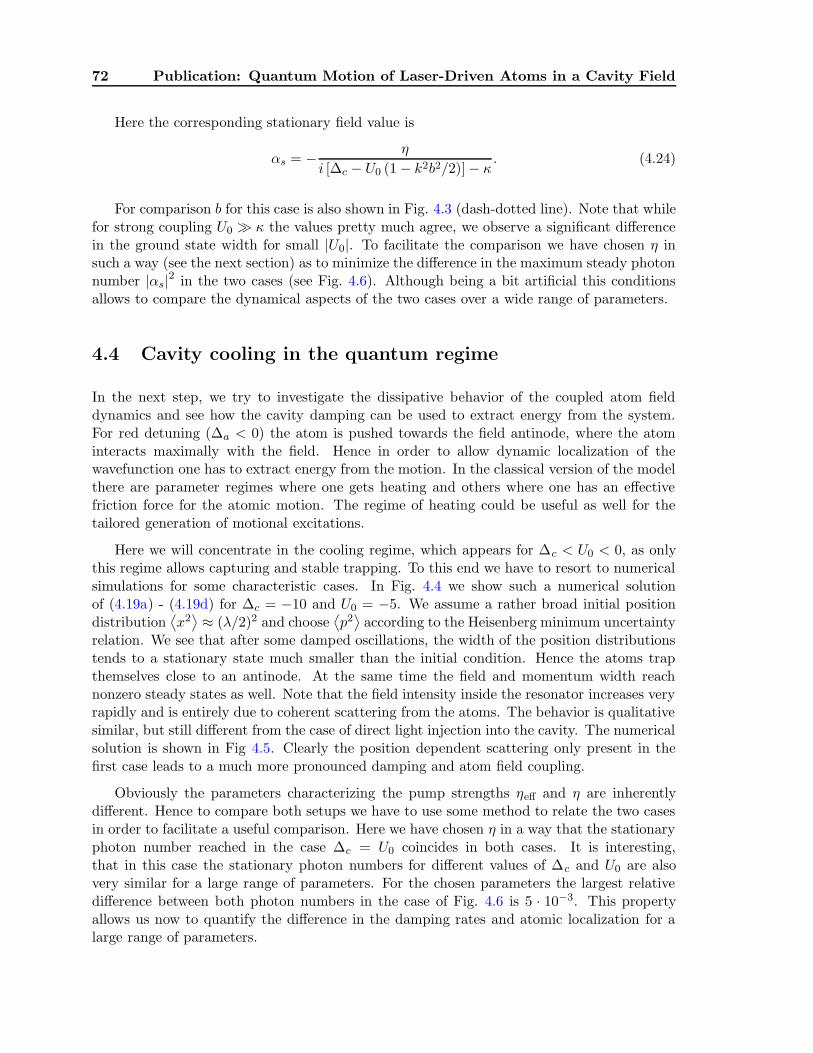
72 Publication: Quantum Motion of Laser-Driven Atoms in a Cavity Field
Here the corresponding stationary field value is
αs = − η
i [∆c − U0 (1− k2b2/2)]− κ. (4.24)
For comparison b for this case is also shown in Fig. 4.3 (dash-dotted line). Note that whilefor strong coupling U0 κ the values pretty much agree, we observe a significant differencein the ground state width for small |U0|. To facilitate the comparison we have chosen η insuch a way (see the next section) as to minimize the difference in the maximum steady photonnumber |αs|2 in the two cases (see Fig. 4.6). Although being a bit artificial this conditionsallows to compare the dynamical aspects of the two cases over a wide range of parameters.
4.4 Cavity cooling in the quantum regime
In the next step, we try to investigate the dissipative behavior of the coupled atom fielddynamics and see how the cavity damping can be used to extract energy from the system.For red detuning (∆a < 0) the atom is pushed towards the field antinode, where the atominteracts maximally with the field. Hence in order to allow dynamic localization of thewavefunction one has to extract energy from the motion. In the classical version of the modelthere are parameter regimes where one gets heating and others where one has an effectivefriction force for the atomic motion. The regime of heating could be useful as well for thetailored generation of motional excitations.
Here we will concentrate in the cooling regime, which appears for ∆c < U0 < 0, as onlythis regime allows capturing and stable trapping. To this end we have to resort to numericalsimulations for some characteristic cases. In Fig. 4.4 we show such a numerical solutionof (4.19a) - (4.19d) for ∆c = −10 and U0 = −5. We assume a rather broad initial positiondistribution
⟨
x2⟩
≈ (λ/2)2 and choose⟨
p2⟩
according to the Heisenberg minimum uncertaintyrelation. We see that after some damped oscillations, the width of the position distributionstends to a stationary state much smaller than the initial condition. Hence the atoms trapthemselves close to an antinode. At the same time the field and momentum width reachnonzero steady states as well. Note that the field intensity inside the resonator increases veryrapidly and is entirely due to coherent scattering from the atoms. The behavior is qualitativesimilar, but still different from the case of direct light injection into the cavity. The numericalsolution is shown in Fig 4.5. Clearly the position dependent scattering only present in thefirst case leads to a much more pronounced damping and atom field coupling.
Obviously the parameters characterizing the pump strengths ηeff and η are inherentlydifferent. Hence to compare both setups we have to use some method to relate the two casesin order to facilitate a useful comparison. Here we have chosen η in a way that the stationaryphoton number reached in the case ∆c = U0 coincides in both cases. It is interesting,that in this case the stationary photon numbers for different values of ∆c and U0 are alsovery similar for a large range of parameters. For the chosen parameters the largest relativedifference between both photon numbers in the case of Fig. 4.6 is 5 · 10−3. This propertyallows us now to quantify the difference in the damping rates and atomic localization for alarge range of parameters.

4.4. Cavity cooling in the quantum regime 73
Figure 4.4. Numerical Solutions for the directly driven atom. (a) Intensity |α(t)|2 ofthe cavity field and (b),(c) Variances of x and p, respectively. The parameters in thiscase are κ = 1, η2
eff = 200, ∆c = −10 and U0 = −5.
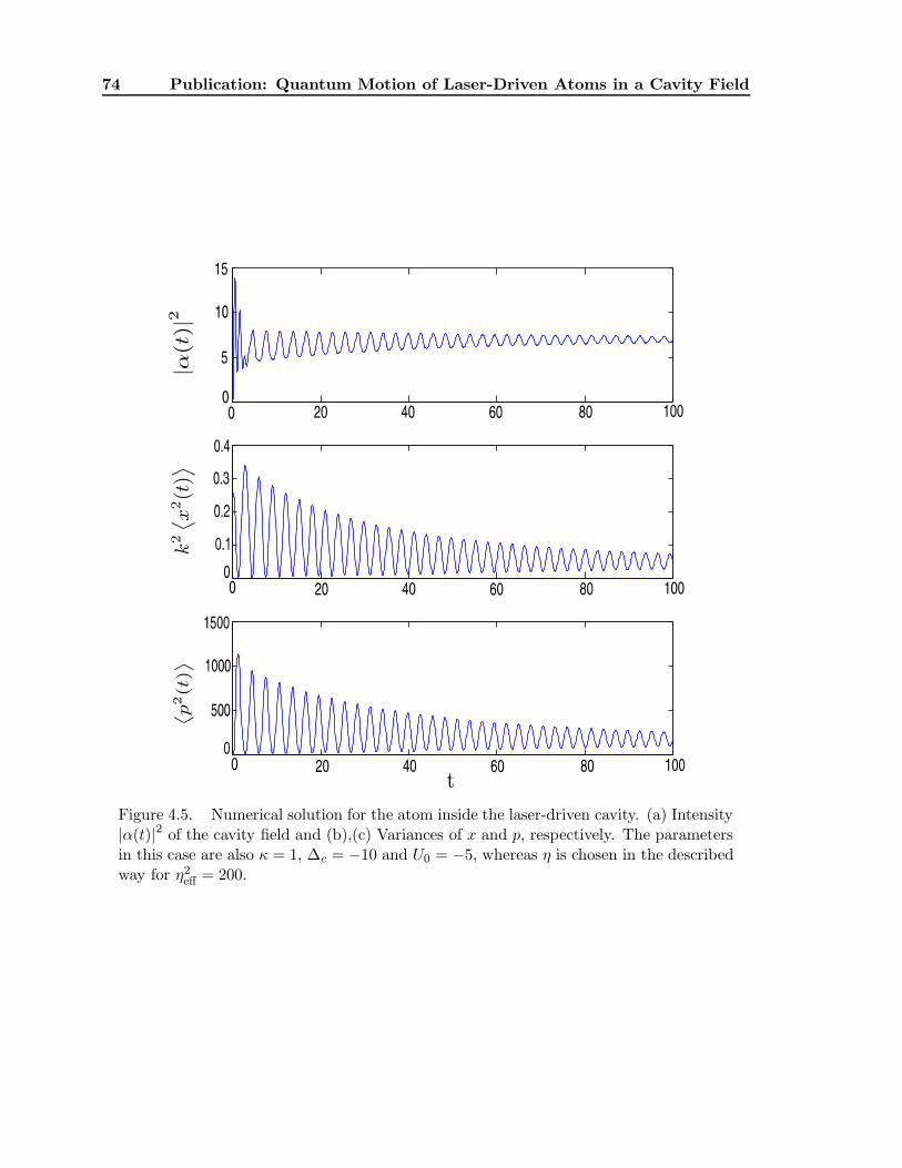
74 Publication: Quantum Motion of Laser-Driven Atoms in a Cavity Field
Figure 4.5. Numerical solution for the atom inside the laser-driven cavity. (a) Intensity|α(t)|2 of the cavity field and (b),(c) Variances of x and p, respectively. The parametersin this case are also κ = 1, ∆c = −10 and U0 = −5, whereas η is chosen in the describedway for η2
eff = 200.

4.4. Cavity cooling in the quantum regime 75
Figure 4.6. Stationary photon number |αs(t)|2 of the cavity field for the laser-drivencavity and the cavity with directly driven atom, in the case of the harmonic groundstate, whose width depends on U0 and ∆c. The parameters are κ = 1, ∆c = −10 andη2eff = 200. We choose η, such that both photon numbers coincide for ∆c = U0.
To quantify the cooling efficiency we fit the time dependence of the cycle averaged energyof the atom
E =1
2m
⟨
p2⟩
+mω2(t)
2
⟨
x2⟩
, (4.25)
to an exponential decay, from which we then read off a damping rate. Here ω(t) is thetime-dependent trap frequency. Although quantum dynamical aspects of the cavity field arein principle physically very interesting, we have to limit our parameter space here to largeenough photon numbers |αs|2 > 1 to legitimate the semiclassical approximation for the field.
Figure 4.7. Numerically calculated damping parameters for (a) ∆c = −10 and (b)∆c = −5 for the directly driven atom (solid line) and the driven cavity (dash-dottedline). The parameters are κ = 1, η2
eff = 200 and η as described in Fig. 4.6.
As obvious from Fig. 4.7 for large |∆c| we find a strong resonant enhancement of the damp-ing rate around U0 ≈ ∆c/2. In general for large detuning and large |U0| (strong coupling)the difference between driving the atom or the mode is not very pronounced. However, forsmaller |U0|, which is the regime more easily attainable experimentally, driving directly the
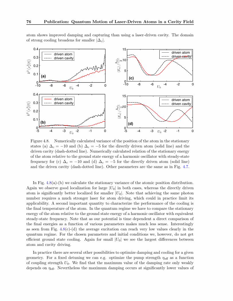
76 Publication: Quantum Motion of Laser-Driven Atoms in a Cavity Field
atom shows improved damping and capturing than using a laser-driven cavity. The domainof strong cooling broadens for smaller |∆c|.
Figure 4.8. Numerically calculated variance of the position of the atom in the stationarystates (a) ∆c = −10 and (b) ∆c = −5 for the directly driven atom (solid line) and thedriven cavity (dash-dotted line). Numerically calculated relation of the stationary energyof the atom relative to the ground state energy of a harmonic oscillator with steady-statefrequency for (c) ∆c = −10 and (d) ∆c = −5 for the directly driven atom (solid line)and the driven cavity (dash-dotted line). Other parameters are the same as in Fig. 4.7.
In Fig. 4.8(a)-(b) we calculate the stationary variance of the atomic position distribution.Again we observe good localization for large |U0| in both cases, whereas the directly drivenatom is significantly better localized for smaller |U0|. Note that achieving the same photonnumber requires a much stronger laser for atom driving, which could in practice limit itsapplicability. A second important quantity to characterize the performance of the cooling isthe final temperature of the atom. In the quantum regime we have to compare the stationaryenergy of the atom relative to the ground state energy of a harmonic oscillator with equivalentsteady-state frequency. Note that as our potential is time dependent a direct comparison ofthe final energies as a function of various parameters makes much less sense. Interestinglyas seen from Fig. 4.8(c)-(d) the average excitation can reach very low values clearly in thequantum regime. For the chosen parameters and initial conditions we, however, do not getefficient ground state cooling. Again for small |U0| we see the largest differences betweenatom and cavity driving.
In practice there are several other possibilities to optimize damping and cooling for a givengeometry. For a fixed detuning we can e.g. optimize the pump strength ηeff as a functionof coupling strength U0. We find that the maximum value of the damping rate only weaklydepends on ηeff. Nevertheless the maximum damping occurs at significantly lower values of
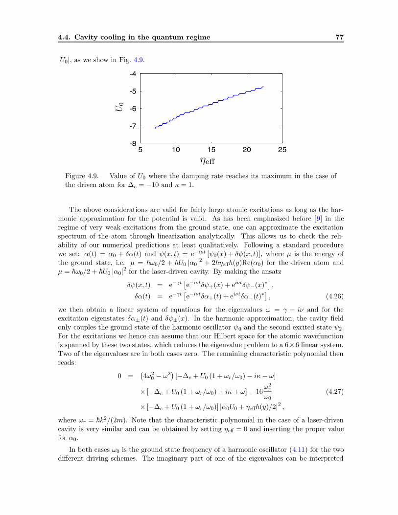
4.4. Cavity cooling in the quantum regime 77
|U0|, as we show in Fig. 4.9.
Figure 4.9. Value of U0 where the damping rate reaches its maximum in the case ofthe driven atom for ∆c = −10 and κ = 1.
The above considerations are valid for fairly large atomic excitations as long as the har-monic approximation for the potential is valid. As has been emphasized before [9] in theregime of very weak excitations from the ground state, one can approximate the excitationspectrum of the atom through linearization analytically. This allows us to check the reli-ability of our numerical predictions at least qualitatively. Following a standard procedurewe set: α(t) = α0 + δα(t) and ψ(x, t) = e−iµt [ψ0(x) + δψ(x, t)], where µ is the energy ofthe ground state, i.e. µ = ~ω0/2 + ~U0 |α0|2 + 2~ηeffh(y)Re(α0) for the driven atom andµ = ~ω0/2 + ~U0 |α0|2 for the laser-driven cavity. By making the ansatz
δψ(x, t) = e−γt[
e−iνtδψ+(x) + eiνtδψ−(x)∗]
,
δα(t) = e−γt[
e−iνtδα+(t) + eiνtδα−(t)∗]
, (4.26)
we then obtain a linear system of equations for the eigenvalues ω = γ − iν and for theexcitation eigenstates δα±(t) and δψ±(x). In the harmonic approximation, the cavity fieldonly couples the ground state of the harmonic oscillator ψ0 and the second excited state ψ2.For the excitations we hence can assume that our Hilbert space for the atomic wavefunctionis spanned by these two states, which reduces the eigenvalue problem to a 6×6 linear system.Two of the eigenvalues are in both cases zero. The remaining characteristic polynomial thenreads:
0 =(
4ω20 − ω2
)
[−∆c + U0 (1 + ωr/ω0)− iκ− ω]
× [−∆c + U0 (1 + ωr/ω0) + iκ+ ω]− 16ω2r
ω0(4.27)
× [−∆c + U0 (1 + ωr/ω0)] |α0U0 + ηeffh(y)/2|2 ,where ωr = ~k2/(2m). Note that the characteristic polynomial in the case of a laser-drivencavity is very similar and can be obtained by setting ηeff = 0 and inserting the proper valuefor α0.
In both cases ω0 is the ground state frequency of a harmonic oscillator (4.11) for the twodifferent driving schemes. The imaginary part of one of the eigenvalues can be interpreted
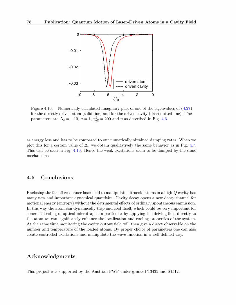
78 Publication: Quantum Motion of Laser-Driven Atoms in a Cavity Field
Figure 4.10. Numerically calculated imaginary part of one of the eigenvalues of (4.27)for the directly driven atom (solid line) and for the driven cavity (dash-dotted line). Theparameters are ∆c = −10, κ = 1, η2
eff = 200 and η as described in Fig. 4.6.
as energy loss and has to be compared to our numerically obtained damping rates. When weplot this for a certain value of ∆c we obtain qualitatively the same behavior as in Fig. 4.7.This can be seen in Fig. 4.10. Hence the weak excitations seem to be damped by the samemechanisms.
4.5 Conclusions
Enclosing the far-off resonance laser field to manipulate ultracold atoms in a high-Q cavity hasmany new and important dynamical quantities. Cavity decay opens a new decay channel formotional energy (entropy) without the detrimental effects of ordinary spontaneous emmission.In this way the atom can dynamically trap and cool itself, which could be very important forcoherent loading of optical microtraps. In particular by applying the driving field directly tothe atom we can significantly enhance the localization and cooling properties of the system.At the same time monitoring the cavity output field will then give a direct observable on thenumber and temperature of the loaded atoms. By proper choice of parameters one can alsocreate controlled excitations and manipulate the wave function in a well defined way.
Acknowledgments
This project was supported by the Austrian FWF under grants P13435 and S1512.
BIBLIOGRAPHY 79
Bibliography
[1] see e.g. Bose-Einstein Condensation, L. Pitaevskii and S. Stringari, Oxford, ClarendonPress, 2003.
[2] R. Grimm, M. Weidemller, and Yu. B. Ovchinnikov, Adv. At. Mol. Opt. Phys. 42, 95(2000).
[3] M. Greiner, O. Mandel, T. Esslinger, T.W. Hansch, and I. Bloch, Nature 415, 39 (2002).
[4] D. Jaksch , C. Bruder, J. I. Cirac, C.W. Gardiner, and P. Zoller, Phys. Rev. Lett. 81,3108 (1998).
[5] M. Holzmann and J. Audretsch, Europhys. Lett. 40, 31 (1997).
[6] H. R. Lewis and W. B. Riesenfeld, J. Math. Phys. 10, 1458 (1969).
[7] J. Stenger, S. Inouye, D.M. Stamper-Kurn, A.P. Chikkatur, D.E. Pritchard, and W.Ketterle, Appl. Phys. B 69, 347 (1999).
[8] P. Horak, G. Hechenblaikner, K. M. Gheri, H. Stecher, and H. Ritsch, Phys. Rev. Lett.79, 4974 (1997)
[9] P. Horak and H. Ritsch, Phys. Rev. A. 63, 023603(R) (2001).
[10] D. Jaksch, S. Gardiner, K . Schulze, J. Cirac, and P. Zoller, Phys. Rev. Lett. 86, 4773(2001).
[11] A. Mosk, S. Jochim, H. Moritz, Th. Elsasser, M. Weidemller, and R. Grimm, Opt. Lett.26, 1837 (2001).
[12] P. Horak, S. M. Barnett, and H. Ritsch, Phys. Rev. A 61, 033609 (2000).
[13] P. Horak and H. Ritsch, Eur. Phys. J. D 13, 279 (2001).
[14] W. Ren, J. D. Cresser, and H. J. Carmichael, Phys. Rev. A 46, 7162 (1992).
[15] P. Domokos and H. Ritsch, Phys. Rev. Lett. 89, 253003, (2002).
[16] H. W. Chan, A.T. Black, and V. Vuletic, Phys. Rev. Lett. 90, 063003 (2003).
[17] D. Kruse, C. von Cube, C. Zimmermann, and P. W. Courteille, Phys. Rev. Lett. 91,183601 (2003).
[18] B. Nagorny, T. Elsasser, and A. Hemmerich, Phys. Rev. Lett. 91, 153003 (2003).
[19] P. Domokos, P. Horak, and H. Ritsch, J. Phys. B 34, (2001).
[20] P. Domokos and H. Ritsch, J. Opt. Soc. Am. B 20, 1098 (2003).
[21] I. A. Pedrosa, Phys. Rev. A. 55, 3219 (1997).
[22] M. Gangl and H. Ritsch, Phys. Rev. A. 61, 011402(R) (2000).
80 Publication: Quantum Motion of Laser-Driven Atoms in a Cavity Field
[23] P. Maunz, T. Puppe, I. Schuster, N. Syassen, P. W. H. Pinkse, and G. Rempe, Nature428, 50 (2004).
[24] C. W. Gardiner, P. Zoller, Quantum noise 2nd Ed., Springer, Berlin (2000).
Chapter 5
Publication
Cold Atom Dynamics in a Quantum Optical Lattice Potential†
Physical Review Letters 95, 260401 (2005)
C. Maschler and H. Ritsch
Institut fur theoretische Physik, Universitat Innsbruck,A-6020 Innsbruck, Austria
We study a generalized cold atom Bose Hubbard model, where the periodic opticalpotential is formed by a cavity field with quantum properties. On the one hand thecommon coupling of all atoms to the same mode introduces cavity mediated long rangeatom-atom interactions and on the other hand atomic backaction on the field introducesatom-field entanglement. This modifies the properties of the associated quantum phasetransitions and allows for new correlated atom-field states including superposition ofdifferent atomic quantum phases. After deriving an approximative Hamiltonian includingthe new long range interaction terms we exhibit central physical phenomena at genericconfigurations of few atoms in few wells. We find strong modifications of populationfluctuations and next-nearest neighbor correlations near the phase transition point.
Laser fields can nowadays be routinely used to create tailored optical potentials for ultra-cold neutral atoms [1]. Loading an atomic BEC into such a periodic standing light patternallows to experimentally implement systems, which are well described by a Bose HubbardHamiltonian with externally controllable parameters [2–4]. In some recent spectacular ex-periments the predicted Mott-insulator to superfluid quantum phase transition has beenobserved [5]. As the light fields are normally intense and strongly detuned from any atomictransition, their properties can be safely approximated by prescribed classical fields inde-pendent of the atomic state. However, this is invalid if they are confined within an opticalresonator. For a sufficient atom number N and atom-field coupling g the fields become dy-namical quantities depending on the atoms. In addition in a high-Q cavity the quantumproperties of the field get important and the atoms move in quantized potentials [6, 7]. Ul-timately this allows different states of the lattice field (e.g. different photon numbers) to bequantum correlated with different quantum phases of the atoms. As a striking example theatoms could be in a superposition of a Mott insulator and a superfluid state connected witha different cavity field amplitudes. Even in the classical field limit of high photon numbersall atoms see the same field state and thus we get new long range atom-atom interactions.
†The author of the present thesis performed all the calculations in this publication.

82 Publication: Cold Atom Dynamics in a Quantum Optical Lattice Potential
Figure 5.1. Sketch of the setup. N two-level atoms, strongly interacting with a singlestanding wave mode of an optical cavity, are coherently driven by a laser field via thecavity mirrors.
Interestingly the idea of implementing such combination of cavity QED and a BEC has exper-imentally made such rapid progress recently, that its success can be expected very soon [8].
In this work we discuss the basic physical properties of such a generalized model ofultracold atoms in a periodic potential generated by a quantized field mode. In a first stepwe derive an approximate Hamiltonian analogous to the Bose Hubbard Hamiltonian includinga quantized potential. Its basic physical implications are then exhibited in two cases: (a)a strongly damped cavity, where the field dynamics can be adiabatically eliminated, whichleads to a rescaling of the coupling parameters and new long range atom-atom coupling termsand (b) a dynamical model where the field is approximated by its time dependent expectationvalue derived from a dynamical equation containing atomic expectation values.
Model: Let us consider N two-level atoms with mass m and transition frequency ωastrongly interacting with a single standing wave cavity mode of frequency ωc ωa. Thesystem is coherently driven by a laser field with frequency ωp ≈ ωc through the cavity mirrorwith amplitude η. Alternatively the atoms are illuminated transversally to the cavity axes(see Fig. 5.1) with amplitude ζ.
Including damping, the dynamics is given by the master equation for the atom field densityoperator % = 1
i~ [H, %]+L%, where the Liouvillian L models dissipation. For large atom-pumpdetuning spontaneous emission is negligible and cavity loss κ will be the dominant dissipativeprocess, i.e., L% = κ
(
2a%a† − a†a%− %a†a)
. Here a is the annihilation operator for a cavityphoton.
As convenient choice we rewrite the Hamiltonian in a second quantized form, where thedirect interaction between the atoms is modeled by a pseudopotential and characterized bythe s-wave scattering length as:

83
H =
∫
d3xΨ† (x)H0Ψ(x) +1
2
4πas~2
m
∫
d3xΨ† (x)Ψ† (x) Ψ (x) Ψ (x) . (5.1)
Here Ψ (x) is the field operator for the atoms and H0 is the single-particle Hamiltonianin rotating-wave and dipole approximation:
H0 =p2
2m− ~∆aσ
+σ− − ~∆ca†a− i~g(x)
(
σ+a− σ−a†)
− i~h (x) ζ(
σ+ − σ−)
− i~η(
a− a†)
, (5.2)
where ∆a = ωp − ωa and ∆c = ωp − ωc is the atom-pump and cavity-pump detuning,respectively. Along the cavity axis (x-direction) the atom-field coupling is set to g(x) =g0 cos(kx), while the transverse laser beam forms a standing wave with amplitude h (x) =h0 cos(kpy) in the y-direction, where we set y = 0 for our 1D-considerations. In the regime oflow saturation [9] (large ∆a) adiabatic elimination of the excited atomic state in (5.2) thenleads to:
H0 =p2
2m+cos2(kx)
(
~U0a†a+ Vcl
)
−~∆ca†a− i~η
(
a− a†)
+~ηeff cos(kx)(
a+ a†)
. (5.3)
The important parameter U0 = g20/∆a here is the optical lattice depth per photon [6]
and also gives the refractive index of one atom at an antinode. The term containing ηeff =g0h0ζ/∆a represents an effective pump through atomic scattering into the mode. Along xthe cavity field forms an optical lattice potential with period λ/2 and depth ~U0a
†a. For thesake of generality we add an extra classical potential Vcl as well.
To derive a generalized Bose-Hubbard Hamiltonian we expand the Bloch states of a singleatom inside the lattice using localized Wannier functions [10] and rewrite the field operatorsin Eq. (5.1) in these functions, keeping only the lowest vibrational state at each site (lowestband) Ψ (x) =
∑
i biw (x− xi) to get:
H =∑
k,l
Ek,lb†kbl +
(
~U0a†a+ Vcl
)
∑
k,l
Jk,lb†kbl + ~ηeff
(
a+ a†)
∑
k,l
Jk,lb†kbl − i~η
(
a− a†)
+U
2
∑
k
b†kbk(
b†kbk − 1)
− ~∆ca†a. (5.4)
The operators b†k (bk) correspond to the creation (annihilation) of an atom at site k and
the on-site interaction of two atoms is given by U = 4πas~2
m
∫
d3x |(x)|4 . As the nonlinearpart of the nearest-neighbor interaction is typically two orders of magnitude smaller thanthe on-site interaction it is neglected as usually. In contrast to the classical field case [3] theappearance of the cavity field operator does not allow to reassemble all hopping terms toa single expression. To be still able to proceed analytically we assume a weak dependence
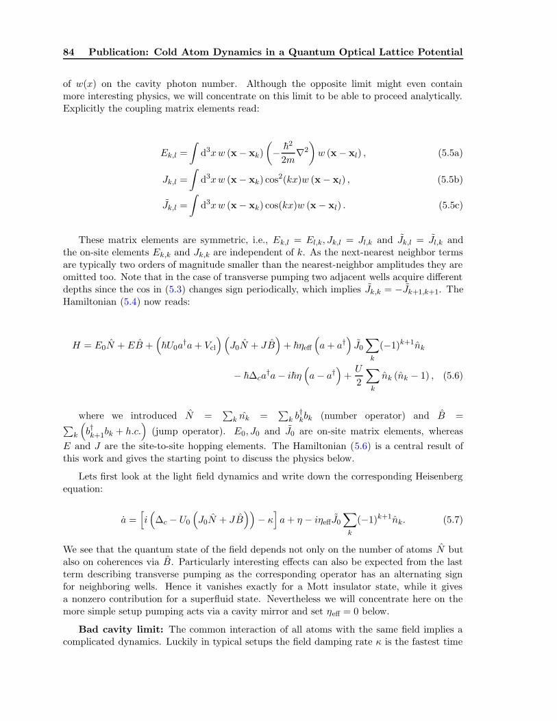
84 Publication: Cold Atom Dynamics in a Quantum Optical Lattice Potential
of w(x) on the cavity photon number. Although the opposite limit might even containmore interesting physics, we will concentrate on this limit to be able to proceed analytically.Explicitly the coupling matrix elements read:
Ek,l =
∫
d3xw (x− xk)
(
− ~2
2m∇2
)
w (x− xl) , (5.5a)
Jk,l =
∫
d3xw (x− xk) cos2(kx)w (x− xl) , (5.5b)
Jk,l =
∫
d3xw (x− xk) cos(kx)w (x− xl) . (5.5c)
These matrix elements are symmetric, i.e., Ek,l = El,k, Jk,l = Jl,k and Jk,l = Jl,k andthe on-site elements Ek,k and Jk,k are independent of k. As the next-nearest neighbor termsare typically two orders of magnitude smaller than the nearest-neighbor amplitudes they areomitted too. Note that in the case of transverse pumping two adjacent wells acquire differentdepths since the cos in (5.3) changes sign periodically, which implies Jk,k = −Jk+1,k+1. TheHamiltonian (5.4) now reads:
H = E0N +EB +(
~U0a†a+ Vcl
)(
J0N + JB)
+ ~ηeff
(
a+ a†)
J0
∑
k
(−1)k+1nk
− ~∆ca†a− i~η
(
a− a†)
+U
2
∑
k
nk (nk − 1) , (5.6)
where we introduced N =∑
k nk =∑
k b†kbk (number operator) and B =
∑
k
(
b†k+1bk + h.c.)
(jump operator). E0, J0 and J0 are on-site matrix elements, whereas
E and J are the site-to-site hopping elements. The Hamiltonian (5.6) is a central result ofthis work and gives the starting point to discuss the physics below.
Lets first look at the light field dynamics and write down the corresponding Heisenbergequation:
a =[
i(
∆c − U0
(
J0N + JB))
− κ]
a+ η − iηeffJ0
∑
k
(−1)k+1nk. (5.7)
We see that the quantum state of the field depends not only on the number of atoms N butalso on coherences via B. Particularly interesting effects can also be expected from the lastterm describing transverse pumping as the corresponding operator has an alternating signfor neighboring wells. Hence it vanishes exactly for a Mott insulator state, while it givesa nonzero contribution for a superfluid state. Nevertheless we will concentrate here on themore simple setup pumping acts via a cavity mirror and set ηeff = 0 below.
Bad cavity limit: The common interaction of all atoms with the same field implies acomplicated dynamics. Luckily in typical setups the field damping rate κ is the fastest time

85
Figure 5.2. (a) Numerically found average potential depth Veff = Vcl + ~U0〈a†a〉 of theground state of (5.6) for N = 2 atoms in two wells. (b) Relative error in this potentialusing expansion (5.9). The parameters are η = 2κ, Vcl = −4ER and the scattering lengthis as = 0.1ER.
scale in the system. This allows to eliminate the cavity degrees of freedom by formally solvingequation (5.7) for a = η/[κ − i(∆c − U0(J0N + JB))] and inserting this back to (5.4). AsN commutes with B this gives no ordering problem. For a fixed atom number N = 〈N〉 wethen expand a to second order in the small tunneling matrix element J :
a ≈ η
κ− i∆′c
[
1− iU0J
κ− i∆′c
B − U20J
2
(κ− i∆′c)
2B2
]
, (5.8)
where ∆′c = ∆c − U0J0N is a rescaled detuning, so that we have:
H =
[
E + J
(
Vcl − ~U0η2 κ2 −∆′
c2
(
κ2 + ∆′c2)2
)]
B − 3~U20 η
2∆′c
3κ2 −∆′c2
(
κ2 + ∆′c2)3 J
2B2
+U
2
∑
k
nk (nk − 1) . (5.9)
Obviously H now contains cavity induced rescaling of the tunnel coupling proportionalto B as well as nonlocal correlated two atom hopping terms proportional to B2 mediatinglong range interactions. In Fig. 5.2 we show the excellent agreement of the field calculatedfrom the expansion (5.8) compared to a full numerical inversion within a large parameterrange as used below. Note that the matrix elements still weakly depend on the depth of theoptical potential via 〈B〉 but as J is small they can be approximated neglecting the B-termand setting J0 = 1 in the field expectation value α0 = η/[κ − i(∆c −NU0)].
Lets now discuss some key physics. In the simplest case of a single particle in two wellsthe symmetric and antisymmetric superpositions of the atom in either site are eigenstateswith an energy difference
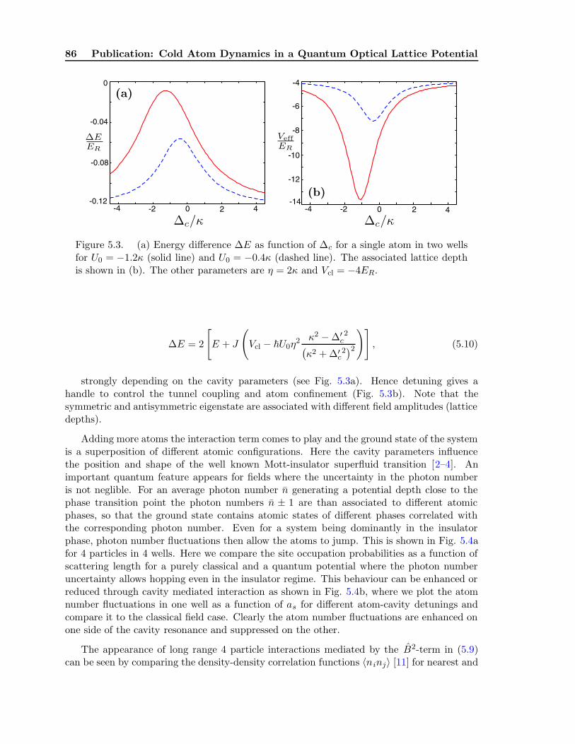
86 Publication: Cold Atom Dynamics in a Quantum Optical Lattice Potential
Figure 5.3. (a) Energy difference ∆E as function of ∆c for a single atom in two wellsfor U0 = −1.2κ (solid line) and U0 = −0.4κ (dashed line). The associated lattice depthis shown in (b). The other parameters are η = 2κ and Vcl = −4ER.
∆E = 2
[
E + J
(
Vcl − ~U0η2 κ2 −∆′
c2
(
κ2 + ∆′c2)2
)]
, (5.10)
strongly depending on the cavity parameters (see Fig. 5.3a). Hence detuning gives ahandle to control the tunnel coupling and atom confinement (Fig. 5.3b). Note that thesymmetric and antisymmetric eigenstate are associated with different field amplitudes (latticedepths).
Adding more atoms the interaction term comes to play and the ground state of the systemis a superposition of different atomic configurations. Here the cavity parameters influencethe position and shape of the well known Mott-insulator superfluid transition [2–4]. Animportant quantum feature appears for fields where the uncertainty in the photon numberis not neglible. For an average photon number n generating a potential depth close to thephase transition point the photon numbers n ± 1 are than associated to different atomicphases, so that the ground state contains atomic states of different phases correlated withthe corresponding photon number. Even for a system being dominantly in the insulatorphase, photon number fluctuations then allow the atoms to jump. This is shown in Fig. 5.4afor 4 particles in 4 wells. Here we compare the site occupation probabilities as a function ofscattering length for a purely classical and a quantum potential where the photon numberuncertainty allows hopping even in the insulator regime. This behaviour can be enhanced orreduced through cavity mediated interaction as shown in Fig. 5.4b, where we plot the atomnumber fluctuations in one well as a function of as for different atom-cavity detunings andcompare it to the classical field case. Clearly the atom number fluctuations are enhanced onone side of the cavity resonance and suppressed on the other.
The appearance of long range 4 particle interactions mediated by the B2-term in (5.9)can be seen by comparing the density-density correlation functions 〈ninj〉 [11] for nearest and

87
Figure 5.4. (a) Occupation probabilities pi for i atoms in one well as function ofscattering length for the ground state of 4 atoms in 4 wells. The parameters are U0 = −κand ∆c = −3.75κ and Veff = ~U0〈a†a〉 = −4ER. For comparison the dashed linescorrespond to an equivalent classical potential, i.e., 〈a†a〉 = 0 and Vcl = −4ER. (b)Fluctuations of atom number in one well as a function of as for different cavity detunings∆c = −5κ (solid line), ∆c = −3κ (dashed line) and a classical field (dashed-dotted line).
next nearest neighbor sites. Depending on cavity parameters as shown in Fig. 5.5a each ofthe two correlations can be enhanced or reduced with respect to the classical potential case.
Coupled atom-field dynamics in the semiclassical limit: As final point we turnto the classical field limit of the coupled Hamiltonian (5.6) for fixed N and large photonnumber. Here the field is approximately in a coherent state |α〉 and the system is assumedto evolve as a product state |Φ〉 = |ψ〉 ⊗ |α(t)〉. The Heisenberg equation (5.7) for the fieldthen reduces to a classical equation for α containing expectation values of atomic operators:
α(t) =[
i(
∆c − U0〈ψ|J0N + JB|ψ〉)
− κ]
α(t) + η, (5.11a)
i~d
dt|ψ〉 =
[
E + J(
Vcl + ~U0 |α(t)|2)]
B|ψ〉+ U
2
∑
k
nk (nk − 1) |ψ〉. (5.11b)
α(t) is then inserted back into the atomic Hamiltonian like a classical time dependentpotential Vcl [9, 12]. Similar to the case of a time dependent Gross-Pitaevskii equation [12] thecorresponding Schrodinger equation can be solved simultaneously, where the matrix elementsE, J have to be recalculated in each time step.
Although the factorizing assumption is in general doubtful and one has to check thedynamical restriction to the lowest band, this procedure gives a first insight in the dynamicalbehavior of the model. As a generic example we show the time evolution of the uncertaintyof the site occupation number starting with a ’superfluid’ state at t = 0, when the onsiteinteraction is turned on. Fig. 5.5b shows that in contrast to a fixed external potential thedynamic cavity field leads to a damping of the fluctuations approaching a Mott insulatorstate.

88 Publication: Cold Atom Dynamics in a Quantum Optical Lattice Potential
Figure 5.5. (a) Difference of the density-density correlation functions: 〈n1n3〉−〈n1n2〉.Parameters are as in Fig. 5.4b. (b) Dynamical evolution of atom number fluctuations inone well starting from an interaction free ground state and a sudden turn on of onsite-interaction. A linear fit is depicted by the dashed line. Here we chose U0 = −κ, ∆c =−4.2κ, Vcl = 0, as = 3ER and η such that Veff = −4ER.
In summary we have shown that a dynamical quantum optical potential for ultracoldatoms invokes a wealth of new physics. The effects are pronounced in the limit of strongcoupling and small photon numbers but long range interactions persist even in the bad cavitylimit within a classical field approximation. The considered systems are in range of currentexperimental capabilities and should allow to control and study new quantum phases.
Acknowledgments: We thank G. Moriggi, M. Lewenstein and P. Domokos for helpfuldiscussions. Funded by the Austrian Science Fund FWF - P17708.
Bibliography
[1] See e.g. Laser Manipulation of Atoms and Ions, ed. by E. Arimondo and W. D.Phillips,Varenna Summer School, 1991 (North-Holland, Amsterdam 1992).
[2] M. P. A. Fisher et al., Phys. Rev. B 40, 546 (1989).
[3] D. Jaksch et al., Phys. Rev. Lett. 81, 3108 (1998); D. Jaksch and P. Zoller, Ann. Phys.315, 52 (2005).
[4] W. Zwerger, J. Opt. B 5, S9 (2003).
[5] M. Greiner et al., Nature 415, 39 (2002).
[6] P. Domokos and H. Ritsch, J. Opt. Soc. Am. B 20, 1098 (2003).
[7] A. Griessner, D. Jaksch, and P. Zoller, J. Phys. B 37, 1419 (2004).
[8] B. Nagorny, T. Elsasser, and A. Hemmerich, Phys. Rev. Lett. 91, 153003 (2003); J. A.Sauer et al., Phys. Rev. A 69, 051804 (2004).

BIBLIOGRAPHY 89
[9] C. Maschler and H. Ritsch, Opt. Comm. 243, 145 (2004).
[10] C. Kittel, Quantum Theory of Solids, John Wiley & Sons, (New York 1963).
[11] T. D. Kuhner, S. R. White, and H. Monien, Phys. Rev. B 61, 12474 (2000).
[12] P. Horak and H. Ritsch, Phys. Rev. A 63, 23603 (2001).

Chapter 6
Publication
Ultracold Atoms in Optical Lattices Generated by Quantized
Light Fields†
arXiv: quant-ph/0710.4220 (submitted to European Journal of Physics D)
C. Maschler1, I. B. Mekhov1,2, and H. Ritsch1
1) Institut fur theoretische Physik, Universitat Innsbruck,A-6020 Innsbruck, Austria
2) St. Petersburg State University, Faculty of Physics,St. Petersburg, Russia
We study an ultracold gas of neutral atoms subject to the periodic optical potentialgenerated by a high-Q cavity mode. In the limit of very low temperatures, cavity fieldand atomic dynamics require a quantum description. Starting from a cavity QED singleatom Hamiltonian we use different routes to derive approximative multiparticle Hamilto-nians in Bose-Hubbard form with rescaled or even dynamical parameters. In the limit oflarge enough cavity damping the different models agree. Compared to free space opticallattices, quantum uncertainties of the potential and the possibility of atom-field entangle-ment lead to modified phase transition characteristics, the appearance of new phases oreven quantum superpositions of different phases. Using a corresponding effective masterequation, which can be numerically solved for few particles, we can study time evolutionincluding dissipation. As an example we exhibit the microscopic processes behind thetransition dynamics from a Mott insulator like state to a self-ordered superradiant stateof the atoms, which appears as steady state for transverse atomic pumping.
6.1 Introduction
Laser light, far red detuned from an atomic resonance, is nowadays a standard tool in ex-perimental quantum optics to create tunable optical potentials [1] which can be loaded withultracold atoms to provide for a plethora of possibilities to study quantum properties ofmany-body strongly correlated systems [2]. The high level of microscopic understanding andextensive control of the light fields and atoms allow to implement genuine models like e.g.the Bose-Hubbard (BH) model [3, 4]. Initially originating from condensed matter physics [5]
†The author of the present thesis performed all the calculations in this publication. I. M. acted as adiscussion partner of all the aspects of this work.

92 Publication: Ultracold Atoms in Optical Lattices Generated by . . .
it has been used to study the Mott insulator to superfluid phase transition [6] in detail and inreal time. Adjusting several of the lattice parameters as the intensity and the configurationof the lattice lasers provides a versatile toolbox of techniques to control the dynamics of theatoms in the lattice [7]. Moreover, the collisional properties of the certain types of atomscan be tailored by means of magnetic [8] or optical [9] Feshbach resonances. Using extraconfinement it was even possible to observe the Mott insulator to superfluid transition in1D [10, 11] and 2D [12], followed by other spectacular demonstrations of condensed matterphysics phenomena as the realization of a Tonks gas in 1D [13, 14] and the Berezinskii-Kosterlitz-Thouless phase transition in 2D [15]. Theoretically many more proposals to applythese methods to spin systems and investigate further fascinating properties of strongly cor-related systems were put forward (see [16] for a review).
In all of these approaches, the light fields were approximated by classical, externallyprescribed fields independent of the atoms. This requires intense light, far detuned from anyatomic transition. Of course this assumption holds no longer if the light, which generatesthe optical lattice, is enhanced by an optical resonator. In this case - given a sufficient atomnumber N and atom-field coupling g - the field itself becomes a dynamical quantity [17]depending on the atomic distribution. As all atoms are coupled to the same field modes, thisimmediately introduces substantial long range interactions, which cannot be ignored as in freespace. In specially designed cases this force induces coherently driven atoms to self-organizein regular patterns as predicted in Ref. [18, 19] and subsequently experimentally verified [20].
In addition, in a high-Q optical resonator relatively low photon numbers are sufficient toinduce strong forces. This was demonstrated by trapping an atom in the field of just a singlephoton [21, 22]. Hence the inevitable photon number fluctuations induced by cavity dampinginduce force fluctuations on the atoms inducing diffusion. At the same time as cavity photonloss constitutes a dissipation channel, it can also carry out energy and entropy of the system.This opens possibilities for cooling of atomic motion [23–26], as demonstrated by beautifulexperiments in the group of Rempe [27, 28]. Since this cooling mechanism does not requirethe existence of closed optical cycles it could even be used for qubits [29] or to damp quantumoscillations or phase fluctuations of a BEC coupled to a cavity field [30, 31].
For low photon numbers the quantum properties of the light field get important as well andthe atoms are now moving in different quantized potentials determined by the cavity photonnumber. Quantum mechanics of course allows for superpositions of photon numbers invokingsuperpositions of different optical potentials for the atoms. First simplified models to describethis new physics were recently proposed by us [32] and in parallel by other authors [33]. Asthe intracavity field itself depends on the atomic state (phase), different atomic quantumstates are correlated with different states of the lattice field with differing photon numberdistributions. In this way quantum mechanics allows for the creation of very exotic atom-fieldstates, like a superposition of a Mott-insulator and superfluid phase, each thereof correlatedwith a different photon number. Some quite exotic looking phase diagrams for this systemwere already discussed in Ref. [33]. Without resorting to the full complex dynamics of thesystem, the quantum correlations between the field and the atomic wavefunctions open thepossibility of non-destructively probing the atomic state by weak scattering of coherent lightinto the cavity mode [34] and carefully analyzing its properties [35].
It is quite astonishing, that experimental progress in the recent years has made such sys-tems experimentally accessible and at present already several experimental groups succeeded

6.2. Model 93
in loading a BEC into a high-Q optical cavity [36–39]. A reliable analysis of these experimentshas made more thorough theoretical studies of systems mandatory.
In this work we concentrate on the study of an ultracold gas in optical lattices includingthe quantum nature of the lattice potential generated from a cavity field. This extends andsubstantiates previous studies and predictions on such a system by us [32] as well as otherauthors [33]. Here we limit ourselves to the case of a high-Q cavity which strongly enhancesa field sufficiently red detuned from any atomic transition to induce an optical potentialwithout significant spontaneous emission. In particular we address two different geometricsetups, where either the cavity mode is directly driven through one mirror, or the atoms arecoherently excited by a laser and scatter light into the cavity mode. The cavity potentialcan also be additionally enhanced by some extra conservative potential applied at a differentfrequency [40, 41]. These two generic cases leads to quite different physical behavior andallow to discuss several important aspects of the underlying physics.
This paper is organized as follows. Sec. 6.2 is devoted to a systematic presentation of ourmodel and various simplifying approximations as adiabatic elimination of the excited statesof the atoms and subsequent formulation of an effective multi-particle Hamiltonian in secondquantized form. In section 6.3, we specialize on the simplest generic case of a coherentlydriven cavity and approximate the corresponding Hamiltonian by adiabatic elimination ofthe cavity field. We investigate the properties thereof, corresponding to the influence of thecavity on the Mott-insulator to superfluid quantum phase-transition and identify the regimeof validity for the elimination of the cavity field. Finally, we compare these results with thedynamics of the full master equation. In Sec. 6.4 we study the more complex case of atomscoherently driven by a laser field transversal to the cavity axis, where it is much harder tofind valid analytical simplifications and one has to resort to numerical studies of few particledynamics. Finally, we conclude in Sec. 6.5.
6.2 Model
We start with N two-level atoms with mass m and transition frequency ωeg strongly inter-acting with a single standing wave cavity mode of frequency ωc. We also consider coherentdriving of the atoms at frequency ωp and strength ζ and the cavity with amplitude η (seeFig. 6.1). Note that in the specific examples later we will consider only one pump laser beamat a time.
Using the rotating-wave and electric-dipole approximation, we can describe a single atomof this system by the Jaynes-Cummings Hamiltonian [42]
H(1) = H(1)A +H
(1)R +H
(1)Int. (6.1)
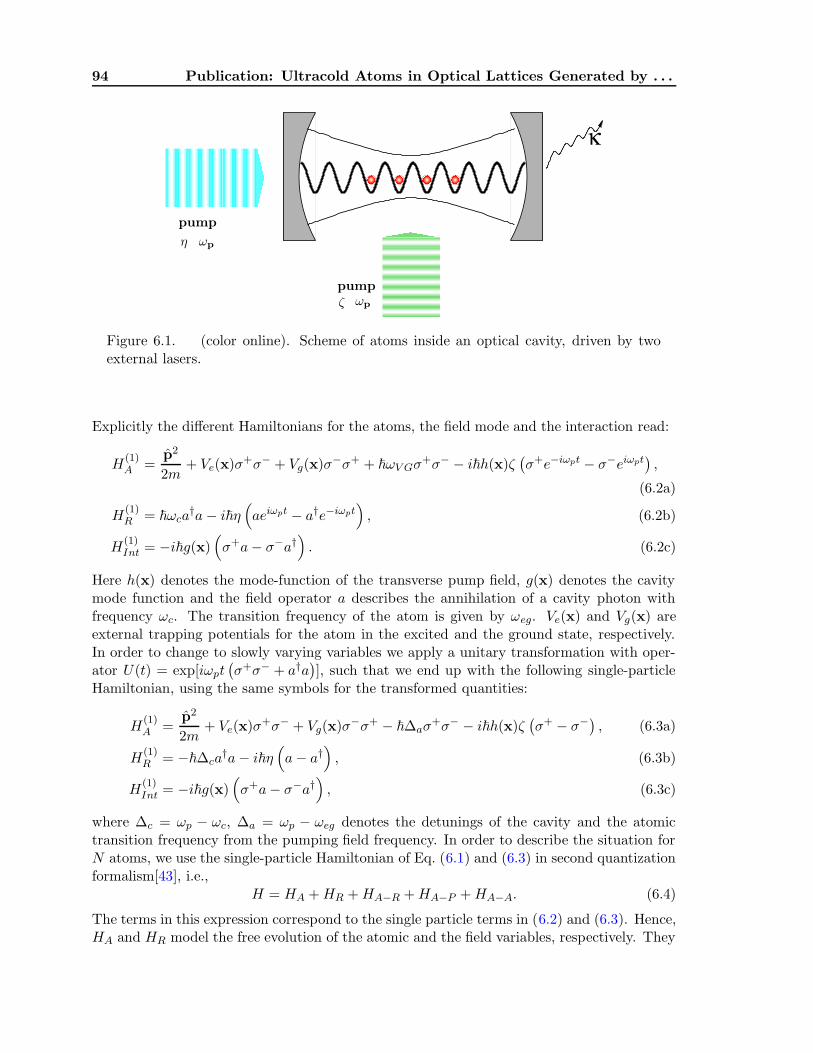
94 Publication: Ultracold Atoms in Optical Lattices Generated by . . .
Figure 6.1. (color online). Scheme of atoms inside an optical cavity, driven by twoexternal lasers.
Explicitly the different Hamiltonians for the atoms, the field mode and the interaction read:
H(1)A =
p2
2m+ Ve(x)σ+σ− + Vg(x)σ−σ+ + ~ωV Gσ
+σ− − i~h(x)ζ(
σ+e−iωpt − σ−eiωpt)
,
(6.2a)
H(1)R = ~ωca
†a− i~η(
aeiωpt − a†e−iωpt)
, (6.2b)
H(1)Int = −i~g(x)
(
σ+a− σ−a†)
. (6.2c)
Here h(x) denotes the mode-function of the transverse pump field, g(x) denotes the cavitymode function and the field operator a describes the annihilation of a cavity photon withfrequency ωc. The transition frequency of the atom is given by ωeg. Ve(x) and Vg(x) areexternal trapping potentials for the atom in the excited and the ground state, respectively.In order to change to slowly varying variables we apply a unitary transformation with oper-ator U(t) = exp[iωpt
(
σ+σ− + a†a)
], such that we end up with the following single-particleHamiltonian, using the same symbols for the transformed quantities:
H(1)A =
p2
2m+ Ve(x)σ+σ− + Vg(x)σ−σ+ − ~∆aσ
+σ− − i~h(x)ζ(
σ+ − σ−)
, (6.3a)
H(1)R = −~∆ca
†a− i~η(
a− a†)
, (6.3b)
H(1)Int = −i~g(x)
(
σ+a− σ−a†)
, (6.3c)
where ∆c = ωp − ωc, ∆a = ωp − ωeg denotes the detunings of the cavity and the atomictransition frequency from the pumping field frequency. In order to describe the situation forN atoms, we use the single-particle Hamiltonian of Eq. (6.1) and (6.3) in second quantizationformalism[43], i.e.,
H = HA +HR +HA−R +HA−P +HA−A. (6.4)
The terms in this expression correspond to the single particle terms in (6.2) and (6.3). Hence,HA and HR model the free evolution of the atomic and the field variables, respectively. They
6.2. Model 95
read as:
HA =
∫
d3x
[
Ψ†g(x)
(
− ~2
2m∇2 + Vg(x)
)
Ψg(x) + Ψ†e(x)
(
− ~2
2m∇2 − ~∆a + Ve(x)
)]
Ψe(x),
(6.5)where Ψg(x) and Ψe(x) denotes the atomic field operators for annihilating an atom at positionx in the ground state and the excited state, respectively. They obey the usual bosoniccommutation relations
[
Ψf (x),Ψ†f ′(x
′)]
= δ3(
x− x′) δf,f ′ (6.6a)[
Ψf (x),Ψf ′(x′)]
=[
Ψ†f (x),Ψ†
f ′(x′)]
= 0, (6.6b)
for f, f ′ ∈ e, g. The field operator remains unchanged, i.e., HR = −~∆ca†a− i~η
(
a− a†)
.The two-body interaction is modeled by a short-range pseudopotential [44], characterized bythe s-wave scattering length as, leading to a Hamiltonian
HA−A =U
2
∫
d3x؆g(x)؆
g(x)Ψg(x)Ψg(x), (6.7)
where U = 4πas~2/m. The coupling of the cavity field with the atoms inside the cavity is
given by
HA−R = −i~∫
d3xΨ†g(x)g(x)aΨe(x) + h.c., (6.8)
whereas the interaction with the laser beam, which coherently drives the atoms, reads
HA−P = −i~ζ∫
d3xΨ†g(x)h(x)Ψe(x) + h.c.. (6.9)
Let us now calculate the Heisenberg equations for the various field operators, startingwith the operator for the excited state, i.e.,
∂Ψe(x)
∂t= i
[
~
2m∇2 − Ve(x)
~+ ∆a
]
Ψe(x)− [g(x) + ζh(x)] Ψg(x). (6.10)
The first term corresponds to the free evolution of the atomic state, whereas the second termdescribes the absorption of a cavity photon or a pump photon together with the annihilationof a ground state atom. Similarly, the equation for the ground state operator reads:
∂Ψg(x)
∂t= i
[
~
2m∇2 − Vg(x)
~− U
~Ψ†g(x)Ψg(x)
]
Ψg(x) + [g(x) + ζh(x)] Ψe(x). (6.11)
Finally, the Heisenberg equation for the cavity field operator is given by:
∂a
∂t= i∆ca+ η +
∫
d3xg(x)Ψ†g(x)Ψe(x). (6.12)
Again, the first term corresponds to the free field evolution, whereas the last two terms aredriving terms of the cavity field.

96 Publication: Ultracold Atoms in Optical Lattices Generated by . . .
As we want to treat temperatures close to T = 0 we have to avoid heating and the modelonly makes sense for very weak atomic excitation, where there is only negligible spontaneousemission. In this limit we can adiabatically eliminate the excited states from the dynamicsof our system. This requires large atom-pump detunings ∆a, where we also can neglect thekinetic energy term and the trapping potential in (6.10) compared to ∆a. Necessarily, weassume that the field operators Ψg(x) and a vary on a much slower time scale than the 1/∆a
terms, such that we obtain:
Ψe(x, t) = − i
∆a[ζh(x) + g(x)a(t)] Ψg(x, t). (6.13)
Inserting this expression for Ψe(x) into (6.11) and (6.12) leads then to:
∂Ψg(x)
∂t= i
[
~
2m∇2 − Vg(x)
~− ζ2h2(x)
∆a− g2(x)
∆aa†a
−ζh(x)g(x)
∆a
(
a+ a†)
− U
~Ψ†g(x)Ψg(x)
]
Ψg(x), (6.14)
∂a
∂t= i
[
∆c −1
∆a
∫
d3xg2(x)Ψ†g(x)Ψg(x)
]
a− iζ
∆a
∫
d3xh(x)Ψ†g(x)Ψg(x) + η. (6.15)
The central trick is now to find an effective Hamiltonian Heff which leads to the samedynamics as given by Eq. (6.14) and (6.15). Thus this Hamiltonian has to obey:
i~∂Ψg(x)
∂t= [Ψg(x),Heff] and i~
∂a
∂t= [a,Heff] . (6.16)
From this we can easily read off a possible effective Hamiltonian of the form:
Heff =
∫
d3x؆g(x)
− ~2
2m∇2 + Vg(x)
+~
∆a
[
ζ2h2(x) + g2(x)a†a+ ζh(x)g(x)(
a+ a†)]
Ψg(x)
+U
2
∫
d3x؆g(x)؆
g(x)Ψg(x)Ψg(x)− i~η(
a− a†)
− ~∆ca†a. (6.17)
The corresponding single particle Hamiltonian, which leads to this second quantized Hamil-tonian is [45]:
H(1)eff =
p2
2m+Vg(x)+
~
∆a
[
ζ2h2(x) + g2(x)a†a+ ζh(x)g(x)(
a+ a†)]
−i~η(
a− a†)
−~∆ca†a.
(6.18)
This simplified effective atom-field Hamiltonian will be the basis of our further consid-erations. It is, however, still much too complex for a general solution and we will have tomake further simplifying assumptions. Hence at this point we will restrict ourselves to 1Dmotion along the cavity axis. In an experimental setup this could be actually realized bya deep radial trapping potential, but we think that at least qualitatively the model shouldalso capture the essential physics if some transverse motion of the particles was allowed. As
6.2. Model 97
one consequence this assumption requires a rescaling of the effective two-body interactionstrength [46], which enters as an open parameter in our model anyway.
Mathematically we thus end up with a one-dimensional optical lattice, wich is partlygenerated by the resonator field and superimposed onto a prescribed extra trapping po-tential Vg(x) = Vg(x). The mode function of the cavity along the axis is approximatedby g(x) = g(x) = g0 cos(kx) and the transverse laser beam forms a broad standing waveh(x) = h0 cos(kpy), which in our one-dimensional considerations (y = 0) is just a constantterm that we can eventually omit in (6.17).
As we consider external pumping of atoms and mode, we essentially treat an open systemand we have to deal with dissipation as well. Such dissipation processes are modeled byLiouvillean terms L appearing in the master equation for the atom-field density operator,i.e.,
% =1
i~[Heff, %] + L%. (6.19)
As mentioned above, we assume large atom-pump detuning ∆a, suppressing spontaneousemission to a large extend. However, we still have to deal with the cavity loss κ, whichwill thus be the dominant dissipation process. Hence the corresponding Liouvillean using astandard quantum optics approach [49] reads:
L% = κ(
2a%a† − a†a%− %a†a)
. (6.20)
Equivalently in the corresponding Heisenberg equation for the field operator, cavity lossleads to damping terms and fluctuations, so that it then reads:
a =
i
[
∆c −g20
∆a
∫
dxΨ†g(x) cos2(kx)Ψg(x)
]
− κ
a
− iζg0h0
∆a
∫
dxΨ†g(x) cos(kx)Ψg(x) + η + Γin. (6.21)
Since we will be mainly interested in normally ordered quantities and assume vacuum (T=0)outside the cavity, the input noise operators Γin will not enter in the dynamics, such that wewill omit them later.
Let us proceed and transform the Hamiltonian in a more commonly known form. Follow-ing standard procedures, one constructs maximally localized eigenfunctions at each site andexpands the atomic field operator Ψg(x) in terms of single atom Wannier functions [48]
Ψg(x) =∑
n
∑
k
bn,kwn(x− xk), (6.22)
where bn,k corresponds to the annihilation of a particle in the n−th energy band at site k.Since we assume the involved energies to be much smaller than the excitation energies to thesecond band, we are able to keep only the lowest vibrational state in the Wannier expansion,i.e., Ψg(x) =
∑
k bkw(x−xk), where w(x) = w0(x). This yields to the following Hamiltonian:
H =∑
k,l
Eklb†kbl +
(
~U0a†a+ Vcl
)
∑
k,l
Jklb†kbl + ~ηeff
(
a+ a†)
∑
k,l
Jklb†kbl − i~η
(
a− a†)
+1
2
∑
i,j,k,l
Uijklb†i b
†jbkbl − ~∆ca
†a, (6.23)

98 Publication: Ultracold Atoms in Optical Lattices Generated by . . .
where the addendum eff of the Hamiltonian is omitted. Here we introduced an importantcharacteristic parameter of atomic cavity QED, namely the refractive index U0 of a singleatom at an antinode, which is given by U0 = g2
0/∆a. It gives the frequency shift of the cavitymode induced by a single atom at an antinode and also corresponds to the optical latticedepth for an atom per cavity photon [17]. Similarly, the parameter ηeff = g0h0ζ/∆a describesthe position dependent effective pump strength of the cavity mode induced by the scatteredlight from a single atom at an antinode.
Note that in contrast to a free space lattice the Wannier state expansion, Eq. 6.22 is arather formal procedure here, as the potential depth and thus the Wannier functions dependon the cavity field and thus in principle are dynamic quantities, which have to be determinedconsistently. This is of course consequently also true for the various coupling parametersin the Hamiltonian. The above model thus can only be valid as long as the single bandapproximation stays valid during the system dynamics. In particular in the case, where theatoms are trapped solely by the cavity field [21, 22] this is not valid for very low photonnumbers.
In principle this problem can be circumvented by adding an additional external trappingpotential Vg(x) to the model, which guarantees a minimum potential depth even in the case ofzero cavity photons. Practically this is feasible, for instance, with a far detuned, off-resonantdipole trap (FORT) [50], i.e., Vg(x) = Vcl cos
2(kFx), where kF denotes the wave number of theFORT field. In the experimental realization, the frequency of the corresponding laser field ωFis only very few free spectral ranges separated from the main cavity frequency ωc [27, 51, 52].Hence, in the vicinity of the cavity center, the coincidence of the FORT field and the cavityfield is very good, and we can replace in good agreement cos2(kFx) with cos2(kx).
Let us remark here that by including this extra potential we have saved our model andallowed for further analytical analysis of the dynamics, but we also have thrown out a greatdeal of interesting physics already. Actually, for very few atoms one still can solve the fullHamiltonian without the restriction to the lowest bands by quantum Monte Carlo wave-function simulations. Some early results of such simulations can be found in Ref. [55, 56].However, this is not the subject of this work and we will proceed here with the effectivelattice model under the assumption of a deep enough extra potential or strong enough cavityfields.
Note that in (6.23), in contrast to the case of the Bose-Hubbard model in a classical opticallattice, where the matrix elements of the potential and kinetic energy can be merged, heretwo separate parts exist due to the presence of the cavity field operators in the Hamiltonian.Explicitly they read as:
Ekl =
∫
dxw(x− xk)(
− ~2
2m∇2
)
w(x− xl), (6.24a)
Jkl =
∫
dxw(x− xk) cos2(kx)w(x − xl), (6.24b)
Jkl =
∫
dxw(x− xk) cos(kx)w(x − xl). (6.24c)
The on-site elements Jkk and Ekk are independent of the lattice site k, whereas Jkl changessign periodically, i.e., Jkk = −Jk+1,k+1 due to the cos, which has twice the periodicity of
6.3. Cavity pump 99
the lattice. This also accounts for Jk,k+1 = 0. Note that the existence of this term impliesthat two adjacent wells acquire different depths forcing us to reassure that for the case ofthe directly pumped atom ηeff(a+ a†) cos(kx) is only a small perturbation of the lattice. Asthe next-nearest elements are typically two orders of magnitude smaller than the nearest-neighbor term [3] they can safely be neglected (tight-binding approximation). Furthermore,in the case of the nonlinear interaction matrix elements,
Uijkl = g1D
∫
dxw(x− xi)w(x− xj)w(x − xk)w(x − xl) (6.25)
we can omit the off-site terms since they are also typically two orders of magnitude smallerthan the on-site interaction matrix elements. Note that g1D is the one-dimensional on-siteinteraction strength, originating from an adjustment of the scattering length as, due to thetransversal trapping [46]. As a central result of our studies we therefore obtain a generalizedBose-Hubbard Hamiltonian:
H = E0N +EB +(
~U0a†a+ Vcl
)(
J0N + JB)
+ ~ηeff
(
a+ a†)
J0
∑
k
(−1)k+1nk
− ~∆ca†a− i~η
(
a− a†)
+U
2
∑
k
nk (nk − 1) , (6.26)
where the nonlinear on-site interaction is characterized by U = 4πas~2
m
∫
dx |w(x)|4 . In ad-
dition, we introduced the number operator N =∑
k nk =∑
k b†kbk and the jump operator
B =∑
k
(
b†k+1bk + h.c.)
. The site-independent on-site matrix elements are labeled E0, J0
and J0, whereas E and J are the site-to-site hopping elements. Note that for strong classicalintracavity fields and no transverse pump we recover the standard Bose-Hubbard Hamilto-nian.
Finally, let us remark that we now can also rewrite the field Heisenberg Eq. (6.21) in theabove terms, which gives:
a =
i[
∆c − U0
(
J0N + JB)]
− κ
a+ η − iηeffJ0
∑
k
(−1)k+1nk. (6.27)
Here we clearly see that besides the number operator N for the atoms also the coherenceproperties via the operator B and statistics via nk plays a decisive role in the field dynamics.As this field acts back on the atomic motion, interesting and complex coupled dynamicscan be expected from this model, which was partly already discussed in [32, 33] and will beelucidated more in the remainder of this work.
6.3 Cavity pump
Let us now turn to the conceptually simplest case and restrict the pumping only to the cavity,where a only single mode is coherently excited (cavity pumping). This mode will generate anoptical potential in addition to the prescribed external potential. For large enough photonnumbers the external potential can be even omitted and the particles are trapped solely by

100 Publication: Ultracold Atoms in Optical Lattices Generated by . . .
the cavity field. As essential ingredient in the dynamics, the identical coupling of all atomsto this same field mode induces a long-range interaction between the atoms independent oftheir positions. Setting ηeff = 0, the Hamiltonian (6.26) is reduces to:
H = E0N +EB +(
~U0a†a+ Vcl
)(
J0N + JB)
− ~∆ca†a− i~η
(
a− a†)
+U
2C. (6.28)
Here we introduced C =∑
k nk (nk − 1) for the operator of the two-body on-site interaction.Still we see that the corresponding Heisenberg equation for the cavity field:
a =
i[
∆c − U0
(
J0N + JB)]
− κ
a+ η. (6.29)
depends on photon number and coherence. For very weak fields this yields an atom statisticsdependent cavity transmission spectrum, which was studied in some detail in Ref. [35]. Herewe go one step further and study the dynamical back action of the field onto atomic motionand field mediated atom-atom interaction, which appear at higher photon number. As themodel is still rather complex we need some further approximations at this point in order tocatch some qualitative insight.
6.3.1 Field-eliminated Hamiltonian
Although the influence of the cavity field on the atoms is equal on all particles, their commoninteraction generates a dynamics much more complex than for a Bose-Hubbard model withprescribed external potential. This is more analogous to real solid state physics where thestate of the electrons also acts back on the potentials. To exhibit the underlying physics,we will now derive an approximate Hamiltonian, which solely depends on particle variablesby adiabatically eliminating the field (6.28). This should be valid when the damping rateκ of the cavity generates a faster time scale than the external atomic degrees of freedom.Actually as tunneling is mostly a very slow process (much slower than the recoil frequency),this will be almost always the case in practical experimental setups. To this end, we simplyequate (6.29) to zero and obtain formally a = η/κ− i[∆c−U0(J0N+JB)]. In the followingwe constrain ourselves to the case of a fixed number of atoms, i.e., N = N1. The very smalltunneling matrix element J can be used as an expansion parameter, leading to:
a ≈ η
κ− i∆′c
[
1− i U0J
κ− i∆′c
B − (U0J)2
(κ− i∆′c)
2B2
]
, (6.30)
where we introduced a shifted detuning ∆′c = ∆c − U0N .
In order to obtain an effective Hamiltonian, where the cavity degrees of freedom areeliminated, we replace the field terms in (6.28), by the steady state expressions (6.30), as wellas in the Liouville super operator (6.20). Note, that this is more appropriate than the naiveapproach of a replacement just in the Hamiltonian, as has been done in our former work [32].If we consider terms up to order ∝ J 2, the exchange in the Hamiltonian yields:
Had = (E + JVcl)B +U
2C +
~U0Jη2
κ2 + ∆′c2
(
∆′c2 − κ2
κ2 + ∆′c2 B −
3U0J∆′c
κ2 + ∆′c2 B
2
)
. (6.31)

6.3. Cavity pump 101
Next, we apply the same procedure to the Liouville equation - again up to terms ∝ J 2 - weobtain an adiabatic Liouville operator:
Lad% = −i 2U0Jκ2η2
(
κ2 + ∆′c2)2
[
B +2∆′
cU0J
κ2 + ∆′c2 B
2, %
]
+κU2
0 J2η2
(
κ2 + ∆′c2)2
(
2B%B − B2%− %B2)
. (6.32)
The Lindblad terms in the second line are real, corresponding to dissipation, whereas thefirst, imaginary term corresponds to a unitary time evolution and has therefore to be addedto the adiabatic Hamiltonian, i.e.,
Had → Had +2~U0Jκ
2η2
(
κ2 + ∆′c2)2
(
B +2∆′
cU0J
κ2 + ∆′c2 B
2
)
.
Altogether, we end up with a Hamiltonian, where the cavity field has been eliminated:
Had = (E + JVcl)B +U
2C +
~U0Jη2
κ2 + ∆′c2
(
B +U0J∆′
c
κ2 + ∆′c2
κ2 − 3∆′c2
κ2 + ∆′c2 B
2
)
. (6.33)
The loss rate of the cavity is described by the remaining dissipative part of (6.32):
Lad% =κU2
0 J2η2
(
κ2 + ∆′c2)2
(
2B%B − B2%− %B2)
. (6.34)
Note, that the above adiabatic elimination procedure is not completely unambiguous dueto ordering freedom. Nevertheless it should give a qualitatively correct first insight. Analternative way of deriving an effective Hamiltonian, depending solely on particle observableis similar to (6.16) and (6.17). This amounts to a replacement of the field variables with (6.30)in the Heisenberg equation for the external atomic degrees of freedom, which read as follows:
bk =1
i~
[(
E + JVcl + ~U0Ja†a)
(bk−1 + bk+1)− Unkbk]
. (6.35)
A naive replacement of the field operator a and its adjoint a† by (6.30) in the above expressionleads to an equation for bk, which cannot be generated from an effective adiabatic Hamiltonianin the form bk = −i/~[bk,Had]. Hence, before substituting the adiabatic field operators, wehave to symmetrize the expression containing the field term in (6.35) in the form
bk = − i~
[(E + JVcl) (bk−1 + bk+1)− Unkbk]−i~U0J
2
[
a†a (bk−1 + bk+1) + (bk−1 + bk+1) a†a]
.
(6.36)This form enables us to describe the dynamics of bk by a Heisenberg equation with an effectiveHamiltonian, which up to second order in J reads:
Had = (E + JVcl)B +U
2C +
~U0Jη2
κ2 + ∆′c2
(
B +U0J∆′
c
κ2 + ∆′c2 B
2
)
. (6.37)
The terms in the second line stem from the field terms in (6.36). Although this Hamiltonianlooks a bit different from the first version derived before (6.33), their properties are - within

102 Publication: Ultracold Atoms in Optical Lattices Generated by . . .
their regime of validity - in very good agreement as long as hopping is slow compared todamping.
To exhibit the physical content of this Hamiltonian one can look at its eigenstates. Asfirst step we calculate the Mott insulator state [see Eq. (6.49)] fraction of the lowest energystate |ψ〉 of these two Hamiltonians, i.e., pMI = |〈ψ|MI〉|2 (see also Fig. 6.4), as a function ofthe on-site interaction energy for different values of ∆′
c. This will indicate changes of positionand behavior of the Mott insulator superfluid transition. as shown in Fig. 6.4. To comparethe two approximate Hamiltonians in Fig. 6.2, we plot the difference of the Mott insulatorfraction of the ground state of (6.33) and (6.37), as well as the difference of the steady statephoton number. Obviously the two Hamiltonians, converge in the limit of large cavity decayκ. This can also be seen in Fig. 6.2, where the dashed-dotted line depicts the case of a smaller∆′c (which is equivalent to an enlarged κ), showing a strongly enhanced coincidence.
6.3.2 Field-eliminated density operator
Let us now use a further and somehow more systematic alternative approach to eliminatethe cavity field dynamics from the system evolution directly from the Liouville equation byfollowing a method proposed by Wiseman and Milburn [53], which is valid for large κ andlow photon numbers. In this case we have
∣
∣
∣
∣
〈Hat〉κ
∣
∣
∣
∣
∼∣
∣
∣
∣
~U0〈a†a〉κ
∣
∣
∣
∣
= ε 1, (6.38)
where Hat is the atomic part of (6.28), i.e., Hat = (E + VclJ) B + UC/2. Again the totalatom number N is supposed to be constant. This allows to expand the density operator inpowers of ε, corresponding to states with increasing photon number:
% = %0 ⊗ |0〉a〈0|+ (%1 ⊗ |1〉a〈0|+ h.c.) + %2 ⊗ |1〉a〈1|+(
%′2 ⊗ |2〉a〈0|+ h.c.)
+O(
ε3)
. (6.39)
Here %i are density operators for the particle variables, corresponding to the order i of mag-nitude in the expansion parameter ε. We substitute this expression into the Liouville equa-tion (6.19) with the Hamiltonian from (6.28), which leads to the following set of equations:
%0 =1
i~[Hat, %0]− η
(
%1 + %†1
)
+ 2κ%2 (6.40a)
%1 =1
i~[Hat, %1]− η
(√2%′2 + %2 − %0
)
− κ%1 (6.40b)
+ i[
∆c − U0
(
J0N + JB)]
%1 + κO(
ε4)
%2 =1
i~[Hat, %2] + η
(
%1 + %†1
)
− 2κ%2 − iU0
[
J0N + JB, %2
]
+ κO(
ε4)
(6.40c)
%′2 =1
i~
[
Hat, %′2
]
+√
2η%1 − 2κ%′2 + 2i[
∆c − U0
(
J0N + JB)]
%′2 + κO(
ε4)
,(6.40d)
Now we adiabatically eliminate the off-diagonal elements %1 and %′2. Setting their derivationsin (6.40b) and (6.40d) to zero and neglecting terms with respect to the assumption (6.38),we obtain:
%′2 =η√2A
%1 +O(
ε3)
. (6.41)
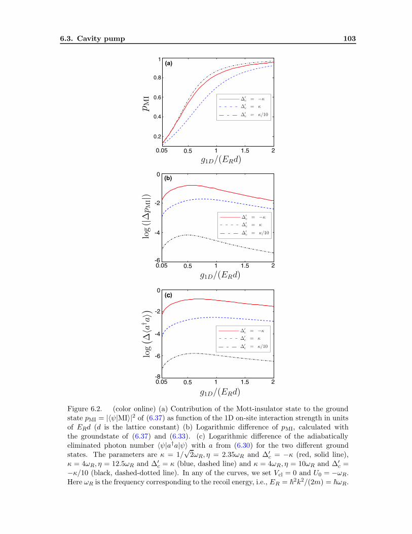
6.3. Cavity pump 103
Figure 6.2. (color online) (a) Contribution of the Mott-insulator state to the groundstate pMI = |〈ψ|MI〉|2 of (6.37) as function of the 1D on-site interaction strength in unitsof ERd (d is the lattice constant) (b) Logarithmic difference of pMI, calculated withthe groundstate of (6.37) and (6.33). (c) Logarithmic difference of the adiabaticallyeliminated photon number 〈ψ|a†a|ψ〉 with a from (6.30) for the two different groundstates. The parameters are κ = 1/
√2ωR, η = 2.35ωR and ∆′
c = −κ (red, solid line),κ = 4ωR, η = 12.5ωR and ∆′
c = κ (blue, dashed line) and κ = 4ωR, η = 10ωR and ∆′c =
−κ/10 (black, dashed-dotted line). In any of the curves, we set Vcl = 0 and U0 = −ωR.Here ωR is the frequency corresponding to the recoil energy, i.e., ER = ~
2k2/(2m) = ~ωR.
104 Publication: Ultracold Atoms in Optical Lattices Generated by . . .
This is consistent with the assumption %′2 ∼ O(
ε2)
. Here we defined A = κ− i∆′c + iU0JB.
Putting (6.41) into (6.40b) and neglecting the terms consistent with the order of the expan-sion, such that %1 ∼ O (ε), it follows that:
%1 =η
A+ η2/A(%0 − %2) +O
(
ε4)
. (6.42)
We simplify this expression, %1 ≈ ηA−1(%0−%2), which is consistent with the above expansionand substitute it into (6.40a) and (6.40c):
%0 =1
i~[Hat, %0] + 2κ%2 − η2
[
A−1 (%0 − %2) + (%0 − %2)A†−1]
(6.43a)
%2 =1
i~[Hat, %2]− iU0
[
J0N + JB, %2
]
− 2κ%2
+ η2[
A−1 (%0 − %2) + (%0 − %2)A†−1]
. (6.43b)
In order to formulate a master equation for the particle variables we have to use the reduceddensity operator, where we trace over the field variables, i.e., %at = tr(%) = %0 + %2 +O
(
ε4)
.With (6.43a) and (6.43b) we see that:
%at =1
i~[Hat, %at]− iU0
[
J0N + JB, %2
]
. (6.44)
As a further approximation, which is also consistent with the expansion order of the assump-tion (6.38), we set (6.43b) to zero and neglect [Hat, %2] and all other terms smaller thanO(
ε3)
. Then we can express %2 through %0:
%2 =η2
2κ
[
A−1%0 + %0A†−1]
. (6.45)
Within this order of magnitude of ε we can replace %0 with %at, leading us finally to thefollowing master equation for the reduced density operator of the particle variables:
%at =1
i~[Hat, %at]− i
U0η2
2κ
[
J0N + JB,(
A−1%at + %atA†−1)]
. (6.46)
Note that this model also contains a damping part, since the operator A is not hermitian.Let us investigate this damping, by expanding the inverse of A up to first order in J , whichis consistent with the order of magnitude in (6.46). Hence we replace A−1 and its adjoint inthis equation by
A−1 ≈ 1
κ− i∆′c
(
1− i U0J
κ− i∆′c
B
)
(6.47)
and its adjoint. Since we are restricted on a subspace of constant atom number, the Liouvilleequation reads as follows:
%at =1
i~
[
Hat +~U0η
2
κ2 + ∆′c2
(
JB +U0∆
′cJ
2
κ2 + ∆′c2 B
2
)
, %at
]
− (JU0η)2
2κ
κ2 −∆′c2
(
κ2 + ∆′c2)2
[
B,[
B, %at
]]
.
(6.48)Obviously, the non-dissipative part of this equation agrees perfect with our adiabaticallyeliminated Hamiltonian (6.37) and the structure of the dissipative part is of the same Lindbladform as (6.34). Note that an expansion of A−1 to higher order in J would also provide us thecorrect next-order term of (6.37) plus an extra term in the Liouville-equation, which doesnot correspond to unitary time evolution, as described by a Hamiltonian. This confirms theusefulness of the naive elimination method, also used in Ref. [32]

6.3. Cavity pump 105
6.3.3 Quantum phase transitions in an optical lattice
In section 6.3.1 we derived two approximate Hamiltonians (6.33) and (6.37) describing oursystem of cold atoms in an optical lattice. To a large extend they still implement the wellknown BH model, but with parameters controllable via cavity detuning and some additionalnonlocal interaction terms. Let us now investigate their properties in some more detail. Oneof the key features of optical cavities is the feedback mechanism between atoms and cavityfield. Hence, computations are a subtle issue, since the matrix elements in the BH Hamilto-nian depend on the field amplitude, which itself depends on the atomic positions. In principlea rigorous treatment would consist of calculating the matrix elements (6.24) for every photonFock state and treating the parameters of the BH model as operators. To avoid the fullcomplexity of such an approach we will first assume only a weak dependence of the Wannierfunctions on the mean cavity photon number 〈a†a〉, which allows us to proceed analytically.For any set of operating parameters we then calculated the matrix elements in a self-consistentway replacing the photon number operator by its average in the iteration process. Explicitly
this is implemented by starting from some initial guess J(0)0 , E
(0)0 , J (0), E(0) in the Hamilto-
nian (6.37), from which we calculate the ground state |ψ(0)〉. By use of this state we obtain aninitial mean photon number 〈ψ(0)|a†a|ψ(0)〉, with the steady-state field operator (6.30). Now
we can calculate the matrix elements J(1)0 , E
(1)0 , J (1), E(1) again leading to a new ground state
|ψ(1)〉 and a new mean photon number 〈ψ(1)|a†a|ψ(1)〉. Proceeding iteratively, in most casethe fixpoint is reached already after very few iterations and the system properties are thencalculated with this self-consistent matrix elements. The convergence speed decreases nearthe resonance for the cavity photon number (cf. Fig. 6.3), which occurs for ∆c = U0J0N −κ,especially for large U0. Introducing some damping in the iteration procedure easily resolvesthis issue, though. As we mentioned already before, we restrict the model on a subspace HN
Figure 6.3. (color online). Self-consistent photon number in the case of four particlesin four wells without on-site interaction. Parameters are U0 = −ωR and κ = ωR.
of a fixed total particle number N in an optical lattice of M sites. A basis of HN consistsof the states |N, 0, 0, . . . , 0〉, |N − 1, 1, 0, . . . , 0〉, . . . , |0, 0, . . . , 0, N〉. Since we are interested in
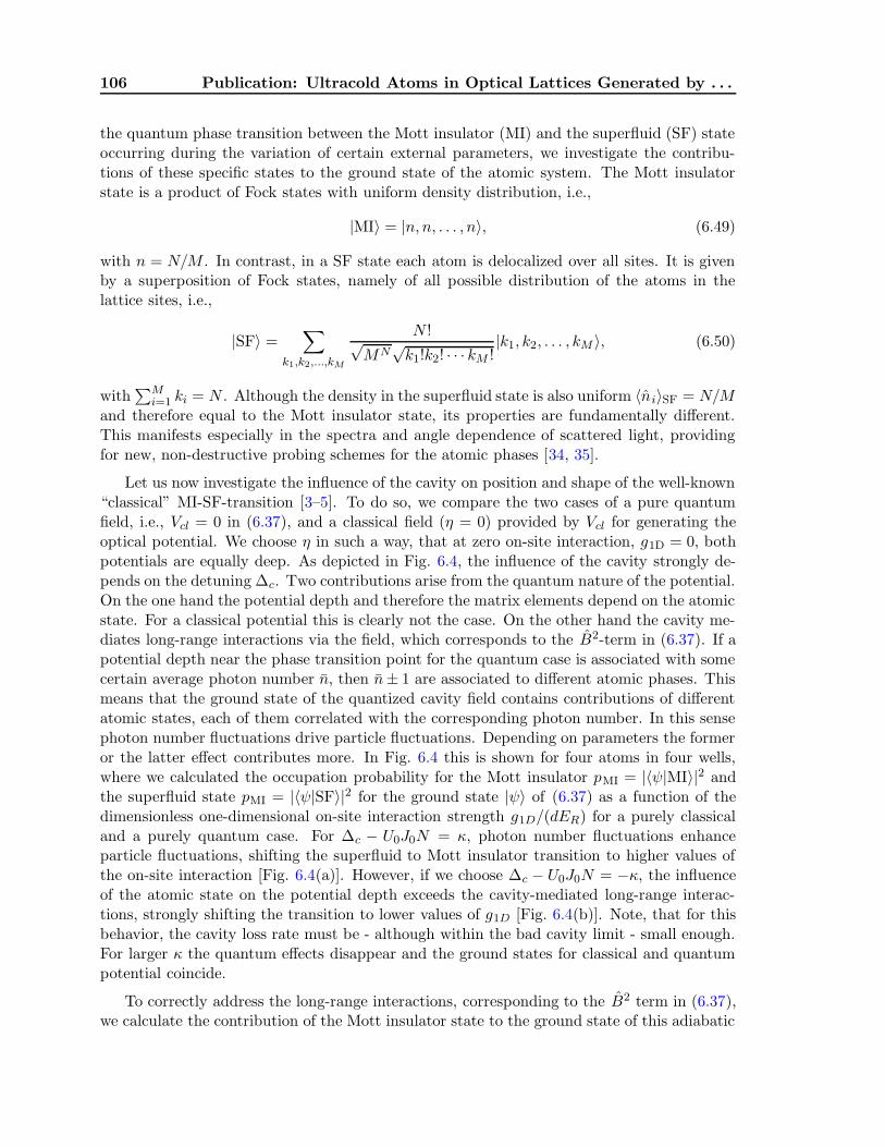
106 Publication: Ultracold Atoms in Optical Lattices Generated by . . .
the quantum phase transition between the Mott insulator (MI) and the superfluid (SF) stateoccurring during the variation of certain external parameters, we investigate the contribu-tions of these specific states to the ground state of the atomic system. The Mott insulatorstate is a product of Fock states with uniform density distribution, i.e.,
|MI〉 = |n, n, . . . , n〉, (6.49)
with n = N/M . In contrast, in a SF state each atom is delocalized over all sites. It is givenby a superposition of Fock states, namely of all possible distribution of the atoms in thelattice sites, i.e.,
|SF〉 =∑
k1,k2,...,kM
N !√MN√k1!k2! · · · kM !
|k1, k2, . . . , kM 〉, (6.50)
with∑M
i=1 ki = N . Although the density in the superfluid state is also uniform 〈ni〉SF = N/Mand therefore equal to the Mott insulator state, its properties are fundamentally different.This manifests especially in the spectra and angle dependence of scattered light, providingfor new, non-destructive probing schemes for the atomic phases [34, 35].
Let us now investigate the influence of the cavity on position and shape of the well-known“classical” MI-SF-transition [3–5]. To do so, we compare the two cases of a pure quantumfield, i.e., Vcl = 0 in (6.37), and a classical field (η = 0) provided by Vcl for generating theoptical potential. We choose η in such a way, that at zero on-site interaction, g1D = 0, bothpotentials are equally deep. As depicted in Fig. 6.4, the influence of the cavity strongly de-pends on the detuning ∆c. Two contributions arise from the quantum nature of the potential.On the one hand the potential depth and therefore the matrix elements depend on the atomicstate. For a classical potential this is clearly not the case. On the other hand the cavity me-diates long-range interactions via the field, which corresponds to the B2-term in (6.37). If apotential depth near the phase transition point for the quantum case is associated with somecertain average photon number n, then n± 1 are associated to different atomic phases. Thismeans that the ground state of the quantized cavity field contains contributions of differentatomic states, each of them correlated with the corresponding photon number. In this sensephoton number fluctuations drive particle fluctuations. Depending on parameters the formeror the latter effect contributes more. In Fig. 6.4 this is shown for four atoms in four wells,where we calculated the occupation probability for the Mott insulator pMI = |〈ψ|MI〉|2 andthe superfluid state pMI = |〈ψ|SF〉|2 for the ground state |ψ〉 of (6.37) as a function of thedimensionless one-dimensional on-site interaction strength g1D/(dER) for a purely classicaland a purely quantum case. For ∆c − U0J0N = κ, photon number fluctuations enhanceparticle fluctuations, shifting the superfluid to Mott insulator transition to higher values ofthe on-site interaction [Fig. 6.4(a)]. However, if we choose ∆c − U0J0N = −κ, the influenceof the atomic state on the potential depth exceeds the cavity-mediated long-range interac-tions, strongly shifting the transition to lower values of g1D [Fig. 6.4(b)]. Note, that for thisbehavior, the cavity loss rate must be - although within the bad cavity limit - small enough.For larger κ the quantum effects disappear and the ground states for classical and quantumpotential coincide.
To correctly address the long-range interactions, corresponding to the B2 term in (6.37),we calculate the contribution of the Mott insulator state to the ground state of this adiabatic

6.3. Cavity pump 107
Figure 6.4. (color online) Cavity influence of the Mott insulator to superfluid transitionby means of a comparison of the occupation probabilities pMI and pSF for a purelyquantum field, i.e., Vcl = 0, and a purely classical field, i.e., η = 0, as a function ofthe dimensionless one-dimensional on-site interaction strength g1D/(dER). We choose ηsuch that both potentials are of equivalent depth for zero on-site interaction (g1D = 0).The quantum and classical case is depicted with solid and dashed lines, respectively. In(a) we set (U0, κ, η) = (−1, 1/
√2,√
5.5)ωR and ∆c − U0J0N = κ. (b) The same as (a)but with ∆c − U0J0N = −κ.
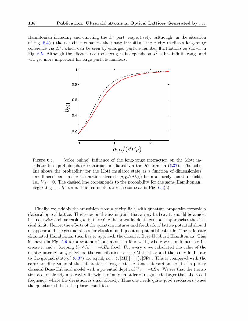
108 Publication: Ultracold Atoms in Optical Lattices Generated by . . .
Hamiltonian including and omitting the B2 part, respectively. Although, in the situationof Fig. 6.4(a) the net effect enhances the phase transition, the cavity mediates long-rangecoherence via B2, which can be seen by enlarged particle number fluctuations as shown inFig. 6.5. Although the effect is not too strong as it depends on J 2 is has infinite range andwill get more important for large particle numbers.
Figure 6.5. (color online) Influence of the long-range interaction on the Mott in-sulator to superfluid phase transition, mediated via the B2 term in (6.37). The solidline shows the probability for the Mott insulator state as a function of dimensionlessone-dimensional on-site interaction strength g1D/(dER) for a a purely quantum field,i.e., Vcl = 0. The dashed line corresponds to the probability for the same Hamiltonian,neglecting the B2 term. The parameters are the same as in Fig. 6.4(a).
Finally, we exhibit the transition from a cavity field with quantum properties towards aclassical optical lattice. This relies on the assumption that a very bad cavity should be almostlike no cavity and increasing κ, but keeping the potential depth constant, approaches the clas-sical limit. Hence, the effects of the quantum natures and feedback of lattice potential shoulddisappear and the ground states for classical and quantum potential coincide. The adiabaticeliminated Hamiltonian then has to approach the classical Bose-Hubbard Hamiltonian. Thisis shown in Fig. 6.6 for a system of four atoms in four wells, where we simultaneously in-crease κ and η, keeping U0η
2/κ2 = −6ER fixed. For every κ we calculated the value of theon-site interaction g1D, where the contributions of the Mott state and the superfluid stateto the ground state of (6.37) are equal, i.e., |〈ψ|MI〉| = |〈ψ|SF〉|. This is compared with thecorresponding value of the interaction strength at the same intersection point of a purelyclassical Bose-Hubbard model with a potential depth of Vcl = −6ER. We see that the transi-tion occurs already at a cavity linewidth of only an order of magnitude larger than the recoilfrequency, where the deviation is small already. Thus one needs quite good resonators to seethe quantum shift in the phase transition.
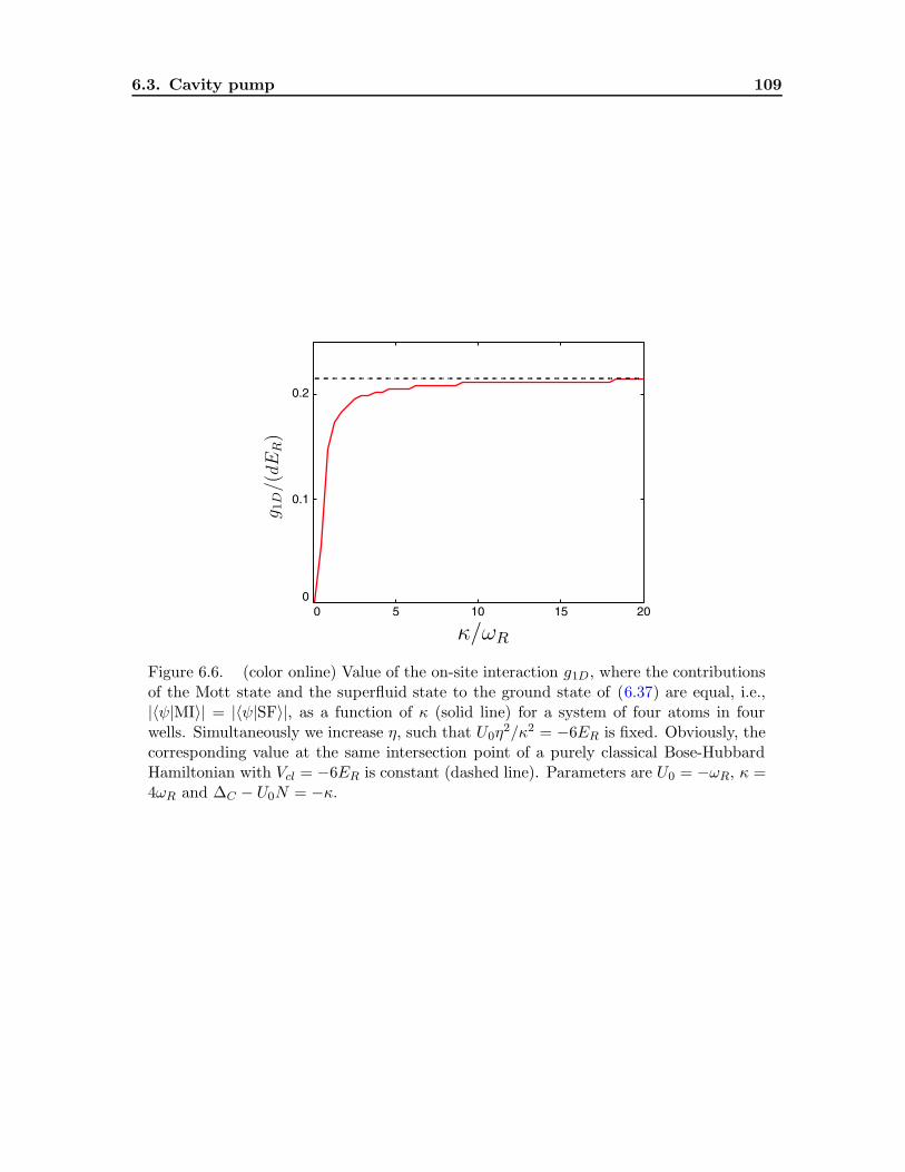
6.3. Cavity pump 109
Figure 6.6. (color online) Value of the on-site interaction g1D, where the contributionsof the Mott state and the superfluid state to the ground state of (6.37) are equal, i.e.,|〈ψ|MI〉| = |〈ψ|SF〉|, as a function of κ (solid line) for a system of four atoms in fourwells. Simultaneously we increase η, such that U0η
2/κ2 = −6ER is fixed. Obviously, thecorresponding value at the same intersection point of a purely classical Bose-HubbardHamiltonian with Vcl = −6ER is constant (dashed line). Parameters are U0 = −ωR, κ =4ωR and ∆C − U0N = −κ.
110 Publication: Ultracold Atoms in Optical Lattices Generated by . . .
6.3.4 Comparison with the full dynamics of the master equation
Using the approximate adiabatic model with eliminated field we have found importantchanges in the physics so far. Even stronger effects are to be expected in the limit of lessand less cavity damping and stronger atom field coupling. Let us now investigate some firstsigns of this and test the range of validity of the above model in this limit. To do so wehave to resort to numerics and compare solutions of the full master equation (6.19) with theground states of the adiabatically eliminated Hamiltonian (6.37). Obviously solving the fullmaster equation is a numerically demanding task. Nevertheless, constraining to few atomsin few wells we are able to solve the equations and reveal the essential physical mechanisms.The limit of the band model description is of course reached for atoms coupled strongly to acavity field with only very few photons and no additional classical potential Vcl present. Herevery strong changes in the tunneling amplitudes occur whenever a photon leaks out of thecavity and reduces the momentary potential depth. This leads to strongly enhanced particlehopping. For instance, one can think of the situations “one photon present” and “no photonpresent”, where the atoms can freely move within the cavity in the absence of an externaltrap. On the other hand one extra photon can almost block hopping. Note that in this casethe ground state atomic configuration can be close to superfluid for a low photon numberand close to an insulator state for a higher photon number. As our matrix elements dependonly on the mean photon number 〈a†a〉, these differences cannot be taken into account in anadiabatic model.
We can explicitly show this behavior by reducing the coupling strength U0, but keepingthe average potential depth fixed (equal matrix elements), by means of a higher averagecavity photon number, which leads to strongly reduced photon number fluctuations. Thisis depicted in Fig. 6.7, where we show the tunneling behavior 〈kx(t)〉 of a single atom ina two well approximation. The atomic ground state of this system is the symmetric state|ψ0〉 = (|l〉+ |r〉) /
√2 having a mean position of 〈kx〉ψ0
= π/2. Here, |l〉 (|r〉) means the left(right) of the two wells. Decreasing U0, increasing η and adjusting ∆c, yields different meanphoton numbers 〈a†a〉, but equal average lattice potential depth V = U0〈a†a〉. (We do notconsider an additional classical potential here.) If only few photons are present, we observelarge fluctuations of the field and the system damps fast to the ground state. As the photonnumber increases, the potential approximates a classical potential as expected, where thereis no dephasing. The (nearly) equal oscillation frequencies show that the matrix elementscoincide for the different photon numbers. This is an interesting feature corresponding to thequantum nature of the potential. In contrast to the Bose-Hubbard model for a classical opticallattice, lattice depth and interaction strength are not the only important system parameters.Quantum fluctuations of the potential are an additional source of atomic fluctuations, playingan essential role in the evolution of the system. Obviously, if only an external potentialis present and the atom is no longer coupled to the cavity field (U0 = 0), the system isundamped, due to the lack of the only dissipation channel present, cavity loss. In this casethe Hamiltonian (6.28) reduces to H = (E + JVcl)B + U/2C, and the atom, initially not inthe symmetric state, oscillates between the left and right well. Note that a more rigoroustreatment of operator-valued matrix elements - as described in the previous section - wouldbe capable of describing this behavior correctly. Alternatively for few atoms Monte-Carlowave function simulations of the full Hamiltonian could be performed, allowing for processes,where the particle leaves the lowest band [54].
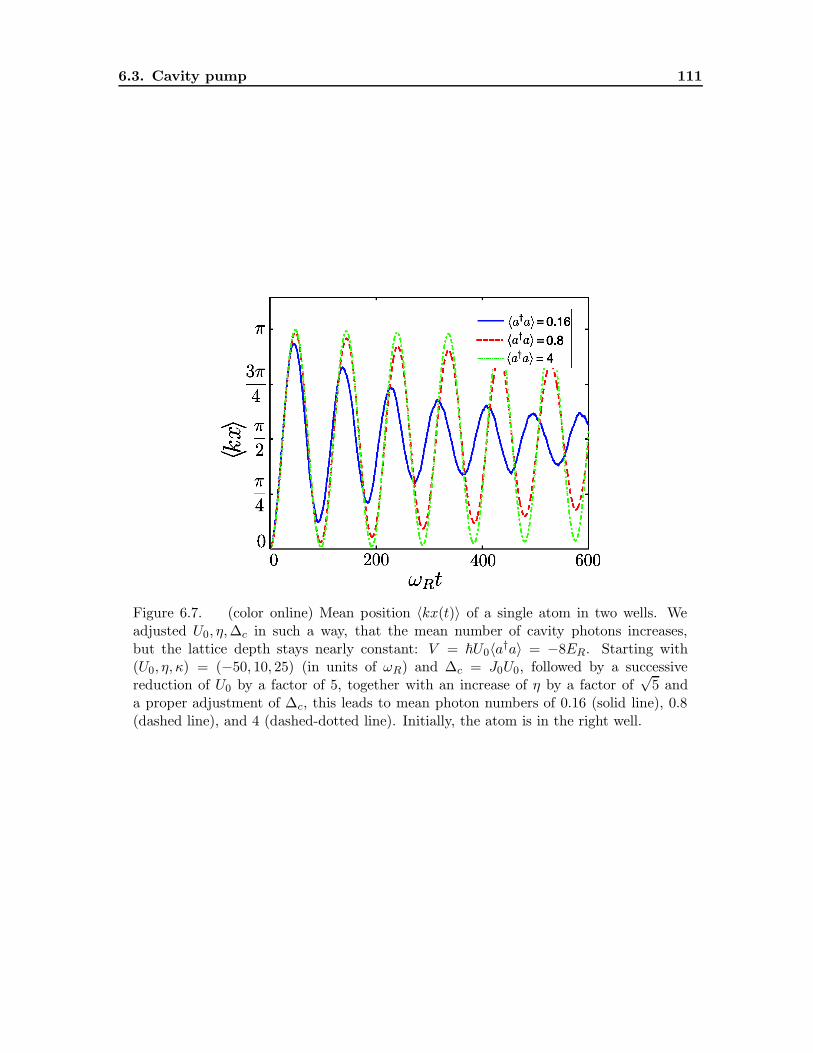
6.3. Cavity pump 111
Figure 6.7. (color online) Mean position 〈kx(t)〉 of a single atom in two wells. Weadjusted U0, η,∆c in such a way, that the mean number of cavity photons increases,but the lattice depth stays nearly constant: V = ~U0〈a†a〉 = −8ER. Starting with(U0, η, κ) = (−50, 10, 25) (in units of ωR) and ∆c = J0U0, followed by a successivereduction of U0 by a factor of 5, together with an increase of η by a factor of
√5 and
a proper adjustment of ∆c, this leads to mean photon numbers of 0.16 (solid line), 0.8(dashed line), and 4 (dashed-dotted line). Initially, the atom is in the right well.
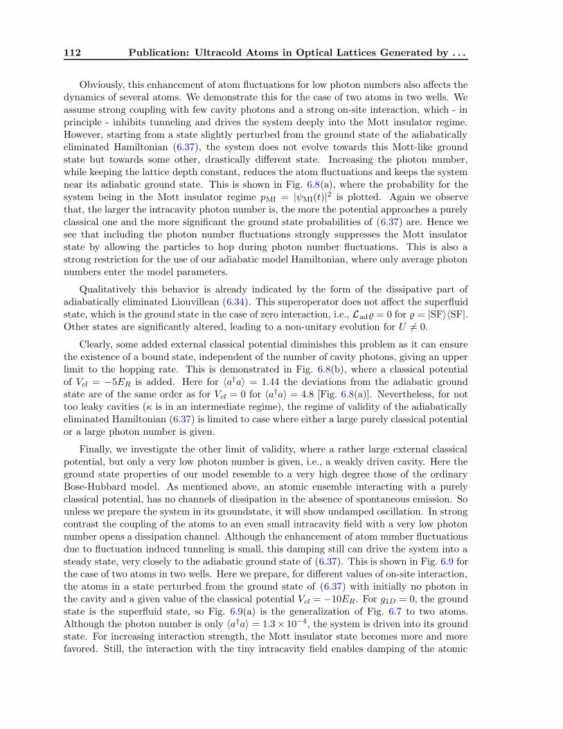
112 Publication: Ultracold Atoms in Optical Lattices Generated by . . .
Obviously, this enhancement of atom fluctuations for low photon numbers also affects thedynamics of several atoms. We demonstrate this for the case of two atoms in two wells. Weassume strong coupling with few cavity photons and a strong on-site interaction, which - inprinciple - inhibits tunneling and drives the system deeply into the Mott insulator regime.However, starting from a state slightly perturbed from the ground state of the adiabaticallyeliminated Hamiltonian (6.37), the system does not evolve towards this Mott-like groundstate but towards some other, drastically different state. Increasing the photon number,while keeping the lattice depth constant, reduces the atom fluctuations and keeps the systemnear its adiabatic ground state. This is shown in Fig. 6.8(a), where the probability for thesystem being in the Mott insulator regime pMI = |ψMI(t)|2 is plotted. Again we observethat, the larger the intracavity photon number is, the more the potential approaches a purelyclassical one and the more significant the ground state probabilities of (6.37) are. Hence wesee that including the photon number fluctuations strongly suppresses the Mott insulatorstate by allowing the particles to hop during photon number fluctuations. This is also astrong restriction for the use of our adiabatic model Hamiltonian, where only average photonnumbers enter the model parameters.
Qualitatively this behavior is already indicated by the form of the dissipative part ofadiabatically eliminated Liouvillean (6.34). This superoperator does not affect the superfluidstate, which is the ground state in the case of zero interaction, i.e., Lad% = 0 for % = |SF〉〈SF|.Other states are significantly altered, leading to a non-unitary evolution for U 6= 0.
Clearly, some added external classical potential diminishes this problem as it can ensurethe existence of a bound state, independent of the number of cavity photons, giving an upperlimit to the hopping rate. This is demonstrated in Fig. 6.8(b), where a classical potentialof Vcl = −5ER is added. Here for 〈a†a〉 = 1.44 the deviations from the adiabatic groundstate are of the same order as for Vcl = 0 for 〈a†a〉 = 4.8 [Fig. 6.8(a)]. Nevertheless, for nottoo leaky cavities (κ is in an intermediate regime), the regime of validity of the adiabaticallyeliminated Hamiltonian (6.37) is limited to case where either a large purely classical potentialor a large photon number is given.
Finally, we investigate the other limit of validity, where a rather large external classicalpotential, but only a very low photon number is given, i.e., a weakly driven cavity. Here theground state properties of our model resemble to a very high degree those of the ordinaryBose-Hubbard model. As mentioned above, an atomic ensemble interacting with a purelyclassical potential, has no channels of dissipation in the absence of spontaneous emission. Sounless we prepare the system in its groundstate, it will show undamped oscillation. In strongcontrast the coupling of the atoms to an even small intracavity field with a very low photonnumber opens a dissipation channel. Although the enhancement of atom number fluctuationsdue to fluctuation induced tunneling is small, this damping still can drive the system into asteady state, very closely to the adiabatic ground state of (6.37). This is shown in Fig. 6.9 forthe case of two atoms in two wells. Here we prepare, for different values of on-site interaction,the atoms in a state perturbed from the ground state of (6.37) with initially no photon inthe cavity and a given value of the classical potential Vcl = −10ER. For g1D = 0, the groundstate is the superfluid state, so Fig. 6.9(a) is the generalization of Fig. 6.7 to two atoms.Although the photon number is only 〈a†a〉 = 1.3× 10⁻⁴, the system is driven into its groundstate. For increasing interaction strength, the Mott insulator state becomes more and morefavored. Still, the interaction with the tiny intracavity field enables damping of the atomic

6.3. Cavity pump 113
Figure 6.8. (color online) Probability of the Mott insulator state |ψMI(t)|2 for twoatoms in two wells. Parameters and procedure as in Fig. 6.7, but due the second atomthe photon numbers are increased. The on-site interaction is U = 0.32ER. (a) Vcl = 0.The curves correspond to a mean photon number of 0.19 (solid line), 0.97 (dashed line),4.8 (dashed-dotted line) and 24.2 (dotted line). (b) Vcl = −5ER and correspondingphoton numbers of 0.05 (solid line), 0.28 (dashed line), 1.44 (dashed-dotted line).
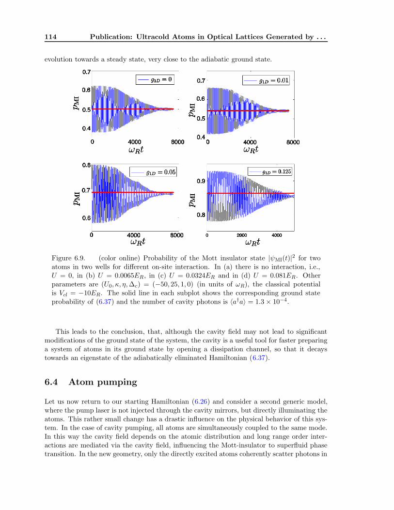
114 Publication: Ultracold Atoms in Optical Lattices Generated by . . .
evolution towards a steady state, very close to the adiabatic ground state.
Figure 6.9. (color online) Probability of the Mott insulator state |ψMI(t)|2 for twoatoms in two wells for different on-site interaction. In (a) there is no interaction, i.e.,U = 0, in (b) U = 0.0065ER, in (c) U = 0.0324ER and in (d) U = 0.081ER. Otherparameters are (U0, κ, η,∆c) = (−50, 25, 1, 0) (in units of ωR), the classical potentialis Vcl = −10ER. The solid line in each subplot shows the corresponding ground stateprobability of (6.37) and the number of cavity photons is 〈a†a〉 = 1.3× 10⁻⁴.
This leads to the conclusion, that, although the cavity field may not lead to significantmodifications of the ground state of the system, the cavity is a useful tool for faster preparinga system of atoms in its ground state by opening a dissipation channel, so that it decaystowards an eigenstate of the adiabatically eliminated Hamiltonian (6.37).
6.4 Atom pumping
Let us now return to our starting Hamiltonian (6.26) and consider a second generic model,where the pump laser is not injected through the cavity mirrors, but directly illuminating theatoms. This rather small change has a drastic influence on the physical behavior of this sys-tem. In the case of cavity pumping, all atoms are simultaneously coupled to the same mode.In this way the cavity field depends on the atomic distribution and long range order inter-actions are mediated via the cavity field, influencing the Mott-insulator to superfluid phasetransition. In the new geometry, only the directly excited atoms coherently scatter photons in

6.4. Atom pumping 115
the cavity mode. Due to the position-dependent coupling, the scattered field amplitude andphase for each atom is strongly position dependent. Atoms located at nodes are not coupledto the field, leading to no scattering, whereas atoms at antinodes are maximally coupled,leading to maximum scattering. Atoms in adjacent wells are separated by half a wavelengthand scatter with opposite phases, such that their contributions to the scattered field interferesdestructively. Naively one would thus immediately conclude that atoms forming a state witha homogeneous density scatter no field at all so that nothing happens [34, 35]. Nevertheless,fluctuations of the density still can allow for some background scattering which should dimin-ish for lower temperature. For suitable parameters the corresponding forces start to reorderthe atoms towards a periodic pattern of the atoms, where scattering is strongly enhanced.This then deepens the optical potential, stabilizing the pattern in a self-organizing runawayprocess, semiclassically described in [18].
At T = 0 quantum fluctuations still can trigger this reorganization. To study this effectwe assume the coherent pump field to form a broad plane wave propagating transversally tothe cavity axis (see Fig. 6.1) replacing cavity pumping. This means that we set η = 0 andthe Hamiltonian (6.26) for constant atom number N reads as follows:
H = (E + JVcl) B + ~ (U0J0N −∆c) a†a+
U
2C + ~U0Ja
†aB + ~ηeff
(
a+ a†)
J0D. (6.51)
Here we introduced the operator D =∑
k(−1)k+1nk describing the difference in atomnumber between odd and even sites. The corresponding Heisenberg equation for the cavityfield (6.27) reads as follows:
a =
i[
∆c − U0
(
J0N + JB)]
− κ
a− iηeffJ0D. (6.52)
Consequently the Heisenberg equation for the particle operators is:
bk =(
E + JVcl − iU0Ja†a)
(bk+1 + bk−1)− iηeffJ0
(
a+ a†)
(−1)k+1bk + Unkbk. (6.53)
Hence we see that the occupation number difference drives the cavity field, which thenin turn starts to dephase neighboring atom sites via the first term in the second line ofEq. (6.53). Note that this interesting part of the dynamics even survives for deeper latticeswhen J is negligibly small and J is of order unity. This will discussed in more detail usingvarious approximations below.
6.4.1 Field-eliminated Hamiltonian
Adiabatic elimination of the field variables is a bit more subtle here as compared to thecavity pump case discussed before. The scattering amplitude of light into the cavity modehere depends strongly on the atomic positions. Hence even small position changes have alarge influence on the cavity field dynamics. The maximum photon number is establishedwhen all the atoms are well localized at either only odd or only even lattice sites. For red

116 Publication: Ultracold Atoms in Optical Lattices Generated by . . .
atom field detuning this increases the lattice depth and forces the atoms into one of twostable patterns, where the wells where atoms are located are deeper than the empty ones.Hence this changes the translational periodicity of the optical lattice from λ/2 to λ. Suchbistable behavior was observed by Vuletic and coworkers [20] and explained in a semiclassicaltreatment [18].
Let us now turn to a quantum treatment of atoms and field. Naive adiabatic elimina-tion encounters a first difficulty, as the operators B, D do not commute, [B, D] 6= 0. Hencethis already creates an ordering problem in the formal steady-state solution of (6.52), whichgets even more difficult when it comes to the replacement of the field operators to obtainan effective Hamiltonian (6.51). Unfortunately also the second approach used in the caseof cavity pumping, namely reading off an effective Hamiltonian from the particle operatorHeisenberg equation does not resolve this problems. Replacing a with the steady-state ex-pression in (6.53) leads to a rather complex form, so that there is no simple way to find asuitable effective Hamiltonian Had, with i~bk = [bk,Had].
Hence we have to resort to the further approximation of neglecting the term ~U0Ja†aB,
compared to JVcl. This still leaves the most important part of the new physics, but reducesthe field equation to the form:
a =(
i∆′c − κ
)
a− iηeffJ0D. (6.54)
The steady-state solution of this equation is immediately at hand and free of orderingambiguities of non-commuting operators.
a =iηeffJ0
i∆′c − κ
D. (6.55)
Also the particle operator equation is much simpler within this approximation:
bk = (E + JVcl) (bk−1 + bk+1)− iηeffJ0
(
a+ a†)
(−1)k+1bk + Unkbk. (6.56)
In this form one then can find a well defined effective Hamiltonian only containing particleoperators. Let us thus proceed as in Sec. 6.3.1 and simply substitute (6.55) and its adjointinto (6.51). This yields the effective Hamiltonian:
Had = (E + JVcl)B +U
2+
~J20 η
2eff∆′
c
κ2 + ∆′c2 D
2. (6.57)
Within first order in J the replacement of the field variables in the Liouvillean part ofthe master equation (6.20) in this case does not provide an extra terms to be included in theHamiltonian. So the effective cavity decay induced dissipation on the atomic dynamics takesthe simple and intuitive form:
Lad% =κη2
effJ20
κ2 + ∆′c2
(
2D%D − D2%− %D2)
. (6.58)
Note that Eq. (6.57) with the replacement of the field operator by its steady-state ex-pression also leads to the same time evolution as induced by (6.56) after symmetrizing withrespect to the field terms. The two approaches thus lead to identical predictions, which wewill exhibit in some more detail in the following.

6.4. Atom pumping 117
6.4.2 Self-organization of atoms in an optical lattice
In this section we investigate the microscopic dynamics of self-ordering near zero temperatureand compare the results of the general model Hamiltonian (6.51) and the correspondingeffective Hamiltonian (6.57). In order to simplify things, we keep the approximation fromabove and neglect JU0a
†a in the model, i.e.,
H = (E + JVcl) B − ~∆′ca
†a+U
2C + ~ηeffJ0D
(
a+ a†)
, (6.59)
with ∆′c = ∆c − U0J0N . Let us point out here, that the Hamiltonian in this approximative
form is equivalent to a Hamiltonian describing 1D motion along an optical lattice transverseto the cavity axis. Such a lattice can e.g. be generated by the pump laser itself as it wasstudied in [55, 56] to investigate the onset of the self-organization process [18–20] at zerotemperature.
Similar to that case, the effective Hamiltonian Eq. (6.59) for moderate coupling repro-duces quite well the results of a full Monte-Carlo wavefunction simulation. We have checkedthis for a rather small system of two atoms in two wells with periodic boundary conditions.This is the minimal system to study self-organization but in general sufficient to capture thephysics. In this special case the operator B simply couples the ordered |11〉 state to thestate 1/
√2 (|20〉 + |02〉), while the operator D2 leaves all the basis states |11〉, |20〉, |02〉
unchanged. It simply leads to a relative energy shift. Hence starting from a perfectly or-dered atomic state (the analog of the Mott insulator state) the Hamiltonian part of the timeevolution of the system couples it to the symmetric superposition of ordered states. In anadiabatic limit those ordered states are correlated with a coherent field ±α in the cavity.Thus without damping the evolution would simply read:
|ψ(t)〉 = cos (2ωt) |11, 0〉 + i sin (2ωt)√2
(|20, 2α〉 + |02,−2α〉) . (6.60)
where the frequency ω is given by the (E + JVcl)/~. Here |11, 0〉 is the state with one atomin each well and zero photons, whereas |20, α〉 (|02,−α〉) corresponds to the state with bothatoms in the left (right) well, and the cavity field being in a coherent state with amplitude 2α(−2α). The factor 2 is due to constructive interference of the fields, scattered by the orderedatoms. In the Mott state, the scattering fields cancel each other.
Note that such an entangled superposition of different atomic states and fields cannotbe reproduced by any classical or mean field evolution and requires a genuine quantumdescription. If on-site interaction is added the amplitude of this oscillations decreases due toextra relative different phase changes of the self-ordered and the Mott state.
Of course we now have to add the effect of dissipation via cavity loss. We will see thateven single cavity photon decay events strongly perturb the system evolution. This can beimmediately seen by applying the photon annihilation operator to the entangled atom-fieldstate, i.e.,
|ψ(t)′〉 ∝ a|ψ(t)〉 ∝ |20, 2α〉 − |02,−2α〉. (6.61)

118 Publication: Ultracold Atoms in Optical Lattices Generated by . . .
This procedure projects out the Mott contributions to the state as they are connected tozero photons. Surprisingly in addition it also blocks further tunneling by introducing a minussign between the two ordered states. At this point coherent atomic time evolution stops until asecond photon escapes and re-establishes the plus sign. This then allows tunnel coupling backto the Mott insulator state again. In this sense self-ordering is an instantaneous projectiveprocess here, where the cavity acts as measurement apparatus asking a sort of yes/no orderingquestion.
The fact, that for transverse pumping the adiabatic field state associated to the Mottinsulator is an intracavity vacuum decouples this state from further dynamics even in thepresence of dissipation. This creates numerical difficulties and prohibits an approximation ofthe dissipative dynamics by the adiabatic ground state values of (6.57) only. As soon as aphoton leaks out of the cavity, the contribution of the Mott-insulator state is canceled, nomatter how large it, corresponding to a given on-site interaction, might be. Hence, everyinitial state evolves into a superposition of the ordered states and the ground state values ofthe effective Hamiltonian do not make much sense. Nevertheless, including the damping viathe effective Liouvillean (6.58) approximately reveals the complete dynamics. In Fig. 6.10 weshow the results of a Monte-Carlo simulation of the dynamics of the Mott and the superfluidcontribution, corresponding to (6.59) and compare it with a solution of the master equation,consisting of the Hamiltonian (6.57) and Liouvillean (6.58), where the field variables areeliminated. Furthermore, the restriction of the Hilbert space to the two states of (6.61) and|11, 0〉, allows for a proof of the accuracy of our assumption, concerning the fast evolution ofthe cavity field. We use the coefficients c(t), c(t) (calculated with the Monte Carlo simulation)of |ψ(t)〉 = c(t)|11, 0〉 + c(t)(|20, 2α〉 ± |02,−2α〉) to construct a purely atomic state |ϕ(t)〉 =c(t)|11〉 + c(t)(|20〉 ± |02〉). Then the mean photon number, calculated with the effectivephoton operator (6.55) agrees very well with the real mean photon number, i.e.,
η2effJ
20
∆′c2 + κ2
〈ϕ(t)|D2|ϕ(t)〉 ≈ 〈ψ(t)|a†a|ψ(t)〉. (6.62)
6.5 Conclusions
Based on an approximative Bose-Hubbard type model descriptions, we have shown thatquantum characteristics of light fields generating optical potentials lead to shifts in quantumphase transition points and play a decisive role in the microscopic dynamics of the transitionprocess. While many physical aspects can be already captured by effective Hamiltonianswith rescaled parameters, cavity mediated long-range interactions also play an importantrole and add a new nonlocal element to optical lattices dynamics for atoms. In that contexteven small modifications in the setup, from cavity pump to transverse pump, have a drasticinfluence on the behavior of the system on a microscopic level. We have seen that theBose-Hubbard Hamiltonian for the former system can, in a certain parameter regime, besignificantly simplified by adiabatically eliminating the field variables. Although the cavityhas influence on its shape, the Mott insulator to superfluid phase transition occurs similarto classical optical lattices. For transverse pumping this is not the case. Here, the fieldsscattered by the atoms in the uniform Mott state cancel and completely suppress scattering.In parallel new ordered states with maximal coupling of pump and cavity field appear and
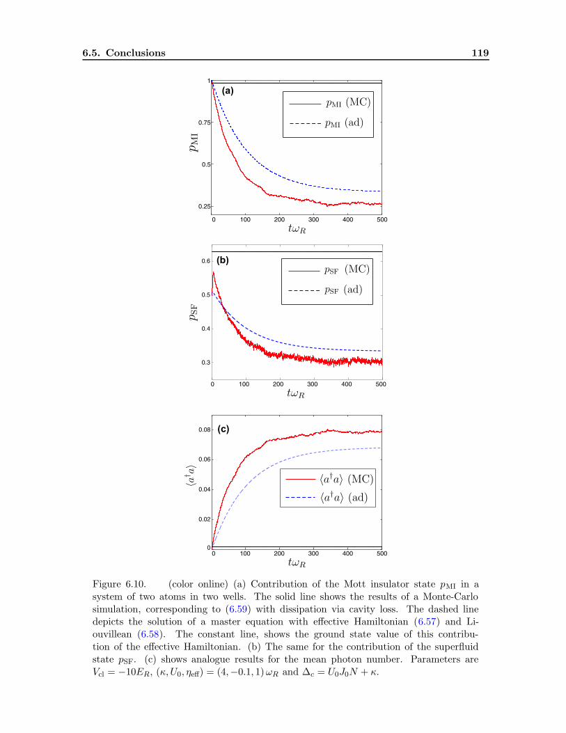
6.5. Conclusions 119
(c)
Figure 6.10. (color online) (a) Contribution of the Mott insulator state pMI in asystem of two atoms in two wells. The solid line shows the results of a Monte-Carlosimulation, corresponding to (6.59) with dissipation via cavity loss. The dashed linedepicts the solution of a master equation with effective Hamiltonian (6.57) and Li-ouvillean (6.58). The constant line, shows the ground state value of this contribu-tion of the effective Hamiltonian. (b) The same for the contribution of the superfluidstate pSF. (c) shows analogue results for the mean photon number. Parameters areVcl = −10ER, (κ,U0, ηeff) = (4,−0.1, 1)ωR and ∆c = U0J0N + κ.
120 Publication: Ultracold Atoms in Optical Lattices Generated by . . .
the dynamics favors a superposition of these two ordered states correlated with coherent fieldstates with phase difference π. Hence the dynamics generates strong atom field entanglementand large effective optical nonlinearities even in the limit of linear weak field scattering.
Of course the various approximations used to derive our effective Hamiltonians still leavea lot of room for improvements and we could only touch a very small part of the physicaleffects and possibilities contained in these model. Fortunately the experimental progress inthis field is spectacularly fast and several groups now have set up optical lattices with cavityfields [36–39] and intriguing potential applications of such systems were already proposed [57],so that one can expect a fast and exciting further development of this field.
Acknowledgments
The authors would like to thank M. Lewenstein, G. Morigi, S. Fernandez-Vidal, A. Micheli,and A. Vukics for useful discussions. This work was funded by the Austrian Science Fund(P17709 and S1512). After completion of this work we became aware of related parallel workby M. Lewenstein and coworkers, which treats many aspects of this model in the thermody-namic limit [58].
Bibliography
[1] See e.g. Laser Manipulation of Atoms and Ions, ed. by E. Arimondo and W. D. Phillips,Varenna Summer School, 1991 (North-Holland, Amsterdam 1992).
[2] I. Bloch, Nature Physics 1, 23 (2005); I. Bloch and M. Greiner, Adv. At. Mol. Opt.Phys. 52, 1 (2005).
[3] D. Jaksch, C. Bruder, J. I. Cirac, C. W. Gardiner, and P. Zoller, Phys. Rev. Lett. 81,3108 (1998);
[4] W. Zwerger, J. Opt. B 5, 9 (2003).
[5] M. P. A. Fisher, P. B. Weichman, G. Grinstein, and D. S. Fisher, Phys. Rev. B 40, 546(1989).
[6] M. Greiner, O. Mandel, T. Esslinger, T. W. Hansch, and I. Bloch, Nature (London) 415,39 (2002); M. Greiner, O. Mandel, T. W. Hansch and I. Bloch, Nature (London) 419,51 (2002).
[7] D. Jaksch and P. Zoller, Ann. Phys. 315, 52 (2005).
[8] S. Inouye, M. R. Andrews, J. Stenger, H. -J. Miesner, D. M. Stamper-Kurn and W.Ketterle, Nature (London) 392, 151 (1998).
[9] M. Theis, G. Thalhammer, K. Winkler, M. Hellwig, G. Ruff, R. Grimm, and J. HeckerDenschlag, Phys. Rev. Lett. 93, 123001 (2004).

BIBLIOGRAPHY 121
[10] T. Stoferle, H. Moritz, C. Schori, M. Kohl, and T. Esslinger, Phys. Rev. Lett. 92, 130403(2004).
[11] M. Kohl, H. Moritz, T. Stoferle, C. Schori and T. Esslinger, J. Low Temp. Phys. 138,635 (2005).
[12] I. B. Spielman, W. D. Phillips, and J. V. Porto, Phys. Rev. Lett. 98, 080404 (2007).
[13] B. Paredes, A. Widera, V. Murg, O. Mandel, S. Folling, I. Cirac, G. V. Shlyapnikov, T.W. Hansch and I. Bloch, Nature (London) 429, 277 (2004).
[14] T. Kinoshita, T. R. Wenger, and D. S. Weiss, Science 305, 1125 (2004).
[15] Z. Hadzibabic, P. Kruger, M.Cheneau, B. Battelier, and J. Dalibard, Nature (London)441, 1118 (2006).
[16] M. Lewenstein, A. Sanpera, V. Ahufinger, B. Damski, A. Sen De, and U. Sen, Adv.Phys. 56, 243 (2007).
[17] P. Domokos and H. Ritsch, J. Opt. Soc. Am. B 20, 1098 (2003).
[18] P. Domokos and H. Ritsch, Phys. Rev. Lett. 89, 253003 (2002).
[19] S. Zippilli, G. Morigi, and H. Ritsch, Phys. Rev. Lett. 93, 123002 (2004).
[20] A. T. Black, H. W. Chan, and V. Vuletic, Phys. Rev. Lett. 91, 203001 (2003).
[21] P. W. H. Pinkse, T. Fischer, P. Maunz, and G. Rempe, Nature (London) 404, 365(2000).
[22] C. J. Hood, T. W. Lynn, A. C. Doherty, A. S. Parkins, and H. J. Kimble, Science 287,1447 (2000).
[23] P. Horak, G. Hechenblaikner, K. M. Gheri, H. Stecher, and H. Ritsch, Phys. Rev. Lett.79, 4974 (1997); G. Hechenblaikner, M. Gangl, P. Horak, and H. Ritsch, Phys. Rev. A58, 3030 (1998).
[24] V. Vuletic, H. W. Chan, and A. T. Black, Phys. Rev. A 64, 033405.
[25] P. Domokos, A. Vukics, and H. Ritsch, Phys. Rev. Lett. 92, 103601 (2004).
[26] S. Zippilli, G. Morigi, and H. Ritsch, Phys. Rev. Lett. 95, 143001 (2005).
[27] P. Maunz, T. Puppe, I. Schuster, N. Syassen, P. W. H. Pinkse, and G. Rempe, Nature(London) 428, 50 (2004).
[28] S. Nußmann, K. Murr, M. Hijlkema, B. Weber, A. Kuhn, and G. Rempe, Nature Physics1, 122 (2005).
[29] A. Griessner, D. Jaksch, and P. Zoller, J. Phys. B 37, 1419 (2004).
[30] P. Horak, S. M. Barnett, and H. Ritsch, Phys. Rev. A 61, 033609 (2000).

122 Publication: Ultracold Atoms in Optical Lattices Generated by . . .
[31] D. Jaksch, S. A. Gardiner, K. Schulze, J. I. Cirac, and P. Zoller, Phys. Rev. Lett. 86,4733 (2001).
[32] C. Maschler and H. Ritsch, Phys. Rev. Lett. 95, 260401 (2005).
[33] J. Larsson, B. Damski, G. Morigi, and M. Lewenstein, arXiv:cond-mat/0608335.
[34] I. B. Mekhov, C. Maschler, and H. Ritsch, Phys. Rev. Lett. 98, 100402 (2007); I. B.Mekhov, C. Maschler, and H. Ritsch, Phys. Rev. A (accepted).
[35] I. B. Mekhov, C. Maschler, and H. Ritsch, Nature Physics 3, 319 (2007).
[36] A. Ottl, S. Ritter, M. Kohl, and T. Esslinger, Phys. Rev. Lett. 95 090404 (2005); T.Bourdel, T. Donner, S. Ritter, A. Ottl, M. Kohl, and T. Esslinger, Phys. Rev. A 7343602 (2006).
[37] P. Treutlein, D. Hunger, S. Camerer, T. W. Hansch, and J. Reichel, Phys. Rev. Lett.99, 140403 (2007); Y. Colombe, T. Steinmetz, G. Dubois, F. Linke, D. Hunger, and J.Reichel, arXiv:quant-ph/0706.1390.
[38] S. Slama, G. Krenz, S. Bux, C. Zimmermann, and Ph. W. Courteille, Phys. Rev. A 75,063620 (2007).
[39] S. Gupta, K. L. Moore, K. W. Murch, and D. M. Stamper-Kurn, arXiv:quant-ph/0706.1052.
[40] J. McKeever, J. R. Buck, A. D. Boozer, A. Kuzmich, H. -C. Nagerl, D. M. Stamper-Kurn,and H. J. Kimble, Phys. Rev. Lett. 90, 133602 (2003).
[41] T. Puppe, I. Schuster, P. Maunz, K. Murr, P. W. H. Pinkse, and G. Rempe, Phys. Rev.Lett. 99, 013002 (2007).
[42] E. T. Jaynes and F. W. Cummings, Proc. IEEE 51, 89 (1963).
[43] See, for example, A. Galindo and P. Pascual, Quantum Mechanics II, (Springer, Berlin,1990).
[44] K. Huang, Statistical Mechanics, (John Wiley & Sons, New York, 1987).
[45] It is also possible, to eliminate the excited state first in the single particle dynamics,which leads to the same expression (6.18) and then implement this expression in secondquantization formalism.
[46] M. Olshanii, Phys. Rev. Lett. 81, 938 (1998).
[47] C. Maschler and H. Ritsch, Phys. Rev. Lett. 95, 260401 (2005).
[48] C. Kittel, Quantum Theory of Solids, (John Wiley & Sons, New York, 1963).
[49] See, for example, C. W. Gardiner and P. Zoller, Quantum Noise, 3rd Ed. (Springer,Berlin, 2005).

BIBLIOGRAPHY 123
[50] R. Grimm, M. Weidemuller, and Y. B. Ovchinnikov, Adv. At. Mol. Opt. Phys. 42, 95(2000).
[51] J. Ye, D. W. Vernooy, and H. J. Kimble, Phys. Rev. Lett. 83, 4987 (1999).
[52] J. A. Sauer, K. M. Fortier, M. S. Chang, C. D. Hamley, and M. S. Chapman, Phys. Rev.A 69, 051804 (2004).
[53] H. M. Wiseman and G. J. Milburn, Phys. Rev. A 47, 642 (1993).
[54] A. Vukics and H. Ritsch, Eur. J. Phys. D 44, 585 (2007).
[55] C. Maschler, H. Ritsch, A. Vukics, and P. Domokos, Opt. Comm. 273, 446 (2007).
[56] A. Vukics, C. Maschler, and H. Ritsch, New J. Phys. 9, 255 (2007).
[57] D. Meiser, J. Ye, and M. J. Holland, arXiv:quant-ph/0707.3834.
[58] J. Larson, S. Fernandez-Vidal, G. Morigi, and M. Lewenstein, arXiv:cond-mat/0710.3047.


Part II
Probing Atomic Phases in OpticalLattices


Chapter 7
Publication
Cavity Enhanced Light Scattering in Optical Lattices toProbe Atomic Quantum Statistics†
Physical Review Letters 98, 100402 (2007)
I. B. Mekhov1,2, C. Maschler1, and H. Ritsch1
1) Institut fur theoretische Physik, Universitat Innsbruck,A-6020 Innsbruck, Austria
2) St. Petersburg State University, V. A. Fock Institute of Physics,St. Petersburg, Russia
Different quantum states of atoms in optical lattices can be nondestructively moni-tored by off-resonant collective light scattering into a cavity. Angle resolved measurementsof photon number and variance give information about atom-number fluctuations and paircorrelations without single-site access. Observation at angles of diffraction minima pro-vides information on quantum fluctuations insensitive to classical noise. For transverseprobing, no photon is scattered into a cavity from a Mott insulator phase, while thephoton number is proportional to the atom number for a superfluid.
Studies of ultracold atoms in optical lattices link various disciplines. Fundamental quan-tum many-body theories, formulated initially for condensed matter, can be tested in bettercontrollable atomic systems [1], e.g., strongly correlated phases, quantum simulators. Suchstudies influence different areas [1]: quantum information processing, ultracold collisions,exotic molecules, etc.
While mean-field approaches describe only the average atomic density, the main goal isto study quantum properties of these gases. They are most prominent in lattices, whereone has phase transitions between states of similar density but radically different quantumfluctuations.
Standard methods to measure quantum properties are based on matter-wave interfer-ence of atoms released from a trap [2] destroying the system. “Bragg spectroscopy” usingstimulated matter-wave scattering by laser pulses proved successful [3, 4] but destructive.
†The primary contribution of the author of the present thesis performed to this publication was the instal-lation of the model and the calculation of certain generic examples and statistical quantities (cf. Table 7.1).He also acted as a discussion partner on all other aspects of the work.

128 Publication: Cavity Enhanced Light Scattering to Probe . . .
probe a0
scattered light a1
d
0
1
probe a0
scattered light a1
d
0
1
Figure 7.1. Setup: A lattice is illuminated by a probe at the angle θ0 which is scatteredinto a cavity at θ1.
Alternative less destructive methods observing scattered light were proposed mainly for ho-mogeneous Bose-Einstein condensates (BEC) [5–8], but not yet implemented.
Here we show that specifically for periodic lattices, light scattering can help to overcomeexperimental difficulties. In contrast to homogeneous BECs, scattering from a lattice allowsto determine local and nonlocal correlations without single-atom optical access using thesuppression of strong classical scattering at Bragg minima and monitoring much richer angulardistributions. This looks extremely useful for studying phase transitions between, e.g., Mottinsulator (MI) and superfluid (SF) states, without destruction, since various quantum phasesshow even qualitatively distinct scattering.
Joining two fields, cavity quantum electrodynamics (QED) and ultracold gases, will enablenew investigations of both light and matter at ultimate quantum levels, which only recentlybecame experimentally possible [9].
Our model is based on nonresonant interaction, not relying on a particle level structure.Thus it also applies to molecular physics, where new quantum phases were obtained [10].It can be also applied for semiconductors [11], as, e.g., were used for BEC of exciton-polaritons [12].
Model. We consider N two-level atoms in an optical lattice with M sites. A region ofK ≤M sites is illuminated by probe light which is scattered into another mode (cf. Fig. 7.1).Although, each mode could be a freely propagating field, we will consider cavity modeswhose geometries (i.e. axis directions or wavelengths) can be varied. A related manybody
129
Hamiltonian is given by
H =∑
l=0,1
~ωla†l al +
∫
d3rΨ†(r)Ha1Ψ(r), (7.1a)
Ha1 =p2
2ma+ Vcl(r) + ~g2
0
∑
l,m=0,1
u∗l (r)um(r)a†l am∆ma
, (7.1b)
where a0 (a1) are the annihilation operators of the probe (scattered) light with the frequenciesω0,1, wave vectors k0,1, and mode functions u0,1(r); Ψ(r) is the atom-field operator. In theeffective single-atom Hamiltonian Ha1, p and r are the momentum and position operatorsof an atom of mass ma trapped in a classical potential Vcl(r); g0 is the atom–light couplingconstant. We consider the field-atom detunings ∆la = ωl − ωa larger than the spontaneousemission rate and Rabi frequencies. Thus, in Ha1 the adiabatic elimination of the upper statewas used.
Assuming weak fields a0,1, we expand Ψ(r) in Eq. (7.1a) using localized Wannier func-tions corresponding to Vcl(r) and keep only the lowest vibrational state at each site:Ψ(r) =
∑Mi=1 biw(r− ri), where bi is the atom annihilation operator at site with coordi-
nate ri. Substituting this in Eq. (7.1a), one can get a generalized Bose-Hubbard Hamiltonian[1] including light scattering. However, in contrast to our previous work [13] and “Braggspectroscopy” [4], we do not consider lattice excitations here and focus on scattering fromatoms in a prescribed state.
Neglecting atomic tunneling, the Hamiltonian reads:
H =∑
l=0,1
~ωla†lal + ~g2
0
∑
l,m=0,1
a†lam∆ma
(
K∑
i=1
J lmi,i ni
)
, (7.2)
where ni = b†i bi. We define the operator of the atom number at illuminated sites as
NK =∑K
i=1 ni. For a deep lattice the coefficients J lmi,i =∫
drw2(r − ri)u∗l (r)um(r) reduce
to J lmi,i = u∗l (ri)um(ri) neglecting atom spreading, which can be studied even by classicalscattering [14].
The Heisenberg equation for the scattered light in the frame rotating with ω0 (∆01 =ω0 − ω1) thus reads:
a1 = i
[
∆01 −g20
∆1a
K∑
i=1
|u1(ri)|2ni]
a1 − ig20a0
∆0a
K∑
i=1
u∗1(ri)u0(ri)ni − κa1, (7.3)
where κ is the cavity decay rate and a0 will be assumed a classical field given by a c-numberconstant.
Light properties. Though the dispersion shift of a cavity mode is sensitive to atomstatistics through ni, we assume it is much smaller than κ or ∆01. A stationary solution ofEq. (7.3) for a1 and photon number then reads

130 Publication: Cavity Enhanced Light Scattering to Probe . . .
a1 = CD, nph = a†1a1 = |C|2D∗D, D =
K∑
i=1
Aini, (7.4)
with C ≡ ig20a0/[∆0a(i∆01−κ)] and the coefficients Ai(θ0, θ1) ≡ u∗1(ri)u0(ri). This expression
of the light operators through the atomic ones is a central result here.
For a 1D lattice of period d and atoms trapped at xm = md (m = 1, 2, ...,M) the modefunctions are u0,1(rm) = exp(imk0,1xd) for traveling and u0,1(rm) = cos(mk0,1xd) for standingwaves with k0,1x = |k0,1| sin θ0,1 (cf. Fig. 7.1). For the atomic quantum state we use theassumptions: (i) the mean atom number at all sites is 〈ni〉 = n = N/M (〈NK〉 = NK ≡ nK)and (ii) the pair correlations 〈ninj〉 are identical for any i 6= j, which is valid for a deeplattice, and will be denoted as 〈nanb〉 (with a 6= b).
Thus, 〈a1〉 ∼ 〈D〉 =∑K
i=1Ai〈ni〉 = nA showing that the field amplitude only dependson the mean density and exhibits the angular distribution of classical diffraction A(θ0, θ1) ≡∑K
i=1Ai(θ0, θ1) with diffraction maxima and minima. The central point now is that thephoton number (7.4) is not just the amplitude squared, but we get
〈D∗D〉 =〈nanb〉|A|2 + (〈n2〉 − 〈nanb〉)K∑
i=1
|Ai|2, (7.5a)
R(θ0, θ1) ≡〈D∗D〉 − |〈D〉|2 = 〈δnaδnb〉|A|2 + (〈δn2〉 − 〈δnaδnb〉)K∑
i=1
|Ai|2, (7.5b)
where δni ≡ ni− n giving 〈δnaδnb〉 = 〈nanb〉 − n2, and 〈δn2〉 equal to the variance (∆ni)2 =
〈n2i 〉−n2. Thus, the intensity is sensitive to atomic quantum statistics via the density-density
correlations 〈ninj〉 different for particular states. Besides the classical angle dependence |A|2,the second term in Eq. (7.5a) reflects fluctuations and has a completely different dependence.Particularly in a lattice, scattering is sensitive not only to the periodic density, but also toperiodic fluctuations, leading to the observable difference between states with and withoutnonlocal correlations. Analysis of quadrature variances gives results similar to analysis of thenoise quantity R.
For two traveling waves, Eq. (7.5a) gives the structure factor considered in Ref. [7] onhomogeneous BECs. We show that a more general form including standing waves gives newmeasurable quantities beyond structure factor.
The intensity fluctuations of the scattered light depend on the fourth moments of theatomic number operators and four-point density correlations 〈ninjnknl〉. For example thephoton-number variance is given by
(∆nph)2 = 〈n2ph〉 − 〈nph〉2 = |C|4(〈|D|4〉 − 〈|D|2〉2) + |C|2〈|D|2〉. (7.6)
To discuss examples of different scattering we summarize statistical properties of typicalstates in Table 7.1. For light scattering, the most classical state corresponding to pointlike

131
atoms is MI. Here the atom number at each site ni does not fluctuate and we have no paircorrelations. Hence we see from Eq. (7.5a) that the zeros of classical diffraction [A(θ0, θ1) = 0]are zeros of light intensity.
MI SF Coherent
|Ψ〉M∏
i=1
|ni〉i1√
MNN !(
M∑
i=1
b†i )N |0〉 e−
N2
M∏
i=1
e
q
NMb†i |0〉i
〈n2i 〉 n2 n2(1− 1/N) + n n2 + n
(∆ni)2 0 n(1− 1/M) n
〈N2K〉 N2
K N2K(1− 1/N) +NK N2
K +NK
(∆NK)2 0 NK(1−K/M) NK
〈nanb〉 n2 n2(1− 1/N) n2
〈δnaδnb〉 0 −N/M 2 0
Table 7.1. Various statistical quantities of typical quantum atomic states, namely theMott insulator state, the coherent state and the superfluid state.
This is different for a SF where each atom is delocalized over all sites leading to numberfluctuations at a given site and at K < M sites; the atoms at different sites are anticorrelated.At a classical diffraction zero we still find a photon number proportional to the atom numberN .
A coherent state approximates a SF but without pair correlations. In the limitN,M →∞,it well describes scattering from a small region (K M) of a partially illuminated superfluid(SFK). However, we proved that even in this limit it fails to describe scattering at angles ofBragg maxima from a large lattice region (K ∼M).
Example. Let us now show the most striking predictions of this model at the basicexample of a probe transverse to the lattice (θ0 = 0, cf. Fig. 7.1). The scattered lightis collected in a cavity along the lattice (θ1 = π/2) with atoms trapped at the antinodes(d = λ/2) [13, 15].
The operator D =∑K
k=1(−1)k+1nk (7.4) here gives almost zero average field amplitudeindependently on the atomic state. This reflects the opposite phase of light scattered fromatoms separated by λ/2 (diffraction minimum). However, the cavity photon-number is pro-portional to 〈D∗D〉 = (〈n2〉 − 〈nanb〉)K [cf. Eq. (7.5a)], which is determined by statistics ofa particular state. Thus, atoms in a MI state scatter no photons, while a SF scatters numberof photons proportional to the atom number:
〈a1〉MI = 〈a1〉SF = 0, but
〈a†1a1〉MI = 0, 〈a†1a1〉SF = |C|2NK .
Moreover, the photon number fluctuations (∆nph)2 are also different for various atomic
states. In the MI state, the variance (∆|D|2)2MI = 〈|D|4〉MI − 〈|D|2〉2MI = 0, whereas in SF,there is a strong noise (∆|D|2)2SF ≈ 2N2
K .

132 Publication: Cavity Enhanced Light Scattering to Probe . . .
Coupled light-matter dynamics in a cavity can lead to a new self-organized phase [15]with atoms trapped at every second site (d = λ), which gives D =
∑Kk=1 nk = NK (7.4). If
this state is a MI with d = λ, the number of photons 〈a†1a1〉Self-org = |C|2N2K is proportional
to the atom number squared and has a superradiant character.
Figure 7.2. Intensity angular distributions for two traveling waves. (a) Intensity ofclassical diffraction; (b) noise quantity R (7.7) for coherent atomic state (constant 1, lineA), SF with all sites illuminated K = M (curve B), and MI state (constant 0, line C);(c) the same as in (b) but for partially illuminated SF with K = M/2. N = M = 30,θ0 = 0.
Angular distributions. We will quantitatively discuss angular intensity distributionsfor scattering between two traveling waves, where Eq. (7.5b) reduces to
R = 〈δnaδnb〉sin2 (Kα−/2)
sin2 (α−/2)+ (〈δn2〉 − 〈δnaδnb〉)K. (7.7)
While |A|2 in the first term reproduces classical diffraction with α− = k0xd sin θ0 −k1xd sin θ1, the second term in Eq. (7.5b) is simply isotropic. Thus, the noise quantity iszero for MI, RMI = 0, nonzero but isotropic for the coherent state, RCoh = NK , and angledependent for a SF. In a SF, even small pair correlations 〈δnaδnb〉 = −N/M 2 give a largecontribution near diffraction maxima (α− = 2πl, l = 0, 1, ..), where the geometric factor isK2, invalidating the coherent-state approximation.
Figure 7.2 displays those angular distributions. Classical diffraction |〈D〉|2 with the onlypossible zero-order maxima at θ1 = 0, π (d = λ0,1/2, θ0 = 0) is shown in Fig.7.2(a). R for
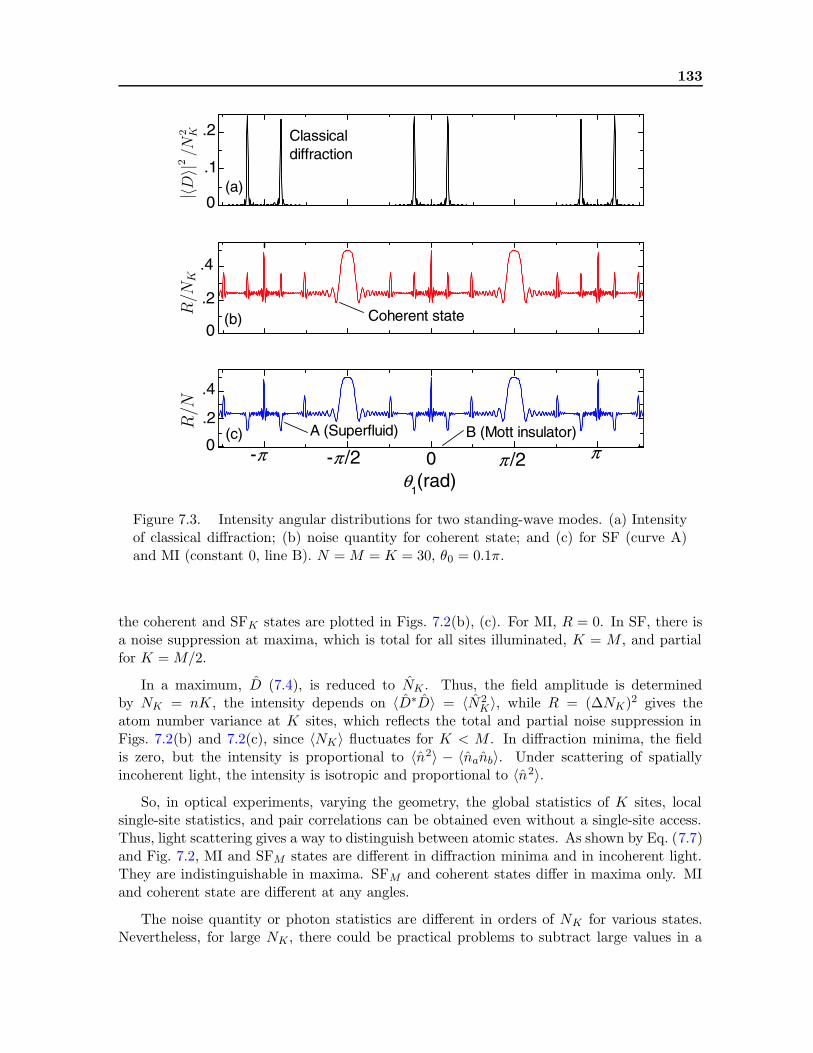
133
Figure 7.3. Intensity angular distributions for two standing-wave modes. (a) Intensityof classical diffraction; (b) noise quantity for coherent state; and (c) for SF (curve A)and MI (constant 0, line B). N = M = K = 30, θ0 = 0.1π.
the coherent and SFK states are plotted in Figs. 7.2(b), (c). For MI, R = 0. In SF, there isa noise suppression at maxima, which is total for all sites illuminated, K = M , and partialfor K = M/2.
In a maximum, D (7.4), is reduced to NK . Thus, the field amplitude is determinedby NK = nK, the intensity depends on 〈D∗D〉 = 〈N2
K〉, while R = (∆NK)2 gives theatom number variance at K sites, which reflects the total and partial noise suppression inFigs. 7.2(b) and 7.2(c), since 〈NK〉 fluctuates for K < M . In diffraction minima, the fieldis zero, but the intensity is proportional to 〈n2〉 − 〈nanb〉. Under scattering of spatiallyincoherent light, the intensity is isotropic and proportional to 〈n2〉.
So, in optical experiments, varying the geometry, the global statistics of K sites, localsingle-site statistics, and pair correlations can be obtained even without a single-site access.Thus, light scattering gives a way to distinguish between atomic states. As shown by Eq. (7.7)and Fig. 7.2, MI and SFM states are different in diffraction minima and in incoherent light.They are indistinguishable in maxima. SFM and coherent states differ in maxima only. MIand coherent state are different at any angles.
The noise quantity or photon statistics are different in orders of NK for various states.Nevertheless, for large NK , there could be practical problems to subtract large values in a

134 Publication: Cavity Enhanced Light Scattering to Probe . . .
maximum. In Refs. [6], this even led to a conclusion about the state indistinguishability byintensity measurements. In contrast to homogeneous BECs, in lattices, this problem has anatural solution: measurements outside maxima are free of the strong classical-like part ofscattering and thus directly reflect fluctuations.
A classical analogy of different light scattering consists in different density fluctuations. Aquantum treatment gives a deeper insight. Superfluid state is a superposition of all possiblemultisite Fock states giving distributions of N atoms at M sites. Various Fock states becomeentangled to scattered light of different phases and amplitudes. In contrast to a classical case(and MI with the only multisite Fock state), light fields entangled to various distributionsdo not interfere with each other due to the orthogonality of the Fock states. This reflectsthe which way information and explains the zero amplitude but nonzero photon number in adiffraction minimum.
If at least one of the modes is a standing wave, the angle dependences become much richer.Besides new classical maxima given by α± = k0xd sin θ0±k1xd sin θ1, the second, “noise,” termin Eqs. (7.5a) and (7.5b) is also not isotropic. It includes a sum of the geometric coefficientssquared, which is equivalent to effective doubling of the lattice period (or light frequencydoubling) leading to new features at angles, where classical diffraction predicts zero. InFig. 7.3, a case of two standing waves is shown. Due to the effective period doubling (givenby 2α0,1 = 2k0,1xd sin θ0,1 and 2α±), new features at the angles of, e.g., effective first-ordermaxima appear, though classically only the zero-order maxima are still possible.
The angle dependence of the photon number variance (∆nph)2 determined by (∆|D|2)2shows anisotropic features due to “period doubling” even for two traveling waves. For thecoherent state, the light at a maximum displays strong noise [(∆|D|2)2 = 4N3
K + 6N2K +Nk
because 〈|D|4〉 = N4K+6N3
K +7N2K +Nk and 〈|D|2〉 = N2
K+NK ], stronger than the isotropiccomponent (N 2
K in highest order of NK) and new features at θ1 = ±π/2 (for θ0 = 0, 2N2K in
highest order of NK). In SFM , the noise at maxima can be suppressed, while at other anglesit is nearly equal to that of the coherent state. In MI, (∆|D|2)2 = 0. Distinguishing betweenatomic states by light statistics is similar to that by the intensity.
In summary, we have shown that atomic quantum states can be nondestructively moni-tored by measuring scattered light. In contrast to homogeneous BECs, scattering from latticesexhibits advantageous properties: suppression of the classical scattering in Bragg minima, ac-cess to local and nonlocal correlations, angular distributions richer than classical diffraction.Also other optical phenomena and quantities depending nonlinearly on the atom numberoperators will reflect quantum atom statistics [16, 17], e.g., the dispersion of a medium willprovide a spectral method of quantum state characterization. Exploiting quantum propertiesof light should be applicable to other Bragg spectroscopy setups.
Support by: Austrian Science Fund (P17709, S1512).
Bibliography
[1] D. Jaksch et al., Phys. Rev. Lett. 81, 3108 (1998); I. Bloch, Nat. Phys. 1, 23 (2005).
[2] S. Folling et al., Nature 434, 481 (2005); E. Altman, E. Demler, and M. Lukin, Phys.Rev. A 70, 013603 (2004).

BIBLIOGRAPHY 135
[3] J. Stenger et al., Phys. Rev. Lett. 82, 4569 (1999).
[4] T. Stoferle et al., Phys. Rev. Lett. 92, 130403 (2004).
[5] L. You, M. Lewenstein, and J. Cooper, Phys. Rev. A 51, 4712 (1995).
[6] J. I. Cirac, M. Lewenstein, and P. Zoller, Phys. Rev. Lett. 72, 2977 (1994); Z. Idziaszek,K. Rzazewski, and M. Lewenstein, Phys. Rev. A 61, 053608 (2000).
[7] J. Javanainen and J. Ruostekoski, Phys. Rev. A 52, 3033 (1995); Phys. Rev. Lett. 91,150404 (2003).
[8] M. G. Moore, O. Zobay, and P. Meystre, Phys. Rev. A 60, 1491 (1999).
[9] A. Ottl et al., Phys. Rev. Lett. 95, 090404 (2005); I. Teper, Y. Lin, and V. Vuletic, ibid.97, 023002 (2006).
[10] T. Volz et al., Nat. Phys. 2, 692 (2006); K. Winkler et al., Nature 441, 853 (2006).
[11] M. Kira and S. W. Koch, Phys. Rev. A 73, 013813 (2006).
[12] J. Kasprzak et al., Nature 443, 409 (2006).
[13] C. Maschler and H. Ritsch, Phys. Rev. Lett. 95, 260401 (2005).
[14] S. Slama et al., Phys. Rev. Lett. 94, 193901 (2005); Phys. Rev. A 73, 023424 (2006).
[15] P. Domokos and H. Ritsch, Phys. Rev. Lett. 89, 253003 (2002); A. Black, J. Thompson,and V. Vuletic, J. Phys. B 38, S605 (2005).
[16] After having finished this work, we became aware of a related research of P. Meystre.We are grateful for sending us the preprint quant-ph/0610029 and discussions.
[17] I. Mekhov, C. Maschler, and H. Ritsch, in Books of abstracts for XX Int. Conference onAtomic Physics, ICAP, Innsbruck, 2006, p. 309 and conference web-site.


Chapter 8
Publication
Light Scattering from Ultracold Atoms in Optical Lattices as
an Optical Probe of Quantum Statistics†
quant-ph/0702193 (accepted for publication in Physical Review A)
I. B. Mekhov1,2, C. Maschler1, and H. Ritsch1
1) Institut fur theoretische Physik, Universitat Innsbruck,A-6020 Innsbruck, Austria
2) St. Petersburg State University, V. A. Fock Institute of Physics,St. Petersburg, Russia
We study off-resonant collective light scattering from ultracold atoms trapped in anoptical lattice. Scattering from different atomic quantum states creates different quantumstates of the scattered light, which can be distinguished by measurements of the spatialintensity distribution, quadrature variances, photon statistics, or spectral measurements.In particular, angle-resolved intensity measurements reflect global statistics of atoms (to-tal number of radiating atoms) as well as local statistical quantities (single-site statisticseven without an optical access to a single site) and pair correlations between differentsites. As a striking example we consider scattering from transversally illuminated atomsinto an optical cavity mode. For the Mott insulator state, similar to classical diffraction,the number of photons scattered into a cavity is zero due to destructive interference, whilefor the superfluid state it is nonzero and proportional to the number of atoms. More-over, we demonstrate that light scattering into a standing-wave cavity has a nontrivialangle dependence, including the appearance of narrow features at angles, where classicaldiffraction predicts zero.
8.1 Introduction
Ever since the first generation of Bose-Einstein condensates (BEC), it has been a centraltask to study quantum properties of such degenerate gases. Surprisingly, it turned out thatmany properties are well explained by the Gross-Pitaevskii equation, which is a an effectivenonlinear single-particle equation and allows to calculate the evolution of the average atomic
†The primary contribution of the author of the present thesis performed to this publication was the instal-lation of the model and the calculation of certain generic examples and statistical quantities (cf. Sections 8.5and 8.6). He also acted as a discussion partner on all other aspects of the work.

138 Publication: Light Scattering from Ultracold Atoms in Optical Lattices . . .
density and phase. The density can be observed by simple absorption images after expansion,and the phase can be mapped onto density modulations in interferometric setups. The limitedvalidity of such mean-field descriptions became apparent with the advent of optical lattices[1, 2], where one has quantum phase transitions between states of similar average density butradically different quantum fluctuations.
The majority of methods to characterize quantum properties of degenerate gases are basedon matter-wave interference between atoms released from a trap in time-of-flight measure-ments [2–4], which destroys the system. Recently, a method of “Bragg spectroscopy” basedon stimulated scattering of matter waves by laser pulses was applied to homogeneous BECs[5, 6] and atoms in lattices [7–10]. In this case, the measured quantities (e.g. structure fac-tor), which carry information about density fluctuations, are also accessible via matter-waveinterference. Although the scattered light and stimulated matter waves can be entangled andmutually carry the statistical information [11, 12], the laser fields are simply considered as atool to stimulate matter waves.
In contrast to those works, the nondestructive methods based on measurements of lightfields only, without destroying atoms, were proposed in Refs. [13–22] for homogeneous BECsin traps and optical lattices [23]. Here the average amplitude of the scattered light is solelydetermined by the average atomic density, while the photon number and other higher orderfield expectation values contain quantum statistical properties of atoms.
In this paper, we show that this is of even greater significance for atoms in lattices, wheredifferent quantum phases show qualitatively distinct light scattering [24]. In particular, lin-ear scattering can create entangled states of light and manybody atomic states, exhibitinga nontrivial connection of the field amplitude and intensity. As a practical consequence, wedemonstrate the possibility to distinguish between different quantum phases, e.g., Mott in-sulator (MI) and superfluid (SF), by measuring properties of a scattered off-resonant beam.This possibility is exhibited in several different ways involving simple intensity measure-ments, or more involved measurements of quadrature variances, photon statistics, as well asphase-sensitive or spectral measurements. A careful analysis of the scattered light providesinformation about global statistics (related to atom number at a lattice region illuminatedby the probe), local quantities (reflecting statistics at a single site even without an opticalsingle-site access), and pair correlations between different sites.
Note that we consider off-resonant and almost nondestructive light scattering, which inprinciple can be repeatedly or even continuously applied to the same sample. This is verydifferent from noise spectroscopy in absorption images [3] where observations of quantumfluctuations of the atomic density were recently reported.
For homogeneous BECs [13–22], the scattered light was shown to consist of two contri-butions: the strong classical part insensitive to atomic fluctuations, and weaker one, whichcarries information about atom statistics. For a large atom number, the classical part com-pletely dominates the second one, which, in some papers, even led to a conclusion about theimpossibility of distinguishing between different atomic states by intensity measurements,and, hence, to a necessity to measure photon statistics.
In our work, we show that light scattering from atoms in optical lattices has essentiallydifferent and advantageous characteristics in contrast to scattering from homogeneous BECs.For example, the problem of suppressing the strong classical part of scattering has a natural

8.2. General model 139
solution: in the directions of classical diffraction minima, the expectation value of the lightamplitude is zero, while the intensity (photon number) is nonzero and therefore directlyreflects density fluctuations. Furthermore, in an optical lattice, the signal is sensitive notonly to the periodic density distribution, but also to the periodic distribution of densityfluctuations, giving an access to even very small nonlocal pair correlations, which is possibleby measuring light in the directions of diffraction maxima.
As free space light scattering from a small sample can be weak, it might be selectivelyenhanced by a cavity. The corresponding light scattering from an optical lattice exhibits acomplicated angle dependence and narrow angle-resolved features appear at angles, whereclassical diffraction cannot exist. In experiments, such a nontrivial angle dependence canhelp in the separation between the signal reflecting atom statistics from a technical noise.
Joining the paradigms of two broad fields of quantum physics, cavity quantum electrody-namics (QED) and ultracold gases, will enable new investigations of both light and matter atultimate quantum levels, which only recently became experimentally possible [25, 26]. Herewe predict effects accessible in such novel setups.
Experimentally, diffraction (Bragg scattering) of light from classical atoms in opticallattices was considered, for example, in Refs. [27–29]. In our work, we are essentially focusedon the properties of scattering from ultracold lattice atoms with quantized center-of-massmotion.
The paper is organized as follows. In Sec. II, a general theoretical model of light scatteringfrom atoms in an optical lattice is developed taking into account atom tunneling betweenneighboring sites. In Sec. III, we significantly reduce the model to the case of a deep latticeand give a classical analogy of light diffraction on a quantum lattice. Section IV presents arelation between atom statistics and different characteristics of scattered light: intensity andamplitude, quadratures, photon statistics, and phase-sensitive and spectral characteristics.Properties of different atomic states are summarized in Sec. V.
In Sec. VI, we present a simple example of the model developed: light scattering from alattice in an optical cavity pumped orthogonally to the axis. The main results are discussedin Sec. VII and summarized in Sec. VIII.
8.2 General model
We consider an ensemble of N two-level atoms in an optical lattice with M sites. Except thepresence of a trapping lattice potential, atoms are illuminated by and scatter field modes atdifferent directions. A possible experimental realization is shown in Fig. 8.1. Here, a lattice isilluminated by a “pump” beam, whereas measurements are carried out in one of the scatteredmodes, which is treated as a “probe.” Note that different experimental setups are possible:the modes can be either in free space, or selected by traveling- or standing-wave cavities, oreven correspond to different modes of the same cavity. For definiteness, we will consider thecase, where mode functions are determined by cavities, whose axes directions can be variedwith respect to the lattice axis (the simplest case of two standing-wave cavities at angles θ0
and θ1 is shown in Fig. 8.1). Instead of varying the angles, the mode wavelengths can bevaried with respect to the wavelength of a trapping beam. We also assume, that not all M

140 Publication: Light Scattering from Ultracold Atoms in Optical Lattices . . .
pump a0
scattered light a1
(probe)
d
0
1
pump a0
scattered light a1
(probe)
d
0
1
pump a0
scattered light a1
(probe)
d
0
1
Figure 8.1. (Color online) Setup. Atoms in a lattice are illuminated by a pump waveat angle θ0; scattered (probe) light is collected by a cavity at angle θ1 and measured bya detector.
lattice sites are necessarily illuminated by additional modes, but some region with K ≤ Msites.
The manybody Hamiltonian in the second quantized form is given by
H =Hf +Ha, (8.1a)
Hf =∑
l
~ωla†lal − i~
∑
l
(η∗l al − ηla†l ), (8.1b)
Ha =
∫
d3rΨ†(r)Ha1Ψ(r) +2πas~
2
m
∫
d3rΨ†(r)Ψ†(r)Ψ(r)Ψ(r). (8.1c)
In the field part of the Hamiltonian Hf , al are the annihilation operators of light modeswith the frequencies ωl, wave vectors kl, and mode functions ul(r), which can be pumpedby coherent fields with amplitudes ηl. In the atom part, Ha, Ψ(r) is the atomic matter-fieldoperator, as is the s-wave scattering length characterizing the direct interatomic interaction,and Ha1 is the atomic part of the single-particle Hamiltonian H1, which in the rotating-waveand dipole approximation has a form
H1 =Hf +Ha1, (8.2a)
Ha1 =p2
2ma+
~ωa2σz − i~g0
∑
l
[σ+alul(r)−H. c.] (8.2b)
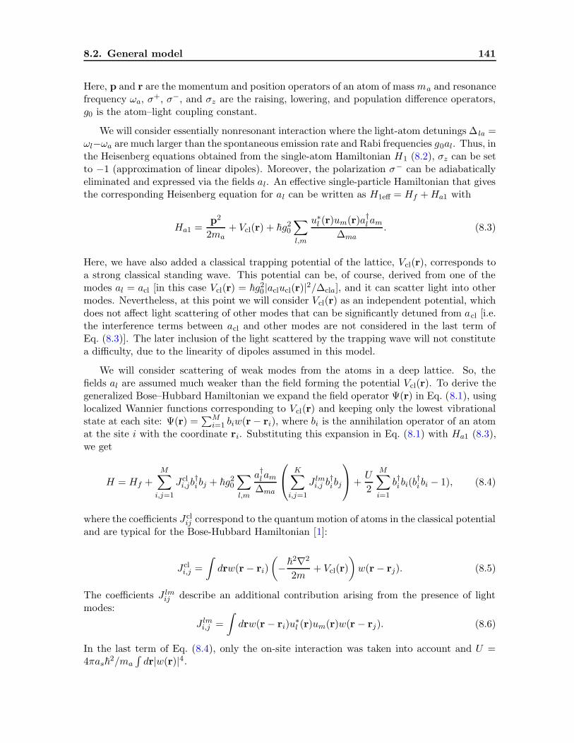
8.2. General model 141
Here, p and r are the momentum and position operators of an atom of mass ma and resonancefrequency ωa, σ
+, σ−, and σz are the raising, lowering, and population difference operators,g0 is the atom–light coupling constant.
We will consider essentially nonresonant interaction where the light-atom detunings ∆ la =ωl−ωa are much larger than the spontaneous emission rate and Rabi frequencies g0al. Thus, inthe Heisenberg equations obtained from the single-atom Hamiltonian H1 (8.2), σz can be setto −1 (approximation of linear dipoles). Moreover, the polarization σ− can be adiabaticallyeliminated and expressed via the fields al. An effective single-particle Hamiltonian that givesthe corresponding Heisenberg equation for al can be written as H1eff = Hf +Ha1 with
Ha1 =p2
2ma+ Vcl(r) + ~g2
0
∑
l,m
u∗l (r)um(r)a†l am∆ma
. (8.3)
Here, we have also added a classical trapping potential of the lattice, Vcl(r), corresponds toa strong classical standing wave. This potential can be, of course, derived from one of themodes al = acl [in this case Vcl(r) = ~g2
0 |aclucl(r)|2/∆cla], and it can scatter light into othermodes. Nevertheless, at this point we will consider Vcl(r) as an independent potential, whichdoes not affect light scattering of other modes that can be significantly detuned from acl [i.e.the interference terms between acl and other modes are not considered in the last term ofEq. (8.3)]. The later inclusion of the light scattered by the trapping wave will not constitutea difficulty, due to the linearity of dipoles assumed in this model.
We will consider scattering of weak modes from the atoms in a deep lattice. So, thefields al are assumed much weaker than the field forming the potential Vcl(r). To derive thegeneralized Bose–Hubbard Hamiltonian we expand the field operator Ψ(r) in Eq. (8.1), usinglocalized Wannier functions corresponding to Vcl(r) and keeping only the lowest vibrationalstate at each site: Ψ(r) =
∑Mi=1 biw(r− ri), where bi is the annihilation operator of an atom
at the site i with the coordinate ri. Substituting this expansion in Eq. (8.1) with Ha1 (8.3),we get
H = Hf +
M∑
i,j=1
Jcli,jb
†i bj + ~g2
0
∑
l,m
a†l am∆ma
K∑
i,j=1
J lmi,j b†ibj
+U
2
M∑
i=1
b†i bi(b†i bi − 1), (8.4)
where the coefficients J clij correspond to the quantum motion of atoms in the classical potential
and are typical for the Bose-Hubbard Hamiltonian [1]:
Jcli,j =
∫
drw(r− ri)
(
−~2∇2
2m+ Vcl(r)
)
w(r− rj). (8.5)
The coefficients J lmij describe an additional contribution arising from the presence of lightmodes:
J lmi,j =
∫
drw(r− ri)u∗l (r)um(r)w(r − rj). (8.6)
In the last term of Eq. (8.4), only the on-site interaction was taken into account and U =4πas~
2/ma
∫
dr|w(r)|4.
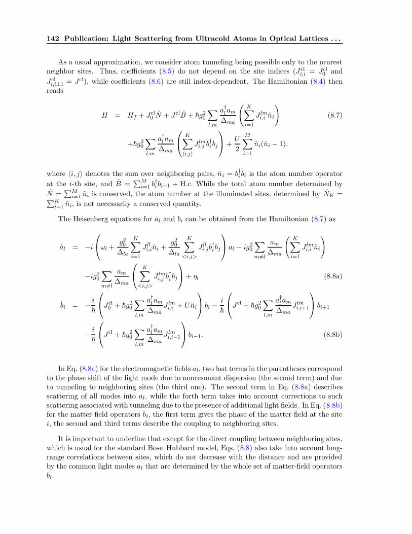
142 Publication: Light Scattering from Ultracold Atoms in Optical Lattices . . .
As a usual approximation, we consider atom tunneling being possible only to the nearestneighbor sites. Thus, coefficients (8.5) do not depend on the site indices (J cl
i,i = Jcl0 and
Jcli,i±1 = Jcl), while coefficients (8.6) are still index-dependent. The Hamiltonian (8.4) then
reads
H = Hf + Jcl0 N + JclB + ~g2
0
∑
l,m
a†lam∆ma
(
K∑
i=1
J lmi,i ni
)
(8.7)
+~g20
∑
l,m
a†l am∆ma
K∑
〈i,j〉J lmi,j b
†i bj
+U
2
M∑
i=1
ni(ni − 1),
where 〈i, j〉 denotes the sum over neighboring pairs, ni = b†ibi is the atom number operator
at the i-th site, and B =∑M
i=1 b†ibi+1 + H.c. While the total atom number determined by
N =∑M
i=1 ni is conserved, the atom number at the illuminated sites, determined by NK =∑K
i=1 ni, is not necessarily a conserved quantity.
The Heisenberg equations for al and bi can be obtained from the Hamiltonian (8.7) as
al = −i
ωl +g20
∆la
K∑
i=1
J lli,ini +g20
∆la
K∑
<i,j>
J lli,jb†ibj
al − ig20
∑
m6=l
am∆ma
(
K∑
i=1
J lmi,i ni
)
−ig20
∑
m6=l
am∆ma
K∑
<i,j>
J lmi,j b†i bj
+ ηl (8.8a)
bi = − i~
Jcl0 + ~g2
0
∑
l,m
a†l am∆ma
J lmi,i + Uni
bi −i
~
Jcl + ~g20
∑
l,m
a†lam∆ma
J lmi,i+1
bi+1
− i~
Jcl + ~g20
∑
l,m
a†l am∆ma
J lmi,i−1
bi−1. (8.8b)
In Eq. (8.8a) for the electromagnetic fields al, two last terms in the parentheses correspondto the phase shift of the light mode due to nonresonant dispersion (the second term) and dueto tunneling to neighboring sites (the third one). The second term in Eq. (8.8a) describesscattering of all modes into al, while the forth term takes into account corrections to suchscattering associated with tunneling due to the presence of additional light fields. In Eq. (8.8b)for the matter field operators bi, the first term gives the phase of the matter-field at the sitei, the second and third terms describe the coupling to neighboring sites.
It is important to underline that except for the direct coupling between neighboring sites,which is usual for the standard Bose–Hubbard model, Eqs. (8.8) also take into account long-range correlations between sites, which do not decrease with the distance and are providedby the common light modes al that are determined by the whole set of matter-field operatorsbi.

8.3. Scattering from a deep lattice and classical analogy 143
8.3 Scattering from a deep lattice and classical analogy
We will significantly reduce the general model described by the Hamiltonian (8.7) and Heisen-berg equations (8.8). In contrast to our previous paper [30] and works on so-called “Braggspectroscopy” [7–10], we will not consider excitations of the lattice by light and stimulationof matter waves. The focus of the present paper is a study of properties of light scatteredfrom the atoms in a prescribed quantum state, which is not necessarily the ground one. Themain result is the demonstration of the possibility to distinguish between different atomicquantum states of different statistics by measuring light only.
We consider a very deep lattice formed by a strong classical potential Vcl(r), so that theoverlap between Wannier functions in Eqs. (8.5) and (8.6) is small and tunneling betweenneighboring sites is impossible (J cl = 0 and J lmi,j = 0 for i 6= j). The on-site coefficients
J lmi,i (8.6) can be then approximated as J lmi,i = u∗l (ri)um(ri) neglecting details of the atomiclocalization, which are accessible even from the classical consideration [27–29].
For simplicity, we will consider scattering of a single classical mode a0 (“pump”) consid-ered as a given c-number quantity, into another mode a1 with the relaxation rate κ includedphenomenologically. The Heisenberg equation (8.8a) for the scattered light a1 then reads
a1 = −i[
ω1 +g20
∆1a
K∑
i=1
|u1(ri)|2ni]
a1 − ig20a0
∆0a
[
K∑
i=1
u∗1(ri)u0(ri)ni
]
− κa1 + η1, (8.9)
where we do not add the Langevin noise term, since we will be interested in normal orderedquantities only. In the Heisenberg equation for the matter–field operators bi (8.8b), only thefirst term is nonzero. This term affects only the phase of the matter field, but not the atomnumber operators ni = b†i bi. Hence, though the the matter–field phase still depends on thecommon light mode, the operators ni, appearing in Eq. (8.9), are constant in time.
We assume that the dispersion shift of the cavity mode g20/∆1a
∑Ki=1 |u1(ri)|2ni is much
smaller than κ or detuning between the pump and scattered light ∆01 = ω0 − ω1. Thus, astationary solution of Eq. (8.9) has a form
a1 = CD, C ≡ − ig20a0
∆0a(κ− i∆01), (8.10a)
D ≡K∑
i=1
u∗1(ri)u0(ri)ni, (8.10b)
where we have also assumed no additional pumping (η1 = 0) and replaced the operatorsa0,1(t) by their slowly varying envelopes a0,1(t) [a0,1(t) = a0,1 exp(−iω0t)] skipping in thefollowing notations all tilde signs.
This expressing the light operators in terms of the atomic ones in Eq. (8.10) is a centralresult here, which we will use to study the properties of the scattered field.
In the following, we will consider a 1D lattice of the period d with atoms trapped atxm = md (m = 1, 2, ..,M). The result for the field operator a1 (8.10a) with the operator D

144 Publication: Light Scattering from Ultracold Atoms in Optical Lattices . . .
(8.10b) has an analogy in classical diffraction. For scattering of a traveling wave a0 in thedirection of a traveling wave a1 from a lattice with 〈ni〉 = n at each site, the expectationvalue of the field is given by
〈a1〉 = C〈D〉 = C
K∑
m=1
eimδkxd〈nm〉 = Cnei(K+1)α−/2 sin (Kα−/2)
sin (α−/2), (8.11)
where α− = δkxd, and δkx = (k0−k1)x = k(sin θ0− sin θ1) is the projection of the differencebetween two wave vectors on the lattice direction, θ0,1 are the angles between wave vectorsand a vector normal to the lattice direction (cf. Fig. 8.1), k = ω/c for ω0 = ω1 = ω.
Equation (8.11) simply describes classical diffraction of the traveling wave a0 on a diffrac-tion grating formed by equally spaced atoms with positions of diffraction maxima and minima(i.e. scattering angles θ1) determined by the parameter α− depending on the geometry ofincident and scattered waves and diffraction grating through θ0, |k0,1|, and d. A more generalform of the operator D given by Eq. (8.10b) describes also diffraction of a standing wave a0
into another mode a1, which can be formed, for example, by a standing–wave or ring opticalcavity.
Equation (8.11) shows that the expectation value of the scattered field is sensitive onlyto the mean number of atoms per site n and reflects a direct analogy of light scatteringfrom a classical diffraction grating. Nevertheless, the photon number (intensity) and photonstatistics of the field a1 are sensitive to higher moments of the number operators ni as wellas to the quantum correlations between different lattice sites, which determines quantumstatistical properties of ultracold atoms in an optical lattice and will be considered in thenext sections.
8.4 Relation between quantum statistics of atoms and char-acteristics of scattered light
8.4.1 Probing quantum statistics by intensity and amplitude measure-ments
According to Eq. (8.10a), the expectation value of the photon number a†1a1 is proportional tothe expectation value of the operator D∗D. We introduce coefficients Ai(θ0, θ1) responsiblefor the geometry of the problem:
D =K∑
i=1
Aini, Ai(θ0, θ1) ≡ u∗1(ri)u0(ri),
A(θ0, θ1) ≡K∑
i=1
Ai(θ0, θ1), (8.12)
where u0,1(rm) = exp(imk0,1xd + φ0,1m) for traveling waves, and u0,1(rm) = cos(mk0,1xd +φ0,1m) for standing waves (m = 1, 2, ...M), k0,1x = |k0,1| sin θ0,1, θ0,1 are the angles between

8.4. Relation between quantum statistics of atoms and characteristics ofscattered light 145
mode wave vectors and a vector normal to the lattice axis; in the plane-wave approximation,additional phases φ0,1m are m-independent.
The expectation values of D and D∗D then read
〈D〉 =
K∑
i=1
Ai〈ni〉 = nA, (8.13a)
〈D∗D〉 =K∑
i,j=1
A∗iAj〈ninj〉 (8.13b)
= 〈nanb〉|A|2 + (〈n2〉 − 〈nanb〉)K∑
i=1
|Ai|2, (8.13c)
R(θ0, θ1) ≡ 〈D∗D〉 − |〈D〉|2
= (〈nanb〉 − n2)|A|2 + (〈n2〉 − 〈nanb〉)K∑
i=1
|Ai|2 (8.13d)
= 〈δnaδnb〉|A|2 + (〈δn2〉 − 〈δnaδnb〉)K∑
i=1
|Ai|2. (8.13e)
In Eqs. (8.13) we have used the following assumptions about the atomic quantum state |Ψ〉:(i) the expectation values of the atom number at all sites are the same, 〈ni〉 = n, (ii) thenonlocal pair correlations between atom numbers at different sites 〈ninj〉 are equal to eachother for any i 6= j and will be denoted as 〈nanb〉 (with a 6= b). The latter assumption isvalid for a deep lattice. We also introduced the fluctuation operators δni = ni − n, whichgives 〈δn2〉 equal to the variance (∆ni)
2 = 〈n2i 〉 − n2.
Equation (8.13a) reflects the fact that the expectation value of the field amplitude (8.10a)is sensitive only to the mean atom numbers and displays the angle dependence of classicaldiffraction given by the factor A(θ0, θ1), which depends on the mode angles and displayspronounced diffraction maxima and minima. Equation (8.13b) shows that the number ofscattered photons (intensity) at some angle is determined by the density–density correlations.In the simplest case of two traveling waves, the prefactors A∗
iAj = exp[iδkx(xj − xi)] withδkx = k0x − k1x. In this case, Eq. (8.13b) gives the so-called structure factor (function),which was considered in the works on light scattering from homogeneous BEC [17, 18]. Herewe essentially focus on optical lattices. Moreover, it will be shown, that the more generalEq. (8.13b), which includes scattering of standing waves, contains new measurable featuresdifferent from those of a usual structure factor.
Equation (8.13c) shows, that the angle dependence of the scattered intensity consists oftwo contributions. The first term has an angle dependence |A(θ0, θ1)|2 identical to that of theexpectation value of the field amplitude squared (8.13a). The second term is proportional tothe quantity 〈n2〉 − 〈nanb〉 giving quantum fluctuations and has a completely different angledependence
∑Ki=1 |Ai|2. The expression (8.13c) has a form similar to the one considered in
papers [13, 15, 16] on light scattering from a homogeneous BEC, where the scattered intensityconsisted of two parts: “coherent” (i.e. depending on the average density) and “incoherent”one (i.e. depending on the density fluctuations). Nevertheless, in the present case of a

146 Publication: Light Scattering from Ultracold Atoms in Optical Lattices . . .
periodic lattice, this similarity would be exact only in a particular case where there are nononlocal pair correlations 〈nanb〉 = nanb = n2 (〈δnaδnb〉 = 0), which in general is not trueand leads to observable difference between states with and without pair correlations.
Further insight into a physical role of nonlocal pair correlations can be obtained fromEqs. (8.13d) and (8.13e) for the “noise quantity” R(θ0, θ1) ≡ 〈D∗D〉 − |〈D〉|2, where wehave subtracted the classical (averaged) contribution |〈D〉|2 to the intensity 〈D∗D〉. Equa-tion (8.13e) shows that, in the noise quantity, a term with the classical angular distribution|A(θ0, θ1)|2 appears only if the pair correlations are nonzero. The physical meaning of thisresult is that, in an optical lattice, it is not only the density distribution that displays spatialperiodic structure leading to diffraction scattering, but also the distribution of number fluc-tuations themselves. In the framework of our assumption about equal pair correlations, thespatial distribution of fluctuations 〈δnaδnb〉 can be either the same as the density distribution(with a lattice period d) or zero. In the former case, pair correlations contribute to the firstterm in Eqs. (8.13d) and (8.13e) with classical distribution |A(θ0, θ1)|2, in the latter case,〈δnaδnb〉 = 0, and the only signal in the noise quantity is due to on-site fluctuations 〈δn2〉with a different angle dependence
∑Ki=1 |Ai|2. Note that, in general, the spatial distribution
of fluctuations can be different from that of the average density and can have a period propor-tional to the lattice period d. This will lead to additional peaks in the angular distribution ofthe noise quantity (8.13d), (8.13e). The generalization of those formulas is straightforward.
Even with spatially incoherent pump a0, the intensity of the scattered mode a†1a1 issensitive to the on-site atom statistics. To model this situation, the quantum expectationvalue 〈D∗D〉 (8.13b) should be additionally averaged over random phases φ0,1m appearing inthe definition of mode functions in Eq. (8.12). In Eq. (8.13b), only terms with i = j will thensurvive and the final result reads
〈D∗D〉inc = p0K〈n2〉, (8.14)
where p0 is equal to 1 for two traveling waves, 1/2 for a configuration with one standing wave,and 1/4, when both modes a0,1 are standing waves.
8.4.2 Quadrature measurements
The photon number a†1a1 is determined by the expectation value 〈D∗D〉, whereas 〈D〉 givesthe field 〈a1〉 (8.10a). While photon numbers can be directly measured, a field 〈a1〉 mea-surement requires a homodyne scheme. Such a measurement then makes 〈D〉 experimentallyaccessible. Actually for a quantum field only the expectation values of quadratures of a1
that are Hermitian operators and can be measured. Using Eq. (8.10a) and the commutation
relation [a1, a†1] = 1, the quadrature operator Xφ and its variance (∆Xφ)
2 can be written as
Xφ ≡ 1
2
(
a1e−iφ + a†1e
iφ)
= |C|XDφ−φC
, (8.15a)
X2φ =
1
4+ |C|2(XD
φ−φC)2, (8.15b)
(∆Xφ)2 ≡ 〈X2
φ〉 − 〈Xφ〉2 =1
4+ |C|2(∆XD
φ−φC)2, (8.15c)

8.4. Relation between quantum statistics of atoms and characteristics ofscattered light 147
where C = |C| exp(iφC) and the quadratures of D are
XDβ ≡ 1
2
(
De−iβ + D∗eiβ)
, (8.16a)
(∆XDβ )2 ≡ 〈(XD
β )2〉 − 〈XDβ 〉2. (8.16b)
In Eqs. (8.15), the phase φ is related to the homodyne reference phase, while φC is determinedby the phase of the pump a0 and parameters of the field–matter system [cf. Eq. (8.10a)].Hence, the phase β = φ − φC entering Eqs. (8.15) can be controlled by varying the phasedifference between the pump and homodyne fields.
Using Eq. (8.12), the quadrature operator XDβ reads
XDβ =
K∑
i=1
Aβi ni, Aβi (θ0, θ1) ≡ |Ai| cos (φAi− β),
Aβ(θ0, θ1) ≡K∑
i=1
Aβi (θ0, θ1), (8.17)
where Ai = |Ai| exp(iφAi), and we defined new quantities Aβi (θ0, θ1) and Aβ(θ0, θ1).
Since Eq. (8.17) for XDβ and Eq. (8.12) for D have a similar structure, the Eqs. (8.13) for
the quantities 〈D〉, 〈D∗D〉, and R can be rewritten for the quantities 〈XDβ 〉, 〈(XD
β )2〉, and
(∆XDβ )2, respectively, with the change of parameters Ai(θ0, θ1) and A(θ0, θ1) to Aβi (θ0, θ1)
and Aβ(θ0, θ1). Thus, the above discussion of Eqs. (8.13) can be repeated in terms of the
quadrature operators with the only difference that coefficients Aβi (θ0, θ1) and Aβ(θ0, θ1) now
depend also on the homodyne phase. An advantage of this reformulation is that the expec-tation value of the non-Hermitian operator a1, which determines 〈D〉, is now replaced bythe expectation value of the Hermitian operator Xφ, which is consistent with a procedure ofmeasuring quadratures of the quantum field a1.
8.4.3 Photon number fluctuations
While the intensity of the scattered light is sensitive to the second moments of the numberoperators ni, quantum statistics of the field reflexes the forth-order moments. The variance(∆nph)
2 of the photon number nph = a†1a1 is given by
(∆nph)2 = 〈n2ph〉 − 〈nph〉2 =: (∆n2
ph) : +〈nph〉 (8.18)
= |C|4(〈D∗2D2〉 − 〈D∗D〉2) + |C|2〈D∗D〉,
where : (∆n2ph) := 〈a†21 a2
1〉 − 〈a†1a1〉2 = |C|4(〈D∗2D2〉 − 〈D∗D〉2) is a normal ordered photon-number variance. Thus, the problem is reduced to measurements of the photon number
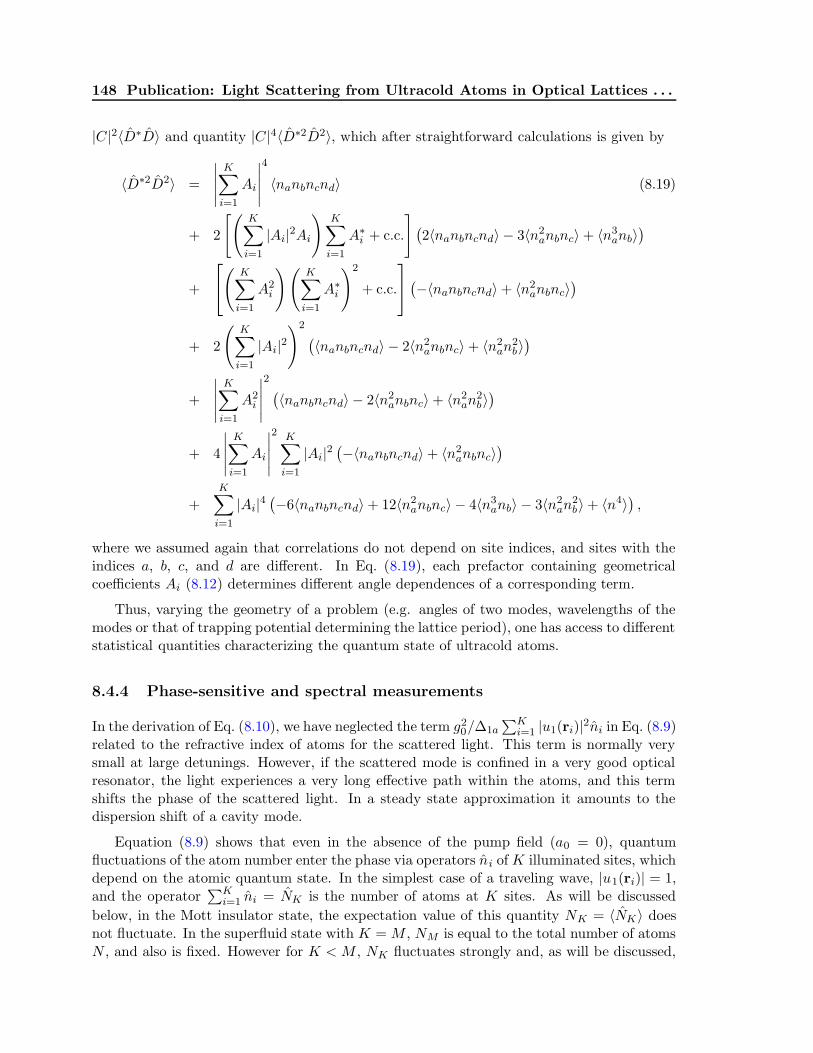
148 Publication: Light Scattering from Ultracold Atoms in Optical Lattices . . .
|C|2〈D∗D〉 and quantity |C|4〈D∗2D2〉, which after straightforward calculations is given by
〈D∗2D2〉 =
∣
∣
∣
∣
∣
K∑
i=1
Ai
∣
∣
∣
∣
∣
4
〈nanbncnd〉 (8.19)
+ 2
[(
K∑
i=1
|Ai|2Ai)
K∑
i=1
A∗i + c.c.
]
(
2〈nanbncnd〉 − 3〈n2anbnc〉+ 〈n3
anb〉)
+
(
K∑
i=1
A2i
)(
K∑
i=1
A∗i
)2
+ c.c.
(
−〈nanbncnd〉+ 〈n2anbnc〉
)
+ 2
(
K∑
i=1
|Ai|2)2(
〈nanbncnd〉 − 2〈n2anbnc〉+ 〈n2
an2b〉)
+
∣
∣
∣
∣
∣
K∑
i=1
A2i
∣
∣
∣
∣
∣
2(
〈nanbncnd〉 − 2〈n2anbnc〉+ 〈n2
an2b〉)
+ 4
∣
∣
∣
∣
∣
K∑
i=1
Ai
∣
∣
∣
∣
∣
2 K∑
i=1
|Ai|2(
−〈nanbncnd〉+ 〈n2anbnc〉
)
+
K∑
i=1
|Ai|4(
−6〈nanbncnd〉+ 12〈n2anbnc〉 − 4〈n3
anb〉 − 3〈n2an
2b〉+ 〈n4〉
)
,
where we assumed again that correlations do not depend on site indices, and sites with theindices a, b, c, and d are different. In Eq. (8.19), each prefactor containing geometricalcoefficients Ai (8.12) determines different angle dependences of a corresponding term.
Thus, varying the geometry of a problem (e.g. angles of two modes, wavelengths of themodes or that of trapping potential determining the lattice period), one has access to differentstatistical quantities characterizing the quantum state of ultracold atoms.
8.4.4 Phase-sensitive and spectral measurements
In the derivation of Eq. (8.10), we have neglected the term g20/∆1a
∑Ki=1 |u1(ri)|2ni in Eq. (8.9)
related to the refractive index of atoms for the scattered light. This term is normally verysmall at large detunings. However, if the scattered mode is confined in a very good opticalresonator, the light experiences a very long effective path within the atoms, and this termshifts the phase of the scattered light. In a steady state approximation it amounts to thedispersion shift of a cavity mode.
Equation (8.9) shows that even in the absence of the pump field (a0 = 0), quantumfluctuations of the atom number enter the phase via operators ni of K illuminated sites, whichdepend on the atomic quantum state. In the simplest case of a traveling wave, |u1(ri)| = 1,and the operator
∑Ki=1 ni = NK is the number of atoms at K sites. As will be discussed
below, in the Mott insulator state, the expectation value of this quantity NK = 〈NK〉 doesnot fluctuate. In the superfluid state with K = M , NM is equal to the total number of atomsN , and also is fixed. However for K < M , NK fluctuates strongly and, as will be discussed,

8.5. Quantum statistical properties of typical atomic distributions 149
for K M corresponds to a coherent state with 〈N2K〉 = 〈NK〉2 + 〈NK〉. Those statistical
properties of the atomic states are reflected in the phase of the light field. In particular,measurements of the dispersion shift of a cavity mode will show a frequency distributionreflecting the distribution of atom numbers.
This also opens an alternative spectral method of determining the quantum state of theatoms in a cavity with two degenerate modes. Let us consider the mode a0 as a dynamicalquantity obeying an equation as Eq. (8.9), which can be obtained from the set of Eq. (8.8a),while the second degenerate mode is called a1. The atoms lead to the collective normal-mode splitting of two cavity modes as recently experimentally observed [31]. If the couplingcoefficient between two degenerate modes, which is equal to g2
0/∆0aD [cf. Eq. (8.9) and thedefinition of the operator D in Eq. (8.12)], exceeds the cavity relaxation rate κ, a spectraldoublet instead of single maximum can be observed in the spectrum of the output light.
It is quite expected that the collective strong coupling between the modes and thusthe spectral splitting depends on the number of atoms in a lattice. Interestingly, from theequations for a0 and a1, it can be shown, that parameters of the normal-mode splitting(e.g. splitting frequency, linewidths) also depend on the atomic quantum state. So, spectralmode-splitting measurements also can be used to distinguish between atomic quantum phasesand allow a nondestructive measurement of a quantum phase transition dynamics. In thefollowing we will, however, restrict our study to single frequency measurements and leave amore detailed analysis of phase- and frequency-sensitive phenomena to other works [32].
8.5 Quantum statistical properties of typical atomic distribu-
tions
Let us briefly summarize some key statistical properties of typical states of N atoms atM lattice sites, i.e: the Mott insulator state (MI), superfluid state (SF), and a multisitecoherent-state approximation to the SF state.
The MI state represents a simple product of local Fock states at each site with preciselyni atoms at a site i. As a consequence, atom numbers at each site ni (as well as the numberof atoms at K sites NK) do not fluctuate, and there is no quantum correlations between sites:
|ΨMI〉 =
M∏
i=1
|ni〉i, (8.20a)
〈n2i 〉MI = n2
i , (8.20b)
(∆ni)2MI = 0, (8.20c)
〈N2K〉MI = N2
K , (8.20d)
(∆NK)2MI = 0, (8.20e)
〈nanb〉MI = nanb, (8.20f)
〈δnaδnb〉MI = 0, a 6= b. (8.20g)
Similarly to Eq. (8.20f),(8.20g), all two-, three-, and four-site quantities in Eq. (8.19) factorize.From the light–scattering point of view, this is the most classical atomic state, which corre-
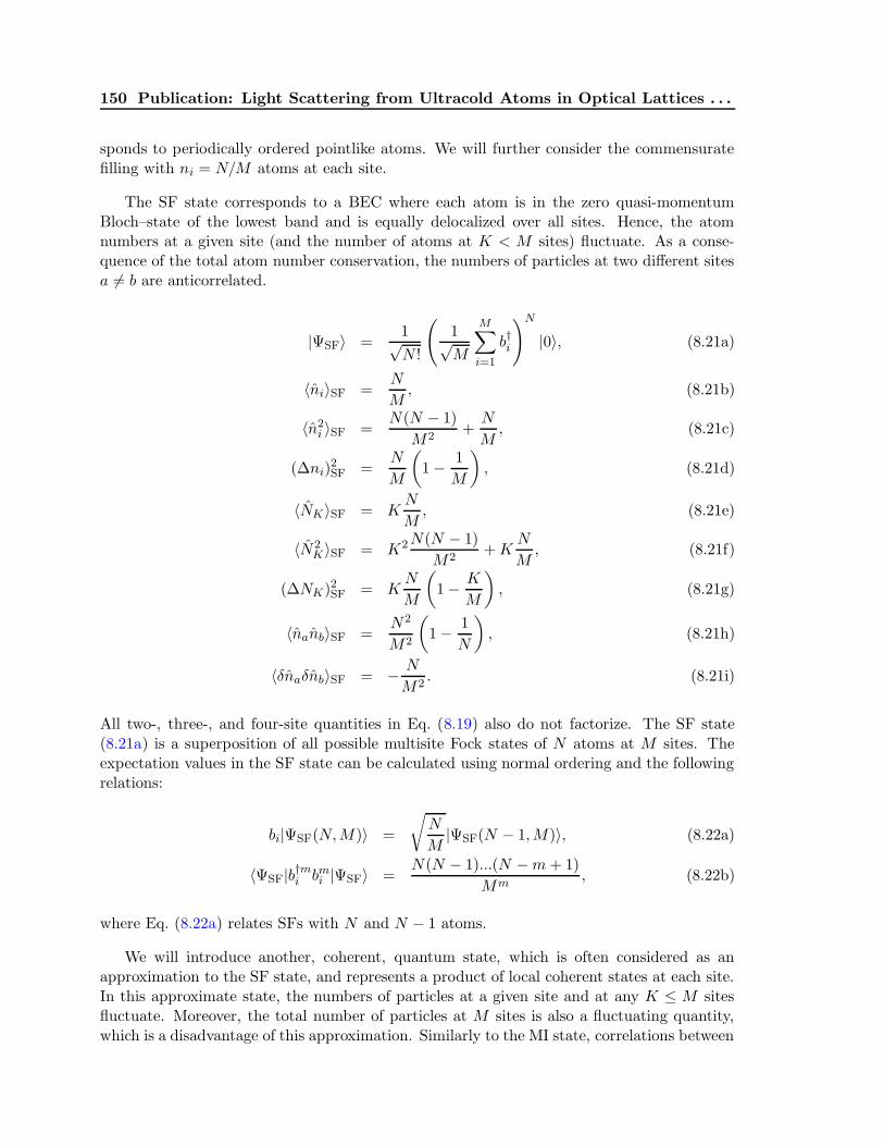
150 Publication: Light Scattering from Ultracold Atoms in Optical Lattices . . .
sponds to periodically ordered pointlike atoms. We will further consider the commensuratefilling with ni = N/M atoms at each site.
The SF state corresponds to a BEC where each atom is in the zero quasi-momentumBloch–state of the lowest band and is equally delocalized over all sites. Hence, the atomnumbers at a given site (and the number of atoms at K < M sites) fluctuate. As a conse-quence of the total atom number conservation, the numbers of particles at two different sitesa 6= b are anticorrelated.
|ΨSF〉 =1√N !
(
1√M
M∑
i=1
b†i
)N
|0〉, (8.21a)
〈ni〉SF =N
M, (8.21b)
〈n2i 〉SF =
N(N − 1)
M2+N
M, (8.21c)
(∆ni)2SF =
N
M
(
1− 1
M
)
, (8.21d)
〈NK〉SF = KN
M, (8.21e)
〈N2K〉SF = K2N(N − 1)
M2+K
N
M, (8.21f)
(∆NK)2SF = KN
M
(
1− K
M
)
, (8.21g)
〈nanb〉SF =N2
M2
(
1− 1
N
)
, (8.21h)
〈δnaδnb〉SF = − N
M2. (8.21i)
All two-, three-, and four-site quantities in Eq. (8.19) also do not factorize. The SF state(8.21a) is a superposition of all possible multisite Fock states of N atoms at M sites. Theexpectation values in the SF state can be calculated using normal ordering and the followingrelations:
bi|ΨSF(N,M)〉 =
√
N
M|ΨSF(N − 1,M)〉, (8.22a)
〈ΨSF|b†mi bmi |ΨSF〉 =N(N − 1)...(N −m+ 1)
Mm, (8.22b)
where Eq. (8.22a) relates SFs with N and N − 1 atoms.
We will introduce another, coherent, quantum state, which is often considered as anapproximation to the SF state, and represents a product of local coherent states at each site.In this approximate state, the numbers of particles at a given site and at any K ≤ M sitesfluctuate. Moreover, the total number of particles at M sites is also a fluctuating quantity,which is a disadvantage of this approximation. Similarly to the MI state, correlations between

8.5. Quantum statistical properties of typical atomic distributions 151
several different sites are absent.
|ΨCoh〉 = e−N/2M∏
i=1
e√N/Mb†i |0〉i, (8.23a)
〈ni〉Coh =N
M, (8.23b)
〈n2i 〉Coh =
N2
M2+N
M, (8.23c)
(∆ni)2Coh =
N
M, (8.23d)
〈NK〉Coh = KN
M, (8.23e)
〈N2K〉Coh = K2 N
2
M2+K
N
M, (8.23f)
(∆NK)2Coh = KN
M, (8.23g)
〈nanb〉Coh =N2
M2, (8.23h)
〈δnaδnb〉Coh = 0, (8.23i)
and we have
bi|ΨCoh(N,M)〉 =
√
N
M|ΨCoh(N,M)〉, (8.24a)
〈ΨCoh|b†mi bmi |ΨCoh〉 =Nm
Mm. (8.24b)
Comparing Eqs. (8.21), (8.22) for the SF state and Eqs. (8.23), (8.24) for the coherentone, we can state that under the approximation N,M → ∞, but finite N/M , the coherentstate is a good approximation for local one-site quantities and correlations between differentsites. Moreover, if K M , the SF expectation values related to the nonlocal NK operatorare also well approximated by corresponding quantities in the coherent state. Nevertheless,if the number of sites K is of the order of M , the coherent-state approximation fails for thosequantities.
One can prove even a more general statement for the functions 〈D∗D〉 (8.13) and 〈D∗2D2〉(8.19), which determine the intensity and statistics of light and are the most importantquantities in this work. If the number of sites illuminated by light, K, is much smaller thanthe total number of lattice sites M , the coherent-state is a good approximation for calculatingcharacteristics of scattered light in the limit N,M → ∞, but finite N/M . If, in opposite,the number of sites interacting with light is of the order of the total number of sites in thelattice, this approximation, in general, gives wrong results. As will be shown, it fails forlight scattering in the directions of diffraction maxima. The proof of the statement is basedon the consideration of the orders of sums in Eqs. (8.13), (8.19), which contain geometricalcoefficients Ai and are proportional to the powers of K, whereas factors containing atomfluctuations have powers of M in denominators.
Thus, light scattering from the region of a SF optical lattice with K M sites is equiv-alent to the light scattering from the atoms in the coherent state (in absolute values both

152 Publication: Light Scattering from Ultracold Atoms in Optical Lattices . . .
K and M can be very large). Moreover, in the directions outside diffraction maxima, thecoherent-state approximation works well even in the case where any number of sites is illu-minated.
In the following, discussing all states, we will use the notations n = N/M for the atomic“density” (expectation value of the particle number at each site) and NK = KN/M = nKfor the expectation value of the particle number at K sites. These two parameters fullycharacterize light scattering in the MI and coherent states, while all three parameters N ,M , and K are necessary to characterize scattering in the SF phase. For definitiveness, wewill discuss a case with large values of N , M , and K where difference between odd andeven number of lattice sites vanishes. Nevertheless, note that physical problems includingBECs with large atom number loaded into lattices with small site numbers are also of greatimportance [33, 34]. Results for this case, can be obtained from expressions of this sectionand Eqs. (8.13) and (8.19).
8.6 Example: 1D optical lattice in a transversally pumpedcavity
Before considering a general angular distribution of scattered light, we would like to presentthe most striking prediction of our model describing the difference between atomic quantumstates, observable by light scattering. Let us consider a configuration of Fig. 8.1 where thepump (traveling or standing wave) is orthogonal to the lattice (θ0 = 0), and the scatteredlight is collected along the lattice axis (θ1 = π/2) by a standing- or traveling-wave cavity.This geometry coincides with the one considered in the context of cavity cooling [35–37] andlattices in optical cavities [30]. Atoms are assumed to be trapped at each lattice site (d = λ/2)at field antinodes.
In this case, the operator D (8.12) is reduced to∑K
k=1(−1)k+1nk, which, independently on
an atomic state, gives zero for the expectation value of the field amplitude proportional to 〈D〉(here we assume even K). This corresponds to the classical destructive interference between
atoms separated by λ/2. In contrast, the photon number in a cavity a†1a1 is proportional to〈D∗D〉 = (〈n2〉 − 〈nanb〉)K [cf. Eq. (8.13c)], which is determined by statistics of a particularstate, and is equal to zero for the MI state and to NK for the SF state.
Thus, atoms in a MI state scatter no photons into a cavity, while a SF scatters numberof photons proportional to the atom number:
〈a1〉MI = 〈a1〉SF = 0, but 〈a†1a1〉MI = 0, 〈a†1a1〉SF = |C|2NK . (8.25)
Hence, already the mean photon number provides information about a quantum state ofultracold atoms.
The photon number fluctuations (∆nph)2 (8.18) are also different for various states. In
the MI state, the variance (∆|D|2)2 = 〈D∗2D2〉 − 〈D∗D〉2 is zero, (∆|D|2)2MI = 0, whereas inthe SF state, Eq. (8.19) gives a very strong noise (∆|D|2)2SF = 2N2
K (in highest order of NK).
Nonlinear light-matter dynamics in a cavity can lead to a new self-organized phase [36, 38]where all atoms occupy only each second site leading to doubling of the lattice period, d = λ.
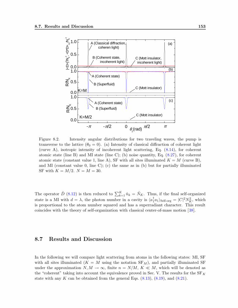
8.7. Results and Discussion 153
0.0
0.5
1.0
B (Coherent state, incoherent light)
C (Mott insulator, incoherent light)
A (Classical diffraction, coheren light)
(a)
0.0
0.5
1.0
ππ /20-π
/2-π
C (Mott insulator)
B (Superfluid)
A (Coherent state)
K=M/2
(c)
θ1(rad)
0.0
0.5
1.0
C (Mott insulator)B (Superfluid)
A (Coherent state)
K=M
|<D
>|2 /N
K2 , <D
*D> in
c/NK2
R/N
K(b)
R/N
K
Figure 8.2. Intensity angular distributions for two traveling waves, the pump istransverse to the lattice (θ0 = 0). (a) Intensity of classical diffraction of coherent light(curve A), isotropic intensity of incoherent light scattering, Eq. (8.14), for coherentatomic state (line B) and MI state (line C); (b) noise quantity, Eq. (8.27), for coherentatomic state (constant value 1, line A), SF with all sites illuminated K = M (curve B),and MI (constant value 0, line C); (c) the same as in (b) but for partially illuminatedSF with K = M/2. N = M = 30.
The operator D (8.12) is then reduced to∑K
k=1 nk = NK . Thus, if the final self-organized
state is a MI with d = λ, the photon number in a cavity is 〈a†1a1〉Self-org = |C|2N2K , which
is proportional to the atom number squared and has a superradiant character. This resultcoincides with the theory of self-organization with classical center-of-mass motion [38].
8.7 Results and Discussion
In the following we will compare light scattering from atoms in the following states: MI, SFwith all sites illuminated (K = M using the notation SFM ), and partially illuminated SFunder the approximation N,M → ∞, finite n = N/M , K M , which will be denoted asthe “coherent” taking into account the equivalence proved in Sec. V. The results for the SFK
state with any K can be obtained from the general Eqs. (8.13), (8.19), and (8.21).
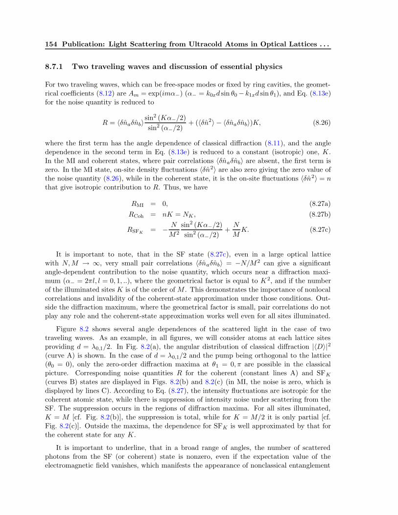
154 Publication: Light Scattering from Ultracold Atoms in Optical Lattices . . .
8.7.1 Two traveling waves and discussion of essential physics
For two traveling waves, which can be free-space modes or fixed by ring cavities, the geomet-rical coefficients (8.12) are Am = exp(imα−) (α− = k0xd sin θ0− k1xd sin θ1), and Eq. (8.13e)for the noise quantity is reduced to
R = 〈δnaδnb〉sin2 (Kα−/2)
sin2 (α−/2)+ (〈δn2〉 − 〈δnaδnb〉)K, (8.26)
where the first term has the angle dependence of classical diffraction (8.11), and the angledependence in the second term in Eq. (8.13e) is reduced to a constant (isotropic) one, K.In the MI and coherent states, where pair correlations 〈δnaδnb〉 are absent, the first term iszero. In the MI state, on-site density fluctuations 〈δn2〉 are also zero giving the zero value ofthe noise quantity (8.26), while in the coherent state, it is the on-site fluctuations 〈δn2〉 = nthat give isotropic contribution to R. Thus, we have
RMI = 0, (8.27a)
RCoh = nK = NK , (8.27b)
RSFK= − N
M2
sin2 (Kα−/2)
sin2 (α−/2)+N
MK. (8.27c)
It is important to note, that in the SF state (8.27c), even in a large optical latticewith N,M → ∞, very small pair correlations 〈δnaδnb〉 = −N/M 2 can give a significantangle-dependent contribution to the noise quantity, which occurs near a diffraction maxi-mum (α− = 2πl, l = 0, 1, ..), where the geometrical factor is equal to K 2, and if the numberof the illuminated sites K is of the order of M . This demonstrates the importance of nonlocalcorrelations and invalidity of the coherent-state approximation under those conditions. Out-side the diffraction maximum, where the geometrical factor is small, pair correlations do notplay any role and the coherent-state approximation works well even for all sites illuminated.
Figure 8.2 shows several angle dependences of the scattered light in the case of twotraveling waves. As an example, in all figures, we will consider atoms at each lattice sitesproviding d = λ0,1/2. In Fig. 8.2(a), the angular distribution of classical diffraction |〈D〉|2(curve A) is shown. In the case of d = λ0,1/2 and the pump being orthogonal to the lattice(θ0 = 0), only the zero-order diffraction maxima at θ1 = 0, π are possible in the classicalpicture. Corresponding noise quantities R for the coherent (constant lines A) and SFK
(curves B) states are displayed in Figs. 8.2(b) and 8.2(c) (in MI, the noise is zero, which isdisplayed by lines C). According to Eq. (8.27), the intensity fluctuations are isotropic for thecoherent atomic state, while there is suppression of intensity noise under scattering from theSF. The suppression occurs in the regions of diffraction maxima. For all sites illuminated,K = M [cf. Fig. 8.2(b)], the suppression is total, while for K = M/2 it is only partial [cf.Fig. 8.2(c)]. Outside the maxima, the dependence for SFK is well approximated by that forthe coherent state for any K.
It is important to underline, that in a broad range of angles, the number of scatteredphotons from the SF (or coherent) state is nonzero, even if the expectation value of theelectromagnetic field vanishes, which manifests the appearance of nonclassical entanglement

8.7. Results and Discussion 155
between the light and manybody atomic system. Moreover, in contrast to MI state, atomsin SF state scatter photons at angles, where the classical diffraction does not exist.
For example, in a simple configuration considered in Sec. VI where the pump is orthogonalto the lattices (θ0 = 0), and the scattered light is collected by a cavity along the lattice axis(θ1 = π/2), the atoms in the MI state scatter no photons as in classical diffraction minimum.
In contrast, atoms in the SFK state scatter the number of photons a†1a1 = |C|2〈D∗D〉 =|C|2NK , proportional to the number of the atoms illuminated [cf. Eq. (8.27) and Fig. 8.2(b)at the angle θ1 = π/2].
For two traveling waves, the expression for D (8.12), in a diffraction maximum where allatoms radiate in phase with each other and α− = 2πl, is reduced to the operator NK . Thus,the quantity 〈D〉 = NK = nK is the expectation value of the atom number at K sites andproportional to the average atom number at a single site. The intensity of the light scatteredinto a diffraction maximum is determined by 〈D∗D〉 = 〈N2
K〉, while noise R = (∆NK)2 givesthe atom number variance at K sites. The latter statement corresponds to Figs. 8.2(b) and8.2(c) displaying the total noise suppression in SFM state, where the total atom number atall sites K = M does not fluctuate, while for K < M , NK is a fluctuating quantity and thenoise suppression is only partial.
At the angle of a classical diffraction “minimum” (forK 1 this is approximately valid forany angle outside narrow regions of maxima), the expectation value of the field amplitude iszero, as well as the first terms in Eqs. (8.13c), (8.13d), (8.13e), and both the intensity 〈D∗D〉and noise R are proportional to the quantity 〈n2〉 − 〈nanb〉 giving the difference betweenlocal and nonlocal fluctuations. For two traveling waves, the coefficient of proportionality isisotropic and equal to K [cf. Eq. (8.26)].
For scattering of incoherent light (8.14), the intensity is proportional to the local quantity〈n2〉 and is shown in Fig. 8.2(a) for MI (curve C) and coherent, almost the same as in SF,(curve B) states. This quantity can be also obtained under coherent scattering of two travelingwaves, if one tunes the angles such that the geometrical factor of the first term in Eq. (8.26)is equal to K. Practically, this variant is easy to achieve only for a diffraction pattern withdiffraction maxima, which are not too narrow.
Hence, in an optical experiment, both global statistical quantities related to K ≤M sites,local quantities reflecting statistics at a single site, and pair correlations can be obtained. Itis important, that local statistics can be determined by global measurements, i.e., an opticalaccess to a single site is not necessary.
Therefore, light scattering gives a possibility to distinguish different quantum states ofultracold atoms. As demonstrated by Eq. (8.27) and Fig. 8.2, MI and SFM states are dis-tinguishable in diffraction “minima” and in incoherent light, while they are indistinguishable(for traveling waves) in maxima, because the total atom number contributing to the maxi-mum does not fluctuate. The SFM and coherent states can be distinguished in diffractionmaxima only. The MI and coherent states can be distinguished in any angle of the scatteringpattern.
Measurements of the noise quantity discussed or, alternatively, related quantities forquadratures (8.16) or photon number variance (8.18), give the values, which are differentin orders of the emitter number NK for different quantum states. Nevertheless, for large NK ,
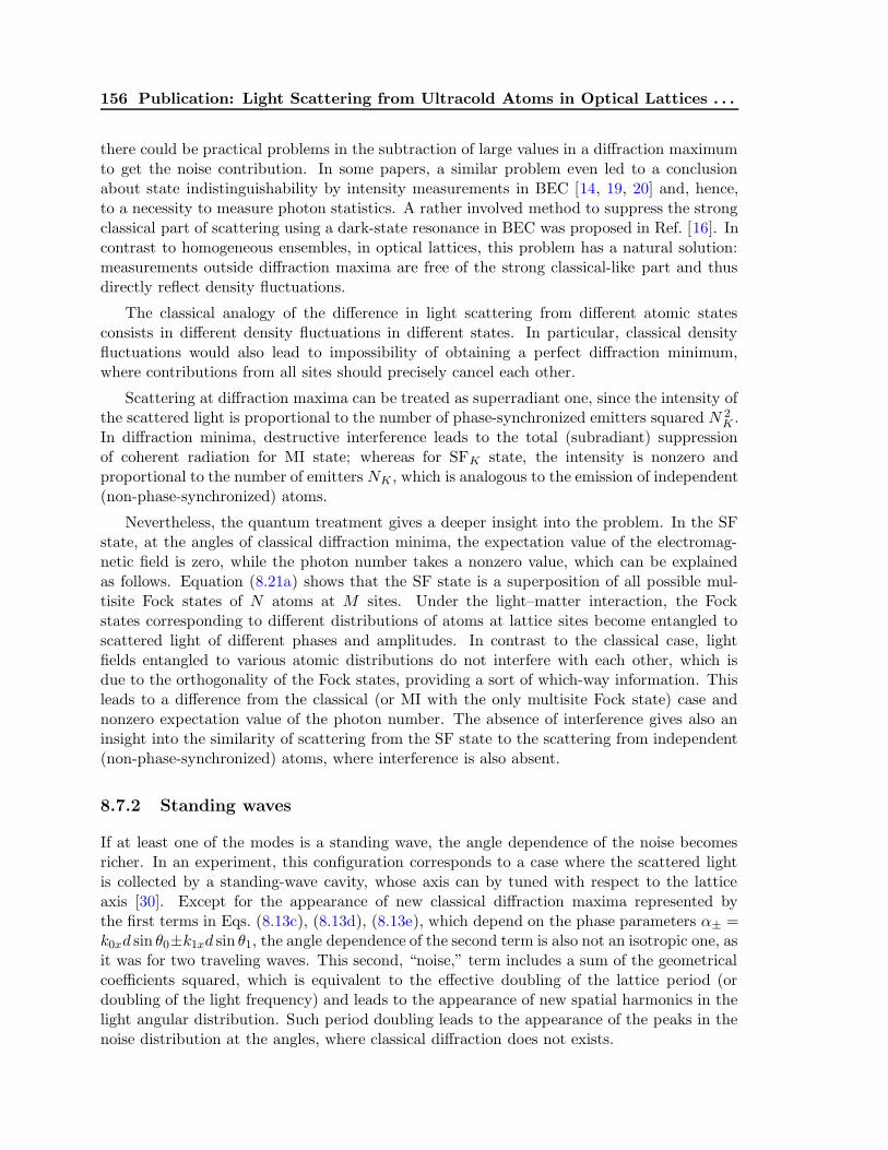
156 Publication: Light Scattering from Ultracold Atoms in Optical Lattices . . .
there could be practical problems in the subtraction of large values in a diffraction maximumto get the noise contribution. In some papers, a similar problem even led to a conclusionabout state indistinguishability by intensity measurements in BEC [14, 19, 20] and, hence,to a necessity to measure photon statistics. A rather involved method to suppress the strongclassical part of scattering using a dark-state resonance in BEC was proposed in Ref. [16]. Incontrast to homogeneous ensembles, in optical lattices, this problem has a natural solution:measurements outside diffraction maxima are free of the strong classical-like part and thusdirectly reflect density fluctuations.
The classical analogy of the difference in light scattering from different atomic statesconsists in different density fluctuations in different states. In particular, classical densityfluctuations would also lead to impossibility of obtaining a perfect diffraction minimum,where contributions from all sites should precisely cancel each other.
Scattering at diffraction maxima can be treated as superradiant one, since the intensity ofthe scattered light is proportional to the number of phase-synchronized emitters squared N 2
K .In diffraction minima, destructive interference leads to the total (subradiant) suppressionof coherent radiation for MI state; whereas for SFK state, the intensity is nonzero andproportional to the number of emitters NK , which is analogous to the emission of independent(non-phase-synchronized) atoms.
Nevertheless, the quantum treatment gives a deeper insight into the problem. In the SFstate, at the angles of classical diffraction minima, the expectation value of the electromag-netic field is zero, while the photon number takes a nonzero value, which can be explainedas follows. Equation (8.21a) shows that the SF state is a superposition of all possible mul-tisite Fock states of N atoms at M sites. Under the light–matter interaction, the Fockstates corresponding to different distributions of atoms at lattice sites become entangled toscattered light of different phases and amplitudes. In contrast to the classical case, lightfields entangled to various atomic distributions do not interfere with each other, which isdue to the orthogonality of the Fock states, providing a sort of which-way information. Thisleads to a difference from the classical (or MI with the only multisite Fock state) case andnonzero expectation value of the photon number. The absence of interference gives also aninsight into the similarity of scattering from the SF state to the scattering from independent(non-phase-synchronized) atoms, where interference is also absent.
8.7.2 Standing waves
If at least one of the modes is a standing wave, the angle dependence of the noise becomesricher. In an experiment, this configuration corresponds to a case where the scattered lightis collected by a standing-wave cavity, whose axis can by tuned with respect to the latticeaxis [30]. Except for the appearance of new classical diffraction maxima represented bythe first terms in Eqs. (8.13c), (8.13d), (8.13e), which depend on the phase parameters α± =k0xd sin θ0±k1xd sin θ1, the angle dependence of the second term is also not an isotropic one, asit was for two traveling waves. This second, “noise,” term includes a sum of the geometricalcoefficients squared, which is equivalent to the effective doubling of the lattice period (ordoubling of the light frequency) and leads to the appearance of new spatial harmonics in thelight angular distribution. Such period doubling leads to the appearance of the peaks in thenoise distribution at the angles, where classical diffraction does not exists.
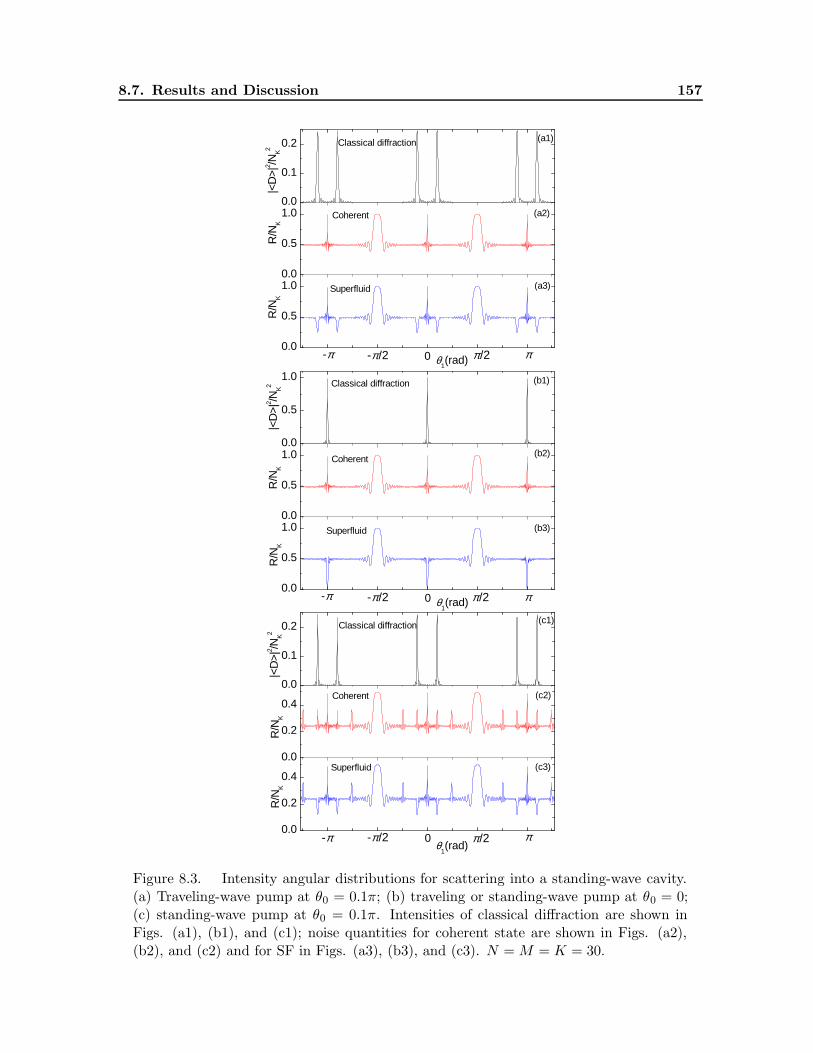
8.7. Results and Discussion 157
0.0
0.1
0.2 Classical diffraction
(a1)
0.0
0.5
1.0
-π /2
-π /2-π
-π /2-π
Superfluid (a3)
θ1(rad)
0.0
0.5
1.0
R/N
KR
/NK
Coherent
|<D
>|2 /N
K2
(a2)
0.0
0.5
1.0
ππ /20
ππ /20
ππ /20
Classical diffraction
(b1)
0.0
0.5
1.0
R/N
KR
/NK
Coherent
|<D
>|2 /N
K2
(b2)
0.0
0.5
1.0
θ1(rad)
Superfluid (b3)
0.0
0.1
0.2 Classical diffraction
(c1)
0.0
0.2
0.4
R/N
KR
/NK
Coherent
|<D
>|2 /N
K2
(c2)
0.0
0.2
0.4
-π
Superfluid (c3)
θ1(rad)
Figure 8.3. Intensity angular distributions for scattering into a standing-wave cavity.(a) Traveling-wave pump at θ0 = 0.1π; (b) traveling or standing-wave pump at θ0 = 0;(c) standing-wave pump at θ0 = 0.1π. Intensities of classical diffraction are shown inFigs. (a1), (b1), and (c1); noise quantities for coherent state are shown in Figs. (a2),(b2), and (c2) and for SF in Figs. (a3), (b3), and (c3). N = M = K = 30.
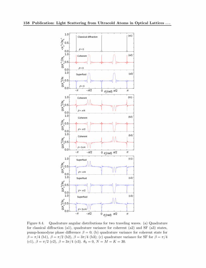
158 Publication: Light Scattering from Ultracold Atoms in Optical Lattices . . .
0.0
0.5
1.0Classical diffraction
β = 0
(a1)
0.0
0.5
1.0
-π /2-π
-π /2-π
-π /2-π
Superfluid
β = 0
(a3)
θ1(rad)
0.0
0.5
1.0Coherent
β = 0
(∆X
βD )2 /N( ∆
XβD )2 /N
K<X
βD >2 /NK2
(a2)
0.0
0.5
1.0
ππ /20
ππ /20
ππ /20
Coherent
β = π /4
(b1)
0.0
0.5
1.0Coherent
(∆X
βD )2 /NK
(∆X
βD )2 /NK
(∆X
βD )2 /NK
β = π /2
(b2)
0.0
0.5
1.0
Coherent
β = 3π /4
(b3)
θ1(rad)
0.0
0.5
1.0 Superfluid
β = π /4
(c1)
0.0
0.5
1.0 Superfluid
(∆X
βD )2 /NK
(∆X
βD )2 /NK
(∆X
βD )2 /NK
β = π /2
(c2)
0.0
0.5
1.0 Superfluid
β = 3π /4
(c3)
θ1(rad)
Figure 8.4. Quadrature angular distributions for two traveling waves. (a) Quadraturefor classical diffraction (a1), quadrature variance for coherent (a2) and SF (a3) states,pump-homodyne phase difference β = 0; (b) quadrature variance for coherent state forβ = π/4 (b1), β = π/2 (b2), β = 3π/4 (b3); (c) quadrature variance for SF for β = π/4(c1), β = π/2 (c2), β = 3π/4 (c3). θ0 = 0, N = M = K = 30.
8.7. Results and Discussion 159
In Fig. 8.3(a), angular distributions of the scattered light are shown for a traveling-wavepump, which is almost orthogonal to a lattice (θ0 = 0.1π), while the probe is a standing wave.Classical diffraction pattern [cf. Fig. 8.3(a1)] is determined by |A|2 through the parametersα± and shows zero-order diffraction maxima in transmission (θ1 = θ0 and its counterpart dueto the presence of the standing-wave cavity at θ1 = π + θ0) and reflection (θ1 = π − θ0 andthe counterpart at −θ0). The intensity noise for atoms in the coherent state [cf. Fig. 8.3(a2)]is determined by
∑Ki=1 |Ai|2 through another parameter 2α1 = 2k1xd sin θ1 and has different
characteristic features at θ1 = 0, π, and ±π/2. It is the latter feature that corresponds tothe effective frequency doubling and appears at an angle, where classical diffraction has aminimum. In the case of SFM state [cf. Fig. 8.3(a3)], pair correlations in Eqs. (8.13d) and(8.13e) are nonzero, hence, both geometrical factors contribute to the noise distribution, whichhas the features at angles characteristic to both classical scattering and the light noise of thecoherent-state case. Outside the characteristic features, the noise distribution is isotropic andtakes a nonzero value similar to the case of two traveling waves [cf. Fig. 8.2]. Figure 8.3(b)shows a simpler situation, where the pump is precisely orthogonal to the lattices (θ0 = 0).
In Fig. 8.3(c), a situation similar to Fig. 8.3(a) is shown for the case where both the pumpand probe are standing waves. While classical diffraction still depends on the parameters α±,the factor
∑Ki=1 |Ai|2 determining the intensity noise depends on four parameters 2α0,1 =
2k0,1xd sin θ0,1 and 2α±. Thus, in the light noise from a lattice in the coherent and SFstates, the features are placed at the positions of classical zero-order diffraction maximaand the angles, which would correspond to the classical scattering from a lattice with adoubled period d = λ, where the appearance of first-order diffraction maxima is possible.Similar to Fig. 8.3(a), features at θ1 = 0, π, and π/2 also exist. In the case θ0 = 0, theangular distribution for two standing waves is identical to that of one standing wave shownin Fig. 8.3(b).
In the SFM state, there are two types of diffraction maxima. In the first one, the noise canbe completely suppressed due to the total atom number conservation, similarly to the caseof traveling waves. This occurs, if the condition of the maximum is fulfilled for both of twotraveling waves forming a single standing wave [cf. Fig. 8.3(b)]. In the second type, even forK = M , only partial noise suppression is possible, since only one of the traveling waves is ina maximum, while another one, being in a minimum, produces the noise [cf. Figs. 8.3(a) and8.3(c)]. In contrast to two traveling modes, in the second type of maxima, one can distinguishbetween SFM and MI states, since MI produces no noise in any direction.
8.7.3 Quadratures and photon statistics
An analysis of the angular distribution of the quadrature variance (∆XDβ )2 (8.16b) shows,
that even for two traveling waves, new peaks due to effective period doubling appear [seeFig. 8.4(a)]. Additionally, the amplitude of noise features can be varied by the phase differencebetween the pump and homodyne beams β, which is shown in Figs. 8.4(b) for the coherentand in Fig. 8.4(c) SFM states. In the coherent state, all peaks are very sensitive to β. Inthe SFM state, the noise suppression at diffraction maxima is insensitive to variations of β,whereas other peaks are β-dependent. The relation of (∆XD
β )2 to the quadrature variance ofthe light field is given by Eq. (8.15c).

160 Publication: Light Scattering from Ultracold Atoms in Optical Lattices . . .
0.0
0.5
1.0
C (Mott insulator, incoherent light)
B (Coherent state, incoherent light)
A (Classical diffraction, coheren light)
(a)
0.0
0.2
0.4
ππ /20-π
/2-π
C (Superfluid, incoherent light)
A (Superfluid, coherent light)
D (MI, incoherent light)
B (Coherent state, incoherent light)
(c)
θ1(rad)
0.0
0.5
1.0
B (Coherent state, incoherent light)
A (Coherent state, coherent light)
(∆|D
|2 )2 (10
4 )
(∆
|D|2 )2 (
10 5 )
|<D
>|2 /N
K2 , <D
*D> in
c/NK2
(b)
Figure 8.5. Angular distributions of photon-number variances for two traveling waves.(a) Intensity of classical diffraction (curve A), isotropic intensity of incoherent lightscattering, Eq. (8.14), for coherent atomic state (line B) and MI state (line C); (b)normal ordered photon-number variance for coherent atomic state under scattering ofcoherent, Eq. (8.28) (curve A), and incoherent (line B) light; (c) normal ordered photon-number variance for SF state under scattering of coherent, Eq. (8.28) (curve A), andincoherent (line C) light, variance for coherent (line B) and MI (curve D) states underscattering of incoherent light. Normal ordered photon-number variance for MI stateunder scattering of coherent light is zero for all angles. θ0 = 0, N = M = K = 30.

8.8. Conclusions 161
The angle dependence of the variance (∆|D|2)2 = 〈D∗2D2〉 − 〈D∗D〉2, which is pro-portional to the normal ordered photon-number variance and determines the light statistics(8.18), also shows anisotropic features due to frequency doubling even for two traveling waves(Fig. 8.5). In this case, Eq. (8.19) is reduced to
〈D∗2D2〉 =
(
sin(Kα−/2)sin(α−/2)
)4
〈nanbncnd〉 (8.28)
+ 2
(
sin(Kα−/2)sin(α−/2)
)3 cos(Kα−/2)cos(α−/2)
(
〈n2anbnc〉 − 〈nanbncnd〉
)
− 4
(
sin(Kα−/2)sin(α−/2)
)2[
(K − 2)〈nanbncnd〉 − (K − 3)〈n2anbnc〉 − 〈n3
anb〉]
+
(
sinKα−sinα−
)2(
〈nanbncnd〉 − 2〈n2anbnc〉+ 〈n2
an2b〉)
+ 2K2(
〈nanbncnd〉 − 2〈n2anbnc〉+ 〈n2
an2b〉)
+ K(
−6〈nanbncnd〉+ 12〈n2anbnc〉 − 4〈n3
anb〉 − 3〈n2an
2b〉+ 〈n4〉
)
,
where the first four terms has features at angles typical to classical diffraction, the fourthterm is also responsible for the doubled-frequency feature, and the last two terms contributeto the isotropic component.
For the coherent state, the light scattered into a diffraction maximum displays a verystrong noise (equal to 4N 3
K + 6N2K + Nk because 〈D∗2D2〉 = N4
K + 6N3K + 7N2
K + Nk and
〈D∗D〉 = N2K +NK), which is much stronger than the isotropic component (N 2
K in highestorder of NK) and the features at θ1 = ±π/2 (2N 2
K in highest order of NK) [Fig. 8.5(b)]. InSFM state, the noise at maxima can be suppressed, while at other angles, in highest order ofNK , it is equal to that of the coherent state [Fig.8.5(c)]. In MI state, the variance (∆|D|2)2is zero for all angles. Conclusions about state distinguishing by measuring light statisticsare very similar to those drown from the intensity and amplitude measurements, which havebeen discussed in Sec. VIIA, including scattering of incoherent light (see Fig. 8.5 and thediscussion of Fig. 8.2).
In experiments, the nontrivial angle dependence of the noise can help in the separationof the light noise reflecting atom statistics from technical imperfections.
8.8 Conclusions
We studied off-resonant collective light scattering from ultracold atoms trapped in an opticallattice. Measuring the light field allows to characterize the quantum state of atoms in anondestructive way and in particular distinguish between different atomic states. The scat-tered light differs in intensity, quadrature variances, and photon statistics. A measurementof the intensity angular distribution provides information about atom number fluctuationsin a finite lattice region, local quantum statistics at single sites, and pair correlations. Notethat even local statistics can be determined by global measurements without an optical ac-cess to particular sites. Alternatively to angle-resolved measurements, variations of the modewavelengths with respect to the wavelength of a trapping beam can be considered.
162 Publication: Light Scattering from Ultracold Atoms in Optical Lattices . . .
Light scattering as a diagnostic tool has particular advantages for optical lattices in con-trast to scattering from a homogeneous BEC. Here one has a natural way to suppress thestrong classical scattering background by looking at the directions of diffraction minima. Inthese directions the expectation value of the field amplitude vanishes while the intensity (pho-ton number) is nonzero and directly reflects quantum fluctuations. Furthermore, in an opticallattice, the signal is sensitive not only to the periodic density distribution, but also to theperiodic density fluctuations, giving an access to even very small nonlocal pair correlations.These can be obtained by measuring light at diffraction maxima.
As the most striking example, we considered light scattering from a 1D lattice in atransversally pumped optical cavity as in a setup involving collective cavity cooling [36, 38–40]. The number of photons scattered into the cavity is zero for the Mott insulator phase butproportional to the atom number in the superfluid phase. Both states have almost the sameaverage density but different quantum uncertainties. So the superfluid state is a quantumsuperposition of different Fock states corresponding to all possible distributions of N atomsat M sites. Under illumination by a coherent light, various Fock states become entangled toscattered light states with different amplitudes and phases. In contrast to classical scatter-ing, where the atoms are described by c-number center-of-mass positions [41], for a quantumdescription of the atomic motion the light field amplitudes corresponding to different atomicdistributions do not interfere. This is due to the orthogonality of Fock states forming thesuperfluid providing a sort of which way information.
In the example configuration, the cavity-field amplitude is determined by the atom numberoperators ni = b†i bi. Hence, the expectation value of the field amplitude is sensitive to theaverage density only. In contrast, the intracavity photon number reflects the second momentsof atom number operators (e.g. density-density correlations), while photon statistics reflectsthe forth moments.
Let’s emphasize that other physical systems are possible, where the light amplitude de-pends on the matter-field amplitudes bi, while the intensity is sensitive to density operatorsni. The latter situation is typical to configurations, where two or more atomic subsystemsexist and can interact with each other, in particular, through light fields. The examplesare matter-wave superradiance and amplification, where two or more momentum states ofcold atoms were observed [11, 12, 42, 43], and interaction between two BECs with differentinternal [44–47] or motional [48] atomic states. In the framework of our paper, matter-fieldamplitudes bi can also contribute to light amplitudes al, if the tunneling between lattice sitesis important, which we have considered in the general model in Sec. II. In the rest of thepaper, the lattice was assumed deep leading to negligible tunneling.
In general, a variety of optical effects can be sensitive to a quantum state of an ultracoldmatter, if the density operators enter measurable quantities nonlinearly, such that the ex-pectation value of those quantities cannot be simply expressed through expectation values ofdensity operators. For instance, the χ(3) nonlinearity [49] and refractive index of a gas, wherenonlocal field effects are important [50], were shown to depend on atom statistics. In thispaper, we focused on such nonlinear quantities as intensity, quadrature variances, and pho-ton statistics of scattered light [51]. Phase-sensitive and spectral characteristics mentionedin Sec. IV.D reflect the dependence of the dispersion of a medium on the quantum state ofmatter [32, 52]. Moreover, such dispersion effects (e.g. cavity-mode shift) will reflect atomstatistics not only in light intensity, but even in light amplitudes 〈al〉.
BIBLIOGRAPHY 163
So far we have neglected the dynamic back action of scattered field on atoms. This can bewell justified in a deep lattice where the momentum transfer is by far not enough to changethe atomic vibrational state as long as not too many photons are scattered. Even withoutenergy transfer the information one gets from the light will induce measurement back-action.This should have intriguing consequences for multiple consecutive measurements on the lightscattered from optical lattices.
Acknowledgments
This work was supported by the Austrian Science Fund FWF (grants P17709 and S1512).
Bibliography
[1] D. Jaksch, C. Bruder, J. I. Cirac, C. W. Gardiner, and P. Zoller, Phys. Rev. Lett. 81,3108 (1998).
[2] M. Greiner, O. Mandel, T. Esslinger, T. Hansch, and I. Bloch, Nature 415, 39 (2002).
[3] S. Folling, F. Gerbier, A. Widera, O. Mandel, T. Gericke, and I. Bloch, Nature 434, 481(2005).
[4] E. Altman, E. Demler, and M. D. Lukin, Phys. Rev. A 70, 013603 (2004).
[5] J. Stenger, S. Inouye, A. P. Chikkatur, D. M. Stamper-Kurn, D. E. Pritchard, andW. Ketterle, Phys. Rev. Lett. 82, 4569 (1999).
[6] P. B. Blakie, R. J. Ballagh, and C. W. Gardiner, Phys. Rev. A 65, 033602 (2002).
[7] R. Roth and K. Burnett, Phys. Rev. A 68, 023604 (2003).
[8] T. Stoferle, H. Moritz, C. Schori, M. Kohl, and T. Esslinger, Phys. Rev. Lett. 92, 130403(2004).
[9] C. Menotti, M. Kramer, L. Pitaevskii, and S. Stringari, Phys. Rev. A 67, 053609 (2003).
[10] A. M. Rey, P. B. Blakie, G. Pupillo, C. J. Williams, and C. W. Clark, Phys. Rev. A 72,023407 (2005).
[11] M. G. Moore, O. Zobay, and P. Meystre, Phys. Rev. A 60, 1491 (1999).
[12] H. Pu, W. Zhang, and P. Meystre, Phys. Rev. Lett. 91, 150407 (2003).
[13] L. You, M. Lewenstein, and J. Cooper, Phys. Rev. A 51, 4712 (1995).
[14] Z. Idziaszek, K. Rzazewski, and M. Lewenstein, Phys. Rev. A 61, 053608 (2000).
[15] O. E. Mustecaplioglu and L. You, Phys. Rev. A 62, 063615 (2000).
[16] O. E. Mustecaplioglu and L. You, Phys. Rev. A 64, 033612 (2001).
164 Publication: Light Scattering from Ultracold Atoms in Optical Lattices . . .
[17] J. Javanainen, Phys. Rev. Lett. 75, 1927 (1995).
[18] J. Javanainen and J. Ruostekoski, Phys. Rev. A 52, 3033 (1995).
[19] J. I. Cirac, M. Lewenstein, and P. Zoller, Phys. Rev. Lett. 72, 2977 (1994).
[20] J. I. Cirac, M. Lewenstein, and P. Zoller, Phys. Rev. A 50, 3409 (1994).
[21] H. Saito and M. Ueda, Phys. Rev. A 60, 3990 (1999).
[22] G. A. Prataviera and M. C. de Oliveira, Phys. Rev. A 70, 011602(R) (2004).
[23] J. Javanainen and J. Ruostekoski, Phys. Rev. Lett. 91, 150404 (2003).
[24] I. B. Mekhov, C. Maschler, and H. Ritsch, quant-ph/0610073, to be published in Phys.Rev. Lett.
[25] T. Bourdel, T. Donner, S. Ritter, A. Ottl, M. Kohl, and T. Esslinger, Phys. Rev. A 73,043602 (2006).
[26] I. Teper, Y. J. Lin, and V. Vuletic, Phys. Rev. Lett. 97, 023002 (2006).
[27] G. Birkl, M. Gatzke, I. H. Deutsch, S. L. Rolston, and W. D. Phillips, Phys. Rev. Lett.75, 2823 (1995).
[28] M. Weidemuller, A. Hemmerich, A. Gorlitz, T. Esslinger, and T. W. Hansch, Phys. Rev.Lett. 75, 4583 (1995).
[29] S. Slama, C. von Cube, M. Kohler, C. Zimmermann, and P. W. Courteille, Phys. Rev.A 73, 023424 (2006).
[30] C. Maschler and H. Ritsch, Phys. Rev. Lett. 95, 260401 (2005).
[31] J. Klinner, M. Lindholdt, B. Nagorny, and A. Hemmerich, Phys. Rev. Lett. 96, 023002(2006).
[32] I. B. Mekhov, C. Maschler, and H. Ritsch, quant-ph/0702125.
[33] G. Cennini, C. Geckeler, G. Ritt, and M. Weitz, Phys. Rev. A 72, 051601(R) (2005).
[34] T. Anker, M. Albiez, B. Eiermann, M. Taglieber, and M. Oberthaler, Opt. Express 12,11 (2004).
[35] P. Domokos, A. Vukics, and H. Ritsch, Phys. Rev. Lett. 92, 103601 (2004).
[36] A. Black, J. Thompson, and V. Vuletic, J. Phys. B 38, S605 (2005).
[37] J. K. Asboth, P. Domokos, H. Ritsch, and A. Vukics, Phys. Rev. A 72, 53417 (2005).
[38] P. Domokos and H. Ritsch, Phys. Rev. Lett. 89, 253003 (2002).
[39] T. Elsasser, B. Nagorny, and A. Hemmerich, Phys. Rev. A 69, 33403 (2004).
BIBLIOGRAPHY 165
[40] S. Slama, C. von Cube, B. Deh, A. Ludewig, C. Zimmermann, and P. W. Courteille,Phys. Rev. Lett. 94, 193901 (2005).
[41] U. Eichmann, J. C. Bergquist, J. J. Bollinger, J. M. Gilligan, W. M. Itano,D. J. Wineland, and M. G. Raizen, Phys. Rev. Lett. 70, 2359 (1993).
[42] S. Inouye, A. P. Chikkatur, D. M. Stamper-Kurn, J. Stenger, D. E. Pritchard, andW. Ketterle, Science 285, 571 (1999).
[43] E. D. Trifonov, Opt. Spectrosk. 98, 497 (2005) [Opt. Spectrosk. 98, 497 (2005)].
[44] H. Zeng, W. Zhang, and F. Lin, Phys. Rev. A 52, 2155 (1995).
[45] J. Ruostekoski and D. F. Walls, Phys. Rev. A 55, 3625 (1997).
[46] C. P. Search and P. R. Berman, Phys. Rev. A 64, 043602 (2001).
[47] C. P. Search, Phys. Rev. A 64, 053606 (2001).
[48] J. Ruostekoski, M. J. Collett, R. Graham, and D. F. Walls, Phys. Rev. A 57, 511 (1998).
[49] T. Hiroshima and Y. Yamamoto, Phys. Rev. A 53, 1048 (1996).
[50] O. Morice, Y. Castin, and J. Dalibard, Phys. Rev. A 51, 3896 (1995).
[51] After having finished this work, we became aware of a closely related research in the groupof P. Meystre. We are grateful to him for sending us the preprint quant-ph/0610029 andstimulating discussions.
[52] I. B. Mekhov, C. Maschler and H. Ritsch, in Books of abstracts for the XX InternationalConference on Atomic Physics, ICAP, Innsbruck, 2006, edited by C. Roos and H. Hafner(Institute for Quantum Optics and Quantum Information, Innsbruck, 2006), p. 309 andconference web-site.

Chapter 9
Publication
Probing Quantum Phases of Ultracold Atoms in Optical
Lattices by Transmission Spectra in Cavity QED†
Nature Physics 3, 319 (2007)
I. B. Mekhov1,2, C. Maschler1, and H. Ritsch1
1) Institut fur theoretische Physik, Universitat Innsbruck,A-6020 Innsbruck, Austria
2) St. Petersburg State University, V. A. Fock Institute of Physics,St. Petersburg, Russia
Studies of ultracold gases in optical lattices provide a means for testing fundamentaland application-oriented quantum many-body concepts of condensed-matter physics inwell controllable atomic systems [1]; examples include strongly correlated phases andquantum-information processing. Standard methods to observe quantum properties ofBoseEinstein condensates are based on matterwave interference between atoms releasedfrom traps [2–6], a method that ultimately destroys the system. Here, we propose anew approach on the basis of optical measurements that conserves the number of atoms.We prove that atomic quantum statistics can be mapped on transmission spectra ofhigh-Q cavities, where atoms create a quantum refractive index. This can be useful forstudying phase transitions [7] for example, between Mott insulator and superfluid statesas various phases show qualitatively distinct light scattering. Joining the paradigmsof cavity quantum electrodynamics and ultracold gases could enable conceptually newinvestigations of both light and matter at ultimate quantum levels. We predict effectsaccessible in experiments that recently became possible [8].
All-optical methods to characterize atomic quantum statistics were proposed for homoge-neous BEC [9–13] and some modified spectral properties induced by BEC’s were attributedto collective emission [9, 10], recoil shifts [12] or local field effects [14].
We show a completely different phenomenon directly reflecting atom quantum statisticsdue to state-dependent dispersion. More precisely, the dispersion shift of a cavity modedepends on the atom number. If the atom number in some lattice region fluctuates fromrealization to realization, the modes get a fluctuating frequency shift. Thus, in the cavity
†The primary contribution of the author of the present thesis performed to this publication was the instal-lation of the model and the calculation of certain generic examples and statistical quantities. He also actedas a discussion partner on all other aspects of the work.

168 Publication: Probing Quantum Phases of Ultracold Atoms . . .
Figure 9.1. Schematic setup. Atoms are periodically trapped in an optical latticecreated by laser beams, which are not shown in this figure. Additionally, the atoms areilluminated by two light modes at the angles θ0,1 with respect to the lattice axis.
transmission-spectrum, resonances appear at different frequencies directly reflecting the atomnumber distribution function. Such a measurement allows then to calculate atomic statisticalquantities, e.g., mean value and variance reflected by spectral characteristics such as thecentral frequency and width.
Different phases of a degenerate gas possess similar mean-field densities but differentquantum amplitudes. This leads to a superposition of different transmission spectra, whiche.g. for a superfluid state (SF) consist of numerous peaks reflecting the discreteness of thematter-field. Analogous discrete spectra reversing the role of atoms and light, thus reflectingthe photon structure of electromagnetic fields, were obtained in cavity QED with Rydbergatoms [15] and solid-state superconducting circuits [16]. A quantum phase transition towardsa Mott insulator state (MI) is characterized by a reduction of the number of peaks towardsa single resonance, because atom number fluctuations are significantly suppressed [17, 18].As our detection scheme is based on nonresonant dispersive interaction independent of aparticular level structure, it can be also applied to molecules [19, 20].
We consider the quantized motion of N two-level atoms in a deep periodic optical latticewith M sites formed by far off-resonance standing wave laser beams [1]. A region of K ≤M sites is coupled to two quantized light modes whose geometries (i.e. axis directions orwavelengths) can be varied. This is shown in Fig. 9.1 depicting two cavities crossed by a1D string of atoms in equally separated wells generated by the lattice lasers (not shown). Inpractice two different modes of the same cavity would do as well.

169
As shown in the Methods section, the Heisenberg equations for the annihilation operatorsof two light modes al (l = 0, 1) with eigenfrequencies ωl and spatial mode functions ul(r) are
al = −i(
ωl + δlDll
)
al − iδmDlmam − κal + ηl(t), (9.1)
with Dlm ≡K∑
i=1
u∗l (ri)um(ri)ni,
where l 6= m, δl = g2/∆la, g is the atom-light coupling constant, ∆la = ωl − ωa are the largecavity-atom detunings, κ is the cavity relaxation rate, ηl(t) = ηle
−iωlpt gives the externalprobe and ni are the atom number operators at a site with coordinate ri. We also introducethe operator of the atom number at illuminated sites NK =
∑Ki=1 ni.
In a classical limit, Eq. (9.1) corresponds to Maxwell’s equations with the dispersion-induced frequency shifts of cavity modes δlDll and the coupling coefficient between themδ1D10. For a quantum gas those quantities are operators, which will lead to striking results:atom number fluctuations will be directly reflected in such measurable frequency-dependentobservables. Thus, cavity transmission-spectra will reflect atomic statistics.
Eq. (9.1) allows to express the light operators al as a function f(n1, ..., nM ) of atomicoccupation number operators and calculate their expectation values for prescribed atomicstates |Ψ〉. We start with the well known examples of MI and SF states and generalize toany |Ψ〉 later.
From the viewpoint of light scattering, the MI state behaves almost classically as precisely〈ni〉MI = qi atoms are well localized at the ith site with no number fluctuations. For negligibletunneling, it is represented by a product of Fock states, i.e.,
|Ψ〉MI =M∏
i=1
|qi〉i ≡ |q1, ..., qM 〉, (9.2)
with expectation values
〈f(n1, ..., nM )〉MI = f(q1, ..., qM ), (9.3)
since ni|q1, ..., qM 〉 = qi|q1, ..., qM 〉. For simplicity we consider equal average densities 〈ni〉MI =N/M ≡ n (〈NK〉MI = nK ≡ NK).
In our second example, SF state, each atom is delocalized over all sites leading to localnumber fluctuations at a lattice region withK < M sites. Mathematically it is a superpositionof Fock states corresponding to all possible distributions of N atoms at M sites:
|Ψ〉SF =
√
N !
MN
∑
q1,...,qM
1√q1!...qM !
|q1, ..., qM 〉. (9.4)
Although its average density 〈ni〉SF = N/M is identical to a MI, it creates different lighttransmission spectra. Expectation values of light operators can be calculated from
〈f(n1, ..., nM )〉SF =1
MN
∑
q1,...,qM
N !
q1!...qM !f(q1, ..., qM ), (9.5)
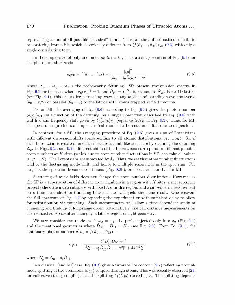
170 Publication: Probing Quantum Phases of Ultracold Atoms . . .
representing a sum of all possible “classical” terms. Thus, all these distributions contributeto scattering from a SF, which is obviously different from 〈f(n1, ..., nM )〉MI (9.3) with only asingle contributing term.
In the simple case of only one mode a0 (a1 ≡ 0), the stationary solution of Eq. (9.1) forthe photon number reads
a†0a0 = f(n1, ..., nM ) =|η0|2
(∆p − δ0D00)2 + κ2, (9.6)
where ∆p = ω0p − ω0 is the probe-cavity detuning. We present transmission spectra in
Fig. 9.2 for the case, where |u0(ri)|2 = 1, and D00 =∑K
i=1 ni reduces to NK . For a 1D lattice(see Fig. 9.1), this occurs for a traveling wave at any angle, and standing wave transverse(θ0 = π/2) or parallel (θ0 = 0) to the lattice with atoms trapped at field maxima.
For an MI, the averaging of Eq. (9.6) according to Eq. (9.3) gives the photon number
〈a†0a0〉MI, as a function of the detuning, as a single Lorentzian described by Eq. (9.6) withwidth κ and frequency shift given by δ0〈D00〉MI (equal to δ0NK in Fig. 9.2). Thus, for MI,the spectrum reproduces a simple classical result of a Lorentzian shifted due to dispersion.
In contrast, for a SF, the averaging procedure of Eq. (9.5) gives a sum of Lorentzianswith different dispersion shifts corresponding to all atomic distributions |q1, ..., qK〉. So, ifeach Lorentzian is resolved, one can measure a comb-like structure by scanning the detuning∆p. In Figs. 9.2a and 9.2c, different shifts of the Lorentzians correspond to different possibleatom numbers at K sites (which due to atom number fluctuations in SF, can take all values0,1,2,...,N). The Lorentzians are separated by δ0. Thus, we see that atom number fluctuationslead to the fluctuating mode shift, and hence to multiple resonances in the spectrum. Forlarger κ the spectrum becomes continuous (Fig. 9.2b), but broader than that for MI.
Scattering of weak fields does not change the atom number distribution. However, asthe SF is a superposition of different atom numbers in a region with K sites, a measurementprojects the state into a subspace with fixedNK in this region, and a subsequent measurementon a time scale short to tunneling between sites will yield the same result. One recoversthe full spectrum of Fig. 9.2 by repeating the experiment or with sufficient delay to allowfor redistribution via tunneling. Such measurements will allow a time dependent study oftunneling and buildup of long-range order. Alternatively, one can continue measurements onthe reduced subspace after changing a lattice region or light geometry.
We now consider two modes with ω0 = ω1, the probe injected only into a0 (Fig. 9.1)and the mentioned geometries where D00 = D11 = NK (see Fig. 9.3). From Eq. (9.1), the
stationary photon number a†1a1 = f(n1, ..., nM ) is
a†1a1 =δ21D
†10D10|η0|2
[∆′2p − δ21D†
10D10 − κ2]2 + 4κ2∆′2p
, (9.7)
where ∆′p = ∆p − δ1D11.
In a classical (and MI) case, Eq. (9.3) gives a two-satellite contour (9.7) reflecting normal-mode splitting of two oscillators 〈a0,1〉 coupled through atoms. This was recently observed [21]for collective strong coupling, i.e., the splitting δ1〈D10〉 exceeding κ. The splitting depends

171
Figure 9.2. Photon number in a single cavity mode. (a) Single Lorentzian for MI (curveA) reflects non-fluctuating atom number. Many Lorentzians for SF (curve B) reflect atomnumber fluctuations, which are imprinted on the positions of narrow resonances. Here κis smaller than satellite separation δ0 (κ = 0.1δ0), N = M = 30, K = 15. (b) The sameas in (a) but κ = δ0 gives smooth broadened contour for SF. (c) Spectra for SF withN = M = 70 and different number of sites illuminated K = 10, 35, 68. The transmissionspectra have different forms, since different atom distribution functions correspond todifferent K. κ = 0.05δ0.
on the geometry (see Eq. (9.1)) representing diffraction of one mode into another. Thus, ourresults can be treated as scattering from a “quantum diffraction grating” generalizing Braggscattering, well-known in different disciplines. In diffraction maxima (i.e. u∗
1(ri)u0(ri) = 1)one finds D10 = NK providing the maximal classical splitting. In diffraction minima, onefinds D10 =
∑Ki=1(−1)i+1ni providing both the classical splitting and photon number are
almost zero.
In SF, Eq. (9.5) shows that 〈a†1a1〉SF is given by a sum of all classical terms with all possiblenormal mode splittings. In a diffraction maximum (Figs. 9.3a,b), the right satellite is splitinto components corresponding to all possible NK or extremely broadened. In a minimum(Figs. 9.3c,d), the splittings are determined by all differences between atom numbers at oddand even sites
∑Ki=1(−1)i+1qi. Note that there is no classical description of the spectra in
a minimum, since here the classical field (and 〈a†1a1〉MI) are simply zero for any ∆p. Thus,for two cavities coupled at diffraction minimum, the difference between the SF and MI statesis even more striking: one has a structured spectrum instead of zero signal. Moreover, thedifference between atom numbers at odd and even sites fluctuates even for the whole latticeilluminated, giving nontrivial spectra even for K = M .

172 Publication: Probing Quantum Phases of Ultracold Atoms . . .
Figure 9.3. Photon number in one of two strongly coupled modes. (a) Diffractionmaximum, doublet for MI (curve A) and spectrum with structured right satellite for SF(curve B). Structure in the satellite reflects atom number fluctuations in SF, while narrowspectrum for MI demonstrates vanishing fluctuations. Here κ is smaller than satelliteseparation 2δ0 (κ = 0.1δ0), K = 15. (b) The same as in (a) but κ = δ0 gives broadenedsatellite for SF. (c) Diffraction minimum, zero field for MI and structured spectrum forSF. Nonzero structured spectrum for SF reflects fluctuating difference between atomnumbers at odd and even sites, which exists even for the whole lattice illuminated,K = M . Here κ is smaller than satellite separation 2δ0 (κ = 0.1δ0), K = 30. (d) Thesame as in (c) but κ = δ0 gives broadened contour for SF. N = M = 30 in all figures.
In each of the examples in Figs. 9.2 and 9.3, the photon number depends only on onestatistical quantity, now called q, f(q1, ..., qM ) = f(q). For the single mode and two modesin a maximum, q is the atom number at K sites. For two modes in a minimum, q is theatom number at odd (or even) sites. Therefore, expectation values for some state |Ψ〉 canbe reduced to 〈f〉Ψ =
∑Nq=0 f(q)pΨ(q), where pΨ(q) is the distribution function of q in this
state.
In high-Q cavities (κ δ0 = g2/∆0a), f(q) is given by a narrow Lorentzian of widthκ peaked at some frequency proportional to q (q = 0, 1, ..., N). The Lorentzian hight isq-independent. Thus, 〈f〉Ψ as a function of ∆p represents a comb of Lorentzians with theamplitudes simply proportional to pΨ(q).
This is our central result. It states that the transmission spectrum of a high-Q cavity〈a†a(∆p)〉Ψ directly maps the distribution function of ultracold atoms pΨ(q), e.g., distributionfunction of atom number at K sites. Various atomic statistical quantities characterizing aparticular state can be then calculated: mean value (given by the spectrum center), variance(determined by the spectral width) and higher moments. Furthermore, transitions between
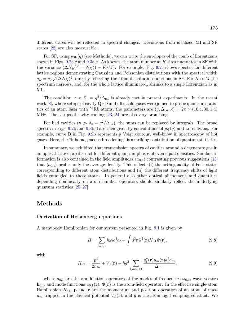
173
different states will be reflected in spectral changes. Deviations from idealized MI and SFstates [22] are also measurable.
For SF, using pSF(q) (see Methods), we can write the envelopes of the comb of Lorentziansshown in Figs. 9.2a,c and 9.3a,c. As known, the atom number at K sites fluctuates in SF withthe variance (∆NK)2 = NK(1 −K/M). For example, Fig. 9.2c shows spectra for differentlattice regions demonstrating Gaussian and Poissonian distributions with the spectral widthσω = δ0
√
(∆NK)2, directly reflecting the atom distribution functions in SF. For K ≈M thespectrum narrows, and, for the whole lattice illuminated, shrinks to a single Lorentzian as inMI.
The condition κ < δ0 = g2/∆0a is already met in present experiments. In the recentwork [8], where setups of cavity QED and ultracold gases were joined to probe quantum statis-tics of an atom laser with 87Rb atoms, the parameters are (g,∆0a, κ) = 2π × (10.4, 30, 1.4)MHz. The setups of cavity cooling [23, 24] are also very promising.
For bad cavities (κ δ0 = g2/∆0a), the sums can be replaced by integrals. The broadspectra in Figs. 9.2b and 9.3b,d are then given by convolutions of pΨ(q) and Lorentzians. Forexample, curve B in Fig. 9.2b represents a Voigt contour, well-know in spectroscopy of hotgases. Here, the “inhomogeneous broadening” is a striking contribution of quantum statistics.
In summary, we exhibited that transmission spectra of cavities around a degenerate gas inan optical lattice are distinct for different quantum phases of even equal densities. Similar in-formation is also contained in the field amplitudes 〈a0,1〉 contrasting previous suggestions [13]that 〈a0,1〉 probes only the average density. This reflects (i) the orthogonality of Fock statescorresponding to different atom distributions and (ii) the different frequency shifts of lightfields entangled to those states. In general also other optical phenomena and quantitiesdepending nonlinearly on atom number operators should similarly reflect the underlyingquantum statistics [25–27].
Methods
Derivation of Heisenberg equations
A manybody Hamiltonian for our system presented in Fig. 9.1 is given by
H =∑
l=0,1
~ωla†l al +
∫
d3rΨ†(r)Ha1Ψ(r), (9.8)
with
Ha1 =p2
2ma+ Vcl(r) + ~g2
∑
l,m=0,1
u∗l (r)um(r)a†l am∆ma
, (9.9)
where a0,1 are the annihilation operators of the modes of frequencies ω0,1, wave vectorsk0,1, and mode functions u0,1(r); Ψ(r) is the atom-field operator. In the effective single-atomHamiltonian Ha1, p and r are the momentum and position operators of an atom of massma trapped in the classical potential Vcl(r), and g is the atom–light coupling constant. We
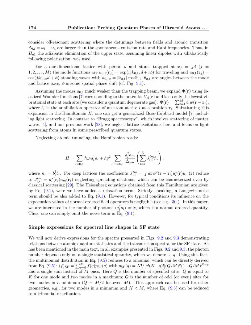
174 Publication: Probing Quantum Phases of Ultracold Atoms . . .
consider off-resonant scattering where the detunings between fields and atomic transition∆la = ωl − ωa are larger than the spontaneous emission rate and Rabi frequencies. Thus, inHa1 the adiabatic elimination of the upper state, assuming linear dipoles with adiabaticallyfollowing polarization, was used.
For a one-dimensional lattice with period d and atoms trapped at xj = jd (j =1, 2, . . . ,M) the mode functions are u0,1(rj) = exp(ijk0,1xd+ iφ) for traveling and u0,1(rj) =cos(jk0,1xd+ φ) standing waves with k0,1x = |k0,1| cos θ0,1, θ0,1 are angles between the modeand lattice axes, φ is some spatial phase shift (cf. Fig. 9.1).
Assuming the modes a0,1 much weaker than the trapping beam, we expand Ψ(r) using lo-calized Wannier functions [7] corresponding to the potential Vcl(r) and keep only the lowest vi-brational state at each site (we consider a quantum degenerate gas): Ψ(r) =
∑Mi=1 biw(r− ri),
where bi is the annihilation operator of an atom at site i at a position ri. Substituting thisexpansion in the Hamiltonian H, one can get a generalized Bose-Hubbard model [7] includ-ing light scattering. In contrast to “Bragg spectroscopy”, which involves scattering of matterwaves [4], and our previous work [28], we neglect lattice excitations here and focus on lightscattering from atoms in some prescribed quantum states.
Neglecting atomic tunneling, the Hamiltonian reads:
H =∑
l=0,1
~ωla†l al + ~g2
∑
l,m=0,1
a†l am∆ma
(
K∑
i=1
J lmi,i ni
)
,
where ni = b†ibi. For deep lattices the coefficients J lmi,i =∫
drw2(r − ri)u∗l (r)um(r) reduce
to J lmi,i = u∗l (ri)um(ri) neglecting spreading of atoms, which can be characterized even byclassical scattering [29]. The Heisenberg equations obtained from this Hamiltonian are givenby Eq. (9.1), were we have added a relaxation term. Strictly speaking, a Langevin noiseterm should be also added to Eq. (9.1). However, for typical conditions its influence on theexpectation values of normal ordered field operators is negligible (see e.g. [30]). In this paper,
we are interested in the number of photons 〈a†l al〉 only, which is a normal ordered quantity.Thus, one can simply omit the noise term in Eq. (9.1).
Simple expressions for spectral line shapes in SF state
We will now derive expressions for the spectra presented in Figs. 9.2 and 9.3 demonstratingrelations between atomic quantum statistics and the transmission spectra for the SF state. Ashas been mentioned in the main text, in all examples presented in Figs. 9.2 and 9.3, the photonnumber depends only on a single statistical quantity, which we denote as q. Using this fact,the multinomial distribution in Eq. (9.5) reduces to a binomial, which can be directly derivedfrom Eq. (9.5): 〈f〉SF =
∑Nq=0 f(q)pSF(q) with pSF(q) = N !/[q!(N−q)!](Q/M)q(1−Q/M)N−q
and a single sum instead of M ones. Here Q is the number of specified sites: Q is equal toK for one mode and two modes in a maximum; Q is the number of odd (or even) sites fortwo modes in a minimum (Q = M/2 for even M). This approach can be used for othergeometries, e.g., for two modes in a minimum and K < M , where Eq. (9.5) can be reducedto a trinomial distribution.

175
As a next approximation we consider N,M 1, but finite N/M , leading to the Gaussiandistribution pSF(q) = 1/(
√2πσq) exp [−(q − q)2/2σ2
q ] with central value q = NQ/M and
width σq =√
N(Q/M)(1 −Q/M).
In high-Q cavities (κ δ0 = g2/∆0a), f(q) is a narrow Lorentzian of width κ peakedat some q-dependent frequency, now called ∆q
p. Since the Lorentzian hight is q-independent,〈f〉SF as a function of ∆p is a comb of Lorentzians with the amplitudes proportional to pSF(q).
Using the Gaussian distribution pSF(q),we can write the envelope of such a comb. For asingle mode [Fig. 9.2a,c, Eq. (9.6)], we find ∆q
p ≈ δ0q with the envelope
〈a†0a0(∆qp)〉SF =
αδ0√2πσω
e−(∆qp−∆p)2/2σ2
ω ,
where the central frequency ∆p = δ0NK , spectral width σω = δ0√
NK(1−K/M), and α =|η0|2/κ2. So, the spectrum envelopes in Fig. 9.2a,c are well described by Gaussians of widthsstrongly depending on K.
For K → 0 and K → M , the binomial distribution pSF(q) is well approximated by aPoissonian distribution, which is demonstrated in Fig. 9.2c for K = 10 and K = 68. ForK = M the spectrum shrinks to a single Lorenzian, since the total atom number at M sitesdoes not fluctuate.
In other examples (Figs. 9.3a and 9.3c), the above expression is also valid, althoughwith other parameters. For two modes in a diffraction maximum (Fig. 9.3a), the centralfrequency, separation between Lorentzians and width are doubled: ∆p = 2δ0NK , ∆q
p ≈ 2δ0qand σω = 2δ0
√
NK(1−K/M); α = |η0|2/(2κ2). The left satellite at ∆p = 0 has a classicalamplitude |η0|2/(4κ2).
The nonclassical spectrum for two waves in a diffraction minimum (Fig. 9.3c) is centeredat ∆p = δ0N , with components at ∆q
p ≈ 2δ0q, and is very broad, σω = δ0√N ; α = |η0|2/κ2.
For bad cavities (κ δ0), the sums can be replaced by integrals with the same parameters∆p and σω as for κ < δ0. For a single mode, Fig. 9.2b represents a Voigt contour
〈a†0a0(∆p)〉SF =|η0|2√2πσω
∫ ∞
0
e−(ω−∆p)2/2σ2ωdω
(∆p − ω)2 + κ2.
For two modes in a diffraction minimum the photon number (Fig. 9.3d) is
〈a†1a1〉SF =|η0|2√2πσω
∫ ∞
−∞
ω2e−ω2/2σ2
ωdω
(∆′2p − ω2 − κ2)2 + 4κ2∆′2
p
,
where ∆′p = ∆p − ∆p, while in a maximum (Fig. 9.3b)
〈a†1a1〉SF =|η0|2
4√
2πσω
∫ ∞
0
ω2e−(ω−∆p)2/2σ2ωdω
[∆p(∆p − ω) + κ2]2 + κ2ω2.
176 Publication: Probing Quantum Phases of Ultracold Atoms . . .
Bibliography
[1] Bloch, I. Ultracold quantum gases in optical lattices. Nat. Phys. 1, 23–30 (2005).
[2] Folling, S. et al. Spatial quantum noise interferometry in expanding ultracold atomclouds. Nature 434, 481–484 (2005).
[3] Altman, E., Demler, E., & Lukin, M. D. Probing many-body states of ultracold atomsvia noise correlations. Phys. Rev. A 70, 013603 (2004).
[4] Stoferle, T., Moritz, H., Schori, C., Kohl, M. & Esslinger, T. Transition from a stronglyinteracting 1D superfluid to a Mott insulator. Phys. Rev. Lett. 92, 130403 (2004).
[5] Gritsev, V., Altman, E., Demler, E. & Polkovnikov, A. Full quantum distribution ofcontrast in interference experiments between interacting one-dimensional Bose liquids.Nat. Phys. 2, 705–709 (2006).
[6] Schellekens, M. et al. Hanbury Brown Twiss effect for ultracold quantum gases. Science310, 648–651 (2005).
[7] Jaksch, D., Bruder, C., Cirac, J. I., Gardiner, C. W. & Zoller, P. Cold bosonic atoms inoptical lattices Phys. Rev. Lett. 81, 3108–3111 (1998).
[8] Bourdel, T. et al. Cavity QED detection of interfering matter waves. Phys. Rev. A 73,043602 (2006).
[9] You, L., Lewenstein, M. & Cooper, J. Line shapes for light scattered from Bose-Einsteincondensates. Phys. Rev. A 50, R3565–R3568 (1994).
[10] Javanainen, J. Optical signatures of a tightly confined Bose condensate. Phys. Rev. Lett.72, 2375–2378 (1994).
[11] You, L., Lewenstein, M., & Cooper, J. Quantum field theory of atoms interacting withphotons. II. Scattering of short laser pulses from trapped bosonic atoms. Phys. Rev. A51, 4712–4727 (1995).
[12] Javanainen, J. & Ruostekoski, J. Off-resonance light scattering from low-temperatureBose and Fermi gases. Phys. Rev. A 52, 3033–3046 (1995).
[13] Parkins, A. S. & Walls, D. F. The physics of trapped dilute-gas Bose-Einstein conden-sates. Phys. Rep. 303, 1-80 (1998).
[14] Morice, O., Castin, Y. & Dalibard, J. Refractive index of a dilute Bose gas. Phys. Rev.A 51, 3896–3901 (1995).
[15] Brune, M., et al. Quantum Rabi oscillation: a direct test of field quantization in a cavity.Phys. Rev. Lett. 76, 1800–1803 (1996).
[16] Gambetta, J. et al. Qubit-photon interactions in a cavity: Measurement-induced de-phasing and number splitting. Phys. Rev. A 74, 042318 (2006).
BIBLIOGRAPHY 177
[17] Campbell, G. K. et al. Imaging the Mott insulator shells by using atomic clock shifts.Science 313, 649–652 (2006).
[18] Gerbier, F., Folling, S., Widera, A., Mandel, O. & Bloch, I. Probing number squeezingof ultracold atoms across the superfluid-Mott insulator transition. Phys. Rev. Lett. 96,090401 (2006).
[19] Volz, T. et al. Preparation of a quantum state with one molecule at each site of an opticallattice. Nat. Phys. 2, 692–695 (2006).
[20] Winkler, K. et al. Repulsively bound atom pairs in an optical lattice. Nature 441, 853–856 (2006).
[21] Klinner, J., Lindholdt, M., Nagorny, B. & Hemmerich, A. Normal mode splitting andmechanical effects of an optical lattice in a ring cavity. Phys. Rev. Lett. 96, 023002(2006).
[22] Lewenstein, M. et al. Ultracold atomic gases in optical lattices: Mimicking condensedmatter physics and beyond. cond-mat/0606771.
[23] Maunz, P. et al. Cavity cooling of a single atom. Nature 428, 50–52 (2004).
[24] Hood, C. J., Lynn, T. W., Doherty, A. C., Parkins, A. S. & Kimble, H. J. The atom-cavity microscope: single atoms bound in orbit by single photons. Science 287, 1447–1453 (2000).
[25] Mekhov, I. B., Maschler, C. & Ritsch, H. Cavity enhanced light scattering in opticallattices to probe atomic quantum satistics. quant-ph/0610073.
[26] Mekhov, I. B., Maschler, C. & Ritsch, H., Light scattering from atoms in an opticallattice: optical probe of quantum statisticsin, Books of abstracts for the XX InternationalConference on Atomic Physics, ICAP, Innsbruck, 2006, p. 309 and conference web-site.
[27] Chen, W., Meiser, D. & Meystre, P. Cavity QED determination of atomic numberstatistics in optical lattices. quant-ph/0610029.
[28] Maschler, C. & Ritsch, H. Cold atom dynamics in a quantum optical lattice potential.Phys. Rev. Lett. 95, 260401 (2005).
[29] Slama, S., von Cube, C., Kohler, M., Zimmermann, C. & Courteille, P. V. Multiplereflections and diffuse scattering in Bragg scattering at optical lattices. Phys. Rev. A 73,023424 (2006).
[30] Davidovich, L. Sub-Poissonian processes in quantum optics. Rev. Mod. Phys. 68, 127(1996).
178 Publication: Probing Quantum Phases of Ultracold Atoms . . .
Acknowledgments
The work was supported by FWF (P17709 and S1512). While preparing this manuscript, webecame aware of a closely related research in the group of P. Meystre. We are grateful tohim for sending us the preprint [27] and stimulating discussions.
Correspondence and request for materials should be addressed to I.B.M.
Competing financial interests
The authors declare that they have no competing financial interests.
Part III
Self-Organization of Atoms inOptical Lattices


Chapter 10
Background: Self-Organization of Atoms in a
Cavity
The last part of this thesis is devoted to a microscopic view on the self-organizationprocess of atoms in a cavity field and its onset. In this background chapter we present aqualitative overview of the phenomenon of self-organizing atoms into a regular lattice in acavity field, first investigated in our group [1]. In our studies here, we consider motion of theatoms along the direction of the pumping laser. This leads to slightly simplified calculations,but essentially contains all the underlying physics. The single-particle Hamiltonian for thissituation, was derived in Sec. 3.3. Since this self-organization process, of course, relies onmany-body physics, we have to derive a corresponding Bose-Hubbard Hamiltonian, as well.This can be found in the second part of this chapter.
Some of the results in the subsequent chapters have been obtained with Monte-Carlo wavefunction simulations, performed by Andras Vukics. In order to avoid an overloading of thisthesis, we will not present a background chapter on the Monte-Carlo method, and insteadrefer to [2].
10.1 Collective Cooling and Spatial Self-Organization of
Atoms
The strong coupling of a single atom inside a high-Q optical resonator allows for efficientcooling and trapping of this atom [3–7]. The underlying cooling mechanism is fundamen-tally different to usual laser cooling schemes and relies on the complex nonlinear interactionbetween cavity field and atom and on the presence of a dissipation channel, independent ofspontaneous emission. Essentially, the atom scatters into the cavity mode, which can losephotons and hence energy via the cavity mirrors.
Conventional laser cooling schemes are not altered by the presence of many atoms, sincethey depend merely on single atom processes. For resonator-induced forces, though, this isdrastically different. Here, all atoms interact, mediated by the intracavity field, to which allatoms are simultaneously coupled. Hence, the positions and velocities of the atoms influenceeach other and modify the scattering properties of each atom and therewith the coolingprocess. This leads to cooperative effects, providing for perspectives to significantly enhancethe cooling efficiency.
This cooperative effect requires direct coherent driving of the atoms instead of excitingthe cavity mode. We presented this so-called “atom pumping” setup already in chapters 5and 6. We consider N two-level atoms, transversally illuminated by a red-detuned pumpinglaser (see Fig. 10.1). The atoms scatter photons in the cavity mode, with a field amplitude
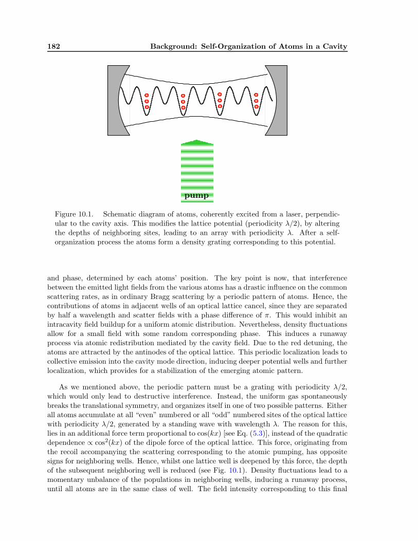
182 Background: Self-Organization of Atoms in a Cavity
Figure 10.1. Schematic diagram of atoms, coherently excited from a laser, perpendic-ular to the cavity axis. This modifies the lattice potential (periodicity λ/2), by alteringthe depths of neighboring sites, leading to an array with periodicity λ. After a self-organization process the atoms form a density grating corresponding to this potential.
and phase, determined by each atoms’ position. The key point is now, that interferencebetween the emitted light fields from the various atoms has a drastic influence on the commonscattering rates, as in ordinary Bragg scattering by a periodic pattern of atoms. Hence, thecontributions of atoms in adjacent wells of an optical lattice cancel, since they are separatedby half a wavelength and scatter fields with a phase difference of π. This would inhibit anintracavity field buildup for a uniform atomic distribution. Nevertheless, density fluctuationsallow for a small field with some random corresponding phase. This induces a runawayprocess via atomic redistribution mediated by the cavity field. Due to the red detuning, theatoms are attracted by the antinodes of the optical lattice. This periodic localization leads tocollective emission into the cavity mode direction, inducing deeper potential wells and furtherlocalization, which provides for a stabilization of the emerging atomic pattern.
As we mentioned above, the periodic pattern must be a grating with periodicity λ/2,which would only lead to destructive interference. Instead, the uniform gas spontaneouslybreaks the translational symmetry, and organizes itself in one of two possible patterns. Eitherall atoms accumulate at all “even” numbered or all “odd” numbered sites of the optical latticewith periodicity λ/2, generated by a standing wave with wavelength λ. The reason for this,lies in an additional force term proportional to cos(kx) [see Eq. (5.3)], instead of the quadraticdependence ∝ cos2(kx) of the dipole force of the optical lattice. This force, originating fromthe recoil accompanying the scattering corresponding to the atomic pumping, has oppositesigns for neighboring wells. Hence, whilst one lattice well is deepened by this force, the depthof the subsequent neighboring well is reduced (see Fig. 10.1). Density fluctuations lead to amomentary unbalance of the populations in neighboring wells, inducing a runaway process,until all atoms are in the same class of well. The field intensity corresponding to this final

10.1. Collective Cooling and Spatial Self-Organization of Atoms 183
state depends quadratically on the atom number N , an obvious sign of the cooperativity inthis process. For a suitable choice of parameters, this process leads to efficient cooling andtrapping of the atoms, by means of the cavity loss, which dissipates the increased kineticenergy of the atoms, when they fall into the lattice wells. Heating processes limit the coolingtemperature to some finite value.
In seminal experiments by Vuletic and coworkers [8–10], strongly enhanced emission (byorders of magnitude) was observed, as soon as the pumping laser intensity exceeded a cer-tain threshold. This led to efficient cooling of large ensembles. Since a phase difference ofπ between the two possible regular gratings exist, a heterodyne measurement of the timephase allows to observe the symmetry breaking between the two patterns, induced by densityfluctuations.
Moreover, this self-organization effect persists also in a two-dimensional situation, if thepumping field is a standing wave field, generated by counterpropagating laser beams. Here,the atoms organize in one of two equivalent rectangular arrays in form of a checkerboard. InFig. 10.2, we schematically depict the two patterns and their spatial offset, leading to thephase difference in the scattered light.
Figure 10.2. In two dimensions the atoms self-organize in a checkerboard pattern. Thetwo different but equivalent density gratings, depicted by blue and red balls, emit lightinto the cavity mode with a phase difference of π.
An additional point has to be added to the above discussion. Zippilli et al. [11, 12]argued that, if the pumping field is close to resonance, Bragg scattering cannot explain thedramatic suppression of atomic fluorescence, which allows the cavity loss to be the dominantdissipation channel. In fact, for atom numbers below a certain threshold value, i.e. N N0,the intensity of the cavity field depends quadratically on the atom number, and the numberof excited atoms is close to the free-space excitation population. The resulting enhancementof the scattering rate into the cavity can be well described by Bragg scattering. However, for
184 Background: Self-Organization of Atoms in a Cavity
N N0, the total power of dissipation via spontaneous emission loses ground, since it scalesas 1/N . In this regime, leaking of cavity photons is the main dissipation channel and theintracavity intensity is approximately constant and independent of N . A closer look reveals,that for ∆c ≈ 0 and κ < Γ, the cavity field and the pumping laser field have opposite phasesand mutually cancel at atomic positions. Hence, the atoms localize at positions, where atomicexcitations and fluorescence are strongly suppressed. Therefore, the ratio of scattering in thecavity mode to free-space scattering increases with N , even in the saturation regime, wherethe intensity of the cavity field is constant.
Note, that this collective effect is different to other, recently demonstrated, collective phe-nomena. For the collective atomic recoil laser in a ring cavity (CARL) [13–17], a magneto-optical trap is required, in order to stabilize the atoms, since their center of mass is continu-ously accelerated by the CARL process.
10.2 The Bose-Hubbard Hamiltonian for Transverse Motion
In Sec. 3.3 we described the setup for our studies concerning the onset of the self-organizationprocess, to which this chapter is devoted. We considered motion of particles, in the opticallattice, generated by the pumping laser field. The coupling of the particles to the cavitymode, though, is responsible for collective effects, including the self-ordering of particles inone of two stable patterns.
In this section we have to correctly address a single particle Hamiltonian, which we im-plement in a second-quantized Hamiltonian, allowing for a many-body description. Startingfrom (3.51), we adiabatically eliminate the excited states simply by replacing the Pauli ma-trices σ± by their steady state values
σ− = −ζ cos(kpy) + g0 cos(kx)a
γ − i∆aand σ+ = −ζ cos(kpy) + g0 cos(kx)a†
γ + i∆a. (10.1)
Here kp denotes the wavenumber of the pumping field lattice, whereas k is the wavenumber ofthe cavity lattice. To the contrary of (3.52), we incorporated the position in the cavity fieldvia cos(kx), which in fact is necessary in the second-quantized formalism. Nevertheless, sincewe neglect motion along the cavity axis, we can omit the momentum operator px and replacex by a c-number x0. Then, the replacement of the expressions for the excitation operatorsyield
Heff =p2y
2m− ~
[
∆c − U0 cos2(kx0)]
a†a+ V0 cos2(kpy)
+ sgn(U0)√
~U0V0 cos(kpy) cos(kx0)(
a+ a†)
, (10.2)
where the potential depth of the lattice corresponding to the pumping laser field and the cavityfield (per photon), respectively, are given by V0 = ~ζ2∆a/(γ
2+∆2a) and U0 = g2
0∆a/(γ2+∆2
a).The particle motion is now only one-dimensional, and we can apply the general second-quantized Hamiltonian (2.20). Here, we have to implement all terms, corresponding to par-ticle motion. Since cos2(kx0)a
†a originally depended on particle motion, we will include also

10.2. The Bose-Hubbard Hamiltonian for Transverse Motion 185
this term. Furthermore, without loss of generality, we can set x0 = 0. Hence, we get:
H =
∫
R
dy؆(y)
[
p2y
2m+ V0 cos2(kpy) + sgn(U0)
√
~U0V0 cos(kpy)(
a+ a†)
+ ~U0a†a
]
Ψ(y)
− ~∆ca†a+
1
2
∫
R
∫
R
dxdyΨ†(x)Ψ†(y)U(x, y)Ψ(x)Ψ(y). (10.3)
Here Ψ(y) denotes the field operator for the bosonic particles. Now, proceeding along thelines of Sec. 2.3.1, we consider one-dimensional on-site interactions U(x, y) = g1Dδ(x−y) andexpand the field operator in the Wannier basis, where we only take the lowest energy bandinto account, i.e.
Ψ(x) =M∑
i=1
w(x− xi)bi. (10.4)
Here w(x) is the Wannier function, corresponding to the lowest band, and bi is the bosonicannihilation operator for a particle at site i. Moreover, the same arguments concerning therelevance of the various tunneling contributions as in Sec. 2.3.1 are valid. Hence, we onlyhave to consider next-neighbor hopping and only one term for the on-site interactions. Here,due to the existence of cos(kpy), a new term appears, which allows the system to break thetranslational symmetry of the lattice. The associated matrix elements
Jkl = sgn(U0)√
~U0V0
∫
R
dy w(y − yk) cos(kpy)w(y − yl) (10.5)
have vanishing values for tunneling, i.e. Jn,n±1 = 0 for all n, if we neglect tunneling to otherthen adjacent sites:
Jn,n±1
sgn(U0)√
~U0V0=
∫
R
dy w(y − yn±1) cos(kpy)w(y − yn)
= (−1)n∫
R
dy w(y ± a) cos(kpy)w(y)
= ±(−1)n∫
R
dy w(
y +a
2
)
sin(kpy)w(
y − a
2
)
= 0,
since w(y + a/2)w(y − a/2) is even (a = π/k). A similar argument shows, that the on-siteelements have alternating signs, i.e. Jn,n = −Jn±1,n±1. As a last step, the assumption of aconstant atom number, allows to neglect constant terms in the second quantized Hamiltonian:
H = J∑
〈k,l〉b†kbl + J
∑
k
(−1)knk
(
a+ a†)
− (∆c −NU0)a†a+
U
2
∑
k
nk(nk − 1). (10.6)
Note, that to the contrary of chapter 2, here J is the matrix element, corresponding to the
total energy J =∫
Rdy w(y − a)
(
− ~2
2md2
dy2+ V0 cos2(ky)
)
w(y). The operator for the particle
number at site k is denoted by nk = b†kbk and J = J00. This is the modified Bose-HubbardHamiltonian, providing for the many-body plus cavity field dynamics, which we use in theremaining two chapters of this thesis.1
1In chapter 12, the lattice definition is slightly different. There, the lattice potential is proportional tosin2(kpy), leading to lattice sites at yn = π/2 + na for n ∈ Z. Nevertheless, this amounts just to a globalphase shift, having no influence on matrix elements or any other properties of the dynamics.
186 Background: Self-Organization of Atoms in a Cavity
Bibliography
[1] P. Domokos and H. Ritsch, Collective Cooling and Self-Organization of Atoms in aCavity, Phys. Rev. Lett. 89, 253003 (2002).
[2] A. Vukics and H. Ritsch, C++QED: An Object-Oriented Framework for Wave-FunctionSimulations of Cavity QED Systems, Eur. J. Phys. D 44, 585 (2007).
[3] P. Horak, G. Hechenblaikner, K. M. Gheri, H. Stecher, and H. Ritsch, Cavity-InducedAtom Cooling in the Strong Coupling Regime, Phys. Rev. Lett. 79, 4974 (1997).
[4] G. Hechenblaikner, M. Gangl, P. Horak, and H. Ritsch, Cooling an Atom in a WeaklyDriven High-Q Cavity, Phys. Rev. A 58, 3030 (1998).
[5] C. J. Hood, T. W. Lynn, A. C. Doherty, A. S. Parkins, and H. J. Kimble, The Atom-Cavity Microscope: Single Atoms Bound in Orbit by Single Photons, Science 287, 1447(2000).
[6] P. W. H. Pinkse, T. Fischer, P. Maunz, and G. Rempe, Trapping an Atom with SinglePhotons, Nature (London) 404, 365 (2000).
[7] P. Maunz, T. Puppe, I. Schuster, N. Syassen, P. W. H. Pinkse, and G. Rempe, CavityCooling of a Single Atom, Nature (London) 428, 50 (2004).
[8] H. W. Chan, A. T. Black, and V. Vuletic, Observation of Collective-Emission-InducedCooling of Atoms in an Optical Cavity, Phys. Rev. Lett. 90, 063003 (2003).
[9] A. T. Black, H. W. Chan, and V. Vuletic, Observation of Collective Friction Forces Dueto Spatial Self-Organization of Atoms: From Rayleigh to Bragg Scattering, Phys. Rev.Lett. 91, 203001 (2003).
[10] A. T. Black, J. K. Thompson, and V. Vuletic, Collective Light Forces on Atoms inResonators, J. Phys. B: At. Mol. Opt. Phys. 38, 605 (2005).
[11] S. Zippilli, G. Morigi, and H. Ritsch, Suppression of Bragg Scattering by CollectiveInterference of Spatially Ordered Atoms with a High-Q Cavity Mode, Phys. Rev. Lett.93, 123002 (2004).
[12] S. Zippilli, G. Morigi, and H. Ritsch, Collective Effects in the Dynamics of Driven Atomsin a High-Q Cavity, Eur. Phys. J. D 31, 507 (2004).
[13] D. Kruse, C. von Cube, C. Zimmermann, and Ph. W. Courteille, Observation of LasingMediated by Collective Atomic Recoil, Phys. Rev. Lett. 91, 183601 (2003).
[14] B. Nagorny, Th. Elsasser, and A. Hemmerich, Collective Atomic Motion in an OpticalLattice Formed Inside a High-Finesse Cavity, Phys. Rev. Lett. 91, 153003 (2003).
[15] Th. Elsasser, B. Nagorny, and A. Hemmerich, Optical Bistability and Collective Behaviorof Atoms Trapped in a High-Q Ring Cavity, Phys. Rev. A 69, 033403 (2004).
BIBLIOGRAPHY 187
[16] C. von Cube, S. Slama, D. Kruse, C. Zimmermann, Ph. W. Courteille, G. R. M. Robb,N. Piovella, and R. Bonifacio, Self-Synchronization and Dissipation-Induced Thresholdin Collective Atomic Recoil Lasing, Phys. Rev. Lett. 93, 083601 (2004).
[17] S. Slama, C. von Cube, B. Deh, A. Ludewig, C. Zimmermann, Ph. W. Courteille, Phase-Sensitive Detection of Bragg Scattering at 1D Optical Lattices, Phys. Rev. Lett. 94,193901 (2005).

Chapter 11
Publication
Entanglement Assisted Fast Reordering of Atoms in an
Optical Lattice within a Cavity at T = 0†
Optics Communications 273, 446 (2007)
C. Maschler1, H. Ritsch1, A. Vukics2, and P. Domokos2
1) Institut fur theoretische Physik, Universitat Innsbruck,A-6020 Innsbruck, Austria
2) Research Institute of Solid State Physics and Optics, Hungarian Academy of Sciences,H-1525 Budapest P.O. Box 49, Hungary
Laser-illuminated atoms in an optical resonator exhibit a phase transition betweenthe homogenous distribution and two possible ordered configurations in the optical latticeformed by the cavity and pump fields. At zero temperature, atom-field entanglementplays a crucial role in the spatial reordering of the atoms from a homogeneous towardsthe two ordered states, where all atoms occupy either only even or only odd latticesites. Concurrent with the buildup of atom-field entanglement, the homogeneous atomiccloud evolves immediately into the superposition of the two stable patterns entangledwith opposite cavity field amplitudes. This possibility is absent in a factorized (classical)treatment of atoms and field and should be generic for spontaneous symmetry breakingin quantum phase transitions in optical potentials.
Laser light with spatially modulated intensity, far red detuned from an atomic resonancecreates a designable optical potential to trap and manipulate ultra-cold atoms [1]. Con-structing a periodic lattice potential enables tailored implementations of the Bose-HubbardHamiltonian [2] to study quantum phase transitions [3] or ideas of quantum informationprocessing [4]. Whilst the effect of a free-space laser field can be well approximated by anexternal potential via factorizing field and atomic dynamics, a field enclosed in a cavity isinfluenced by the atoms and takes part in the coupled atom-field dynamics [5, 10]. Nowadaysin optical cavity QED using cold atoms in high finesse Fabry-Perot resonators the regime ofstrong light-matter interaction is experimentally accessible [6–8]. Here even a single cavityphoton exerts significant forces and the quantum properties of the optical forces can no longerbe ignored [9, 11].
†The primary contribution of the author of the present thesis to this publication were the calculationsconcerning the Bose-Hubbard model, while the Monte Carlo calculations were performed by A. V. The toymodel was described by H. R. The author of the present thesis also acted as a discussion partner for all theaspects of this work.
190 Publication: Entanglement Assisted Fast Reordering of Atoms . . .
In this paper we discuss some fundamental consequences of the back-action of a particle’smotion on the potential it moves in. In particular, we concentrate on the physics of suchan intrinsic feedback mechanism at the quantum level. Here the potential and thus theforce the particles feel can be in a superposition state entangled with their position. As anexperimentally accessible example we consider a laser-illuminated degenerate gas moving inthe optical potential generated by a high-Q cavity field. As theoretically predicted [12] andsubsequently demonstrated in experiment [13] this system exhibits a phase transition in theclassical, thermal gas limit [14].
This phenomenon is briefly summarized as follows. For red detuning (high field seekingatoms), above a threshold pump intensity the atoms spontaneously break the continuoustranslational symmetry along the cavity axis (see the geometry in Fig. 11.1(b), although inthis paper the motion will be restricted only along the pump field) and form one of tworegular patterns that maximize light scattering from the pump into the cavity. Here theatoms arrange along Bragg planes optimally coupling the pump and the cavity fields. Thetwo possible patterns (their configuration is similar to the black and white fields of a checker-board) lead to superradiant light scattering proportional to the square of the particle number,however, with opposite phases of the cavity field amplitude. For a thermal cloud, the onsetof self- organization can be understood as originating from an amplification of the atomicdensity fluctuations by feedback through the cavity field. For a random distribution of atomson different lattice sites the scattering into the cavity mode enlarges the potential depth ofthose lattice sites, where more atoms sit. This subsequently leads to trapping of more atomsat these sites in a runaway process towards the ordered pattern.
In this paper we will concentrate on the regime of quantized atomic motion at T =0, where the onset of atomic order and symmetry breaking is more intricate. Using anatomic BEC as an initial state the atoms have a kinetic energy much less than the recoilenergy so that their wave function is flat on the wavelength scale [8]. Since the atomsform a linear refractive medium in the large atom-field detuning limit and coherent high-intensity pumping is employed, it is tempting to use a “classical” (mean-field) descriptionof the scattered light field and calculate the back-action using a mean-field approximationof the condensate. This approximate mean-field model predicts that no light is scatteredinto the cavity from the initially homogeneous atomic distribution as the field amplitudesscattered into the cavity from different parts of the atomic wave function separated by halfa wavelength interfere destructively. Thus one expects no light scattering at start and self-organization would occur on a very slow time scale only due to an eventual asymmetry ofthe initial wavefunction. As we will show later in this work, this conclusion is only valid fora “classical” (or factorized) description of the cavity field amplitude as it it is widely appliedfor off resonant light scattering [15].
The cavity field in fact realizes a quantum feedback [16] for the atomic motion in whichatom-field entanglement is a crucial element. In this case scattered field amplitudes with op-posite phases do not necessarily cancel, but entangle to different atomic wave functions [17].If these are orthogonal, “which way information” prevents the interference of the correspond-ing field amplitudes. Although the quantum average of the field amplitude is zero, the photonnumber in the cavity can grow fast. This is clearly incompatible with a classical field ap-proximation or a factorization of the atom and field dynamics. The important point nowis that the two opposite phase components of the cavity field superposition create opposite
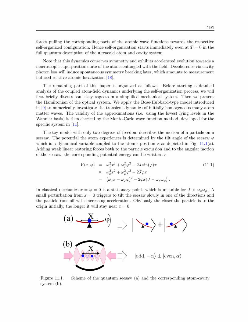
191
forces pulling the corresponding parts of the atomic wave functions towards the respectiveself-organized configuration. Hence self-organization starts immediately even at T = 0 in thefull quantum description of the ultracold atom and cavity system.
Note that this dynamics conserves symmetry and exhibits accelerated evolution towards amacroscopic superposition state of the atoms entangled with the field. Decoherence via cavityphoton loss will induce spontaneous symmetry breaking later, which amounts to measurementinduced relative atomic localization [18].
The remaining part of this paper is organized as follows. Before starting a detailedanalysis of the coupled atom-field dynamics underlying the self-organization process, we willfirst briefly discuss some key aspects in a simplified mechanical system. Then we presentthe Hamiltonian of the optical system. We apply the Bose-Hubbard-type model introducedin [9] to numerically investigate the transient dynamics of initially homogeneous many-atommatter waves. The validity of the approximations (i.e. using the lowest lying levels in theWannier basis) is then checked by the Monte-Carlo wave function method, developed for thespecific system in [11].
The toy model with only two degrees of freedom describes the motion of a particle on aseesaw. The potential the atom experiences is determined by the tilt angle of the seesaw ϕwhich is a dynamical variable coupled to the atom’s position x as depicted in Fig. 11.1(a).Adding weak linear restoring forces both to the particle excursion and to the angular motionof the seesaw, the corresponding potential energy can be written as
V (x, ϕ) = ω2xx
2 + ω2ϕϕ
2 − 2J sin(ϕ)x (11.1)
≈ ω2xx
2 + ω2ϕϕ
2 − 2Jϕx
= (ωxx− ωϕϕ)2 − 2ϕx(J − ωxωϕ) .
In classical mechanics x = ϕ = 0 is a stationary point, which is unstable for J > ωxωϕ. Asmall perturbation from x = 0 triggers to tilt the seesaw slowly in one of the directions andthe particle runs off with increasing acceleration. Obviously the closer the particle is to theorigin initially, the longer it will stay near x = 0.
Figure 11.1. Scheme of the quantum seesaw (a) and the corresponding atom-cavitysystem (b).
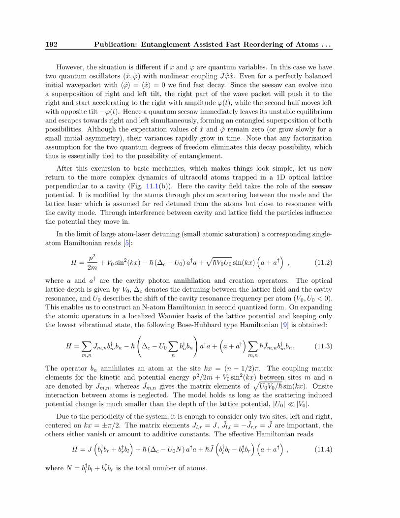
192 Publication: Entanglement Assisted Fast Reordering of Atoms . . .
However, the situation is different if x and ϕ are quantum variables. In this case we havetwo quantum oscillators (x, ϕ) with nonlinear coupling Jϕx. Even for a perfectly balancedinitial wavepacket with 〈ϕ〉 = 〈x〉 = 0 we find fast decay. Since the seesaw can evolve intoa superposition of right and left tilt, the right part of the wave packet will push it to theright and start accelerating to the right with amplitude ϕ(t), while the second half moves leftwith opposite tilt −ϕ(t). Hence a quantum seesaw immediately leaves its unstable equilibriumand escapes towards right and left simultaneously, forming an entangled superposition of bothpossibilities. Although the expectation values of x and ϕ remain zero (or grow slowly for asmall initial asymmetry), their variances rapidly grow in time. Note that any factorizationassumption for the two quantum degrees of freedom eliminates this decay possibility, whichthus is essentially tied to the possibility of entanglement.
After this excursion to basic mechanics, which makes things look simple, let us nowreturn to the more complex dynamics of ultracold atoms trapped in a 1D optical latticeperpendicular to a cavity (Fig. 11.1(b)). Here the cavity field takes the role of the seesawpotential. It is modified by the atoms through photon scattering between the mode and thelattice laser which is assumed far red detuned from the atoms but close to resonance withthe cavity mode. Through interference between cavity and lattice field the particles influencethe potential they move in.
In the limit of large atom-laser detuning (small atomic saturation) a corresponding single-atom Hamiltonian reads [5]:
H =p2
2m+ V0 sin2(kx)− ~ (∆c − U0) a
†a+√
~V0U0 sin(kx)(
a+ a†)
, (11.2)
where a and a† are the cavity photon annihilation and creation operators. The opticallattice depth is given by V0, ∆c denotes the detuning between the lattice field and the cavityresonance, and U0 describes the shift of the cavity resonance frequency per atom (V0, U0 < 0).This enables us to construct an N-atom Hamiltonian in second quantized form. On expandingthe atomic operators in a localized Wannier basis of the lattice potential and keeping onlythe lowest vibrational state, the following Bose-Hubbard type Hamiltonian [9] is obtained:
H =∑
m,n
Jm,nb†mbn − ~
(
∆c − U0
∑
n
b†nbn
)
a†a+(
a+ a†)
∑
m,n
~Jm,nb†mbn. (11.3)
The operator bn annihilates an atom at the site kx = (n − 1/2)π. The coupling matrixelements for the kinetic and potential energy p2/2m + V0 sin2(kx) between sites m and nare denoted by Jm,n, whereas Jm,n gives the matrix elements of
√
U0V0/~ sin(kx). Onsiteinteraction between atoms is neglected. The model holds as long as the scattering inducedpotential change is much smaller than the depth of the lattice potential, |U0| |V0|.
Due to the periodicity of the system, it is enough to consider only two sites, left and right,centered on kx = ±π/2. The matrix elements Jl,r = J , Jl,l = −Jr,r = J are important, theothers either vanish or amount to additive constants. The effective Hamiltonian reads
H = J(
b†l br + b†rbl)
+ ~ (∆c − U0N) a†a+ ~J(
b†l bl − b†rbr)(
a+ a†)
, (11.4)
where N = b†l bl + b†rbr is the total number of atoms.
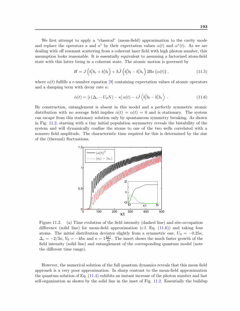
193
We first attempt to apply a “classical” (mean-field) approximation to the cavity modeand replace the operators a and a† by their expectation values α(t) and α∗(t). As we aredealing with off resonant scattering from a coherent laser field with high photon number, thisassumption looks reasonable. It is essentially equivalent to assuming a factorized atom-fieldstate with this latter being in a coherent state. The atomic motion is governed by
H = J(
b†l br + b†rbl)
+ ~J(
b†l bl − b†rbr)
2Re α(t) , (11.5)
where α(t) fulfills a c-number equation [9] containing expectation values of atomic operatorsand a damping term with decay rate κ:
α(t) = [i (∆c − U0N)− κ]α(t)− iJ⟨
b†l bl − b†rbr⟩
. (11.6)
By construction, entanglement is absent in this model and a perfectly symmetric atomicdistribution with no average field implies α(t) = α(t) = 0 and is stationary. The systemcan escape from this stationary solution only by spontaneous symmetry breaking. As shownin Fig. 11.2, starting with a tiny initial population asymmetry reveals the bistability of thesystem and will dynamically confine the atoms to one of the two wells correlated with anonzero field amplitude. The characteristic time required for this is determined by the sizeof the (thermal) fluctuations.
Figure 11.2. (a) Time evolution of the field intensity (dashed line) and site-occupationdifference (solid line) for mean-field approximation (c.f. Eq. (11.6)) and taking fouratoms. The initial distribution deviates slightly from a symmetric one, U0 = −0.25κ,∆c = −2/3κ, V0 = −4~κ and κ = 1~k2
m . The insert shows the much faster growth of thefield intensity (solid line) and entanglement of the corresponding quantum model (notethe different time range).
However, the numerical solution of the full quantum dynamics reveals that this mean fieldapproach is a very poor approximation. In sharp contrast to the mean-field approximationthe quantum solution of Eq. (11.4) exhibits an instant increase of the photon number and fastself-organization as shown by the solid line in the inset of Fig. 11.2. Essentially the buildup

194 Publication: Entanglement Assisted Fast Reordering of Atoms . . .
of a nonclassical field with atom-field entanglement in the quantum solution generates thisfast dynamics.
As a better approximation to the full quantum solution of Eq. (11.4) we formally solvethe operator Heisenberg equation for a in the bad cavity limit, where the field adiabaticallyfollows the atomic dynamics. The genuine quantum properties of the cavity field a are thenrepresented in terms of the atomic population difference operator:
a = −i J
κ− i(∆c − U0N)
(
b†l bl − b†rbr)
. (11.7)
As the atom number N = N is a constant of motion, the dynamics takes place in ir-reducible subspaces. It is instructive to consider first the single atom subspace where theentanglement-assisted decay, analogous to the quantum seesaw mechanism, can already beseized. For a single atom, b†i bi acts as a projector on the i-th well. Hence, depending onthe atom’s position the field 〈a〉 changes sign and vanishes for a symmetric atomic state.
However, the photon number operator a†a ∝(
b†l bl − b†rbr
)2is proportional to the unit oper-
ator in the single atom subspace, so that the photon number is nonzero independent of theatomic state and in particular also for a symmetric state. This implies that, in contrast tothe mean-field description, even a perfect symmetric initial population triggers the growth ofthe photon number although the mean field vanishes, 〈a〉 = 0.
Figure 11.3. Entanglement (solid lines), photon number (dot- dashed lines), and thetwo-site atom-atom correlation function (dotted lines) for two atoms in two wells. Lineswith extra circles show the case of exactly one atom in each well at start (Mott state),while the others correspond to a symmetric superposition state for each atom (superfluidstate). The parameters are U0 = −2κ,∆c = −6κ, J = 0.01κ and J = 1.6κ
The dynamics is qualitatively quite similar for two atoms as shown in Fig. 11.3. One canmonitor the self-organization process by looking at the probability for the two atoms sittingin different wells (〈nlnr〉), which decays during the self-organization process. Note that the

195
entanglement decays on a longer time scale, due to environmental effects, than the formationof the self-organized state. Interestingly there is a marked dependence on the specific quantumstate producing an initially symmetric population distribution. The superfluid state, whenboth atoms are in a symmetric superposition of the two wells, (1/2 (b†l +b
†r)2|0〉), self-organizes
faster than the Mott insulator state (b†l b†r|0〉), indicated by the lines with circles in the figure).
The Mott state is a perfectly balanced initial state with exactly one atom in each well withoutany quantum density fluctuations. The corresponding steady-state field, given in Eq. (11.7),is an eigenstate with zero eigenvalue. Nevertheless, tunneling induces coherence betweenthe left and right sites and subsequently the entanglement drives the decay towards theself-organized state.
Let us now go one step further towards realistic modeling and check the lattice modelby the Monte Carlo Wave Function (MCWF) method [11]. This method allows to solve thecoupled atom-field dynamics given by Eq. (11.2) including cavity decay and atomic spon-taneous emission. The atomic motion is limited to one wavelength with periodic boundaryconditions, however, it is not restricted to the lowest-energy Wannier-basis states. The en-ergy and photon number dependent tunneling is automatically included in the wave functiontrajectories.
The full atom-cavity density operator can be approximated by an ensemble average. Fora deep enough potential V0 < −10Er, where Er = (~k)2/2m is the recoil energy, and smallU0, an excellent agreement with the lattice model is obtained. As an instructive examplethe evolution of the mean photon number and the negativity characterizing the atom-fieldentanglement is plotted in Fig. 11.4. Here we have chosen some detuning between the cavitymode and the pump light to get photon number oscillations, which highlights the connectionbetween photon number and entanglement at the self- organizations onset.
Light scattering creates photons immediately in the cavity in a superposition state of twophases entangled to an atomic state. The photon number oscillates in parallel with the atom-field entanglement. Note the very good agreement with the quantum lattice model, whichpredicts more entanglement since less atomic states are available (just the lowest Wannierbasis states).
Looking at individual trajectories reveals that the system evolves into the “stochastic”state
|ψ±〉 = 1/√
2 (|left〉 |α〉 ± |right〉 |−α〉) , (11.8)
where |left〉 |α〉 (|right〉 |−α〉) means an atomic wave packet centered on the left (right) withcoherent field states of amplitude α (−α). It is checked by inspecting the numerical wave-function that the field state components |±α〉 are indeed very close to a coherent state, i.e.,to the class of states that is usually considered classical. However, even a linear mediumscattering classical light can generate a nonclassical field if the scatterer position is in a quan-tum superposition state. The state of Eq. (11.8) stochastic in the sense that each photonloss event flips the relative sign of the two contributions. Although no phase information isextracted from the counted photons, the density matrix evolves into a left-right mixed stateif one does not keep exactly track of the counts. Hence entanglement decays on the timescale of cavity loss.
The sensitivity of the self-organized state to quantum fluctuations can be studied bylaunching the system from the ordered initial state |r〉 |−α〉. As we see in Fig. 11.5 tunneling

196 Publication: Entanglement Assisted Fast Reordering of Atoms . . .
Figure 11.4. Fast correlated growth of entanglement (i.e. logarithmic negativity)and photon number for a single atom starting in a symmetric state and a vacuum field.Parameters: U0 = −4κ, ∆c = −9κ, V0 = −2κ, κ ≈ 40~k2
m . The results of the MCWF sim-ulations (dotted and dashed-dotted line) agree very well with the lattice model (dashedand solid line).
is suppressed as the effective potential is deeper than V0 and this state is remarkably stable.Nevertheless the atom can escape owing to some large quantum fluctuation and the fieldamplitude collapses. Again we end up in the state of Eq. (11.8), where 〈x〉 = 〈a〉 = 0, whilethe photon number is nonzero:
⟨
a†a⟩
≈ |α|2. Hence in terms of the quantum seesaw we seethat even if it is tilted to one direction, fluctuations eventually enable the system to escapefrom this state to a symmetric final state again.
In summary, at the example of self-organization of ultracold atoms in an optical latticewe found that a full quantum description of the field and the possibility of entanglement isan essential ingredient for correctly describing dynamical decay of a quantum system froman unstable equilibrium point. The classical (factorized atom-field state) description of theoptical potential predicts a stationary homogeneous distribution, while a quantum descriptionimplies immediate atomic ordering via atom-field entanglement formation. The entanglementinvolves states that cannot be described as small quantum fluctuations around a large mean-field, even if starting the system from coherent states with large photon and atom number.Entanglement enabled decay can be a generic feature in the dynamics of quantum phasetransitions induced by a classical control parameter, whenever the quantum system acts evenminimally back on its control. Recent progress in cavity QED should allow to study suchmodels in the laboratory with current technology.
We acknowledge funding from the Austrian Science Foundation (P17709), the NationalScientific Fund of Hungary (T043079, T049234, NF68736).
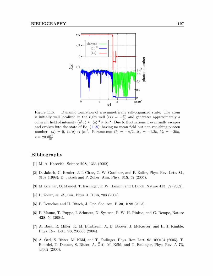
BIBLIOGRAPHY 197
Figure 11.5. Dynamic formation of a symmetrically self-organized state. The atomis initially well localized in the right well (〈x〉 = − π
2 ) and generates approximately a
coherent field of intensity⟨
a†a⟩
≈ |〈a〉|2 ≈ |α|2. Due to fluctuations it eventually escapesand evolves into the state of Eq. (11.8), having no mean field but non-vanishing photonnumber: 〈a〉 = 0,
⟨
a†a⟩
≈ |α|2. Parameters: U0 = −κ/2, ∆c = −1.2κ, V0 = −2~κ,
κ ≈ 200~k2
m .
Bibliography
[1] M. A. Kasevich, Science 298, 1363 (2002).
[2] D. Jaksch, C. Bruder, J. I. Cirac, C. W. Gardiner, and P. Zoller, Phys. Rev. Lett. 81,3108 (1998); D. Jaksch and P. Zoller, Ann. Phys. 315, 52 (2005).
[3] M. Greiner, O. Mandel, T. Esslinger, T. W. Hansch, and I. Bloch, Nature 415, 39 (2002).
[4] P. Zoller, et. al., Eur. Phys. J. D 36, 203 (2005).
[5] P. Domokos and H. Ritsch, J. Opt. Soc. Am. B 20, 1098 (2003).
[6] P. Maunz, T. Puppe, I. Schuster, N. Syassen, P. W. H. Pinkse, and G. Rempe, Nature428, 50 (2004).
[7] A. Boca, R. Miller, K. M. Birnbaum, A. D. Boozer, J. McKeever, and H. J. Kimble,Phys. Rev. Lett. 93, 233603 (2004).
[8] A. Ottl, S. Ritter, M. Kohl, and T. Esslinger, Phys. Rev. Lett. 95, 090404 (2005); T.Bourdel, T. Donner, S. Ritter, A. Ottl, M. Kohl, and T. Esslinger, Phys. Rev. A 73,43602 (2006).

198 Publication: Entanglement Assisted Fast Reordering of Atoms . . .
[9] C. Maschler and H. Ritsch, Phys. Rev. Lett. 95, 260401 (2005); C. Maschler and H.Ritsch, Opt. Comm. 243, 145 (2004).
[10] S. Zippilli and G. Morigi, Phys. Rev. Lett. 95, 143001 (2005); ibid., Phys. Rev. A 72,053408 (2005).
[11] A. Vukics, J. Janszky, and P. Domokos, J. Phys. B. 38, 1453 (2005).
[12] P. Domokos and H. Ritsch, Phys. Rev. Lett. 89, 253003 (2002).
[13] A. T. Black, H. W. Chan, and V. Vuletic, Phys. Rev. Lett. 91, 203001 (2003).
[14] J. K. Asboth, P. Domokos, H. Ritsch, and A. Vukics, Phys. Rev. A 72, 053417 (2005).
[15] S. Inouye, A. P. Chikkatur, D. M. Stamper-Kurn, J. Stenger, D. E. Pritchard, and W.Ketterle, Science 285, 571 (1999), and references therein.
[16] S. Lloyd, Phys. Rev. A 62, 022108 (2000).
[17] C. Cohen Tannoudji, Atoms in electromagnetic fields, World Scientific Singapore, 1994.
[18] A. V. Rau, J. A. Dunningham, and K. Burnett, Science 301, 1081 (2003).
[19] G. Vidal and R. F. Werner, Phys. Rev. A 65, 032314 (2002).
Chapter 12
Publication
Microscopic Physics of Quantum Self-Organisation of Optical
Lattices in Cavities†
New Journal of Physics 9, 255 (2007)
A. Vukics, C. Maschler, and H. Ritsch
Institut fur theoretische Physik, Universitat Innsbruck,A-6020 Innsbruck, Austria
We study quantum particles at zero temperature in an optical lattice coupled to aresonant cavity mode. The cavity field substantially modifies the particle dynamics in thelattice, and for strong particle-field coupling leads to self-organisation of the particles, aconfiguration with only every second site occupied. We study the growth of this order outof a homogeneous initial distribution for few particles. Simulations reveal that the growthdynamics crucially depends on the initial quantum many-body state of the particles andcan be monitored via the cavity fluorescence. Studying the relaxation time of the orderingreveals inhibited tunneling due to the interaction with the cavity field. However, therelaxation becomes very quick for strong coupling.
12.1 Introduction
Ultracold atoms in an optical lattice formed by a far detuned laser field constitute an idealsystem to study quantum phase transitions, i.e., phase transitions at zero temperature [1]. Inthe most prominent example first predicted theoretically [2] and confirmed experimentally [3]it was found that the particle ground state changes from a superfluid state where all atomsare delocalised to a perfectly ordered Mott insulator state for increasing lattice depth. Morecomplex phases as supersolids, etc. were predicted if long range interactions or mixed speciessetups [4, 5] are used, but these are harder to realize and measure experimentally. While thefinal states are well understood, these phase transitions require the buildup or decay of longrange correlations, the mechanism and time scale of which is not fully understood.
In a parallel development a dynamical transition to a self-organised phase in opticallattices was found for classical particles, when the lattice is placed inside an optical resonator.
†The primary contribution of the author of the present thesis to this publication were all the calculationsconcerning the Bose-Hubbard model. He also acted as a discussion partner for all the aspects of this work.
200 Publication: Microscopic Physics of Quantum Self-Organisation . . .
It originates from interference of the resonantly enhanced light field scattered by the atomsinto the cavity mode with the lattice light itself and leads to a preferred occupation of everysecond site [6]. For a finite temperature cloud thermal density fluctuations are amplified andlead to a runaway self-organisation by feedback from the cavity field. However, for a BEC(T ≈ 0) the initial density is perfectly homogeneous and only quantum fluctuations whichgo beyond a mean field description of the cold gas can start the self-organising process whenthe cavity interaction is switched on. Tunnelling results in a dynamical change of the atomicphase at T = 0 which gets irreversible only if cavity decay is included. In this work we studythis quantum dynamics on the microscopic level and show how it depends on the precisequantum properties of the initial atomic state beyond any mean field density.
The paper is also intended to show the limitations of the effective Bose-Hubbard typemodel developed earlier [7] for atom-cavity systems. We demonstrate that in the regimeof moderate coupling the low-dimensional Bose-Hubbard approach reproduces very well theresults of a full Monte Carlo wave-function simulation, while it breaks down in the regime ofstronger coupling. Even in this regime, however, it predicts the steady state surprisingly well,whereas the relaxation time to this state is predicted wrong. We show that the relaxationtime of the system exhibits a highly non-trivial behaviour. In the regime of moderate atom-cavity coupling the relaxation time is composed of the timescale of photon counts and thatof tunnelling. The combination of these two time scales leads to a minimum behaviour in therelaxation time, while for stronger coupling the relaxation becomes very quick, a behaviourobserved in the full simulations but not reproducible with the Bose-Hubbard approach.
We first describe our system, the model, and solution methods applied. Afterwards, wego on investigating the dynamics of a single atom in the system. Although self-organisationcannot be defined in this case, we demonstrate that already here the relaxation time exhibitsthe same behaviour we find later for two atoms, and here it is easier to give a qualitativepicture of this behaviour. We finally turn to the case of two atoms and show how theincreasing coupling results in a transition from a T = 0 homogeneous initial condition into aself-organised configuration in steady state.
12.2 System, Models
The proposed setup is depicted in Figure 12.1. It consists of a one dimensional optical latticewithin a cavity sustaining a single mode with its axis aligned orthogonally to the latticeaxis — such systems have been studied in diverse theoretical contexts before [8–11], and areavailable experimentally [12, 13]. We assume that the cavity mode function is constant alongthe lattice direction, still, as we will see below, it modifies significantly the dynamics of atomsin the lattice.
A standard quantum optical model for the system with a single atom moving in onedimension along the lattice axis is obtained by adiabatic elimination of the atomic excitedstate(s). This is justified in the regime where the driving — in our case, the laser generatingthe lattice (pump) — is far detuned from the atomic transition frequency [14, 15]. TheHamiltonian for a single atom and the cavity then reads (~ = 1):
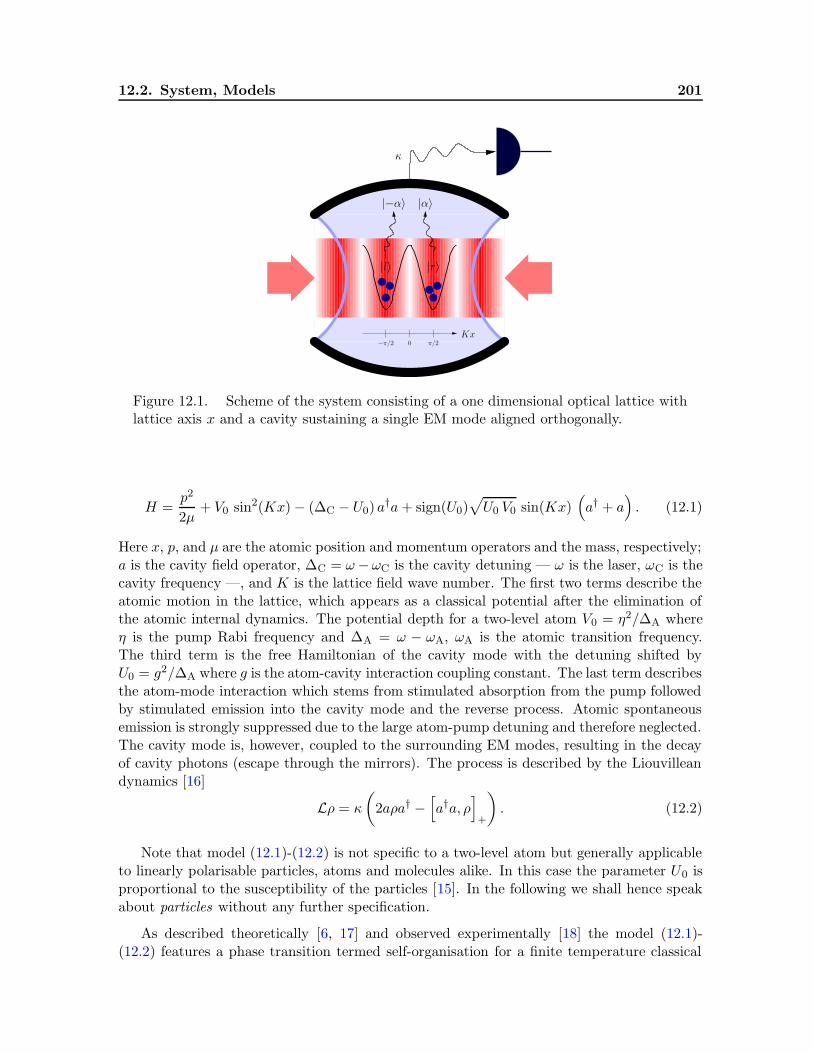
12.2. System, Models 201
κ
|l〉 |r〉
Kx−π/2 0 π/2
|−α〉 |α〉
Figure 12.1. Scheme of the system consisting of a one dimensional optical lattice withlattice axis x and a cavity sustaining a single EM mode aligned orthogonally.
H =p2
2µ+ V0 sin2(Kx)− (∆C − U0) a
†a+ sign(U0)√
U0 V0 sin(Kx)(
a† + a)
. (12.1)
Here x, p, and µ are the atomic position and momentum operators and the mass, respectively;a is the cavity field operator, ∆C = ω−ωC is the cavity detuning — ω is the laser, ωC is thecavity frequency —, and K is the lattice field wave number. The first two terms describe theatomic motion in the lattice, which appears as a classical potential after the elimination ofthe atomic internal dynamics. The potential depth for a two-level atom V0 = η2/∆A whereη is the pump Rabi frequency and ∆A = ω − ωA, ωA is the atomic transition frequency.The third term is the free Hamiltonian of the cavity mode with the detuning shifted byU0 = g2/∆A where g is the atom-cavity interaction coupling constant. The last term describesthe atom-mode interaction which stems from stimulated absorption from the pump followedby stimulated emission into the cavity mode and the reverse process. Atomic spontaneousemission is strongly suppressed due to the large atom-pump detuning and therefore neglected.The cavity mode is, however, coupled to the surrounding EM modes, resulting in the decayof cavity photons (escape through the mirrors). The process is described by the Liouvilleandynamics [16]
Lρ = κ
(
2aρa† −[
a†a, ρ]
+
)
. (12.2)
Note that model (12.1)-(12.2) is not specific to a two-level atom but generally applicableto linearly polarisable particles, atoms and molecules alike. In this case the parameter U0 isproportional to the susceptibility of the particles [15]. In the following we shall hence speakabout particles without any further specification.
As described theoretically [6, 17] and observed experimentally [18] the model (12.1)-(12.2) features a phase transition termed self-organisation for a finite temperature classical

202 Publication: Microscopic Physics of Quantum Self-Organisation . . .
gas. As this occurs for red-detuned driving, i.e., high field seeking particles with U0, ∆C < 0we will restrict ourselves to this case. Self-organisation can be qualitatively understoodas follows: The system has three steady-state configurations in a mean field description:(i) an “unorganised” configuration where the particles are equally distributed through alllattice sites and scatter no light into the cavity due to destructive interference and (ii) two“organised” configurations in which the particles occupy either only the even or only the oddsites of the lattice and scatter superradiantly into the cavity. In the latter case the last termin the Hamiltonian (12.1) deepens the lattice potential at the positions of the particles, sothat they are self-trapped or “self-organised”.
Configurations (ii) have lower energy and entropy (lower symmetry) than configuration (i).At a given temperature the system chooses between configuration (i) and one of configurations(ii) so as to minimise the free energy. Lowering the temperature results in a phase transitionwhen the symmetry of configuration (i) is spontaneously broken into the lower symmetry ofone of configurations (ii).1
The above qualitative picture is modified by the fact that the system never reaches thermalequilibrium with some external heat bath as energy is continuously flowing through the systemfrom the pump via scattering on the particles into the cavity field and then out via the cavityloss channel. Self-organisation is therefore a dynamical phase transition for which the abovementioned configurations are steady-state patterns. In steady state the particles have amomentum distribution determined by the cavity field fluctuations, which, in most cases ofphysical interest, resembles very much a thermal distribution [19]. In this sense it is justifiedto speak about an effective temperature of the particles and use the picture of an equilibriumphase transition as we did above.
Let us now turn to the case of zero temperature and envisage a fixed number of classicalpoint particles at each lattice site. In contrast to above, no matter whether we are above orbelow the threshold, no dynamics will arise because a homogeneous gas scatters no field intothe cavity due to destructive interference. If no photons are present initially, such a classicalgas cannot break the symmetry and is unable to escape the initial homogeneous configuration(i).
In the following we show that this is quite different for quantum particles at T = 0, asituation which can be prepared by loading a BEC or particles coupled out from a BEC intothe cavity [20, 21]. Interestingly, in this case both for a Mott insulator and superfluid state(BEC) as initial condition, quantum fluctuations and the possibility of tunnelling betweenlattice sites immediately start self-organisation and the superradiant build-up of the cavityphoton number. This is combined with an intricate measurement-induced dynamics relatedto the information gained via the dissipation channel of the photon-loss.
Let us emphasise that there are two main differences as compared to the above-describedclassical self-organisation: the initial temperature of the particles is zero and the particlesin the lattice are confined strongly enough so that hopping between the lattice sites is duesolely to tunnelling. Redistribution thus is a coherent quantum process and requires no directinter-particle interaction.
1Note that self-organisation is a phase transition without any direct particle-particle interaction: only aneffective interaction exists generated by the single cavity mode with which all particles interact.
12.3. Discussion 203
We are using two approaches to the problem. The first one is the direct simulation of thesystem (12.1)-(12.2) by the Monte Carlo wave-function (MCWF) method, which unravels thecorresponding Master equation in terms of individual quantum trajectories. This approachtakes into account the full particle and cavity dynamics, with the cavity decay accountedfor by quantum jumps. We are using a new simulation framework presented in Reference[22]. The second approach analogous to standard Bose Hubbard models is based on a second-quantised form of the Hamiltonian (12.1):
∫
dxΨ†(x)H Ψ(x) where the field operator Ψ(x)is restricted to the lowest vibrational band of the lattice.
To obtain the smallest possible system useful for studying self-organisation, we restrictthe dynamics to only one lattice wavelength, that is, two lattice sites (cf. Figure 12.1) withperiodic boundary condition. This is the smallest system which can seize the differencebetween the configurations described above and contains all the essential physics.
With two lattice sites the lowest vibrational band constitutes a two-dimensional Hilbertspace, for which the localised Wannier basis with state |l〉 localised at the left and |r〉 at theright lattice site can be used. Hence Ψ(x) = 〈x | l〉 bl + 〈x | r〉 br, where bl and br are thecorresponding bosonic annihilation operators. Putting the restricted field operator back intothe second-quantised Hamiltonian we obtain the Bose-Hubbard type Hamiltonian:
HBH = J(
b†l br + b†rbl)
− (∆C −NU0) a†a+ J
(
b†l bl − b†rbr)(
a† + a)
, (12.3)
where J ≡ 〈l| (p2/(2µ) + V0 sin2(Kx))|r〉 and J/(sign(U0)√U0 V0) ≡ 〈l| sin(Kx)|l〉 =
−〈r| sin(Kx)|r〉.The dynamics of particles in cavities as described by such Hamiltonians in system con-
figurations different from the one investigated here has been discussed in Refs. [7, 23, 24].A very attractive feature of Hamiltonian (12.3) is that it is simple enough so that togetherwith the Liouvillean (12.2) the full time-dependent Master equation can be solved even forseveral particles. For discussions below we will imagine this Master equation as unravelledin quantum trajectories.
12.3 Discussion
Self-organisation of an initially thermal gas of classical point-like particles in the system withclassical cavity field (coherent state) has been described above to set the scene for the two-particle quantum results presented in Section 12.5, and to raise two questions concerningquantum particles in a quantum-mechanically described cavity field:
1. whether in the steady state of the quantum Master equation (12.1)-(12.2) there is sometransition, a quantum analogue for the above-described self-organisation, which is aclassical dynamical phase transition [17].
2. if there is such a transition then whether there is a mechanism via which an ultracoldhomogeneous gas can escape the unorganised configuration and evolve into the organisedone(s), which is not possible with a classical mean-field description of either the atomsor the cavity field [25].

204 Publication: Microscopic Physics of Quantum Self-Organisation . . .
In Section 12.5 both questions will be answered to the positive for the case of two particlesin the system restricted to two lattice sites, which is the smallest system for which thetwo questions make sense. For two particles we certainly cannot expect a “quantum phasetransition”. Nonetheless, we do observe a very smooth transition in the structure of thequantum steady state, which is analogous to self-organisation as it happens in the secondorder density correlation.
From the discussion in Section 12.2 we also see that unlike in the classical case, where themodel could be solved even for several thousand particles [6, 14, 17], full quantum mechanicalsolution for several particles is difficult. Indeed, to account for the dynamical nature of thelattice, i.e., the fact that the field scattered by the particles from the pump into the cavitymodifies the potential felt by the particles (cf. last term in the Hamiltonian (12.1)), severalsingle-particle states has to be incorporated in the simulation: In the MCWFS we typicallyuse 30 momentum eigenstates (for details see Reference [22]). For N particles this gives a30N dimensional Hilbert space, which is further multiplied by the cavity-field Hilbert space.With nowadays computational resources this approach can be practically pursued up to twoparticles. In the Bose-Hubbard approach, on the other hand, there are only two single-particle states, but these are defined by the lattice potential solely. Hence it remains tobe demonstrated that this approach can be applied at all to describe self-organisation, aphenomenon based on the dynamical nature of the lattice. This problem is also addressed inSection 12.5 where we compare our two-particle MCWFS and Bose-Hubbard results.
12.4 Single-particle dynamics
We first consider the dynamics of a single particle initially prepared in one of the localisedstates (say, |r〉). Without coupling to the cavity (U0 = 0) the particle moves unperturbed inthe lattice via tunnelling, which, in the case of two sites corresponds to an oscillation betweenstates |r〉 and |l〉. This can be monitored via the expectation value 〈Kx〉, which, as displayedin Figure 12.2 (a) (red line), oscillates accordingly between ±π/2 (cf. also Figure 12.1).
This simple behaviour is significantly modified in the presence of even a weakly coupledcavity, U0 6= 0. Now the particle scatters photons from the lattice field into the cavity mode,depending on its state. Photons can decay according to the Liouvillean (12.2) and allow tomonitor the particle motion. The decay of a cavity photon can be modelled by a quantumjump, which is mathematically described by the application of the cavity field operator a onthe state vector of the system. This, in turn, changes the whole particle-field wave functionand thus gives feedback on the particle localisation.
When the coupling is weak enough, the field in the cavity will be small, and the contri-bution of the last term of Hamiltonian (12.1) to the potential felt by the particle (secondterm in the same Hamiltonian) is negligible, so that it still makes sense to define the localisedparticle states solely from the lattice potential.
We assume that these states are well localised. When a point-like particle is placed intothe lattice at position x in steady state it radiates a coherent field |α(x)〉 into the cavitywhere the amplitude is determined by the Liouvillean dynamics (12.1)-(12.2) and reads
α(x) =
√U0V0
U0 −∆C − iκsin(Kx) =
√U0V0
κ
1
1− i sin(Kx), (12.4)
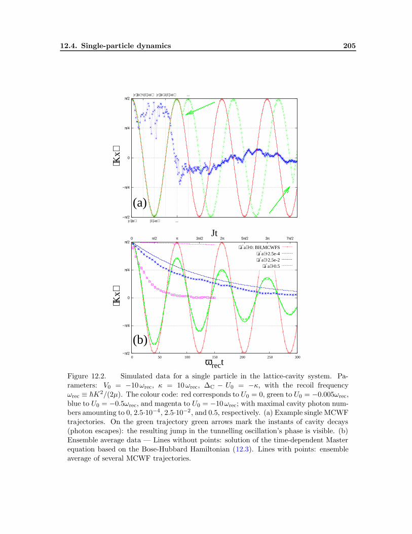
12.4. Single-particle dynamics 205
−π/2
−π/4
0
π/4
π/2
...|l⟩|-α⟩|r⟩|α⟩
...|r⟩|α⟩-i|l⟩|-α⟩|r⟩|α⟩+i|l⟩|-α⟩
⟨Kx⟩
(a)
−π/2
−π/4
0
π/4
π/2
0 50 100 150 200 250 300
7π/23π5π/22π3π/2ππ/20
⟨Kx⟩
ωrect
Jt
(b)
⟨a†a⟩=0: BH,MCWFS⟨a†a⟩=2.5e-4⟨a†a⟩=2.5e-2
⟨a†a⟩=0.5
Figure 12.2. Simulated data for a single particle in the lattice-cavity system. Pa-rameters: V0 = −10ωrec, κ = 10ωrec, ∆C − U0 = −κ, with the recoil frequencyωrec ≡ ~K2/(2µ). The colour code: red corresponds to U0 = 0, green to U0 = −0.005ωrec,blue to U0 = −0.5ωrec, and magenta to U0 = −10ωrec; with maximal cavity photon num-bers amounting to 0, 2.5·10−4, 2.5·10−2, and 0.5, respectively. (a) Example single MCWFtrajectories. On the green trajectory green arrows mark the instants of cavity decays(photon escapes): the resulting jump in the tunnelling oscillation’s phase is visible. (b)Ensemble average data — Lines without points: solution of the time-dependent Masterequation based on the Bose-Hubbard Hamiltonian (12.3). Lines with points: ensembleaverage of several MCWF trajectories.

206 Publication: Microscopic Physics of Quantum Self-Organisation . . .
where the second equality holds under the resonance condition ∆C − NU0 = −κ (N is theparticle number), to which we restrict ourselves in the following. This makes that the cavityfield increases monotonically with increasing coupling.
Accordingly, in state |r〉 the particle will radiate an approximately coherent state |α〉,while in state |l〉 a coherent state with opposite phase | − α〉, where α = α(x = π/(2K)). Itcan also be expressed from the Bose-Hubbard model as α = J/(κ(1 − i)).
If we assume that tunnelling is much slower than cavity field evolution, then the latterwill follow adiabatically the former. Without cavity jumps the system evolves coherently andsince the back action of the cavity field on the particle motion is negligible by our assumption,this evolution amounts to an oscillation between states |r, α〉 and |l,−α〉, hence at a giventime instant t the overall state of the particle-cavity system reads approximately
|Ψ(t)〉 = cos(Jt)|r, α〉 + i sin(Jt)|l,−α〉. (12.5)
Now imagine that at time t a jump happens: Immediately after the jump the state of thesystem reads
|Ψ′(t)〉 ∝ a|Ψ(t)〉 ∝ cos(Jt)|r, α〉 − i sin(Jt)|l,−α〉, (12.6)
that is, the cavity jump is reflected back onto the particle motion and results in a jump ofthe phase of the tunnelling oscillation.
This behaviour is verified by the simulations, an example trajectory is displayed in Fig-ure 12.2 (a) (green line). Here the parameters were chosen such that the maximal expectationvalue of the cavity photon number is only 2.5 · 10−4 — this maximum is achieved when theparticle is prepared perfectly localised at a lattice site.
The jump is a stochastic event and in ensemble average the jumps of the phases onindividual trajectories result in a dephasing and hence damping of the oscillation. Thisbehaviour, as displayed in Figure 12.2 (b) (green lines) is verified by both the MCWFS and thesimulation of the time-dependent Master equation based on the Bose-Hubbard Hamiltonian(12.3). In this regime of very low cavity photon number, the correspondence between thetwo models is very good. Increasing the photon number results in several jumps happeningin one tunnelling cycle: in ensemble average this corresponds to the over-damped regime ofthe tunnelling oscillation (cf. Figure 12.2 (a-b) blue line).
The above picture of the dynamics on one Monte Carlo trajectory is not valid in theregime of stronger coupling where the photon number is higher. Here the cavity field modifiessignificantly the potential felt by the particle and hence the states |r〉 and |l〉 defined solelyby the lattice potential lose their significance because many other particle spatial states enterthe dynamics. Cavity decays are much more frequent, and the stronger field fluctuations arereflected back onto the potential. Accordingly, as we observe in Figure 12.2 (magenta line),the Bose-Hubbard approach being based on those two states breaks down in this regime.
The steady state of the dynamics is, quite independently of the coupling, the mixed stateρss ≈ (|r, α〉 〈r, α|+ |l,−α〉 〈l,−α|)/2. As displayed in Figure 12.3, the relaxation time to thisstate, that is, the time scale of the damping of the tunnelling oscillation exhibits a non-trivialbehaviour. For moderate coupling, according to the discussion above, this is composed oftwo time scales: the time scale of cavity photon decay, and that of tunnelling. The formerbeing inversely proportional to the photon number gets faster with increasing coupling.

12.5. Two-particle dynamics 207
0
50
100
150
200
250
300
0.001 0.01 0.1 1 10 100
t rela
xωre
c
|U0|/ωrec
MCWFS
BH
Figure 12.3. Relaxation time of the damping of the tunnelling oscillation simulatedwith the MCWF and Bose-Hubbard approach. Same parameters as above. The dottedhyperbole has been fit on the weak-coupling part of the data and is proportional to thecavity photon count rate. The dotted horizontal line is the time scale of tunnelling withno coupling.
On the other hand the latter gets slower, a behaviour verified by both the MCWF andthe Bose-Hubbard approach. In the following we give an interpretation in the framework ofthe Bose-Hubbard approach. Here, when initially in the state |r, α〉, the system first evolvesinto |l, α〉 via tunnelling (first term of Hamiltonian (12.3)), and this state is then transformedinto |l,−α〉 by the dissipative cavity evolution on a timescale of κ−1, since in steady statethe particle in state |l〉 radiates the approximately coherent field | − α〉. States |r, α〉 and|l, α〉, however, have different energies because of the last term in Hamiltonian (12.3), sothat the tunnelling becomes non-resonant and hence slows down as compared to the free (no-cavity) case. Using the α value calculated above from the Bose-Hubbard approach the energydifference reads ∆ = 2J2/κ ∝ |U0|. With increasing U0 the energy difference increases, sothat tunnelling gets slower. The above discussion is summarised in Figure 12.4.
The combination of one accelerating and one slowing time scale results in the minimumbehaviour of the relaxation time in Figure 12.3 around U0 = −0.05ωrec. Ultimately, withhigh enough coupling the cavity-generated potential starts to dominate the lattice potential,in which regime strong fluctuations and self-trapping lead to fast relaxation as observed inthe MCWFS (red line |U0| & ωrec). Obviously, the Bose-Hubbard approach is unable toreproduce the behaviour in this regime.
12.5 Two-particle dynamics
Having understood the dissipative quantum dynamics of a single particle in our lattice-cavitysystem, we now turn to the case of two particles. Two particles on two lattice sites with
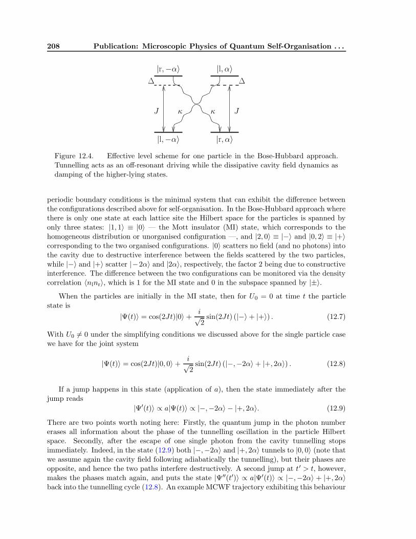
208 Publication: Microscopic Physics of Quantum Self-Organisation . . .
|l,−α〉
|l, α〉
|r, α〉
|r,−α〉
κκJ J
∆ ∆
Figure 12.4. Effective level scheme for one particle in the Bose-Hubbard approach.Tunnelling acts as an off-resonant driving while the dissipative cavity field dynamics asdamping of the higher-lying states.
periodic boundary conditions is the minimal system that can exhibit the difference betweenthe configurations described above for self-organisation. In the Bose-Hubbard approach wherethere is only one state at each lattice site the Hilbert space for the particles is spanned byonly three states: |1, 1〉 ≡ |0〉 — the Mott insulator (MI) state, which corresponds to thehomogeneous distribution or unorganised configuration —, and |2, 0〉 ≡ |−〉 and |0, 2〉 ≡ |+〉corresponding to the two organised configurations. |0〉 scatters no field (and no photons) intothe cavity due to destructive interference between the fields scattered by the two particles,while |−〉 and |+〉 scatter |−2α〉 and |2α〉, respectively, the factor 2 being due to constructiveinterference. The difference between the two configurations can be monitored via the densitycorrelation 〈nlnr〉, which is 1 for the MI state and 0 in the subspace spanned by |±〉.
When the particles are initially in the MI state, then for U0 = 0 at time t the particlestate is
|Ψ(t)〉 = cos(2Jt)|0〉 + i√2
sin(2Jt) (|−〉+ |+〉) . (12.7)
With U0 6= 0 under the simplifying conditions we discussed above for the single particle casewe have for the joint system
|Ψ(t)〉 = cos(2Jt)|0, 0〉 + i√2
sin(2Jt) (|−,−2α〉 + |+, 2α〉) . (12.8)
If a jump happens in this state (application of a), then the state immediately after thejump reads
|Ψ′(t)〉 ∝ a|Ψ(t)〉 ∝ |−,−2α〉 − |+, 2α〉. (12.9)
There are two points worth noting here: Firstly, the quantum jump in the photon numbererases all information about the phase of the tunnelling oscillation in the particle Hilbertspace. Secondly, after the escape of one single photon from the cavity tunnelling stopsimmediately. Indeed, in the state (12.9) both |−,−2α〉 and |+, 2α〉 tunnels to |0, 0〉 (note thatwe assume again the cavity field following adiabatically the tunnelling), but their phases areopposite, and hence the two paths interfere destructively. A second jump at t ′ > t, however,makes the phases match again, and puts the state |Ψ′′(t′)〉 ∝ a|Ψ′(t)〉 ∝ |−,−2α〉 + |+, 2α〉back into the tunnelling cycle (12.8). An example MCWF trajectory exhibiting this behaviour

12.5. Two-particle dynamics 209
is plotted in Figure 12.5(a) (green line). We observe that a quantum jump brings the systeminto the state (12.9), signalled by 〈nlnr〉 = 0, and it remains there until the next jump, whenit starts to oscillate anew.
In ensemble average these stochastic “dark” periods of the tunnelling oscillation lead todamping just as in the single-particle case. The final steady state is always a mixture
ρss = w|0, 0〉 〈0, 0| + 1− w2
(|−,−2α〉 〈−,−2α|+ |+, 2α〉 〈+, 2α|) . (12.10)
At this point it becomes clear that any mean-field description of this system is bound to fail:a mean cavity field description would prohibit the possibility of a coherent superposition ofdifferent particle configurations radiating different fields as in (12.8), which is essential for theonset of the dynamics from a homogeneous zero-temperature initial condition (see also [25]).On the other hand, a particle mean field cannot seize the difference between states (12.10)with different w, because this appears only in the density correlation.
As displayed in Figure 12.5 (b), our two approaches for simulating the damping agreewell in the regime of moderate coupling. However, just as in the single-particle case, strongcoupling — in the regime where the cavity-generated potential dominates the lattice one— results in extremely quick damping, which cannot be reproduced by the Bose-Hubbardapproach. Here the relaxation time exhibits the same behaviour as we have seen in thesingle-particle case (cf. Figure 12.6 (a)): with increasing coupling it has a minimum, afterwhich the Bose-Hubbard approach gives a monotonic increase of the relaxation time, whilethe MCWFS gives a peak, and for even stronger coupling very quick relaxation. For theinterpretation of this behaviour the same discussion applies as above for the single-particlecase.
Increasing coupling results in a decrease of the weight w of the MI component in steadystate, cf. Figure 12.6 (b), and with strong enough coupling (|U0| & 10ωrec in our case)the steady state is confined solely into the self-organised subspace. This proves our initialassertion that even when the system is started from a T = 0 homogeneous state (here theMI state) self-organisation can occur. On the same Figure we also see that this is confirmedby both approaches, only the relaxation time of the process is predicted wrongly by theBose-Hubbard approach for strong coupling.
It is easy to see that starting the system from the superfluid (SF) state
|SF〉 ∝ |0〉+ 1√2
(|−〉+ |+〉) (12.11)
instead of the MI as above does not change the steady state since already the first quantumjump erases the information about the initial condition completely. The process of relaxationwill, however, be different. This process can be monitored by a time resolved analysis ofthe intensity escaping the cavity, which is proportional to the cavity photon number: anexample is displayed in Figure 12.7. Here, we are in the over-damped regime of the tunnellingoscillation. When prepared in the MI state, the particles do not scatter initially, and thebuildup of the cavity field occurs on the time scale of the self-organisation process. With theSF initial state, on the other hand, some field is built up almost instantly (on the time scaleof κ−1), because in the SF the states |±〉 have finite weight; while the rest of the field is builtup on the longer time scale.

210 Publication: Microscopic Physics of Quantum Self-Organisation . . .
1(MI)
0.75
0.5(SF)
0.25
0(SO)
432Jump 1
⟨nln
r⟩
(a)
1(MI)
0.75
0.5(SF)
0.25
0(SO) 0 50 100 150 200
2π3π/2ππ/20
⟨nln
r⟩
ωrect
Jt
(b)⟨a†a⟩=0: BH,MCWFS
⟨a†a⟩=1e-3⟨a†a⟩=0.1
⟨a†a⟩=2
Figure 12.5. Simulated data for two particles in the lattice-cavity system with sameparameters as above. The colours correspond to the same values of U0, here with maximalcavity photon numbers amounting to 0, 10−3, 0.1, and 2. (a) Example single MCWFtrajectories — the vertical dotted lines mark the time instants of cavity decays on thetrajectory plotted in green. (b) Ensemble average data — lines without points: datastemming from the Bose-Hubbard approach; lines with points: MCWF approach.
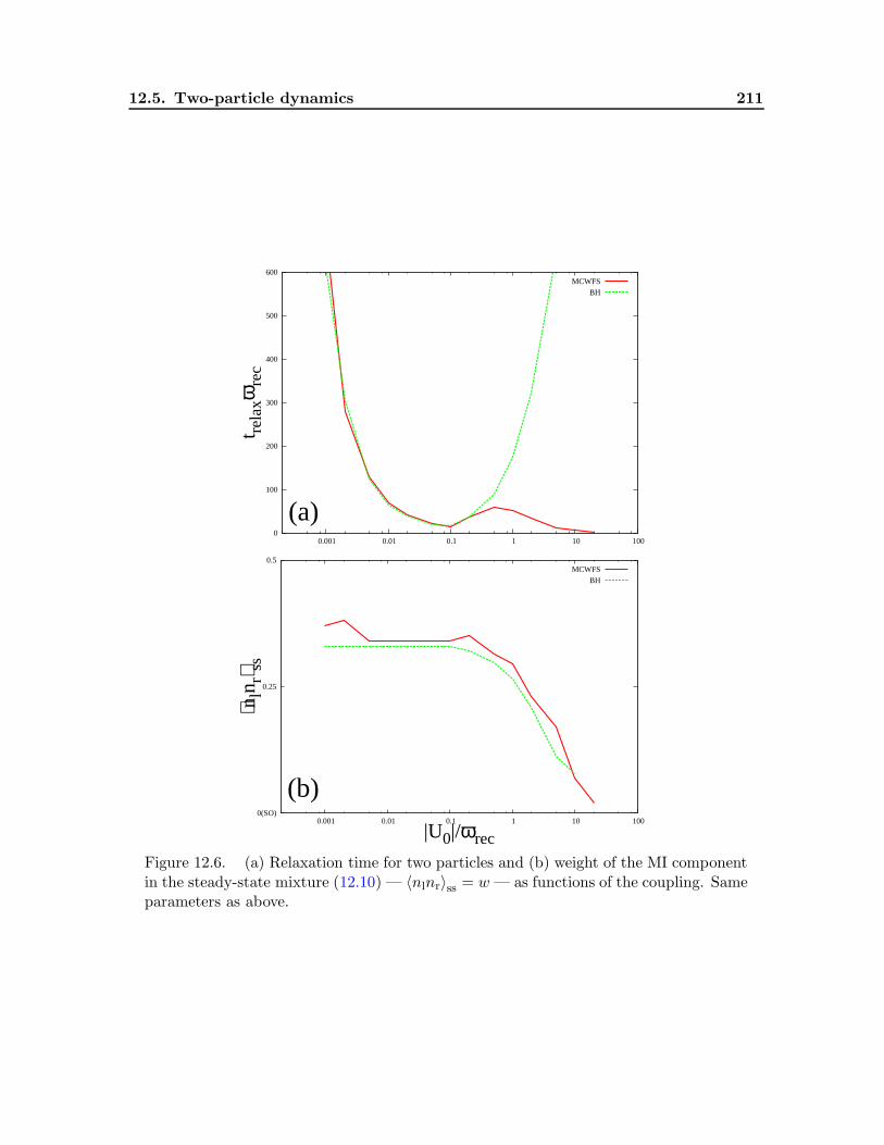
12.5. Two-particle dynamics 211
0
100
200
300
400
500
600
0.001 0.01 0.1 1 10 100
t rela
xωre
c
(a)
MCWFS
BH
0.5
0.25
0(SO) 0.001 0.01 0.1 1 10 100
⟨nln
r⟩ ss
|U0|/ωrec
(b)
MCWFS
BH
Figure 12.6. (a) Relaxation time for two particles and (b) weight of the MI componentin the steady-state mixture (12.10) — 〈nlnr〉ss = w — as functions of the coupling. Sameparameters as above.

212 Publication: Microscopic Physics of Quantum Self-Organisation . . .
0
0.2
0.4
0.6
0.8
1
1.2
1.4
1.6
0 5 10 15 20 25 30 35
350300250200150100500
phot
on n
umbe
r
ωrect
κt
Mott insulator
Superfluid
Figure 12.7. Initial build-up of the cavity photon number with the particles preparedinitially in the Mott insulator or superfluid state. U0 = −10ωrec, other parameters arethe same as above.
12.6 Conclusions
In summary, we have seen that coupling two particles in an optical lattice to a cavity inducesan irreversible reorganisation of the particles, a process which can be monitored directly inan experiment by the time-resolved analysis of the intensity escaping the cavity. We haveshown that no classical or mean-field description of either the particles or the cavity fieldcan account for the phenomenon. For strong enough coupling the process leads to a fastself-organisation of the particles, a configuration in which they occupy every second site inthe lattice, and scatter superradiantly into the cavity. An important conclusion of the workis that while an effective low-dimensional Bose-Hubbard type model cannot reproduce thetime evolution in the strong-coupling regime as observed in more detailed simulations, it canstill predict the steady state remarkably well. This model can therefore be used in the futurefor a high number of particles to study possible quantum phase transitions occurring in thesteady state of this dissipative system.
Bibliography
[1] S. Sachdev, Quantum Phase Transitions, (Cambridge University Press, 1999).
[2] D. Jaksch, C. Bruder, J. I. Cirac, C. W. Gardiner, and P. Zoller, Phys. Rev. Lett. 813108 (1998).
[3] M. Greiner, O. Mandel, T. Esslinger, T. W. Hansch, and I. Bloch, Nature 415, 39 (2002).
[4] H. P. Buchler and G. Blatter, Phys. Rev. Lett. 91, 130404 (2003).
[5] V. W. Scarola, E. Demler, and S. Das Sarma, Phys. Rev. A 73, 051601(R) (2006).
BIBLIOGRAPHY 213
[6] P. Domokos and H. Ritsch, Phys. Rev. Lett. 89, 253003 (2002).
[7] C. Maschler and H. Ritsch, Phys. Rev. Lett. 95, 260401 (2005).
[8] P. Domokos, A. Vukics, and H. Ritsch, Phys. Rev. Lett. 92, 103601 (2004).
[9] S. Zippilli and G. Morigi, Phys. Rev. Lett. 95, 143001 (2005).
[10] J. Metz, M. Trupke, and A. Beige, Phys. Rev. Lett. 97, 040503 (2006).
[11] K. Murr, Phys. Rev. Lett. 96, 253001 (2006).
[12] B. Nagorny, T. Elsasser, and A. Hemmerich, Phys. Rev. Lett. 91, 153003 (2003).
[13] S. Nussmann et al., Nat. Phys. 1, 122 (2005).
[14] P. Domokos and H. Ritsch, J. Opt. Soc. Am. B 20, 1098 (2003).
[15] A. Vukics and P. Domokos, Phys. Rev. A 72, 031401 (2005).
[16] C. W. Gardiner and P. Zoller, Quantum Noise, 2nd Ed., (Springer, Berlin, 2000).
[17] J. K. Asboth, P. Domokos, H. Ritsch, and A. Vukics, Phys. Rev. A 72, 053417 (2005).
[18] A. T. Black, H. W. Chan, and V. Vuletic, Phys. Rev. Lett. 91, 203001 (2003).
[19] A. Vukics, J. Janszky, and P. Domokos, J. Phys. B 38, 1453 (2005).
[20] A. Ottl, S. Ritter, M. Kohl, and T. Esslinger, Phys. Rev. Lett. 95, 090404 (2005).
[21] A. Ottl, S. Ritter, M. Kohl, and T. Esslinger, Rev. Sci. Instrum. 77, 063118 (2006).
[22] A. Vukics and H. Ritsch, Eur. Phys. J. D (to be published). [accepted for publication]
[23] C. Maschler and H. Ritsch, Opt. Commun. 243, 145 (2004).
[24] J. Larson, B. Damski, G. Morigi, and M. Lewenstein, cond-mat/0608335.
[25] C. Maschler, H. Ritsch, A. Vukics, and P. Domokos, Opt. Commun. 273, 446 (2007).


Curriculum Vitae
Christoph Maschler,October 2007
General
Current Address: Institute for Theoretical Physics, University of Innsbruck,Technikerstraße 25, A-6020 Innsbruck, Austria.
Date of Birth: 7th July, 1975.Place of Birth: A-6511 Zams, Austria.Citizenship: AustrianLanguages Spoken: German (Native), English (Fluent), French (Basic knowledge)
Elementary Education
1981 - 1985 Elementary School, Zams, Austria.1985 - 1993 High School, Landeck, Austria.
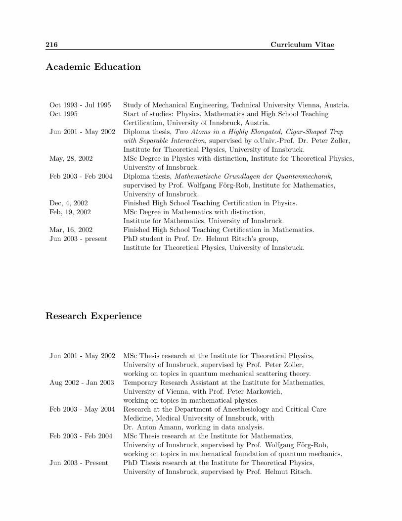
216 Curriculum Vitae
Academic Education
Oct 1993 - Jul 1995 Study of Mechanical Engineering, Technical University Vienna, Austria.Oct 1995 Start of studies: Physics, Mathematics and High School Teaching
Certification, University of Innsbruck, Austria.Jun 2001 - May 2002 Diploma thesis, Two Atoms in a Highly Elongated, Cigar-Shaped Trap
with Separable Interaction, supervised by o.Univ.-Prof. Dr. Peter Zoller,Institute for Theoretical Physics, University of Innsbruck.
May, 28, 2002 MSc Degree in Physics with distinction, Institute for Theoretical Physics,University of Innsbruck.
Feb 2003 - Feb 2004 Diploma thesis, Mathematische Grundlagen der Quantenmechanik,supervised by Prof. Wolfgang Forg-Rob, Institute for Mathematics,University of Innsbruck.
Dec, 4, 2002 Finished High School Teaching Certification in Physics.Feb, 19, 2002 MSc Degree in Mathematics with distinction,
Institute for Mathematics, University of Innsbruck.Mar, 16, 2002 Finished High School Teaching Certification in Mathematics.Jun 2003 - present PhD student in Prof. Dr. Helmut Ritsch’s group,
Institute for Theoretical Physics, University of Innsbruck.
Research Experience
Jun 2001 - May 2002 MSc Thesis research at the Institute for Theoretical Physics,University of Innsbruck, supervised by Prof. Peter Zoller,working on topics in quantum mechanical scattering theory.
Aug 2002 - Jan 2003 Temporary Research Assistant at the Institute for Mathematics,University of Vienna, with Prof. Peter Markowich,working on topics in mathematical physics.
Feb 2003 - May 2004 Research at the Department of Anesthesiology and Critical CareMedicine, Medical University of Innsbruck, withDr. Anton Amann, working in data analysis.
Feb 2003 - Feb 2004 MSc Thesis research at the Institute for Mathematics,University of Innsbruck, supervised by Prof. Wolfgang Forg-Rob,working on topics in mathematical foundation of quantum mechanics.
Jun 2003 - Present PhD Thesis research at the Institute for Theoretical Physics,University of Innsbruck, supervised by Prof. Helmut Ritsch.
217
Teaching Experience
Oct 1997 - Jan 1998 Tutor, Institute for Mathematics, University of Innsbruck.Tutor for “Analysis 1”.
Mar 1998 - Jul 1998 Tutor, Institute for Mathematics, University of Innsbruck.Tutor for “Analysis 2”.
Oct 1998 - Jan 1999 Tutor, Institute for Mathematics, University of Innsbruck.Tutor for “Mathematics for Physicists”.
Mar 1999 - Jul 1999 Tutor, Institute for Mathematics, University of Innsbruck.Tutor for “Mathematics for Physicists 2”.
Oct 1999 - Jan 2000 Tutor, Institute for Theoretical Physics, University of Innsbruck.Tutor for “Electrodynamics”.
Mar 2000 - Jul 2000 Tutor, Institute for Theoretical Physics, University of Innsbruck.Tutor for “Theoretical Mechanics”.
Oct 2000 - Jan 2001 Tutor, Institute for Theoretical Physics, University of Innsbruck.Tutor for “Thermodynamics”.
Oct 2004 - Jan 2005 Tutor, Institute for Theoretical Physics, University of Innsbruck.Tutor for “Quantum Mechanics 2”.
Mar 2005 - Jul 2005 Tutor, Institute for Theoretical Physics, University of Innsbruck.Tutor for “Theoretical Physics 3”.
Oct 2005 - Jan 2006 Tutor, Institute for Theoretical Physics, University of Innsbruck.Tutor for “Introduction to Theoretical Physics”.
Sep 2006 - Jul 2007 High School Teacher, HTL Anichstraße, Innsbruck.Teacher for “Electrical Engineering” and “Applied Mathematics”.
Preprints
1. C. Maschler, I. B. Mekhov, and H. Ritsch, Ultracold Atoms in Optical Lattices Generatedby Quantized Light Fields, arXiv: quant-ph/0710.4220.
Publications - Articles
1. C. Maschler and H. Ritsch, Quantum Motion of Laser-Driven Atoms in a Cavity Field,Opt. Comm. 243, 145 - 155 (2004).
2. C. Maschler and H. Ritsch, Cold Atom Dynamics in a Quantum Optical Lattice Poten-tial, Phys. Rev. Lett. 95, 260401 (2005).
3. C. Maschler, H. Ritsch, A. Vukics, and P. Domokos, Entanglement Assisted Fast Re-ordering of Atoms in an Optical Lattice within a Cavity at T = 0, Opt. Comm. 273,446 - 450 (2007).
4. I. B. Mekhov, C. Maschler, and H. Ritsch, Cavity Enhanced Light Scattering in OpticalLattices to Probe Atomic Quantum Statistics, Phys. Rev. Lett. 98, 100402 (2007).

218 Curriculum Vitae
5. I. B. Mekhov, C. Maschler, and H. Ritsch, Probing Quantum Phases of Ultracold Atomsin Optical Lattices by Transmission Spectra in Cavity QED, Nature Physics 3, 319 -323 (2007).
6. A. Vukics, C. Maschler, and H. Ritsch, Microscopic Physics of Quantum Self-Organisation of Optical Lattices in Cavities, New J. Phys. 9, 255 (2007).
7. I. B. Mekhov, C. Maschler, and H. Ritsch, Light Scattering from Ultracold Atoms inOptical Lattices as an Optical Probe of Quantum Statistics, Phys. Rev. A (in press).
Publications - MSc Thesis
1. C. Maschler, Two Atoms in a Highly Elongated, Cigar-Shaped Trap with SeparableInteraction, MSc Thesis for Physics, University of Innsbruck, May 2002.
2. C. Maschler, Mathematische Grundlagen der Quantenmechanik, MSc Thesis for Math-ematics, University of Innsbruck, February 2004.
Conference Contributions
• Meeting of the Spezialforschungsbereich (SFB) for Control and Measurement of Coher-ent Quantum Systems,Innsbruck, Austria, February 2002.
• 54th Annual Meeting of the Austrian Society of Physics (OPG),Linz, Austria, September 2004.
• 11th Young Atom Opticians (YAO) Conference,Hannover, Germany, February 2005.
• Obergurgl Quantum Optics Meeting 2005,Obergurgl, Austria, March 2005.
• 55th Annual Meeting of the Austrian Society of Physics (OPG),Vienna, Austria, September 2005.
• 3rd International Workshop on the Theory of Quantum Gases and Quantum Coherence,Cortona, Italy, November 2005.
• 2nd Term-Review of the Spezialforschungsbereich (SFB) for Control and Measurementof Coherent Quantum Systems,Innsbruck, Austria, January 2006.
• 20th International Conference on Atomic Physics (ICAP 2006),Innsbruck, Austria, July 2006.
219
• QUROPE Winter School on Quantum Information: Ensemble-based Quantum Infor-mation Processing,Obergurgl, Austria, February 2007.
• AMOP Spring Conference of the German Physical Society (DPG),Dusseldorf, Germany, March 2007.
• Workshop on Quantum Engineering with Neutral Atoms and Light,Herrsching am Ammersee, Germany, June 2007.
• d-fine’s Science in Finance Workshop,Schlosshotel Kronberg, Germany, October 2007.


![Workshop on Quantum Simulations with Ultracold Atomspeople.sissa.it/~andreatr/WORKSHOP_QUANTUM_SIMULATIONS...synthetic gauge potentials for cold atoms in optical lattices [1,2,3]](https://img.pdfslide.net/doc/110x75/60dd079a657564360213b425/workshop-on-quantum-simulations-with-ultracold-andreatrworkshopquantumsimulations.jpg)