Ultrasonic Non-Destructive Evaluation: ImpactPoint Prediction and Simulation of Ultrasonic Fields

Item Type text; Electronic Dissertation

Authors Hajzargarbashi, Talieh

Publisher The University of Arizona.

Rights Copyright © is held by the author. Digital access to this materialis made possible by the University Libraries, University of Arizona.Further transmission, reproduction or presentation (such aspublic display or performance) of protected items is prohibitedexcept with permission of the author.

Download date 26/05/2018 21:33:57

Link to Item http://hdl.handle.net/10150/203430

ULTRASONIC NON-DESTRUCTIVE EVALUATION: IMPACT POINT

PREDICTION AND SIMULATION OF ULTRASONIC FIELDS

by

Talieh Hajzargarbashi

_____________________

A Dissertation Submitted to the Faculty of the

DEPARTMENT OF CIVIL ENGINEERING AND ENGINEERING

MECHANICS

In Partial Fulfillment of the Requirements

For the Degree of

DOCTOR OF PHILOSOPHY

WITH A MAJOR IN ENGINEERING MECHANICS

In the Graduate College

THE UNIVERSITY OF ARIZONA

2011

2

2

THE UNIVERSITY OF ARIZONA

GRADUATE COLLEGE

As members of the Dissertation Committee, we certify that we have read the dissertation

prepared by Talieh Hajzargarbashi

entitled ULTRASONIC NON-DESTRUCTIVE EVALUATION: IMPACT POINT

PREDICTION AND SIMULATION OF ULTRASONIC FIELDS

and recommend that it be accepted as fulfilling the dissertation requirement for the

Degree of Doctor of Philosophy

_______________________________________________________________________ Date: 11/21/11

Dr. Tribikram Kundu

_______________________________________________________________________ Date: 11/21/11

Dr. George Frantziskonis

_______________________________________________________________________ Date: 11/21/11

Dr. Lianyang Zhang

_______________________________________________________________________ Date:

_______________________________________________________________________ Date:

Final approval and acceptance of this dissertation is contingent upon the candidate’s

submission of the final copies of the dissertation to the Graduate College.

I hereby certify that I have read this dissertation prepared under my direction and

recommend that it be accepted as fulfilling the dissertation requirement.

________________________________________________ Date:

Dissertation Director:

3

STATEMENT BY AUTHOR

This dissertation has been submitted in partial fulfillment of requirements for an

advanced degree at the University of Arizona and is deposited in the University Library

to be made available to borrowers under rules of the Library.

Brief quotations from this dissertation are allowable without special permission, provided

that accurate acknowledgment of source is made. Requests for permission for extended

quotation from or reproduction of this manuscript in whole or in part may be granted by

the author.

SIGNED: Talieh Hajzargarbashi

4

ACKNOWLEDGEMENTS

I would like to express my deepest gratitude to my advisor, Professor Tribikram Kundu

of the Department of Civil Engineering and Engineering Mechanics, University of

Arizona, for giving me the opportunity to work with him, and his invaluable guidance. I

also thank him for sharing his inspiring work ethic, and for showing me how to be a good

educator.

I am grateful to the members of my research committee, Prof. George Frantziskonis,

Prof. Lianyang Zhang ,Prof. John M. Kemeny and Prof. Hamid Saadatmanesh for their

comments which helped me improve this work.

My sincere thanks always remain with my remarkable friends for always being there, as

well as for constant entertaining moments we shared throughout the years.

I thank my parents, my parents-in-law, my sister, brother and my brother-in-law. Without

their never-ending love and support, I would not be where I am today.

Finally, I would like to express my deepest appreciation to my husband for his

continuous inspiration and support.

5

DEDICATION

This dissertation is dedicated to my husband, Davoud Zamani. I give my deepest

expression of love and appreciation for the encouragement that he gave and the sacrifices

he made during this graduate program.

6

TABLE OF CONTENTS

ABSTRACT…………………………………………………………………7

CHAPTER I:.INTRODUCTION………………………………………........9

Objective…..………………………………………………………….10

Background……...…………………………………………………….11

CHAPTER II: PRESENT STUDY…………………………………….…..18

REFERENCES………………….………………………………………….21

APPENDIX A: AN IMPROVED ALGORITHM FOR DETECTING

POINT OF IMPACT IN ANISOTROPIC INHOMOGENEOUS

PLATES…………………………………………...………………………25

APPENDIX B: DETECTING THE POINT OF IMPACT ON A

CYLINDRICAL PLATE BY THE ACOUSTIC EMISSION

TECHNIQUE…………… ……………………………………………........48

APPENDIX C: DETECING THE POINT OF IMPACT ON AN

ANISOTROPIC CYLINDRICAL SURFACE USING ONLY FOUR

ACOUSTIC SENSORS………………... …………………………………..61

APPENDIX D: IMPACT LOCALIZATION ON A CYLIDRICAL PLATE

BY NEAR-FIELD BEAMFORMING ANALYSIS ……………………….72

APPENDIX E: SCATTERING OF FOCUSED ULTRASONIC BEAMS BY

TWO SPHERICAL CAVITIES IN CLOSE PROXIMITY………………....85

7

ABSTRACT

This work has two parts. The first part of the work (in Chapters II, III, IV and V) presents

a method for locating the point of impact using acoustic emission techniques.

The second part of the work is modeling the ultrasonic fields generated by one and two

spherical cavities placed in front of a point focused acoustic lens using the semi-

analytical distributed point source method (DPSM).

Acoustic emission (AE) refers to the generation of transient elastic waves during the

rapid release of energy from localized sources within a material.

In this work the acoustic emission has been used for locating the point of impact on

anisotropic and homogeneous or non-homogenous flat plates and cylindrical structures.

In these cases the wave speed is a function of the angle of propagation. An optimization

function is introduced and minimized to get the location of the impact point.

This method has been used on a flat FRP (fiber reinforced polymer) plate. The proposed

new objective function reduces the amount of time needed for solving the problem and

improves the accuracy of prediction. After solving the flat plate problem the method is

extended to cylindrical structures for which the objective function is written in cylindrical

coordinates and the method is tested on a FRP shell.

In Chapter IV an alternative method is introduced called the near-field acoustic emission

(AE) beamforming method. It has been used to estimate the source locations by using a

8

small array of sensors closely placed in a local region. To validate the effectiveness of the

AE beamforming method a series of experiments on a FRP shell are conducted. The

experimental results demonstrate that the proposed method can correctly predict the point

of impact.

The semi-analytical mesh-free technique DPSM is then used to model the ultrasonic field

in front of a point focused acoustic lens; anomalies such as cavities are introduced in the

medium in front of the acoustic lens and the effect of those cavities are studied. Solution

of this problem is necessary to get an idea about when two cavities placed in close

proximity can be distinguished by an acoustic lens and when it is not possible.

9

CHAPTER I

INTRODUCTION

10

1. Objective:

Objectives of this research are two folds - first to develop an acoustic emission technique

for localizing acoustic source in anisotropic plates and shells, and then to develop a semi-

analytical model to study the scattering of ultrasonic waves by spherical cavities in a

focused ultrasonic field.

The first part of this work presents the theory and experimental results for localizing the

point of impact in isotropic and anisotropic plates and shells by the acoustic emission

technique. Localizing the point of impact on an anisotropic structure is necessary for

detecting and repairing the delamination and other type of damage arising from an

impact. Anisotropic plates and shells made of fiber reinforced composites are being

increasingly used in various structures due to their superior stiffness and light weight

characteristics. Shock, impact, or repeated cyclic stresses can cause the laminate to

separate at the interface between two layers, a condition known as delamination.

Individual fibers can separate from the matrix e.g. fiber pull-out. In order to prevent such

incidents there is always a need to identify the location of the damage prior to failure.

The second part of this work presents a formulation based on the distributed point source

method for solving elastic wave scattering problems in presence of cavities in front of an

acoustic lens. The propagation of waves through a medium containing strong scatterers is

ubiquitous in nature. This is because generally inhomogeneities are always found in

materials. These inhomogeneities locally change the acoustic properties of the material.

11

Air cavities and solid inclusions in molten and solid metals are some examples of these

inhomogeneities. A large number of papers have been published on elastic wave

propagation through materials containing inclusions. In particular, scattering of elastic

waves by spherical inhomogeneities_(e.g. voids, inclusions and other types of defect) has

been investigated because of its importance in nondestructive testing and exploratory

geophysics. Detection and characterization of floating cavities in a liquid medium is

important for both materials science and medical applications, such as for characterizing

air bubbles in molten metal and blood.

2. Background

A popular method for detecting the point of impact is the acoustic emission technique.

Acoustic emission (AE) refers to the generation of transient elastic waves during the

rapid release of energy from localized sources within a material [1]. Since AE signals

usually arise from internal changes of a structure, such as crack growth, dislocation

movement in monolithic materials, fiber breakage, fiber-matrix debonding and impact of

foreign objects, AE technique is used as a non-destructive testing tool to localize and

evaluate structural damage [2,3]. Due to its potential advantages in Kinematic damage

monitoring and source localization, AE technique has led to many applications in a

variety of fields such as petrochemical industry, aerospace industry, material,

manufacturing processes, etc [4,5].

12

Anisotropic plates and shells such as fiber reinforced composites are being increasingly

used in various structures due to their superior stiffness and weight characteristics. Shock,

impact, or repeated cyclic stresses can cause the laminate to separate at the interface

between two layers, a condition known as delamination. Individual fibers can separate

from the matrix e.g. fiber pull-out. The best known failure of a brittle ceramic matrix

composite occurred when the composite tile on the leading edge of the wing of the Space

Shuttle Columbia fractured due to impact during take-off. It led to catastrophic failure of

the vehicle when it re-entered the Earth's atmosphere on February 1, 2003. In order to

prevent such incidents there is always a need to identify the location of the damage prior

to failure. As mentioned above one of the most important reasons for the composite

damage is impact load or foreign objects striking the composite structure.

Localizing the source of the damage or the damage initiation point is very important for

health monitoring of structures. Time difference of arrival is a conventional AE method

that has been validated in laboratory settings and has become the most popular tool to

estimate the AE source location. This technique has been mostly used for isotropic plates.

Using passive sensors attached to the isotropic plate the point of impact can be localized

by the acoustic emission method following the triangulation technique [6,7]. For

efficiently monitoring the plate the sensors need to be placed near the critical locations of

the plate [8-11]. After receiving the impact generated acoustic signals at three sensor

locations the triangulation technique is applied to detect the impact point in isotropic

plates. In anisotropic plates the wave speed is not the same in all directions and therefore

the triangulation technique does not work [12, 13, 14]. Previous efforts for locating the

13

acoustic emission source in anisotropic plates required the measurement of two dominant

pulses in a waveform whose speeds of propagation c1 and c2 were known. In that earlier

effort the receiving sensors were placed in an array - on the periphery of a circle or on

two orthogonal lines[15]. There were other restrictions in that analysis [16], such as the

requirement of orthorhombic or higher order of elastic symmetry for the solid. Although

the symmetry condition is approximately satisfied for most engineering materials, it may

not always be true. Even the widely used engineering materials such as the fiber

reinforced composite solids often violate this condition. Therefore, Lamb wave speeds

need to be obtained experimentally as a function of the propagation direction. Other

restrictions of those analyses involve a priori knowledge of the principal axes of the solid

and the requirement of orienting those along the coordinate axes of the specimen. Placing

the sensors on an array on principal planes of the material may not be satisfied for single-

crystal specimens that have been cut in an arbitrary orientation. The method proposed by

Castagnede et al. [16] is based on the quasi-longitudinal bulk wave speeds. Their method

works well for thick structures but fails for thin plates when sensors are placed far away

from the impact point because the received signal is dominated by the Lamb wave modes

while the contributions of the longitudinal and shear bulk waves are negligible.

Kundu et al. [10] proposed an alternative method which is based on minimizing a

nonlinear error function to find the point of impact. The original objective function

proposed in that reference was modified by Kundu et al. [17] to overcome the singularity

problem associated with that function. The objective function based technique works in

principle when a minimum of three different receiving sensors are placed randomly on

14

the plate. However, one difficulty associated with this algorithm is that it is very sensitive

to the time of detection and a small error in the measurements of the times of flight at a

sensor results in a large error in the impact location prediction. The reason for this super-

sensitivity of the impact point prediction on the time of flight measurement is that the

objective function generated from three transducers, when plotted on the x-y surface

shows a long valley. Points at various locations on this valley become the global

minimum points as the times of flight are slightly changed. Because of the presence of

noise in the received signals, there is always some error in the time of flight measurement

that results in a large uncertainty in the predicted location of the impact point. Another

shortcoming associated with the objective function introduced by Kundu et al. [17] is that

its expression becomes very long when the number of the receiving sensors increases to

four or more and requires a longer computational time.

Another alternative AE technique that has been used to localize the impact region and is

particularly suited for large plate-like reinforced concrete structures was proposed by

McLaskey et al. [18]. This technique is called time delay beam forming method. The

time delay beam forming is a method of filtering in both time and space, and the analysis

techniques are relevant to the study of signals generated by propagating waves. It has

been extensively used in radar[19], sonar [20], and exploratory seismology[21,22], and

has been utilized as a tool for noninvasive testing techniques for monitoring pipelines and

pressure vessels[23,24]. It has been infrequently used for active damage detection in civil

engineering materials [25,26], and was first used by McLaskey[18] for concrete structure

monitoring. This method was then used by He et al. [27] on a thin plate used in the

15

aviation field. All investigations on beam forming method has been limited to isotropic

materials in which the velocity of the wave propagation is not dependent on the direction

of the wave propagation. Here this technique is extended to anisotropic structures. The

shortcoming of the beam forming method is that an array of four sensors can only

identify the direction of the impact, and cannot predict the exact point of impact. There is

always a need to have another array of four sensors to precisely predict the point of

impact from the intersection point of the two directions predicted by the two arrays.

The propagation of waves through a medium containing strong scatterers is ubiquitous in

nature. This is because generally inhomogeneities are always found in materials. These

inhomogeneities locally change the acoustic properties of the material. Air cavities and

solid inclusions in molten and solid metals are some examples of these inhomogeneities.

A large number of papers have been published on elastic wave propagation through

materials containing inclusions and cavities. In particular, scattering of elastic waves by

spherical inhomogeneities_(e.g. voids, inclusions and other types of defect) has been

investigated because of its importance in nondestructive testing and exploratory

geophysics .

In physics and optics the multiple scattering theory has been studied extensively (electron

propagation in a random potential or propagation of light in turbid media) [28-32]. A

good review of the acoustic wave scattering by multiple scatterers can be also found in

Tourin et al. [33]. However, interaction between multiple cavities in a focused field has

not been investigated extensively either in acoustic or in electromagnetic literature.

16

In 80s and 90s investigators tried to use ultrasonic pulse-echo techniques with buffer rod

to detect bubbles [34, 35] but because of the lack of resolution and SNR (signal to noise

ratio) it was not very successful. In order to increase the quality of detection in late 90s

spherical focused lenses were used by Ihara et al. [36-38]. They used 10 MHz focused

ultrasound to detect 20 to 80 µm diameter particles in molten zinc at 650oC. Another

common method for detecting and sizing gas bubbles is pulsed Doppler ultrasound for

moving bubbles [39].

Acoustic microscopes use focused ultrasonic beams at high frequencies to image small

inclusions, cavities and cracks. The interaction between a spherical cavity in a solid or a

fluid medium and a focused ultrasonic beam has been investigated analytically earlier by

Lobkis et al.[40, 41] and Zinin et al.[42, 43]. These analytical investigations have several

restrictions that make the analytical method applicable only to high frequency focused

signal interacting with a small spherical cavity having a small eccentricity or offset from

the focal point; when it comes to solid the solution is even more restrictive such as the

signal duration should be sufficiently short such that the longitudinal and transverse

waves scattered by the cavity are separated in time and thus can be analyzed separately

[40-43]. Without these assumptions there is no analytical solution for this problem. The

single cavity problem has been solved semi-analytically with fewer restrictions by Placko

et al. [44]. They used a newly developed mesh-free technique called Distributed Point

Source Method or DPSM to model acoustic microscope lenses at high frequencies. The

DPSM technique for solving ultrasonic, electrostatic and electromagnetic problems was

developed by Placko and Kundu [45, 46]. Using DPSM, the ultrasonic field has been

17

computed in fluid media [47-49] and solid structures [50-52]. Kundu et al. [53]

successfully modeled the ultrasonic field generated in front of an acoustic lens in a

perfect fluid medium in absence of any inhomogeneity or anomaly. Placko et al. [44]

solved the problem of interaction between a focused ultrasonic beam and a cavity using

DPSM

18

CHAPTER II

PRESENT STUDY

19

The methods, results, and conclusions of this study are presented in the paper appended

to this dissertation/thesis. A summary of the important findings of this investigation is

documented below.

As it has been mentioned in the background the objective function that was originally

introduced, before this investigation started, had some shortcomings. In Appendix A of this

work the objective function is improved further to make it more efficient and less sensitive

to errors in the time of flight measurement. The number of sensors was increased to get

more accurate results. All these investigations were carried out on a flat plate. This

investigation is extended to cylindrical structures in appendices B and C. Cylindrical

structures have many applications in industry. Most fuel cylinders have cylindrical

geometry. Main bodies of space shuttles and air plane fuselages also have cylindrical shapes

As it has been mentioned earlier, the triangulation technique does not work for anisotropic

cylinders for which the wave speed is a function of the wave propagation direction. In

appendix B the point of impact is detected using the acoustic emission technique and

verified experimentally on an aluminum cylindrical shell. In appendix C a similar technique

is applied to an anisotropic cylindrical geometry made of fiber reinforced composite. The

cylindrical coordinates of the attached sensors and the times of flight of the arriving waves

at the sensor locations are used to detect the point of impact. The direction dependent

velocity profile in the cylinder wall is experimentally obtained from the sensors attached to

the cylinder. In the previous technique one shortcoming of obtaining the direction dependent

velocity profile in an anisotropic plate was the need to have a large number of sensors

20

attached to the plate. This shortcoming is avoided here by introducing a new method for

obtaining the velocity profile.

In appendix D the beam forming acoustic emission technique is investigated on an

anisotropic shell, the method is introduced and verified experimentally on a FRP shell.

The region of the impact is predicted using this method.

In appendix E the mesh free distributed point source method (DPSM) is used and the

scattering of the ultrasonic field by two cavities is investigated. Some simplifying

assumptions that can be used for solving scattering by a single cavity are not applicable

to problem geometries with two cavities. The field computed by a single cavity and two

cavities placed in close proximity are compared to study the resolution of the lens; or in

other words, what minimum distance is necessary for the lens to clearly distinguish the

two cavities. Effect of the cavity size and the ultrasonic wave length on the resolution

limit is also investigated.

21

REFERENCES

1. S.N. Omkar, Raghavendra Karanth U, Rule extraction for classification of acoustic

emission signals using Ant Colony Optimization, Eng, Appl. Artif. Intel. 21(2008)

1381-1388

2. E. Papamichos, J.Tronvoll, A.Skjaerstein, T.E. Unander, Hole stability of red

wildmoor sandstone under anisotropic stresses and sand production criterion, J.

Petrol. Sci. En. 72(2010) 78-92

3. J.Hensman, R.Mills, S.G. Pierce, K. Worden, M. Eaton, Locating acoustic emisiion

sources in complex structures using Gaussian processes, Mech. Syst. Signal Pr.24

(2010) 211-223

4. N. Choi, T. Kim, K.Y. Rhee, Kaiser effects in acoustic emission from composites

during thermal cyclic-loading, NDT E Int. 38(2005) 268-274

5. D.E. Leea, I.Hwanga, C.M.O Valenteb, J.F.G. Oliveirab, D.A. Dornfeld, Precision

manufacturing process monitoring with acoustic emission, Int. J. Mach. Tools

Manuf. 46 (2006) 176-188

6. A. K. Mal, F. Shih and S. Banerjee, Acoustic Emission Waveforms in Composite

Laminates under Low Velocity Impact, Proceedings of SPIE 5047 (2003) 1-12.

7. A. K. Mal, F. Ricci, S. Gibson and S. Banerjee, Damage Detection in Structures

from Vibration and Wave Propagation Data, Proceedings of SPIE 5047 (2003) 202-

210.

8. B. Köhler, F. Schubert and B. Frankenstein, Numerical and Experimental

Investigation of Lamb Wave Excitation, Propagation and Detection for SHM,

Proceedings of the second European Workshop on Structural Health Monitoring

(2004) 993-1000.15

9. J. Park and F. K. Chang, Built-In Detection of Impact Damage in Multi-Layered

Thick Composite Structures, Proceedings of the fourth International Workshop on

Structural Health Monitoring (2003) 1391-1398.

10. A. K. Mal, F. Ricci, S. Banerjee and F. Shih, A Conceptual Structural Health

Monitoring System Based on Wave Propagation and Modal Data, Str. Health Monit.

: Int. J. 4 (2005) 283-293.

11. G. Manson, K. Worden, K. and D. J. Allman, Experimental Validation of Structural

Health Monitoring Methodology II: Novelty Detection on an Aircraft Wing, J.

Sound Vib. 259 (2003) 345-363.

12. T. Kundu, S. Das and K. V. Jata, “Point of Impact Prediction in Isotropic and

Anisotropic Plates from the Acoustic Emission Data”, Journal of the Acoustical

Society of America, Vol. 122 (4), pp. 2057-2066, 2007

13. S. C. Wang and F. –K Chang, Diagnosis of Impact Damage in Composite

Structures with Built-in Piezoelectrics Network, Proceedings of SPIE 3990 (2000)

13-19.

14. S. S. Kessler, S. M. Spearing, and C. Soutis, Damage Detection in Composite

Materials using Lamb Wave Methods, Smt. Mater. Str. 12 (2002) 795-803. 15. W. Sachse and S. Sancar, Acoustic Emission Source Location on Plate-Like Structures

Using a Small Array of Transducers, U.S. Patent No. 4,592,034 (1986).

22

16. B. Castagnede, W. Sachse, and K. Y. Kim, Location of Pointlike Acoustic Emission

Sources in Anisotropic Plates, J. Acoust. Soc. Am. 86 (1989) 1161-1171.

17. T. Kundu, S. Das and K. V. Jata, An Improved Technique for Locating the Point of

Impact from the Acoustic Emission Data, Proceedings of SPIE 6532 (2007).

18. G.C.McLaskey, S.D. Glaser, C.U. Grosse, Beamforming array technique for

acoustic emission monitoring of large concrete structures, J. Sound Vibr. 329 (2010)

2384-2394

19. S. Haykin, Radar processing for angle of arrival estimation, in: S. Haykin (Ed.),

Array Signal Processing, Prentice-Hall, New Jersey, 1985, pp. 194–292.

20. C. Carter, Time delay estimation for passive sonar signal processing, IEEE

Transactions on Acoustic Speech and Signal Processing ASSP-29 (3) (1981) 463–

470

21. J. Justice, Array processing in exploratory seismology, in: S. Haykin (Ed.), Array

Signal Processing, Prentice-Hall, New Jersey, 1985, pp. 6–14.

22. E. Kelly, Response of seismic arrays to wideband signals, Lincoln Laboratory

Technical Note, 1967-30, 1967.

23. W. Luo, J. Rose, Phased array focusing and guided waves in a viscoelastic coated

hollow cylinder, Journal of the Acoustical Society of America 121 (4) (2007) 1945–

1955.

24. G. Santoni, L. Yu, B. Xu, V. Giurgiutiu, Lamb wave-mode tuning of piezoelectric

wafer active sensors for structural health monitoring, Journal of Vibration and

Acoustics—Transactions of the ASME 129 (6) (2007) 752–762.

25. S. Sundararaman, D. Adams, E. Rigas, Structural damage identification in

homogeneous and heterogeneous structures using beamforming, Structural Health

Monitoring 4 (2) (2005) 171–190.

26. L. Azar, S. Wooh, Experimental characterization of ultrasonic phased arrays for

nondestructive evaluation of concrete structures, Materials Evaluation (1999) 135–

140.

27. Tian He, Qiang Pan, Yaoguang Liu, Xiandong Liu, Dayong Hu, Near-field

beamforming analysis for acoustic emission source localization, Ultasonics, In press

28. Y. Kuga and A. Ishimaru, "Retroreflectance from a dense distribution of spherical

particles," J. Opt. Soc. Am. A 1, 831–835, 1984.

29. Leung Tsang and Akira Ishimaru, "Backscattering enhancement of random discrete

scatterers," J. Opt. Soc. Am. A 1, 836-839, 1984.

30. Van Albada M P and Lagendijk Ad, “Observation of Weak Localization of Light in

a Random Medium”, Phys. Rev. Lett. 55, 2692–2695, 1985.

31. Wolf P.E and Maret G, “Weak Localization and Coherent Backscattering of

Photons in Disordered Media”, Phys. Rev. Lett. 55, 2696–2699, 1985.

32. E. Akkermans, P.E. Wolf, R. Maynard and G. Maret, “Theoretical study of the

coherent backscattering of light by disordered media, “ J. de Physique (France), 49,

77-98, 1988.

33. Tourin, A., Fink, M., and Derode, A. “Multiple scattering of sound.” Waves

Random Media, vol.10, pp 31–60, Oct 2000.

23

34. N. D. G. Mountford , P. Hahlin, S. Lee and I. D. Sommerville, “Progress in the

Development of an Ultrasonic Sensor for the Measurement of Liquid Metal

Cleanliness” Proceedings of the 74th Steel making Conference, Warrendale, PA,

1991, pp. 773.

35. T. L. Mansfield, “Ultrasonic Technology for. Measuring Molten Aluminum

Quality” Materials Evaluation, 41, pp. 743-747, 1983.

36. I. Ihara, C. –K. Jen and D. R. Franca,”Materials Evaluation Using Long Clad Buffer

Rods”, IEEE International Ultrasonic Symposium Proceedings, Sendai, 1998, pp.

803-809.

37. I. Ihara, C. –K. Jen and D. R. Franca, “Detection of Inclusion in Molten Metal by

Focused Ultrasonic Wave”, Japan Journal of Applied Physics, 39(5B), pp. 3152-

3153, 2000.

38. I. Ihara, C. –K. Jen and D. R. Franca,” C-scan imaging in molten zinc by focused

ultrasonic waves”, Journal of the Acoustical Society of America, 107(2), pp. 1042-

1044, 2000.

39. K. Hatteland and B. K. H. Semb, “Gas Bubble Detection in Fluid Lines by means of

Pulsed Doppler Ultrasound”, Scandinavian Journal of Thoracic Cardiovascular

Surgery, 19(2), pp. 119-123, 1985.

40. O. I. Lobkis, T. Kundu and P.V. Zinin, "A Theoretical Analysis of Acoustic

Microscopy of Spherical Cavities", Wave Motion, Vol.21 (2), pp.183-201, 1995.

41. O. I. Lobkis and P.V. Zinin, “Acoustic Microscopy of Spherical Objects Theoretical

Approach”, Acoustic Letters, 14, pp.168-172, 1990.

42. P. V. Zinin and W. Weise, “Chapter 11: Theory and applications of acoustic

microscopy”, Ultrasonic Nondestructive Evaluation: Engineering and Biological

Material Characterization. Ed. T. Kundu, Pub. CRC Press, Boca Raton, Fl, pp. 654-

724, 2004.

43. P. V. Zinin, W. Weise, O. Lobkis, O. Kolosov and S. Boseck, “Fourier optics

analysis of spherical particles image formation in reflection acoustic microscopy”,

Optik, 98(2), pp.45-60, 1994.

44. D. Placko, T. Yangagita, E. Kabiri Rahani and T. Kundu, “Mesh-free modeling of

the interaction between a point-focused acoustic lens and a cavity”, IEEE

Transactions on Ultrasonics, Ferroelectrics, and Frequency Control, Vol.57(6), pp.

1396-1404, 2010

45. D. Placko and T. Kundu, “Chapter 2: Modeling of ultrasonic field by distributed

point source method”, [Ultrasonic Nondestructive Evaluation: Engineering and

Biological Material Characterization], Ed. T. Kundu, Pub. CRC Press, pp.143-202,

2004.

46. D. Placko and T. Kundu, Eds. [DPSM for Modeling Engineering Problems], John

Wiley & Sons, Hoboken, New Jersey, USA, ISBN: 978 0 471 73314 0, 1-832, 2007.

47. D. Placko and T. Kundu, "A theoretical study of magnetic and ultrasonic sensors:

dependence of magnetic potential and acoustic pressure on the sensor geometry",

Advanced NDE for Structural and Biological Health Monitoring, Proceedings of

SPIE, Ed. T. Kundu, SPIE's 6th Annual International Symposium on NDE for

24

Health Monitoring and Diagnostics, March 4-8, 2001, Newport Beach, California,

4335, pp. 52-62.

48. R. Ahmad, T. Kundu and D. Placko, "Modeling of phased array transducers",

Journal of the Acoustical Society of America, 117(4 Pt 1), 1762-1776, 2005.

49. S. Banerjee, T. Kundu and D. Placko, “Ultrasonic field modelling in multilayered

fluid structures using DPSM technique”, ASME Journal of Applied Mechanics, 73

(4), 598-609, 2006

50. S. Banerjee and T. Kundu, “Chapter 4: Advanced Applications of Distributed Point

Source Method - Ultrasonic Field Modeling in Solid media”, [DPSM for Modeling

Engineering Problems], Eds. D. Placko and T. Kundu, John Wiley & Sons, 143-229,

2007.

51. S. Banerjee and T. Kundu, “Semi-analytical modeling of ultrasonic fields in solids

with internal anomalies immersed in a fluid”, Wave Motion, 45 (5), pp.581-595,

2008.

52. S. Das, C. M. Dao, S. Banerjee and T. Kundu, “DPSM modeling for studying

interaction between bounded ultrasonic beams and corrugated plates”, IEEE

Transactions on Ultrasonics, Ferroelectrics and Frequency Control, 54(9), pp. 1860-

1872, 2007.

53. Kundu, D. Placko, T. Yanagita and S. Sathish, “Micro Interferometric Acoustic

Lens: Mesh-Free Modeling with Experimental Verification”, Health Monitoring of

Structural and Biological Systems III, Ed. T. Kundu, SPIE's 16th Annual

International Symposium on Smart Structures and Materials & Nondestructive

Evaluation and Health Monitoring, San Diego, California, March 9-12, 2009, Vol.

7295(2), pp. 72951E-1 to 72950M-11.

25

APPENDIX A

AN IMPROVED ALGORITHM FOR DETECTING POINT OF

IMPACT IN ANISOTROPIC INHOMOGENEOUS PLATES

This work has been published in the Ultrasonics Journal:

T. Hajzargarbashi, T. Kundu, and S. Bland, “An improved algorithm for

detecting point of impact in anisotropic inhomogeneous plates” Ultrasonics,

Vol 51,pp. 317 -324, 2011

26

An Improved Algorithm for Detecting Point of Impact in Anisotropic

Inhomogeneous Plates

Talieh Hajzargerbashi1, Tribikram Kundu

1 and Scott Bland

2

1Department of Civil Engineering & Engineering Mechanics, University of Arizona, Tucson, AZ85721,

USA

2NextGen Aeronautics Inc. ,500 StinsonDr., Danville, VA 24540, USA

Abstract:

Conventional triangulation techniques fail to correctly predict the acoustic source

location in anisotropic plates due to the direction dependent nature of the elastic wave

speeds. To overcome this problem, Kundu et al. [1] proposed an alternative method for

acoustic source prediction based on optimizing an objective function. They defined an

objective function that uses the time of flight information of the acoustic waves to the

passive transducers attached to the plate and the wave propagation direction (θ) from the

source point to the receiving sensors. Some weaknesses of the original algorithm

proposed in Reference [1] were later overcome by developing a modified objective

function [2]. A new objective function is introduced here to further simplify the

optimization procedure and improve the computational efficiency, and a new source

location algorithm is introduced to increase the source location accuracy. The

performance of the objective function and source location algorithm were experimentally

verified on a homogeneous anisotropic plate and a non-homogeneous anisotropic plate

with a doubler patch. Results from these experiments indicate that the new objective

function and source location algorithm have improved performance when compared with

those discussed in References [1,2].

1. Introduction:

Anisotropic plates and shells such as fiber reinforced composites are being increasingly

used in various structures due to their superior stiffness and weight characteristics. Shock,

impact, or repeated cyclic stresses can cause the laminate to separate at the interface

between two layers, a condition known as delamination. Individual fibers can separate

from the matrix e.g. fiber pull-out. The best known failure of a brittle ceramic matrix

composite occurred when the composite tile on the leading edge of the wing of the Space

Shuttle Columbia fractured due to impact during take-off. It led to catastrophic failure of

the vehicle when it re-entered the Earth's atmosphere on February 1, 2003. In order to

prevent such incidents there is always a need to identify the location of the damage prior

to failure. As mentioned above one of the most important reasons for the composite

27

damage is impact load or foreign objects striking the composite structure. In this paper an

algorithm for accurately predicting the impact location is given.

Ultrasonic transducers are generally used in two modes, commonly known as active and

passive modes [3], for monitoring structural damage. Under active mode monitoring,

acoustic actuators generate ultrasonic signals [4] and under passive mode monitoring the

impact of foreign objects or crack initiation/growth act as the acoustic source [5, 6]. The

proposed algorithm is based on the passive mode acoustic emission data.

For isotropic plates, the point of impact can be located using passive sensors [5, 6]. The

sensors should be placed at critical locations of the structure to efficiently monitor its

condition [7-12]. After receiving the impact generated acoustic signals at three sensor

locations the triangulation technique is applied to detect the impact point in isotropic

plates. However, if the plate is anisotropic then the triangulation technique does not work

because the wave speed is different in different directions. In a composite plate the

direction dependent velocity profile depends on the specific stacking sequence of the

layers [1, 13, and 14]. Previous efforts for locating the acoustic emission source in

anisotropic plates required the measurement of two dominant pulses in a waveform

whose speeds of propagation c1 and c2 were known, In that earlier effort the receiving

sensors were placed in an array - on the periphery of a circle or on two orthogonal lines

[15]. There were other restrictions in that analysis [16], such as the requirement of

orthorhombic or higher order of the elastic symmetry for the solid. Although the

symmetry condition is approximately satisfied for most engineering materials, it may not

always be true. Even the widely used engineering materials such as the fiber reinforced

composite solids often violate this condition [1, 2]. Therefore, Lamb wave speeds need to

be obtained experimentally as a function of the propagation direction. Other restrictions

of those analyses involve a priori knowledge of the principal axes of the solid and the

requirement of orienting those along the coordinate axes of the specimen. Placing the

sensors on an array on principal planes of the material may not be satisfied for single-

crystal specimens that have been cut in an arbitrary orientation. The method proposed by

Castagnedeet al. [16] is based on the quasi-longitudinal bulk wave speeds. Their method

works well for thick structures but fails for thin plates when sensors are placed far away

from the impact point because the received signal is dominated by the Lamb wave modes

while the contributions of the longitudinal and shear bulk waves are negligible.

An alternative method was proposed by Kundu et al. [1]. This method minimizes a

nonlinear error function to locate the impact point. The original objective function

proposed in Reference [1] was modified by Kundu et al. [2] to overcome problems

associated with the singularity. The objective function based technique works in principle

28

when a minimum of three different receiving sensors are placed randomly on the plate.

However, one difficulty associated with this algorithm is that it is very sensitive to the

time of detection and a small error in the measurements of the times of flight at a sensor

results in a large error in the impact location prediction. The reason for this super-

sensitivity of the impact point prediction on the time of flight measurement is that the

objective function generated from three transducers has a long valley. Points at various

locations on this valley become the global minimum points as the times of flight are

slightly changed. Because of the presence of noise in the received signals, there is always

some error in the time of flight measurement that results in a large uncertainty in the

predicted location of the impact point. Another shortcoming associated with the objective

function introduced by Kundu et al. [2] is that its expression becomes very long when the

number of the receiving sensors increases to four or more which results in a longer

computational time. In order to overcome these difficulties, a new objective function is

introduced in this paper. The new function is relatively simpler and easier to implement.

With the new objective function, the run time is reduced and using the new algorithm the

error of the impact location prediction is also reduced.

2. Theory

Let the time of detection of the acoustic signal at the i-th station be denoted as . If the

time of impact is then the time of flight of the generated elastic wave from the impact

point to the receiving station location is

(1)

Note that in (1) both and are defined with respect to the same time of reference.

If the coordinates of three receiving sensors S1, S2 and S3 are ( ), ( )

and( ), respectively and the impact point coordinate is ( ) then the distances of

the three sensors from the impact point are given by

√( ) ( )

√( ) ( )

(2)

√( ) ( )

The times of flight of the elastic wave to the three sensor locations are denoted as ,

and , respectively. The velocity [c(θ)] of the wave in the plate is a function of the wave

propagation direction θ. The angle of the wave propagation direction from the impact

point ( ) to the station ( ), is measured from the horizontal axis and can be

obtained from the following equation

29

(

)

(3)

c( ) is the velocity in the direction of the line between the impact point and the i-th

sensor; therefore, one can write

( ) √( ) ( )

( ) √( ) ( )

(4)

( ) √( ) ( )

From (4) one can obtain

√( )

( )

( ) √( )

( )

( )

√( )

( )

( ) √( )

( )

( )

√( )

( )

( ) √( )

( )

( )

(5)

From (5) the error function or the objective function is obtained in the following form:

( )

{ ( ) ( )( ) √( ) ( )

( )

√( ) ( )

( )}

{ ( ) ( )( ) √( ) ( )

( )

√( ) ( )

( )}

{ ( ) ( )( ) √( ) ( )

( )

√( ) ( )

( )} (6)

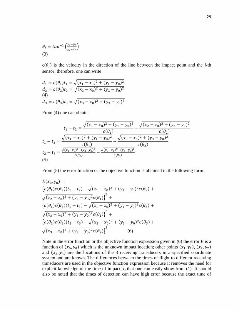
Note in the error function or the objective function expression given in (6) the error E is a

function of ( ) which is the unknown impact location; other points ( ), ( ) and ( ) are the locations of the 3 receiving transducers in a specified coordinate

system and are known. The differences between the times of flight to different receiving

transducers are used in the objective function expression because it removes the need for

explicit knowledge of the time of impact, tc that one can easily show from (1). It should

also be noted that the times of detection can have high error because the exact time of

30

detection is often hidden in the noise; taking the difference between two times of

detection can reduce this error.

In (6) all three transducers are given the same weight or importance. ( ) is the wave

speed in the direction of the line connecting ( ) and ( ), the wave speeds are

different in different directions and are obtained experimentally. Ideally, for the correct

values of ( ) the error function should give a zero value, while for incorrect values

of ( ) it should give a positive value. Because all terms in the error function are

squared, E should be a positive value or zero. Therefore, the point which gives the least

value of the error function should be closest to the exact point of impact.

There are different methods of optimization that can be used for minimizing a function.

One method that has been investigated before [1, 2] is based on introducing a mesh grid

in the plate. After evaluating the nonlinear objective function at the grid points and

finding the coordinate of the grid point where the function value is minimum the impact

point is predicted. Accuracy of this technique depends on how fine a mesh is chosen.

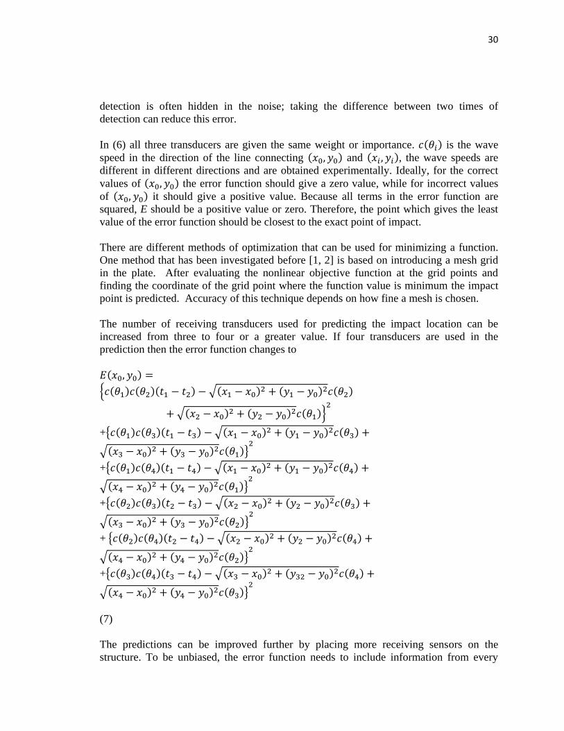
The number of receiving transducers used for predicting the impact location can be

increased from three to four or a greater value. If four transducers are used in the

prediction then the error function changes to

( )

{ ( ) ( )( ) √( ) ( )

( )

√( ) ( )

( )}

+{ ( ) ( )( ) √( ) ( )

( )

√( ) ( )

( )}

+{ ( ) ( )( ) √( ) ( )

( )

√( ) ( )

( )}

+{ ( ) ( )( ) √( ) ( )

( )

√( ) ( )

( )}

+ { ( ) ( )( ) √( ) ( )

( )

√( ) ( )

( )}

+{ ( ) ( )( ) √( ) ( )

( )

√( ) ( )

( )}

(7)

The predictions can be improved further by placing more receiving sensors on the

structure. To be unbiased, the error function needs to include information from every

31

possible sensor pair. Therefore, an increase in the number of sensors gives an increase in

the number of terms in the error function, and therefore an increase in the run time of the

code. With three sensors the number of terms in the function is three (as given in Eq. 6);

by changing the number of sensors to four, the number of terms increases to six as one

can see in (7).

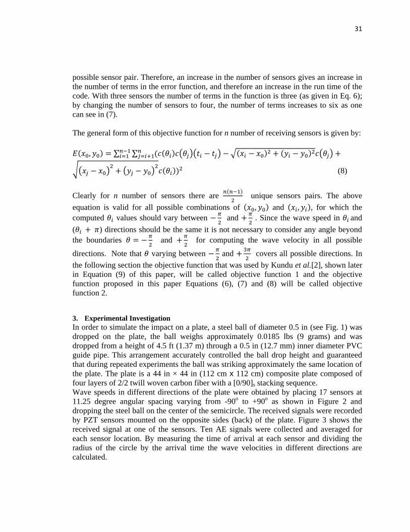
The general form of this objective function for n number of receiving sensors is given by:

( ) ∑ ∑ ( ( ) ( )( ) √( ) ( )

( )

√( ) ( )

( ))

(8)

Clearly for n number of sensors there are ( )

unique sensors pairs. The above

equation is valid for all possible combinations of ( ) and ( ), for which the

computed values should vary between

and

. Since the wave speed in and

( ) directions should be the same it is not necessary to consider any angle beyond

the boundaries

and

for computing the wave velocity in all possible

directions. Note that varying between

and

covers all possible directions. In

the following section the objective function that was used by Kundu et al.[2], shown later

in Equation (9) of this paper, will be called objective function 1 and the objective

function proposed in this paper Equations (6), (7) and (8) will be called objective

function 2.

3. Experimental Investigation

In order to simulate the impact on a plate, a steel ball of diameter 0.5 in (see Fig. 1) was

dropped on the plate, the ball weighs approximately 0.0185 lbs (9 grams) and was

dropped from a height of 4.5 ft (1.37 m) through a 0.5 in (12.7 mm) inner diameter PVC

guide pipe. This arrangement accurately controlled the ball drop height and guaranteed

that during repeated experiments the ball was striking approximately the same location of

the plate. The plate is a 44 in × 44 in (112 cm x 112 cm) composite plate composed of

four layers of 2/2 twill woven carbon fiber with a [0/90]s stacking sequence.

Wave speeds in different directions of the plate were obtained by placing 17 sensors at

11.25 degree angular spacing varying from -90o to +90

o as shown in Figure 2 and

dropping the steel ball on the center of the semicircle. The received signals were recorded

by PZT sensors mounted on the opposite sides (back) of the plate. Figure 3 shows the

received signal at one of the sensors. Ten AE signals were collected and averaged for

each sensor location. By measuring the time of arrival at each sensor and dividing the

radius of the circle by the arrival time the wave velocities in different directions are

calculated.

32

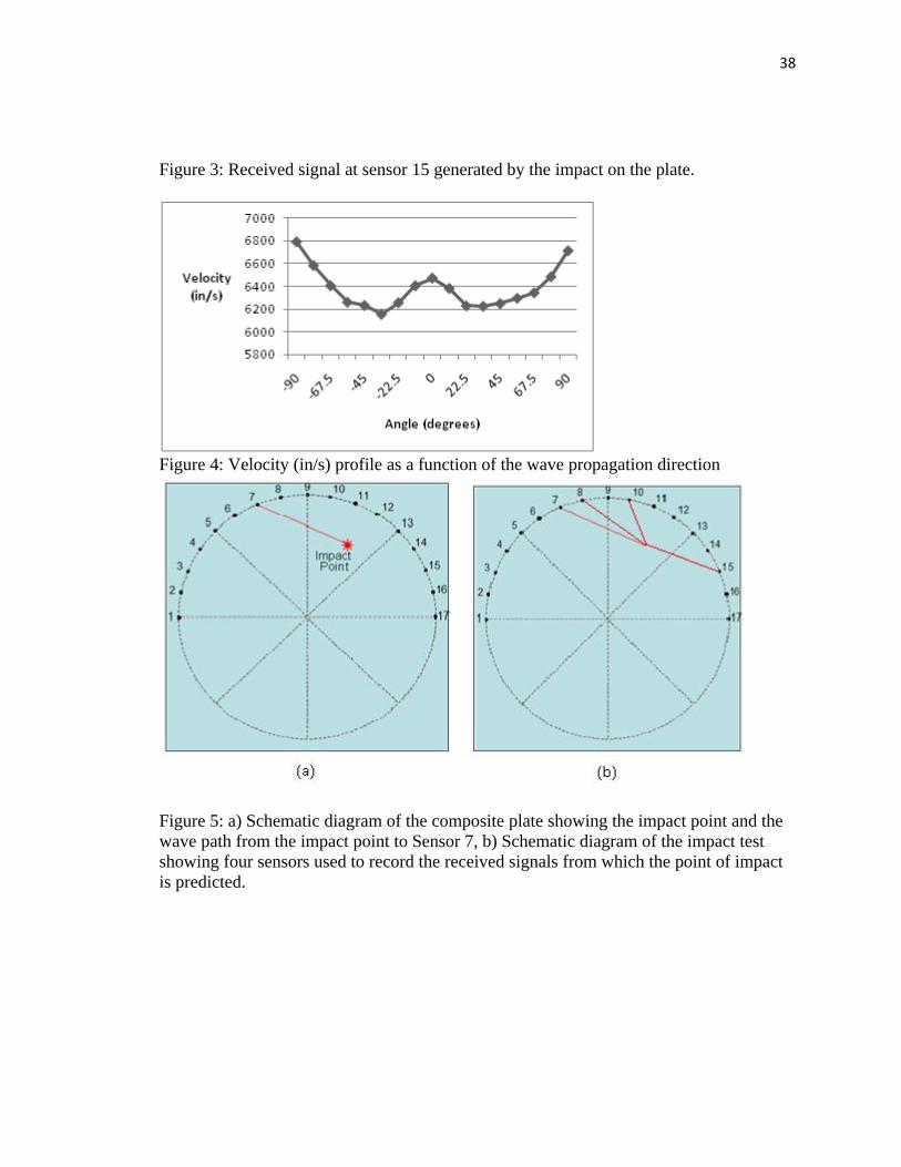
Experimentally measured guided wave speeds in the 0-90 cross ply composite plate

varying from - to + are shown in Figure 4. As expected, the wave speeds in the

fiber directions, and are relatively higher. Since the composite plate is not

perfectly symmetric the velocity profile is not symmetric about the zero degree line, the

wave speeds in the and directions are different. Wave speeds in the

and directions are the smallest. After experimentally obtaining the wave speeds

in 17 discrete angular directions, the wave speed in any angular direction [c(θ)] is

obtained by fitting a natural cubic spline through the experimental points, as shown in

Figure 4.

After obtaining the velocity profile, a second set of tests were carried out to predict the

impact location. A point was chosen randomly to be the impact point and the steel ball

was dropped on that point, four of the attached 17 transducers were chosen to be the

receiving sensors for the second set of experiments. Similar to the first set of experiments

ten signals were collected by every sensor and the average of these ten signals were used

as the receiving signal. Schematic diagram of the composite plate with mounted acoustic

emission sensors for the second set of experiments are shown in Figure 5a. In this figure

the impact point is shown by the star and the receiving sensor which collects the data is

the transducer number 7 in Figure 5a or 7, 8, 10 and 15 in Figure 5b. For every impact

test 4 sensors were chosen to collect the signals. The received signals are similar to the

signal shown in Figure 3. It is not easy to measure the exact time of arrival of the signals

from the time history plots because there is some ambiguity in these plots about the

starting point of the signals due to the presence of a low level noise in the time history

plots before the actual arrival time of the ultrasonic energy. The exact arrival time is

hidden in this noise. Therefore, the actual arrival times at different sensors are probably

smaller than the recorded times. However, since the objective function (see Equations 7

and 8) uses the difference in the recorded arrival times these small errors in the recording

should nullify one another and the final results should not be affected significantly. For

the first test the steel ball was dropped at a point whose coordinates are given by x = 29.4

in, y = 33.7 in, measured from the origin located at the bottom left corner of the plate and

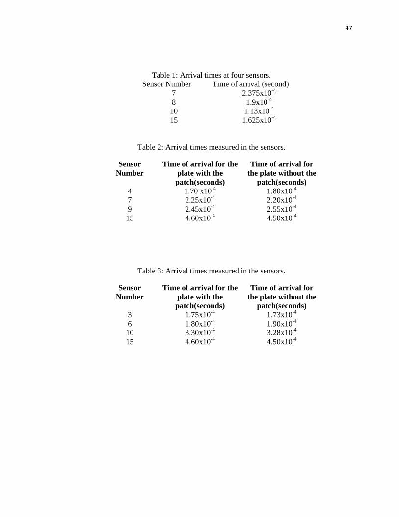
the signals were recorded by the transducers 7, 8, 10, and 15 as shown in Figure 5b.The

following times given in Table 1, were recorded as the arrival times at the four sensors.

These times and the coordinates of the transducers were used as the inputs for the

MATLAB code that minimizes the objective functions. The results are shown in Figures

6 to 11.

Objective functions 2 (given in Equation 8) and 1 (described in reference 2, and given in

Equation 9 of this paper) using three transducers are so sensitive to the small variations of

the time of flight measurement, that by changing just one of the measured times of arrival

by a small amount (say 5%), the prediction can be significantly altered. It seems that

when the objective function 1 is used with three receiving transducers and a specified

(5% or 10%) variation in the arrival time is introduced the prediction points are scattered

over a wide region of the plate. When predicted impact points from different sets of

transducers are plotted on the same figure the predicted points from all sets go through a

common region which is very close to the actual impact point as discussed in detail in the

following section.

33

3.1. Results from Four Sets of Three Transducers

For the first prediction four different sets of transducers with three receiving sensors in

every set that differs by at least one transducer from the other sets are taken and the times

of flight are slightly varied (5%, 10% etc.). The developed algorithm finds the impact

point for small variations of the times of flight by plotting the global minimum points.

These points are located in the valley of the surface plot of the objective function

variation. As different sets of the receiving sensors are considered the valleys of the

objective function surface plots change. However, different valleys show a common

region of intersection. The global minima points predicted by different sets of receiving

sensors go through this common region. This common region or point is the predicted

impact location. It is found that the proposed objective function can accurately predict the

point of impact even with 10 percent variation in the time of flight measurement when

this approach is followed.

The four sensors listed in Table 1 were the first set of sensors that were used as the

receiving sensors; Predicted impact points from these four sets of receiving transducers

are shown in Figure 6. Predictions from different sets are denoted by different symbols in

the figure. Every point plotted in this figure is the impact point predicted using the arrival

times obtained from the recorded signals after artificially introducing up to 5% error.

About 50 points are plotted for every set of three transducers. The final prediction of the

impact location is the intersection point or common point of these different sets of

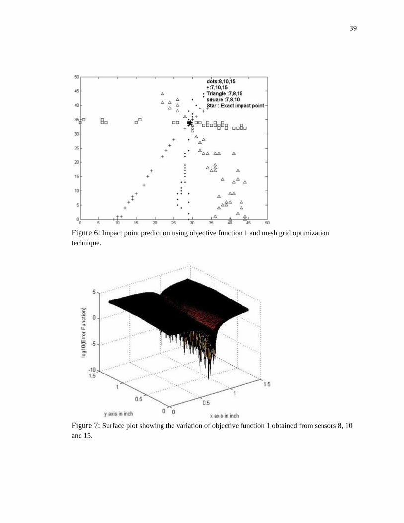
predicted points. In Figure 6 objective function 1 is used and the method of optimization

is the mesh grid technique, discussed in references 1 and 2. This technique was also used

in reference [14]. In the mesh grid technique first a rectangular mesh grid is formed on

the surface of the plate, then the objective function is calculated at the grid points. The y-

coordinates corresponding to the minimum values of the objective function for different

x-values are obtained, then among these multiple minima the absolute minimum value of

the objective function is identified; x and y values corresponding to this absolute

minimum are the coordinates of the impact point and are plotted with different symbols

for different sets of sensors. For each set of sensors 50 predictions are made for 50

different sets of arrival times having up to 5 percent error in evary set. One can see in

Figure 6 that the minimum points from a specific set of sensors are not located in a small

region but widely scattered along a line. This is because from the surface plot of the

objective function given in Figure 7 one can see that the minimum of the objective

function is not a clearly defined point but multiple minima exist along a long valley.

Figure 7 shows the surface plot of the objective function for the sensor set that includes

sensors 8, 10 and 15. When small errors (~5%) are introduced in the arrival times the

absolute minimum point moves from one point to another point in this valley.

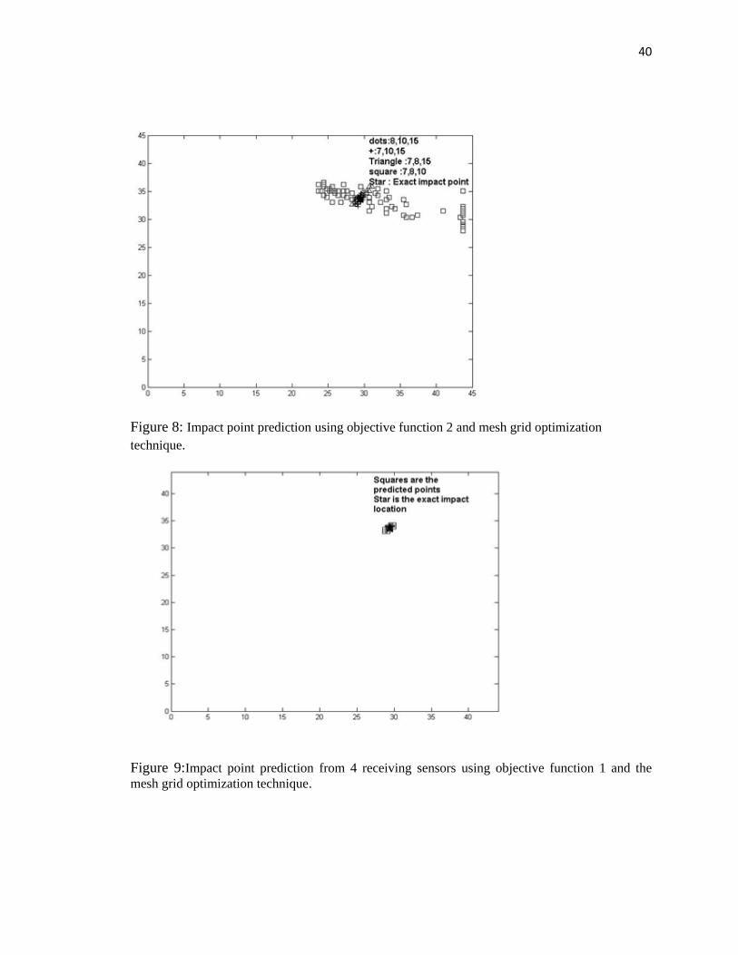
Figure 8 is obtained from the same sets of receiving sensors with 5 % variations in the

arrival time while using the objective function 2. Predicted points are now less scattered

compared to Figure 6 except for one set that is plotted by square symbols (sensors 7, 8

and 10). It can be seen in Figure 8 that all predictions from one set of sensors (8, 10 and

34

15) are very close to the actual impact point. Therefore, the objective function 2 requires

less computational time and converges faster compared to the objective function 1.

3.2. Results from Four Transducers Working Simultaneously

When the signal is recorded by four transducers the point of impact can be predicted by

substituting the four arrival times in objective function 1 [14] or objective function 2

defined in this paper. The objective function 1 for four receiving sensors is given by

( ) ∑ ∑ ∑ ∑ [ ( ) ( )( ( ) ( ))

( ) ( ) ( ( ) ( ))]

(9)

In which tij (= ti - ti) is the difference between arrival times at i-th and j-th sensors and di

is the distance of the i-th sensor from the point of impact.

√( ) ( )

(10)

Note that di is the distance between the impact point ( ) and the ith

sensor( ). Objective function 2 (Equation 7) for four transducers working together has 6 terms in

comparison to the objective function 1 (Equation 9) that has 15 terms. Thus the

calculation time is significantly reduced for objective function 2. In Figures 9 and 10

objective functions 1 and 2 are used for predicting the impact point location using the

same input data but four sensors working together. It can be seen in these figures that

these two objective functions are less sensitive to the time of flight measurement error

when arrival times at all four sensors are considered in the objective function expression.

All of the predicted impact points were found to be very close to the actual point of

impact denoted by the black star. The prediction accuracy is almost same in Figures 9 and

10; however, the objective function 2 requires less computation time.

There is another type of error that can arise during the experimental investigaton; it is the

velocity profile measurement error. It is then investigated if the velocity profile

measurement error has the same effect as the time of the flight recording error. For this

investigation the recorded velocity profile, Figure 4, was artificially altered to introduce

up to 5 percent error. Predictions of the impact point using the altered velocity profile are

shown in Figures 11 and 12. Figure 11 is generated by giving uniform (5%) error in the

velocity measurement in all directions while Figure 12 is generated by giving random

(within 5%) error in different directions.

4. Results for Non-Homogeneous Plate:

The next set of tests were carried out with the same plate after attaching a patch to the

plate in order to determine how the prediction is affected by the plate inhomogenity. Two

sizes of doubler patches were used as the interfering objects on the wave propagation

paths. The doubler patches were made from the original plate material.

35

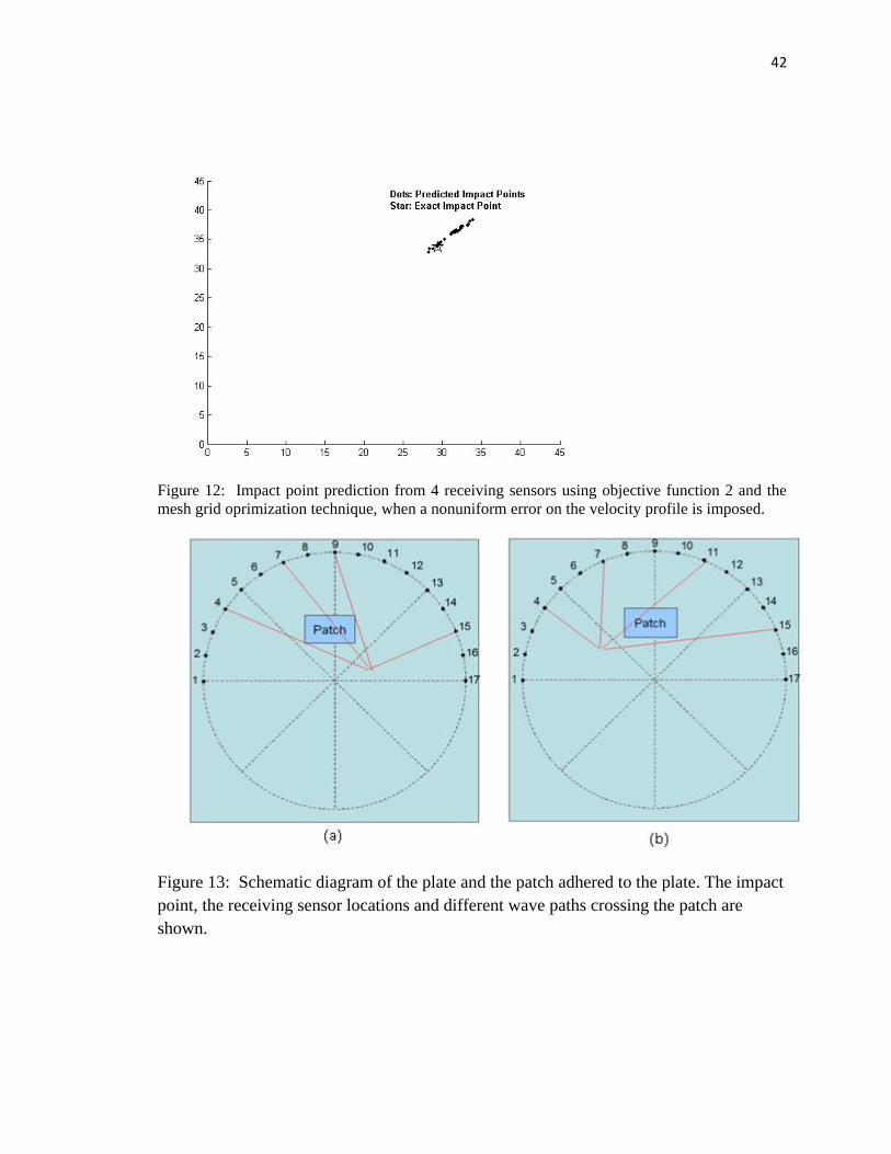
The first specimen was fabricated by attaching a small doubler patch (4 in.× 8 in or 10.16

cm x 20.32 cm) to the plate. Figure 13 shows the schematic diagram of the plate with the

patch and the receiving sensor locations. The lines show the signal propagation paths

from the impact point to the receiving sensors.

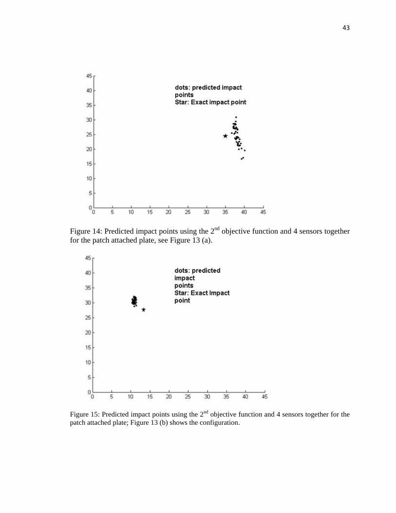
In order to determine the difference in response, the plates were impacted by the ball at

the same location with and without the doubler patch.. The same algorithm was used to

predict the impact location using the times of arrival got from the signals . The predicted

results are shown in Figure 14; objective function 2 using 4 sensors simultaneously was

used to predict these impact point locations. Different impact points are obtained by

introducing a random 5 percent variation in the arrival times.

For the other configuration shown in Figure 13(b), the impact point was changed and the

point of impact was predicted using the time of arrivals at sensors 4, 7, 11 and 15. Figures

15 and 16 show the predicted impact points using 4 sensors simultaneously and objective

function 2. Comparing Figures 15 and 16 one can say that although the attached doubler

patch reduces the accuracy of the impact point prediction, the overall impact location

performance is not significantly degraded.

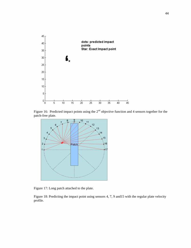
The second doubler patch is a long strip (30 in × 4 in) as shown in Figure 17. In this case,

the doubler patch crosses more than half of the impact site to sensor paths. This test

configuration approximates the effect of the plate stiffener.

Table 2 indicates the time of arrival from the signals when there was no patch attached to

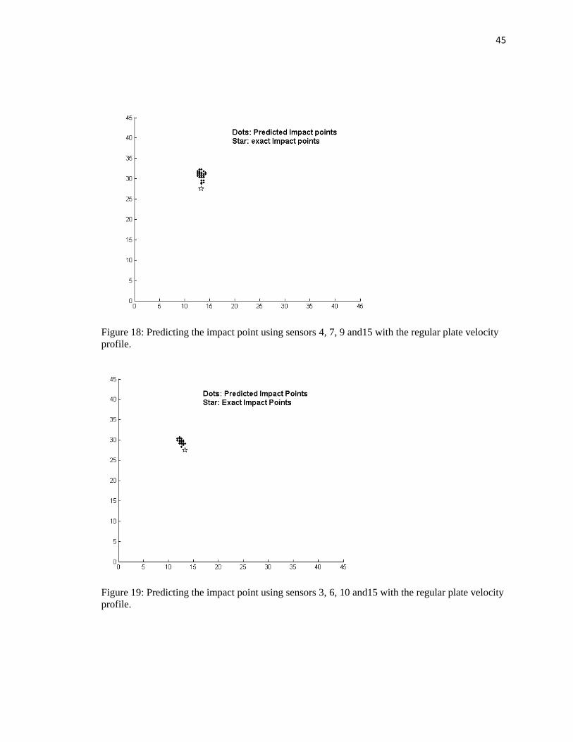
the plate and when the long strip was attached to the plate. Figures 18 and19 show the

predicted results from two different sets of sensors obtained using the second objective

function. In both cases the predicted impact points are found to be slightly on the left of

the true point of impact. This occurs because the wave speed data does not include the

doubler patch. The doubler patch affects the velocity profile but that change was not

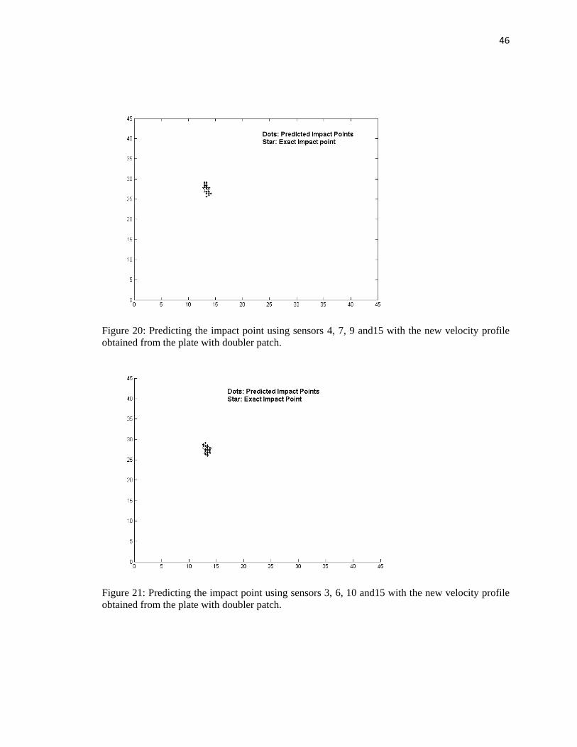
considered in the analysis. If a new velocity profile is generated in presence of the patch

and that profile is used to predict the impact point then the prediction accuracy improves

as shown in Figures 20 and 21.

5. Conclusion

A new algorithm for accurately predicting the impact point on an anisotropic plate is

introduced and verified experimentally. The objective function proposed by Kundu et al.

[1,2] is modified to make it computationally more efficient. Using the modified objective

function and four sensors instead of three the prediction accuracy is significantly

improved. The algorithm has been tested on homogeneous as well as non-homogeneous

plates. Non-homogeneous plates were fabricated by stiffening the plate at selected

segments. Stiffening was achieved by applying a doubler patch at desired locations.

36

ACKNOWLEDGEMENT

This material is based upon the work supported by the Air Force Office of Scientific

Research (AFOSR) under Contract No. FA9550-09-C-0122. Opinions, findings,

conclusions and recommendations given in this paper are those of the authors and do not

necessarily reflect the views of AFOSR.

REFERENCES

1- T. Kundu, S. Das and K. V. Jata, “Point of Impact Prediction in Isotropic and Anisotropic

Plates from the Acoustic Emission Data”, Journal of the Acoustical Society of America,

Vol. 122 (4), pp. 2057-2066, 2007

2- T. Kundu, S. Das, S. A. Martin and K. V. Jata, “Locating point of impact in anisotropic

fiber reinforced composite plates”, Ultrasonics, Vol 48, Issue 3, pp 193-201, July 2008

3- K. V. Jata, T. Kundu, and T. Parthasarathy, “An introduction to failure mechanisms and ultrasonic inspection,” in Advanced Ultrasonic Methods for Material and Structure Inspection, edited by T. Kundu _ISTE, London, 2007_, Chap. 1, pp. 1–42.

4- V. Giurgiutiu, “Lamb wave generation with piezoelectric wafer active sensors for structural health monitoring,” Proc. SPIE 5056, 111–122 _2003_.

5- A. K. Mal, F. Shih and S. Banerjee, Acoustic Emission Waveforms in Composite

Laminates under Low Velocity Impact, Proceedings of SPIE 5047 (2003) 1-12.

6- A. K. Mal, F. Ricci, S. Gibson and S. Banerjee, Damage Detection in Structures from

Vibration and Wave Propagation Data, Proceedings of SPIE 5047 (2003) 202-210.

7- B. Köhler, F. Schubert and B. Frankenstein, Numerical and Experimental Investigation

of Lamb Wave Excitation, Propagation and Detection for SHM, Proceedings of the

second European Workshop on Structural Health Monitoring (2004) 993-1000.15

8- J. Park and F. K. Chang, Built-In Detection of Impact Damage in Multi-Layered Thick

Composite Structures, Proceedings of the fourth International Workshop on Structural

Health Monitoring (2003) 1391-1398.

9- A. K. Mal, F. Ricci, S. Banerjee and F. Shih, A Conceptual Structural Health Monitoring

System Based on Wave Propagation and Modal Data, Str. Health Monit. : Int. J. 4 (2005)

283-293.

10- G. Manson, K. Worden, K. and D. J. Allman, Experimental Validation of Structural

Health Monitoring Methodology II: Novelty Detection on an Aircraft Wing, J. Sound

Vib. 259 (2003) 345-363.

11- S. C. Wang and F. –K Chang, Diagnosis of Impact Damage in Composite Structures

with Built-in Piezoelectrics Network, Proceedings of SPIE 3990 (2000) 13-19.

12- S. S. Kessler, S. M. Spearing, and C. Soutis, Damage Detection in Composite Materials

using Lamb Wave Methods, Smt. Mater. Str. 12 (2002) 795-803.

13- T. Kundu, S. Das and K. V. Jata, An Improved Technique for Locating the Point of

Impact from the Acoustic Emission Data, Proceedings of SPIE 6532 (2007).

14- T. Kundu, S. Das and K. V. Jata, Point of Impact Prediction in Anisotropic Fiber

Reinforced Composite Plates from the Acoustic Emission Data, Review of Progress in

Quantitative Nondestructive Evaluation, Am. Inst. of Physics (2007).

15- W. Sachse and S. Sancar, Acoustic Emission Source Location on Plate-Like Structures

Using a Small Array of Transducers, U.S. Patent No. 4,592,034 (1986).

37

16- B. Castagnede, W. Sachse, and K. Y. Kim, Location of Pointlike Acoustic Emission

Sources in Anisotropic Plates, J. Acoust. Soc. Am. 86 (1989) 1161-1171.

17- J. A. Nelder and R. Mead, A Simplex Method for Function Minimization, Comp. J. 7

(1965) 308-315.

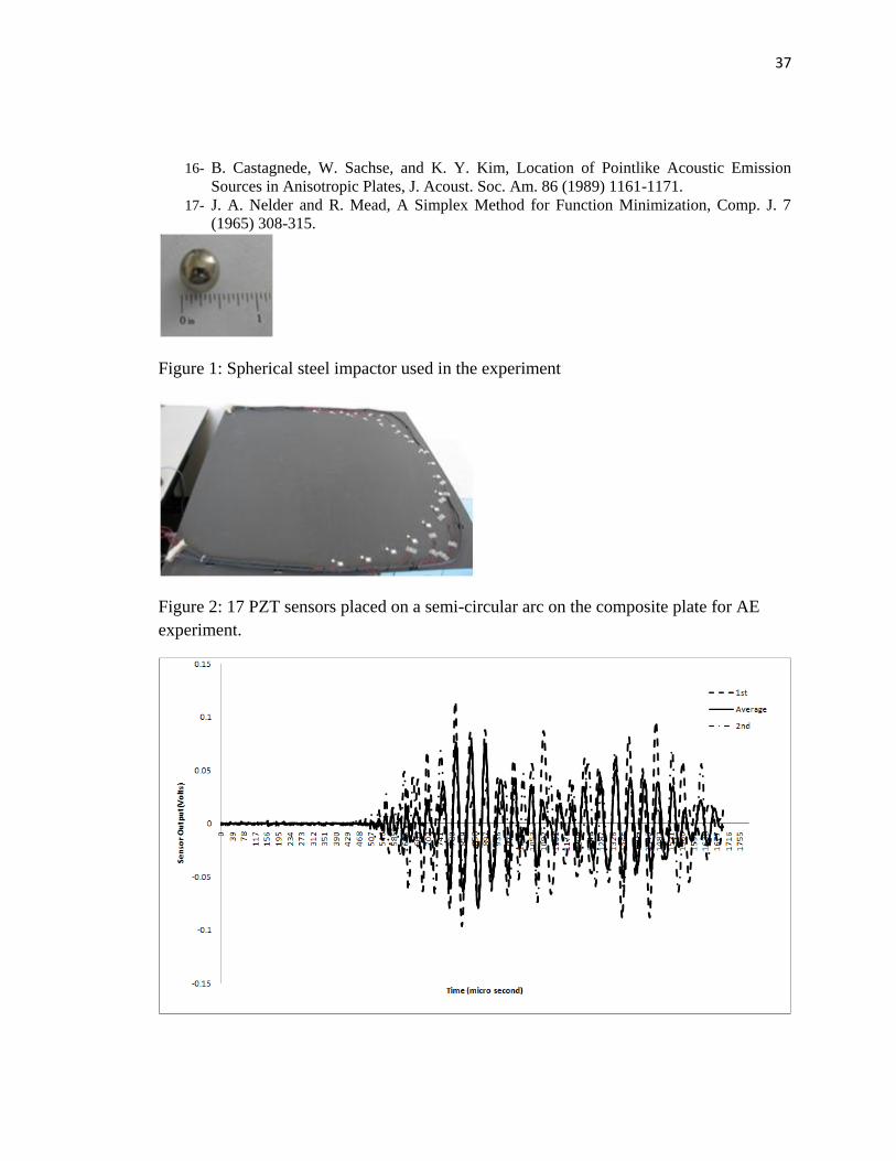
Figure 1: Spherical steel impactor used in the experiment

Figure 2: 17 PZT sensors placed on a semi-circular arc on the composite plate for AE

experiment.

38

Figure 3: Received signal at sensor 15 generated by the impact on the plate.

Figure 4: Velocity (in/s) profile as a function of the wave propagation direction

Figure 5: a) Schematic diagram of the composite plate showing the impact point and the

wave path from the impact point to Sensor 7, b) Schematic diagram of the impact test

showing four sensors used to record the received signals from which the point of impact

is predicted.

39

Figure 6: Impact point prediction using objective function 1 and mesh grid optimization

technique.

Figure 7: Surface plot showing the variation of objective function 1 obtained from sensors 8, 10

and 15.

40

Figure 8: Impact point prediction using objective function 2 and mesh grid optimization

technique.

Figure 9:Impact point prediction from 4 receiving sensors using objective function 1 and the

mesh grid optimization technique.

41

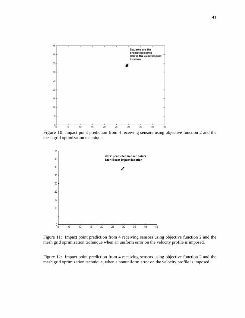
Figure 10: Impact point prediction from 4 receiving sensors using objective function 2 and the

mesh grid optimization technique

Figure 11: Impact point prediction from 4 receiving sensors using objective function 2 and the

mesh grid oprimization technique when an uniform error on the velocity profile is imposed.

Figure 12: Impact point prediction from 4 receiving sensors using objective function 2 and the

mesh grid oprimization technique, when a nonuniform error on the velocity profile is imposed.

42

Figure 12: Impact point prediction from 4 receiving sensors using objective function 2 and the

mesh grid oprimization technique, when a nonuniform error on the velocity profile is imposed.

Figure 13: Schematic diagram of the plate and the patch adhered to the plate. The impact

point, the receiving sensor locations and different wave paths crossing the patch are

shown.

43

Figure 14: Predicted impact points using the 2nd

objective function and 4 sensors together

for the patch attached plate, see Figure 13 (a).

Figure 15: Predicted impact points using the 2nd objective function and 4 sensors together for the

patch attached plate; Figure 13 (b) shows the configuration.

44

Figure 16: Predicted impact points using the 2nd objective function and 4 sensors together for the

patch-free plate.

Figure 17: Long patch attached to the plate.

Figure 18: Predicting the impact point using sensors 4, 7, 9 and15 with the regular plate velocity

profile.

45

Figure 18: Predicting the impact point using sensors 4, 7, 9 and15 with the regular plate velocity

profile.

Figure 19: Predicting the impact point using sensors 3, 6, 10 and15 with the regular plate velocity

profile.

46

Figure 20: Predicting the impact point using sensors 4, 7, 9 and15 with the new velocity profile

obtained from the plate with doubler patch.

Figure 21: Predicting the impact point using sensors 3, 6, 10 and15 with the new velocity profile

obtained from the plate with doubler patch.

47

Table 1: Arrival times at four sensors.

Sensor Number Time of arrival (second)

7 2.375x10-4

8 1.9x10-4

10 1.13x10-4

15 1.625x10-4

Table 2: Arrival times measured in the sensors.

Sensor

Number

Time of arrival for the

plate with the

patch(seconds)

Time of arrival for

the plate without the

patch(seconds)

4 1.70 x10-4

1.80x10-4

7 2.25x10-4

2.20x10-4

9 2.45x10-4

2.55x10-4

15 4.60x10-4

4.50x10-4

Table 3: Arrival times measured in the sensors.

Sensor

Number

Time of arrival for the

plate with the

patch(seconds)

Time of arrival for

the plate without the

patch(seconds)

3 1.75x10-4

1.73x10-4

6 1.80x10-4

1.90x10-4

10 3.30x10-4

3.28x10-4

15 4.60x10-4

4.50x10-4

48

APPENDIX B

DETECTING THE POINT OF IMPACT ON A CYLINDRICAL

PLATE BY THE ACOUSTIC EMISSION TECHNIQUE

This work has been published in the SPIE proceedings:

T. Hajzargarbashi, H. Nakatani, T. Kundu and N. Takeda, “Detecting the

Point of Impact on a Cylindrical Plate by the Acoustic Emission

Technique”,Proceedings of SPIE 7981, 79810U, (2011).

49

Detecting the Point of Impact on a Cylindrical Plate by the

Acoustic Emission Technique

Talieh Hajzargarbashi1, Hayato Nakatani2, Tribikram Kundu1 and Nobuo Takeda2

1Department of Civil Engineering & Engineering Mechanics, University of Arizona, Tucson, AZ 85721,

USA

2Department of Frontier Science, University of Tokyo, Kashiwnoha, Chiba, Japan

Abstract:

An optimization based technique for detecting the impact point on isotropic and anisotropic flat plates

developed by Kundu and his associates [1-3] is extended here to the cylindrical geometry. An objective

function is defined that uses the cylindrical coordinates of four sensors attached to the cylinder and four

arrival times to locate the point of impact by minimizing the objective function that gives the least squares

error. The proposed technique is experimentally verified by predicting the points of impact and comparing

the predicted points with the actual points of impact.

Key Words: Lamb Wave, Impact, Acoustic Emission, Passive Monitoring, Cylindrical Surface,

Optimization.

1. Introduction Detecting the point of impact on an anisotropic plate is of interest for finding and fixing the delaminations

or any other types of defects arising from an impact. The first step is locating the impact point where the

plate has been hit. A popular method for detecting the point of impact is the acoustic emission technique.

This technique has been used on isotropic plates. Using passive sensors attached to the isotropic plate the

point of impact can be detected by the acoustic emission method following the triangulation technique

[4,5]. For efficiently monitoring the plate the sensors need to be placed near the critical locations of the

plate [6-11]. In anisotropic plates the wave speed is not the same in all directions and therefore the

triangular technique does not work [1, 12, 13], Kundu et al. [1] proposed an alternative method which is

based on minimizing a nonlinear error function to find the specific point which satisfies all equations. The

original objective function was modified by Kundu et al. [14] to be able to overcome the singularity

problems. It was then improved further [2, 3] to make the objective function simpler, shorter, more

accurate and less sensitive to errors in the time of flight measuremt. The number of sensors was increased

to get the more accurate result [2, 3, 14]. All these works reported on the acoustic emission technique have

been for detecting the point of impact on a flat plate. Cylindrical structures have many applications in

industry. Most of the fuel cylinders have cylindrical structures, Main bodies of space shuttles and air plane

fuselages have cylindrical shapes.

In 1978 Asty [15] used the triangulation technique to detect the point of impact on a spherical surface, then

in 1993 Barat et al. [16] detected the point of impact on a cylindrical surface using the triangulation

technique; none of these techniques have been experimentally verified. As it has been mentioned before the

triangulation technique does not work for an anisotropic cylinder for which the wave speed is a function of

the wave propagation direction.

50

In this paper an algorithm is introduced in which the cylindrical coordinates of the sensors attached to the

cylindrical body and the times of flight to the sensors are used to detect the point of impact. The direction

dependent velocity profile in the cylinder wall is experimentally obtained from the sensors attached to the

cylinder. The objective function which uses the cylindrical coordinates is introduced and verified

experimentally.

2. Formulation

Let the time of detection of the acoustic signal at the i-th station be . If the time of impact be then the

travel time for the signal from the impact point to the station location is

(1)

Note that in (1) both and are defined in the same time of reference.

Cylindrical coordinates of the receiving sensors S1, S2, S3 and S4 are (r, θ1, z1), (r, θ2, z2), (r, θ3, z3) and (r,

θ4, z4), respectively and the impact point coordinate is (r, θ0, z0) in which r is the radius of the cylinder. The

sensors can be attached on the outer or inner surface of the cylinder. The impact point can be also on the

outer or inner surface.

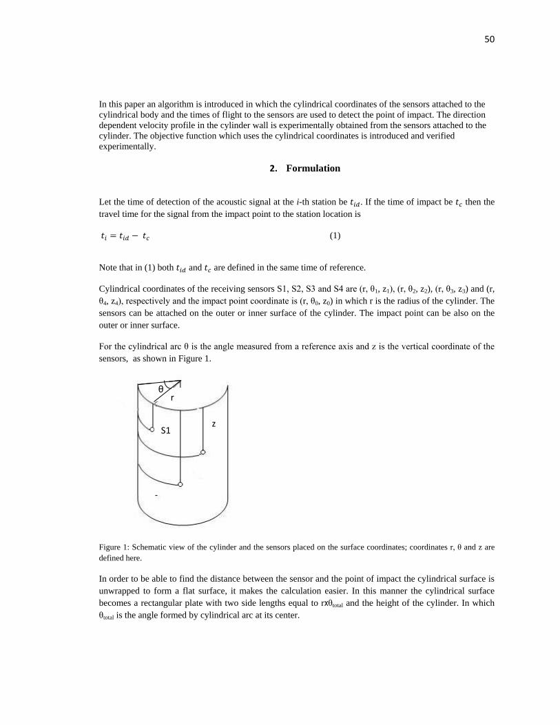
For the cylindrical arc θ is the angle measured from a reference axis and z is the vertical coordinate of the

sensors, as shown in Figure 1.

Figure 1: Schematic view of the cylinder and the sensors placed on the surface coordinates; coordinates r, θ and z are

defined here.

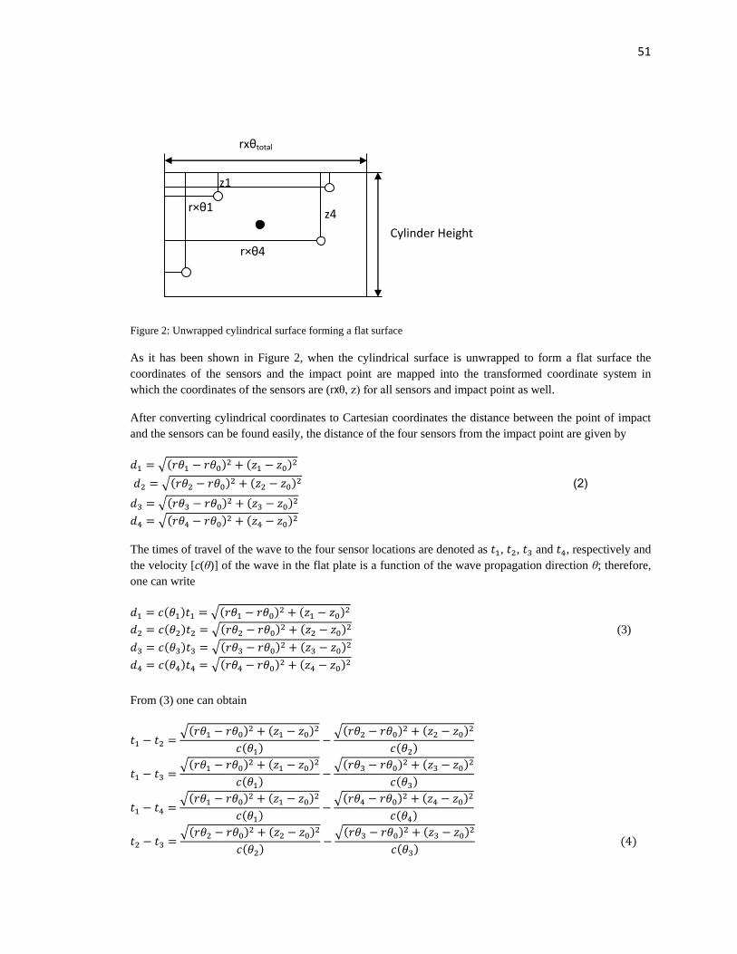
In order to be able to find the distance between the sensor and the point of impact the cylindrical surface is

unwrapped to form a flat surface, it makes the calculation easier. In this manner the cylindrical surface

becomes a rectangular plate with two side lengths equal to rxθtotal and the height of the cylinder. In which

θtotal is the angle formed by cylindrical arc at its center.

r

z

θ

S1

51

Figure 2: Unwrapped cylindrical surface forming a flat surface

As it has been shown in Figure 2, when the cylindrical surface is unwrapped to form a flat surface the

coordinates of the sensors and the impact point are mapped into the transformed coordinate system in

which the coordinates of the sensors are (rxθ, z) for all sensors and impact point as well.

After converting cylindrical coordinates to Cartesian coordinates the distance between the point of impact

and the sensors can be found easily, the distance of the four sensors from the impact point are given by

√( ) ( )

√( ) ( )

(2)

√( ) ( )

√( ) ( )

The times of travel of the wave to the four sensor locations are denoted as , , and , respectively and

the velocity [c(θ)] of the wave in the flat plate is a function of the wave propagation direction θ; therefore,

one can write

( ) √( ) ( )

( ) √( ) ( )

(3)

( ) √( ) ( )

( ) √( ) ( )

From (3) one can obtain

√( )

( )

( ) √( )

( )

( )

√( )

( )

( ) √( )

( )

( )

√( )

( )

( ) √( )

( )

( )

√( )

( )

( ) √( )

( )

( ) ( )

rxθtotal

Cylinder Height

r×θ1

z1

r×θ4

z4

52

√( )

( )

( ) √( )

( )

( )

√( )

( )

( ) √( )

( )

( )

The error function or the objective function with four arrival times (at four sensors S1, S2, S3 and S4) can

be written as:

( ) ( ) ( )( ) √( ) ( )

( )

√( ) ( )

( ) ( ) ( )( )

√( ) ( )

( ) √( ) ( )

( )

( ) ( )( ) √( ) ( )

( )

√( ) ( )

( ) ( ) ( )( )

√( ) ( )

( ) √( ) ( )

( )

( ) ( )( ) √( ) ( )

( )

√( ) ( )

( ) ( ) ( )( )

√( ) ( )

( ) √( ) ( )

( ) (5)

As it can be seen in the error function or the objective function (5) the error is a function of ( ) which

is the impact location and it is unknown, the other points which are( ) , ( ) , ( ) and ( ) are the locations of the four sensors in a specified coordination system which are known, the time of

arrivals can be recorded from the signals received by the receivers.

( ) is the wave speed in the direction of the line joining ( ) and ( ), the wave speed is

different in different directions and is obtained experimentally. Ideally, for the correct values of ( ) the error function should give a zero value, while for wrong values of ( ) it should give a positive

value so by minimizing the error function the point of impact ( ) is found.

There are different methods of optimization that can be used for minimizing this function; one method

generates mesh grid on the plate and finds the grid point corresponding to the minimum value of the

nonlinear objective function. This grid point gives the location of the impact point. Alternately, other

optimization schemes such as simplex algorithm or genetic algorithm can be also used.

The number of sensors can be increased for improving the accuracy of prediction. For n number of sensors

there are ( )

unique sensor pairs. To be unbiased, the error function needs to include information from

every unique sensor pair so by increasing the number of sensors the number of terms in the error function

or the objective function will increase and the run time of the code will also increase. With 3 sensors the

number of terms in the function is 3, by changing the number of sensors to 4 the number of terms increase

to 6.

Note that the angle of the wave propagation direction from the source ( ) to the station( ), is

measured from the horizontal axis and can be obtained from the following equation

(

) (6)

The above equation is valid for all possible combinations of ( ) and ( ) for which the Computed

values should vary between ⁄ and + ⁄ . Since the wave velocity in and ( ) directions

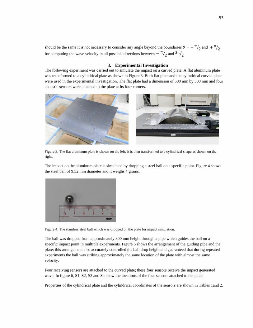
53

should be the same it is not necessary to consider any angle beyond the boundaries ⁄ and ⁄

for computing the wave velocity in all possible directions between ⁄ and ⁄

3. Experimental Investigation

The following experiment was carried out to simulate the impact on a curved plate. A flat aluminum plate

was transformed to a cylindrical plate as shown in Figure 3. Both flat plate and the cylindrical curved plate

were used in the experimental investigation. The flat plate had a dimension of 500 mm by 500 mm and four

acoustic sensors were attached to the plate at its four corners.

Figure 3: The flat aluminum plate is shown on the left; it is then transformed to a cylindrical shape as shown on the

right.

The impact on the aluminum plate is simulated by dropping a steel ball on a specific point. Figure 4 shows

the steel ball of 9.52 mm diameter and it weighs 4 grams.

Figure 4: The stainless steel ball which was dropped on the plate for impact simulation.

The ball was dropped from approximately 800 mm height through a pipe which guides the ball on a

specific impact point in multiple experiments. Figure 5 shows the arrangement of the guiding pipe and the

plate; this arrangement also accurately controlled the ball drop height and guaranteed that during repeated

experiments the ball was striking approximately the same location of the plate with almost the same

velocity.

Four receiving sensors are attached to the curved plate; these four sensors receive the impact generated

wave. In figure 6, S1, S2, S3 and S4 show the locations of the four sensors attached to the plate.

Properties of the cylindrical plate and the cylindrical coordinates of the sensors are shown in Tables 1and 2.

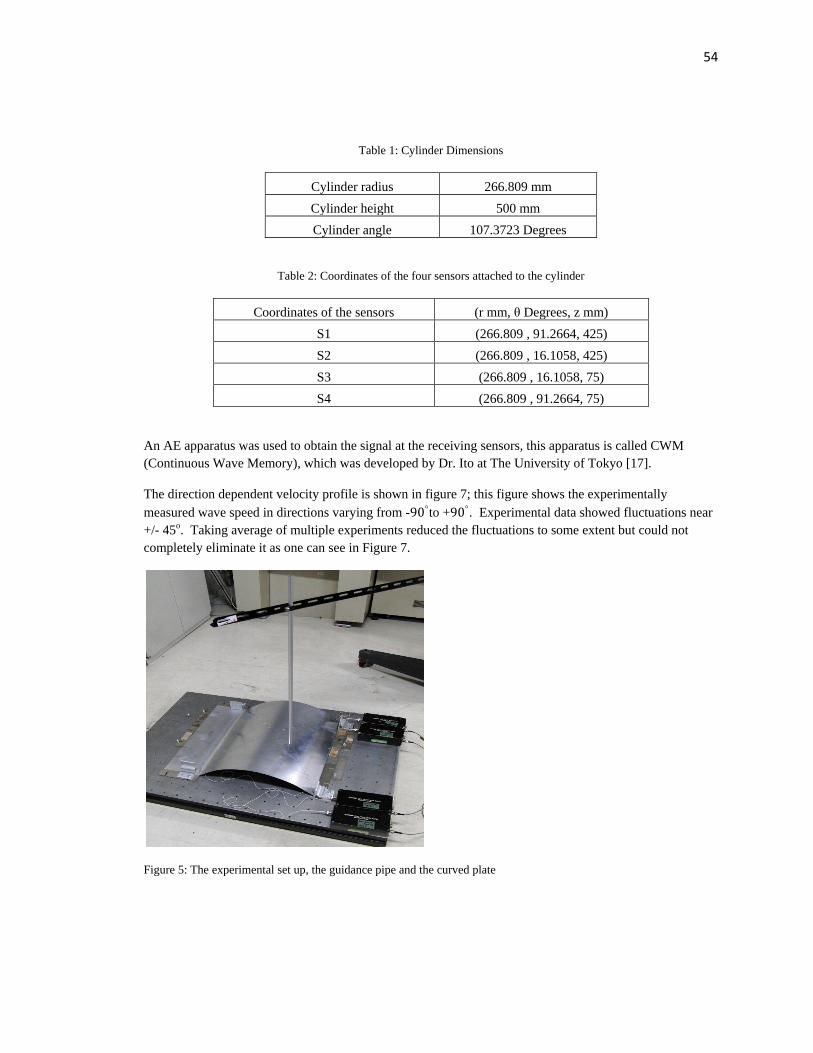
54

Table 1: Cylinder Dimensions

Cylinder radius 266.809 mm

Cylinder height 500 mm

Cylinder angle 107.3723 Degrees

Table 2: Coordinates of the four sensors attached to the cylinder

Coordinates of the sensors (r mm, θ Degrees, z mm)

S1 (266.809 , 91.2664, 425)

S2 (266.809 , 16.1058, 425)

S3 (266.809 , 16.1058, 75)

S4 (266.809 , 91.2664, 75)

An AE apparatus was used to obtain the signal at the receiving sensors, this apparatus is called CWM

(Continuous Wave Memory), which was developed by Dr. Ito at The University of Tokyo [17].

The direction dependent velocity profile is shown in figure 7; this figure shows the experimentally

measured wave speed in directions varying from - to + . Experimental data showed fluctuations near

+/- 45o. Taking average of multiple experiments reduced the fluctuations to some extent but could not

completely eliminate it as one can see in Figure 7.

Figure 5: The experimental set up, the guidance pipe and the curved plate

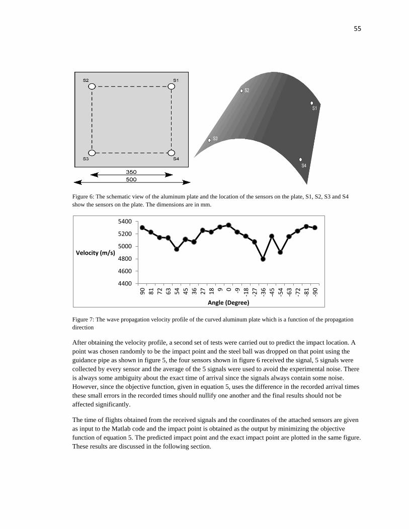
55

Figure 6: The schematic view of the aluminum plate and the location of the sensors on the plate, S1, S2, S3 and S4

show the sensors on the plate. The dimensions are in mm.

Figure 7: The wave propagation velocity profile of the curved aluminum plate which is a function of the propagation

direction

After obtaining the velocity profile, a second set of tests were carried out to predict the impact location. A

point was chosen randomly to be the impact point and the steel ball was dropped on that point using the

guidance pipe as shown in figure 5, the four sensors shown in figure 6 received the signal, 5 signals were

collected by every sensor and the average of the 5 signals were used to avoid the experimental noise. There

is always some ambiguity about the exact time of arrival since the signals always contain some noise.

However, since the objective function, given in equation 5, uses the difference in the recorded arrival times

these small errors in the recorded times should nullify one another and the final results should not be

affected significantly.

The time of flights obtained from the received signals and the coordinates of the attached sensors are given

as input to the Matlab code and the impact point is obtained as the output by minimizing the objective

function of equation 5. The predicted impact point and the exact impact point are plotted in the same figure.

These results are discussed in the following section.

4400

4600

4800

5000

5200

5400

90

81

72

63

54

45

36

27

18 9 0 -9

-18

-27

-36

-45

-54

-63

-72

-81

-90

Velocity (m/s)

Angle (Degree)

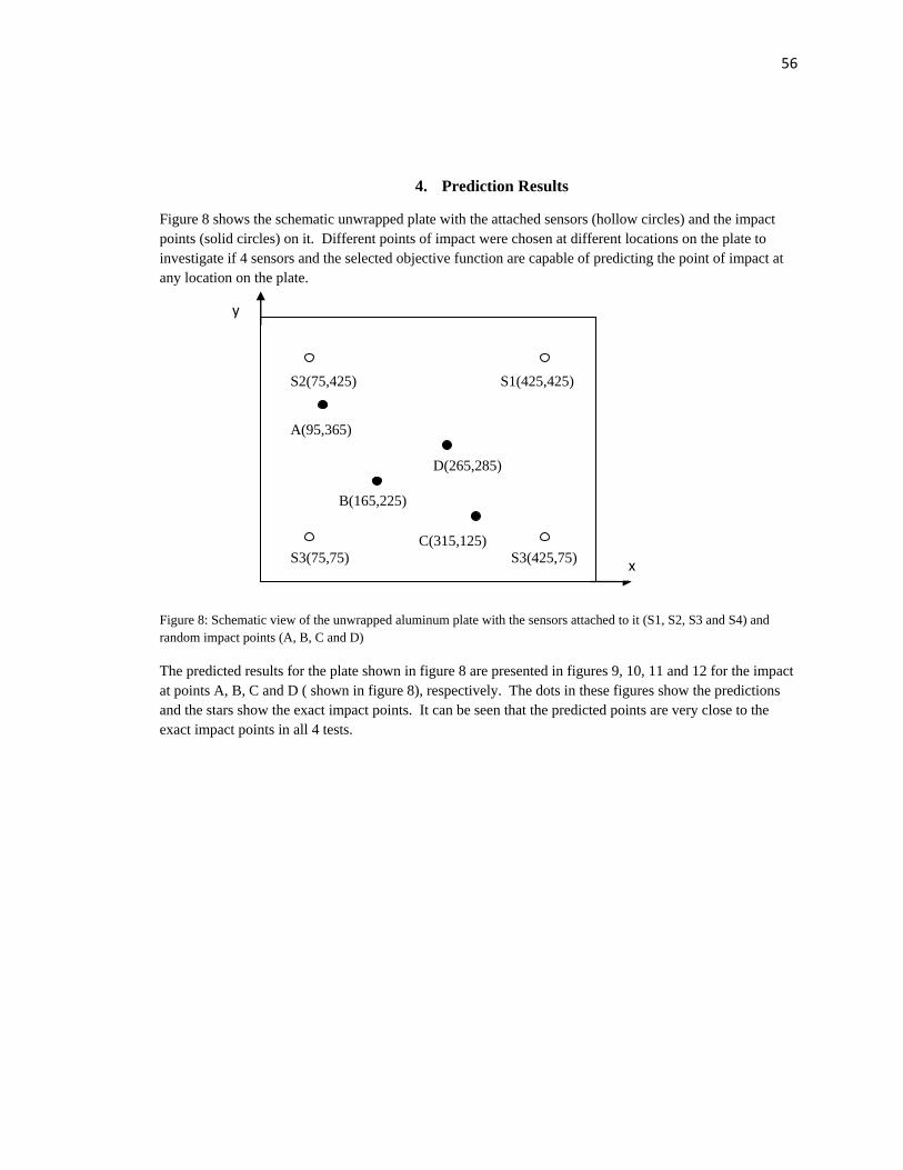
56

4. Prediction Results

Figure 8 shows the schematic unwrapped plate with the attached sensors (hollow circles) and the impact

points (solid circles) on it. Different points of impact were chosen at different locations on the plate to

investigate if 4 sensors and the selected objective function are capable of predicting the point of impact at

any location on the plate.

Figure 8: Schematic view of the unwrapped aluminum plate with the sensors attached to it (S1, S2, S3 and S4) and

random impact points (A, B, C and D)

The predicted results for the plate shown in figure 8 are presented in figures 9, 10, 11 and 12 for the impact

at points A, B, C and D ( shown in figure 8), respectively. The dots in these figures show the predictions

and the stars show the exact impact points. It can be seen that the predicted points are very close to the

exact impact points in all 4 tests.

S3(425,75)

S2(75,425) S1(425,425)

S3(75,75)

A(95,365)

B(165,225)

C(315,125)

D(265,285)

x

y

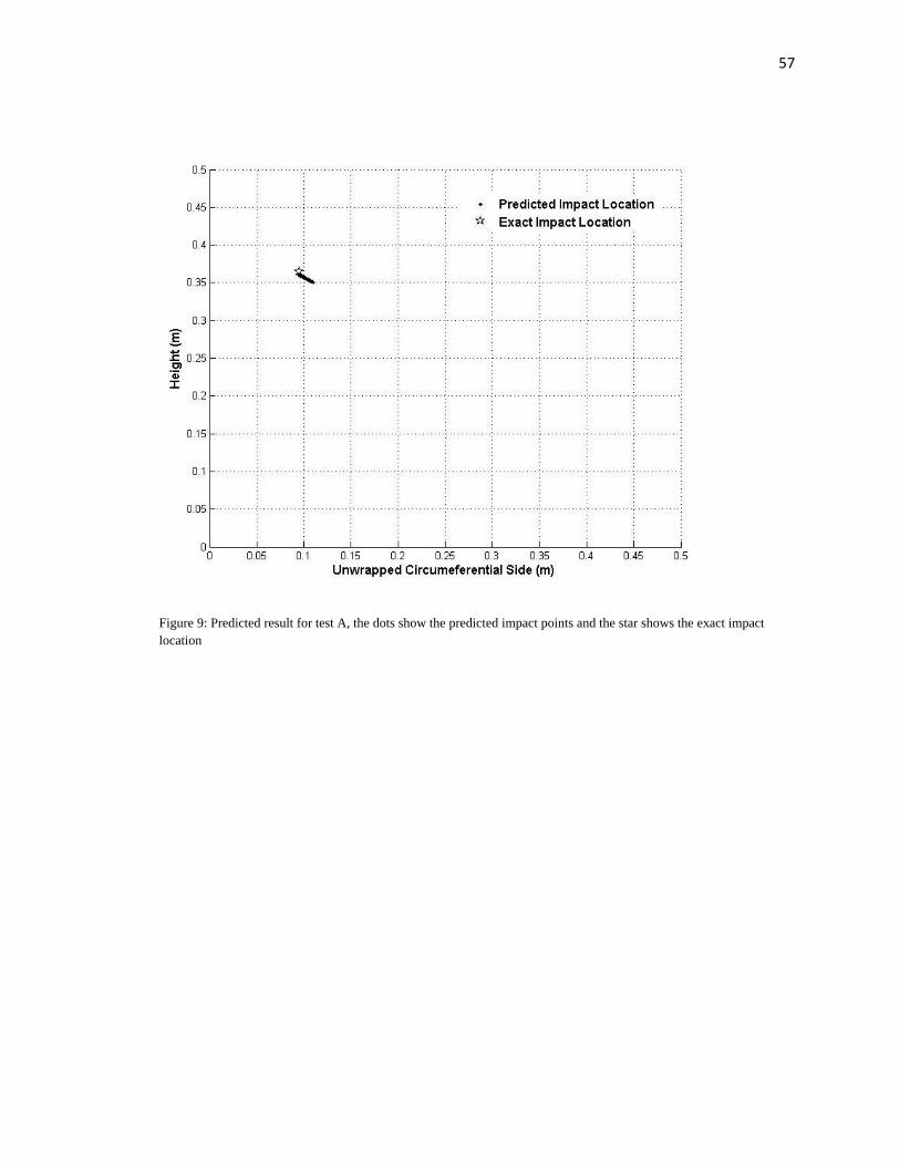
57

Figure 9: Predicted result for test A, the dots show the predicted impact points and the star shows the exact impact

location

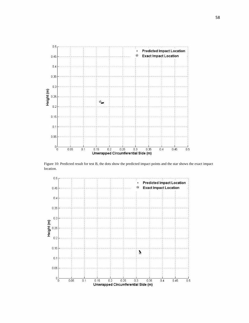
58

Figure 10: Predicted result for test B, the dots show the predicted impact points and the star shows the exact impact

location.

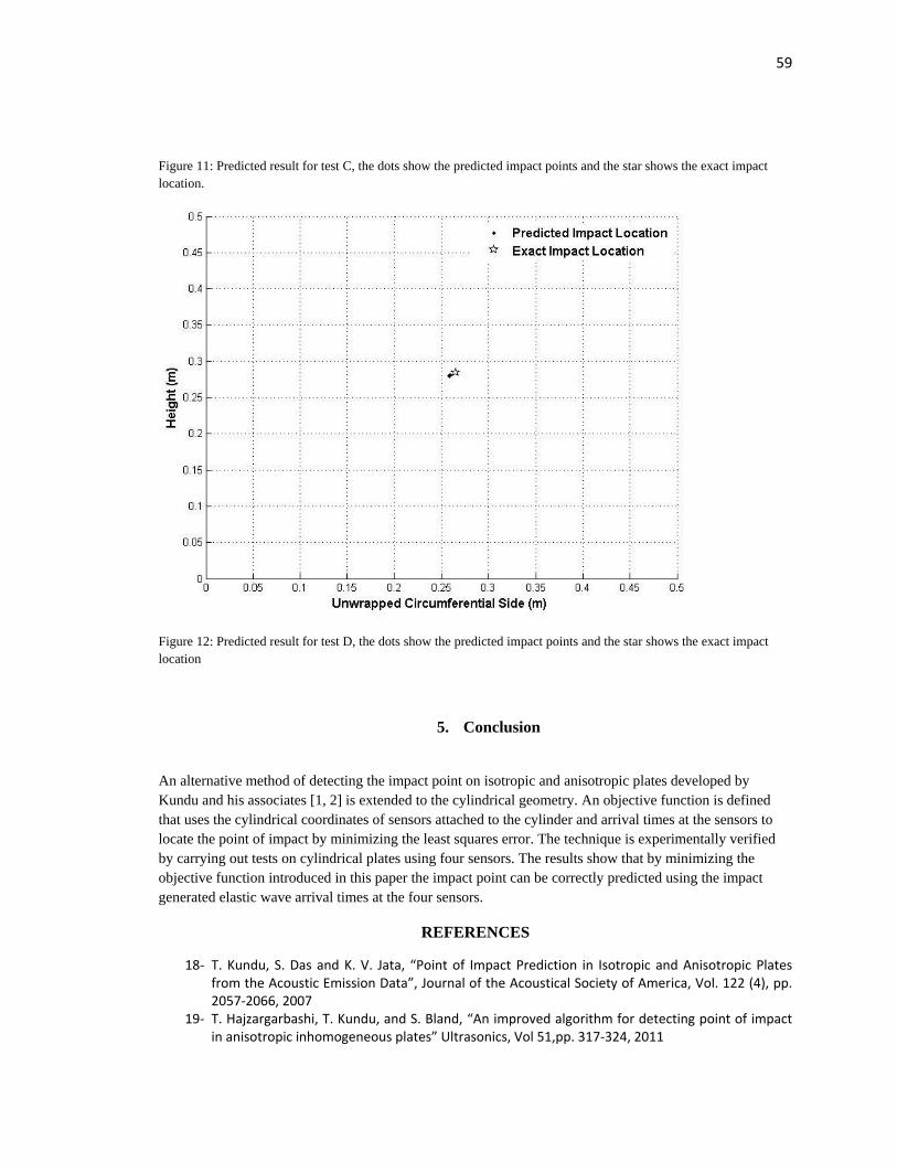
59

Figure 11: Predicted result for test C, the dots show the predicted impact points and the star shows the exact impact

location.

Figure 12: Predicted result for test D, the dots show the predicted impact points and the star shows the exact impact

location

5. Conclusion

An alternative method of detecting the impact point on isotropic and anisotropic plates developed by

Kundu and his associates [1, 2] is extended to the cylindrical geometry. An objective function is defined

that uses the cylindrical coordinates of sensors attached to the cylinder and arrival times at the sensors to

locate the point of impact by minimizing the least squares error. The technique is experimentally verified

by carrying out tests on cylindrical plates using four sensors. The results show that by minimizing the

objective function introduced in this paper the impact point can be correctly predicted using the impact

generated elastic wave arrival times at the four sensors.

REFERENCES

18- T. Kundu, S. Das and K. V. Jata, “Point of Impact Prediction in Isotropic and Anisotropic Plates from the Acoustic Emission Data”, Journal of the Acoustical Society of America, Vol. 122 (4), pp. 2057-2066, 2007

19- T. Hajzargarbashi, T. Kundu, and S. Bland, “An improved algorithm for detecting point of impact in anisotropic inhomogeneous plates” Ultrasonics, Vol 51,pp. 317-324, 2011

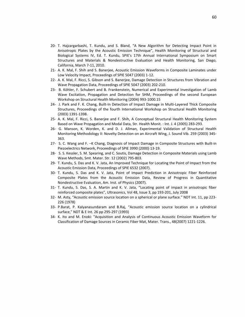
60

20- T. Hajzargarbashi, T. Kundu, and S. Bland, “A New Algorithm for Detecting Impact Point in Anisotropic Plates by the Acoustic Emission Technique”, Health Monitoring of Structural and Biological Systems IV, Ed. T. Kundu, SPIE's 17th Annual International Symposium on Smart Structures and Materials & Nondestructive Evaluation and Health Monitoring, San Diego, California, March 7-11, 2010.

21- A. K. Mal, F. Shih and S. Banerjee, Acoustic Emission Waveforms in Composite Laminates under Low Velocity Impact, Proceedings of SPIE 5047 (2003) 1-12.

22- A. K. Mal, F. Ricci, S. Gibson and S. Banerjee, Damage Detection in Structures from Vibration and Wave Propagation Data, Proceedings of SPIE 5047 (2003) 202-210.

23- B. Köhler, F. Schubert and B. Frankenstein, Numerical and Experimental Investigation of Lamb Wave Excitation, Propagation and Detection for SHM, Proceedings of the second European Workshop on Structural Health Monitoring (2004) 993-1000.15

24- J. Park and F. K. Chang, Built-In Detection of Impact Damage in Multi-Layered Thick Composite Structures, Proceedings of the fourth International Workshop on Structural Health Monitoring (2003) 1391-1398.

25- A. K. Mal, F. Ricci, S. Banerjee and F. Shih, A Conceptual Structural Health Monitoring System Based on Wave Propagation and Modal Data, Str. Health Monit. : Int. J. 4 (2005) 283-293.

26- G. Manson, K. Worden, K. and D. J. Allman, Experimental Validation of Structural Health Monitoring Methodology II: Novelty Detection on an Aircraft Wing, J. Sound Vib. 259 (2003) 345-363.

27- S. C. Wang and F. –K Chang, Diagnosis of Impact Damage in Composite Structures with Built-in Piezoelectrics Network, Proceedings of SPIE 3990 (2000) 13-19.

28- S. S. Kessler, S. M. Spearing, and C. Soutis, Damage Detection in Composite Materials using Lamb Wave Methods, Smt. Mater. Str. 12 (2002) 795-803.

29- T. Kundu, S. Das and K. V. Jata, An Improved Technique for Locating the Point of Impact from the Acoustic Emission Data, Proceedings of SPIE 6532 (2007).

30- T. Kundu, S. Das and K. V. Jata, Point of Impact Prediction in Anisotropic Fiber Reinforced Composite Plates from the Acoustic Emission Data, Review of Progress in Quantitative Nondestructive Evaluation, Am. Inst. of Physics (2007).

31- T. Kundu, S. Das, S. A. Martin and K. V. Jata, “Locating point of impact in anisotropic fiber reinforced composite plates”, Ultrasonics, Vol 48, Issue 3, pp 193-201, July 2008

32- M. Asty, “Acoustic emission source location on a spherical or plane surface.” NDT Int. 11, pp 223-226 (1978)

33- P.Barat, P. Kalyanasundaram and B.Raj, “Acoustic emission source location on a cylindrical surface,” NDT & E Int. 26 pp 295-297 (1993)

34- K. Ito and M. Enoki: "Acquisition and Analysis of Continuous Acoustic Emission Waveform for Classification of Damage Sources in Ceramic Fiber Mat, Mater. Trans., 48(2007) 1221-1226.

61

APPENDIX C

DETECTING THE POINT OF IMPACT ON AN ANISOTROPIC

CYLINDRICAL SURFACE USING ONLY FOUR ACOUSTIC

SENSORS

This work has been published in IWSHM Conference proceedings:

T. Hajzargarbashi, H. Nakatani, T. Kundu and N. Takeda,” Detecting the

Point of Impact on an Anisotropic Cylindrical Surface using only Four

Acoustic Sensors”, The 8th International Workshop on Structural Health

Monitoring, Sep 13-15, 2011, Stanford University, Vol. 1, pp. 562-569,

2011.

62

Abstract:

An optimization based technique for detecting the point of impact on isotropic and

anisotropic plates was developed by Kundu and his associates. Acoustic sensors attached to

the plate record the arrival times of Lamb waves generated at the impact point. An objective

function is then minimized to obtain the impact location[1-3]. Recently this technique has

been extended to the cylindrical geometry. This optimization based technique has been

tested on both flat plates and cylindrical shells made of aluminum[4]. In this paper the

impact point on an anisotropic cylindrical shell geometry made of carbon fiber reinforced

composite is investigated. One shortcoming of the previous method of requiring a large

number of acoustic sensors to obtain the direction dependent velocity profile is also

overcome here. In the new method the velocity profile in the anisotropic shell is obtained

using only four sensors. Predicted points of impact on the anisotropic cylindrical shell are

compared with the actual impact points. Good agreement between the two sets is observed.

Key Words: Lamb Wave, Impact, Acoustic Emission, Passive Monitoring, Cylindrical

Surface, Optimization.

6. Introduction

Localizing the point of impact on an anisotropic plate is necessary for detecting and

repairing the delamination or any other type of defect arising from an impact. A popular

method for detecting the point of impact is the acoustic emission technique. This technique

has been mostly used on isotropic plates. Using passive sensors attached to the isotropic

plate the point of impact can be localized by the acoustic emission method following the

triangulation technique [5,6]. For efficiently monitoring the plate the sensors need to be

placed near the critical locations of the plate [7-12]. In anisotropic plates the wave speed is

not the same in all directions and therefore the triangulation technique does not work [1, 13,

14], Kundu et al. [1] proposed an alternative method which is based on minimizing a

nonlinear error function to find the point of impact. The original objective function proposed

in that reference was modified by Kundu et al. [15] to overcome the singularity problem

associated with that function. It was then improved further [2, 3] to make the objective

function more efficient and less sensitive to errors in the time of flight measurement. The

number of sensors was increased to get more accurate results [2, 3, 14]. All these

investigations were carried out on a flat plate. This investigation is extended to cylindrical

structures in this paper. Cylindrical structures have many applications in industry. Most fuel

cylinders have cylindrical geometry. Main bodies of space shuttles and air plane fuselages

also have cylindrical shapes.

63

In 1978 Asty [16] used the triangulation technique to detect the point of impact on a

spherical surface, then in 1993 Barat et al. [17] detected the point of impact on a cylindrical

surface using the triangulation technique; none of these techniques have been

experimentally verified. As it has been mentioned before the triangulation technique does

not work for an anisotropic cylinder for which the wave speed is a function of the wave

propagation direction. Kundu et al. detected the point of impact on an aluminum cylindrical

shell by the acoustic emission technique [4]. In this paper a similar technique is applied to an

anisotropic cylindrical geometry made of fiber reinforced composite. The cylindrical

coordinates of the attached sensors and the times of flight of the arriving waves at the sensor

locations are used to detect the point of impact. The direction dependent velocity profile in

the cylinder wall is experimentally obtained from the sensors attached to the cylinder. In the

previous technique one shortcoming of obtaining the direction dependent velocity profile in

an anisotropic plate was the need to have a large number of sensors attached to the plate.

This shortcoming is avoided here by introducing a new method for obtaining the velocity

profile.

7. Formulation 7.1. Introducing the optimization equation

Let the time of detection of the acoustic signal at the i-th receiving station be . If the

time of impact be then the travel time for the signal from the impact point to the station

location is (1)

Note that in (1) both and are defined in the same time of reference. Cylindrical

coordinates of the receiving sensors S1, S2, S3 and S4 are (r, θ1, z1), (r, θ2, z2), (r, θ3, z3) and

(r, θ4, z4), respectively and the impact point coordinate is (r, θ0, z0) in which r is the radius of

the cylinder. The sensors can be attached on the outer or inner surface of the cylinder. The

impact point can be also on the outer or inner surface. For the cylindrical arc θ is the angle

measured from a reference axis, and z is the vertical coordinate of the sensors, as shown in

Figure 1(a). In order to be able to find the distance between the sensor and the point of

impact the cylindrical surface is unwrapped to form a flat surface; it makes the calculation

easier. In this manner the cylindrical surface becomes a rectangular plate with two side

lengths equal to rxθtotal and the length of the cylinder. In which θtotal is the angle formed by

the cylindrical arc at its center. As it has been shown in Figure 1(b), when the cylindrical

surface is unwrapped to form a flat surface the coordinates of the sensors and the impact

point are mapped into the transformed coordinate system in which the coordinates of the

attached sensors and the impact point can be expressed as (rxθi, zi). In this manner after

converting cylindrical coordinates to Cartesian coordinates the distance between the point of

impact and the i-th sensor can be found easily,

√( ) ( )

i=1,2,3,4 (2)

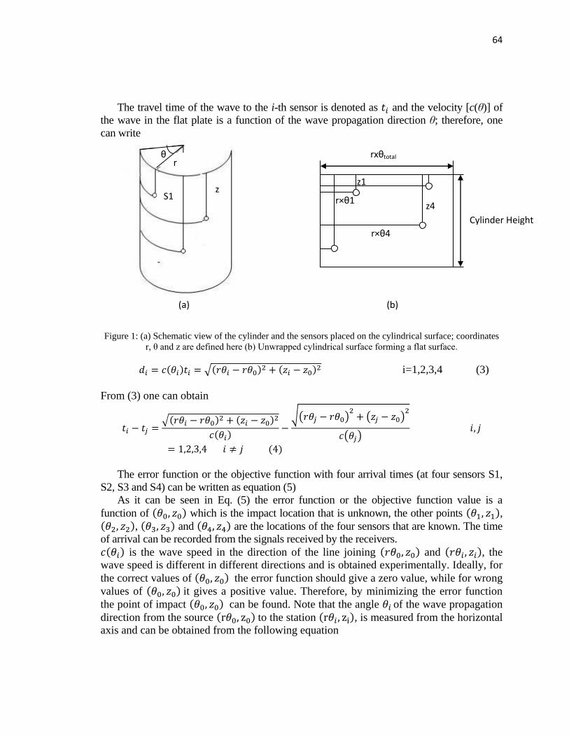
64

The travel time of the wave to the i-th sensor is denoted as and the velocity [c(θ)] of

the wave in the flat plate is a function of the wave propagation direction θ; therefore, one

can write

Figure 1: (a) Schematic view of the cylinder and the sensors placed on the cylindrical surface; coordinates

r, θ and z are defined here (b) Unwrapped cylindrical surface forming a flat surface.

( ) √( ) ( )

i=1,2,3,4 (3)

From (3) one can obtain

√( )

( )

( ) √( )

( )

( )

( )

The error function or the objective function with four arrival times (at four sensors S1,

S2, S3 and S4) can be written as equation (5)

As it can be seen in Eq. (5) the error function or the objective function value is a

function of ( ) which is the impact location that is unknown, the other points ( ), ( ), ( ) and ( ) are the locations of the four sensors that are known. The time

of arrival can be recorded from the signals received by the receivers.

( ) is the wave speed in the direction of the line joining ( ) and ( ), the

wave speed is different in different directions and is obtained experimentally. Ideally, for

the correct values of ( ) the error function should give a zero value, while for wrong

values of ( ) it gives a positive value. Therefore, by minimizing the error function

the point of impact ( ) can be found. Note that the angle of the wave propagation

direction from the source ( ) to the station ( ), is measured from the horizontal

axis and can be obtained from the following equation

r

z

θ

S1

(a) (b) (a) (b)

r×θ1

z1

rxθtotal

Cylinder Height

r×θ4

z4

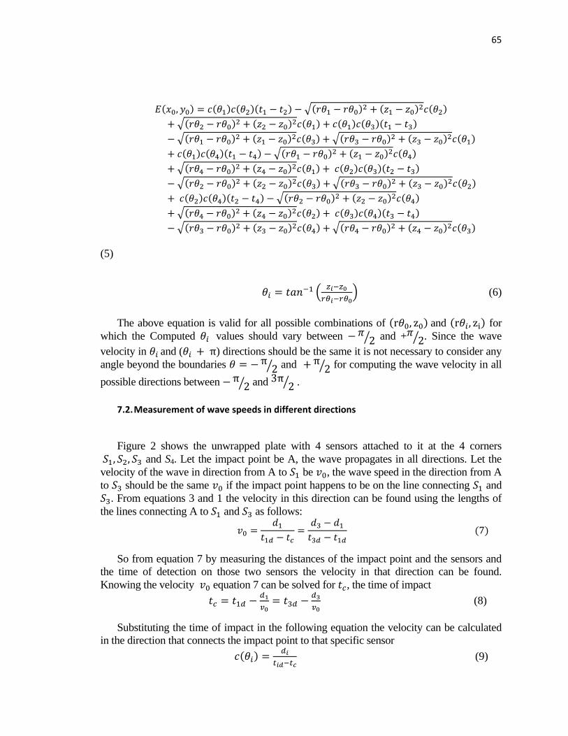
65

( ) ( ) ( )( ) √( ) ( )

( )

√( ) ( )

( ) ( ) ( )( )

√( ) ( )

( ) √( ) ( )

( )

( ) ( )( ) √( ) ( )

( )

√( ) ( )

( ) ( ) ( )( )

√( ) ( )

( ) √( ) ( )

( )

( ) ( )( ) √( ) ( )

( )

√( ) ( )

( ) ( ) ( )( )

√( ) ( )

( ) √( ) ( )

( )

(5)

(

) (6)

The above equation is valid for all possible combinations of ( ) and ( ) for

which the Computed values should vary between ⁄ and + ⁄ . Since the wave

velocity in and ( ) directions should be the same it is not necessary to consider any

angle beyond the boundaries ⁄ and ⁄ for computing the wave velocity in all

possible directions between ⁄ and ⁄ .

7.2. Measurement of wave speeds in different directions

Figure 2 shows the unwrapped plate with 4 sensors attached to it at the 4 corners

and S4. Let the impact point be A, the wave propagates in all directions. Let the

velocity of the wave in direction from A to be , the wave speed in the direction from A

to should be the same if the impact point happens to be on the line connecting and

. From equations 3 and 1 the velocity in this direction can be found using the lengths of

the lines connecting A to and as follows:

( )

So from equation 7 by measuring the distances of the impact point and the sensors and

the time of detection on those two sensors the velocity in that direction can be found.

Knowing the velocity equation 7 can be solved for , the time of impact

(8)

Substituting the time of impact in the following equation the velocity can be calculated

in the direction that connects the impact point to that specific sensor

( )

(9)

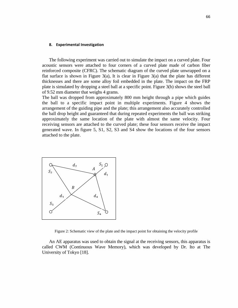
66

8. Experimental Investigation

The following experiment was carried out to simulate the impact on a curved plate. Four

acoustic sensors were attached to four corners of a curved plate made of carbon fiber

reinforced composite (CFRC). The schematic diagram of the curved plate unwrapped on a

flat surface is shown in Figure 3(a), It is clear in Figure 3(a) that the plate has different

thicknesses and there are some alloy foil embedded in the plate. The impact on the FRP

plate is simulated by dropping a steel ball at a specific point. Figure 3(b) shows the steel ball

of 9.52 mm diameter that weighs 4 grams.

The ball was dropped from approximately 800 mm height through a pipe which guides

the ball to a specific impact point in multiple experiments. Figure 4 shows the

arrangement of the guiding pipe and the plate; this arrangement also accurately controlled

the ball drop height and guaranteed that during repeated experiments the ball was striking

approximately the same location of the plate with almost the same velocity. Four

receiving sensors are attached to the curved plate; these four sensors receive the impact

generated wave. In figure 5, S1, S2, S3 and S4 show the locations of the four sensors

attached to the plate.

Figure 2: Schematic view of the plate and the impact point for obtaining the velocity profile

An AE apparatus was used to obtain the signal at the receiving sensors, this apparatus is

called CWM (Continuous Wave Memory), which was developed by Dr. Ito at The

University of Tokyo [18].

𝑆

𝑑

𝑆

𝑑

𝐴

𝑑

𝑑

𝑆

𝑆

𝐵

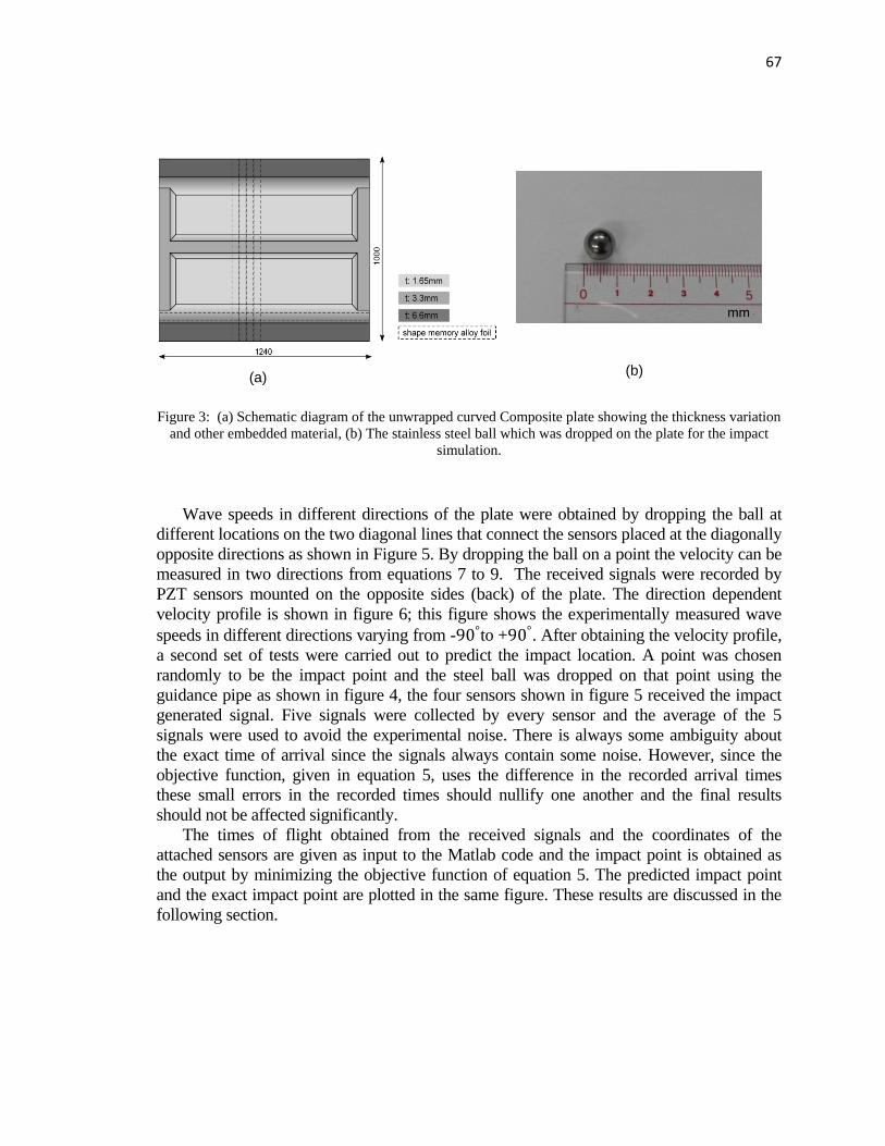
67

Figure 3: (a) Schematic diagram of the unwrapped curved Composite plate showing the thickness variation

and other embedded material, (b) The stainless steel ball which was dropped on the plate for the impact

simulation.

Wave speeds in different directions of the plate were obtained by dropping the ball at

different locations on the two diagonal lines that connect the sensors placed at the diagonally

opposite directions as shown in Figure 5. By dropping the ball on a point the velocity can be

measured in two directions from equations 7 to 9. The received signals were recorded by

PZT sensors mounted on the opposite sides (back) of the plate. The direction dependent

velocity profile is shown in figure 6; this figure shows the experimentally measured wave

speeds in different directions varying from - to + . After obtaining the velocity profile,

a second set of tests were carried out to predict the impact location. A point was chosen

randomly to be the impact point and the steel ball was dropped on that point using the

guidance pipe as shown in figure 4, the four sensors shown in figure 5 received the impact

generated signal. Five signals were collected by every sensor and the average of the 5

signals were used to avoid the experimental noise. There is always some ambiguity about

the exact time of arrival since the signals always contain some noise. However, since the

objective function, given in equation 5, uses the difference in the recorded arrival times

these small errors in the recorded times should nullify one another and the final results

should not be affected significantly.

The times of flight obtained from the received signals and the coordinates of the

attached sensors are given as input to the Matlab code and the impact point is obtained as

the output by minimizing the objective function of equation 5. The predicted impact point

and the exact impact point are plotted in the same figure. These results are discussed in the

following section.

(a) (b)

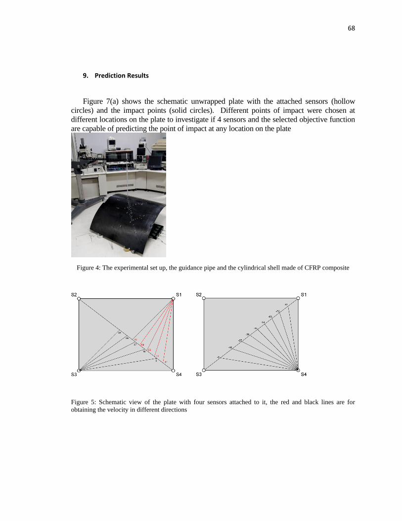
68

9. Prediction Results

Figure 7(a) shows the schematic unwrapped plate with the attached sensors (hollow

circles) and the impact points (solid circles). Different points of impact were chosen at

different locations on the plate to investigate if 4 sensors and the selected objective function

are capable of predicting the point of impact at any location on the plate

Figure 4: The experimental set up, the guidance pipe and the cylindrical shell made of CFRP composite

Figure 5: Schematic view of the plate with four sensors attached to it, the red and black lines are for

obtaining the velocity in different directions

69

Figure 6: Experimentally obtained wave velocity in the curved composite plate as a function of the

propagation direction

4000

4500

5000

5500

6000

6500

-90 -80 -70 -60 -50 -40 -30 -20 -10 0 10 20 30 40 50 60 70 80 90 100

Angle (Degree)

Vel

oci

ty

(m/s

)

y

x

S4(1.08,0.15

)

S3(0.16,0.15

)

A(0.76,0.3

5)

C(0.52,0.69

)

S1(1.08,0.85

)

S2(0.16,0.85

)

B(0.71,0.75

)

(a) (b)

(c) (d)

70

Figure 7: (a) Schematic view of the unwrapped Composite plate with the sensors (S1, S2, S3 and S4)

attached to it. Random impact points are marked by A, B and C, Predicted results (dots) and exact impact

points (stars) for tests A, B and C are shown in figures (b), (c) and (d), respectively.

Predicted impact points are shown in figures 7 (b), (c) and (d) for the impact at locations

A, B and C (shown in figure 7(a)), respectively. The dots in these figures show the

predictions and the stars show the exact impact locations. It can be seen that the predicted

points are very close to the exact impact points in all 3 tests.

10. Conclusions

The optimization based method for detecting the impact point on isotropic and

anisotropic plates developed by Kundu and his associates [1, 2] is extended to the

cylindrical geometry. An objective function is defined that uses the cylindrical coordinates

of the attached sensors and the arrival times at the sensors to locate the point of impact by

minimizing an objective function. A new method that uses only four sensors for obtaining

the wave speeds in different directions is introduced. The technique is experimentally

verified by carrying out impact localization tests on cylindrical plates. The results show that

by minimizing the objective function introduced in this paper the impact point can be

correctly predicted.

REFERENCES

1. T. Kundu, S. Das and K. V. Jata, “Point of Impact Prediction in Isotropic and Anisotropic Plates from the

Acoustic Emission Data”, Journal of the Acoustical Society of America, Vol. 122 (4), pp. 2057-2066, 2007

2. T. Hajzargarbashi, T. Kundu, and S. Bland, “An improved algorithm for detecting point of impact in

anisotropic inhomogeneous plates” Ultrasonics, Vol 51,pp. 317-324, 2011

3. T. Hajzargarbashi, T. Kundu, and S. Bland, “A New Algorithm for Detecting Impact Point in Anisotropic

Plates by the Acoustic Emission Technique”, Proceeding of SPIE 7650, 7650C (2010)

4. T. Hajzargarbashi, H. Nakatani, T. Kundu and N. Takeda, “Detecting the Point of Impact on a Cylindrical

Plate by the Acoustic Emission Technique”,Proceeding of SPIE 7981, 79810U, (2011).

5. A. K. Mal, F. Shih and S. Banerjee, Acoustic Emission Waveforms in Composite Laminates under Low

Velocity Impact, Proceedings of SPIE 5047 (2003) 1-12.

6. A. K. Mal, F. Ricci, S. Gibson and S. Banerjee, Damage Detection in Structures from Vibration and Wave

Propagation Data, Proceedings of SPIE 5047 (2003) 202-210.

7. B. Köhler, F. Schubert and B. Frankenstein, Numerical and Experimental Investigation of Lamb Wave

Excitation, Propagation and Detection for SHM, Proceedings of the second European Workshop on

Structural Health Monitoring (2004) 993-1000.15

8. J. Park and F. K. Chang, Built-In Detection of Impact Damage in Multi-Layered Thick Composite

Structures, Proceedings of the fourth International Workshop on Structural Health Monitoring (2003)

1391-1398.

9. A. K. Mal, F. Ricci, S. Banerjee and F. Shih, A Conceptual Structural Health Monitoring System Based on

Wave Propagation and Modal Data, Str. Health Monit. : Int. J. 4 (2005) 283-293.

10. G. Manson, K. Worden, K. and D. J. Allman, Experimental Validation of Structural Health Monitoring

Methodology II: Novelty Detection on an Aircraft Wing, J. Sound Vib. 259 (2003) 345-363.

71

11. S. C. Wang and F. –K Chang, Diagnosis of Impact Damage in Composite Structures with Built-in

Piezoelectrics Network, Proceedings of SPIE 3990 (2000) 13-19.

12. S. S. Kessler, S. M. Spearing, and C. Soutis, Damage Detection in Composite Materials using Lamb Wave

Methods, Smt. Mater. Str. 12 (2002) 795-803.

13. T. Kundu, S. Das and K. V. Jata, An Improved Technique for Locating the Point of Impact from the

Acoustic Emission Data, Proceedings of SPIE 6532 (2007).

14. T. Kundu, S. Das and K. V. Jata, Point of Impact Prediction in Anisotropic Fiber Reinforced Composite

Plates from the Acoustic Emission Data, Review of Progress in Quantitative Nondestructive Evaluation,

Am. Inst. of Physics (2007).

15. T. Kundu, S. Das, S. A. Martin and K. V. Jata, “Locating point of impact in anisotropic fiber reinforced

composite plates”, Ultrasonics, Vol 48, Issue 3, pp 193-201, July 2008

16. M. Asty, “Acoustic emission source location on a spherical or plane surface.” NDT Int. 11, pp 223-226

(1978)

17. P.Barat, P. Kalyanasundaram and B.Raj, “Acoustic emission source location on a cylindrical surface,” NDT

& E Int. 26 pp 295-297 (1993)

18. K. Ito and M. Enoki: "Acquisition and Analysis of Continuous Acoustic Emission Waveform for

Classification of Damage Sources in Ceramic Fiber Mat, Mater. Trans., 48(2007) 1221-1226.

72

APPENDIX D

IMPACT LOCALIZATION ON A CYLINDRICAL PLATE

BY A NEAR-FIELD BEAMFORMING ANALYSIS

H. Nakatani, T. Hajzargarbashi T. Kundu and N. Takeda, “Impact

Localization on a Cylindrical Plate by a Near-Field Beamforming Analysis”,

Accepted to be published in SPIE Proceeding (2012).

73

Abstract:

Detecting the point of impact is of great importance in health monitoring of structural

systems especially those used in aviation fields. One candidate for the impact localization

method is the beamforming analysis proposed by McLaskey et al. [1], it requires only a

small array of 4 to 8 sensors. This technique is considered to be more suitable than

conventional time difference of arrival (TDOA) method because it is not influenced by

noise and dispersion of waves generated by the impact event. This beamforming method

with 4 sensors is extended here to thin cylindrical structures using guided Lamb waves. A

difficulty involved is that this technique which assumes constant wave speed in all

propagation directions does not work for anisotropic plates and cylinders. In order to

overcome this problem, the beamforming analysis in conjunction with an optimization

technique that introduces an objective function or error function is developed in this

study. The proposed technique is experimentally verified by comparing the predicted

values with the exact points of impact on a cylindrical FRP plate.

1. Introduction:

Source localization by the acoustic emission technique is necessary to identify the hot

spots of the structure. The localization of impact on a structure can direct further, more

detailed nondestructive analysis of the specified region. The popular and conventional

acoustic emission technique uses the time difference of arrival in the triangulation

technique. This method has been widely used on isotropic homogenous structures [2, 3]

and also has been extended to anisotropic plates [4]. The time difference of arrival has

been validated and used extensively for detecting the point of impact or crack growth

dislocation movement, fiber breakage and fiber matrix debonding. The time difference of

arrival scheme utilizes the difference in the times of arrival of various wave modes in

order to determine the source coordinates via triangulation. In acoustic emission work,

the arrivals of different wave modes are not easily identifiable so in order to get the time

74

difference of arrival usually the fastest propagating wave is determined for use in

acoustic emission source location methods. The source location method is typically

formulated as an inverse problem which relies on the very accurate determination of the

arrival time. In principle, it is also possible to solve the inverse problem such a way that

small errors in the arrival time do not produce large errors in the prediction [4].

One shortcoming of the conventional time difference method is that as the distance

between the source and the sensor increases the signal becomes more spread out and the

first arrival time of the weak signal becomes increasingly difficult to measure accurately.

For overcoming this problem usually the number of sensors on the surface is increased to

get a stronger signal at the sensor position.

Another difficulty of using the conventional method is encountered for anisotropic

structures for which the wave velocities in different directions are different. This

shortcoming is overcome here.

In the method described here a small array of sensors spaced closely together are used

instead of a distributed array of sensors on the surface. In the frequency range of interest,

all closely located sensors detect waves that propagate along similar paths and have been

affected by similar attenuation and scattering. This beamforming method was proposed

by McLaskey et al. [1] who used it for detecting the impact location in large concrete

structures. He et al. [5] then extended this method to the near-field beamforming in thin

isotropic plates[5]. They validated the effectiveness of the method by series of rotor-

stator rubbing experiments [5].

This paper attempts to explore the possibility of using the near-field beamforming

acoustic emission technique to locate the point of impact on a FRP cylindrical shell

which is an anisotropic structure. The theoretical fundamental is explained briefly and

then the method is validated by dropping a ball to simulate the impact on different

locations of a FRP cylinder. The results show that the beamforming acoustic emission

technique is an alternative method to the conventional acoustic emission technique.

75

2. Theoretical fundamentals:

Time delay beamforming is a method of filtering in both time and space, and the analysis

techniques are relevant to the study of signals generated by propagating waves. In

beamforming technique the assumption is that the characteristics of waves incident on the

array are relatively constant normal to their direction of propagation [6]. Under this

fundamental assumption, a signal recorded by one sensor in an array is expected to be a

time-delayed replica of a signal recorded by a neighboring sensor in that array. Acoustic

emission sources are usually considered point sources, so the delayed replica assumption

is only valid if the distance between the source and sensors is large compared to the

distance between the neighboring sensors.

Many different formulations for array signal processing have been tried out. Delay- and

sum is a simple and effective array signal processing algorithm utilized in beamfroming

technique [7]. This method is a generalized cross-correclation of the signal received in

array of sensors.

Comparing the distance between acoustic emission source and array of sensors, the

analysis schemes based on beamforming techniques can be classified as near-field and

far-field methods. The wave front form of the signal is assumed spherical due to the

transmission characteristic of waves. A common rule of thumb is that the near field

sources are located at a distance of

(1)

Where r is the distance from an arbitrary origin of the array, L is the largest dimension of

the array and λ is the wavelength [5,8].

Here the study is on the near-field source location in which the wave front is assumed to

be spherical. Figure 1 illustrates the incident spherical wave when the array of sensors

are attached to the plate.

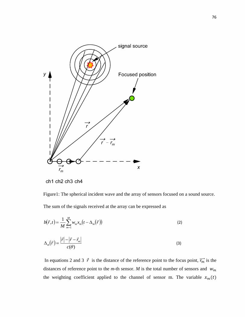
76

Figure1: The spherical incident wave and the array of sensors focused on a sound source.

The sum of the signals received at the array can be expressed as

M

m

mmm rtxwM

trb1

1,

(2)

)(c

rrrr

m

m

(3)

In equations 2 and 3 ⃗ is the distance of the reference point to the focus point, ⃗⃗⃗⃗⃗ is the

distances of reference point to the m-th sensor. M is the total number of sensors and

the weighting coefficient applied to the channel of sensor m. The variable ( )

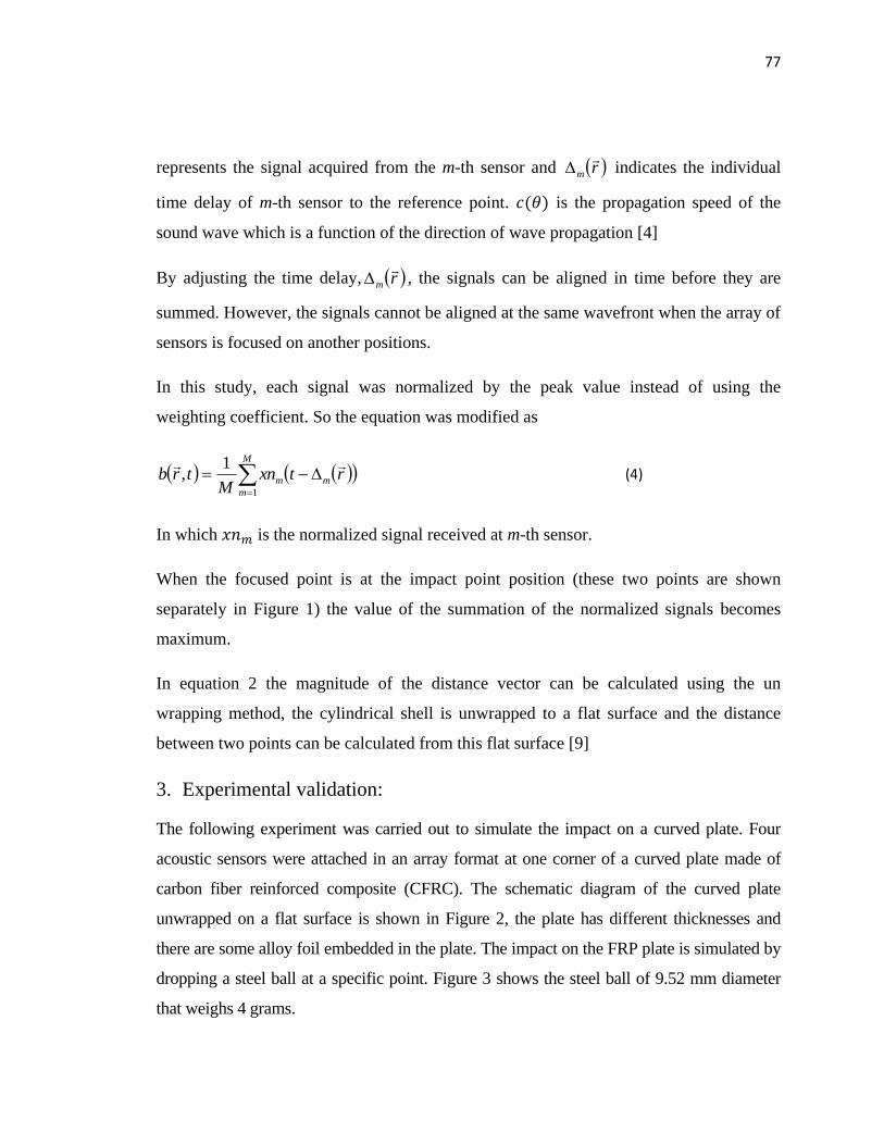
77

represents the signal acquired from the m-th sensor and rm

indicates the individual

time delay of m-th sensor to the reference point. ( ) is the propagation speed of the

sound wave which is a function of the direction of wave propagation [4]

By adjusting the time delay, rm

, the signals can be aligned in time before they are

summed. However, the signals cannot be aligned at the same wavefront when the array of

sensors is focused on another positions.

In this study, each signal was normalized by the peak value instead of using the

weighting coefficient. So the equation was modified as

M

m

mm rtxnM

trb1

1,

(4)

In which is the normalized signal received at m-th sensor.

When the focused point is at the impact point position (these two points are shown

separately in Figure 1) the value of the summation of the normalized signals becomes

maximum.

In equation 2 the magnitude of the distance vector can be calculated using the un

wrapping method, the cylindrical shell is unwrapped to a flat surface and the distance

between two points can be calculated from this flat surface [9]

3. Experimental validation:

The following experiment was carried out to simulate the impact on a curved plate. Four

acoustic sensors were attached in an array format at one corner of a curved plate made of

carbon fiber reinforced composite (CFRC). The schematic diagram of the curved plate

unwrapped on a flat surface is shown in Figure 2, the plate has different thicknesses and

there are some alloy foil embedded in the plate. The impact on the FRP plate is simulated by

dropping a steel ball at a specific point. Figure 3 shows the steel ball of 9.52 mm diameter

that weighs 4 grams.

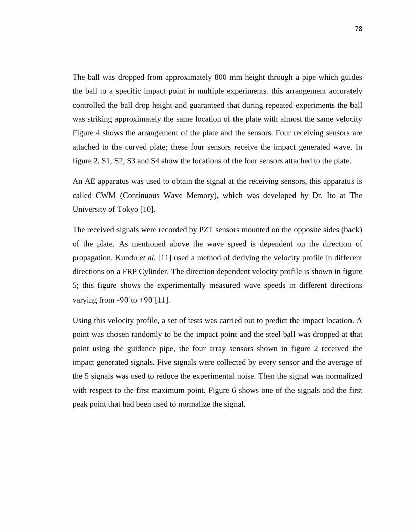
78

The ball was dropped from approximately 800 mm height through a pipe which guides

the ball to a specific impact point in multiple experiments. this arrangement accurately

controlled the ball drop height and guaranteed that during repeated experiments the ball

was striking approximately the same location of the plate with almost the same velocity

Figure 4 shows the arrangement of the plate and the sensors. Four receiving sensors are

attached to the curved plate; these four sensors receive the impact generated wave. In

figure 2, S1, S2, S3 and S4 show the locations of the four sensors attached to the plate.

An AE apparatus was used to obtain the signal at the receiving sensors, this apparatus is

called CWM (Continuous Wave Memory), which was developed by Dr. Ito at The

University of Tokyo [10].

The received signals were recorded by PZT sensors mounted on the opposite sides (back)

of the plate. As mentioned above the wave speed is dependent on the direction of

propagation. Kundu et al. [11] used a method of deriving the velocity profile in different

directions on a FRP Cylinder. The direction dependent velocity profile is shown in figure

5; this figure shows the experimentally measured wave speeds in different directions

varying from - to + [11].

Using this velocity profile, a set of tests was carried out to predict the impact location. A

point was chosen randomly to be the impact point and the steel ball was dropped at that

point using the guidance pipe, the four array sensors shown in figure 2 received the

impact generated signals. Five signals were collected by every sensor and the average of

the 5 signals was used to reduce the experimental noise. Then the signal was normalized

with respect to the first maximum point. Figure 6 shows one of the signals and the first

peak point that had been used to normalize the signal.

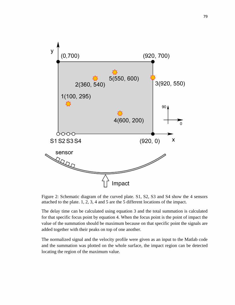
79

Figure 2: Schematic diagram of the curved plate. S1, S2, S3 and S4 show the 4 sensors

attached to the plate. 1, 2, 3, 4 and 5 are the 5 different locations of the impact.

The delay time can be calculated using equation 3 and the total summation is calculated

for that specific focus point by equation 4. When the focus point is the point of impact the

value of the summation should be maximum because on that specific point the signals are

added together with their peaks on top of one another.

The normalized signal and the velocity profile were given as an input to the Matlab code

and the summation was plotted on the whole surface, the impact region can be detected

locating the region of the maximum value.

80

Figure 3: The stainless steel ball which has been used to simulate the drop.

Figure 4: The FRP cylindrical plate with sensors attached to it

Stainless steel ball 9.52mm dia. 4gr

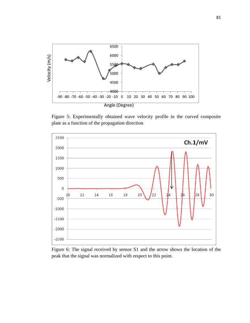
81

Figure 5: Experimentally obtained wave velocity profile in the curved composite

plate as a function of the propagation direction

Figure 6: The signal received by sensor S1 and the arrow shows the location of the

peak that the signal was normalized with respect to this point.

4000

4500

5000

5500

6000

6500

-90 -80 -70 -60 -50 -40 -30 -20 -10 0 10 20 30 40 50 60 70 80 90 100

Angle (Degree)

Vel

oci

ty (

m/s

)

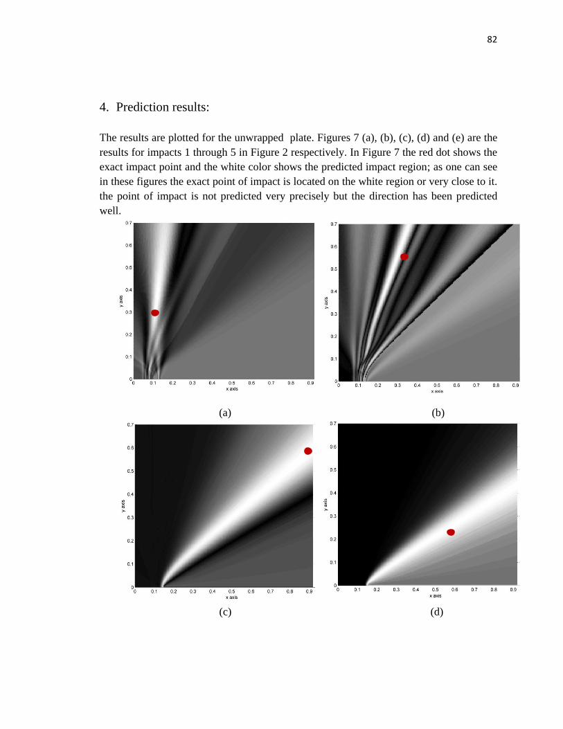
82

4. Prediction results:

The results are plotted for the unwrapped plate. Figures 7 (a), (b), (c), (d) and (e) are the

results for impacts 1 through 5 in Figure 2 respectively. In Figure 7 the red dot shows the

exact impact point and the white color shows the predicted impact region; as one can see

in these figures the exact point of impact is located on the white region or very close to it.

the point of impact is not predicted very precisely but the direction has been predicted

well.

\

(a) (b)

(c) (d)

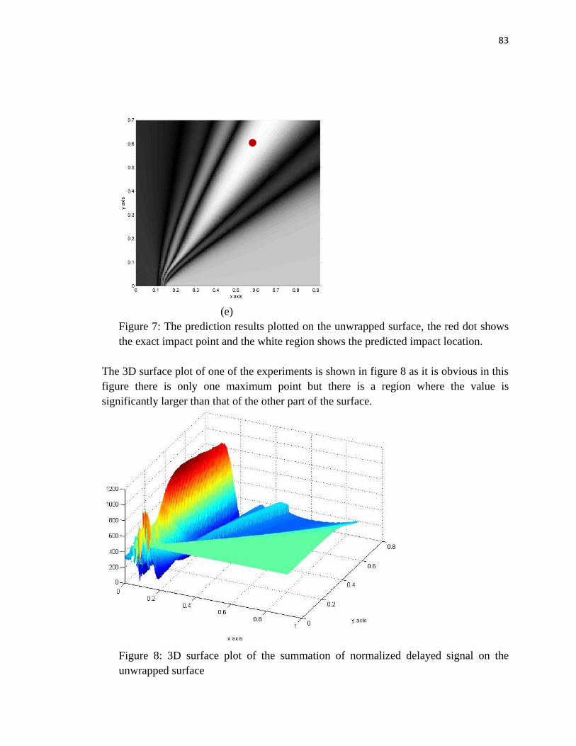
83

(e)

Figure 7: The prediction results plotted on the unwrapped surface, the red dot shows

the exact impact point and the white region shows the predicted impact location.

The 3D surface plot of one of the experiments is shown in figure 8 as it is obvious in this

figure there is only one maximum point but there is a region where the value is

significantly larger than that of the other part of the surface.

Figure 8: 3D surface plot of the summation of normalized delayed signal on the

unwrapped surface

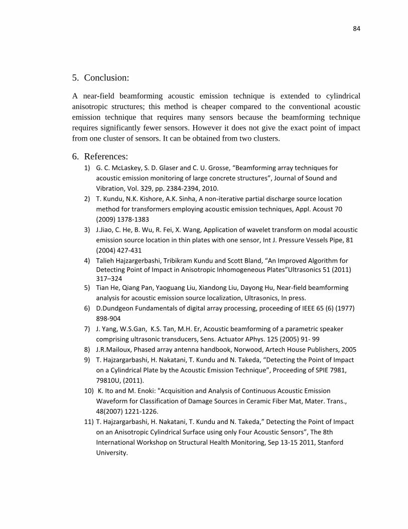
84

5. Conclusion:

A near-field beamforming acoustic emission technique is extended to cylindrical

anisotropic structures; this method is cheaper compared to the conventional acoustic

emission technique that requires many sensors because the beamforming technique

requires significantly fewer sensors. However it does not give the exact point of impact

from one cluster of sensors. It can be obtained from two clusters.

6. References:

1) G. C. McLaskey, S. D. Glaser and C. U. Grosse, “Beamforming array techniques for

acoustic emission monitoring of large concrete structures”, Journal of Sound and

Vibration, Vol. 329, pp. 2384-2394, 2010.

2) T. Kundu, N.K. Kishore, A.K. Sinha, A non-iterative partial discharge source location

method for transformers employing acoustic emission techniques, Appl. Acoust 70

(2009) 1378-1383

3) J.Jiao, C. He, B. Wu, R. Fei, X. Wang, Application of wavelet transform on modal acoustic

emission source location in thin plates with one sensor, Int J. Pressure Vessels Pipe, 81

(2004) 427-431

4) Talieh Hajzargerbashi, Tribikram Kundu and Scott Bland, “An Improved Algorithm for Detecting Point of Impact in Anisotropic Inhomogeneous Plates”Ultrasonics 51 (2011) 317–324

5) Tian He, Qiang Pan, Yaoguang Liu, Xiandong Liu, Dayong Hu, Near-field beamforming

analysis for acoustic emission source localization, Ultrasonics, In press.

6) D.Dundgeon Fundamentals of digital array processing, proceeding of IEEE 65 (6) (1977)

898-904

7) J. Yang, W.S.Gan, K.S. Tan, M.H. Er, Acoustic beamforming of a parametric speaker

comprising ultrasonic transducers, Sens. Actuator APhys. 125 (2005) 91- 99

8) J.R.Mailoux, Phased array antenna handbook, Norwood, Artech House Publishers, 2005

9) T. Hajzargarbashi, H. Nakatani, T. Kundu and N. Takeda, “Detecting the Point of Impact

on a Cylindrical Plate by the Acoustic Emission Technique”, Proceeding of SPIE 7981,

79810U, (2011).

10) K. Ito and M. Enoki: "Acquisition and Analysis of Continuous Acoustic Emission

Waveform for Classification of Damage Sources in Ceramic Fiber Mat, Mater. Trans.,

48(2007) 1221-1226.

11) T. Hajzargarbashi, H. Nakatani, T. Kundu and N. Takeda,” Detecting the Point of Impact

on an Anisotropic Cylindrical Surface using only Four Acoustic Sensors”, The 8th

International Workshop on Structural Health Monitoring, Sep 13-15 2011, Stanford

University.

85

APPENDIX E

SCATTERING OF FOCUSED ULTRASONIC BEAMS BY

TWO SPHERICAL CAVITIES IN CLOSE PROXIMITY

This work has been published in IEEE Transaction on Ultrasonics,

Ferroelectrics and Frequency control:

Talieh Hajzargerbashi, Ehsan Kabiri Rahani and Tribikram

Kundu,“Scattering of focused ultrasonic beams by multiple cavities” IEEE

Transaction on Ultrasonics, Ferroelectrics and Frequency control, Vol 58,No

8, pp-1619-1628, 2011

86

Abstract:

Ultrasonic fields generated by one and two spherical cavities placed in front of a point

focused acoustic lens are modeled by the semi-analytical distributed point source method

(DPSM). Results are generated by properly considering the interaction effect between

two cavities placed in the focused ultrasonic field. The interaction effect between the two

cavities prohibits the linear superposition of single cavity solutions to obtain the solution

for the two cavities placed in close proximity. Therefore, although some analytical and

semi-analytical solutions are available for the single cavity in a focused ultrasonic field,

those solutions cannot be simply superimposed for solving the two-cavity problem even

for a linear elastic material. Solution of this problem is necessary to get an idea about

when two cavities placed in close proximity can be distinguished by an acoustic lens and

when it is not possible. How the reflected ultrasonic energy from two small cavities and

one big cavity compares is also investigated.

I. INTRODUCTION:

The propagation of waves through a medium containing strong scatterers is ubiquitous in

nature [1]. This is because generally inhomogeneities are always found in materials.

These inhomogeneities locally change the acoustic properties of the material. Air cavities

and solid inclusions in molten and solid metals are some examples of these

inhomogeneities. A large number of papers have been published on elastic wave

propagation through materials containing inclusions. In particular, scattering of elastic

waves by spherical inhomogeneities_(e.g. voids, inclusions and other types of defect) has

87

been investigated because of its importance in nondestructive testing and exploratory

geophysics [2]. Detection and characterization of floating cavities in a liquid medium is

important for both materials science and medical applications, such as for characterizing

air bubbles in molten metal and blood.

In physics and optics the multiple scattering theory has been studied extensively

(electron propagation in a random potential or propagation of light in turbid media) [3-7].

A good review of the acoustic wave scattering by multiple scatterers can be also found in

Tourin et al. [8] However, interaction between multiple cavities in a focused field has not

been investigated extensively either in acoustic or in electromagnetic literature.

In 80s and 90s investigators tried to use ultrasonic pulse-echo techniques with

buffer rod to detect bubbles [9, 10] but because of the lack of resolution and SNR (signal

to noise ratio) it was not very successful. In order to increase the quality of detection in

late 90s spherical focused lenses were used by Ihara et al. [11-13]. They used 10 MHz

focused ultrasound to detect 20 to 80 m diameter particles in molten zinc at 650oC.

Another common method for detecting and sizing gas bubbles is pulsed Doppler

ultrasound for moving bubbles [14].

Acoustic microscopes use focused ultrasonic beams at high frequencies to image

small inclusions, cavities and cracks. The interaction between a spherical cavity in a

solid or a fluid medium and a focused ultrasonic beam has been investigated analytically

earlier by Lobkis et al.[15, 16] and Zinin et al.[17, 18]. These analytical investigations

have several restrictions that make the analytical method applicable only to high

frequency focused signal interacting with a small spherical cavity having a small

88

eccentricity or offset from the focal point; when it comes to solid the solution is even

more restrictive such as signal duration should be sufficiently short such that the

longitudinal and transverse waves scattered by the cavity are separated in time and thus

can be analyzed separately [15-18]. Without these assumptions there is no analytical

solution for this problem. The single cavity problem has been solved semi-analytically

with fewer restrictions by Placko et al. [19]. They used a newly developed mesh-free

technique called Distributed Point Source Method or DPSM to model acoustic

microscope lenses at high frequencies. The DPSM technique for solving ultrasonic,

electrostatic and electromagnetic problems was developed by Placko and Kundu [20, 21].

Using DPSM, the ultrasonic field has been computed in fluid media [22-24] and solid

structures [25-27]. Kundu et al. [28] successfully modeled the ultrasonic field generated

in front of an acoustic lens in a perfect fluid medium in absence of any inhomogeneity or

anomaly. Placko et al. [19] solved the problem of interaction between a focused

ultrasonic beam and a cavity using DPSM. In this research the scattering of the ultrasonic

field is investigated when two cavities are present in the medium including the interaction

effect between the two. Some simplifying assumptions that can be used for solving

scattering by a single cavity are not applicable to two-cavity case. The field computed by

a single cavity and two cavities placed in close proximity are compared to study the

resolution of the lens; or in other words, what minimum distance is necessary for the lens

to clearly distinguish the two cavities. Effect of the cavity size and the ultrasonic wave

length on the resolution limit is also investigated.

II. THEORETICAL FORMULATION

89

To obtain accurate information about the size and location of cavities using an acoustic

microscope, it is necessary to correctly model the interaction between the ultrasonic beam

generated by the acoustic microscope lens and multiple cavities. Even for the single

cavity case there is no analytical solution available for high eccentricity (distance

between the lens focal point and the cavity center), non-spherical shape of the cavity, or

when the cavity radius is not significantly smaller than the focal distance, so this problem

must be solved using numerical or semi-analytical techniques.

Finite element method is probably the most popular method for modeling the

engineering problems [29-35]. However, the finite dlement method requires a fine

meshing at high frequencies. As a result, 3D problems at high frequencies are

computationally very time consuming and sometimes impossible to solve [36]. The

alternative semi analytical approach that has been used by Plako et al. [19] is the mesh-

free technique called DPSM. In DPSM a number of point sources are distributed behind

the transducer face to model the transducer. The pressure field at position y in the fluid,

due to the point sources at position x distributed over surface S, can be expressed as [20]

S

fxdS

r

rikByp )(

4

)exp()(

(1)

In which B is proportional to the source velocity amplitude.

When the transducer surface is divided into small areas associated with the

source points then the above integral can be written in terms of the summation as follows:

90

N

m m

mf

m

N

m m

mf

mr

rikA

r

rikS

Byp

11

)exp()exp(

4)(

(2)

In which is the source strength of the m-th point source. Source strengths can be

assumed uniform over a transducer face for uniform vibration of the transducer. N is the

total number of point sources, is the distance between the m-th point source and the

target point or the observation point, kf is the wave number which has a real value for

materials without any attenuation or a complex value for materials with attenuation. In

this analysis kf is considered real. Superimposing the contributions of these source points

the pressure field for spherical and cylindrical focused lenses have been computed when

there is no inhomogeneity in front of the transducer [28]. DPSM has been used for

computing the scattered field generated by single spherical cavity [19] considering two

groups of point sources, one group on the boundary of the cavity and the second group on

the boundary of the lens. Final results are obtained by superimposing the contributions of

these two groups of point sources.

A major simplifying assumption for computing the scattered field by a small

cavity placed at a relatively large distance from the lens is to separately analyze the

incident field and the scattered field [19]. From the incident field analysis the pressure at

the cavity surface position is obtained in absence of the cavity then the negative of that

pressure field is applied on the cavity surface to get the scattered field. Although this

approach works well for the single cavity analysis it is not acceptable when two cavities

are present in close proximity. For the two-cavity case in addition to the lens generated

incident field the scattered field produced by one cavity affects the other cavity as well.

91

To model the ultrasonic field in presence of two cavities, the acoustic lens and the

two cavities must be analyzed simultaneously, not one cavity at a time. The point sources

need to be distributed on the two cavities as well as along the surface of the lens as shown

in Figure 1. The ultrasonic field at point P is obtained by superimposing the contributions

of all point sources.

Pressure and displacement fields at point P due to a single point source at a distance r

from point P is given by Banerjee and Kundu [25],

rik

f

jj

j

rik

f

f

er

ikr

xyu

r

ep

1

4

4

22

(3)

Where p is the pressure and ju is the displacement vector; the point source is located at

coordinate xj and the coordinate of point P is yj.

Several points like point P in Figure 1 are placed on the lens-fluid interface and

the cavity surfaces. The pressure and displacement fields at these points can be obtained

from Equation (3) for point sources of unit strength. For point sources with unknown

source strengths AS, AB1 and AB2 the pressure and displacement expressions at point P

contain these unknown source strengths. A matrix equation in the following form is

obtained by simultaneously satisfying the specified velocity (or displacement) boundary

conditions on the lens surface and the stress-free boundary conditions on the cavity

surfaces [21].

92

[

] {

} {

} (4)

If m, n1 and n2 point sources are used to model the lens surface and the cavity surfaces

then AS, AB1 and AB2 in Eq. (4) should have m, n1 and n2 elements, respectively. Vectors

VS, PB1 and PB2 on the right hand side are obtained from the prescribed boundary

conditions. For example, we can assume that the pressures PB1 and PB2 on the surface of

the two cavities are zero and the transducer surface velocity VS is uniform. VS vector

contains the prescribed velocity values on the lens surface at m points where small

spheres representing the point sources touch the lens surface. Similarly vectors PB1 and

PB2 contain the pressure values at n1 and n2 points on the cavity surfaces where the point

source spheres touch the cavity surfaces. Matrices M and Q relate the source strengths to

the particle velocity and pressure values, respectively. Note that MSS, MSB1, QB1S, MSB2,

QB2S, QB1B1, QB2B2 and QB1B2 matrices have dimensions m by m, m by n1, n1 by m, m by

n2, n2 by m, n1 by n1, n2 by n2 and n1 by n2, respectively. To obtain the source

strengths the system of equations given in Eq. (4) are to be solved.

If the resultant velocity on the transducer surface is specified as {VS} and the

pressure on the cavity surfaces are zero then the source strengths are obtained from the

following system of equations

[

] {

} { } (5)

93

However, if the pressure {PS} on the transducer surface instead of the velocity is

specified then the source strengths are obtained from the following equations

[

] {

} { } (6)

Both equations (5) and (6) require solution of a system of linear equations. This solution

is valid for any size of two cavities placed at any location. Interested readers are referred

to [20, 36] for the detailed forms of M and Q matrices used in Eqs. (5) and (6). After

obtaining the frequency domain solution as described above the time domain solution can

be obtained by applying Fast Fourier Transform (FFT) to the frequency domain solution

[37].

III. NUMERICAL RESULTS

Following the above formulation, the ultrasonic field in front of an acoustic lens (or

transducer) in presence of two (or more) cavities can be computed by solving a matrix

equation. The computed field for the two-cavity prolem is compared with the field

generated in absence of the cavity and in presence of only one cavity to see the effect of

the second cavity in close proximity.

The opening angle of the point focused lens (also known as the lens angle) and

the lens radius are 100o and 20 mm, respectively. The lens (or the transducer) is excited

at 1 MHz frequency. Note that modeling this large lens at 1 MHz frequency is equivalent

to modeling a much smaller lens, say 50 m radius with 100o lens opening angle,

94

operating at 400 MHz frequency because in these two cases the lens radius/wavelength

ratio is the same.

The lens surface is modeled by 4003 point sources, distributed slightly behind the

lens face as shown in Figure 1. The number of point sources is selected based on the

convergence criterion that the spacing between two neighboring point sources is less than

one-third wavelength [20]. Two cavities are placed with a horizontal spacing d between

the two cavity centers. These two cavities are denoted as the right and left cavities based

on their relative orientations. When the cavities are moved relative to the acoustic lens

whose position remains unchanged then the locations of the two cavities are denoted by

the coordinates of the center of the right cavity and the horizontal spacing between the

two cavity centers. If the distance between these two centers in Figure 1 is d then the

cavity locations for this figure are denoted as (0, y1) with a spacing d, implying the center

of the right cavity is located at coordinate point (0, y1) and the coordinate of the left

cavity center is (-d, y1). Origin of the coordinate system coincides with the focal point of

the lens. When only one cavity is analyzed then the left cavity is dropped.

The pressure fields computed in the fluid in presence of one cavity and two

cavities are shown in Figures 2a and 2b, respectively. For the case of one cavity the

cavity is placed at the focal point of the lens (0, 0) and the pressure field is plotted. For

the two-cavity modeling the left cavity is placed at (-0.4, 0) mm while the right cavity is

placed at the focal point (0, 0), as shown in Figure 1; corresponding pressure field is

95

shown in Figure 2b. One can see that the pressure field has changed relatively more on

the left side of the focal point, due to the presence of the second cavity, as expected.

It is then investigated if two small cavities close to each other have the same

effect as a bigger cavity at the same location. The pressure field is plotted in Figure 2c for

the case of one bigger cavity (of double diameter). The center of the bigger cavity is not

at the central axis of the lens but at (-0.2, 0) mm, which is the midpoint of two smaller

cavities of Figure 2b. One can see in this figure that the pressure fields look similar but

there are some differences between these two fields near the cavity location. However,

the two fields shown in Figures 2b and 2c are not distinguishable when moving away

from the cavities.

Two cavities of Figure 2b are then moved further away from each other and the

computed pressure fields are shown in Figure 3. It is evident in this figure that as the

distance between the cavity centers increases from 0.8 mm (Fig. 3a) to 2 mm (Fig. 3d)

the pressure field close to the cavities changes significantly. It should be noted in Figures

3a through 3d that the interference fringes just below the cavities diminishes as the

distance between the two cavities increases.

It should also be pointed out that the visible changes in the pressure field very

close to the cavities, as seen in Figures 2 and 3, do not help us much in detecting the

cavity, distinguishing the two cavities, or estimating the distance between the two cavities

because the sensing element is generally not placed so close to the cavity locations. For

cavity detection by the reflection mode acoustic microscope the acoustic lens is used for

96

transmitting the ultrasonic beam as well as receiving the reflected signal from the cavity.

The pressure field generated by the reflected ultrasonic energy from the cavity is

integrated over the lens surface to compute the acoustic force sensed by the lens due to

the reflected signal and is compared with the transmitted force, as was done by Placko et

al.[19] for the single cavity detection. It is shown there that the acoustic force (or the

integration of the pressure on the lens surface) varies noticeably as the cavity is moved

horizontally (right and left) or vertically (up and down) from the focal point. The same

method is used here to show the difference between the acoustic force when only one or

two cavities are present in front of the lens.

Figure 4 shows the normalized force sensed by the acoustic lens that is generated

by the ultrasonic beam reflected from the cavities. It is plotted as a function of the

vertical distance of the cavities from the horizontal plane going through the focal point.

The upward movement of the cavities is considered positive while the negative sign is

assigned to the downward movement. This sign convention is followed since in Figure 1

the y-coordinate is shown positive upward. In Figure 4 the solid line shows the reflected

force sensed by the acoustic lens from a cavity of radius 0.1 mm. The distance is denoted

as zero when the cavity center coincides with the focal point and it is positive when it

moves away from the acoustic lens. Note that the maximum value of the force is

obtained when the cavity is moved 0.2 mm towards the lens from the focal plane and it

decreases as the cavity moves up or down from that position; the dashed line shows the

reflected force from the two cavities with their centers 0.4 mm apart. As mentioned

before for the two-cavity case a distance equal to zero implies the center of the right

97

cavity coinciding with the focal point while the left cavity’s center is 0.4 mm left of the

focal point at coordinate (-0.4, 0) mm. The positive value of the distance indicates that

the two cavities moving away from the lens keeping the horizontal spacing between the

cavities unchanged. For this case also the maximum value is obtained when the cavities

are about 0.2 mm closer to the lens from the focal plane and it decays as the cavities

move away from this position. Note that the reflected force is stronger for the case of

two cavities in comparison to the single cavity case. The third curve – the dashed-dotted

line with markers – shows the reflected force from a single bigger cavity of radius 0.2

mm. In this case the maximum value of the reflected force is located at about the same

distance as the other two curves and its peak value is close to that of the two-cavity case.

The main difference between the force variations from the single big cavity and two

smaller cavities is that a slightly sharper dip is noticed for the two-cavity case.

In figures 5, 6 and 7 reflected forces are plotted when the cavities are placed on

the horizontal focal plane and moved in this plane to the right and left of the focal point.

In these figures three curves are plotted – one corresponding to a single small cavity

(continuous line), the second curve (dashed line) is for two small cavities separated by

some distance and the third curve (dashed-dotted line with markers) is for the single

bigger cavity. The x axis shows the horizontal distance of the right cavity from the focal

point. When there is only one cavity then there is no left cavity and the distance is

measured from the center of the cavity to the focal point. As indicated before the

distance from the focal point is positive when the cavity moves to the right and it is

negative when the movement is to the left. The y axis shows the reflected force which

98

has been normalized with respect to the maximum value. In all three figures (5, 6 and 7)

the maximum force is obtained from the single big cavity of radius 0.2 mm. The solid and

dashed-dotted curves corresponding to smaller and bigger single cavities, respectively

show perfect symmetry about the focal position as expected. The force value diminishes

as the cavity moves to the right or left by more than 1 mm.

The dashed curves that correspond to the two-cavity cases show some interesting

features. When the cavities are 0.4 mm apart the dashed curve is almost identical to the

dashed-dotted curve (see Figure 5). The only difference is that the peaks of the two

curves are off by 0.2 mm. This is because the midpoint of the two cavities is 0.2 mm off

from the center of the right cavity. If the distance of this midpoint (instead of the

distance of the center of the right cavity) from the focal point were plotted along the

horizontal axis then these two curves would have almost coincided. Clearly in this case

the acoustic lens cannot distinguish between one big cavity and two small cavities placed

close to each other.

In figures 6 and 7 the distance between the two cavities is increased to 0.8 mm

and 1.2 mm, respectively. In Figure 6 the maximum force from the two cavities is found

to be smaller than that from one big cavity but greater than that from one cavity of same

size. Note that as expected the symmetry line of the dashed curve in figure 6 is moved by

a distance of 0.4 mm to the right. 0.8 mm separation between the two cavities also

increases the width of the dashed curve by about 0.8 mm compared to the other two

curves. In figure 7 we see that as the distance between the centers of the two cavities is

99

increased to 1.2 mm clearly two peaks appear and the cavities become distinguishable.

Peak values for a single cavity and two cavities matched in this case because the cavities

are 1.2 mm apart while the influence of a single cavity beyond a distance of 1 mm from

its center is negligible. As expected in Figure 7 the line of symmetry for the dashed

curve moves 0.6 mm to the right. Theoretical curves for the single cavity problem

geometries are also plotted in Figure 7. Note that the theoretical curves match well with

the DPSM solutions.

Next it is investigated how the resolution power of the focused transducer

depends on the cavity size and the signal frequency. With this goal in mind figures 6 and

7 are regenerated after changing the cavity size and signal frequency. In Figure 8 the

spacing between the two cavity centers is kept constant at 0.8 mm as in Figure 6 but the

cavity diameters are reduced by a factor of 2 (Figure 8a), and increased by a factor of 2

(Figure 8b), then signal frequency is reduced by a factor of 2 (Figure 8c) and increased

by a factor of 2 (Figure 8d) in comparison to those values of Figure 6. Figure 9 is similar

to Figure 8 but the difference is that in Figure 9 the spacing between the two cavity

centers is 1.2 mm as in Figure 7 instead of 0.8 mm.

Figures 6, 8a and 8b show that when the cavity centers are 0.8 mm apart then they

cannot be distinguished even when the cavity diameters are reduced by 75% while

keeping the signal frequency unchanged. However, from Figures 6, 8c and 8d one can

see that for 0.5 MHz signal frequency (Figure 8c) one cavity of 0.2 mm diameter and two

cavities of 0.1 mm diameter each gives almost identical curves. When the signal

100

frequency is increased to 1 MHz (Figure 6) then these two curves show some difference

but still two peaks cannot be observed for the two-cavity case. Finally, when the

frequency is increased to 2 MHz (Figure 8d) then the lens can distinguish between the

two cavities – the curve shows two distinct peaks for the two-cavity geometry.

Next figures 7, 9a and 9b are compared. In all three cases two distinct peaks can

be seen for the two-cavity case indicating that even when the cavity diameter is increased

by 300% keeping the spacing between the cavity centers and the signal frequency

unchanged the resolution power of the lens is not compromised. However, when the

signal frequency is reduced to 0.5 MHz (Figure 9c) two distinct peaks disappear even for

1.2 mm spacing. As the frequency is increased to 1 MHz (Figure 7) two peaks can be

observed although they partly overlap and when the frequency is increased further to 2

MHz (Figure 9d) then two well separated peaks corresponding to two cavities can be

clearly seen.

Therefore, from figures 6, 7, 8 and 9 one can conclude that the capability of a

focused acoustic lens to distinguish between two cavities in close proximity does not

depend on the cavity size but it is strongly influenced by the signal frequency. From the

single cavity results presented in figures 6 to 9 it can be seen that for 0.5 MHz, 1 MHz

and 2 MHz signal frequency the effect of the cavity (influence zone) is extended to 2

mm, 1 mm and 0.5 mm, respectively from the center of the cavity. Therefore, if the

spacing between two cavity centers exceeds this influence zone then the two cavities can

be distinctly identified. Note that the wavelengths corresponding to these three

101

frequencies are 3 mm, 1.5 mm and 0.75 mm respectively. Therefore, the resolution

power of the point focused acoustic lens is approximately two-third of the wavelength.

As a result, cavities at a spacing of 0.4 mm could not be distinguished by any of these

three frequencies, while at 0.8 mm spacing only 2 MHz signal could distinguish the two

cavities and at 1.2 mm spacing both 2 MHz and 1 MHz signals could distinguish the

cavities but 0.5 MHz signal could not.

IV. CONCLUSIONS

Ultrasonic fields in front of a point focused lens in presence of single and two spherical

cavities are computed by semi-analytical DPSM formulation. The results are obtained

without ignoring any interaction effect between the two cavities or the cavities and the

lens. The main difference between the single cavity analyses available in the literature

and the two-cavity analysis presented here is that in the two-cavity case the presence of

the second cavity in close proximity affects the solution due to the first cavity. Because

of this interaction effect between the two cavities the total solution is not simply the

linear superposition of the two single cavity solutions. To correctly take into account this

interaction effect the two cavities should be considered concurrently in the model and all

boundary conditions on the lens and cavity surfaces must be satisfied simultaneously, as

done here. As mentioned earlier many simplifying assumptions for the single cavity

analysis cannot be used for solving the multiple-cavity problem.

102

The computed results show that when the distance between the two cavities

exceeds the radius of the influence zone (it is a function of the signal frequency) the

acoustic lens can distinguish the two cavities; otherwise the responses from two small

cavities and one big cavity show no difference. Therefore, for two cavities in close

proximity (within the influence zone or resolution limit of the acoustic lens) one cannot

conclude if the response is generated by single or multiple cavities. The resolution limit

does not depend on the cavity size but it is strongly influenced by the signal frequency. It

is approximately two-third of the wavelength.

Even when the spacing between two neighboring cavities is less than the

resolution limit of the lens, if the approximate size of the cavities is known then it is

possible to identify the presence of more than one cavity within the resolution limit since

the strength of the reflected signal depends on the cavity size. If the detected signal

strength exceeds the expected value for the known size of the cavity then one can

conclude that more than one cavity must be present with an inter-cavity spacing less than

the resolution limit of the lens.

Acknowledgement This research was financially supported by a research grant from the Air Force Office of

Scientific Research, contract number: FA9550-08-1-0318, Program Managers Dr. Victor

Giurgiutiu and Dr. David Stargel.

References:

103

[1] Sheng, P., "Introduction to Wave Scattering, Localization, and Mesoscopic

Phenomena ", Academic Press, Boston, 1995.

[2] Seyyed M. Hasheminejad1 and Seyyed A. Badsar, " Elastic Wave Scattering by Two

Spherical Inclusions in a Poroelastic Medium ", J. Engrg. Mech. Volume 131, Issue 9, pp.

953-965, Sep. 2005.

[3]Y. Kuga and A. Ishimaru, "Retroreflectance from a dense distribution of spherical

particles," J. Opt. Soc. Am. A 1, 831–835, 1984.

[4] Leung Tsang and Akira Ishimaru, "Backscattering enhancement of random discrete

scatterers," J. Opt. Soc. Am. A 1, 836-839, 1984.

[5] Van Albada M P and Lagendijk Ad, “Observation of Weak Localization of Light in a

Random Medium”, Phys. Rev. Lett. 55, 2692–2695, 1985.

[6]Wolf P.E and Maret G, “Weak Localization and Coherent Backscattering of Photons

in Disordered Media”, Phys. Rev. Lett. 55, 2696–2699, 1985.

[7]E. Akkermans, P.E. Wolf, R. Maynard and G. Maret, “Theoretical study of the

coherent backscattering of light by disordered media, “ J. de Physique (France), 49, 77-

98, 1988.

[8]Tourin, A., Fink, M., and Derode, A. “Multiple scattering of sound.” Waves Random

Media, vol.10, pp 31–60, Oct 2000.

[9]N. D. G. Mountford , P. Hahlin, S. Lee and I. D. Sommerville, “Progress in the

Development of an Ultrasonic Sensor for the Measurement of Liquid Metal Cleanliness”

Proceedings of the 74th Steel making Conference, Warrendale, PA, 1991, pp. 773.

104

[10]T. L. Mansfield, “Ultrasonic Technology for. Measuring Molten Aluminum Quality”

Materials Evaluation, 41, pp. 743-747, 1983.

[11] I. Ihara, C. –K. Jen and D. R. Franca,”Materials Evaluation Using Long Clad Buffer

Rods”, IEEE International Ultrasonic Symposium Proceedings, Sendai, 1998, pp. 803-

809.

[12] I. Ihara, C. –K. Jen and D. R. Franca, “Detection of Inclusion in Molten Metal by

Focused Ultrasonic Wave”, Japan Journal of Applied Physics, 39(5B), pp. 3152-3153,

2000.

[13] I. Ihara, C. –K. Jen and D. R. Franca,” C-scan imaging in molten zinc by focused

ultrasonic waves”, Journal of the Acoustical Society of America, 107(2), pp. 1042-1044,

2000.

[14] K. Hatteland and B. K. H. Semb, “Gas Bubble Detection in Fluid Lines by means of

Pulsed Doppler Ultrasound”, Scandinavian Journal of Thoracic Cardiovascular Surgery,

19(2), pp. 119-123, 1985.

[15] O. I. Lobkis, T. Kundu and P.V. Zinin, "A Theoretical Analysis of Acoustic

Microscopy of Spherical Cavities", Wave Motion, Vol.21 (2), pp.183-201, 1995.

[16] O. I. Lobkis and P.V. Zinin, “Acoustic Microscopy of Spherical Objects Theoretical

Approach”, Acoustic Letters, 14, pp.168-172, 1990.

[17] P. V. Zinin and W. Weise, “Chapter 11: Theory and applications of acoustic

microscopy”, Ultrasonic Nondestructive Evaluation: Engineering and Biological Material

Characterization. Ed. T. Kundu, Pub. CRC Press, Boca Raton, Fl, pp. 654-724, 2004.

105

[18] P. V. Zinin, W. Weise, O. Lobkis, O. Kolosov and S. Boseck, “Fourier optics

analysis of spherical particles image formation in reflection acoustic microscopy”, Optik,

98(2), pp.45-60, 1994.

[19] D. Placko, T. Yangagita, E. Kabiri Rahani and T. Kundu, “Mesh-free modeling of

the interaction between a point-focused acoustic lens and a cavity”, IEEE Transactions on

Ultrasonics, Ferroelectrics, and Frequency Control, Vol.57(6), pp. 1396-1404, 2010

[20] D. Placko and T. Kundu, “Chapter 2: Modeling of ultrasonic field by distributed

point source method”, [Ultrasonic Nondestructive Evaluation: Engineering and

Biological Material Characterization], Ed. T. Kundu, Pub. CRC Press, pp.143-202, 2004.

[21] D. Placko and T. Kundu, Eds. [DPSM for Modeling Engineering Problems], John

Wiley & Sons, Hoboken, New Jersey, USA, ISBN: 978 0 471 73314 0, 1-832, 2007.

[22] D. Placko and T. Kundu, "A theoretical study of magnetic and ultrasonic sensors:

dependence of magnetic potential and acoustic pressure on the sensor geometry",

Advanced NDE for Structural and Biological Health Monitoring, Proceedings of SPIE,

Ed. T. Kundu, SPIE's 6th Annual International Symposium on NDE for Health

Monitoring and Diagnostics, March 4-8, 2001, Newport Beach, California, 4335, pp. 52-

62.

[23] R. Ahmad, T. Kundu and D. Placko, "Modeling of phased array transducers",

Journal of the Acoustical Society of America, 117(4 Pt 1), 1762-1776, 2005.

[24] S. Banerjee, T. Kundu and D. Placko, “Ultrasonic field modelling in multilayered

fluid structures using DPSM technique”, ASME Journal of Applied Mechanics, 73 (4),

598-609, 2006

106

[25] S. Banerjee and T. Kundu, “Chapter 4: Advanced Applications of Distributed Point

Source Method - Ultrasonic Field Modeling in Solid media”, [DPSM for Modeling

Engineering Problems], Eds. D. Placko and T. Kundu, John Wiley & Sons, 143-229,

2007.

[26] S. Banerjee and T. Kundu, “Semi-analytical modeling of ultrasonic fields in solids

with internal anomalies immersed in a fluid”, Wave Motion, 45 (5), pp.581-595, 2008.

[27] S. Das, C. M. Dao, S. Banerjee and T. Kundu, “DPSM modeling for studying

interaction between bounded ultrasonic beams and corrugated plates”, IEEE Transactions

on Ultrasonics, Ferroelectrics and Frequency Control, 54(9), pp. 1860-1872, 2007.

[28] . Kundu, D. Placko, T. Yanagita and S. Sathish, “Micro Interferometric Acoustic

Lens: Mesh-Free Modeling with Experimental Verification”, Health Monitoring of

Structural and Biological Systems III, Ed. T. Kundu, SPIE's 16th Annual International

Symposium on Smart Structures and Materials & Nondestructive Evaluation and Health

Monitoring, San Diego, California, March 9-12, 2009, Vol. 7295(2), pp. 72951E-1 to

72950M-11.

[29] W. Lord, R. Ludwig and Z. You, “Developments in ultrasonic modeling with finite

element analysis”, Journal of Nondestructive Evaluation, 9(2-3), pp. 129-143, 1990.

[30] R. Ludwig, D. Moore and W. Lord, “A comparative study of analytical and

numerical transient force excitations on an elastic half-space”, IEEE Transactions on

Ultrasonics Ferroelectrics and Frequency Control, 36(3), pp. 342-350, 1989.

107

[31] Z. You, M. Lusk, W. Lord and R. Ludwig, “Numerical simulation of ultrasonic

wave propagation in anisotropic and attenuative solid materials”, IEEE Transactions on

Ultrasonics Ferroelectrics and Frequency Control, 38(5), pp. 436-445, 1991

[32] J. Zhu and A. H. Shah, “A hybrid method for transient wave scattering by flaws in

composite plates”, International Journal of Solids and Structures, 34(14), pp. 1719-1734,

1997

[33] P. Kudela, M. Krawczuk and W. Ostachowicz, “Wave propagation modelling in 1D

structures using spectral finite elements”, Journal of Sound and Vibration, 300(1-2), pp.

88-100, 2007.

[34] M. Mitra and S. Gopalakrishnan, “Wavelet based spectral finite element modelling

and detection of de-lamination in composite beams”, Proc R Soc London - Ser A,

462(2070), pp. 1721-1740, 2006

[35] M. Mitra and S. Gopalakrishnan, “Wavelet Based 2-D spectral finite element

formulation for wave propagation analysis in isotropic plates”, CMES: Computer Model

Eng Science, 15(1), pp. 49-68, 2006.

[36] T. Kundu, D. Placko, E. Kabiri Rahani, T. Yanagita and C. M. Dao, “Ultrasonic

Field Modeling: A Comparison between Analytical, Semi-Analytical and Numerical

Techniques” IEEE Transactions on Ultrasonics, Ferroelectric and Frequency Control,

Vol. 57(12), pp. 2795-2807, 2010.

[37] S. Das, S. Banerjee and T. Kundu, “Modeling of Transient Ultrasonic Wave

Propagation in an Elastic Half-Space using Distributed Point Source Method”, Health

Monitoring of Structural and Biological Systems, Ed. T. Kundu, SPIE's 17th

Annual

108

International Symposium on Smart Structures and Materials & Nondestructive

Evaluation and Health Monitoring, San Diego, California, March 7-11,2010, Vol. 7650,

pp.76501G-1 to 76501G-12.

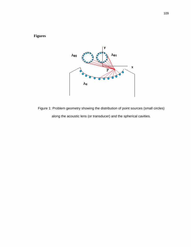
109

Figures

Figure 1: Problem geometry showing the distribution of point sources (small circles)

along the acoustic lens (or transducer) and the spherical cavities.

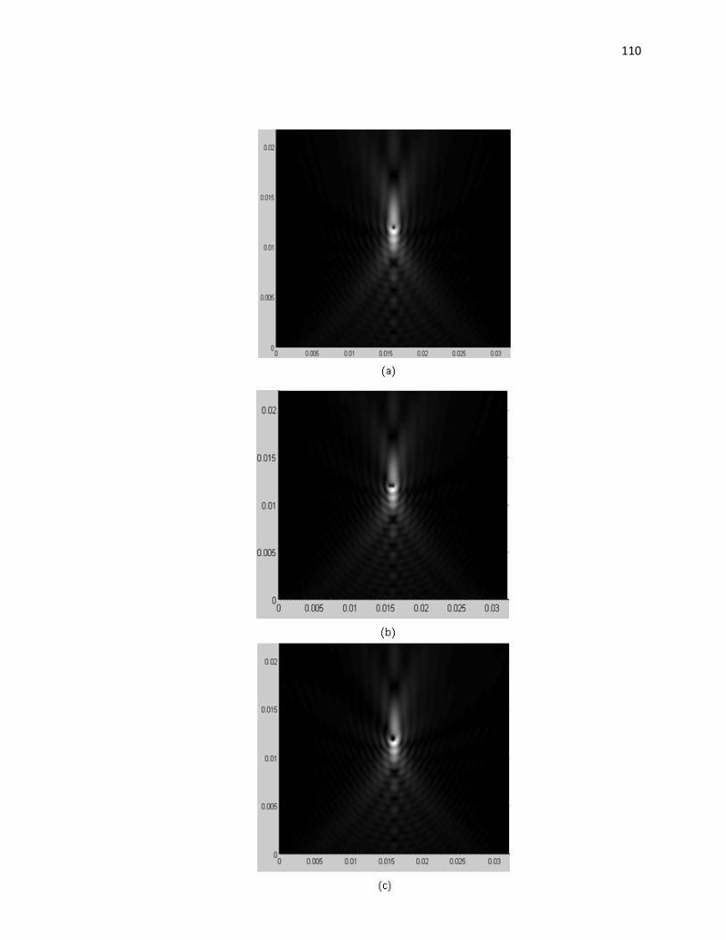
110

111

Figure 2: Computed pressure fields in front of the acoustic lens – (a) in presence of one

small spherical cavity (radius = 0.1 mm) located at the focal point, (b) in presence of two

small cavities (radius = 0.1 mm) one located at the focal point and the other one 0.4 mm

left of the focal point;, (c) in presence of one bigger cavity (radius = 0.2 mm) located at

0.2 mm left of the focal point. Numbers along the horizontal and vertical axes are given

in meters and denote positions of the field points in a Cartesian coordinate system

whose origin coincides with the bottom left corner of the figure. Scales are slightly

different in x and y directions. Note the changes in the pressure field slightly left of the

focal point

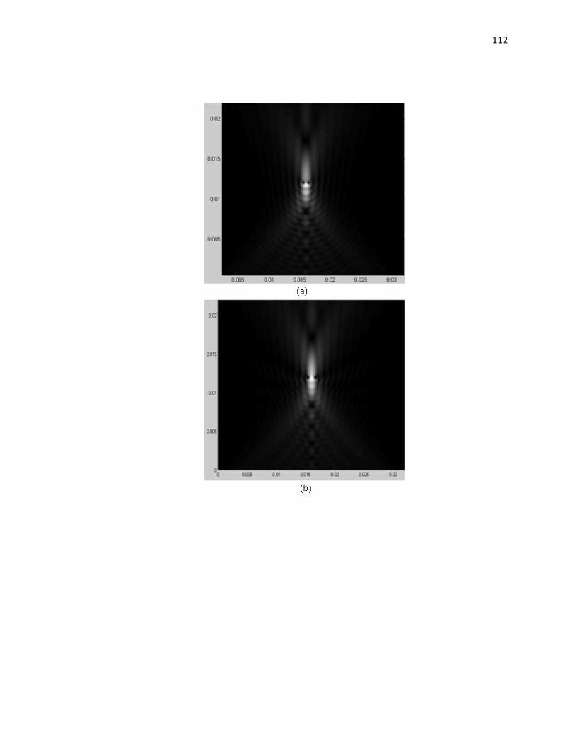
112

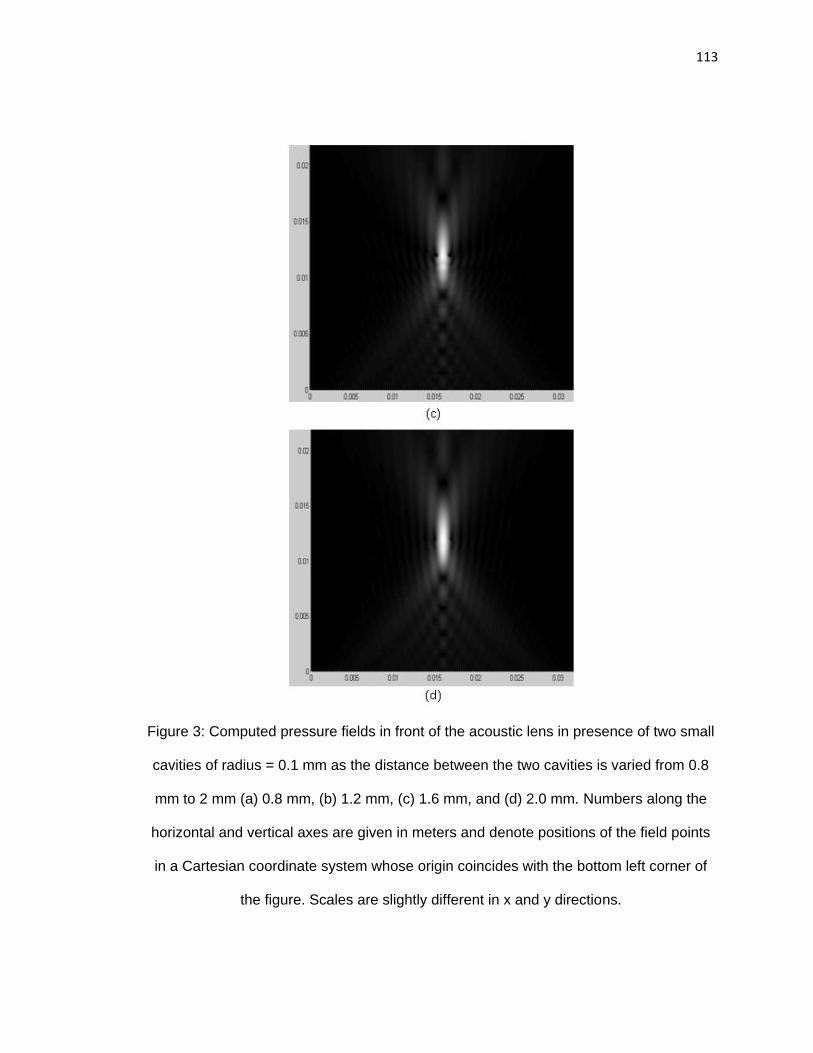
113

Figure 3: Computed pressure fields in front of the acoustic lens in presence of two small

cavities of radius = 0.1 mm as the distance between the two cavities is varied from 0.8

mm to 2 mm (a) 0.8 mm, (b) 1.2 mm, (c) 1.6 mm, and (d) 2.0 mm. Numbers along the

horizontal and vertical axes are given in meters and denote positions of the field points

in a Cartesian coordinate system whose origin coincides with the bottom left corner of

the figure. Scales are slightly different in x and y directions.

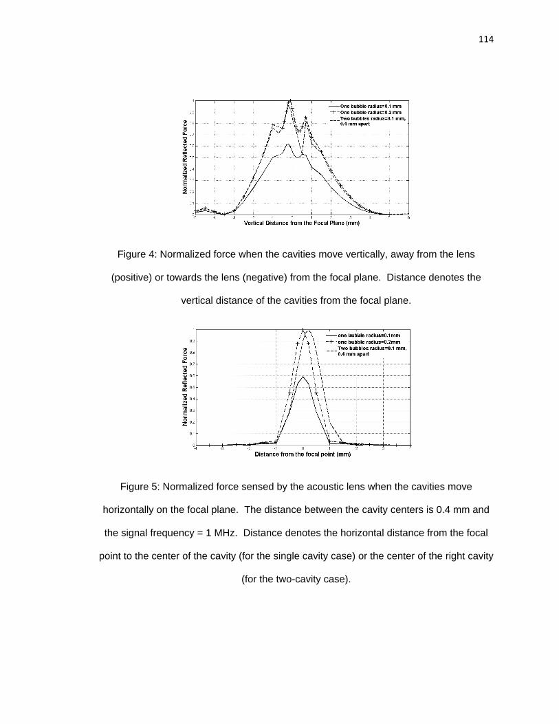
114

Figure 4: Normalized force when the cavities move vertically, away from the lens

(positive) or towards the lens (negative) from the focal plane. Distance denotes the

vertical distance of the cavities from the focal plane.

Figure 5: Normalized force sensed by the acoustic lens when the cavities move

horizontally on the focal plane. The distance between the cavity centers is 0.4 mm and

the signal frequency = 1 MHz. Distance denotes the horizontal distance from the focal

point to the center of the cavity (for the single cavity case) or the center of the right cavity

(for the two-cavity case).

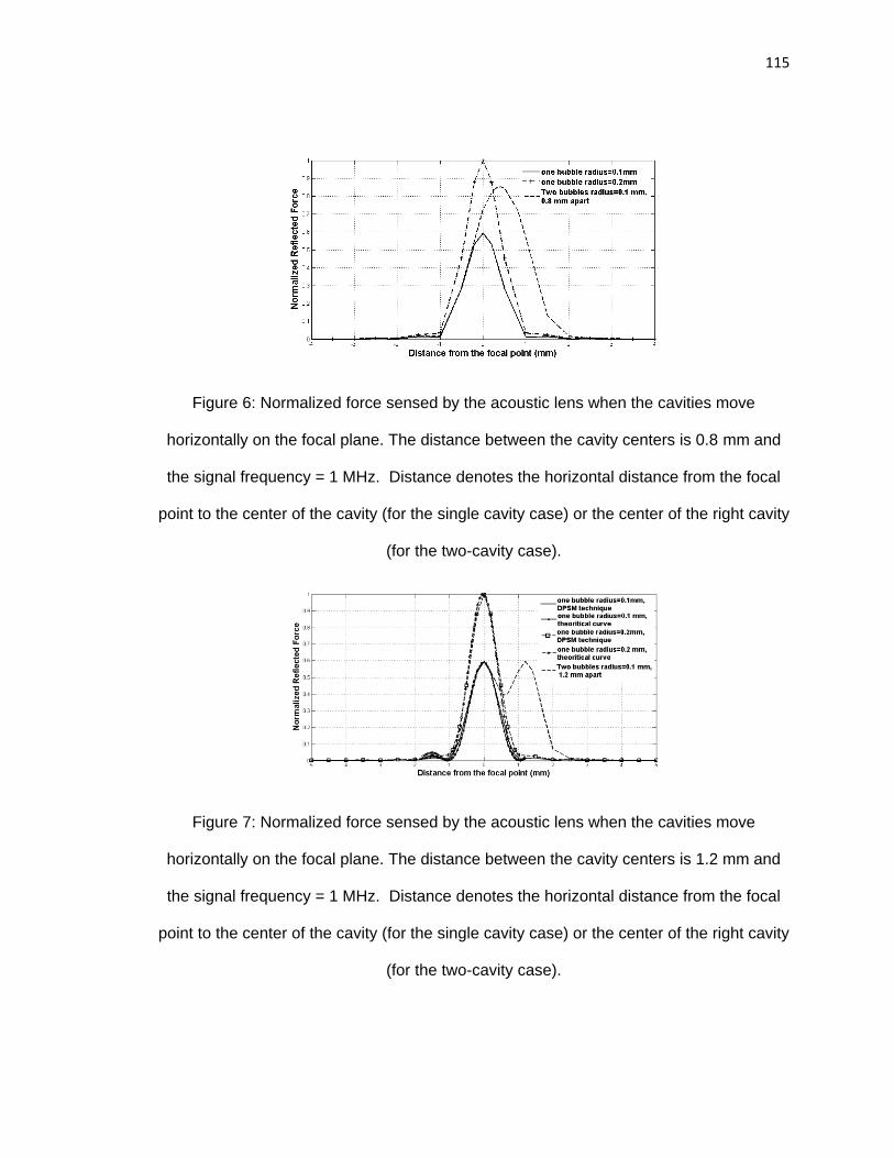
115

Figure 6: Normalized force sensed by the acoustic lens when the cavities move

horizontally on the focal plane. The distance between the cavity centers is 0.8 mm and

the signal frequency = 1 MHz. Distance denotes the horizontal distance from the focal

point to the center of the cavity (for the single cavity case) or the center of the right cavity

(for the two-cavity case).

Figure 7: Normalized force sensed by the acoustic lens when the cavities move

horizontally on the focal plane. The distance between the cavity centers is 1.2 mm and

the signal frequency = 1 MHz. Distance denotes the horizontal distance from the focal

point to the center of the cavity (for the single cavity case) or the center of the right cavity

(for the two-cavity case).

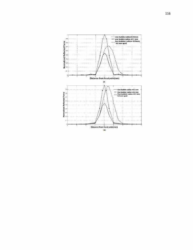
116

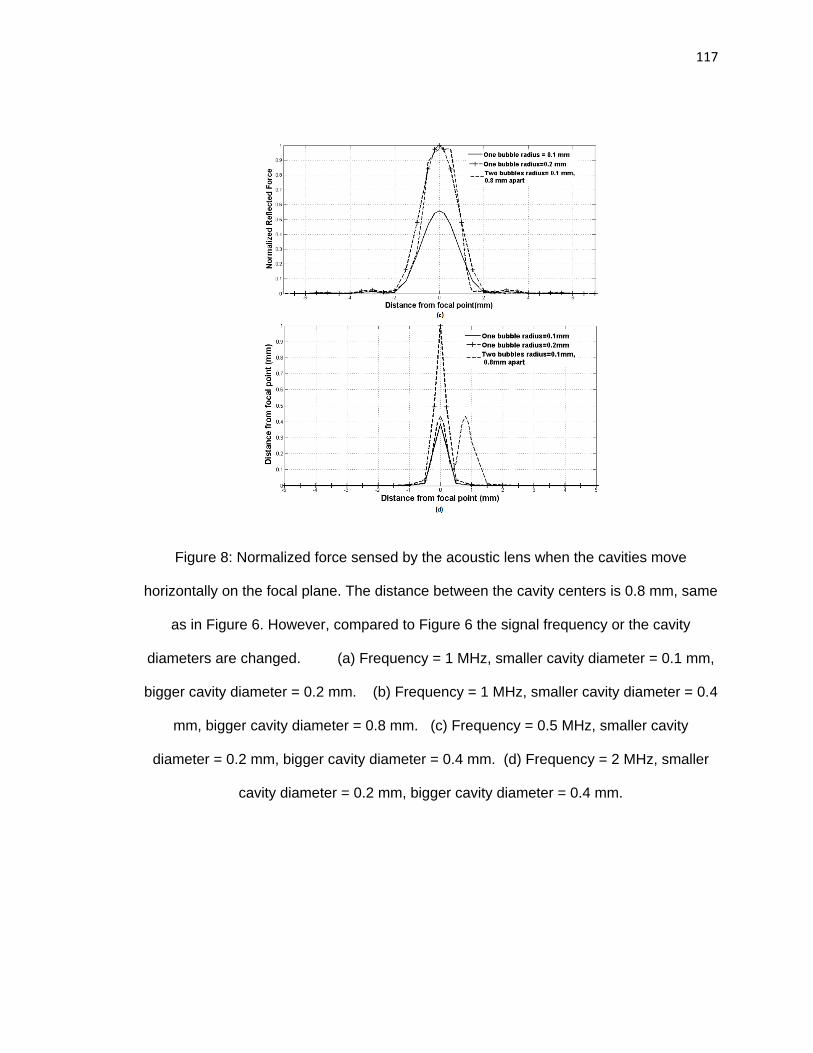
117

Figure 8: Normalized force sensed by the acoustic lens when the cavities move

horizontally on the focal plane. The distance between the cavity centers is 0.8 mm, same

as in Figure 6. However, compared to Figure 6 the signal frequency or the cavity

diameters are changed. (a) Frequency = 1 MHz, smaller cavity diameter = 0.1 mm,

bigger cavity diameter = 0.2 mm. (b) Frequency = 1 MHz, smaller cavity diameter = 0.4

mm, bigger cavity diameter = 0.8 mm. (c) Frequency = 0.5 MHz, smaller cavity

diameter = 0.2 mm, bigger cavity diameter = 0.4 mm. (d) Frequency = 2 MHz, smaller

cavity diameter = 0.2 mm, bigger cavity diameter = 0.4 mm.

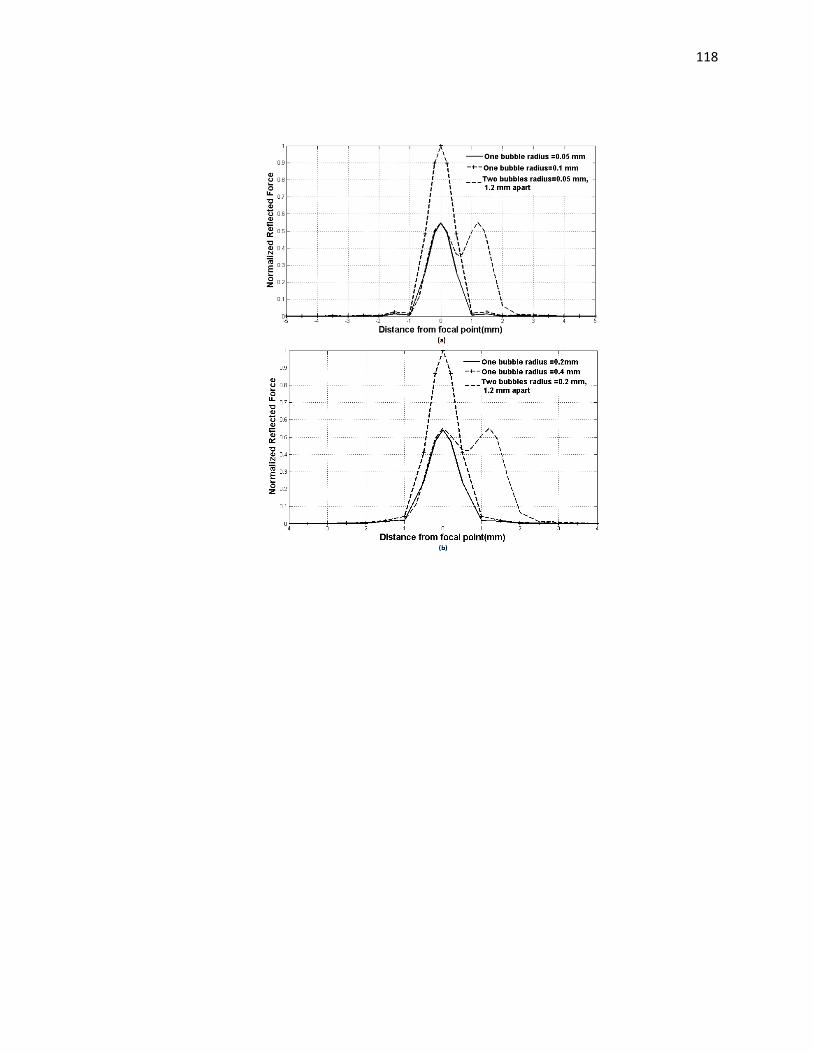
118

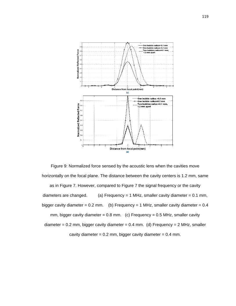
119

Figure 9: Normalized force sensed by the acoustic lens when the cavities move

horizontally on the focal plane. The distance between the cavity centers is 1.2 mm, same

as in Figure 7. However, compared to Figure 7 the signal frequency or the cavity

diameters are changed. (a) Frequency = 1 MHz, smaller cavity diameter = 0.1 mm,

bigger cavity diameter = 0.2 mm. (b) Frequency = 1 MHz, smaller cavity diameter = 0.4

mm, bigger cavity diameter = 0.8 mm. (c) Frequency = 0.5 MHz, smaller cavity

diameter = 0.2 mm, bigger cavity diameter = 0.4 mm. (d) Frequency = 2 MHz, smaller

cavity diameter = 0.2 mm, bigger cavity diameter = 0.4 mm.