Multidimensional spectral analysis of the ultrasonic radiofrequency

signal for characterization of media

Simona Granchi a, Enrico Vannacci a, Elena Biagi a,⇑, Leonardo Masotti b

aDepartment of Information Engineering (DINFO), University of Florence, via Santa Marta 3, 50139 Florence, Italyb El.En. S.p.A., Scientific Committee, Via Baldanzese 17, 50041 Calenzano, Florence, Italy

a r t i c l e i n f o

Article history:

Received 1 July 2015

Received in revised form 8 February 2016

Accepted 11 February 2016

Available online 16 February 2016

Keywords:

Ultrasonic radiofrequency signal

Spectral analysis

Signal processing

Tissue characterization

Quantitative ultrasound

a b s t r a c t

The importance of the analysis of the radiofrequency signal is by now recognized in the field of tissue

characterization via ultrasound. The RF signal contains a wealth of information and structural details that

are usually lost in the B-Mode representation. The HyperSPACE (Hyper SPectral Analysis for

Characterization in Echography) algorithm presented by the authors in previous papers for clinical appli-

cations is based on the radiofrequency ultrasonic signal. The present work describes the method in detail

and evaluates its performance in a repeatable and standardized manner, by using two test objects: a com-

mercial test object that simulates the human parenchyma, and a laboratory-made test object consisting

of human blood at different dilution values. In particular, the sensitivity and specificity in discriminating

different density levels were estimated. In addition, the robustness of the algorithm with respect to the

signal-to-noise ratio was also evaluated.

� 2016 The Authors. Published by Elsevier B.V. This is an open access article under the CC BY-NC-ND

license (http://creativecommons.org/licenses/by-nc-nd/4.0/).

1. Introduction

When an ultrasonic wave propagates through soft tissue, an

interaction occurs between the mechanical energy of the wave

and the local structure, generating energy absorption, reflection,

and scattering. The energy propagated back toward the ultrasonic

transducer constitutes the ultrasonic echo signal called the

radiofrequency (RF) signal. The RF signal contains information

about ultrasound–tissue interaction [1–8] and a processing

method must be used that is capable of extracting this information.

The amplitude is related to the distribution of mechanical impe-

dance (density, elastic characteristics) of the backscattering med-

ium, the scatterer concentration and the ratio between the sizes

of the microstructure and the wavelength [1,3,9,10]. The phase

information, related to the interferences, depends on the mutual

distances and geometrical organization of the tissue microstruc-

ture scatterers. These interferences and reflectivity variations in

the time domain are responsible for spectral amplitude modulation

in the frequency domain. In this context, over the last thirty years

quantitative ultrasound (QUS) techniques have been developed

[11–13] to improve tissue characterization as a support for

diagnostics. Indeed, in order to gain further information for tissue

characterization and differentiation purposes, it is essential not

only to preserve the shape of the RF signal spectrum, but also to

identify the spectral parameters that are best correlated with the

investigated structures [3,4,9,14–25].

Our group used the RF signal for our investigation techniques

[26,27] and developed the RULES (Radiofrequency Ultrasonic Local

EStimators) algorithm [28–32] based on the analysis of the local

power spectrum obtained by DWPT (Discrete Wavelet Transform).

Even though significant results have been achieved in various

research fields [23,27–29,33,34], they have been below expecta-

tions. In fact, the method was dependent on the instrumental

parameters of the acquisition setup [24,25] and the number of

extracted features was insufficient for characterizing tissue with

good specificity and sensitivity as demonstrated by the results

obtained by comparing the RULES with the method discussed in

this paper [35].

The proposed investigation method called HyperSPACE (Hyper

SPectral Analysis for Characterization in Echography) is able to

extract local information about the tissue under investigation

and implements a sub-band spectral decomposition. The method

in not directly based on the analysis of the power spectrum of

the RF signal, as with RULES and the principal QUS techniques,

however it works in a spectral domain of N-dimensions; this is

the origin of the Hyper suffix in the name, where N is the number

of sub-bands into which the RF signal bandwidth is decomposed.

http://dx.doi.org/10.1016/j.ultras.2016.02.010

0041-624X/� 2016 The Authors. Published by Elsevier B.V.

This is an open access article under the CC BY-NC-ND license (http://creativecommons.org/licenses/by-nc-nd/4.0/).

⇑ Corresponding author at: Ultrasound and Non-Destructive Testing Lab, Depart-

ment of Information Engineering (DINFO), University of Florence, via Santa Marta 3,

50139 Florence, Italy. Tel.: +39 055 2758606; fax: +39 055 2758570.

E-mail address: elena.biagi@unifi.it (E. Biagi).

Ultrasonics 68 (2016) 89–101

Contents lists available at ScienceDirect

Ultrasonics

journal homepage: www.elsevier .com/locate /ul t ras

Mor

e in

fo a

bout

this

art

icle

: ht

tp://

ww

w.n

dt.n

et/?

id=

1909

4

The method was applied in an important experimentation

involving ten Italian hospital clinics in order to differentiate the

two most common breast pathologies [35–37]. High values of sen-

sitivity and specificity in differentiating fibroadenoma and infil-

trating ductal carcinoma were obtained and compared with

histological examinations.

In previous works, we focused our attention on the training

phase of the algorithm and the description of the results. In the

present paper, the fundamental steps of the algorithm are

explained in detail. Moreover, the sensitivity of the method, the

dependence of the method on the instrumental parameters, and

the robustness of the algorithm with respect to the signal-to-

noise ratio (SNR) have been estimated. To do this, it was important

to test the method starting from the analysis of a single parameter

by using commercial and simple test objects. Two different test

objects were used. The first, a commercial CIRS model 047 (Com-

puterized Imaging Reference Systems, Inc. Norfolk, Virginia

23513 USA) test object, consists of background material that sim-

ulates the human parenchyma with a series of aggregates at differ-

ent densities inserted to simulate the presence of cysts. The second

was a laboratory test object consisting of a transfusion bag con-

taining human blood at different concentrations. Due to the char-

acteristics of the two test objects, density was chosen as the

parameter for evaluating the properties of the HyperSPACE

algorithm.

2. Investigation method

The proposed algorithm can be classified as a QUS technique

based on the analysis of the backscattered ultrasonic RF signal.

Moreover, it performs a sort of Texture Analysis [13,38–40] as it

tries to characterize the echographic image by extracting the typ-

ical features that determine the texture. In diagnostic ultrasounds,

texture analysis can be performed either directly by analyzing the

correlations among spatial gray-levels of B-Mode images, or indi-

rectly with QUS techniques applied to the spectral features. The

purpose of the algorithm is to identify a new spectral domain

where the signal parameters, correlated with the mechanical char-

acteristics and structural organization of the medium under inves-

tigation, can be extracted.

The investigation method works in a hyperspace consisting of N

spectral dimensions obtained from a sub-band decomposition of

the RF signal in order to read the local spectral amplitude modula-

tions generated by the distribution of the scatterers. Another speci-

fic characteristic of the method is the implementation of ‘‘local

normalization” that takes into account the effective energy of the

ultrasonic wave which insonifies the ‘‘local” portion of the med-

ium. In addition, the proposed normalization allows the algorithm

to be independent from the instrumental acquisition parameters of

the echographic scanner, such as Time Gain Compensation (TGC)

and transmission power.

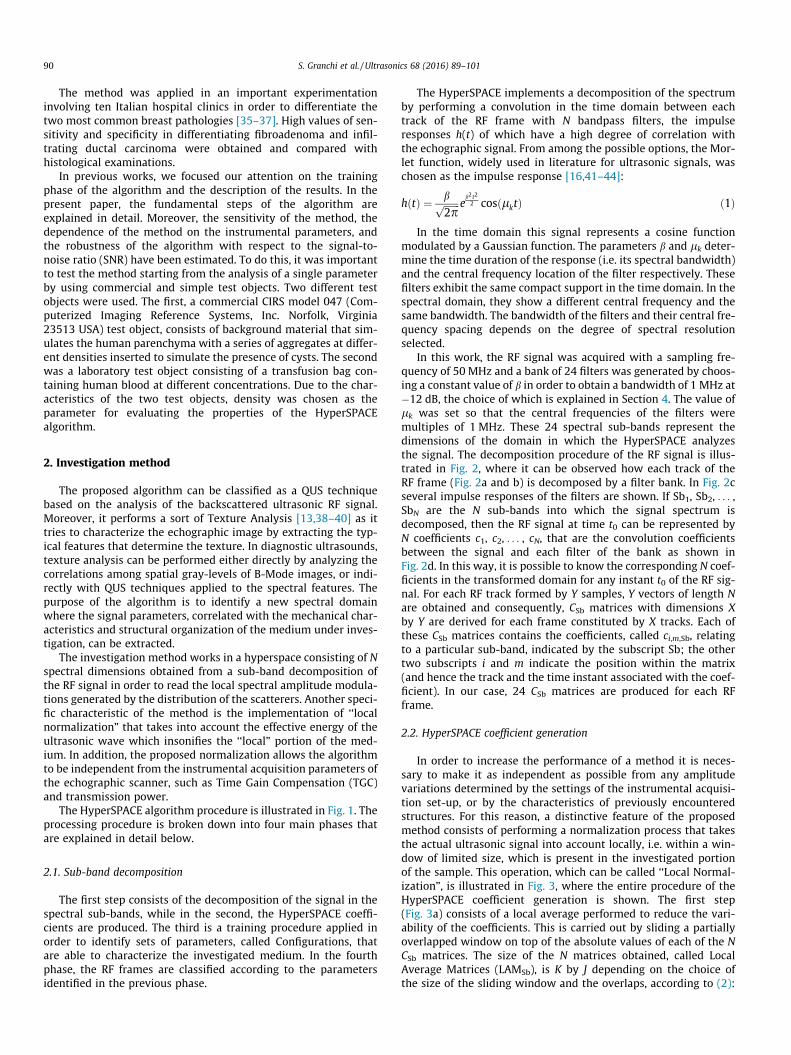
The HyperSPACE algorithm procedure is illustrated in Fig. 1. The

processing procedure is broken down into four main phases that

are explained in detail below.

2.1. Sub-band decomposition

The first step consists of the decomposition of the signal in the

spectral sub-bands, while in the second, the HyperSPACE coeffi-

cients are produced. The third is a training procedure applied in

order to identify sets of parameters, called Configurations, that

are able to characterize the investigated medium. In the fourth

phase, the RF frames are classified according to the parameters

identified in the previous phase.

The HyperSPACE implements a decomposition of the spectrum

by performing a convolution in the time domain between each

track of the RF frame with N bandpass filters, the impulse

responses h(t) of which have a high degree of correlation with

the echographic signal. From among the possible options, the Mor-

let function, widely used in literature for ultrasonic signals, was

chosen as the impulse response [16,41–44]:

hðtÞ ¼ bffiffiffiffiffiffiffi

2pp e

b2 t2

2 cosðlktÞ ð1Þ

In the time domain this signal represents a cosine function

modulated by a Gaussian function. The parameters b and lk deter-

mine the time duration of the response (i.e. its spectral bandwidth)

and the central frequency location of the filter respectively. These

filters exhibit the same compact support in the time domain. In the

spectral domain, they show a different central frequency and the

same bandwidth. The bandwidth of the filters and their central fre-

quency spacing depends on the degree of spectral resolution

selected.

In this work, the RF signal was acquired with a sampling fre-

quency of 50 MHz and a bank of 24 filters was generated by choos-

ing a constant value of b in order to obtain a bandwidth of 1 MHz at

�12 dB, the choice of which is explained in Section 4. The value of

lk was set so that the central frequencies of the filters were

multiples of 1 MHz. These 24 spectral sub-bands represent the

dimensions of the domain in which the HyperSPACE analyzes

the signal. The decomposition procedure of the RF signal is illus-

trated in Fig. 2, where it can be observed how each track of the

RF frame (Fig. 2a and b) is decomposed by a filter bank. In Fig. 2c

several impulse responses of the filters are shown. If Sb1, Sb2, . . . ,

SbN are the N sub-bands into which the signal spectrum is

decomposed, then the RF signal at time t0 can be represented by

N coefficients c1, c2, . . . , cN, that are the convolution coefficients

between the signal and each filter of the bank as shown in

Fig. 2d. In this way, it is possible to know the corresponding N coef-

ficients in the transformed domain for any instant t0 of the RF sig-

nal. For each RF track formed by Y samples, Y vectors of length N

are obtained and consequently, CSb matrices with dimensions X

by Y are derived for each frame constituted by X tracks. Each of

these CSb matrices contains the coefficients, called ci,m,Sb, relating

to a particular sub-band, indicated by the subscript Sb; the other

two subscripts i and m indicate the position within the matrix

(and hence the track and the time instant associated with the coef-

ficient). In our case, 24 CSb matrices are produced for each RF

frame.

2.2. HyperSPACE coefficient generation

In order to increase the performance of a method it is neces-

sary to make it as independent as possible from any amplitude

variations determined by the settings of the instrumental acquisi-

tion set-up, or by the characteristics of previously encountered

structures. For this reason, a distinctive feature of the proposed

method consists of performing a normalization process that takes

the actual ultrasonic signal into account locally, i.e. within a win-

dow of limited size, which is present in the investigated portion

of the sample. This operation, which can be called ‘‘Local Normal-

ization”, is illustrated in Fig. 3, where the entire procedure of the

HyperSPACE coefficient generation is shown. The first step

(Fig. 3a) consists of a local average performed to reduce the vari-

ability of the coefficients. This is carried out by sliding a partially

overlapped window on top of the absolute values of each of the N

CSb matrices. The size of the N matrices obtained, called Local

Average Matrices (LAMSb), is K by J depending on the choice of

the size of the sliding window and the overlaps, according to (2):

90 S. Granchi et al. / Ultrasonics 68 (2016) 89–101

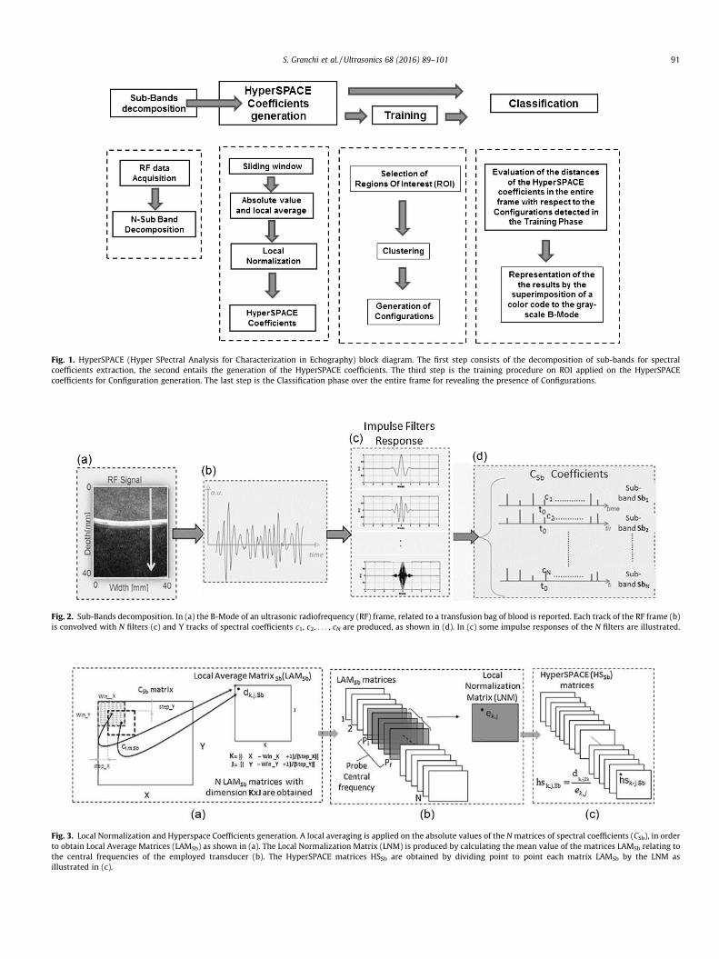
Fig. 1. HyperSPACE (Hyper SPectral Analysis for Characterization in Echography) block diagram. The first step consists of the decomposition of sub-bands for spectral

coefficients extraction, the second entails the generation of the HyperSPACE coefficients. The third step is the training procedure on ROI applied on the HyperSPACE

coefficients for Configuration generation. The last step is the Classification phase over the entire frame for revealing the presence of Configurations.

Fig. 2. Sub-Bands decomposition. In (a) the B-Mode of an ultrasonic radiofrequency (RF) frame, related to a transfusion bag of blood is reported. Each track of the RF frame (b)

is convolved with N filters (c) and Y tracks of spectral coefficients c1, c2, . . . , cN are produced, as shown in (d). In (c) some impulse responses of the N filters are illustrated.

Fig. 3. Local Normalization and Hyperspace Coefficients generation. A local averaging is applied on the absolute values of the Nmatrices of spectral coefficients (CSb), in order

to obtain Local Average Matrices (LAMSb) as shown in (a). The Local Normalization Matrix (LNM) is produced by calculating the mean value of the matrices LAMSb relating to

the central frequencies of the employed transducer (b). The HyperSPACE matrices HSSb are obtained by dividing point to point each matrix LAMSb by the LNM as

illustrated in (c).

S. Granchi et al. / Ultrasonics 68 (2016) 89–101 91

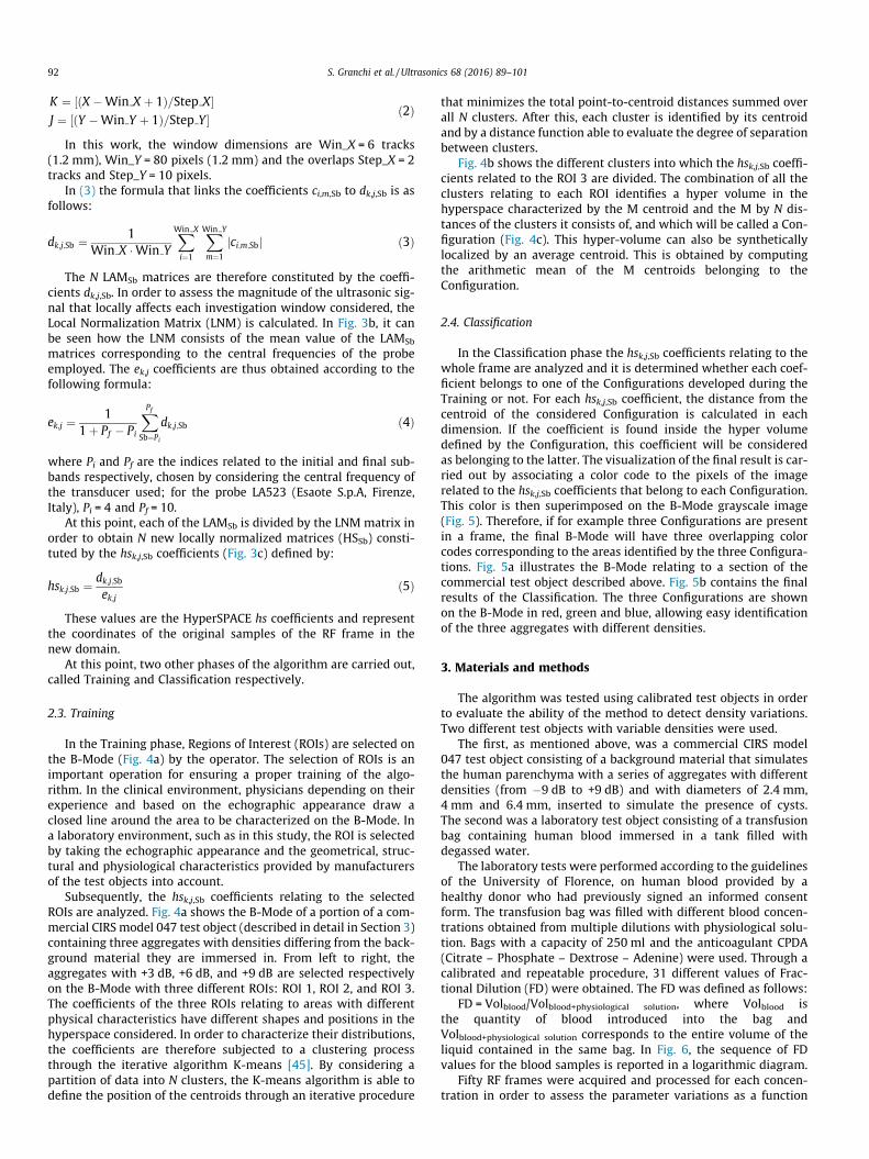
K ¼ ½ðX �Win X þ 1Þ=Step X�J ¼ ½ðY �Win Y þ 1Þ=Step Y� ð2Þ

In this work, the window dimensions are Win_X = 6 tracks

(1.2 mm), Win_Y = 80 pixels (1.2 mm) and the overlaps Step_X = 2

tracks and Step_Y = 10 pixels.

In (3) the formula that links the coefficients ci,m,Sb to dk,j,Sb is as

follows:

dk;j;Sb ¼ 1

Win X �Win Y

X

Win X

i¼1

X

Win Y

m¼1

jci;m;Sbj ð3Þ

The N LAMSb matrices are therefore constituted by the coeffi-

cients dk,j,Sb. In order to assess the magnitude of the ultrasonic sig-

nal that locally affects each investigation window considered, the

Local Normalization Matrix (LNM) is calculated. In Fig. 3b, it can

be seen how the LNM consists of the mean value of the LAMSb

matrices corresponding to the central frequencies of the probe

employed. The ek,j coefficients are thus obtained according to the

following formula:

ek;j ¼1

1þ Pf � Pi

X

Pf

Sb¼Pi

dk;j;Sb ð4Þ

where Pi and Pf are the indices related to the initial and final sub-

bands respectively, chosen by considering the central frequency of

the transducer used; for the probe LA523 (Esaote S.p.A, Firenze,

Italy), Pi = 4 and Pf = 10.

At this point, each of the LAMSb is divided by the LNM matrix in

order to obtain N new locally normalized matrices (HSSb) consti-

tuted by the hsk,j,Sb coefficients (Fig. 3c) defined by:

hsk;j;Sb ¼ dk;j;Sb

ek;jð5Þ

These values are the HyperSPACE hs coefficients and represent

the coordinates of the original samples of the RF frame in the

new domain.

At this point, two other phases of the algorithm are carried out,

called Training and Classification respectively.

2.3. Training

In the Training phase, Regions of Interest (ROIs) are selected on

the B-Mode (Fig. 4a) by the operator. The selection of ROIs is an

important operation for ensuring a proper training of the algo-

rithm. In the clinical environment, physicians depending on their

experience and based on the echographic appearance draw a

closed line around the area to be characterized on the B-Mode. In

a laboratory environment, such as in this study, the ROI is selected

by taking the echographic appearance and the geometrical, struc-

tural and physiological characteristics provided by manufacturers

of the test objects into account.

Subsequently, the hsk,j,Sb coefficients relating to the selected

ROIs are analyzed. Fig. 4a shows the B-Mode of a portion of a com-

mercial CIRS model 047 test object (described in detail in Section 3)

containing three aggregates with densities differing from the back-

ground material they are immersed in. From left to right, the

aggregates with +3 dB, +6 dB, and +9 dB are selected respectively

on the B-Mode with three different ROIs: ROI 1, ROI 2, and ROI 3.

The coefficients of the three ROIs relating to areas with different

physical characteristics have different shapes and positions in the

hyperspace considered. In order to characterize their distributions,

the coefficients are therefore subjected to a clustering process

through the iterative algorithm K-means [45]. By considering a

partition of data into N clusters, the K-means algorithm is able to

define the position of the centroids through an iterative procedure

that minimizes the total point-to-centroid distances summed over

all N clusters. After this, each cluster is identified by its centroid

and by a distance function able to evaluate the degree of separation

between clusters.

Fig. 4b shows the different clusters into which the hsk,j,Sb coeffi-

cients related to the ROI 3 are divided. The combination of all the

clusters relating to each ROI identifies a hyper volume in the

hyperspace characterized by the M centroid and the M by N dis-

tances of the clusters it consists of, and which will be called a Con-

figuration (Fig. 4c). This hyper-volume can also be synthetically

localized by an average centroid. This is obtained by computing

the arithmetic mean of the M centroids belonging to the

Configuration.

2.4. Classification

In the Classification phase the hsk,j,Sb coefficients relating to the

whole frame are analyzed and it is determined whether each coef-

ficient belongs to one of the Configurations developed during the

Training or not. For each hsk,j,Sb coefficient, the distance from the

centroid of the considered Configuration is calculated in each

dimension. If the coefficient is found inside the hyper volume

defined by the Configuration, this coefficient will be considered

as belonging to the latter. The visualization of the final result is car-

ried out by associating a color code to the pixels of the image

related to the hsk,j,Sb coefficients that belong to each Configuration.

This color is then superimposed on the B-Mode grayscale image

(Fig. 5). Therefore, if for example three Configurations are present

in a frame, the final B-Mode will have three overlapping color

codes corresponding to the areas identified by the three Configura-

tions. Fig. 5a illustrates the B-Mode relating to a section of the

commercial test object described above. Fig. 5b contains the final

results of the Classification. The three Configurations are shown

on the B-Mode in red, green and blue, allowing easy identification

of the three aggregates with different densities.

3. Materials and methods

The algorithm was tested using calibrated test objects in order

to evaluate the ability of the method to detect density variations.

Two different test objects with variable densities were used.

The first, as mentioned above, was a commercial CIRS model

047 test object consisting of a background material that simulates

the human parenchyma with a series of aggregates with different

densities (from �9 dB to +9 dB) and with diameters of 2.4 mm,

4 mm and 6.4 mm, inserted to simulate the presence of cysts.

The second was a laboratory test object consisting of a transfusion

bag containing human blood immersed in a tank filled with

degassed water.

The laboratory tests were performed according to the guidelines

of the University of Florence, on human blood provided by a

healthy donor who had previously signed an informed consent

form. The transfusion bag was filled with different blood concen-

trations obtained from multiple dilutions with physiological solu-

tion. Bags with a capacity of 250 ml and the anticoagulant CPDA

(Citrate – Phosphate – Dextrose – Adenine) were used. Through a

calibrated and repeatable procedure, 31 different values of Frac-

tional Dilution (FD) were obtained. The FD was defined as follows:

FD = Volblood/Volblood+physiological solution, where Volblood is

the quantity of blood introduced into the bag and

Volblood+physiological solution corresponds to the entire volume of the

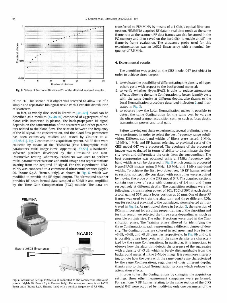
liquid contained in the same bag. In Fig. 6, the sequence of FD

values for the blood samples is reported in a logarithmic diagram.

Fifty RF frames were acquired and processed for each concen-

tration in order to assess the parameter variations as a function

92 S. Granchi et al. / Ultrasonics 68 (2016) 89–101

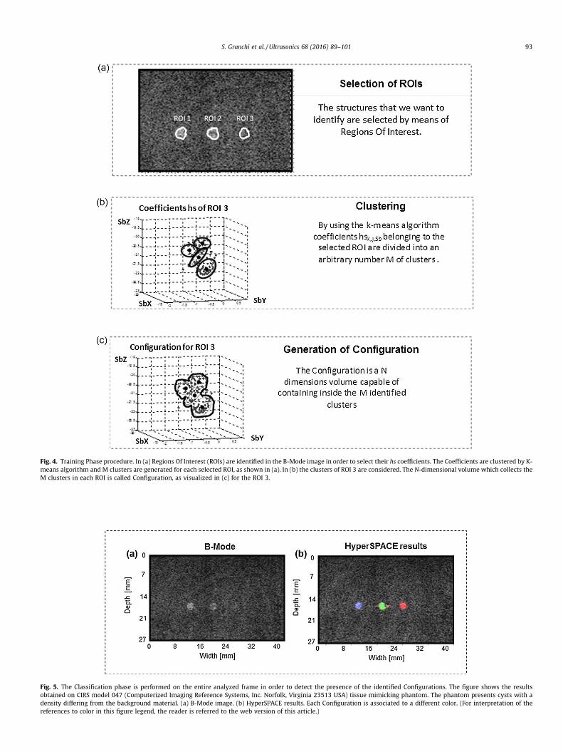
Fig. 4. Training Phase procedure. In (a) Regions Of Interest (ROIs) are identified in the B-Mode image in order to select their hs coefficients. The Coefficients are clustered by K-

means algorithm and M clusters are generated for each selected ROI, as shown in (a). In (b) the clusters of ROI 3 are considered. The N-dimensional volume which collects the

M clusters in each ROI is called Configuration, as visualized in (c) for the ROI 3.

Fig. 5. The Classification phase is performed on the entire analyzed frame in order to detect the presence of the identified Configurations. The figure shows the results

obtained on CIRS model 047 (Computerized Imaging Reference Systems, Inc. Norfolk, Virginia 23513 USA) tissue mimicking phantom. The phantom presents cysts with a

density differing from the background material. (a) B-Mode image. (b) HyperSPACE results. Each Configuration is associated to a different color. (For interpretation of the

references to color in this figure legend, the reader is referred to the web version of this article.)

S. Granchi et al. / Ultrasonics 68 (2016) 89–101 93

of the FD. This second test object was selected to allow use of a

simple and repeatable biological tissue with a variable distribution

of scatterers.

In fact, as widely discussed in literature [46–49], blood can be

described as a medium [47,48,50] composed of aggregates of red

blood cells immersed in plasma. The back-propagated RF signal

depends on the concentration of the scatterers and other parame-

ters related to the blood flow. The relation between the frequency

of the RF signal, the concentration, and the blood flow parameters

has been extensively studied and tested by Cloutier et al.

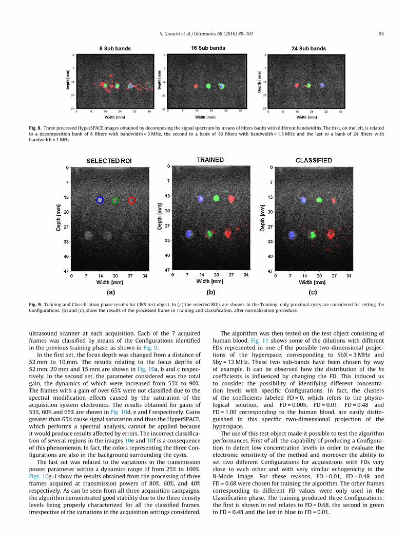
[47,48,51]. Fig. 7 contains the acquisition system. All RF data were

collected by means of the FEMMINA (Fast Echographic Multi

parameters Multi Image Novel Apparatus) [52,53], a hardware-

software platform developed by the Ultrasound and Non-

Destructive Testing Laboratory. FEMMINA was used to perform

multi-parameter extractions and multi-image data representations

starting from the acquired RF signal. For this experiment, FEM-

MINA was connected to a commercial ultrasound scanner (Mylab

90, Esaote S.p.A, Firenze, Italy), as shown in Fig. 6, which was

modified to provide the RF signal output. The ultrasound scanner

provides RF beam-formed data sampled at 50 MHz and amplified

by the Time Gain Compensation (TGC) module. The data are

transferred to FEMMINA by means of a 1 Gbit/s optical fiber con-

nection. FEMMINA acquires RF data in real time mode at the same

frame rate as the scanner. RF data frames can also be stored in the

PC memory and then saved on the hard disk to enable an off-line

frame-by-frame evaluation. The ultrasonic probe used for this

experimentation was an LA523 linear array with a nominal fre-

quency of 7.5 MHz.

4. Experimental results

The algorithm was tested on the CIRS model 047 test object in

order to achieve three targets:

1. to evaluate the possibility of differentiating the density of hyper

echoic cysts with respect to the background material;

2. to verify whether HyperSPACE is able to reduce attenuation

effects, allowing the same Configuration to better identify cysts

with the same density at different depths, also thanks to the

Local Normalization procedure described in Section 2 and illus-

trated in Fig. 3;

3. to observe how the Local Normalization makes it possible to

detect the same Configuration for the same cyst by varying

the ultrasound scanner acquisition settings such as focus depth,

transmission power, and total gain.

Before carrying out these experiments, several preliminary tests

were performed in order to select the best frequency range subdi-

vision. Different sub-band widths of filters were tested: 3 MHz,

1.5 MHz, 1 MHz and RF frames referring to proximal cysts of the

CIRS model 047 were processed. The goodness of the processed

images was evaluated in terms of ability to discriminate the den-

sity levels and differentiate the cysts from the surroundings. The

best compromise was obtained using a 1 MHz frequency sub-

band width, as can be observed in Fig. 8 which contains processed

HyperSPACE images using 3 MHz, 1.5 MHz and 1 MHz sub-band

widths. To achieve the first two objectives, 10 RF frames related

to sections not spatially correlated with each other were acquired

by moving the probe on the CIRS model 047. The acquired sections

contain two rows of cysts with diameters of 2.4 mm and 4 mm

respectively at different depths. The acquisition settings were the

following: a transmission power of 80%, TGC of 50% at each depth,

a total gain of 55%, and a focus position at 20 mm. One of these RF

frames was used to train the algorithm and three different ROIs,

one for each cyst proximal to the transducer, were selected as illus-

trated in Fig. 9a. As mentioned above in Section 2, the selection of

ROIs is important for ensuring proper training of the algorithm and

for this reason we selected the three cysts depending as much as

possible on their size. The other 9 sections were used in the Clas-

sification phase. The Training phase allowed for identifying the

three Configurations, each representing a different degree of den-

sity. The Configurations are colored in red, green and blue for the

+3 dB, +6 dB, and +9 dB densities respectively. In Fig. 9b and c, it

is possible to see how cysts with the same density are character-

ized by the same Configurations. In particular, it is important to

observe how the algorithm detects the presence of the aggregates

with a density of +3 dB, which is barely distinguishable from the

backgroundmaterial in the B-Mode image. It is even more interest-

ing to note how the cysts with the same density are characterized

by the same Configurations, regardless of their different depths,

thanks also to the Local Normalization process which reduces the

attenuation effects.

In order to test the Configurations by changing the acquisition

settings, three other measurement campaigns were performed.

For each one, 7 RF frames relating to the same section of the CIRS

model 047 were acquired by modifying only one parameter of the

Fig. 7. Acquisition set-up. FEMMINA is connected to the commercial ultrasound

scanner Mylab 90 (Esaote S.p.A, Firenze, Italy). The ultrasonic probe is an LA523

linear array (Esaote S.p.A, Firenze, Italy) with a nominal frequency of 7.5 MHz.

Fig. 6. Values of Fractional Dilutions (FD) of the all blood analyzed samples.

94 S. Granchi et al. / Ultrasonics 68 (2016) 89–101

ultrasound scanner at each acquisition. Each of the 7 acquired

frames was classified by means of the Configurations identified

in the previous training phase, as shown in Fig. 9.

In the first set, the focus depth was changed from a distance of

52 mm to 10 mm. The results relating to the focus depths of

52 mm, 20 mm and 15 mm are shown in Fig. 10a, b and c respec-

tively. In the second set, the parameter considered was the total

gain, the dynamics of which were increased from 55% to 90%.

The frames with a gain of over 65% were not classified due to the

spectral modification effects caused by the saturation of the

acquisition system electronics. The results obtained for gains of

55%, 60% and 65% are shown in Fig. 10d, e and f respectively. Gains

greater than 65% cause signal saturation and thus the HyperSPACE,

which performs a spectral analysis, cannot be applied because

it would produce results affected by errors. The incorrect classifica-

tion of several regions in the images 10e and 10f is a consequence

of this phenomenon. In fact, the colors representing the three Con-

figurations are also in the background surrounding the cysts.

The last set was related to the variations in the transmission

power parameter within a dynamics range of from 25% to 100%.

Figs. 10g–i show the results obtained from the processing of three

frames acquired at transmission powers of 80%, 60%, and 40%

respectively. As can be seen from all three acquisition campaigns,

the algorithm demonstrated good stability due to the three density

levels being properly characterized for all the classified frames,

irrespective of the variations in the acquisition settings considered.

The algorithm was then tested on the test object consisting of

human blood. Fig. 11 shows some of the dilutions with different

FDs represented in one of the possible two-dimensional projec-

tions of the hyperspace, corresponding to SbX = 3 MHz and

Sby = 13 MHz. These two sub-bands have been chosen by way

of example. It can be observed how the distribution of the hs

coefficients is influenced by changing the FD. This induced us

to consider the possibility of identifying different concentra-

tion levels with specific Configurations. In fact, the clusters

of the coefficients labeled FD = 0, which refers to the physio-

logical solution, and FD = 0.005, FD = 0.01, FD = 0.48 and

FD = 1.00 corresponding to the human blood, are easily distin-

guished in this specific two-dimensional projection of the

hyperspace.

The use of this test object made it possible to test the algorithm

performances. First of all, the capability of producing a Configura-

tion to detect low concentration levels in order to evaluate the

electronic sensitivity of the method and moreover the ability to

set two different Configurations for acquisitions with FDs very

close to each other and with very similar echogenicity in the

B-Mode image. For these reasons, FD = 0.01, FD = 0.48 and

FD = 0.68 were chosen for training the algorithm. The other frames

corresponding to different FD values were only used in the

Classification phase. The training produced three Configurations:

the first is shown in red relates to FD = 0.68, the second in green

to FD = 0.48 and the last in blue to FD = 0.01.

Fig. 9. Training and Classification phase results for CIRS test object. In (a) the selected ROIs are shown. In the Training, only proximal cysts are considered for setting the

Configurations. (b) and (c), show the results of the processed frame in Training and Classification, after normalization procedure.

Fig. 8. Three processed HyperSPACE images obtained by decomposing the signal spectrum by means of filters banks with different bandwidths. The first, on the left, is related

to a decomposition bank of 8 filters with bandwidth = 3 MHz, the second to a bank of 16 filters with bandwidth = 1.5 MHz and the last to a bank of 24 filters with

bandwidth = 1 MHz.

S. Granchi et al. / Ultrasonics 68 (2016) 89–101 95

The average values of the gray levels calculated within a win-

dow inside the blood bag for each of the 31 dilutions are reported

in Fig. 12. It is worth noting, for example, how the frames with

FD = 0.48 and FD = 0.68 show very similar gray-level values.

Fig. 13 contains the colored area percentages relating to the three

Configurations produced in the training phase. The percentages

were estimated on each of the 31 frames, with respect to the entire

frame in order to take into account the capability of each Configu-

ration both to characterize only one specific FD value and not to

mark areas outside the bag blood, as represented in the B-Mode

of Figs. 12 and 14 by the regions below the strong reflection. A

good degree of selectivity for the Configurations relating to

FD = 0.48 (green), and FD = 0.68 (red) can be observed, as they

are minimally superimposed. Fig. 14 contains nine processed

images relating to different dilutions. In addition to the three

frames used in the training phase, several frames subjected to

the classification phase only are also reported. Also in this case,

as confirmed by Fig. 13, it is possible to observe how the three

Configurations seem to be very selective, i.e. the colored areas on

the classified frames are either very small or absent. In Fig. 14 it

is evident that the two green and red Configurations, in addition

to differing one from the other, do not appear in the frames with

dilutions close to FD = 0.48 or FD = 0.68. It can also be observed

how the frames used for the training phase are not uniformly colored,

due to the inevitable formation of aggregation centers [47].

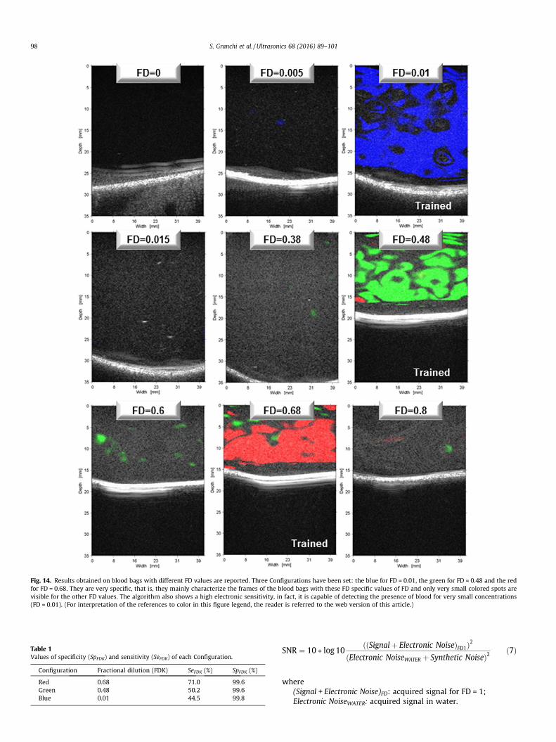
In order to calculate the specificity (SpFDK) and sensitivity (SeFDK)

of each Configuration, the following expressions were applied [54]:

SeFDK ¼ TPFDK

TPFDK þ FNFDK

SpFDK ¼ TNFDK

TNFDK þ FPFDK

ð6Þ

Fig. 10. In (a–c) Classification results obtained at variable focus depths. In (d–f) Classification results obtained for different gains and in (g–i) Classification results obtained for

different transmission powers. The analyzed sections contain two rows of cysts with diameters of 2.4 mm (proximal) and 4 mm (at a greater depth).

96 S. Granchi et al. / Ultrasonics 68 (2016) 89–101

where

TPFDK: area of regions into blood bags with FD ¼ FDK truly

stained by Configuration for FD ¼ FDK;

FNFDK: area of regions into blood bags with FD ¼ FDK falsely not

stained by Configurations for FD ¼ FDK;

FPFDK: area of regions into blood bags with FD– FDK falsely

stained by Configuration for FD ¼ FDK;

TNFDK: area of regions into blood bags with FD– FDK truly not

stained by Configurations for FD ¼ FDK.

Estimated values for the defined Configurations are reported in

Table 1.

The obtained values are due to the choice of having trained the

method favoring the specificity with respect to sensitivity. Actually,

in many cases the clinical diagnosis is concerned, not only to detect

the presence of disease, but especially to differentiate its nature from

other types of pathologies with high level of safety. Another consid-

eration needs to be made about SeFDK, that, according to the defini-

tion of TPFDK and FNFDK, resulted to be affected by the non

homogeneous FD distribution into the blood bags, as said above.

Moreover, the minimum FD level detectable by the BLUE Con-

figuration was FD = 0.01 and represent the electronic sensitivity

of HyperSPACE method. In fact, it was decided to set a Configura-

tion for FD = 0.005, however, FD = 0 was also marked in the Classi-

fication, demonstrating that noise and no blood was detected.

It must be pointed out that to assess the stability of a processing

method, it is necessary to evaluate its performance as a function of

the signal-to-noise (SNR) ratio. In order to achieve this for the

HyperSPACE, the acquisition with FD equal to 1 is considered.

Moreover, an acquisition was performed with the transducer

immersed in water with identical parameters to those used in

the acquisition with FD = 1. Different values of synthetic coherent

noise created in the Matlab environment (MathWorks, Natick,

Massachusetts, USA) were added to this acquisition to obtain 32

different frames with increasing noise. The synthetic noise was fil-

tered by the frequency response of the probe used. On each of

these frames, the same ROI was selected in the focalized region

and the noise was calculated for the 32 different values of the

added synthetic noise, according to the formula:

Fig. 12. Gray level mean value calculated on the B-Mode images, in relation to different FD values. For FD from 0.25 up to 0.9, the gray level mean has small fluctuations and

therefore it is very difficult to distinguish the different dilution levels through the analysis of the B-Mode images.

Fig. 13. Percentage of Colored Area calculated on every frame with different FD

depending on the FD values. The percentage is calculated for the entire frame. It can

be noted how the three colors have very low superimpositions for different FD

values and are very specific for the FD selected for the training.

Fig. 11. Example of coefficients hs at different FD values is shown in a two-

dimensional projection of the N dimension hyperspace. The choice of these sub-

bands in the figure is only to give an example. It is worth noting that different

clusters correspond to different FD values.

S. Granchi et al. / Ultrasonics 68 (2016) 89–101 97

SNR ¼ 10 � log 10 ððSignalþ Electronic NoiseÞFD1Þ2

ðElectronic NoiseWATER þ Synthetic NoiseÞ2ð7Þ

where

(Signal + Electronic Noise)FD: acquired signal for FD = 1;

Electronic NoiseWATER: acquired signal in water.

Fig. 14. Results obtained on blood bags with different FD values are reported. Three Configurations have been set: the blue for FD = 0.01, the green for FD = 0.48 and the red

for FD = 0.68. They are very specific, that is, they mainly characterize the frames of the blood bags with these FD specific values of FD and only very small colored spots are

visible for the other FD values. The algorithm also shows a high electronic sensitivity, in fact, it is capable of detecting the presence of blood for very small concentrations

(FD = 0.01). (For interpretation of the references to color in this figure legend, the reader is referred to the web version of this article.)

Table 1

Values of specificity (SpFDK) and sensitivity (SeFDK) of each Configuration.

Configuration Fractional dilution (FDK) SeFDK (%) SpFDK (%)

Red 0.68 71.0 99.6

Green 0.48 50.2 99.6

Blue 0.01 44.5 99.8

98 S. Granchi et al. / Ultrasonics 68 (2016) 89–101

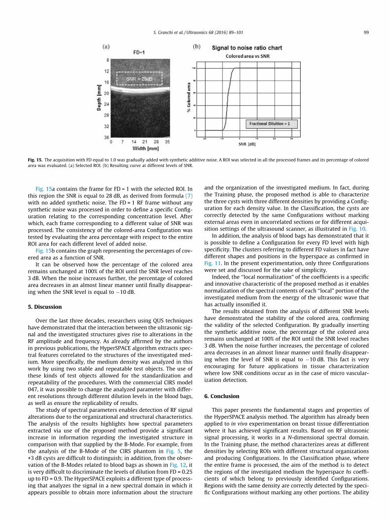
Fig. 15a contains the frame for FD = 1 with the selected ROI. In

this region the SNR is equal to 28 dB, as derived from formula (7)

with no added synthetic noise. The FD = 1 RF frame without any

synthetic noise was processed in order to define a specific Config-

uration relating to the corresponding concentration level. After

which, each frame corresponding to a different value of SNR was

processed. The consistency of the colored-area Configuration was

tested by evaluating the area percentage with respect to the entire

ROI area for each different level of added noise.

Fig. 15b contains the graph representing the percentages of cov-

ered area as a function of SNR.

It can be observed how the percentage of the colored area

remains unchanged at 100% of the ROI until the SNR level reaches

3 dB. When the noise increases further, the percentage of colored

area decreases in an almost linear manner until finally disappear-

ing when the SNR level is equal to �10 dB.

5. Discussion

Over the last three decades, researchers using QUS techniques

have demonstrated that the interaction between the ultrasonic sig-

nal and the investigated structures gives rise to alterations in the

RF amplitude and frequency. As already affirmed by the authors

in previous publications, the HyperSPACE algorithm extracts spec-

tral features correlated to the structures of the investigated med-

ium. More specifically, the medium density was analyzed in this

work by using two stable and repeatable test objects. The use of

these kinds of test objects allowed for the standardization and

repeatability of the procedures. With the commercial CIRS model

047, it was possible to change the analyzed parameter with differ-

ent resolutions through different dilution levels in the blood bags,

as well as ensure the replicability of results.

The study of spectral parameters enables detection of RF signal

alterations due to the organizational and structural characteristics.

The analysis of the results highlights how spectral parameters

extracted via use of the proposed method provide a significant

increase in information regarding the investigated structure in

comparison with that supplied by the B-Mode. For example, from

the analysis of the B-Mode of the CIRS phantom in Fig. 5, the

+3 dB cysts are difficult to distinguish; in addition, from the obser-

vation of the B-Modes related to blood bags as shown in Fig. 12, it

is very difficult to discriminate the levels of dilution from FD = 0.25

up to FD = 0.9. The HyperSPACE exploits a different type of process-

ing that analyzes the signal in a new spectral domain in which it

appears possible to obtain more information about the structure

and the organization of the investigated medium. In fact, during

the Training phase, the proposed method is able to characterize

the three cysts with three different densities by providing a Config-

uration for each density value. In the Classification, the cysts are

correctly detected by the same Configurations without marking

external areas even in uncorrelated sections or for different acqui-

sition settings of the ultrasound scanner, as illustrated in Fig. 10.

In addition, the analysis of blood bags has demonstrated that it

is possible to define a Configuration for every FD level with high

specificity. The clusters referring to different FD values in fact have

different shapes and positions in the hyperspace as confirmed in

Fig. 11. In the present experimentation, only three Configurations

were set and discussed for the sake of simplicity.

Indeed, the ‘‘local normalization” of the coefficients is a specific

and innovative characteristic of the proposed method as it enables

normalization of the spectral contents of each ‘‘local” portion of the

investigated medium from the energy of the ultrasonic wave that

has actually insonified it.

The results obtained from the analysis of different SNR levels

have demonstrated the stability of the colored area, confirming

the validity of the selected Configuration. By gradually inserting

the synthetic additive noise, the percentage of the colored area

remains unchanged at 100% of the ROI until the SNR level reaches

3 dB. When the noise further increases, the percentage of colored

area decreases in an almost linear manner until finally disappear-

ing when the level of SNR is equal to �10 dB. This fact is very

encouraging for future applications in tissue characterization

where low SNR conditions occur as in the case of micro vascular-

ization detection.

6. Conclusion

This paper presents the fundamental stages and properties of

the HyperSPACE analysis method. The algorithm has already been

applied to in vivo experimentation on breast tissue differentiation

where it has achieved significant results. Based on RF ultrasonic

signal processing, it works in a N-dimensional spectral domain.

In the Training phase, the method characterizes areas at different

densities by selecting ROIs with different structural organizations

and producing Configurations. In the Classification phase, where

the entire frame is processed, the aim of the method is to detect

the regions of the investigated medium the hyperspace hs coeffi-

cients of which belong to previously identified Configurations.

Regions with the same density are correctly detected by the speci-

fic Configurations without marking any other portions. The ability

Fig. 15. The acquisition with FD equal to 1.0 was gradually added with synthetic additive noise. A ROI was selected in all the processed frames and its percentage of colored

area was evaluated. (a) Selected ROI. (b) Resulting curve at different levels of SNR.

S. Granchi et al. / Ultrasonics 68 (2016) 89–101 99

of the HyperSPACE to differentiate density levels has been evalu-

ated via use of two stable and repeatable test objects.

The two specific characteristics of the method are the identifica-

tion of a new spectral domain, the dimension of which depends on

the number of sub-bands into which the RF signal is decomposed,

and the ‘‘local normalization” that allows for analyzing variations

in the back-propagated signal compared to the actual ultrasonic

signal present in the investigated portion of the medium. More-

over, the HyperSPACE has demonstrated great robustness with

respect to the signal-to-noise ratio. In fact, the method was able

to recognize the Configuration with a 50% covered area at a SNR

equal to �7 dB.

Acknowledgment

This work was promoted and funded by the Regione Toscana

within the FORTE research project of the operational regional pro-

gram Por Creo Fesr 2007–2013.

References

[1] G. Ghoshal, J. Mamou, M.L. Oelze, State of art methods for estimating

backscater coefficient, in: J. Mamou, M.L. Oelze (Eds.), QuantitativeUltrasound in Soft Tissues, Springer, 2013, pp. 3–20 (Chapter 2).

[2] E.J. Feleppa, M.M. Yaremko, Ultrasonic tissue characterization for diagnosisand monitoring, IEEE Eng. Med. Biol. 6 (4) (1987) 18–26.

[3] E.J. Feleppa, L. Liu, A. Kalisz, M.C. Shao, N. Fleshner, V. Reuter, W.R. Fair,Ultrasonic spectral-parameter imaging of the prostate, Int. J. Imag. Syst.

Technol. 8 (1997) 11–25.

[4] E.J. Feleppa, J.A. Ketterling, A. Kalisz, S. Urban, C.R. Porter, J.W. Gillespie, P.B.Schiff, R.D. Ennis, C.S. Wuu, W.R. Fair, Advanced ultrasonic tissue typing, and

imaging based on radio-frequency spectrum analysis, and neural-networkclassification for guidance of therapy, and biopsy procedures, in: Proc CARS,

vol. 15, 2001, pp. 333–337.

[5] R. Jurkonis, A. Janušauskas, V. Marozas, D. Jegelevicius, S. Daukantas, M.Patašius, A. Paunksnis, A. Lukoševicius, Algorithms and results of eye tissues

differentiation based on RF ultrasound, Sci. World J. (2012) 1–6.[6] M. Moradi, P. Abolmaesumi, P. Mousavi, Tissue typing using ultrasound RF

time series: experiments with animal tissue samples, Med. Phys. 37 (2010)4401–4413.

[7] G. Schmitz, H. Ermert, T. Senge, Tissue-characterization of the prostate using

radio frequency ultrasonic signals, IEEE Trans. Ultrason., Ferroelectr., Freq.Control 46 (1999) 126–138.

[8] R.F. Wagner, M.F. Insana, D.G. Brown, Statistical properties of radio-frequencyand envelope-detected signals with applications to medical ultrasound, J. Opt.

Soc. Am. A 4 (5) (1987) 910–922.

[9] F.L. Lizzi, M. Astor, E.J. Feleppa, M. Shao, A. Kalisz, Statistical frame work forultrasonic spectral parameter imaging, Ultras. Med. Biol. 23 (1997) 1371–

1382.[10] M. Pereyra, H. Batatia, Modeling ultrasound echoes in skin tissues using

symmetric a – stable process, IEEE Trans. Ultrason., Ferroelectr., Freq. Control.59 (1) (2012) 60–72.

[11] G. Ghoshal, M.L. Oelze, W.D. O’Brien Jr., Quantitative ultrasound history and

successes, in: J. Mamou, M.L. Oelze (Eds.), Quantitative Ultrasound in SoftTissues, Springer, 2013, pp. 21–42.

[12] J. Mamouy, E. Saegusa-Beecroft, A. Coronzx, M.L. Oelze, L.Yamaguchi, M. Hata,E. Yanagihara, J. Machi, P. Laugierzx, E.J. Feleppay, F.L Lizzi, Spatial-resolution

optimization of 3D high-frequency quantitative ultrasound methods to detect

metastatic regions in human lymph nodes, in: IEEE Int. Ultrason. Symp., 2013,pp. 1216–1219.

[13] H. Tadayyon, A. Sadeghi-Naini, G.J. Czarnota, Noninvasive characterization oflocally advanced breast cancer using textural analysis of quantitative

ultrasound parametric images, Translational Oncol. 7 (2014) 759–767.[14] M. Aboofazeli, P. Abolmaesumi, G. Fichtinger, P. Mousavi, Tissue

characterization using multiscale products of wavelet transform of

ultrasound radio frequency echoes, in: Proc. of 31st Ann. Int. Conf. of theIEEE EMBS, Minneapolis, Minnesota, USA, September 2–6, 2009, pp. 479–482.

[15] K.D. Donohue, L. Huang, T. Burks, F. Forsberg, C.W. Piccoli, Tissue classificationwith generalized spectrum parameters, Ultras. Med. Biol. 27 (2001) 1505–

1514.

[16] G. Georgiou, F.S. Cohen, Tissue characterization using the continuous wavelettransform Part I: decomposition method, IEEE Trans. Ultrason., Ferroelectr.,

Freq. Control 48 (2) (2001) 355–363.[17] P. Guillemain, R. Kronland-Martinet, Characterization of acoustic signals

through continuous linear time-frequency representations, in: Proc. IEEE,

vol. 84, no. 4, 1996, pp. 561–587.[18] F.L. Lizzi, M.A. Laviola, D.J. Coleman, Tissue signature characterization utilizing

frequency domain analysis, in: Proc. IEEE Ultrasonics Symp., 1976, pp. 714–719.

[19] F.L. Lizzi, M. Greenebaum, E.J. Feleppa, M. Elbaum, D.J. Coleman, Theoretical

framework for spectrum analysis in ultrasonic tissue characterization, J.Acoust. Soc. Am. 73 (4) (1983) 1366–1373.

[20] F.L. Lizzi, E.J. Feleppa, S.K. Alam, C.X. Deng, Ultrasonic spectrum analysis fortissue evaluation, Pattern Recogn. Lett. 24 (2003) 637–658.

[21] U. Scheipers, H. Ermert, H.J. Sommerfeld, M. Garcia-Schürmann, T. Senge, S.

Philippou, Ultrasonic multifeature tissue characterization for prostatediagnostics, Ultras. Med. Biol. 29 (8) (2003) 1137–1149.

[22] G. Schmitz, H. Ermert, T. Senge, Tissue characterization of the prostate usingKohonen-maps, in: Proc. IEEE Ultrasonics Symp., vol. 2, 1994, pp. 1487–1490.

[23] J. Wang, C. Kang, X. Liu, T. Li, Y. Wang, T. Feng, Z. Li, N. Xue, K. Shi, Clinical value

of radiofrequency ultrasonic local estimators in classifying breast lesions, J.Ultras. Med. 32 (1) (2013) 83–92.

[24] J. Wang, C. Kang, T. Feng, J. Xue, K. Shi, T. Li, X. Liu, Y. Wang, Effect ofinstrument settings on liquid-containing lesion images characterized by

radiofrequency ultrasound local estimators, Z. Med. Phys. 23 (2) (2013) 94–101.

[25] J. Wang, C. Kang, T. Feng, J. Xue, K. Shi, T. Li, X. Liu, Y. Wang, Effects of

instrument settings on radiofrequency ultrasound local estimator images: apreliminary study in a gallbladder model, Mol. Med. Rep. 8 (4) (2013) 995–

998.[26] E. Biagi, L. Masotti, L. Breschi, M. Calzolai, L. Capineri, S. Granchi, M. Scabia,

Radiofrequency real time processing: ultrasonic spectral images and vector

doppler investigation, in: Proc. 25th Int. Symp. Acoust. Imaging, vol. 25, 2000,pp. 419–426.

[27] L. Masotti, E. Biagi, A. Acquafresca, L. Breschi, M. Calzolai, R. Facchini, A.Giombetti, S. Granchi, A. Ricci, M. Scabia, Ultrasonic images of tissue local

power spectrum by means of wavelet packets for prostate cancer detection, in:

Proc. 26th Int. Symp. Acoust. Imaging, vol. 26, 2002, pp. 97–104.[28] E. Biagi, S. Granchi, L. Breschi, E. Magrini, F. Di Lorenzo, L. Masotti, Tissue

differentiation based on radiofrequency echographic signal local spectralcontent, in: Proc. IEEE Ultrasonics Symp., Honolulu, USA Oct. 5–8, 2003, pp.

1030–1033.[29] E. Biagi, L. Breschi, S. Granchi, L. Masotti, Metodo e dispositivo perfezionati per

l’analisi spettrale locale di un segnale ecografico, Italian Patent

FI2003A000254, Oct. 8, 2003.[30] L. Masotti, E. Biagi, S. Granchi, L. Breschi, Method and Device for Spectral

Analysis of an Echographic Signal, US Patent, Pub. No. US 2003/0167003 A1,Sep. 4, 2003.

[31] L. Masotti, E. Biagi, L. Breschi, S. Granchi, F. Di Lorenzo, E. Magrini, Tissue

differentiation based on radiofrequency echographic signal local spectralcontent (RULES: Radiofrequency Ultrasonic Local Estimator), in: Proc. IEEE

Ultrasonics Symp., 2003, pp. 1030–1033.[32] L. Masotti, E. Biagi, A. Acquafresca, L. Breschi, F. Di Lorenzo, S. Granchi, R.

Facchini, E. Magrini, F. Rindi, M. Scabia, G. Torricelli, Real time images of localultrasonic spectral parameters for tissue differentiation through Wavelet

Transform, in: Proc. 27th Int. Symp. Acoust. Imaging, vol. 27, 2003, pp. 485–

491.[33] L. Masotti, E. Biagi, S. Granchi, L. Breschi, E. Magrini, F. Di Lorenzo, Clinical test

of RULES (RULES: radiofrequency ultrasonic local estimators), in: Proc. IEEEUltrasonics Symp., vol. 3, 2004, pp. 2173–2176.

[34] L. Masotti, E. Biagi, S. Granchi, A. Luddi, L. Breschi, R. Facchini, Carotid plaque

tissue differentiation based on radiofrequency echographic signal localspectral content (RULES: Radiofrequency Ultrasonic Local Estimators), in: P.

IEEE Int. Symp. on Biomed. Imaging, 2008, pp. 1051–1054.[35] S. Granchi, E. Vannacci, E. Biagi, L. Masotti, Differentiation of breast lesions by

use of HyperSPACE: hyper-spectral analysis for characterization inechography, Ultrasound Med. Biol 41 (7) (2015) 1967–1980.

[36] E. Biagi, S. Granchi, E. Vannacci, L. Lucarini, L. Masotti, Tissue characterization

in echographic spectral hyperspace: breast pathologies differentiation, in:Proc. IEEE Ultrason. Symp., San Diego, California, 2010, pp. 1388–1391.

[37] E. Biagi, S. Granchi, E. Vannacci, L. Masotti, A. Martegani, First multicenterexperience in differentiation of breast lesions by HyperSPACE SPectral analysis

in echography, in: presented at 97th Scientific Assembly and Annual Meeting

of RSNA, Chicago, 27 Nov.– 2 Dec. 2011.[38] N.D. Kim, V. Amin, D. Wilson, G. Rouse, S. Udpa, Texture analysis using

multiresolution analysis for ultrasound tissue characterization, in: Rev. ofProgress in Quantitative Nondestructive Evaluation, vol. 16, 1997, pp. 1351–

1358.[39] A. Materka, M. Strzelecki, Texture analysis methods – a review, Report of

Technical University of Lodz, Institute of Electronics, COST B11 Report,

Brussels, 1-33, 1998, available at: <http://www.eletel.p.lodz.pl/programy/cost/pdf_1.pdf>.

[40] P.D. Wankhade, A review on aspects of texture analysis of images, Int. J Appl.Innov. Eng. Manage. (IJAIEM) 3 (10) (2014) 229–232.

[41] H. Chen, M.J. Zuo, X. Wang, M.R. Hoseini, An adaptive Morlet wavelet filter for

time-of-flight estimation in ultrasonic damage assessment, Measurement 43(4) (2010) 570–585.

[42] J. Choi, J.W. Hong, Characterization of wavelet coefficients for ultrasonicsignals, J. Appl. Phys. 107 (114909) (2010) 2–6.

[43] S.S. Osofsky, Calculation of transient sinusoidal signal amplitudes using the

Morlet wavelet, IEEE Trans. Signal Process. 47 (12) (1999)3426–3428.

[44] L. Yue, L. Zhang, Application of Morlet wavelet filter to frequency responsefunctions preprocessing, in: Proc. SEM IMAC-XXII: Conference & Exposition on

Structural Dynamics, 2004.

100 S. Granchi et al. / Ultrasonics 68 (2016) 89–101

[45] J.B. MacQueen, Some methods for classification and analysis of multivariate

observations, in: Proc. of 5-th Berkeley Symposium on Mathematical Statisticsand Probability, University of California Press, Berkeley, 2015, pp. 281–297.

[46] G. Cloutier, Z. Qin, Ultrasound backscattering from non-aggregating andaggregating erythrocytes – a review, Biorheology 34 (6) (1997) 443–470.

[47] I. Fontaine, M. Bertrand, G. Cloutier, A system-based approach to modeling the

ultrasound signal backscattered by red blood cells, Biophys. J. 77 (1999) 2387–2399.

[48] E. Franceschini, B. Metzger, G. Cloutier, Forward problem study of an effectivemedium model for ultrasound blood characterization, IEEE Trans. Ultrason.

Ferroelectr. Freq. Control 58 (12) (2011) 2668–2679.

[49] E. Franceschini, R. Guillermin, Experimental assessment of four ultrasoundscattering models for characterizing concentrated tissue-mimicking

phantoms, J. Acoust. Soc. Am. 132 (6) (2012) 3737–3747.

[50] E. Franceschini, G. Cloutier, Modeling of ultrasound backscattering by

aggregating red blood cells, in: J. Mamou, M.L. Oelze (Eds.), QuantitativeUltrasound in Soft Tissues, Springer, 2013, pp. 117–146 (Chapter 6).

[51] R.K. Saha, M.C. Koliosa, A simulation study on photoacoustic signals from redblood cells, J. Acoust. Soc. Am. 129 (5) (2011) 2935–2943.

[52] E. Biagi, M. Calzolai, L. Capineri, S. Granchi, L. Masotti, M. Scabia, FEMMINA: a

fast echographic multi parameter multi imaging novel apparatus, in: Proc. IEEEUltrasonics Symp., 1999, pp. 739–748.

[53] M. Scabia, E. Biagi, L. Masotti, Hardware and software platform for real-timeprocessing and visualization of echographic radiofrequency signals, IEEE

Trans. Ultrason. Ferroelectr. Freq. Control 49 (2002) 1444–1452.

[54] T. Fawcett, An introduction to ROC analysis, Pattern Recogn. Lett. 27 (8) (2006)861–874.

S. Granchi et al. / Ultrasonics 68 (2016) 89–101 101