Embed Size (px)
Citation preview
ABSTRACT
Title: DESIGN, FABRICATION, AND
CHARACTERIZATION OF A ROTARY VARIABLE-CAPACITANCE MICROMOTOR SUPPORTED ON MICROBALL BEARINGS
Nima Ghalichechian, Doctor of Philosophy,
2007 Directed By: Professor Reza Ghodssi, Department of
Electrical and Computer Engineering The design, fabrication, and characterization of a rotary micromotor supported on
microball bearings are reported in this dissertation. This is the first demonstration of a
rotary micromachine with a robust mechanical support provided by microball-bearing
technology. One key challenge in the realization of a reliable micromachine, which is
successfully addressed in this work, is the development of a bearing that would result
in high stability, low friction, and high resistance to wear. A six-phase, rotary,
bottom-drive, variable-capacitance micromotor is designed and simulated using the
finite element method. The geometry of the micromotor is optimized based on the
simulation results. The development of the rotary machine is based on studies of
fabrication and testing of linear micromotors. The stator and rotor are fabricated
separately on silicon substrates and assembled with the stainless steel microballs.
Three layers of low-k benzocyclobutene (BCB) polymer, two layers of gold, and a
silicon microball housing are fabricated on the stator. The BCB dielectric film,
compared to conventional silicon dioxide insulating films, reduces the parasitic
capacitance between electrodes and the stator substrate. The microball housing and
salient structures (poles) are etched in the rotor and are coated with a silicon carbide
film to reduce friction. A characterization methodology is developed to measure and
extract the angular displacement, velocity, acceleration, torque, mechanical power,
coefficient of friction, and frictional force through non-contact techniques. A top
angular velocity of 517 rpm corresponding to the linear tip velocity of 324 mm/s is
measured. This is 44 times higher than the velocity achieved for linear micromotors
supported on microball bearings. Measurement of the transient response of the rotor
indicated that the torque is 5.62±0.5 micro N-m which is comparable to finite element
simulation results predicting 6.75 micro N-m. Such a robust rotary micromotor can be
used in developing micropumps which are highly demanded microsystems for fuel
delivery, drug delivery, cooling, and vacuum applications. Micromotors can also be
employed in micro scale surgery, assembly, propulsion, and actuation.
DESIGN, FABRICATION, AND CHARACTERIZATION OF A ROTARY
VARIABLE-CAPACITANCE MICROMOTOR SUPPORTED ON MICROBALL
BEARINGS
By
Nima Ghalichechian
Dissertation submitted to the Faculty of the Graduate School of the University of Maryland, College Park, in partial fulfillment
of the requirements for the degree of Doctor of Philosophy
2007 Advisory Committee: Professor Reza Ghodssi, Chair Professor Christopher Cadou Professor Isaak Mayergoyz Professor Robert Newcomb Professor Martin Peckerar

© Copyright by Nima Ghalichechian
2007

ii
Dedication
This work is dedicated to my father Yousef, my mother Mansoureh, my sister Sameh,
and my beloved Gulsah for their support and encouragement throughout my doctoral
study years.

iii
Acknowledgements
I would like to thank my advisor Prof. Reza Ghodssi for his guidance and support
throughout the five years of my graduate studies at the University of Maryland
(UMD). Thanks to my dissertation committee members Prof. Christopher Cadou,
Prof. Isaak Mayergoyz, Prof. Robert Newcomb, and Prof. Martin Peckerar. Special
thanks to Mr. Alireza Modafe from the MEMS Sensors and Actuators Lab (MSAL)
for mentoring me during the first few years of my graduate studies; I have benefited
greatly from our discussions, his insight and assistance. Thanks to Mr. Alex Frey who
helped me in developing the test setup. Many thanks to all members of the MSAL for
their assistance and constructive feedback, especially Stephan Koev, Matt McCarthy,
Mustafa Beyaz, C. Mike Waits, Brian Morgan, and Jonathan McGee. I have
significantly benefited from discussions with Prof. Isaak Mayergoyz from UMD on
fundamental concepts of synchronous machines and Prof. Jeffrey Lang from MIT on
motor design and testing. I am grateful to Dr. James O’Connor, Mr. Thomas
Loughran, and Mr. Jonathan Hummel from the Maryland Nanocenter clean room
facilities (FabLab) for their help with the fabrication. During this study, I have
benefited from collaboration with Dr. Mariano Anderle at ITC-irst, Italy on polymer-
metal interface study and the Army Research Laboratory (ARL), Adelphi, MD on the
development of rotary micromotor. Many thanks to Prof. Inderjit Chopra from
Department of Aerospace Engineering, UMD for his support. This project was
generously supported by the ARL under Grant No. CA#W911NF-05-2-0026, Army
Research Office under Grant No. ARMY-W911NF0410176, and the National
Science Foundation under Grant No. ECS-0224361.
iv
Table of Contents 1 Introduction......................................................................................................... 1
1.1 Motivation..................................................................................................... 1 1.2 Literature Review.......................................................................................... 1
1.2.1 Electric Machines.................................................................................. 1 1.2.2 Variable-Capacitance Micromachines .................................................. 5 1.2.3 Other Types of Micromachines .......................................................... 12 1.2.4 Test and Characterization ................................................................... 16
1.3 Development of Micromachines at MSAL................................................. 18 1.4 Process Integration and Interface Study ..................................................... 21 1.5 Structure of the Manuscript ........................................................................ 24
2 Rotary Micromotor: Theory and Operation.................................................. 25 2.1 Overview..................................................................................................... 25
2.1.1 Design ................................................................................................. 25 2.1.2 Fabrication .......................................................................................... 27 2.1.3 Characterization .................................................................................. 28
2.2 Microball Bearings Technology in Silicon ................................................. 29 2.2.1 Mechanical Support in MEMS ........................................................... 30 2.2.2 Stainless Steel Microballs ................................................................... 31
2.3 BCB-Based MEMS Technology ................................................................ 32 2.4 Theory of Micromachine Operation ........................................................... 35
2.4.1 Physics of Operation ........................................................................... 35 2.4.2 Role of Power Angle in Operation of the Machine ............................ 39
2.5 Angular Velocity......................................................................................... 41 2.5.1 Velocity from Linear Micromotor ...................................................... 45 2.5.2 Velocity: Intuitive Method.................................................................. 46 2.5.3 Velocity: Exact Method ...................................................................... 47 2.5.4 Magnetic Versus Electrostatic ............................................................ 51
2.6 Torque and Mechanical Power ................................................................... 52 2.7 Power Generation........................................................................................ 58 2.8 Losses and Efficiency ................................................................................. 64
3 Design and Simulation...................................................................................... 67 3.1 Introduction................................................................................................. 67 3.2 Design Considerations and Limitations ...................................................... 67
3.2.1 Geometrical Considerations................................................................ 68 3.2.2 Electrical, Mechanical, and Material Considerations ......................... 71
3.3 Finite Element Simulation .......................................................................... 72 3.3.1 Simulation Basics................................................................................ 72 3.3.2 Modeling Sequence............................................................................. 73 3.3.3 Sub-Domains and Boundary Conditions ............................................ 74 3.3.4 Effect of the Electrode Spacing and the Gap ...................................... 75 3.3.5 Normal Force ...................................................................................... 83 3.3.6 Rotor Deflection.................................................................................. 86 3.3.7 Effect of the Dielectric at the Gap ...................................................... 88 3.3.8 Simulation Summary .......................................................................... 91
v
3.4 Design Variations........................................................................................ 91 3.4.1 Electromechanical Design .................................................................. 91 3.4.2 Mechanical Support ............................................................................ 93
3.5 Mask Layout ............................................................................................... 93 3.6 Alignment ................................................................................................... 99
4 Fabrication....................................................................................................... 102 4.1 Introduction............................................................................................... 102 4.2 Process Flow Design................................................................................. 102 4.3 Stator Fabrication Steps ............................................................................ 104
4.3.1 Alignment Marks .............................................................................. 104 4.3.2 BCB Island........................................................................................ 106 4.3.3 Interconnections................................................................................ 111 4.3.4 Interlayer Dielectric .......................................................................... 113 4.3.5 Electrodes.......................................................................................... 116 4.3.6 Passivation Layer .............................................................................. 119 4.3.7 Microball Housing ............................................................................ 120
4.4 Rotor Fabrication ...................................................................................... 123 4.4.1 Poles and Microball Housing............................................................ 123 4.4.2 Rotor Release and Cavity Etch ......................................................... 124 4.4.3 Silicon Carbide Film as a lubricant................................................... 126
4.5 Micromachine Assembly .......................................................................... 127 4.6 Fabrication Summary................................................................................ 127
5 Characterization ............................................................................................. 132 5.1 Linear Micromotor Characterization ........................................................ 132
5.1.1 Introduction....................................................................................... 132 5.1.2 Development of the Second-Generation Linear Micromotor ........... 133 5.1.3 Test Setup.......................................................................................... 136 5.1.4 Characterization Results ................................................................... 139 5.1.5 Modeling........................................................................................... 146 5.1.6 Discussion......................................................................................... 153 5.1.7 Summary ........................................................................................... 155
5.2 Rotary Micromotor Characterization........................................................ 156 5.2.1 Test Setup.......................................................................................... 156 5.2.2 Steady-State Response ...................................................................... 161 5.2.3 Transient Response ........................................................................... 166
5.2.3.1 Characterization Methodology...................................................... 166 5.2.3.2 Angular Velocity and Acceleration .............................................. 170 5.2.3.3 Torque, Power, and Friction ......................................................... 175 5.2.3.4 Acceleration Tests......................................................................... 177
5.2.4 Discussion......................................................................................... 178 6 Summary and Conclusion .............................................................................. 184
6.1 Summary ................................................................................................... 184 6.2 Contributions............................................................................................. 186 6.3 Future Work .............................................................................................. 187
References................................................................................................................ 190
CHAPTER 1: INTRODUCTION
1
1 Introduction
1.1 Motivation
Micromotors and microgenerators occupy a subset of microelectromechanical
systems (MEMS) that convert energy between the electrical and mechanical domains.
With advancements in microfabrication technologies for integrated circuits (IC) and
MEMS, as well as progress in employing new materials, a reliable and efficient
micromotor can be built to provide mechanical power to various microsystems.
Micromotors can be used for developing microsurgery instruments [1, 2], such as
endoscopes [3], cutters, and graspers, as well as developing micropumps and
microvalves with numerous applications from delivery of fuel and biological samples,
to cooling and analytical instruments [4-7]. Micromotors can also be employed in
micro assembly [8], propulsion and actuation [9, 10]. In this dissertation the design,
fabrication, and characterization a reliable rotary variable-capacitance micromotor
based on microball bearing technology in silicon is reported. This micromotor is a
platform for the realization of highly desirable microsystems, like micropumps and
microgenerators.
1.2 Literature Review
1.2.1 Electric Machines
Electric machines are equipment for the continuous conversion of energy between
the electrical and mechanical domains through rotary or linear motion. The
electromechanical energy conversion takes place through an electrostatic or magnetic
field. According to Trimmer and Gabriel [11], Gordon and Franklin built the first
CHAPTER 1: INTRODUCTION
2
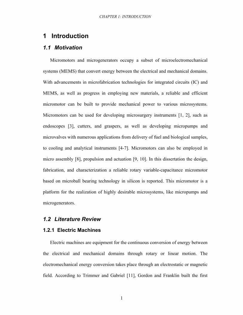
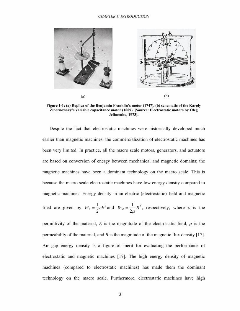
electrostatic motors in 1750s, 100 years before the advent of magnetic motors. The
replica of this motor made by the Electret Scientific Company is shown in Figure
1-1(a) [12]. The first capacitive electrostatic motor was developed during Edison’s
era in 1889 by Zipernowsky. The schematic of the motor is shown in Figure 1-1(b)
[12]. Peterson was also reported [13] to be one of the pioneers in development of
synchronous electrostatic motors in 1907. Nearly 50 years after Zipernowsky, Trump
discussed the concept, design, and fabrication of variable-capacitance machines [14,
15]. Trump explained the regime in which the machine acts as a motor or a generator,
demonstrated the average output electrical power of the generator, and discussed the
insulation problems of high-voltage electrostatic generators. Bollee published a
comprehensive study in 1969 on electrostatic motors in which he discussed the effects
of voltage excitation waveform, stator and rotor geometry, and ohmic and frictional
losses on the performance of the motor [13]. He elucidated the inherent tradeoffs in
the geometry design that would result in motors with high speed or high torque.
Mulcahy et al. demonstrate the fabrication of a macro scale 430-W vacuum-insulated
generator at 24 kV and 10000 rpm with 1 mm air gap between the stator and the rotor
[16].
CHAPTER 1: INTRODUCTION
3
(a)
(b)
Figure 1-1: (a) Replica of the Benjamin Franklin’s motor (1747), (b) schematic of the Karoly Zipernowsky’s variable capacitance motor (1889). [Source: Electrostatic motors by Oleg
Jefimenko, 1973].
Despite the fact that electrostatic machines were historically developed much
earlier than magnetic machines, the commercialization of electrostatic machines has
been very limited. In practice, all the macro scale motors, generators, and actuators
are based on conversion of energy between mechanical and magnetic domains; the
magnetic machines have been a dominant technology on the macro scale. This is
because the macro scale electrostatic machines have low energy density compared to
magnetic machines. Energy density in an electric (electrostatic) field and magnetic
filed are given by 2
21 EWE ε= and 2
21 BWM μ
= , respectively, where ε is the
permittivity of the material, E is the magnitude of the electrostatic field, μ is the
permeability of the material, and B is the magnitude of the magnetic flux density [17].
Air gap energy density is a figure of merit for evaluating the performance of
electrostatic and magnetic machines [17]. The high energy density of magnetic
machines (compared to electrostatic machines) has made them the dominant
technology on the macro scale. Furthermore, electrostatic machines have high
CHAPTER 1: INTRODUCTION
4
operating voltage and require precise geometry fabrication (especially at the air gap)
that is a disadvantage.
On the micro scale, however, the magnetic machines have several disadvantages.
Magnetic machines require use of ferromagnetic materials and thick metal layers that
are very challenging to fabricate and require processes that are not compatible with
traditional IC fabrication. These machines are current-driven and usually require large
driving currents. The current dissipates a lot of energy in the highly resistive micro
scale metal windings and magnetic core of the machine [18, 19]. One of the first
attempts on fabricating magnetic micromotors was reported by Dutta et al in 1970
[20].
In contrast, electrostatic machines are made of conductors and dielectrics which
are commonly used in conventional IC fabrication processes. In order to increase the
speed and functionality of integrated circuits the properties of conductors and
dielectrics have been optimized in the last few decades; the fabrication process of the
electrostatic micromachines is much easier than magnetic counterparts. Chapman and
Krein [17, 21] have shown that on the micro scale (few micrometers gap size), the
energy density (at the gap) of electrostatic and magnetic micromachines are
comparable. Therefore, from the performance point of view, the micro scale
electrostatic machines are comparable to the magnetic counterparts and in particular
cases the electrostatic machines may be superior.
Several types of micromotors and microgenerators have been widely studied;
permanent electret [22-25], piezo-electric [26-29], and ultrasonic [30, 31]
micromachines are a few examples. Variable-capacitance and electric induction are
CHAPTER 1: INTRODUCTION
5
two major types of electrostatic micromachines1. Variable-reluctance and magnetic
induction machines, being the magnetic equivalent of variable-capacitance and
electric induction machines, together with permanent magnet machines are the main
types of magnetic micromachines. Variable-capacitance micromotors that were
among the first fabricated microelectromechanical devices are discussed in detail in
the next section.
1.2.2 Variable-Capacitance Micromachines The operating principle of variable-capacitance micromachines is discussed in
Chapter 2. These are synchronous machines that produce torque due to spatial
misalignment of electrodes on the stator and salient poles on the rotor2. Trimmer and
Gabriel proposed the concept of linear and rotary variable-capacitance micromotors
(VCM) in 1987 [11]. The first generation of VCM was simultaneously developed by
two groups in the late 80’s: Tai et al. at the University of California, Berkeley [32,
33], and Mehregany et al. at the Massachusetts Institute of Technology (MIT) [34].
These were synchronous motors fabricated using semi-standard IC fabrication
processes known as “surface micromachining” [35]. Surface micromachining refers
to a fabrication process than in one of its steps involves selective removal of a film
(sacrificial layer) to release a structure. This type of micromachining, considered a
major MEMS fabrication process, is adopted from an earlier work in fabricating
resonant gate transistors [36]. The development of the variable-capacitance
micromotors was based on initial attempts of Lober and Howe on fabricating passive 1 Electric induction machines should not be confused with the conventional magnetic induction machines. 2 The definition of poles in the electrostatic machines may be different than their magnetic counterparts.
CHAPTER 1: INTRODUCTION
6
polysilicon structures together with a top-drive VCM [37]. Two similar fabrication
processes reported by Mehregany et al. were utilized for the fabrication of VCMs:
center-pin and flange [38, 39]. The rotor in these types of VCMs would sit on either
flanges or a center-pin. In these processes, thin films of silicon nitride and silicon
dioxide were used as an electrical insulator and sacrificial layer, while a polysilicon
film was used as a structural material. The design principles including the effect of
different geometries on the torque of the motor, as well as the fabrication and
dynamics of the machines were reported by Mehregany et al. [34, 39-41].
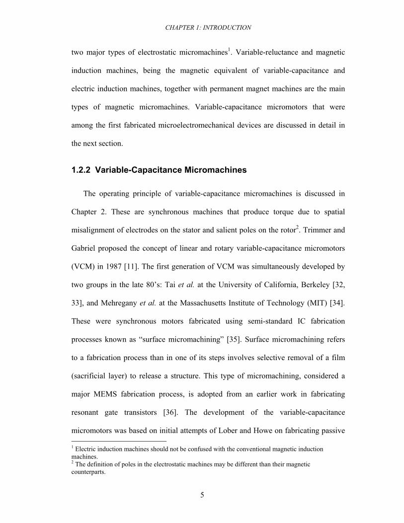
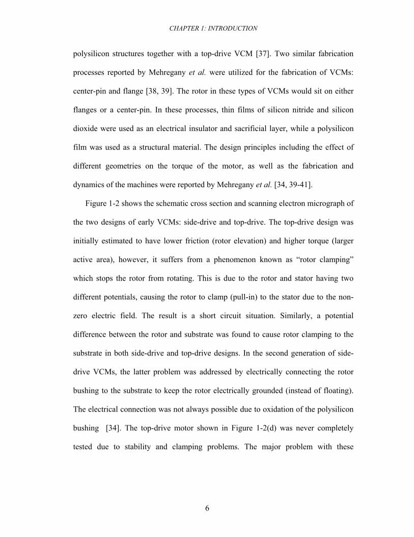
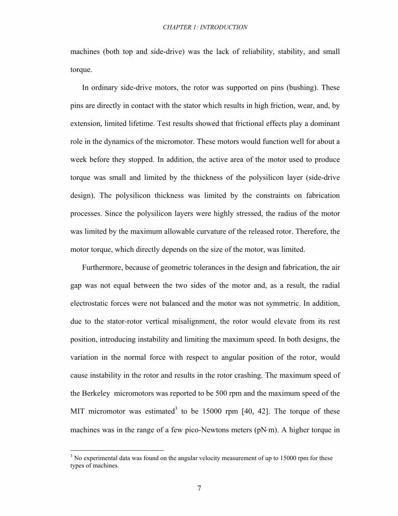
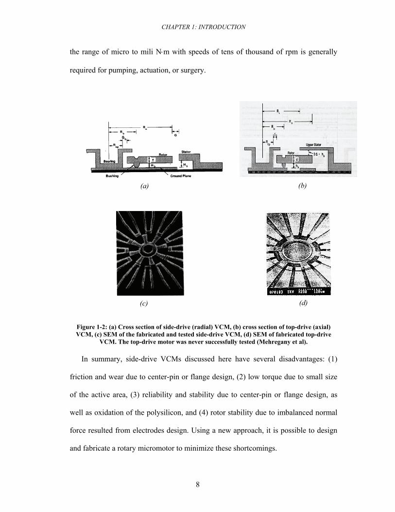
Figure 1-2 shows the schematic cross section and scanning electron micrograph of
the two designs of early VCMs: side-drive and top-drive. The top-drive design was
initially estimated to have lower friction (rotor elevation) and higher torque (larger
active area), however, it suffers from a phenomenon known as “rotor clamping”
which stops the rotor from rotating. This is due to the rotor and stator having two
different potentials, causing the rotor to clamp (pull-in) to the stator due to the non-
zero electric field. The result is a short circuit situation. Similarly, a potential
difference between the rotor and substrate was found to cause rotor clamping to the
substrate in both side-drive and top-drive designs. In the second generation of side-
drive VCMs, the latter problem was addressed by electrically connecting the rotor
bushing to the substrate to keep the rotor electrically grounded (instead of floating).
The electrical connection was not always possible due to oxidation of the polysilicon
bushing [34]. The top-drive motor shown in Figure 1-2(d) was never completely
tested due to stability and clamping problems. The major problem with these
CHAPTER 1: INTRODUCTION
7
machines (both top and side-drive) was the lack of reliability, stability, and small
torque.
In ordinary side-drive motors, the rotor was supported on pins (bushing). These
pins are directly in contact with the stator which results in high friction, wear, and, by
extension, limited lifetime. Test results showed that frictional effects play a dominant
role in the dynamics of the micromotor. These motors would function well for about a
week before they stopped. In addition, the active area of the motor used to produce
torque was small and limited by the thickness of the polysilicon layer (side-drive
design). The polysilicon thickness was limited by the constraints on fabrication
processes. Since the polysilicon layers were highly stressed, the radius of the motor
was limited by the maximum allowable curvature of the released rotor. Therefore, the
motor torque, which directly depends on the size of the motor, was limited.
Furthermore, because of geometric tolerances in the design and fabrication, the air
gap was not equal between the two sides of the motor and, as a result, the radial
electrostatic forces were not balanced and the motor was not symmetric. In addition,
due to the stator-rotor vertical misalignment, the rotor would elevate from its rest
position, introducing instability and limiting the maximum speed. In both designs, the
variation in the normal force with respect to angular position of the rotor, would
cause instability in the rotor and results in the rotor crashing. The maximum speed of
the Berkeley micromotors was reported to be 500 rpm and the maximum speed of the
MIT micromotor was estimated3 to be 15000 rpm [40, 42]. The torque of these
machines was in the range of a few pico-Newtons meters (pN⋅m). A higher torque in
3 No experimental data was found on the angular velocity measurement of up to 15000 rpm for these types of machines.
CHAPTER 1: INTRODUCTION
8
the range of micro to mili N⋅m with speeds of tens of thousand of rpm is generally
required for pumping, actuation, or surgery.
(c)
(a)
(d)
(b)
Figure 1-2: (a) Cross section of side-drive (radial) VCM, (b) cross section of top-drive (axial) VCM, (c) SEM of the fabricated and tested side-drive VCM, (d) SEM of fabricated top-drive
VCM. The top-drive motor was never successfully tested (Mehregany et al).
In summary, side-drive VCMs discussed here have several disadvantages: (1)
friction and wear due to center-pin or flange design, (2) low torque due to small size
of the active area, (3) reliability and stability due to center-pin or flange design, as
well as oxidation of the polysilicon, and (4) rotor stability due to imbalanced normal
force resulted from electrodes design. Using a new approach, it is possible to design
and fabricate a rotary micromotor to minimize these shortcomings.
CHAPTER 1: INTRODUCTION
9
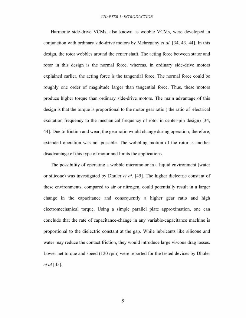
Harmonic side-drive VCMs, also known as wobble VCMs, were developed in
conjunction with ordinary side-drive motors by Mehregany et al. [34, 43, 44]. In this
design, the rotor wobbles around the center shaft. The acting force between stator and
rotor in this design is the normal force, whereas, in ordinary side-drive motors
explained earlier, the acting force is the tangential force. The normal force could be
roughly one order of magnitude larger than tangential force. Thus, these motors
produce higher torque than ordinary side-drive motors. The main advantage of this
design is that the torque is proportional to the motor gear ratio ( the ratio of electrical
excitation frequency to the mechanical frequency of rotor in center-pin design) [34,
44]. Due to friction and wear, the gear ratio would change during operation; therefore,
extended operation was not possible. The wobbling motion of the rotor is another
disadvantage of this type of motor and limits the applications.
The possibility of operating a wobble micromotor in a liquid environment (water
or silicone) was investigated by Dhuler et al. [45]. The higher dielectric constant of
these environments, compared to air or nitrogen, could potentially result in a larger
change in the capacitance and consequently a higher gear ratio and high
electromechanical torque. Using a simple parallel plate approximation, one can
conclude that the rate of capacitance-change in any variable-capacitance machine is
proportional to the dielectric constant at the gap. While lubricants like silicone and
water may reduce the contact friction, they would introduce large viscous drag losses.
Lower net torque and speed (120 rpm) were reported for the tested devices by Dhuler
et al [45].
CHAPTER 1: INTRODUCTION
10
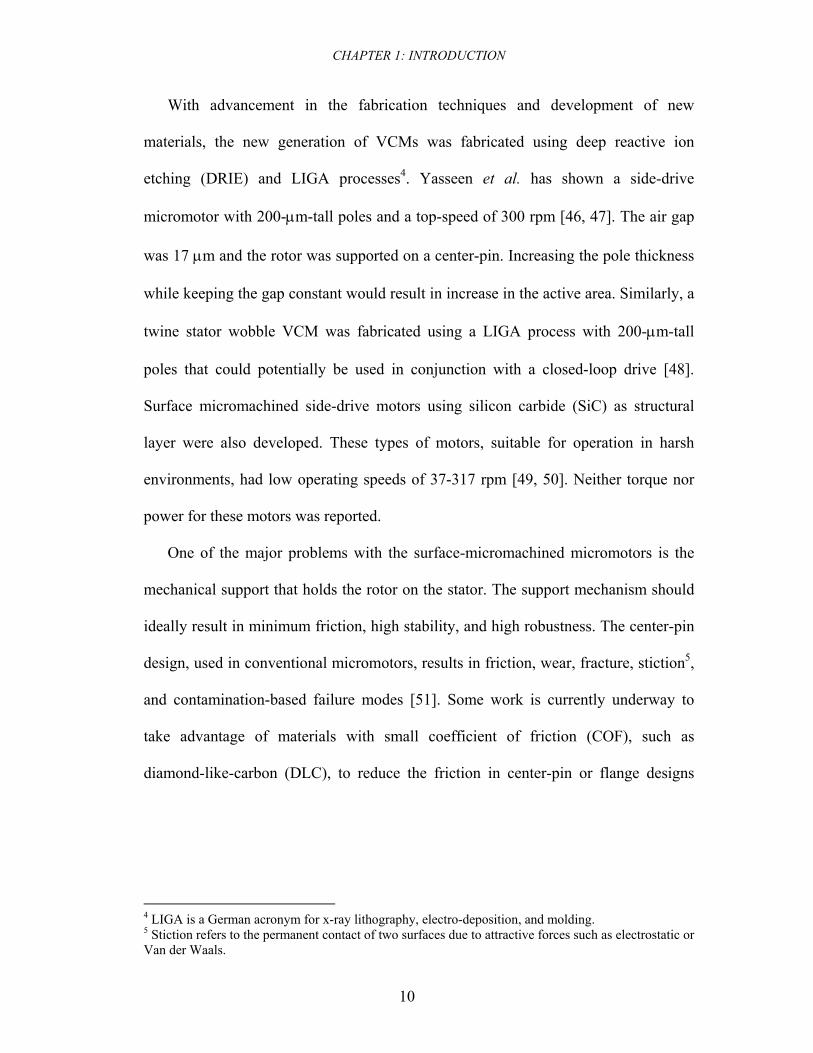
With advancement in the fabrication techniques and development of new
materials, the new generation of VCMs was fabricated using deep reactive ion
etching (DRIE) and LIGA processes4. Yasseen et al. has shown a side-drive
micromotor with 200-μm-tall poles and a top-speed of 300 rpm [46, 47]. The air gap
was 17 μm and the rotor was supported on a center-pin. Increasing the pole thickness
while keeping the gap constant would result in increase in the active area. Similarly, a
twine stator wobble VCM was fabricated using a LIGA process with 200-μm-tall
poles that could potentially be used in conjunction with a closed-loop drive [48].
Surface micromachined side-drive motors using silicon carbide (SiC) as structural
layer were also developed. These types of motors, suitable for operation in harsh
environments, had low operating speeds of 37-317 rpm [49, 50]. Neither torque nor
power for these motors was reported.
One of the major problems with the surface-micromachined micromotors is the
mechanical support that holds the rotor on the stator. The support mechanism should
ideally result in minimum friction, high stability, and high robustness. The center-pin
design, used in conventional micromotors, results in friction, wear, fracture, stiction5,
and contamination-based failure modes [51]. Some work is currently underway to
take advantage of materials with small coefficient of friction (COF), such as
diamond-like-carbon (DLC), to reduce the friction in center-pin or flange designs
4 LIGA is a German acronym for x-ray lithography, electro-deposition, and molding. 5 Stiction refers to the permanent contact of two surfaces due to attractive forces such as electrostatic or Van der Waals.
CHAPTER 1: INTRODUCTION
11
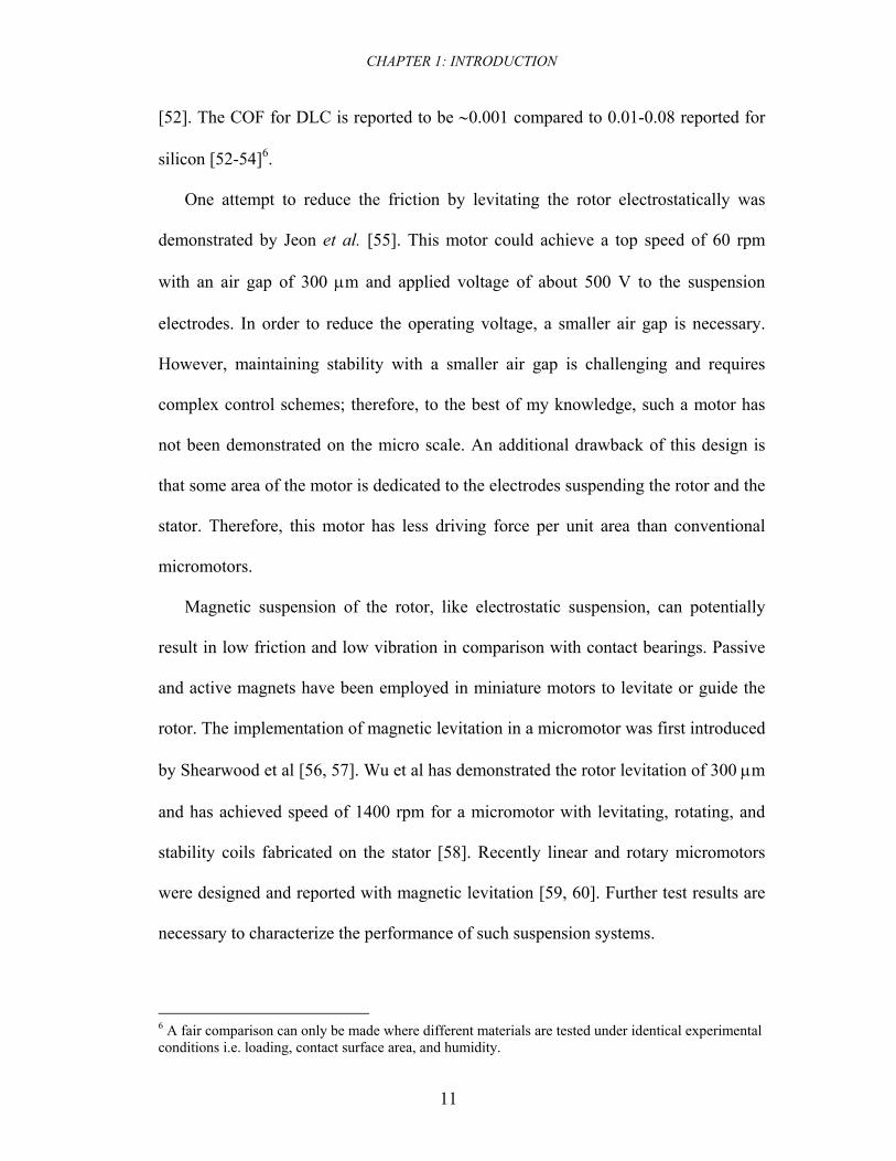
[52]. The COF for DLC is reported to be ∼0.001 compared to 0.01-0.08 reported for
silicon [52-54]6.
One attempt to reduce the friction by levitating the rotor electrostatically was
demonstrated by Jeon et al. [55]. This motor could achieve a top speed of 60 rpm
with an air gap of 300 μm and applied voltage of about 500 V to the suspension
electrodes. In order to reduce the operating voltage, a smaller air gap is necessary.
However, maintaining stability with a smaller air gap is challenging and requires
complex control schemes; therefore, to the best of my knowledge, such a motor has
not been demonstrated on the micro scale. An additional drawback of this design is
that some area of the motor is dedicated to the electrodes suspending the rotor and the
stator. Therefore, this motor has less driving force per unit area than conventional
micromotors.
Magnetic suspension of the rotor, like electrostatic suspension, can potentially
result in low friction and low vibration in comparison with contact bearings. Passive
and active magnets have been employed in miniature motors to levitate or guide the
rotor. The implementation of magnetic levitation in a micromotor was first introduced
by Shearwood et al [56, 57]. Wu et al has demonstrated the rotor levitation of 300 μm
and has achieved speed of 1400 rpm for a micromotor with levitating, rotating, and
stability coils fabricated on the stator [58]. Recently linear and rotary micromotors
were designed and reported with magnetic levitation [59, 60]. Further test results are
necessary to characterize the performance of such suspension systems.
6 A fair comparison can only be made where different materials are tested under identical experimental conditions i.e. loading, contact surface area, and humidity.
CHAPTER 1: INTRODUCTION
12
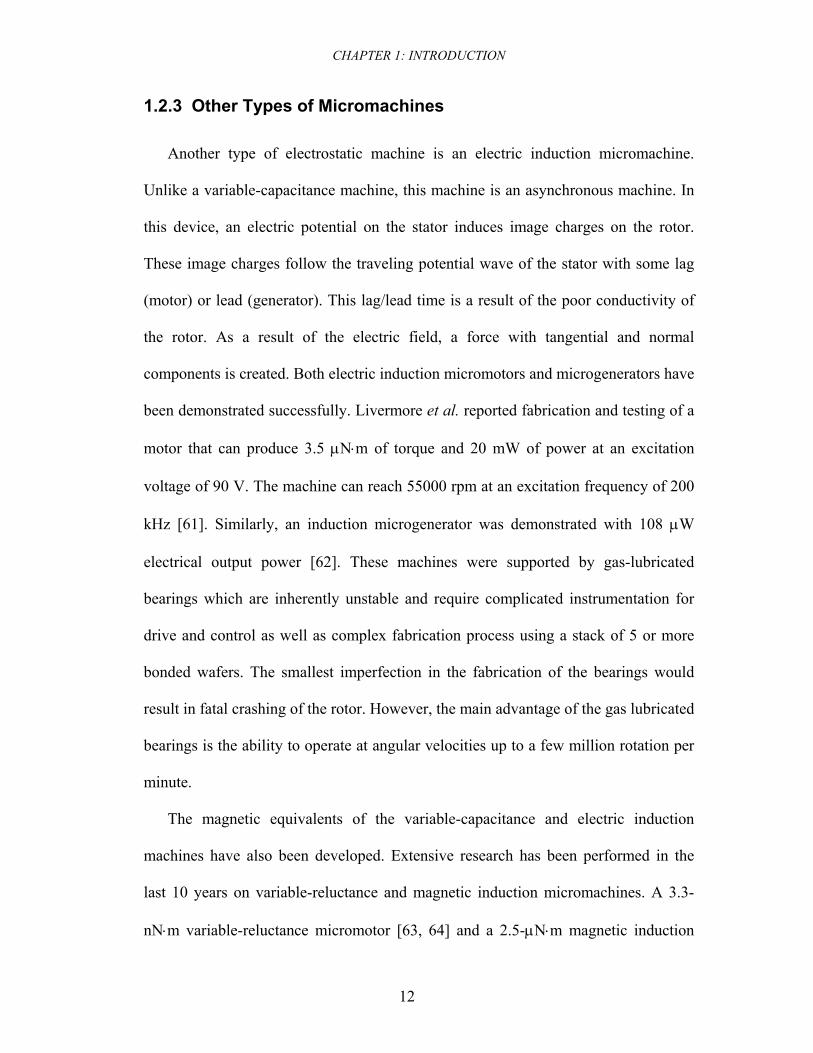
1.2.3 Other Types of Micromachines Another type of electrostatic machine is an electric induction micromachine.
Unlike a variable-capacitance machine, this machine is an asynchronous machine. In
this device, an electric potential on the stator induces image charges on the rotor.
These image charges follow the traveling potential wave of the stator with some lag
(motor) or lead (generator). This lag/lead time is a result of the poor conductivity of
the rotor. As a result of the electric field, a force with tangential and normal
components is created. Both electric induction micromotors and microgenerators have
been demonstrated successfully. Livermore et al. reported fabrication and testing of a
motor that can produce 3.5 μN⋅m of torque and 20 mW of power at an excitation
voltage of 90 V. The machine can reach 55000 rpm at an excitation frequency of 200
kHz [61]. Similarly, an induction microgenerator was demonstrated with 108 μW
electrical output power [62]. These machines were supported by gas-lubricated
bearings which are inherently unstable and require complicated instrumentation for
drive and control as well as complex fabrication process using a stack of 5 or more
bonded wafers. The smallest imperfection in the fabrication of the bearings would
result in fatal crashing of the rotor. However, the main advantage of the gas lubricated
bearings is the ability to operate at angular velocities up to a few million rotation per
minute.
The magnetic equivalents of the variable-capacitance and electric induction
machines have also been developed. Extensive research has been performed in the
last 10 years on variable-reluctance and magnetic induction micromachines. A 3.3-
nN⋅m variable-reluctance micromotor [63, 64] and a 2.5-μN⋅m magnetic induction
CHAPTER 1: INTRODUCTION
13
micromotor [18, 65] are two examples of these types of machines. A complete
review over design and analysis [66], fabrication and testing [67], eddy currents and
nonlinear effects [68] of the magnetic induction micromachines were recently
reported by Lang et al. The lack of reliable mechanical support is the major problem
in all these types of micromachines. The latter and the previously mentioned motors
[65], were all supported via an external shaft or a tether structure; whereas, the
electric induction micromotor [61] and the microgenerator [62] were supported on
gas-lubricated bearing, and the side-drive VCMs were supported on center-pin
structure [33, 39, 42].
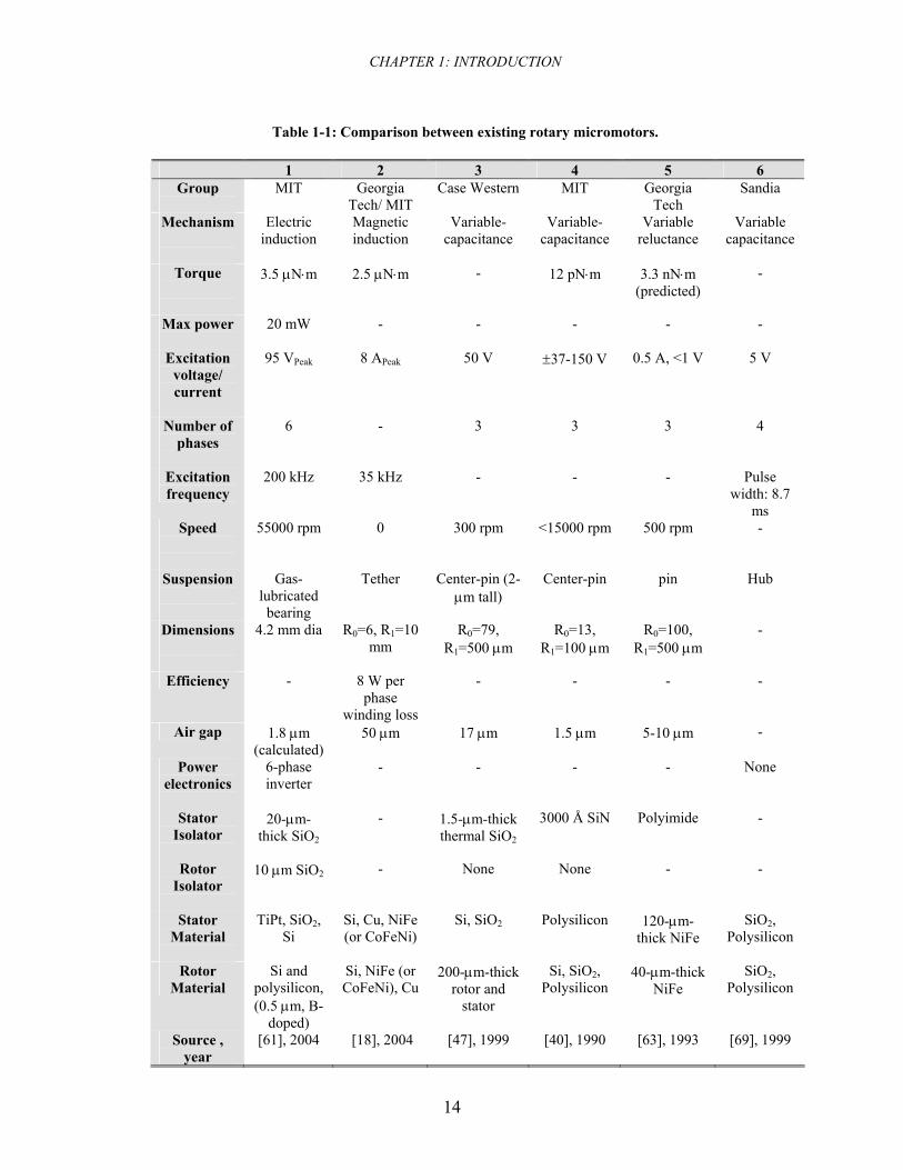
Table 1-1 summarizes the comparison between different types of rotary
micromotors reported in open literature [18, 40, 47, 61, 63, 69]. The key
specifications for these rotary machines including speed, torque, power, support
mechanism, and size are all given in this table. The parameters that were not
explicitly reported by the authors were left blank in the table (no presumption or
judgment was made even in obvious cases). All the micromotors listed suffer from
reliability problems associated with center-pin or gas-lubricated bearings.
CHAPTER 1: INTRODUCTION
14
Table 1-1: Comparison between existing rotary micromotors.
1 2 3 4 5 6 Group
MIT Georgia
Tech/ MIT Case Western MIT Georgia
Tech Sandia
Mechanism
Electric induction
Magnetic induction
Variable-capacitance
Variable-capacitance
Variable reluctance
Variable capacitance
Torque
3.5 μN⋅m 2.5 μN⋅m - 12 pN⋅m 3.3 nN⋅m (predicted)
-
Max power
20 mW - - - - -
Excitation voltage/ current
95 VPeak 8 APeak 50 V ±37-150 V 0.5 A, <1 V 5 V
Number of phases
6 - 3 3 3 4
Excitation frequency
200 kHz 35 kHz - - - Pulse width: 8.7
ms Speed
55000 rpm 0 300 rpm <15000 rpm 500 rpm -
Suspension
Gas-lubricated bearing
Tether Center-pin (2-μm tall)
Center-pin pin Hub
Dimensions
4.2 mm dia R0=6, R1=10 mm
R0=79, R1=500 μm
R0=13, R1=100 μm
R0=100, R1=500 μm
-
Efficiency - 8 W per phase
winding loss
- - - -
Air gap 1.8 μm (calculated)
50 μm 17 μm 1.5 μm 5-10 μm -
Power electronics
6-phase inverter
- - - - None
Stator Isolator
20-μm-thick SiO2
- 1.5-μm-thick thermal SiO2
3000 Å SiN Polyimide -
Rotor Isolator
10 μm SiO2 - None None - -
Stator Material
TiPt, SiO2, Si
Si, Cu, NiFe (or CoFeNi)
Si, SiO2 Polysilicon 120-μm-thick NiFe
SiO2, Polysilicon
Rotor Material
Si and polysilicon, (0.5 μm, B-
doped)
Si, NiFe (or CoFeNi), Cu
200-μm-thick rotor and
stator
Si, SiO2, Polysilicon
40-μm-thick NiFe
SiO2, Polysilicon
Source , year
[61], 2004 [18], 2004 [47], 1999 [40], 1990 [63], 1993 [69], 1999
CHAPTER 1: INTRODUCTION
15
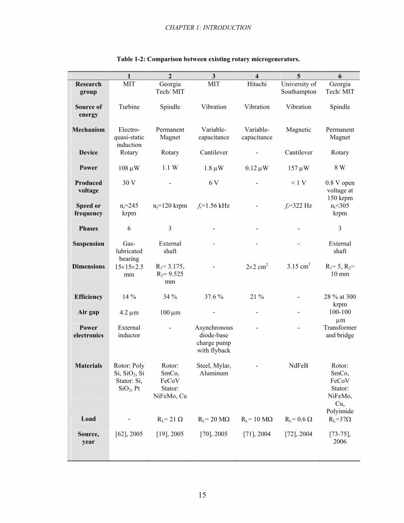
Table 1-2: Comparison between existing rotary microgenerators.
1 2 3 4 5 6 Research
group
MIT Georgia Tech/ MIT
MIT Hitachi University of Southampton
Georgia Tech/ MIT
Source of energy
Turbine Spindle Vibration Vibration Vibration Spindle
Mechanism
Electro-quasi-static induction
Permanent Magnet
Variable-capacitance
Variable-capacitance
Magnetic Permanent Magnet
Device
Rotary Rotary Cantilever - Cantilever Rotary
Power
108 μW 1.1 W 1.8 μW 0.12 μW 157 μW 8 W
Produced voltage
30 V - 6 V - < 1 V 0.8 V open voltage at 150 krpm
Speed or frequency
nr=245 krpm
nr=120 krpm fr=1.56 kHz - fr=322 Hz nr<305 krpm
Phases
6 3 - - - 3
Suspension
Gas-lubricated bearing
External shaft
- - - External shaft
Dimensions
15×15×2.5 mm
R1= 3.175, R2= 9.525
mm
- 2×2 cm2 3.15 cm3 R1= 5, R2= 10 mm
Efficiency
14 % 34 % 37.6 % 21 % - 28 % at 300 krpm
Air gap
4.2 μm 100 μm - - - 100-100 μm
Power electronics
External inductor
- Asynchronous diode-base
charge pump with flyback
- - Transformer and bridge
Materials
Rotor: Poly Si, SiO2, Si Stator: Si, SiO2, Pt
Rotor: SmCo, FeCoV Stator:
NiFeMo, Cu
Steel, Mylar, Aluminum
- NdFeB Rotor: SmCo, FeCoV Stator:
NiFeMo, Cu,
Polyimide Load
- RL= 21 Ω RL= 20 MΩ RL= 10 MΩ RL= 0.6 Ω RL=37Ω
Source, year
[62], 2005 [19], 2005 [70], 2005 [71], 2004 [72], 2004 [73-75], 2006
CHAPTER 1: INTRODUCTION
16
Table 1-2 provides a similar summary for microgenerators [19, 27, 62, 70-72].
Output power, speed, efficiency, size, and support mechanism are the key parameters
included in Table 2. The highest electric output power reported for a magnetic
induction microgenerator was 1.1 W at 120 krpm. This machine was tested using a
suspended spindle. Recently, an axial flux, permanent magnet generator was reported
to supply 8 W of DC power at 305 krpm [73]. Unlike an induction machine, the
permanent magnetic generator was a synchronous machine. Samarium-cobalt (SmCo)
rare-earth magnets were used for the rotor and Cu was used for the stator winding.
The machine was tested using a suspended spindle [74, 75].
1.2.4 Test and Characterization While a great deal of research has been conducted on the design and fabrication of
micromachines, little work has been published on drive, control, and characterization
of these machines. Electrostatic micromotors, in general, require multi-phase high-
voltage drives. Depending on the voltage amplitude, frequency, duty cycle, phase
difference, number of phases, and the type of wave-form, an in-house power
electronics system is generally required. Maintaining the integrity of the wave-form
delivered to the capacitive load (with stringent timing constraints) makes the circuit
design challenging. One example of such a system developed by Neugebauer et al. is
capable of operating up to 300 V and 2 MHz [76].
In some machines, the optimal driving requires instantaneous rotor position
information. Therefore, a more robust and reliable control scheme for the most
micromotors is a closed-loop control. This is more important in variable-capacitance
motors since they are synchronous machines. With a feedback circuit, a micromotor
CHAPTER 1: INTRODUCTION
17
can be controlled to operate at a desired (steady) speed and torque. Some preliminary
work has been performed for driving side-drive VCMs in a closed-loop fashion by
sensing the capacitance-change of each phase using a high-frequency signal
(modulated on the main drive signals) and a capacitance sensing circuit [77]. Optical
position sensing can also be used; however, the integration of optical sources and
detectors with a micromotor is challenging. This research is currently underway at the
University of Maryland (UMD). Other approaches have been proposed to eliminate
the need for capacitance sensing circuit by implementing a segmented bearing design
in a wobble VCM [48]. As the rotor rolls around the segmented bearing, the gap
between 2 adjacent bearing segments is bridged by the rotor and the momentary
electrical short circuit can be sensed by the electronics and used to determine the
position of the rotor. It was also shown that drive electronics can be monolithically
integrated with the micromotor on a single chip using complementary metal-oxide-
semiconductor (CMOS) processes. In this approach a surface micromachined VCM
was integrated with a CMOS drive circuit containing an oscillator, a frequency
divider, and double-diffused MOS transistors [78].
Characterization of the micromotors is usually performed by measuring speed,
torque, and output power. Efficiency is also a key parameter determining the
performance of the micromotor. Bart et al. has characterized the dynamic behavior of
side-drive VCMs through the use of stroboscopic dynamometry [79, 80] and
estimated the drive torque and friction parameters. Direct torque measurement has
also been shown for wobble motors by measuring the deflection of a long cantilever
beam fixed at one end and connected to the motor rotor via a surface-micromachined
CHAPTER 1: INTRODUCTION
18
gear structure at the other end [81, 82]. Non-contact torque measurement has been
demonstrated in electric induction motors by removing the stator excitation and
monitoring the rotor deceleration (with respect to time) with optical displacement
sensors [61]. With this method, torques less than 3.5 μN⋅m were indirectly measured.
While the output power of electrostatic motors can be estimated using similar
methods, the measurement of the input power is not trivial and involves measuring
currents in the range of a few pico-amps or less. An alternating current (AC) ammeter
is necessary since the motor is a capacitive load. In summary, stringent driving
requirements and the small size of the device makes the test and characterization of
micromotors challenging.
1.3 Development of Micromachines at MSAL
Since August 2002, we have been involved in a development of a linear variable-
capacitance micromotor supported on microball bearings at the MEMS Sensors and
Actuators Lab (MSAL), University of Maryland. We initially demonstrated the
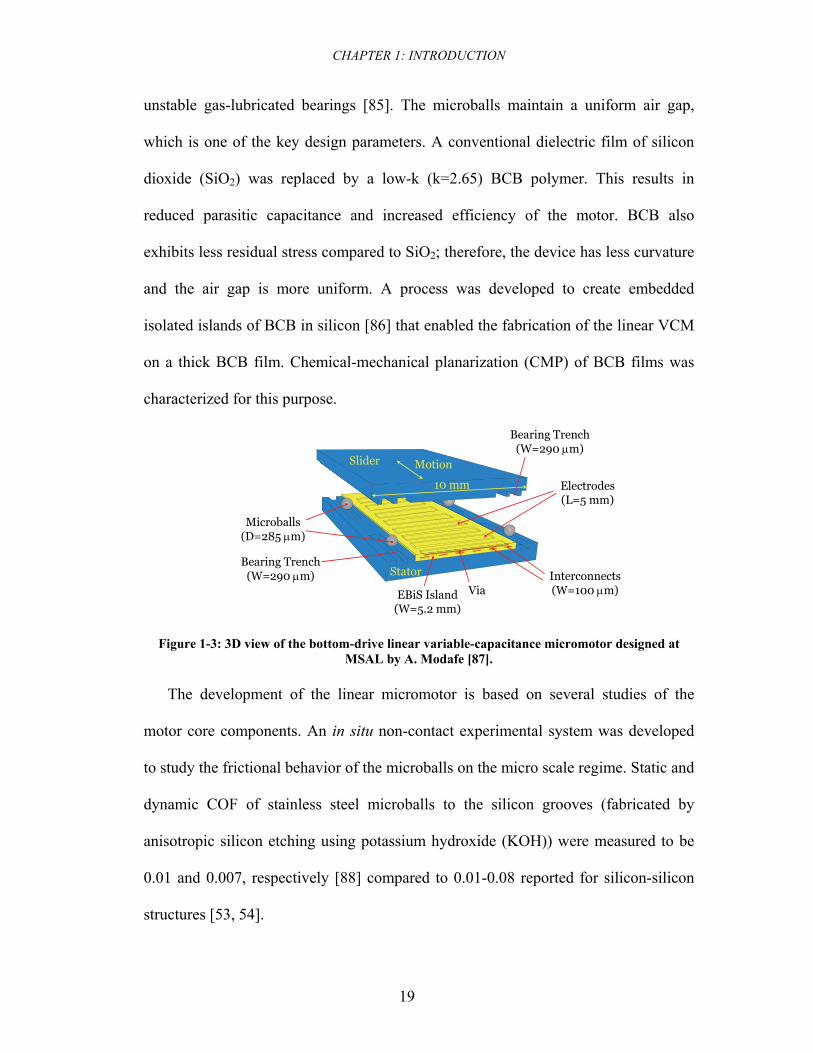
successful operation of this device in a 3-phase configuration [83]. Figure 1-3 shows
the 3D exploded view of the designed structure. Unlike the conventional VCMs that
were side-drive, this micromotor has a bottom-drive design which increases the active
area of the motor. Two new technologies were implemented in the development of
the linear micromotor: (1) microball bearing technology in silicon as a support
mechanism and (2) benzocyclobutene (BCB) low-k polymer as an insulating layer
[84]. The microball bearing technology results in stable and robust mechanical
support. The rolling microballs, sandwiched between rotor and stator, results in less
friction and wear when compared to center-pin design and are more reliable than
CHAPTER 1: INTRODUCTION
19
unstable gas-lubricated bearings [85]. The microballs maintain a uniform air gap,
which is one of the key design parameters. A conventional dielectric film of silicon
dioxide (SiO2) was replaced by a low-k (k=2.65) BCB polymer. This results in
reduced parasitic capacitance and increased efficiency of the motor. BCB also
exhibits less residual stress compared to SiO2; therefore, the device has less curvature
and the air gap is more uniform. A process was developed to create embedded
isolated islands of BCB in silicon [86] that enabled the fabrication of the linear VCM
on a thick BCB film. Chemical-mechanical planarization (CMP) of BCB films was
characterized for this purpose.
Slider
Stator
Motion
Microballs(D=285 μm)
Electrodes(L=5 mm)
Interconnects(W=100 μm)ViaEBiS Island
(W=5.2 mm)
Bearing Trench(W=290 μm)
Bearing Trench(W=290 μm)
10 mm
Figure 1-3: 3D view of the bottom-drive linear variable-capacitance micromotor designed at MSAL by A. Modafe [87].
The development of the linear micromotor is based on several studies of the
motor core components. An in situ non-contact experimental system was developed
to study the frictional behavior of the microballs on the micro scale regime. Static and
dynamic COF of stainless steel microballs to the silicon grooves (fabricated by
anisotropic silicon etching using potassium hydroxide (KOH)) were measured to be
0.01 and 0.007, respectively [88] compared to 0.01-0.08 reported for silicon-silicon
structures [53, 54].
CHAPTER 1: INTRODUCTION
20
The electrical properties of the BCB and the effect of environment (e.g. humidity)
on them are critical issues that affect the reliability of the micromotor. The dielectric
constant and breakdown voltage of BCB were measured and the effect of humidity on
these properties was studied [89]. The dielectric constant of BCB was measured to be
2.49 in dry environment. The dielectric constant was only increased by 1.2 % after a
humidity stress of 85 % RH at 85 °C. The study of the I-V characteristics of BCB
showed that humidity stress reduces the breakdown strength by a factor of 2-3 and
increases the maximum leakage current 10 fold.
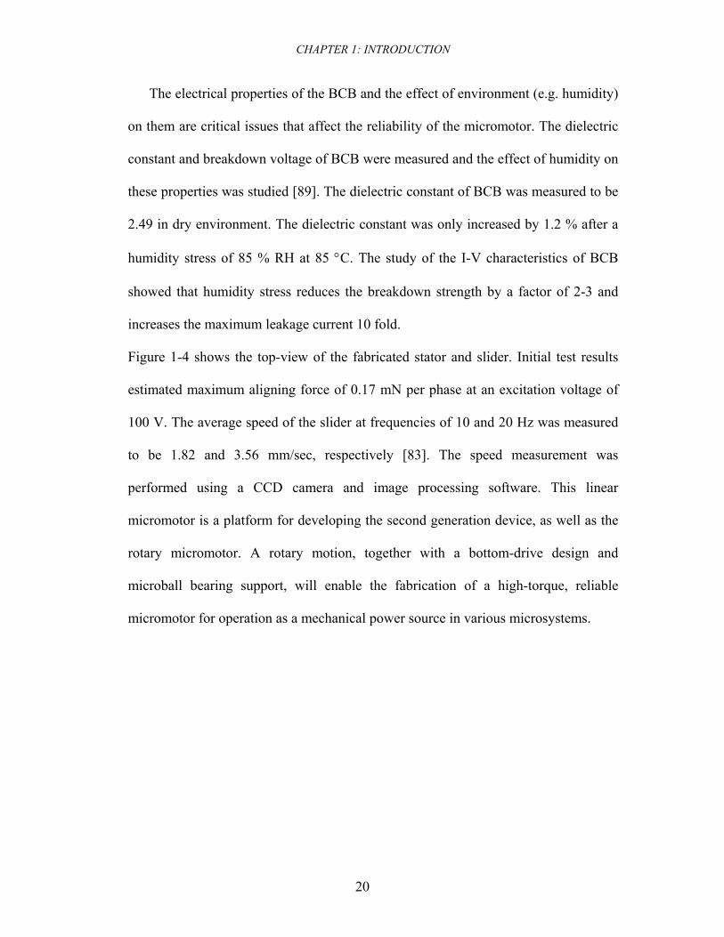
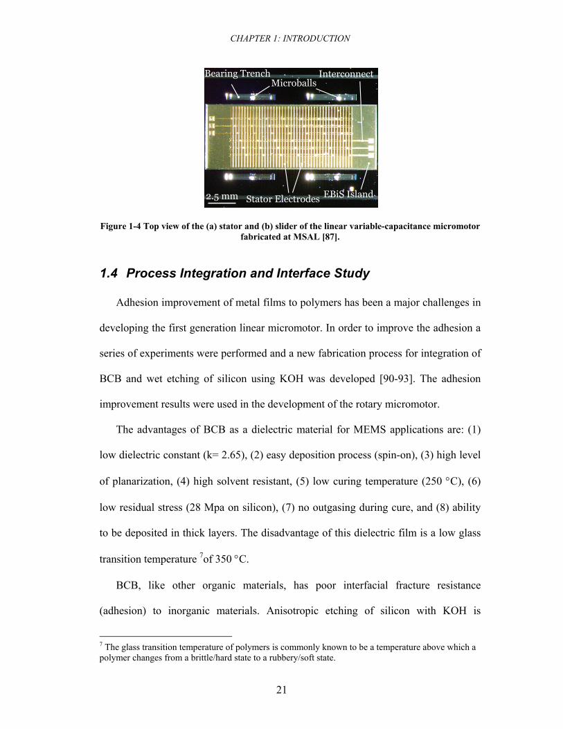
Figure 1-4 shows the top-view of the fabricated stator and slider. Initial test results
estimated maximum aligning force of 0.17 mN per phase at an excitation voltage of
100 V. The average speed of the slider at frequencies of 10 and 20 Hz was measured
to be 1.82 and 3.56 mm/sec, respectively [83]. The speed measurement was
performed using a CCD camera and image processing software. This linear
micromotor is a platform for developing the second generation device, as well as the
rotary micromotor. A rotary motion, together with a bottom-drive design and
microball bearing support, will enable the fabrication of a high-torque, reliable
micromotor for operation as a mechanical power source in various microsystems.
CHAPTER 1: INTRODUCTION
21
MicroballsInterconnectBearing Trench
2.5 mm EBiS IslandStator Electrodes
Figure 1-4 Top view of the (a) stator and (b) slider of the linear variable-capacitance micromotor fabricated at MSAL [87].
1.4 Process Integration and Interface Study
Adhesion improvement of metal films to polymers has been a major challenges in
developing the first generation linear micromotor. In order to improve the adhesion a
series of experiments were performed and a new fabrication process for integration of
BCB and wet etching of silicon using KOH was developed [90-93]. The adhesion
improvement results were used in the development of the rotary micromotor.
The advantages of BCB as a dielectric material for MEMS applications are: (1)
low dielectric constant (k= 2.65), (2) easy deposition process (spin-on), (3) high level
of planarization, (4) high solvent resistant, (5) low curing temperature (250 °C), (6)
low residual stress (28 Mpa on silicon), (7) no outgasing during cure, and (8) ability
to be deposited in thick layers. The disadvantage of this dielectric film is a low glass
transition temperature 7of 350 °C.
BCB, like other organic materials, has poor interfacial fracture resistance
(adhesion) to inorganic materials. Anisotropic etching of silicon with KOH is
7 The glass transition temperature of polymers is commonly known to be a temperature above which a polymer changes from a brittle/hard state to a rubbery/soft state.
CHAPTER 1: INTRODUCTION
22
performed in a very corrosive environment at high temperatures for a few hours.
Therefore, it is essential to protect the BCB film during this process with an etch
mask. It was shown that fabrication of deep silicon etched structures together with
BCB dielectric films can be preformed using appropriate metal etch masks (Au/Cr)
with a modified process flow to enhance the metal/BCB adhesion.
A series of experiments were performed to modify the fabrication process such
that the adhesion between metal and BCB becomes strong. Adhesion improvement of
BCB and Cr/Au etch mask was accomplished by partial cure of BCB prior to
metallization, sputtering of the Cr/Au metal masks at 200 °C, and full curing at 250
°C. An adhesion promoter, AP3000, was proven to enhance the adhesion of these
films if applied prior to metallization. Metal/BCB adhesion was tested to be very
strong. Adhesion strength was experimentally verified in a qualitative manner. Deep
structures (200 μm) in silicon were fabricated while the BCB film was protected by
metal mask. Long exposure to KOH solution (8 h) had little or no effect on the
adhesion of polymer- metal. The process was repeatable, giving the same set of
results.
In order to understand the effect of soft cure and adhesion promoter prior to
metallization and hard cure after metallization, the metal/BCB interface was studied.
Different surface/interface techniques were used. Time-of-flight secondary ion mass
spectroscopy (ToF-SIMS), Auger electron spectroscopy (AES), secondary electron
spectroscopy (SEM), and atomic force microscopy (AFM) were the methods
exercised along with 12 samples fabricated with different stacks of films for this
study.
CHAPTER 1: INTRODUCTION
23
High lateral resolution ToF-SIMS imaging provided useful information about the
surface of the Au and Cr (grain sizes) inside the Au layer. These images showed that
the Cr diffusion (after curing) into Au layer was not homogeneous. Chromium-
enriched grains of 2 μm or smaller were detected close to pure Au grains. The
masking strength of the Au layer (against KOH) was not deteriorated by Cr diffusion.
AES was used to quantify the atomic concentration of Cr diffused into Au. The Cr
concentration at the Au layer was estimated to be 1 atomic percent on average.
Morphology of the BCB, Cr, and Au surfaces and the effect of hard cure on their
roughness were studied using AFM and SEM.
ToF-SIMS depth profiling was used for studying the interface of
Au/Cr/AP3000/BCB. Concentration of different species at different depths from the
surface of the wafer was measured. It was found that curing at 250 °C, together with
use of adhesion promoter on partially cured BCB results in diffusion of Si and C from
the BCB or AP3000 into the Cr layer. Use of cure management or adhesion promoter
alone did not result in adhesion improvement. Chemical interaction of BCB and Cr at
the interface, mainly in the form of oxidation of Cr, was also observed. Diffusion of
Si and C from BCB or AP3000 into the Cr layer together with the formation of
chromium-oxide at the Cr/BCB interface were correlated to the adhesion
improvement between BCB and Cr/Au films.
This integration enabled the fabrication process development for the linear
micromotor with 1 μm thick BCB film; however, if thicker BCB films are necessary
in future linear micromotors, modified methods can be implemented. The results from
this study were extensively used in the fabrication process of the rotary micromotor,
CHAPTER 1: INTRODUCTION
24
especially for two level metallization and three level BCB deposition steps. However,
DRIE was utilized instead of KOH to fabricate rotary microball housings.
1.5 Structure of the Manuscript
In the first chapter, the history and background of micromachines were discussed.
The proposed micromotor, theory of operation, microball bearing technology in
silicon, and derivation of machine velocity, torque, and efficiency are presented in
Chapter 2. The detailed design and finite element simulation, together with design
variation and mask layouts of the micromotor are presented in Chapter 3. Chapter 4
will address the fabrication challenges and final results for the stator and rotor. The
design, fabrication, and characterization of the rotary micromotor are based on prior
work on optimization of the linear micromotor. The characterization results for the
second-generation linear micromotor as well as the rotary machine are both reported
in Chapter 5. First, the characterization methodology and system modeling for the
linear micromotor are reported in Section 5.1. Second, test and characterization of the
rotary device, including steady-state and transient analysis, of the motion dynamics
i.e. position, velocity, acceleration, torque, and friction are discussed in Section 5.2. A
summary of the dissertation, future work, and concluding remarks are discussed in
Chapter 6.
CHAPTER 2: ROTARY MICROMOTOR-THEORY AND OPERATION
25
2 Rotary Micromotor: Theory and Operation
2.1 Overview
The micromotor developed in this work is a six-phase, bottom-drive, rotary,
variable-capacitance machine with a robust mechanical support provided by
microball bearings. The device is the first demonstration of a rotary micromotor using
microball bearing technology. In this chapter, a short overview of the design,
fabrication, and testing of the micromotor is presented, followed by reviewing two
core technologies: microball bearings and BCB. The theory of operation and the
derivation of velocity, torque, and efficiency of the machine are discussed.
2.1.1 Design
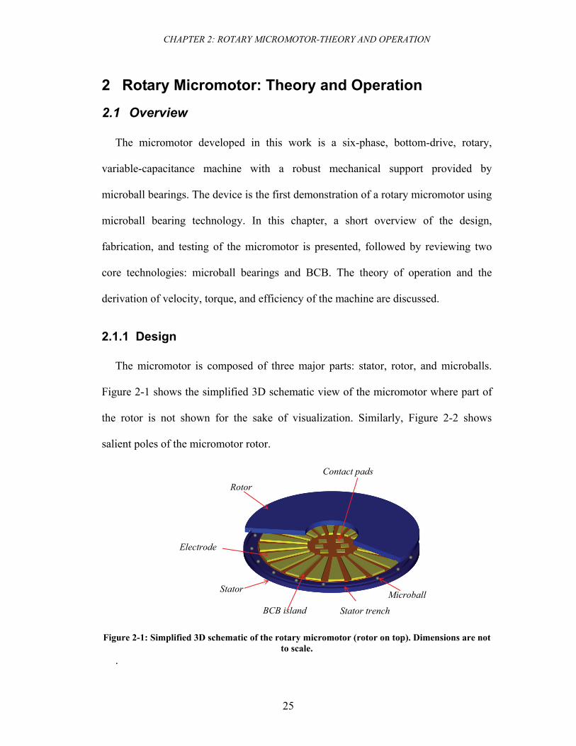
The micromotor is composed of three major parts: stator, rotor, and microballs.
Figure 2-1 shows the simplified 3D schematic view of the micromotor where part of
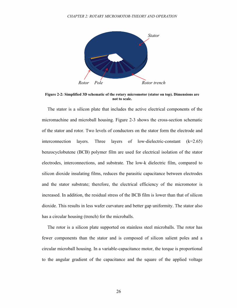
the rotor is not shown for the sake of visualization. Similarly, Figure 2-2 shows
salient poles of the micromotor rotor.
Rotor
Stator
Stator trench
Microball
Electrode
Contact pads
BCB island
Figure 2-1: Simplified 3D schematic of the rotary micromotor (rotor on top). Dimensions are not to scale.
.
CHAPTER 2: ROTARY MICROMOTOR-THEORY AND OPERATION
26
Pole
Stator
Rotor Rotor trench
Figure 2-2: Simplified 3D schematic of the rotary micromotor (stator on top). Dimensions are not to scale.
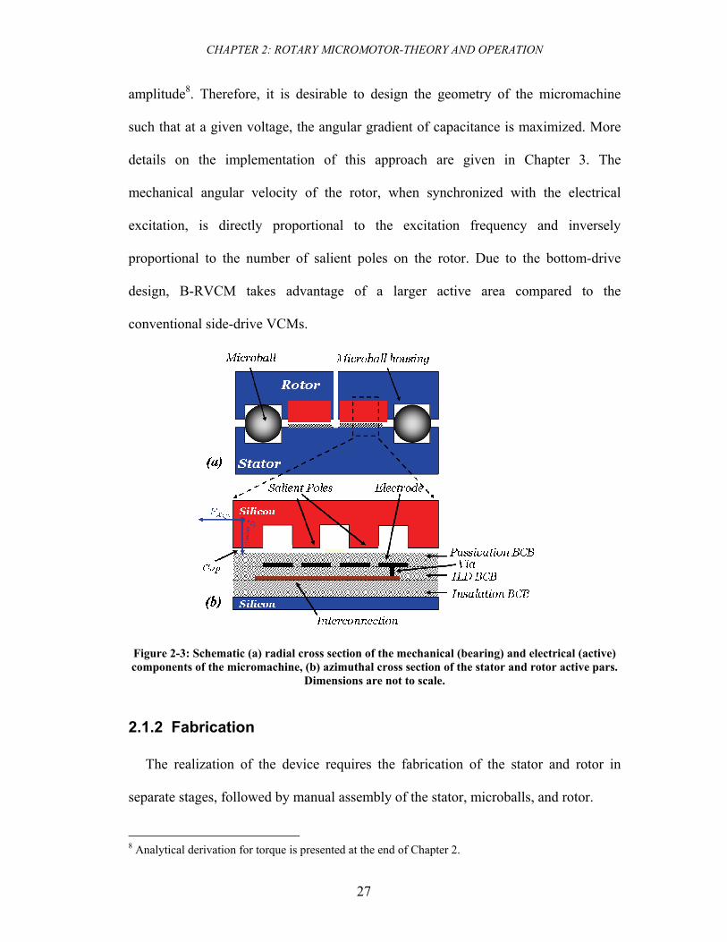
The stator is a silicon plate that includes the active electrical components of the
micromachine and microball housing. Figure 2-3 shows the cross-section schematic
of the stator and rotor. Two levels of conductors on the stator form the electrode and
interconnection layers. Three layers of low-dielectric-constant (k=2.65)
benzocyclobutene (BCB) polymer film are used for electrical isolation of the stator
electrodes, interconnections, and substrate. The low-k dielectric film, compared to
silicon dioxide insulating films, reduces the parasitic capacitance between electrodes
and the stator substrate; therefore, the electrical efficiency of the micromotor is
increased. In addition, the residual stress of the BCB film is lower than that of silicon
dioxide. This results in less wafer curvature and better gap uniformity. The stator also
has a circular housing (trench) for the microballs.
The rotor is a silicon plate supported on stainless steel microballs. The rotor has
fewer components than the stator and is composed of silicon salient poles and a
circular microball housing. In a variable-capacitance motor, the torque is proportional
to the angular gradient of the capacitance and the square of the applied voltage
CHAPTER 2: ROTARY MICROMOTOR-THEORY AND OPERATION
27
amplitude8. Therefore, it is desirable to design the geometry of the micromachine
such that at a given voltage, the angular gradient of capacitance is maximized. More
details on the implementation of this approach are given in Chapter 3. The
mechanical angular velocity of the rotor, when synchronized with the electrical
excitation, is directly proportional to the excitation frequency and inversely
proportional to the number of salient poles on the rotor. Due to the bottom-drive
design, B-RVCM takes advantage of a larger active area compared to the
conventional side-drive VCMs.
Figure 2-3: Schematic (a) radial cross section of the mechanical (bearing) and electrical (active) components of the micromachine, (b) azimuthal cross section of the stator and rotor active pars.
Dimensions are not to scale.
2.1.2 Fabrication
The realization of the device requires the fabrication of the stator and rotor in
separate stages, followed by manual assembly of the stator, microballs, and rotor.
8 Analytical derivation for torque is presented at the end of Chapter 2.
CHAPTER 2: ROTARY MICROMOTOR-THEORY AND OPERATION
28
As shown in Figure 2-3 the stator is composed of three layers of BCB film
(dielectric) and two layers of metal film (conductor). It is important that the first
metal layer be electrically insulated from the substrate. The parasitic capacitance
between this layer and the substrate needs to be minimized. Two metals are
electrically isolated and selectively connected to one another to form a six phase
machine. Uniform dielectric deposition is necessary to avoid electric breakdown at
sharp metal edges. The top electrode is passivated to reduce the chances of electric
breakdown during testing. The resistance between the two metal lines should be
minimal to reduce the time-constant and loss of the system. The BCB deposition is
performed using spinning and curing steps. The metal deposition is performed by DC
magnetron sputtering.
The mechanical support of the rotor is provided by fabrication of microball
housings in both stator and rotor. The uniformity of the microball housing plays an
important role in the gap uniformity. The rotor also has salient structures etched deep
into the silicon using DRIE. In order to minimize the fabrication steps, the rotor
housing and poles can be etched simultaneously. The rotor is released using DRIE
before testing.
2.1.3 Characterization
Test and characterization of the rotary variable-capacitance micromotor require
voltage excitation of 6 phases with large amplitude (∼150 V), specific phase
difference, frequency, and duty cycle. The motor is excited using a custom-designed
power electronic system composed of a PC, LabView program, data acquisition card,
and external high-voltage amplifier. The synchronization of the rotor motion with
CHAPTER 2: ROTARY MICROMOTOR-THEORY AND OPERATION
29
electrical excitation of the stator is automatically accomplished due to the inherent
characteristics of the machine later discussed in this Chapter. An opening in the rotor
is designed such that it allows the physical contact of the 6 probe needles with stator
pads. Without the presence of this opening, the fabrication process of the motor
would have been significantly more complicated.
The test setup is also composed of a motion characterization component for
measuring the angular position of the rotor. Two sets of measurements are performed
to characterize the motion: steady state and transient. The steady state response is
measured using a fiber-optic displacement sensor. These sensors are composed of a
source and intensity detector that detects the position of etched marks on the rotor.
The speed of the rotor is measured with this method. The transient response of the
motor is measured using a high-speed, high-resolution camera system. The torque of
the device, frictional forces, and the coefficient of friction are extracted from the
transient response tests. In these tests, the deceleration of the rotor motion is
calculated through numerical differentiation of angular position.
2.2 Microball Bearings Technology in Silicon
Mechanical support is one of the major challenges in development of
microelectromechanical devices especially micromotors and microgenerators. Ideally
the mechanical support would be reliable and stable with low friction and high
resistance to fracture and wear. Major technologies used as a mechanical support in
MEMS were reviewed in Chapter 1.
CHAPTER 2: ROTARY MICROMOTOR-THEORY AND OPERATION
30
2.2.1 Mechanical Support in MEMS
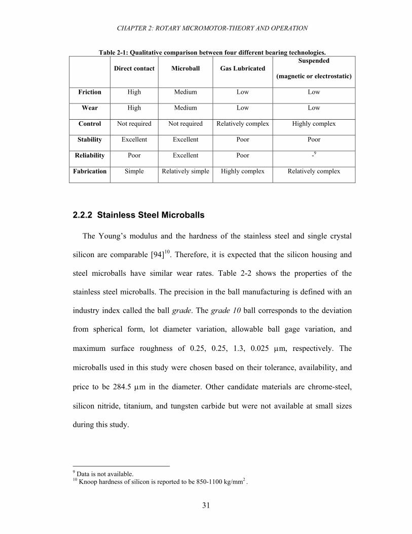
The microball bearing is the core technology used in the development of the rotary
micromotor. Table 2-1 summarizes a qualitative comparison between four different
support mechanisms: direct contact bearings (bushing), microball bearings, gas-
lubricated bearings, and magnetically or electrostatically suspended bearings. The
rolling microballs have less friction and higher wear resistance than contact or sliding
bearings. The fabrication of the micromachines based on this technology is
significantly less complicated than gas-lubricated bearings which generally require
tight fabrication tolerances for the journal and thrust bearings, as well as complex
fabrication scheme using 5-6 wafer level bonding processes. Furthermore, the
microball bearings are more stable than hydrostatic or hydrodynamic gas-lubricated
bearings and require no control scheme; whereas, in gas lubricated bearings startup
and active control are one of the many challenges.
The other important advantage of the microball bearing technology is the ability to
define and sustain a uniform gap across the active area of the micromotor due to its
contact nature. This property is significantly important for variable-capacitance
micromachines for two obvious reasons: the air gap needs to be as small as possible
and the active area of the micromotor at the gap needs to be large. Practically, the
design of the machine dictates the small gap in the range of 10 μm with active areas
in range of 10-100 mm2. Microball bearings enable the design of the micromotors that
have a small air gap with large active area and therefore high torque. The uncertainty
in gap will be dictated by the accuracy in trench depth and ball diameter.
CHAPTER 2: ROTARY MICROMOTOR-THEORY AND OPERATION
31
Table 2-1: Qualitative comparison between four different bearing technologies.
Direct contact Microball Gas Lubricated Suspended
(magnetic or electrostatic)
Friction High Medium Low Low
Wear High Medium Low Low
Control Not required Not required Relatively complex Highly complex
Stability Excellent Excellent Poor Poor
Reliability Poor Excellent Poor -9
Fabrication Simple Relatively simple Highly complex Relatively complex
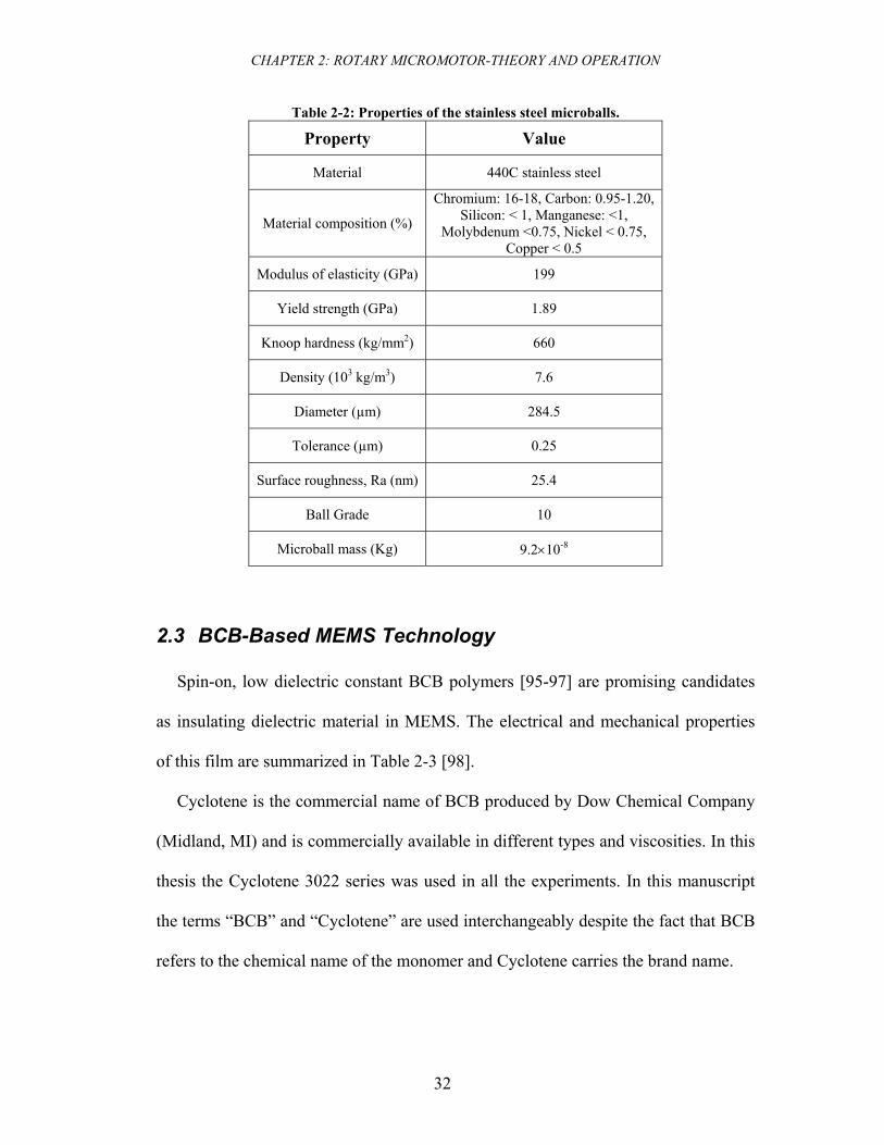
2.2.2 Stainless Steel Microballs
The Young’s modulus and the hardness of the stainless steel and single crystal
silicon are comparable [94]10. Therefore, it is expected that the silicon housing and
steel microballs have similar wear rates. Table 2-2 shows the properties of the
stainless steel microballs. The precision in the ball manufacturing is defined with an
industry index called the ball grade. The grade 10 ball corresponds to the deviation
from spherical form, lot diameter variation, allowable ball gage variation, and
maximum surface roughness of 0.25, 0.25, 1.3, 0.025 μm, respectively. The
microballs used in this study were chosen based on their tolerance, availability, and
price to be 284.5 μm in the diameter. Other candidate materials are chrome-steel,
silicon nitride, titanium, and tungsten carbide but were not available at small sizes
during this study.
9 Data is not available. 10 Knoop hardness of silicon is reported to be 850-1100 kg/mm2 .
CHAPTER 2: ROTARY MICROMOTOR-THEORY AND OPERATION
32
Table 2-2: Properties of the stainless steel microballs.
Property Value
Material 440C stainless steel
Material composition (%)
Chromium: 16-18, Carbon: 0.95-1.20, Silicon: < 1, Manganese: <1,
Molybdenum <0.75, Nickel < 0.75, Copper < 0.5
Modulus of elasticity (GPa) 199
Yield strength (GPa) 1.89
Knoop hardness (kg/mm2) 660
Density (103 kg/m3) 7.6
Diameter (µm) 284.5
Tolerance (µm) 0.25
Surface roughness, Ra (nm) 25.4
Ball Grade 10
Microball mass (Kg) 9.2×10⁻⁸
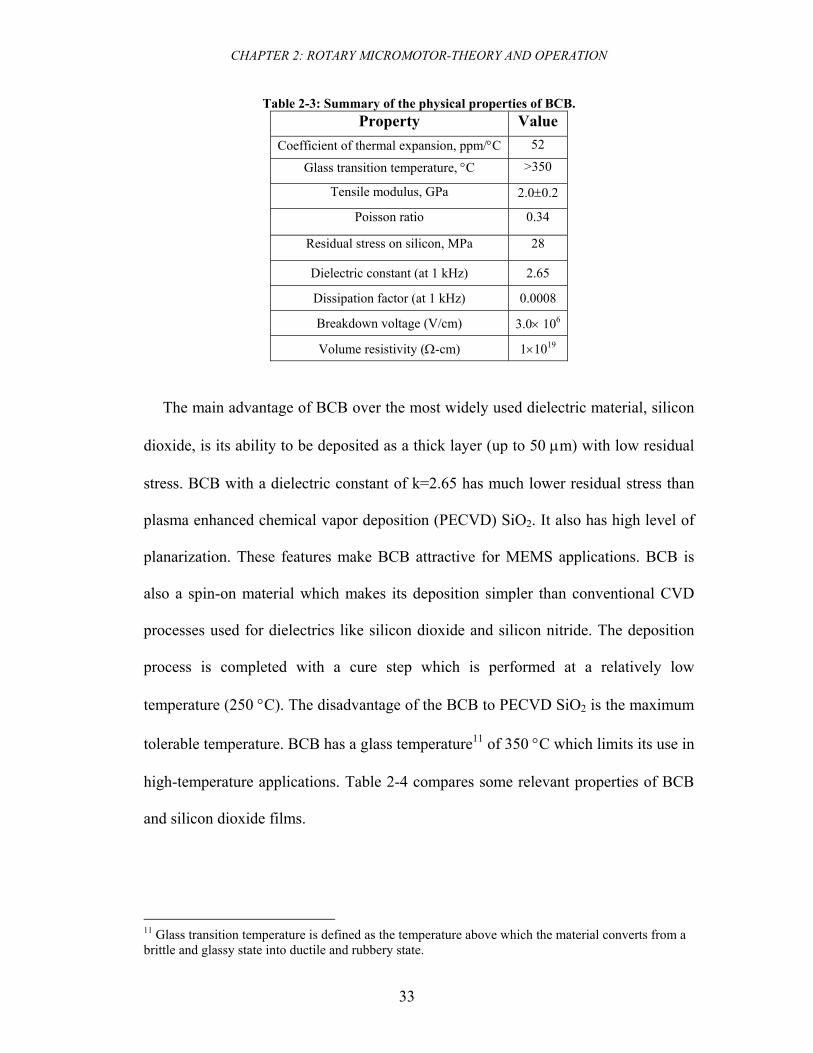
2.3 BCB-Based MEMS Technology
Spin-on, low dielectric constant BCB polymers [95-97] are promising candidates
as insulating dielectric material in MEMS. The electrical and mechanical properties
of this film are summarized in Table 2-3 [98].
Cyclotene is the commercial name of BCB produced by Dow Chemical Company
(Midland, MI) and is commercially available in different types and viscosities. In this
thesis the Cyclotene 3022 series was used in all the experiments. In this manuscript
the terms “BCB” and “Cyclotene” are used interchangeably despite the fact that BCB
refers to the chemical name of the monomer and Cyclotene carries the brand name.
CHAPTER 2: ROTARY MICROMOTOR-THEORY AND OPERATION
33
Table 2-3: Summary of the physical properties of BCB. Property Value
Coefficient of thermal expansion, ppm/°C 52
Glass transition temperature, °C >350
Tensile modulus, GPa 2.0±0.2
Poisson ratio 0.34
Residual stress on silicon, MPa 28
Dielectric constant (at 1 kHz) 2.65
Dissipation factor (at 1 kHz) 0.0008
Breakdown voltage (V/cm) 3.0× 10⁶
Volume resistivity (Ω-cm) 1×10¹⁹
The main advantage of BCB over the most widely used dielectric material, silicon
dioxide, is its ability to be deposited as a thick layer (up to 50 μm) with low residual
stress. BCB with a dielectric constant of k=2.65 has much lower residual stress than
plasma enhanced chemical vapor deposition (PECVD) SiO2. It also has high level of
planarization. These features make BCB attractive for MEMS applications. BCB is
also a spin-on material which makes its deposition simpler than conventional CVD
processes used for dielectrics like silicon dioxide and silicon nitride. The deposition
process is completed with a cure step which is performed at a relatively low
temperature (250 °C). The disadvantage of the BCB to PECVD SiO2 is the maximum
tolerable temperature. BCB has a glass temperature11 of 350 °C which limits its use in
high-temperature applications. Table 2-4 compares some relevant properties of BCB
and silicon dioxide films.
11 Glass transition temperature is defined as the temperature above which the material converts from a brittle and glassy state into ductile and rubbery state.
CHAPTER 2: ROTARY MICROMOTOR-THEORY AND OPERATION
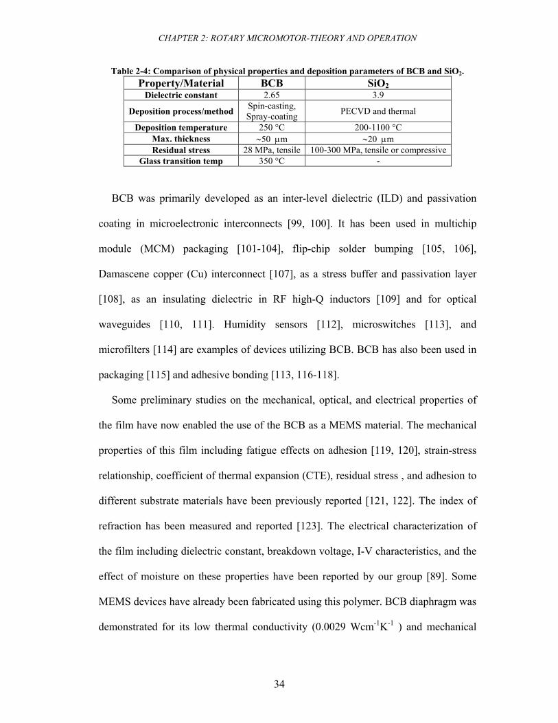
34
Table 2-4: Comparison of physical properties and deposition parameters of BCB and SiO2. Property/Material BCB SiO2
Dielectric constant 2.65 3.9
Deposition process/method Spin-casting, Spray-coating PECVD and thermal
Deposition temperature 250 °C 200-1100 °C Max. thickness ∼50 μm ∼20 μm Residual stress 28 MPa, tensile 100-300 MPa, tensile or compressive
Glass transition temp 350 °C -
BCB was primarily developed as an inter-level dielectric (ILD) and passivation
coating in microelectronic interconnects [99, 100]. It has been used in multichip
module (MCM) packaging [101-104], flip-chip solder bumping [105, 106],
Damascene copper (Cu) interconnect [107], as a stress buffer and passivation layer
[108], as an insulating dielectric in RF high-Q inductors [109] and for optical
waveguides [110, 111]. Humidity sensors [112], microswitches [113], and
microfilters [114] are examples of devices utilizing BCB. BCB has also been used in
packaging [115] and adhesive bonding [113, 116-118].
Some preliminary studies on the mechanical, optical, and electrical properties of
the film have now enabled the use of the BCB as a MEMS material. The mechanical
properties of this film including fatigue effects on adhesion [119, 120], strain-stress
relationship, coefficient of thermal expansion (CTE), residual stress , and adhesion to
different substrate materials have been previously reported [121, 122]. The index of
refraction has been measured and reported [123]. The electrical characterization of
the film including dielectric constant, breakdown voltage, I-V characteristics, and the
effect of moisture on these properties have been reported by our group [89]. Some
MEMS devices have already been fabricated using this polymer. BCB diaphragm was
demonstrated for its low thermal conductivity (0.0029 Wcm-1K-1 ) and mechanical
CHAPTER 2: ROTARY MICROMOTOR-THEORY AND OPERATION
35
robustness in a MEMS-based infra-red detector [124]. BCB has been also used for
fabricating single mode optical waveguides at 1300 nm [110]. Plane and curved
waveguide mirrors, the latter acting in the same way as cylindrical lenses, are made
with enhanced reflectivity by metallization of edges [111]. A red blood cell
microfilter was fabricated using BCB as a channel and bonding material [114]. In this
device blood cells are forced to pass through capillaries made out of BCB and glass
that are slightly smaller than their diameter. Healthy cells have enough deformability
to pass through the capillary. Chemical-mechanical planarization of BCB for both
integrated circuits and MEMS technology has been developed in the past few years
[125, 126].
In this dissertation, we have used BCB as interlayer dielectric, passivation, and
insulation layer due to its low permittivity and residual stress.
2.4 Theory of Micromachine Operation
2.4.1 Physics of Operation
The rotary variable-capacitance micromotor discussed here is a synchronous12
electrostatic machine. The stator (stationary part) is composed of a periodic structure
of metal conductors (electrodes) with a fixed spacing between them. The rotor
(movable part) is composed of a periodic salient silicon structure (poles), also with a
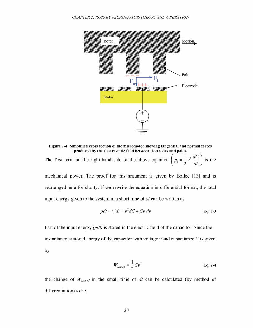
fixed spacing but different from that of the electrodes. Figure 2-4 shows the
simplified cross section of the device. If a potential is applied to an electrode, image
charges are induced on an adjacent pole. The resulting tangential and normal forces
are shown in Figure 2-4. The tangential force is the propelling force of the rotor 12 In the synchronous machines, unlike asynchronous (induction) counterparts, the mechanical motion of the rotor and electrical excitation of the stator are in sync i.e. follow one another.
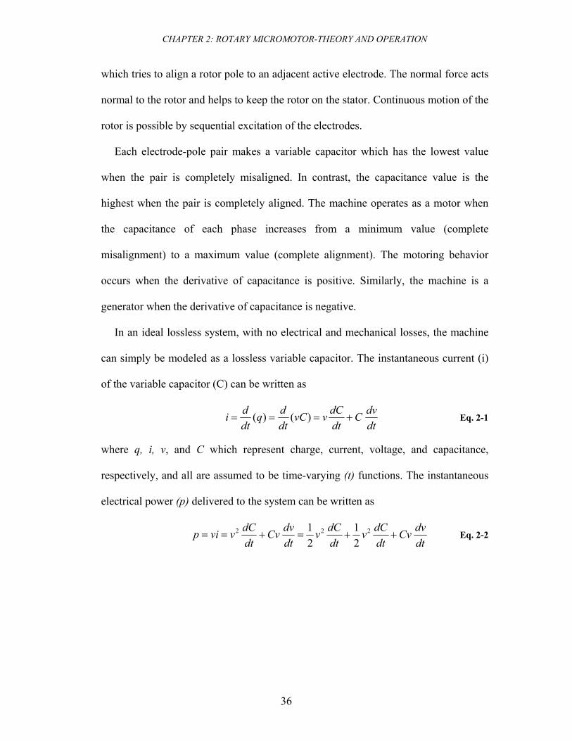
CHAPTER 2: ROTARY MICROMOTOR-THEORY AND OPERATION
36
which tries to align a rotor pole to an adjacent active electrode. The normal force acts
normal to the rotor and helps to keep the rotor on the stator. Continuous motion of the
rotor is possible by sequential excitation of the electrodes.
Each electrode-pole pair makes a variable capacitor which has the lowest value
when the pair is completely misaligned. In contrast, the capacitance value is the
highest when the pair is completely aligned. The machine operates as a motor when
the capacitance of each phase increases from a minimum value (complete
misalignment) to a maximum value (complete alignment). The motoring behavior
occurs when the derivative of capacitance is positive. Similarly, the machine is a
generator when the derivative of capacitance is negative.
In an ideal lossless system, with no electrical and mechanical losses, the machine
can simply be modeled as a lossless variable capacitor. The instantaneous current (i)
of the variable capacitor (C) can be written as
dtdvC
dtdCvvC
dtdq
dtdi +=== )()( Eq. 2-1
where q, i, v, and C which represent charge, current, voltage, and capacitance,
respectively, and all are assumed to be time-varying (t) functions. The instantaneous
electrical power (p) delivered to the system can be written as
dtdvCv
dtdCv
dtdCv
dtdvCv
dtdCvvip ++=+== 222
21
21
Eq. 2-2
CHAPTER 2: ROTARY MICROMOTOR-THEORY AND OPERATION
37
Figure 2-4: Simplified cross section of the micromotor showing tangential and normal forces produced by the electrostatic field between electrodes and poles.
The first term on the right-hand side of the above equation ⎟⎠⎞
⎜⎝⎛ =
dtdCvp 2
1 21 is the
mechanical power. The proof for this argument is given by Bollee [13] and is
rearranged here for clarity. If we rewrite the equation in differential format, the total
input energy given to the system in a short time of dt can be written as
dvCvdCvvidtpdt +== 2 Eq. 2-3
Part of the input energy (pdt) is stored in the electric field of the capacitor. Since the
instantaneous stored energy of the capacitor with voltage v and capacitance C is given
by
2
21 CvWStored = Eq. 2-4
the change of Wstored in the small time of dt can be calculated (by method of
differentiation) to be
+_
+++− − − FtFn
Rotor
Stator
Electrode
Pole
Motion
CHAPTER 2: ROTARY MICROMOTOR-THEORY AND OPERATION
38
CvdvdCvCvddWStored +=⎟⎠⎞
⎜⎝⎛= 22
21
21
Eq. 2-5
The remaining energy that is not stored in a loss-less system can be delivered to the
load as the mechanical energy,
dCvdWpdt Stored2
21
=− Eq. 2-6
Therefore, the mechanical power delivered to the load in an ideal lossless system is
dtdCvp 2
1 21
= Eq. 2-7
This power (p1) is due to the mechanical work, which must be performed by or on a
system at voltage v to change its capacitance at the rate of dtdC . The second and third
terms in the Eq. 2-3 are the stored power in the system. The term dtdCvp 2
2 21
=
represents the change in the stored energy of the electric field due to change in the
capacitance. The term dtdvCvp =3 represents the energy transferred from the external
power source (p) to the electrostatic field due to the change in the voltage (v).
When p2>0 the electric energy is being absorbed by the system and the mechanical
work is delivered. This state corresponds to a machine working as a motor. The motor
behavior is also shown Figure 2-4; the opposite charges on a single electrode-pole
attract each other and the rotor moves until the pair is aligned. In contrast, when p2<0
the mechanical energy is being absorbed by the system and the electrical work is
delivered. This state corresponds to a machine working as a generator. The sign of p2
is the same as dtdC . Therefore, assuming no phase difference between v2 and (dC/dt),
CHAPTER 2: ROTARY MICROMOTOR-THEORY AND OPERATION
39
one can conclude: dC/dt >0 corresponds to the motor state and (dC/dt)<0 corresponds
to the generator state. The above inequalities for the sign of (dC/dt) are only written
when an excitation voltage (v) is applied to the capacitor. Therefore, the regime in
which the machine operates depends on the sign of (dC/dt) and its interaction with
voltage (phase difference). For this reason, with correct excitation, the micromotor
can potentially be used as a microgenerator.
2.4.2 Role of Power Angle in Operation of the Machine
As mentioned above, the regime in which the machine operates depends on the
interaction of the excitation voltage and the mechanical movement (dC/dt). This
characteristic is expected from any synchronous machine. In order to illustrate the
effect of phase difference on the produced power, we assume that the capacitance and
excitation voltage have the simple forms of
)(sin)( 02 tCtC m ω= Eq. 2-8
)sin()( 0 φω += tVtv m Eq. 2-9
respectively; where ω0 is the angular frequency of the applied voltage and φ is the
phase difference between v(t) and C(t) (φ is also known as the power angle13). The
angular frequency (ω0) is chosen to be identical for both v(t) and C(t). This is a valid
assumption for any synchronous machine. C(t) is chosen to have a sinusoidal-squared
form with minimum and maximum of 0 and Cm , respectively14. To identify the role
13 The definition of power angle in other types of machines such as magnetic machines may differ from what is assumed here. No matter what definition is chosen, the result is the same. 14 Finite element analysis (FEA), discussed in Chapter 3, has proven that the choice of the sine-squared function for the capacitance is a valid.
CHAPTER 2: ROTARY MICROMOTOR-THEORY AND OPERATION
40
of phase difference (φ) on the produced electrical or mechanical power we derive
(dC/dt) as
)2sin()cos()sin(2)(00000 tCttC
dttdC
mm ωωωωω == Eq. 2-10
Figure 2-5 conceptualizes a variable-capacitance motor by plotting v2(t), C(t),
dC(t)/dt, and dtdCvp 2
1 21
= for a case where4πφ = . The average produced mechanical
power in one period, as shown in Figure 2-5, is positive; therefore, the machine
operates as a motor in this region ⎟⎠⎞
⎜⎝⎛ <<
20 πφ .
Power angle φ=0 corresponds to the generalized case when the average produced
mechanical power is zero. In this state, the machine is neither a motor nor a generator.
This case corresponds to the transitional point between the two regimes and is shown
in Figure 2-6. Similarly, when 02
<<πφ the machine is a generator with negative
mean mechanical power as shown in Figure 2-7 for 4πφ −= .
The last three figures show the relationship between power, voltage, and
capacitance at a three specific power angles. Thus, a more general case for the
produced power for a range of power angles is shown in Figure 2-8. The maximum
power in motoring mode is at φ=π/4. Similarly, at φ=-π/4 the maximum mechanical
power is consumed (generator).
To maximize the output power of the micromachine, one might use periodic
square-shape pulses (either positive or negative in amplitude) instead of the
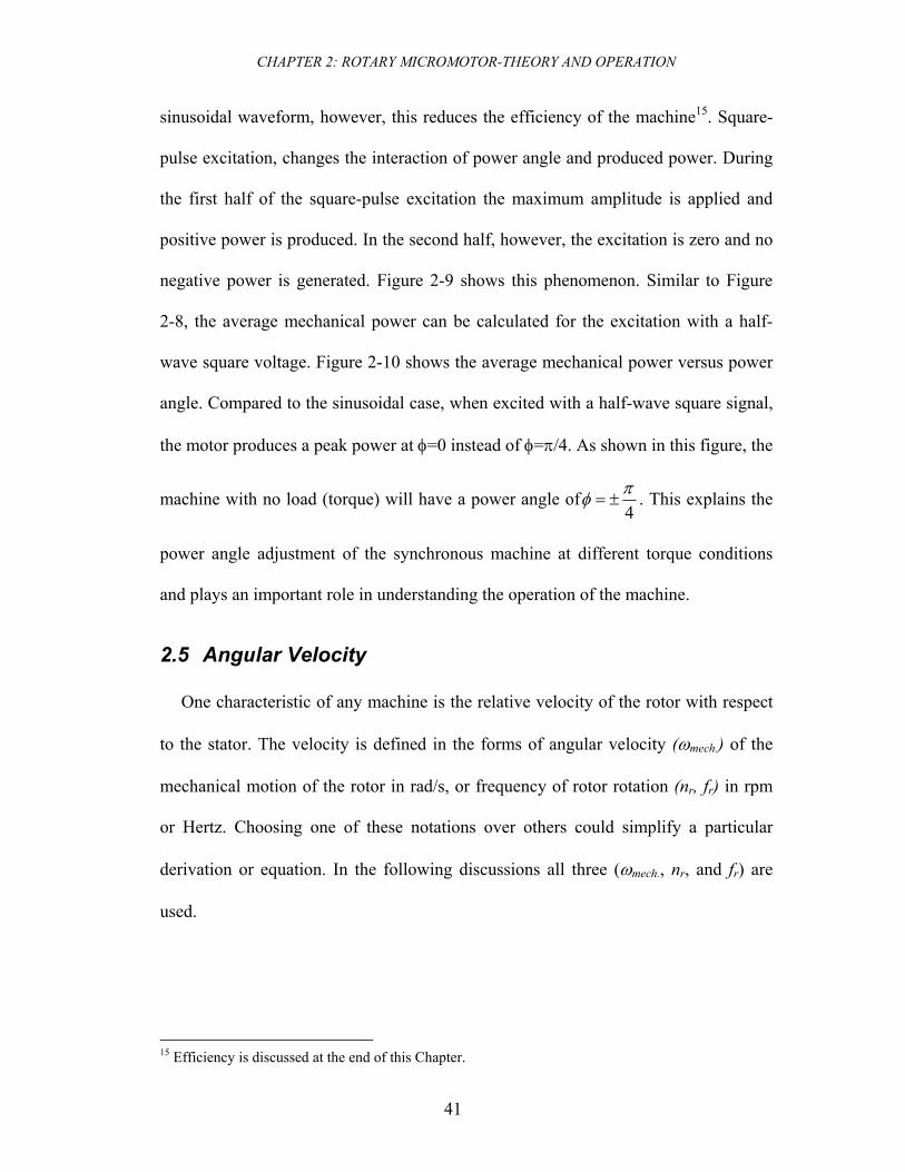
CHAPTER 2: ROTARY MICROMOTOR-THEORY AND OPERATION
41
sinusoidal waveform, however, this reduces the efficiency of the machine15. Square-
pulse excitation, changes the interaction of power angle and produced power. During
the first half of the square-pulse excitation the maximum amplitude is applied and
positive power is produced. In the second half, however, the excitation is zero and no
negative power is generated. Figure 2-9 shows this phenomenon. Similar to Figure
2-8, the average mechanical power can be calculated for the excitation with a half-
wave square voltage. Figure 2-10 shows the average mechanical power versus power
angle. Compared to the sinusoidal case, when excited with a half-wave square signal,
the motor produces a peak power at φ=0 instead of φ=π/4. As shown in this figure, the
machine with no load (torque) will have a power angle of4πφ ±= . This explains the
power angle adjustment of the synchronous machine at different torque conditions
and plays an important role in understanding the operation of the machine.
2.5 Angular Velocity
One characteristic of any machine is the relative velocity of the rotor with respect
to the stator. The velocity is defined in the forms of angular velocity (ωmech.) of the
mechanical motion of the rotor in rad/s, or frequency of rotor rotation (nr, fr) in rpm
or Hertz. Choosing one of these notations over others could simplify a particular
derivation or equation. In the following discussions all three (ωmech., nr, and fr) are
used.
15 Efficiency is discussed at the end of this Chapter.
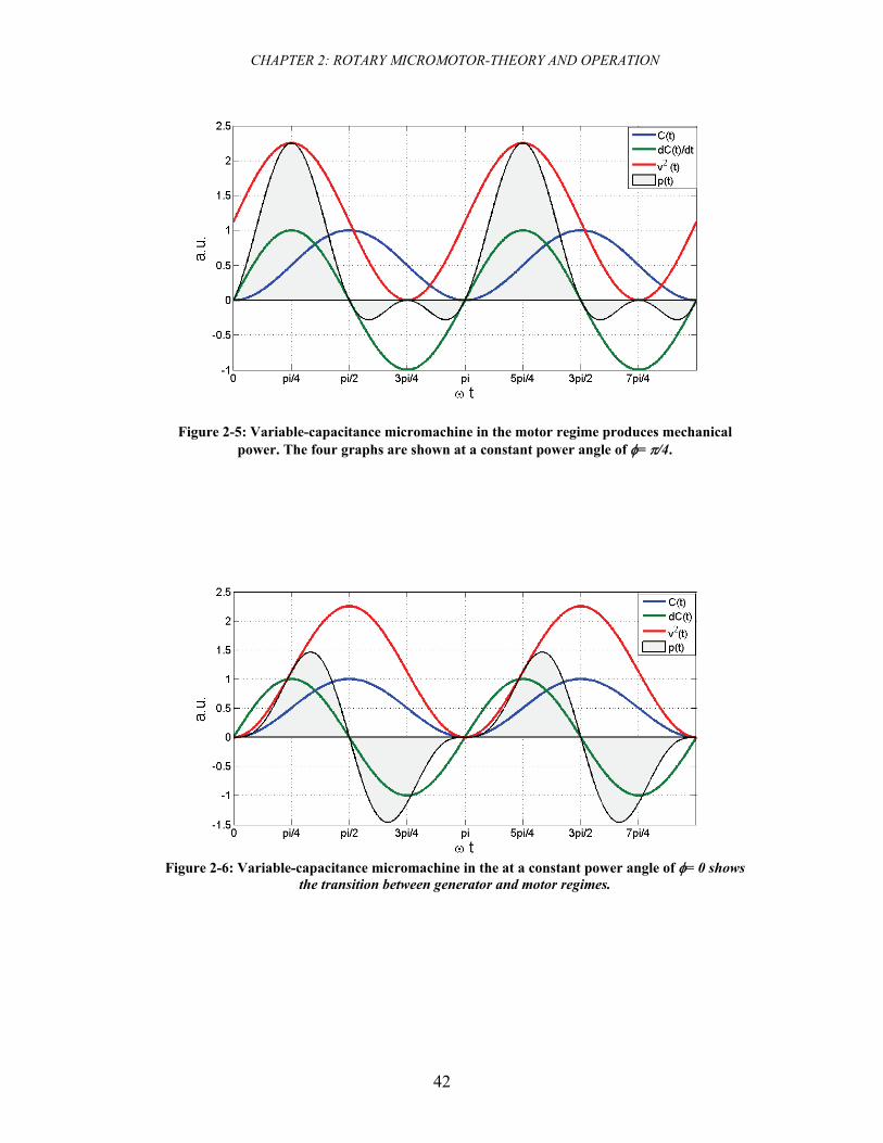
CHAPTER 2: ROTARY MICROMOTOR-THEORY AND OPERATION
42
Figure 2-5: Variable-capacitance micromachine in the motor regime produces mechanical power. The four graphs are shown at a constant power angle of φ= π/4.
Figure 2-6: Variable-capacitance micromachine in the at a constant power angle of φ= 0 shows
the transition between generator and motor regimes.
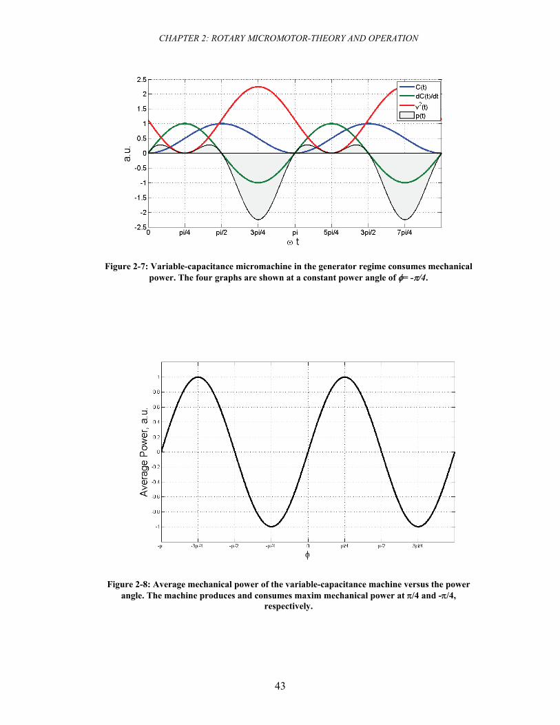
CHAPTER 2: ROTARY MICROMOTOR-THEORY AND OPERATION
43
Figure 2-7: Variable-capacitance micromachine in the generator regime consumes mechanical power. The four graphs are shown at a constant power angle of φ= -π/4.
Figure 2-8: Average mechanical power of the variable-capacitance machine versus the power angle. The machine produces and consumes maxim mechanical power at π/4 and -π/4,
respectively.
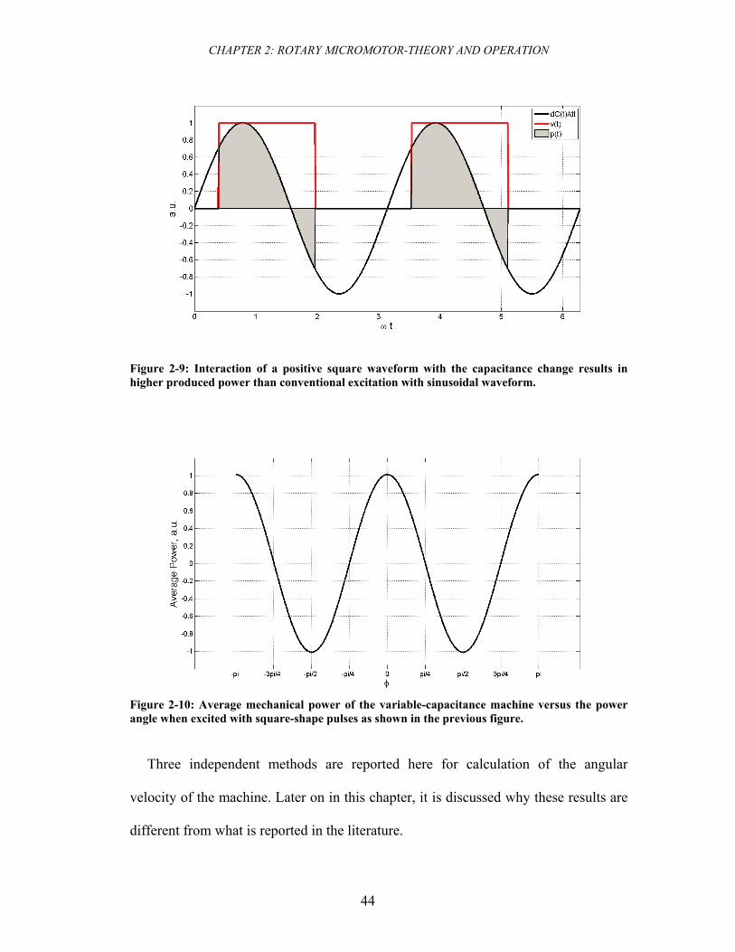
CHAPTER 2: ROTARY MICROMOTOR-THEORY AND OPERATION
44
Figure 2-9: Interaction of a positive square waveform with the capacitance change results in higher produced power than conventional excitation with sinusoidal waveform.
Figure 2-10: Average mechanical power of the variable-capacitance machine versus the power angle when excited with square-shape pulses as shown in the previous figure.
Three independent methods are reported here for calculation of the angular
velocity of the machine. Later on in this chapter, it is discussed why these results are
different from what is reported in the literature.
CHAPTER 2: ROTARY MICROMOTOR-THEORY AND OPERATION
45
2.5.1 Velocity from Linear Micromotor
The linear speed of the slider16 for a variable-capacitance machine, can be written
as
.2 elecr Wfu = Eq. 2-11
where ur is the linear speed of the slider in sm , W is the width of the electrode on the
stator in m, and felec. is the frequency of excitation voltage applied to the stator in Hz
[127]. This equation is based on the assumption that the spacing between two
adjacent poles equals their width (W). Assuming the period of Telec. for the excitation
voltage ( ).. 1 elecelec fT = , it is observed that if the mechanical motion of the slider is
synchronous with electrical excitation, the slider would move the linear distance
equal to the pole width (W) in a time equal to half of the period ( )2.elecT . A similar
formula can be applied to the rotary machine with some modifications described
below.
Using the linear mechanical speed and substituting the linear velocity with
equivalent angular velocity for a rotary machine results in
.. 2 elecmech Wfr =ω Eq. 2-12
where r is the radius of the circular rotor, and ωmech. is the angular velocity of the
rotor. Since rpm unit for speed is usually more practical, we can write ωmech. as a
function of nr using
rmech n602
.πω = Eq. 2-13
Therefore, 16 Slider refers to the moving part of the linear micromotor which is equivalent to the rotor for the rotary device.
CHAPTER 2: ROTARY MICROMOTOR-THEORY AND OPERATION
46
.2602
elecr Wfnr =π
Eq. 2-14
where nr is in rpm. Since for a rotary machine with Np number of poles
WN
r
p
22=
π Eq. 2-15
We can re-write
.2
602
elecp
r fN
rnr ππ= Eq. 2-16
Therefore,
p
elecr N
fn .60= Eq. 2-17
where nr is rotor mechanical speed in rpm, felec. is frequency of the electrical
excitation in Hz, and Np is the number of poles of the rotor. Similar to the linear
machine, the spacing between the poles of the rotary machine is assumed to be W.
The above equation describes the synchronization of electrical excitation voltage and
mechanical rotation of the rotor.
2.5.2 Velocity: Intuitive Method
It is also possible to derive the above equation without the use of linear machine
relations. If one were to stand on an electrode which is excited with a constant
frequency (felec.) and look at the poles of the machine, he/she will observe Np
complete capacitance charging cycles in each mechanical revolution. Therefore, one
electrical frequency is equal to pN1 mechanical angular frequency. As a result, the
mechanical angular speed (ωmech.) of the rotor, in synchronous with the electrical
angular frequency (ωelec.), is
CHAPTER 2: ROTARY MICROMOTOR-THEORY AND OPERATION
47
p
elecmech N
..
ωω = Eq. 2-18
With the same argument, the electrical angle (θelec.) and spatial angle (θmech.) of
the machine are related by the following expression
.. mechpelec N θθ = Eq. 2-19
The main characteristic of a synchronous machine is that the average mechanical
speed is only a function of the excitation frequency and the geometry of the machine.
Hence, with a given geometry, it is expected that a VCM operate at a constant speed
independent of the mechanical load conditions, as long as the excitation frequency is
kept constant.17
2.5.3 Velocity: Exact Method18
The synchronous angular velocity of the rotor also can be derived from electric
field theory. Assuming that the stator is excited with a 3-phase, square waveform with
a frequency of ω0 and phase difference of 2π/3, the instantaneous and position
dependent traveling potential (main harmonic only) on a single stator electrode
(without the presence of the rotor) is written as
( ) ( ) ( ) ( )υθωθϕ sinsin,, 0)1(
1 trCtr = Eq. 2-20
The superscript and subscript of ϕ denotes the phase number and harmonic number,
respectively, r and θ are the coordinates of the cylindrical system and υ is the number
of stator segments. In this approach the traveling potential which is a function of r, θ,
and t is written as a product of three functions. Each of these functions only depends 17 Constant velocity operation mode at different torques is only possible when the applied torque is not exceeding the maximum sustainable torque. 18 Derivation is rearranged based on the results of the personal communication with Professor Isaak Mayergoyz, University of Maryland (Dec 2006).
CHAPTER 2: ROTARY MICROMOTOR-THEORY AND OPERATION
48
on one variable only. C(r) is the radius-dependent function, sinω0t represents the 1st
harmonic of the electrical excitation signal and sinυθ represents the angular
dependency of the rotating potential.
Figure 2-11 shows the 2D simulation results of the electric field lines of the stator
with 4 electrodes without the presence of the rotor. Because in a variable capacitance
machine the gap is small and the rotor pole width is comparable to the stator width,
the traveling potential corresponding to the electric field line of Figure 2-11 is
perturbed with the presence of the bulky rotor. The perturbed field, shown in Figure
2-12, is now a function of the rotor position and has the position dependency of υ=Np
where Np is the number of “poles” on the rotor. Therefore, the modified potential for
a micromotor with presence of the rotor is
( ) ( ) ( ) ( )θωθϕ pNtrCtr sinsin,, 0)1(
1 = Eq. 2-21
Consequently, the potential for the second and third phases can be respectively
written as
( ) ( ) ⎟⎠⎞
⎜⎝⎛ −⎟
⎠⎞
⎜⎝⎛ −=
32sin
32sin,, 0
)2(1
πθπωθϕ pNtrCtr Eq. 2-22
( ) ( ) ⎟⎠⎞
⎜⎝⎛ −⎟
⎠⎞
⎜⎝⎛ −=
34sin
34sin,, 0
)3(1
πθπωθϕ pNtrCtr Eq. 2-23
The total instantaneous potential is simply the sum of all three potentials
( ) ( ) ( ) ( )trtrtrtr ,,,,,,,, )3(1
)2(1
)1(11 θϕθϕθϕθϕ ++= Eq. 2-24
( ) ( ) ( ) ( ) ( )
( ) ⎟⎠⎞
⎜⎝⎛ −⎟
⎠⎞
⎜⎝⎛ −
+⎟⎠⎞
⎜⎝⎛ −⎟
⎠⎞
⎜⎝⎛ −+=
34sin
34sin
32sin
32sinsinsin,,
0
001
πθπω
πθπωθωθϕ
p
pp
NtrC
NtrCNtrCtr
Eq. 2-25
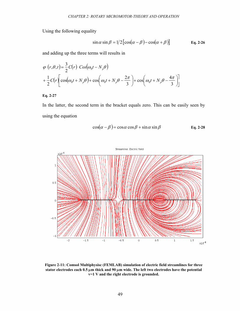
CHAPTER 2: ROTARY MICROMOTOR-THEORY AND OPERATION
49
Using the following equality
( ) ( )[ ]βαβαβα +−−= coscos21sinsin Eq. 2-26
and adding up the three terms will results in
( ) ( ) ( )
( ) ( ) ⎥⎦
⎤⎢⎣
⎡⎟⎠⎞
⎜⎝⎛ −++⎟
⎠⎞
⎜⎝⎛ −++++
−=
34cos
32coscos
21
23,,
000
0
πθωπθωθω
θωθϕ
ppp
p
NtNtNtrC
NtCosrCtr
Eq. 2-27
In the latter, the second term in the bracket equals zero. This can be easily seen by
using the equation
( ) βαβαβα sinsincoscoscos +=− Eq. 2-28
Figure 2-11: Comsol Multiphysisc (FEMLAB) simulation of electric field streamlines for three stator electrodes each 0.5 μm thick and 90 μm wide. The left two electrodes have the potential
v=1 V and the right electrode is grounded.
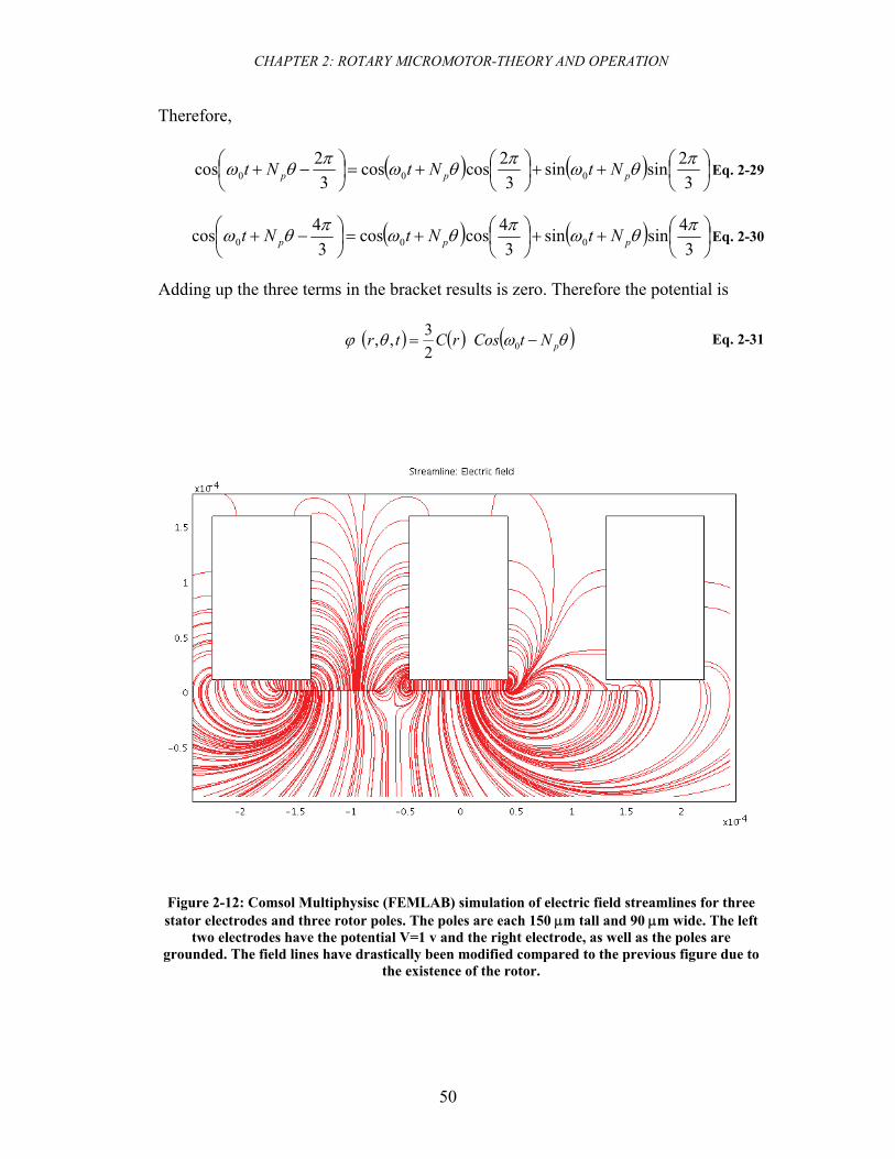
CHAPTER 2: ROTARY MICROMOTOR-THEORY AND OPERATION
50
Therefore,
( ) ( ) ⎟⎠⎞
⎜⎝⎛++⎟
⎠⎞
⎜⎝⎛+=⎟
⎠⎞
⎜⎝⎛ −+
32sinsin
32coscos
32cos 000
πθωπθωπθω ppp NtNtNt Eq. 2-29
( ) ( ) ⎟⎠⎞
⎜⎝⎛++⎟
⎠⎞
⎜⎝⎛+=⎟
⎠⎞
⎜⎝⎛ −+
34sinsin
34coscos
34cos 000
πθωπθωπθω ppp NtNtNt Eq. 2-30
Adding up the three terms in the bracket results is zero. Therefore the potential is
( ) ( ) ( )θωθϕ pNtCosrCtr −= 023,, Eq. 2-31
Figure 2-12: Comsol Multiphysisc (FEMLAB) simulation of electric field streamlines for three stator electrodes and three rotor poles. The poles are each 150 μm tall and 90 μm wide. The left
two electrodes have the potential V=1 v and the right electrode, as well as the poles are grounded. The field lines have drastically been modified compared to the previous figure due to
the existence of the rotor.
CHAPTER 2: ROTARY MICROMOTOR-THEORY AND OPERATION
51
In order to satisfy the condition of synchronization, the second term in the above
equation must be constant. For an observer traveling in synch with the traveling
potential, there should be no change in the amplitude of potential. As long as the
observer travels azimuthally with a constant radius we can write
( )( ) ConsttNtCos p =− θω0 Eq. 2-32
( ) ConsttNt p =− θω0 Eq. 2-33
By differentiating two sides of the equation
( )( ) 00 =− tNtdtd
pθω Eq. 2-34
( ) 00 =−dt
tdN pθω Eq. 2-35
The value ( )dt
tdθ is the angular velocity of the rotor. Therefore, the synchronous
angular velocity ωsynch. can be written as
( )p
synch Ndttd 0
.ωθω == Eq. 2-36
or
psynch N
f0.
2πω = Eq. 2-37
The angular rotor velocity in rpm is
pr N
fn 060= Eq. 2-38
2.5.4 Magnetic Versus Electrostatic
The speed of a variable-capacitance machine is often mistaken from the equation
describing the speed of magnetic synchronous machines (inaccurate expression is
CHAPTER 2: ROTARY MICROMOTOR-THEORY AND OPERATION
52
given by Trump [14]). The discrepancy originates from the definition of a pole. In a
magnetic machine, a pair of poles (N-S) makes the complete magnetic flux circuit;
therefore, there are Np/2 pairs in a machine. A single pole pair (N-S) is equivalent to
2π electrical radians. The electrical angle (θelec.) and the spatial angle (θmech.) of a
magnetic machine have the following relationship
.. 2 mechp
machinemagneticelec
Nθθ ⎟⎟⎠
⎞⎜⎜⎝
⎛= Eq. 2-39
The difference between the speed of a magnetic and electrostatic machine is the
factor of 21 for Np. The more elaborate comparison was provided in the previous
section when υ=Np for a variable-capacitance machine and υ=Np/2 for the magnetic
counterparts.
2.6 Torque and Mechanical Power
Torque is a fundamental machine property that needs to be evaluated. The
derivation of instantaneous and average torque of the machine is presented in this
section. The body of the rotor is considered to rotate about the z-axis where z is the
direction normal to the electrode surface (r, θ, and z are cylindrical coordinates). For
a small angular displacement (dθ ) the mechanical work performed by (or on) the
rotor is
θdTdW −=* Eq. 2-40
where W* is co-energy of a single capacitor and T is torque about the z-axis. The co-
energy is defined as
)()(* qWvqvW −= Eq. 2-41
CHAPTER 2: ROTARY MICROMOTOR-THEORY AND OPERATION
53
where q is the charge of the capacitor C(θ ) in coulombs, and W(q) is the stored
potential energy in the capacitor in Joules. The co-energy function is given by [128]
( ) ( ) 2*
21, vCvW θθ = Eq. 2-42
Torque (T) produced by a single variable-capacitor can also be written in a form of
tconsvvWT tan
* ),(=∂
∂−=
θθ
Eq. 2-43
where v is the applied voltage and considered to be constant and θ is defined in
counterclockwise angle from the x-axis. Therefore, the torque produced in a rotary
machine with a single capacitor is
( ) ( )θθ
θθθ
∂∂
−=∂
∂−= =
CvvWvT tconsv2
tan
*
21),(, Eq. 2-44
or the torque produced by an electrode-pole pair with capacitance C1
( ) ( )θθ
θ∂
∂−= 12
1 21,
CvvT Eq. 2-45
Assuming that the stator electrodes of the machine are excited in a six-phase
configuration where three phases are excited with positive square pulses (each 2π/3
apart) and the other three are excited identical to the first except with inverse
amplitude, the torque produced by each group of phases, or each “sector”, consisting
of 6eN electrodes will be
( ) ( ) ( )θθθθ
∂∂
−== 1211sec 2
16
,6
, CvNvTNvT eetor Eq. 2-46
where ( )θ,1sec vT tor is the total torque from similar phases (e.g. Phase A) of the
machine, Ne is number of electrodes on the stator, and C1 is the capacitance of one
particular phase. Geometrical symmetry of the machine suggests
CHAPTER 2: ROTARY MICROMOTOR-THEORY AND OPERATION
54
θθ ∂∂
=∂∂ +3nn CC
Eq. 2-47
where n is 1, 2, or 3. Excitation voltage is also symmetric (two of six phases are
excited identical with inverse amplitudes). Therefore,
( ) ( )θθ ,, 4sec1sec vTvT tortor = Eq. 2-48
( ) ( )θθ ,, 5sec2sec vTvT tortor = Eq. 2-49
( ) ( )θθ ,, 6sec3sec vTvT tortor = Eq. 2-50
The total torque of the machine can be written as
( ) ( ) ( ) ( ) ( ) ( ) ( )θθθθθθθ ,,,,,,, 6sec5sec4sec3sec2sec1sec vTvTvTvTvTvTvT tortortortortortor +++++=′Eq. 2-51
( ) ( ) ( ) ( )θθθθ ,2,2,2, 3sec2sec1sec vTvTvTvT tortortor ++=′ Eq. 2-52
The above equation is based on the assumption that at each time (t=t1) all the
electrode-pole pairs produce torque. This is not valid for a real machine. Assuming
64=ep NN for a 6:4 machine, at t=t1 either 2 or 4 pairs are active and participate in
producing torque. Therefore, on average ½ of the electrode-pole pairs are not excited.
Total torque of the machine can be written as
( ) ( )θθ ,21, vTvT ′= Eq. 2-53
( ) ( ) ( ) ( )θθθθ ,,,, 3sec2sec1sec vTvTvTvT tortortor ++= Eq. 2-54
( ) ( ) ( ) ( )⎥⎦⎤
⎢⎣⎡
∂∂
+∂
∂+
∂∂
−=θθ
θθ
θθ
θ 322212
21
621
621
6,
Cv
NCvNCv
NvT eee Eq. 2-55
( ) ( ) ( ) ( )⎟⎠⎞
⎜⎝⎛
∂∂
+∂
∂+
∂∂−
=θθ
θθ
θθθ 3212
121, CCCvNvT e Eq. 2-56
In above equation, v is given in volts (V), ( )( )θθ
∂∂C in
radF , and torque in N.m.
CHAPTER 2: ROTARY MICROMOTOR-THEORY AND OPERATION
55
Torque can be analytically evaluated if ( )θθ
∂∂ nC
values are known. Finite element
method (FEM) is used19 to simulate ( )θC and derive( )θθ
∂∂ nC
. The average total
torque for the six-phase machine can be calculated by integration:
( )⎥⎥⎥
⎦
⎤
⎢⎢⎢
⎣
⎡
⎟⎠⎞
⎜⎝⎛ ++⎟
⎠⎞
⎜⎝⎛ ++⎟
⎠⎞
⎜⎝⎛ −+= ∫∫∫∫
3
0
2
34
35
320
max
32sin
32sin
32sinsin
2
ππ
π
π
π
π πωπωπωωπ
ttttT
T total Eq. 2-57
where Tmax is the amplitude of a single-phase torque. As a result,
( ) ( ) ⎥⎦
⎤⎢⎣
⎡⎟⎠⎞
⎜⎝⎛ −+⎟
⎠⎞
⎜⎝⎛ −+−+−
−=
32coscos2cos
32cos0coscos0coscos
2max πππππππ
TT total
Eq. 2-58
[ ]62
max −−
=π
TT total Eq. 2-59
maxmax 9549.0
3T
TT total ==
π Eq. 2-60
Figure 2-13 shows the theoretical toque of each phase, as well as the total
instantaneous torque which is the sum of all phases.
19 Finite element analysis of ( )θC is discussed in Chapter 3.
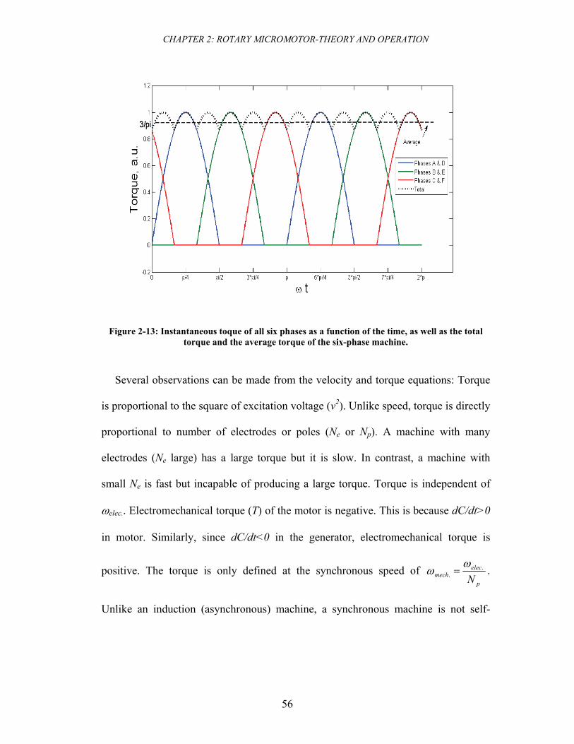
CHAPTER 2: ROTARY MICROMOTOR-THEORY AND OPERATION
56
Figure 2-13: Instantaneous toque of all six phases as a function of the time, as well as the total torque and the average torque of the six-phase machine.
Several observations can be made from the velocity and torque equations: Torque
is proportional to the square of excitation voltage (v2). Unlike speed, torque is directly
proportional to number of electrodes or poles (Ne or Np). A machine with many
electrodes (Ne large) has a large torque but it is slow. In contrast, a machine with
small Ne is fast but incapable of producing a large torque. Torque is independent of
ωelec.. Electromechanical torque (T) of the motor is negative. This is because dC/dt>0
in motor. Similarly, since dC/dt<0 in the generator, electromechanical torque is
positive. The torque is only defined at the synchronous speed of p
elecmech N
..
ωω = .
Unlike an induction (asynchronous) machine, a synchronous machine is not self-
CHAPTER 2: ROTARY MICROMOTOR-THEORY AND OPERATION
57
starting20. Due to the synchronization in variable-capacitance machines, the
successful starting from zero speed to the synch speed depends on the position of the
rotor, as well as phase and frequency of the applied voltage. External mechanical start
of the motor may be necessary in some cases. In practice ( )θθ
∂∂ nC
is not independent
of Ne. In a rotary machine Ne (or Np) is a function of the electrode (or pole) width, the
spacing between them, and the radius of the machine. Changing the parameters will
change Ne and ( )θC . However, Increasing Ne may result in decrease in ( )θθ
∂∂ nC
.
Therefore, choosing large Ne for obtaining large T is not always a preferred approach.
This issue is studied in Chapter 3.
Once the torque of the machine is derived, the output (input) mechanical power of
the motor (generator) can be given as
),(),( . θωθ vTvP mech−= Eq. 2-61
Substituting mechanical angular velocity with electrical angular frequency in the
above equation usingp
elecmech N
..
ωω = results in
),(),( . θωθ vTN
vPp
elec−= Eq. 2-62
By substitution
( ) ( ) ( )⎟⎠⎞
⎜⎝⎛
∂∂
+∂
∂+
∂∂
=θθ
θθ
θθω
θ 3212.
121),(
CCCvNN
vP ep
elec Eq. 2-63
( ) ( ) ( )⎟⎠⎞
⎜⎝⎛
∂∂
+∂
∂+
∂∂
=θθ
θθ
θθ
ωθ 3212.12
1),(CCC
vNN
vP elecp
e Eq. 2-64
20 An induction machine produces non-zero torque at zero speed, maximum torque at speeds less than ωmech, and zero torque at synchronous speed.
CHAPTER 2: ROTARY MICROMOTOR-THEORY AND OPERATION
58
The above equation can be further simplified assuming 64=ep NN ,
( ) ( ) ( )⎟⎠⎞
⎜⎝⎛
∂∂
+∂
∂+
∂∂
=θθ
θθ
θθ
ωθ 3212.4
6.121),(
CCCvvP elec Eq. 2-65
( ) ( ) ( )⎟⎠⎞
⎜⎝⎛
∂∂
+∂
∂+
∂∂
=θθ
θθ
θθ
ωθ 3212.8
1),(CCCvvP elec Eq. 2-66
It can be seen that the mechanical power is proportional to ωelec., voltage-squared, and
derivative of capacitance and independent of number of electrodes.
2.7 Power Generation
In the previous sections, the velocity of the machine, electromechanical torque,
and mechanical power were derived. We may consider the same device being used as
a microgenerator. In this case, the electrical output of the generator is of great
importance and is discussed here. The results from this discussion are insightful to the
micromotor and are used for evaluating two different modes of operation of the
micromotor as well as analyzing efficiency. For simplicity, the non-ideal effects like
electrical and mechanical losses are neglected in this section21. The electric power for
a lossless variable-capacitance machine can be derived from charge-voltage (Q-V)
behavior of the machine during different work cycles. Figure 2-14 shows these work
cycles for the motor and generator, respectively. A variable capacitor, C(θ), with a
voltage V and charge VCQ )(θ= and maximum and minimum of Cmax and Cmin is
considered in this case. When running a machine as a motor, path ABCA from Figure
2-14 is taken. Capacitor Cmin is first charged with a voltage source to voltage V0. The
capacitor charge at point B is
21 Non-ideal effects are discussed in the next section.
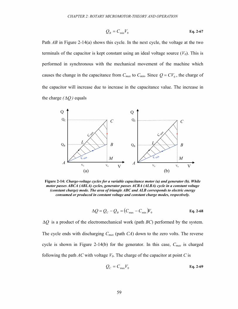
CHAPTER 2: ROTARY MICROMOTOR-THEORY AND OPERATION
59
0minVCQB = Eq. 2-67
Path AB in Figure 2-14(a) shows this cycle. In the next cycle, the voltage at the two
terminals of the capacitor is kept constant using an ideal voltage source (V0). This is
performed in synchronous with the mechanical movement of the machine which
causes the change in the capacitance from Cmax to Cmin. Since 0CVQ = , the charge of
the capacitor will increase due to increase in the capacitance value. The increase in
the charge ( QΔ ) equals
Figure 2-14: Charge-voltage cycles for a variable capacitance motor (a) and generator (b). While motor passes ABCA (ABLA) cycles, generator passes ACBA (ALBA) cycle in a constant voltage
(constant charge) mode. The area of triangle ABC and ALB corresponds to electric energy consumed or produced in constant voltage and constant charge modes, respectively.
( ) 0minmax VCCQQQ BC −=−=Δ Eq. 2-68
QΔ is a product of the electromechanical work (path BC) performed by the system.
The cycle ends with discharging Cmax (path CA) down to the zero volts. The reverse
cycle is shown in Figure 2-14(b) for the generator. In this case, Cmax is charged
following the path AC with voltage V0. The charge of the capacitor at point C is
0maxVCQC = Eq. 2-69
VS
MM
LLQB
QC
V
Q
A
B
V0
C
QB
QC
V
Q
A
B
V0
C
C max
C maxCmin Cmin
VS
(a) (b)
CHAPTER 2: ROTARY MICROMOTOR-THEORY AND OPERATION
60
The voltage is kept constant (path CB) at V0 while the capacitance drops from Cmax to
Cmin. The new charge on the capacitor is then QB . This is the electromechanical work
cycle where external mechanical force performs work using electric field. Cmin is
discharged into an external energy tank (reservoir) down to zero volts (path BA)22.
While the motor passes path ABCA, the generator passes path ACBA. This mode of
operation is called constant voltage, because the voltage of the variable capacitor is
externally kept constant using a voltage source. This mode can be used for both motor
and generator; however, due to complexity of drive circuits used for charging and
discharging the capacitor in generator-mode, it is preferred to run the generator in
another mode called constant charge. This mode can also be used for the motor;
however, drive circuit for motor is not as simple as constant voltage mode. The
constant charge path is shown in Figure 2-14(a) and (b) as paths of ABLA and ALBA,
respectively. The fundamental difference is that BC (CB) is replaced with BL (LB).
During this period, the charge of the capacitor (instead of voltage) is kept constant.
This can be accomplished by opening any circuit connected to the capacitor using a
switch. The advantage of this mode to the constant voltage mode is that there is no
need for using high-voltage source (V0) during electromechanical cycle. This
simplifies the drive requirements of the system. One can use the Figure 2-14 to derive
the electric energy and power. The slope of the AC and AB illustrates Cmax and Cmin,
respectively. Therefore,
AMCMC =max Eq. 2-70
22 In practice the time constant of the mechanical cycle (Cmin to Cmax or reverse) is much larger than the time constant of electrical cycles i.e. chare and discharging of the capacitor.
CHAPTER 2: ROTARY MICROMOTOR-THEORY AND OPERATION
61
AMBMC =min Eq. 2-71
Subtracting two values results in
AMCB
AMBM
AMCMCC =−=− minmax Eq. 2-72
By rearranging the above equation
( ) ( )minmax0minmax CCVCCAMCB −=−= Eq. 2-73
where 0VAM = . The electrical power can be calculated using Figure 2-14. The
energy stored in the system is
∫= dVQE Eq. 2-74
where E is the electrical energy in Joules. The area of triangles ABC and ABL defines
the electrical energy in constant voltage (Evoltage) and constant charge (Echarge) modes,
respectively. These areas are equal to
( ) 20minmax2
121 VCCAMCBSE ABCvoltage −=== Δ Eq. 2-75
Therefore, the energy in the voltage constant mode is
( ) 20minmax2
1 VCCEvoltage −= Eq. 2-76
Similarly, in the constant-charge mode we have
ΔΔΔ −== BCLABCABLech SSSE arg ( ) ⎥⎦⎤
⎢⎣⎡−⎥⎦
⎤⎢⎣⎡ −= BLCBVCCE ech 2
121 2
0minmaxarg Eq. 2-77
Replacing CB and BL using ( )minmax0 CCVCB −= and sVVBL −= 0 results in
( ) ( )( ) ( )⎥⎦⎤
⎢⎣⎡ −−−⎥⎦
⎤⎢⎣⎡ −= sech VVCCVVCCE 0minmax0
20minmaxarg 2
121
Eq. 2-78
CHAPTER 2: ROTARY MICROMOTOR-THEORY AND OPERATION
62
( ) sech VVCCE 0minmaxarg 21
−= Eq. 2-79
This equation can be further simplified. Using geometry shown in Figure 2-14 we can
write
sVV
CAM
CAM
ALAC
ALAC
BMCM
AMBMAMCM
CC 0
min
max
cos
cos=
⎟⎠⎞
⎜⎝⎛
⎟⎠⎞
⎜⎝⎛
====∧
∧
Eq. 2-80
Therefore, the charge constant energy can be further simplified as
( ) sech VVCCE 0minmaxarg 21
−= Eq. 2-81
( ) ssech VCC
VCCEmin
maxminmaxarg 2
1−= Eq. 2-82
( ) 2minmax
min
maxarg 2
1sech VCC
CCE −= Eq. 2-83
It is clear from Figure 2-14 that the energy produced in the constant voltage mode
is higher than the energy produced in the constant charge mode. The power of the
machine (motor and generator) can be calculated from energy relations. Assuming the
machine is rotating with mechanical frequency of fmech.(Hz), we can write the average
electric power to be
)21(.. epmechelec NNfEP = Eq. 2-84
where Pelec. is the average electric power in Watts and E is the energy in Joules. It was
mentioned earlier that in these types of machines during ½ of the time, 4 of 6 phases
are excited and during the other half only 2 of 6 phases are excited. Therefore, on
average, 2eN electrodes are excited and participate in electric power production. The
CHAPTER 2: ROTARY MICROMOTOR-THEORY AND OPERATION
63
Np term in the power equation counts for the fact that in each rotation a single excited
electrode passes by Np poles. The Ne term counts for all of the electrodes that are
excited in each rotation. Since
ep NN64
= Eq. 2-85
the power can be written as
)31( 2
.. emechelec NfEP = Eq. 2-86
In order to write the mechanical speed in rpm units we use
rmech nf6022 .ππ = Eq. 2-87
Substituting .mechf with rotation frequency in rpm unit ( rn ) results in
)31(
602
. er
elec NnEP = Eq. 2-88
2.
1801
erelec NnEP = Eq. 2-89
where Pelec. is in Watts, E in Joules, and nr in rpm. Substituting E with Echarge results
in
2arg.arg.
1801
erechconstechelec NnEP = Eq. 2-90
( ) 22minmax
min
max.arg.
21
1801
ersconstechelec NnVCCCCP −= Eq. 2-91
( ) 22minmax
min
max.arg.
3601
ersconstechelec NnVCCCCP −= Eq. 2-92
Electric power for constant voltage mode is similarly calculated to be
2..
1801
ervoltageconstvoltageelec NnEP = Eq. 2-93
CHAPTER 2: ROTARY MICROMOTOR-THEORY AND OPERATION
64
( ) 220minmax..
21
1801
erconstvoltageelec NnVCCP −= Eq. 2-94
( ) 220minmax..
3601
erconstvoltageelec NnVCCP −= Eq. 2-95
The two equations describing the power for two modes have two significant
differences. First, the power in the constant voltage mode is proportional to 20V ,
whereas, the power in constant charge equation is proportional to 2sV . Since 0VVs < ,
the power of constant charge mode is expected to be less than constant voltage mode.
Second, the term 1min
max >CC does not exist in the constant voltage equation.
2.8 Losses and Efficiency
A micromachine converts one form of energy to another i.e. electrical to
mechanical energy. This energy transduction is often accompanied with losses in the
system. Two types of losses are associated with the micromotor: mechanical and
electrical. Figure 2-15 shows the flow diagram of energy from the electrical input to
the mechanical output. Some electrical energy is lost in the form of heat in power
electronics, stator electrodes, and rotor conductors (poles). Frictional losses of rolling
and sliding bearings and viscous drag loss of a rotating disk are the major sources of
mechanical loss.
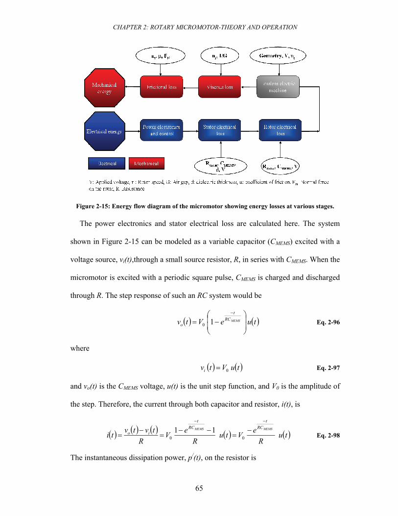
CHAPTER 2: ROTARY MICROMOTOR-THEORY AND OPERATION
65
Figure 2-15: Energy flow diagram of the micromotor showing energy losses at various stages.
The power electronics and stator electrical loss are calculated here. The system
shown in Figure 2-15 can be modeled as a variable capacitor (CMEMS) excited with a
voltage source, vi(t),through a small source resistor, R, in series with CMEMS. When the
micromotor is excited with a periodic square pulse, CMEMS is charged and discharged
through R. The step response of such an RC system would be
( ) ( )tueVtv MEMSRCt
o ⎟⎟⎠
⎞⎜⎜⎝
⎛−=
−
10 Eq. 2-96
where
( ) ( )tuVtvi 0= Eq. 2-97
and vo(t) is the CMEMS voltage, u(t) is the unit step function, and V0 is the amplitude of
the step. Therefore, the current through both capacitor and resistor, i(t), is
( ) ( ) ( ) ( ) ( )tuR
eVtuR
eVR
tvtvtiMEMSMEMS RC
tRC
t
io
−−
−=
−−=
−= 00
11 Eq. 2-98
The instantaneous dissipation power, p/(t), on the resistor is
CHAPTER 2: ROTARY MICROMOTOR-THEORY AND OPERATION
66
( ) ( ) ( )tuR
eVtiRtpMEMSRC
t2
20
2
−
==′ Eq. 2-99
The average power would be23
( ) ( ) ( ) MEMSMEMS
t
RCt
CVR
RCVdttuR
eVtpMEMS
20
20
0
2
20 2
11012
=−−
==′ ∫∞
=
−
Eq. 2-100
Therefore, the dissipated power is independent of the resistor size. Considering a
periodic square pulse, with a fixed frequency of f0 applied to a variable capacitor
CMin<CMEMS<CMax, the total average dissipated power would be
( ) ( )MaxMinMaxMinLoss CCVCVCVtp +=+= 20
20
20 2
121
21
Eq. 2-101
The above equation is written with the assumption that the charge and discharge of
the capacitor is occurred exactly when the capacitance is at minimum and maximum
values, respectively (motor). As shown in the previous section, the energy produced
in a constant-voltage cycle is
( ) 20minmax2
1 VCCEvoltage −= Eq. 2-102
And the average power is
( ) 02
0minmax21 fVCCPOut −= Eq. 2-103
Finally, the theoretical efficiency of the system is
⎟⎟⎠
⎞⎜⎜⎝
⎛−=
−=
+==
Max
Min
Max
MinMax
LossOut
Out
In
Out
CC
CCC
PPP
PP
121
2η Eq. 2-104
The maximum theoretical system efficiency is 50% for CMin=0.
23 CMEMS was treated as a constant when calculating the integral. This is a valid assumption since the RC time constant is orders of magnitude smaller than the period of the excitation signal.
CHAPTER 3: DESIGN AND SIMULATION
67
3 Design and Simulation
3.1 Introduction
The first step in designing the micromachine is to identify the relevant parameters,
i.e. input and output variables. The input design variables are geometrical features,
electrical, mechanical, material properties of components, and electrical excitation
schemes. The output variables are toque, angular velocity, and efficiency of the
machine. The relationship between output variables and input variables were derived
in Chapter 2. In this chapter, the detailed design methodology of the micromotor is
reported. First, geometric, electrical, mechanical, and material considerations are
discussed first. Next, finite element simulations used for modeling the effects of input
variables on the output variables. Several micromotors with different geometries are
the outcome of the study. Final design details are discussed and the output variables
are provided for each design. Finally, a CAD tool is used for drawing the geometries.
This step has been the most challenging part of the design due to the complexity of
the 9-level-mask layout.
3.2 Design Considerations and Limitations
The rotary micromotor, as discussed in Chapter 2, is composed of three
components: stator, rotor, and microballs. The microballs are available in a diameter
of φ=285.4 μm. The geometry of the stator and rotor are designed based on the
factors discussed in this section.
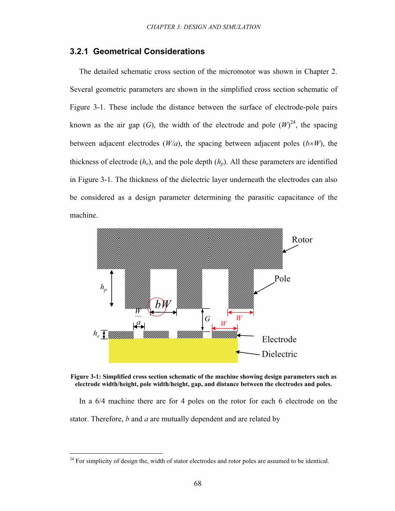
CHAPTER 3: DESIGN AND SIMULATION
68
3.2.1 Geometrical Considerations
The detailed schematic cross section of the micromotor was shown in Chapter 2.
Several geometric parameters are shown in the simplified cross section schematic of
Figure 3-1. These include the distance between the surface of electrode-pole pairs
known as the air gap (G), the width of the electrode and pole (W)24, the spacing
between adjacent electrodes (W/a), the spacing between adjacent poles (b×W), the
thickness of electrode (he), and the pole depth (hp). All these parameters are identified
in Figure 3-1. The thickness of the dielectric layer underneath the electrodes can also
be considered as a design parameter determining the parasitic capacitance of the
machine.
Rotor
Pole
ElectrodeDielectric
WWa
WbW
hp
he
G
Figure 3-1: Simplified cross section schematic of the machine showing design parameters such as electrode width/height, pole width/height, gap, and distance between the electrodes and poles.
In a 6/4 machine there are for 4 poles on the rotor for each 6 electrode on the
stator. Therefore, b and a are mutually dependent and are related by
24 For simplicity of design the, width of stator electrodes and rotor poles are assumed to be identical.
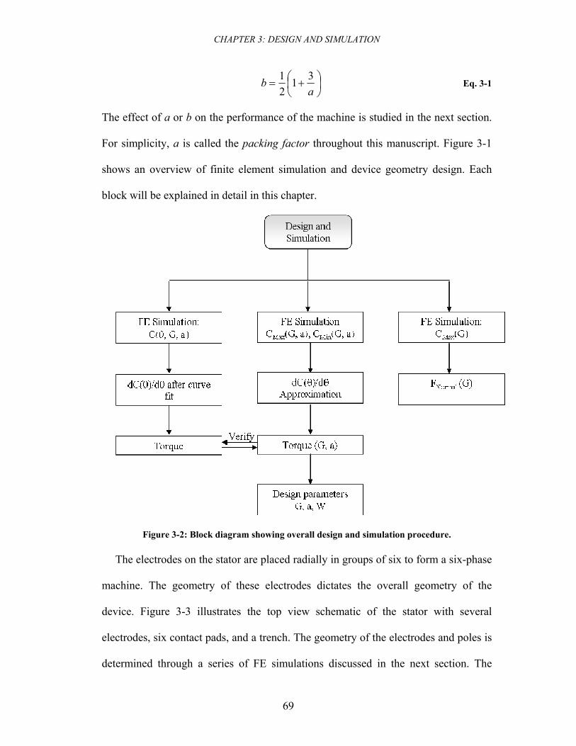
CHAPTER 3: DESIGN AND SIMULATION
69
⎟⎠⎞
⎜⎝⎛ +=
ab 31
21
Eq. 3-1
The effect of a or b on the performance of the machine is studied in the next section.
For simplicity, a is called the packing factor throughout this manuscript. Figure 3-1
shows an overview of finite element simulation and device geometry design. Each
block will be explained in detail in this chapter.
Figure 3-2: Block diagram showing overall design and simulation procedure.
The electrodes on the stator are placed radially in groups of six to form a six-phase
machine. The geometry of these electrodes dictates the overall geometry of the
device. Figure 3-3 illustrates the top view schematic of the stator with several
electrodes, six contact pads, and a trench. The geometry of the electrodes and poles is
determined through a series of FE simulations discussed in the next section. The
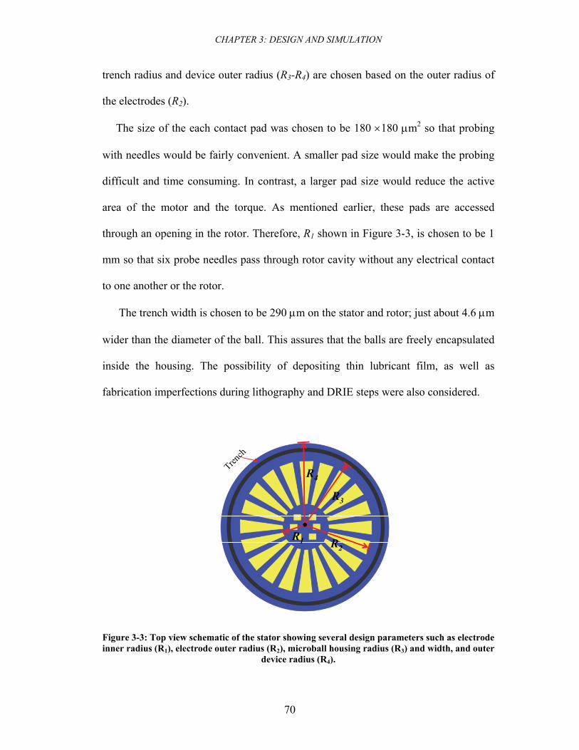
CHAPTER 3: DESIGN AND SIMULATION
70
trench radius and device outer radius (R3-R4) are chosen based on the outer radius of
the electrodes (R2).
The size of the each contact pad was chosen to be 180 ×180 μm2 so that probing
with needles would be fairly convenient. A smaller pad size would make the probing
difficult and time consuming. In contrast, a larger pad size would reduce the active
area of the motor and the torque. As mentioned earlier, these pads are accessed
through an opening in the rotor. Therefore, R1 shown in Figure 3-3, is chosen to be 1
mm so that six probe needles pass through rotor cavity without any electrical contact
to one another or the rotor.
The trench width is chosen to be 290 μm on the stator and rotor; just about 4.6 μm
wider than the diameter of the ball. This assures that the balls are freely encapsulated
inside the housing. The possibility of depositing thin lubricant film, as well as
fabrication imperfections during lithography and DRIE steps were also considered.
R4
R2R1
R3
Trench
Figure 3-3: Top view schematic of the stator showing several design parameters such as electrode inner radius (R1), electrode outer radius (R2), microball housing radius (R3) and width, and outer
device radius (R4).
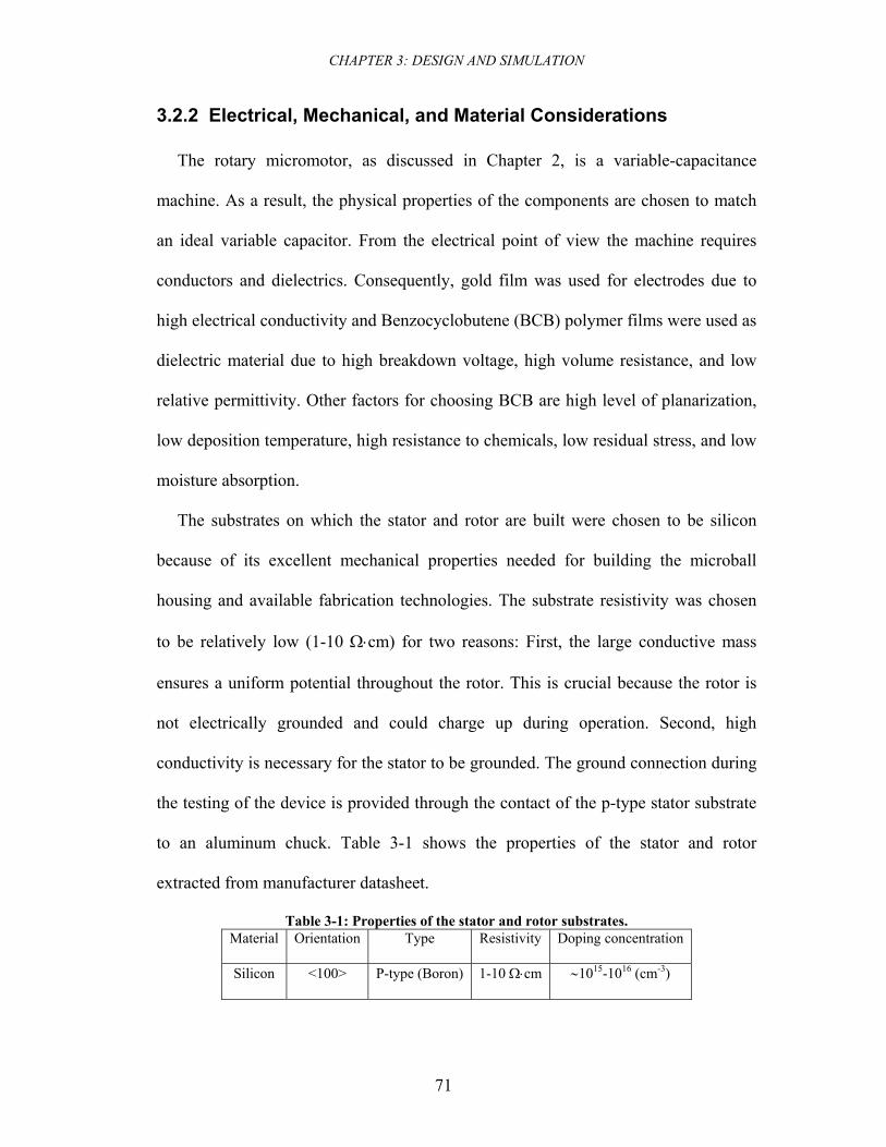
CHAPTER 3: DESIGN AND SIMULATION
71
3.2.2 Electrical, Mechanical, and Material Considerations
The rotary micromotor, as discussed in Chapter 2, is a variable-capacitance
machine. As a result, the physical properties of the components are chosen to match
an ideal variable capacitor. From the electrical point of view the machine requires
conductors and dielectrics. Consequently, gold film was used for electrodes due to
high electrical conductivity and Benzocyclobutene (BCB) polymer films were used as
dielectric material due to high breakdown voltage, high volume resistance, and low
relative permittivity. Other factors for choosing BCB are high level of planarization,
low deposition temperature, high resistance to chemicals, low residual stress, and low
moisture absorption.
The substrates on which the stator and rotor are built were chosen to be silicon
because of its excellent mechanical properties needed for building the microball
housing and available fabrication technologies. The substrate resistivity was chosen
to be relatively low (1-10 Ω⋅cm) for two reasons: First, the large conductive mass
ensures a uniform potential throughout the rotor. This is crucial because the rotor is
not electrically grounded and could charge up during operation. Second, high
conductivity is necessary for the stator to be grounded. The ground connection during
the testing of the device is provided through the contact of the p-type stator substrate
to an aluminum chuck. Table 3-1 shows the properties of the stator and rotor
extracted from manufacturer datasheet.
Table 3-1: Properties of the stator and rotor substrates. Material Orientation Type Resistivity Doping concentration
Silicon <100> P-type (Boron) 1-10 Ω⋅cm ∼1015-1016 (cm-3)
CHAPTER 3: DESIGN AND SIMULATION
72
3.3 Finite Element Simulation
3.3.1 Simulation Basics
In order to obtain accurate quantitative values for the capacitance of the system
through finite element method (FEM), one must consider the fundamental definition
for capacitance. The argument made here is also used in defining appropriate
boundary conditions for solving the problem.
For a system of n conductors, each with potential Vi and total charge Qi, the linear
functional dependence of the potential on the charge density implies that the potential
of the ith conductor be [129]
( )niQpVn
jJiji ,,2,1
1L==∑
=
Eq. 3-2
where pij depend on the geometry of the conductors. Inverting the above equation
results in
( )niVCQn
jjiji ,,2,1
1L==∑
=
Eq. 3-3
In the above equation, only the Cii coefficients are called capacitance25. For example
in a system of two conductors,
2221212 VCVCQ += Eq. 3-4
In order to obtain the C22 value, V1 is set to zero. Therefore, by definition “the
capacitance of the conductor is the total charge on the conductor when is maintained
at unit potential, all other conductors being held at zero potential” [129].
Consequently, in assigning the boundary conditions, only one electrode is set to have
25 Cij, i≠j, are called coefficients of induction!
CHAPTER 3: DESIGN AND SIMULATION
73
none-zero potential while the rest of the structure is set to 0 V. The potential energy
of a system with n conductors can be written as the product of charge and potential
j
n
i
n
jiiji
n
iie VVCVQW ∑∑∑
= ==
==1 11 2
121
Eq. 3-5
The Comosol Mutiphysics (FEMLAB) software was used in all the simulations
discussed in this chapter. The Poisson’s Equation is solved to obtain the potential V
using
( ) ρεε =∇∇− VR0 Eq. 3-6
where ρ is the space charge density, ε0 and εR are the permittivity of vacuum and
relative permittivity of the medium, respectively. The energy (We) is then calculated
by the software. With appropriate subdomain settings of V=0 and V=1 V the
capacitance is simply C=2We.
3.3.2 Modeling Sequence
The FE simulation is composed of four major steps. The first step is to define a
suitable geometry representing the actual structure of the micromotor. The second
step is to outline sub-domain and boundary conditions such that applicable material
properties, symmetric conditions, and physics of operation are represented. The third
step is to mesh the structure. This is a critical step since it affects the accuracy and
validity of the solution, as well as the time and complexity of numerical computation.
The last step is to solve the Poisson’s Equation using finite element method and
compute the total energy stored in the system (We).
CHAPTER 3: DESIGN AND SIMULATION
74
3.3.3 Sub-Domains and Boundary Conditions
Figure 3-4(a) shows the geometry used for simulating the capacitance versus
angular position of the rotor. Due to the lack of symmetry, a complete sector of the
machine consisting of 6 electrodes and 4 poles is simulated. Large number of high-
aspect-ratio electrodes (ratio of ∼10000) made this simulation extremely complex and
time consuming. Simulation results for C(θ) are reported and discussed later in this
chapter.
Symmetry of the micromotor at full alignment and misalignment allows further
simplification of the simulated geometry to 3 electrodes and 2 poles as shown in
Figure 3-4(b). The simplified structure is simulated to obtain maximum and minimum
capacitance and, consequently, the torque. A sample meshed structure is shown in
Figure 3-1(c) where near 300,000 elements were used. Meshing the high-aspect-ratio
geometry was challenging and was performed by increasing and decreasing the
number of mesh elements in the z and r directions26, respectively. In the first case
where 6 electrodes and 4 poles were simulated, about 600,000 mesh elements were
used and the problem had nearly 700,000 degrees of freedom27.
Figure 3-5 shows the boundary conditions used for the simulation of CMax and CMin
based on the discussion in Section 3.1.1. Except one electrode, all the structure is set
to be electrically grounded including the box representing the symmetrical boundary
conditions. Sample simulation results for the electric energy density and potential are
shown in Figure 3-6. In cases where the C(θ) is simulated a complete segment of the
26 z and r refer to cylindrical coordinates. 27 Generally for simplicity, 2D simulations are chosen over of 3D. However, to improve the accuracy and validity of our model a series of 3D simulations were performed in this study, despite the complexity of the problem.
CHAPTER 3: DESIGN AND SIMULATION
75
machine composed of 6 electrodes and 4 poles is used due to lack of symmetry. For
the torque simulation, however, the simplified geometry is used due to symmetry.
3.3.4 Effect of the Electrode Spacing and the Gap
The torque of the machine, being the most important output variable, was derived
in Chapter 2 as
( ) ( ) ( ) ( )⎟⎠⎞
⎜⎝⎛
∂∂
+∂
∂+
∂∂−
=θθ
θθ
θθθ 3212
121, CCCvNvT e Eq. 3-7
The above equation demonstrates that in order to design a machine with a high
torque, the product of Ne and dC/dθ must be maximized. One way to change this
product is to change the packing factor of the electrodes (a). First, at a fixed gap, the
dC/dθ value versus packing factor is calculated. The next step is to fix the packing
factor and vary the gap.
A variable capacitor with a gap of 10 μm and a packing factor of 3 was simulated.
The capacitance versus the angular position of the rotor is shown in Figure 3-7. This
graph is a result of 17 individual simulations with 6 electrodes and 4 rotors. The
summary of the geometrical values and assumptions used in the simulation is shown
in Figure 3-8. The figure shows the full cycle for each segment. As the rotor rotates,
the capacitor value changes from maximum (full alignment) to minimum (full
misalignment) and eventually to maximum (full alignment).
Figure 3-7 demonstrates the curve fit to the simulated data too. The capacitance
values are fitted to the sine-squared function in a form of
( )2
32
102sin ⎥
⎦
⎤⎢⎣
⎡⎟⎟⎠
⎞⎜⎜⎝
⎛++= a
aaCC πθθ Eq. 3-8
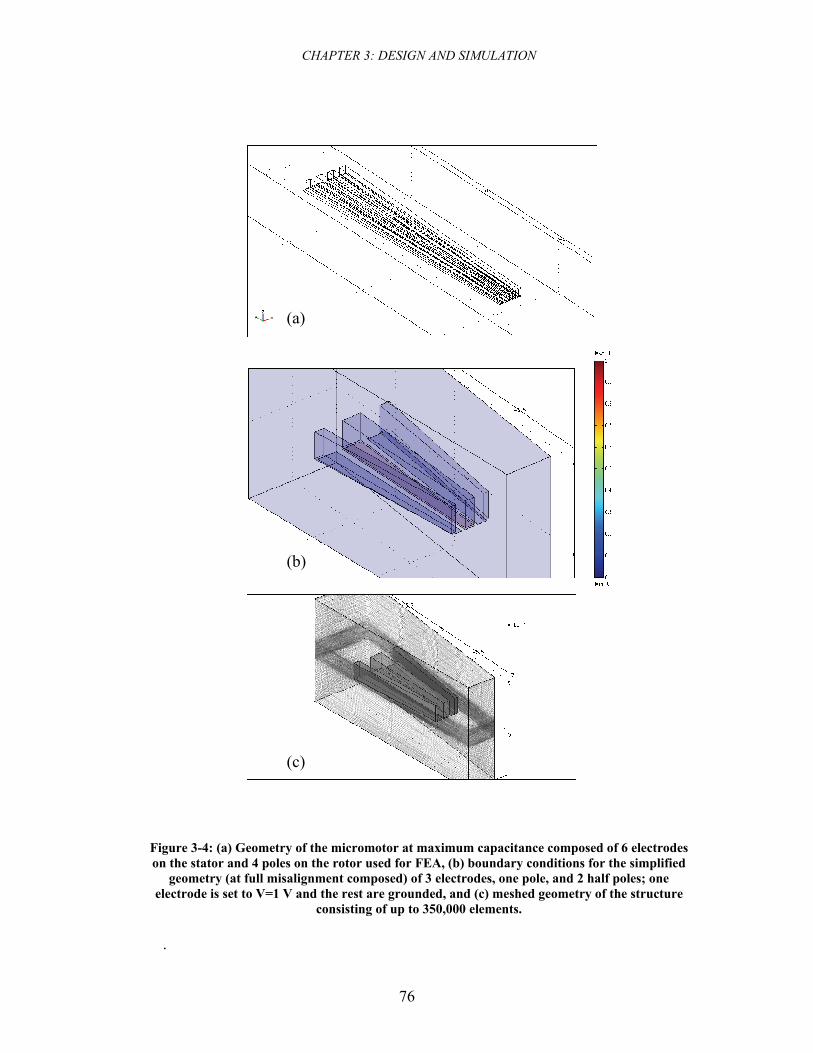
CHAPTER 3: DESIGN AND SIMULATION
76
(a)
(b)
(c)
Figure 3-4: (a) Geometry of the micromotor at maximum capacitance composed of 6 electrodes on the stator and 4 poles on the rotor used for FEA, (b) boundary conditions for the simplified
geometry (at full misalignment composed) of 3 electrodes, one pole, and 2 half poles; one electrode is set to V=1 V and the rest are grounded, and (c) meshed geometry of the structure
consisting of up to 350,000 elements.
.
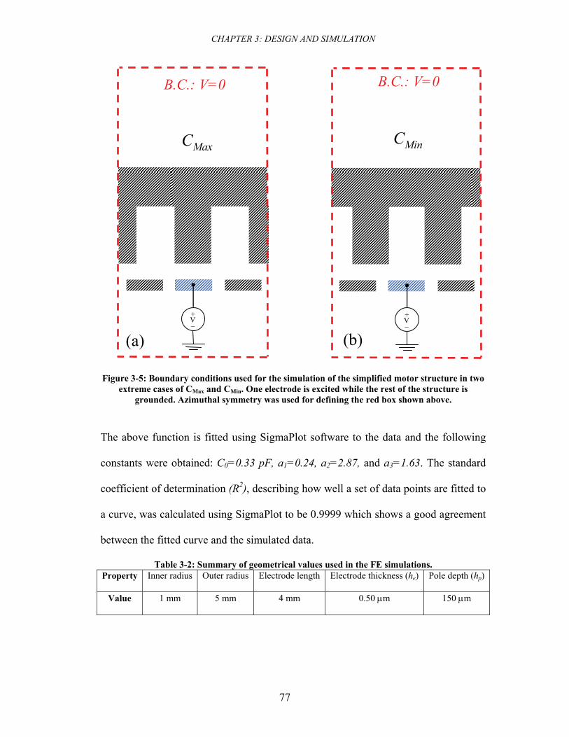
CHAPTER 3: DESIGN AND SIMULATION
77
B.C.: V=0 B.C.: V=0
+_V
+_V
CMinCMax
(a) (b)
Figure 3-5: Boundary conditions used for the simulation of the simplified motor structure in two extreme cases of CMax and CMin. One electrode is excited while the rest of the structure is
grounded. Azimuthal symmetry was used for defining the red box shown above. The above function is fitted using SigmaPlot software to the data and the following
constants were obtained: C0=0.33 pF, a1=0.24, a2=2.87, and a3=1.63. The standard
coefficient of determination (R2), describing how well a set of data points are fitted to
a curve, was calculated using SigmaPlot to be 0.9999 which shows a good agreement
between the fitted curve and the simulated data.
Table 3-2: Summary of geometrical values used in the FE simulations. Property Inner radius Outer radius Electrode length Electrode thickness (he) Pole depth (hp)
Value 1 mm 5 mm 4 mm 0.50 μm 150 μm
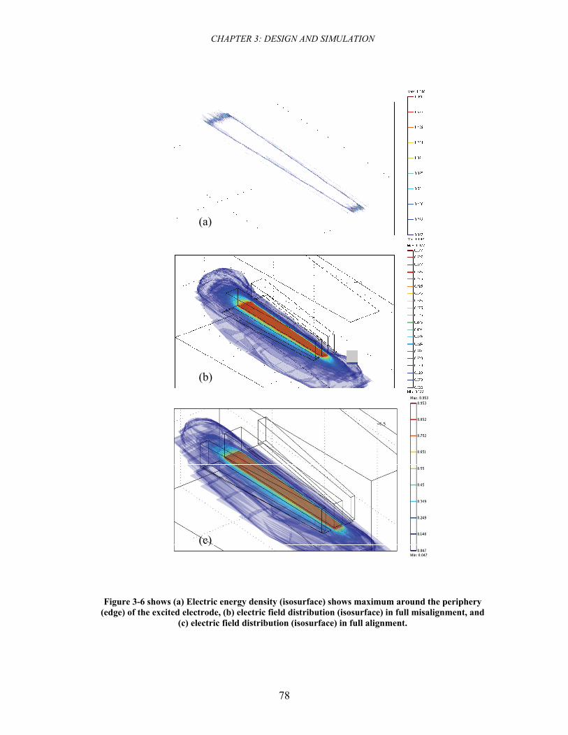
CHAPTER 3: DESIGN AND SIMULATION
78
(a)
(b)
(c)
Figure 3-6 shows (a) Electric energy density (isosurface) shows maximum around the periphery (edge) of the excited electrode, (b) electric field distribution (isosurface) in full misalignment, and
(c) electric field distribution (isosurface) in full alignment.
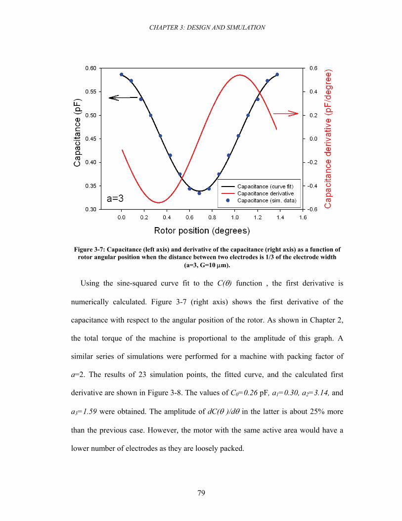
CHAPTER 3: DESIGN AND SIMULATION
79
Figure 3-7: Capacitance (left axis) and derivative of the capacitance (right axis) as a function of rotor angular position when the distance between two electrodes is 1/3 of the electrode width
(a=3, G=10 μm).
Using the sine-squared curve fit to the C(θ) function , the first derivative is
numerically calculated. Figure 3-7 (right axis) shows the first derivative of the
capacitance with respect to the angular position of the rotor. As shown in Chapter 2,
the total torque of the machine is proportional to the amplitude of this graph. A
similar series of simulations were performed for a machine with packing factor of
a=2. The results of 23 simulation points, the fitted curve, and the calculated first
derivative are shown in Figure 3-8. The values of C0=0.26 pF, a1=0.30, a2=3.14, and
a3=1.59 were obtained. The amplitude of dC(θ )/dθ in the latter is about 25% more
than the previous case. However, the motor with the same active area would have a
lower number of electrodes as they are loosely packed.
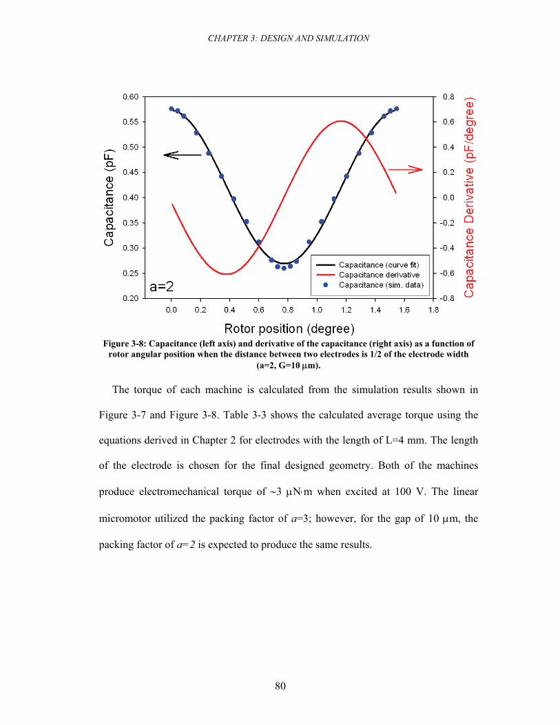
CHAPTER 3: DESIGN AND SIMULATION
80
Figure 3-8: Capacitance (left axis) and derivative of the capacitance (right axis) as a function of
rotor angular position when the distance between two electrodes is 1/2 of the electrode width (a=2, G=10 μm).
The torque of each machine is calculated from the simulation results shown in
Figure 3-7 and Figure 3-8. Table 3-3 shows the calculated average torque using the
equations derived in Chapter 2 for electrodes with the length of L=4 mm. The length
of the electrode is chosen for the final designed geometry. Both of the machines
produce electromechanical torque of ∼3 μN⋅m when excited at 100 V. The linear
micromotor utilized the packing factor of a=3; however, for the gap of 10 μm, the
packing factor of a=2 is expected to produce the same results.
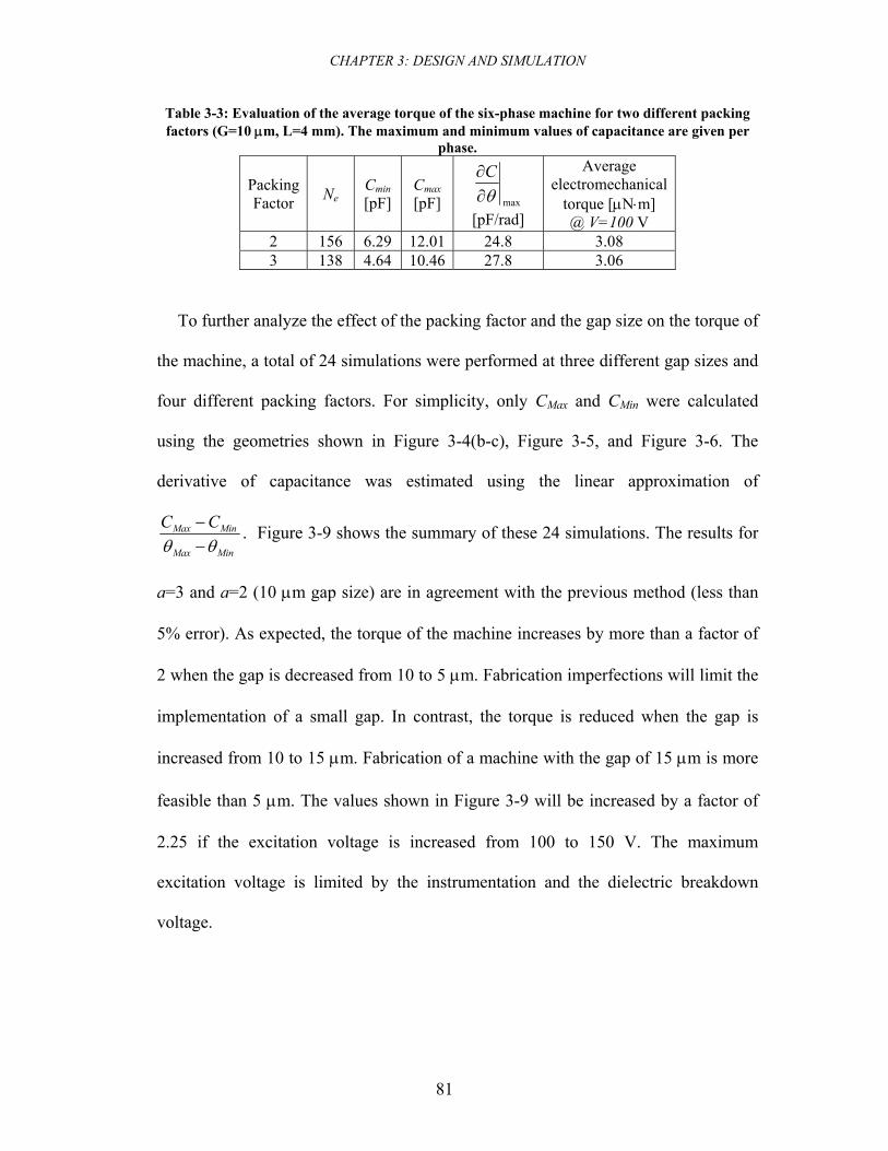
CHAPTER 3: DESIGN AND SIMULATION
81
Table 3-3: Evaluation of the average torque of the six-phase machine for two different packing factors (G=10 μm, L=4 mm). The maximum and minimum values of capacitance are given per
phase.
Packing Factor Ne
Cmin [pF]
Cmax [pF] maxθ∂
∂C
[pF/rad]
Average electromechanical
torque [μN⋅m] @ V=100 V
2 156 6.29 12.01 24.8 3.08 3 138 4.64 10.46 27.8 3.06
To further analyze the effect of the packing factor and the gap size on the torque of
the machine, a total of 24 simulations were performed at three different gap sizes and
four different packing factors. For simplicity, only CMax and CMin were calculated
using the geometries shown in Figure 3-4(b-c), Figure 3-5, and Figure 3-6. The
derivative of capacitance was estimated using the linear approximation of
MinMax
MinMax CCθθ −
− . Figure 3-9 shows the summary of these 24 simulations. The results for
a=3 and a=2 (10 μm gap size) are in agreement with the previous method (less than
5% error). As expected, the torque of the machine increases by more than a factor of
2 when the gap is decreased from 10 to 5 μm. Fabrication imperfections will limit the
implementation of a small gap. In contrast, the torque is reduced when the gap is
increased from 10 to 15 μm. Fabrication of a machine with the gap of 15 μm is more
feasible than 5 μm. The values shown in Figure 3-9 will be increased by a factor of
2.25 if the excitation voltage is increased from 100 to 150 V. The maximum
excitation voltage is limited by the instrumentation and the dielectric breakdown
voltage.
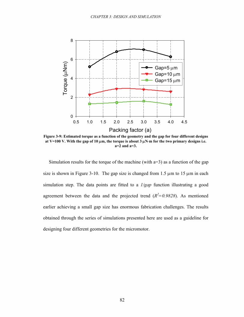
CHAPTER 3: DESIGN AND SIMULATION
82
Packing factor (a)0.5 1.0 1.5 2.0 2.5 3.0 3.5 4.0 4.5
Torq
ue (μ
Nm
)
0
2
4
6
8
Gap=5 μmGap=10 μmGap=15 μm
Figure 3-9: Estimated torque as a function of the geometry and the gap for four different designs at V=100 V. With the gap of 10 μm, the torque is about 3 μN⋅m for the two primary designs i.e.
a=2 and a=3.
Simulation results for the torque of the machine (with a=3) as a function of the gap
size is shown in Figure 3-10. The gap size is changed from 1.5 μm to 15 μm in each
simulation step. The data points are fitted to a 1/gap function illustrating a good
agreement between the data and the projected trend (R2=0.9828). As mentioned
earlier achieving a small gap size has enormous fabrication challenges. The results
obtained through the series of simulations presented here are used as a guideline for
designing four different geometries for the micromotor.
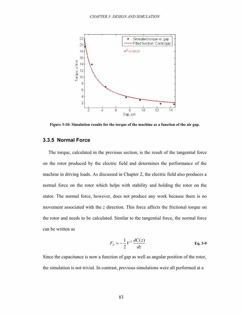
CHAPTER 3: DESIGN AND SIMULATION
83
Figure 3-10: Simulation results for the torque of the machine as a function of the air gap.
3.3.5 Normal Force
The torque, calculated in the previous section, is the result of the tangential force
on the rotor produced by the electric field and determines the performance of the
machine in driving loads. As discussed in Chapter 2, the electric field also produces a
normal force on the rotor which helps with stability and holding the rotor on the
stator. The normal force, however, does not produce any work because there is no
movement associated with the z direction. This force affects the frictional torque on
the rotor and needs to be calculated. Similar to the tangential force, the normal force
can be written as
dzzdCVFZ)(
21 2−= Eq. 3-9
Since the capacitance is now a function of gap as well as angular position of the rotor,
the simulation is not trivial. In contrast, previous simulations were all performed at a
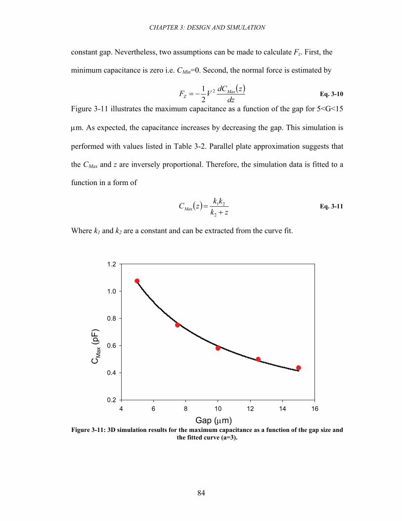
CHAPTER 3: DESIGN AND SIMULATION
84
constant gap. Nevertheless, two assumptions can be made to calculate Fz. First, the
minimum capacitance is zero i.e. CMin=0. Second, the normal force is estimated by
( )dz
zdCVF MaxZ
2
21
−= Eq. 3-10
Figure 3-11 illustrates the maximum capacitance as a function of the gap for 5<G<15
μm. As expected, the capacitance increases by decreasing the gap. This simulation is
performed with values listed in Table 3-2. Parallel plate approximation suggests that
the CMax and z are inversely proportional. Therefore, the simulation data is fitted to a
function in a form of
( )zk
kkzCMax +=
2
21 Eq. 3-11
Where k1 and k2 are a constant and can be extracted from the curve fit.
4 6 8 10 12 14 160.2
0.4
0.6
0.8
1.0
1.2
Gap (μm)
CM
ax (p
F)
Figure 3-11: 3D simulation results for the maximum capacitance as a function of the gap size and
the fitted curve (a=3).
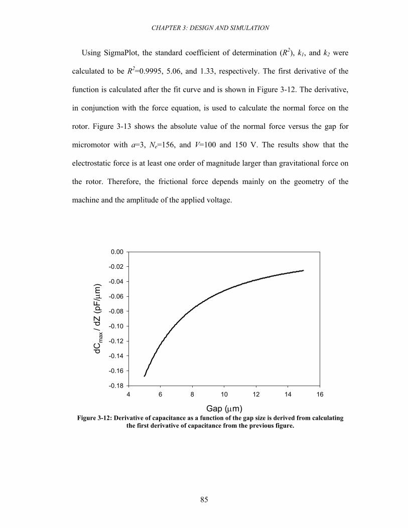
CHAPTER 3: DESIGN AND SIMULATION
85
Using SigmaPlot, the standard coefficient of determination (R2), k1, and k2 were
calculated to be R2=0.9995, 5.06, and 1.33, respectively. The first derivative of the
function is calculated after the fit curve and is shown in Figure 3-12. The derivative,
in conjunction with the force equation, is used to calculate the normal force on the
rotor. Figure 3-13 shows the absolute value of the normal force versus the gap for
micromotor with a=3, Ne=156, and V=100 and 150 V. The results show that the
electrostatic force is at least one order of magnitude larger than gravitational force on
the rotor. Therefore, the frictional force depends mainly on the geometry of the
machine and the amplitude of the applied voltage.
Gap (μm)
4 6 8 10 12 14 16
dCm
ax /
dZ (p
F/μ m
)
-0.18
-0.16
-0.14
-0.12
-0.10
-0.08
-0.06
-0.04
-0.02
0.00
Figure 3-12: Derivative of capacitance as a function of the gap size is derived from calculating
the first derivative of capacitance from the previous figure.
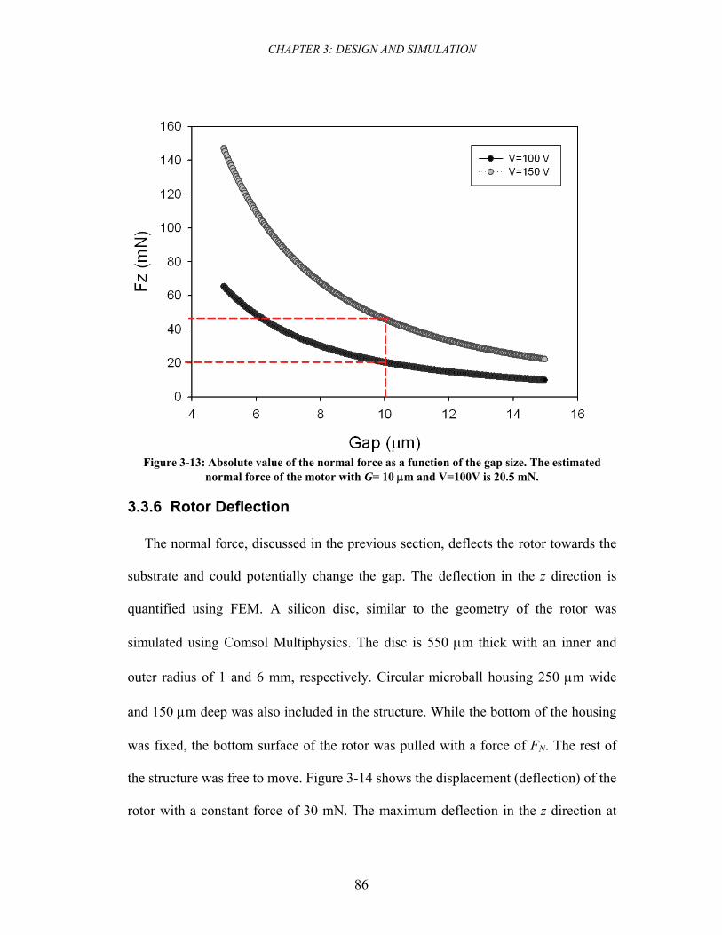
CHAPTER 3: DESIGN AND SIMULATION
86
Figure 3-13: Absolute value of the normal force as a function of the gap size. The estimated
normal force of the motor with G= 10 μm and V=100V is 20.5 mN.
3.3.6 Rotor Deflection
The normal force, discussed in the previous section, deflects the rotor towards the
substrate and could potentially change the gap. The deflection in the z direction is
quantified using FEM. A silicon disc, similar to the geometry of the rotor was
simulated using Comsol Multiphysics. The disc is 550 μm thick with an inner and
outer radius of 1 and 6 mm, respectively. Circular microball housing 250 μm wide
and 150 μm deep was also included in the structure. While the bottom of the housing
was fixed, the bottom surface of the rotor was pulled with a force of FN. The rest of
the structure was free to move. Figure 3-14 shows the displacement (deflection) of the
rotor with a constant force of 30 mN. The maximum deflection in the z direction at
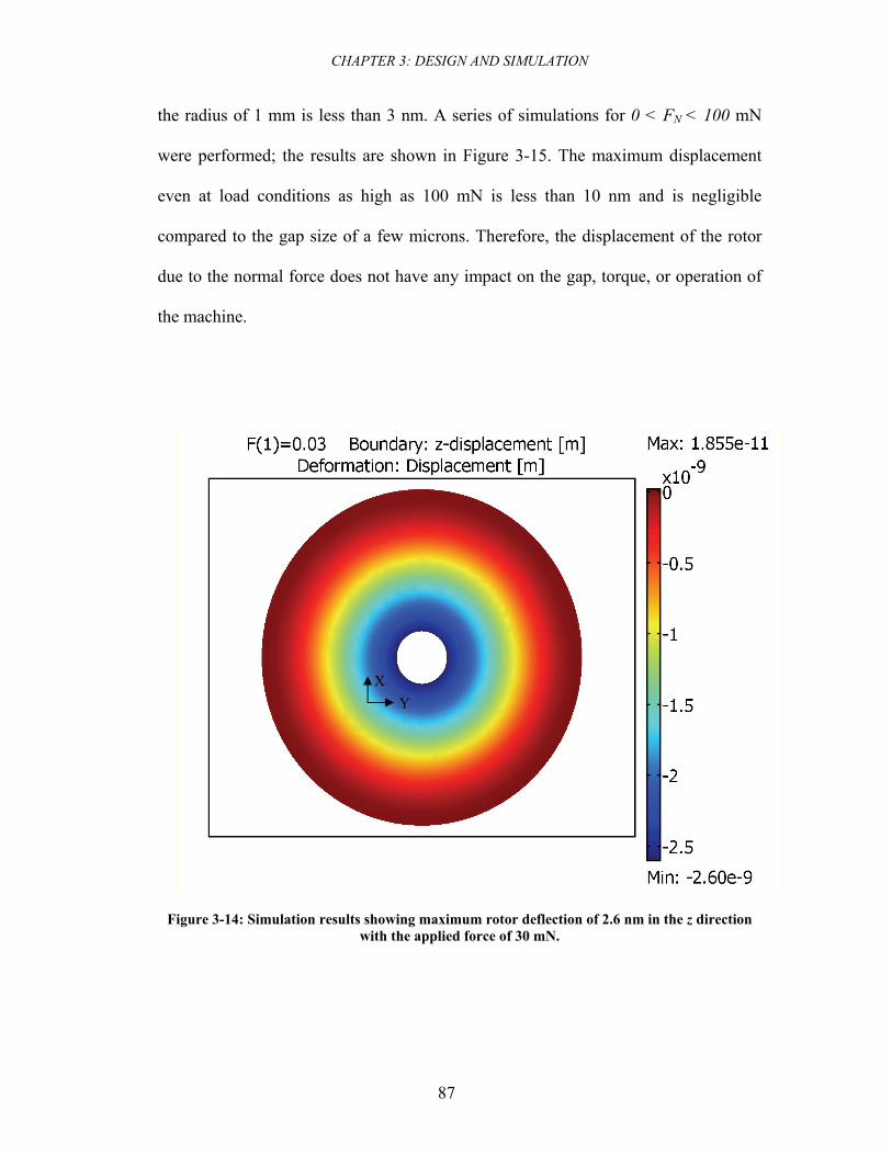
CHAPTER 3: DESIGN AND SIMULATION
87
the radius of 1 mm is less than 3 nm. A series of simulations for 0 < FN < 100 mN
were performed; the results are shown in Figure 3-15. The maximum displacement
even at load conditions as high as 100 mN is less than 10 nm and is negligible
compared to the gap size of a few microns. Therefore, the displacement of the rotor
due to the normal force does not have any impact on the gap, torque, or operation of
the machine.
Figure 3-14: Simulation results showing maximum rotor deflection of 2.6 nm in the z direction with the applied force of 30 mN.
XY
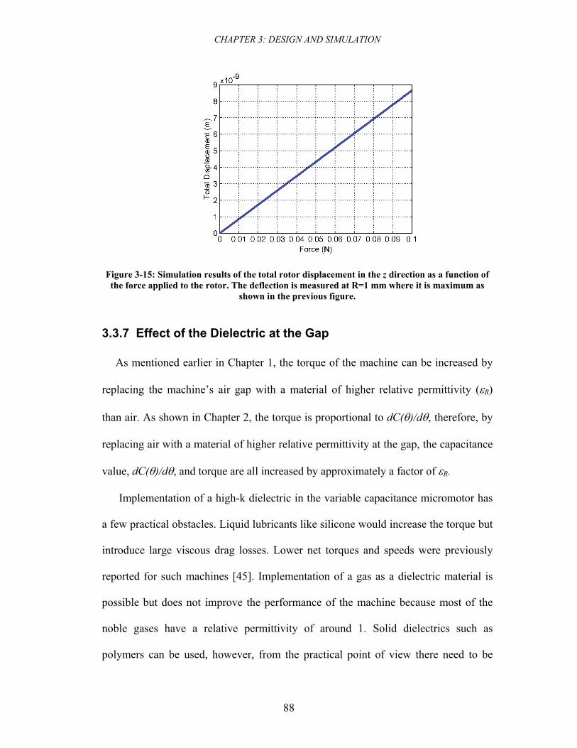
CHAPTER 3: DESIGN AND SIMULATION
88
Figure 3-15: Simulation results of the total rotor displacement in the z direction as a function of the force applied to the rotor. The deflection is measured at R=1 mm where it is maximum as
shown in the previous figure.
3.3.7 Effect of the Dielectric at the Gap
As mentioned earlier in Chapter 1, the torque of the machine can be increased by
replacing the machine’s air gap with a material of higher relative permittivity (εR)
than air. As shown in Chapter 2, the torque is proportional to dC(θ)/dθ, therefore, by
replacing air with a material of higher relative permittivity at the gap, the capacitance
value, dC(θ)/dθ, and torque are all increased by approximately a factor of εR.
Implementation of a high-k dielectric in the variable capacitance micromotor has
a few practical obstacles. Liquid lubricants like silicone would increase the torque but
introduce large viscous drag losses. Lower net torques and speeds were previously
reported for such machines [45]. Implementation of a gas as a dielectric material is
possible but does not improve the performance of the machine because most of the
noble gases have a relative permittivity of around 1. Solid dielectrics such as
polymers can be used, however, from the practical point of view there need to be
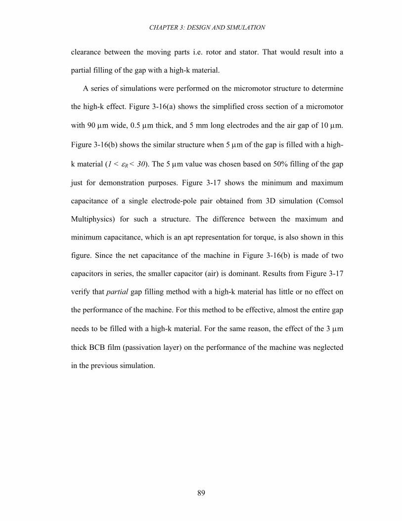
CHAPTER 3: DESIGN AND SIMULATION
89
clearance between the moving parts i.e. rotor and stator. That would result into a
partial filling of the gap with a high-k material.
A series of simulations were performed on the micromotor structure to determine
the high-k effect. Figure 3-16(a) shows the simplified cross section of a micromotor
with 90 μm wide, 0.5 μm thick, and 5 mm long electrodes and the air gap of 10 μm.
Figure 3-16(b) shows the similar structure when 5 μm of the gap is filled with a high-
k material (1 < εR < 30). The 5 μm value was chosen based on 50% filling of the gap
just for demonstration purposes. Figure 3-17 shows the minimum and maximum
capacitance of a single electrode-pole pair obtained from 3D simulation (Comsol
Multiphysics) for such a structure. The difference between the maximum and
minimum capacitance, which is an apt representation for torque, is also shown in this
figure. Since the net capacitance of the machine in Figure 3-16(b) is made of two
capacitors in series, the smaller capacitor (air) is dominant. Results from Figure 3-17
verify that partial gap filling method with a high-k material has little or no effect on
the performance of the machine. For this method to be effective, almost the entire gap
needs to be filled with a high-k material. For the same reason, the effect of the 3 μm
thick BCB film (passivation layer) on the performance of the machine was neglected
in the previous simulation.
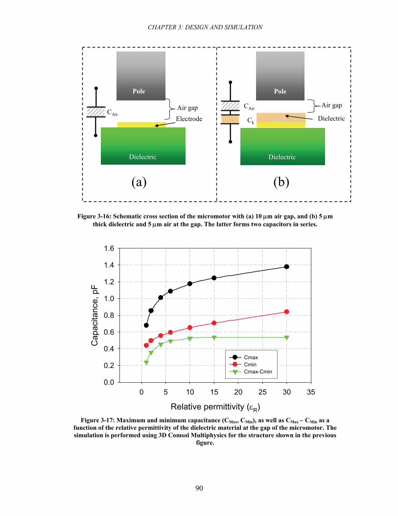
CHAPTER 3: DESIGN AND SIMULATION
90
Air gap
Dielectric
Dielectric
Air gapElectrode
Dielectric
PolePole
CAir
Ck
(a) (b)
CAir
Figure 3-16: Schematic cross section of the micromotor with (a) 10 μm air gap, and (b) 5 μm thick dielectric and 5 μm air at the gap. The latter forms two capacitors in series.
Relative permittivity (εR)
0 5 10 15 20 25 30 35
Cap
acita
nce,
pF
0.0
0.2
0.4
0.6
0.8
1.0
1.2
1.4
1.6
CmaxCmin Cmax-Cmin
Figure 3-17: Maximum and minimum capacitance (CMax, CMin), as well as CMax − CMin as a
function of the relative permittivity of the dielectric material at the gap of the micromotor. The simulation is performed using 3D Comsol Multiphysics for the structure shown in the previous
figure.
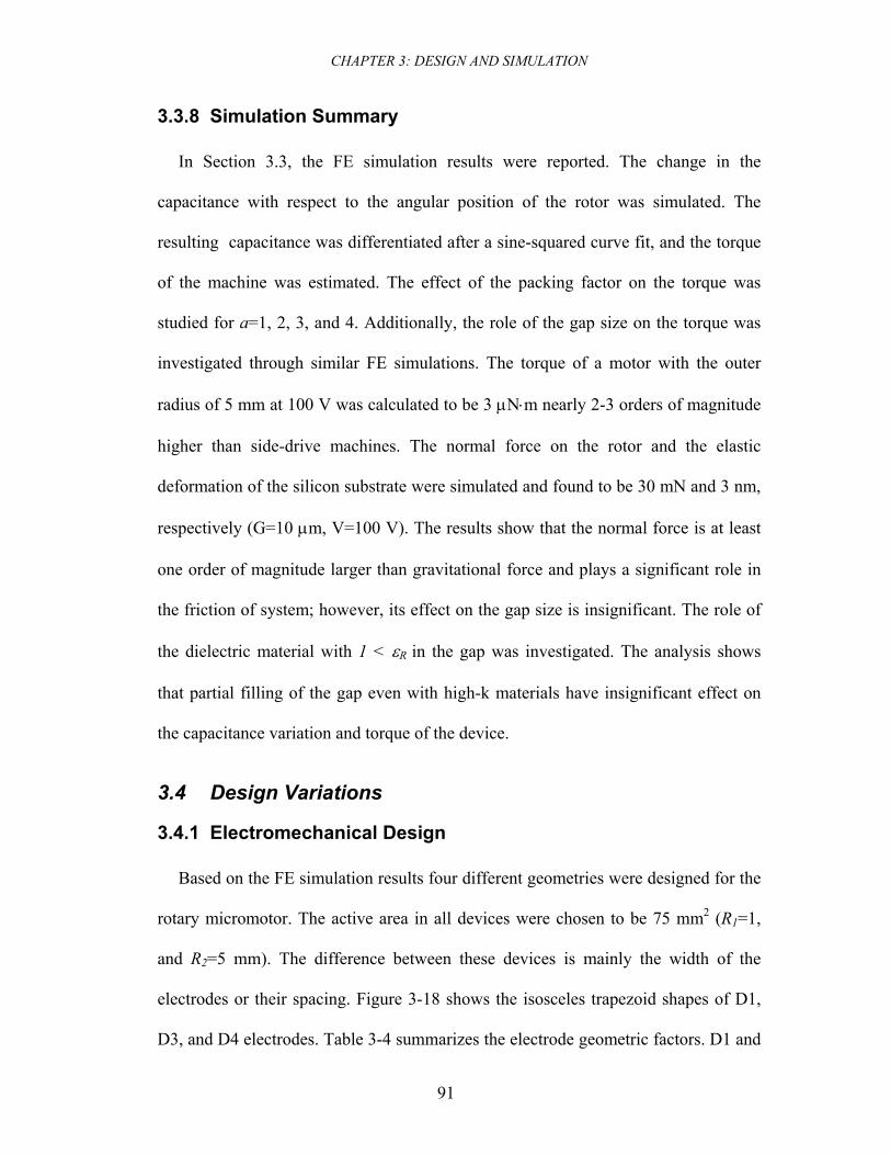
CHAPTER 3: DESIGN AND SIMULATION
91
3.3.8 Simulation Summary
In Section 3.3, the FE simulation results were reported. The change in the
capacitance with respect to the angular position of the rotor was simulated. The
resulting capacitance was differentiated after a sine-squared curve fit, and the torque
of the machine was estimated. The effect of the packing factor on the torque was
studied for a=1, 2, 3, and 4. Additionally, the role of the gap size on the torque was
investigated through similar FE simulations. The torque of a motor with the outer
radius of 5 mm at 100 V was calculated to be 3 μN⋅m nearly 2-3 orders of magnitude
higher than side-drive machines. The normal force on the rotor and the elastic
deformation of the silicon substrate were simulated and found to be 30 mN and 3 nm,
respectively (G=10 μm, V=100 V). The results show that the normal force is at least
one order of magnitude larger than gravitational force and plays a significant role in
the friction of system; however, its effect on the gap size is insignificant. The role of
the dielectric material with 1 < εR in the gap was investigated. The analysis shows
that partial filling of the gap even with high-k materials have insignificant effect on
the capacitance variation and torque of the device.
3.4 Design Variations
3.4.1 Electromechanical Design
Based on the FE simulation results four different geometries were designed for the
rotary micromotor. The active area in all devices were chosen to be 75 mm2 (R1=1,
and R2=5 mm). The difference between these devices is mainly the width of the
electrodes or their spacing. Figure 3-18 shows the isosceles trapezoid shapes of D1,
D3, and D4 electrodes. Table 3-4 summarizes the electrode geometric factors. D1 and
CHAPTER 3: DESIGN AND SIMULATION
92
D2 are designed based on the gap size of 10 μm. D4 is designed to have electrodes
with half the width of D1 for the gap of 5 μm. Finally, D3 is designed to have a high
synchronous speed i.e. small number of electrodes. Theoretically, the smallest
number of electrode is 6; however, such a machine does not produce significant
torque. Consequently 30 electrodes were chosen for D3.
Figure 3-18: Electrode geometry for design (a) D1, (b) D3, and (c) D4.
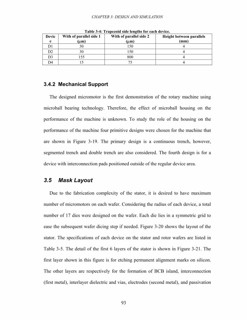
CHAPTER 3: DESIGN AND SIMULATION
93
Table 3-4: Trapezoid side lengths for each device. Devic
e With of parallel side 1
(μm) With of parallel side 2
(μm) Height between parallels
(mm) D1 30 150 4 D2 30 150 4 D3 155 800 4 D4 15 75 4
3.4.2 Mechanical Support
The designed micromotor is the first demonstration of the rotary machine using
microball bearing technology. Therefore, the effect of microball housing on the
performance of the machine is unknown. To study the role of the housing on the
performance of the machine four primitive designs were chosen for the machine that
are shown in Figure 3-19. The primary design is a continuous trench, however,
segmented trench and double trench are also considered. The fourth design is for a
device with interconnection pads positioned outside of the regular device area.
3.5 Mask Layout
Due to the fabrication complexity of the stator, it is desired to have maximum
number of micromotors on each wafer. Considering the radius of each device, a total
number of 17 dies were designed on the wafer. Each die lies in a symmetric grid to
ease the subsequent wafer dicing step if needed. Figure 3-20 shows the layout of the
stator. The specifications of each device on the stator and rotor wafers are listed in
Table 3-5. The detail of the first 6 layers of the stator is shown in Figure 3-21. The
first layer shown in this figure is for etching permanent alignment marks on silicon.
The other layers are respectively for the formation of BCB island, interconnection
(first metal), interlayer dielectric and vias, electrodes (second metal), and passivation
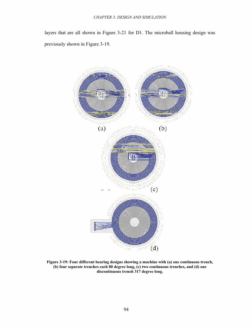
CHAPTER 3: DESIGN AND SIMULATION
94
layers that are all shown in Figure 3-21 for D1. The microball housing design was
previously shown in Figure 3-19.
Figure 3-19: Four different bearing designs showing a machine with (a) one continuous trench, (b) four separate trenches each 80 degree long, (c) two continuous trenches, and (d) one
discontinuous trench 317 degree long.
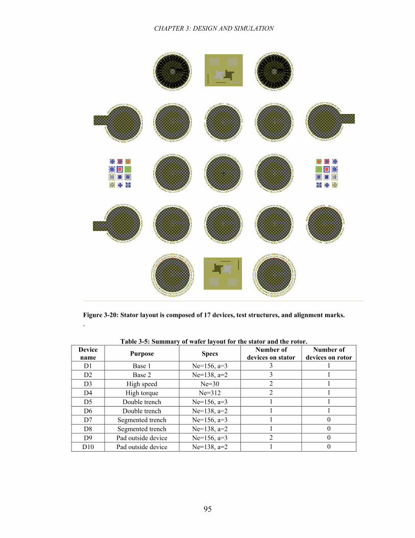
CHAPTER 3: DESIGN AND SIMULATION
95
Figure 3-20: Stator layout is composed of 17 devices, test structures, and alignment marks. .
Table 3-5: Summary of wafer layout for the stator and the rotor. Device name Purpose Specs Number of
devices on stator Number of
devices on rotor D1 Base 1 Ne=156, a=3 3 1 D2 Base 2 Ne=138, a=2 3 1 D3 High speed Ne=30 2 1 D4 High torque Ne=312 2 1 D5 Double trench Ne=156, a=3 1 1 D6 Double trench Ne=138, a=2 1 1 D7 Segmented trench Ne=156, a=3 1 0 D8 Segmented trench Ne=138, a=2 1 0 D9 Pad outside device Ne=156, a=3 2 0 D10 Pad outside device Ne=138, a=2 1 0
CHAPTER 3: DESIGN AND SIMULATION
96
Figure 3-21: First 6 layers on the stator composed of (a) silicon pit, (b) BCB island, (c) interconnection, (d) interlayer dielectric, (e) electrodes, and (f) passivation.
Unlike the stator, the rotor layout is composed of only six devices. This is to
reduce the loading in the DRIE steps which is explained in Chapter 4. Since the
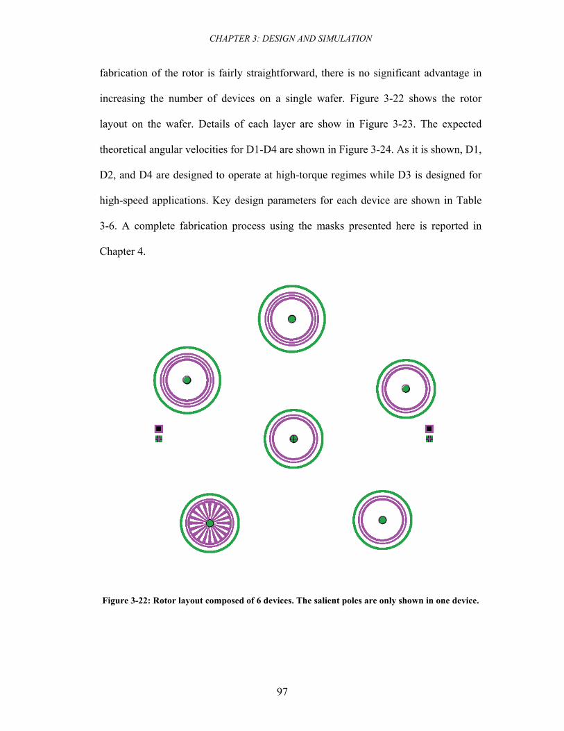
CHAPTER 3: DESIGN AND SIMULATION
97
fabrication of the rotor is fairly straightforward, there is no significant advantage in
increasing the number of devices on a single wafer. Figure 3-22 shows the rotor
layout on the wafer. Details of each layer are show in Figure 3-23. The expected
theoretical angular velocities for D1-D4 are shown in Figure 3-24. As it is shown, D1,
D2, and D4 are designed to operate at high-torque regimes while D3 is designed for
high-speed applications. Key design parameters for each device are shown in Table
3-6. A complete fabrication process using the masks presented here is reported in
Chapter 4.
Figure 3-22: Rotor layout composed of 6 devices. The salient poles are only shown in one device.
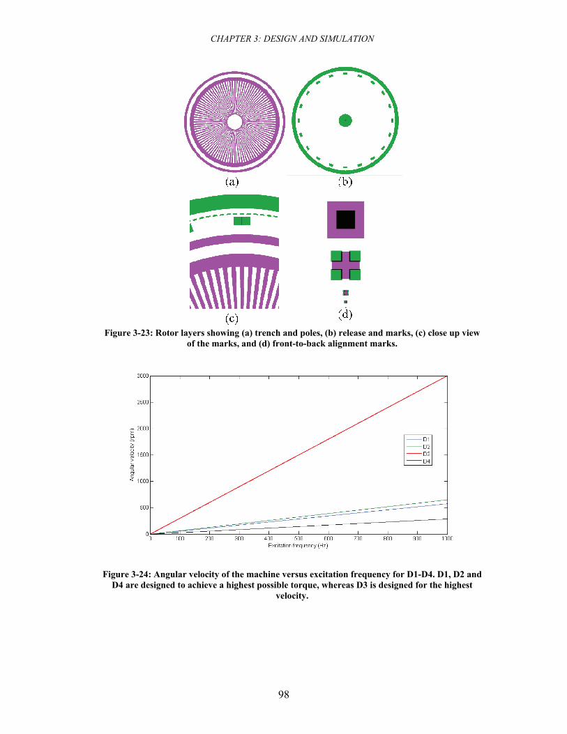
CHAPTER 3: DESIGN AND SIMULATION
98
Figure 3-23: Rotor layers showing (a) trench and poles, (b) release and marks, (c) close up view
of the marks, and (d) front-to-back alignment marks.
Figure 3-24: Angular velocity of the machine versus excitation frequency for D1-D4. D1, D2 and D4 are designed to achieve a highest possible torque, whereas D3 is designed for the highest
velocity.
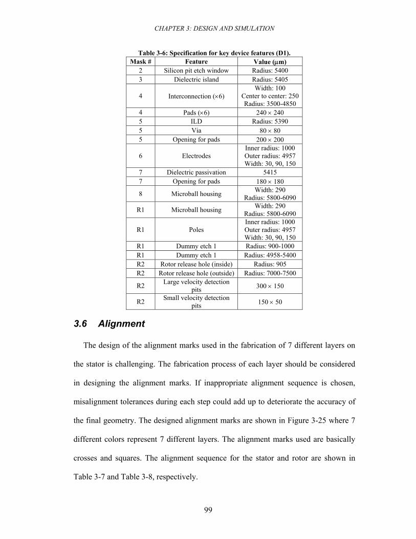
CHAPTER 3: DESIGN AND SIMULATION
99
Table 3-6: Specification for key device features (D1). Mask # Feature Value (μm)
2 Silicon pit etch window Radius: 5400 3 Dielectric island Radius: 5405
4 Interconnection (×6) Width: 100
Center to center: 250 Radius: 3500-4850
4 Pads (×6) 240 × 240 5 ILD Radius: 5390 5 Via 80 × 80 5 Opening for pads 200 × 200
6 Electrodes Inner radius: 1000 Outer radius: 4957 Width: 30, 90, 150
7 Dielectric passivation 5415 7 Opening for pads 180 × 180
8 Microball housing Width: 290 Radius: 5800-6090
R1 Microball housing Width: 290 Radius: 5800-6090
R1 Poles Inner radius: 1000 Outer radius: 4957 Width: 30, 90, 150
R1 Dummy etch 1 Radius: 900-1000 R1 Dummy etch 1 Radius: 4958-5400 R2 Rotor release hole (inside) Radius: 905 R2 Rotor release hole (outside) Radius: 7000-7500
R2 Large velocity detection pits 300 × 150
R2 Small velocity detection pits 150 × 50
3.6 Alignment
The design of the alignment marks used in the fabrication of 7 different layers on
the stator is challenging. The fabrication process of each layer should be considered
in designing the alignment marks. If inappropriate alignment sequence is chosen,
misalignment tolerances during each step could add up to deteriorate the accuracy of
the final geometry. The designed alignment marks are shown in Figure 3-25 where 7
different colors represent 7 different layers. The alignment marks used are basically
crosses and squares. The alignment sequence for the stator and rotor are shown in
Table 3-7 and Table 3-8, respectively.
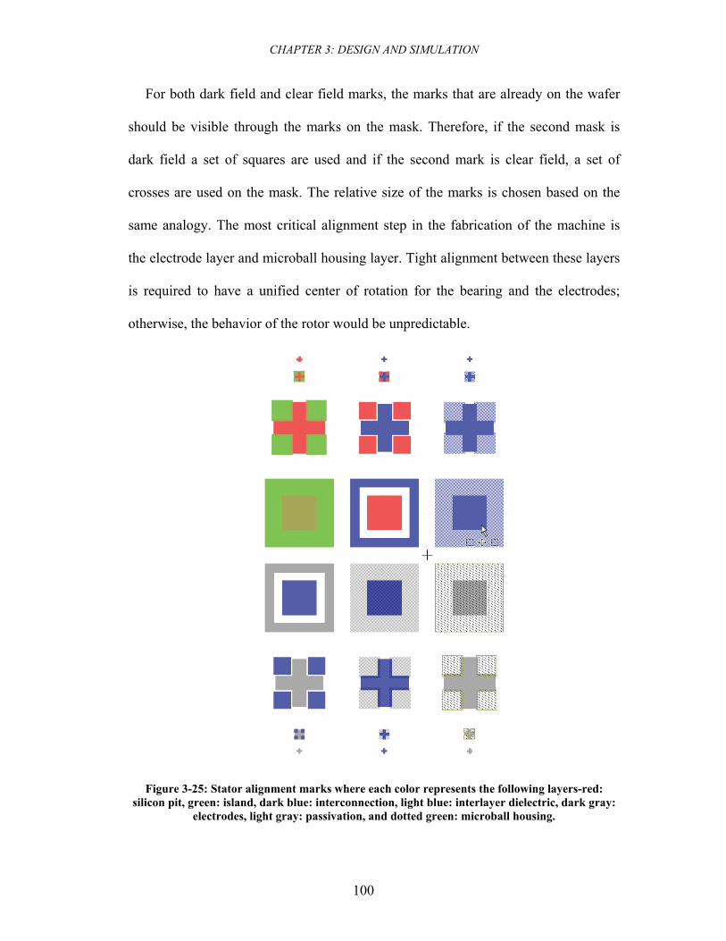
CHAPTER 3: DESIGN AND SIMULATION
100
For both dark field and clear field marks, the marks that are already on the wafer
should be visible through the marks on the mask. Therefore, if the second mask is
dark field a set of squares are used and if the second mark is clear field, a set of
crosses are used on the mask. The relative size of the marks is chosen based on the
same analogy. The most critical alignment step in the fabrication of the machine is
the electrode layer and microball housing layer. Tight alignment between these layers
is required to have a unified center of rotation for the bearing and the electrodes;
otherwise, the behavior of the rotor would be unpredictable.
Figure 3-25: Stator alignment marks where each color represents the following layers-red: silicon pit, green: island, dark blue: interconnection, light blue: interlayer dielectric, dark gray:
electrodes, light gray: passivation, and dotted green: microball housing.
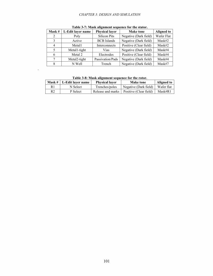
CHAPTER 3: DESIGN AND SIMULATION
101
Table 3-7: Mask alignment sequence for the stator. Mask # L-Edit layer name Physical layer Make tone Aligned to
2 Poly Silicon Pits Negative (Dark field) Wafer Flat 3 Active BCB Islands Negative (Dark field) Mask#2 4 Metal1 Interconnects Positive (Clear field) Mask#2 5 Metal1-tight Vias Negative (Dark field) Mask#4 6 Metal 2 Electrodes Positive (Clear field) Mask#4 7 Metal2-tight Passivation/Pads Negative (Dark field) Mask#4 8 N Well Trench Negative (Dark field) Mask#7
.
Table 3-8: Mask alignment sequence for the rotor. Mask # L-Edit layer name Physical layer Make tone Aligned to
R1 N Select Trenches/poles Negative (Dark field) Wafer flat R2 P Select Release and marks Positive (Clear field) Mask#R1
CHAPTER 4: FABRICATION
102
4 Fabrication
4.1 Introduction
One of the major challenges in the development of the micromotor has been the
fabrication of the device. The micromachine, as discussed in chapters 2 and 3, is
made of a micro fabricated stator and rotor. The stator is composed of five layers of
thin films (dielectric or conductor) on the silicon substrate and bulk micromachined
silicon structures for microball housing. The large number of layers, together with the
use of a low-k polymer in the structure of the stator, has made the fabrication process
extremely complex. The stator fabrication process consists of 7 major steps each
composed of a few sub steps. The rotor process is less complicated and has three
major steps. Both processes are detailed in the next section.
4.2 Process Flow Design
Four-inch, <100>, p-type, 1-10 Ω⋅cm, 525 ±25 μm thick, double-polished silicon
substrates were used as starting material for the fabrication of the stator and the rotor.
The choice of substrate properties was discussed in Chapter 3. The wafers were
selected to be double polished to make infrared imaging of the balls possible28. The
schematic cross section of the stator fabrication process is shown in Figure 4-1. The
process consists of surface micromachining (thin film deposition and patterning) and
bulk micromachining (deep etching) steps. To keep all photolithography processes
planar, the bulk micromachining is performed at the last step.
28 Infra red imaging was not pursued at the final characterization step.
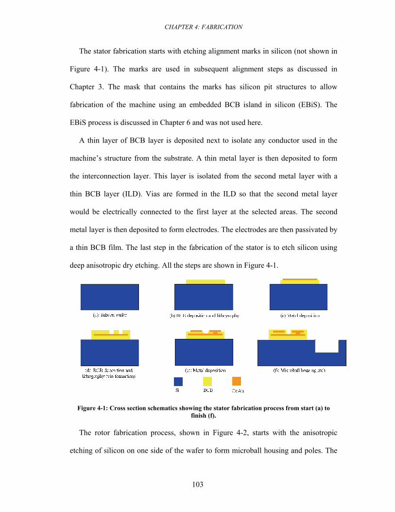
CHAPTER 4: FABRICATION
103
The stator fabrication starts with etching alignment marks in silicon (not shown in
Figure 4-1). The marks are used in subsequent alignment steps as discussed in
Chapter 3. The mask that contains the marks has silicon pit structures to allow
fabrication of the machine using an embedded BCB island in silicon (EBiS). The
EBiS process is discussed in Chapter 6 and was not used here.
A thin layer of BCB layer is deposited next to isolate any conductor used in the
machine’s structure from the substrate. A thin metal layer is then deposited to form
the interconnection layer. This layer is isolated from the second metal layer with a
thin BCB layer (ILD). Vias are formed in the ILD so that the second metal layer
would be electrically connected to the first layer at the selected areas. The second
metal layer is then deposited to form electrodes. The electrodes are then passivated by
a thin BCB film. The last step in the fabrication of the stator is to etch silicon using
deep anisotropic dry etching. All the steps are shown in Figure 4-1.
Figure 4-1: Cross section schematics showing the stator fabrication process from start (a) to finish (f).
The rotor fabrication process, shown in Figure 4-2, starts with the anisotropic
etching of silicon on one side of the wafer to form microball housing and poles. The
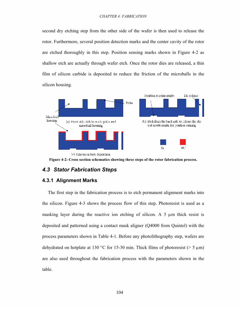
CHAPTER 4: FABRICATION
104
second dry etching step from the other side of the wafer is then used to release the
rotor. Furthermore, several position detection marks and the center cavity of the rotor
are etched thoroughly in this step. Position sensing marks shown in Figure 4-2 as
shallow etch are actually through wafer etch. Once the rotor dies are released, a thin
film of silicon carbide is deposited to reduce the friction of the microballs in the
silicon housing.
Figure 4-2: Cross section schematics showing three steps of the rotor fabrication process.
4.3 Stator Fabrication Steps
4.3.1 Alignment Marks
The first step in the fabrication process is to etch permanent alignment marks into
the silicon. Figure 4-3 shows the process flow of this step. Photoresist is used as a
masking layer during the reactive ion etching of silicon. A 5 μm thick resist is
deposited and patterned using a contact mask aligner (Q4000 from Quintel) with the
process parameters shown in Table 4-1. Before any photolithography step, wafers are
dehydrated on hotplate at 130 °C for 15-30 min. Thick films of photoresist (> 5 μm)
are also used throughout the fabrication process with the parameters shown in the
table.
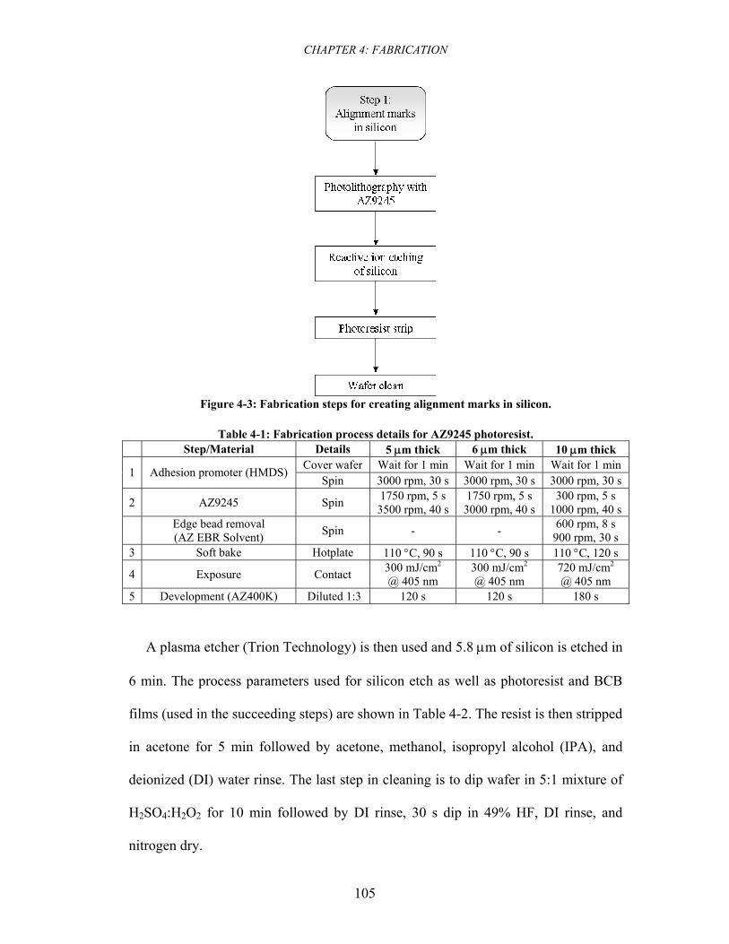
CHAPTER 4: FABRICATION
105
Figure 4-3: Fabrication steps for creating alignment marks in silicon.
Table 4-1: Fabrication process details for AZ9245 photoresist.
Step/Material Details 5 μm thick 6 μm thick 10 μm thick Cover wafer Wait for 1 min Wait for 1 min Wait for 1 min 1 Adhesion promoter (HMDS)
Spin 3000 rpm, 30 s 3000 rpm, 30 s 3000 rpm, 30 s
2 AZ9245 Spin 1750 rpm, 5 s 3500 rpm, 40 s
1750 rpm, 5 s 3000 rpm, 40 s
300 rpm, 5 s 1000 rpm, 40 s
Edge bead removal (AZ EBR Solvent) Spin - - 600 rpm, 8 s
900 rpm, 30 s 3 Soft bake Hotplate 110 °C, 90 s 110 °C, 90 s 110 °C, 120 s
4 Exposure Contact 300 mJ/cm2 @ 405 nm
300 mJ/cm2 @ 405 nm
720 mJ/cm2
@ 405 nm 5 Development (AZ400K) Diluted 1:3 120 s 120 s 180 s
A plasma etcher (Trion Technology) is then used and 5.8 μm of silicon is etched in
6 min. The process parameters used for silicon etch as well as photoresist and BCB
films (used in the succeeding steps) are shown in Table 4-2. The resist is then stripped
in acetone for 5 min followed by acetone, methanol, isopropyl alcohol (IPA), and
deionized (DI) water rinse. The last step in cleaning is to dip wafer in 5:1 mixture of
H2SO4:H2O2 for 10 min followed by DI rinse, 30 s dip in 49% HF, DI rinse, and
nitrogen dry.
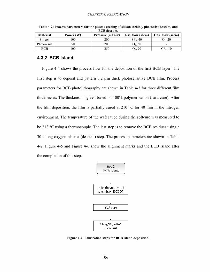
CHAPTER 4: FABRICATION
106
Table 4-2: Process parameters for the plasma etching of silicon etching, photresist descum, and BCB descum.
Material Power (W) Pressure (mTorr) Gas, flow (sccm) Gas, flow (sccm) Silicon 100 200 SF6, 40 O2, 20
Photoresist 50 200 O2, 50 - BCB 100 250 O2, 90 CF4, 10
4.3.2 BCB Island
Figure 4-4 shows the process flow for the deposition of the first BCB layer. The
first step is to deposit and pattern 3.2 μm thick photosensitive BCB film. Process
parameters for BCB photolithography are shown in Table 4-3 for three different film
thicknesses. The thickness is given based on 100% polymerization (hard cure). After
the film deposition, the film is partially cured at 210 °C for 40 min in the nitrogen
environment. The temperature of the wafer tube during the softcure was measured to
be 212 °C using a thermocouple. The last step is to remove the BCB residues using a
30 s long oxygen plasma (descum) step. The process parameters are shown in Table
4-2. Figure 4-5 and Figure 4-6 show the alignment marks and the BCB island after
the completion of this step.
Figure 4-4: Fabrication steps for BCB island deposition.
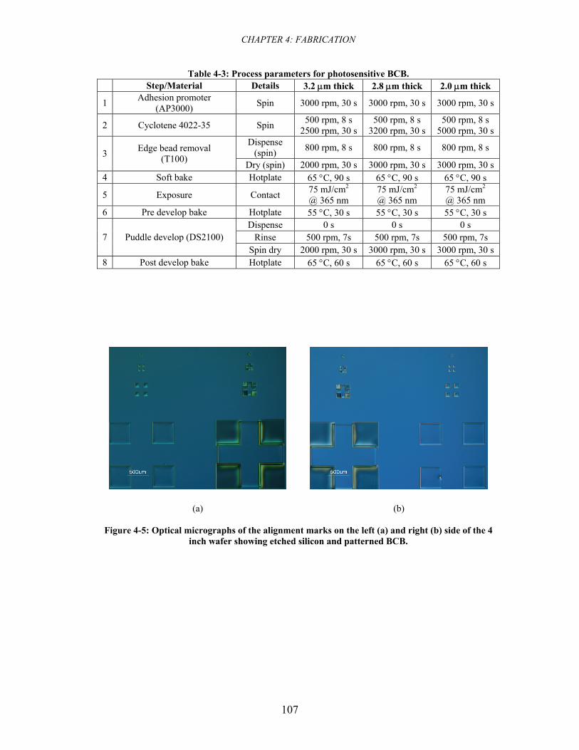
CHAPTER 4: FABRICATION
107
Table 4-3: Process parameters for photosensitive BCB. Step/Material Details 3.2 μm thick 2.8 μm thick 2.0 μm thick
1 Adhesion promoter (AP3000) Spin 3000 rpm, 30 s 3000 rpm, 30 s 3000 rpm, 30 s
2 Cyclotene 4022-35 Spin 500 rpm, 8 s 2500 rpm, 30 s
500 rpm, 8 s 3200 rpm, 30 s
500 rpm, 8 s 5000 rpm, 30 s
Dispense (spin) 800 rpm, 8 s 800 rpm, 8 s 800 rpm, 8 s 3 Edge bead removal
(T100) Dry (spin) 2000 rpm, 30 s 3000 rpm, 30 s 3000 rpm, 30 s 4 Soft bake Hotplate 65 °C, 90 s 65 °C, 90 s 65 °C, 90 s
5 Exposure Contact 75 mJ/cm2 @ 365 nm
75 mJ/cm2 @ 365 nm
75 mJ/cm2 @ 365 nm
6 Pre develop bake Hotplate 55 °C, 30 s 55 °C, 30 s 55 °C, 30 s Dispense 0 s 0 s 0 s
Rinse 500 rpm, 7s 500 rpm, 7s 500 rpm, 7s 7 Puddle develop (DS2100) Spin dry 2000 rpm, 30 s 3000 rpm, 30 s 3000 rpm, 30 s
8 Post develop bake Hotplate 65 °C, 60 s 65 °C, 60 s 65 °C, 60 s
(a)
(b)
Figure 4-5: Optical micrographs of the alignment marks on the left (a) and right (b) side of the 4 inch wafer showing etched silicon and patterned BCB.
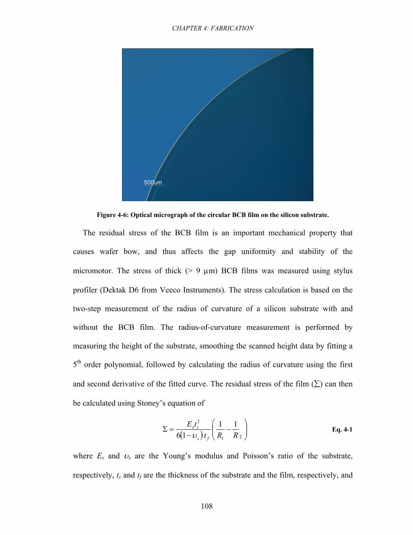
CHAPTER 4: FABRICATION
108
Figure 4-6: Optical micrograph of the circular BCB film on the silicon substrate.
The residual stress of the BCB film is an important mechanical property that
causes wafer bow, and thus affects the gap uniformity and stability of the
micromotor. The stress of thick (> 9 μm) BCB films was measured using stylus
profiler (Dektak D6 from Veeco Instruments). The stress calculation is based on the
two-step measurement of the radius of curvature of a silicon substrate with and
without the BCB film. The radius-of-curvature measurement is performed by
measuring the height of the substrate, smoothing the scanned height data by fitting a
5th order polynomial, followed by calculating the radius of curvature using the first
and second derivative of the fitted curve. The residual stress of the film (∑) can then
be calculated using Stoney’s equation of
( ) ⎟⎟⎠
⎞⎜⎜⎝
⎛−
−=Σ
21
2 1116 RRt
tE
fs
ss
υ Eq. 4-1
where Es and υs are the Young’s modulus and Poisson’s ratio of the substrate,
respectively, ts and tf are the thickness of the substrate and the film, respectively, and
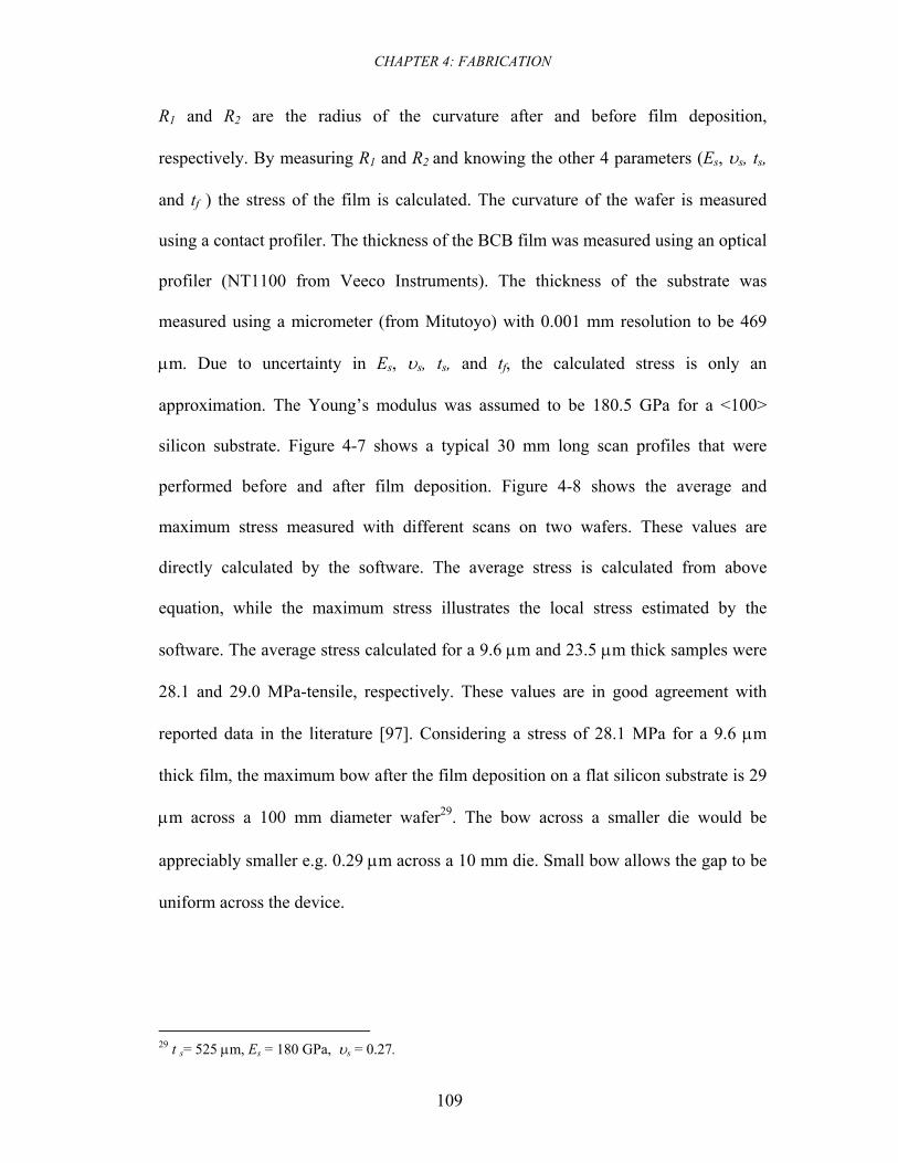
CHAPTER 4: FABRICATION
109
R1 and R2 are the radius of the curvature after and before film deposition,
respectively. By measuring R1 and R2 and knowing the other 4 parameters (Es, υs, ts,
and tf ) the stress of the film is calculated. The curvature of the wafer is measured
using a contact profiler. The thickness of the BCB film was measured using an optical
profiler (NT1100 from Veeco Instruments). The thickness of the substrate was
measured using a micrometer (from Mitutoyo) with 0.001 mm resolution to be 469
μm. Due to uncertainty in Es, υs, ts, and tf, the calculated stress is only an
approximation. The Young’s modulus was assumed to be 180.5 GPa for a <100>
silicon substrate. Figure 4-7 shows a typical 30 mm long scan profiles that were
performed before and after film deposition. Figure 4-8 shows the average and
maximum stress measured with different scans on two wafers. These values are
directly calculated by the software. The average stress is calculated from above
equation, while the maximum stress illustrates the local stress estimated by the
software. The average stress calculated for a 9.6 μm and 23.5 μm thick samples were
28.1 and 29.0 MPa-tensile, respectively. These values are in good agreement with
reported data in the literature [97]. Considering a stress of 28.1 MPa for a 9.6 μm
thick film, the maximum bow after the film deposition on a flat silicon substrate is 29
μm across a 100 mm diameter wafer29. The bow across a smaller die would be
appreciably smaller e.g. 0.29 μm across a 10 mm die. Small bow allows the gap to be
uniform across the device.
29 t s= 525 μm, Es = 180 GPa, υs = 0.27.
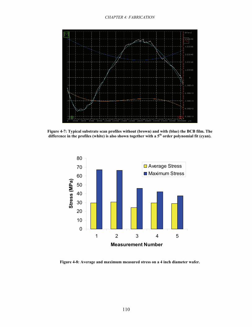
CHAPTER 4: FABRICATION
110
Figure 4-7: Typical substrate scan profiles without (brown) and with (blue) the BCB film. The difference in the profiles (white) is also shown together with a 5th order polynomial fit (cyan).
0
10
20
30
40
50
60
70
80
1 2 3 4 5
Measurement Number
Stre
ss (M
Pa)
Average StressMaximum Stress
Figure 4-8: Average and maximum measured stress on a 4 inch diameter wafer.
CHAPTER 4: FABRICATION
111
4.3.3 Interconnections
The first layer of metal forms an interconnection layer that connects electrodes in
groups of six. The fabrication process is shown in Figure 4-9. After wafer
dehydration, a 20 nm thick chromium film and 250 nm thick gold film are deposited
using a DC magnetron sputtering (AJA International). Process parameters are shown
in Table 4-4. Low deposition power (50 W) is chosen to reduce the penetration of the
metal ions into the polymer. The chromium and gold depositions are performed for 8
and 20 min, respectively. To reduce the contamination effects, the sputtering targets
are conditioned for a few minutes before each deposition.
The metal layers are then patterned with a 5 μm thick photoresist (AZ9245). The
process parameters are summarized in Table 4-1; however, no adhesion promoter
(HMDS) is used here. This ensures a good electrical connection between the
interconnection and electrode layers. Figure 4-10 shows the lithography results. The
gold and chromium layers are then etched using commercial wet etchants (Transene
Company Inc). The gold film is etched for 90 s using TFA etchant at room
temperature, and the chromium is etched for 40 s using TFD etchant at 40 °C.
After inspection, the photoresist is removed using CLK888 photoresist/residue
remover (JT Baker). This step is performed at 60 °C for 5 min. CLK888 is chosen
over other stripers for two reasons. First, the solution is compatible with a number of
low-k dielectrics such as BCB. Second, the solution acts both as a bulk resist striper
and as a residue remover. The latter is important because low ohmic resistance is
required between the two metal layers. Wafers are rinsed with DI, blow dried, and
dehydrated next. The fabrication results are shown in Figure 4-11.
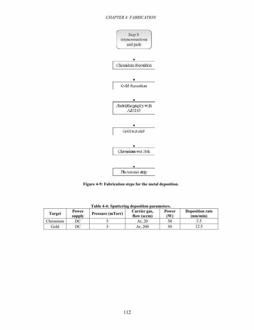
CHAPTER 4: FABRICATION
112
Figure 4-9: Fabrication steps for the metal deposition.
Table 4-4: Sputtering deposition parameters.
Target Power supply Pressure (mTorr) Carrier gas,
flow (sccm) Power
(W) Deposition rate
(nm/min) Chromium DC 5 Ar, 20 50 2.5
Gold DC 5 Ar, 200 50 12.5
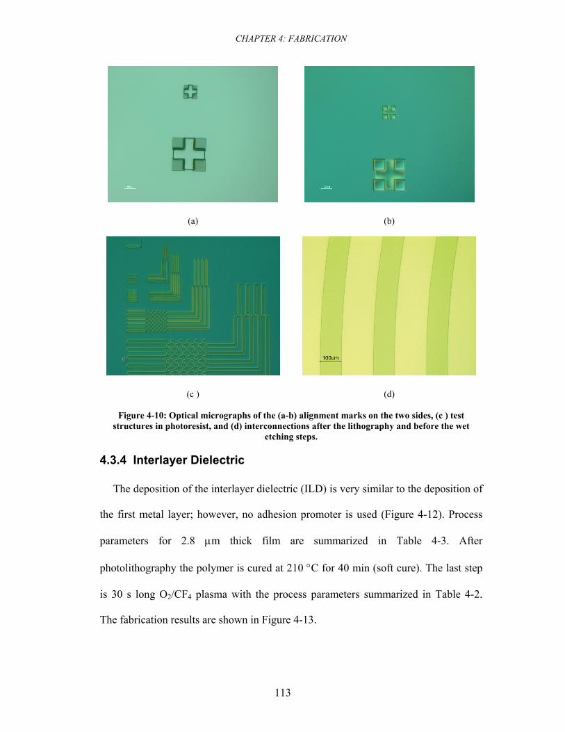
CHAPTER 4: FABRICATION
113
(a)
(b)
(c )
(d)
Figure 4-10: Optical micrographs of the (a-b) alignment marks on the two sides, (c ) test structures in photoresist, and (d) interconnections after the lithography and before the wet
etching steps.
4.3.4 Interlayer Dielectric
The deposition of the interlayer dielectric (ILD) is very similar to the deposition of
the first metal layer; however, no adhesion promoter is used (Figure 4-12). Process
parameters for 2.8 μm thick film are summarized in Table 4-3. After
photolithography the polymer is cured at 210 °C for 40 min (soft cure). The last step
is 30 s long O2/CF4 plasma with the process parameters summarized in Table 4-2.
The fabrication results are shown in Figure 4-13.
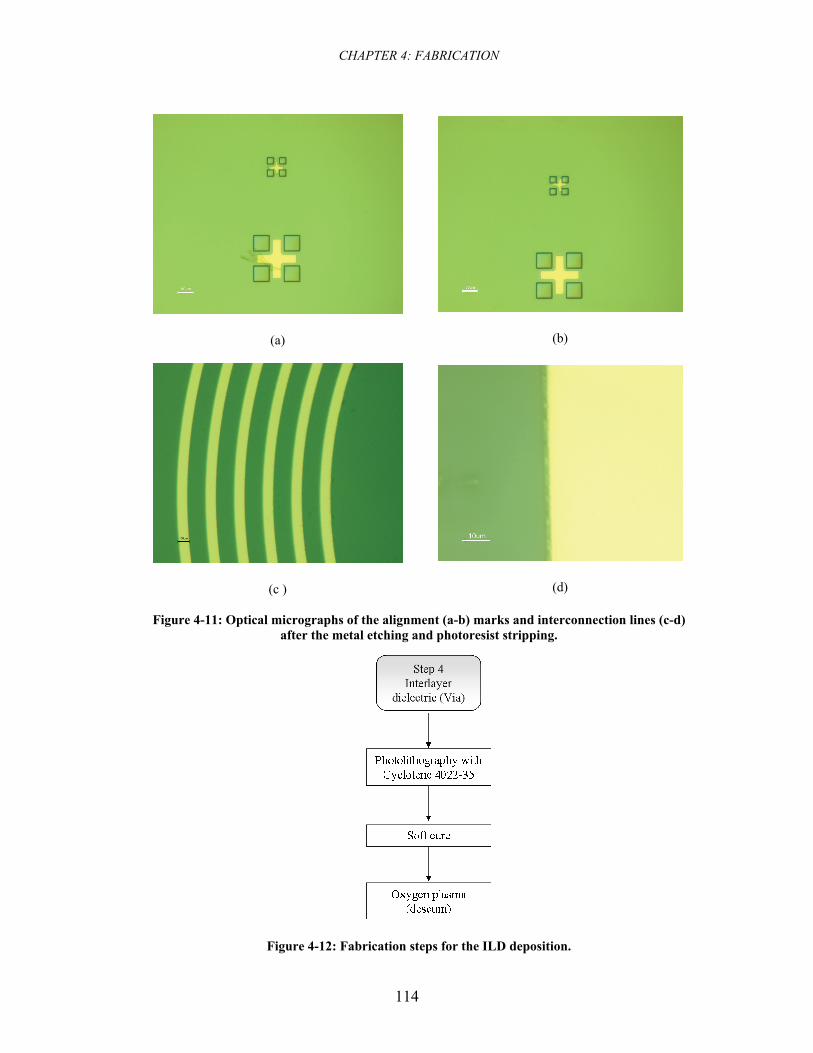
CHAPTER 4: FABRICATION
114
(a)
(b)
(c )
(d)
Figure 4-11: Optical micrographs of the alignment (a-b) marks and interconnection lines (c-d) after the metal etching and photoresist stripping.
Figure 4-12: Fabrication steps for the ILD deposition.
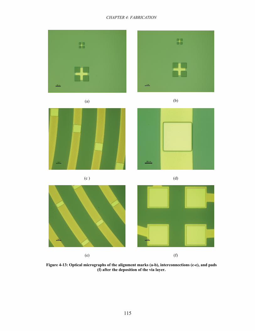
CHAPTER 4: FABRICATION
115
(a)
(b)
(c )
(d)
(e)
(f)
Figure 4-13: Optical micrographs of the alignment marks (a-b), interconnections (c-e), and pads (f) after the deposition of the via layer.
CHAPTER 4: FABRICATION
116
4.3.5 Electrodes
The fabrication process of the electrode layer is different from the interconnection
layer. The lift-off process summarized in Figure 4-14 is used instead of the “etch
process”. Etch process was used for the interconnection layer because the exact
geometry of the lines is not important. However, if a single line is lost due to the
imperfections in the fabrication process, the machine has no longer six phases. The
adhesion loss of the metal film to the BCB layer is highly probable in the lift-off
process30. Therefore, the etch process was used for the first metal layer. For the
electrode layer, however, the precision in the geometry is extremely important.
Therefore, the lift-off process is used.
The fist step is creating a photoresist layer with lift-off profile (angled sidewalls).
This photolithography step is detailed in Table 4-5. Figure 4-15 shows the fabrication
results after photolithography.
Short oxygen plasma is used before metal deposition to remove any photoresist
residues from the via opening areas. This ensures good electrical connection between
the two metal layers. The photoresist etching parameters are summarized in Table
4-2. Similar to the first metal layer, chromium and gold films are sputtered next. The
wafer is then placed inside an acetone solution in an ultrasonic bath (from Bronson)
for 15 min. The acetone solution is renewed followed by another 15 min of ultrason.
Finally, the wafer is rinsed with DI for 30 min in the ultrasonic bath. The purpose of
the latter is to remove any metal residues from the surface. Figure 4-16 shows a
micrograph of the device after the completion of this step.
30 If lift-off process were used for the first metal, eventually the first metal line would go through acetone ultrasonic bath twice (once for each metal layer).
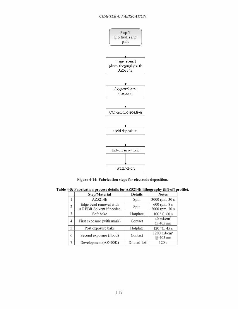
CHAPTER 4: FABRICATION
117
Figure 4-14: Fabrication steps for electrode deposition.
Table 4-5: Fabrication process details for AZ5214E lithography (lift-off profile). Step/Material Details Notes
1 AZ5214E Spin 3000 rpm, 30 s
2 Edge bead removal with AZ EBR Solvent if needed Spin 600 rpm, 8 s
2000 rpm, 30 s 3 Soft bake Hotplate 100 °C, 60 s
4 First exposure (with mask) Contact 40 mJ/cm2 @ 405 nm
5 Post exposure bake Hotplate 120 °C, 45 s
6 Second exposure (flood) Contact 1200 mJ/cm2 @ 405 nm
7 Development (AZ400K) Diluted 1:6 120 s
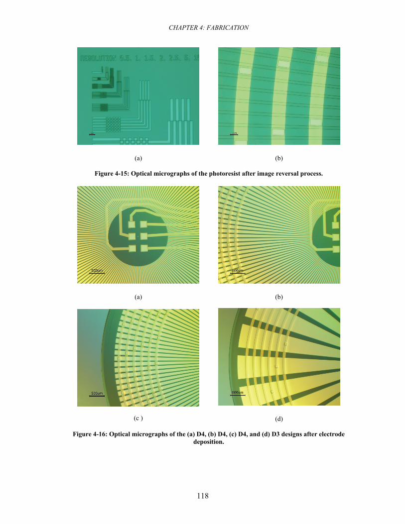
CHAPTER 4: FABRICATION
118
(a)
(b)
Figure 4-15: Optical micrographs of the photoresist after image reversal process.
(a)
(b)
(c )
(d)
Figure 4-16: Optical micrographs of the (a) D4, (b) D4, (c) D4, and (d) D3 designs after electrode deposition.
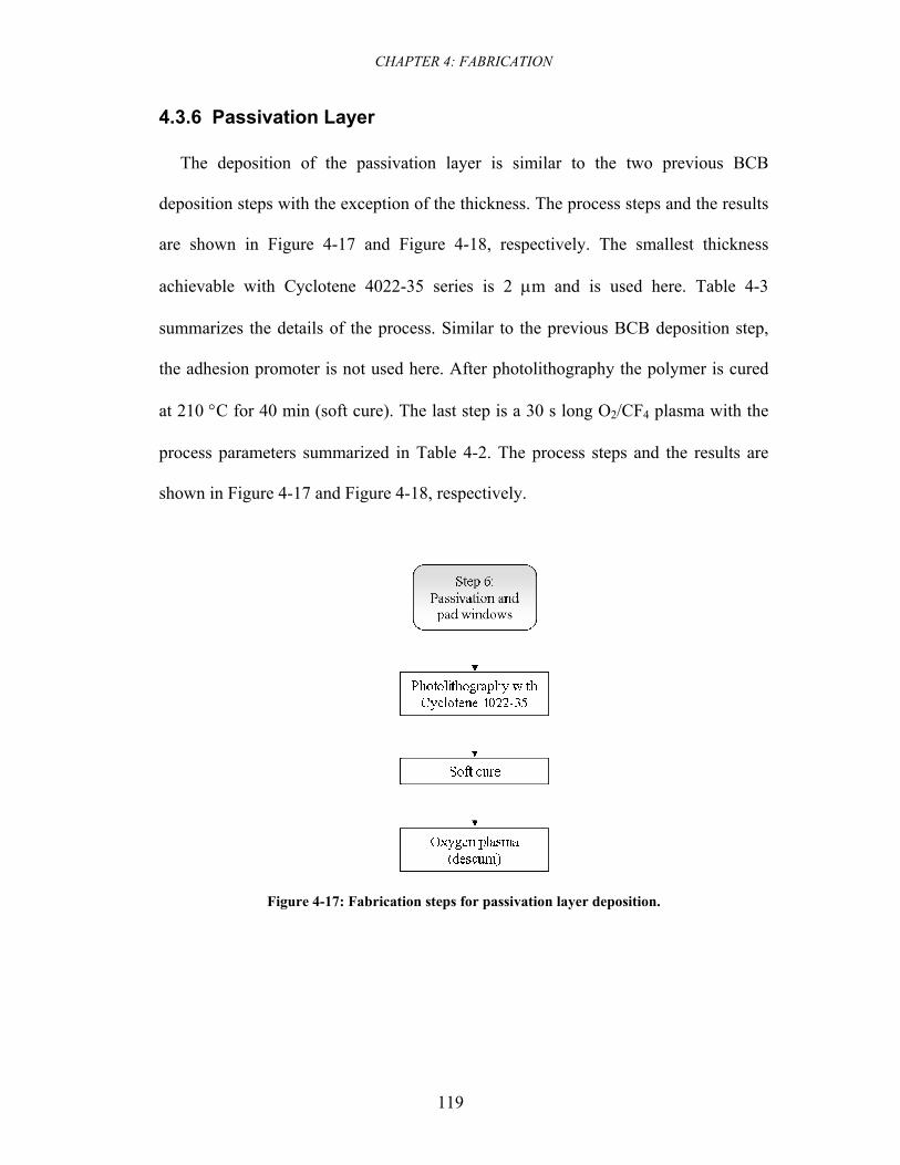
CHAPTER 4: FABRICATION
119
4.3.6 Passivation Layer
The deposition of the passivation layer is similar to the two previous BCB
deposition steps with the exception of the thickness. The process steps and the results
are shown in Figure 4-17 and Figure 4-18, respectively. The smallest thickness
achievable with Cyclotene 4022-35 series is 2 μm and is used here. Table 4-3
summarizes the details of the process. Similar to the previous BCB deposition step,
the adhesion promoter is not used here. After photolithography the polymer is cured
at 210 °C for 40 min (soft cure). The last step is a 30 s long O2/CF4 plasma with the
process parameters summarized in Table 4-2. The process steps and the results are
shown in Figure 4-17 and Figure 4-18, respectively.
Figure 4-17: Fabrication steps for passivation layer deposition.
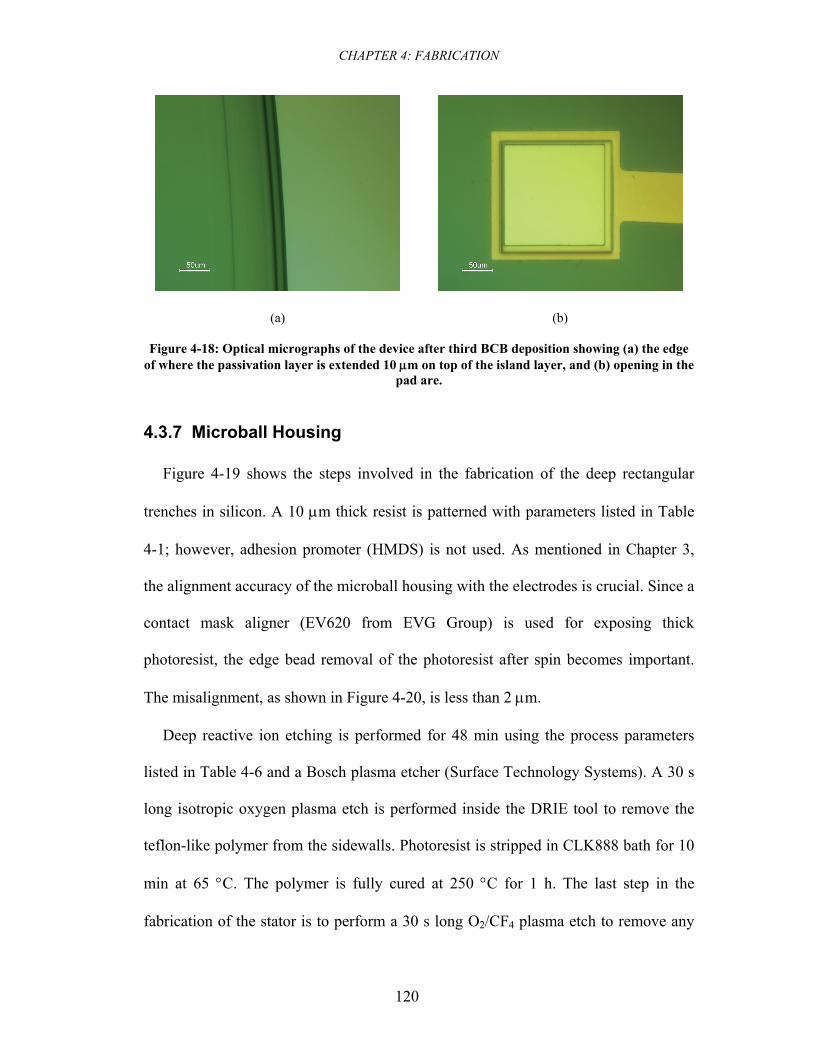
CHAPTER 4: FABRICATION
120
(a)
(b)
Figure 4-18: Optical micrographs of the device after third BCB deposition showing (a) the edge of where the passivation layer is extended 10 μm on top of the island layer, and (b) opening in the
pad are.
4.3.7 Microball Housing
Figure 4-19 shows the steps involved in the fabrication of the deep rectangular
trenches in silicon. A 10 μm thick resist is patterned with parameters listed in Table
4-1; however, adhesion promoter (HMDS) is not used. As mentioned in Chapter 3,
the alignment accuracy of the microball housing with the electrodes is crucial. Since a
contact mask aligner (EV620 from EVG Group) is used for exposing thick
photoresist, the edge bead removal of the photoresist after spin becomes important.
The misalignment, as shown in Figure 4-20, is less than 2 μm.
Deep reactive ion etching is performed for 48 min using the process parameters
listed in Table 4-6 and a Bosch plasma etcher (Surface Technology Systems). A 30 s
long isotropic oxygen plasma etch is performed inside the DRIE tool to remove the
teflon-like polymer from the sidewalls. Photoresist is stripped in CLK888 bath for 10
min at 65 °C. The polymer is fully cured at 250 °C for 1 h. The last step in the
fabrication of the stator is to perform a 30 s long O2/CF4 plasma etch to remove any
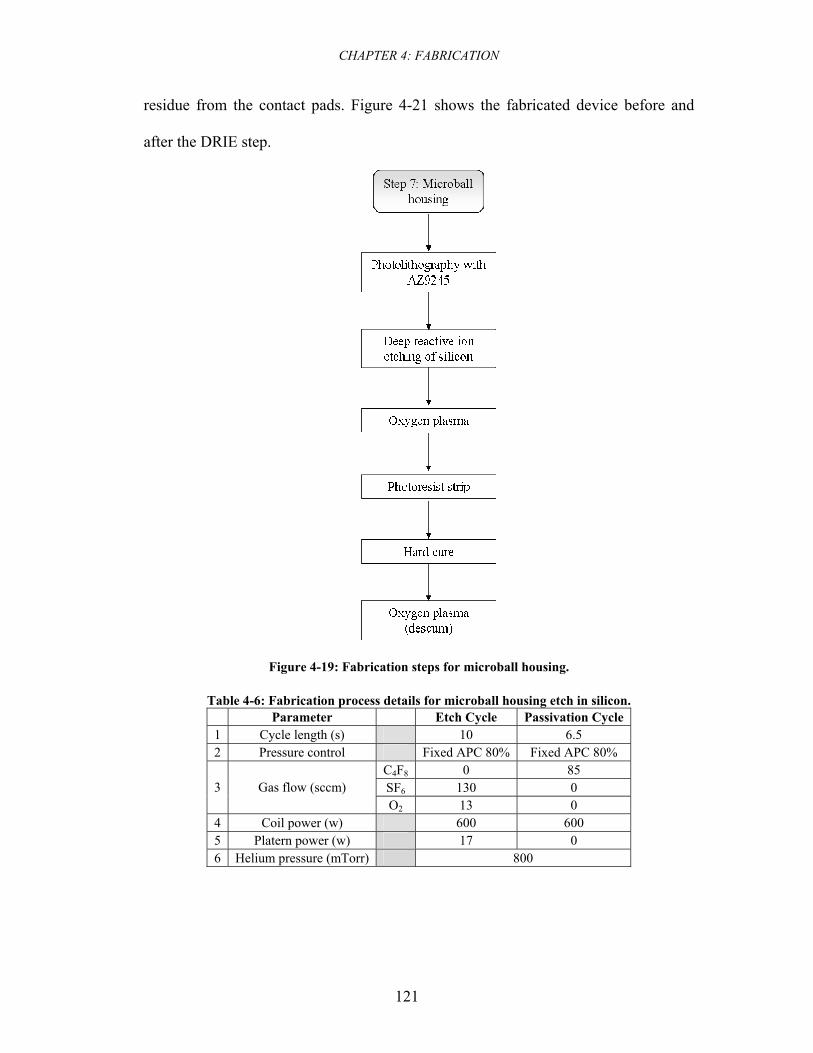
CHAPTER 4: FABRICATION
121
residue from the contact pads. Figure 4-21 shows the fabricated device before and
after the DRIE step.
Figure 4-19: Fabrication steps for microball housing.
Table 4-6: Fabrication process details for microball housing etch in silicon. Parameter Etch Cycle Passivation Cycle 1 Cycle length (s) 10 6.5 2 Pressure control Fixed APC 80% Fixed APC 80%
C4F8 0 85 SF6 130 0 3 Gas flow (sccm) O2 13 0
4 Coil power (w) 600 600 5 Platern power (w) 17 0 6 Helium pressure (mTorr) 800
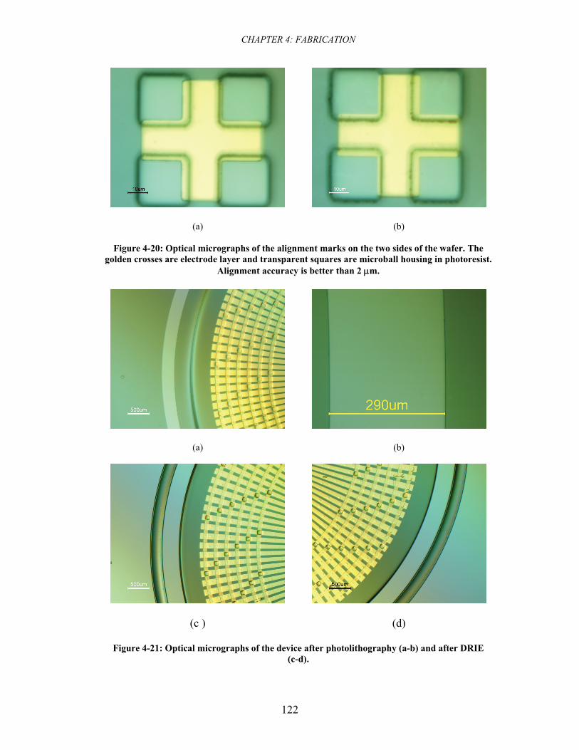
CHAPTER 4: FABRICATION
122
(a)
(b)
Figure 4-20: Optical micrographs of the alignment marks on the two sides of the wafer. The golden crosses are electrode layer and transparent squares are microball housing in photoresist.
Alignment accuracy is better than 2 μm.
(a)
(b)
(c )
(d)
Figure 4-21: Optical micrographs of the device after photolithography (a-b) and after DRIE (c-d).
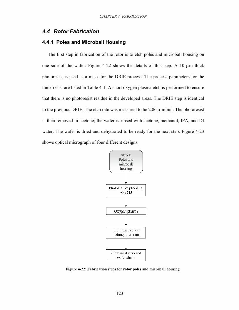
CHAPTER 4: FABRICATION
123
4.4 Rotor Fabrication
4.4.1 Poles and Microball Housing
The first step in fabrication of the rotor is to etch poles and microball housing on
one side of the wafer. Figure 4-22 shows the details of this step. A 10 μm thick
photoresist is used as a mask for the DRIE process. The process parameters for the
thick resist are listed in Table 4-1. A short oxygen plasma etch is performed to ensure
that there is no photoresist residue in the developed areas. The DRIE step is identical
to the previous DRIE. The etch rate was measured to be 2.86 μm/min. The photoresist
is then removed in acetone; the wafer is rinsed with acetone, methanol, IPA, and DI
water. The wafer is dried and dehydrated to be ready for the next step. Figure 4-23
shows optical micrograph of four different designs.
Figure 4-22: Fabrication steps for rotor poles and microball housing.
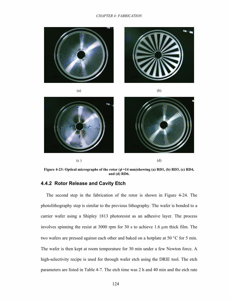
CHAPTER 4: FABRICATION
124
(a)
(b)
(c )
(d)
Figure 4-23: Optical micrographs of the rotor (φ =14 mm)showing (a) RD1, (b) RD3, (c) RD4, and (d) RD6.
4.4.2 Rotor Release and Cavity Etch
The second step in the fabrication of the rotor is shown in Figure 4-24. The
photolithography step is similar to the previous lithography. The wafer is bonded to a
carrier wafer using a Shipley 1813 photoresist as an adhesive layer. The process
involves spinning the resist at 3000 rpm for 30 s to achieve 1.6 μm thick film. The
two wafers are pressed against each other and baked on a hotplate at 50 °C for 5 min.
The wafer is then kept at room temperature for 30 min under a few Newton force. A
high-selectivity recipe is used for through wafer etch using the DRIE tool. The etch
parameters are listed in Table 4-7. The etch time was 2 h and 40 min and the etch rate
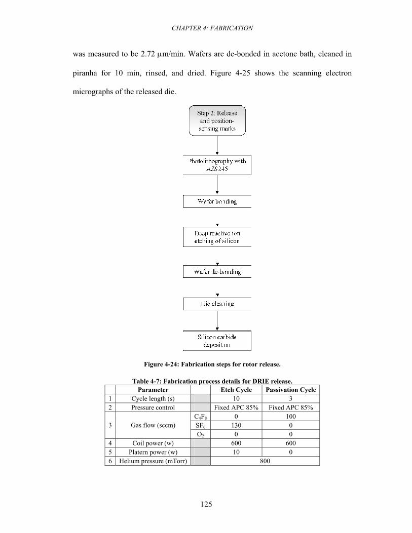
CHAPTER 4: FABRICATION
125
was measured to be 2.72 μm/min. Wafers are de-bonded in acetone bath, cleaned in
piranha for 10 min, rinsed, and dried. Figure 4-25 shows the scanning electron
micrographs of the released die.
Figure 4-24: Fabrication steps for rotor release.
Table 4-7: Fabrication process details for DRIE release. Parameter Etch Cycle Passivation Cycle 1 Cycle length (s) 10 3 2 Pressure control Fixed APC 85% Fixed APC 85%
C4F8 0 100 SF6 130 0 3 Gas flow (sccm) O2 0 0
4 Coil power (w) 600 600 5 Platern power (w) 10 0 6 Helium pressure (mTorr) 800
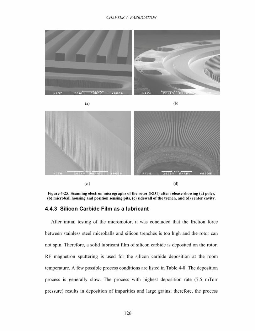
CHAPTER 4: FABRICATION
126
(a) (b)
(c ) (d)
Figure 4-25: Scanning electron micrographs of the rotor (RD1) after release showing (a) poles, (b) microball housing and position sensing pits, (c) sidewall of the trench, and (d) center cavity.
4.4.3 Silicon Carbide Film as a lubricant
After initial testing of the micromotor, it was concluded that the friction force
between stainless steel microballs and silicon trenches is too high and the rotor can
not spin. Therefore, a solid lubricant film of silicon carbide is deposited on the rotor.
RF magnetron sputtering is used for the silicon carbide deposition at the room
temperature. A few possible process conditions are listed in Table 4-8. The deposition
process is generally slow. The process with highest deposition rate (7.5 mTorr
pressure) results in deposition of impurities and large grains; therefore, the process
CHAPTER 4: FABRICATION
127
with the second highest rate (2.5 mTorr pressure) is used. With the total deposition
time of 1 h the estimated silicon carbide thickness is 173 nm.
Table 4-8: Silicon carbide sputtering conditions.
Target Power supply Pressure (mTorr)
Carrier gas, flow (sccm)
Power (W)
Bias (W)
Deposition rate (A/min per
watt) Silicon carbide RF 2.5 Ar, 20 300 300 5.7 Silicon carbide RF 5 Ar, 20 200 200 4 Silicon carbide RF 7.5 Ar, 20 300 300 6.3
4.5 Micromachine Assembly
After the fabrication of the stator and rotor, the stator is clamped (fixed) on an
aluminum chuck. The stainless steel microballs are then manually positioned inside
the stator trench using fine-tip tweezers. The rotor is then manually aligned and
positioned on top of the rotor using tweezers. If the rotor is aligned and positioned
properly, it rotates freely with little resistance.
4.6 Fabrication Summary
The thickness of each layer is measured using a contact or optical profilometer. A
summary of the layer thickness or etch depth for all steps is listed in Table 4-9. The
scanned profiles for the stator and rotor are shown in Figure 4-26 and Figure 4-27,
respectively. Figure 4-26(a) shows the profile of the island after softcure and descum.
The final thickness of the film is given in Table 4-9 which is 10 % smaller due to film
shrinkage during hard cure step. Figure (b) and (d) the interconnection and electrode
layer profiles, respectively, with the thickness of 0.26 μm. Figure (c) and (e) show the
profile of the second and third BCB layers, respectively. The thickness of the first
BCB layers before hard cure were measured to be 3.6, 3.1, and 2.2 μm, respectively.
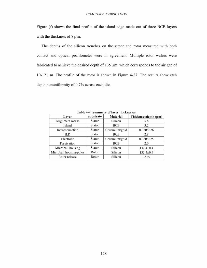
CHAPTER 4: FABRICATION
128
Figure (f) shows the final profile of the island edge made out of three BCB layers
with the thickness of 8 μm.
The depths of the silicon trenches on the stator and rotor measured with both
contact and optical profilometer were in agreement. Multiple rotor wafers were
fabricated to achieve the desired depth of 135 μm, which corresponds to the air gap of
10-12 μm. The profile of the rotor is shown in Figure 4-27. The results show etch
depth nonuniformity of 0.7% across each die.
Table 4-9: Summary of layer thicknesses. Layer Substrate Material Thickness/depth (μm)
Alignment marks Stator Silicon 5.8 Island Stator BCB 3.2
Interconnection Stator Chromium/gold 0.020/0.26 ILD Stator BCB 2.8
Electrode Stator Chromium/gold 0.020/0.25 Passivation Stator BCB 2.0
Microball housing Stator Silicon 132.4±0.4 Microball housing/poles Rotor Silicon 135.5±0.4
Rotor release Rotor Silicon ∼525
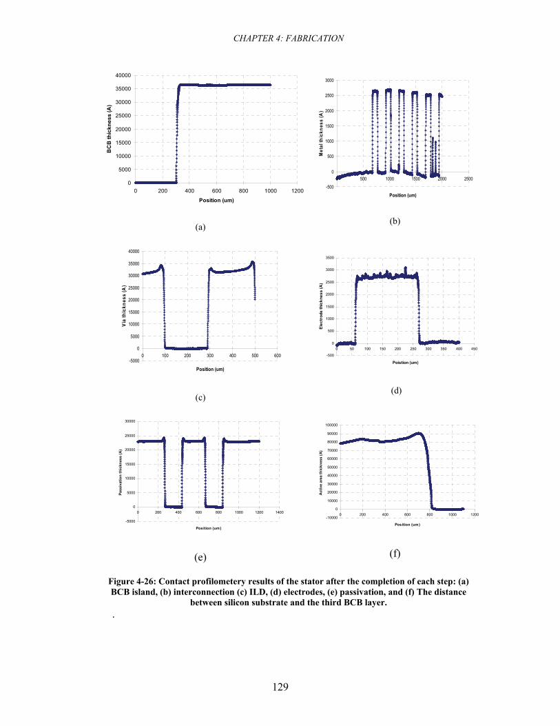
CHAPTER 4: FABRICATION
129
0
5000
10000
15000
20000
25000
30000
35000
40000
0 200 400 600 800 1000 1200
Position (um)
BC
B th
ickn
ess
(A)
(a)
-500
0
500
1000
1500
2000
2500
3000
0 500 1000 1500 2000 2500
Position (um)
Met
al th
ickn
ess
(A)
(b)
-5000
0
5000
10000
15000
20000
25000
30000
35000
40000
0 100 200 300 400 500 600
Position (um)
Via
thic
knes
s (A
)
(c)
-500
0
500
1000
1500
2000
2500
3000
3500
0 50 100 150 200 250 300 350 400 450
Poistion (um)
Elec
trod
e th
ickn
ess
(A)
(d)
-5000
0
5000
10000
15000
20000
25000
30000
0 200 400 600 800 1000 1200 1400
Position (um)
Pass
ivat
ion
thic
knes
s (A
)
(e)
-10000
0
10000
20000
30000
40000
50000
60000
70000
80000
90000
100000
0 200 400 600 800 1000 1200
Position (um)
Act
ive
area
thic
knes
s (A
)
(f)
Figure 4-26: Contact profilometery results of the stator after the completion of each step: (a) BCB island, (b) interconnection (c) ILD, (d) electrodes, (e) passivation, and (f) The distance
between silicon substrate and the third BCB layer. .
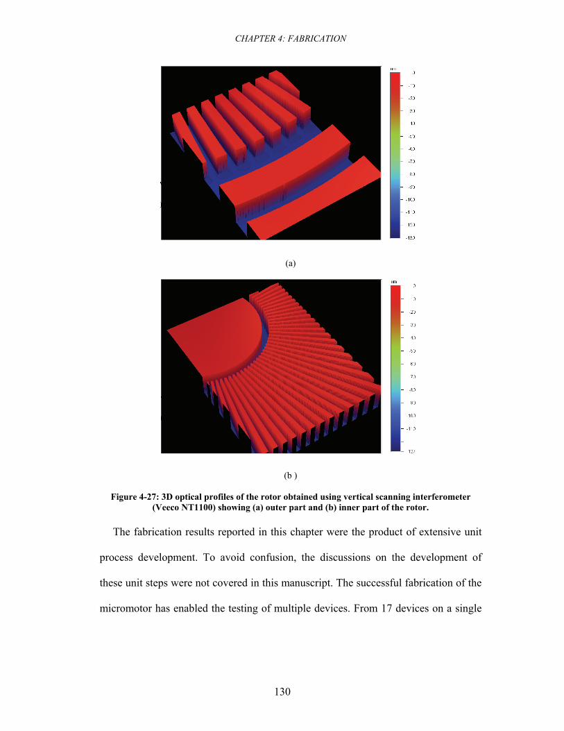
CHAPTER 4: FABRICATION
130
(a)
(b )
Figure 4-27: 3D optical profiles of the rotor obtained using vertical scanning interferometer (Veeco NT1100) showing (a) outer part and (b) inner part of the rotor.
The fabrication results reported in this chapter were the product of extensive unit
process development. To avoid confusion, the discussions on the development of
these unit steps were not covered in this manuscript. The successful fabrication of the
micromotor has enabled the testing of multiple devices. From 17 devices on a single
CHAPTER 4: FABRICATION
131
stator wafer, 15 are testable. The characterization of the fabricated devices is
discussed in Chapter 5.
CHAPTER 5: CHARACTERIZATION
132
5 Characterization
The development of the rotary micromotor is based on the previous work on the
design, fabrication, and testing of the linear micromotors. The rotary micromotor was
extensively discussed in Chapter 1 through 4. In Section 5.1, however, the work
preceding the development of the rotary device is reported. This work has been an
essential backbone for the evolution of the rotary machine. The characterization
results for the linear device are discussed first. In the second part of this chapter
(Section 5.2), the characterization results for the rotary device are reported.
5.1 Linear Micromotor Characterization
5.1.1 Introduction
The primary application of the bottom-drive linear variable-capacitance
micromotor (B-LVCM) is long-range, high-speed, linear micropositioning. In
addition, this device provides a platform to investigate the mechanical properties of
roller bearings in MEMS and learn how to design, fabricate, and test the rotary
micromotor. The detailed design and fabrication, as well as initial test results for the
first-generation 6-phase B-LVCM, were previously reported [130, 131].
The fabrication of the second-generation B-LVCM together with the dynamic
characterization is reported in this chapter. The design and fabrication are described
first, and the test setup used for the characterization is introduced next. The dynamic
characterization including the measurement results of position, instantaneous
velocity, acceleration, and the net force on the slider [132], are presented. The device
is modeled as a simple mass-dashpot-spring system. The model parameters were
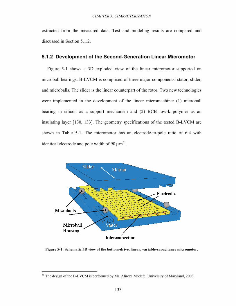
CHAPTER 5: CHARACTERIZATION
133
extracted from the measured data. Test and modeling results are compared and
discussed in Section 5.1.2.
5.1.2 Development of the Second-Generation Linear Micromotor
Figure 5-1 shows a 3D exploded view of the linear micromotor supported on
microball bearings. B-LVCM is comprised of three major components: stator, slider,
and microballs. The slider is the linear counterpart of the rotor. Two new technologies
were implemented in the development of the linear micromachine: (1) microball
bearing in silicon as a support mechanism and (2) BCB low-k polymer as an
insulating layer [130, 133]. The geometry specifications of the tested B-LVCM are
shown in Table 5-1. The micromotor has an electrode-to-pole ratio of 6:4 with
identical electrode and pole width of 90 μm31.
Figure 5-1: Schematic 3D view of the bottom-drive, linear, variable-capacitance micromotor.
31 The design of the B-LVCM is performed by Mr. Alireza Modafe, University of Maryland, 2003.
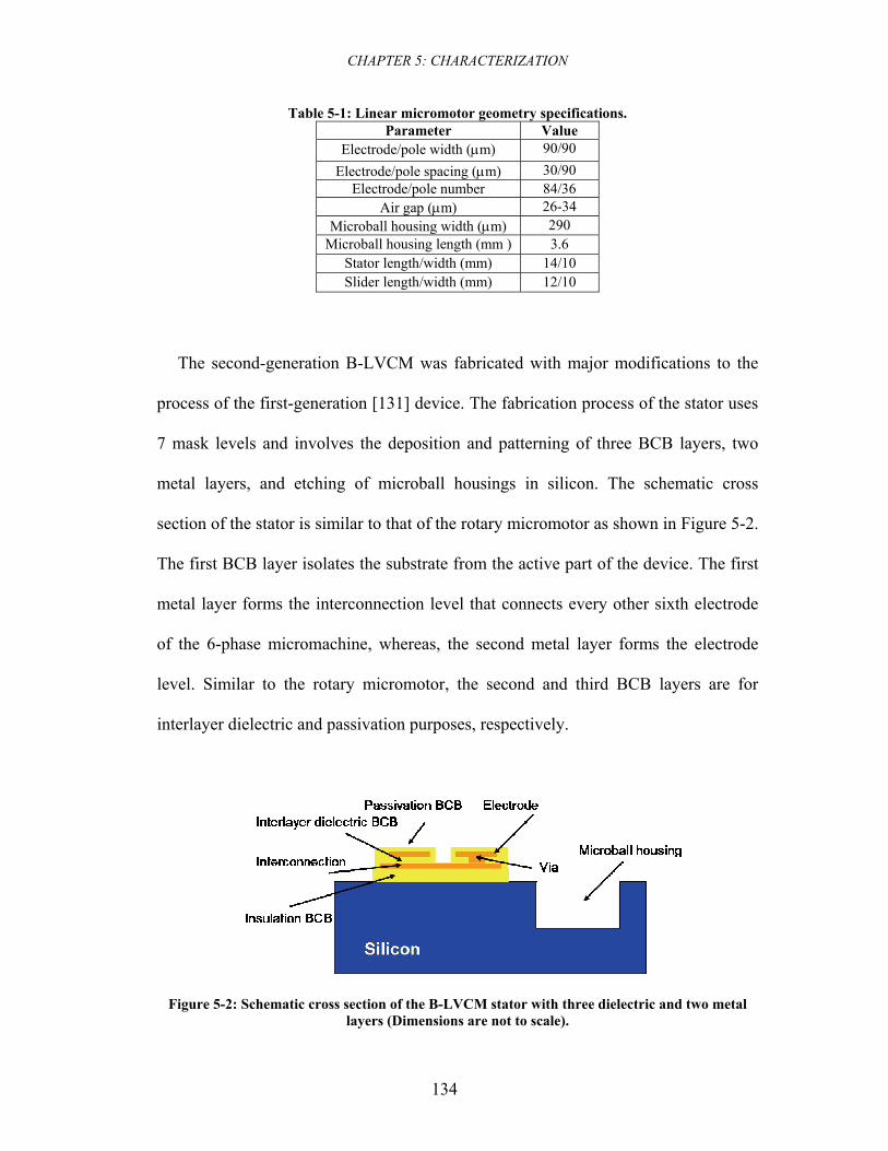
CHAPTER 5: CHARACTERIZATION
134
Table 5-1: Linear micromotor geometry specifications. Parameter Value
Electrode/pole width (μm) 90/90 Electrode/pole spacing (μm) 30/90
Electrode/pole number 84/36 Air gap (μm) 26-34
Microball housing width (μm) 290 Microball housing length (mm ) 3.6
Stator length/width (mm) 14/10 Slider length/width (mm) 12/10
The second-generation B-LVCM was fabricated with major modifications to the
process of the first-generation [131] device. The fabrication process of the stator uses
7 mask levels and involves the deposition and patterning of three BCB layers, two
metal layers, and etching of microball housings in silicon. The schematic cross
section of the stator is similar to that of the rotary micromotor as shown in Figure 5-2.
The first BCB layer isolates the substrate from the active part of the device. The first
metal layer forms the interconnection level that connects every other sixth electrode
of the 6-phase micromachine, whereas, the second metal layer forms the electrode
level. Similar to the rotary micromotor, the second and third BCB layers are for
interlayer dielectric and passivation purposes, respectively.
Figure 5-2: Schematic cross section of the B-LVCM stator with three dielectric and two metal layers (Dimensions are not to scale).
CHAPTER 5: CHARACTERIZATION
135
First, a 3 μm thick photosensitive BCB (Cyclotene 4024-40 from Dow Chemical)
is spun, patterned, and partially cured (at 210 °C for 50 min). In the first-generation
device [131] this step included a silicon etch step (30 μm deep) using DRIE and
multiple photolithography and chemical mechanical planarization (CMP) steps. For
simplicity, those steps were replaced by a 3 μm thick BCB deposition. The drawback
of this process is smaller thickness for the isolation layer. Consequently, a higher
parasitic capacitance and lower efficiency device is attained. The advantage of this
process is less fabrication complexity, higher yield, and shorter process time.
A 20/250 nm thick Cr/Au metal layer (interconnection) is then sputtered and
patterned using a positive photoresist (Shipley 1813) and wet etching. The yield of
the Cr/Au metallization process was increased by replacing the original lift-off
process, in the first-generation device, with an etch process. The original lift-off
process resulted in the partial loss of interconnection layer. This phenomenon reduces
the number of active phases of the machine.
A dielectric layer (Cyclotene 4024-40) with a thickness of 3.2 μm is then spun,
patterned, and partially cured (at 210 °C for 50 min) to form an interlayer dielectric
(ILD) with open vias for electrical connection between the two metal layers. The
partial cure of the BCB results in 75 % polymerization and a better adhesion to the
metal layers [93]. The thickness of this layer was increased from 2 μm in the first-
generation device to 3.2 μm to provide more uniform step coverage and higher
breakdown voltage.
CHAPTER 5: CHARACTERIZATION
136
The second metal layer (electrode) with 20/250 nm thick Cr/Au layer is patterned
using photolithography with an image reversal photoresist (AZ5214E), sputtering,
and lift-off in acetone. A 2.1 μm thick passivation layer (Cyclotene 4022-35) is then
spun, patterned, and fully cured (at 250 °C for 1 h). This is followed by the patterning
and etching of silicon (130 μm deep) using a 9 μm thick positive photoresist
(AZ9245) and DRIE to form the microball housings. The process details for each step
are similar to ones reported in Chapter 4 for the rotary device. Figure 5-3 shows the
optical micrograph of the stator at different fabrication steps.
The slider fabrication process is comprised of a lithography step and a DRIE step
to etch microball housing and poles simultaneously. Figure 5-4 and Figure 5-5 show
the fabricated stator and slider of the 6-phase micromotor, respectively. The assembly
of the micromotor requires the manual placement of the microballs in the stator
trenches using a pair of tweezers. The slider is then aligned with the stator and
positioned on top of the microballs.
5.1.3 Test Setup
A test-bed for the characterization of the micromotor was developed. Figure 5-6
shows the block diagram of the test station consisting of a 6-channel, high-voltage
actuation system, a high-speed camera, and an image processing unit. Initially, the
motion of the motor was captured using a 30-frame-per-second (fps) camera (Model
DCR-HC42 from Sony) and a microscopic lens (35 mm, 24×).
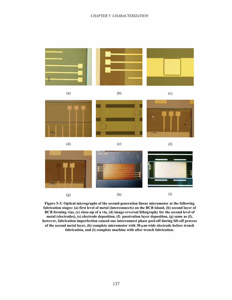
CHAPTER 5: CHARACTERIZATION
137
(a) (b)
(c)
(d)
(e)
(f)
(g)
(h)
(i)
Figure 5-3: Optical micrographs of the second-generation linear micromotor at the following fabrication stages: (a) first level of metal (interconnects) on the BCB island, (b) second layer of BCB forming vias, (c) close-up of a via, (d) image-reversal lithography for the second level of metal (electrodes), (e) electrode deposition, (f) passivation layer deposition, (g) same as (f),
however, fabrication imperfection caused one interconnect phase peel-off during lift-off process of the second metal layer, (h) complete micromotor with 30-μm-wide electrode before trench
fabrication, and (i) complete machine with after trench fabrication.
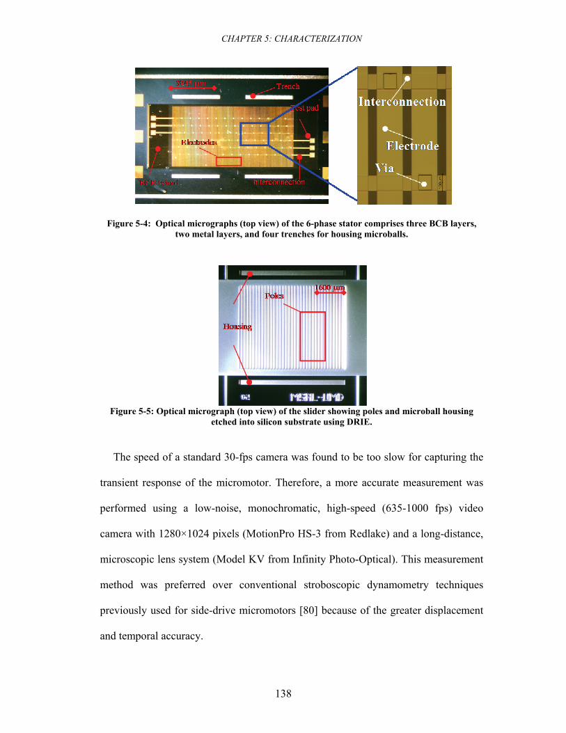
CHAPTER 5: CHARACTERIZATION
138
Figure 5-4: Optical micrographs (top view) of the 6-phase stator comprises three BCB layers, two metal layers, and four trenches for housing microballs.
Figure 5-5: Optical micrograph (top view) of the slider showing poles and microball housing
etched into silicon substrate using DRIE.
The speed of a standard 30-fps camera was found to be too slow for capturing the
transient response of the micromotor. Therefore, a more accurate measurement was
performed using a low-noise, monochromatic, high-speed (635-1000 fps) video
camera with 1280×1024 pixels (MotionPro HS-3 from Redlake) and a long-distance,
microscopic lens system (Model KV from Infinity Photo-Optical). This measurement
method was preferred over conventional stroboscopic dynamometry techniques
previously used for side-drive micromotors [80] because of the greater displacement
and temporal accuracy.
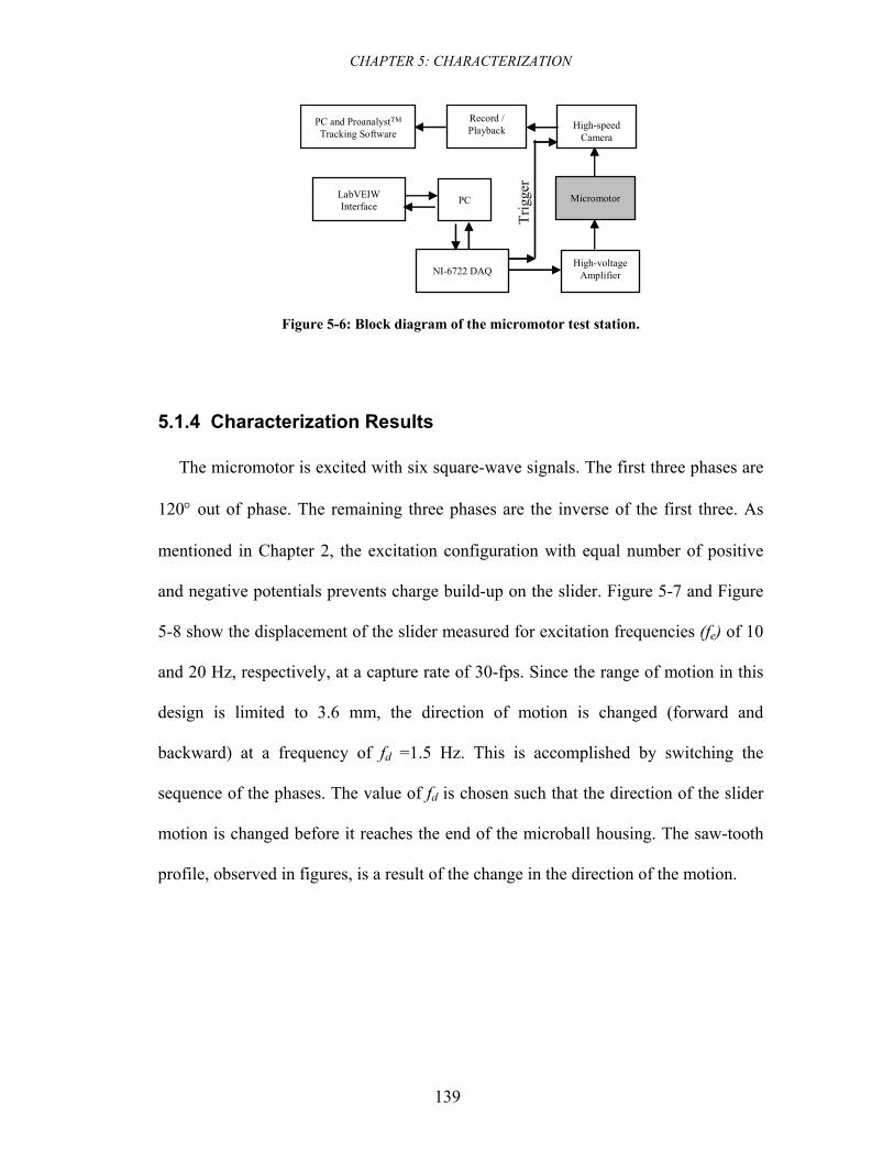
CHAPTER 5: CHARACTERIZATION
139
PC and ProanalystTM
Tracking SoftwareRecord / Playback High-speed
Camera
LabVEIWInterface PC Micromotor
NI-6722 DAQHigh-voltage
Amplifier
Trig
ger
Figure 5-6: Block diagram of the micromotor test station.
5.1.4 Characterization Results
The micromotor is excited with six square-wave signals. The first three phases are
120° out of phase. The remaining three phases are the inverse of the first three. As
mentioned in Chapter 2, the excitation configuration with equal number of positive
and negative potentials prevents charge build-up on the slider. Figure 5-7 and Figure
5-8 show the displacement of the slider measured for excitation frequencies (fe) of 10
and 20 Hz, respectively, at a capture rate of 30-fps. Since the range of motion in this
design is limited to 3.6 mm, the direction of motion is changed (forward and
backward) at a frequency of fd =1.5 Hz. This is accomplished by switching the
sequence of the phases. The value of fd is chosen such that the direction of the slider
motion is changed before it reaches the end of the microball housing. The saw-tooth
profile, observed in figures, is a result of the change in the direction of the motion.
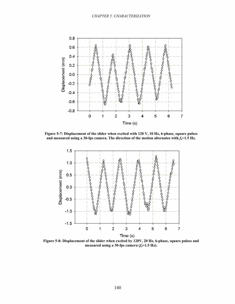
CHAPTER 5: CHARACTERIZATION
140
Figure 5-7: Displacement of the slider when excited with 120 V, 10 Hz, 6-phase, square pulses and measured using a 30-fps camera. The direction of the motion alternates with fd=1.5 Hz.
Figure 5-8: Displacement of the slider when excited by 120V, 20 Hz, 6-phase, square pulses and
measured using a 30-fps camera (fd=1.5 Hz).
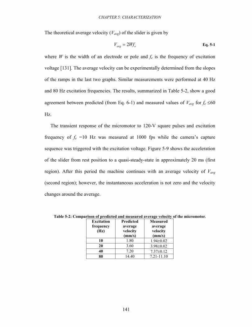
CHAPTER 5: CHARACTERIZATION
141
The theoretical average velocity (Vavg) of the slider is given by
eavg WfV 2= Eq. 5-1
where W is the width of an electrode or pole and fe is the frequency of excitation
voltage [131]. The average velocity can be experimentally determined from the slopes
of the ramps in the last two graphs. Similar measurements were performed at 40 Hz
and 80 Hz excitation frequencies. The results, summarized in Table 5-2, show a good
agreement between predicted (from Eq. 6-1) and measured values of Vavg for fe ≤60
Hz.
The transient response of the micromotor to 120-V square pulses and excitation
frequency of fe =10 Hz was measured at 1000 fps while the camera’s capture
sequence was triggered with the excitation voltage. Figure 5-9 shows the acceleration
of the slider from rest position to a quasi-steady-state in approximately 20 ms (first
region). After this period the machine continues with an average velocity of Vavg
(second region); however, the instantaneous acceleration is not zero and the velocity
changes around the average.
Table 5-2: Comparison of predicted and measured average velocity of the micromotor. Excitation frequency
(Hz)
Predicted average velocity (mm/s)
Measured average velocity (mm/s)
10 1.80 1.94±0.02 20 3.60 3.98±0.02 40 7.20 7.37±0.12 80 14.40 7.21-11.10
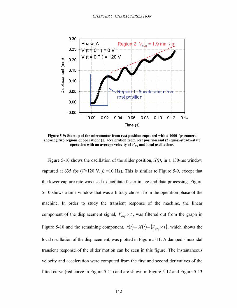
CHAPTER 5: CHARACTERIZATION
142
Figure 5-9: Startup of the micromotor from rest position captured with a 1000-fps camera showing two regions of operation: (1) acceleration from rest position and (2) quasi-steady-state
operation with an average velocity of Vavg and local oscillations.
Figure 5-10 shows the oscillation of the slider position, X(t), in a 130-ms window
captured at 635 fps (V=120 V, fe =10 Hz). This is similar to Figure 5-9, except that
the lower capture rate was used to facilitate faster image and data processing. Figure
5-10 shows a time window that was arbitrary chosen from the operation phase of the
machine. In order to study the transient response of the machine, the linear
component of the displacement signal, tVavg × , was filtered out from the graph in
Figure 5-10 and the remaining component, ( ) ( ) ( )tVtXtx avg ×−= , which shows the
local oscillation of the displacement, was plotted in Figure 5-11. A damped sinusoidal
transient response of the slider motion can be seen in this figure. The instantaneous
velocity and acceleration were computed from the first and second derivatives of the
fitted curve (red curve in Figure 5-11) and are shown in Figure 5-12 and Figure 5-13
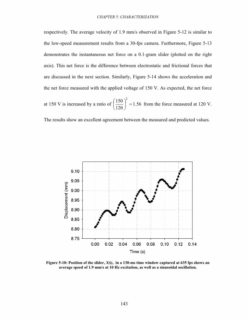
CHAPTER 5: CHARACTERIZATION
143
respectively. The average velocity of 1.9 mm/s observed in Figure 5-12 is similar to
the low-speed measurement results from a 30-fps camera. Furthermore, Figure 5-13
demonstrates the instantaneous net force on a 0.1-gram slider (plotted on the right
axis). This net force is the difference between electrostatic and frictional forces that
are discussed in the next section. Similarly, Figure 5-14 shows the acceleration and
the net force measured with the applied voltage of 150 V. As expected, the net force
at 150 V is increased by a ratio of 56.1120150 2
=⎟⎠⎞
⎜⎝⎛ from the force measured at 120 V.
The results show an excellent agreement between the measured and predicted values.
Figure 5-10: Position of the slider, X(t), in a 130-ms time window captured at 635 fps shows an average speed of 1.9 mm/s at 10 Hz excitation, as well as a sinusoidal oscillation.
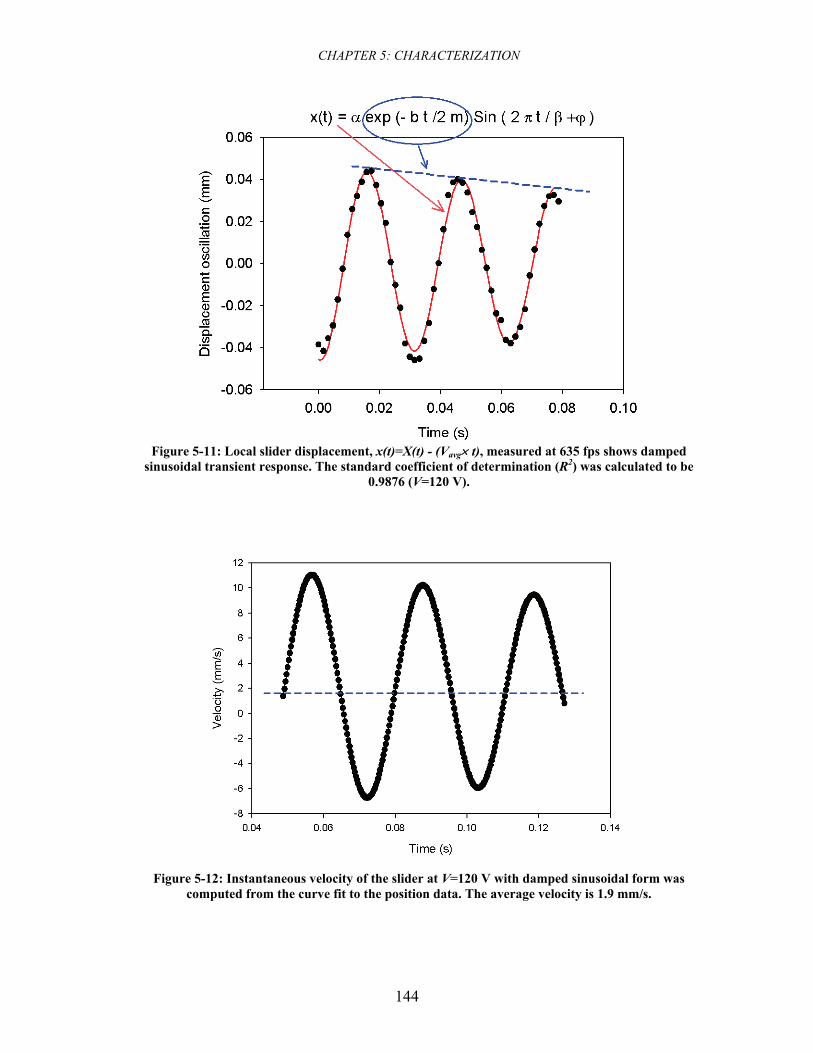
CHAPTER 5: CHARACTERIZATION
144
Figure 5-11: Local slider displacement, x(t)=X(t) - (Vavg× t), measured at 635 fps shows damped
sinusoidal transient response. The standard coefficient of determination (R2) was calculated to be 0.9876 (V=120 V).
Figure 5-12: Instantaneous velocity of the slider at V=120 V with damped sinusoidal form was
computed from the curve fit to the position data. The average velocity is 1.9 mm/s.
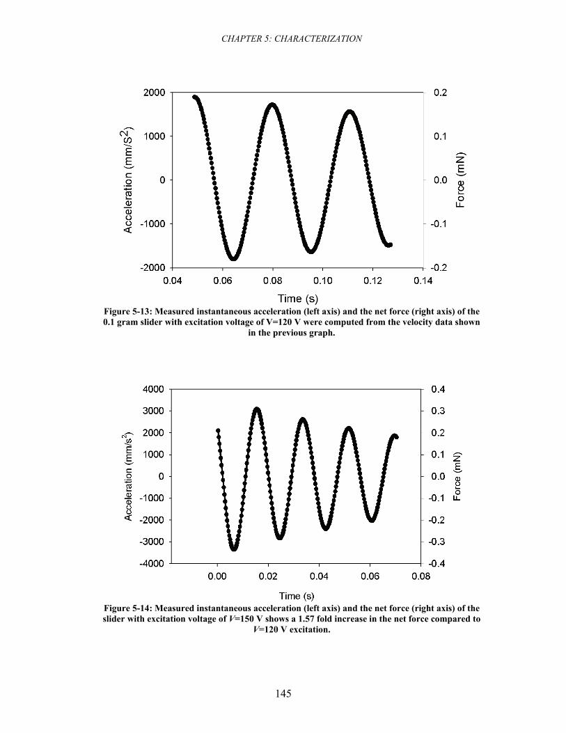
CHAPTER 5: CHARACTERIZATION
145
Figure 5-13: Measured instantaneous acceleration (left axis) and the net force (right axis) of the 0.1 gram slider with excitation voltage of V=120 V were computed from the velocity data shown
in the previous graph.
Figure 5-14: Measured instantaneous acceleration (left axis) and the net force (right axis) of the slider with excitation voltage of V=150 V shows a 1.57 fold increase in the net force compared to
V=120 V excitation.
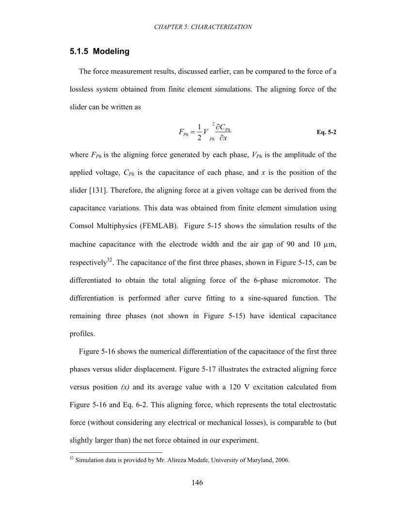
CHAPTER 5: CHARACTERIZATION
146
5.1.5 Modeling
The force measurement results, discussed earlier, can be compared to the force of a
lossless system obtained from finite element simulations. The aligning force of the
slider can be written as
xCVF Ph
PhPh ∂
∂=
2
21
Eq. 5-2
where FPh is the aligning force generated by each phase, VPh is the amplitude of the
applied voltage, CPh is the capacitance of each phase, and x is the position of the
slider [131]. Therefore, the aligning force at a given voltage can be derived from the
capacitance variations. This data was obtained from finite element simulation using
Comsol Multiphysics (FEMLAB). Figure 5-15 shows the simulation results of the
machine capacitance with the electrode width and the air gap of 90 and 10 μm,
respectively32. The capacitance of the first three phases, shown in Figure 5-15, can be
differentiated to obtain the total aligning force of the 6-phase micromotor. The
differentiation is performed after curve fitting to a sine-squared function. The
remaining three phases (not shown in Figure 5-15) have identical capacitance
profiles.
Figure 5-16 shows the numerical differentiation of the capacitance of the first three
phases versus slider displacement. Figure 5-17 illustrates the extracted aligning force
versus position (x) and its average value with a 120 V excitation calculated from
Figure 5-16 and Eq. 6-2. This aligning force, which represents the total electrostatic
force (without considering any electrical or mechanical losses), is comparable to (but
slightly larger than) the net force obtained in our experiment. 32 Simulation data is provided by Mr. Alireza Modafe, University of Maryland, 2006.
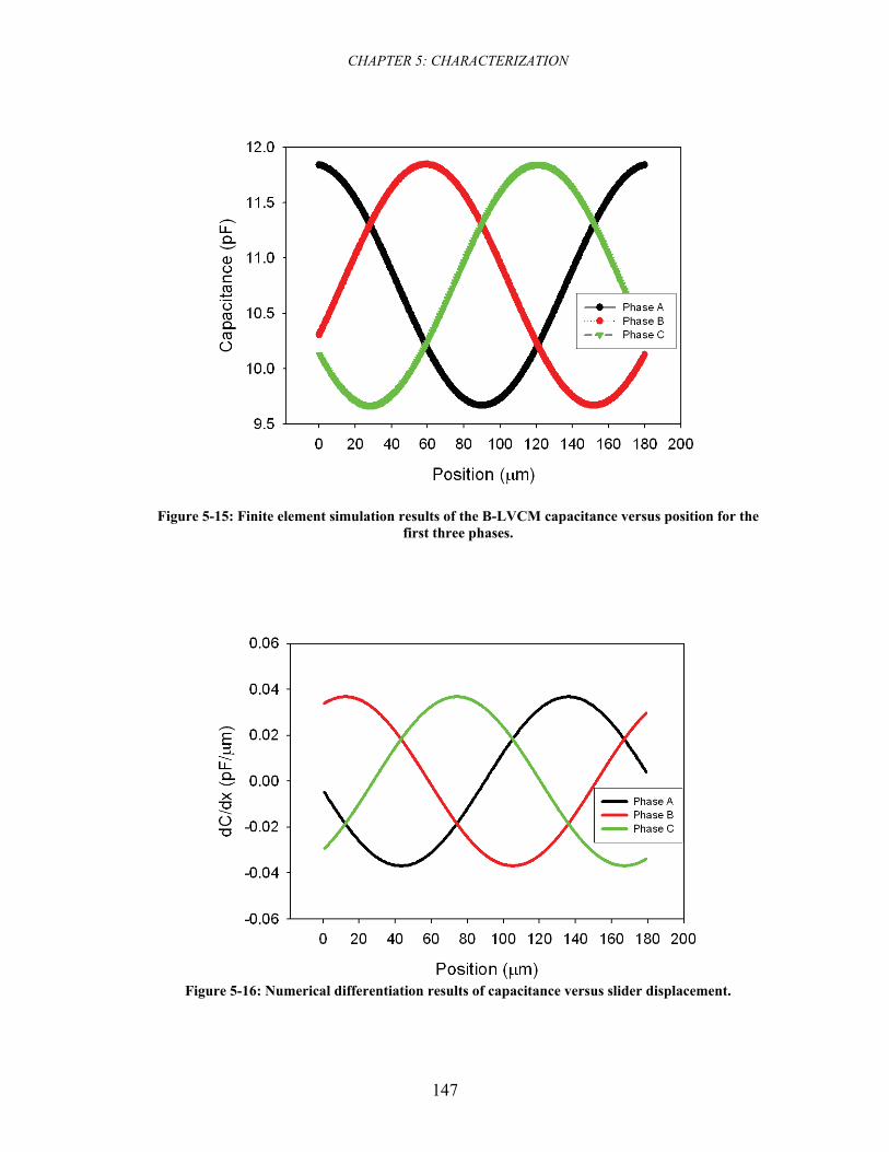
CHAPTER 5: CHARACTERIZATION
147
Figure 5-15: Finite element simulation results of the B-LVCM capacitance versus position for the first three phases.
Figure 5-16: Numerical differentiation results of capacitance versus slider displacement.
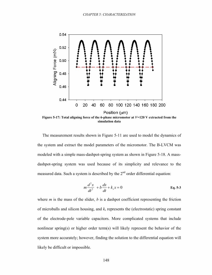
CHAPTER 5: CHARACTERIZATION
148
Figure 5-17: Total aligning force of the 6-phase micromotor at V=120 V extracted from the
simulation data
The measurement results shown in Figure 5-11 are used to model the dynamics of
the system and extract the model parameters of the micromotor. The B-LVCM was
modeled with a simple mass-dashpot-spring system as shown in Figure 5-18. A mass-
dashpot-spring system was used because of its simplicity and relevance to the
measured data. Such a system is described by the 2nd order differential equation:
02
2
=++ xkdtdxb
dtxdm s Eq. 5-3
where m is the mass of the slider, b is a dashpot coefficient representing the friction
of microballs and silicon housing, and ks represents the (electrostatic) spring constant
of the electrode-pole variable capacitors. More complicated systems that include
nonlinear spring(s) or higher order term(s) will likely represent the behavior of the
system more accurately; however, finding the solution to the differential equation will
likely be difficult or impossible.
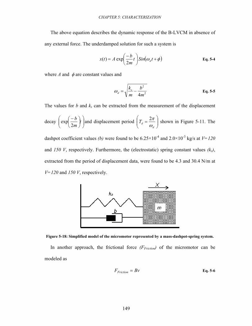
CHAPTER 5: CHARACTERIZATION
149
The above equation describes the dynamic response of the B-LVCM in absence of
any external force. The underdamped solution for such a system is
( )φω +⎟⎠⎞
⎜⎝⎛ −
= tSintmbAtx d2
exp)( Eq. 5-4
where A and φ are constant values and
2
2
4mb
mks
d −=ω Eq. 5-5
The values for b and ks can be extracted from the measurement of the displacement
decay ⎟⎟⎠
⎞⎜⎜⎝
⎛⎟⎠⎞
⎜⎝⎛ − t
mb
2exp and displacement period ⎟⎟
⎠
⎞⎜⎜⎝
⎛=
ddT
ωπ2 shown in Figure 5-11. The
dashpot coefficient values (b) were found to be 6.25×10⁻⁴ and 2.0×10⁻³ kg/s at V=120
and 150 V, respectively. Furthermore, the (electrostatic) spring constant values (ks),
extracted from the period of displacement data, were found to be 4.3 and 30.4 N/m at
V=120 and 150 V, respectively.
Figure 5-18: Simplified model of the micromotor represented by a mass-dashpot-spring system.
In another approach, the frictional force (FFriction) of the micromotor can be
modeled as
BvFFriction = Eq. 5-6
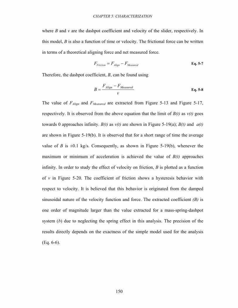
CHAPTER 5: CHARACTERIZATION
150
where B and v are the dashpot coefficient and velocity of the slider, respectively. In
this model, B is also a function of time or velocity. The frictional force can be written
in terms of a theoretical aligning force and net measured force.
MeasuredAlignFriction FFF −= Eq. 5-7
Therefore, the dashpot coefficient, B, can be found using
vFF
B MeasuredAlign −= Eq. 5-8
The value of FAlign and FMeasured are extracted from Figure 5-13 and Figure 5-17,
respectively. It is observed from the above equation that the limit of B(t) as v(t) goes
towards 0 approaches infinity. B(t) as v(t) are shown in Figure 5-19(a); B(t) and a(t)
are shown in Figure 5-19(b). It is observed that for a short range of time the average
value of B is ±0.1 kg/s. Consequently, as shown in Figure 5-19(b), whenever the
maximum or minimum of acceleration is achieved the value of B(t) approaches
infinity. In order to study the effect of velocity on friction, B is plotted as a function
of v in Figure 5-20. The coefficient of friction shows a hysteresis behavior with
respect to velocity. It is believed that this behavior is originated from the damped
sinusoidal nature of the velocity function and force. The extracted coefficient (B) is
one order of magnitude larger than the value extracted for a mass-spring-dashpot
system (b) due to neglecting the spring effect in this analysis. The precision of the
results directly depends on the exactness of the simple model used for the analysis
(Eq. 6-6).
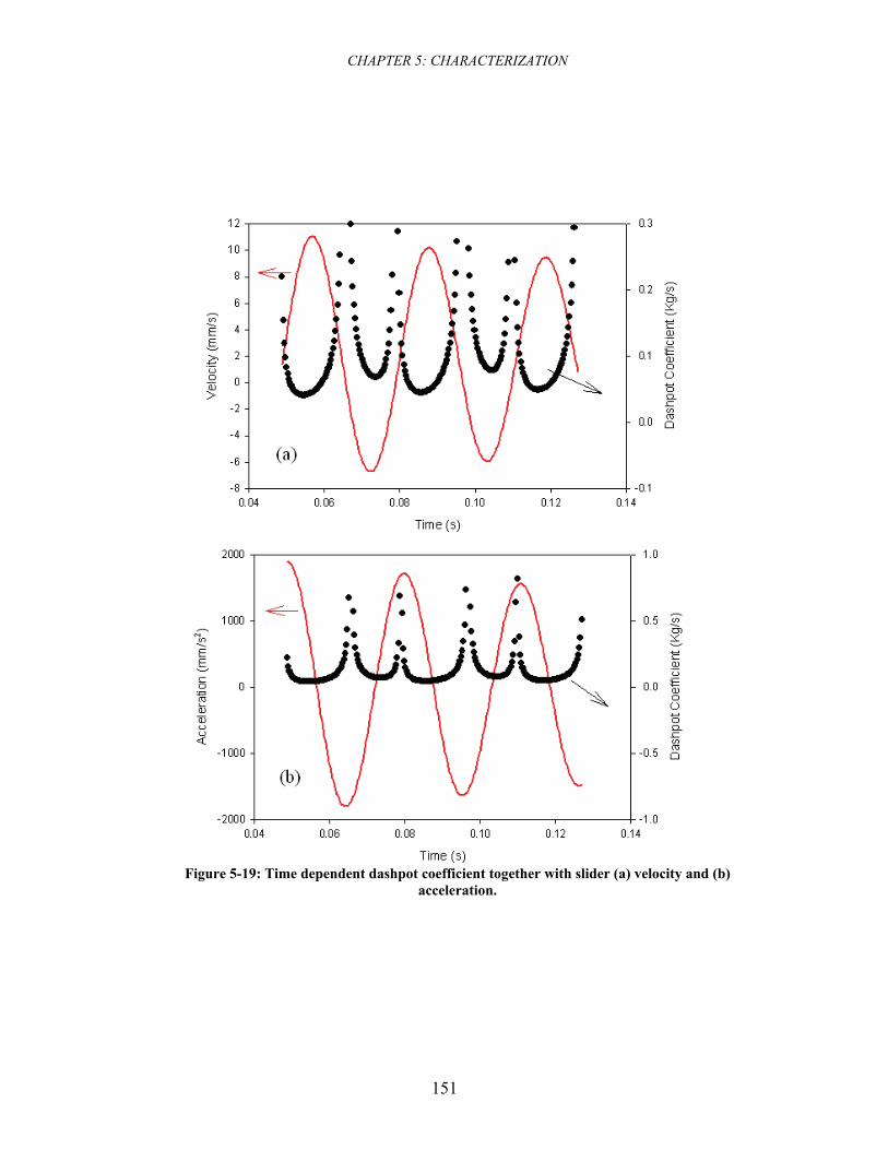
CHAPTER 5: CHARACTERIZATION
151
Figure 5-19: Time dependent dashpot coefficient together with slider (a) velocity and (b)
acceleration.
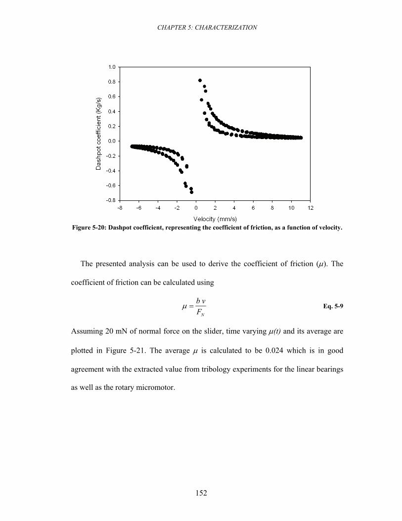
CHAPTER 5: CHARACTERIZATION
152
Figure 5-20: Dashpot coefficient, representing the coefficient of friction, as a function of velocity.
The presented analysis can be used to derive the coefficient of friction (μ). The
coefficient of friction can be calculated using
NFvb
=μ Eq. 5-9
Assuming 20 mN of normal force on the slider, time varying μ(t) and its average are
plotted in Figure 5-21. The average μ is calculated to be 0.024 which is in good
agreement with the extracted value from tribology experiments for the linear bearings
as well as the rotary micromotor.
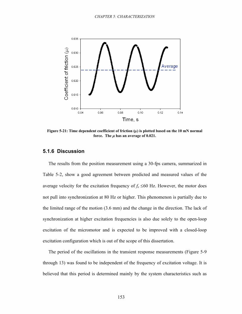
CHAPTER 5: CHARACTERIZATION
153
Figure 5-21: Time dependent coefficient of friction (μ) is plotted based on the 10 mN normal force. The μ has an average of 0.021.
5.1.6 Discussion
The results from the position measurement using a 30-fps camera, summarized in
Table 5-2, show a good agreement between predicted and measured values of the
average velocity for the excitation frequency of fe ≤60 Hz. However, the motor does
not pull into synchronization at 80 Hz or higher. This phenomenon is partially due to
the limited range of the motion (3.6 mm) and the change in the direction. The lack of
synchronization at higher excitation frequencies is also due solely to the open-loop
excitation of the micromotor and is expected to be improved with a closed-loop
excitation configuration which is out of the scope of this dissertation.
The period of the oscillations in the transient response measurements (Figure 5-9
through 13) was found to be independent of the frequency of excitation voltage. It is
believed that this period is determined mainly by the system characteristics such as
CHAPTER 5: CHARACTERIZATION
154
slider mass, friction, and electrostatic spring constant of a variable-capacitance
structure. The mass-dashpot-spring system presented earlier explains this behavior.
The mass of the slider was calculated from the volume of the slider and density of
silicon to be 0.1 gram. The measured net force, shown in Figure 5-13 and Figure
5-14, is the result of the electrostatic force produced by the micromachine and the
frictional force between microball bearings and the silicon housing. This force was
verified to be proportional to the square of voltage. It can be seen that the measured
net force (Figure 5-13) is less than the average aligning force obtained from
simulation (Figure 5-17). The friction force is calculated from the difference between
measured and simulated forces. The friction force is a function of the normal force on
the slider and, therefore, changes with slider position. Assuming a constant normal
force of 20 mN the coefficient of friction is calculated to be on average 0.02.
The presented mass-spring-dashpot model is a valuable tool to understand the
dynamics of the micromotor including electrostatic and frictional behavior. The
increase in the dashpot coefficient (b) with increase in the excitation voltage is due to
the increase in the normal force. As mentioned earlier, b is a coefficient which
represents the frictional force on the slider. This force is proportional to the normal
force on the slider and is increased with the increase in the applied voltage. Another
extracted parameter is the electrostatic spring constant (ks). For simplicity, ks was
chosen to be independent of the slider position (x). Furthermore, the spring constant
value, which increases with the increase in the applied voltage, is also a function of
device capacitance and slider position. The mass-dashpot-spring model was proven to
be a simple and suitable tool for extracting device parameters. Non-linear effects,
CHAPTER 5: CHARACTERIZATION
155
such as position dependency of the electrostatic spring, velocity dependency of the
friction force, and the microscale tribological effects (adhesion and hysteresis) were
considered to be negligible. The modeling results show that the micromotor is well
represented with a second-order linear system.
5.1.7 Summary
The fabrication and dynamic characterization of a 6-phase, bottom-drive, linear,
variable-capacitance micromotor (B-LVCM) supported on microball bearings was
reported in this section. The second-generation device is a 6-phase machine; whereas,
the first-generation device was tested in a 3-phase configuration. The improvements
in the fabrication process were the main reasons for this achievement. The second-
generation device showed more reliable and smoother motion. Top velocity of 7.2
mm/s was measured compared to 3.5 mm/s for the first generation device.
The slider position of the B-LVCM was measured using low- and high-speed
video cameras; the instantaneous and average velocity, acceleration, and net force
were extracted from the position measurement. Considering the effect of frictional
force in the operation of the micromotor, the measured force (0.2 mN peak) is in good
agreement with the simulated force (0.53 mN peak). The transient response of the
micromotor to square-pulse excitation was analyzed.
The B-LVCM was modeled with a mass-spring-dashpot system; the dashpot
coefficient and electrostatic spring constant were extracted from measurement results
at two different actuation voltages. The evaluation of these two values (b and ks), for
different micromotors with distinct electrical or mechanical designs, enables us to
determine the optimum design for a given application. The characterization
CHAPTER 5: CHARACTERIZATION
156
methodology presented in this chapter is applicable to a wide range of micromachines
and provides useful information for design, control, and understanding the dynamic
behavior of micromachines.
5.2 Rotary Micromotor Characterization
The fabrication of the micromotor was reported in Chapter 4. The output variables
determining the performance of the micromotor were discussed in chapters 2 and 3.
In this chapter the angular displacement, velocity, acceleration, torque, power, and
frictional losses of the fabricated devices are measured through non-contact
techniques. The test setup developed for the characterization of the micromotors is
discussed first. The non-contact steady-state and transient response measurement
methodology is discussed second. The results obtained after testing different designs
together with comparison between measured and theoretical values are reported at the
end of this chapter.
5.2.1 Test Setup
The characterization of the micromotor requires development of a test setup that is
capable of 6-phase voltage excitation and angular displacement measurement. The
block diagram of the setup is shown in Figure 5-22. The micromotor is excited with a
6-channel high-voltage pulse generator (shown in yellow). A LabVIEW interface and
a personal computer are used to program a data acquisition card (DAQ). The DAQ
card (model PCI-6722 from National Instruments) provides 6 analog output channels
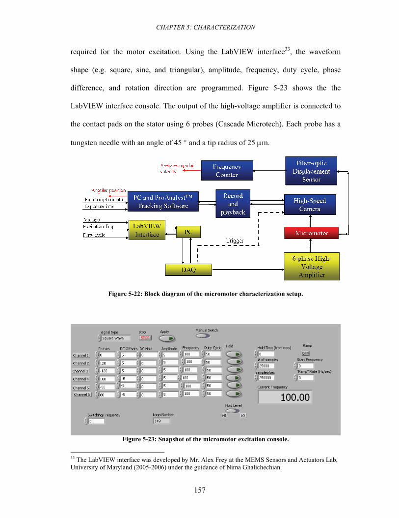
CHAPTER 5: CHARACTERIZATION
157
required for the motor excitation. Using the LabVIEW interface33, the waveform
shape (e.g. square, sine, and triangular), amplitude, frequency, duty cycle, phase
difference, and rotation direction are programmed. Figure 5-23 shows the the
LabVIEW interface console. The output of the high-voltage amplifier is connected to
the contact pads on the stator using 6 probes (Cascade Microtech). Each probe has a
tungsten needle with an angle of 45 ° and a tip radius of 25 μm.
Figure 5-22: Block diagram of the micromotor characterization setup.
Figure 5-23: Snapshot of the micromotor excitation console.
33 The LabVIEW interface was developed by Mr. Alex Frey at the MEMS Sensors and Actuators Lab, University of Maryland (2005-2006) under the guidance of Nima Ghalichechian.
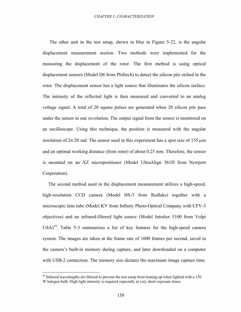
CHAPTER 5: CHARACTERIZATION
158
The other unit in the test setup, shown in blue in Figure 5-22, is the angular
displacement measurement section. Two methods were implemented for the
measuring the displacement of the rotor. The first method is using optical
displacement sensors (Model D6 from Philtech) to detect the silicon pits etched in the
rotor. The displacement sensor has a light source that illuminates the silicon surface.
The intensity of the reflected light is then measured and converted to an analog
voltage signal. A total of 20 square pulses are generated when 20 silicon pits pass
under the sensor in one revolution. The output signal from the sensor is monitored on
an oscilloscope. Using this technique, the position is measured with the angular
resolution of 2π/20 rad. The sensor used in this experiment has a spot size of 155 μm
and an optimal working distance (from rotor) of about 0.25 mm. Therefore, the sensor
is mounted on an XZ micropositioner (Model UltraAlign 561D from Newport
Corporation).
The second method used in the displacement measurement utilizes a high-speed,
high-resolution CCD camera (Model HS-3 from Redlake) together with a
microscopic lens tube (Model KV from Infinity Photo-Optical Company with CFV-3
objectives) and an infrared-filtered light source (Model Intralux 5100 from Volpi
USA)34. Table 5-3 summarizes a list of key features for the high-speed camera
system. The images are taken at the frame rate of 1000 frames per second, saved in
the camera’s built-in memory during capture, and later downloaded on a computer
with USB-2 connection. The memory size dictates the maximum image capture time.
34 Infrared wavelengths are filtered to prevent the test setup from heating up when lighted with a 150 W halogen bulb. High light intensity is required especially at very short exposure times.
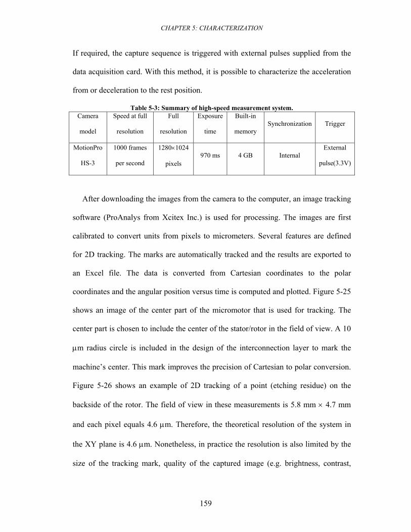
CHAPTER 5: CHARACTERIZATION
159
If required, the capture sequence is triggered with external pulses supplied from the
data acquisition card. With this method, it is possible to characterize the acceleration
from or deceleration to the rest position.
Table 5-3: Summary of high-speed measurement system. Camera
model
Speed at full
resolution
Full
resolution
Exposure
time
Built-in
memory Synchronization Trigger
MotionPro
HS-3
1000 frames
per second
1280×1024
pixels 970 ms 4 GB Internal
External
pulse(3.3V)
After downloading the images from the camera to the computer, an image tracking
software (ProAnalys from Xcitex Inc.) is used for processing. The images are first
calibrated to convert units from pixels to micrometers. Several features are defined
for 2D tracking. The marks are automatically tracked and the results are exported to
an Excel file. The data is converted from Cartesian coordinates to the polar
coordinates and the angular position versus time is computed and plotted. Figure 5-25
shows an image of the center part of the micromotor that is used for tracking. The
center part is chosen to include the center of the stator/rotor in the field of view. A 10
μm radius circle is included in the design of the interconnection layer to mark the
machine’s center. This mark improves the precision of Cartesian to polar conversion.
Figure 5-26 shows an example of 2D tracking of a point (etching residue) on the
backside of the rotor. The field of view in these measurements is 5.8 mm × 4.7 mm
and each pixel equals 4.6 μm. Therefore, the theoretical resolution of the system in
the XY plane is 4.6 μm. Nonetheless, in practice the resolution is also limited by the
size of the tracking mark, quality of the captured image (e.g. brightness, contrast,
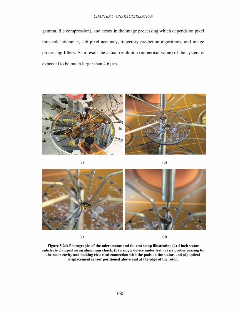
CHAPTER 5: CHARACTERIZATION
160
gamma, file compression), and errors in the image processing which depends on pixel
threshold tolerance, sub pixel accuracy, trajectory prediction algorithms, and image
processing filters. As a result the actual resolution (numerical value) of the system is
expected to be much larger than 4.6 μm.
(a) (b)
(c) (d)
Figure 5-24: Photographs of the micromotor and the test setup illustrating (a) 4 inch stator substrate clamped on an aluminum chuck, (b) a single device under test, (c) six probes passing by
the rotor cavity and making electrical connection with the pads on the stator, and (d) optical displacement sensor positioned above and at the edge of the rotor.
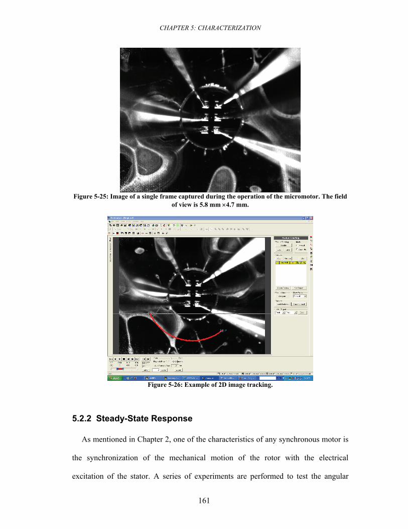
CHAPTER 5: CHARACTERIZATION
161
Figure 5-25: Image of a single frame captured during the operation of the micromotor. The field
of view is 5.8 mm ×4.7 mm.
Figure 5-26: Example of 2D image tracking.
5.2.2 Steady-State Response
As mentioned in Chapter 2, one of the characteristics of any synchronous motor is
the synchronization of the mechanical motion of the rotor with the electrical
excitation of the stator. A series of experiments are performed to test the angular
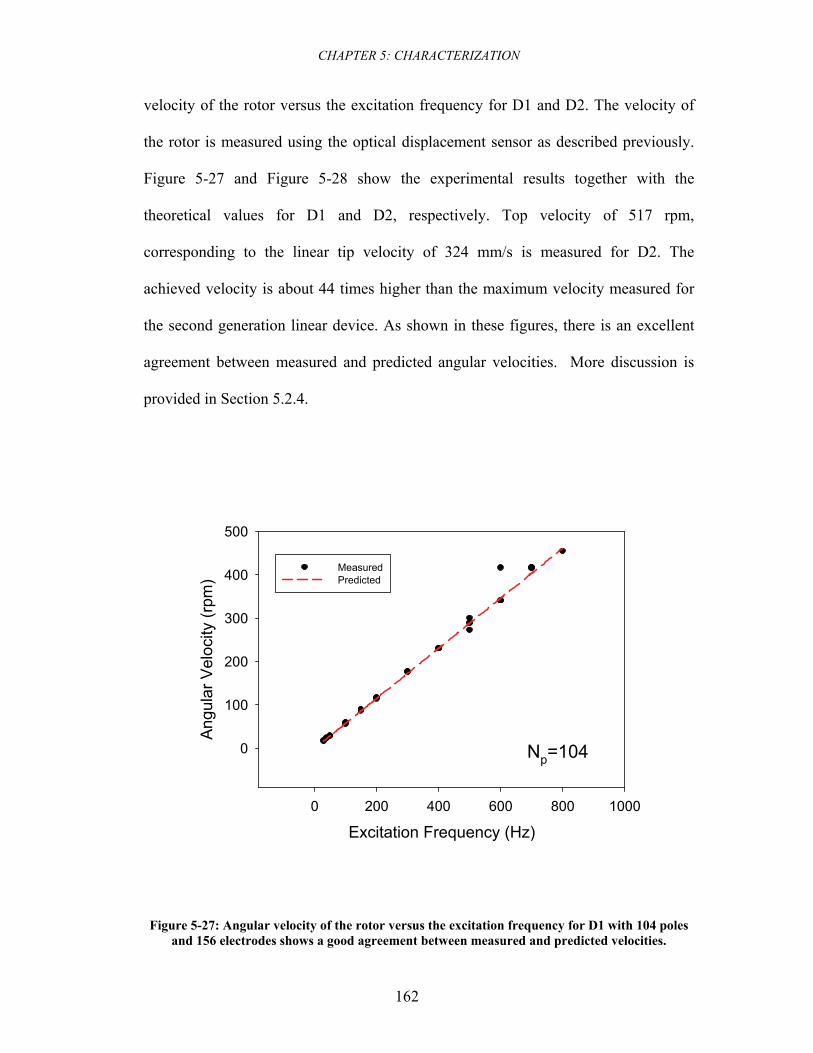
CHAPTER 5: CHARACTERIZATION
162
velocity of the rotor versus the excitation frequency for D1 and D2. The velocity of
the rotor is measured using the optical displacement sensor as described previously.
Figure 5-27 and Figure 5-28 show the experimental results together with the
theoretical values for D1 and D2, respectively. Top velocity of 517 rpm,
corresponding to the linear tip velocity of 324 mm/s is measured for D2. The
achieved velocity is about 44 times higher than the maximum velocity measured for
the second generation linear device. As shown in these figures, there is an excellent
agreement between measured and predicted angular velocities. More discussion is
provided in Section 5.2.4.
Excitation Frequency (Hz)0 200 400 600 800 1000
Ang
ular
Vel
ocity
(rpm
)
0
100
200
300
400
500
MeasuredPredicted
Np=104
Figure 5-27: Angular velocity of the rotor versus the excitation frequency for D1 with 104 poles
and 156 electrodes shows a good agreement between measured and predicted velocities.
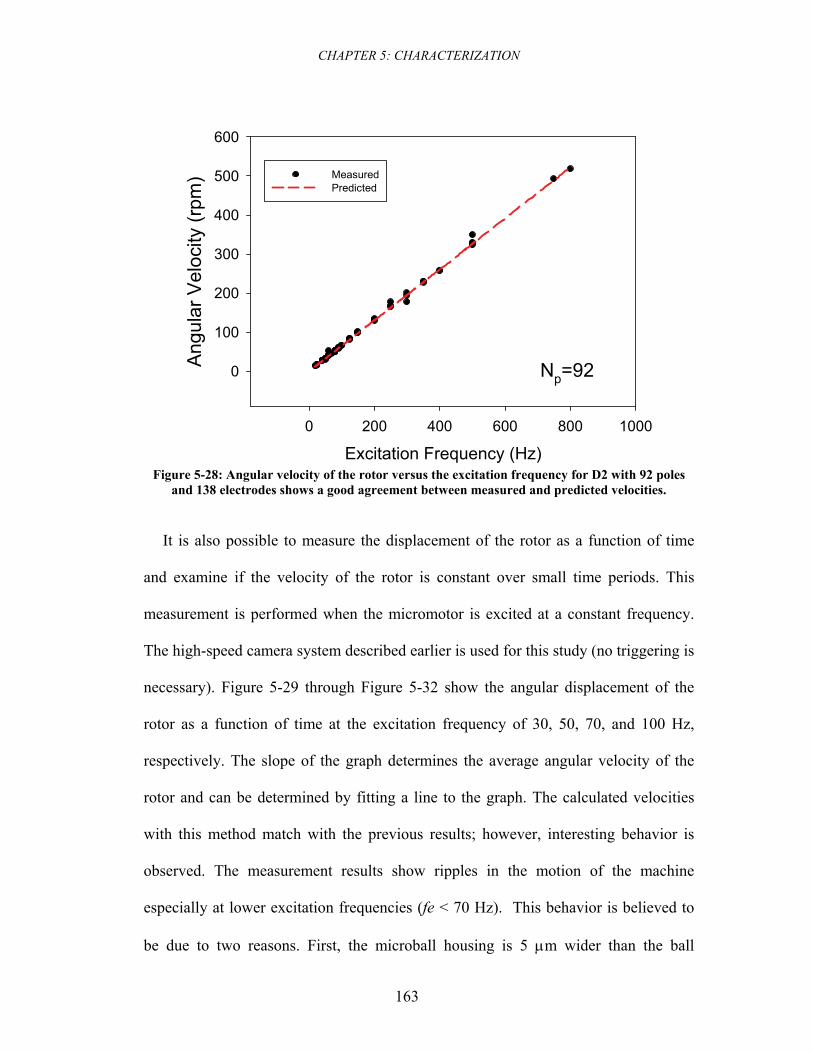
CHAPTER 5: CHARACTERIZATION
163
Excitation Frequency (Hz)0 200 400 600 800 1000
Ang
ular
Vel
ocity
(rpm
)
0
100
200
300
400
500
600
MeasuredPredicted
Np=92
Figure 5-28: Angular velocity of the rotor versus the excitation frequency for D2 with 92 poles
and 138 electrodes shows a good agreement between measured and predicted velocities.
It is also possible to measure the displacement of the rotor as a function of time
and examine if the velocity of the rotor is constant over small time periods. This
measurement is performed when the micromotor is excited at a constant frequency.
The high-speed camera system described earlier is used for this study (no triggering is
necessary). Figure 5-29 through Figure 5-32 show the angular displacement of the
rotor as a function of time at the excitation frequency of 30, 50, 70, and 100 Hz,
respectively. The slope of the graph determines the average angular velocity of the
rotor and can be determined by fitting a line to the graph. The calculated velocities
with this method match with the previous results; however, interesting behavior is
observed. The measurement results show ripples in the motion of the machine
especially at lower excitation frequencies (fe < 70 Hz). This behavior is believed to
be due to two reasons. First, the microball housing is 5 μm wider than the ball
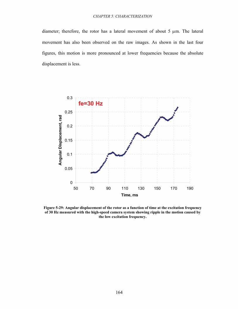
CHAPTER 5: CHARACTERIZATION
164
diameter; therefore, the rotor has a lateral movement of about 5 μm. The lateral
movement has also been observed on the raw images. As shown in the last four
figures, this motion is more pronounced at lower frequencies because the absolute
displacement is less.
fe=30 Hz
0
0.05
0.1
0.15
0.2
0.25
0.3
50 70 90 110 130 150 170 190Time, ms
Ang
ular
Dis
plac
emen
t, ra
d
Figure 5-29: Angular displacement of the rotor as a function of time at the excitation frequency of 30 Hz measured with the high-speed camera system showing ripple in the motion caused by
the low excitation frequency.
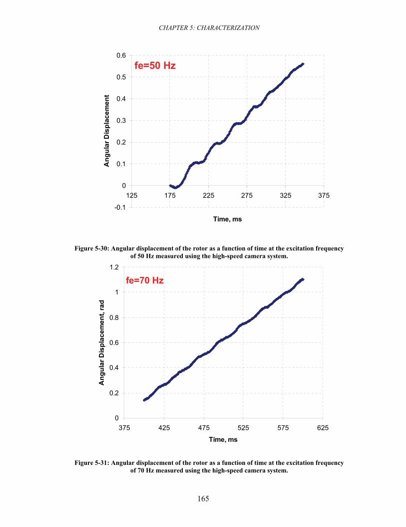
CHAPTER 5: CHARACTERIZATION
165
fe=50 Hz
-0.1
0
0.1
0.2
0.3
0.4
0.5
0.6
125 175 225 275 325 375
Time, ms
Ang
ular
Dis
plac
emen
t
Figure 5-30: Angular displacement of the rotor as a function of time at the excitation frequency of 50 Hz measured using the high-speed camera system.
fe=70 Hz
0
0.2
0.4
0.6
0.8
1
1.2
375 425 475 525 575 625
Time, ms
Ang
ular
Dis
plac
emen
t, ra
d
Figure 5-31: Angular displacement of the rotor as a function of time at the excitation frequency of 70 Hz measured using the high-speed camera system.
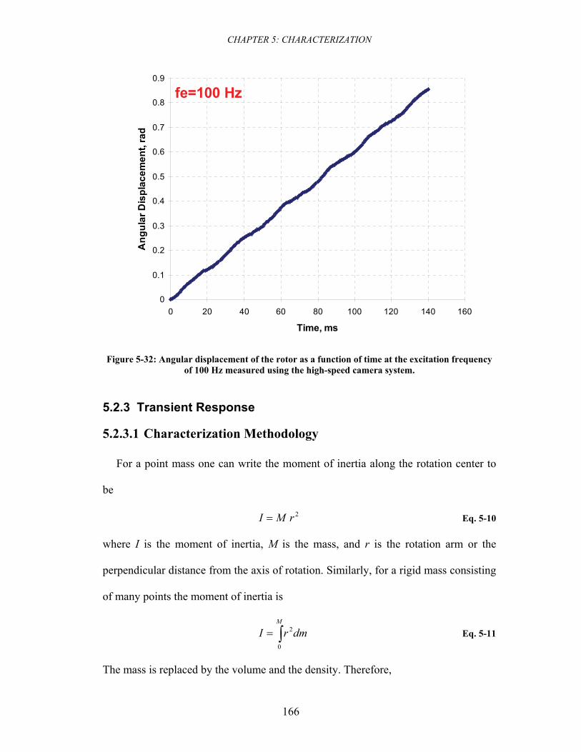
CHAPTER 5: CHARACTERIZATION
166
fe=100 Hz
0
0.1
0.2
0.3
0.4
0.5
0.6
0.7
0.8
0.9
0 20 40 60 80 100 120 140 160
Time, ms
Ang
ular
Dis
plac
emen
t, ra
d
Figure 5-32: Angular displacement of the rotor as a function of time at the excitation frequency of 100 Hz measured using the high-speed camera system.
5.2.3 Transient Response
5.2.3.1 Characterization Methodology
For a point mass one can write the moment of inertia along the rotation center to
be
2rMI = Eq. 5-10
where I is the moment of inertia, M is the mass, and r is the rotation arm or the
perpendicular distance from the axis of rotation. Similarly, for a rigid mass consisting
of many points the moment of inertia is
∫=M
dmrI0
2 Eq. 5-11
The mass is replaced by the volume and the density. Therefore,
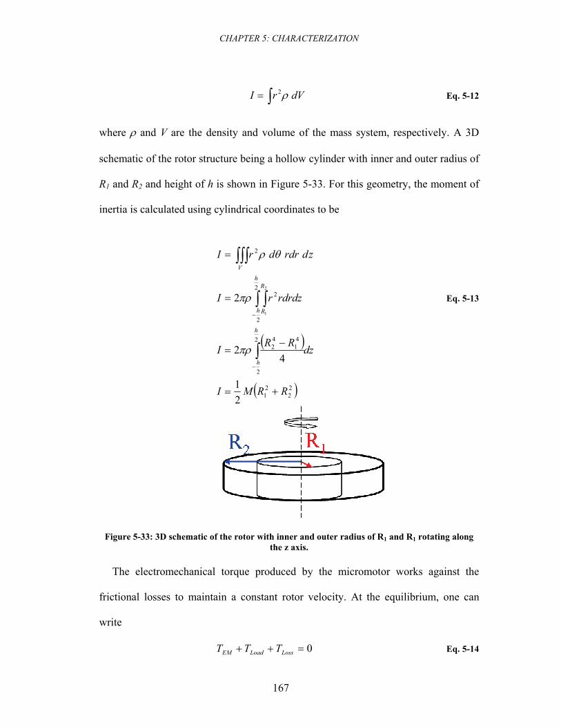
CHAPTER 5: CHARACTERIZATION
167
∫= dVrI ρ2 Eq. 5-12
where ρ and V are the density and volume of the mass system, respectively. A 3D
schematic of the rotor structure being a hollow cylinder with inner and outer radius of
R1 and R2 and height of h is shown in Figure 5-33. For this geometry, the moment of
inertia is calculated using cylindrical coordinates to be
( )
( )22
21
2
2
41
42
2
2
2
2
21
42
22
1
RRMI
dzRR
I
rdrdzrI
zdrdrdrI
h
h
h
h
R
R
V
+=
−=
=
=
∫
∫ ∫
∫∫∫
−
−
πρ
πρ
θρ
Eq. 5-13
Figure 5-33: 3D schematic of the rotor with inner and outer radius of R1 and R1 rotating along the z axis.
The electromechanical torque produced by the micromotor works against the
frictional losses to maintain a constant rotor velocity. At the equilibrium, one can
write
0=++ LossLoadEM TTT Eq. 5-14
CHAPTER 5: CHARACTERIZATION
168
where TEM is the electromechanical torque of the machine, TLoss is the loss torque
composed of frictional, viscous drag and other losses, and TLoad is the load torque
which is the result of moment of inertia of the rotor and angular acceleration. TLoad at
any time can be written as
ITLoad α= Eq. 5-15
where α and I are the angular acceleration and moment of inertia of the rotor,
respectively. One of the characteristics of a variable-capacitance machine is that the
velocity of the rotor is proportional to the excitation frequency and stays constant for
a fixed frequency. At the constant velocity regime
0==dtdωα Eq. 5-16
Therefore the TLoad term is zero and we can write
0=+ LossEM TT Eq. 5-17
By measuring TLoss the electromechanical torque of the machine can be calculated to
be
LossEM TT −= Eq. 5-18
TLoss can be extracted from transient analysis measurement. In this method, the motor
is spun at a constant velocity, then at t=0 the applied voltage to all 6 phases is set to
V=0 V. Therefore,
00 ==VEMT Eq. 5-19
The main torque equation can now be written as
0=+ LossLoad TT Eq. 5-20
ITT LoadLoss α−=−= Eq. 5-21
CHAPTER 5: CHARACTERIZATION
169
Therefore, by measuring the rotor deceleration (α) at t>0 the loss torque with no
applied voltage can be calculated. Assuming that the frictional losses are the
dominant loss mechanism for a micromotor rotating at relatively low speeds, the
frictional torque is
ITT LossFriction α−== Eq. 5-22
The frictional force can be modeled at the product of the normal force and the
coefficient of friction. Therefore,
0RMgTFriction ××= μ Eq. 5-23
where μ is the coefficient of friction (COF), Mg is the weight of the rotor, and R0 is
the radius of the bearing. The coefficient of friction can be calculated from
( )α
ααμ43421
.
0
22
21
0
22
21
00 221
Const
Friction
gRRR
MgR
RRM
MgRI
MgRT +
=+
=== Eq. 5-24
After the rotor deceleration is measured, the COF is extracted from above equation.
The electromechanical torque of the machine at V=V0 can also be extracted from
the same measurement. Assuming that the COF is not a function of the normal force
(FN), the electromechanical torque is equal to the frictional torque at a constant
velocity.
RFT NVVEM ××== μ0
Eq. 5-25
( )( ) α44 344 21
.
22
210
20
const
NVVEM g
RRVFT +== Eq. 5-26
The above equation is used for the torque extraction after the measurement of
deceleration. Experiments have shown that the machine does not operate at excitation
CHAPTER 5: CHARACTERIZATION
170
amplitudes lower than 150V. The change in the power angle of the machine to
balance the load and electromechanical torque was discussed in Chapter 2. If the
applied voltage, V0, is the onset of operation i.e. the spinning motor would stop if
lower voltage is applied, the power angle of the machine is at the critical value35. The
FN(V0) value is obtained from the 3D finite element simulations reported in Chapter 3.
5.2.3.2 Angular Velocity and Acceleration
It was described in Section 5.2.3.1 that the transient response of the micromotor is
used to extract the electromechanical torque, frictional torque, and coefficient of
friction. In this type of measurement, the micromotor is excited with square pulses
with constant amplitude, frequency, and duty cycle. At t=0 s, the applied voltage is
set to be zero; however, the rotor does not stop immediately since it has a finite
angular momentum of Iω. Because the motion detection system has a high temporal
resolution (1 ms) and is triggered at t=0 s, it is possible to measure the angular
displacement of the rotor with high precision at the time period of t<0 and t=ts where
ts is the time when rotor completely stops.
The angular velocity, ω(t), and angular acceleration, α(t), can be obtained by
taking the first and second numerical derivative of position (θ(t)). However,
numerical differentiation amplifies noise. Therefore, it is necessary to filter the
position data (e.g. smoothing) or fit the position data to a function. The current
methodology uses the curve fitting method. The first step is to find a function that fits
well to the data and has a rational correspondence with the physics of the problem. In
order to find an appropriate θ(t) function a differential equation of 35 For more information please refer to the power angle discussion in Chapter 2.
CHAPTER 5: CHARACTERIZATION
171
BA += θθ &&& Eq. 5-27
is defined to express the angular acceleration of the system as a linear function of the
angular velocity, where θ&& and θ& are the second and first derivatives of the angular
displacement with respect to time. The above equation is written based on the
assumption that the coefficient of friction is constant plus some linear dependence on
the angular velocity. This approach allows velocity dependant COF and is justified
after comparison to the measured data. One solution of such differential equation is36
dctaebt ++=θ Eq. 5-28
where A = b and B = − bc. The first and second derivatives of the displacement are
respectively
cabebt +=θ& Eq. 5-29
bteab2=θ&& Eq. 5-30
Figure 5-34 shows the angular displacement of the rotor together with the fitted
curve with R2 value of 0.9999. The fitting is performed using the MATLAB Curve
Fitting Toolbox. After the curve fit a, b, c, and d constants are obtained with 95%
confidence bound. A good agreement between assumed model and measured data is
shown in the figure. Table 5-4 lists the summary of the fitting parameters. θ&& and θ&
are then calculated using the constants and the last two equations. The angular
position, velocity and acceleration results for 0<t<1 s are shown in Figure 5-35,
Figure 5-36, and Figure 5-37, respectively. The excitation frequency of 300 Hz
corresponds to the initial rotor velocity of 20.5 rad/s. From Figure 5-36, the initial
36 Final solution is only reported.
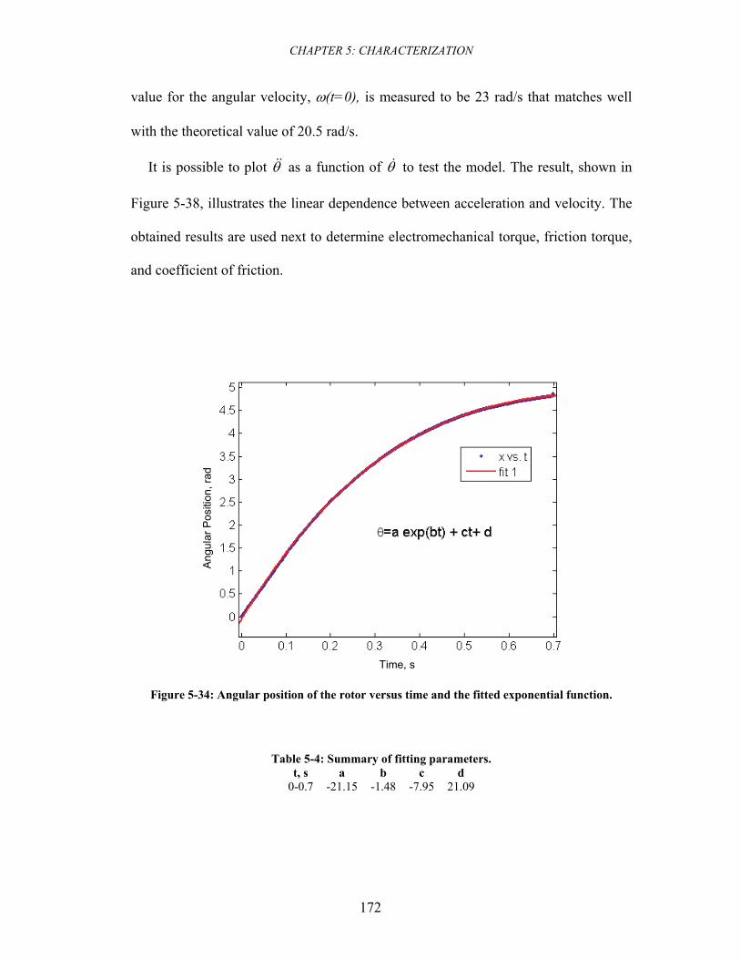
CHAPTER 5: CHARACTERIZATION
172
value for the angular velocity, ω(t=0), is measured to be 23 rad/s that matches well
with the theoretical value of 20.5 rad/s.
It is possible to plot θ&& as a function of θ& to test the model. The result, shown in
Figure 5-38, illustrates the linear dependence between acceleration and velocity. The
obtained results are used next to determine electromechanical torque, friction torque,
and coefficient of friction.
Figure 5-34: Angular position of the rotor versus time and the fitted exponential function.
Table 5-4: Summary of fitting parameters. t, s a b c d
0-0.7 -21.15 -1.48 -7.95 21.09
Time, s
Ang
ular
Pos
ition
, rad
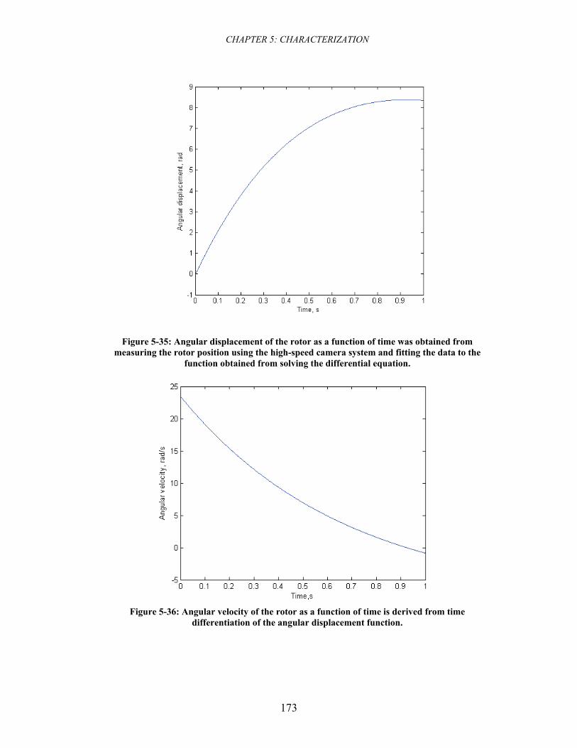
CHAPTER 5: CHARACTERIZATION
173
Figure 5-35: Angular displacement of the rotor as a function of time was obtained from measuring the rotor position using the high-speed camera system and fitting the data to the
function obtained from solving the differential equation.
Figure 5-36: Angular velocity of the rotor as a function of time is derived from time
differentiation of the angular displacement function.
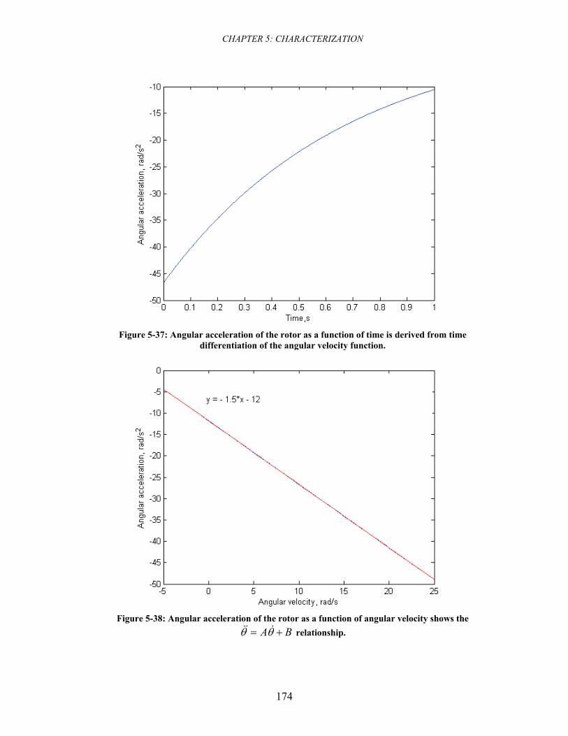
CHAPTER 5: CHARACTERIZATION
174
Figure 5-37: Angular acceleration of the rotor as a function of time is derived from time
differentiation of the angular velocity function.
Figure 5-38: Angular acceleration of the rotor as a function of angular velocity shows the
BA += θθ &&& relationship.
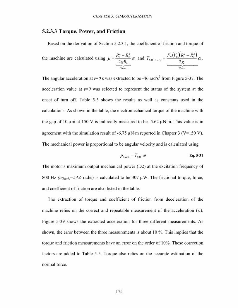
CHAPTER 5: CHARACTERIZATION
175
5.2.3.3 Torque, Power, and Friction
Based on the derivation of Section 5.2.3.1, the coefficient of friction and torque of
the machine are calculated using αμ43421
.
0
22
21
2Const
gRRR +
= and ( )( ) α44 344 21
.
22
210
20
Const
NVVEM g
RRVFT +== .
The angular acceleration at t=0 s was extracted to be -46 rad/s2 from Figure 5-37. The
acceleration value at t=0 was selected to represent the status of the system at the
onset of turn off. Table 5-5 shows the results as well as constants used in the
calculations. As shown in the table, the electromechanical torque of the machine with
the gap of 10 μm at 150 V is indirectly measured to be -5.62 μN⋅m. This value is in
agreement with the simulation result of -6.75 μN⋅m reported in Chapter 3 (V=150 V).
The mechanical power is proportional to be angular velocity and is calculated using
ωEMMech Tp =. Eq. 5-31
The motor’s maximum output mechanical power (D2) at the excitation frequency of
800 Hz (ωMech.=54.6 rad/s) is calculated to be 307 μW. The frictional torque, force,
and coefficient of friction are also listed in the table.
The extraction of torque and coefficient of friction from deceleration of the
machine relies on the correct and repeatable measurement of the acceleration (α).
Figure 5-39 shows the extracted acceleration for three different measurements. As
shown, the error between the three measurements is about 10 %. This implies that the
torque and friction measurements have an error on the order of 10%. These correction
factors are added to Table 5-5. Torque also relies on the accurate estimation of the
normal force.
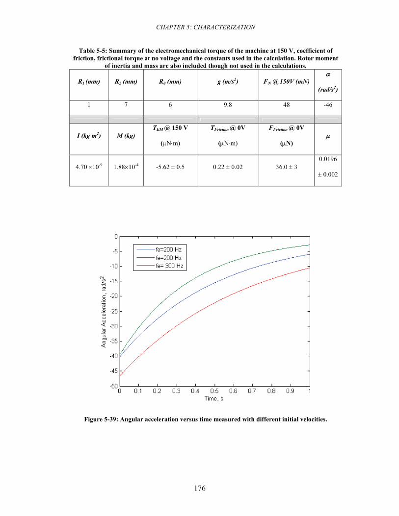
CHAPTER 5: CHARACTERIZATION
176
Table 5-5: Summary of the electromechanical torque of the machine at 150 V, coefficient of friction, frictional torque at no voltage and the constants used in the calculation. Rotor moment
of inertia and mass are also included though not used in the calculations.
R1 (mm) R2 (mm) R0 (mm) g (m/s2) FN @ 150V (mN) α
(rad/s2)
1 7 6 9.8 48 -46
I (kg m2) M (kg) TEM @ 150 V
(μN⋅m)
TFriction @ 0V
(μN⋅m)
FFriction @ 0V
(μN) μ
4.70 ×10⁻⁹ 1.88×10⁻⁴ -5.62 ± 0.5 0.22 ± 0.02 36.0 ± 3 0.0196
± 0.002
Figure 5-39: Angular acceleration versus time measured with different initial velocities.
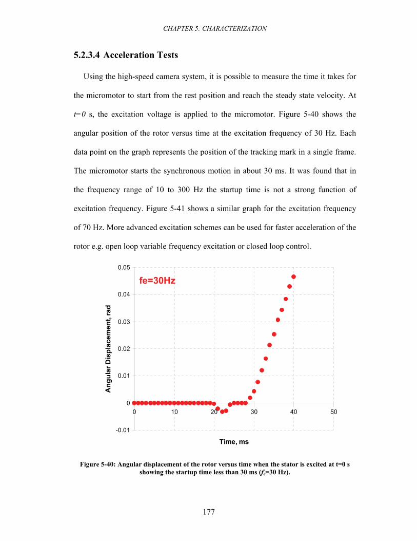
CHAPTER 5: CHARACTERIZATION
177
5.2.3.4 Acceleration Tests
Using the high-speed camera system, it is possible to measure the time it takes for
the micromotor to start from the rest position and reach the steady state velocity. At
t=0 s, the excitation voltage is applied to the micromotor. Figure 5-40 shows the
angular position of the rotor versus time at the excitation frequency of 30 Hz. Each
data point on the graph represents the position of the tracking mark in a single frame.
The micromotor starts the synchronous motion in about 30 ms. It was found that in
the frequency range of 10 to 300 Hz the startup time is not a strong function of
excitation frequency. Figure 5-41 shows a similar graph for the excitation frequency
of 70 Hz. More advanced excitation schemes can be used for faster acceleration of the
rotor e.g. open loop variable frequency excitation or closed loop control.
fe=30Hz
-0.01
0
0.01
0.02
0.03
0.04
0.05
0 10 20 30 40 50
Time, ms
Ang
ular
Dis
plac
emen
t, ra
d
Figure 5-40: Angular displacement of the rotor versus time when the stator is excited at t=0 s showing the startup time less than 30 ms (fe=30 Hz).
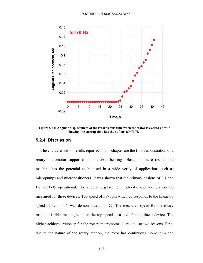
CHAPTER 5: CHARACTERIZATION
178
fe=70 Hz
-0.02
0
0.02
0.04
0.06
0.08
0.1
0.12
0.14
0.16
0 5 10 15 20 25 30 35 40 45
Time, s
Ang
ular
Dis
plac
emen
t, ra
d
Figure 5-41: Angular displacement of the rotor versus time when the stator is excited at t=0 s showing the startup time less than 30 ms (fe=70 Hz).
5.2.4 Discussion
The characterization results reported in this chapter are the first demonstration of a
rotary micromotor supported on microball bearings. Based on these results, the
machine has the potential to be used in a wide verity of applications such as
micropumps and micropositioners. It was shown that the primary designs of D1 and
D2 are both operational. The angular displacement, velocity, and acceleration are
measured for these devices. Top speed of 517 rpm which corresponds to the linear tip
speed of 324 mm/s was demonstrated for D2. The measured speed for the rotary
machine is 44 times higher than the top speed measured for the linear device. The
higher achieved velocity for the rotary micromotor is credited to two reasons. First,
due to the nature of the rotary motion, the rotor has continuous momentum and
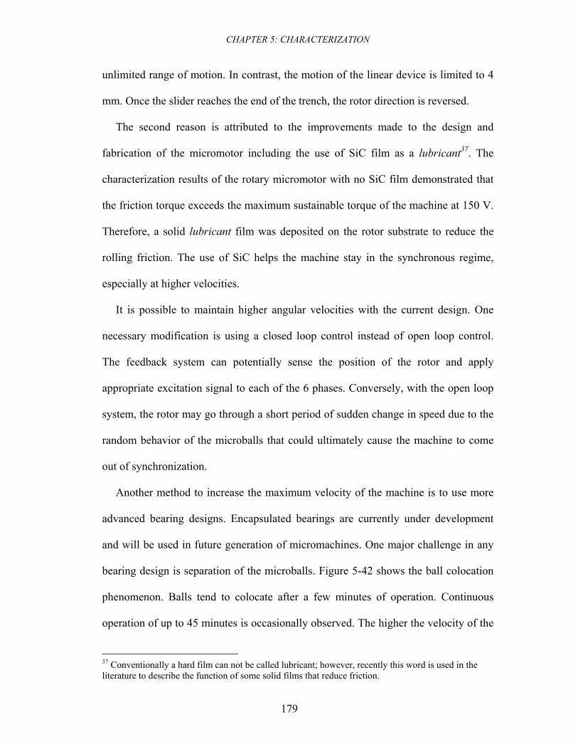
CHAPTER 5: CHARACTERIZATION
179
unlimited range of motion. In contrast, the motion of the linear device is limited to 4
mm. Once the slider reaches the end of the trench, the rotor direction is reversed.
The second reason is attributed to the improvements made to the design and
fabrication of the micromotor including the use of SiC film as a lubricant37. The
characterization results of the rotary micromotor with no SiC film demonstrated that
the friction torque exceeds the maximum sustainable torque of the machine at 150 V.
Therefore, a solid lubricant film was deposited on the rotor substrate to reduce the
rolling friction. The use of SiC helps the machine stay in the synchronous regime,
especially at higher velocities.
It is possible to maintain higher angular velocities with the current design. One
necessary modification is using a closed loop control instead of open loop control.
The feedback system can potentially sense the position of the rotor and apply
appropriate excitation signal to each of the 6 phases. Conversely, with the open loop
system, the rotor may go through a short period of sudden change in speed due to the
random behavior of the microballs that could ultimately cause the machine to come
out of synchronization.
Another method to increase the maximum velocity of the machine is to use more
advanced bearing designs. Encapsulated bearings are currently under development
and will be used in future generation of micromachines. One major challenge in any
bearing design is separation of the microballs. Figure 5-42 shows the ball colocation
phenomenon. Balls tend to colocate after a few minutes of operation. Continuous
operation of up to 45 minutes is occasionally observed. The higher the velocity of the
37 Conventionally a hard film can not be called lubricant; however, recently this word is used in the literature to describe the function of some solid films that reduce friction.
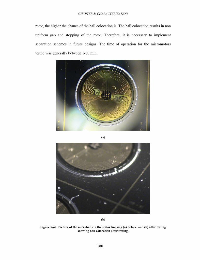
CHAPTER 5: CHARACTERIZATION
180
rotor, the higher the chance of the ball colocation is. The ball colocation results in non
uniform gap and stopping of the rotor. Therefore, it is necessary to implement
separation schemes in future designs. The time of operation for the micromotors
tested was generally between 1-60 min.
(a)
(b)
Figure 5-42: Picture of the microballs in the stator housing (a) before, and (b) after testing showing ball colocation after testing.
CHAPTER 5: CHARACTERIZATION
181
Other micromotor designs (D3-6) were also tested in a similar manner. It was
observed that the high-torque design (D4) is operational; however, the machine’s
operation is neither continuous nor reliable. D4 was originally designed for a 5 μm
gap size; however, such a small gap has not been achieved in this study. Further
improvements to the fabrication process are necessary to maintain a small uniform
gap. Unreliable operation of the machine is not necessarily due to the electrode
geometry design. The behavior can also be attributed to the high normal force
compared to D1 and D2 and therefore, higher friction torque.
Among the other designs, D3, D5, and D6 were never successfully tested. It is
believed that D3’s theoretical maximum torque is not sufficient to overcome the
friction for the current bearing design. D5 and D6 have both double-trench bearings
that are believed to result in higher friction or less stability due to the imperfections in
the fabrication process of the two trenches.
The measurement results of the machine’s angular velocity shows an excellent
agreement between theory and experiment (Figure 5-27 and Figure 5-28). It was
discussed in Chapter 2 that the angular velocity of these types of machines is
formulated by nr=60 fe / Np. Three methods for the derivation of velocity were
reported in Chapter 2 that all differ from the commonly used formulation in the
literature (nr=120 fe / Np). The theoretical derivation supported by the experimental
results show that direct adaptation of the magnetic machine’s equation for the
electrostatic machines results in overestimation of the angular velocity. If such
adaptations are pursued, the difference in the nature of the two should be taken into
consideration. The most important disparity is concealed in the definition of the poles.
CHAPTER 5: CHARACTERIZATION
182
In an electromagnetic machine, poles are defined by the stator circuitry. Each S-N
pair makes a single pole. For a variable-capacitance machine, however, the definition
of poles has to be altered because a capacitor is formed by two conductors, one
physically located on the stator and one on the rotor. Without the existence of the
capacitor, the operation of the machine is not possible. Therefore, the numbers of
stator and rotor saliencies are both taken into consideration. This subject was
discussed in Chapter 2. The experimental results reported in this chapter support the
developed theory for these types of machines. The theory and the experimental
results, contradicting the literature, are both presented for the first time in this
dissertation.
The electromechanical torque is indirectly measured for the excitation voltage of
±150 V to be -5.62 μN⋅m. This value is in agreement with the simulation result of -
6.75 μN⋅m. It is desirable to measure the torque at different excitation voltages;
however, with the current test setup the maximum applied voltage is limited to ±150
V. Micromotor operation below 150 V was not achieved. The maximum output
mechanical power was calculated to be 307 μW (at ±150 V).
One of the advantages of the developed characterization methodology is the ability
to extract frictional torque and COF from the measurements. The accuracy of the
calculated COF solely depends on the geometrical factors and the measured
acceleration. The COF was measured to be around 0.02 which corresponds to the
interaction between stainless steel microballs, silicon housing on the stator, and SiC-
coated silicon housing on the rotor. The loading and the number of the microballs are
also a factor. In all the experiments discussed in Section 5.2, 10 microballs are used;
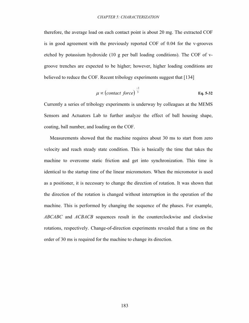
CHAPTER 5: CHARACTERIZATION
183
therefore, the average load on each contact point is about 20 mg. The extracted COF
is in good agreement with the previously reported COF of 0.04 for the v-grooves
etched by potassium hydroxide (10 g per ball loading conditions). The COF of v-
groove trenches are expected to be higher; however, higher loading conditions are
believed to reduce the COF. Recent tribology experiments suggest that [134]
( ) 31−
∝ forcecontactμ Eq. 5-32
Currently a series of tribology experiments is underway by colleagues at the MEMS
Sensors and Actuators Lab to further analyze the effect of ball housing shape,
coating, ball number, and loading on the COF.
Measurements showed that the machine requires about 30 ms to start from zero
velocity and reach steady state condition. This is basically the time that takes the
machine to overcome static friction and get into synchronization. This time is
identical to the startup time of the linear micromotors. When the micromotor is used
as a positioner, it is necessary to change the direction of rotation. It was shown that
the direction of the rotation is changed without interruption in the operation of the
machine. This is performed by changing the sequence of the phases. For example,
ABCABC and ACBACB sequences result in the counterclockwise and clockwise
rotations, respectively. Change-of-direction experiments revealed that a time on the
order of 30 ms is required for the machine to change its direction.
CHAPTER 6: SUMMARY AND CONCLUSION
184
6 Summary and Conclusion
6.1 Summary
The successful development of the first rotary micromotor supported on microball
bearings was demonstrated in this dissertation. The micromotor is a six-phase
variable-capacitance machine composed of stator, rotor, and microballs. Compared to
their magnetic counterparts, variable-capacitance machines are voltage driven, have a
comparable energy density at small gaps, and have a simpler fabrication process.
Furthermore, they are more efficient, have a lighter rotor, and can potentially be
operated at higher temperatures. Nevertheless, one of the major challenges in the
development of electric micromachines has been the robustness of the rotor
mechanical support. Previous designs utilize gas-lubricated bearings in
turbomachinery or center-pin bearings in early surface-micromachined devices. The
fabrication of the gas-lubricated bearings is extremely complex. The micromotors
based on center-pin bearings are highly inefficient and unreliable. The microball-
bearings technology in silicon provides a reliable support with less friction and wear
compared to center-pin bearings and less fabrication complexity compared to gas-
lubricated bearings. Another advantage is the ability to sustain uniform air gap, which
is critical for the operation of the micromachine. Furthermore, this technology
enables higher torques due to the implementation of a bottom-drive design.
The theory of the machine’s operation, including derivation of angular velocity
and torque, are fully discussed in Chapter 2. The machine’s geometry is designed
based on finite element simulation results. The effect of the electrodes packing factor
as well as the gap size on the torque of the machine was studied through a series of
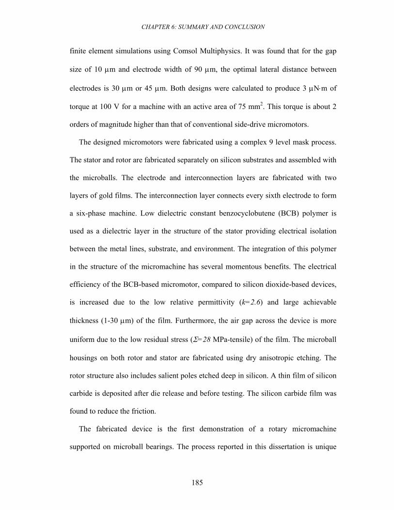
CHAPTER 6: SUMMARY AND CONCLUSION
185
finite element simulations using Comsol Multiphysics. It was found that for the gap
size of 10 μm and electrode width of 90 μm, the optimal lateral distance between
electrodes is 30 μm or 45 μm. Both designs were calculated to produce 3 μN⋅m of
torque at 100 V for a machine with an active area of 75 mm2. This torque is about 2
orders of magnitude higher than that of conventional side-drive micromotors.
The designed micromotors were fabricated using a complex 9 level mask process.
The stator and rotor are fabricated separately on silicon substrates and assembled with
the microballs. The electrode and interconnection layers are fabricated with two
layers of gold films. The interconnection layer connects every sixth electrode to form
a six-phase machine. Low dielectric constant benzocyclobutene (BCB) polymer is
used as a dielectric layer in the structure of the stator providing electrical isolation
between the metal lines, substrate, and environment. The integration of this polymer
in the structure of the micromachine has several momentous benefits. The electrical
efficiency of the BCB-based micromotor, compared to silicon dioxide-based devices,
is increased due to the low relative permittivity (k=2.6) and large achievable
thickness (1-30 μm) of the film. Furthermore, the air gap across the device is more
uniform due to the low residual stress (Σ=28 MPa-tensile) of the film. The microball
housings on both rotor and stator are fabricated using dry anisotropic etching. The
rotor structure also includes salient poles etched deep in silicon. A thin film of silicon
carbide is deposited after die release and before testing. The silicon carbide film was
found to reduce the friction.
The fabricated device is the first demonstration of a rotary micromachine
supported on microball bearings. The process reported in this dissertation is unique
CHAPTER 6: SUMMARY AND CONCLUSION
186
and extremely complicated; this work is the result of careful process development
carried out to address the adhesion of metal-polymer films, process yield, eccentricity
due to misalignment of electrodes to microball housing, interconnection resistance,
and small gap size. The rotary device significantly benefited from the process
characterization performed throughout the development of the second-generation
linear device, which by itself, was a major improvement to the first-generation.
The test setup originally developed for the characterization of the second-
generation linear micromotor was modified to accommodate the steady state and
transient response measurement. A top angular velocity of 517 rpm was measured
corresponding to a linear tip velocity of 324 mm/s; this is 44 times higher than the top
velocity measured for the linear device (7.2 mm/s). The electromechanical torque was
indirectly measured for the excitation voltage of ±150 V to be -5.62±0.5 μN⋅m. This
value is in agreement with the simulation result of -6.75 μN⋅m. The maximum output
mechanical power at ±150 V and 517 rpm was calculated to be 307 μW.
One of the benefits of the characterization methodology discussed in this
dissertation is the capability to extract COF from the transient measurements. The
COF was measured to be 0.02 which is in good agreement with our previous
tribology experiments and literature.
6.2 Contributions
Major contributions of this research dissertation are:
• Development of the first rotary micromotor supported on microball bearings
with top measured velocity of 517 rpm and torque of 5.6 μN⋅m.
CHAPTER 6: SUMMARY AND CONCLUSION
187
• Development of the second-generation linear micromotors supported on
microball bearings with top speed of 7.3 mm/s.
• Optimization of the fabrication process for linear machines.
• Dynamic characterization of the linear micromotors to indirectly obtain the
net slider force.
• Modeling of the linear micromotors and extraction of model parameters from
experiments.
• Feasibility demonstration of a microball bearing technology as a support
mechanism for rotary machines.
• Design and 3D finite element simulation of a rotary variable-capacitance
micromachine.
• Development of complex fabrication process using a 9-level-mask process.
• Integration of the benzocyclobutene polymer (as a low permittivity dielectric
material) with thin film deposition and silicon bulk micromachining.
• Implementation of a solid silicon carbide layer as a lubricant film.
• Development of a new characterization methodology for indirect
measurement of torque and coefficient of friction.
6.3 Future Work
The evolution of future microsystems that are capable of microsurgery,
micropropulsion, micropumping, and microassembly functions requires the
development of reliable, low-power, and efficient micromotors. Previous
micromotors suffer from friction, wear, stability, and fabrication complexities. A
major challenge in developing instrumental micromotors is to design and fabricate a
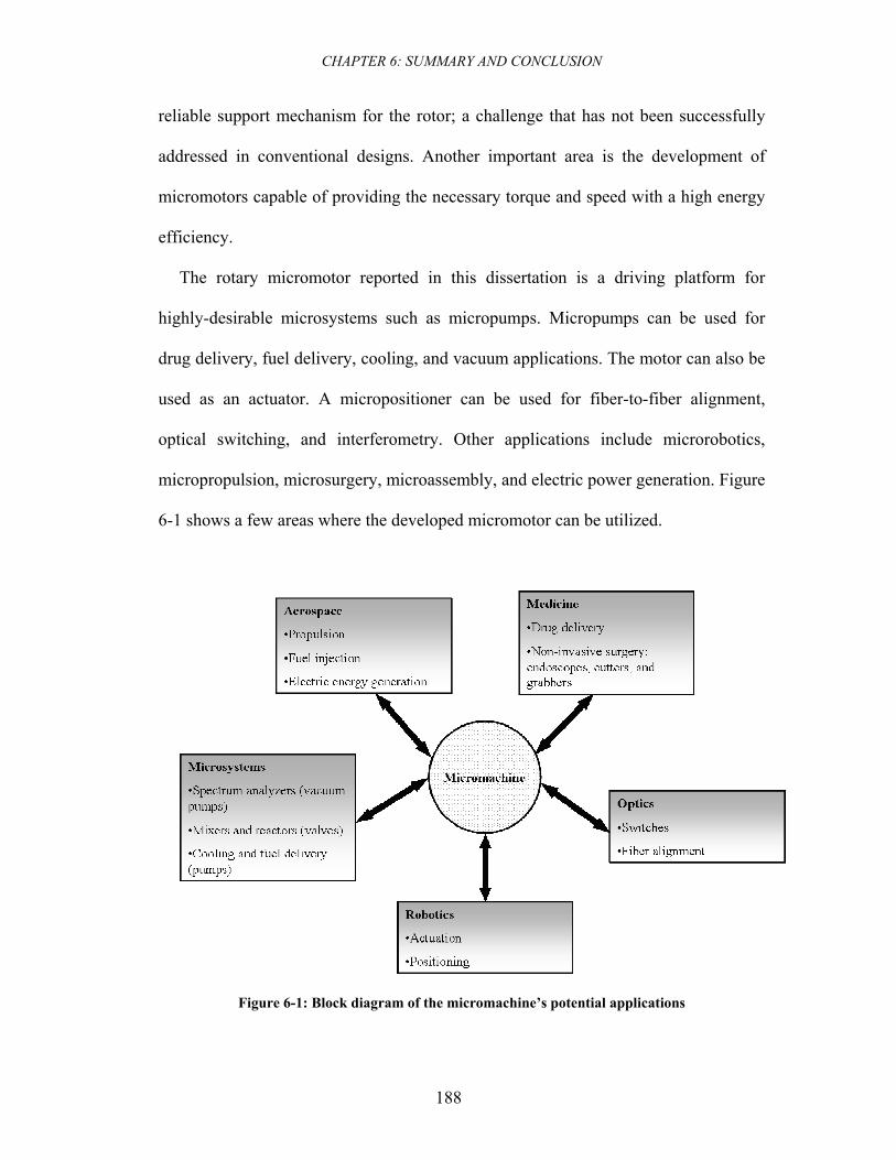
CHAPTER 6: SUMMARY AND CONCLUSION
188
reliable support mechanism for the rotor; a challenge that has not been successfully
addressed in conventional designs. Another important area is the development of
micromotors capable of providing the necessary torque and speed with a high energy
efficiency.
The rotary micromotor reported in this dissertation is a driving platform for
highly-desirable microsystems such as micropumps. Micropumps can be used for
drug delivery, fuel delivery, cooling, and vacuum applications. The motor can also be
used as an actuator. A micropositioner can be used for fiber-to-fiber alignment,
optical switching, and interferometry. Other applications include microrobotics,
micropropulsion, microsurgery, microassembly, and electric power generation. Figure
6-1 shows a few areas where the developed micromotor can be utilized.
Figure 6-1: Block diagram of the micromachine’s potential applications
CHAPTER 6: SUMMARY AND CONCLUSION
189
The implementation of the current design in the above applications requires
additional improvements to the electrical and mechanical designs. In the electrical
domain, a closed-loop excitation system is required for position, speed, and torque
control. A feedback control system will improve the reliability, stability, and
functionality of this synchronous machine. Furthermore, the performance of the
machine is improved with small gap size and large number of electrodes. There are
number of fabrication challenges including gap uniformity that need to be addressed
to achieve gap sizes smaller than 10 μm.
Improvements to the mechanical design are also necessary. Currently,
encapsulated bearings are under development at UMD for centrifugal micropumps
(without a motor) using wafer bonding steps. In these designs, the balls are
encapsulated in housings etched in rotor and stator. The encapsulated bearing can
potentially be used at speeds up to a few hundred thousands of rpm. Moreover, one of
the drawbacks of the current bearing design reported in this dissertation is ball
colocation. Therefore, it is necessary to design and fabricate ball retainer rings to
eliminate microball collisions. Finally, the friction and wear of the microballs and the
housing need to be reduced using dry lubricant films. The geometry of the ball
housing, as well as the coating, needs to be optimized. Tribology experiments are
currently underway in our research group to study the effect of hard coatings such as
silicon carbide and diamond-like-carbon on the friction and wear.
REFERENCES
190
References
[1] X. Wang, S. Cui, and S. Cheng, "Advantages of electrostatic micromotor and its application to medical instruments," presented at Conference Record of the 2002 IEEE Industry Applications, Pittsburgh, PA, USA, 2002.
[2] D. Polla, A. Erdman, D. Peichel, R. Rizq, Y. Gao, and D. Markus, "Precision micromotor for surgery," presented at Proceedings of 1st Annual International IEEE-EMBS Special Topic Conference on Microtechnologies in Medicine and Biology, Lyon, France, 12-14 Oct. 2000.
[3] L. M. Gao, Y. Chen, L. M. Lin, and G. Z. Yan, "Micro motor based new type of endoscope," presented at Proceedings of the 20th Engineering in Medicine and Biology Society, Hong Kong, China, 1998.
[4] D. J. Laser and J. G. Santiago, "A review of micropumps," Journal of Micromechanics and Microengineering, vol. 14, pp. R35, 2004.
[5] T. Weisener, G. Vogele, M. Widmann, C. Bark, R. D. Schraft, A. Bertholds, and A. Braunschweiler, "Development and fabrication of a rotary micropump and its industrial and medical applications," presented at Proceedings of the SPIE, Austin, TX, USA, 1996.
[6] C. H. Ahn and M. G. Allen, "Fluid micropumps based on rotary magnetic actuators," presented at IEEE Microelectromechanical Systems (MEMS '95), Amsterdam, Netherlands, 1995.
[7] B. Mladen, J. M. Jack, P. G. Andrew, and S. Schultz, "Electromagnetic micromotor for microfluidics applications," Applied Physics Letters, vol. 79, pp. 1399-1401, 2001.
[8] S. Fatikow, A. Falzullin, and J. Seyfried, "Planning of a microassembly task in a flexible microrobot cell," presented at Proceedings of the IEEE International Conference on Robotics and Automation (ICRA), San Francisco, CA, USA, 24-28 April, 2000.
[9] R. Yeh, S. Hollar, and K. S. J. Pister, "Design of low-power silicon articulated microrobots," Journal of Micromechatronics, vol. 1, pp. 191, 2002.
[10] R. Yeh, E. J. J. Kruglick, and K. S. J. Pister, "Surface-micromachined components for articulated microrobots," Journal of Microelectromechanical Systems, vol. 5, pp. 10, 1996.
REFERENCES
191
[11] W. S. N. Trimmer and K. J. Gabriel, "Design Consideration for a Practical Electrostatic Micro-motor," Sensors and Actuators, vol. 11, pp. 189-206, 1987.
[12] O. D. Jefimenko and D. K. Walker, Electrostatic motors: their history, types, and principles of operation. Star City, West Virginia: Electret Scientific Company, 1973.
[13] B. Bollee, "Electrostatic Motors," Philips technical review, pp. 178-194, 1969.
[14] J. G. Trump, "Eloctrostatic Sources of Electric Power," Electrical Engineering, vol. 66, pp. 525-534, 1947.
[15] J. G. Trump, "Vaccum Electrostatic Engineering." Cambridge, MA, USA: Massachusetts Institute of Technology, 1933.
[16] M. J. Mulcahy and W. R. Bell, "Electrostatic Generators," in Electrostatic and its application, Chapter 8, 1973, pp. 148-179.
[17] P. L. Chapman and P. T. Krein, "Micromotor technology: Electric drive designer's perspective," presented at Industry application conference annual meeting, Chicago, IL, USA, 2001.
[18] D. P. Arnold, F. Cros, I. Zana, M. G. Allen, S. Das, and J. H. Lang, "Magnetic induction machines embedded in fusion-bonded silicon," presented at Solid-State Sensors, Actuators and Microsystems Workshop, Hilton Head Island, SC, USA, 2004.
[19] S. Das, D. P. Arnold, and M. G. Allen, "Multi-watt electric power from a fabricated permanent-magnet generator," presented at IEEE Micro Electro Mechanical Systems (MEMS '05), Miami, FL, USA, 2005.
[20] K. Dutta, P. Dev, R. Dewilde, B. Sharma, and R. W. Newcomb, "Integrated Micromotor Concepts," Stanford University AFOSR70-1682TR, 1970.
[21] P. L. Chapman and P. T. Krein, "Smaller is better? Micromotors and electric drives," IEEE Industry Applications Magazine, vol. 9, pp. 62, 2003.
[22] J. Boland, Y.-H. Chao, Y. Suzuki, and Y. C. Tai, "Micro electret power generator," presented at IEEE Sixteenth Annual International Conference on Micro Electro Mechanical Systems, MEMS-03, Kyoto, Japan, 2003.
REFERENCES
192
[23] J. Boland, H. W. Messenger, H. W. Lo, and Y. C. Tai, "Arrayed liquid rotor electret power generator systems," presented at IEEE Micro Electro Mechanical Systems (MEMS '05), Miami, FL, USA, 2005.
[24] T. Sterken, P. Fiorini, K. Baert, R. Puers, and G. Borghs, "An electret-based electrostatic μ-generator," presented at 12th International Conference on, TRANSDUCERS, Solid-State Sensors, Actuators and Microsystems, Boston, MA, USA, 2003.
[25] S. Tanaka, T. Genda, and M. Esashi, "High power electrostatic motor and generator using electrets," presented at 12th International Conference on,TRANSDUCERS, Solid-State Sensors, Actuators and Microsystems, Boston, MA, USA, 2003.
[26] Y. B. Jeon, R. Sood, J. H. Jeong, and S. G. Kim, "MEMS power generator with transverse mode thin film PZT," Sensors and Actuators, vol. in press, 2005.
[27] R. Sood and S. G. Kim, "Piezoelectric micro power generation for energy harvesting," presented at Solid-State Sensors, Actuators and Microsystems Workshop, Hilton Head Island, SC, USA, 2004.
[28] S. Cagatay, B. Koc, P. Moses, and K. Uchino, "A piezoelectric micromotor with a stator of phi =1.6mm and l=4 mm using bulk PZT," Japanese Journal of Applied Physics, Part 1, vol. 43, pp. 1429-1433, 2004.
[29] J. Friend, K. Nakamura, and S. Ueha, "A piezoelectric micromotor using in-plane shearing of PZT elements," IEEE/ASME Transactions on Mechatronics, vol. 9, pp. 467-473, 2004.
[30] S. Dong, S. P. Lim, K. H. Lee, J. Zhang, L. C. Lim, and K. Uchino, "Piezoelectric ultrasonic micromotor with 1.5 mm diameter," IEEE Transactions on Ultrasonics, Ferroelectrics and Frequency Control, vol. 50, pp. 361-367, 2003.
[31] J. T. Leinvuo, S. A. Wilson, H. J. A. Almond, and R. W. Whatmore, "Experimental design and construction of a flextensional ultrasonic piezoelectric micro-motor," presented at Tenth European Meeting on Ferroelectricity, Cambridge, UK, 2004.
[32] L. S. Fan, Y. C. Tai, and R. S. Muller, "IC-processed electrostatic micro-motors," presented at Technical Digest of International Electron Devices Meeting, San Francisco, CA, USA, 1988.
REFERENCES
193
[33] Y. C. Tai, L. S. Fan, and R. S. Muller, "IC processed micro-motors: design, technology, and testing," presented at Proceedings of Micro Electro Mechanical Systems, Salt Lake City, UT, 1989.
[34] M. Mehregany, S. F. Bart, L. S. Tavrow, J. H. Lang, and S. D. Senturia, "Principles in design and microfabrication of variable-capacitance side-drive motors," Journal of Vacuum Science & Technology A, vol. 8, pp. 3614-3624, 1990.
[35] J. M. Bustillo, R. T. Howe, and R. S. Muller, "Surface micromachining for microelectromechanical systems," Proceedings of the IEEE, vol. 86, pp. 1552-1574, 1998.
[36] H. C. Nathanson, W. E. Newell, R. A. Wickstrom, and J. R. Davis, Jr., "The resonant gate transistor," Electron Devices, IEEE Transactions on, vol. 14, pp. 117, 1967.
[37] T. A. Lober, "A microfabricated electrostatic motor design and process." Cambridge, MA: Massachusetts Institute of Technology, 1988.
[38] L. S. Fan, Y. C. Tai, and R. S. Muller, "Integrated movable micromechanical structures for sensors and actuators," IEEE Transactions on Electron Devices, vol. 35, pp. 724, 1988.
[39] M. Mehregany, K. J. Gabriel, and W. S. N. Trimmer, "Integrated fabrication of polysilicon mechanisms," IEEE Transactions on Electron Devices, vol. 35, pp. 719, 1988.
[40] M. Mehregany, S. F. Bart, L. S. Tavrow, J. H. Lang, and S. D. Senturia, "Principles in design and microfabrication of variable-capacitance side-drive motors," Journal of Vacuum Science & Technology A: Vacuum, Surfaces, and Films, vol. 8, pp. 3614-3624, 1990.
[41] M. Mehregany, S. D. Senturia, J. H. Lang, and P. Nagarkar, "Micromotor fabrication," IEEE Transactions on Electron Devices, vol. 39, pp. 2060, 1992.
[42] F. Long-Sheng, T. Yu-Chong, and R. S. Muller, "IC-processed electrostatic micro-motors," presented at Technical Digest of International Electron Devices Meeting, San Francisco, CA, USA, 1988.
[43] M. Mehregany, S. D. Senturia, and J. H. Lang, "Measurement of wear in polysilicon micromotors," IEEE Transactions on Electron Devices, vol. 39, pp. 1136, 1992.
REFERENCES
194
[44] M. Mehregany, S. D. Senturia, and J. H. Lang, "Friction and wear in microfabricated harmonic side-drive motors," presented at IEEE Solid-State Sensor and Actuator Workshop Technical Digest, Hilton Head Island, SC, USA, 1990.
[45] V. R. Dhuler, M. Mehregany, and S. M. Phillips, "Micromotor operation in a liquid environment," presented at IEEE Solid-State Sensor and Actuator Workshop Technical Digest, Hilton Head Island, SC, USA, 1992.
[46] A. Azzam Yasseen, J. N. Mitchell, D. A. Smith, and M. Mehregany, "High-aspect-ratio rotary polygon micromotor scanners," Sensors and Actuators A: Physical, vol. 77, pp. 73-79, 1999.
[47] A. Azzam Yasseen, J. N. Mitchell, J. F. Klemic, D. A. Smith, and M. Mehregany, "A rotary electrostatic micromotor 1 times 8 optical switch," Journal of Selected Topics in Quantum Electronics, vol. 5, pp. 26-32, 1999.
[48] V. D. Samper, A. J. Sangster, R. L. Reuben, and U. Wallrabe, "Multistator LIGA-fabricated electrostatic wobble motors with integrated synchronous control," Journal of Microelectromechanical Systems, vol. 7, pp. 214, 1998.
[49] A. Azzam Yasseen, W. Chien Hung, C. A. Zorman, and M. Mehregany, "Fabrication and testing of surface micromachined polycrystalline SiC micromotors," Electron Device Letters, IEEE, vol. 21, pp. 164, 2000.
[50] A. Azzam Yasseen, W. Chien-Hung, C. A. Zorman, and M. Mehregany, "Fabrication and testing of surface micromachined silicon carbide micromotors," presented at Proceedings of 12th International Workshop on Micro Electro Mechanical Systems (MEMS'99), Orlando, FL, USA, 17-21 Jan,1999.
[51] W. Zhang, G. Meng, and H. Li, "Electrostatic micromotor and its reliability," Microelectronics Reliability, vol. 45, pp. 1230, 2005.
[52] R. Agrawal, Q. Hasan, N. Ashraf, K. B. Sundaram, L. C. Chow, J. S. Kapat, and J. Vaidya, "Design and fabrication of meso-scale variable capacitance motor for miniature heat pumps," Journal of Microemechanics and Microengineering, vol. 13, pp. 1-7, 2002.
[53] K. Noguchi, H. Fujita, M. Suzuki, and N. Yoshimura, "The measurements of friction on micromechatronics elements," presented at IEEE Micro Electro Mechanical Systems (MEMS'91), Nara, Japan, 1991.
REFERENCES
195
[54] K. Deng, W. H. Ko, and G. M. Michal, "A preliminary study on friction measurements in MEMS," presented at International Conference on Solid-State Sensors and Actuators, Digest of Technical Papers (TRANSDUCERS '91), San Francisco, CA, USA, 1991.
[55] J. U. Jeon, S. J. Woo, and T. Higuchi, "Variable-capacitance motors with electrostatic suspension," Sensors and Actuators A: Physical, vol. 75, pp. 289, 1999.
[56] C. B. Williams, C. Shearwood, P. H. Mellor, and R. B. Yates, "Modelling and testing of a frictionless levitated micromotor," Sensors and Actuators A: Physical, vol. 61, pp. 469, 1997.
[57] C. Shearwood, K. Y. Ho, C. B. Williams, and H. Gong, "Development of a levitated micromotor for application as a gyroscope," Sensors and Actuators A: Physical, vol. 83, pp. 85, 2000.
[58] X. S. Wu, W. Y. Chen, X. L. Zhao, and W. P. Zhang, "Micromotor with electromagnetically levitated rotor using separated coils," Electronics Letters, vol. 40, pp. 996.
[59] C. Ruffert, R. Gehrking, B. Ponick, and H. H. Gatzen, "Magnetic Levitation Assisted Guide for a Linear Micro-Actuator," Magnetics, IEEE Transactions on, vol. 42, pp. 3785, 2006.
[60] W. Chien-Chang, Y. Yeong-Der, L. Chien-Sheng, and C. Lung-Yu, "Micro-magnetic suspension motor design for miniature optical drive," Japanese Journal of Applied Physics, Part 1 (Regular Papers, Short Notes & Review Papers), vol. 45, pp. 5801.
[61] C. Livermore, A. R. Forte, T. Lyszczarz, S. D. Umans, A. A. Ayon, and J. H. Lang, "A high-power MEMS electric induction motor," Journal of Microelectromechanical Systems, vol. 13, pp. 465-471, 2004.
[62] J. L. Steyn and J. H. Lang, "Generating electric power with a MEMS electroquasistatic induction turbine-generator," presented at IEEE Microel ectro mechanical systems (MEMS '05), Miami, FL, USA, 2005.
[63] C. H. Ahn, Y. J. Kim, and M. G. Allen, "A planar variable reluctance magnetic micromotor with fully integrated stator and coils," Journal of Microelectromechanical Systems, vol. 2, pp. 165-173, 1993.
REFERENCES
196
[64] C. H. Ahn, Y. J. Kim, and M. G. Allen, "A planar variable reluctance magnetic micromotor with fully integrated stator and wrapped coils," presented at IEEE micro electro mechanical systems (MEMS '93), Fort Lauderdale, FL, USA, 1993.
[65] D. P. Arnold, F. Cros, I. Zana, D. R. Veazie, and M. G. Allen, "Electroplated metal microstructures embedded in fusion-bonded silicon: conductors and magnetic materials," Journal of Microelectromechanical Systems, vol. 13, pp. 791, 2004.
[66] H. Koser and J. H. Lang, "Magnetic induction micromachine-part I: Design and analysis," Microelectromechanical Systems, Journal of, vol. 15, pp. 415, 2006.
[67] F. Cros, H. Koser, M. G. Allen, and J. H. Lang, "Magnetic induction micromachine-part II: fabrication and testing," Microelectromechanical Systems, Journal of, vol. 15, pp. 427, 2006.
[68] H. Koser and J. H. Lang, "Magnetic induction micromachine-part III:Eddy currents and nonlinear effects," Microelectromechanical Systems, Journal of, vol. 15, pp. 440, 2006.
[69] T. W. Krygowski, M. S. Rodgers, J. Sniegowski, S. M. Miller, and J. Jakubczak, "A low-voltage rotary actuator fabricated using a five-level polysilicon surface micromachining technology," presented at International Electron Devices Meeting (IEDM), Washington, DC, 1999.
[70] B. C. Yen and J. H. Lang, "A Variable-Capacitance Vibration-to-electric Energy Harvester," Submitted to IEEE Transactions on Circuits and Systems I, 2005.
[71] M. Miyazaki, H. Tanaka, G. Ono, T. Nagano, N. Ohkubo, and T. Kawahara, "Electric-energy generation through variable-capacitive resonator for power-free LSI," IEICE Transactions on Electronics, vol. E87-C, pp. 549-555, 2004.
[72] P. Glynne-Jones, M. J. Tudor, S. P. Beeby, and N. M. White, "An electromagnetic, vibration-powered generator for intelligent sensor systems," Sensors and Actuators A: Physical, vol. 110, pp. 344-349, 2004.
[73] D. P. Arnold, H. Florian, Z. Iulica, G. Preston, P. Jin-Woo, D. Sauparna, H. L. Jeffrey, and G. A. Mark, "Design optimization of an 8 W, microscale, axial-flux, permanent-magnet generator," Journal of Micromechanics and Microengineering, vol. 16, pp. S290, 2006.
REFERENCES
197
[74] D. P. Arnold, S. Das, J. W. Park, I. Zana, J. H. Lang, and M. G. Allen, "Microfabricated High-Speed Axial-Flux Multiwatt Permanent-Magnet Generators; Part II: Design, Fabrication, and Testing," Microelectromechanical Systems, Journal of, vol. 15, pp. 1351, 2006.
[75] S. Das, D. P. Arnold, I. Zana, J. W. Park, M. G. Allen, and J. H. L. Lang, "Microfabricated High-Speed Axial-Flux Multiwatt Permanent-Magnet Generators; Part I: Modeling," Microelectromechanical Systems, Journal of, vol. 15, pp. 1330, 2006.
[76] T. C. Neugebauer, D. J. Perreault, J. H. Lang, and C. Livermore, "A six-phase multilevel inverter for MEMS electrostatic induction micromotors," IEEE Transactions on Circuits and Systems II: Express Briefs, vol. 51, pp. 49, 2004.
[77] S. L. Garverick, M. L. Nagy, N. K. Rao, D. K. Hartsfield, and A. Purushotham, "A capacitive sensing integrated circuit for detection of micromotor critical angles," IEEE Journal of Solid-State Circuits, vol. 32, pp. 23, 1997.
[78] J. T. Horstmann and K. F. Goser, "Monolithic integration of a silicon micromotor in combination with the CMOS drive circuit on one chip," Microelectronic Engineering, vol. 67-68, pp. 390, 2003.
[79] S. F. Bart, "Modeling and design of electroquasistatic microactuators.," in Dept. of Electrical Engineering and Computer Science. Cambridge, MA, USA: Massachusetts Institute of Technology, 1990.
[80] S. F. Bart, M. Mehregany, L. S. Tavrow, J. H. Lang, and S. D. Senturia, "Electric micromotor dynamics," IEEE Transactions on Electron Devices, vol. 39, pp. 566, 1992.
[81] K. C. Stark, M. Mehregany, and S. M. Phillips, "Mechanical coupling and direct torque measurement of outer-rotor polysilicon micromotors," presented at Proceedings IEEE, The Tenth Annual International Workshop on Micro Electro Mechanical Systems., An Investigation of Micro Structures, Sensors, Actuators, Machines and Robots, New York, NY, USA, 1997.
[82] K. C. Stark, A. Azzam Yasseen, S. M. Phillips, and M. Mehregany, "Micro torque measurement using outer-rotor polysilicon micromotors," presented at Proceedings of IEEE Sensors, Orlando, FL, USA, 2002.
[83] A. Modafe, N. Ghalichechian, J. H. Lang, and R. Ghodssi, "A Microball-Bearing-Supported Linear Electrostatic Micromotor with Benzocyclobutene Polymer Insulating Layers," presented at The 13th International Conference
REFERENCES
198
on Solid-State Sensors, Actuators, and Microsystems (Transducers '05), Seoul, Korea, 2005.
[84] A. Modafe, "Benzocyclobutene-Based Electric Micromachines Supported on Microball Bearings: Design, Fabrication, and Characterization," in Deprtment of Electrical and Computer Engineering. Collge Park, MD, USA: University of Maryland, 2007.
[85] L. G. Frechette, S. A. Jacobson, K. S. Breuer, F. F. Ehrich, R. Ghodssi, R. Khanna, W. Chee Wei, Z. Xin, M. A. Schmidt, and A. H. Epstein, "High-speed microfabricated silicon turbomachinery and fluid film bearings," Journal of Microelectromechanical Systems, vol. 14, pp. 141, 2005.
[86] A. Modafe, N. Ghalichechian, M. Powers, M. Khbeis, and R. Ghodssi, "Embedded benzocyclobutene in silicon: An integrated fabrication process for electrical and thermal isolation in MEMS," Microelectronic Engineering, vol. 82, pp. 154, 2005.
[87] A. Modafe, "Benzocyclobutene-Based Electric Micromachines Supported on Microball Bearings: Design, Fabrication, and Characterization," in Deaprtment of Electrical and Computer Engineering. Collge Park, MD, USA: University of Maryland, 2006.
[88] L. Ta-Wei, A. Modafe, B. Shapiro, and R. Ghodssi, "Characterization of dynamic friction in MEMS-based microball bearings," Instrumentation and Measurement, IEEE Transactions on, vol. 53, pp. 839, 2004.
[89] A. Modafe, N. Ghalichechian, B. Kleber, and R. Ghodssi, "Electrical characterization of Benzocyclobutene polymers for electric micro machines," IEEE Transactions on Device and Materials Reliability, vol. 4, pp. 495-508, 2004.
[90] N. Ghalichechian, A. Modafe, P. Lazzeri, V. Micheli, M. Anderle, and R. Ghodssi, "Characterization of Benzocyclobutene and Chromium-gold Film Interface for Application in Silicon Micromachining," presented at Material Research Society 2005 Spring Meeting, San Francisco, CA, USA, 28-April 1, 2005.
[91] N. Ghalichechian, A. Modafe, and R. Ghodssi, "Integration of Silicon Anisotropic Wet Etching and BCB Processes," presented at AVS 50th International Symposium, Baltimore, MD, USA, November 2-7, 2003.
[92] N. Ghalichechian, "Integration of Benzocyclobutene Polymers and Silicon Micromachines Structures Fabricated with Anisotropic Wet Etching," in
REFERENCES
199
Department of Electrical and Computer Engineering. College Park, MD, USA: University of Maryland, 2004.
[93] N. Ghalichechian, A. Modafe, R. Ghodssi, P. Lazzeri, V. Micheli, and M. Anderle, "Integration of Benzocyclobutene Polymers and Silicon Micromachined Structures Using Anisotropic Wet Etching," Journal of Vacuum Science & Technology B, vol. 22, pp. 2439-244, 2004.
[94] M. J. Madou, Fundamentals of microfabrication the science of miniaturization, 2nd ed. Boca Raton: CRC Press, 2002.
[95] R. A. Kirchhoff and K. J. Bruza, "Benzocyclobutenes in polymer synthesis," Progress in Polymer Science, vol. 18, pp. 85-185, 1993.
[96] M. F. Farona, "Benzocyclobutenes in polymer chemistry," Progress in Polymer Science, vol. 21, pp. 505-555, 1996.
[97] M. E. Mills, P. Townsend, D. Casrillo, S. Martin, and A. Achen, "Benzocyclobutene (DVS-BCB) polymer as an interlayer dielectric (ILD) material," Microelectronic Engineering, vol. 33, pp. 327-334, 1997.
[98] "Processing procedures for dry-etch CYCLOTENE advance electronics resins (dry-etch BCB)," Dow Chemical, 2004.
[99] P. B. Chinoy and J. Tajadod, "Processing and microwave characterization of multilevel interconnects using benzocyclobutene dielectric," IEEE Transactions on Components, Hybrids, and Manufacturing Technology, vol. 16, pp. 714-719, 1993.
[100] A. J. G. Strandjord, R. H. Heistand, P. Garrou, and T. G. Tessier, "A photosensitive-BCB on laminate technology (MCM-LD)," presented at 44th Electronic Components and Technology Conference, Washington DC, USA, 1994.
[101] D. C. Burdeaux, P. H. Townsend, J. N. Carr, and P. Garrou, "Benzocyclobutene (BCB) dielectrics for the fabrication of high density, thin film multichip modules," Journal of Electronic Materials, vol. 19, pp. 1357-1366, 1990.
[102] M. J. Berry, T. G. Tessier, I. Turlik, G. M. Adema, D. C. Burdeaux, J. N. Carr, and P. Garrou, "Benzocyclobutene as a dielectric for multichip module fabrication," presented at 40th Electronic Components and Technology Conference, 1990.
REFERENCES
200
[103] R. D. Sandell, G. Akerling, and A. D. Smith, "Multi-chip packaging for high speed superconducting circuits," presented at Applied Superconductivity Conference, Boston, MA, USA, 1995.
[104] T. Miyagi, Y. Iseki, K. Higuchi, Y. Shizuki, T. Hanawa, E. Takagi, M. Saito, K. Yoshihara, and M. Konno, "MCM-D/L using copper/photosensitive-BCB multilayer for upper microwave band systems," presented at 46th Electronic Components and Technology Conference, Orlando, FL, USA, 1996.
[105] Y. Ida, P. E. Garrou, A. J. G. Strandjord, S. L. Cummings, W. B. Rogers, M. J. Berry, and S. R. Kisting, "Processing, transfer solder bumping, chip attachment and testing of a thin film Cu/photo-BCB MCM-D," presented at 8th IEEE/CPMT Int. Electronic Manufacturing Technology Symp., Japan, 1995.
[106] L. A. Keser, R. Bajaj, and T. Fang, "Redistribution and bumping of a high I/O device for flip chip assembly," IEEE Transactions on Advanced Packaging, vol. 23, pp. 3-8, 2000.
[107] D. T. Price, R. J. Gutmann, and S. P. Murarka, "Damascene copper interconnects with polymer ILDs," presented at 24th International Conference on Metallurgical Coatings and Thin Films, Switzerland San Diego, CA, USA, 1997.
[108] A. J. G. Strandjord, W. B. Rogers, Y. Ida, R. R. De Vellis, S. Shiau, E. S. Moyer, D. M. Scheck, and P. E. Garrou, "Photosensitive benzocyclobutene for stress-buffer and passivation applications (one mask manufacturing process)," presented at 47th Electronic Components and Technology Conference, San Jose, CA, 1997.
[109] X. Huo, K. J. Chen, and P. C. H. Chan, "High-Q copper inductors on standard silicon substrate with a low-k BCB dielectric layer," presented at Proceedings of 2002 International Microwave Symposium, Seattle, WA, USA, 2002.
[110] C. F. Kane and R. R. Krchnavek, "Benzocyclobutene optical waveguides," IEEE Photonics Technology Letters, vol. 7, pp. 535-537, 1995.
[111] S. Wolff, A. R. Giehl, M. Renno, and H. Fouckhardt, "Metallic waveguide mirrors in polymer film waveguides," presented at 10th European Conference on Integrated Optics, Paderborn, Germany, 2001.
[112] C. Laville, C. Pellet, and G. N'Kaoua, "Interdigitated humidity sensors for a portable clinical microsystem," presented at 1st Ann. Int. IEEE-EMBS Special Topic Conf. Microtechnologies in Medicine and Biology, Lyon, France, 2000.
REFERENCES
201
[113] H. H. Gatzen, E. Obermeier, T. Kohlmeier, T. Budde, H. D. Ngo, B. Mukhopadhya, and M. Farr, "An electromagnetically actuated bi-stable mems optical microswitch," presented at 12th International Conference on TRANSDUCERS, Solid-State Sensors, Actuators and Microsystems, Boston, MA, USA, 2003.
[114] P. Turmezei, A. Polyakov, J. R. Mollinger, M. Bartek, A. Bossche, and J. N. Burghartz, "Low-cost microfilter for red blood cell membrane stiffness measurement using photosensitive bcb," presented at 12th Innational Conference on Solid-State Sensors, Actuators and Microsystems, Boston, MA, USA, 2003.
[115] A. Jourdain, X. Rottenberg, G. Carchon, and H. A. C. Tilmans, "Optimization of 0-level packaging for RF-MEMS devices," presented at 12th Innational Conference on TRANSDUCERS, Solid-State Sensors, Actuators and Microsystems, Boston, MA, USA, 2003.
[116] F. Niklaus, H. Andersson, P. Enoksson, and G. Stemme, "Low temperature full wafer adhesive bonding of structured wafers," presented at Proceedings of EUROSENSORS, Switzerland Copenhagen, Denmark, 2001.
[117] T.-K. A. Chou and K. Najafi, "3D MEMS fabrication using low-temperature wafer bonding with benzocyclobutene (BCB)," presented at Solid-State Sensors and Actuators 11th International Conference, Munich, Germany, 2001.
[118] J. Oberhammer and G. Stemme, "Incrementally etched electrical feedthroughs for wafer-level transfer of glass lid packages," presented at Solid-State Sensors, Actuators and Microsystems 12th Innational Conference, Boston, MA, USA, 2003.
[119] J. M. Snodgrass and R. H. Dauskardt, "The effect of fatigue on the adhesion and subcritical debonding of benzocyclobutene/silicon dioxide interfaces," presented at Materials, Technology and Reliability for Advanced Interconnects and Low-k Dielectrics Symposium, San Francisco, CA, USA, 2001.
[120] J. M. Snodgrass, D. Pantelidis, M. L. Jenkins, J. C. Bravman, and R. H. Dauskardt, "Subcritical debonding of polymer/silica interfaces under monotonic and cyclic loading," Acta Materialia, vol. 50, pp. 2395-2411, 2002.
[121] J. Im, E. O. Shaffer, R. Peters, T. Rey, C. Murlick, and R. L. Sammler, "Physical and mechanical properties determination of photo-BCB-based thin films," presented at International Symposium on Microelectronics, 1996.
REFERENCES
202
[122] J.-h. Im, E. O. Shaffer, II, T. Stokich, Jr, A. Strandjord, J. Hetzner, J. Curphy, C. Karas, G. Meyers, D. Hawn, A. Chakrabarti, and S. Froelicher, "On the mechanical reliability of photo-BCB-based thin film dielectric polymer for electronic packaging applications," Transactions of the ASME. Journal of Electronic Packaging, vol. 122, pp. 28-33, 2000.
[123] J. T. Beechinor, E. McGlynn, M. O'Reilly, and G. M. Crean, "Optical characterisation of thin film benzocyclobutene (BCB) based polymers," presented at Advanced Materials for Interconnections Symposium, E-MRS Spring Meeting Conference, Netherlands Strasbourg, France, 1997.
[124] S. Guo, "Cyclotene(R) diaphragm for MEMS-based IR detectors," presented at Proceedings of the SPIE - The International Society for Optical Engineering, Micromachining and Microfabrication Process Technology VII, USA San Jose, CA, USA, 2003.
[125] C. L. Borst, D. G. Thakurta, W. N. Gill, and R. J. Gutmann, "Chemical-mechanical planarization of low-k polymers for advanced IC structures," Transactions of the ASME, Journal of Electronic Packaging, vol. 124, pp. 362-366, 2002.
[126] F. Kuchenmeister, Z. Stavreva, U. Schubert, K. Richter, C. Wenzel, and M. Simmonds, "A comparative CMP study of BCB and SiLK for copper damascene technologies," presented at Advanced Metallization Conference, Colorado Springs, CO, USA, 1998.
[127] A. Modafe, N. Ghalichechian, A. Frey, J. H. Lang, and R. Ghodssi, "Microball-Bearing-Supported Electrostatic Micromachines with Polymer Dielectric Films for Electromechanical Power Conversion," Journal of Micromechanics and Microengineering, vol. 16, pp. S182-S190, 2006.
[128] S. D. Senturia, Microsystem design. Boston: Kluwer Academic Publishers, 2001.
[129] J. D. Jackson, Classical Electrodynamics, 3rd ed. New York: John Wiley and Sons, 1998.
[130] A. Modafe, N. Ghalichechian, A. Frey, J. H. Lang, and R. Ghodssi, "Microball-Bearing-Supported Electrostatic Micromachines with Polymer Dielectric Films for Electromechanical Power Conversion," presented at The fifth International Workshop on Micro NanoTechnology for Power Generation and Energy Conversion Applications (Power MEMS '05), Tokyo, Japan, 2005.
REFERENCES
203
[131] A. Modafe, N. Ghalichechian, A. Frey, J. H. Lang, and R. Ghodssi, "Microball-Bearing-Supported Electrostatic Micromachines with Polymer Dielectric Films for Electromechanical Power Conversion," Journal of Micromechanics and Microengineering, In Press, 2006.
[132] N. Ghalichechian, A. Modafe, A. Frey, J. H. Lang, and R. Ghodssi, "Dynamic Characterization of a Linear Variable-Capacitance Micromotor," presented at Solid-State Sensor, Actuator, and Microsystems Workshop, Hilton Head Island, SC, USA, June 4-8, 2006.
[133] A. Modafe, N. Ghalichechian, J. H. Lang, and R. Ghodssi, "A Microball-Bearing-Supported Linear Electrostatic Micromotor with Benzocyclobutene Polymer Insulating Layers," presented at The 13th International Conference on Solid-State Sensors, Actuators, and Microsystems (Transducers '05), Seoul, Korea, 2005.
[134] M. McCarthy, B. Hanrahan, C. Zorman, and R. Ghodssi, "Rolling Friction in MEMS Ball Bearings: The Effects of Loading and Solid Film Lubrication," presented at ASME/STLE International Joint Tribology Conference, San Diego, CA, USA, 2007.