Uncertainty about the Persistence of Periods with Large Price Shocks and the Optimal Reaction of the Monetary Authority

Arnulfo Rodriguez*

Jesus R. Gonzalez-Garcia*

Fidel Gonzalez∗∗

Preliminary version: May, 2005

* Dirección General de Investigación Económica, Banco de México. We thank Daniel Chiquiar, Alejandro Gaytán, Rodrigo García and Othón Moreno for very useful comments and Brenda Jarillo Rabling and Lorenzo E. Bernal Verdugo for excellent research assistance. The opinions in this paper correspond to the authors and do not necessarily reflect the point of view of Banco de México. ∗∗ Subdirección de Estudios Económicos de Vivienda, Sociedad Hipotecaria Federal. The opinions in this paper correspond to the author and do not necessarily reflect the point of view of Sociedad Hipotecaria Federal.

Uncertainty about the Persistence of Periods with Large Price Shocks and the Optimal Reaction of the Monetary Authority

Arnulfo Rodriguez

Jesus R. Gonzalez-Garcia

Fidel Gonzalez

Preliminary version: May, 2005

Abstract. Uncertainty about the persistence of periods characterized by large price shocks is an important aspect of monetary policy. This type of uncertainty posed some difficulties for central banks in 2004. This paper formalizes the treatment of this type of uncertainty by solving an optimal control problem in which the economy randomly alternates between two regimes characterized by different magnitudes of price shocks. By using an open economy model, we find that the optimal policy rule is both regime-contingent and robust. In particular, we find that: a) the optimal reaction of the interest rate is dependent on both the current regime and on the difference in the magnitude of the shocks between regimes; and b) after a robust selection of transition probabilities, the min-max probability of switching to the regime with large price shocks increases when such regime is more harmful. In general, cautious behavior renders smaller losses than recklessness for the monetary authority. This result argues in favor of caution over recklessness in the formulation of monetary policy when there is uncertainty about the persistence of periods with large price shocks.

JEL Classification: C61, E61

Keywords: macroeconomic policy, model uncertainty, optimal control, robustness, Markov regime-switching, monetary policy, inflation targeting.

1

1. Introduction

A motivation for the study developed in this paper can be found in the experience of

several countries in 2004. This year was marked by increases in international prices of

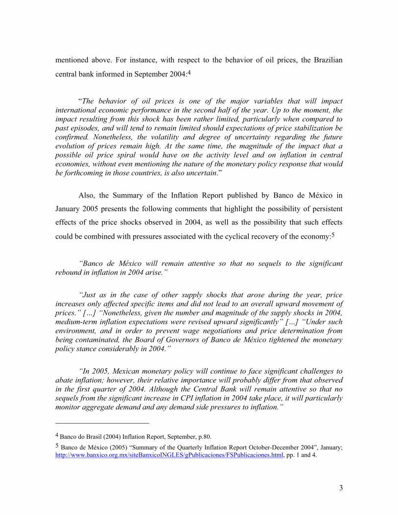
commodities (or primary goods) that affected inflation rates in many economies. Figure 1

shows different indexes of commodity prices in international markets. The shocks to

commodities prices were the result of an increase in the global demand for these goods and

prompted a cautious behavior of many central banks in the face of increasing rates of

inflation throughout the year.1 Figure 2 presents the annual inflation rates in different

regions and countries, which show an increase in 2004.

Figure 12. Indexes of Commodity Prices 2000-2004 (2000=100)

65

85

105

125

145

165

2000

.01

2000

.05

2000

.09

2001

.01

2001

.05

2001

.09

2002

.01

2002

.05

2002

.09

2003

.01

2003

.05

2003

.09

2004

.01

2004

.05

2004

.09

All Commodities Index

Non-fuel Commodities Index

Food

Agricultural Raw Materials

Oil

1 The word caution used here refers to taking relatively more aggressive policy actions. 2 Source: IMF Primary Commodity Prices Tables, elaborated by the Commodities Unit of the Research Department. All Commodities price index includes both Fuel and Non-Fuel price indices. Fuel price index includes Crude Oil, Natural Gas, and Coal price indices. Non-Fuel price index includes Food and Beverages and Industrial Inputs. Food Price Index includes Cereal, Vegetable Oils, Meat, Seafood, Sugar, Bananas, and Oranges. Agricultural Raw Materials price index includes Timber, Cotton, Wool, Rubber, and Hides price indices. Oil index is the 3 Spot Price index, a simple average of the spot prices of Dated Brent, West Texas Intermediate and Dubai Fateh.

2

Figure 23. Annual Rates of Headline Inflation (Per Cent)

-1.0

1.0

3.0

5.0

7.0

9.0

11.0

13.0

15.0

17.0

2000

.01

2000

.05

2000

.09

2001

.01

2001

.05

2001

.09

2002

.01

2002

.05

2002

.09

2003

.01

2003

.05

2003

.09

2004

.01

2004

.05

2004

.09

2005

.01

World

United States

Euro Area

Mexico

Chile

Brazil

The cautious approach adopted by several monetary authorities in the face of the

shocks described above was due to the following reasons:

a) the direct impact of higher commodity prices on inflation rates;

b) the uncertainty about the evolution of commodity prices in the future;

c) the possibility of second round effects of the aforementioned shocks on the process

of price formation; and

d) the possibility of undesirable effects on inflation derived from the combination of

continuing increases in commodity prices and the recovery experienced by the

global economy.

Several monetary authorities expressed caution in the face of the direct effects of

the shocks to commodities prices and the likely ultimate effects because of the reasons

3 Annual inflation rates on consumer prices were obtained from the IMF International Financial Statistics database (monthly data).

3

mentioned above. For instance, with respect to the behavior of oil prices, the Brazilian

central bank informed in September 2004:4

“The behavior of oil prices is one of the major variables that will impact international economic performance in the second half of the year. Up to the moment, the impact resulting from this shock has been rather limited, particularly when compared to past episodes, and will tend to remain limited should expectations of price stabilization be confirmed. Nonetheless, the volatility and degree of uncertainty regarding the future evolution of prices remain high. At the same time, the magnitude of the impact that a possible oil price spiral would have on the activity level and on inflation in central economies, without even mentioning the nature of the monetary policy response that would be forthcoming in those countries, is also uncertain.”

Also, the Summary of the Inflation Report published by Banco de México in

January 2005 presents the following comments that highlight the possibility of persistent

effects of the price shocks observed in 2004, as well as the possibility that such effects

could be combined with pressures associated with the cyclical recovery of the economy:5

“Banco de México will remain attentive so that no sequels to the significant rebound in inflation in 2004 arise.”

“Just as in the case of other supply shocks that arose during the year, price increases only affected specific items and did not lead to an overall upward movement of prices.” […] “Nonetheless, given the number and magnitude of the supply shocks in 2004, medium-term inflation expectations were revised upward significantly” […] “Under such environment, and in order to prevent wage negotiations and price determination from being contaminated, the Board of Governors of Banco de México tightened the monetary policy stance considerably in 2004.”

“In 2005, Mexican monetary policy will continue to face significant challenges to abate inflation; however, their relative importance will probably differ from that observed in the first quarter of 2004. Although the Central Bank will remain attentive so that no sequels from the significant increase in CPI inflation in 2004 take place, it will particularly monitor aggregate demand and any demand side pressures to inflation.”

4 Banco do Brasil (2004) Inflation Report, September, p.80. 5 Banco de México (2005) “Summary of the Quarterly Inflation Report October-December 2004”, January; http://www.banxico.org.mx/siteBanxicoINGLES/gPublicaciones/FSPublicaciones.html, pp. 1 and 4.

4

It was the environment described above that gave way to one of the main worries

present in the elaboration of monetary policy in 2004, namely, the uncertainty about the

persistence of periods with large price shocks.

Walsh (2004) presents some reflections about the concerns faced by central bankers

when shocks to inflation are more persistent. After noting that shocks to the inflation rate

present central bankers with a trade-off between inflation stabilization and output gap

stabilization, he remarks that the problems arising from unexpected shocks become more

serious if the shocks are more lasting. Consequently, central bankers who desire a robust

policy will react to all inflation shocks as if they were going to be more persistent.

In this paper we try to formalize the treatment of uncertainty about the persistence

of shocks to the inflation rate and derive an optimal policy response.

In our framework, the economy randomly alternates between two regimes. The

difference between the two regimes is only due to the magnitude of price shocks. A

convenient way to model the possibility of sudden changes in the magnitude of shocks

results from combining Markov regime-switching and robust control.6 In such a setting,

changing the value of the robust control “free” parameter makes it possible to model

different degrees of pessimism or adverse shocks magnitudes (Sargent, 1999, p.152).

Higher degrees of pessimism or lower values of the “free” parameter means that the policy

maker reacts to shocks as if they were more persistent. In this framework, the policy maker

takes into account the possibility that the economy could be switching from the regime

with lower-magnitude shocks to the other one and vice versa. As opposed to the model

averaging or Bayesian policy maker, as in Milani (2003), in this work the current regime is

observed and there is uncertainty about the shocks magnitude in the next period.

6 Zampolli (2004) states that regime shifts can be seen as one way of mitigating the Lucas critique. Moreover, Marcellino and Salmon (2002) stress that an extension of the notion of rationality to include robust decision rules makes the Lucas critique fail.

5

The combination of the Markov switching and robust control techniques is applied

to a modified version of the open economy model of Ball (1999).7 As ii was mentioned

above, we assume that the time periods at which the regime with lower-magnitude shocks

begins and ends are stochastic, which causes the economy to randomly alternate between

periods of relative low and high magnitude shocks. From now on, the regime with high-

magnitude shocks will be regime 1 while the other one will be regime 2. The transition

probabilities of a Markov chain process determine the evolution of both regimes.

Previous works in the area of robust control (or min–max control) in monetary

policy problems are the following. Becker et al. (1994) produce an algorithm for robust

optimal decisions with stochastic nonlinear models applied to the United Kingdom

economy. Tetlow and von zur Muehlen (2001a) explore two types of Knightian model

uncertainty to explain the difference between estimated interest rate rules and optimal

feedback descriptions of monetary policy. Tetlow and von zur Muehlen (2001b) deal with

robust control by allowing three different ways of modeling misspecification in order to

explain the inflationary phenomena of the 1970s in the United States. Finally, Rustem et al.

(2001) compare policy recommendations for worst-case scenarios with those of the robust

control approach in inflation targeting regimes.

The robust control problem used here is like the one proposed by Hansen and

Sargent (2003) and Söderström (1999). They specify a broad, nonparametric set of additive

model perturbations that represent deviations of the model actually used from the true

model, and bound uncertainty in terms of a bound upon the possible size of this additive

term. In this venue, Stock (1999), Onatski and Stock (2002), and Giannoni (2002) study a

type of uncertainty reflected on the values of coefficients of the linear equations of a

structural model. They all find that robust optimal monetary policy generally commands a

stronger response of the interest rate to fluctuations in goal variables such as inflation and

the output gap when comparing to the case of no uncertainty. Zampolli (2004) combines

7 The open economy Phillips curve used here is slightly different from the one in Ball.

6

optimal control and Markov regime-switching and finds more cautious optimal monetary

policies in the presence of abrupt changes in one multiplicative parameter. And Blake and

Zampolli (2004) extend those results to find the optimal time-consistent monetary policy

for models with forward-looking variables.

The combination of Markov regime-switching and robust control presented in this

paper delivers the following general results: a) the resulting optimal policy rule is both

regime-contingent and robust; b) the optimal reaction of the interest rate is dependent on

both the actual regime and on the difference in the magnitude of shocks between regimes;

c) unlike the results in Zampolli (2004) and Blake and Zampolli (2004) for regime shifts

affecting the structural parameters, the alternation between regimes with different shocks

leads to more aggressive policy reactions with respect to inflation and the second lag of the

real exchange rate;8 and d) after a robust selection of transition probabilities, the min-max

probability of switching to the regime with large price shocks depends on its harmfulness -

-i.e. the more harmful is the regime, the higher the min-max probability of switching.

In the next section, we describe the optimal control problem with unstructured

regime shifts. Section 3 shows the procedure to compute the steady state solution to the

problem with Markov regime-switching and robust control combined. Section 4 describes

the modified version of the small open economy model of Ball (1999) we used. Section 5

applies the solution obtained in Section 3 to the model described in Section 4. Section 6

presents the solution to the problem we pose and shows the robust selection of transition

probabilities. Section 7 contains the conclusions.

8 More aggressive policy reactions with respect to all state variables results when one applies additive model perturbations to all equations. See Hansen and Sargent (2003) for more details.

7

2. The optimal control problem with unstructured regime shifts

To solve the policy maker’s problem, we set up a Quadratic Linear Problem (QLP) with a

n x 1 vector of states, m x 1 vector of control variables, discounting and robust control. The

unstructured regime shifts are derived from changing the value of the robust control “free”

parameter. Formally, the robust control problem consists of choosing ku to extremize the

quadratic criterion function. Extremization refers to minimizing the criterion function with

respect to the policy maker´s control variables and maximizing it with respect to the model

perturbation 1kω + which is a function of the next regime. In what follows:

1

1 if shocks magnitude is high 2 if shocks magnitude is lowkr +

=

The regime 1kr + is assumed to follow a fist order Markov chain process with the

following transition matrix:

−

−=

qqpp

P1

1

where { }12Pr 1 === + kk rrp and { }21Pr 1 === + kk rrq ∀ k =1,2,3…

Thus p is the probability that high-magnitude shocks become low-magnitude and q

is the probability that low-magnitude shocks become high-magnitude. These probabilities

represent the uncertainty about the size of shocks in the next period and the persistence of

each regime. The regime of the economy 1kr + is assumed to be revealed only towards the

end of period k , after the policy action has been decided. That is, the policy maker chooses

a policy when kr is known but 1+kr is not.

8

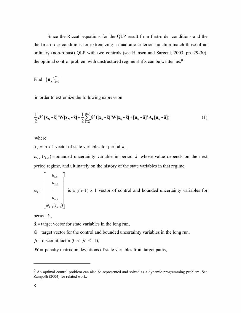
Since the Riccati equations for the QLP result from first-order conditions and the

the first-order conditions for extremizing a quadratic criterion function match those of an

ordinary (non-robust) QLP with two controls (see Hansen and Sargent, 2003, pp. 29-30),

the optimal control problem with unstructured regime shifts can be written as:9

Find ( ) 1

0

N

k

−

=ku

in order to extremize the following expression:

-1

0

1 1 [ ]' [ ])2 2

NN k

kβ β

=

+ ∑

N N k k k k k[x - x]'W[x - x] ([x - x]'W[x - x]+ u - u Λ u - u% % % % % % (1)

where

=kx n x 1 vector of state variables for period k ,

1 1( )k krω + + =bounded uncertainty variable in period k whose value depends on the next

period regime, and ultimately on the history of the state variables in that regime,

1,

2,

,

k+1 1

( )

k

k

m k

k

uu

urω +

=

ku M is a (m+1) x 1 vector of control and bounded uncertainty variables for

period k ,

=x% target vector for state variables in the long run,

=u% target vector for the control and bounded uncertainty variables in the long run,

β = discount factor (0 < β ≤ 1),

=W penalty matrix on deviations of state variables from target paths,

9 An optimal control problem can also be represented and solved as a dynamic programming problem. See Zampolli (2004) for related work.

9

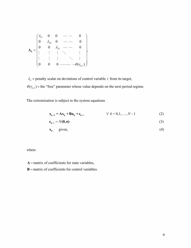
=kΛ

11

22

33

0 0 00 0 00 0 0

0 0 0

λλ

λ

θ−

L L

L L

L L

M M M O M

M M M O M

LLL 1( )kr +

,

iiλ = penalty scalar on deviations of control variable i from its target,

1( )krθ + = the “free” parameter whose value depends on the next period regime.

The extremization is subject to the system equations

1+k+1 k k kx = Ax + Bu + ε ∀ k = 0,1,.…, 1N − (2)

1 N+kε ~ (0,σ) (3)

0x given, (4)

where

=A matrix of coefficients for state variables,

=B matrix of coefficients for control variables.

10

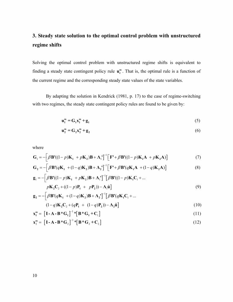
3. Steady state solution to the optimal control problem with unstructured

regime shifts

Solving the optimal control problem with unstructured regime shifts is equivalent to

finding a steady state contingent policy rule ssru . That is, the optimal rule is a function of

the current regime and the corresponding steady state values of the state variables.

By adapting the solution in Kendrick (1981, p. 17) to the case of regime-switching

with two regimes, the steady state contingent policy rules are found to be given by:

ss ss1 1 1 1u = G x + g (5)

ss ss2 2 2 2u = G x + g (6)

where

] ]

] ]

]

11 1

1

11 1

((1 ) ) ((1 ) ) (7)

( (1 ) ) ( (1 ) ) (8)

((1 ) ) ((1 )

p p p p

q q q q

p p p

β β

β β

β β

−

−

−

= − − + + + − + = − + − + + + −

= − − + + −

1 2 1 2

2 1 2 2 1 2

1 2

G B' K K B Λ ' F' B' K A K A

G B' K K B Λ ' F' B' K A K A

g B' K K B Λ ' B' K[]

] [

1

2 1

11

2

...

((1 ) )) (9)

( (1 ) ) ( ...

(1 ) ( (

p p p

q q q

q q

β β−

++ − + −

= − + − + +− + +

1

2 1 2

2 1 2 2 1

2 1

C

K C P P Λ u

g B' K K B Λ ' B' K C

K C P

%

][ ] [ ]1

1

2

1 ) )) (10)

* (11)

q−

− −

=

=

2 2

ss1 1 1

ss

P Λ u

x I - A - B*G B*G + C

x I

%

[ ] [ ]12 2 2* (12)−- A - B*G B*G + C

11

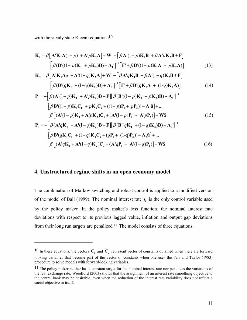
with the steady state Riccati equations10

[ ] ]] ]

[ ] ]

1

2

(1 ) (1 )

( ((1 ) ) ) ((1 ) ) (13)

(1 ) (1 )

p p p p

p p p p

q q q q

β β β

β β

β β β

−

= − + + − − + − + + + − +

= + − + − + −

1 1 2 1 2

1 2 1 1 2

1 2 1 2

K A'K A A' K A W A' K B A' K B + F

B' K K B Λ ' F' B' K A K A

K A'K A A' K A W A' K B A' K B + F

] ]

][ ]]

12

11

1

( ( (1 ) ) ) ( (1- ) ) (14)

( (1 ) ) ( ((1 ) ) )

((1 ) ((1 ) )) ...

q q q q

p p p p

p p p p

β β

β β

β

−

−

+ − + + += − − + + − + + − + + − + − +

1 2 1 2

1 2 1 2 1

1 1 2 2 1 2

B' K K B Λ ' F' B' K A K A

P A' K A' K B F B' K K B Λ '

B' K C K C P P Λ u%

]][ ]

]

1

12 2

2

( (1 ) ) ( (1 ) ) (15)

( (1 ) ) ( ( (1 ) ) )

( (1 ) ( (1-q) ))

p p p p

q q q q

q q q

β

β β

β

−

− + + − + −= − + − + + − +

+ − + + − +

1 2 1 2

1 2 1 2

1 1 2 2 1 2

A' K A' K C A' P A' P Wx

P A' K A' K B F B' K K B Λ '

B' K C K C P P Λ u

%

%

]2 1

...

( (1 ) ) ( (1 ) ) (16) q q q qβ

+ − + + − − 1 2 2A' K A' K C A' P A' P Wx%

4. Unstructured regime shifts in an open economy model

The combination of Markov switching and robust control is applied to a modified version

of the model of Ball (1999). The nominal interest rate ki is the only control variable used

by the policy maker. In the policy maker’s loss function, the nominal interest rate

deviations with respect to its previous lagged value, inflation and output gap deviations

from their long run targets are penalized.11 The model consists of three equations:

10 In these equations, the vectors 1C and 2C represent vector of constants obtained when there are forward looking variables that become part of the vector of constants when one uses the Fair and Taylor (1983) procedure to solve models with forward-looking variables. 11 The policy maker neither has a constant target for the nominal interest rate nor penalizes the variations of the real exchange rate. Woodford (2003) shows that the assignment of an interest rate smoothing objective to the central bank may be desirable, even when the reduction of the interest rate variability does not reflect a social objective in itself.

12

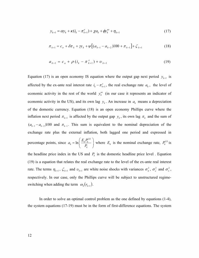
111 )( +++ +++−+= kuskk

ekkkk yaiyy ηφχπκα (17)

[ ] 11211 100)( +−−−+ ++−+++= kkkkkkk aayc ζπψγδππ π (18)

111 )( +++ +−+= kekkak ica υπρ (19)

Equation (17) is an open economy IS equation where the output gap next period 1ky + is

affected by the ex-ante real interest rate 1e

k ki π +− , the real exchange rate ka , the level of

economic activity in the rest of the world usky (in our case it represents an indicator of

economic activity in the US), and its own lag ky . An increase in ka means a depreciation

of the domestic currency. Equation (18) is an open economy Phillips curve where the

inflation next period 1kπ + is affected by the output gap ky , its own lag kπ and the sum of

1 2 1( )100 and k k ka a π− − −− . This sum is equivalent to the nominal depreciation of the

exchange rate plus the external inflation, both lagged one period and expressed in

percentage points, since lnUS

k kk

k

E PaP

=

where kE is the nominal exchange rate, US

kP is

the headline price index in the US and kP is the domestic headline price level . Equation

(19) is a equation that relates the real exchange rate to the level of the ex-ante real interest

rate. The terms 1kη + , 1kζ + and 1kυ + are white noise shocks with variances 2ησ , 2

ζσ and 2υσ ,

respectively. In our case, only the Phillips curve will be subject to unstructured regime-

switching when adding the term ( )1+kk rω .

In order to solve an optimal control problem as the one defined by equations (1-4),

the system equations (17-19) must be in the form of first-difference equations. The system

13

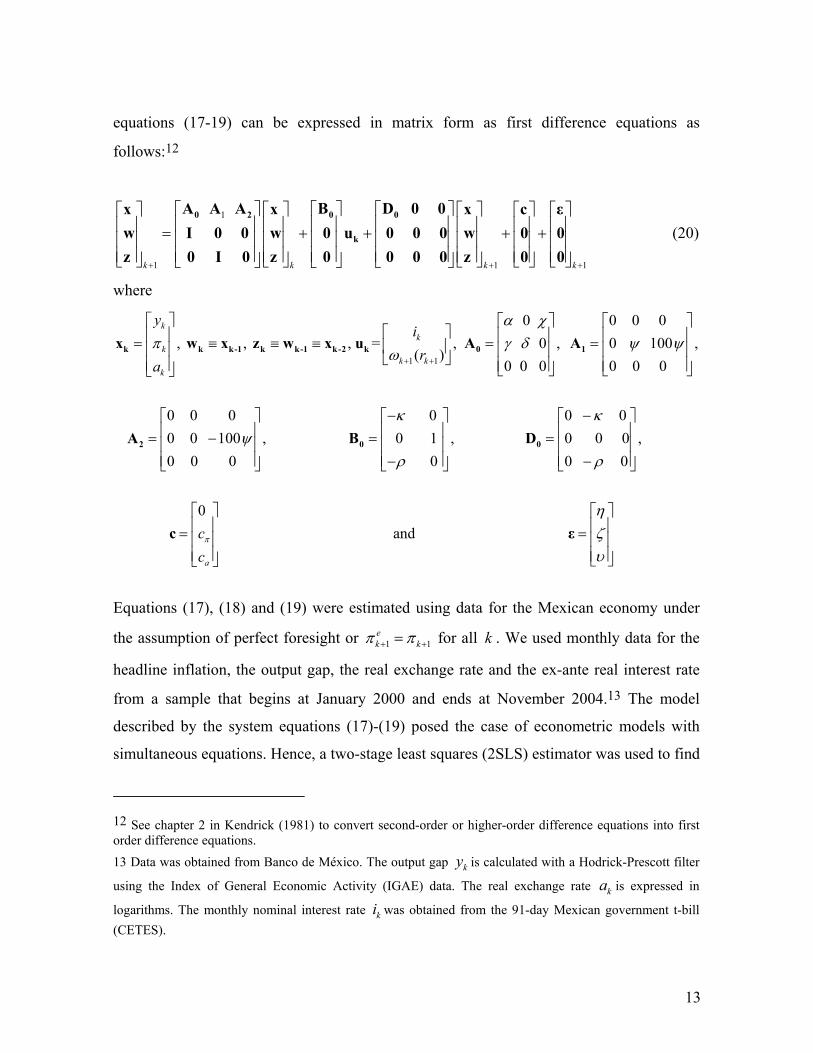
equations (17-19) can be expressed in matrix form as first difference equations as

follows:12

1

1 1 1

k k k k+ + +

= + + + +

0 2 0 0

k

A A A B D 0 0x x x c εw I 0 0 w 0 u 0 0 0 w 0 0z 0 I 0 z 0 0 0 0 z 0 0

(20)

where

1 1

0 0 0 0

, , , = , 0 , 0 100 ,( )

0 0 0 0 0 0

0 0 0 0 0 100

0

kk

kk k

k

yir

a

α χπ γ δ ψ ψ

ω

ψ

+ +

= ≡ ≡ ≡ = =

= −

k k k-1 k k-1 k-2 k 0 1

2

x w x z w x u A A

A 0 0 0

, 0 1 , 0 0 0 ,0 0 0 0 0

0

a

ccπ

κ κ

ρ ρ

− − = = − −

=

0 0B D

c and ηζυ

=

ε

Equations (17), (18) and (19) were estimated using data for the Mexican economy under

the assumption of perfect foresight or 1 1ek kπ π+ += for all k . We used monthly data for the

headline inflation, the output gap, the real exchange rate and the ex-ante real interest rate

from a sample that begins at January 2000 and ends at November 2004.13 The model

described by the system equations (17)-(19) posed the case of econometric models with

simultaneous equations. Hence, a two-stage least squares (2SLS) estimator was used to find

12 See chapter 2 in Kendrick (1981) to convert second-order or higher-order difference equations into first order difference equations. 13 Data was obtained from Banco de México. The output gap ky is calculated with a Hodrick-Prescott filter

using the Index of General Economic Activity (IGAE) data. The real exchange rate ka is expressed in

logarithms. The monthly nominal interest rate ki was obtained from the 91-day Mexican government t-bill (CETES).

14

the parameters of the model. In the first stage the parameters of Equation (18) were

estimated. In the second stage, the values of the fitted inflation replaced actual inflation in

Equations (17) and (19) and the rest of the parameters were estimated. The estimation

results and other parameter values used are shown in the Table I. The note on Table I

contains the penalty weights values used in the loss function.

Table I. Estimation results and parameter values

0.4608*** 0.9844 -0.4888*** 0.2 0.2001*** Wa

0.3985***

0.3183***

0.2597**

0.0449***

0.0153

2.9203***

-0.0583**** 5 % significance level

*** 1 % significance level

Wª is the penalty weights matrix. The penalty weights on

deviations from the inflation target are W22 = W55 = W77= 0.67.

The penalty weights on deviations from the output gap target

are W11 = W44 = W77 = 0.33 . Deviations of the real exchangerate from target do not account for any losses since the

penalty weights W33 = W66 = W99 = 0. In other words, lossesare only due to both deviations of inflation and output gapfrom their targets and those coming from interest rate firstdifferences. is the penalty weight on interest ratedeviations from its previous lagged value. The Hausman teststatistic for endogeneity was done for each equation and onlyfor the IS equation the null hypothesis was rejected.

Criterion FunctionIS Equation (GMM)

Phillips curve (OLS)

Real exchange rate equation (OLS)

α

κχ

πc

δ

acρ

γψ

χφ

β

11λ

11λ

15

5. Analysis of optimal policy responses

The optimal policy is obtained by using the solutions in Section 3 for the model described

in Section 4 represented in the matrix form given by expression (20). The discount factor

used was 0.9844. It was obtained from Schmitt-Grohe and Uribe (2001)14. The derived

optimal decision rule obtained is given by:

1 1 2, , , , , ,

ss ss ss ss ss ss ssr y r r r r a r r r r a r r a r r ri G y G G a G G a G a gπ ππ π

− − −= + + + + + + (21)

The optimal feedback rule given by Equation (21) depends on all state variables including

some lags of two of them.15 It is worth mentioning that for the problem we have described,

a simple Taylor rule is suboptimal in the sense that it only responds to inflation and output.

It is also worth noticing that the optimal feedback gains

1 1 2, , , , , ,, , , , and y r r a r r a r a rG G G G G Gπ π− − − are a function of the current regime. Now an

investigation is carried out to analyze the sensitivity of the feedback gain coefficients of

Equation (21) to changes in the magnitude of shocks and transition probabilities.

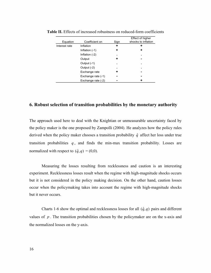
Table II summarizes the signs of the optimal feedback gain coefficients and the

effects on the magnitude of such coefficients of higher shocks to inflation.

14 Using different discount factors do not alter the main results of the paper. 15 The Phillips curve given by Equation (18) has one lag of inflation and two lags of the real exchange rate.

16

Table II. Effects of increased robustness on reduced-form coefficients

Equation Coefficient on SignEffect of higher

shocks to inflationInterest rate Inflation + +

Inflation (-1) + +Inflation (-2) . .Output + -Output (-1) . .Output (-2) . .Exchange rate + -Exchange rate (-1) - -Exchange rate (-2) - +

6. Robust selection of transition probabilities by the monetary authority

The approach used here to deal with the Knightian or unmeasurable uncertainty faced by

the policy maker is the one proposed by Zampolli (2004). He analyzes how the policy rules

derived when the policy maker chooses a transition probability q̂ affect her loss under true

transition probabilities q , and finds the min-max transition probability. Losses are

normalized with respect to ˆ( , )q q = (0,0).

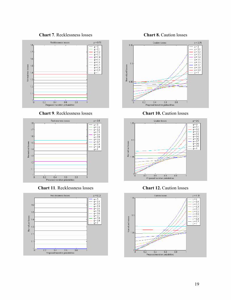
Measuring the losses resulting from recklessness and caution is an interesting

experiment. Recklessness losses result when the regime with high-magnitude shocks occurs

but it is not considered in the policy making decision. On the other hand, caution losses

occur when the policymaking takes into account the regime with high-magnitude shocks

but it never occurs.

Charts 1-6 show the optimal and recklessness losses for all ˆ( , )q q pairs and different

values of p . The transition probabilities chosen by the policymaker are on the x-axis and

the normalized losses on the y-axis.

17

As it can be seen from Charts 1, 3 and 5, the losses corresponding to low true

transition probabilities q increase as the probability chosen by the policymaker q̂

increases. On the other hand, the losses corresponding to high true probability transition

values q decrease when the chosen transition probability q̂ increases. Consequently, a

common level of the policymaker’s loss can be found. This value corresponds to the min-

max transition probability q̂ that the policymaker should select. Charts 1, 3 and 5 show

that for q̂ in the neighborhood of 0.6, the min-max probability is robust in the sense that it

delivers equal losses regardless of the true transition probability q .

Charts 2, 4 and 6 show that recklessness losses are horizontal for each q since the

policy maker ignores the possibility of switching to the regime with large price shocks.

Also, these charts show that recklessness losses increase with lower values of p --i.e.

reckless behavior is more costly when more time periods are spent in the regime

characterized by larger shocks.

Charts 8, 10 and 12 exhibit the caution losses. It can be observed that being more

prepared for the possibility of transition (choosing higher values of q̂ ) is more costly for

low true probability transition values q , if the regime with large price shocks never occurs.

Also, in Charts 7-12, it is clear that recklessness is more costly than being cautious for most

ˆ( , )q q pairs.

18

Chart 1. Optimal losses

Chart 2. Recklessness losses

Chart 3. Optimal losses

Chart 4. Recklessness losses

Chart 5. Optimal losses

Chart 6. Recklessness losses

19

Chart 7. Recklessness losses

Chart 8. Caution losses

Chart 9. Recklessness losses

Chart 10. Caution losses

Chart 11. Recklessness losses

Chart 12. Caution losses

20

The results summarized by Charts 7-12 argue in favor of caution over recklessness

in the formulation of monetary policy when there is uncertainty about the persistence of

periods with large price shocks.

Not surprisingly, both the recklessness and caution losses increase with the true

probability q . Moreover, being more cautious, as suggested by higher values of q̂ , is more

costly for lower values of q --i.e. the slope is steeper.

The shocks magnitude plays a role in selecting robust transition probabilities. The

higher the difference in magnitude, the higher the chosen probability q̂ . Charts 13 and 14

show this result. The lower value of the “free” parameter θ on Chart 14 implies a more

adverse regime with large price shocks than the one for 6.5θ = on Chart 13. Hence, the

policy maker should increase the min-max probability of switching when regime 1 is more

harmful.

Chart 13. Optimal losses for 6.5θ = Chart 14. Optimal losses for 4.6θ =

21

7. Conclusions

This paper presents an algorithm for solving an optimal control problem in which the

economy randomly alternates between two regimes characterized by different price shocks

magnitudes. The algorithm is applied to obtain the optimal monetary policy rule in an open

open economy model in which the alternation between regimes is introduced by means of

the “free” parameter commonly used when modeling unstructured uncertainty.

We find that the resulting optimal policy rule is both regime-contingent and robust.

Specifically, we find the following results: a) the optimal reaction of the interest rate is

dependent on both the actual regime and on the difference in the magnitude of shocks

between regimes; and b) after a robust selection of transition probabilities, the min-max

probability of switching to the regime with large price shocks increases when this regime is

more harmful.

For most cases, cautious behavior delivers smaller losses for the policymaker than

recklessness. Hence, these results argue in favor of caution over recklessness in the

formulation of monetary policy when there is uncertainty about the transition to a regime

characterized by large price shocks.

22

8. References

Ball, L. (1999). Policy rules for open economies. In J. Taylor (ed.), Monetary Policy Rules, pp. 127-144. The University of Chicago Press.

Blake, A.P. and Zampolli, F. (2004). Time Consistent Policy in Markov Switching Models. Manuscript, Monetary Assessment and Strategy Division, Bank of England.

Fair, R.C. and Taylor, J.B. (1983). Solution and Maximum Likelihood Estimation of Dynamic Rational Expectations Models. Econometrica 51, pp. 1169-1185.

Becker, R., Hall, S. and Rustem, B. (1994). Robust optimal decisions with stochastic nonlinear economic systems. Journal of Economic Dynamics and Control, 18, 125 147.

Giannoni, M.P. (2002). Does model uncertainty justify caution? Robust optimal monetary policy in a forward-looking model. Macroeconomic Dynamics, 6, 2002, 111–144.

Hansen, L. and Sargent, T. (2003). Robust Control and Model Uncertainty in Macroeconomics. Manuscript, www.stanford.edu/~sargent

Kendrick, D. (1981). Stochastic Control for Economic Models, 2nd ed. (2002). Mc Graw Hill, New York. Marcellino, M. and Salmon, M. (2002). Robust decision theory and the Lucas critique. Macroeconomic

Dynamics, 6, 167–185. Milani, F. (2003). Monetary Policy with a Wider Information Set: a Bayesian Model Averaging Approach.

Manuscript, http://www.princeton.edu/~fmilani/Milani (2002)_revised.pdf Onatski, A. and Stock, J.H. (2002). Robust monetary policy under model uncertainty in a small model of the

U.S. economy. Macroeconomic Dynamics, 6, 85–110. Rustem, B., Wieland, V. and Zakovic, S. (2001). A continuous min–max problem and its application to

inflation targeting. In G. Zaccour (ed.), Decision and Control in Management Science, Essays in Honor of Alan Haurie. Kluwer Academic Publishers, Boston/Dordrecht/London, pp. 201–219.

Sargent, T. (1999). Comment. In J. Taylor (ed.), Monetary Policy Rules, 144-154. The University of Chicago Press.

Schmitt-Grohe, S. and Uribe, M. (2001). Stabilization Policy and the Costs of Dollarization. Journal of Money, Credit, and Banking, Part 2, 33 (2), 482-509.

Söderström, U. (1999). Monetary Policy with Uncertain Parameters. Manuscript, Sveriges Riksbank and Stockholm School of Economics.

Stock, J.H. (1999). Comment. In J.B. Taylor (ed.), Monetary Policy Rules, 253–259. The University of Chicago Press.

Tetlow, R. and von zur Muehlen, P. (2001a). Robust monetary policy with misspecified models: Does model uncertainty always call for attenuated policy? Journal of Economic Dynamics and Control, 25, 911–949.

Tetlow, R. and von zur Muehlen, P. (2001b). Avoiding Nash Inflation: Bayesian and Robust Responses to Model Uncertainty. Working Paper, Board of Governors of the Federal Reserve System, Washington, D.C.

Walsh, C. (2004). Precautionary Policies. Federal Reserve Bank of San Francisco Economic Letter, 2004-05, February 13.

Woodford, M. (2003). Optimal Interest-Rate Smoothing. Review of Economic Studies, 70, 861-886. Zampolli, F. (2004). Optimal Monetary Policy in a Regime-Switching Economy. Manuscript, Bank of

England.