Uncertainty and Natural Resources � Prudence

facing Doomsday∗

Johannes Emmerling†

Fondazione Eni Enrico Mattei (FEEM) and CMCC

March 13, 2015

Abstract

This paper studies the optimal extraction of a non-renewable resource un-

der uncertainty using a discrete-time approach in the spirit of the literature

on precautionary savings. We �nd that boundedness of the utility function,

in particular the assumption about U(0), gives very di�erent results in the

two settings which are often considered as equivalent. For a bounded utility

function, we show that in a standard two-period setting, prudence is no longer

su�cient to ensure a more conservationist extraction policy than under cer-

tainty. If on the other hand we increase the number of periods to in�nity, we

�nd that prudence is not anymore not anymore necessary to induce a more

conservationist extraction policy and risk aversion is su�cient. These results

highlight the importance of the speci�cation of the utility function and its

behavior at the point of origin.

Keywords: Expected Utility, Non-renewable resource, Prudence, Uncertainty

JEL Classi�cation: Q30, D81

∗The author would like to thank Christian Gollier, Nicolas Treich, and François Salanié for veryhelpful comments. The usual caveat applies.†Fondazione Eni Enrico Mattei (FEEM) and CMCC, Corso Magenta, 63, 20123 Milano, Italy,

email: johannes.emmerling@feem.it

1

1 Introduction

Uncertainty is ubiquitous in the �eld of Environmental and Resource Economics.

The developments in the optimal resource extraction over time following Hotelling

(1931)1 have introduced uncertainty in this �eld starting with Kemp (1976), Loury

(1978), Gilbert (1979), and Dasgupta and Heal (1979). The size of the stock of

the resource was now assumed to be a random variable and these papers charac-

terized the optimal planned extraction path over time. Their results suggest that

uncertainty will induce a more precautionary extraction path under relatively gen-

eral conditions. Gilbert (1979) shows that for isoelastic utility and an exponential

distribution of the resource stock, extraction is initially always more conservative

than under certainty. Still these results are not very general and not always very

intuitive. For instance, Kumar (2005) showed that the optimal extraction path can

even increase over time depending on the shape of the distribution of the size of the

resource stock S. An intuition for this result is that extraction can anticipate the

resolution of uncertainty and therefore provide an incentive for faster extraction.

A more recent strand of the literature builds on decision theoretic results in the

expected utility framework, namely the precautionary savings model applying it to

the resource extraction problem. Leland (1968), Sandmo (1970), and later Kimball

(1990) studied the optimal savings decision when future income is uncertain. When

the interest rate is zero, this problem can be interpreted as the resource extraction

problem where the agent aims at optimally allocation resource consumption over

time. This isomorphism between the consumption problem and optimal resource

extraction has been exploited in detail in Lange and Treich (2008). The fundamental

result of this literature is that uncertainty induces more savings if and only if the

utility function exhibits prudence in the sense of Kimball (1990) or that its third

derivative is positive. In the context of resource depletion, this implies that prudence

is necessary and su�cient for a more conservationist extraction when facing an

uncertain resource stock.

Interestingly, these two strands of the literature obtained di�erent results with

respect to the e�ect of uncertainty on the optimal resource extraction path. The

most notable di�erence is the absence of the role of prudence in the former literature.

In this paper, we try to reconcile the results of the two di�erent approaches. We

argue that a crucial characteristic of both approaches is the assumption about the

1 In a more stylized setup, Gale (1967) coined the expression cake-eating problem for thisproblem.

2

possibility of depletion in �nite time. In the classical literature, this possibility

is explicitly allowed for since otherwise no solution to the problem exists. In the

consumption savings case on the other hand, this possibility is excluded since it is

argued that the agent would never prefer to be left with zero consumption in any

period.

The possibility of depletion is directly linked to the behavior of the utility func-

tion at zero. The classical literature on resource extraction under uncertainty needs

to impose a lower bound on U(0) as otherwise no extraction exceeding the certain

part of the resource stock will occur. In an in�nite horizon model, there will at

one point in time arrive a so-called 'moment of sorrow' (Kemp, 1976) or 'dooms-

day' (Koopmans, 1974) where consumption drops to zero. This lower bound of the

utility function has a clear economic intuition in such a partial equilibrium model.

Since substitutes of the resource are not considered, having exhausted a particular

resource is not likely to lead to the end of humanity. A backstop technology at an

arbitrarily high cost will ultimately be able to replace resource consumption thus

justifying this assumption.

In the consumption savings problem on the other hand as in Lange and Treich

(2008) or Eeckhoudt et al. (2005), the assumption U(0) = −∞ is maintained as a

su�cient condition to avoid being left with nothing in the last period. Otherwise ex-

pected utility would be minus in�nity. In the context of natural resource extraction,

however, imposing U(0) = −∞ seems questionable as discussed above. The results

can also be seen in the light of recent developments about the crucial behavior of the

utility function at zero such as Geweke (2001) or Buchholz and Schymura (2010).

In this paper we thus explicitly use a bounded from below utility function. Since

we use the expected utility model, the utility function has a cardinal interpretation

and we can without loss of generalization set the lower bound to zero (U(0) = 0).

It is important to distinguish this assumption from the more standard condition

on in�nite marginal utilita at the origin limc→0 U′(c) = +∞. The assumption of

U(0) being bounded below is actually a stronger requirement than in�nite marginal

utility at zero.

Apart from the substitutability and the behavior of the utility function at zero,

another argument for allowing exhaustion follows from the interpretation of a period

in the resource context. If one considers the duration of one period in a stylized

two period model applied to the expected time span of exhausting a non-renewable

resource stock, this suggests the duration of one period consisting in decades or

centuries rather than years making exhaustion more plausible within early periods.

3

2 A stylized model with the possibility of depletion

In this section we study a two period model of resource extraction under the as-

sumption U(0) = 0 and thus allowing for exhaustion during the �rst period. A

stock of size S which is random and is distributed according to some distribution

F (s) with support [S,∞[ is extracted and consumed over two periods. S denotes

the non-negative lower bound of S or the amount of the resource that is available

with certainty. The problem consists in maximizing the expected value of discounted

utility

VI(s1) = U(s1) + βU(S − s1) (1)

where U(st) is the standard increasing and concave utility function depending only

on st, the consumption level of the resource in period t, and we denote by β ≤ 1 the

discount factor.2

The optimal �rst-period consumption under uncertainty su1 thus can be expressed

by the �rst-order condition U ′(s1) = βE[U ′(S − s1)]. The second order condition is

automatically satis�ed if the utility function is concave. If there is no uncertainty,

and the expected value of S is available with probability one, the problem becomes

maximizing U(s1)+βU(E[S]−s1). In this case, the optimal solution under certaintysc1 must satisfy the �rst-order condition U ′(s1) = βU ′(E[S]− s1).

Comparing the two conditions it is easy to show by the Jensen inequality that

uncertainty induces a lower �rst-period consumption (su1 < sc1) for any distribution of

S if and only if U ′(s) is convex (U ′′′(st) > 0). Prudence in the sense of Kimball (1990)

is thus a necessary and su�cient condition for more conservationist extraction policy.

This important result relies on the assumption that second period consumption is

always strictly positive. One way of ensuring that depletion does not occur is by

imposing U(0) = −∞, see Lange and Treich (2008).

In the following we instead allow explicitly for the exhaustion of the resource

in the �rst period. We will refer to the model just presented as situation (I). In

situation (II), depletion in the �rst period must be explicitly accounted for. The

decision trees for both situations are shown in Figure 1. The timing of the model (II)

is as follows: The social planner announces the amount s1 planned to be extracted

and consumed during the �rst period. If the actual amount available is lower than

what was planned for period one, the resource is fully exhausted during the �rst

2This model could also be framed as stylized representation of a continuous time model wherethe actual size of the resource is learned at time T and s1 is the amount of the resource that isplanned to be extracted and consumed until that date.

4

period. Otherwise, the available amount is learned at period two and what is left is

consumed. The value function VII(s1) in situation (II) for the agent is more complex

Figure 1: The decision tree for the two models

than the one for the standard case (I). In particular, it has a kink at the endogenous

value where S = s1 and it can be written as

VII(s1) =

U(S) + βU(0) if S ≤ s1

U(s1) + βU(S − s1) if S > s1(2)

The program of maximizing expected discounted utility can now be stated as follows:

maxs1

E[U(min(S, s1)) + βU(max(S − s1, 0))] (3)

Equivalently, the program can be expressed as

maxs1

s1∫0

{U(S) + βU(0)}dF +

∞∫s1

{U(s1) + βU(S − s1)}dF (4)

First, note that the value function is continuous at S. Its �rst derivative with

respect to s1 on the other hand is continuous only if the distribution F is itself

continuous. Also, the value function is not guaranteed to be concave since the

second term in (3) contains the maximum operator. For typical utility functions

and examples we considered, however, concavity of the problem did hold.

Obviously, if s1 < S, the model is equivalent to the case (I) since exhaustion will

never appear during period one. Now we can characterize the optimal solution su1 to

program (4). In order to compute the �rst order condition, we need the assumption

U(0) = 0 since otherwise V ′II(s1) is not determined. With this assumption, the

5

�rst-order condition reads

∞∫s1

{(U ′(s1)− βU ′(S − s1)}dF = 0 (5)

which can also be written as

(1− F (s1)){U ′(s1)− βE[U ′(S − s1)|S > s1]} = 0 (6)

and looks very similar to condition of the standard case (I). The di�erence is the

conditional expectation of second-period marginal utility. What matters for the

trade-o� between �rst- and second-period consumption is the conditional expected

marginal utility only in the case where depletion does not occur during period one.

The second order condition yields

∞∫s1

{(U ′′(s1) + βU ′′(S − s1)}dF − f(s1)(U ′(s1)− βU ′(0)) < 0 (7)

and it is not necessarily satis�ed since the last term is always positive as long as

f(s1) > 0. If depletion does not occur through the �rst period, that is for s1 < S,

the value function is locally concave. For s1 → S on the other hand, it is locally

convex since the �rst term tends to zero and the second is positive, while in between

these two values it is ambiguous.

Since global concavity of the value function is not ensured in this model, we

need to verify that the optimal solution will be interior. Observe that s1 = 0 can be

excluded since it is dominated by s1 = S if β is strictly lower than one. The second

possible solution, namely s1 = S, would imply that the uncertainty is resolved

immediately while consumption in period two is zero with probability one. From

(6) it is easy to see that the �rst order condition is satis�ed at this point since

F (s1) = 1. Moreover, since we saw that the value function is convex towards the

right bound of the support of S, the point s1 = S is actually a local minimum.

This ensures that the solution will always be interior and we can restrict ourselves

to points satisfying (5). Now we can derive the fundamental result of this section:

Lemma 1. When depletion of the resource stock before the last period is possible,

prudence (U ′′′ > 0) is necessary but not su�cient to ensure a more conservationist

extraction policy under uncertainty than under certainty.

6

Proof. It would be su�cient to look at the �rst example of the following section.

Nevertheless, in order to highlight the similarities and di�erence to the standard

proofs for the role of prudence, we can compare the structure of the proofs for both

cases. If ∂VII∂s1

∣∣∣sc1

is negative, the value function reaches its maximum before sc1 and

�rst period consumption under uncertainty would be more conservationist. That is,

using the �rst order condition and substituting U ′(sc1), we need the condition

U ′(ES − sc1)− E[U ′(S − sc1)|S > sc1]!< 0 (8)

to hold. By the Jensen inequality, the left-hand side of this inequality is smaller

than U ′(ES − sc1) − U ′(E[S − sc1|S > sc1]) if and only if the agent is prudent. This

term, however is non-negative since the conditional expectation of second period's

consumption is higher or equal than the unconditional expectation. Prudence is still

necessary for a more conservationist extraction path but it is not anymore su�cient

due to the possibility of depletion in period one.

Compared to the case where running out of the resource is never possible like

in Lange and Treich (2008), we need a stronger condition for a more conservative

extraction policy when facing uncertainty. This result is somewhat surprising given

that it is intuitive that the risk of being left with nothing in the second period could

lead to an even more conservationist optimal policy.

One can get an intuition for this result from the �rst order condition (5). What

matters at the margin is only the trade-o� between �rst- and discounted second

period expected utility in the case where S is higher than �rst-period consumption

s1. For the case of depletion in period one, on the other hand, the e�ect of a marginal

increase of s1 on the increased probability of being left with nothing in period two

is exactly o�set by the higher conditional expectation E[U(S)|S < s1] in the case of

running out in the �rst period. Therefore, all that matters for the optimal decision

of s1 is the expected marginal utility in both periods only if consumption is strictly

positive. That is, the situation where doomsday arrives is disregarded. This is the

what we call the 'doomsday anyway e�ect', which counteracts the e�ect of prudence.

3 Two examples

To illustrate the implications of these results we look at three examples. First,

consider the case where S takes on the values 0 or 4 with equal probability. Here the

7

assumption of U(0) > −∞ is clearly needed since S = 0 as otherwise the problem has

no solution. Abstracting from discounting (β = 1), the optimal consumption under

certainty for any strictly concave utility function would be sc1 = 1 since E[S] = 2.

Under uncertainty however, no matter what strictly positive amount is consumed

in the �rst period, depletion occurs with the probability one half. The conditional

expected value is 4 for any strictly positive value of s1 and hence we �nd the optimal

value su1 = 2, which is larger than sc1. Here, the agent considers only the case where

there is positive consumption in both period for determining the optimal value su1 ,

that is, she considers only the optimistic case of S = 4. Importantly, this result does

only depend on the concavity of the utility function and holds independent of the

third derivative of U . Even with prudence we get unambiguously su1 > sc1 so that in

this case the doomsday anyway e�ect strictly dominates the prudence e�ect. This

shows clearly the implication of the lemma.

Secondly, consider the situation where the two equally likely values of S are 2

and 10 implying E[S] = 6 and thus sc1 = 3 (maintaining β = 1).3 Now the lower

bound S is strictly positive and the value function V u has a kink at this point. The

agent has thus to decide whether or not to run the risk of depletion during the �rst

period. Whenever su1ε[0, S], we have the classical case (I) while for a value of su1greater than the lower bound S, depletion is possible and we have case (II). Denote

the maximum on this part of the domain by suII1 and an interior maximum�if there

is one�on the interval [0, S] by suI1 . Now we have to distinguish two cases depending

on whether or not there exists an interior maximum suI1 below S.

If there is no interior maximum for some s1 lower than S, the agent always takes

the risk of being left with nothing in period two. This is the case if the agent is not

prudent (U ′′′(s) ≤ 0) or if she is prudent (U ′′′(s) > 0) but 'not too much' in the

sense that his expected utility is monotonically increasing until S. In these cases,

we have that suII1 is the global maximum of V u(s1). In our example, this implies

that suII1 = 102> sc1 = 3 and we have that �rst-period consumption is higher under

uncertainty than under certainty.

If on the other hand the agent is prudent enough such that there exists an interior

maximum suI1 < 2, the value function has two local maxima as depicted in Figure 2.

Therefore the result depends on the utility function, and in particular the degree of

prudence, and one has to compare the values of V u(s1) at the two local maxima suI1

3This can be interpreted as in Hartwick (1983) as having a certain deposit while a second oneis uncertain.

8

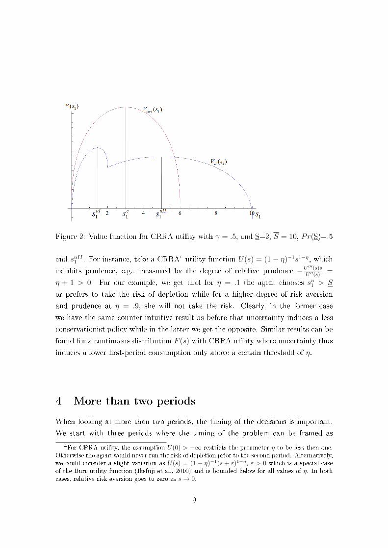
Figure 2: Value function for CRRA utility with γ = .5, and S=2, S = 10, Pr(S)=.5

and suII1 . For instance, take a CRRA4 utility function U(s) = (1− η)−1s1−η, whichexhibits prudence, e.g., measured by the degree of relative prudence −U ′′′(s)s

U ′′(s)=

η + 1 > 0. For our example, we get that for η = .1 the agent chooses su1 > S

or prefers to take the risk of depletion while for a higher degree of risk aversion

and prudence at η = .9, she will not take the risk. Clearly, in the former case

we have the same counter-intuitive result as before that uncertainty induces a less

conservationist policy while in the latter we get the opposite. Similar results can be

found for a continuous distribution F (s) with CRRA utility where uncertainty thus

induces a lower �rst-period consumption only above a certain threshold of η.

4 More than two periods

When looking at more than two periods, the timing of the decisions is important.

We start with three periods where the timing of the problem can be framed as

4For CRRA utility, the assumption U(0) > −∞ restricts the parameter η to be less then one.Otherwise the agent would never run the risk of depletion prior to the second period. Alternatively,we could consider a slight variation as U(s) = (1 − η)−1(s + ε)1−η, ε > 0 which is a special caseof the Burr utility function (Ikefuji et al., 2010) and is bounded below for all values of η. In bothcases, relative risk aversion goes to zero as s→ 0.

9

follows: at date zero, the social planner announces �rst and second period's planned

resource extraction levels whereas in the third period, what is left is extracted if

any. Moreover, if in any period the planned consumption plan cannot be realized,

the remaining amount of the resource is consumed in the same period. While one

could ask whether the planned s2 could be revised after the �rst period, it is clear

that this is never required given that the plan for the subsequent periods is already

based on the conditional expectation of the remaining resource stock for this case.

The maximization problem can be written as maximizing E[VII(s1, s2)] as

maxs1

maxs2

s1∫0

U(S)dF +

s1+s2∫s1

{U(s1) + βU(S − s1)}dF

+

∞∫s1+s2

{U(s1) + βU(s2) + β2U(S − s1 − s2)}dF

It's �rst order conditions can be written with respect to s1 as

s1+s2∫s1

{(U ′(s1)− βU ′(S − s1)}dF +

∞∫s1+s2

{(U ′(s1)− β2U ′(S − s1 − s2)}dF = 0 (9)

and with respect to s2 as

∞∫s1+s2

{(βU ′(s2)− β2U ′(S − s1 − s2)}dF = 0. (10)

The second condition is equivalent to the �rst order condition of the two-period

case. The condition with respect to �rst period's consumption on the other hand

is more complex given that a change in s1 a�ects also the second period due to the

possibility of exhaustion.

For the optimal consumption levels under uncertainty {su1 , su2} to be lower than

the levels under certainty {sc1, sc2}, we need to show that VII(s1, s2) is decreasing in

{s1, s2} at every point where the �rst order conditions under certainty are satis�ed,

that is, where the conditions U ′(s1) = βU ′(s2) = β2U ′(E[S]− s1 − s2) hold.For the second period, the condition for s2 is equivalent to the one derived in

the two-period case, namely that

su2 < sc2 ⇔ U ′(ES − s1 − s2)− E[U ′(S − s1 − s2)|S > s1 + s2] < 0. (11)

10

That is, the result from lemma 1 carries over to the second to last period. That is,

prudence is a necessary but not anymore su�cient condition for a lower consumption

level in the second period compared to the certainty case under certainty.

The case for the �rst period is more complex. For su1 to be less than the level

under certainty, sc1, we need to show that the left-hand side of (9) is negative at all

the points where the �rst-order conditions under certainty are satis�ed. Using these

conditions, we can expand the �rst term in (9) expressing it in terms of second and

third period's marginal utilities. After some reformulations, one can show that the

condition for su1 < sc1 is equivalent to

s1+s2∫s1

β{(U ′(S − s1)−U ′(s2)}dF >

∞∫s1+s2

β2{(U ′(ES − s1− s2)−U ′(S − s1− s2)}dF

(12)

The left-hand side is the di�erence in marginal utility in the second period if

depletion occurs during this period as compared to when it does not occur. This

term is always positive due to the concavity of the utility function. The term on the

right-hand side is exactly the one in the condition for second period's consumption

given by (11) which had to be negative to have su2 < sc2. Thus, the condition for

su1 < sc1 is weaker than the one for su2 < sc2.

The last result can be easily generalized for the model with more than three

periods. In this case, the respective conditions akin (12) for st for any period t =

1..T−2 include the di�erences in marginal utilities for all terms between j = t+1 and

j = T − 1 on the left hand side. Denoting by Sj the cumulative consumption until

period j, i.e., Sj ≡∑j

i=1 si, the conditions for sut < sct for any period t = 1..T − 2

can be written similar to (12) as

T−2∑j=t

Sj+1∫Sj

βj{U ′(S − Sj)− U ′(sj+1)}dF > (13)

∞∫ST−1

βT−1{U ′(E[S]− ST−1)− U ′(S − ST−1)}dF.

The summed terms on the left hand side are all non-negative. That is, the

earlier the period, the more likely is that consumption in this period is lower than

under certainty in the sense that if sut < sct holds for some period t, this is true for all

previous periods as well. For earlier periods, all periods until the last matter directly

11

for the decision on its optimal consumption. This is di�erent from the model under

certainty or the model (I) where the trade-o� shows up directly only between each

period and the last one where the realization of S is learned.

The only e�ect potentially implying a faster extraction than under certainty

comes from the second-to-last period with the interpretation we gave in the previous

section. If the right hand side of (13) is negative and we therefore have that suT−1 <

scT−1, this holds for all previous periods as well.

Finally, if we take the limit for T →∞, we obtain the discrete time equivalent of

continuous time models of resource extraction such as Kumar (2005). For a discount

factor strictly less than one, we �nally get the main result of this section.

Lemma 2. As the number of periods tends to in�nity and for a discount factor less

than one, resource consumption under uncertainty is lower for every period up to

the second-to-last period for any risk averse decision maker.

Proof. Given the discount factor β < 1, the 'doomsday anyway e�ect' of the last

period becomes nil as T → ∞. The right hand side of (13) thus becomes zero.

Since in every period j planned consumption j is higher or equal than realized

consumption, the left hand side is non- negative and strictly positive if exhaustion

occurs in �nite time. In this case, the condition (13) is satis�ed for all periods t and

resource consumption in all periods but the last two are lower under certainty than

under certainty.

As the number of periods tends to in�nity, the doomsday anyway e�ect vanishes

and the e�ect of possible exhaustion in each period dominates implying that the op-

timal extraction policy is more conservationist than under certainty if the decision

maker is risk averse. Now prudence is not anymore necessary for a more conser-

vationist policy and we obtain the classical results as in Kemp (1976) and Kumar

(2005). Contrasting this result with the two period case of the last section thus

allows to reconcile the two strands of the literatures. Depending on the assumption

about U(0), prudence is not necessary for a conservationist resource extraction pol-

icy but instead risk aversion is su�cient. A stylized two-period model on the other

hand leads to a counter-intuitive result.

5 Conclusion

While the classical literature of resource extraction under uncertainty found that

the optimal resource extraction is always more conservationist for any risk averse

12

decision maker than under certainty, the application of the qualitatively equivalent

precautionary savings model implies that this is only the case if the decision maker

is prudent (U ′′′ > 0). We show that the di�erence between the two results is a

crucial assumption about whether or not U(0) is bounded below or in other words,

whether or not exhaustion in any period is possible or not.

The results once more suggest that the discussion about the boundedness of U(0)

is important when using expected utility models in environmental economics when

considering long time horizons. This point has been discussed in recent years also

in the context of climate change and catastrophic risks, see Buchholz and Schy-

mura (2010). In the context on non-renewable resources, the substitutability of ex-

haustible resources, even at a very high cost, indicates that U(0) should be bounded

below. Applying a precautionary savings model on the other hand typically im-

poses U(0) = −∞ in order to prevent zero consumption in any period. However, it

is precisely allowing for resource consumption to drop to zero at some point (dooms-

day), which is needed in the classical resource extraction model to �nd an optimal

extraction path under uncertainty.

When we introduce this possibility in a standard two-period expected utility

framework, we �nd that prudence, while still being necessary, is no longer su�-

cient for lower �rst-period consumption than under certainty. The possibility of

exhaustion before the last period surprisingly requires stronger conditions on the

distribution and utility function to ensure a more conservationist extraction policy

than under certainty. The intuition behind this result is that the decision maker

considers for his decision about today's consumption only the case where depletion

does not occur. This 'doomsday anyway e�ect' works against the e�ect of prudence.

However, if we extend the number of periods, the condition becomes less strin-

gent the earlier the period since now in each period depletion is possible. With an

in�nite number of periods and a discount factor strictly less than one, risk aversion

is su�cient to ensure that the extraction policy will be more conservationist than

under certainty as it was found in the classical Hotelling case under uncertainty.

References

Buchholz, Wolfgang and Michael Schymura, �Expected Utility theory and the

tyranny of catastrophic risks,� Technical Report, ZEW - Zentrum für Europäische

Wirtschaftsforschung 2010.

13

Dasgupta, Partha and Geo�rey M. Heal, Economic Theory and Exhaustible

Resources, Cambridge, UK: Cambridge University Press, 1979.

Eeckhoudt, Louis, Christian Gollier, and Nicolas Treich, �Optimal consump-

tion and the timing of the resolution of uncertainty,� European Economic Review,

April 2005, 49 (3), 761�773.

Gale, David, �On Optimal Development in a Multi-Sector Economy,� Review of

Economic Studies, January 1967, 34 (1), 1�18.

Geweke, John, �A note on some limitations of CRRA utility,� Economics Letters,

June 2001, 71 (3), 341�345.

Gilbert, Richard J, �Optimal Depletion of an Uncertain Stock,� Review of Eco-

nomic Studies, January 1979, 46 (1), 47�57.

Hartwick, John M., �Learning about and Exploiting Exhaustible Resource De-

posits of Uncertain Size,� Canadian Journal of Economics, August 1983, 16 (3),

391�410.

Hotelling, Harold, �The Economics of Exhaustible Resources,� Journal of Political

Economy, April 1931, 39 (2), 137�175.

Ikefuji, Masako, Roger J. A. Laeven, J.R. Magnus, and Chris Muris, �Burr

Utility,� August 2010.

Kemp, Murray C., �How to Eat a Cake of Unknown Size (Chapter 23),� in �Three

Topics in the Theory of International Trade,� New York: American Elsevier, 1976,

pp. 297�308.

Kimball, Miles S., �Precautionary Saving in the Small and in the Large,� Econo-

metrica, January 1990, 58 (1), 53�73.

Koopmans, Tjalling C., �Proof for a Case where Discounting Advances the

Doomsday,� The Review of Economic Studies, 1974, 41, 117�120.

Kumar, Ramesh C., �How to eat a cake of unknown size: A reconsideration,�

Journal of Environmental Economics and Management, September 2005, 50 (2),

408�421.

14

Lange, Andreas and Nicolas Treich, �Uncertainty, Learning and Ambiguity in

Economic Models on Climate Policy: Some Classical Results and New Directions,�

Climatic Change, July 2008, 89 (1-2), 7�21.

Leland, Hayne E., �Saving and Uncertainty: The Precautionary Demand for Sav-

ing,� The Quarterly Journal of Economics, August 1968, 82 (3), 465�473.

Loury, Glenn C, �The Optimal Exploitation of an Unknown Reserve,� Review of

Economic Studies, October 1978, 45 (3), 621�636.

Sandmo, A., �The E�ect of Uncertainty on Saving Decisions,� The Review of Eco-

nomic Studies, July 1970, 37 (3), 353�360.

15