Embed Size (px)
Citation preview
General rights Copyright and moral rights for the publications made accessible in the public portal are retained by the authors and/or other copyright owners and it is a condition of accessing publications that users recognise and abide by the legal requirements associated with these rights.
• Users may download and print one copy of any publication from the public portal for the purpose of private study or research. • You may not further distribute the material or use it for any profit-making activity or commercial gain • You may freely distribute the URL identifying the publication in the public portal
If you believe that this document breaches copyright please contact us providing details, and we will remove access to the work immediately and investigate your claim.
Downloaded from orbit.dtu.dk on: Sep 12, 2018
Uncertainty in prediction and simulation of flow in sewer systems
Breinholt, Anders; Mikkelsen, Peter Steen; Madsen, Henrik; Grum, Morten
Publication date:2012
Document VersionPublisher's PDF, also known as Version of record
Link back to DTU Orbit
Citation (APA):Breinholt, A., Mikkelsen, P. S., Madsen, H., & Grum, M. (2012). Uncertainty in prediction and simulation of flowin sewer systems. Kgs. Lyngby: DTU Environment.

PhD ThesisMay 2012
Anders Breinholt
Uncertainty in prediction and simulation
of flow in sewer systems

Uncertainty in prediction and simulation of flow in sewer systems
Anders Breinholt
PhD Thesis May 2012
DTU Environment Department of Environmental Engineering
Technical University of Denmark

DTU Environment
May 2012
Department of Environmental Engineering
Technical University of Denmark
Miljoevej, building 113
DK-2800 Kgs. Lyngby
Denmark
+45 4525 1600
+45 4525 1610
+45 4593 2850
http://www.env.dtu.dk
Vester Kopi
Virum,
Torben Dolin
978-87-92654-60-1
Address:
Phone reception:
Phone library:
Fax:
Homepage:
E-mail:
Printed by:
Cover:
ISBN:
Anders Breinholt
Uncertainty in prediction and simulation of flow in sewer systems
PhD Thesis,
The thesis will be available as a pdf-file for downloading from the homepage of
the department: www.env.dtu.dk
May 2012
PrefaceThis PhD thesis was prepared at the Technical University of Denmark (DTU) from2007 to 2011 under the supervision of Associate Professor Peter Steen Mikkelsen(Department of Environmental Engineering, DTU Environment), Professor HenrikMadsen (Department of Informatics and Mathematical Modelling, DTU Informat-ics) and Dr. Morten Grum (Krüger A/S, a subsidiary of Veolia Water Solutions& Technologies). The PhD project was co-funded by DTU Environment, KrügerA/S and the Ministry of Science, Technology and Innovation through the graduateschool for Urban Water Technology (UWT), with supplementary financial supportfrom the Council for Strategic Research through the Storm and Wastewater Infor-matics (SWI) project.
The thesis consists of a summary report and a collection of six papers, which havebeen published or submitted to international peer reviewed journals or conferences.In the thesis the papers are referred to by their roman number, e.g. as Paper I.
Papers included in the thesis:
Paper I. Breinholt, A., Santacoloma, P.A., Mikkelsen, P.S., Madsen, H., Grum,M., Nielsen, M.K. Evaluation framework for control of integrated urban drainagesystems, In: 11ICUD, Proceedings of 11th International Conference on UrbanDrainage, Edinburgh, Scotland, 31st August-5th September 2008.
Paper II. Breinholt, A., Grum, M., Madsen, H. , Thordarson, F.Ø., Mikkelsen,P.S. Informal uncertainty analysis (GLUE) of continuous flow simulation ina hybrid sewer system with infiltration inflow - consistency of containmentratios in calibration and validation?, submitted.
Paper III. Breinholt, A., Thordarson, F.Ø., Møller, J.K., Grum, M., Mikkelsen,P.S., Madsen, H. Grey-box modelling of flow in sewer systems with state de-pendent diffusion, Environmetrics, Vol. 22 (8), pp. 946-961, 2011 (DOI:10.1002/env.1135).
Paper IV. Thordarson, F.Ø., Breinholt, A., Møller, J.K., Mikkelsen, P.S. Grum,M., Madsen, H. ,Evaluation of probabilistic flow predictions in sewer systemsusing grey box models and a skill score criterion. Stochastic EnvironmentalResearch and Risk Assessment. (in press)(DOI: 10.1007/s00477-012-0563-3).
i
Paper V. Breinholt, A., Møller, J.K., Madsen, H., Mikkelsen, P.S. A formal sta-tistical approach to representing uncertainty in rainfall-runoff modelling withfocus on residual analysis and probabilistic output evaluation - distinguishingsimulation and prediction, submitted.
Paper VI. Breinholt, A., Thordarson, F.Ø., Møller, J.K., Grum, M., Mikkelsen,P.S., Madsen, H. Identifying the appropriate physical complexity of stochasticgray-box models used for urban drainage flow prediction by evaluating theirpoint and probabilistic forecast skill, submitted.
Other publications:The following papers and reports were also prepared during the project period. Thescientific content is covered, or partly covered by the included papers. Therefore,these publications are not included in the monograph.
Breinholt, A., Grum, M., Madsen, H. , Mikkelsen, P.S. Uncertainty Analysis ofStorm- and Wastewater models, 8UDM & 2RWHM. The 8th InternationalConference on Urban Drainage Modelling. The 2nd International Conferenceon Rainwater Harvesting and Management, 7-12 September, 2009, Tokyo,Japan, Proceedings.
Hansen, L.S, Borup, M., Breinholt, A., Mikkelsen, P.S. Performance of MOUSEUPDATE for level and flow forecasting in urban drainage systems, MIKE byDHI International Conference Copenhagen 2010," Modelling in a World ofChange" 6-8 September, 2010, DHI, Hørsholm, published in proceedings/book.
Breinholt, A., Sharma, A.K. Case Area Baseline Report - Århus Public WaterUtility1, Technical Report, DTU Environment. Department of EnvironmentalEngineering. March 2010.
Breinholt, A., Sharma, A.K. Case Area Baseline Report - Copenhagen Energyand Lynette Fællesskabet2, Technical Report, DTU Environment. Departmentof Environmental Engineering. March 2010.
Breinholt, A., Sharma, A.K. Case Area Baseline Report - Avedoere WastewaterServices3, Technical Report, DTU Environment. Department of Environmen-tal Engineering. July 2009.
1http://www.swi.env.dtu.dk/upload/swi/caserapport%20%C3%A5rhus%20270310.pdf2http://www.swi.env.dtu.dk/upload/swi/casereport%20ke_lf%20270310.pdf3http://www.swi.env.dtu.dk/upload/swi/case%20area%20baseline%20report%20aved%C3%B8re%20100327.pdf
ii

The papers are not included in this www-version, but can be obtained from the Li-brary at DTU Environment: Department of Environmental Engineering TechnicalUniversity of Denmark Miljoevej, Building 113 2800 Kongens Lyngby, Denmark([email protected])
iii

iv

AcknowledgementsFirst of all I would like to thank my supervisor Associate Professor Peter SteenMikkelsen (DTU Environment) for valuable and highly appreciated support andcontribution to this thesis.
Also many thanks go to my co-supervisor Professor Henrik Madsen (DTU Infor-matics) for many significant contributions to the statistical and modelling chal-lenges and also for lending me a chair at DTU Informatics.
I would also like to thank my co-supervisor Dr. Morten Grum (Krüger A/S) forvaluable comments and contributions to many of the papers included in this thesis.
I am very grateful for the cooperation with my fellow PhD student Fannar ÖrnThordarson (DTU Informatics) who introduced me to CTSM and helped me outwith various Latex and Matlab problems and for his willingness to discuss thestatistical subjects. Also I am thankfull to Assistant Professor Jan KloppenborgMøller (DTU Informatics) for his willingness to help with CTSM and to answerquestions and discuss possible new approaches to solve the statistical and mod-elling problems that I came across during my PhD. I would also like to thank As-sociate Professor Niels Kjølstad Poulsen (DTU Informatics) for beeing willing toanswer questions regarding control theory and for setting up a model platform forcontrol of urban drainage system although it was not finalised within the project.
I am also very grateful for the data and support I received from Spildevandscen-ter Avedøre (SCA) and especially I would like to thank Jacob Nørremark for hissupport.
v

vi
SummaryModels are commonly applied for design of urban drainage systems. Typicallythey are of deterministic nature although it is well accepted that they only reflectreality approximately. When measurements are available they can be used for cal-ibration of models. However, deviations between model outputs and observationswill often remain and should hence be quantified, especially when used for modelpredictive control.
The objective with this thesis has been to quantify and qualify the modelled out-put uncertainty. For this purpose a catchment in Ballerup (1,320 hectares) wasselected and data included flow from downstream the catchment, rain measured attwo rain gauges and monthly evaporation. The data period covered subperiods of2007-2010. The catchment area consists of both combined and separated drainagesystems and significant infiltration inflow enters the system through permeable sur-face areas. The simple serial linear reservoir flow routing principle was applied formodelling both the fast rainfall runoff from paved areas and the slow infiltrationinflow from permeable areas. The wastewater flow variation was modelled by aharmonic function. Models of different complexity in terms of describing featuressuch as flow constraints, basins and pumps were tested for their ability to describethe output with a time resolution of 15 minutes.
Two approaches to uncertainty quantification were distinguished and adopted, thestochastic and the epistemic method. Stochastic uncertainty refers to the random-ness observed in nature, which is normally irreducible due to the inherent variationof physical systems. Epistemic uncertainty on the contrary arises from incom-plete knowledge about a physical system. For quantifying stochastic uncertaintiesa frequentist approach was applied whereas the generalised likelihood uncertaintyestimation method (GLUE) was adopted for the epistemic approach. Two differentuncertainty estimates were furthermore distinguished: prediction and simulationuncertainty. To quantify the prediction uncertainty the model should accommodatean updating step thereby benefitting from observations that arrive in continuationof the predictions made. The simulation uncertainty on the other hand is calculatedfrom data of a limited measuring campaign and the model does not accommodate amodel correction step. The stochastic approach was applied for uncertainty quan-tification in both prediction and simulation whereas the epistemic uncertainty wasassessed only in simulation. A maximum likelihood method was applied for pa-rameter estimation in the stochastic approach, i.e. one optimal parameter set was
vii
derived that minimises the errors between model outputs and observations. Con-versely in GLUE, parameters are viewed as stochastic variables and many accept-able parameter sets were therefore identified.
The predictive stochastic models were built on stochastic differential equations thatinclude a drift term containing the physical description of the model and a diffusionterm describing the uncertainty in the state variables. Additionally the observationnoise is accounted for by a separate observation noise term. This approach is alsoreferred to as stochastic grey-box modelling. A state dependent diffusion termwas developed using a Lamperti transformation of the states, and implemented tocompensate for heteroscedastic state uncertainty and to avoid predicting negativestates. A flow proportional observation noise term introduced by a log transformwas furthermore used to avoid predicting negative flows.
In the simplest stochastic prediction models all parameters were estimated easily;however increasing the deterministic model complexity involved that some of theparameters had to be fixed. The statistical assumptions that require the residualsto correspond to a white noise process were fulfilled for the one-step predictionbut beyond the one-step prediction auto-correlated residuals were obtained. TheAkaike’s (AIC) and the Bayesian (BIC) information criteria were used to identifypreferred models for the one-step prediction whereas a skill scoring criterion ad-dressing both the reliability and the sharpness of the confidence bounds was usedwhen assessing the forecasting performance beyond the one-step. The reliabilitywas satisfied for the one-step prediction but were increasingly biased as the pre-diction horizon was expanded, particularly in rainy periods.
GLUE was applied for estimating uncertainty in such a way that the selection ofbehavioral parameter sets continued until a required coverage of observations wasobtained (targeting 90%). A likelihood measure were used for ranking the param-eter sets and two different ways of drawing parameter sets were tested, a Latin Hy-percube Monte Carlo method and a modified Monte Carlo Markov Chain method.When using the stochastic models for simulation, it was found that the simulationuncertainty was best described when estimating parameters by the output errorminimisation method. In order to remove the heteroschedastic residuals structureit were necessary to apply a transformation of the observations, however autocorre-lation remained in the simulation case. A skill scoring comparison of a simulationand a prediction model showed that a major improvement is gained by updatingthe model states continuously, i.e. updating of model states results in much lower
viii
forecasting uncertainty at shorter prediction steps.
In the GLUE methodology there are no requirements to the residuals. Neverthelessthe aim is the same as for the stochastic simulation models, namely to cover aproportion of observations consistent with the considered quantile with maximumsharpness, i.e. to minimise the skill score. In one calibration case, even thoughvery broad prior parameter ranges were specified, it was difficult to acquire a 90%coverage of observations and the reliability in rainy periods was much lower thanin dry weather. However the GLUE method proved quite consistent in the sensethat similar coverage rates were obtained in both calibration and validation periodswith the same set of retained parameter sets.
A comparison of the stochastic and epistemic approaches to uncertainty evaluationwas conducted by comparing the sharpness, the reliability and the skill score onthe same set of data. Very similar performance was obtained with the stochasticmethod as the preferred. The thesis has demonstrated that the statistical require-ments to the formal stochastic approach are very hard to fulfill in practice whenprediction steps beyond the one-step is considered. Thus the underlying assump-tion of the GLUE methodology, that uncertainty in modeling and simulation is notonly of stochastic nature, seems fairly consistent with the results of this thesis.
A major drawback of the GLUE methodology as applied here is the lumpingof total uncertainty into the parameters, which entails a loss of physicality ofthe model parameters. Conversely the parameter estimates of the stochastic ap-proach are physically meaningful. This thesis has contributed to developing sim-plified rainfall-runoff models that are suitable for model predictive control of urbandrainage systems that takes uncertainty into account.
ix

x
Dansk sammenfatningModeller anvendes hyppigt til design af regn- og spildevandssystemer i urbaneoplande. Sådanne modeller er normalt deterministiske omend det er velkendt, atmodellerne sjældent afspejler virkeligheden perfekt. I de tilfælde hvor målingerer tilgængelige kan modellerne kalibreres. Men ofte vil der være afvigelser somignoreres, og denne usikkerhed bør reelt kvantificeres hvilket særligt gælder iforbindelse med styringer der omfatter modelprædiktioner.
Formålet med afhandlingen har således været at finde metoder til at kvantificere ogkvalificere modellernes output usikkerheder. Til dette formål blev et caseoplandbeliggende i Ballerup (1.320 ha) udvalgt, og flowdata målt nedstrøms fra oplan-det blev anvendt til modellering og usikkerhedskvantificering. Input til modellerneomfattede regn fra to regnmålere samt månedlige fordampningsdata. Den samlededataperiode udgjorde 2007-2010. Caseoplandet rummer både fælles og separatkloakerede oplande og er påvirket af uvedkommende infiltrationsvand fra perme-able områder. Det linære reservoir princip blev benyttet til modellering af reg-nafstrømning og infiltration og en harmonisk funktion beskrev spildevandsflowet.Derudover antog modellerne forskellig kompleksistet med hensyn til beskrivelsenaf flowbegrænsninger, overløb samt pumper. Modellernes output blev sammen-holdt med observationerne med en tidsopløsning på 15 minutter.
Der er skelnet mellem to overordnede tilgange til usikkerhedskvantificering, denstokastiske og den epistemiske . I den stokastiske verden opfattes usikkerhedersom tilfældige, irreducerbare og som kvantificerbare størrelser, mens usikkerhederi den epistemiske tilgang beror på utilstrækkelig viden om et givent fysisk system.Til kvantificering af usikkerheder benyttes henholdsvis en frekventistisk statistiskmetode til at repræsentere den stokastiske tilgang, og GLUE metoden (GeneralisedLikelihood Uncertainty Estimation) som repræsentant for den epistemiske tilgang.Derudover blev skelnet mellem usikkerhedsbestemmelse i simulation og prædik-tion. Hvilken type usikkerhedsbestemmelse der kan estimeres vil afhænge af omder er on-line målinger tilgængelige for løbende opdatering/korrektion af modelleneller ej. Prædiktionsusikkerheden bestemmes ved løbende opdatering mens simu-lationsusikkerheden bestemmes ud fra en afgrænset måleperiode. Den stokastiskemetode blev anvendt til bestemmelse af usikkerheden i både prædiktion og sim-ulation, mens den epistemiske kun blev anvendt til bestemmelse af usikkerhedenunder simulation. I den stokastiske metode benyttes maksimum likelihood esti-mation til at finde det optimale parametersæt dvs. til at minimere fejlen mellem
xi
modellens output og observationerne. I GLUE derimod opfattes parametersæt somstokastiske variable og mange egnede parametersæt findes.
I den stokastiske metode formuleres modellen ved hjælp af stokastiske differen-tialligninger som indeholder to vigtige led, et driftsled og et diffusionsled. Drift-sledet rummer den fysiske beskrivelse af modellen mens diffusionsledet beskriverusikkerheden i tilstandsvariablene. Derudover findes et separat usikkerhedsled derbeskriver observationsusikkerheden. Den benyttede stokastiske metode er i denneafhandling også benævnt stokastisk grey-box modellering. For at tage højde for til-standsafhængig usikkerhed blev et tilstandsafhængigt diffusionsled implementeretved hjælp af Lamperti transformation hvilket sikrede positive tilstandsvariable.Tilsvarende sikrede et flowafhængigt observationsled positive flows.
I de simple modeller kunne alle parametre estimeres, men med voksende mod-elkompleksitet blev det vanskeligere at estimere alle parametrene hvorfor nogleparametre måtte fikseres. De statistiske forudsætninger for de stokastiske modellerindebærer at residualerne skal svare til en hvid støjproces. Dette var en rimeligantagelse for et-trins prædiktionen men antagelsen var ikke opfyldt for flertrins-prædiktionen samt ved simulation pga. autokorrelerede residualled. Information-skriterierne Akaike’s (AIC) og det Bayesianske (BIC) blev benyttet til udvælgelseaf den mest velegnede model til et-trins prædiktionen, mens et interval skill scorekriterium blev anvendt til udvælgelse af den mest velegnede model til flertrinsprædiktioner samt simulation. Interval skill scoren sammenholder den faktiskeprocent af observationerne der falder indenfor et givent konfidensbånd med denforventede (reliabiliteten), og tager højde for konfidensbåndenes bredde. Relia-biliteten for konfidensbåndene viste god overenstemmelse for et-trinsprædiktionenmen reliabiliteten faldt med voksende prædiktionshorisont og var generelt dårligerei regnvejr end i tørvejr.
I GLUE metoden bestemmes usikkerheden ved udvælgelse af parametersæt indtilen passende dækning af observationer opnås (f.eks. 90%). Rangordningen af ogvalget af egnede parametersæt blev foretaget ved hjælp af et uformelt likelihoodmål, og udtrækning af parametersæt skete på to måder dels via en latin hypercubeMonte Carlo metode, og dels med en Markov Chain Monte Carlo metode.
Det viste sig at den mest optimale simulationsmodel var en model hvor den sam-lede outputfejl blev minimeret, og hvor det var nødvendigt at transformere måle-data for at fjerne de heteroskedastiske residualled. Autokorrelationen kunne dog
xii

ikke fjernes, og kan næppe fjernes i en simulationsmodel, hvorfor det statistiskegrundlag ikke var helt opfyldt. Parametrene var generelt signifikante i simula-tionsmodellerne men enkelte parametre måtte fikseres. En sammenligning af skillscoren for en simulationsmodel og en prædiktionsmodel viste, at en væsentligforbedring i prædiktionsevne opnås ved løbende opdatering af modellen.
I GLUE metoden er der ingen krav til residualerne men målet er det samme, nemligat opnå simulationsintervaller med høj reliabilitet og smalle usikkerhedsbånd. I éttilfælde viste det sig vanskeligt at opnå 90% dækning af observationerne, på trodsaf brede prior parameterintervaller. Generelt var reliabiliteten meget dårligere iregnvejr end i tørvejr. Men metoden var målt på reliabilitet forholdsvist konsistentmellem kalibrerings- og valideringsperioderne.
De to metoder blev endvidere aftestet på det samme datagrundlag med hensyn tilreliabilitet, bredde af konfidensbånd samt skill score, og gav nogenlunde sammeresultat, omend den stokastiske metode alligevel var bedre målt på skill scoren.En fordel ved den stokastiske metode er at den kan bruges til at udlede parameter-værdier.
De statistiske forudsætninger for den stokastiske metode kunne kun overholdes foret-trins prædiktionen. Under fler-trins prædiktionen og under simulation er dersignifikant autokorrelation. På dette grundlag må det konkluderes at usikkerhedenikke kun er stokastisk men at den også beror på utilstrækkelig viden sådan somtilhængerne af den epistemiske anskuelse hævder. Denne afhandling har bidragettil udvikling af simple modeller som er velegnet til brug for modelprædiktiv styringaf afløbssystemer når usikkerheden indregnes.
xiii

xiv
ContentsPreface . . . . . . . . . . . . . . . . . . . . . . . . . . . . . . . . . . . . . . i
Acknowledgements . . . . . . . . . . . . . . . . . . . . . . . . . . . . . . . v
Summary . . . . . . . . . . . . . . . . . . . . . . . . . . . . . . . . . . . . . vii
Dansk sammenfatning . . . . . . . . . . . . . . . . . . . . . . . . . . . . . xi
1 Introduction . . . . . . . . . . . . . . . . . . . . . . . . . . . . . . . . . 11.1 Modelling within urban drainage engineering . . . . . . . . . . . . . 11.2 Sources and approaches to uncertainty quantification in rainfall-runoff
modelling . . . . . . . . . . . . . . . . . . . . . . . . . . . . . . . . . 11.3 Distinguishing simulation and prediction models with focus on con-
trol . . . . . . . . . . . . . . . . . . . . . . . . . . . . . . . . . . . . 21.4 Key research aims . . . . . . . . . . . . . . . . . . . . . . . . . . . . 41.5 Outline . . . . . . . . . . . . . . . . . . . . . . . . . . . . . . . . . . 6
2 Literature review . . . . . . . . . . . . . . . . . . . . . . . . . . . . . . 92.1 Approaches to uncertainty evaluation of model outputs and parameters 92.2 Data assimilation and model complexity . . . . . . . . . . . . . . . . 112.3 Benchmarking models and their uncertainty performance . . . . . . 13
3 Case study . . . . . . . . . . . . . . . . . . . . . . . . . . . . . . . . . . 153.1 Catchment . . . . . . . . . . . . . . . . . . . . . . . . . . . . . . . . 153.2 Data . . . . . . . . . . . . . . . . . . . . . . . . . . . . . . . . . . . . 15
4 Simplistic deterministic sewer flow modelling . . . . . . . . . . . . . . 194.1 Lumped conceptual modelling of sewer flow . . . . . . . . . . . . . 194.2 Overview of simplistic models applied . . . . . . . . . . . . . . . . . 20
5 The stochastic approach to uncertainty evaluation . . . . . . . . . . . 275.1 Stochastic grey box models . . . . . . . . . . . . . . . . . . . . . . . 275.2 Maximum likelihood parameter estimation . . . . . . . . . . . . . . 285.3 Seeking an appropriate diffusion term . . . . . . . . . . . . . . . . . 295.4 Seeking an appropriate observation noise term . . . . . . . . . . . . 325.5 The transformed grey box model with transformed observations . . . 355.6 Generating predictions and uncertainty limits using stochastic grey
box models . . . . . . . . . . . . . . . . . . . . . . . . . . . . . . . . 35
xv
6 The epistemic approach to uncertainty evaluation . . . . . . . . . . . 376.1 Introducing stochastic parameters . . . . . . . . . . . . . . . . . . . 376.2 The pseudo-Bayesian approach . . . . . . . . . . . . . . . . . . . . . 376.3 Choosing a likelihood measure and the behavioral parameter sets . . 386.4 Searching the parameter space . . . . . . . . . . . . . . . . . . . . . 396.5 Generating uncertainty limits . . . . . . . . . . . . . . . . . . . . . . 40
7 Benchmarking models and uncertainty approaches . . . . . . . . . . 437.1 Residual analysis . . . . . . . . . . . . . . . . . . . . . . . . . . . . . 437.2 Probabilistic prediction and simulation measures . . . . . . . . . . . 43
7.2.1 Reliability bias . . . . . . . . . . . . . . . . . . . . . . . . . . 447.2.2 Sharpness . . . . . . . . . . . . . . . . . . . . . . . . . . . . . 44
7.3 Model performance comparison . . . . . . . . . . . . . . . . . . . . 457.3.1 Evaluation using information criteria . . . . . . . . . . . . . . 457.3.2 Evaluation using an interval skill score criterion . . . . . . . . 45
8 Results and discussion . . . . . . . . . . . . . . . . . . . . . . . . . . . 478.1 Results of the stochastic approach . . . . . . . . . . . . . . . . . . . 47
8.1.1 Checking the statistical assumptions . . . . . . . . . . . . . . . 478.1.2 Selecting among model candidates by information criteria . . 498.1.3 Evaluating prediction and simulation bounds . . . . . . . . . . 50
8.2 Results of the epistemic approach . . . . . . . . . . . . . . . . . . . 568.2.1 Extraction of behavioural parameter sets . . . . . . . . . . . . 568.2.2 Parameter uncertainty . . . . . . . . . . . . . . . . . . . . . . . 578.2.3 Consistency of the GLUE generated bounds . . . . . . . . . . 58
8.3 Comparison of the stochastic and epistemic approaches . . . . . . . 59
9 Conclusions . . . . . . . . . . . . . . . . . . . . . . . . . . . . . . . . . . 63
10 Outlook . . . . . . . . . . . . . . . . . . . . . . . . . . . . . . . . . . . . 67
11 References . . . . . . . . . . . . . . . . . . . . . . . . . . . . . . . . . . 69
12 Papers . . . . . . . . . . . . . . . . . . . . . . . . . . . . . . . . . . . . . 77
xvi

1 Introduction1.1 Modelling within urban drainage engineeringModels of urban drainage systems serve many important purposes, some of whichare listed below:
• Design of drainage systems.• Evaluation of an existing drainage systems performance by checking that the
statutory requirements are met.• Investigating upgrading or redesign proposals.• Check where flooding of basements and terrain will occur.• Investigating the consequences of climate change.• Modelling of pollution discharges.• For real-time control of pumps, gates, orifices, weirs and waste water treat-
ment plants to optimise the mututal performance.
The models applied for the listed purposes are normally deterministic models as-suming to model reality perfectly. However due to the presence of various uncer-tainties these models should not be expected to reflect reality perfectly. In this the-sis different methods to quantify output uncertainty will be addressed in the casewhen data are available for model output comparison, and rainfall-runoff (RR)modelling will serve as illustrative examples.
1.2 Sources and approaches to uncertainty quantifi-cation in rainfall-runoff modelling
Although many uncertainty typologies exist each serving a specific purpose, in thisthesis the focus is on uncertainty in model-based decision support, and uncertaintyis recognised as any departure from the ideal of complete determinism, a definitionalso adopted by Walker et al. (2005).
It is generally accepted that errors and biases (or uncertainty) in RR modellingresults from the following sources (Refsgaard et al., 2007; Renard et al., 2010;Peel and Blöschl, 2011):
1. Input uncertainty due to sampling and measurement errors and inadequatespatio-temporal rainfall variability coverage.
2. Output observation uncertainty, i.e. inaccurate flow/level measurements.
1
3. Model structural uncertainty due to incomplete understanding and simplifieddescriptions of modelled processes as compared to reality.
4. Parameter uncertainty, i.e. uncertainty related to parameter values.
A thorough account of references to each of these sources is given in Peel andBlöschl (2011). Within RR modelling many different approaches to uncertaintyevaluation exists (Matott et al., 2009) but uncertainty can be broadly classified asstochastic or epistemic. Stochastic uncertainty refers to the randomness observedin nature, which is normally irreducible due to the inherent variation of physicalsystems. Epistemic uncertainty on the contrary arises from incomplete knowledgeabout a physical system (Refsgaard et al., 2007; Fu et al., 2011; Beven et al., 2011).In this thesis both a stochastic and epistemic approach to uncertainty evaluationwill be adopted and compared.
1.3 Distinguishing simulation and prediction modelswith focus on control
In general we should distinguish models suitable for prediction from models suit-able for simulation. A model tailored for long-term simulations should describethe important long-term phenomena of the system whereas a model tailored forprediction or forecasting (referred to also as a real-time- or on-line model) ac-commodates an updating step thereby benefitting from observations that normallyarrive in immediate continuation of the predictions made. Due to this continuousupdating/correction of the model a simple model structure will often suffice forpredicting the short term (Carstensen et al., 1998; Dorado et al., 2003).
Simulation models are used for all the purposes listed in Section 1.1 while pre-diction models are relevant only in connection with real-time warning or controlsystems for urban drainage systems. Simulation models are often used to test andcompare different control strategies (in a deterministic way) but outputs gener-ated from simulation models are also normally used for model predictive control.In both cases the uncertainty of the output plays a significant role. An untappedmodel predictive control potential is identified in many sewer systems and gener-ally considered to be a cheap alternative to traditional storage solutions (Paper I),but as the model predictions are uncertain, there is a risk that a wrong decision maybe taken on the basis of the model predictions. In general predictive uncertaintycan be defined as the uncertainty that a decision maker has on the future evolution
2

of a predictand that he uses to trigger a specific decision (Beven, 2009a). The re-quirement is then to provide predictions at the lead time of interest with minimumuncertainty, and to quantify this uncertainty.
Suppose we want to switch on some storm water control strategy at the WWTP inorder to increase the hydraulic capacity if the predicted flow exceeds the currentcapacity of the WWTP. Assuming it takes 2-3 hours before the plant reaches itsmaximum hydraulic capacity, then this is our desired lead time. In sewer systemswith long response time we may find sufficient lead time inside the sewer systemby monitoring the level of a storage basin, pumping station or the flow in a largeintercepting pipe, and use this information to trigger the storm water control. How-ever, it may also well be that these measurements are insufficient for predicting thehydraulic load to the WWTP or that such measurements are unavailable in realtime, and a model then will be needed.
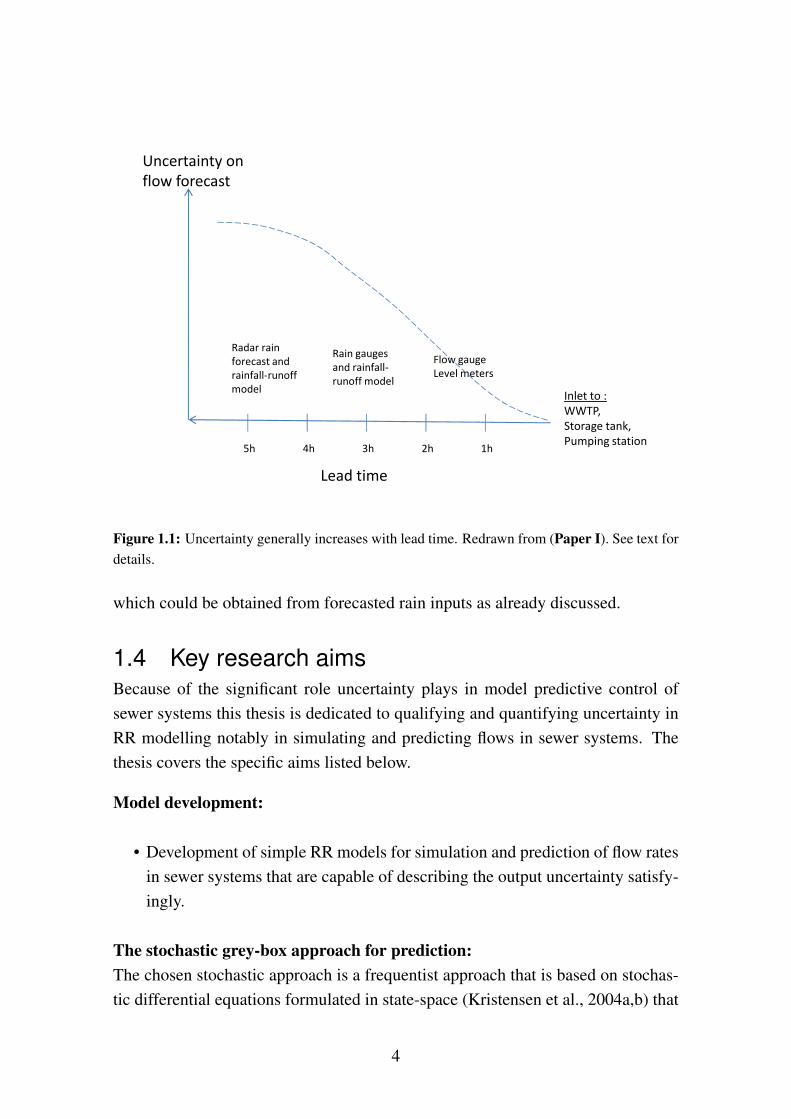
If the sewer system does not facilitate sufficient lead time because of a fast systemresponse time in the catchment (small catchment and/or steep slopes), it becomesnecessary to extend the lead time by the use of model predictions from rain gaugeinput, or if this also provides too short lead time, from forecasting the rain in-put e.g. using radars. But as indicated in Figure 1.1 increasing the lead time byforecasting the rain input normally also entails that the model predictions becomemuch more uncertain, and hence the risk that we may make a wrong decision willincrease. Achleitner et al. (2009) used radar forecasts to extend the lead time andfound uncertainty on rain volume increased up to some hundred percent for a leadtime of 3 hours. Depending on the costs of making a wrong decision we would bemore or less willing to increase the lead time and the risk of making a wrong de-cision. Considering again the WWTP control example two wrong decisions couldbe taken: (1) switching to wet weather control without the need occurring or (2)not switching to wet weather control but with the need occurring. Such a decisionshould essentially be subjected to risk analysis. In the first case the costs would beincreased outlet concentrations of nutrients and organic substances (and probablyalso increased energy costs) for a prolonged period with associated extra tax ex-penses. In the second case the WWTP would be unprepared and wastewater wouldhave to be bypassed without treatment with large impacts for the recipient. Theremay also be a model predictive control potential in optimising the utilisation ofinternal up-stream storage in the sewer system, and lead time will then be requiredfor predicting the inlet to the storage tanks or a pumping station (see Figure 1.1)
3
Uncertainty on
flow forecast
Flow gauge
Level meters
Rain gauges
and rainfall-
Radar rain
forecast and
rainfall-runoff
Inlet to :
WWTP,
Storage tank,
Pumping station1h2h3h4h5h
Level meters
Lead time
and rainfall-
runoff modelrainfall-runoff
model
Figure 1.1: Uncertainty generally increases with lead time. Redrawn from (Paper I). See text fordetails.
which could be obtained from forecasted rain inputs as already discussed.
1.4 Key research aimsBecause of the significant role uncertainty plays in model predictive control ofsewer systems this thesis is dedicated to qualifying and quantifying uncertainty inRR modelling notably in simulating and predicting flows in sewer systems. Thethesis covers the specific aims listed below.
Model development:
• Development of simple RR models for simulation and prediction of flow ratesin sewer systems that are capable of describing the output uncertainty satisfy-ingly.
The stochastic grey-box approach for prediction:The chosen stochastic approach is a frequentist approach that is based on stochas-tic differential equations formulated in state-space (Kristensen et al., 2004a,b) that
4
uses the maximum likelihood estimation method for parameter estimation. Thesystem states that contains both a drift term and a diffusion noise term is con-tinuously updated according to the measurements and the estimation method istherefore optimised to describe the one-step prediction error well. The model de-velopment involved the following steps:
• Testing of parameter significance.
• Developing suitable diffusion terms and observation noise terms.
• Checking that the actual residuals conform to the model assumed to definethe likelihood function and suggesting model improvements on the basis ofdeviations from the assumptions.
• Using statistical criteria for evaluating model performance and model com-parison.
• Testing of the model’s suitability to describe the uncertainty when the predic-tion horizon is expanded beyond the one-step ahead prediction with focus onconfidence bounds, i.e. probabilistic predictions rather than point predictions.
• Testing how the derived confidence bounds perform overall and in dry weatherand wet weather periods, respectively.
• Applying a skill scoring criterion to select the best model among severalmodel candidates when the prediction horizon is expanded beyond the firststep.
The stochastic approach for simulation:The simulation model is not continuously updated, because it is intended for longterm investigations or because data are unavailable for real time updating. Thesimulation model development involved the following steps:
• Testing of parameter significance.
• Developing suitable observation and diffusion noise terms.
• Checking that the actual residuals conform to the model assumed to definethe likelihood function and suggest model improvements on the basis of devi-ations from the assumptions.
• Testing the performance of the confidence bounds.
5
• Applying a skill scoring criterion to select the best model among several sim-ulation model candidates.
The epistemic approach to simulation:The chosen epistimic approach is based on the Generalised Likelihood Uncer-tainty Estimation (GLUE) approach (Beven and Binley, 1992). When applyingthis methodology the following items had particular focus:
• Defining a likelihood measure and a criterion for pinpointing the behaviouralparameter sets, aiming to cover a large fraction of the observations.
• Choosing a method for sampling the model space to identify the behavioralparameter sets.
• Examining the assumption that behavioural parameter sets deduced from acalibration period enables the derivation of reasonable uncertainty limits in avalidation period by checking of observation coverage.
Comparison of the stochastic and epistemic approach for simulation:The two approaches to uncertainty evaluation are finally compared and the differ-ences discussed by:
• Using a skill score criterion for comparison of the two uncertainty approacheswhen applied to the same data.
• Considering the underlying assumptions of each method.
1.5 OutlineThis summary report includes nine chapters. Following this introduction, a litter-ature review is provided in Chapter 2 that presents an overview of the uncertaintymethods commonly applied within RR modelling, some updating techniques aredescribed and the level of model complexity discussed. Finally the litterature re-view overviews some of the typical benchmarking tools applied for model compar-ison. Then the catchment and data that underlie the research is presented in Chap-ter 3. Chapter 4 gives an introduction to the simplistic modelling concept that waspursued in all the papers and also reviews the different models applied for eithersimulation or prediction in a deterministic setting. Chapter 5 outlines the stochas-tic approach to uncertainty evaluation and Chapter 6 the epistemic approach. An
6

overview of the benchmark-indicators used for prediction and uncertainty assess-ment are provided in Chapter 7 and Chapter 8 presents the results and discusses thetwo approaches to uncertainty assessment. Subsequently, the conclusions of thisthesis are drawn in Chapter 9 and some future research perspectives are outlined inChapter 10.
7

8
2 Literature reviewAssuming we are interested in realising a model predictive control potential andtherefore want to quantify the uncertainty associated with some model predictionhow should we approach that? A natural starting point is obviously to consult theliterature on this aspect.
2.1 Approaches to uncertainty evaluation of modeloutputs and parameters
As mentioned in Chapter 1 uncertainty can be broadly classified as stochastic orepistemic. These distinct interpretations of uncertainty are reflected in two majormethodologies used for uncertainty evaluation, on one hand we have the formalstatistical methods, and on the other hand we have the Generalized LikelihoodUncertainty Estimation (GLUE) methodology (Beven and Binley, 1992; Beven,2006; Beven et al., 2011). Within the formal statistical inference to uncertaintyevaluation two fundamentally different approaches to the estimation problem aredistinguished, the frequentist (or classical) approach that normally searches for asingle optimal parameter set, and the Bayesian approach that allow probabilities tobe associated with the unknown parameters (Gallagher and Doherty, 2007; Dottoet al., 2009). Another important difference is that the Bayesian approach requiresa prior distribution of the parameters whereas the frequentist approach does not.
The Bayesian approach typically involves a Markov Chain Monte Carlo (MCMC)method (Engeland et al., 2005; Yang et al., 2007; Dotto et al., 2011; Schoupsand Vrugt, 2010) with the DiffeRential Evolution Adaptive Metropolis (DREAM)scheme (Vrugt et al., 2009b,c; Vrugt, 2011) as the current state of the art for es-timating the posterior parameter distribution. Both approaches apply a likelihoodfunction that is based on formal statistical assumptions about model residuals andnormally that they correspond to a white noise process (Dotto et al., 2011; Yanget al., 2008). A comparison between a frequentist approach and a Bayesian ap-proach based on the Metropolis-Hastings algorithm showed that very similar pa-rameter uncertainty and confidence bands are found when the residuals are station-ary and ergodic (Engeland et al., 2005).
The GLUE method rejects the concept of an optimum model and parameter set,and instead acknowledges the existence of multiple likely models and parametersets (in GLUE termed equifinality). In contrast to the stochastic approach GLUEalso reject the use of statistical likelihood functions because they overestimate the
9
information content in a set of calibration data and increase the possibility of statis-tical type 1 and type 2 errors (Beven et al., 2011). Instead GLUE allows for the useof informal likelihoods (or fuzzy measures or likelihood measures) and treats resid-ual errors implicitly in making predictions. The GLUE methodology has been crit-icized for being statistically incorrect and for generating prediction limits withoutstatistical coherence (Mantovan and Todini, 2006; Mantovan et al., 2007; Stedingeret al., 2008; Vrugt et al., 2009a; Clark et al., 2011). This is due to the subjectivityin adopting a subjective likelihood measure, and in the choice of using a subjectivethreshold value to distinguish "behavioral" from "non-behavioral" parameter sets.In response hereto advocators of GLUE (Andréassian et al., 2007; Beven et al.,2007, 2008; Beven, 2009b; Beven et al., 2011) claim that the assumptions requiredfor formal statistical analysis hardly ever are satisfied within hydrological mod-elling due to epistemic errors that leads to non-stationary model-residuals that areunsuitable for statistical likelihood functions.
In most GLUE applications all the uncertainty sources outlined in Chapter 1 arelumped into the parameters and GLUE will generally give the largest parameter un-certainty compared with the stochastic approaches. Comparisons of the Bayesianand the GLUE methodology for uncertainty evaluation of outputs and parameters(Jin et al., 2010; Li et al., 2010) suggest that the two methods can, given certainrequirements to the cut-off threshold value for choosing the behavioural parame-ter sets, give more or less the same simulation output uncertainty. It is importantto recognise that a GLUE analysis can equally well be carried out using MCMCalgorithms to speed up the search for behavioural parameter sets (Blasone et al.,2008; Lindblom et al., 2011; Vezzaro and Mikkelsen, 2012), however in that caseby replacing a formal likelihood with an informal likelihood measure.
Currently research in trying to unravel the individual sources to uncertainty is on-going and the BATEA (Bayesian total error analyis) method (Kavetski et al., 2006;Thyer et al., 2007; Renard et al., 2010) is one such stochastic tool. Accordingto Renard et al. (2010) this can be useful for (1) diagnosing the main causes ofuncertainty, suggesting avenues for improving the predictive precision of RR mod-els; (2) identifying RR model deficiencies indicating opportunities for model im-provement; and (3) comparing RR models without obscuring the comparison byinput/output data errors. However, even though the method can be shown to makestatistically reliable inference and meaningfully disaggregate multiple sources ofuncertainty, in practice, if no independent estimates of data uncertainties is avail-
10
able, the discrepancy between observed and simulated responses only providesinformation about total errors. Attempts to separate uncertainty sources from oneanother has also been investigated within GLUE (Liu et al., 2009; Westerberg et al.,2010; Krueger et al., 2010).
2.2 Data assimilation and model complexityWhen using a prediction model for uncertainty quantification there is the need forcorrecting (updating) the model in real-time when a new observation is recieved.According to Refsgaard (1997) there are four variables that can be used either sep-arately or in combination for updating. These are updating in inputs or parameters,output error prediction/correction and state updating. The most common of theseare state updating and output error updating, where the error series is modelledin stochastic terms and this is used to improve the forecasts (Romanowicz et al.,2008).
A warning concerning the aim with the prediction model is issued in Beven (2009a),that decisions normally will involve the N-step ahead lead time and not just theone-step ahead prediction, the residuals of which is commonly minimised duringparameter estimation. In cases when a particular decision relies on the N-stepahead forecast, it is therefore of upmost importance to check that the derived un-certainty limits are reliable at those prediction steps and not just the one-step aheadforecast.
Within RR two main modeling philosophies can be distinguished, namely thephysically-based models (or white-box models), and the data-driven models (orblack-box models) (Todini, 2007). The physically-based models has been crit-icized for resulting in models that are overly complex, leading to problems ofoverparameterisation and equifinality, which may manifest itself in large predic-tion uncertainty. On the other hand the data-driven approach has been criticisedfor beeing too reliant on the training sets.
In the middle of this modelling spectrum a data-driven approach has been advo-cated, where complexity is added to the model only when it improves the descrip-tion of the data, without using an a priori defined model structure. The idea isto arrive at models that are complex enough to explain the data, but not morecomplex than necessary, a strategy often referred to as Occam’s razor or the prin-ciple of parsimony (Schoups et al., 2009; Todini, 2011). Such models are also re-ferred to as grey-box models (Kristensen et al., 2004a,b) or databased-mechanistic
11
Data-based
mechanistic models
Physically
based
models
MOUSE,
MOUSE,
InfoWorks,
CANOE +
Time
series KAREN,
CityDrain
BlackGreyWhite
MOUSE,
InfoWorks,
CANOE
series
models/
ANN
CityDrain
+ update/
correction
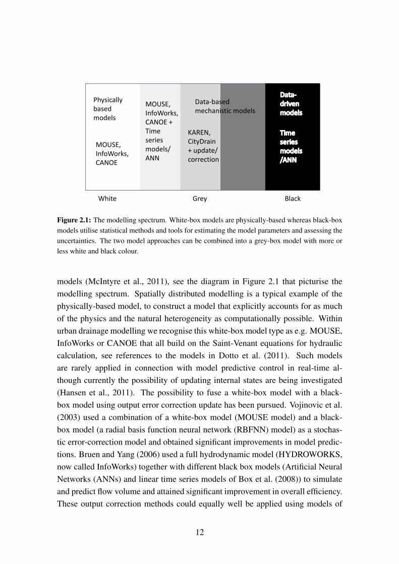
Figure 2.1: The modelling spectrum. White-box models are physically-based whereas black-boxmodels utilise statistical methods and tools for estimating the model parameters and assessing theuncertainties. The two model approaches can be combined into a grey-box model with more orless white and black colour.
models (McIntyre et al., 2011), see the diagram in Figure 2.1 that picturise themodelling spectrum. Spatially distributed modelling is a typical example of thephysically-based model, to construct a model that explicitly accounts for as muchof the physics and the natural heterogeneity as computationally possible. Withinurban drainage modelling we recognise this white-box model type as e.g. MOUSE,InfoWorks or CANOE that all build on the Saint-Venant equations for hydrauliccalculation, see references to the models in Dotto et al. (2011). Such modelsare rarely applied in connection with model predictive control in real-time al-though currently the possibility of updating internal states are being investigated(Hansen et al., 2011). The possibility to fuse a white-box model with a black-box model using output error correction update has been pursued. Vojinovic et al.(2003) used a combination of a white-box model (MOUSE model) and a black-box model (a radial basis function neural network (RBFNN) model) as a stochas-tic error-correction model and obtained significant improvements in model predic-tions. Bruen and Yang (2006) used a full hydrodynamic model (HYDROWORKS,now called InfoWorks) together with different black box models (Artificial NeuralNetworks (ANNs) and linear time series models of Box et al. (2008)) to simulateand predict flow volume and attained significant improvement in overall efficiency.These output correction methods could equally well be applied using models of
12
less complexity with simplified conceptual hydrologic flow routing methods suchas simple linear reservoirs as used in KAREN or Muskingum flow routing as usedin CityDrain (Dotto et al., 2011). Another possibility would be to update the statesof one of these more simple models using state-space filtering methods based oneither the Kalman filter (KF), the extended Kalman filter (EKF) or the ensembleKalman filter (EnKF) that updates through states and output errors. The Kalmanfilter methods demands assumptions to be made about the nature of the residualsand typically that they are Gaussian distributed, and various transformations aretherefore normally necessary to facilitate this, i.e. the Normal Quantile Transform(NQT) or Box-Cox transformations (Beven, 2009a; Coccia et al., 2011).
Todini (2011) mentions the DBM (Data Based Mechanistic Modelling) approachof (Young and Garnier, 2006; Taylor et al., 2007; Young, 2011) as a tentative at-tempt to go beyond the black-box concept by selecting among the resulting modelstructures those that are considered physically meaningful. Alternatives withoutrequirements to the residual distribution are the sequential Monte Carlo methods,also known as particle filters, that apply a Bayesian learning technique, and GLUEthat can also be applied for assessing the uncertainties in real-time forecastingby recursively updating of the behavioural parameter sets. According to (Beven,2009a) particle filters do have some limitations, they are computationally very ex-pensive and exhibit problems with estimating the posterior distribution.
2.3 Benchmarking models and their uncertainty per-formance
To benchmark models and methods within RR modelling many more or less infor-mative performance measures have been used. Deterministic model performancemeasures include the Nash & Sutcliffe efficiency coefficient (denoted E or NS)and the coefficient of determination R2 (Dotto et al., 2011), the mean square er-ror(MSE) (Achleitner et al., 2009) or root mean square error (RMSE). Accordingto Franz and Hogue (2011) much of the hydrological modeling community is stillperforming model evaluation using standard deterministic measures such as thoselisted above, and these are deficient for fully analysing model performance andshould be substituted with probabilistic assessment of model performance. Some-times model performance is supported solely by hydrograph plots of a few eventsin which typically 95% or 90% uncertainty limits are plotted together with modelobservations (Yang et al., 2007; McMillan and Clark, 2009). When uncertaintylimits or probabilistic forecasts are assessed the width (the sharpness) and the cov-
13
erage (reliability) of observations are calculated either for one or more uncertaintylimits (Renard et al., 2010; Hostache et al., 2011), and the deterministic perfor-mance measures sometimes used to assess the performance of the median (En-geland et al., 2010). The NS has also been suggested for comparing upper andlower limits among models (Laloy et al., 2010). In a GLUE study Xiong et al.(2009) introduce seven indices for characterizing the prediction bounds from dif-ferent perspectives and suggest that they be employed for assessing and comparingthe uncertainty bounds in a more comprehensive and objective way. These indicestakes the coverage, the width of the bounds and the symmetry of the bounds intoaccount.
For probabilistic performance evaluation the discrete ranked probability score, thatevaluates the squared difference between the cumulative distribution function ofthe forecast and the cumulative distribution function of a perfect forecast at somepredefined thresholds, was applied by Morawietz et al. (2011). The Brier score wasdemonstrated by Engeland et al. (2010) as an uncertainty evaluation tool for modelcomparison. The Brier score is an attractive measure for quantifying performanceof a probabilistic forecast since it combines the reliability, the resolution and themarginal distribution of a probabilistic forecast (Gneiting et al., 2007), howevermany other probabilistic evaluation methods exists (Gneiting and Raftery, 2007).
Quite commonly prediction limits or forecasting uncertainty are used in a con-text where they actually refer to simulation uncertainty. As noted by Andréassianet al. (2007) past misunderstandings on the uncertainty estimation issue wouldhave been avoided if authors had clearly defined what type of model applicationthey were discussing. That simulation and prediction models serve two differentpurposes was the subject of debate (Beven, 2009b; Vrugt et al., 2009d) followinga paper by (Vrugt et al., 2009a) in which the prediction uncertainty of a formalstatistical (Bayesian) approach was compared to the simulation uncertainty of aninformal (GLUE) approach and used to conclude that the Bayesian approach gavesmaller spread and higher coverage than the GLUE generated bounds. When mak-ing model- and/or uncertainty comparisons like these we should therefore comparelike with like, that is, simulation models with simulation models and predictionmodels with prediction models (Beven, 2009b). To avoid misunderstandings theterm "simulation uncertainty" will therefore be used when referring to uncertaintylimits or confidence bounds generated by a simulation model and "prediction un-certainty" when generated from a prediction model.
14
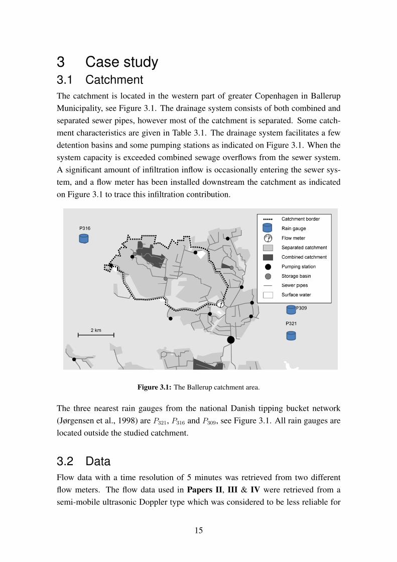
3 Case study3.1 CatchmentThe catchment is located in the western part of greater Copenhagen in BallerupMunicipality, see Figure 3.1. The drainage system consists of both combined andseparated sewer pipes, however most of the catchment is separated. Some catch-ment characteristics are given in Table 3.1. The drainage system facilitates a fewdetention basins and some pumping stations as indicated on Figure 3.1. When thesystem capacity is exceeded combined sewage overflows from the sewer system.A significant amount of infiltration inflow is occasionally entering the sewer sys-tem, and a flow meter has been installed downstream the catchment as indicatedon Figure 3.1 to trace this infiltration contribution.
P309
Figure 3.1: The Ballerup catchment area.
The three nearest rain gauges from the national Danish tipping bucket network(Jørgensen et al., 1998) are P321, P316 and P309, see Figure 3.1. All rain gauges arelocated outside the studied catchment.
3.2 DataFlow data with a time resolution of 5 minutes was retrieved from two differentflow meters. The flow data used in Papers II, III & IV were retrieved from asemi-mobile ultrasonic Doppler type which was considered to be less reliable for
15
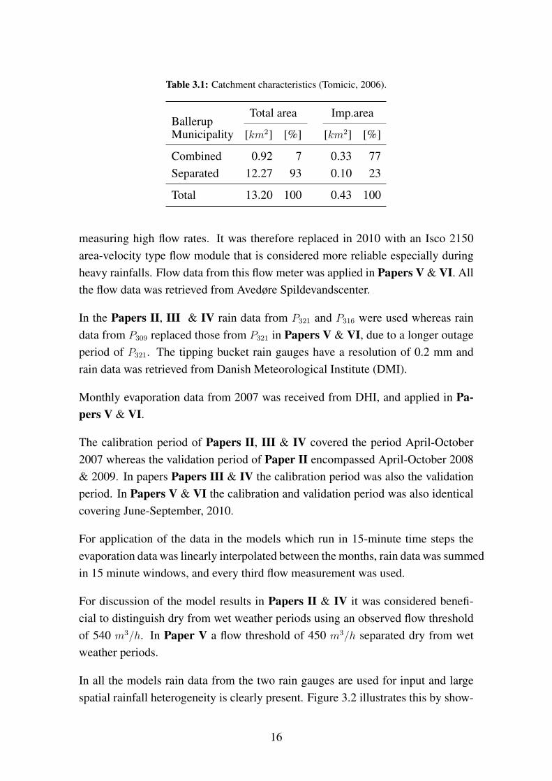
Table 3.1: Catchment characteristics (Tomicic, 2006).
BallerupTotal area Imp.area
Municipality [km2] [%] [km2] [%]
Combined 0.92 7 0.33 77Separated 12.27 93 0.10 23
Total 13.20 100 0.43 100
measuring high flow rates. It was therefore replaced in 2010 with an Isco 2150area-velocity type flow module that is considered more reliable especially duringheavy rainfalls. Flow data from this flow meter was applied in Papers V & VI. Allthe flow data was retrieved from Avedøre Spildevandscenter.
In the Papers II, III & IV rain data from P321 and P316 were used whereas raindata from P309 replaced those from P321 in Papers V & VI, due to a longer outageperiod of P321. The tipping bucket rain gauges have a resolution of 0.2 mm andrain data was retrieved from Danish Meteorological Institute (DMI).
Monthly evaporation data from 2007 was received from DHI, and applied in Pa-pers V & VI.
The calibration period of Papers II, III & IV covered the period April-October2007 whereas the validation period of Paper II encompassed April-October 2008& 2009. In papers Papers III & IV the calibration period was also the validationperiod. In Papers V & VI the calibration and validation period was also identicalcovering June-September, 2010.
For application of the data in the models which run in 15-minute time steps theevaporation data was linearly interpolated between the months, rain data was summedin 15 minute windows, and every third flow measurement was used.
For discussion of the model results in Papers II & IV it was considered benefi-cial to distinguish dry from wet weather periods using an observed flow thresholdof 540 m3/h. In Paper V a flow threshold of 450 m3/h separated dry from wetweather periods.
In all the models rain data from the two rain gauges are used for input and largespatial rainfall heterogeneity is clearly present. Figure 3.2 illustrates this by show-
16
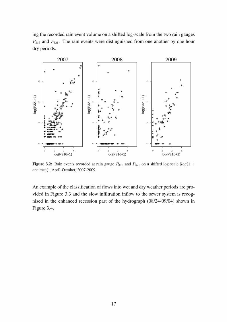
ing the recorded rain event volume on a shifted log-scale from the two rain gaugesP316 and P321. The rain events were distinguished from one another by one hourdry periods.
*
**
*
*
** **
*
*
*
*
**
**
*
*
*
*
**
**
**
*
*
*
*
**
**
*
*
*
*
*
*
*
*
*
*
***
*
*
***
*
*
*
*
***
*
*
*
**
*
*
*
*
*
**
**
*
**
**
* **
*
*
*
**
*
*
*
*
**
**
*
*
*
*
*
*
*
*
**
*
*
*
*** **
*
*
*
*
***
*
*
*
***
*
*
*
*
*
*
*
*
**
*
*
*
**
*
*
*
*
***
*
***
*
*
**
*
*
*
**
*
****
*
*
**
*
*
*
*
*
*
**
*
*
*
*
***
*
*
*
*
*
**
*
*
*
*
*
*
**
*
*
*
*
**
*
**
*
*
***
*
***
*
*
*
*
*
*
*
*
**
*
*
*
*
*
*
*
**
**
*
*
***
*
***
**
*
*
*
*
*
*
*
*
*
*
*
***
***
*
*
*
*
*
*
*
**
**
*
*
*
*
* * ** ** *0 1 2 3
01
23
log(P316+1)
log(
P32
1+1)
2007
*
*
***
**
*
*
*
*
*
*
*
**
*
*
*
*
**
***
*
*
* *
*
*
*
*
**
**
*
*
*
*
*
*
* *
*
*
** *
*
*
*
*
*
*
*
*
*
*
**
**
*
*
*
*
*
*
*
*
*
***
*
*
*
*
*
**
*
*
*
* *
**** * ** ** **** ** *** ** *** ***0 1 2 3
01
23
log(P316+1)
log(
P32
1+1)
2008
*
****
*
*
*
*
*
*
*
*
*
*
**
*
*
* *
*
*
*
*
*
*
*
*
*
*
*
*
*
*
*
*
*
*
*
*
**
**
*
*
*
*
*
*
*
****
*
*
*
*
*
* *
*
**
**
*
*
0 1 2 3
01
23
log(P316+1)
log(
P32
1+1)
2009
Figure 3.2: Rain events recorded at rain gauge P316 and P321 on a shifted log scale [log(1 +
acc.mm)], April-October, 2007-2009.
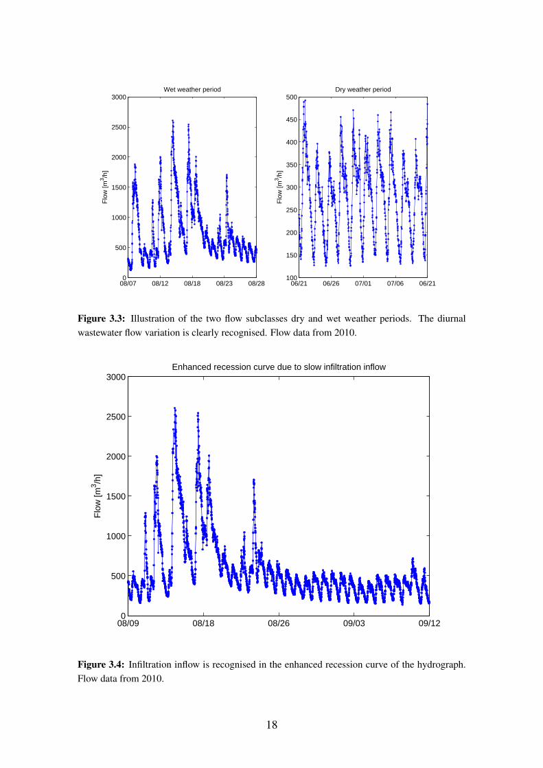
An example of the classification of flows into wet and dry weather periods are pro-vided in Figure 3.3 and the slow infiltration inflow to the sewer system is recog-nised in the enhanced recession part of the hydrograph (08/24-09/04) shown inFigure 3.4.
17
08/07 08/12 08/18 08/23 08/280
500
1000
1500
2000
2500
3000F
low
[m3 /h
]
Wet weather period
06/21 06/26 07/01 07/06 06/21100
150
200
250
300
350
400
450
500
Flo
w [m
3 /h]
Dry weather period
Figure 3.3: Illustration of the two flow subclasses dry and wet weather periods. The diurnalwastewater flow variation is clearly recognised. Flow data from 2010.
08/09 08/18 08/26 09/03 09/120
500
1000
1500
2000
2500
3000
Flo
w [m
3 /h]
Enhanced recession curve due to slow infiltration inflow
Figure 3.4: Infiltration inflow is recognised in the enhanced recession curve of the hydrograph.Flow data from 2010.
18
4 Simplistic deterministic sewer flowmodellingSince the aim with the modelling approach is to derive simple parsimonious mod-els with identifiable parameters and ability to describe the output uncertainty well,a simple modelling approach was chosen and hence the stochastic grey-box mod-elling principle is adopted. However in this Chapter the models are described deter-ministically, and in the following two chapters 5 and 6 the two distinct approachesto uncertainty evaluation will be outlined.
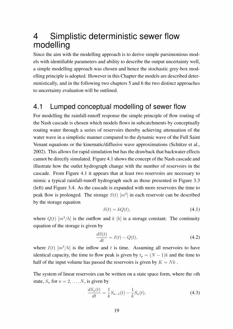
4.1 Lumped conceptual modelling of sewer flowFor modelling the rainfall-runoff response the simple principle of flow routing ofthe Nash cascade is chosen which models flows in subcatchments by conceptuallyrouting water through a series of reservoirs thereby achieving attenuation of thewater wave in a simplistic manner compared to the dynamic wave of the Full SaintVenant equations or the kinematic/diffusive wave approximations (Schütze et al.,2002). This allows for rapid simulation but has the drawback that backwater effectscannot be directly simulated. Figure 4.1 shows the concept of the Nash cascade andillustrate how the outlet hydrograph change with the number of reservoirs in thecascade. From Figure 4.1 it appears that at least two reservoirs are necessary tomimic a typical rainfall-runoff hydrograph such as those presented in Figure 3.3(left) and Figure 3.4. As the cascade is expanded with more reservoirs the time topeak flow is prolonged. The storage S(t) [m3] in each reservoir can be describedby the storage equation
S(t) = kQ(t), (4.1)
where Q(t) [m3/h] is the outflow and k [h] is a storage constant. The continuityequation of the storage is given by
dS(t)
dt= I(t)−Q(t), (4.2)
where I(t) [m3/h] is the inflow and t is time. Assuming all reservoirs to haveidentical capacity, the time to flow peak is given by tp = (N − 1)k and the time tohalf of the input volume has passed the reservoirs is given by K = Nk .
The system of linear reservoirs can be written on a state space form, where the nthstate, Sn for n = 2, . . . , N , is given by
dSn(t)
dt=
1
kSn−1(t)−
1
kSn(t), (4.3)
19
Q1(t)
Q1(t)
Q2(t)
Q (t)3
QN−1(t)
QN(t)
QN(t)
Q3(t)
Q2(t)t
t
t
t
1
2
3
N
I(t)
R E
S E
R V
O I
R S
H Y
D R
O G
R A
P H
Figure 4.1: A cascade of N linear reservoirs and the corresponding hydrographs shown to theright. Figure from Thordarson (2012).
and 4.3 can then be generalised to describe the storage in N linear reservoirs
d
dt
S1(t)S2(t)
...SN (t)
=
−NK
0 · · · 0NK
−NK
.... . .
. . .0 N
K−N
K
S1(t)S2(t)
...SN (t)
+
10...0
I(t). (4.4)
The wastewater flow variation Dt was described by a harmonic function reflectingthe diurnal pattern of water discharge from households
Dt =
2∑i=1
(si sin
i2πt
L+ ci cos
i2πt
L
), (4.5)
where L is the period of 24 hours, the parameters s1, c1, s2 and c2 are non-physicalparameters and t is time. To fully account for the wastewater flow a constant aver-age flow a0 [m
3/h] is added to Dt.
4.2 Overview of simplistic models appliedIn all models the wastewater flow was described by (4.5). Statistical tests showedthat two sinus and cosinus constants were optimal.
Conceptual model applied in Paper IIIn Paper II a model suitable for simulation was developed and hence both fast
20
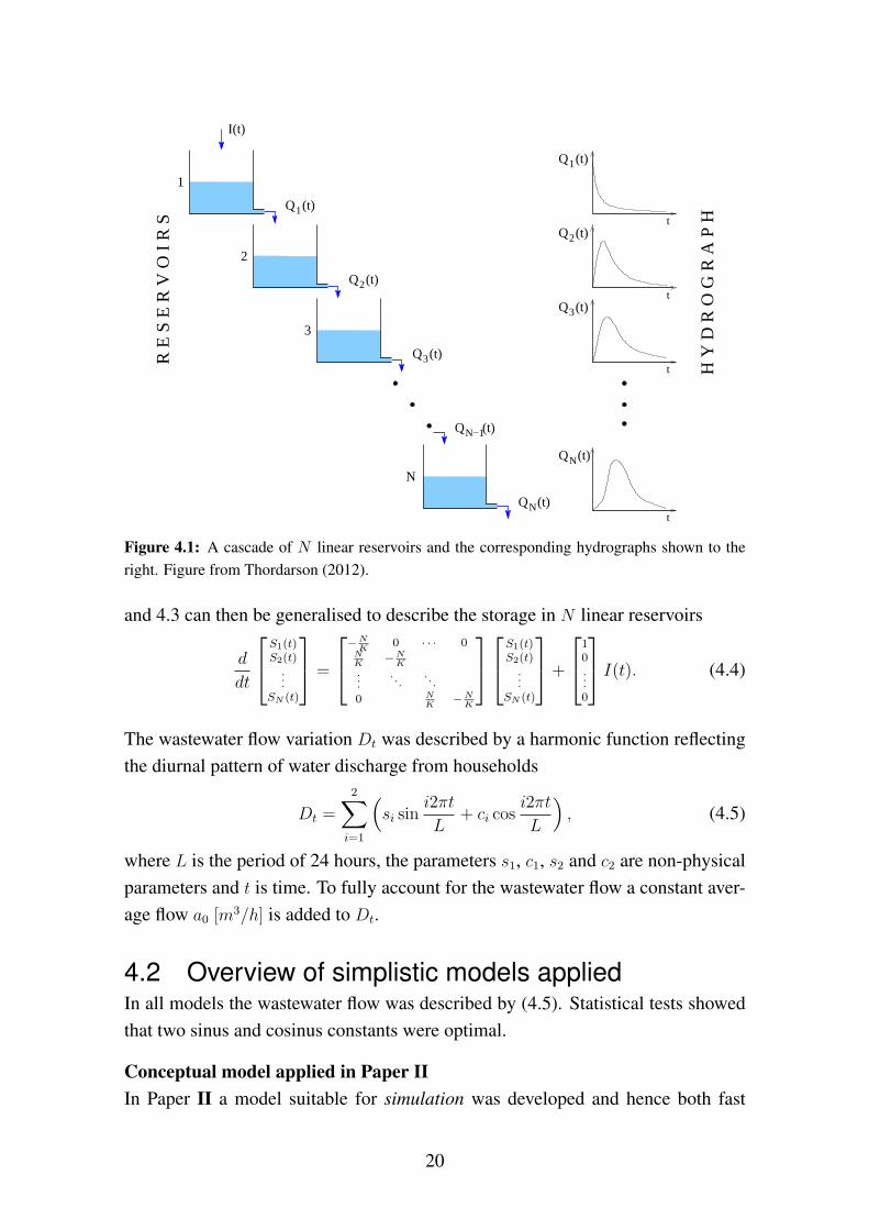
and slow runoff components were considered. The conceptual model (Figure 4.2)consists of two linear reservoirs for modelling the fast runoff (Sf1, Sf2) from pavedareas and three linear reservoirs (Ss1, Ss2, Ss3) for modelling the slow infiltration in-flow from permeable areas. Comparing the observed hydrographs of Figure 3.4 and
Figure 4.2: Graphical representation of the conceptual model used in paper Paper II.
Figure 3.3 (left) with the hydrographs in Figure 4.1 it appears that two reservoirsare sufficient for modelling the fast response because the observed hydrographs hasa rather steep rising limb. The slow infiltration inflow is expected to have a moreslow rising limb and a system of three reservoirs were therefore assumed adequate.Hence the model can be written on a state space form accordingly with (4.4):
Rainfall-runoff from paved areas
d
[Sf1,t
Sf2,t
]=
[αAfP316,t + (1− α)AfP321,t + a0 − 2
KfSf1,t
2Kf
Sf1,t − 2Kf
Sf2,t
]dt, (4.6)
where Af [ha] is the impervious fast runoff area, Kf [h] is the retention time of thefast runoff, α [−] is a rain gauge weighting coefficient, and P316 & P321 are the raingauge inputs [m/h].
21
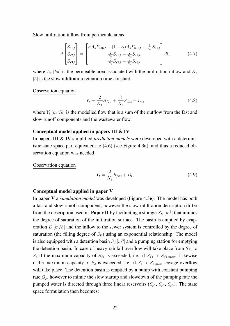
Slow infiltration inflow from permeable areas
d
Ss1,t
Ss2,t
Ss3,t
=
αAsP316,t + (1− α)AsP321,t − 2Ks
Ss1,t
2Ks
Ss1,t − 2Ks
Ss2,t
2Ks
Ss2,t − 2Ks
Ss3,t
dt, (4.7)
where As [ha] is the permeable area associated with the infiltration inflow and Ks
[h] is the slow infiltration retention time constant.
Observation equation
Yt =2
Kf
Sf2,t +3
Ks
Ss3,t +Dt, (4.8)
where Yt [m3/h] is the modelled flow that is a sum of the outflow from the fast and
slow runoff components and the wastewater flow.
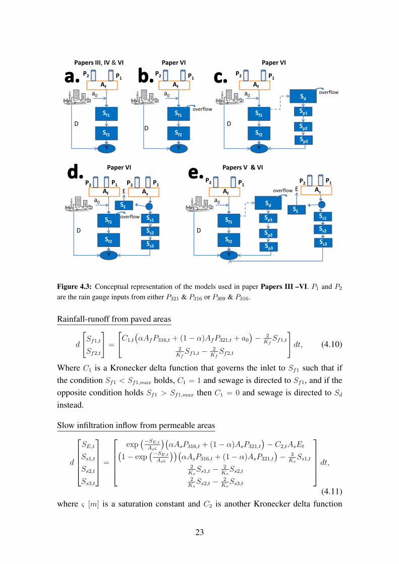
Conceptual model applied in papers III & IVIn papers III & IV simplified prediction models were developed with a determin-istic state space part equivalent to (4.6) (see Figure 4.3a), and thus a reduced ob-servation equation was needed
Observation equation
Yt =2
Kf
Sf2,t +Dt, (4.9)
Conceptual model applied in paper VIn paper V a simulation model was developed (Figure 4.3e). The model has botha fast and slow runoff component, however the slow infiltration description differfrom the description used in Paper II by facilitating a storage SE [m3] that mimicsthe degree of saturation of the infiltration surface. The basin is emptied by evap-oration E [m/h] and the inflow to the sewer system is controlled by the degree ofsaturation (the filling degree of SE) using an exponential relationship. The modelis also equipped with a detention basin Sd [m
3] and a pumping station for emptyingthe detention basin. In case of heavy rainfall overflow will take place from Sf1 toSd if the maximum capacity of Sf1 is exceeded, i.e. if Sf1 > Sf1,max. Likewiseif the maximum capacity of Sd is exceeded, i.e. if Sd > Sd,max sewage overflowwill take place. The detention basin is emptied by a pump with constant pumpingrate Qp, however to mimic the slow startup and slowdown of the pumping rate thepumped water is directed through three linear reservoirs (Sp1, Sp2, Sp3). The statespace formulation then becomes:
22
Af
a0
Sf1
Sf2
P1P2
D
Y
Papers III, IV & VI
Af
a0
Sf1
Sf2
P1P2
D
Y
Paper VI
Sd
Sp3
Sp1
Sp2
Sp3
Af
a0
Sf1
Sf2
P1P2
overflow
D
Y
Paper VI
overflow
Af
a0
Sf1
Sf2
P1P2
D
Y
As
Ss1
Ss2
Ss3
SE
P1P2
Af
a0
Sf1
Sf2
P1P2
D
Y
Sd
Sp3
Sp1
Sp2
Sp3
As
Ss1
Ss2
Ss3
SE
P1P2
E E
Paper VI Papers V & VI
overflow
overflow
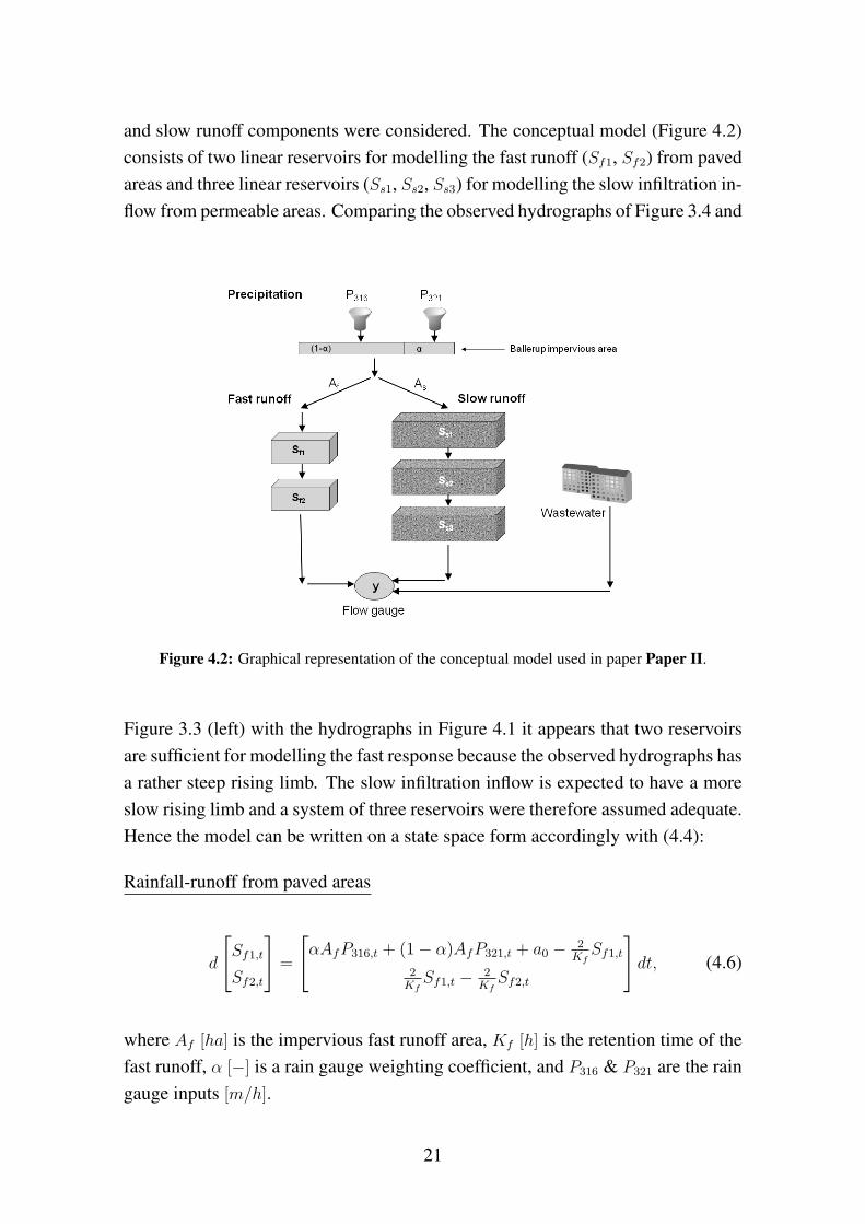
Figure 4.3: Conceptual representation of the models used in paper Papers III –VI. P1 and P2
are the rain gauge inputs from either P321 & P316 or P309 & P316.
Rainfall-runoff from paved areas
d
[Sf1,t
Sf2,t
]=
[C1,t
(αAfP316,t + (1− α)AfP321,t + a0
)− 2
KfSf1,t
2Kf
Sf1,t − 2Kf
Sf2,t
]dt, (4.10)
Where C1 is a Kronecker delta function that governs the inlet to Sf1 such that ifthe condition Sf1 < Sf1,max holds, C1 = 1 and sewage is directed to Sf1, and if theopposite condition holds Sf1 > Sf1,max then C1 = 0 and sewage is directed to Sd
instead.
Slow infiltration inflow from permeable areas
d
SE,t
Ss1,t
Ss2,t
Ss3,t
=
exp(−SE,t
Asς
)(αAsP316,t + (1− α)AsP321,t
)− C2,tAsEt(
1− exp(−SE,t
Asς
))(αAsP316,t + (1− α)AsP321,t
)− 3
KsSs1,t
2Ks
Ss1,t − 2Ks
Ss2,t
2Ks
Ss2,t − 2Ks
Ss3,t
dt,
(4.11)where ς [m] is a saturation constant and C2 is another Kronecker delta function
23
that secures a positive volume in SE by assuming the value 1 when the conditionSE > SEmin is satisfied and zero when the opposite holds.
Detention basin and pumping station
d
Sd,t
Sp1,t
Sp2,t
Sp3,t
=
(1− C1,t
)(AfP316,t + (1− α)AfP321,t + a0
)− C3,tC4,tQp,t −Qof,t
C3,tC4,tQp,t − 3Kp
Sp1,t
3Kp
Sp1,t − 3Kp
Sp2,t
3Kp
Sp2,t − 3Kp
Sp3,t
dt,
(4.12)where Qof,t = C5,t
(Sd,t−Sd,max)
dtis the overflow from the detention basin when the
maximum volume of the detention basin Sd,max is exceeded, and C5 is zero whenthe condition Sd < Sd,max is true, otherwise one. The initiation of the pump requireC3 and C4 to take the value one. C3 is one if Sd > Sd,min otherwise zero, whereSd,min is the minimum volume of the detention basin. C4 is one when Sf1 <
γSf1,max otherwise zero which secures that the pump is activated after the rain haspassed.
Observation equation
Yt =2
Kf
Sf2,t +3
Ks
Ss3,t +3
Kp
Sp3,t +Dt, (4.13)
The observation equation is extended with the outlet from the pumping station.
Conceptual models applied in paper VIIn paper VI all the models of Figure 4.3 a-e) with various physical content incor-porated (from Figure 4.3 a-e) were used for prediction.
The state space formulation of the model in Figure 4.3a is equivalent to (4.6) andthe observation equation to (4.9). The only extension of the model shown in Figure4.3b compared to Figure 4.3a is the overflow possibility in Sf1 and this implemen-tation changes the state space formulation to (4.10).
In Figure 4.3c the model is further extended with a detention basin and a pumpingstation and the overflow is now directed to the detention basin and the observationequation becomes:
Observation equation
Yt =2
Kf
Sf2,t +3
Kp
Sp3,t +Dt. (4.14)
24

In Figure 4.3d the model is equipped with the infiltration inflow description de-scribed for paper V and formulated in (4.11) and once again the fast runoff isgiven by (4.10) and the observation equation by (4.8). The last model shown inFigure 4.3e is already outlined (used in paper V).
25

26
5 The stochastic approach to uncertaintyevaluationThe stochastic approach that was chosen for this thesis is a frequentist approachthat is based on an Extended Kalman Filter (EKF) and a maximum likelihoodfunction for parameter estimation. The models are formulated in state-space anduncertainty is accounted for in the states and in the output. How this works isexplained in the following.
5.1 Stochastic grey box modelsThe deterministic models introduced in Chapter 4 can be formulated using a gen-eral notation
dXt = f(Xt,Ut, t,θ)dt (5.1)
Yk = g(Xk,Uk, tk,θ), (5.2)
where (5.1) is the system equation, describing the evolution of the states in contin-uous time and the function f(·) ∈ Rn corresponds to the deterministic state spaceformulations of the simple models introduced in Chapter 4, and (5.2) is the obser-vation equation that relates the observations to the states in discrete time by thefunction g(·) ∈ Rl consistent with the observation equations introduced in Chapter4. The time t ∈ RO indicates the continuous time and k (k = 1, . . . , K) are thediscretely observed sampling instants for K number of measurements. Y ∈ Rl is avector of output variables, X ∈ Rn a vector of state variables, θ ∈ Rp contains theunknown parameters of the system and Ut ∈ Rm is a vector of input variables.
To address uncertainties in the system the model consisting of (5.1) and (5.2) isextended with a diffusion term and an observation noise term as follows
dXt = f(Xt,Ut, t,θ)︸ ︷︷ ︸drift term
dt+ σ(Xt,Ut, t,θ)︸ ︷︷ ︸diffusion term
dωt (5.3)
Yk = g(Xk,Uk, tk,θ) + ek︸︷︷︸obs. noise term
, (5.4)
where (5.3) again is the system equation and (5.4) the observation equation. f(·)is denoted the drift term and σ(·) ∈ Rn×n is denoted the diffusion noise term orthe process noise function which represents the uncertainty of the states in thesystem, and ωt is an n-dimensional standard Wiener process, which simply meansthat the errors between the predicted states and the indirectly observed states are
27
assumed to be Gaussian distributed. The measurement error ek is assumed to bean l-dimensional white noise process with ek ∈ N (0,S(Uk, tk,θ)). The systemformulation of (5.3) and (5.4) is sometimes referred to as a stochastic grey boxmodel due to the coupling of system knowledge (from white box models) andinformation from data (black box models) that are jointly utilised for estimationof the parameters.
5.2 Maximum likelihood parameter estimationTo estimate the parameters given N number of measurements [y0,y1, . . . ,yk, . . . ,yN ],and by introducing the notation Yk = [yk,yk−1, . . . ,y1,y0], the likelihood functionis expressed as a product of conditional densities
L (θ;YN) = P (YN |θ) =
(N∏k=1
P (yk|Yk−1,θ)
)P (y0|θ) , (5.5)
where Bayes theorem P (A ∩ B) = P (A|B)P (B) is repeatedly used at each timestep to formulate the likelihood function as a product of the one step ahead condi-tional densities and where P (y0|θ) is a parameterisation of the starting conditions.It is assumed that the system equations are driven by a Wiener process which haveGaussian increments and thus the conditional probabilities in (5.5) can be approx-imated by Gaussian densities.
The Gaussian density is completely characterised by its mean and covariance of theone step prediction, which are denoted by yk|k−1 = E{yk|Yk−1,θ} and Rk|k−1 =
V {yk|Yk−1,θ}, respectively, and, by introducing an expression for the innovationformula, εk = yk − yk|k−1 the likelihood function can be rewritten as (Madsen,2008)
L (θ;YN) =
N∏k=1
exp(−1
2ε⊤k R
−1k|k−1εk
)√
det(Rk|k−1)(√
2π)lP (y0|θ), (5.6)
where the conditional mean and covariance are calculated using an EKF. The con-ditional likelihood function (5.6) minimises the one step prediction uncertainty andhence the estimation is optimised for making predictions. In the simulation casethere is no new information for conditioning as this information is not availableduring simulation. For a given set of calibration data this changes the likelihoodfunction to minimise the output error for the whole considered period
L (θ;YN) =1
(√2πS)N
exp
[ N∑k=1
1
2S(yk − yk)
2
]. (5.7)
28
The parameter estimates can be obtained by conditioning on the initial values andsolving the optimisation problem
θ = argmaxθ∈Θ
{log (L(θ;YN |y0))}. (5.8)
Numerical methods are needed to optimise the likelihood function (Kristensen andMadsen, 2003).
The maximum likelihood method also provides an assessment of the uncertaintyfor the parameter estimates in (5.8) since the maximum likelihood estimator isasymptotically normal distributed with mean θ and covariance matrix
Σθ = H−1.
The matrix H is the Fisher Information Matrix (Madsen and Thyregod, 2011)given by
hij = −E
{∂2
∂θi∂θjlog(L(θ|Yk−1))
}i, j = 1, . . . , p. (5.9)
In practice an approximation for H is obtained by the observed Hessian hij evalu-ated for θ = θ. Due to the asymptotic Gaussianity of the estimator in (5.8), a t-testcan be performed to check if the estimated parameters are statistically significant(Madsen and Thyregod, 2011).
To solve the estimation problem the open source software CTSM1 is used (Kris-tensen and Madsen, 2003; Kristensen et al., 2004a,b). The program was developedat the department of Informatics and Mathematical Modelling (IMM) at the Tech-nical University of Denmark (DTU). CTSM is capable of estimating parameters inboth linear and non-linear models using respectively an ordinary Kalman filter forlinear models and an extended kalman filter for non-linear models.
5.3 Seeking an appropriate diffusion termAs can be seen from (5.3) the diffusion term can be a function of the states, theinputs, the time, and the parameters. One may readily expect the uncertainty ofthe states to be somehow related to the rain input and more or less constant in dryweather periods suggesting the following diffusion term to apply
σ(·) =[σdry + σwet(P1,t + P2,t)
], (5.10)
where σdry represents the dry weather state uncertainty and σwet represents theadded rain proportional uncertainty in rainy periods. The rain dependent diffusion
1Continuous-Time Stochastic Modelling - www.imm.dtu.dk/ctsm
29
term was tested in combination with the drift term of (4.6) but was however foundunsuitable for two reasons. Firstly because of the time delay between a rainfall isrecorded to a state impact is observed (this time delay would be different for everyreservoir), and secondly because rapidly changing precipitation is frequently ob-served during rain, especially during convective rainfall events, whereas the stateswould exhibit much more damped changes due to the equalisation of the runofffrom a large catchment. To overcome these problems different time lags and meanprecipitation values were tested in CTSM (the mean precipitation of the last halfhour, three quarters, 1 hour) and also various low pass filters of the rain data usingthe following threshold function
Plp =Pmax
1 + exp(b0 − b1(P1 + P2)), (5.11)
where Plp is the low pass filtered rain input, Pmax the maximum rain input and b0
and b1 are threshold parameters. However, none of these proposals turned out en-tirely satisfying for describing the one step state prediction uncertainty, either itwas impossible to estimate the parameters or the residuals of the one-step predic-tion did not assume a white noise process.
Instead in Paper III different state-dependent diffusion terms were tested in com-bination with (4.6) using a state exponentiated diffusion term
σ(·) =[σiX
γii,t
], (5.12)
where σγii represents the standard deviation of the one step state uncertainty that is
scaled with the reservoir volume Xi. A state proportional uncertainty (γi=1) wasshown to best and adequately describe the one step prediction uncertainty. Theadvantage of using a state-dependent diffusion term is not just related to a betterconnection between rain input and state uncertainty, that is implicitly accountedfor by a state dependent diffusion term, but furthermore due to the natural physicalrestrictions of the system. The state variables in the models correspond to thestored volume of water in the reservoirs and obviously these have a lower limit ofzero since the water volume cannot turn negative. This lower restriction impliesthat the diffusion of the states must approach zero as the water volume in the driftterm approaches this lower boundary of zero and the state proportional diffusionterm ensures this. The state proportional diffusion term was also applied in PaperV in combination with the drift term of the states Sf2 in (4.10), Ss3 in (4.11), andSp3 in (4.12). In Paper VI different models was tested and the state proportionaldiffusion term was added to various drift terms (see Paper VI for details).
30
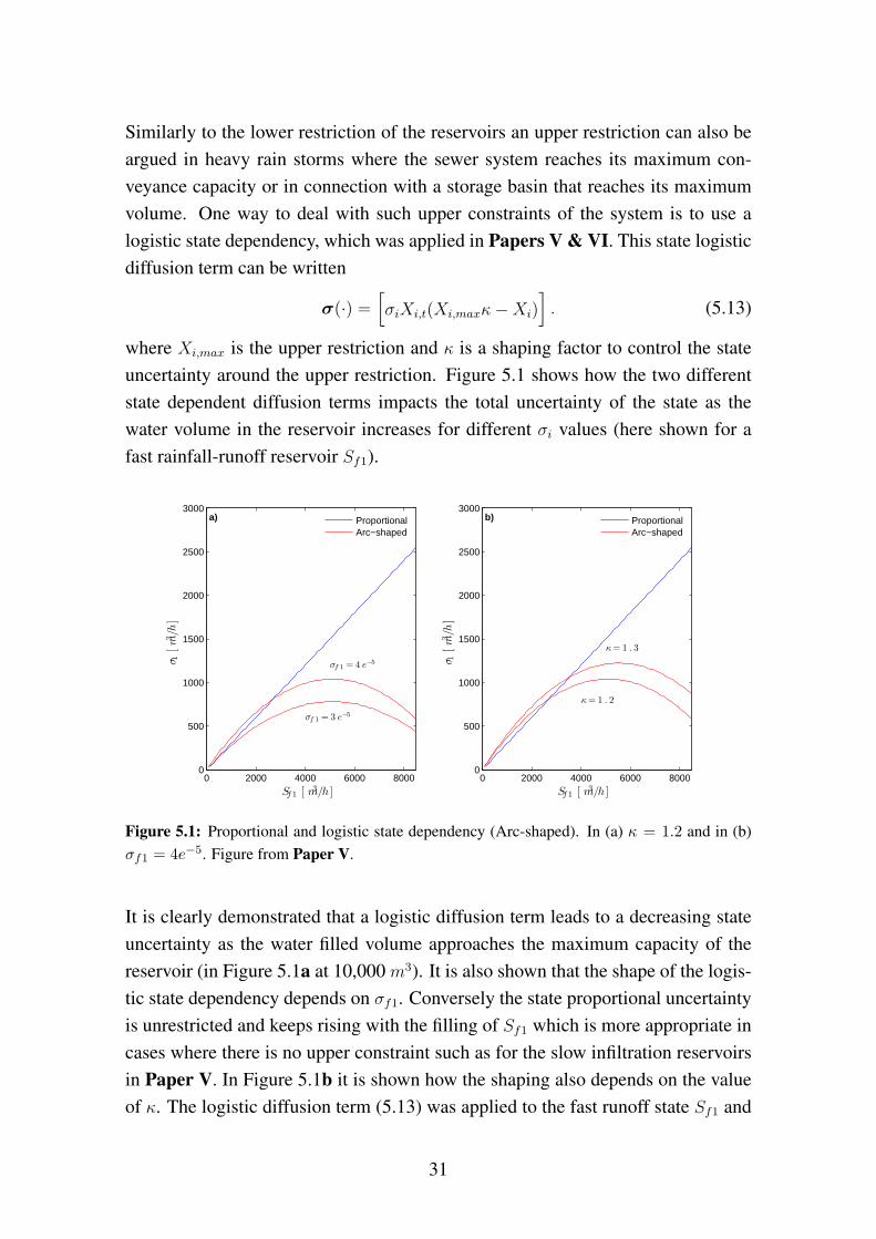
Similarly to the lower restriction of the reservoirs an upper restriction can also beargued in heavy rain storms where the sewer system reaches its maximum con-veyance capacity or in connection with a storage basin that reaches its maximumvolume. One way to deal with such upper constraints of the system is to use alogistic state dependency, which was applied in Papers V & VI. This state logisticdiffusion term can be written
σ(·) =[σiXi,t(Xi,maxκ−Xi)
]. (5.13)
where Xi,max is the upper restriction and κ is a shaping factor to control the stateuncertainty around the upper restriction. Figure 5.1 shows how the two differentstate dependent diffusion terms impacts the total uncertainty of the state as thewater volume in the reservoir increases for different σi values (here shown for afast rainfall-runoff reservoir Sf1).
0 2000 4000 6000 80000
500
1000
1500
2000
2500
3000
σ 1[m3
/h]
σf 1 = 3 e−5
σf 1 = 4 e−5
a)
Sf1 [ m3/h ]
ProportionalArc−shaped
0 2000 4000 6000 80000
500
1000
1500
2000
2500
3000
κ = 1 . 2
κ = 1 . 3
b)
σ 1[m3
/h]
Sf1 [ m3/h ]
ProportionalArc−shaped
Figure 5.1: Proportional and logistic state dependency (Arc-shaped). In (a) κ = 1.2 and in (b)σf1 = 4e−5. Figure from Paper V.
It is clearly demonstrated that a logistic diffusion term leads to a decreasing stateuncertainty as the water filled volume approaches the maximum capacity of thereservoir (in Figure 5.1a at 10,000 m3). It is also shown that the shape of the logis-tic state dependency depends on σf1. Conversely the state proportional uncertaintyis unrestricted and keeps rising with the filling of Sf1 which is more appropriate incases where there is no upper constraint such as for the slow infiltration reservoirsin Paper V. In Figure 5.1b it is shown how the shaping also depends on the valueof κ. The logistic diffusion term (5.13) was applied to the fast runoff state Sf1 and
31
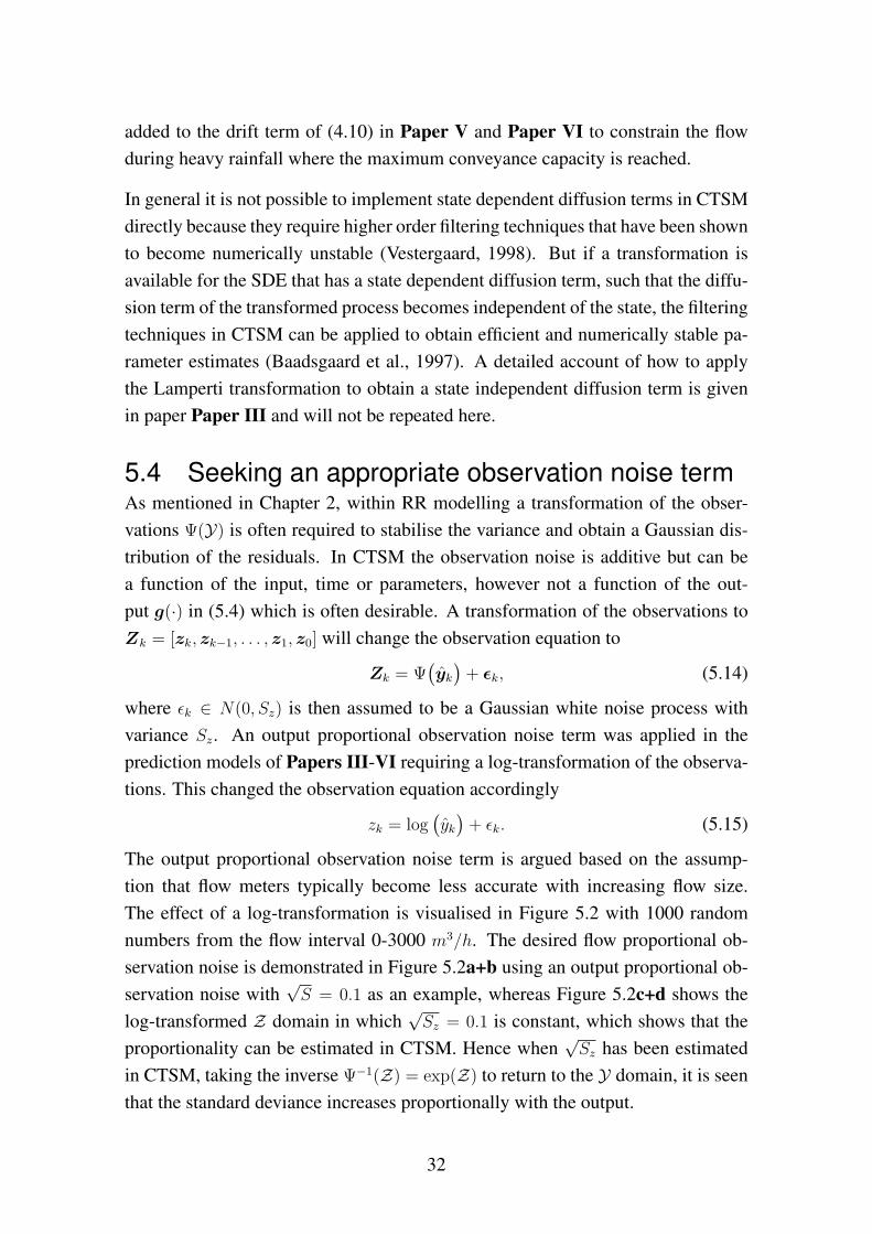
added to the drift term of (4.10) in Paper V and Paper VI to constrain the flowduring heavy rainfall where the maximum conveyance capacity is reached.
In general it is not possible to implement state dependent diffusion terms in CTSMdirectly because they require higher order filtering techniques that have been shownto become numerically unstable (Vestergaard, 1998). But if a transformation isavailable for the SDE that has a state dependent diffusion term, such that the diffu-sion term of the transformed process becomes independent of the state, the filteringtechniques in CTSM can be applied to obtain efficient and numerically stable pa-rameter estimates (Baadsgaard et al., 1997). A detailed account of how to applythe Lamperti transformation to obtain a state independent diffusion term is givenin paper Paper III and will not be repeated here.
5.4 Seeking an appropriate observation noise termAs mentioned in Chapter 2, within RR modelling a transformation of the obser-vations Ψ(Y) is often required to stabilise the variance and obtain a Gaussian dis-tribution of the residuals. In CTSM the observation noise is additive but can bea function of the input, time or parameters, however not a function of the out-put g(·) in (5.4) which is often desirable. A transformation of the observations toZk = [zk, zk−1, . . . , z1, z0] will change the observation equation to
Zk = Ψ(yk
)+ ϵk, (5.14)
where ϵk ∈ N(0, Sz) is then assumed to be a Gaussian white noise process withvariance Sz. An output proportional observation noise term was applied in theprediction models of Papers III-VI requiring a log-transformation of the observa-tions. This changed the observation equation accordingly
zk = log(yk)+ ϵk. (5.15)
The output proportional observation noise term is argued based on the assump-tion that flow meters typically become less accurate with increasing flow size.The effect of a log-transformation is visualised in Figure 5.2 with 1000 randomnumbers from the flow interval 0-3000 m3/h. The desired flow proportional ob-servation noise is demonstrated in Figure 5.2a+b using an output proportional ob-servation noise with
√S = 0.1 as an example, whereas Figure 5.2c+d shows the
log-transformed Z domain in which√Sz = 0.1 is constant, which shows that the
proportionality can be estimated in CTSM. Hence when√Sz has been estimated
in CTSM, taking the inverse Ψ−1(Z) = exp(Z) to return to the Y domain, it is seenthat the standard deviance increases proportionally with the output.
32
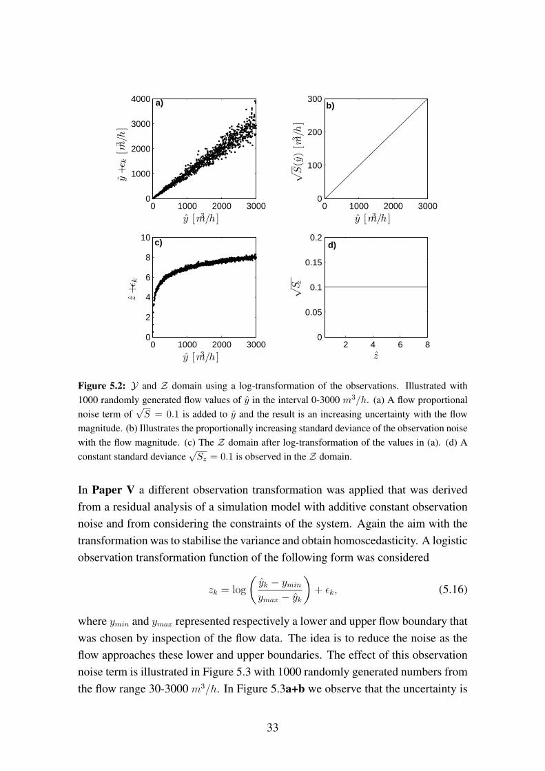
0 1000 2000 30000
2
4
6
8
10
y [m3/h ]
z+ε k
c)
2 4 6 80
0.05
0.1
0.15
0.2
z
√
S z
d)
0 1000 2000 30000
1000
2000
3000
4000
y [m3/h ]
y+e k
[m3/h
]
a)
0 1000 2000 30000
100
200
300
y [m3/h ]
√
S(y
)[m
3/h
]
b)
Figure 5.2: Y and Z domain using a log-transformation of the observations. Illustrated with1000 randomly generated flow values of y in the interval 0-3000 m3/h. (a) A flow proportionalnoise term of
√S = 0.1 is added to y and the result is an increasing uncertainty with the flow
magnitude. (b) Illustrates the proportionally increasing standard deviance of the observation noisewith the flow magnitude. (c) The Z domain after log-transformation of the values in (a). (d) Aconstant standard deviance
√Sz = 0.1 is observed in the Z domain.
In Paper V a different observation transformation was applied that was derivedfrom a residual analysis of a simulation model with additive constant observationnoise and from considering the constraints of the system. Again the aim with thetransformation was to stabilise the variance and obtain homoscedasticity. A logisticobservation transformation function of the following form was considered
zk = log
(yk − ymin
ymax − yk
)+ ϵk, (5.16)
where ymin and ymax represented respectively a lower and upper flow boundary thatwas chosen by inspection of the flow data. The idea is to reduce the noise as theflow approaches these lower and upper boundaries. The effect of this observationnoise term is illustrated in Figure 5.3 with 1000 randomly generated numbers fromthe flow range 30-3000 m3/h. In Figure 5.3a+b we observe that the uncertainty is
33
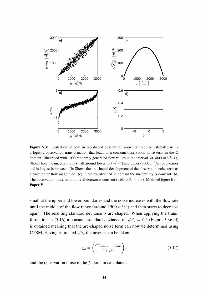
0 1000 2000 3000
−5
0
5
y [m3/h ]
z+ε k
c)
−5 0 50
0.2
0.4
0.6
z
√
S z
d)
0 1000 2000 30000
1000
2000
3000
y [m3/h ]
y+e k
[m3/h
]
a)
0 1000 2000 30000
100
200
300
y [m3/h ]
√
S(y
)[m
3/h
]
d)
Figure 5.3: Illustration of how an arc-shaped observation noise term can be estimated usinga logistic observation transformation that leads to a constant observation noise term in the Zdomain. Illustrated with 1000 randomly generated flow values in the interval 30-3000 m3/h. (a)Shows how the uncertainty is small around lower (30 m3/h) and upper (3000 m3/h) boundariesand is largest in between. (b) Shows the arc-shaped development of the observation noise term asa function of flow magnitude. (c) In the transformed Z domain the uncertainty is constant. (d)The observation noise term in the Z domain is constant (with
√Sz = 0.3). Modified figure from
Paper V.
small at the upper and lower boundaries and the noise increases with the flow rateuntil the middle of the flow range (around 1500 m3/h) and then starts to decreaseagain. The resulting standard deviance is arc-shaped. When applying the trans-formation in (5.16) a constant standard deviance of
√Sz = 0.3 (Figure 5.3c+d)
is obtained meaning that the arc-shaped noise term can now be determined usingCTSM. Having estimated
√Sz the inverse can be taken
yk =
(ezkymax + ymin
1 + ezk
), (5.17)
and the observation noise in the Y domain calculated.
34
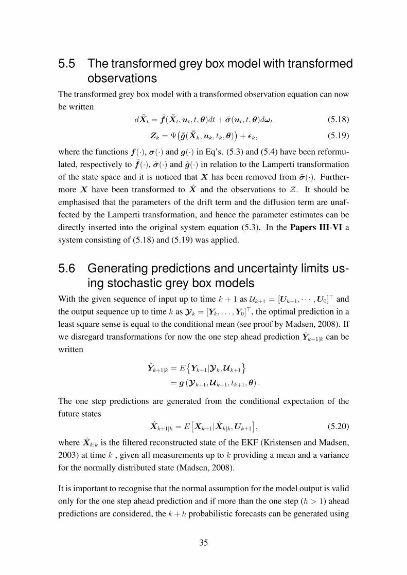
5.5 The transformed grey box model with transformedobservations
The transformed grey box model with a transformed observation equation can nowbe written
dXt = f(Xt,ut, t,θ)dt+ σ(ut, t,θ)dωt (5.18)
Zk = Ψ(g(Xk,uk, tk,θ)
)+ ϵk, (5.19)
where the functions f(·), σ(·) and g(·) in Eq’s. (5.3) and (5.4) have been reformu-lated, respectively to f(·), σ(·) and g(·) in relation to the Lamperti transformationof the state space and it is noticed that X has been removed from σ(·). Further-more X have been transformed to X and the observations to Z. It should beemphasised that the parameters of the drift term and the diffusion term are unaf-fected by the Lamperti transformation, and hence the parameter estimates can bedirectly inserted into the original system equation (5.3). In the Papers III-VI asystem consisting of (5.18) and (5.19) was applied.
5.6 Generating predictions and uncertainty limits us-ing stochastic grey box models
With the given sequence of input up to time k + 1 as Uk+1 = [Uk+1, · · · ,U0]⊤ and
the output sequence up to time k as Yk = [Yk, . . . ,Y0]⊤, the optimal prediction in a
least square sense is equal to the conditional mean (see proof by Madsen, 2008). Ifwe disregard transformations for now the one step ahead prediction Yk+1|k can bewritten
Yk+1|k = E{Yk+1|Yk,Uk+1
}= g (Yk+1,Uk+1, tk+1,θ) .
The one step predictions are generated from the conditional expectation of thefuture states
Xk+1|k = E[Xk+1|Xk|k,Uk+1
], (5.20)
where Xk|k is the filtered reconstructed state of the EKF (Kristensen and Madsen,2003) at time k , given all measurements up to k providing a mean and a variancefor the normally distributed state (Madsen, 2008).
It is important to recognise that the normal assumption for the model output is validonly for the one step ahead prediction and if more than the one step (h > 1) aheadpredictions are considered, the k+ h probabilistic forecasts can be generated using
35
a numerical approach (the Euler scheme) for simulating the SDEs of the systemequation (5.3) (Kloeden and Platen, 1999)
Xk+h|k =Xk|k +
( h/∆∑i=1
f(Xk+(i−1)∆|k,Uk+i∆,θ
))∆
+
h/∆∑i=1
σ(Xk+(i−1)∆|k,Uk+i∆,θ
)∆Wk+(i−1)∆.
(5.21)
where ∆ is the time step for the Euler approximation (assumed small), and ∆Wk isa randomly generated increment of the Wiener process {W}k, i.e. ∆Wk = Wk+∆ −Wk. In Papers IV, V & VI the Euler scheme was applied with ∆ = 1 minute
which means that 15 euler steps were taken per prediction step in the models.
With an increasing prediction horizon (h > 1) the variance of the stochastic termXk+h|k increases and the accuracy of a single point prediction, generated from(5.21), is reduced. To obtain a predictive distribution of the h step ahead predictiona high number of state simulations are needed for each ∆ step and 1000 was con-sidered an adequate number in the papers mentioned above. Thus at all the ∆’s therequired 1000 simulations are run with (5.21). At the desired prediction step k + h
the 1000 predicted states are inserted in the observation equation (5.19) to obtain1000 predicted output values Zk+h|k.
A predictive empirical distribution can be profiled by sorting the 1000 predictedoutputs from the highest (rank 1) to the lowest (rank 1000) value. For example toobtain the 90% bounds the lower bound is found at rank 950 and the upper at rank50 and the median is found at rank 500. Following this example all the desiredquantiles can be estimated.
For a simulation model without diffusion terms the uncertainty bounds are simplyderived from the assumed normally distributed observation noise term (5.4).
36
6 The epistemic approach to uncertaintyevaluationThe generalised likelihood estimation (GLUE) methodology is considered an epis-temic method to uncertainty evaluation (Beven et al., 2011) and is described in thisChapter.
6.1 Introducing stochastic parametersIn the GLUE methodology the deterministic model formulation is once again con-sidered
dXt = f(Xt,Ut, t,θstoch.var.
)dt (6.1)
Yk = g(Xk,Uk, tk,θstoch.var.
), (6.2)
and stochasticity is introduced by interpreting the parameters as stochastic vari-ables. By doing so the need for stochastic model terms such as the diffusion andobservation noise terms in the grey box model is unnecessary and model errorsare instead implicitly accounted for by uncertainty in the parameters. This is incontrast to the interpretation of the stochastic approach outlined in Chapter 5 inwhich the parameters have constant but uncertain values. GLUE acknowledges theexistence of many (almost) equally well performing parameter sets, a phenomenonreferred to as equifinality by GLUE users (Beven, 2006).
6.2 The pseudo-Bayesian approachIn GLUE, a prior likelihood of each parameter set Θi is specified L0 (Θi), typicallya non-informative uniform prior is chosen, and a likelihood measure L (Θi|Y) isselected such that a posterior likelihood Lp (Θi|Y) can be found from Bayes equa-tion
Lp (Θi|Y) =L0 (Θi)L (Θi|Y)
C, (6.3)
where C is a scaling constant to ensure that the cumulative of all the parameter setsis unity (Beven and Binley, 1992; Beven and Freer, 2001; Beven, 2012).
Most often an informal likelihood measure is applied, and many different variantshave been suggested (Freer et al., 1996; Beven and Freer, 2001; Thorndahl et al.,2008; Freni et al., 2009a). Having chosen a likelihood measure for parameter setevaluation a choice regarding which parameters to retain for predictive analysis
37
needs to be taken before the posterior parameter distribution can be summarised.Because of these subjective choices the term pseudo-Bayesian was used by Man-tovan and Todini (2006); Freni et al. (2009b).
6.3 Choosing a likelihood measure and the behav-ioral parameter sets
In Paper II two different likelihood measures was chosen; one for dry weather pe-riods Ldw and one for wet weather periods Lww, and the periods were differentiatedby a flow threshold of 0.15 m3/s
Ldw = 1− σ2ϵ
σ2o
, σ2o > σ2
ϵ & Y1 ∈(Y < 0.15m3/s
)(6.4)
Lww = e−H
(σ2ϵ
σ2o
), Y2 ∈
(Y ≥ 0.15m3/s
), (6.5)
where σ2ϵ is the residual error variance, σ2
o is the observation variance, Y1 denotesthe dry weather observations, Y2 denotes the wet weather observations and H isa shaping factor that was fixed to 1. A combined likelihood measure inspired byChoi and Beven (2007) was then calculated by multiplication of the dry and wetweather likelihoods
L (θ|Y) = ϖ1Ldwϖ2Lww, (6.6)
where ϖ1 and ϖ2 are weighting coefficients both set to 1, hence the model per-formance in dry and wet weather periods is equally weighted even though the dryweather period amounts 80% of the whole period considered. The more positivethe likelihood values are, the better. Parameter sets returning negative likelihoodvalues are not included because in that case the observed mean would be a betterpredictor than the model.
In a comparative study for describing the flow simulation uncertainty in Section8.3, the GLUE method is compared with the grey box approach. In this studythe Nash-Sutcliffe model efficiency coefficient (NS) is used as likelihood measurewhich is defined in (6.4), however in this case without subdividing flow data intodry and wet weather periods. This was chosen because the scope was to compare atraditional GLUE uncertainty analysis normally based on NSE with the stochasticapproach.
The choice of which parameter sets to accept and which to reject is completely sub-jective but commonly GLUE users resort to a "statistical" approach in this choice
38
and demands that the GLUE generated simulation limits encompass a consistentproportion of the observations (Lindblom et al., 2011; Vezzaro and Mikkelsen,2012). This approach was adopted in both GLUE studies (Paper II and the com-parative study to be reported in Section 8.3). In Paper II we aimed at covering90% of the observations by the 90% uncertainty bounds and in the comparativestudy this was extended to include ten "quantiles" , see Chapter 7.
6.4 Searching the parameter spaceBefore the parameter space can be searched an appropriate distribution and pa-rameter range for each parameter needs to be specified. In Paper II a uniformdistribution was used for all parameters but a reasonable prior range for each pa-rameter was not easily decided and a broad range was therefore initially selected.In general two methods for searching the parameter space are applied, either a plainMonte Carlo method and its more efficient counterpart Latin Hypercube Sampling(LHS) that both search randomly (Thorndahl et al., 2008; Freni et al., 2009b; Jinet al., 2010; Li et al., 2010), or a Markov Chain Monte Carlo method (MCMC)(Blasone et al., 2008; McMillan and Clark, 2009; Lindblom et al., 2011; Vezzaroand Mikkelsen, 2012) that is designed to locate the high performing areas of theparameter space in an efficient and intelligent way.
The LHS technique was used in Paper II, and initially 100,000 random parametersets were generated and so-called dotty plots (Beven, 2009a) were then studiedto locate the higher likelihood areas. The parameter ranges were then adjustedaccordingly and a new LHS started. Finally likelihood values of 200,000 parametersets were produced of which 18,720 returned positive values and therefore wereretained for further analysis.
In the comparative study it was decided to take advantage of an MCMC samplingmethod as other GLUE users have advocated for, the advantage being less com-putation time and avoidance of iterative prior range specification. Two MCMCschemes were investigated, initially the DRAM schme developed by Haario et al.(2006) and secondly the DREAM (DiffeRential Evolution Adaptive Metropolis)scheme developed by Vrugt et al. (2009c), however DREAM was found to be muchmore effective in finding the high performance parameter sets and this scheme wastherefore chosen. The algorithm will not be detailed here and the reader is referredto Vrugt et al. (2009a,c) and Vrugt (2011) for more information. With its defaultsettings and a formal likelihood function the DREAM scheme proved to be ex-
39
tremely effective in locating the best performing parameter sets and adjustmentswere therefore necessary to ensure more frequent visits of lower likelihood areas.McMillan and Clark (2009) describe a way to implement the NS likelihood mea-sure in the SCEM-UA algorithm which is the predecessor of DREAM. They arguethat in order for NS to be used in the algorithm it must be nonnegative and mono-tonically increasing with improved performance. To meet the former condition, theNS is set to zero when negative values are returned. The NS is only used via theposterior density ratio R of two samples, which can be expressed in the followingform
R =1− σ2
ϵ1
σ2o
1− σ2ϵ2
σ2o
=σ2o − σ2
ϵ1
σ2o − σ2
ϵ2
=K − SSE1
K − SSE2
, (6.7)
where K is a constant. However they found that the chain only slowly migratedtowards high-performance regions due to two issues: (1) Poor representation ofrelative model performance and (2) Lack of ability to order poor model fits. Forexample the probability of moving from 0.9 to 0.8 is quite high as the posteriordensity ratio is 0.8/0.9 = 0.89. To deal with this issue K can be reduced whichcauses higher weight to be placed on small improvements in NSE. To addressissue 2, the exact sums of squared error scores (SSE) were retained such that allmodel fits could be correctly ordered, even though this information was not used tocalculate the ratio R. Lindblom et al. (2011) suggested a slightly different posteriordensity ratio
R =exp(−SSE1/T )
exp(−SSE2/T ), (6.8)
where T is a scaling factor that is manually adjusted until a certain proportion of theobservations are covered by the simulation limits. None of the suggestions resultedin a completely satisfactory exploration of the parameter space but inspired to thefollowing posterior density ratio
R =
(1− SSE1/T
1− SSE2/T
)−J
, (6.9)
where T was chosen lower than σ2o and J is an even number manually adjusted
until a satisfactory distribution of low and high likelihood values are found. Theoriginal SSE values were retained as recommended.
6.5 Generating uncertainty limitsTo obtain the uncertainty limits the posterior likelihood values of all the K be-havioural parameter sets ΘB,i were calculated using (6.3). To each time step k the
40
ith simulated flow Y ksim,i produced by the behavioural parameter set ΘB,i and its
associated posterior likelihood Lp (ΘB,i) value is sorted in descending order withrespect to flow magnitude. For example the 95% upper simulation limit can befound by summation of posterior likelihood values from the highest flow value anddownwards until
K∑i=1
Lp (ΘB,i) = 0.05,
and likewise the lower 95% simulation limit can be obtained by
K∑i=1
Lp (ΘB,i) = 0.95.
The lower and upper bounds form the 95% simulation limits. Similarly other sim-ulation limits can be derived.
41

42
7 Benchmarking models and uncertaintyapproaches7.1 Residual analysisFor the stochastic approach the statistical assumptions underlying the model shouldbe tested by analysing the model residuals for structure, dependence, normality andhomoscedasticity. The following tests are all described in Madsen (2008).
• The structure of the residuals should be inspected by plotting the standardisedresiduals (std.residuals) as a function of the observations. If the statisticalassumptions are met the std.residuals appear randomly scattered about zero,there should not be many std.residuals with magnitudes greater than 3, andmost of the std.residuals should have values less than 2.
• The std.residuals should also be checked for dependence and ideally they areindependent of each other. The autocorrelation function (ACF) and the partialautocorrelation function (PACF) can be used to check that the std.residualsare not serially autocorrelated.
• The std.residuals should also be normally distributed, and this can be exam-ined by a quantile-quantile (QQ) plot or by the cumulative periodogram. Inboth tests a straight line indicates a normal distribution.
• Finally the std.residuals should be tested for variance homogeneity (homoscedas-ticity) which means that the variance of the std.residuals is constant acrossobservations. If the variance changes with the flow magnitude (heteroscedas-ticity) some transformation of the observations (log-transform, square root, orsome Box-Cox transformation) may be required to stabilise the variance.
Residual analyses was performed in Papers III and V.
7.2 Probabilistic prediction and simulation measuresThe scope with model development is to use the models for making predictionsand/or for simulation and assess the associated uncertainty (Gneiting et al., 2007;Gneiting and Raftery, 2007). Therefore it is meaningful to evaluate the proba-bilistic prediction and simulation performance, and hence not only consider theresiduals. To do so we should first consider the reliability of the predictions or thesimulation.
43
7.2.1 Reliability biasA prediction or simulation interval I(β) of a given quantile level β is defined as
I(β) = [Y (l); Y (u)] (7.1)
where Y (l) and Y (u) are respectively the lower and upper limits of the model outputat levels β/2 and 1 − β/2. The interval is reliable if the observed coverage n(β)
matches the nominal coverage 1 − β β ∈ [0; 1]. For example if we consider the90% prediction interval I(0.1) we should expect to cover 90% of the observations.The reliability bias can be defined as the discrepancy between the nominal andobserved coverage
b(β) = 1− β − n(β) (7.2)
and hence the ideal reliability bias is b(β) = 0. It is seen from (7.2) that if the predic-tion interval covers more observations than expected then b(β) < 0, and a negativebias is observed, and conversely if the prediction interval covers less observationsthan expected, i.e. b(β) > 0, this would entail a positive bias. The reliability biaswas calculated in Papers IV-VI wheras in Paper II the term coverage ratio (CR)was applied which is simply the fraction of observations covered by the predictionlimits.
7.2.2 SharpnessThe sharpness (Gneiting et al., 2007) is a measure of the average size of the pre-diction/simulation interval which is relevant because in general we are interestedin obtaining as narrow bounds as possible, while still reliable. Thus the sharper theintervals the more narrow. Sharpness is defined as
δ(β)
=1
K
K∑k=1
(y(u)k − y
(l)k
), (7.3)
where y(u)k and y
(l)k represent, respectively, the upper and lower limits of the output
at any given time step k and quantile level β of the entire period K. The termsharpness were used in Papers IV-Paper VI and in Paper II another designationthe average band width (ABW) was used synonymously and the related term av-erage relative interval length (ARIL) that measures the relative uncertainty of thebounds
ARIL =1
N
N∑t=1
(y(u)k − y
(l)k
yk
), (7.4)
where yk is the observed output. Hence ARIL can be used to compare uncertaintiesobtained from different study areas or study periods (Jin et al., 2010).
44
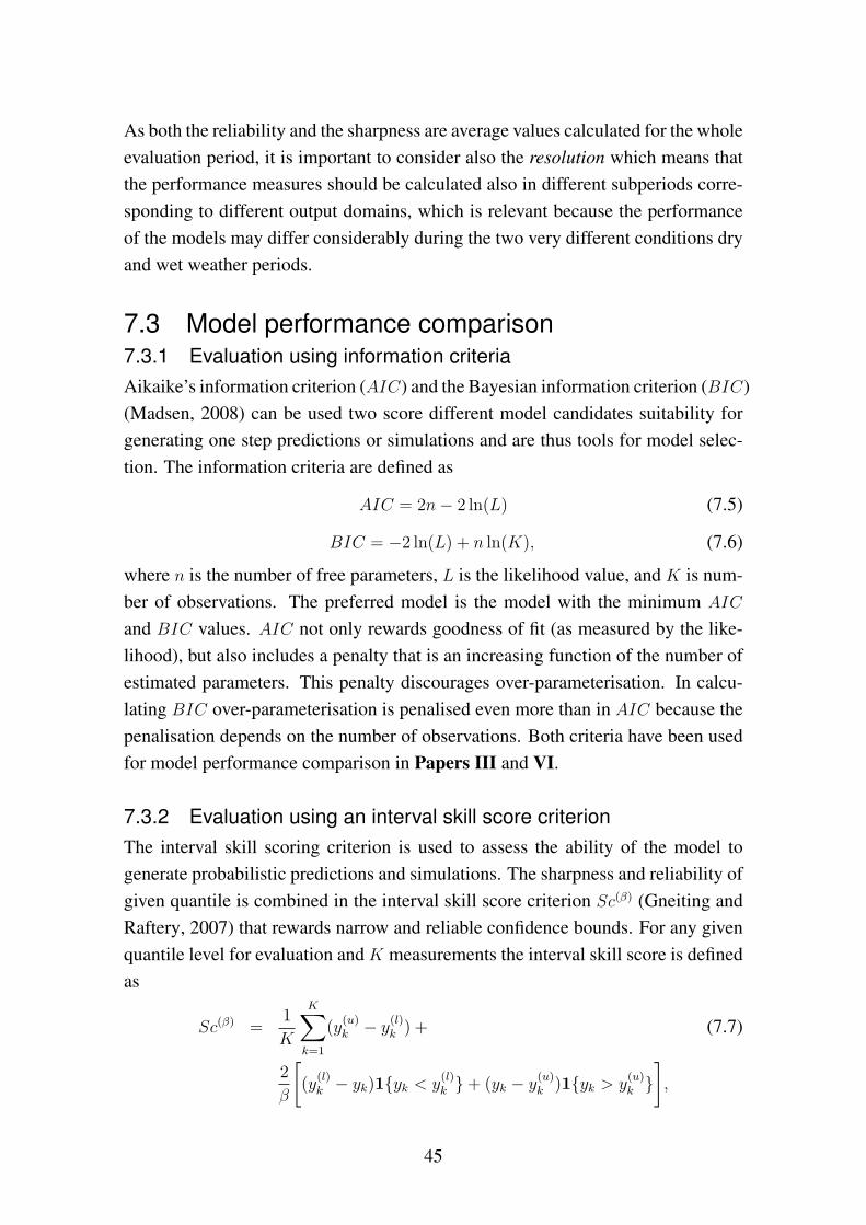
As both the reliability and the sharpness are average values calculated for the wholeevaluation period, it is important to consider also the resolution which means thatthe performance measures should be calculated also in different subperiods corre-sponding to different output domains, which is relevant because the performanceof the models may differ considerably during the two very different conditions dryand wet weather periods.
7.3 Model performance comparison7.3.1 Evaluation using information criteriaAikaike’s information criterion (AIC) and the Bayesian information criterion (BIC)(Madsen, 2008) can be used two score different model candidates suitability forgenerating one step predictions or simulations and are thus tools for model selec-tion. The information criteria are defined as
AIC = 2n− 2 ln(L) (7.5)
BIC = −2 ln(L) + n ln(K), (7.6)
where n is the number of free parameters, L is the likelihood value, and K is num-ber of observations. The preferred model is the model with the minimum AIC
and BIC values. AIC not only rewards goodness of fit (as measured by the like-lihood), but also includes a penalty that is an increasing function of the number ofestimated parameters. This penalty discourages over-parameterisation. In calcu-lating BIC over-parameterisation is penalised even more than in AIC because thepenalisation depends on the number of observations. Both criteria have been usedfor model performance comparison in Papers III and VI.
7.3.2 Evaluation using an interval skill score criterionThe interval skill scoring criterion is used to assess the ability of the model togenerate probabilistic predictions and simulations. The sharpness and reliability ofgiven quantile is combined in the interval skill score criterion Sc(β) (Gneiting andRaftery, 2007) that rewards narrow and reliable confidence bounds. For any givenquantile level for evaluation and K measurements the interval skill score is definedas
Sc(β) =1
K
K∑k=1
(y(u)k − y
(l)k ) + (7.7)
2
β
[(y
(l)k − yk)1{yk < y
(l)k }+ (yk − y
(u)k )1{yk > y
(u)k }],
45

where the indicator 1 is one if the condition is true. In case the observation missesthe quantile interval a penalty is incurred which depends on the considered quan-tile level, meaning that an observation miss at the 95% confidence interval is muchmore expensive than a miss at e.g. the 5% confidence interval. Thus, the smallerthe interval skill score the better the probabilistic prediction performance of themodel, and so Sc(β) can be used to evaluate the different models’ probabilistic per-formance and eventually to select a preferred model. It is noted that the skill scoreis suitable for comparison at different prediction horizons, which the AIC andBIC criteria are not. The skill score was used for model comparison in Papers IV,V and VI and also used to compare the simulation performance of the stochasticapproach and the GLUE approach in Section 8.3.
46
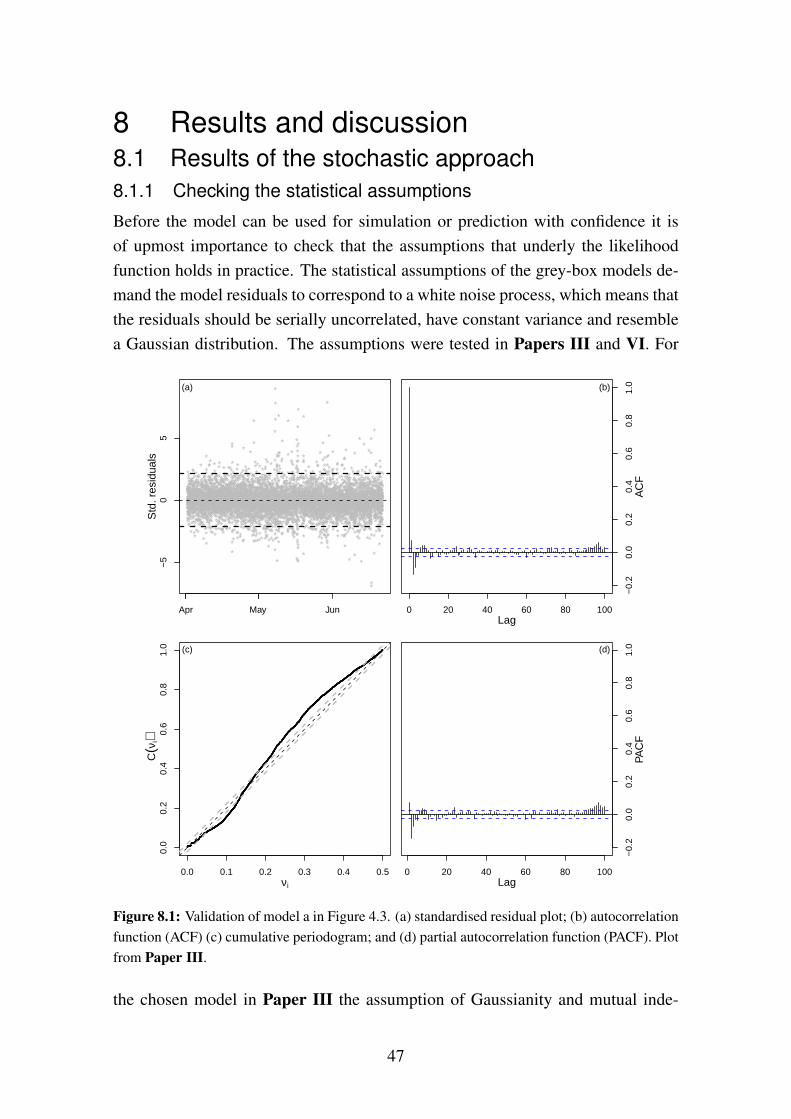
8 Results and discussion8.1 Results of the stochastic approach8.1.1 Checking the statistical assumptions
Before the model can be used for simulation or prediction with confidence it isof upmost importance to check that the assumptions that underly the likelihoodfunction holds in practice. The statistical assumptions of the grey-box models de-mand the model residuals to correspond to a white noise process, which means thatthe residuals should be serially uncorrelated, have constant variance and resemblea Gaussian distribution. The assumptions were tested in Papers III and VI. For
**
**
**
*****
***
*
***
*
*
*
*****
*
****
*******
*
***
****
*
****
******
*
*
***
**
*
**
*
***
**
**
*
****
**
*
**********
**
***
**
**
*
**
***
**
**
*
*********
*
**
***
*****
****
*
****
**
****
*
*
****
**********
*
****
******
*
***
*
*********
*
**
*
**
**
***
*******
***********
*
*
****
*****
*
*
*
*******
*
****
*
*
****
**
**
*
***************
*
****
*
*
****
*
**
*
*******
*
*
******
*
**
*
******
***
*
*******
**
*************
*
***************
*
*
************
*
**
***
**
*******
*
*
*
***********
***
**
*
****
*
*
*
***
**
*
*************
*
*
*
***
*
**
***
***
**
*
*
*
*
*
*****
*
*****
**
********
*****
*
*****
*
****
*
*******
*
******
**
****
**
******
*
*
**
****
*******
*
*
*
***
*
*
***
**
*
*
*
*******
*
*
*
*
****
**
*****
**
****
*
*
*
*
*****
*
*
*
**
**
********
*
***********
*
*
*
*
*
*
*
*********
*
*
*
**
*
*******
*
*
********
*
*****
*
*
****
**
*
**
*
******
*
**
*
*
*
*****
*
*******
*
*
*****
*
*
**
***
*
*
*
*****
********
*
***
*
*****
****
**
**
***
**********
*
*****
**
*
*
*
*
**
***
*******
****
**
*
*
*
*
*
*****
*
****
*
*****
****
*
**********
****
*
**
***
***
******
*
***
*
**
***************
**
***
*********
**
**
*
*
**
*
***
**
***
********
*
*
********
*
**
*
*
*
***
*
**
*
*
*
*
********
*
**********
****
*
**********
*
*
**
***
*
*
******
*
*
*
*
**
*
**
*
*****
*
********
*
**
*******
*
********
*
****
**
***
*
**
******
*****************************
*********
*******
*
*
***
*********
**
****
*
*
**
**
*
**
*********
*
****
*
*********
*******
**
*
*
*
*
*
****
**
*
*
*
*
*
*
*******
**
*
****
****
***
**
***********
*
**
*
*
*
********
**
*************
**
***
**********
**
*
**
*******
*
******
*
*******
*
*
*
*
**********
*
*
*
**
*
***************
**
*
******
**
**
*
*
****
*
*
******
*
***
*
**
*****
*
*
*
*
**
*
*
*
*****
***
*
**
***
**
****
**
******
*
*****
**
*
********
*
*
*
****
*
****
*
*
*
******
**
**
*
**
*******
*
****
**********
*
****
**
*****
*
****
*
*
******
*
****
*********
*
**
*
***
**
**
*
*
**
*
***
**
*
************
*
*
*
***
*
**********
***
***
*
****
***
*
*
*********
**
**
**
*
*******
*
*****
*
***
*
*********
*
***
*
****
*
*
*
*****
********
**
***
*
*******
****
*
***
**
**********
*
***
*
*
*
*********
********
*
**
*
***
*********
**
***********
*
*
******
*
**
*
*
*********
*****
*******
*
***********
*
***
****
*
*
*
*
***********
*
****
****
*
**
**
***
**
**
*
**
*
**
*
**
*
*************
*******
******
*
***
******
*
*
*
*
**********
*
**
**********
*
**
*****
*
****
******
*
********
*
****
**
**
*****
*
*****
***
******
**
*
*
****
******
*********
*
**
*
**
****
*
**********
*****
**
*
******
*
**
**
*
*
*
*
*
*
*
*
***
*
*
*
**
*
***
*
*
*
*
*
*
*
***
*
***
*****
*
*
*
*
*
****
*
*
*******
*
*
**
*
**
**
*******
***
*****
***
***
****************
*
**
*
****
**
**
*
*
*
***
**
**
*
***
*
*
***
*
*
***
*
**
***
***
**
***
********
*
**
*
*
*
**
*
*
**
*****
*
****
**
****
***
*
*****
********
*
****
*
**
**
*
*
*****
*
*
*
*
*
*
*
*
***
*
*
*
*
*
*
****
*
*
*
*
**
***
****
*
*
*
*
*
***
*
**
*
**
****
**
****
******
**
*****
**
*
*
*************
*
**
******
*
**********
***
**
**
**
**
*
**
*
*
******
***
*
*
*
******
*
*****
**
*******
****
*******
*
**
****
*
*
****
*****************
**
*******
***
****
*
*
*
*
*
*
*
****
**
*
*
*
**
**
*
*****
**
**
***
**
**
****
*
*****
***
*
*****
****
**
*****
*******
*****
**
*
***
*
**
*****
*****
*
*
***********
*
**
*
*
****
**
*
**
**
**
*
***
*
****
**
*
*****
***
*
***
*
****
*******
*
**
***
*
*
*
**
*
*****
*
*
****
*
*
*
*
*
***
**
*
*
*
*
*
**
*
****
*
*******
**
*
****
***
*
*
*
*
*
***
*
*
*
**
*
*
*
*
*
*
*
**
**
********
**
***
*
***
*
*
*
****
***
******
***
*
*
*
**
*
*
*
*
*
****
*******
***
*
**
*
**
**
*
*******
*
*
***
*****
*
********
*
*
**
*
*******
*
*
***
*
*
**
*
**
*
*
*
*
*********
**
******
*
***
*
*****
**
*
******
******
**
****
**
*
**
*
***
*
*
*
****
********
*
***
*
**
**
**
*
**
*
**
*
*
***
*
*
**
*****
*
****
*
***
*
*
**
**
**
***
*****
*
*
**
*
*
*
*
**
*
****
****
***
*
*
**
**
**
**
**
****
****
****
*
*
*
**
*
*****
*
****
*
******
***
**
**
*
**
**
*
*****
****
*
*****
**
*
**
**
*
*
***
*
**********
*
********
********
*
**
**
**
*
*
***
*****
*
*
*
*
*
*
***
*
*
***
***
*
*
*
**
**
*******
*
*
**
*
*
*
*
*
*
*
*
****
*
*
*
*
*
*
*
*****
*
*
**
**
*
**
*
*
*
*
*
*
****
*
*
*
*
***
***
*
*
***
*
*
*
**********
*
*
*
***
*
*
*
***
***
****
****
*
*
**
*
*
*
***********
*
*
*
**
***
********
*
*
*
*
**********
*
*
**
*
***
*
*
*
*****
*
****
****
*
**
*
*
**
*
*
*
*
*
*
*
****
*
******
**
***
*
*
***
****
*
*
*
**
*
***
*
*
*******
*
**
****
*
*
*
*
*
**
*
**
******
*
***
***
*
****
*
*
*************
**
*
*
*
**********
****
***
*
**
***
*
******
*
*
*
**
*
**
*
**
****
*
**********
**
*
*********
**
******
*****************
*
*
*****
*
*
*
**
**
*
*
*
*
***
*
*
**
**
**
*
*
*
***
*
****
*
*
****
***
****
********
***
*
*
*
*
*
******
*
*
*********
*
*
*
*
*
*
*
*
*
*
**
*
*
***
*
**
**
*
*
**
*
*
*
*
*****
*
**
****
*
*
**********
*
******
***
*
*
*
****
*
**
*
*
*
*
*
*
**
*
**
**
****
*
*
*
**
*
*
*
**
*****
*
*********
***
********
*
*
***
*
*******
*********
*
*******
****
*
******
*
*
**
***
*
*
*****
*
*
****
***
*
***
***
*
****
******
*****
*
***
*
*
*
*
***********
***
****
****
*
*
*
*****
**
**
******
*
*
****
**
*
*
*
***
*****
*******
*
***
*
***********
********
**
**
*
****
****
*
***************************
**
**
******
*
**********
**
*
***
*
*
*
*****
*
**
*
***
**
*
*
*****
*********
*
**
*
**
*
***********
***
*****
*
***
*
**
***
*
*
*
****
*
**
**
**
*****
**************************
****
**
*
******************
*
***
*****
*
******
*
*
**
*
*
***
**
*
**
**
*****
***
********
*
*
*****
*
*
****
*
*
*
**********
*
*******
*
*
***
**
*
*
***
*
**
**
***
*
*
**
*
**
********
*
***
*
*
*
*
*
*
*
***
*
**
****
*
*
*
*****
*
****
***
**
*****
*
*
*
*
*
**
*
***
*
*
*
***
**
****
**
**
*
******
*
********
*****
*
*******
*
**
***
******
*****
******
*
*****
**
*
*****
**
*
***
*******
*******
*
**
*
*
*
*
*
*
**
*
*
**
**
*
**
***
*
*
*
*
*
*
*
*
*
*
*
*
*
**
**
*
*
*
*
*
*
*
*
**
*
*
**
*
*
*
*
*
*
**
*
*
*
*
*
*
****
*******
**
*
***********
*******
*
******************
*
***
*****
***
***
**********************
****************
*
*
*
*
***
*****
*****
*****
*
*****
***
*
*******************
**
*********
*
**
*
******
*
*********
***********
**
**
*
*
**
*
*
*
*
*
*
*
*
*
**
***
***
*
****
****
*********
*
*****
*
******
*****
**
*****
*
***
*
****
**
*******
*
*
*
*****
*
**
**
**
*
***
*
*
***
*******
*
*
***
*
***
*
**************
*********
*
*
**
*
**
*************
*
******
*
*
******
***
****
**********
*****
******
*
*
*
*
*
*
*
*
****
***
**
*
***
*******
**********
****
*
*
*
*
****
*
*
*
*
******
*
*
*
**
***
*
*****
**
**
**
*
**
**
**
*
**
**
*
*****
**
*
*
*
***
*
*********
**
*
*
*
***********
***
*
**
****
*
*
*
************
*
*
*
*
*****
*
*****
*****
*
*
****
**
*
***
*
*
**
*
****
**********
************
**
*
**
*
*
*
***
*
*****
******
*****
*********
*
****
****
*
******
*
********
******
*
*
***
**
**
************
*
***
**
***
*
**
*
**
****
*
*
*******
**
******
*
*****
*
********
*
**
*
*
*
***************
*
*
**
*
*
**
**
******
*
***
***
*******
*
**
****
*
***********
*
****
*
***
*
**
******
*
*
****
*
**
*
*
*
*
****
*
**
*********************
****
****
******
*
*
*
*******
*
*
*
**
***
*
**
**
**
*
*
*
*
*******************
**
*
**
*
****
****
**
*
***
*
*
***
*
**
*
*
*******
*
*
***
**
*
*
*
**
*
*
*
***
**
***
*
*
*
**
**********
*
*
**
*
**
*
*****
**
****
*
**
*
*
****
*
*
*
*********
***
*
*****
**
*
**
*
************
***
**
*
*
**********
**
**
*
*
*
*
**
**
*
*
*
*
*
*
**
*
**
*
**
***
*
*
*
*
*
****
***
*****
***
*
*********
***
******
*
*
*
*********************
***
**
****
**
*
*
*********************
**********
**
**
*
*****
*
****
***
***
**
**
*
**
*******************
*
*****
***
***
*******************
*********
*
*
**
*
***
*
*
*
****
**
****
*
*******
*
*
*****
**
*
*
*
*
***
*****
***
****
**
*
**
*****************
*****
****
*
********
*******
**
*
*******
*******
*****
*
**
***
******
******
***
*****
***
***
*
*
*
**
***
**********
*****
*******
***
******
**
*
*****
*
*
*
*
***
***
**
***
****
*
***
*
**********************
**
*****
*****
**
*********
**
***
*************
*
*******
**
******
**
****
****
*
********
***
***
***
**********
*
*
*
***
***
**********
*************
*******
*
*
*
**
**
*
**
*
****
**
****
*
*
*
**
*
*
***
*
*
*
*
***************
****
***
**********
*
*
**********
**************
*********
*
**
**
*
**
******
*
*
**
*
****
**
****
*
*
***
*
***
*
****
***
**
****
***
*
***
*
*****
**
*
*
**
*
**
***
******
*
*
*****
*
****
*
**
*
*
********
**
**
*
****
*
***
**
*
*
**
****
*
**
*****
*
***
*
**
***
*
**
*
*
*
************
*
*
*
*
*****
*
*******
*
*****
*
**
*
*********
*
*
*
*****
****
*
*
********
*
**
*
**
**
*
*
*******
**
**
**
***
*
****
***
***
***********
*******
*
*
******
***
***
*
*****
**
**
*
*******
*
*
**
******
*
**
************
*
*
****
*
**
*
*
**
*
*
***
*
*
*******
**
*
*****
*
*
*
**
**********
******
*
**
*
*
*
*
******
**
**
*
******
*
*
*
*
*
*
*
****
**
***
**
*
*
**
*
****
***
**
*
*
**
******************
**
*
*
*
*******
*
**
*
*
*
**
*******
*
***************
*
*
*
**
**
**
**
*
*
***************
***
*
******
*
**********
******
*
*
**
*
*
*
******
*
***
*
*
****
*
**
*****
*
**
*****
**
**
*
*
*****
*
*
**
*
***
*
**
**
*
*
*
********
***
**
****
************
*
*
*
**
**
*
*****
****
*
*
*
************
**
*
***
**
*****
*
*
**
***
*
*
****
*
*
****
****
***
**
*
****
*
*********
*
**
*
***
**
*
******
****
*
**
***
*
*
***
**
**
*
**
*
****
*
*
**
*
***
**
**********
***
**
*
*
**
*
****
*
*
***************
*
*
******
*
******
*
*
*
*
**
*
****
*******
****
*
**
*
***
**
*******
*
***
*
*****
*****
*
*
*
*
*
***********
*
**
****
*
***********
****
***
*
**
**
**
***
**
*
*
******
*
*
****
*
*
*
***
*******************
**
**
**
*
***
*
***
*
*
**
****
*
*
*
*
********
**
**
*
**
**
*
**
***
*
***
***
*
*
*
*
*
*
*
*
*
***
*
***********
*
**
*
*
*******************************
*
************************
***
**
*
****
****
*
***************************
*
*
*
*
*
*
*
*
*
***************
*
*
*
**
*
*********
***
**************
***
**
**
**
*************
**
*
*
***
*
***
*
**
*******
*
****
*****
*
*
*
*
*********
********
*****
*
********
*****
*
**
*
**
************
*
********
*
**
*
*
****
***
*****
*
***
****
****
*
***
*******
*
**
*
*
*
**
****
*
*
*****
*
**
*
**
*
*
*
*
*
*
*
**
**
*
*
******
*
*
*
*****
*
***
*
*
*******
*****
*
*
*
******
*
*
***
*
**********
*
**
*****
*
*
*
*
*
*
*
*******
*
****
*
**
−5
05
Apr May Jun
(a)
Std
. res
idua
ls
0.0 0.1 0.2 0.3 0.4 0.5
0.0
0.2
0.4
0.6
0.8
1.0 (c)
νi
C(ν
i)
0 20 40 60 80 100
−0.
20.
00.
20.
40.
60.
81.
0(b)
AC
F
Lag
0 20 40 60 80 100
−0.
20.
00.
20.
40.
60.
81.
0(d)PA
CF
Lag
Figure 8.1: Validation of model a in Figure 4.3. (a) standardised residual plot; (b) autocorrelationfunction (ACF) (c) cumulative periodogram; and (d) partial autocorrelation function (PACF). Plotfrom Paper III.
the chosen model in Paper III the assumption of Gaussianity and mutual inde-
47
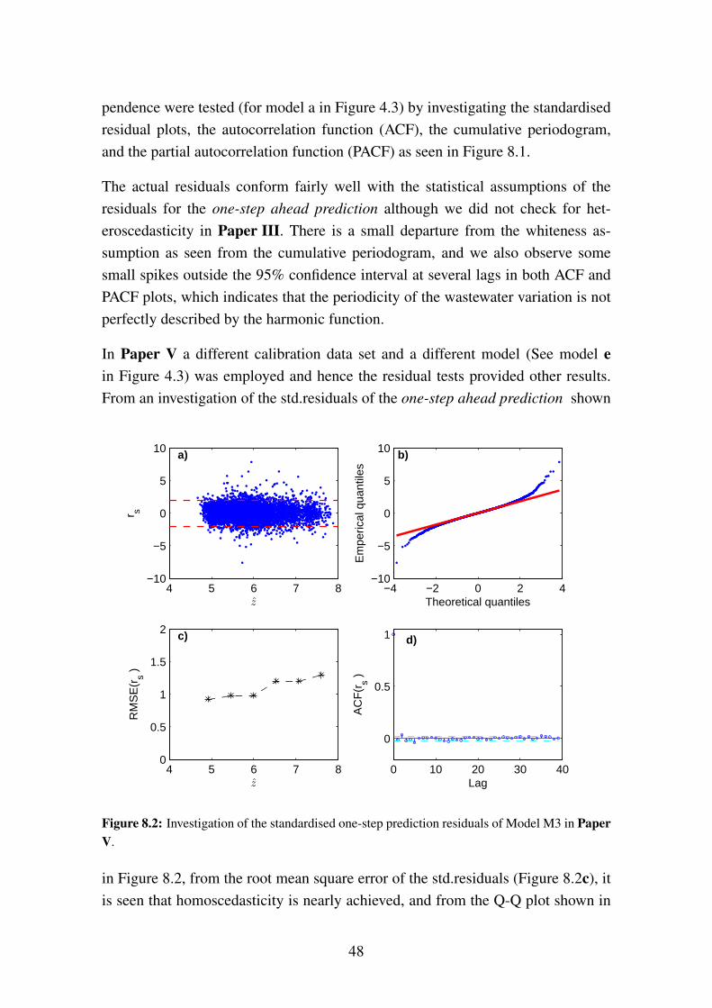
pendence were tested (for model a in Figure 4.3) by investigating the standardisedresidual plots, the autocorrelation function (ACF), the cumulative periodogram,and the partial autocorrelation function (PACF) as seen in Figure 8.1.
The actual residuals conform fairly well with the statistical assumptions of theresiduals for the one-step ahead prediction although we did not check for het-eroscedasticity in Paper III. There is a small departure from the whiteness as-sumption as seen from the cumulative periodogram, and we also observe somesmall spikes outside the 95% confidence interval at several lags in both ACF andPACF plots, which indicates that the periodicity of the wastewater variation is notperfectly described by the harmonic function.
In Paper V a different calibration data set and a different model (See model ein Figure 4.3) was employed and hence the residual tests provided other results.From an investigation of the std.residuals of the one-step ahead prediction shown
4 5 6 7 8−10
−5
0
5
10
r s
z
a)
−4 −2 0 2 4−10
−5
0
5
10
Theoretical quantiles
Em
peric
al q
uant
iles
b)
4 5 6 7 80
0.5
1
1.5
2
RM
SE
(rs )
z
c)
0 10 20 30 40
0
0.5
1
Lag
AC
F(r
s )
d)
Figure 8.2: Investigation of the standardised one-step prediction residuals of Model M3 in PaperV.
in Figure 8.2, from the root mean square error of the std.residuals (Figure 8.2c), itis seen that homoscedasticity is nearly achieved, and from the Q-Q plot shown in
48
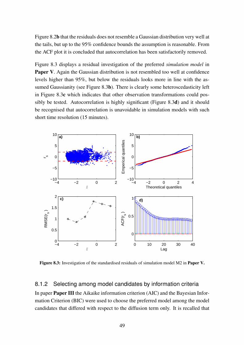
Figure 8.2b that the residuals does not resemble a Gaussian distribution very well atthe tails, but up to the 95% confidence bounds the assumption is reasonable. Fromthe ACF plot it is concluded that autocorrelation has been satisfactorily removed.
Figure 8.3 displays a residual investigation of the preferred simulation model inPaper V. Again the Gaussian distribution is not resembled too well at confidencelevels higher than 95%, but below the residuals looks more in line with the as-sumed Gaussianity (see Figure 8.3b). There is clearly some heteroscedasticity leftin Figure 8.3c which indicates that other observation transformations could pos-sibly be tested. Autocorrelation is highly significant (Figure 8.3d) and it shouldbe recognised that autocorrelation is unavoidable in simulation models with suchshort time resolution (15 minutes).
−4 −2 0 2−10
−5
0
5
10
r s
z
a)
−4 −2 0 2 4−10
−5
0
5
10
Theoretical quantiles
Em
peric
al q
uant
iles
b)
−4 −2 0 20
0.5
1
1.5
2
RM
SE
(rs )
z
c)
0 10 20 30 40
0
0.5
1
Lag
AC
F(r
s )
d)
Figure 8.3: Investigation of the standardised residuals of simulation model M2 in Paper V.
8.1.2 Selecting among model candidates by information criteriaIn paper Paper III the Aikaike information criterion (AIC) and the Bayesian Infor-mation Criterion (BIC) were used to choose the preferred model among the modelcandidates that differed with respect to the diffusion term only. It is recalled that
49
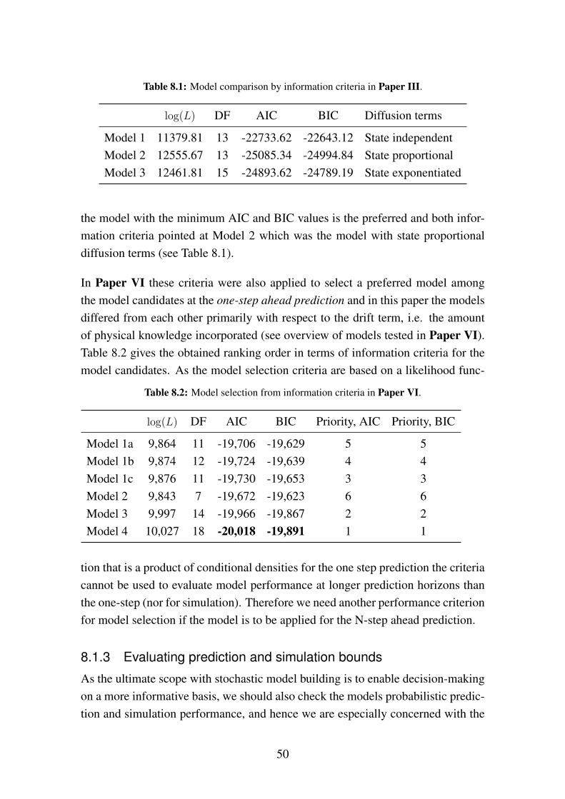
Table 8.1: Model comparison by information criteria in Paper III.
log(L) DF AIC BIC Diffusion terms
Model 1 11379.81 13 -22733.62 -22643.12 State independentModel 2 12555.67 13 -25085.34 -24994.84 State proportionalModel 3 12461.81 15 -24893.62 -24789.19 State exponentiated
the model with the minimum AIC and BIC values is the preferred and both infor-mation criteria pointed at Model 2 which was the model with state proportionaldiffusion terms (see Table 8.1).
In Paper VI these criteria were also applied to select a preferred model amongthe model candidates at the one-step ahead prediction and in this paper the modelsdiffered from each other primarily with respect to the drift term, i.e. the amountof physical knowledge incorporated (see overview of models tested in Paper VI).Table 8.2 gives the obtained ranking order in terms of information criteria for themodel candidates. As the model selection criteria are based on a likelihood func-
Table 8.2: Model selection from information criteria in Paper VI.
log(L) DF AIC BIC Priority, AIC Priority, BIC
Model 1a 9,864 11 -19,706 -19,629 5 5Model 1b 9,874 12 -19,724 -19,639 4 4Model 1c 9,876 11 -19,730 -19,653 3 3Model 2 9,843 7 -19,672 -19,623 6 6Model 3 9,997 14 -19,966 -19,867 2 2Model 4 10,027 18 -20,018 -19,891 1 1
tion that is a product of conditional densities for the one step prediction the criteriacannot be used to evaluate model performance at longer prediction horizons thanthe one-step (nor for simulation). Therefore we need another performance criterionfor model selection if the model is to be applied for the N-step ahead prediction.
8.1.3 Evaluating prediction and simulation bounds
As the ultimate scope with stochastic model building is to enable decision-makingon a more informative basis, we should also check the models probabilistic predic-tion and simulation performance, and hence we are especially concerned with the
50
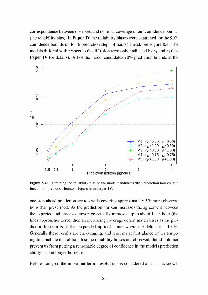
correspondence between observed and nominal coverage of our confidence bounds(the reliability bias). In Paper IV the reliability biases were examined for the 90%confidence bounds up to 16 prediction steps (4 hours) ahead, see Figure 8.4. Themodels differed with respect to the diffusion term only, indicated by γ1 and γ2 (seePaper IV for details). All of the model candidates 90% prediction bounds at the
−0.
050.
000.
050.
10
0.25 0.5 1 2 3 4Prediction horizon [h(hours)]
b h(0.1
)
M1 : (γ1=0.50 , γ2=0.50)M2 : (γ1=1.00 , γ2=0.50)M3 : (γ1=0.50 , γ2=1.00)M4 : (γ1=0.75 , γ2=0.75)M5 : (γ1=1.00 , γ2=1.00)
Figure 8.4: Examining the reliability bias of the model candidates 90% prediction bounds as afunction of prediction horison. Figure from Paper IV.
one step ahead prediction are too wide covering approximately 5% more observa-tions than prescribed. As the prediction horizon increases the agreement betweenthe expected and observed coverage actually improves up to about 1-1.5 hour (thelines approaches zero), then an increasing coverage deficit materialises as the pre-diction horizon is further expanded up to 4 hours where the deficit is 5-10 %.Generally these results are encouraging, and it seems at first glance rather tempt-ing to conclude that although some reliability biases are observed, this should notprevent us from putting a reasonable degree of confidence in the models predictionability also at longer horizons.
Before doing so the important term "resolution" is considered and it is acknowl-
51
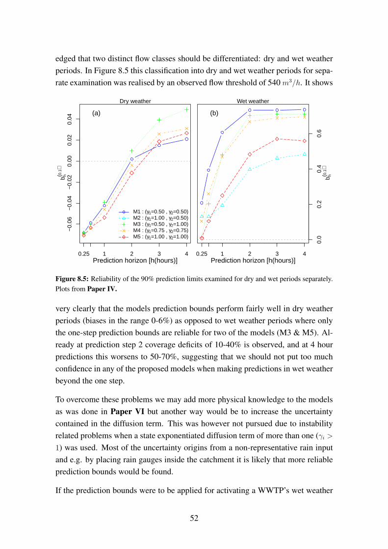
edged that two distinct flow classes should be differentiated: dry and wet weatherperiods. In Figure 8.5 this classification into dry and wet weather periods for sepa-rate examination was realised by an observed flow threshold of 540 m3/h. It shows
−0.
06−
0.04
−0.
020.
000.
020.
04
0.25 1 2 3 4Prediction horizon [h(hours)]
b h(0.1
)
Dry weather
M1 : (γ1=0.50 , γ2=0.50)M2 : (γ1=1.00 , γ2=0.50)M3 : (γ1=0.50 , γ2=1.00)M4 : (γ1=0.75 , γ2=0.75)M5 : (γ1=1.00 , γ2=1.00)
(a)
0.0
0.2
0.4
0.6
0.25 1 2 3 4Prediction horizon [h(hours)]
b h(0.1
)
Wet weather
(b)
Figure 8.5: Reliability of the 90% prediction limits examined for dry and wet periods separately.Plots from Paper IV.
very clearly that the models prediction bounds perform fairly well in dry weatherperiods (biases in the range 0-6%) as opposed to wet weather periods where onlythe one-step prediction bounds are reliable for two of the models (M3 & M5). Al-ready at prediction step 2 coverage deficits of 10-40% is observed, and at 4 hourpredictions this worsens to 50-70%, suggesting that we should not put too muchconfidence in any of the proposed models when making predictions in wet weatherbeyond the one step.
To overcome these problems we may add more physical knowledge to the modelsas was done in Paper VI but another way would be to increase the uncertaintycontained in the diffusion term. This was however not pursued due to instabilityrelated problems when a state exponentiated diffusion term of more than one (γi >1) was used. Most of the uncertainty origins from a non-representative rain inputand e.g. by placing rain gauges inside the catchment it is likely that more reliableprediction bounds would be found.
If the prediction bounds were to be applied for activating a WWTP’s wet weather
52
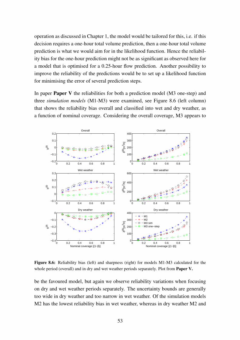
operation as discussed in Chapter 1, the model would be tailored for this, i.e. if thisdecision requires a one-hour total volume prediction, then a one-hour total volumeprediction is what we would aim for in the likelihood function. Hence the reliabil-ity bias for the one-hour prediction might not be as significant as observed here fora model that is optimised for a 0.25-hour flow prediction. Another possibility toimprove the reliability of the predictions would be to set up a likelihood functionfor minimising the error of several prediction steps.
In paper Paper V the reliabilities for both a prediction model (M3 one-step) andthree simulation models (M1-M3) were examined, see Figure 8.6 (left column)that shows the reliability bias overall and classified into wet and dry weather, asa function of nominal coverage. Considering the overall coverage, M3 appears to
0 0.2 0.4 0.6 0.8 1−0.2
−0.1
0
0.1
0.2
b(β)
Overall
0 0.2 0.4 0.6 0.8 1−0.1
0
0.1
0.2
0.3
b(β)
Wet weather
0 0.2 0.4 0.6 0.8 1−0.4
−0.3
−0.2
−0.1
0
Nominal coverage [(1−β)]
b(β)
Dry weather
0 0.2 0.4 0.6 0.8 10
100
200
300
400Overall
δ(β) [m
3 /h]
0 0.2 0.4 0.6 0.8 10
200
400
600Wet weather
δ(β) [m
3 /h]
0 0.2 0.4 0.6 0.8 10
100
200
300
400Dry weather
Nominal coverage [(1−β)]
δ(β) [m
3 /h]
M1M2M3 simM3 one−step
Figure 8.6: Reliability bias (left) and sharpness (right) for models M1-M3 calculated for thewhole period (overall) and in dry and wet weather periods separately. Plot from Paper V.
be the favoured model, but again we observe reliability variations when focusingon dry and wet weather periods separately. The uncertainty bounds are generallytoo wide in dry weather and too narrow in wet weather. Of the simulation modelsM2 has the lowest reliability bias in wet weather, whereas in dry weather M2 and
53
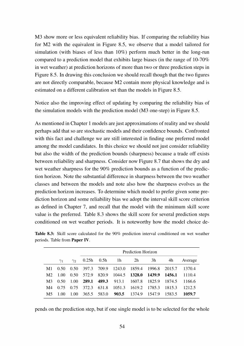
M3 show more or less equivalent reliability bias. If comparing the reliability biasfor M2 with the equivalent in Figure 8.5, we observe that a model tailored forsimulation (with biases of less than 10%) perform much better in the long-runcompared to a prediction model that exhibits large biases (in the range of 10-70%in wet weather) at prediction horizons of more than two or three prediction steps inFigure 8.5. In drawing this conclusion we should recall though that the two figuresare not directly comparable, because M2 contain more physical knowledge and isestimated on a different calibration set than the models in Figure 8.5.
Notice also the improving effect of updating by comparing the reliability bias ofthe simulation models with the prediction model (M3 one-step) in Figure 8.5.
As mentioned in Chapter 1 models are just approximations of reality and we shouldperhaps add that so are stochastic models and their confidence bounds. Confrontedwith this fact and challenge we are still interested in finding one preferred modelamong the model candidates. In this choice we should not just consider reliabilitybut also the width of the prediction bounds (sharpness) because a trade off existsbetween reliability and sharpness. Consider now Figure 8.7 that shows the dry andwet weather sharpness for the 90% prediction bounds as a function of the predic-tion horizon. Note the substantial difference in sharpness between the two weatherclasses and between the models and note also how the sharpness evolves as theprediction horizon increases. To determine which model to prefer given some pre-diction horizon and some reliability bias we adopt the interval skill score criterionas defined in Chapter 7, and recall that the model with the minimum skill scorevalue is the preferred. Table 8.3 shows the skill score for several prediction stepsconditioned on wet weather periods. It is noteworthy how the model choice de-
Table 8.3: Skill score calculated for the 90% prediction interval conditioned on wet weatherperiods. Table from Paper IV.
Prediction Horizon
γ1 γ2 0.25h 0.5h 1h 2h 3h 4h Average
M1 0.50 0.50 397.3 709.9 1243.0 1859.4 1996.8 2015.7 1370.4M2 1.00 0.50 572.9 820.9 1044.5 1328.0 1439.9 1456.1 1110.4M3 0.50 1.00 289.1 489.3 913.1 1607.8 1825.9 1874.5 1166.6M4 0.75 0.75 372.3 631.8 1051.3 1619.2 1785.3 1815.3 1212.5M5 1.00 1.00 365.5 583.0 903.5 1374.9 1547.9 1583.5 1059.7
pends on the prediction step, but if one single model is to be selected for the whole
54
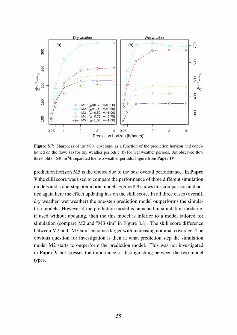
100
150
200
250
300
0.25 1 2 3 4
δ h(0.1
) [m3 /h
]Dry weather
M1 : (γ1=0.50 , γ2=0.50)M2 : (γ1=1.00 , γ2=0.50)M3 : (γ1=0.50 , γ2=1.00)M4 : (γ1=0.75 , γ2=0.75)M5 : (γ1=1.00 , γ2=1.00)
(a)
300
400
500
600
700
0.25 1 2 3 4
δ h(0.1
) [m3 /h
]
Wet weather
(b)
Prediction horizon [h(hours)]
Figure 8.7: Sharpness of the 90% coverage, as a function of the prediction horizon and condi-tioned on the flow: (a) for dry weather periods ; (b) for wet weather periods. An observed flowthreshold of 540 m3/h separated the two weather periods. Figure from Paper IV.
prediction horizon M5 is the choice due to the best overall performance. In PaperV the skill score was used to compare the performance of three different simulationmodels and a one-step prediction model. Figure 8.8 shows this comparison and no-tice again here the effect updating has on the skill score. In all three cases (overall,dry weather, wet weather) the one-step prediction model outperforms the simula-tion models. However if the prediction model is launched in simulation mode i.e.if used without updating, then the this model is inferior to a model tailored forsimulation (compare M2 and "M3 sim" in Figure 8.8). The skill score differencebetween M2 and "M3 sim" becomes larger with increasing nominal coverage. Theobvious question for investigation is then at what prediction step the simulationmodel M2 starts to outperform the prediction model. This was not investigatedin Paper V but stresses the importance of distinguishing between the two modeltypes.
55
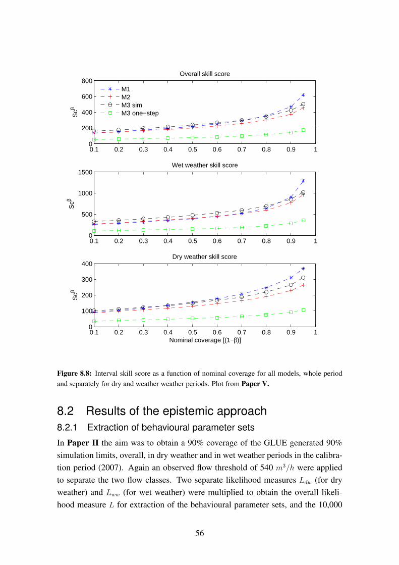
0.1 0.2 0.3 0.4 0.5 0.6 0.7 0.8 0.9 10
200
400
600
800Overall skill score
Scβ
M1M2M3 simM3 one−step
0.1 0.2 0.3 0.4 0.5 0.6 0.7 0.8 0.9 10
500
1000
1500Wet weather skill score
Scβ
0.1 0.2 0.3 0.4 0.5 0.6 0.7 0.8 0.9 10
100
200
300
400Dry weather skill score
Nominal coverage [(1−β)]
Scβ
Figure 8.8: Interval skill score as a function of nominal coverage for all models, whole periodand separately for dry and weather weather periods. Plot from Paper V.
8.2 Results of the epistemic approach8.2.1 Extraction of behavioural parameter sets
In Paper II the aim was to obtain a 90% coverage of the GLUE generated 90%simulation limits, overall, in dry weather and in wet weather periods in the calibra-tion period (2007). Again an observed flow threshold of 540 m3/h were appliedto separate the two flow classes. Two separate likelihood measures Ldw (for dryweather) and Lww (for wet weather) were multiplied to obtain the overall likeli-hood measure L for extraction of the behavioural parameter sets, and the 10,000
56
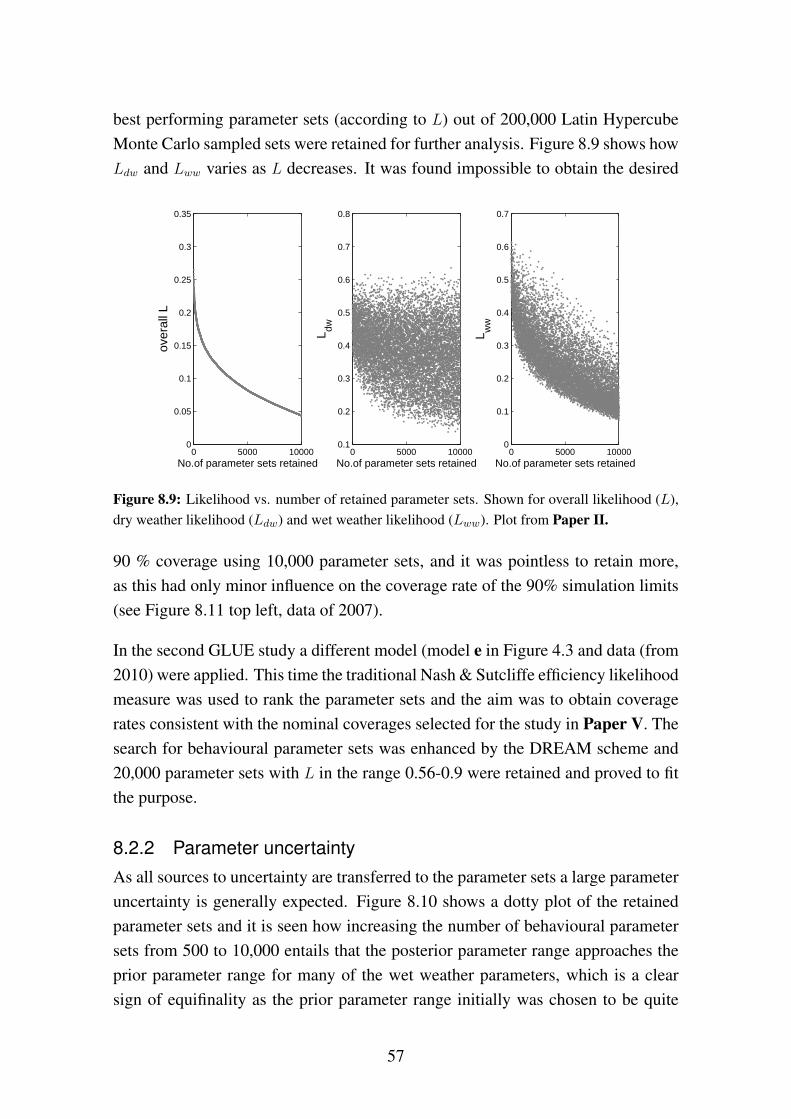
best performing parameter sets (according to L) out of 200,000 Latin HypercubeMonte Carlo sampled sets were retained for further analysis. Figure 8.9 shows howLdw and Lww varies as L decreases. It was found impossible to obtain the desired
0 5000 100000
0.05
0.1
0.15
0.2
0.25
0.3
0.35
over
all L
No.of parameter sets retained0 5000 10000
0.1
0.2
0.3
0.4
0.5
0.6
0.7
0.8
L dw
No.of parameter sets retained0 5000 10000
0
0.1
0.2
0.3
0.4
0.5
0.6
0.7
L ww
No.of parameter sets retained
Figure 8.9: Likelihood vs. number of retained parameter sets. Shown for overall likelihood (L),dry weather likelihood (Ldw) and wet weather likelihood (Lww). Plot from Paper II.
90 % coverage using 10,000 parameter sets, and it was pointless to retain more,as this had only minor influence on the coverage rate of the 90% simulation limits(see Figure 8.11 top left, data of 2007).
In the second GLUE study a different model (model e in Figure 4.3 and data (from2010) were applied. This time the traditional Nash & Sutcliffe efficiency likelihoodmeasure was used to rank the parameter sets and the aim was to obtain coveragerates consistent with the nominal coverages selected for the study in Paper V. Thesearch for behavioural parameter sets was enhanced by the DREAM scheme and20,000 parameter sets with L in the range 0.56-0.9 were retained and proved to fitthe purpose.
8.2.2 Parameter uncertaintyAs all sources to uncertainty are transferred to the parameter sets a large parameteruncertainty is generally expected. Figure 8.10 shows a dotty plot of the retainedparameter sets and it is seen how increasing the number of behavioural parametersets from 500 to 10,000 entails that the posterior parameter range approaches theprior parameter range for many of the wet weather parameters, which is a clearsign of equifinality as the prior parameter range initially was chosen to be quite
57
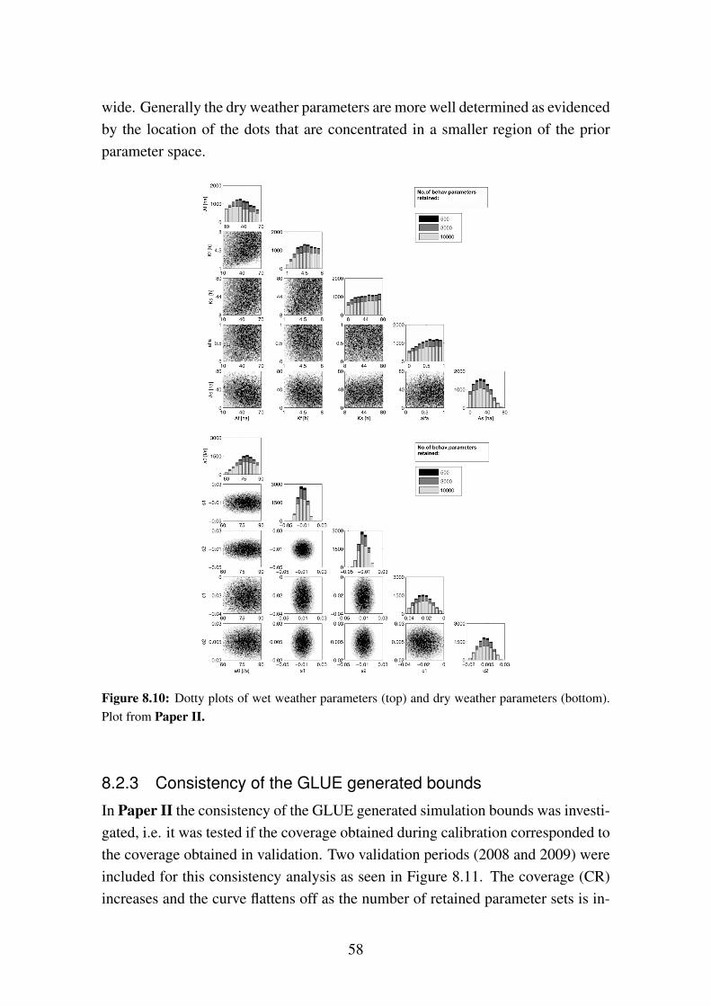
wide. Generally the dry weather parameters are more well determined as evidencedby the location of the dots that are concentrated in a smaller region of the priorparameter space.
Figure 8.10: Dotty plots of wet weather parameters (top) and dry weather parameters (bottom).Plot from Paper II.
8.2.3 Consistency of the GLUE generated bounds
In Paper II the consistency of the GLUE generated simulation bounds was investi-gated, i.e. it was tested if the coverage obtained during calibration corresponded tothe coverage obtained in validation. Two validation periods (2008 and 2009) wereincluded for this consistency analysis as seen in Figure 8.11. The coverage (CR)increases and the curve flattens off as the number of retained parameter sets is in-
58
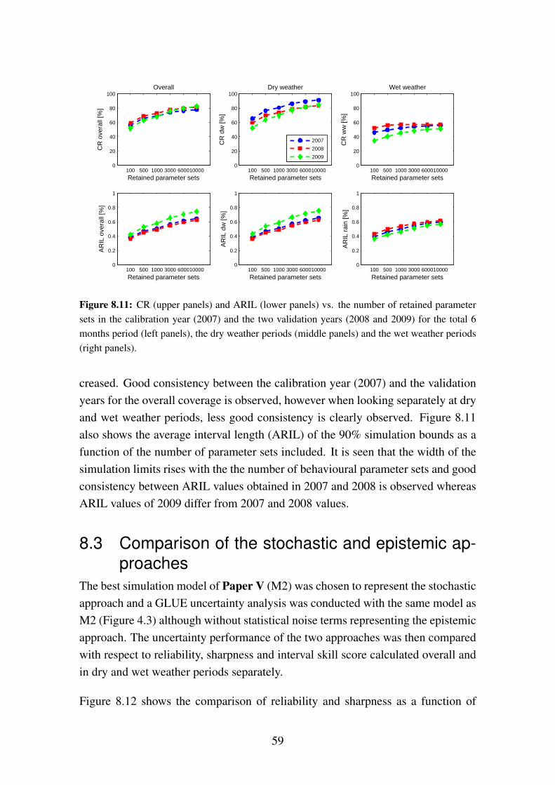
100 500 1000 3000 600010000 0
20
40
60
80
100
Retained parameter sets
CR
ove
rall
[%]
Overall
100 500 1000 3000 600010000 0
20
40
60
80
100
CR
dw
[%]
Dry weather
Retained parameter sets100 500 1000 3000 600010000
0
20
40
60
80
100
CR
ww
[%]
Retained parameter sets
Wet weather
100 500 1000 3000 600010000 0
0.2
0.4
0.6
0.8
1
AR
IL o
vera
ll [%
]
Retained parameter sets100 500 1000 3000 600010000
0
0.2
0.4
0.6
0.8
1
AR
IL d
w [%
]
Retained parameter sets100 500 1000 3000 600010000
0
0.2
0.4
0.6
0.8
1
AR
IL r
ain
[%]
Retained parameter sets
2007
2008
2009
Figure 8.11: CR (upper panels) and ARIL (lower panels) vs. the number of retained parametersets in the calibration year (2007) and the two validation years (2008 and 2009) for the total 6months period (left panels), the dry weather periods (middle panels) and the wet weather periods(right panels).
creased. Good consistency between the calibration year (2007) and the validationyears for the overall coverage is observed, however when looking separately at dryand wet weather periods, less good consistency is clearly observed. Figure 8.11also shows the average interval length (ARIL) of the 90% simulation bounds as afunction of the number of parameter sets included. It is seen that the width of thesimulation limits rises with the the number of behavioural parameter sets and goodconsistency between ARIL values obtained in 2007 and 2008 is observed whereasARIL values of 2009 differ from 2007 and 2008 values.
8.3 Comparison of the stochastic and epistemic ap-proaches
The best simulation model of Paper V (M2) was chosen to represent the stochasticapproach and a GLUE uncertainty analysis was conducted with the same model asM2 (Figure 4.3) although without statistical noise terms representing the epistemicapproach. The uncertainty performance of the two approaches was then comparedwith respect to reliability, sharpness and interval skill score calculated overall andin dry and wet weather periods separately.
Figure 8.12 shows the comparison of reliability and sharpness as a function of
59
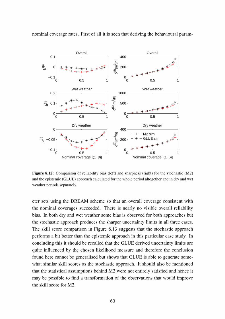
nominal coverage rates. First of all it is seen that deriving the behavioural param-
0 0.5 1−0.1
0
0.1
b(β)
Overall
0 0.5 10
0.1
0.2
b(β)
Wet weather
0 0.5 1−0.1
−0.05
0
Nominal coverage [(1−β)]
b(β)
Dry weather
0 0.5 10
200
400Overall
δ(β) [m
3 /h]
0 0.5 10
500
1000Wet weather
δ(β) [m
3 /h]
0 0.5 10
200
400Dry weather
Nominal coverage [(1−β)]
δ(β) [m
3 /h]
M2 simGLUE sim
Figure 8.12: Comparison of reliability bias (left) and sharpness (right) for the stochastic (M2)and the epistemic (GLUE) approach calculated for the whole period altogether and in dry and wetweather periods separately.
eter sets using the DREAM scheme so that an overall coverage consistent withthe nominal coverages succeeded. There is nearly no visible overall reliabilitybias. In both dry and wet weather some bias is observed for both approaches butthe stochastic approach produces the sharper uncertainty limits in all three cases.The skill score comparison in Figure 8.13 suggests that the stochastic approachperforms a bit better than the epistemic approach in this particular case study. Inconcluding this it should be recalled that the GLUE derived uncertainty limits arequite influenced by the chosen likelihood measure and therefore the conclusionfound here cannot be generalised but shows that GLUE is able to generate some-what similar skill scores as the stochastic approach. It should also be mentionedthat the statistical assumptions behind M2 were not entirely satisfied and hence itmay be possible to find a transformation of the observations that would improvethe skill score for M2.
60
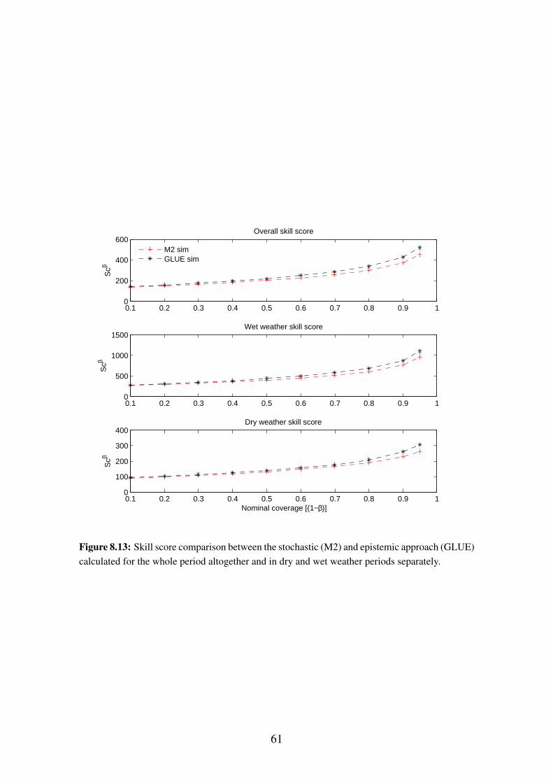
0.1 0.2 0.3 0.4 0.5 0.6 0.7 0.8 0.9 10
200
400
600Overall skill score
Scβ
M2 simGLUE sim
0.1 0.2 0.3 0.4 0.5 0.6 0.7 0.8 0.9 10
500
1000
1500Wet weather skill score
Scβ
0.1 0.2 0.3 0.4 0.5 0.6 0.7 0.8 0.9 10
100
200
300
400Dry weather skill score
Nominal coverage [(1−β)]
Scβ
Figure 8.13: Skill score comparison between the stochastic (M2) and epistemic approach (GLUE)calculated for the whole period altogether and in dry and wet weather periods separately.
61
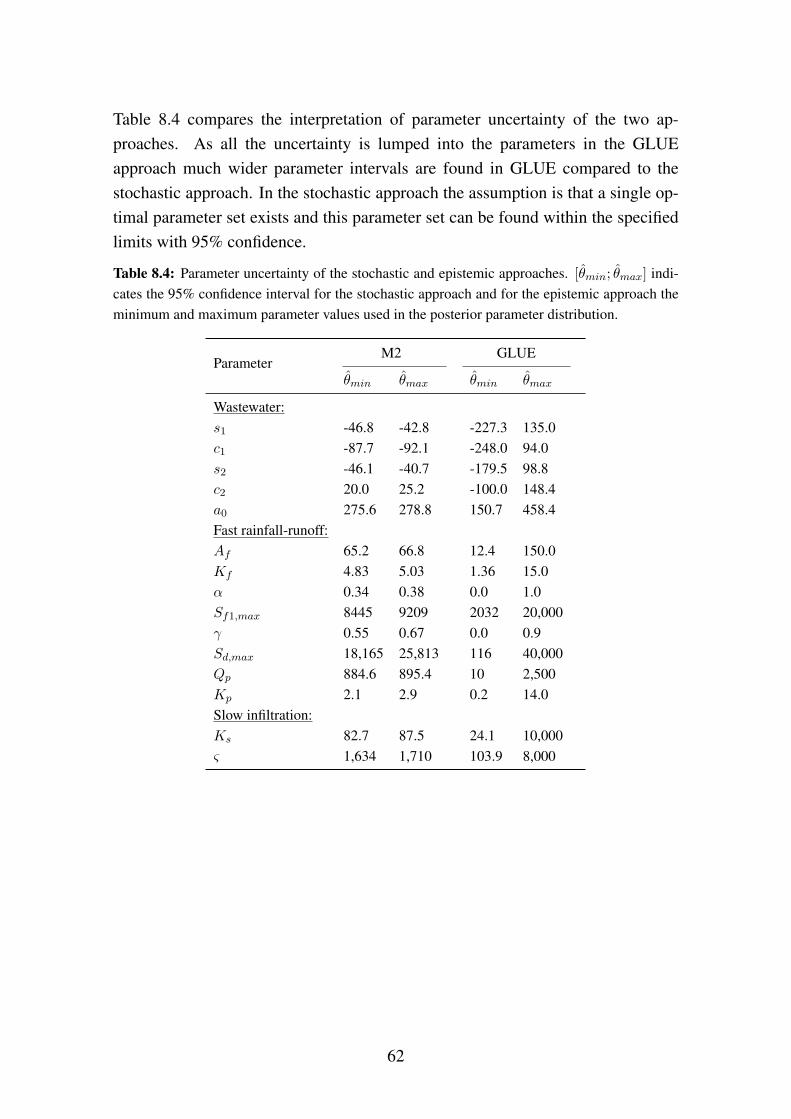
Table 8.4 compares the interpretation of parameter uncertainty of the two ap-proaches. As all the uncertainty is lumped into the parameters in the GLUEapproach much wider parameter intervals are found in GLUE compared to thestochastic approach. In the stochastic approach the assumption is that a single op-timal parameter set exists and this parameter set can be found within the specifiedlimits with 95% confidence.
Table 8.4: Parameter uncertainty of the stochastic and epistemic approaches. [θmin; θmax] indi-cates the 95% confidence interval for the stochastic approach and for the epistemic approach theminimum and maximum parameter values used in the posterior parameter distribution.
ParameterM2 GLUE
θmin θmax θmin θmax
Wastewater:s1 -46.8 -42.8 -227.3 135.0c1 -87.7 -92.1 -248.0 94.0s2 -46.1 -40.7 -179.5 98.8c2 20.0 25.2 -100.0 148.4a0 275.6 278.8 150.7 458.4Fast rainfall-runoff:Af 65.2 66.8 12.4 150.0Kf 4.83 5.03 1.36 15.0α 0.34 0.38 0.0 1.0Sf1,max 8445 9209 2032 20,000γ 0.55 0.67 0.0 0.9Sd,max 18,165 25,813 116 40,000Qp 884.6 895.4 10 2,500Kp 2.1 2.9 0.2 14.0Slow infiltration:Ks 82.7 87.5 24.1 10,000ς 1,634 1,710 103.9 8,000
62
9 ConclusionsThis main objective of this thesis has been to qualify and quantify output uncer-tainty in simulation and prediction using simple rainfall-runoff models for urbandrainage systems because such models are attractive for control purposes and be-cause uncertainty plays a significant role in the choice of an optimal control strat-egy. To assess the prediction and simulation uncertainty in a realistic setting acase catchment with real flow data was needed. The catchment of Ballerup waschosen and inputs included data from point rain gauges and monthly evaporationdata. Flow data sampled downstream from the catchment were used for modelconditioning and uncertainty evaluation. The data period covered 2007-2010. The1,320 ha catchment consists of both separated and combined sewage pipes, is sig-nificantly affected by infiltration inflow and facilitates a few detention basins andsome pumping stations.
To quantify the model output uncertainty two uncertainty approaches were distin-guished, the stochastic and the epistemic approach. A frequentist approach wastaken for the stochastic approach and the Generalised Likelihood Uncertainty Esti-mation (GLUE) methodology was adopted for the epistemic approach. Both meth-ods were applied for assessing the simulation uncertainty but only the stochasticapproach was applied for making predictions from continuous updating of modelstates.
Model developmentThe simple serial linear reservoir flow routing principle was applied for modellingboth the fast rainfall runoff from paved areas and the slow infiltration inflow frompermeable areas. The wastewater flow variation was modelled by a harmonic func-tion. Models of different complexity in terms of describing features such as flowconstraints, basins and pumps were tested for their ability to describe the outputwith a time resolution of 15 minutes.
The stochastic grey-box approach for predictionThe stochastic grey-box modelling approach that incorporates only the most impor-tant physical knowledge in the models and uses information from data to describethe uncertainty and for estimating the model parameters was chosen. Uncertainty isaccounted for explicitly by two noise terms, the observation noise term and the dif-fusion noise term. The parameters are estimated using the prediction error methodby maximising a likelihood function. All the estimated model parameters weretested for significance by a t-test and although most of the parameters could be de-
63
termined, some had to be fixed. Increasing the model complexity generally impliedthat more parameters had to be fixed. A flow proportional observation noise termwas preferred to an additive observation noise term because the flow metre accu-racy generally decreased with the flow magnitude and because the risk of receivingnegative flows is avoided. A state dependent diffusion term was also preferred to anadditive noise term because the risk of obtaining negative states could thereby beavoided. The state dependent diffusion term that was implemented by a Lampertitransformation of the states is also justified by the fact that the flow uncertaintygenerally increases with the volume of the rain. The residual tests contributed todeveloping the observation and diffusion noise terms and for the eventual approvalof the models. The Akaikes information criterion (AIC) and the Bayesian infor-mation criterion (BIC) were applied to choose a preferred model among the modelcandidates when considering the one-step prediction performance corresponding to15 minutes lead time, and the two criteria agreed well. In general the models wereunsuitable for making probabilistic forecasts beyond the one-step especially duringwet weather periods. For the case when a longer prediction horizon is required askill scoring criterion was applied to select a preferred model out of several modelcandidates. Even though a preferred model can be pinpointed from this criterion itshould be recognised that the model do not necessarily provide reliable forecasts.Therefore the sharpness and the reliability bias that evaluates the difference be-tween the nominal and observed coverage of a particular quantile were also usedto compare the models.
The stochastic approach for simulationIn the case that real time data are unavailable for continuous updating of the modelstates a simulation model can be applied instead. Assuming flow data from a mea-suring campaign are available for calibration it is possible to estimate the param-eters by maximum likelihood estimation and estimate the total output uncertainty.The parameter estimation can be conducted in two ways, either using the predic-tion error method (as discussed above) or by minimising the total output error forthe whole calibration period. In the latter case the diffusion term is removed andonly the observation noise term is kept. Three different models were tested. Two ofthe models contained only an observation noise term, one which was additive andone which was logistic, whereas the last one contained both an observation noiseterm and a diffusion noise term. Parameters were generally significant although afew parameters had to be fixed. In order to remove the heteroschedastic residualsstructure it was necessary to apply a logistic transformation of the observations,
64
however auto-correlation remained. The simulation model with a diffusion termembedded did not remove the auto-correlation either and hence it seems unrealisticto assume residual independency in the simulation case. The logistic observationnoise term improved the reliability of the confidence bounds significantly com-pared to an additive observation noise term. This model also proved to be the mostreliable simulation model and the skill scoring criterion pointed to this model asthe preferred model of the three simulation models. The reliability of the preferredmodels confidence bounds were similar in dry and wet weather periods. A skillscoring comparison of a simulation and a prediction model showed that a majorimprovement is gained by updating the model states continuously, i.e. updating ofmodel states results in much lower uncertainty.
The epistemic approach for simulationThe GLUE methodology is very different from the chosen stochastic approachbecause of the absent requirements to the residuals and because parameters areseen as stochastic variables. Nevertheless the aim is the same, namely to covera proportion of observations consistent with the considered quantile with maxi-mum sharpness. Two different likelihood measures were applied for qualifying themodel parameters, the traditional Nash & Suttcliffe model efficiency coefficientand an exponential variant. For sampling the model space a latin hypercube montecarlo method (LHS) and a markov chain monte carlo method (DREAM) were bothapplied. The algorithm in DREAM is very efficient in locating the high perform-ing areas of the model space and the posterior density ratio had to be adjusted tosecure visits of lower performing areas. Generally the use of DREAM saves com-putational time. To select the behavioral parameter sets a coverage criterion of90% by the generated 90% uncertainty limits was proposed. It was however im-possible to reach such a high coverage in the calibration period and the coveragewere much lower during rain than in dry weather. The consistency of the GLUEgenerated uncertainty limits were then evaluated by comparing obtained coveragerates between the calibration period and two validation periods and a reasonableconsistency was generally found.
Comparison of the stochastic and epistemic approach for simulationTo facilitate a comparison of the two approaches to uncertainty evaluation thesharpness, reliability and skill score were calculated for both using the same dataset for calibration and evaluation. Results showed that very similar performancewas obtained, with the stochastic method as the preferred. It should be stressed that
65
in order to test this more properly a data set other than the calibration data shouldbe used for validation. The work of this thesis has demonstrated that the statisticalrequirements to the formal stochastic approach, i.e. that residuals should conformto a white noise process, are very hard to fulfill in practice, especially in simulationand for predictions beyond one step where significant auto-correlation remained.The requirements were easier to fulfill for the one-step prediction which was due tothe continuous updating of the model states. As a consequence hereof the reliabil-ity of prediction steps beyond the one-step prediction was quite biased, especiallyduring rain. Although the GLUE derived uncertainty limits did not prove com-pletely consistent nor superior to the stochastic derived uncertainty description,the underlying assumption of the GLUE methodology that uncertainty in model-ing and simulation is not only of stochastic nature seems fairly consistent with theresults of this thesis. A major drawback of the GLUE methodology is the lumpingof total uncertainty into the parameters which entails a loss of physicality of themodel parameters. Conversely the parameter estimates of the stochastic approachare physically meaningful. This thesis has contributed to developing simplifiedrainfall-runoff models that are suitable for stochastic model predictive control ofurban drainage systems.
66
10 OutlookThe benchmarking tools and the grey box models developed in connection withthis thesis may well be applied to other catchments for assessing the uncertaintyon model outputs in connection with model predictive control investigations. Themodelled output are in that case not limited to flow forecasting but could just aswell be applied for forecasting of water level, volume or concentrations.
It should also be mentioned that measurements from levels of storage tanks orpumping stations could be directly used in the observation equation of the greybox model which would be desirable in many cases for improving the predictionperformance if such measurements are available.
The predictions made in connection with this thesis all assumed future rain inputsto be known. However because of the retention time of the system, i.e. betweena rainfall is recorded at the rain gauges until a corresponding runoff is observedat the flow meter in the sewer system, it is often possible to obtain a flow forecastwithout the need for rainfall input forecasts. This potential should be investigatedfurther.
As it was shown that a simulation model was more reliable than a prediction model(estimated by minimsing the one step ahead errors) when considering several pre-diction steps into the future it would be desirable to know up to which predictionstep we should apply the prediction model and hence at what prediction step thesimulation model becomes the preferred model. The skill score benchmaring tooloutlined in this thesis can be used for this investigation.
It was also shown that if the reliability were calculated separately for dry and wetweather periods, the reliability in dry weather periods (with reliability biases in theorder of 5% at prediction steps up to 4 hours) were generally higher than in wetweather periods in which a rapidly deteriorating reliability as a function of predic-tion horizon was found (with reliability biases in the order of 50-80% at 4 hourprediction steps). These findings suggest that the models predictive performancesfor prediction steps larger than one needs to be improved, and one way could per-haps be to replace the minimisation of the one step prediction error in the extendedKalman filter with a k step error minimisation in accordance with whatever leadtime is required for the desired model predictive control implementation.
It is in connection with model predictive control of a waste water treatment plantperhaps more important to predict the volume load to the plant over the next half
67

hour and in that case a grey box model optimised for this might perform better thana model optimised for predicting the inflow with 15 minutes time steps.
The use of rain radars to extend the lead time and obtain a more adequate spatio-temporal rain input description also holds a significant flow prediction potentialand the use of the performance indicators outlined in this thesis could be used toconclude on this potential.
Finally the next step should be to show how the probabilistic forecasts can beutilised in model predictive control.
68
11 ReferencesAchleitner, S., Fach, S., Einfalt, T., Rauch, W., 2009. Nowcasting of rainfall and of combined
sewage flow in urban drainage systems. Water Science & Technology - WST 59 (6), 1145–1151.
Andréassian, V., Lerat, J., Loumagne, C., Mathevet, T., Michel, C., Oudin, L., Perrin, C., 2007.What is really undermining hydrologic science today? Hydrological Processes 21 (20), 2819–2822.
Baadsgaard, M., Nielsen, J. N., Spliid, H., Madsen, H., Preisel, M., 1997. Estimation in stochasticdifferential equations with a state dependent diffusion term. SYSID ’97 - 11th IFAC symposiumof system identification, IFAC.
Beven, K., 2006. A manifesto for the equifinality thesis. Journal of Hydrology 320 (1-2), 18–36.
Beven, K., 2009a. Environmental modelling: An uncertain future / An introduction to techniquesfor uncertainty estimation in environmental prediction. Routledge Taylor & Francis Group.
Beven, K. J., 2009b. Comment on "Equifinality of formal (DREAM) and informal (GLUE)Bayesian approaches in hydrologic modeling?" by Jasper A. Vrugt, Cajo J. F. ter Braak, HoshinV. Gupta and Bruce A. Robinson. Stochastic Environmental Research and Risk Assessment23 (7), 1059–1060.
Beven, K. J., 2012. Rainfall - runoff modelling / The primer. John Wiley & Sons.
Beven, K., Binley, A., 1992. The future of distributed models - model calibration and uncertaintyprediction. Hydrological Processes 6 (3), 279–298.
Beven, K., Freer, J., 2001. Equifinality, data assimilation, and uncertainty estimation in mecha-nistic modelling of complex environmental systems using the GLUE methodology. Journal ofHydrology 249 (1-4), 11–29.
Beven, K., Smith, P., Freer, J., 2007. Comment on "Hydrological forecasting uncertainty assess-ment: Incoherence of the GLUE methodology" by Pietro Mantovan and Ezio Todini. Journal ofHydrology 338 (3-4), 315–318.
Beven, K. J., Smith, P. J., Freer, J. E., 2008. So just why would a modeller choose to be incoherent?Journal of Hydrology 354 (1-4), 15–32.
Beven, K., Smith, P. J., Wood, A., 2011. On the colour and spin of epistemic error (and what wemight do about it). Hydrology and Earth System Sciences 15 (10), 3123.
Blasone, R.-S., Vrugt, J. A., Madsen, H., Rosbjerg, D., Robinson, B. A., Zyvoloski, G. A., 2008.Generalized likelihood uncertainty estimation (GLUE) using adaptive Markov Chain MonteCarlo sampling. Advances in Water Resources 31 (4), 630–648.
Box, G. E., Jenkins, G. M., Reinsel, G. C., 2008. Time series analysis / Forecasting and control.Wiley, wiley series in probability and statistics.
69
Bruen, M., Yang, J., 2006. Combined hydraulic and black-box models for flood forecasting inurban drainage systems. J. Hydrologic Eng. 11 (6), 589–596.
Carstensen, J., Nielsen, M. K., Strandbæk, H., 1998. Prediction of hydraulic load for urban stromcontrol of a municipal wwt plant. Water Science & Technology 37 (12), 363–370.
Choi, H. T., Beven, K., 2007. Multi-period and multi-criteria model conditioning to reduce predic-tion uncertainty in an application of topmodel within the glue framework. Journal of Hydrology332 (3-4), 316–336.
Clark, M. P., Kavetski, D., Fenicia, F., 2011. Pursuing the method of multiple working hypothesesfor hydrological modeling. WATER RESOURCES RESEARCH 47, –.
Coccia, G., Todini, E., Coccia, G., 2011. Recent developments in predictive uncertainty assess-ment based on the model conditional processor approach. Hydrology and Earth System Sci-ences 15 (10), 3253–3274.
Dorado, J., Rabuñal, J. R., Pazos, A., Rivero, D., Puertas, A. S. J., 2003. Prediction and modelingof the rainfall-runoff transformation of a typical urban basin using ann and gp. Applied ArtificialIntelligence 17, 329–343, DOI: 10.1080/08839510390198673.
Dotto, C., Deletic, A., Fletcher, T., 2009. Analysis of parameter uncertainty of a flow and qualitystormwater model. Water Science and Technology 60 (3), 717–725.
Dotto, C., Kleidorfer, M., Deletic, A., Rauch, W., McCarthy, D., Fletcher, T., 2011. Performanceand sensitivity analysis of stormwater models using a bayesian approach and long-term highresolution data. Environmental Modelling and Software 26 (10), 1225–1239.
Engeland, K., Renard, B., Steinsland, I., Kolberg, S., 2010. Evaluation of statistical models forforecast errors from the hbv model. Journal of Hydrology - Amsterdam 384 (2-2), 142.
Engeland, K., Xu, C.-Y., Gottschalk, L., 2005. Assessing uncertainties in a conceptual water bal-ance model using bayesian methodology. Hydrological Sciences Journal - Journal des SciencesHydrologiques 50 (1), 45.
Franz, K., Hogue, T., 2011. Evaluating uncertainty estimates in hydrologic models: Borrow-ing measures from the forecast verification community. Hydrology and Earth System Sciences15 (11), 3367–3382.
Freer, J., Beven, K., Ambroise, B., 1996. Bayesian estimation of uncertainty in runoff predictionand the value of data: An application of the GLUE approach. Water Resources Research 32 (7),2161–2173.
Freni, G., Mannina, G., Viviani, G., 2009a. Uncertainty in urban stormwater quality modelling:The influence of likelihood measure formulation in the GLUE methodology. Science of theTotal Environment 408 (1), 138–145.
Freni, G., Mannina, G., Viviani, G., 2009b. Urban runoff modelling uncertainty: Comparisonamong bayesian and pseudo-bayesian methods. Environmental Modelling and Software 24 (9),1100–1111.
70
Fu, G., Butler, D., Khu, S.-T., Sun, S., Khu, S.-T., 2011. Imprecise probabilistic evaluation ofsewer flooding in urban drainage systems using random set theory. Water Resources Research47 (2), W02534.
Gallagher, M., Doherty, J., 2007. Parameter estimation and uncertainty analysis for a watershedmodel. Environmental Modelling and Software 22 (7), 1000–1020.
Gneiting, T., Balabdaoui, F., Raftery, A. E., 2007. Probabilistic forecasts, calibration and sharp-ness. Journal of the Royal Statistical Society: Series B (Statistical Methodology) 69 (2), 243–268.
Gneiting, T., Raftery, A. E., 2007. Strictly proper scoring rules, prediction and estimation. Journalof the American Statistical Association 102 (477), 359–378.
Haario, H., Laine, M., Mira, A., Saksman, E., 2006. Dram: Efficient adaptive mcmc. Statisticsand Computing 16 (4), 339–354.
Hansen, L. S., Borup, M., Møller, A., Mikkelsen, P. S., 2011. Flow forecasting in urban drainagesystems using deterministic updating of water levels in distributed hydraulic models. 12th In-ternational Conference on Urban Drainage.
Hostache, R., Matgen, P., Montanari, A., Montanari, M., Hoffmann, L., Pfister, L., 2011. Propa-gation of uncertainties in coupled hydro-meteorological forecasting systems: A stochastic ap-proach for the assessment of the total predictive uncertainty. Atmospheric Research 100 (2-3),263–274.
Jin, X., Xu, C.-Y., Zhang, Q., Singh, V., 2010. Parameter and modeling uncertainty simulated byglue and a formal bayesian method for a conceptual hydrological model. Journal of Hydrology- Amsterdam 383 (4-4), 147.
Jørgensen, H. K., Rosenørn, S., Madsen, H., Mikkelsen, P. S., 1998. Quality control of rain dataused for urban runoff systems. Water Science and Technology 37 (11), 113–120.
Kavetski, D., Kuczera, G., Franks, S., 2006. Bayesian analysis of input uncertainty in hydrologicalmodeling: 2. application. WATER RESOURCES RESEARCH 42 (3), –.
Kloeden, P. E., Platen, E., 1999. Numerical Solution of Stochastic Differential Equations.Springer-Verlag.
Kristensen, N. R., Madsen, H., 2003. Continuous Time Stochastic Modeling - CTSM 2.3 - Math-ematics Guide. Technical Unversity of Denmark.
Kristensen, N. R., Madsen, H., Jørgensen, S. B., 2004a. A method for systematic improvement ofstochastic grey-box models. Computers and Chemical Engineering 28 (8), 1431–1449.
Kristensen, N. R., Madsen, H., Jørgensen, S. B., 2004b. Parameter estimation in stochastic grey-box models. Automatica 40 (2), 225–237.
Krueger, T., Freer, J., Quinton, J. N., Macleod, C. J. A., Bilotta, G. S., Brazier, R. E., Butler,P., Haygarth, P. M., 2010. Ensemble evaluation of hydrological model hypotheses. WATERRESOURCES RESEARCH 46, –.
71
Laloy, E., Fasbender, D., Bielders, C., 2010. Parameter optimization and uncertainty analysisfor plot-scale continuous modeling of runoff using a formal Bayesian approach. Journal ofHydrology 380 (1-2), 82–93.
Li, L., Xia, J., Xu, C.-Y., Singh, V., 2010. Evaluation of the subjective factors of the GLUE methodand comparison with the formal Bayesian method in uncertainty assessment of hydrologicalmodels. Journal of Hydrology - Amsterdam 390 (4-4), 210.
Lindblom, E., Ahlman, S., Mikkelsen, P., 2011. Uncertainty-based calibration and prediction witha stormwater surface accumulation-washoff model based on coverage of sampled zn, cu, pb andcd field data. Water Research 45 (13), 3823–3835.
Liu, Y., Freer, J., Beven, K., Matgen, P., 2009. Towards a limits of acceptability approach tothe calibration of hydrological models: Extending observation error. Journal of Hydrology -Amsterdam 367 (2-2), 93.
Madsen, H., 2008. Time Series Analysis. Chapman & Hall/CRC.
Madsen, H., Thyregod, P., 2011. Introduction to general and generalized linear models. CRCPress, texts in statistical science.
Mantovan, P., Todini, E., 2006. Hydrological forecasting uncertainty assessment: Incoherence ofthe GLUE methodology. Journal of Hydrology 330 (1-2), 368–381.
Mantovan, P., Todini, E., Martina, M. L. V., 2007. Reply to comment by Keith Beven, Paul Smithand Jim Freer on "Hydrological forecasting uncertainty assessment: Incoherence of the GLUEmethodology". Journal of Hydrology - Amsterdam 338 (3-4), 319.
Matott, L. S., Babendreier, J. E., Purucker, S. T., Matott, L. S., 2009. Evaluating uncertainty inintegrated environmental models: A review of concepts and tools. Water Resources Research45 (6), W06421.
McIntyre, N., Young, P., Orellana, B., Marshall, M., Reynolds, B., Wheater, H., 2011. Identifica-tion of nonlinearity in rainfall-flow response using data-based mechanistic modeling. WATERRESOURCES RESEARCH 47, –.
McMillan, H., Clark, M., 2009. Rainfall-runoff model calibration using informal likelihoodmeasures within a markov chain monte carlo sampling scheme. WATER RESOURCES RE-SEARCH 45, –.
Morawietz, M., Xu, C.-Y., Gottschalk, L., Tallaksen, L. M., 2011. Systematic evaluation of autore-gressive error models as post-processors for a probabilistic streamflow forecast system. Journalof Hydrology 407 (1-4), 58–72.
Peel, M. C., Blöschl, G., 2011. Hydrological modelling in a changing world. Progress in PhysicalGeography 35 (2), 249–261.
Refsgaard, J., 1997. Validation and intercomparison of different updating procedures for real-timeforecasting. Nordic Hydrology 28, 65–84.
72
Refsgaard, J. C., Højberg, A. L., van der Sluijs, J. P., Vanrolleghem, P. A., Vanrolleghem, P. A.,2007. Uncertainty in the environmental modelling process - a framework and guidance. Envi-ronmental Modelling and Software 22 (11), 1543–1556.
Renard, B., Kavetski, D., Kuczera, G., Thyer, M., Franks, S. W., 2010. W05521 Understandingpredictive uncertainty in hydrologic modeling: The challenge of identifying input and structuralerrors (doi 10.1029/2009WR008328). Water Resources Research 46 (5).
Romanowicz, R. J., Young, P. C., Beven, K. J., Pappenberger, F., 2008. A data based mechanisticapproach to nonlinear flood routing and adaptive flood level forecasting. Advances in WaterResources 31 (8), 1048–1056.
Schoups, G., van de Giesen, N. C., Savenije, H. H. G., 2009. Model complexity control for hy-drologic prediction (doi 10.1029/2008wr006836). Water Resources Research 45 (12).
Schoups, G., Vrugt, J. A., 2010. A formal likelihood function for parameter and predictive in-ference of hydrologic models with correlated, heteroscedastic, and non-gaussian errors. WaterResources Research 46 (10), W10531.
Schütze, M., Butler, D., Beck, M., 2002. Modelling, simulation and control of urban wastewatersystems. Springer-Verlag.
Stedinger, J. R., Vogel, R. M., Lee, S. U., Batchelder, R., 2008. Appraisal of the generalizedlikelihood uncertainty estimation (GLUE) method. Water Resources Rsearch 44, 1–17.
Taylor, C. J., Pedregal, D. J., Young, P. C., Tych, W., 2007. Environmental time series analysis andforecasting with the captain toolbox. Environmental Modelling and Software 22 (6), 797–814.
Thordarson, F. Ö., 2012. Grey box modelling of hydrological systems with focus on uncertainties.Ph.D. thesis, DTU Informatics, Technical University of Denmark.
Thorndahl, S., Beven, K., Jensen, J., Schaarup-Jensen, K., 2008. Event based uncertainty assess-ment in urban drainage modelling, applying the GLUE methodology. Journal of Hydrology357 (3-4), 421–437.
Thyer, M. A., Renard, B., Kavetski, D., Kuczera, G., Srikanthan, S., 2007. Bayesian total erroranalysis for hydrological models: Preliminary evaluation using multi-site catchment rainfalldata. MODSIM 2007: INTERNATIONAL CONGRESS ON MODELLING AND SIMULA-TION, 2459–2465.
Todini, E., 2007. Hydrological catchment modelling: past, present and future. Hydrology andEarth System Sciences 11 (1), 468.
Todini, E., 2011. History and perspectives of hydrological catchment modelling. Hydrology Re-search 42 (2-3), 73–85.
Tomicic, B., 2006. Kapacitetsplanlægning. Opdatering af MOUSE/MIKE URBAN Model. Mod-eltilpasningsrapport for spildevandscenter Avedøre. Tech. rep., Danish Hydraulic Institute(DHI), Hørsholm, Denmark.
73
Vestergaard, M., 1998. Nonlinear filtering in stochastic volatility models, Master Thesis. Techni-cal University of Denmark. Department of Mathematical Modelling, Lyngby, Denmark.
Vezzaro, L., Mikkelsen, P. S., 2012. Application of global sensitivity analysis and uncertaintyquantification in dynamic modelling of micropollutants in stormwater runoff. EnvironmentalModelling and Software 27-28, 40–51.
Vojinovic, Z., Kecman, V., Babovic, V., 2003. Hybrid approach for modeling wet weather re-sponse in wastewater systems. Journal of Water Resources Planning and Management 129 (6),511–521.
Vrugt, J. A., 2011. DREAM<sub>(D)</sub>: an adaptive markov chain monte carlo simulationalgorithm to solve discrete, noncontinuous, posterior parameter estimation problems. Hydrol-ogy and Earth System Sciences Discussions 8 (2), 4025.
Vrugt, J. A., Braak, C. J. F. t., Gupta, H. V., Robinson, B. A., 2009a. Equifinality of formal(DREAM) and informal (GLUE) Bayesian approaches in hydrologic modeling? StochasticEnvironmental Research and Risk Assessment 23 (7), 1011–1026.
Vrugt, J. A., ter Braak, C. J. F., Clark, M. P., Hyman, J. M., Robinson, B. A., 2009b. W00B09- Treatment of input uncertainty in hydrologic modeling: Doing hydrology backward withMarkov chain Monte Carlo simulation (DOI 10.1029/2007WR006720). Water Resources Re-search 45 (12).
Vrugt, J. A., ter Braak, C. J. F., Diks, C. G. H., Robinson, B. A., Hyman, J. M., Higdon, D.,2009c. Accelerating Markov Chain Monte Carlo Simulation by Differential Evolution withSelf-Adaptive Randomized Subspace Sampling. International Journal of Nonlinear Sciencesand Numerical Simulations 10 (3), 273.
Vrugt, J. A., ter Braak, C. J. F., Gupta, H. V., Robinson, B. A., 2009d. Response to comment byKeith Beven on "Equifinality of formal (DREAM) and informal (GLUE) Bayesian approachesin hydrologic modeling?". Stochastic Environmental Research and Risk Assessment 23 (7),1061–1062.
Walker, W., Harremoes, P., Rotmans, J., van der Sluijs, J., van Asselt, M., Janssen, P., von Krauss,M. K., 2005. Defining uncertainty: A conceptual basis for uncertainty management in model-based decision support. Integrated Assessment 4 (1).
Westerberg, I. K., Guerrero, J.-L., Younger, P. M., Beven, K. J., Seibert, J., Halldin, S., Freer, J. E.,Xu, C.-Y., 2010. Calibration of hydrological models using flow-duration curves. Hydrology andEarth System Sciences Discussions 7 (6), 9467.
Xiong, L., Wan, M., Wei, X., O’Connor, K. M., 2009. Indices for assessing the prediction boundsof hydrological models and application by generalised likelihood uncertainty estimation. Hy-drological Sciences Journal 54 (5), 852–871.
Yang, J., Reichert, P., Abbaspour, K., Xia, J., Yang, H., 2008. Comparing uncertainty analysistechniques for a swat application to the chaohe basin in china. Journal of Hydrology 358 (1-2),1–23.
74

Yang, J., Reichert, P., Abbaspour, K. C., Yang, H., 2007. Hydrological modelling of the ChaoheBasin in China: Statistical model formulation and Bayesian inference. Journal of Hydrology340 (3-4), 167–182.
Young, P., Garnier, H., 2006. Identification and estimation of continuous-time, data-based mech-anistic (DBM) models for environmental systems. Environmental Modelling and Software21 (8), 1055–1072.
Young, P. C., 2011. Gauss, Kalman and advances in recursive parameter estimation. Journal ofForecasting 30 (1), 104–146.
75

76
12 Papers
Paper I. Breinholt, A., Santacoloma, P.A., Mikkelsen, P.S., Madsen, H., Grum,M., Nielsen, M.K. Evaluation framework for control of integrated urban drainagesystems, In: 11ICUD, Proceedings of 11th International Conference on UrbanDrainage, Edinburgh, Scotland, 31st August-5th September 2008.
Paper II. Breinholt, A., Grum, M., Madsen, H. , Thordarson, F.Ø., Mikkelsen,P.S. Informal uncertainty analysis (GLUE) of continuous flow simulation ina hybrid sewer system with infiltration inflow - consistency of containmentratios in calibration and validation?, submitted.
Paper III. Breinholt, A., Thordarson, F.Ø., Møller, J.K., Grum, M., Mikkelsen,P.S., Madsen, H. Grey-box modelling of flow in sewer systems with state de-pendent diffusion, Environmetrics, Vol. 22 (8), pp. 946-961, 2011 (DOI:10.1002/env.1135).
Paper IV. Thordarson, F.Ø., Breinholt, A., Møller, J.K., Mikkelsen, P.S. Grum,M., Madsen, H. Evaluation of probabilistic flow predictions in sewer systemsusing grey box models and a skill score criterion. Stochastic EnvironmentalResearch and Risk Assessment.(in press)(DOI: 10.1007/s00477-012-0563-3).
Paper V. Breinholt, A., Møller, J.K., Madsen, H., Mikkelsen, P.S. A formal sta-tistical approach to representing uncertainty in rainfall-runoff modelling withfocus on residual analysis and probabilistic output evaluation - distinguishingsimulation and prediction, submitted.
Paper VI. Breinholt, A., Thordarson, F.Ø., Møller, J.K., Grum, M., Mikkelsen,P.S., Madsen, H. Identifying the appropriate physical complexity of stochasticgray-box models used for urban drainage flow prediction by evaluating theirpoint and probabilistic forecast skill, submitted.
The papers are not included in this www-version, but can be obtained from the Li-brary at DTU Environment: Department of Environmental Engineering TechnicalUniversity of Denmark Miljoevej, Building 113 2800 Kongens Lyngby, Denmark([email protected])
77


Technical University of Denmark
DTU Environment
Department of Environmental Engineering
Miljoevej, building 113
DK-2800 Kgs. Lyngby
Denmark
Phone: +45 4525 1600
Fax: +45 4593 2850
e-mail: [email protected]
www.env.dtu.dk
The Department of Environmental Engineering (DTU Environment) conducts
science-based engineering research within four themes:
Water Resource Engineering, Urban Water Engineering,
Residual Resource Engineering and Environmental Chemistry & Microbiology.
Each theme hosts two to four research groups.
The department dates back to 1865, when Ludvig August Colding, the
founder of the , gave the first lecture on sanitary engineering as
response to the cholera epidemics in Copenhagen in the late 1800s.
department
ISBN 978-87-92654-60-1