Uncertainty in Traffic Crash Reconstruction,Part 1: Bootstrapping from Small Samples

Jeremy S. Daily!

June 6, 2008

Quantities used in crash reconstruction often have inherent variation and a single value is notappropriate. A common way to overcome this deficiency is to use a range. This paper willpresent a technique, based on sampling statistics, to determine a distribution and subsequentrange in a logical and mathematically consistent fashion. If the parameter in question is nor-mally distributed, then the Student-t and !2 (chi-squared) distributions from sampling statisticsprovide descriptions of the mean and variance respectively. The number of samples determinethe characteristics of both the Student-t and !2 distributions. In a real world application, boththe mean and variance are unknown so simplifying assumptions found in statistics texts do notapply. In fact, compounding all the uncertainties leads to a larger precision interval than desired.Therefore, a stochastic equation is presented that requires numerical integration to obtain thefinal distribution of the parameter. The precision interval (range) obtained from this distributionrepresents the uncertainty associated with limited samples. As the number of samples increase,the resulting distribution approaches a normal distribution defined by the sample mean and sam-ple standard deviation. A numerical example demonstrates convergence. If too few data pointsare used, the results may give an unacceptably large range which suggests additional samplesare required. A traffic crash reconstruction related example is included.

Keywords Small sample sizes, bootstrapping, probability, traffic crash reconstruction, accident analysis

!Assistant Professor of Mechanical Engineering, The University of Tulsa, 800 S. Tucker Dr., Tulsa, OK 74104-3189, PH: (918)631-3056, e-mail: jeremy-daily@utulsa.edu

1

1 Introduction

1.1 Motivation

Many technical processes and problems have variation associated with them. This is especially true in thefield of traffic crash reconstruction or other forensic investigations where many of the data are obtainedthrough measurements that are subject to the ability of the investigator [1–5]. For example, the basic premiseof traffic crash reconstruction is to give an assessment of the state of the vehicles or parties involved beforethe crash based on measurable and anecdotal evidence from the crash scene. These measurements, whethertaken at the scene or sometime later, are only representative of the true or correct values for a particular crashevent. Some error1 exists with any measurement about the correct values so precision intervals, or ranges arecommonly used to represent the uncertainty. The goal of this paper is to provide a mathematically consistenttechnique for determining a precision interval based on limited data.For example, the drag factor of a certain vehicle/road system may be desired during the investigation of a

crash. To determine drag factor, an investigator uses an accelerometer in an exemplar vehicle on the samesurface of the crash to obtain the following measurements: 0.763, 0.720, 0.751, and 0.743. Notice that thesemeasurements have exceed the 5% spread which has commonly been taught as a criteria for “good” mea-surements in crash reconstruction [6]. The arithmetic mean of the samples is x̄ = 0.744; however, obtaininganother measurement may change the value of the estimated mean. The estimated standard deviation (ameasure of spread) for the above data is s = 0.0181. In a similar manner, the estimated standard deviationmay change with subsequent measurements, or, the actual value of the drag factor for the actual crash underinvestigation may be slightly lower or higher than the current measurements indicate.If only the mean value is of interest, a well established uncertainty analysis can be performed [7] using

the concept of the standard error. However, in a forensic context, all probable values must be considered.Therefore, the range must be estimated from the mean and standard deviation– both of which are unknown.For this situation, introductory texts on statistics do not address the procedure for estimating a precisioninterval when both parameters are unknown. Simply combining the 95% confidence interval for the meanwith the 95% confidence interval for the standard deviation will lead to an interval that is greater than 95%.Therefore, a bootstrapping (Monte Carlo based) approach is employed in this paper.A so-called good measurement must repeatably and accurately represent the phenomenon being measured

at reasonable cost. The reader should always ensure the data used in an investigation are being appliedcorrectly and no blunders are present in an analysis. The techniques presented herein assume the data arevalid and are being applied according to sound mathematical and physical principles [8].Statistical analysis does not turn erroneous data into valid data. Furthermore, only the data gathered are

being used. This means any prior knowledge is ignored. Other approaches exist, such as Bayesian analysis,that can include prior knowledge in an analysis as introduced by [9–12].

1Error is defined as the difference between the measured value of the variable and the true value of the variable and is necessarilyunknown.

2

1.2 Background

The technical aspect of this paper requires the reader to have a working understanding of statistics as outlinedin introductory texts [13]. However, a brief explanation of the statistical terms will be presented in thissection.The goal of this paper is to demonstrate a technique of obtaining estimates for the lower and upper bounds

of a range to use in subsequent deterministic calculations. The word deterministic means the values in anexpression are single valued. In other words, there is only one value for each variable. However, in astochastic problem, one or more variables can have multiple values, that is, the variable is random. Whenthis occurs, one must employ non-deterministic methods to perform the calculations.A stochastic variable can be classified into a few main groups. In general, a variable can be either discrete

or continuous. A discrete quantity is something that can be counted, like the number of vehicles travelingthrough an intersection, and a continuous quantity is something one measures; for example, length or accel-eration. This discussion will deal with continuous variables and using measurements to determine a range ofpossible values.There are two types of uncertainty associated with a variable as outlined by [14]. The first is type is called

aleatory uncertainty which describes the inherent variability associated with a particular quantity. This canbe thought of as the noise of the system. The second type of uncertainty is called epistemic uncertainty. Thisuncertainty is associated with lack of information. As the amount of information about a particular variableincreases, the epistemic uncertainty decreases. When estimating parameters with limited data, both aleatoryand epistemic uncertainty exist. Therefore, the approach presented herein represents both the aleatory andepistemic uncertainties.

1.3 Random Variables

Examples of random variables in traffic crash reconstruction include drag factor, pedestrian walking speeds,perception-response time, and distance measurements. Distance measurements are random,2 not because thelength is always changing, but because of different measuring techniques and the human error associated indetecting beginning and ending points. Clear examples of measurement variation common in traffic crash in-vestigation are demonstrated by [1,2]. Even if an event was recorded and a desired parameter was measured,there exists uncertainty inherent to the measurement process.Of the many ways to represent uncertainty, probability functions are widely adopted. If one has com-

plete knowledge of a continuous probability function, then probabilities can be assigned to certain intervals.Probability functions must adhere to the following axioms of probability [15]:

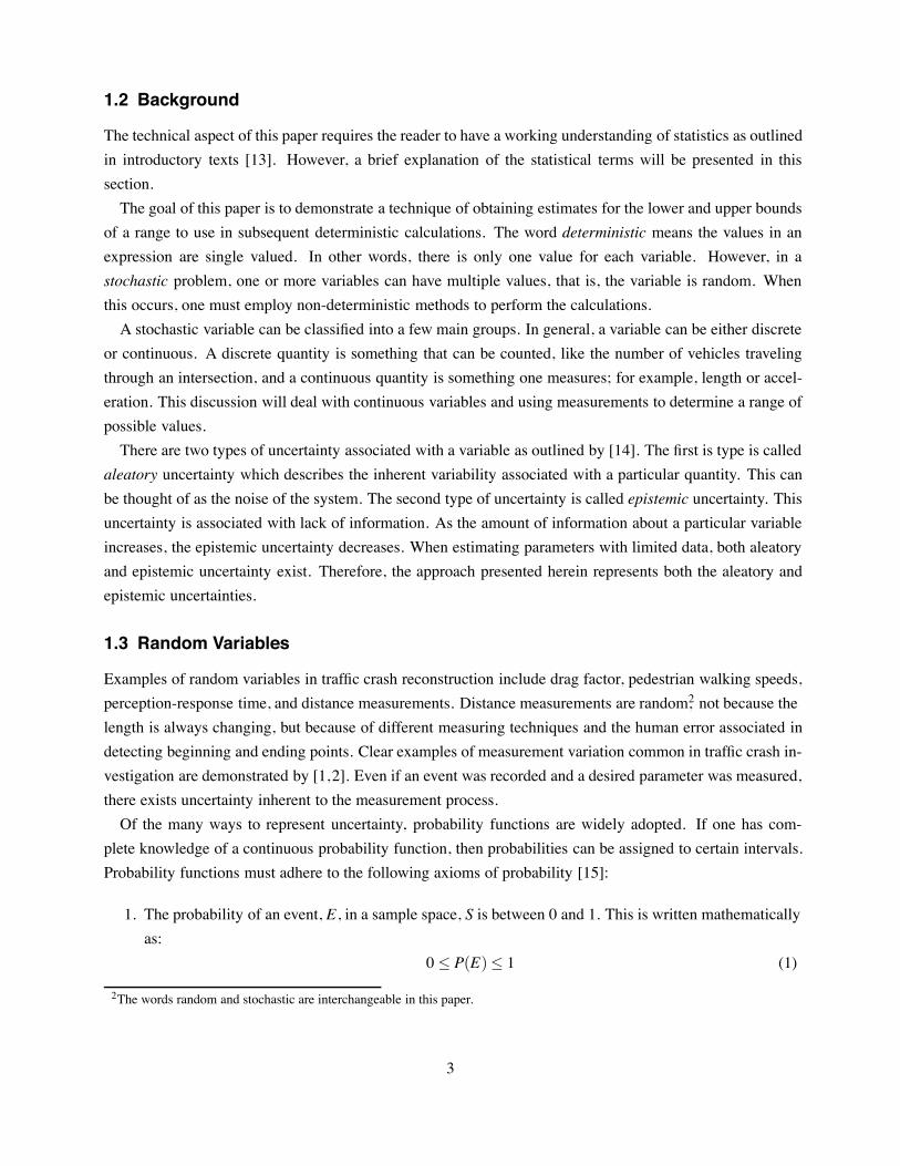
1. The probability of an event, E , in a sample space, S is between 0 and 1. This is written mathematicallyas:

0" P(E)" 1 (1)

2The words random and stochastic are interchangeable in this paper.

3

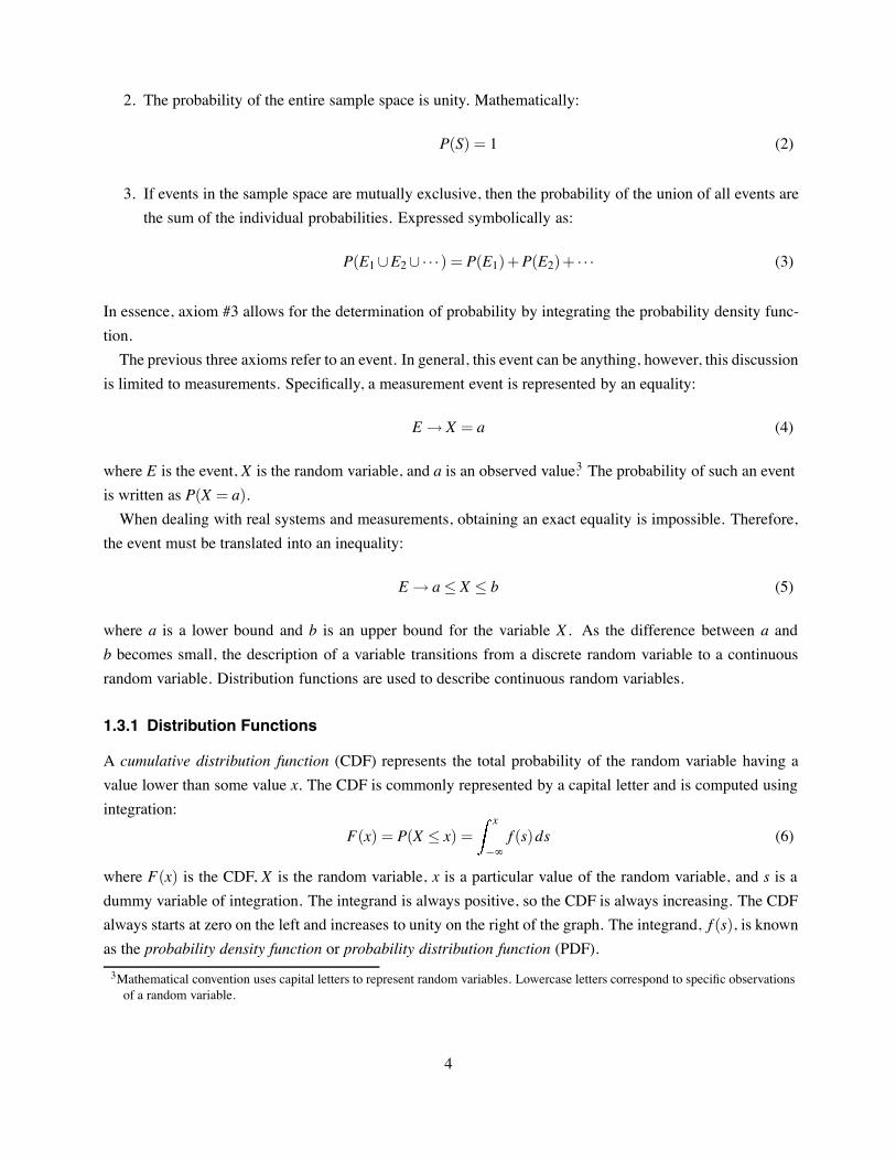
2. The probability of the entire sample space is unity. Mathematically:

P(S) = 1 (2)

3. If events in the sample space are mutually exclusive, then the probability of the union of all events arethe sum of the individual probabilities. Expressed symbolically as:

P(E1#E2# · · ·) = P(E1)+P(E2)+ · · · (3)

In essence, axiom #3 allows for the determination of probability by integrating the probability density func-tion.The previous three axioms refer to an event. In general, this event can be anything, however, this discussion

is limited to measurements. Specifically, a measurement event is represented by an equality:

E $ X = a (4)

where E is the event, X is the random variable, and a is an observed value.3 The probability of such an eventis written as P(X = a).When dealing with real systems and measurements, obtaining an exact equality is impossible. Therefore,

the event must be translated into an inequality:

E $ a" X " b (5)

where a is a lower bound and b is an upper bound for the variable X . As the difference between a andb becomes small, the description of a variable transitions from a discrete random variable to a continuousrandom variable. Distribution functions are used to describe continuous random variables.

1.3.1 Distribution Functions

A cumulative distribution function (CDF) represents the total probability of the random variable having avalue lower than some value x. The CDF is commonly represented by a capital letter and is computed usingintegration:

F(x) = P(X " x) =x

%"f (s)ds (6)

where F(x) is the CDF, X is the random variable, x is a particular value of the random variable, and s is adummy variable of integration. The integrand is always positive, so the CDF is always increasing. The CDFalways starts at zero on the left and increases to unity on the right of the graph. The integrand, f (s), is knownas the probability density function or probability distribution function (PDF).3Mathematical convention uses capital letters to represent random variables. Lowercase letters correspond to specific observationsof a random variable.

4

The PDF is the derivative of the CDF and commonly is represented by a lowercase letter:

f (x) =dF(x)dx

(7)

Once the PDF is known, the probability of any interval can be calculated using integration:

P(a" x" b) =b

af (x)dx (8)

Often, as is the case in this paper, the evaluation of the integral in Eq. (8) must be performed numerically.The Monte Carlo integration scheme [16] is widely popular as well as other advanced statistical samplingschemes [17]. Two common distribution functions used in crash reconstruction are the uniform and normaldistribution [18].The uniform distribution is the easiest distribution to use and also is the most “conservative” because it

gives an equal probability to all numbers within the distribution range. The formula for the PDF of a uniformdistribution from a to b.

fx(x) =

!"""#

"""$

0 x< a1

b%a a" x" b

0 x> b

(9)

Since the uniform distribution is so common, it is often written in shorthand asU(a,b) as shown in equation(9). The cumulative density function for the uniform distribution is

Fx(x) =

!"""#

"""$

0 x< a1

b%a(x%a) a" x" b

1 x> b

(10)

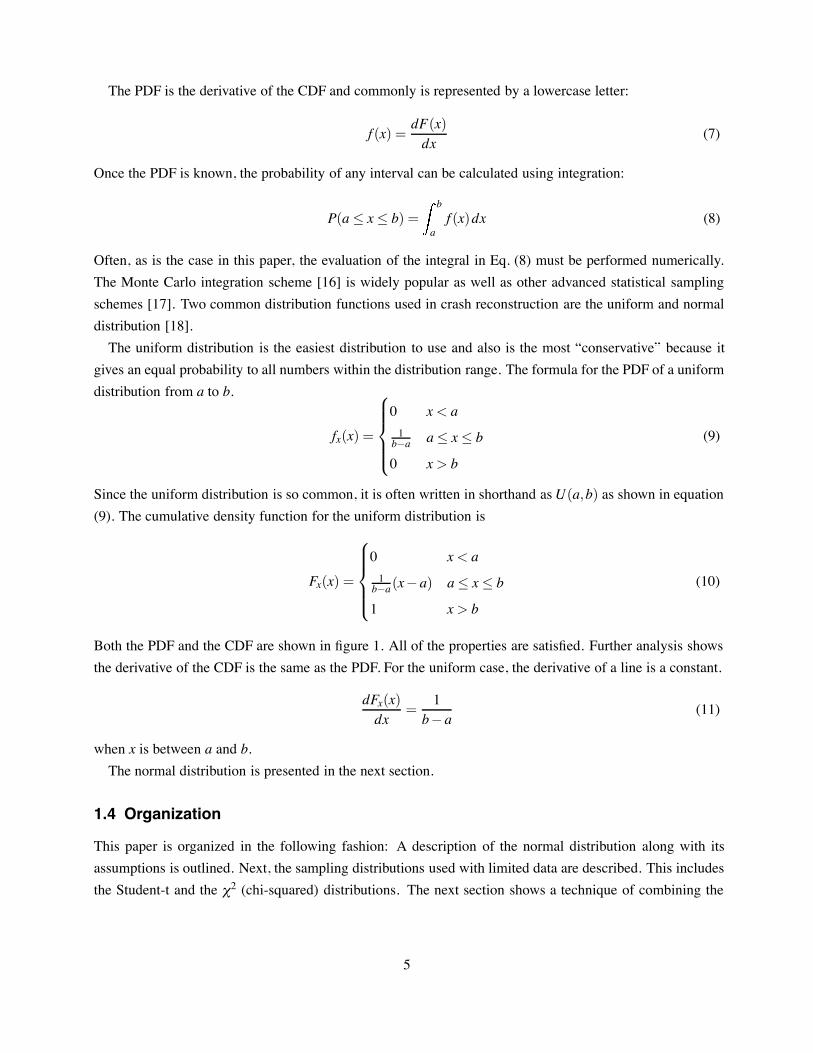
Both the PDF and the CDF are shown in figure 1. All of the properties are satisfied. Further analysis showsthe derivative of the CDF is the same as the PDF. For the uniform case, the derivative of a line is a constant.

dFx(x)dx

=1

b%a(11)

when x is between a and b.The normal distribution is presented in the next section.

1.4 Organization

This paper is organized in the following fashion: A description of the normal distribution along with itsassumptions is outlined. Next, the sampling distributions used with limited data are described. This includesthe Student-t and the !2 (chi-squared) distributions. The next section shows a technique of combining the

5

0.80.6f

area= P(value< x)

x

fx(x)

(a) Probability Density Function

0.80.6

1

0

P(value< x)

xX

ab%a

Fx(x)

(b) Cumulative Density Function

Figure 1: An example of the uniform distribution representing a range of drag factors where a = 0.6 andb= 0.8.

sampling distributions using Monte Carlo techniques to get an overall distribution and subsequent precisioninterval. This precision interval is the desired range, which is the main contribution of this paper. Finally, anumerical example showing the nature of convergence is presented.

2 The Normal Distribution

2.1 The Most Likely Distribution

Many times an analyst will have to assume a shape for a distribution. The normal distribution is the mostlikely distribution for an unknown naturally occurring quantity. Moreover, the techniques presented in thispaper are robust, meaning that if the underlying distribution is slightly non-normal, then the estimates pro-vided are still good. Gross deviation from normality does render the results meaningless and caution mustbe exercised to ensure the quantity under analysis is normal or near normal. This can be done visually bylooking to a straight line when plotting standard deviations or a more advanced statistical test such as theKolmogorov-Smirnov test [19].

2.2 Definition

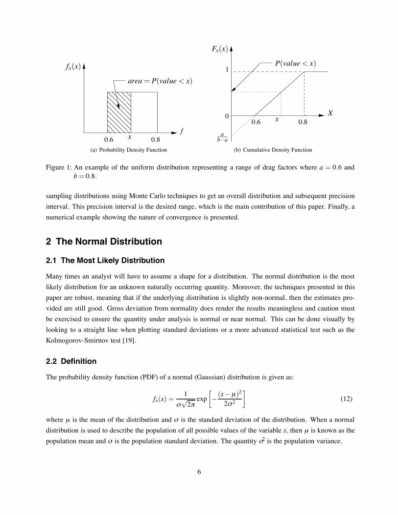
The probability density function (PDF) of a normal (Gaussian) distribution is given as:

fx(x) =1

#&2$exp

%%(x%µ)2

2#2

&(12)

where µ is the mean of the distribution and # is the standard deviation of the distribution. When a normaldistribution is used to describe the population of all possible values of the variable x, then µ is known as thepopulation mean and # is the population standard deviation. The quantity #2 is the population variance.

6

x

f (x)

µ

95% Precision Interval

(a) The PDF of a normal distribution

0

0.5

1.0

x

F(x)

µ

0.95

(b) The CDF of a normal distribution

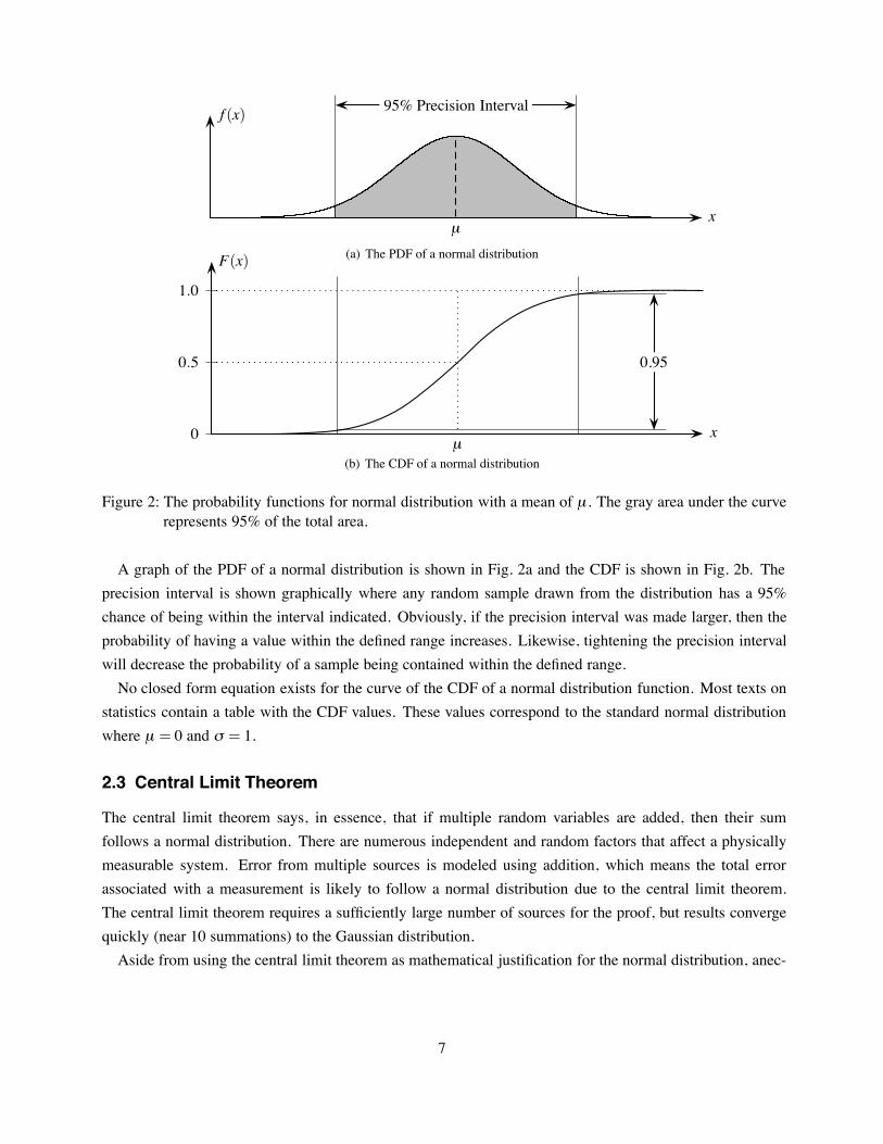
Figure 2: The probability functions for normal distribution with a mean of µ . The gray area under the curverepresents 95% of the total area.

A graph of the PDF of a normal distribution is shown in Fig. 2a and the CDF is shown in Fig. 2b. Theprecision interval is shown graphically where any random sample drawn from the distribution has a 95%chance of being within the interval indicated. Obviously, if the precision interval was made larger, then theprobability of having a value within the defined range increases. Likewise, tightening the precision intervalwill decrease the probability of a sample being contained within the defined range.No closed form equation exists for the curve of the CDF of a normal distribution function. Most texts on

statistics contain a table with the CDF values. These values correspond to the standard normal distributionwhere µ = 0 and # = 1.

2.3 Central Limit Theorem

The central limit theorem says, in essence, that if multiple random variables are added, then their sumfollows a normal distribution. There are numerous independent and random factors that affect a physicallymeasurable system. Error from multiple sources is modeled using addition, which means the total errorassociated with a measurement is likely to follow a normal distribution due to the central limit theorem.The central limit theorem requires a sufficiently large number of sources for the proof, but results convergequickly (near 10 summations) to the Gaussian distribution.Aside from using the central limit theorem as mathematical justification for the normal distribution, anec-

7

dotal evidence strongly suggests many physical and natural phenomena follow a classic “bell” curve whichis well represented by the normal distribution. That being said, the normality assumption of the underlyingdata should be examined for each variable under analysis.

3 Sampling Statistics

Assume a quantity follows a normal distribution and n samples are taken from that population. For example,an investigator conducts four drag factor tests (n = 4) and it is assumed that drag factor follows a normaldistribution. This normal distribution has an unknown mean and an unknown variance. From the n samples,one can obtain estimates of those parameters. Of the different estimators, the most common used are thearithmetic sample mean:

x̄= %ni=1 xin

(13)

and the sample variance:

s2 = %ni=1(xi% x̄)2

n%1 (14)

The sample standard deviation is the square root of the variance (s =&s2). These estimators are purely a

function of the gathered data. However, when making assertions about the quality of these estimates, thesample size is important.

3.1 Statistics of the mean

As the number of samples increases, the estimated mean, x̄, converges to the population mean. However,with a small number of samples, the estimated mean may be different than the population mean. A precisioninterval can be constructed around the sample mean that will include the actual population mean. Theconstruction of this precision interval is based on the Student-t distribution and the standard error (serr). Theformula for the standard error is

serr =s&n

(15)

The precision interval for the population mean utilized the Student-t distribution along with the sample sizeaccording to the following equation:

µ = x̄± t& ,'s&n

(16)

where t& ,' is a value from the Student-t distribution based on significance, & , and the degrees of freedom,' . The degrees of freedom, in a statistical sense, is the number of data points less the number of estimatedparameters. For example, if a data set of 9 points is fit with a quadratic curve (3 coefficients), then the numberof degrees of freedom is 6. Fir the t-test, only the mean has been determined, so ' = n%1. Notice in Eq. (16)as the number of samples increases, the standard error will decrease and the precision interval collapses ontothe true mean.

8

0 1 2 3 4%1%2%3%4x

f (x)

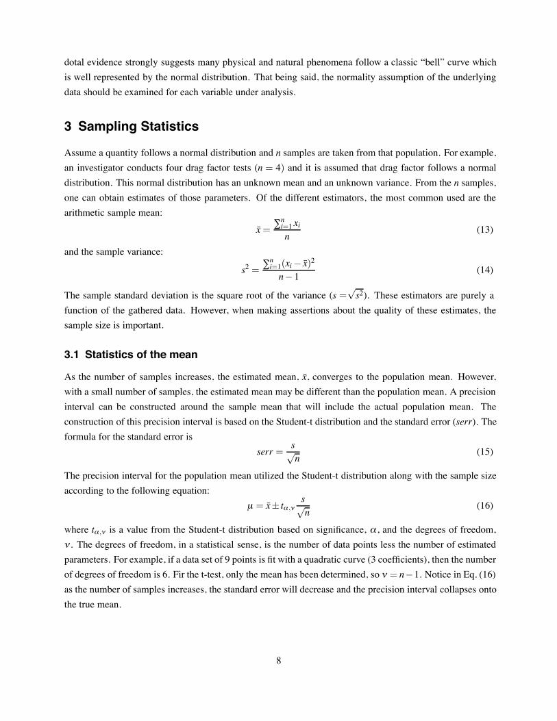
Figure 3: Examples of the Student-t distribution. The dashed line has 2 degrees of freedom, the solid linehas 5 d.o.f. and the dotted line is the standard normal.

The density function of the Student-t distribution is given by the following formula:

f (t) =(('+1

2 )(( k2 )[$' ]1/2[ t2' +1]('+1)/2

(17)

where ((x) is the generalized factorial or the Gamma function.Reconsider the example of the four drag factor tests. The sample mean was 0.744 with 4 degrees of

freedom. The sample standard deviation was 0.0181. Therefore, the standard error is calculated as

serr =s&n

=0.0181&

4= 0.00907.

If a 95% precision interval is desired, then the mean could change according to Eq. (17). The t value can bedetermined using a computer or a table, such as the one found in Refs. [13, 19, 20], to be t = 2.776. Usingthis information, the 95% precision interval for the mean of the population of specific drag factors is

µ = 0.744±2.776(0.00907)

which gives a lower bound for the mean of 0.719 and an upper bound for the mean as 0.769. Keep in mindthese are the bounds on the mean of the overall distribution of observed drag factors. The actual drag factora crash event may be outside this range.

3.2 Precision Interval of the Sample Variance

Following the argument for the sample mean, the sample variance can also change with subsequent observa-tions of a sample. Assuming the underlying population is normally distributed, the !2 (chi squared) statisticis used to define the precision interval for the population variance. Since the !2 distribution (shown in Fig.

9

0.05

0.10

0.15

0 1 2 3 4 5 6 7 8 9 10 11 12 13 14 15 16 17 18x

f (x)

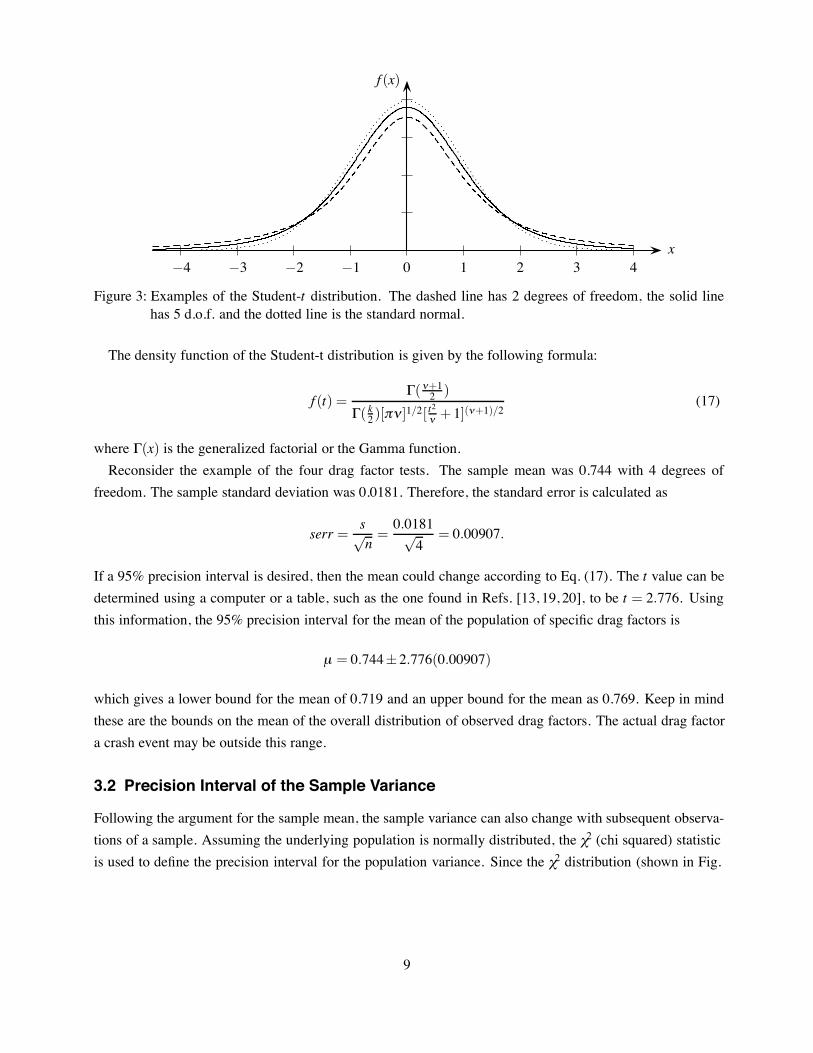
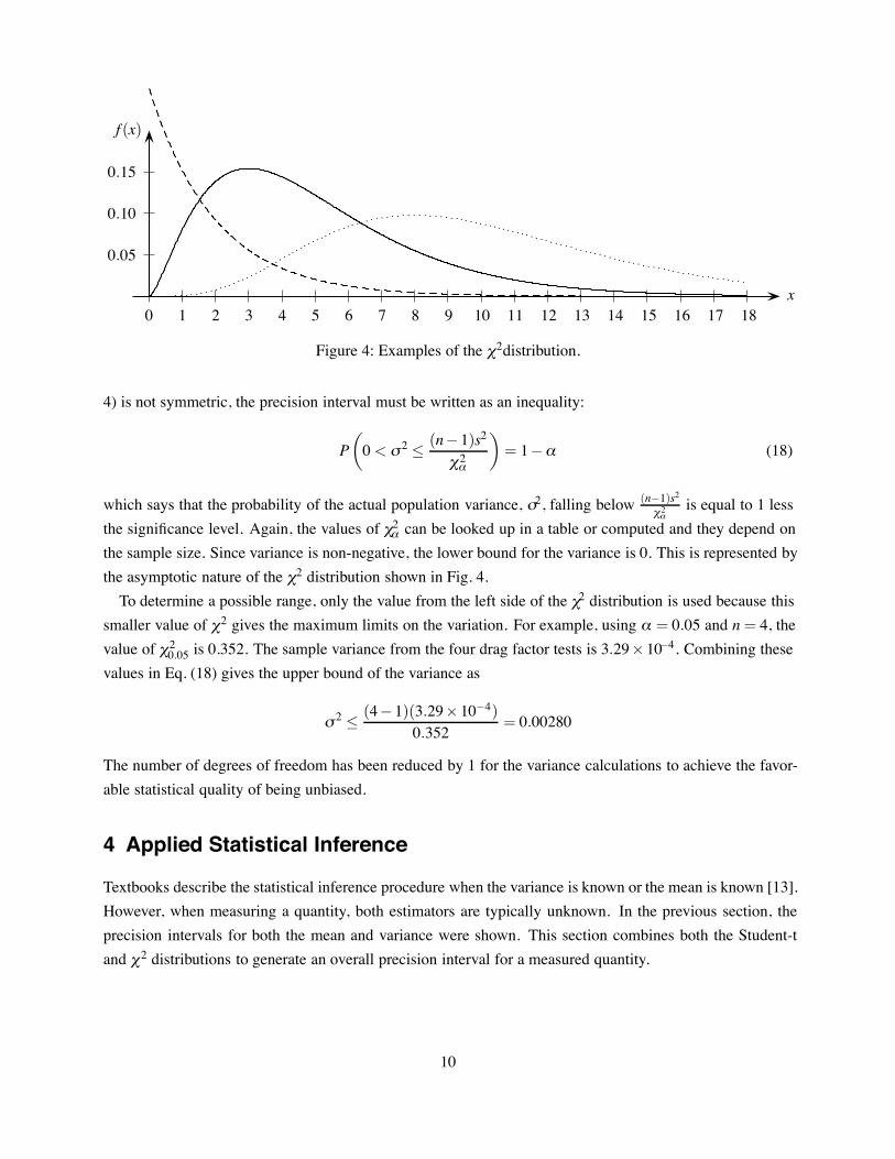
Figure 4: Examples of the !2distribution.

4) is not symmetric, the precision interval must be written as an inequality:

P'0< #2 " (n%1)s2

!2&

(= 1%& (18)

which says that the probability of the actual population variance, #2, falling below (n%1)s2!2&

is equal to 1 lessthe significance level. Again, the values of !2& can be looked up in a table or computed and they depend onthe sample size. Since variance is non-negative, the lower bound for the variance is 0. This is represented bythe asymptotic nature of the !2 distribution shown in Fig. 4.To determine a possible range, only the value from the left side of the !2 distribution is used because this

smaller value of !2 gives the maximum limits on the variation. For example, using & = 0.05 and n= 4, thevalue of !20.05 is 0.352. The sample variance from the four drag factor tests is 3.29'10%4. Combining thesevalues in Eq. (18) gives the upper bound of the variance as

# 2 " (4%1)(3.29'10%4)0.352

= 0.00280

The number of degrees of freedom has been reduced by 1 for the variance calculations to achieve the favor-able statistical quality of being unbiased.

4 Applied Statistical Inference

Textbooks describe the statistical inference procedure when the variance is known or the mean is known [13].However, when measuring a quantity, both estimators are typically unknown. In the previous section, theprecision intervals for both the mean and variance were shown. This section combines both the Student-tand !2 distributions to generate an overall precision interval for a measured quantity.

10

4.1 The Most Likely Estimate

The sample mean and sample standard deviation are the most likely values for the true population meanand standard deviation. Using only the most likely estimate (rather than a range of probable estimates), aprecision interval can be constructed based on the normal distribution.

x= x̄± z&s (19)

where z is the standard normal variate and & is the significance level (two-tailed). For the drag factor examplefrom Section 1.1 the values of f are computed as

f = 0.744±1.96(0.0181) = 0.744±0.0355 (95%)

This approach, while recognizing the inherent variability of the underlying measurement, x, fails to accountfor the variation of the estimates for the mean and standard deviation.

4.2 Variation of the Mean

Accounting for some error in the mean using the Student-t distribution and the standard error gives a largerrange than previously reported. When accounting for variation of the mean an using the most likely estimatefor the standard deviation, use the following formula to determine a range:

x= x̄± [(t' ,&)s&n

+ z&s] (20)

The example drag factors have 3 degrees of freedom so at the 95% significance level, t3,95 = 3.182. Asbefore, z95 = 1.96. Therefore, the range of drag factor data are:

f = 0.744± [3.182(0.0181)/&4+1.96(0.0181)] = 0.744±0.0643

Notice this interval is expanded from only using the normal distribution and the most likely estimates.

4.3 Variation of the Standard Deviation

The !2 distribution represents the variation of the variance according to Eq. (18). If the same logic is usedas in the last section, then a range can be determined as:

x= x̄± z&

)(n%1)s2!2n%1

(21)

11

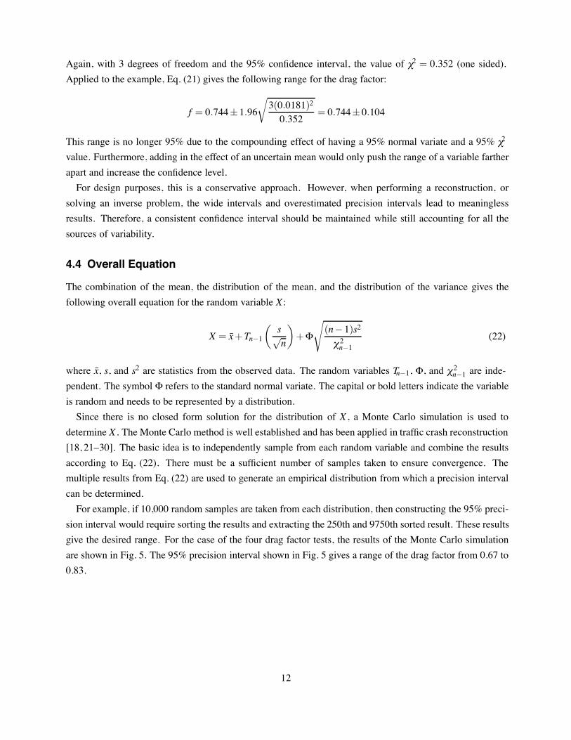
Again, with 3 degrees of freedom and the 95% confidence interval, the value of !2 = 0.352 (one sided).Applied to the example, Eq. (21) gives the following range for the drag factor:

f = 0.744±1.96*3(0.0181)20.352

= 0.744±0.104

This range is no longer 95% due to the compounding effect of having a 95% normal variate and a 95% !2

value. Furthermore, adding in the effect of an uncertain mean would only push the range of a variable fartherapart and increase the confidence level.For design purposes, this is a conservative approach. However, when performing a reconstruction, or

solving an inverse problem, the wide intervals and overestimated precision intervals lead to meaninglessresults. Therefore, a consistent confidence interval should be maintained while still accounting for all thesources of variability.

4.4 Overall Equation

The combination of the mean, the distribution of the mean, and the distribution of the variance gives thefollowing overall equation for the random variable X :

X = x̄+Tn%1'

s&n

(+)

)(n%1)s2!2n%1

(22)

where x̄, s, and s2 are statistics from the observed data. The random variables Tn%1, ), and !2n%1 are inde-pendent. The symbol ) refers to the standard normal variate. The capital or bold letters indicate the variableis random and needs to be represented by a distribution.Since there is no closed form solution for the distribution of X , a Monte Carlo simulation is used to

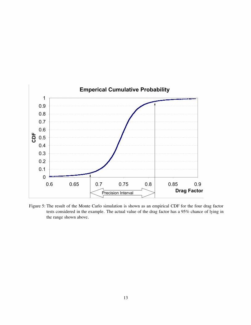
determine X . The Monte Carlo method is well established and has been applied in traffic crash reconstruction[18, 21–30]. The basic idea is to independently sample from each random variable and combine the resultsaccording to Eq. (22). There must be a sufficient number of samples taken to ensure convergence. Themultiple results from Eq. (22) are used to generate an empirical distribution from which a precision intervalcan be determined.For example, if 10,000 random samples are taken from each distribution, then constructing the 95% preci-

sion interval would require sorting the results and extracting the 250th and 9750th sorted result. These resultsgive the desired range. For the case of the four drag factor tests, the results of the Monte Carlo simulationare shown in Fig. 5. The 95% precision interval shown in Fig. 5 gives a range of the drag factor from 0.67 to0.83.

12

Emperical Cumulative Probability

00.10.20.30.40.50.60.70.80.9

1

0.6 0.65 0.7 0.75 0.8 0.85 0.9Drag Factor

CD

F

Precision Interval

Figure 5: The result of the Monte Carlo simulation is shown as an empirical CDF for the four drag factortests considered in the example. The actual value of the drag factor has a 95% chance of lying inthe range shown above.

13

2

3

4

5

6

7

8

0 5 10 15 20 25 30Number of Samples, n

Random

Variable,x

95% precisioninterval of thepopulation

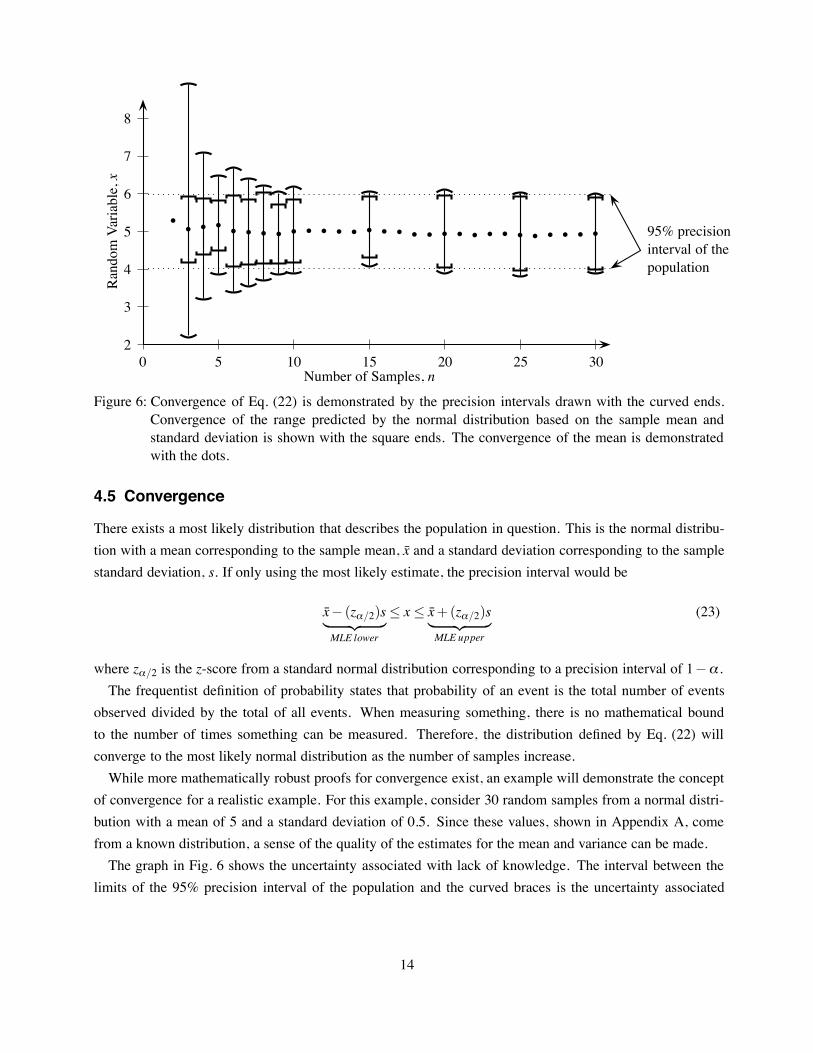
Figure 6: Convergence of Eq. (22) is demonstrated by the precision intervals drawn with the curved ends.Convergence of the range predicted by the normal distribution based on the sample mean andstandard deviation is shown with the square ends. The convergence of the mean is demonstratedwith the dots.

4.5 Convergence

There exists a most likely distribution that describes the population in question. This is the normal distribu-tion with a mean corresponding to the sample mean, x̄ and a standard deviation corresponding to the samplestandard deviation, s. If only using the most likely estimate, the precision interval would be

x̄% (z&/2)s+ ,- .MLE lower

" x" x̄+(z&/2)s+ ,- .MLE upper

(23)

where z&/2 is the z-score from a standard normal distribution corresponding to a precision interval of 1%& .The frequentist definition of probability states that probability of an event is the total number of events

observed divided by the total of all events. When measuring something, there is no mathematical boundto the number of times something can be measured. Therefore, the distribution defined by Eq. (22) willconverge to the most likely normal distribution as the number of samples increase.While more mathematically robust proofs for convergence exist, an example will demonstrate the concept

of convergence for a realistic example. For this example, consider 30 random samples from a normal distri-bution with a mean of 5 and a standard deviation of 0.5. Since these values, shown in Appendix A, comefrom a known distribution, a sense of the quality of the estimates for the mean and variance can be made.The graph in Fig. 6 shows the uncertainty associated with lack of knowledge. The interval between the

limits of the 95% precision interval of the population and the curved braces is the uncertainty associated

14

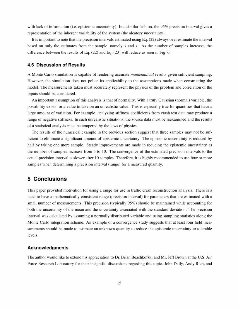
with lack of information (i.e. epistemic uncertainty). In a similar fashion, the 95% precision interval gives arepresentation of the inherent variability of the system (the aleatory uncertainty).It is important to note that the precision intervals estimated using Eq. (22) always over estimate the interval

based on only the estimates from the sample, namely x̄ and s. As the number of samples increase, thedifference between the results of Eq. (22) and Eq. (23) will reduce as seen in Fig. 6.

4.6 Discussion of Results

A Monte Carlo simulation is capable of rendering accurate mathematical results given sufficient sampling.However, the simulation does not police its applicability to the assumptions made when constructing themodel. The measurements taken must accurately represent the physics of the problem and correlation of theinputs should be considered.An important assumption of this analysis is that of normality. With a truly Gaussian (normal) variable, the

possibility exists for a value to take on an unrealistic value. This is especially true for quantities that have alarge amount of variation. For example, analyzing stiffness coefficients from crash test data may produce arange of negative stiffness. In such unrealistic situations, the source data must be reexamined and the resultsof a statistical analysis must be tempered by the laws of physics.The results of the numerical example in the previous section suggest that three samples may not be suf-

ficient to eliminate a significant amount of epistemic uncertainty. The epistemic uncertainty is reduced byhalf by taking one more sample. Steady improvements are made in reducing the epistemic uncertainty asthe number of samples increase from 5 to 10. The convergence of the estimated precision intervals to theactual precision interval is slower after 10 samples. Therefore, it is highly recommended to use four or moresamples when determining a precision interval (range) for a measured quantity.

5 Conclusions

This paper provided motivation for using a range for use in traffic crash reconstruction analysis. There is aneed to have a mathematically consistent range (precision interval) for parameters that are estimated with asmall number of measurements. This precision (typically 95%) should be maintained while accounting forboth the uncertainty of the mean and the uncertainty associated with the standard deviation. The precisioninterval was calculated by assuming a normally distributed variable and using sampling statistics along theMonte Carlo integration scheme. An example of a convergence study suggests that at least four field mea-surements should be made to estimate an unknown quantity to reduce the epistemic uncertainty to tolerablelevels.

Acknowledgments

The author would like to extend his appreciation to Dr. Brian Beachkofski and Mr. Jeff Brown at the U.S. AirForce Research Laboratory for their insightful discussions regarding this topic. John Daily, Andy Rich, and

15

Bill Messerschmidt also provided insightful suggestions. Finally, the author would like to acknowledge theIllinois Association of Technical Accident Investigators (IATAI) for requesting this topic be explored.

Notation

The following symbols are used in this paper:Symbol Meaning

x̄ = sample meanµ = population means = sample standard deviation# = population standard deviation

f (·) = Functional form for a probability density functionf = drag factor

F(·) = functional form for a cumulative distribution functionx = variable, measurementX = random variablen = number of samples' = degrees of freedom

serr = standard deviation of the mean& = significance levelz = z-score for a standard normal distributionT' = student-t distribution with ' degrees of freedom) = the standard normal variate!2 = the chi-squared distribution

References

[1] W. Bartlett et al., “Evaluating the uncertianty in various measurement tasks common to accident recon-struction,” in Accident Reconstruction SP-1666, ser. SP. Society of Automotive Engineers, Warrendale,PA, March 2002, no. 2002-01-0546, pp. 57–70.

[2] W. Bartlett and A. Fonda, “Evaluating uncertainty in accident reconstruction with finite differences,”SAE Technical Paper Series, vol. SP-1773, no. 2003-01-0489, Jan 2003.

[3] R. Brach, “Uncertainty in accident reconstruction calculations,” SAE Technical Paper Series, vol. SP-1030, no. 940722, 1994.

[4] A. Fonda, “The effects of measurement uncertainty on the reconstruction of various vehicular colli-sions,” SAE Technical Paper Series, vol. SP-1873, no. 2004-01-1220, Jan 2004.

16

[5] F. Navin, “The accuracy and precision of speed estimates from accident reconstruction data,” in SpecialProblems, IPTM. Jacksonville, FL: UNF, May 2000.

[6] R. W. Rivers, Advanced Traffic Accident Investigation. Jacksonville: Institute of Police Technologyand Management, 1997.

[7] R. H. Dieck, Measurement Uncertainty: Methods and Applications, 3rd ed. Research Triangle Park,NC: The Intrumentation, Systems and Automation Society, 2002.

[8] J. G. Daily et al., Fundamentals of Traffic Crash Reconstruction. Jacksonville, Fl: Institute of PoliceTechnology and Management, University of North Florida, 2006.

[9] B. Roberson and G. A. Vignaux, Interpreting Evidence: Evaluating Foresic Science in the Courtroom.Chichester: John Wiley & Sons, 1995.

[10] C. C. O.Marks, “Accident analysis uncertianty in the forensic context,” 2002, personal Communication.

[11] C. G. G. Aitken and F. Taroni, Statistics and the Evaluation of Evidence for Forensic Scientists. Chich-ester: John Wiley & Sons, 2004.

[12] G. Davis, “Bayesian reconstruction of traffic accidents,” Law, Probability and Risk, vol. 2, no. 2, pp.69–89, Jan 2003.

[13] B. M. Ayyub and R. H. McCuen, Probability, Statistics, and Reliability for Engineers. Boca Raton:CRC Press LLC, 1997.

[14] W. L. Oberkampf et al., “Mathematical representation of uncertainty,” American Institute of Aeronau-tics and Astronautics (AIAA), no. 1645, pp. 1–22, 2001.

[15] E. Kreyszig, Introductory Mathematical Statistics. New York: John Wiley, 1970.

[16] E. W. Weisstein, “Monte carlo method,” May 2006, from MathWorld–A Wolfram Web Resource.http://mathworld.wolfram.com/MonteCarloMethod.html.

[17] B. Efron, The Jackknife, the Bootstrap and other Resampling Plans. Philadelphia: Society for Indus-trial and Applied Mathematics, 1982.

[18] J. Ball, D. Danaher, and R. Ziernicki, “Considerations for applying and interpreting monte carlo simu-lation analyses in accident . . . ,” SAE Technical Paper Series, no. 2007-01-0741, Jan 2007.

[19] D. J. Sheskin, Handbook of Parapmetric and Nonparametric Statistical Procedures. Boca Raton:Chapman & Hall / CRC, 2000.

[20] D. C. Montgomery, Design and Analysis of Experiments, 5th ed. New York: John Wiley and Sons,2004, a complete discussion of designing, conducting, and analyzing experiments.

17

[21] G. Kost and S. M. Werner, “Use of Monte Carlo simulation techniques in accident reconstruction,” SAETechnical Paper Series, no. 940719, 1994.

[22] D. P. Wood and S. O’Riordain, “Monte carlo simulation methods applied to accident reconstruction andavoidance analysis,” SAE Technical Paper Series, no. 940720, 1994.

[23] W. Bartlett, “Conducting monte Carlo analysis with spreadsheet programs,” SAE Technical Paper Se-ries, no. 2003-01-0487, 2003.

[24] S. Kimbrough, “Determining the relative likelihoods of competing scenarios of events leading to anaccident,” SAE Technical Paper Series, no. 2004-01-1222, p. 14, Dec 2004.

[25] Z. Lozia and M. Guzek, “Uncertainty study of road accident reconstruction-computational methods,”SAE Technical Paper Series, vol. SP-1930, no. 2005-01-1195, Jan 2005.

[26] A. Moser, H. Steffan, A. Spek, and W.Makkinga, “Application of the Monte Carlo methods for stabilityanalysis within the accident reconstruction software PC-CRASH,” SAE Technical Paper Series, 2003-01-0488.

[27] M. A. Piskie and T. Gioutsos, “Automibile crash modeling and theMonte Carlo method,” SAE TechnicalPaper Series, no. 920480, 1992.

[28] N. A. Rose, S. J. Fenton, and C. M. Hughes, “Integrating Monte Carlo simulation, momentum-basedimpact modeling, and restitution data to analyze crash severity,” SAE Technical Paper Series, 2001-01-0907.

[29] W. Wach and J. Unarski, “Determination of vehicle velocities and collision location by means of montecarlo simulation method,” SAE Technical Paper Series, no. 2006-01-0907, 2006.

[30] ——, “Uncertainty of calculation results in vehicle collision analysis,” Forensic Science International,vol. 167, no. 2-3, pp. 181–188, Apr 2007.

A Random Samples

The following is a list of random samples from a normal distribution with a mean of 5 and a standarddeviation of 0.5. These values were used in the analysis to generate Fig. 6. The values used are 5.062, 5.523,4.607, 5.312, 5.345, 4.237, 4.819, 4.735, 4.815, 5.622, 5.187, 4.940, 4.800, 4.911, 5.675, 4.497, 4.788, 3.770,4.866, 5.342, 4.849, 4.292, 5.542, 5.127, 4.006, 4.318, 5.779, 5.070, 5.003, and 5.580. The 95% precisioninterval for the underlying population is

4.020 < x< 5.980

as shown by the dotted lines of Fig. 6.

18