Uncertainty quantification in analytical and finite element beam modelsusing experimental data

P. Langer, K. Sepahvand and S. MarburgInstitute of Mechanics, Universitat der Bundeswehr, Munich, Germany

Patrick.Langer@unibw.de

ABSTRACT: This study describes the quality of model formation for free vibration of beam structures underuncertainty. The key issues are that all analytical and numerical finite element (FE) models contain uncertaintiesdue to the tolerances in topological parameters, assumptions made, material parameters, boundary conditions. Twowell–known Euler–Bernoulli and Timoshenko beam theories have been compared. At FE level, various elementsavailable for modeling of beam structures in ABAQUS are compared and evaluated. Experimental modal analysishave been performed on beam specimens to validate the results from analytical and FE models due to parameteruncertainties. It is shown which element types are required to allow minimal deviation from the experimental resultsconsidering uncertainties.

Keywords: Uncertainty quantification, FE modeling, beam structures, experimental modal analysis

1 Introduction

By definition, a model is an abstraction of reality in which manyassumptions are made. It is not possible to evaluate correct resultswithout knowing the underlying assumptions [1, 2]. For this reasonit is important to find exactly the right model that is the most suitablefor the conceptual formulation. In the formation of the mathematicalmodels the minimum description length principle (MDL) proposedby Rissanen [3] is one useful approach to finding the shortest de-scription of the data and the model itself. Ross Quinlan and Rivesprovide a good description of MDL principle in [4]. The method,however, does not include the estimation of errors in the results.Model building and simulation are becoming increasingly impor-tant in engineering. In simulation phase, the Finite Element Method(FEM) is manly used to construct a numerical model. Within thepast decade increasing in computer capability, FEM has becomehighly important in model formation for engineers. Additionally,in industry, FEM has crucial importance for reducing the numberof experimental examinations. The major issue is that every FEMmodel possess some degree of uncertainty due to topological andmaterial parameters, initial and boundary conditions, forcing term,etc. The results from FEM models are trustable if they are validatedwith experimental or results from available analytical models. Whencomparing the models, however, uncertainties must be taken into ac-count. General recommendations regarding model uncertainties aregiven in [5] that are important for model formation and in the devel-opment process. A powerful tool in numerical simulation of engi-neering problems involve uncertainty is the stochastic finite elementmethod (SFEM), which is an extension of deterministic FEM in ran-dom framework [6]. The application of the method on various prac-tical engineering problems including uncertainty has been studied inmany works, cf. [7–12]This paper present a comparison of numerical, analytical models andthe experimental results for beam structures involving material and

parameter uncertainties. The results have been studied for variousquadratic tetrahedral and hexahedral elements types with differentnumber of elements to realize the model uncertainties. The one–dimensional solution obtained by Euler–Bernoulli and Timoshenkowas used for the analyses in this study. The physical model for exper-imental results depends on the precision of the measuring equipmentand the apparatus used to perform an experiment. The considereduncertainties include material and shape, while model uncertaintiesinclude boundary conditions, model assumptions, model depth andlevel of detail. The model depth, is, by definition, the formation ofelements, and the level of detail is the number of elements. The in-vestigation includes a study of the model depth and the level of detailin which the FE model is verified for the analytical solution is firstdescribed, this is followed by verification for an overkill calculation.The physical, numerical and analytical models will be compared us-ing the best regular mesh determined. A recommendation is givensince a virtual image for exactly one simple real shape can be made.Abaqus/CAE was used as a pre- and postprocessor for this task. Inthe experimental modal analysis, the free–free beam specimens werecontact free excited by a periodic chirp signal by means of loud-speakers. The resonance frequencies of the first 3 bending modeswere measured with a Laser–Doppler–Vibrometer.The remainder of the paper is organized as follows. Section 2 reviewsthe investigated FEM, analytical and experimental models. The nu-merical simulations of the method illustrate in section 3. Section 4discusses the conclusions.

2 Model description

In this section, we discuss the details of FEM, analytical and experi-mental models considered in the investigation.

1

Proceedings of the 9th International Conference on Structural Dynamics, EURODYN 2014Porto, Portugal, 30 June - 2 July 2014

A. Cunha, E. Caetano, P. Ribeiro, G. Müller (eds.)ISSN: 2311-9020; ISBN: 978-972-752-165-4

2753

2.1 FEM models

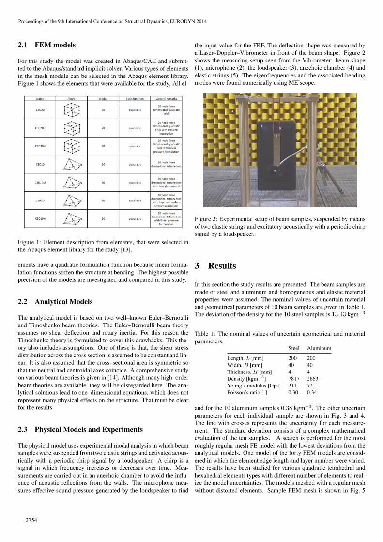
For this study the model was created in Abaqus/CAE and submit-ted to the Abaqus/standard implicit solver. Various types of elementsin the mesh module can be selected in the Abaqus element library.Figure 1 shows the elements that were available for the study. All el-

Figure 1: Element description from elements, that were selected inthe Abaqus element library for the study [13].

ements have a quadratic formulation function because linear formu-lation functions stiffen the structure at bending. The highest possibleprecision of the models are investigated and compared in this study.

2.2 Analytical Models

The analytical model is based on two well–known Euler–Bernoulliand Timoshenko beam theories. The Euler–Bernoulli beam theoryassumes no shear deflection and rotary inertia. For this reason theTimoshenko theory is formulated to cover this drawbacks. This the-ory also includes assumptions. One of these is that, the shear stressdistribution across the cross section is assumed to be constant and lin-ear. It is also assumed that the cross–sectional area is symmetric sothat the neutral and centroidal axes coincide. A comprehensive studyon various beam theories is given in [14]. Although many high–orderbeam theories are available, they will be disregarded here. The ana-lytical solutions lead to one–dimensional equations, which does notrepresent many physical effects on the structure. That must be clearfor the results.

2.3 Physical Models and Experiments

The physical model uses experimental modal analysis in which beamsamples were suspended from two elastic strings and activated acous-tically with a periodic chirp signal by a loudspeaker. A chirp is asignal in which frequency increases or decreases over time. Mea-surements are carried out in an anechoic chamber to avoid the influ-ence of acoustic reflections from the walls. The microphone mea-sures effective sound pressure generated by the loudspeaker to find

the input value for the FRF. The deflection shape was measured bya Laser–Doppler–Vibrometer in front of the beam shape. Figure 2shows the measuring setup seen from the Vibrometer: beam shape(1), microphone (2), the loudspeaker (3), anechoic chamber (4) andelastic strings (5). The eigenfrequencies and the associated bendingmodes were found numerically using ME’scope.

1

2

3

4

5

Figure 2: Experimental setup of beam samples, suspended by meansof two elastic strings and excitatory acoustically with a periodic chirpsignal by a loudspeaker.

3 Results

In this section the study results are presented. The beam samples aremade of steel and aluminum and homogeneous and elastic materialproperties were assumed. The nominal values of uncertain materialand geometrical parameters of 10 beam samples are given in Table 1.The deviation of the density for the 10 steel samples is 13.43 kgm−3

Table 1: The nominal values of uncertain geometrical and materialparameters.

Steel Aluminum

Length, L [mm] 200 200Width, B [mm] 40 40Thickness, H [mm] 4 4Density [kgm−3] 7817 2663Young’s modulus [Gpa] 211 72Poisson’s ratio [-] 0.30 0.34

and for the 10 aluminum samples 0.38 kgm−3. The other uncertainparameters for each individual sample are shown in Fig. 3 and 4.The line with crosses represents the uncertainty for each measure-ment. The standard deviation consists of a complex mathematicalevaluation of the ten samples. A search is performed for the mostroughly regular mesh FE model with the lowest deviations from theanalytical models. One model of the forty FEM models are consid-ered in which the element edge length and layer number were varied.The results have been studied for various quadratic tetrahedral andhexahedral elements types with different number of elements to real-ize the model uncertainties. The models meshed with a regular meshwithout distorted elements. Sample FEM mesh is shown in Fig. 5

2

Proceedings of the 9th International Conference on Structural Dynamics, EURODYN 2014

2754

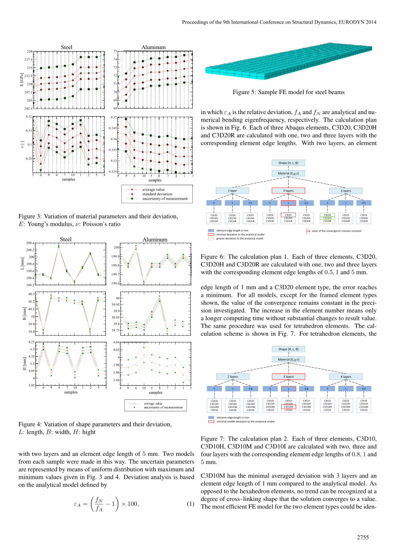
Figure 3: Variation of material parameters and their deviation,E: Young’s modulus, ν: Poisson’s ratio

Figure 4: Variation of shape parameters and their deviation,L: length, B: width, H: hight

with two layers and an element edge length of 5 mm. Two modelsfrom each sample were made in this way. The uncertain parametersare represented by means of uniform distribution with maximum andminimum values given in Fig. 3 and 4. Deviation analysis is basedon the analytical model defined by

εA =

(fNfA

− 1

)× 100, (1)

Figure 5: Sample FE model for steel beams

in which εA is the relative deviation, fA and fN are analytical and nu-merical bending eigenfrequency, respectively. The calculation planis shown in Fig. 6. Each of three Abaqus elements, C3D20, C3D20Hand C3D20R are calculated with one, two and three layers with thecorresponding element edge lengths. With two layers, an element

F

Shape [H, L, B]

Material [E, , ]

1 layer 2 layers 3 layers

5 1 0.5 5 1 0.5 5 1 0.5

C3D20 C3D20H C3D20R

C3D20 C3D20H C3D20R

C3D20 C3D20H C3D20R

C3D20 C3D20H C3D20R

C3D20 C3D20H C3D20R

C3D20 C3D20H C3D20R

C3D20 C3D20H C3D20R

C3D20 C3D20H C3D20R

C3D20 C3D20H C3D20R

minimal deviation to the analytical model value of the convergence remains constant

greater deviation to the analytical model

element edge length in mm

Figure 6: The calculation plan 1. Each of three elements, C3D20,C3D20H and C3D20R are calculated with one, two and three layerswith the corresponding element edge lengths of 0.5, 1 and 5 mm.

edge length of 1 mm and a C3D20 element type, the error reachesa minimum. For all models, except for the framed element typesshown, the value of the convergence remains constant in the preci-sion investigated. The increase in the element number means onlya longer computing time without substantial changes to result value.The same procedure was used for tetrahedron elements. The cal-culation scheme is shown in Fig. 7. For tetrahedron elements, the

F

Shape [H, L, B]

Material [E, , ]

2 layers 3 layers 4 layers

5 1 0.8 5 1 0.8 5 1 0.8

C3D10 C3D10H C3D10M C3D10I

C3D10 C3D10H C3D10M C3D10I

C3D10 C3D10H C3D10M C3D10I

C3D10 C3D10H C3D10M C3D10I

C3D10 C3D10H C3D10M C3D10I

C3D10 C3D10H C3D10M C3D10I

C3D10 C3D10H C3D10M C3D10I

C3D10 C3D10H C3D10M C3D10I

C3D10 C3D10H C3D10M C3D10I

minimal middle deviation to the analytical model element edge length in mm

Figure 7: The calculation plan 2. Each of three elements, C3D10,C3D10H, C3D10M and C3D10I are calculated with two, three andfour layers with the corresponding element edge lengths of 0.8, 1 and5 mm.

C3D10M has the minimal averaged deviation with 3 layers and anelement edge length of 1 mm compared to the analytical model. Asopposed to the hexahedron elements, no trend can be recognized at adegree of cross–linking shape that the solution converges to a value.The most efficient FE model for the two element types could be iden-

3

Proceedings of the 9th International Conference on Structural Dynamics, EURODYN 2014

2755

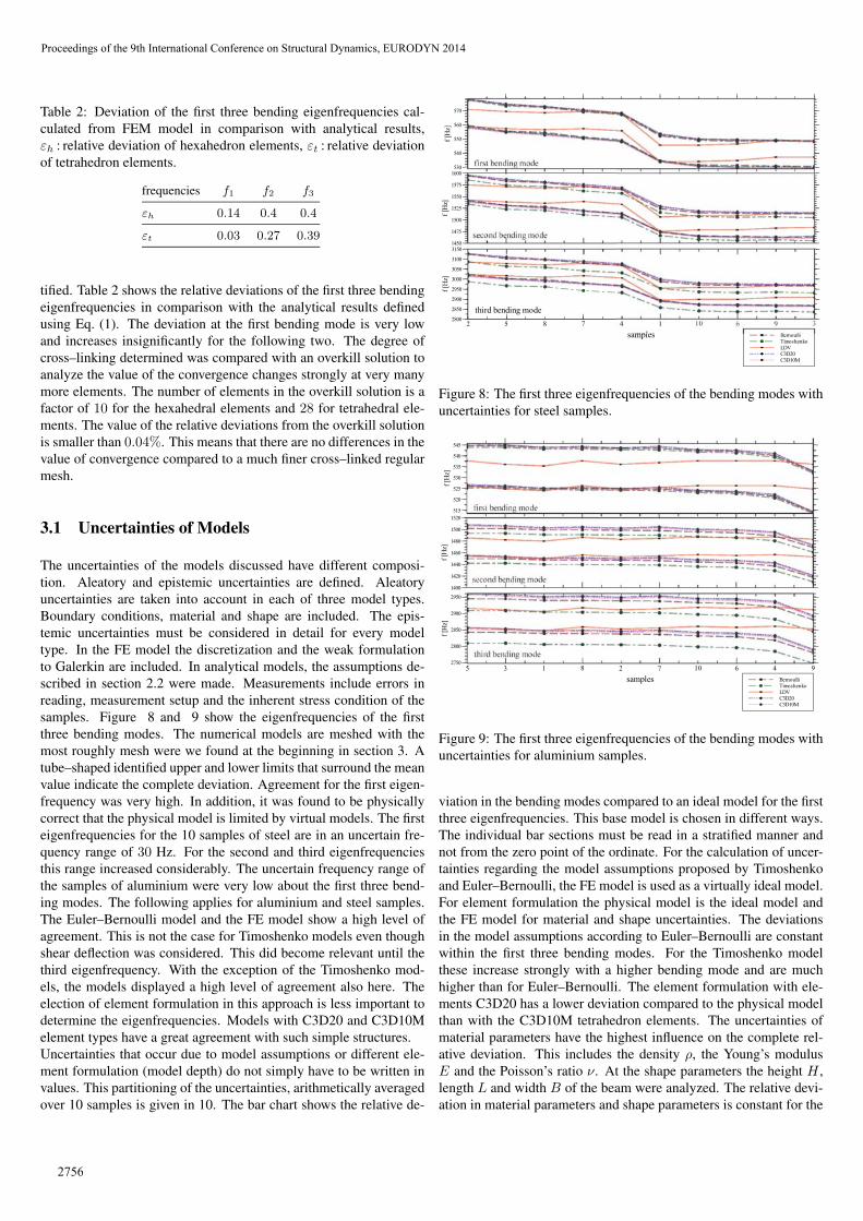
Table 2: Deviation of the first three bending eigenfrequencies cal-culated from FEM model in comparison with analytical results,εh : relative deviation of hexahedron elements, εt : relative deviationof tetrahedron elements.

frequencies f1 f2 f3

εh 0.14 0.4 0.4

εt 0.03 0.27 0.39

tified. Table 2 shows the relative deviations of the first three bendingeigenfrequencies in comparison with the analytical results definedusing Eq. (1). The deviation at the first bending mode is very lowand increases insignificantly for the following two. The degree ofcross–linking determined was compared with an overkill solution toanalyze the value of the convergence changes strongly at very manymore elements. The number of elements in the overkill solution is afactor of 10 for the hexahedral elements and 28 for tetrahedral ele-ments. The value of the relative deviations from the overkill solutionis smaller than 0.04%. This means that there are no differences in thevalue of convergence compared to a much finer cross–linked regularmesh.

3.1 Uncertainties of Models

The uncertainties of the models discussed have different composi-tion. Aleatory and epistemic uncertainties are defined. Aleatoryuncertainties are taken into account in each of three model types.Boundary conditions, material and shape are included. The epis-temic uncertainties must be considered in detail for every modeltype. In the FE model the discretization and the weak formulationto Galerkin are included. In analytical models, the assumptions de-scribed in section 2.2 were made. Measurements include errors inreading, measurement setup and the inherent stress condition of thesamples. Figure 8 and 9 show the eigenfrequencies of the firstthree bending modes. The numerical models are meshed with themost roughly mesh were we found at the beginning in section 3. Atube–shaped identified upper and lower limits that surround the meanvalue indicate the complete deviation. Agreement for the first eigen-frequency was very high. In addition, it was found to be physicallycorrect that the physical model is limited by virtual models. The firsteigenfrequencies for the 10 samples of steel are in an uncertain fre-quency range of 30 Hz. For the second and third eigenfrequenciesthis range increased considerably. The uncertain frequency range ofthe samples of aluminium were very low about the first three bend-ing modes. The following applies for aluminium and steel samples.The Euler–Bernoulli model and the FE model show a high level ofagreement. This is not the case for Timoshenko models even thoughshear deflection was considered. This did become relevant until thethird eigenfrequency. With the exception of the Timoshenko mod-els, the models displayed a high level of agreement also here. Theelection of element formulation in this approach is less important todetermine the eigenfrequencies. Models with C3D20 and C3D10Melement types have a great agreement with such simple structures.Uncertainties that occur due to model assumptions or different ele-ment formulation (model depth) do not simply have to be written invalues. This partitioning of the uncertainties, arithmetically averagedover 10 samples is given in 10. The bar chart shows the relative de-

Figure 8: The first three eigenfrequencies of the bending modes withuncertainties for steel samples.

Figure 9: The first three eigenfrequencies of the bending modes withuncertainties for aluminium samples.

viation in the bending modes compared to an ideal model for the firstthree eigenfrequencies. This base model is chosen in different ways.The individual bar sections must be read in a stratified manner andnot from the zero point of the ordinate. For the calculation of uncer-tainties regarding the model assumptions proposed by Timoshenkoand Euler–Bernoulli, the FE model is used as a virtually ideal model.For element formulation the physical model is the ideal model andthe FE model for material and shape uncertainties. The deviationsin the model assumptions according to Euler–Bernoulli are constantwithin the first three bending modes. For the Timoshenko modelthese increase strongly with a higher bending mode and are muchhigher than for Euler–Bernoulli. The element formulation with ele-ments C3D20 has a lower deviation compared to the physical modelthan with the C3D10M tetrahedron elements. The uncertainties ofmaterial parameters have the highest influence on the complete rel-ative deviation. This includes the density ρ, the Young’s modulusE and the Poisson’s ratio ν. At the shape parameters the height H ,length L and width B of the beam were analyzed. The relative devi-ation in material parameters and shape parameters is constant for the

4

Proceedings of the 9th International Conference on Structural Dynamics, EURODYN 2014

2756

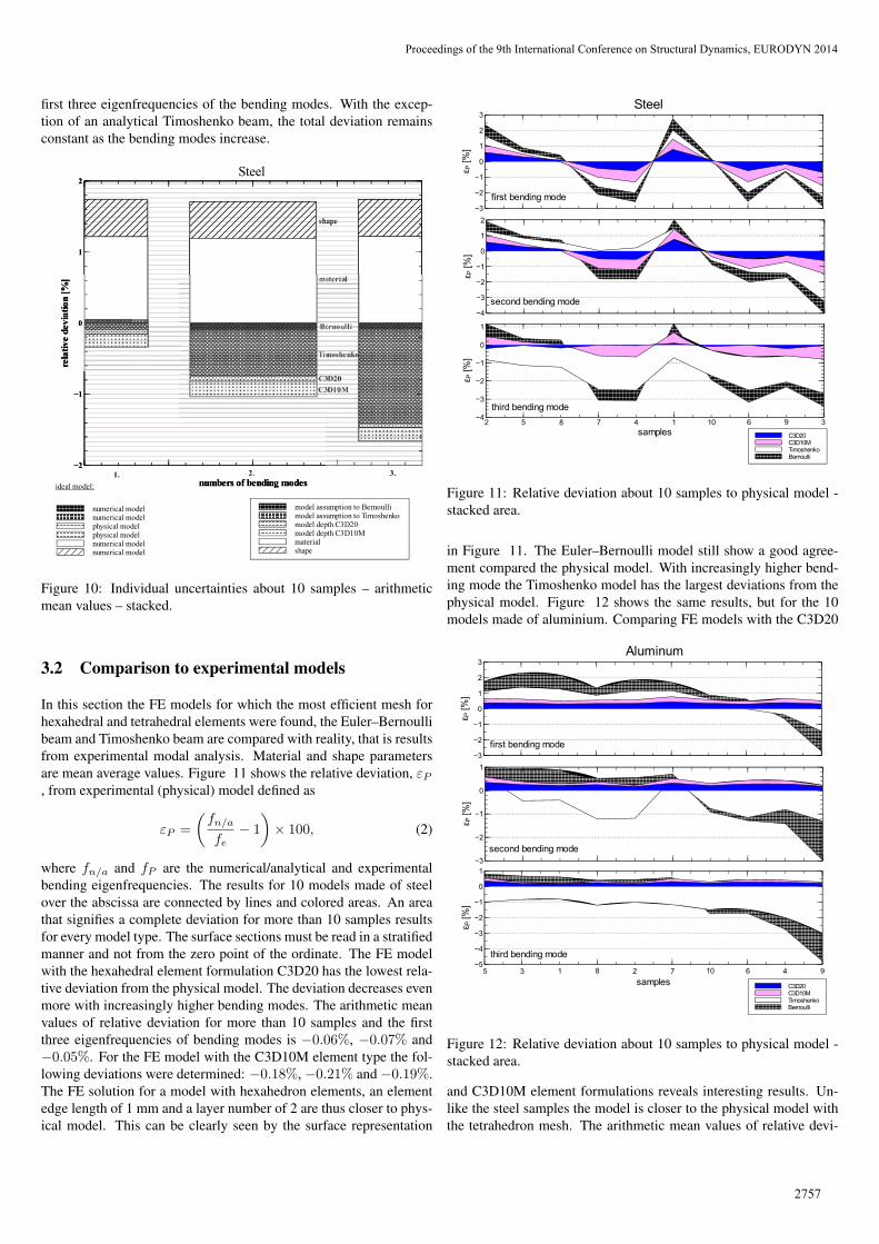
first three eigenfrequencies of the bending modes. With the excep-tion of an analytical Timoshenko beam, the total deviation remainsconstant as the bending modes increase.

Figure 10: Individual uncertainties about 10 samples – arithmeticmean values – stacked.

3.2 Comparison to experimental models

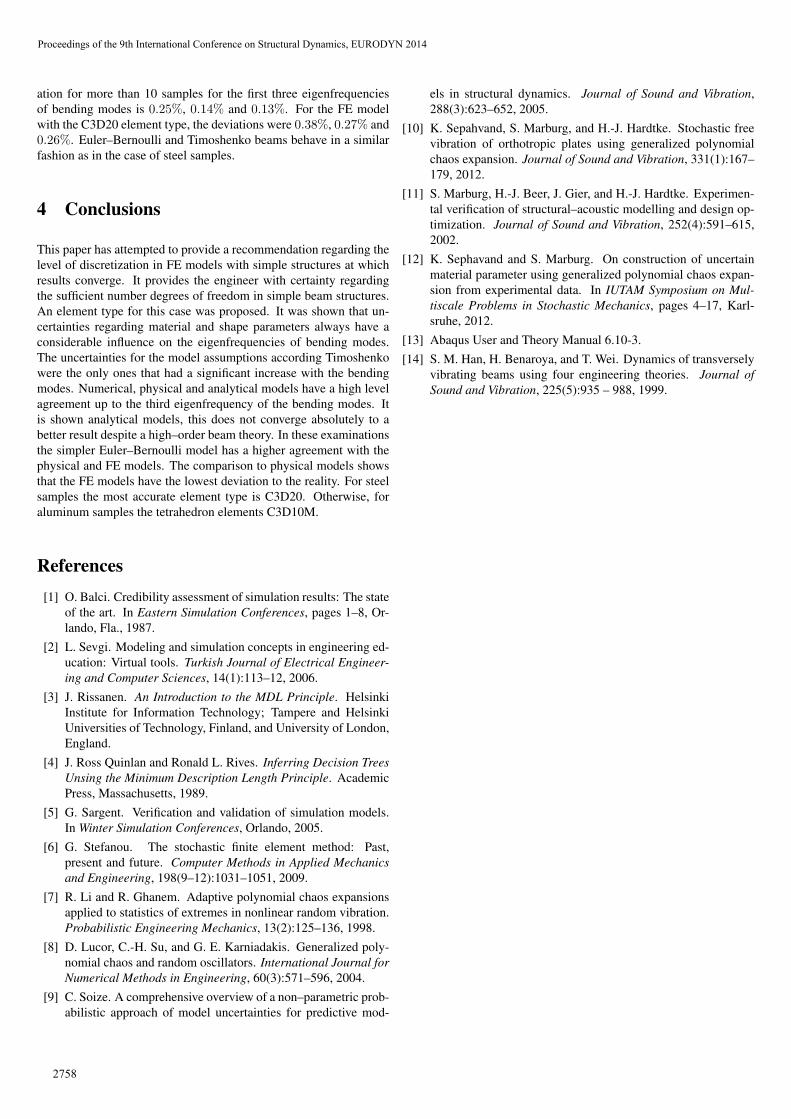
In this section the FE models for which the most efficient mesh forhexahedral and tetrahedral elements were found, the Euler–Bernoullibeam and Timoshenko beam are compared with reality, that is resultsfrom experimental modal analysis. Material and shape parametersare mean average values. Figure 11 shows the relative deviation, εP, from experimental (physical) model defined as

εP =

(fn/a

fe− 1

)× 100, (2)

where fn/a and fP are the numerical/analytical and experimentalbending eigenfrequencies. The results for 10 models made of steelover the abscissa are connected by lines and colored areas. An areathat signifies a complete deviation for more than 10 samples resultsfor every model type. The surface sections must be read in a stratifiedmanner and not from the zero point of the ordinate. The FE modelwith the hexahedral element formulation C3D20 has the lowest rela-tive deviation from the physical model. The deviation decreases evenmore with increasingly higher bending modes. The arithmetic meanvalues of relative deviation for more than 10 samples and the firstthree eigenfrequencies of bending modes is −0.06%, −0.07% and−0.05%. For the FE model with the C3D10M element type the fol-lowing deviations were determined: −0.18%, −0.21% and −0.19%.The FE solution for a model with hexahedron elements, an elementedge length of 1 mm and a layer number of 2 are thus closer to phys-ical model. This can be clearly seen by the surface representation

Figure 11: Relative deviation about 10 samples to physical model -stacked area.

in Figure 11. The Euler–Bernoulli model still show a good agree-ment compared the physical model. With increasingly higher bend-ing mode the Timoshenko model has the largest deviations from thephysical model. Figure 12 shows the same results, but for the 10models made of aluminium. Comparing FE models with the C3D20

Figure 12: Relative deviation about 10 samples to physical model -stacked area.

and C3D10M element formulations reveals interesting results. Un-like the steel samples the model is closer to the physical model withthe tetrahedron mesh. The arithmetic mean values of relative devi-

5

Proceedings of the 9th International Conference on Structural Dynamics, EURODYN 2014

2757

ation for more than 10 samples for the first three eigenfrequenciesof bending modes is 0.25%, 0.14% and 0.13%. For the FE modelwith the C3D20 element type, the deviations were 0.38%, 0.27% and0.26%. Euler–Bernoulli and Timoshenko beams behave in a similarfashion as in the case of steel samples.

4 Conclusions

This paper has attempted to provide a recommendation regarding thelevel of discretization in FE models with simple structures at whichresults converge. It provides the engineer with certainty regardingthe sufficient number degrees of freedom in simple beam structures.An element type for this case was proposed. It was shown that un-certainties regarding material and shape parameters always have aconsiderable influence on the eigenfrequencies of bending modes.The uncertainties for the model assumptions according Timoshenkowere the only ones that had a significant increase with the bendingmodes. Numerical, physical and analytical models have a high levelagreement up to the third eigenfrequency of the bending modes. Itis shown analytical models, this does not converge absolutely to abetter result despite a high–order beam theory. In these examinationsthe simpler Euler–Bernoulli model has a higher agreement with thephysical and FE models. The comparison to physical models showsthat the FE models have the lowest deviation to the reality. For steelsamples the most accurate element type is C3D20. Otherwise, foraluminum samples the tetrahedron elements C3D10M.

References[1] O. Balci. Credibility assessment of simulation results: The state

of the art. In Eastern Simulation Conferences, pages 1–8, Or-lando, Fla., 1987.

[2] L. Sevgi. Modeling and simulation concepts in engineering ed-ucation: Virtual tools. Turkish Journal of Electrical Engineer-ing and Computer Sciences, 14(1):113–12, 2006.

[3] J. Rissanen. An Introduction to the MDL Principle. HelsinkiInstitute for Information Technology; Tampere and HelsinkiUniversities of Technology, Finland, and University of London,England.

[4] J. Ross Quinlan and Ronald L. Rives. Inferring Decision TreesUnsing the Minimum Description Length Principle. AcademicPress, Massachusetts, 1989.

[5] G. Sargent. Verification and validation of simulation models.In Winter Simulation Conferences, Orlando, 2005.

[6] G. Stefanou. The stochastic finite element method: Past,present and future. Computer Methods in Applied Mechanicsand Engineering, 198(9–12):1031–1051, 2009.

[7] R. Li and R. Ghanem. Adaptive polynomial chaos expansionsapplied to statistics of extremes in nonlinear random vibration.Probabilistic Engineering Mechanics, 13(2):125–136, 1998.

[8] D. Lucor, C.-H. Su, and G. E. Karniadakis. Generalized poly-nomial chaos and random oscillators. International Journal forNumerical Methods in Engineering, 60(3):571–596, 2004.

[9] C. Soize. A comprehensive overview of a non–parametric prob-abilistic approach of model uncertainties for predictive mod-

els in structural dynamics. Journal of Sound and Vibration,288(3):623–652, 2005.

[10] K. Sepahvand, S. Marburg, and H.-J. Hardtke. Stochastic freevibration of orthotropic plates using generalized polynomialchaos expansion. Journal of Sound and Vibration, 331(1):167–179, 2012.

[11] S. Marburg, H.-J. Beer, J. Gier, and H.-J. Hardtke. Experimen-tal verification of structural–acoustic modelling and design op-timization. Journal of Sound and Vibration, 252(4):591–615,2002.

[12] K. Sephavand and S. Marburg. On construction of uncertainmaterial parameter using generalized polynomial chaos expan-sion from experimental data. In IUTAM Symposium on Mul-tiscale Problems in Stochastic Mechanics, pages 4–17, Karl-sruhe, 2012.

[13] Abaqus User and Theory Manual 6.10-3.[14] S. M. Han, H. Benaroya, and T. Wei. Dynamics of transversely

vibrating beams using four engineering theories. Journal ofSound and Vibration, 225(5):935 – 988, 1999.

6

Proceedings of the 9th International Conference on Structural Dynamics, EURODYN 2014

2758