Uncertainty, Reputation and Analyst Coverage

Marco Navone∗

UTS Business School, University of Technology Sydney, Sydney, NSW 2007, AUSTRALIA

Fernando Zapatero

USC Marshall School of Business, University of Southern California, Los Angeles, CA 90089, USA

ABSTRACT

In this paper we investigate the link between uncertainty about firm prospects and analyst cover-

age. Specifically, we argue that, due to reputational concerns, analysts avoid covering firms with

uncertain prospects. Using exogenous changes in uncertainty related to CEO turnover we show that

coverage drops after an increase in uncertainty. We confirm our findings using alternative sources

of uncertainty (filings of securities class actions and industry shocks). Looking at individual an-

alysts, we show that the probability of dropping coverage is higher for younger analysts, analysts

with lower reputation and lower risk aversion, factors that indicate higher reputational and career

concerns.

JEL classification: G11, G14, G23.

Keywords: Financial Analysts, Career Concerns, Idiosyncratic Risk.

∗Corresponding author: Marco Navone, Tel. +61 2 9514 7736. Emali: marco.navone@uts.edu.au.We would liketo tank Rene Adams, Daniel Ferreira, Neal Galpin, Ronald Masulis, Randall Morck, Joshua Shemesh and seminarparticipants at Melbourne University, Deakin University, University of Technology Sydney, University of SouthernCalifornia, University of Adelaide, University Carlos III, Catholic University of Milan, University of Auckland, Auck-land University of Technology, Victoria University of Wellington and at the FIRN Corporate Finance Workshop forinvaluable suggestions. Marco Navone would like to acknowledge financial support from CAREFIN, the Center forApplied Research in Finance of Bocconi University and from UTS Business Research Grant.

1. Introduction

Because of the key role they play in creating and disseminating information, financial analysts

have been heavily scrutinized by academics and regulators alike. Particular attention is being

devoted to their ability to affect stock prices (Asquith, Mikhail, and Au, 2005; Loh and Stulz,

2011) and managerial behavior (Yu, 2008; Giroud and Mueller, 2010; He and Tian, 2013).

The ability of financial analysts to deliver timely and useful information is affected by reputa-

tional and career concerns. Analysts may experience positive or negative career outcomes based

on the accuracy of their forecasts (Hong, Kubik, and Solomon, 2000; Hong and Kubik, 2003), as a

consequence they may decide to reduce their reputational risk by producing forecasts close to the

existing consensus, leading to the behavior known in literature as herding.

In this paper we document a second possible effect of career concerns on analysts behavior,

namely the decision to discontinue the coverage of a firm when its prospects become too uncertain.

While information on a firm surrounded by extreme uncertainty is very valuable to market partici-

pants, analysts bear the reputational risk and may decide to stop coverage in order to avoid costly

mistakes.

In order to properly assess the causal relationship between firm uncertainty and analysts activity

we examine coverage decisions around exogenous changes in firm-specific risk. Pan, Wang, and

Weisbach (2015) show that firm idiosyncratic volatility increases around the appointment of a new

CEO and then slowly declines as uncertainty around her/his ability is resolved. Using this result

to set up our experiment we show that, in the year following the CEO turnover event, coverage

declines by 0.7 units (with respect to the year before) compared to a sample of comparable firms.

Since the average coverage in our sample is around 8.5 analysts is an average decline of 0.7

analysts relevant? To answer this question we can look at the evidence of a number of articles

that have analyzed the effect of exogenous decreases in analyst coverage of one unit. He and Tian

(2013) look at the effect of analysts on firm innovation and their analysis suggests that an exogenous

average loss of one analyst following a firm causes it to generate 18.2% more patents over a three

year window than a similar firm without any decrease in analyst coverage. Similarly Derrien and

Kecskes (2013) look at the causal effects of analyst coverage on corporate investment and financing

2

policies and conclude that firms respond to the loss of an analyst by decreasing total investment

and total financing (the year after compared to the year before) by 1.9% and 2.0% of total assets,

respectively, compared to our control firms. Finally Irani and Oesch (2016) analyze the effect of

analyst coverage on earnings manipulation and conclude that a drop in coverage among treated

firms [of one unit] causes an increase in the use of abnormal discretionary accruals that is about

9% of one standard deviation. All this evidence indicates that even the reduction in coverage of a

single analyst has material effects on managerial behavior, so the effects that we document in this

paper are economically significant.

Prior literature has shown that idiosyncratic volatility is correlated with negative return prospects

(Ang, Hodrick, Xing, and Zhang, 2006, 2009). A competing hypothesis to our main empirical result

could thus be that analysts are not dropping coverage because of the increase in uncertainty but

because of negative return prospects 1. We address this issue in two ways: first of all we show that

our results persist even when we consider a sub-sample of CEO turnover events associated with

positive, industry-adjusted per-event performance, absence of managerial shakeup and advanced

age of the retiring CEO.

As a second empirical strategy, we verify that our result is not weaker after the Global Analysts

Settlement and the transparency regulation changes of 2002. In the new regulatory regime analysts

have to report the distribution of their recommendations and thus they have to cover firms with

negative prospects in order to maintain their reputation 2. The fact that our main result grows

stronger after 2002 supports our interpretation.

To confirm that our results are not specific to CEO turnover events we consider possible al-

ternative sources of firm uncertainty. First we look at shareholders class actions where the firm is

listed as defendant, and we show that subsequently to the filing of lawsuit there is a drop in analyst

coverage of between 1 and 1.3 analysts compared to a sample of control firms. We then look at

three diverse industry-related events that are likely to increase uncertainty for firms in the affected

industries: Hurricane Katrina for insurance companies, the default of Lehman brothers for financial

1Along this line McNichols and O’Brien (1997) argue that analysts do not like to issue negative recommendationsand thus coverage decision is based also on their perception of the future prospects of the firm. Scherbina (2008)empirically shows that a drop in coverage can be used to forecast negative equity returns.

2Both Barber, Lehavy, McNichols, and Trueman (2006) and Kadan, Madureira, Wang, and Zach (2009) show asignificant increase in negative analysts recommendations after the adoption of the new regulation.

3

firms and the collapse of Enron for firms with a similar business model. In the year following the

different shocks, the affected firms experience a drop in coverage (compared to the average unaf-

fected firm) of between 0.4 and 1.4 analysts. While we cannot claim that these experiments enjoy

the same level of exogeneity as the CEO turnovers, nonetheless they show that the drop in analyst

coverage following an increase in uncertainty of firm prospects is general, and is not limited to a

specific type of event.

Finally we investigate possible reasons behind analysts aversion to cover stocks with highly

uncertain prospects. We study the individual characteristics of analysts who discontinued coverage

after a CEO turnover event, and we show that, compared with an appropriate control sample,

they are less experienced, have weaker reputation, cover more firms and more industries and have

stronger risk-aversion. In prior research these characteristics have been associated with stronger

career and reputational concerns and with herding behavior (Hong et al., 2000; Clement and Tse,

2005).

Together with all other papers on financial analysts we are unable to fully distinguish the

actions of an individual analyst from those of her employer (usually a broker). Specifically we

cannot observe who makes the decision to drop coverage after the increase in firm uncertainty.

While our finding that the probability of dropping coverage is higher for individuals with stronger

reputational concerns seems to point to the analyst as the ultimate decision-maker, we acknowledge

that an alternative interpretation is also possible: a broker who has assigned coverage of a firm to

an inexperienced analyst with a weak track record may be more likely to drop coverage, at least

temporarily, following an unexpected increase in firm uncertainty in order to avoid reputational

damages due to a possibly large forecast error 3.

In this paper we provide three main contributions to the literature on financial analysts. First

of all we analyze a new dimension of the endogeneity of coverage decisions by showing that ana-

lysts don’t like to cover firms with highly uncertain prospects. Second we document a new channel,

besides herding, with which career concerns affect the activity of financial analysts. Finally, we pro-

vide a new explanation for the negative correlation between analyst coverage and firm idiosyncratic

3This would also fit the evidence than when eventually resumes, coverage is assigned to a different analyst in morethan 40% of the cases.

4

volatility: we show that analysts react to, rather than cause 4, changes in firm-specific risk.

The rest of the paper is organized as follows: Section 2 analyzes the relevant literature on

financial analysts; Section 3 presents our data; Section 4 investigates the causal link between analyst

coverage and idiosyncratic risk; Section 5 addresses the correlation between idiosyncratic volatility

and negative return prospects; Section 6 analyzes alternative sources of firm uncertainty; Section

7 looks at individual analysts characteristics and reputational concerns; Section 8 concludes.

2. Relevant Literature and Hypotheses

2.1. Career concerns for financial analysts

Career and reputational concerns for financial analysts have been extensively studied in the

literature. Hong et al. (2000) show that inexperienced analysts are more likely to be terminated

for inaccurate earnings forecasts. On the positive side Hong and Kubik (2003) show that brokerage

houses remunerate accuracy with positive career outcomes.

This empirical evidence seems to be at odds with recent survey data where financial analysts

rank ”accuracy” last in a list of nine determinants of their own compensation (Brown, Call, Clement,

and Sharp, 2015). Aside from the intrinsic problems of all self-reporting (ability to ”generate un-

derwriting business and trading commissions” also rank at the bottom of the list...) it is important

to notice that a strict reading of this result could underestimate the importance of accuracy in

determining other factors, such as ”standing in analyst rankings” that are the top of the survey.

In response to career concern analysts they tend to produce forecasts more in line with the

prevailing consensus (herding behavior), issue forecasts with a greater delay and revise them more

frequently. Clement and Tse (2005) show that more accurate analysts and analysts working for

larger brokerage houses are more bold in their forecasts, indicating that they have lower career

concerns. Stickel (1992) and Jackson (2005) both show that higher accuracy leads to stronger

reputation (measured by analysts rankings), and thus possibly lower career concerns. Kim and

Zapatero (2011) find that herding is stronger for stocks with high volatility where reputational

concerns are stronger.

4As implied by Piotroski and Roulstone (2004) and Chan and Hameed (2006).

5

While prior literature has focused on herding as a response to career concerns, here we argue

that rather than issuing a forecast close to the prevailing consensus, analysts may respond to

extreme uncertainty by dropping the coverage of a company altogether. We will show that the

same variables that increase the likelihood of herding also lead to coverage termination.

2.2. Endogenous coverage decisions

We also contribute to the literature on the endogeneity of analyst coverage. Bhushan (1989)

shows that analysts prefer to cover large firms, firms with strong institutional ownership and higher

total volatility. These are all variables that can affect the profitability of the stock for the brokerage

company who employs the analyst. On a related note Bushman, Piotroski, and Smith (2005) show

that weak protection against insider trading lowers the incentive to cover a firm because there is no

value in producing private information. McNichols and O’Brien (1997) argue that analysts do not

like to issue negative recommendations and thus coverage decision is based also on their perception

of the future prospects of the firm.

This is not the first paper to look at coverage termination. Hong and Kubik (2003) show that

a brokerage house may punish an analyst for his/her lack of performance (accuracy) by assigning

the coverage of a prestigious company to somebody else. Scherbina (2008) reiterates the idea

that analysts do not like to issue negative forecasts and thus coverage terminations can be used

to forecast stock returns. Other authors look at the effect of the decision to terminate coverage

on stock liquidity (Mola, Rau, and Khorana, 2012) or managerial behavior(Anantharaman and

Zhang, 2011). Shon and Young (2011) study the effect of changes in accounting fundamentals on

the individual decision to drop coverage. Here we study the overall drop in coverage resulting from

exogenous shocks to fundamentals that increase the risk of covering a firm independently of the

actions of the analysts (i.e., not as a result of the deterioration of the information environment).

2.3. Analyst coverage and idiosyncratic volatility

This paper also provides a new explanation for the negative correlation between analyst coverage

and idiosyncratic volatility. From Roll (1988) we know that the higher is the amount of firm-specific

information available the, higher should be the idiosyncratic volatility of its stock returns (compared

6

to the total volatility). According to this argument a higher number of analysts following a firm

should result in higher, rather than lower, idiosyncratic volatility. We are not the first to address this

issue. Piotroski and Roulstone (2004) analyze the relationship between idiosyncratic risk and the

activity of three categories of information providers: company insiders, large institutional investors

and financial analysts. They show that while higher trading volumes from insiders and stronger

presence of large institutional investors lead to a higher level of idiosyncratic volatility, the opposite

is true for financial analysts: a higher number of analysts covering a firm lead to lower levels of

idiosyncratic risk. The way they rationalize this finding is by assuming that while insiders and

large institutional investors have access to company-specific information, and thus can impound

such information in stock prices with their trading activity, financial analysts lack such access and

thus devote their effort to analyzing the impact of market-wide factors for the company. Chan and

Hameed (2006) document the same negative relationship on a sample of 25 emerging countries and

conclude that poor information disclosure and lack of corporate transparency increase the cost of

collecting firm-specific information, so that security analysts generate their earnings forecasts based

mostly on macroeconomic information.

While they offer slightly different explanations for the phenomenon at hand, both of these

papers share a common characteristic: they assume that analyst coverage is the cause of the low

idiosyncratic volatility. Either because they are unable to develop company specific information,

or because it would be too expensive to do so, analysts prefer to simply map market-wide factors

into the price of the specific stock. In doing so they generate an information environment where

the price of the stock reacts mainly to general factors.

In this paper we show that the direction of the causal relationship is the opposite: financial

analysts do not cause the level of idiosyncratic volatility but rather they react to it. Specifically we

show that analysts react to an exogenous increase in idiosyncratic risk by discontinuing coverage

of the firm.

7

3. Database

The sample examined in this paper includes US listed firms during the period of 1980-2013.

We consider only companies with market capitalization greater than 100 m$ and stock price

greater than 1$ (from the CRSP monthly file). We restrict the analysis to firms listed on the

NYSE/AME/NASDAQ and having CRSP share code 10 or 11. We also require the firm to

be present in the Institutional Brokers’ Estimate System (I/B/E/S) database (covered by at

least one analyst), Compustat (where we collect quarterly financial statements) and Thomson’s

CDA/Spectrum database form 13F (where we collect institutional holdings data). The final sam-

ple has 294,046 firm-quarter observations from 9,652 different companies (individual GVKEYs).

The choice of the quarterly rhythm of our sample aligns with the normal rhythm of analysts

activity based on quarterly release of new financial statements. From Execucomp we derive CEO

turnover events that when matched with our sample yield 3,878 usable events.

Our key measure of analyst coverage is (the natural log of) the number of analysts covering a

firm at the end of the quarter. From prior literature we know that coverage decisions are at least

partially motivated by the profit opportunities generated for the brokerage house that employs the

analyst. We model these factors with a number of firm-level control variables designed to capture

the potential demand for brokerage services. Specifically, we consider firm size, quarterly turnover

and institutional ownership. We take into account that analysts may prefer to cover glamorous

stocks and thus consider Tobins Q, ROA, leverage and quarterly excess return. The definition of all

the control variables is detailed Table 1. Summary statistics for our sample are reported in Table

2.

[Place Table 1 about here]

[Place Table 2 about here]

8

4. Firm uncertainty and analyst coverage

Assessing the causal relationship between firm uncertainty and analyst coverage is not trivial.

While here we argue that coverage decisions are partially based on firm uncertainty (via the mediat-

ing effect of career concerns) we also acknowledge that financial analysts, as information providers,

contribute to the quality of the information environment surrounding a firm. Derrien and Kecskes

(2013), for example, show that an exogenous decrease in the number of analysts covering a firm

increases the uncertainty of said firm prospects and, via an increase in cost of capital, has a material

effect on investment decisions.

To prove our main hypothesis we need to measure the reaction of analysts to a shock in firm

uncertainty which is exogenous with respect to the actions of the financial analysts themselves. We

base our main experiment on the evidence of Pan et al. (2015). In this paper the authors argue that

when a CEO is appointed to lead a firm, his or her ability is largely unknown to the market (both

in terms of underlying talent as well as the quality of the match between the job and personality).

They present a model where, with the passage of time, the uncertainty is progressively resolved

as the market learns about the unobservable quality of the new CEO from his/her visible actions.

The authors provide strong empirical support for this model by showing that stock volatility, both

total and idiosyncratic, realized and implied, spikes around CEO turnovers and then progressively

declines over the following five years. They also estimate that uncertainty about managerial ability

contributes to up to 26% of the total stock volatility in the post-turnover period. While the amount

of uncertainty about the ability of the new CEO will vary from case to case (for example will be

affected by the presence of a succession plan) this evidence nonetheless shows that, on average,

the market perceives an increase in the uncertainty surrounding the economic prospects of a firm

around CEO turnovers.

The change in the number of analyst following a firm before and after the appointment of the

new CEO will allow us to assess how coverage responds to an exogenous shock in firm uncertainty.

The reader should note that here we are not implying that the turnover events are exogenous in

themselves, but rather that the increase in firm-specific uncertainty following the change in CEO

is exogenous with respect to the actions of the financial analysts covering the firm.

9

A remaining concern is that if the CEO turnover is motivated by the bad performance of the

company, the drop in coverage may signal the unwillingness of financial analysts to issue bad reviews

rather than by their inability to tackle the increased uncertainty. We will deal with this issue in

section 5 by repeating our analysis on a subsample of firms with positive pre- and post-turnover

performance.

We define the change in coverage as the difference between the number of analysts following

the firm one year after the appointment of the new CEO and the number of analysts following the

firm one year before the turnover. This definition accommodates the fact that, while Execucomp

reports the date the official appointment of the new CEO, usually the succession is announced some

time before5.

Our main test is based on a diff-in-diff estimation where the average change in coverage for

treated firms is compared to a control sample. We consider four possible alternatives. In each

of them every treated observation is matched with a single observation from the same calendar

quarter and the same industry (Fama and French 12). The specific control observation is chosen

with one the following methodologies:

1. Closest observation by market capitalization.

2. Closest observation by pre-event coverage.

3. Closest observation by propensity score estimated with a probit model on a group of control

variables (Log-Size, Turnover, Institutional Ownership, Tobins Q, ROA, Leverage, Excess

Return and Log-Coverage) defined in Table 1.

4. Closest observation by Mahalanobis distance on the same control variables.

The control sample is built with replacement as this tends to produce matches of higher quality

than matching without replacement by increasing the set of possible matches (Abadie and Imbens,

2006). When multiple observations are tied in terms of distance we follow Abadie, Drukker, Herr,

Imbens, et al. (2004) and include all of them6.

Abadie and Imbens (2006, 2012) show that nearest-neighbor matching estimators are not con-

sistent when matching on two or more continuous covariates even for infinitely large samples.

5As a robustness we also measure the change in coverage as the difference between the average number of analystscovering the firm in the 12 months after and before the event. Results are comparable both in size and significance.

6This is relevant only for the match on pre-event coverage, given the discrete nature of this variable.

10

When we match on the Mahalanobis distance on multiple variables we perform the bias adjustment

suggested by Abadie and Imbens (2012).

Table 3 shows the results for this estimation. Panel A reports the results for the entire sample

and shows that while the treated observations experience a drop in analysts equal to 0.26 units,

the control firms experience, during the same period, an increase of around 0.5 analysts, leading

to a diff-in-diff estimation of the causal effect of the CEO turnover over analyst coverage of -0.5 to

-0.8, depending on the different control samples.

[Place Table 3 about here]

While this number is both statistically and economically significant, a possible concern is that

the result may be driven by a subset of smaller firms. One could reasonably assume that for this

firm the increase in uncertainty due to the CEO turnover is higher and, at the same time, it may be

easier for analysts to drop coverage due to a relatively low demand for brokerage services for these

stocks. To assess whether our result is driven by small firms we repeat the analysis dividing the

sample by quartile of market capitalization (while adding the requirement that the matched control

observations must belong to the same quartile of the corresponding treated observations). Results

in Panel B show two interesting findings. First of all when we look at the change in coverage for

treated observations we see that smaller firms experience a stronger drop in analysts following the

change in CEO (close to one unit) while firms with above median size experience hardly any drop.

Secondly, when we match each treated firm with a control observation from the same size group we

observe that the diff-in-diff estimator is significantly different from zero for every size group, and

also that the size of the causal effect is similar for firms of different size.

The apparent contradiction between the two results is due to different time trends for large and

small firms. As we see in 1 while the average coverage for small firms is roughly stable in time, larger

firms experience wide variations, with the average coverage growing by 10 units between 1980 and

1990 and then dropping by a similar amount over the following twenty years before growing again

in the last part of our sample period. The existence of significant time trends in the main variable

of interest will bias any estimate based on the simple difference between coverage in two points

in time. Our diff-in-diff estimators overcome this problem by matching every treated observation

11

with a control observation from the same quarter. The analysis in Panel B of Table 2 confirms that

the drop in coverage following a CEO turnover event is not restricted to small firms, and that our

result has general validity.

[Place Figure 1 about here]

A key assumption of any matching estimator is that the change in the variable of interest

experienced by the control observations represents the counterfactual change in the treatment

group if there were no treatment. While it is impossible to formally test this assumption we can

plot the time series of coverage for the two groups of observations before and after the treatment

and see whether the two groups show similar behavior (parallel trends) before the event. Figure 2

shows time series for the two groups of firms in the 48 months around the CEO turnover event. For

the sake of comparison we normalize the coverage at the beginning of the period, setting it equal to

zero for both groups. While results vary differently across the four control samples we verify that

they all behave similarly to the treatment sample until few months prior to the appointment of

the new CEO, when there is an unmatched decline in the number of analysts following the treated

firms (in all likelihood when the market was made aware for the first time of the intention of the

company to replace the existing CEO).

[Place Figure 2 about here]

As a robustness test we also perform a more traditional multivariate diff-in-diff estimation where

we regress (the natural log of) the number of analysts covering a firm on a dummy variable set equal

to one if the company has appointed a new CEO in the last three years7. We control for a series of

time-varying firm characteristics that could affect the demand of brokerage services (Size, Turnover,

Institutional Ownership, Tobins Q, ROA, Leverage and Excess Return, as defined in Table 1) and

include firm and quarter fixed effects (with standard errors clustered at the firm level).

Ln(Coverageit) = α+ βNewCEOit +Quartert + Firmi + ε (1)

7The choice of three years as the relevant period is motivated by the evidence provided by Pan et al. (2015) inFigure 1 where the authors show that after three years the uncertainty (as proxied by stock volatility) has decreasedback to the pre-event level. Using a 5 years period produces similar, albeit less significant, results.

12

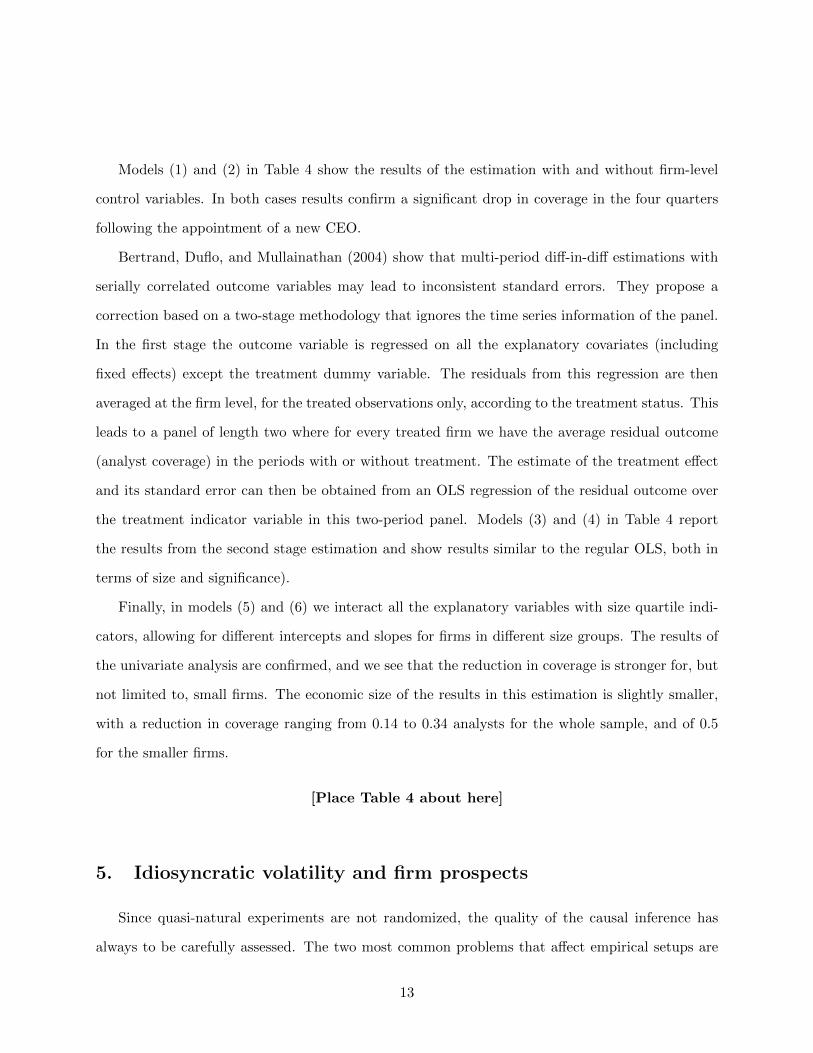
Models (1) and (2) in Table 4 show the results of the estimation with and without firm-level

control variables. In both cases results confirm a significant drop in coverage in the four quarters

following the appointment of a new CEO.

Bertrand, Duflo, and Mullainathan (2004) show that multi-period diff-in-diff estimations with

serially correlated outcome variables may lead to inconsistent standard errors. They propose a

correction based on a two-stage methodology that ignores the time series information of the panel.

In the first stage the outcome variable is regressed on all the explanatory covariates (including

fixed effects) except the treatment dummy variable. The residuals from this regression are then

averaged at the firm level, for the treated observations only, according to the treatment status. This

leads to a panel of length two where for every treated firm we have the average residual outcome

(analyst coverage) in the periods with or without treatment. The estimate of the treatment effect

and its standard error can then be obtained from an OLS regression of the residual outcome over

the treatment indicator variable in this two-period panel. Models (3) and (4) in Table 4 report

the results from the second stage estimation and show results similar to the regular OLS, both in

terms of size and significance).

Finally, in models (5) and (6) we interact all the explanatory variables with size quartile indi-

cators, allowing for different intercepts and slopes for firms in different size groups. The results of

the univariate analysis are confirmed, and we see that the reduction in coverage is stronger for, but

not limited to, small firms. The economic size of the results in this estimation is slightly smaller,

with a reduction in coverage ranging from 0.14 to 0.34 analysts for the whole sample, and of 0.5

for the smaller firms.

[Place Table 4 about here]

5. Idiosyncratic volatility and firm prospects

Since quasi-natural experiments are not randomized, the quality of the causal inference has

always to be carefully assessed. The two most common problems that affect empirical setups are

13

reverse-causality and spurious correlation created by some unobserved quantity. While the first

issue is unlikely to be relevant in our setting (its hard to argue that a reduction in the number of

analysts following a firm is the direct cause of a CEO turnover) the second could be problematic.

Specifically one could argue that both our outcome and treatment variable are caused by negative

prospects for the company.

On the one side McNichols and O’Brien (1997) argue that analysts are more likely to cover

firms with positive prospects in order to maximize brokerage revenues and Scherbina (2008) shows

that a drop in analyst coverage successfully predicts underperformance. On the other side we

know that CEO turnover is inversely related to firm past performance (Coughlan and Schmidt,

1985; Warner, Watts, and Wruck, 1988; Barro and Barro, 1990; Kaplan, 1994b,a) as investors learn

about managerial ability from stock returns (Bushman, Dai, and Wang, 2010; Pan et al., 2015).

Finally Pan et al. (2015) show that idiosyncratic volatility increases around CEO turnovers while

Ang et al. (2006) and Ang et al. (2009) document a negative correlation between idiosyncratic

volatility and future stock returns8.

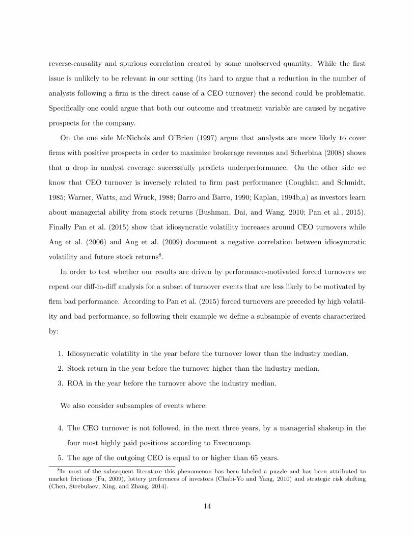
In order to test whether our results are driven by performance-motivated forced turnovers we

repeat our diff-in-diff analysis for a subset of turnover events that are less likely to be motivated by

firm bad performance. According to Pan et al. (2015) forced turnovers are preceded by high volatil-

ity and bad performance, so following their example we define a subsample of events characterized

by:

1. Idiosyncratic volatility in the year before the turnover lower than the industry median.

2. Stock return in the year before the turnover higher than the industry median.

3. ROA in the year before the turnover above the industry median.

We also consider subsamples of events where:

4. The CEO turnover is not followed, in the next three years, by a managerial shakeup in the

four most highly paid positions according to Execucomp.

5. The age of the outgoing CEO is equal to or higher than 65 years.

8In most of the subsequent literature this phenomenon has been labeled a puzzle and has been attributed tomarket frictions (Fu, 2009), lottery preferences of investors (Chabi-Yo and Yang, 2010) and strategic risk shifting(Chen, Strebulaev, Xing, and Zhang, 2014).

14

Panel A of Table 5 shows that our results are confirmed in this subsample. All the diff-in-diff

estimators have a negative sign indicating a drop in analyst coverage after an exogenous CEO

turnover. We also see that, while the size of the effect varies in the different subsamples, it is

generally economically relevant.

A possible concern with this results is that analysts my react to expected, rather than realized,

performance. In other words, conditioning our estimation on positive performance in the pre-

event period may not be sufficient to weed out the cases where the drop in coverage may be

motivated by performance rather than uncertainty. To address this issue we repeat the experiment

by conditioning on post-event positive performance of the firm (using the same three measures

outlined above but measured on the four quarters following the installation of the new CEO)9

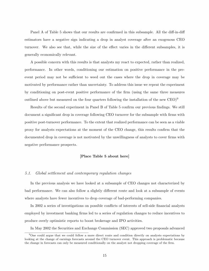
Results of the second experiment in Panel B of Table 5 confirm our previous findings. We still

document a significant drop in coverage following CEO turnover for the subsample with firms with

positive post-turnover performance. To the extent that realized performance can be seen as a viable

proxy for analysts expectations at the moment of the CEO change, this results confirm that the

documented drop in coverage is not motivated by the unwillingness of analysts to cover firms with

negative performance prospects.

[Place Table 5 about here]

5.1. Global settlement and contemporary regulation changes

In the previous analysis we have looked at a subsample of CEO changes not characterized by

bad performance. We can also follow a slightly different route and look at a subsample of events

where analysts have fewer incentives to drop coverage of bad-performing companies.

In 2002 a series of investigations on possible conflicts of interests of sell-side financial analysts

employed by investment banking firms led to a series of regulation changes to reduce incentives to

produce overly optimistic reports to boost brokerage and IPO activities.

In May 2002 the Securities and Exchange Commission (SEC) approved two proposals advanced

9One could argue that we could follow a more direct route and condition directly on analysts expectations bylooking at the change of earnings forecasts around the CEO turnover event. This approach is problematic becausethe change in forecasts can only be measured conditionally on the analyst not dropping coverage of the firm.

15

by the National Association of Securities Dealers (Rule 2711) and the New York Stock Exchange

(modified Rule 472). Among their provisions, these rules require all analyst research reports to

display the percentage of the issuing firms recommendations that are buys, holds, and sells.

In December 2002 the SEC announced the Global Analyst Research Settlement involving ten

U.S. investment firms that engaged in actions and practices that led to the inappropriate influence

of their research analysts by their investment bankers. The firms involved agreed to introduce a

series of organizational changes in order to separate research and investment banking. Although this

settlement only involved directly ten large institutions, its provisions became industry standards.

Under the new regulatory regime the incentives to cover stocks with positive prospects hypoth-

esized by McNichols and O’Brien (1997) is somewhat reduced10. Moreover, with this augmented

transparency enforced by Rule 2711 and Rule 472, analysts have to cover stocks with negative

prospects in order to maintain their credibility. Barber et al. (2006) document a dramatic shift in

the distribution of recommendations, with Buy recommendations dropping from 60% to 45% and

Sell recommendations changing from 5% to 15%. Kadan et al. (2009) report similar numbers and

also show that the effect is stronger for affiliated analysts (whose employer has business relations

with the covered firm).

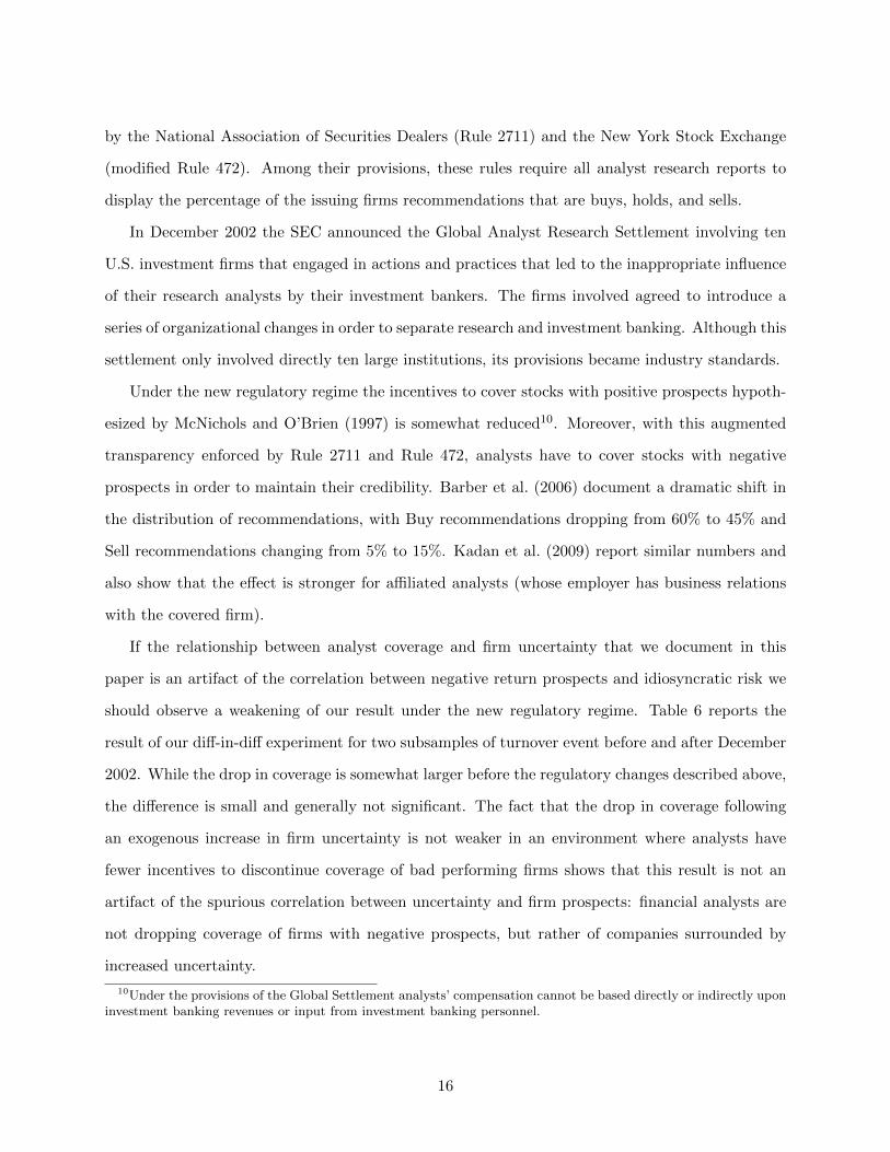
If the relationship between analyst coverage and firm uncertainty that we document in this

paper is an artifact of the correlation between negative return prospects and idiosyncratic risk we

should observe a weakening of our result under the new regulatory regime. Table 6 reports the

result of our diff-in-diff experiment for two subsamples of turnover event before and after December

2002. While the drop in coverage is somewhat larger before the regulatory changes described above,

the difference is small and generally not significant. The fact that the drop in coverage following

an exogenous increase in firm uncertainty is not weaker in an environment where analysts have

fewer incentives to discontinue coverage of bad performing firms shows that this result is not an

artifact of the spurious correlation between uncertainty and firm prospects: financial analysts are

not dropping coverage of firms with negative prospects, but rather of companies surrounded by

increased uncertainty.

10Under the provisions of the Global Settlement analysts’ compensation cannot be based directly or indirectly uponinvestment banking revenues or input from investment banking personnel.

16

[Place Table 6 about here]

6. Alternative shocks to uncertainty

Here we test the robustness of our results by examining alternative sources of shocks to uncer-

tainty. While we do not claim that these experiments enjoy the same level of exogeneity as CEO

turnovers, nonetheless they show that the drop in analyst coverage following an increase in uncer-

tainty of firm prospects is indeed general. As additional sources of uncertainty we consider the filing

of a securities class action where the firm is listed as defendant and three industry-specific shocks

that increased the uncertainty on the prospects of firms operating in the corresponding industries.

6.1. Securities Class Action

A securities class action is a lawsuit filed by investors who bought or sold a companys securities

and claim they suffered economic injury as a result of violations of securities laws. While the filing

of a class action has a predictable negative impact on the stock price of the firm (Griffin, Grundfest,

and Perino, 2000) the long term effects on the company are quite uncertain. Cheng, Huang, Li, and

Lobo (2010) show that on a sample of 1,213 lawsuit filed between 1996 and 2005, the dismissal rate,

i.e., the percentage of cases that were dismissed by the court without any negative consequence for

the defendant, was 37%. Comolli and Starykh (2015) report that, on a more recent sample of cases

filed and resolved between 2000 and 2014, a motion to dismiss was filed in 95% of the cases. Out

of these, the motion was granted in 48% of the cases (in addition to 8% of cases where the plaintiff

voluntary dismissed the claim). The authors also show a high degree of variation in the size of the

settlement for cases that are not dismissed.

In such a situation, it is fair to assume that investors, especially those that are not involved

in the class action, would express a strong demand for firm-specific information. Is the litigation

going to affect the long term growth prospects of the firm? Does the drop in market price at the

filing date make the stock attractive?

Using a sample of securities class actions filed from 1995 to 2013 we analyze the variation of

analyst coverage around the filing date for the defendants compared to a control sample of matched

17

firms. Since the event has a first-order effect on the market price of the stock we limit our matching

strategies to those firms for which we can build a control sample with comparable characteristics,

including return and turnover in the announcement quarter.

We take class actions data from the Stanford Law School Securities Class Action Clearinghouse,

and after matching with our sample we obtain 664 events.

Table 7 reports the results of a diff-in-diff analysis where we compare the change in analyst

coverage (quarter t + 4 minus quarter t − 4) for the firms named as defendants in securities class

actions to the change in coverage for a control sample of similar observations. Each firm/quarter in

the treatment sample is matched with the observation from the same quarter and industry closer

for Mahalanobis distance or propensity score based on the complete set of control variables used

in our main experiment (among which, turnover and excess return in the announcement quarter).

Results show a drop in analysts between 1 and 1.3 units, stronger than what measured in our main

experiment. This larger magnitude may be due to the fact that this event has a more directional

impact on expectations than the CEO turnover11. Figure 3 shows that both our control samples

satisfy the parallel trends assumption.

[Place Table 7 about here]

[Place Figure 3 about here]

While we cannot claim that this experiment is as strong and exogenous as our main one, we

think its fair to say that it offers a valuable corroboration. We show that coverage tends to drop

after a variety of firm-specific events that increase the uncertainty surrounding the company.

6.2. Industry Shocks

Lastly, we consider the fact that uncertainty surrounding a firm (or a group of firms) may

emerge from non-firm-specific events. Here we consider three different industry-related shocks that

for a variety of reason make the prospects of firms in the affected industries more uncertain.

11It is important to note that we match treatment and control observations by excess return in the announcementquarter so we control for the negative effect on firm prospects anticipated by investors at the time of the filing.Moreover Comolli and Starykh (2015) show that only 12% of cases are resolved (settled or dismissed) within the first12 months after the filing so it is unlikely that our result is affected by the resolution of the case.

18

The first event that we consider is Hurricane Katrina in August 2005 and its effect on insurance

companies. This hurricane is considered by far the most destructive extreme weather event in the

US history, with an estimated property damage of 108 b$ (Blake, Landsea, and Gibney, 2011). As

a comparison, the second most destructive storm (Sandy, October 2012) caused estimated damages

for 50 b$.

Assessing the impact on individual insurance companies of such an unprecedented amount of

potential claims is intrinsically complicated. Analysts would need to know not only the exact expo-

sure of the individual company to rather specific geographical areas but also the specificities of the

insured events. In the two years following the disaster, the media reported a number of controversies

on contentious damage assessments that spurred a number of lawsuits and class actions.

We argue that in the aftermath of this event, the uncertainty surrounding insurance companies

in the US would increase. Analysts covering insurance companies will be pressed to update their

estimates while, at the same time, facing an increased uncertainty.

The second event that we consider is the default of Lehman Brothers in September 2008. While

we acknowledge that this event had a clearly systemic dimension, it is reasonable to assume that

the uncertainty was particularly strong for financial firms and banks. Uncertainty not only about

the financial strength of individual institutions but also about future government interventions and

possible regulatory changes.

Lastly, we consider the bankruptcy of Enron in December 2001. At the time this was by far

the largest bankruptcy in history with 63.4 b$ of pre-filing assets, and came only months after the

demise of another energy company (Pacific Gas and Electric Co.) operating in the same market.

Subsequent investigation by the Federal Energy Regulatory Commission would link these cases in

an industry-wide investigation of what is today commonly known as the Western Energy Crisis

(Commission et al., 2003). According to later accounts of the fact, it seems that this collapse

was largely unanticipated both by analysts and by the public at large (Dyck and Zingales, 2003),

leading to the demise of one of the, until then, most reputable auditing firms in the world. We

argue that this collapse increased the uncertainty surrounding other companies operating in the

same industry and with similar business models.

Here we argue that these events increased the uncertainty surrounding the prospects of affected

19

firms. Since we are dealing with industry-related shocks, this assumption needs empirical verifica-

tion. We can provide a partial proof by looking at the change in idiosyncratic volatility in the year

after the event, compared with the year before. To test whether these events induced shocks in

idiosyncratic volatility of the affected firms, we run the following diff-in-diff regression

IdiosyncraticV arit = α+ βAffected it +Quartert + Firmi + ε (2)

Where Affected is the interaction between the indicator variables for the affected firms and the

time fixed effects for the four quarters after the event. We also estimate an alternative version of

this model where we replace firm fixed effects with industry fixed effects.

For the Katrina and the Lehman events we define affected companies (insurance companies and

banks respectively) based on the Fama and French 49 classification (number 45 and 46 respectively),

while for the Enron event we define affected companies those with SIC4 codes in the 4900-4932

range.

Results in Table 8 show that all three crisis events are associated with highly significant increases

in idiosyncratic volatility (as defined both by the single index or the 4-Factor model).

[Place Table 8 about here]

Now that we have established our exogenous shocks we can observe the evolution of analyst

coverage around the three events running a modified version of the diff-in-diff model where we add

firm-level controls.

Ln(Coverageit) = α+ βAffected it + γZit +Quartert + Firmi + ε (3)

Results in Table 9 show that when we control for other factors affecting coverage decisions we

see a clear reduction in coverage associated with our crisis events. The size of the reduction varies

20

across events, but is always relevant: estimated coefficients indicate a drop of 1.4–1.5 analysts

after the Enron bankruptcy, 0.4–0.6 analysts after hurricane Katrina and 0.3–0.6 analysts after the

Lehman collapse.

[Place Table 9 about here]

While quite different in spirit from our main experiment, this last analysis offers additional

corroboration of our main hypothesis. Financial analysts react to an increase in uncertainty sur-

rounding the prospects of a firm by discontinuing coverage.

7. Career Concerns and Analysts Characteristics

In the previous paragraph we have provided evidence that the number of analysts following a

company drops after an exogenous increase in the uncertainty surrounding the prospects of the

company.

Here we analyze possible reasons for this behavior by looking at the individual characteristics

of analysts who dropped coverage after the appointment of a new CEO. The analysis will focus on

all the analysts who were covering a stock prior to the turnover event (i.e. analysts who issued

an EPS forecast in the six months prior to the event) and whose forecast is included in the IBES

Stopped Estimate File within twelve months of the event.

According to IBES, the Stopped Estimate file contain forecasts that have been withdrawn by

the estimator or that have not been updated or confirmed for 180 days. Estimates contained in

this file may have been stopped for a variety of undisclosed reasons. For example, a broker may

routinely stop estimates when the issuing analyst leaves the firm, or an estimate could be dropped

and immediately replaced by a new estimate, perhaps issued on behalf of the same broker by a

different analyst. We apply a series of filters to reduce our sample to a collection of meaningful

decisions to interrupt coverage of a firm. Specifically we drop observations where:

• The analyst does not issue any other forecast for the same broker in the year following the

coverage interruption. We want to avoid cases where the estimate has been stopped because

the analyst has retired or has moved to another broker.

21

• The broker issues a new forecast for the same company within three months from the in-

terruption. We want to avoid cases where the broker has simply replaced an old estimate

with a new one. While brokers can routinely update existing estimates, one could imagine a

situation where a broker decides to assign the company to a different analyst, and thus the

old estimate is retired and a new one is immediately issued. The three months gap ensures

that we are analysing a situation where there is a significant interruption of coverage that

spans at least one full fiscal quarter.

• The broker does not issue any new forecast in the year following the coverage interruption.

We want to avoid situations where a broker drops all its existing forecasts before merging

with a rival or leaving the industry.

In all these cases, it is likely that the forecast has been included in the stopped file for reasons

different from the conscious decision that we are trying to model here. A natural control sample for

this analysis is provided by all the analysts who were covering firms affected by the CEO turnover

events and whose forecast is not included in the Stopped Estimate File. These are the analysts who

have not discontinued coverage in spite of the increase in uncertainty. Our final sample contains

3,789 stopped estimates (from 2,399 individual analysts) and 35,297 retained estimates (from 7,449

analysts). In our selection criteria we impose that the stopped estimate cannot be followed by a

new forecast (from the same broker) within three months. From the length of coverage interruption

we see that for 59.5% of the stopped estimates there is no record of a new forecast in the sample

period, indicating that the broker has dropped coverage in a permanent way. For the remaining

events we observe an interruption shorter than one year in 26.9% of cases, and longer than one year

in the remaining 13.6%. When coverage is resumed, the new forecast is issued by the same analyst

in 58.3% of the cases and by a different analyst in the remaining 41.7%.

7.1. Analysts Characteristics

The literature on herding behavior provides a useful guide to measure reputational and career

concerns. Hong et al. (2000) show that analysts who produce erroneous forecasts may face negative

career outcomes. Analysts may react to this termination risk by playing safe, that is by issuing

forecast close to the prevailing consensus. Here we argue that dropping coverage of a firm is an

22

alternative response to the same career and reputational concerns. From the existing literature on

herding we extract a number of characteristics related to four areas: a) experience of the analyst,

b) workload, c) reputation and d) risk aversion.

Experience

The first three variables are related to the working experience of the analyst and capture the

idea, common in the financial literature, that professionals in early stages of their career face

stronger reputational risk. Hong et al. (2000) show that inexperienced analysts are more likely

to suffer negative career outcomes as a result of inaccurate forecasts. The same phenomenon has

been documented in other segments of the financial industry. For example, Chevalier, Ellison,

et al. (1999) show that termination risk for mutual fund managers is more performance-sensitive

for younger portfolio managers. Clement and Tse (2005), in a slightly different context, show that

analysts with less experience (both general and firm-specific) exhibit stronger herding behavior.

The authors interpret this result as a signal of stronger reputational concerns. Based on this

research we record the following three variables:

• General Experience is the time since the first forecast ever issued by the analyst.

• Firm Experience is the time since the first forecast the analyst has produced for the specific

company.

• Tenure is the time since the first forecast of the analyst with the present brokerage house.

Here we expect these three dimensions of professional experience to be associated with lower prob-

ability of dropping coverage of a company after a turnover event.

These measures pose a possible empirical challenge as they are, by construction, non-stationary

in time. To avoid spurious results we follow Clement and Tse (2005) and Hilary and Hsu (2013)

and normalize the variables so that each analyst is measured against his/her other peers covering

the same firm. Specifically, we rank all the analysts following a given firm before the CEO turnover

according to each raw measure (for example General Experience) and define the normalized measure

as:

Normalized Measure =(rank − 1)

(N − 1)(4)

23

Where N is the number of analysts covering the firm. With this measure the least experienced

analyst following a firm will have a score of zero while the most experienced will have a score of

one.

Workload The second two variables capture the idea that analysts who have to cover a large

number of firms (or firms operating in a large number of different industries) have less time to

dedicate to each individual forecast and develop more superficial knowledge of each individual firm.

Clement and Tse (2005) show that analysts who cover a large number of firms (or firms in very

diverse industries) are more likely to exhibit herding behavior as they know less of any specific firm

or industrial context, and thus face higher risk of making costly mistakes. Based on this research

we build the following two variables:

• Companies is a measure of workload and is defined as the (normalized) number of firms

covered by the analyst in the current year.

• Industries is a measure of analyst specialization and, to a certain extent, workload, and

is defined as the (normalized) number of different industries covered by the analyst in the

current year (following the Fama and French 12 categorization).

Our expectation is that analysts covering multiple firms or industries will be more likely to drop

coverage of a specific firm following an increase in uncertainty.

Reputation We also build two variables to proxy for analyst reputation. Analysts with a strong

reputation are less likely to experience negative career outcomes after a wrong estimate. Jackson

(2005) shows that reputation is strongly increasing in the size of the broker and argues that this

result is consistent with larger brokers employing better analysts and having more resources at their

disposal. Similarly Clement and Tse (2005) find that brokerage size and past accuracy are associated

with lower herding behavior, a sign of lower reputational concerns. Based on this research we build

the following two measures:

• Broker Size is the (normalized) size of the brokerage firm in terms of analysts employed in

the year.

24

• Accuracy is the average relative accuracy of the analyst over his/her entire career.

In order to build this last measure, we follow Hilary and Hsu (2013) and consider, for every firm

and fiscal period, the first forecast produced by each analyst covering the firm, rank them from the

least to the most accurate (based on the absolute distance from the realized EPS) and calculate

the normalized ranking. Accuracy is defined as the average ranking over the whole career of the

analyst, thus considering it as a time-invariant attribute. We expect analysts working for larger

brokerage houses and analysts with stronger track records in terms of accuracy to have a lower

probability of dropping coverage of firms with uncertain prospects.

Risk Aversion Finally, we model analysts risk aversion looking at the average relative boldness

of their forecasts. Several theories link reputational concerns to herding behavior (Scharfstein and

Stein, 1990; Trueman, 1994), and Hong et al. (2000) show that bold forecasts increase the likelihood

of termination for financial analysts. Here we argue that analysts who on average produce bolder

forecasts are less afraid of taking risks (either because of a lower risk aversion or a higher assessment

of their own ability) and thus show lower reputational and career concerns.

Following prior research, we define Boldness as the absolute distance from the prevailing con-

sensus estimate and we measure the relative attribute with a ranking process similar to the one

used to build our accuracy measure.

We expect analysts with lower risk aversion (higher Boldness) to be less likely to drop coverage

after an exogenous increase of firm uncertainty.

Table 10 reports the correlation matrix between these analysts characteristics. The relationships

between the variables are consistent with existing literature: analysts working for large brokers and

more experienced analysts are more accurate (Lim, 2001; Clement and Tse, 2005) and analysts

covering a large number of firms / industries tend to be less accurate and less bold (Clement and

Tse, 2005).

[Place Table 10 about here]

25

7.2. Career Concerns and stopped forecasts

In order to assess whether the decision to drop coverage of difficult firms is due to reputational

concerns we can look at differences in our proxy variables between analysts whose forecasts have

been stopped or not.

Results in Table 11 show that, in fact, dropped forecasts come from analysts with lower expe-

rience (both general, firm-specific and broker-specific), higher workload, weaker reputation (both

in terms of accuracy and size of their employer) and higher risk aversion (measured by the average

boldness of their forecasts). All these results are consistent with our hypothesis that the decision

to drop coverage of firms whose prospects have become more uncertain due to a crisis event is

due to reputational and career concerns: the same variables that, according to existing literature,

drive analysts to produce forecasts close to the prevailing consensus (i.e. to herd) also increase the

probability that the issued forecasts will be stopped in the aftermath of an exogenous increase of

the uncertainty surrounding the firm.

[Place Table 11 about here]

From previous research (and from Table 10) we know that our proxy variables are correlated,

and thus a multivariate analysis of the factors affecting the decision to drop coverage may be

more appropriate. We estimate the following logit model (with robust standard errors) where the

dependent variable is a dummy equal to one for the dropped forecasts.

Pr(Stopped) = logit−1(b0 + b1Experience+ b2Workload+ b3Reputation+ b4Boldness+ e) (5)

From the results of this estimation, we can see in Table 12 that all the findings of our univariate

analysis are confirmed: the probability of dropping coverage of a firm after the appointment of

a new CEO is higher for inexperienced analysts with a weaker reputation, higher workload and

higher risk-aversion. This indicates that reputational concerns significantly affect the probability

of dropping coverage when firm prospects become more unpredictable.

26

[Place Table 12 about here]

Since most of our covariates are correlated, quantifying the individual marginal effects can

be problematic. Table 13 reports realized frequency of dropped forecasts and average predicted

probability of dropping coverage (from model (6) in Table 12) for subsamples of observations with

low and high values of the different covariates, where low and high are defined as belonging to the

first and fifth quintile respectively. Among the more relevant results we can see, for example, that

the probability of discontinuing coverage is 2% lower for analysts with a long experience covering

the firm compared to analysts with limited experience. Given that the unconditional probability of

dropping coverage in our sample is 9.7%, this difference is substantial. Similarly, we can see that

an analyst with a strong reputation is 2.9% less likely to interrupt coverage than a colleague with

weaker reputation. Finally, we can observe that generalists (analysts covering a large number of

industries) are 2% more likely to interrupt coverage than specialists.

[Place Table 13 about here]

Overall, the results of our investigation around the behavior of individual financial analysts

around CEO turnover events introduced in the previous section shows that the decision to drop the

coverage of a firm whose prospects have become more uncertain is affected by a number of factors

that, according to previous research, are associated with reputational risk and career concerns.

8. Conclusion

In this paper we look at how reputational and career concerns affect coverage decisions by

financial analysts. Prior literature has shown that career success is tied to forecasting accuracy, so

when a firm becomes too difficult to cover due to a high level of uncertainty, analysts may decide

to drop coverage in order to avoid costly mistakes.

We observe analysts reaction to an exogenous increase in firm-specific uncertainty due to CEO

turnover, and show that in the twelve months after the appointment of the new CEO affected firms

experience a drop in coverage of 0.6–0.7 units compared to a control sample of similar companies.

This result is surprising if we consider that a change in CEO should not systematically lead to a

27

decrease in the demand of brokerage services.

In order to address the possible concern that our finding may simply capture the fact that

analysts do not like to cover firms with negative return prospects we confirm the result on a

subsample of turnover events less likely to be associated with bad return prospects for the firm. We

also show that our findings become stronger in a regime where analysts have stronger incentives to

cover firms with negative prospects (after the Global Analysts Settlement of 2002).

An additional concern is that our results may capture something specific to CEO turnovers. To

assess the general relevance of our findings we consider alternative sources of firm uncertainty. First

of all we look at securities class actions and show that, relative to a control sample of similar firms,

firms listed as defendants experience a drop in coverage of 1 to 1.3 analysts in the four quarters

after the filing. We then study industry-related shocks that are likely to increase uncertainty for all

the firms in the affected industries. We consider Hurricane Katrina for insurance companies, the

default of Lehman brothers for financial firms and the collapse of Enron for firms with a similar

business model, and show that affected firms experience a drop in coverage (compared to the

average unaffected firm) from 0.4 to 1.4 analysts. While we acknowledge that these experiments

do not enjoy the same level of exogeneity as the CEO turnovers, they nonetheless show that the

drop in analyst coverage following an increase in uncertainty of firm prospects is a general, and is

not limited to a specific type of event.

Finally, using data on individual forecasts we show that the probability of dropping coverage

after an exogenous increase in uncertainty is higher for less experienced and less reputable analysts,

for analysts who cover more firms and more industries and for analysts with higher risk aversion.

All these factors have been linked, in previous literature, to higher reputational and career concerns

and stronger herding behavior.

Taken altogether these results show that career concerns affect analysts activity in more than

one way. They not only make analysts forecasts less informative but also affect the choice of firms

that are covered. This highlights an additional dimension to the endogeneity of analyst coverage

that has to be properly addressed in order to correctly assess the effect of financial analysts on

stock returns and managerial behavior.

28

References

Abadie, A., Drukker, D., Herr, J. L., Imbens, G. W., et al., 2004. Implementing matching estimators

for average treatment effects in stata. Stata journal 4, 290–311.

Abadie, A., Imbens, G. W., 2006. Large sample properties of matching estimators for average

treatment effects. Econometrica 74, 235–267.

Abadie, A., Imbens, G. W., 2012. Bias-corrected matching estimators for average treatment effects.

Journal of Business & Economic Statistics 29, 1–11.

Anantharaman, D., Zhang, Y., 2011. Cover me: Managers’ responses to changes in analyst coverage

in the post-regulation fd period. The Accounting Review 86, 1851–1885.

Ang, A., Hodrick, R. J., Xing, Y., Zhang, X., 2006. The cross-section of volatility and expected

returns. The Journal of Finance 61, 259–299.

Ang, A., Hodrick, R. J., Xing, Y., Zhang, X., 2009. High idiosyncratic volatility and low returns:

International and further us evidence. Journal of Financial Economics 91, 1–23.

Asquith, P., Mikhail, M. B., Au, A. S., 2005. Information content of equity analyst reports. Journal

of financial economics 75, 245–282.

Barber, B. M., Lehavy, R., McNichols, M., Trueman, B., 2006. Buys, holds, and sells: The distri-

bution of investment banks? stock ratings and the implications for the profitability of analysts?

recommendations. Journal of accounting and Economics 41, 87–117.

Barro, J. R., Barro, R. J., 1990. Pay, performance, and turnover of bank ceos. Journal of Labor

Economics pp. 448–481.

Bertrand, M., Duflo, E., Mullainathan, S., 2004. How much should we trust differences-in-differences

estimates? Quarterly Journal of Economics 119, 249–275.

Bhushan, R., 1989. Firm characteristics and analyst following. Journal of Accounting and Eco-

nomics 11, 255–274.

29

Blake, E. S., Landsea, C., Gibney, E. J., 2011. The deadliest, costliest, and most intense united

states tropical cyclones from 1851 to 2010 (and other frequently requested hurricane facts). NOAA

Technical Memorandum NWS NHC-6, National Oceanic and Atmospheric Administration.

Brown, L. D., Call, A. C., Clement, M. B., Sharp, N. Y., 2015. Inside the black box of sell-side

financial analysts. Journal of Accounting Research 53, 1–47.

Bushman, R., Dai, Z., Wang, X., 2010. Risk and ceo turnover. Journal of Financial Economics 96,

381–398.

Bushman, R. M., Piotroski, J. D., Smith, A. J., 2005. Insider trading restrictions and analysts’

incentives to follow firms. The Journal of Finance 60, 35–66.

Chabi-Yo, F., Yang, J., 2010. Idiosyncratic coskewness and equity return anomalies. Bank of Canada

Working Paper .

Chan, K., Hameed, A., 2006. Stock price synchronicity and analyst coverage in emerging markets.

Journal of Financial Economics 80, 115–147.

Chen, Z., Strebulaev, I. A., Xing, Y., Zhang, X., 2014. Strategic risk shifting and the idiosyncratic

volatility puzzle. Rock Center for Corporate Governance at Stanford University Working Paper

.

Cheng, C. A., Huang, H. H., Li, Y., Lobo, G., 2010. Institutional monitoring through shareholder

litigation. Journal of Financial Economics 95, 356–383.

Chevalier, J., Ellison, G., et al., 1999. Career concerns of mutual fund managers. The Quarterly

Journal of Economics 114, 389–432.

Clement, M. B., Tse, S. Y., 2005. Financial analyst characteristics and herding behavior in fore-

casting. The Journal of finance 60, 307–341.

Commission, F. E. R., et al., 2003. Final report on price manipulation in western markets, fact-

finding investigation of potential manipulation of electric and natural gas prices. Tech. Rep.

Docket No. PA02-2-000.

30

Comolli, R., Starykh, S., 2015. Recent trends in securities class action litigation: 2014 full-year

review. National Economic Research Association, New York .

Coughlan, A. T., Schmidt, R. M., 1985. Executive compensation, management turnover, and firm

performance: An empirical investigation. Journal of Accounting and Economics 7, 43–66.

Derrien, F., Kecskes, A., 2013. The real effects of financial shocks: Evidence from exogenous changes

in analyst coverage. The Journal of Finance 68, 1407–1440.

Dyck, A., Zingales, L., 2003. The bubble and the media. In: Cornelius, P., Kogut, B. M. (eds.),

Corporate governance and capital flows in a global economy , Oxford University Press New York,

NY, pp. 83–104.

Fu, F., 2009. Idiosyncratic risk and the cross-section of expected stock returns. Journal of Financial

Economics 91, 24–37.

Giroud, X., Mueller, H. M., 2010. Does corporate governance matter in competitive industries?

Journal of Financial Economics 95, 312–331.

Griffin, P. A., Grundfest, J., Perino, M. A., 2000. Stock price response to news of securities fraud

litigation: Market efficiency and the slow diffusion of costly information. Stanford Law and

Economics Olin Working Paper .

He, J. J., Tian, X., 2013. The dark side of analyst coverage: The case of innovation. Journal of

Financial Economics 109, 856–878.

Hilary, G., Hsu, C., 2013. Analyst forecast consistency. The Journal of Finance 68, 271–297.

Hong, H., Kubik, J. D., 2003. Analyzing the analysts: Career concerns and biased earnings forecasts.

The Journal of Finance 58, 313–351.

Hong, H., Kubik, J. D., Solomon, A., 2000. Security analysts’ career concerns and herding of

earnings forecasts. The Rand journal of economics 31, 121–144.

Irani, R. M., Oesch, D., 2016. Analyst coverage and real earnings management: Quasi-experimental

evidence. Journal of Financial and Quantitative Analysis (JFQA), Forthcoming .

31

Jackson, A. R., 2005. Trade generation, reputation, and sell-side analysts. The Journal of Finance

60, 673–717.

Kadan, O., Madureira, L., Wang, R., Zach, T., 2009. Conflicts of interest and stock recommenda-

tions: The effects of the global settlement and related regulations. Review of Financial Studies

22, 4189–4217.

Kaplan, S. N., 1994a. Top executive rewards and firm performance: A comparison of japan and the

united states. Journal of Political Economy 102, 510–546.

Kaplan, S. N., 1994b. Top executives, turnover, and firm performance in germany. Journal of Law,

Economics, & Organization pp. 142–159.

Kim, M. S., Zapatero, F., 2011. Competitive compensation and dispersion in analysts’ recommen-

dations. Working Paper .

Lim, T., 2001. Rationality and analysts’ forecast bias. The Journal of Finance 56, 369–385.

Loh, R. K., Stulz, R. M., 2011. When are analyst recommendation changes influential? Review of

Financial Studies 24, 593–627.

McNichols, M., O’Brien, P. C., 1997. Self-selection and analyst coverage. Journal of Accounting

Research 35, 167–199.

Mola, S., Rau, P. R., Khorana, A., 2012. Is there life after the complete loss of analyst coverage?

The Accounting Review 88, 667–705.

Pan, Y., Wang, T. Y., Weisbach, M. S., 2015. Learning about ceo ability and stock return volatility.

Review of Financial Studies p. hhv014.

Piotroski, J. D., Roulstone, D. T., 2004. The influence of analysts, institutional investors, and

insiders on the incorporation of market, industry, and firm-specific information into stock prices.

The Accounting Review 79, 1119–1151.

Roll, R., 1988. R2. Journal of Finance 43, 541–566.

32

Scharfstein, D. S., Stein, J. C., 1990. Herd behavior and investment. The American Economic

Review pp. 465–479.

Scherbina, A., 2008. Suppressed negative information and future underperformance*. Review of

Finance 12, 533–565.

Shon, J., Young, S. M., 2011. Determinants of analysts dropped coverage decision: The role of

analyst incentives, experience, and accounting fundamentals. Journal of Business Finance &

Accounting 38, 861–886.

Stickel, S. E., 1992. Reputation and performance among security analysts. The Journal of Finance

47, 1811–1836.

Trueman, B., 1994. Analyst forecasts and herding behavior. Review of financial studies 7, 97–124.

Warner, J. B., Watts, R. L., Wruck, K. H., 1988. Stock prices and top management changes. Journal

of financial Economics 20, 461–492.

Yu, F. F., 2008. Analyst coverage and earnings management. Journal of Financial Economics 88,

245–271.

33

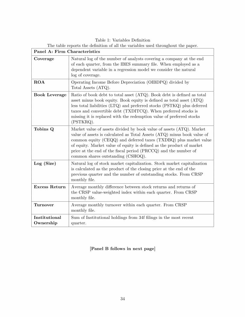
Table 1: Variables DefinitionThe table reports the definition of all the variables used throughout the paper.

Panel A: Firm Characteristics

Coverage Natural log of the number of analysts covering a company at the endof each quarter, from the IBES summary file. When employed as adependent variable in a regression model we consider the naturallog of coverage.

ROA Operating Income Before Depreciation (OIBDPQ) divided byTotal Assets (ATQ).

Book Leverage Ratio of book debt to total asset (ATQ). Book debt is defined as totalasset minus book equity. Book equity is defined as total asset (ATQ)less total liabilities (LTQ) and preferred stocks (PSTKQ) plus deferredtaxes and convertible debt (TXDITCQ). When preferred stocks ismissing it is replaced with the redemption value of preferred stocks(PSTKRQ).

Tobins Q Market value of assets divided by book value of assets (ATQ). Marketvalue of assets is calculated as Total Assets (ATQ) minus book value ofcommon equity (CEQQ) and deferred taxes (TXDBQ) plus market valueof equity. Market value of equity is defined as the product of marketprice at the end of the fiscal period (PRCCQ) and the number ofcommon shares outstanding (CSHOQ).

Log (Size) Natural log of stock market capitalization. Stock market capitalizationis calculated as the product of the closing price at the end of theprevious quarter and the number of outstanding stocks. From CRSPmonthly file.

Excess Return Average monthly difference between stock returns and returns ofthe CRSP value-weighted index within each quarter. From CRSPmonthly file.

Turnover Average monthly turnover within each quarter. From CRSPmonthly file.

Institutional Sum of Institutional holdings from 34f filings in the most recentOwnership quarter.

[Panel B follows in next page]

34

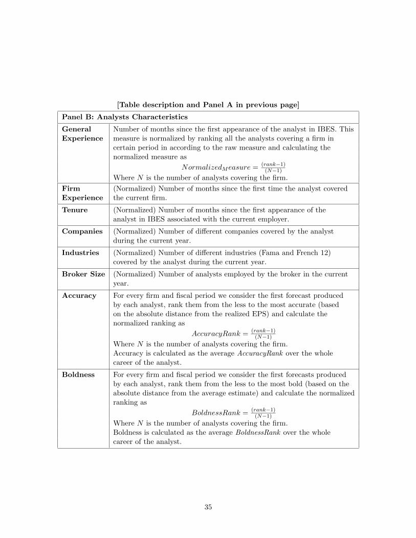
[Table description and Panel A in previous page]

Panel B: Analysts Characteristics

General Number of months since the first appearance of the analyst in IBES. ThisExperience measure is normalized by ranking all the analysts covering a firm in

certain period in according to the raw measure and calculating thenormalized measure as

NormalizedMeasure = (rank−1)(N−1)

Where N is the number of analysts covering the firm.

Firm (Normalized) Number of months since the first time the analyst coveredExperience the current firm.

Tenure (Normalized) Number of months since the first appearance of theanalyst in IBES associated with the current employer.

Companies (Normalized) Number of different companies covered by the analystduring the current year.

Industries (Normalized) Number of different industries (Fama and French 12)covered by the analyst during the current year.

Broker Size (Normalized) Number of analysts employed by the broker in the currentyear.

Accuracy For every firm and fiscal period we consider the first forecast producedby each analyst, rank them from the less to the most accurate (basedon the absolute distance from the realized EPS) and calculate thenormalized ranking as

AccuracyRank = (rank−1)(N−1)

Where N is the number of analysts covering the firm.Accuracy is calculated as the average AccuracyRank over the wholecareer of the analyst.

Boldness For every firm and fiscal period we consider the first forecasts producedby each analyst, rank them from the less to the most bold (based on theabsolute distance from the average estimate) and calculate the normalizedranking as

BoldnessRank = (rank−1)(N−1)

Where N is the number of analysts covering the firm.Boldness is calculated as the average BoldnessRank over the wholecareer of the analyst.

35

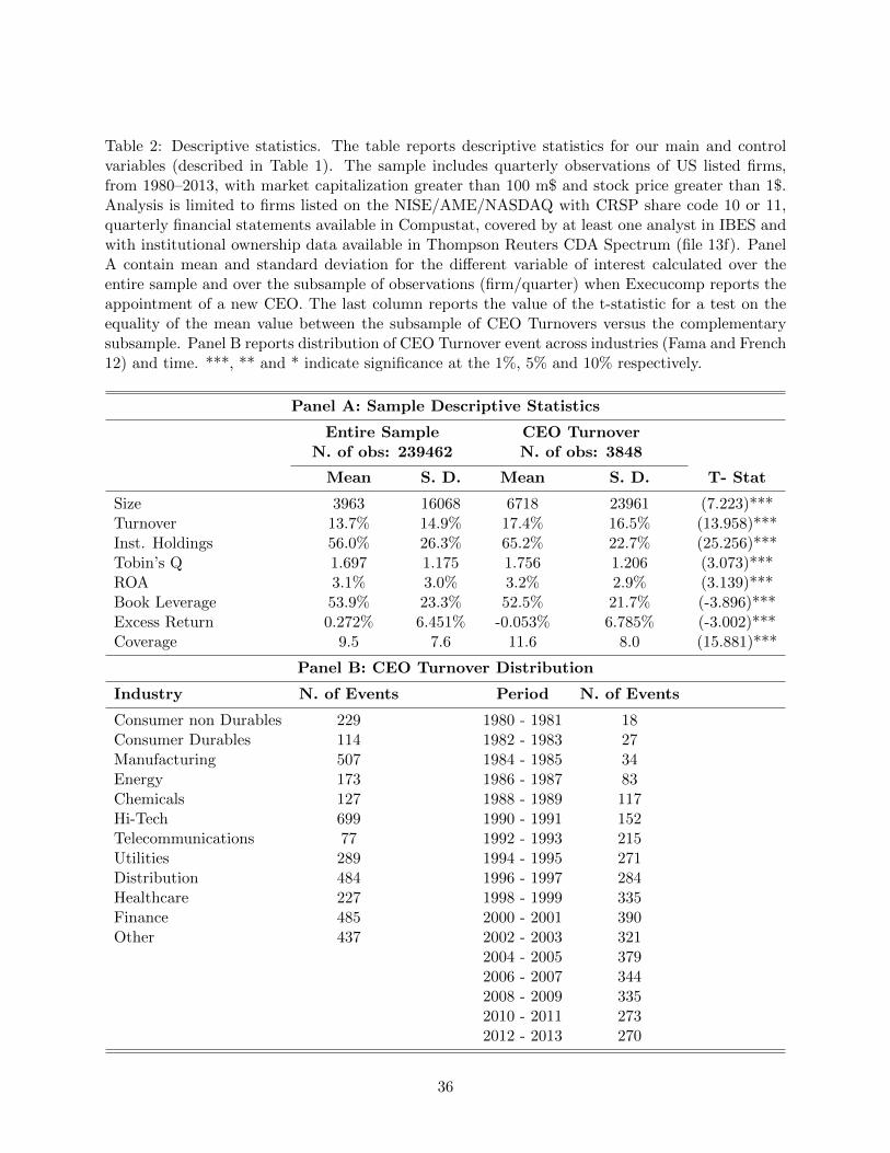
Table 2: Descriptive statistics. The table reports descriptive statistics for our main and controlvariables (described in Table 1). The sample includes quarterly observations of US listed firms,from 1980–2013, with market capitalization greater than 100 m$ and stock price greater than 1$.Analysis is limited to firms listed on the NISE/AME/NASDAQ with CRSP share code 10 or 11,quarterly financial statements available in Compustat, covered by at least one analyst in IBES andwith institutional ownership data available in Thompson Reuters CDA Spectrum (file 13f). PanelA contain mean and standard deviation for the different variable of interest calculated over theentire sample and over the subsample of observations (firm/quarter) when Execucomp reports theappointment of a new CEO. The last column reports the value of the t-statistic for a test on theequality of the mean value between the subsample of CEO Turnovers versus the complementarysubsample. Panel B reports distribution of CEO Turnover event across industries (Fama and French12) and time. ***, ** and * indicate significance at the 1%, 5% and 10% respectively.

Panel A: Sample Descriptive Statistics

Entire Sample CEO TurnoverN. of obs: 239462 N. of obs: 3848

Mean S. D. Mean S. D. T- Stat

Size 3963 16068 6718 23961 (7.223)***Turnover 13.7% 14.9% 17.4% 16.5% (13.958)***Inst. Holdings 56.0% 26.3% 65.2% 22.7% (25.256)***Tobin’s Q 1.697 1.175 1.756 1.206 (3.073)***ROA 3.1% 3.0% 3.2% 2.9% (3.139)***Book Leverage 53.9% 23.3% 52.5% 21.7% (-3.896)***Excess Return 0.272% 6.451% -0.053% 6.785% (-3.002)***Coverage 9.5 7.6 11.6 8.0 (15.881)***

Panel B: CEO Turnover Distribution

Industry N. of Events Period N. of Events

Consumer non Durables 229 1980 - 1981 18Consumer Durables 114 1982 - 1983 27Manufacturing 507 1984 - 1985 34Energy 173 1986 - 1987 83Chemicals 127 1988 - 1989 117Hi-Tech 699 1990 - 1991 152Telecommunications 77 1992 - 1993 215Utilities 289 1994 - 1995 271Distribution 484 1996 - 1997 284Healthcare 227 1998 - 1999 335Finance 485 2000 - 2001 390Other 437 2002 - 2003 321

2004 - 2005 3792006 - 2007 3442008 - 2009 3352010 - 2011 2732012 - 2013 270

36

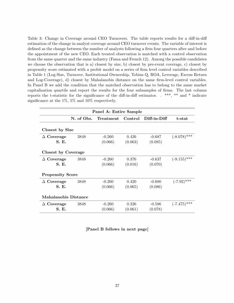
Table 3: Change in Coverage around CEO Turnovers. The table reports results for a diff-in-diffestimation of the change in analyst coverage around CEO turnover events. The variable of interest isdefined as the change between the number of analysts following a firm four quarters after and beforethe appointment of the new CEO. Each treated observation is matched with a control observationfrom the same quarter and the same industry (Fama and French 12). Among the possible candidateswe choose the observation that is a) closest by size, b) closest by pre-event coverage, c) closest bypropensity score estimated with a probit model on a series of firm level control variables describedin Table 1 (Log-Size, Turnover, Institutional Ownership, Tobins Q, ROA, Leverage, Excess Returnand Log-Coverage), d) closest by Mahalanobis distance on the same firm-level control variables.In Panel B we add the condition that the matched observation has to belong to the same marketcapitalization quartile and report the results for the four subsamples of firms. The last columnreports the t-statistic for the significance of the diff-in-diff estimator. . ***, ** and * indicatesignificance at the 1%, 5% and 10% respectively.

Panel A: Entire Sample

N. of Obs. Treatment Control Diff-in-Diff t-stat

Closest by Size

∆ Coverage 3848 -0.260 0.426 -0.687 (-8.078)***S. E. (0.066) (0.063) (0.085)

Closest by Coverage

∆ Coverage 3848 -0.260 0.376 -0.637 (-9.155)***S. E. (0.066) (0.016) (0.070)

Propensity Score

∆ Coverage 3848 -0.260 0.420 -0.680 (-7.92)***S. E. (0.066) (0.065) (0.086)

Mahalanobis Distance

∆ Coverage 3848 -0.260 0.326 -0.586 (-7.475)***S. E. (0.066) (0.061) (0.078)

[Panel B follows in next page]

37

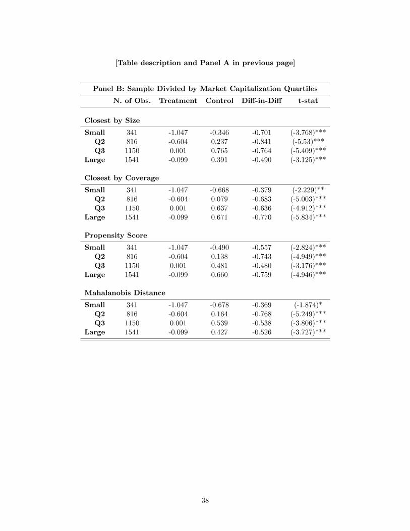
[Table description and Panel A in previous page]

Panel B: Sample Divided by Market Capitalization Quartiles

N. of Obs. Treatment Control Diff-in-Diff t-stat

Closest by Size

Small 341 -1.047 -0.346 -0.701 (-3.768)***Q2 816 -0.604 0.237 -0.841 (-5.53)***Q3 1150 0.001 0.765 -0.764 (-5.409)***

Large 1541 -0.099 0.391 -0.490 (-3.125)***

Closest by Coverage

Small 341 -1.047 -0.668 -0.379 (-2.229)**Q2 816 -0.604 0.079 -0.683 (-5.003)***Q3 1150 0.001 0.637 -0.636 (-4.912)***

Large 1541 -0.099 0.671 -0.770 (-5.834)***

Propensity Score

Small 341 -1.047 -0.490 -0.557 (-2.824)***Q2 816 -0.604 0.138 -0.743 (-4.949)***Q3 1150 0.001 0.481 -0.480 (-3.176)***

Large 1541 -0.099 0.660 -0.759 (-4.946)***

Mahalanobis Distance

Small 341 -1.047 -0.678 -0.369 (-1.874)*Q2 816 -0.604 0.164 -0.768 (-5.249)***Q3 1150 0.001 0.539 -0.538 (-3.806)***

Large 1541 -0.099 0.427 -0.526 (-3.727)***

38

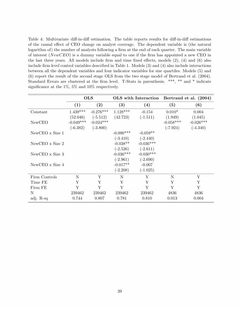
Table 4: Multivariate diff-in-diff estimation. The table reports results for diff-in-diff estimationsof the causal effect of CEO change on analyst coverage. The dependent variable is (the naturallogarithm of) the number of analysts following a firm at the end of each quarter. The main variableof interest (NewCEO) is a dummy variable equal to one if the firm has appointed a new CEO inthe last three years. All models include firm and time fixed effects, models (2), (4) and (6) alsoinclude firm level control variables described in Table 1. Models (3) and (4) also include interactionsbetween all the dependent variables and four indicator variables for size quartiles. Models (5) and(6) report the result of the second stage OLS from the two stage model of Bertrand et al. (2004).Standard Errors are clustered at the firm level. T-Stats in parenthesis. ***, ** and * indicatesignificance at the 1%, 5% and 10% respectively.

OLS OLS with Interaction Bertrand et al. (2004)

(1) (2) (3) (4) (5) (6)

Constant 1.439*** -0.276*** 1.128*** -0.154 0.010* 0.004(52.046) (-5.512) (42.723) (-1.511) (1.949) (1.045)

NewCEO -0.049*** -0.024*** -0.058*** -0.026***(-6.382) (-3.800) (-7.924) (-4.340)

NewCEO x Size 1 -0.090*** -0.059**(-3.410) (-2.440)

NewCEO x Size 2 -0.038** -0.036***(-2.526) (-2.611)

NewCEO x Size 3 -0.036*** -0.030***(-2.961) (-2.690)

NewCEO x Size 4 -0.017** -0.007(-2.208) (-1.025)

Firm Controls N Y N Y N YTime FE Y Y Y Y Y YFirm FE Y Y Y Y Y YN 239462 239462 239462 239462 4836 4836adj. R-sq 0.744 0.807 0.781 0.810 0.013 0.004

39

Table 5: Exogenous CEO Turnovers. The table reports results for a diff-in-diff estimation of thechange in analyst coverage around CEO turnovers for a subsample of events characterized by ahigher likelihood of exogeneity. In Panel A we consider events with: a) Pre-event idiosyncraticvolatility below industry median; b) Pre-event equity return above industry median; c) Pre-eventROA above industry median; d) All three of the previous conditions; e) Absence of managerialshakeup in the three years after the event; f) Age of the outgoing CEO above 65 years. In Panel Bwe consider events with: a) Post-event idiosyncratic volatility below industry median; b) Post-eventequity return above industry median; c) Post-event ROA above industry median; d) All three ofthe previous conditions. The variable of interest is defined as the change between the number ofanalysts following a firm four quarters after and before the appointment of the new CEO. Eachtreated observation is matched with a control observation from the same quarter and the sameindustry (Fama and French 12). Among the possible candidates we choose the observation that isa) closest by size, b) closest by pre-event coverage, c) closest by propensity score estimated witha probit model on a series of firm level control variables described in Table 1 (Log-Size, Turnover,Institutional Ownership, Tobins Q, ROA, Leverage, Excess Return and Log-Coverage), d) closestby Mahalanobis distance on the same firm-level control variables. The last column reports thet-statistic for the significance of the diff-in-diff estimator. ***, ** and * indicate significance at the1%, 5% and 10% respectively.

[Table in next page]

40

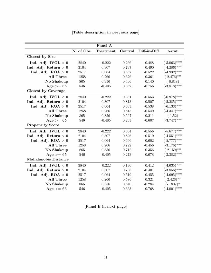
[Table description in previous page]

Panel A

N. of Obs. Treatment Control Diff-in-Diff t-stat

Closest by Size

Ind. Adj. IVOL < 0 2840 -0.222 0.266 -0.488 (-5.063)***Ind. Adj. Return > 0 2104 0.307 0.797 -0.490 (-4.286)***

Ind. Adj. ROA > 0 2517 0.064 0.587 -0.522 (-4.932)***All Three 1258 0.266 0.626 -0.361 (-2.476)**

No Shakeup 865 0.356 0.496 -0.140 (-0.818)Age >= 65 546 -0.405 0.352 -0.756 (-3.818)***

Closest by Coverage

Ind. Adj. IVOL < 0 2840 -0.222 0.331 -0.553 (-6.978)***Ind. Adj. Return > 0 2104 0.307 0.813 -0.507 (-5.285)***

Ind. Adj. ROA > 0 2517 0.064 0.603 -0.538 (-6.133)***All Three 1258 0.266 0.815 -0.549 (-4.347)***

No Shakeup 865 0.356 0.567 -0.211 (-1.52)Age >= 65 546 -0.405 0.203 -0.607 (-3.747)***

Propensity Score

Ind. Adj. IVOL < 0 2840 -0.222 0.334 -0.556 (-5.677)***Ind. Adj. Return > 0 2104 0.307 0.826 -0.519 (-4.551)***

Ind. Adj. ROA > 0 2517 0.064 0.666 -0.602 (-5.777)***All Three 1258 0.266 0.722 -0.456 (-3.176)***

No Shakeup 865 0.356 0.712 -0.356 (-2.159)**Age >= 65 546 -0.405 0.273 -0.678 (-3.382)***

Mahalanobis Distance

Ind. Adj. IVOL < 0 2840 -0.222 0.190 -0.412 (-4.635)***Ind. Adj. Return > 0 2104 0.307 0.708 -0.401 (-3.856)***

Ind. Adj. ROA > 0 2517 0.064 0.519 -0.455 (-4.695)***All Three 1258 0.266 0.586 -0.321 (-2.426)**

No Shakeup 865 0.356 0.640 -0.284 (-1.807)*Age >= 65 546 -0.405 0.363 -0.768 (-4.001)***

[Panel B in next page]

41

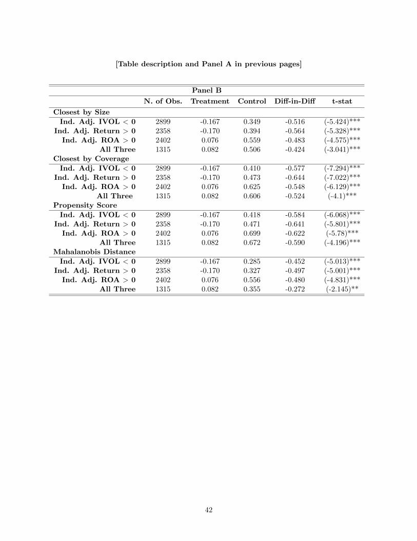
[Table description and Panel A in previous pages]

Panel B

N. of Obs. Treatment Control Diff-in-Diff t-stat

Closest by Size

Ind. Adj. IVOL < 0 2899 -0.167 0.349 -0.516 (-5.424)***Ind. Adj. Return > 0 2358 -0.170 0.394 -0.564 (-5.328)***

Ind. Adj. ROA > 0 2402 0.076 0.559 -0.483 (-4.575)***All Three 1315 0.082 0.506 -0.424 (-3.041)***

Closest by Coverage

Ind. Adj. IVOL < 0 2899 -0.167 0.410 -0.577 (-7.294)***Ind. Adj. Return > 0 2358 -0.170 0.473 -0.644 (-7.022)***

Ind. Adj. ROA > 0 2402 0.076 0.625 -0.548 (-6.129)***All Three 1315 0.082 0.606 -0.524 (-4.1)***

Propensity Score

Ind. Adj. IVOL < 0 2899 -0.167 0.418 -0.584 (-6.068)***Ind. Adj. Return > 0 2358 -0.170 0.471 -0.641 (-5.801)***

Ind. Adj. ROA > 0 2402 0.076 0.699 -0.622 (-5.78)***All Three 1315 0.082 0.672 -0.590 (-4.196)***

Mahalanobis Distance

Ind. Adj. IVOL < 0 2899 -0.167 0.285 -0.452 (-5.013)***Ind. Adj. Return > 0 2358 -0.170 0.327 -0.497 (-5.001)***

Ind. Adj. ROA > 0 2402 0.076 0.556 -0.480 (-4.831)***All Three 1315 0.082 0.355 -0.272 (-2.145)**

42

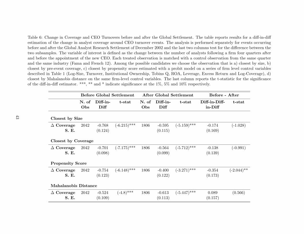
Table 6: Change in Coverage and CEO Turnovers before and after the Global Settlement. The table reports results for a diff-in-diffestimation of the change in analyst coverage around CEO turnover events. The analysis is performed separately for events occurringbefore and after the Global Analyst Research Settlement of December 2002 and the last two columns test for the difference between thetwo subsamples. The variable of interest is defined as the change between the number of analysts following a firm four quarters afterand before the appointment of the new CEO. Each treated observation is matched with a control observation from the same quarterand the same industry (Fama and French 12). Among the possible candidates we choose the observation that is a) closest by size, b)closest by pre-event coverage, c) closest by propensity score estimated with a probit model on a series of firm level control variablesdescribed in Table 1 (Log-Size, Turnover, Institutional Ownership, Tobins Q, ROA, Leverage, Excess Return and Log-Coverage), d)closest by Mahalanobis distance on the same firm-level control variables. The last column reports the t-statistic for the significanceof the diff-in-diff estimator. ***, ** and * indicate significance at the 1%, 5% and 10% respectively.

Before Global Settlement After Global Settlement Before - After

N. of Diff-in- t-stat N. of Diff-in- t-stat Diff-in-Diff- t-statObs Diff Obs Diff in-Diff

Closest by Size

∆ Coverage 2042 -0.768 (-6.215)*** 1806 -0.595 (-5.159)*** -0.174 (-1.028)S. E. (0.124) (0.115) (0.169)

Closest by Coverage

∆ Coverage 2042 -0.701 (-7.175)*** 1806 -0.564 (-5.712)*** -0.138 (-0.991)S. E. (0.098) (0.099) (0.139)

Propensity Score

∆ Coverage 2042 -0.754 (-6.148)*** 1806 -0.400 (-3.271)*** -0.354 (-2.044)**S. E. (0.123) (0.122) (0.173)

Mahalanobis Distance

∆ Coverage 2042 -0.524 (-4.8)*** 1806 -0.613 (-5.447)*** 0.089 (0.566)S. E. (0.109) (0.113) (0.157)

43

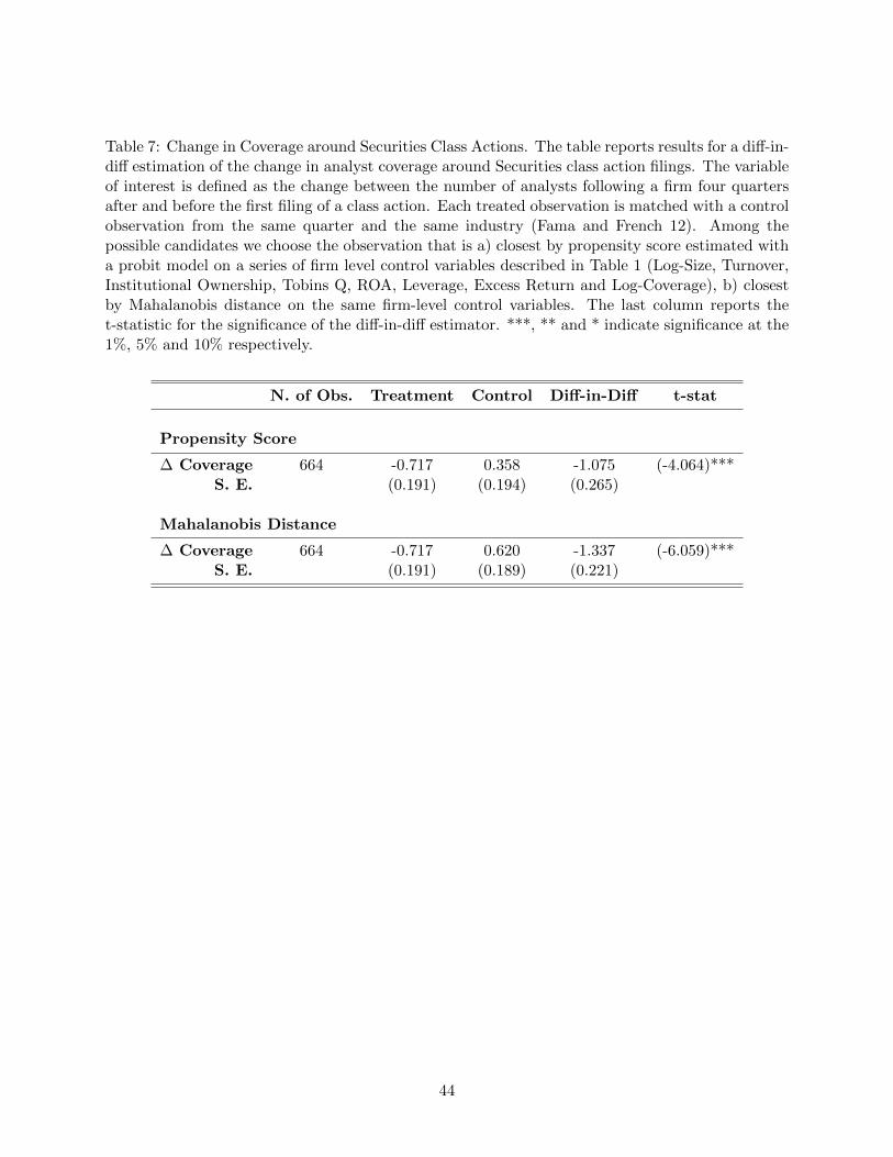
Table 7: Change in Coverage around Securities Class Actions. The table reports results for a diff-in-diff estimation of the change in analyst coverage around Securities class action filings. The variableof interest is defined as the change between the number of analysts following a firm four quartersafter and before the first filing of a class action. Each treated observation is matched with a controlobservation from the same quarter and the same industry (Fama and French 12). Among thepossible candidates we choose the observation that is a) closest by propensity score estimated witha probit model on a series of firm level control variables described in Table 1 (Log-Size, Turnover,Institutional Ownership, Tobins Q, ROA, Leverage, Excess Return and Log-Coverage), b) closestby Mahalanobis distance on the same firm-level control variables. The last column reports thet-statistic for the significance of the diff-in-diff estimator. ***, ** and * indicate significance at the1%, 5% and 10% respectively.

N. of Obs. Treatment Control Diff-in-Diff t-stat

Propensity Score

∆ Coverage 664 -0.717 0.358 -1.075 (-4.064)***S. E. (0.191) (0.194) (0.265)

Mahalanobis Distance

∆ Coverage 664 -0.717 0.620 -1.337 (-6.059)***S. E. (0.191) (0.189) (0.221)

44

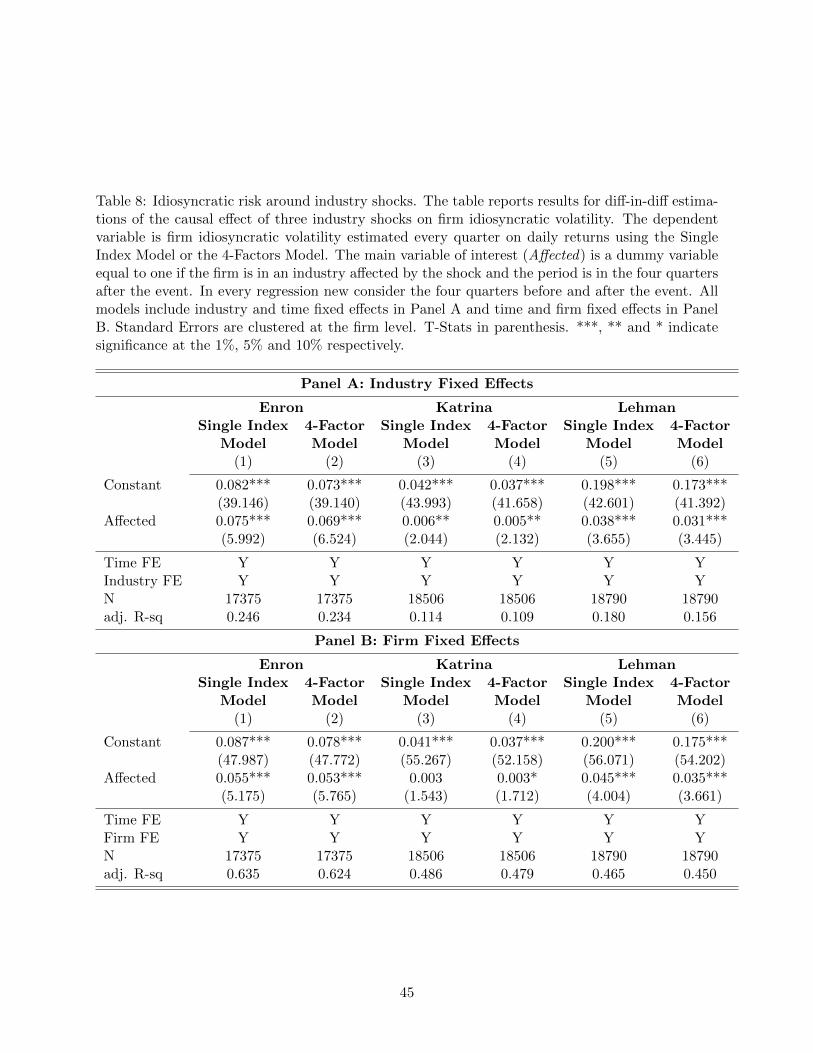
Table 8: Idiosyncratic risk around industry shocks. The table reports results for diff-in-diff estima-tions of the causal effect of three industry shocks on firm idiosyncratic volatility. The dependentvariable is firm idiosyncratic volatility estimated every quarter on daily returns using the SingleIndex Model or the 4-Factors Model. The main variable of interest (Affected) is a dummy variableequal to one if the firm is in an industry affected by the shock and the period is in the four quartersafter the event. In every regression new consider the four quarters before and after the event. Allmodels include industry and time fixed effects in Panel A and time and firm fixed effects in PanelB. Standard Errors are clustered at the firm level. T-Stats in parenthesis. ***, ** and * indicatesignificance at the 1%, 5% and 10% respectively.

Panel A: Industry Fixed Effects

Enron Katrina LehmanSingle Index 4-Factor Single Index 4-Factor Single Index 4-Factor

Model Model Model Model Model Model(1) (2) (3) (4) (5) (6)

Constant 0.082*** 0.073*** 0.042*** 0.037*** 0.198*** 0.173***(39.146) (39.140) (43.993) (41.658) (42.601) (41.392)

Affected 0.075*** 0.069*** 0.006** 0.005** 0.038*** 0.031***(5.992) (6.524) (2.044) (2.132) (3.655) (3.445)

Time FE Y Y Y Y Y YIndustry FE Y Y Y Y Y YN 17375 17375 18506 18506 18790 18790adj. R-sq 0.246 0.234 0.114 0.109 0.180 0.156

Panel B: Firm Fixed Effects

Enron Katrina LehmanSingle Index 4-Factor Single Index 4-Factor Single Index 4-Factor

Model Model Model Model Model Model(1) (2) (3) (4) (5) (6)

Constant 0.087*** 0.078*** 0.041*** 0.037*** 0.200*** 0.175***(47.987) (47.772) (55.267) (52.158) (56.071) (54.202)

Affected 0.055*** 0.053*** 0.003 0.003* 0.045*** 0.035***(5.175) (5.765) (1.543) (1.712) (4.004) (3.661)

Time FE Y Y Y Y Y YFirm FE Y Y Y Y Y YN 17375 17375 18506 18506 18790 18790adj. R-sq 0.635 0.624 0.486 0.479 0.465 0.450

45

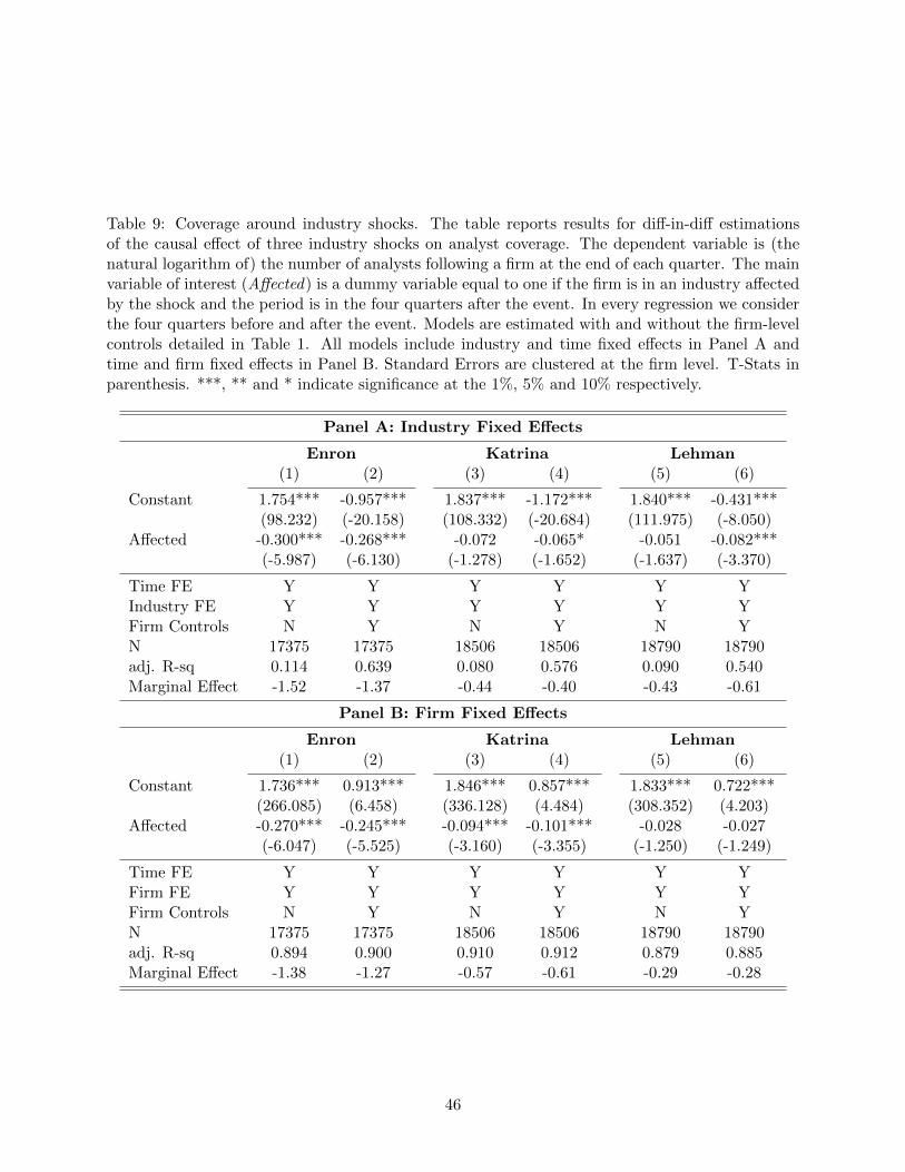
Table 9: Coverage around industry shocks. The table reports results for diff-in-diff estimationsof the causal effect of three industry shocks on analyst coverage. The dependent variable is (thenatural logarithm of) the number of analysts following a firm at the end of each quarter. The mainvariable of interest (Affected) is a dummy variable equal to one if the firm is in an industry affectedby the shock and the period is in the four quarters after the event. In every regression we considerthe four quarters before and after the event. Models are estimated with and without the firm-levelcontrols detailed in Table 1. All models include industry and time fixed effects in Panel A andtime and firm fixed effects in Panel B. Standard Errors are clustered at the firm level. T-Stats inparenthesis. ***, ** and * indicate significance at the 1%, 5% and 10% respectively.

Panel A: Industry Fixed Effects

Enron Katrina Lehman(1) (2) (3) (4) (5) (6)

Constant 1.754*** -0.957*** 1.837*** -1.172*** 1.840*** -0.431***(98.232) (-20.158) (108.332) (-20.684) (111.975) (-8.050)

Affected -0.300*** -0.268*** -0.072 -0.065* -0.051 -0.082***(-5.987) (-6.130) (-1.278) (-1.652) (-1.637) (-3.370)

Time FE Y Y Y Y Y YIndustry FE Y Y Y Y Y YFirm Controls N Y N Y N YN 17375 17375 18506 18506 18790 18790adj. R-sq 0.114 0.639 0.080 0.576 0.090 0.540Marginal Effect -1.52 -1.37 -0.44 -0.40 -0.43 -0.61

Panel B: Firm Fixed Effects

Enron Katrina Lehman(1) (2) (3) (4) (5) (6)

Constant 1.736*** 0.913*** 1.846*** 0.857*** 1.833*** 0.722***(266.085) (6.458) (336.128) (4.484) (308.352) (4.203)

Affected -0.270*** -0.245*** -0.094*** -0.101*** -0.028 -0.027(-6.047) (-5.525) (-3.160) (-3.355) (-1.250) (-1.249)

Time FE Y Y Y Y Y YFirm FE Y Y Y Y Y YFirm Controls N Y N Y N YN 17375 17375 18506 18506 18790 18790adj. R-sq 0.894 0.900 0.910 0.912 0.879 0.885Marginal Effect -1.38 -1.27 -0.57 -0.61 -0.29 -0.28

46

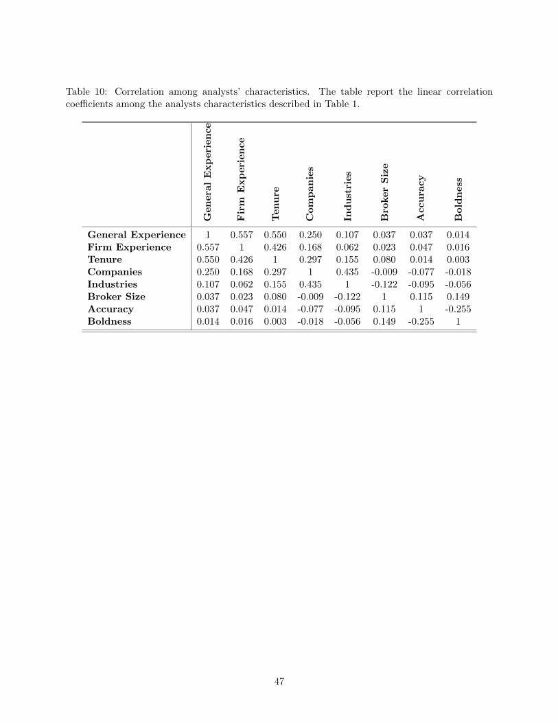
Table 10: Correlation among analysts’ characteristics. The table report the linear correlationcoefficients among the analysts characteristics described in Table 1.

Gen

era

lE

xp

eri

en

ce

Fir

mE

xp

eri

en

ce

Tenu

re

Com

pan

ies

Ind

ust

ries

Bro

ker

Siz

e

Accu

racy

Bold

ness

General Experience 1 0.557 0.550 0.250 0.107 0.037 0.037 0.014Firm Experience 0.557 1 0.426 0.168 0.062 0.023 0.047 0.016Tenure 0.550 0.426 1 0.297 0.155 0.080 0.014 0.003Companies 0.250 0.168 0.297 1 0.435 -0.009 -0.077 -0.018Industries 0.107 0.062 0.155 0.435 1 -0.122 -0.095 -0.056Broker Size 0.037 0.023 0.080 -0.009 -0.122 1 0.115 0.149Accuracy 0.037 0.047 0.014 -0.077 -0.095 0.115 1 -0.255Boldness 0.014 0.016 0.003 -0.018 -0.056 0.149 -0.255 1

47

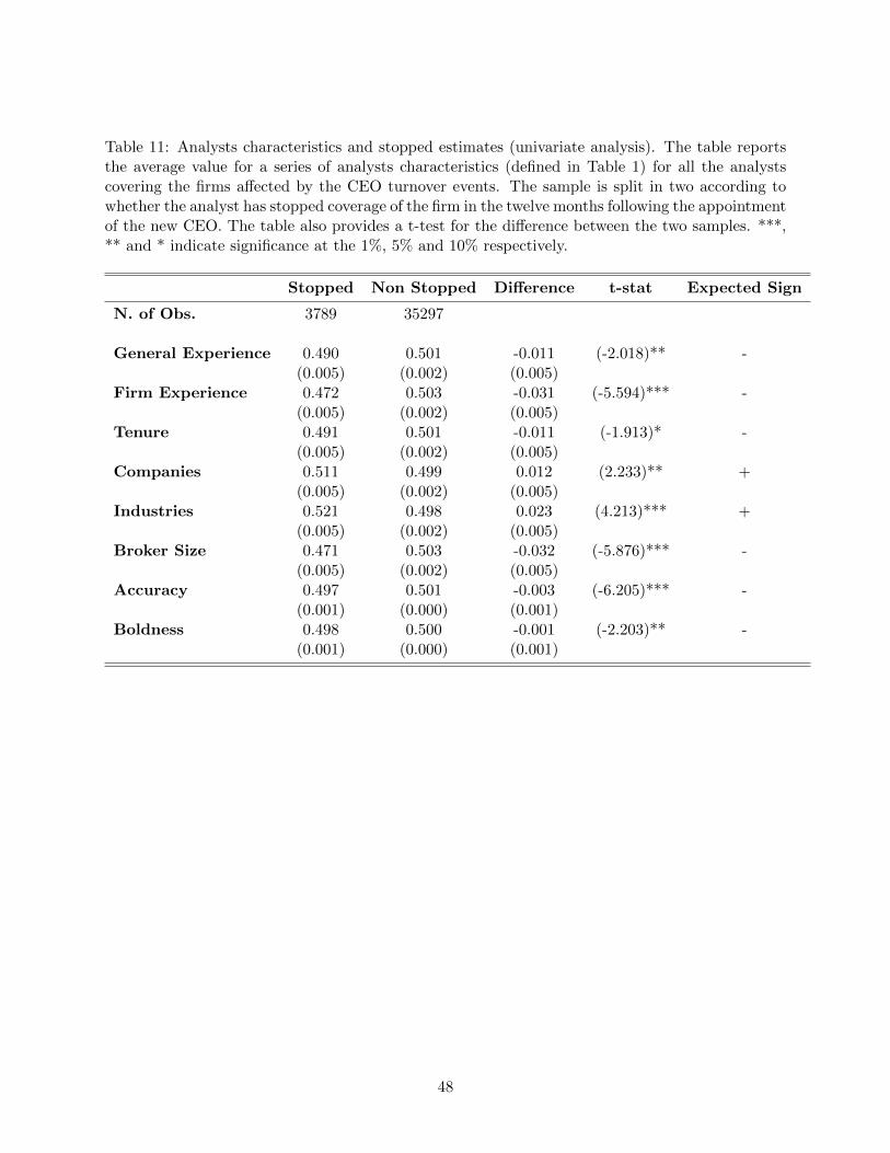
Table 11: Analysts characteristics and stopped estimates (univariate analysis). The table reportsthe average value for a series of analysts characteristics (defined in Table 1) for all the analystscovering the firms affected by the CEO turnover events. The sample is split in two according towhether the analyst has stopped coverage of the firm in the twelve months following the appointmentof the new CEO. The table also provides a t-test for the difference between the two samples. ***,** and * indicate significance at the 1%, 5% and 10% respectively.

Stopped Non Stopped Difference t-stat Expected Sign

N. of Obs. 3789 35297

General Experience 0.490 0.501 -0.011 (-2.018)** -(0.005) (0.002) (0.005)

Firm Experience 0.472 0.503 -0.031 (-5.594)*** -(0.005) (0.002) (0.005)

Tenure 0.491 0.501 -0.011 (-1.913)* -(0.005) (0.002) (0.005)

Companies 0.511 0.499 0.012 (2.233)** +(0.005) (0.002) (0.005)

Industries 0.521 0.498 0.023 (4.213)*** +(0.005) (0.002) (0.005)

Broker Size 0.471 0.503 -0.032 (-5.876)*** -(0.005) (0.002) (0.005)

Accuracy 0.497 0.501 -0.003 (-6.205)*** -(0.001) (0.000) (0.001)

Boldness 0.498 0.500 -0.001 (-2.203)** -(0.001) (0.000) (0.001)

48

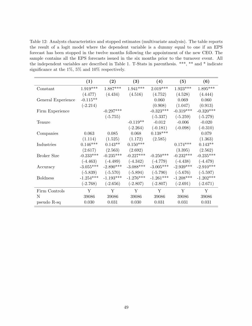
Table 12: Analysts characteristics and stopped estimates (multivariate analysis). The table reportsthe result of a logit model where the dependent variable is a dummy equal to one if an EPSforecast has been stopped in the twelve months following the appointment of the new CEO. Thesample contains all the EPS forecasts issued in the six months prior to the turnover event. Allthe independent variables are described in Table 1. T-Stats in parenthesis. ***, ** and * indicatesignificance at the 1%, 5% and 10% respectively.

(1) (2) (3) (4) (5) (6)

Constant 1.919*** 1.887*** 1.941*** 2.019*** 1.923*** 1.895***(4.477) (4.434) (4.516) (4.752) (4.528) (4.444)

General Experience -0.115** 0.060 0.069 0.060(-2.214) (0.908) (1.047) (0.913)

Firm Experience -0.297*** -0.323*** -0.319*** -0.320***(-5.755) (-5.337) (-5.259) (-5.279)

Tenure -0.119** -0.012 -0.006 -0.020(-2.264) (-0.181) (-0.098) (-0.310)

Companies 0.063 0.085 0.068 0.138*** 0.079(1.114) (1.525) (1.172) (2.585) (1.363)

Industries 0.146*** 0.143** 0.150*** 0.174*** 0.143**(2.617) (2.563) (2.692) (3.395) (2.562)

Broker Size -0.233*** -0.235*** -0.227*** -0.250*** -0.232*** -0.235***(-4.463) (-4.489) (-4.342) (-4.779) (-4.438) (-4.479)

Accuracy -3.055*** -2.890*** -3.088*** -3.005*** -2.939*** -2.910***(-5.839) (-5.570) (-5.894) (-5.790) (-5.676) (-5.597)

Boldness -1.254*** -1.193*** -1.276*** -1.261*** -1.208*** -1.202***(-2.768) (-2.656) (-2.807) (-2.807) (-2.691) (-2.671)

Firm Controls Y Y Y Y Y YN 39086 39086 39086 39086 39086 39086pseudo R-sq 0.030 0.031 0.030 0.031 0.031 0.031

49

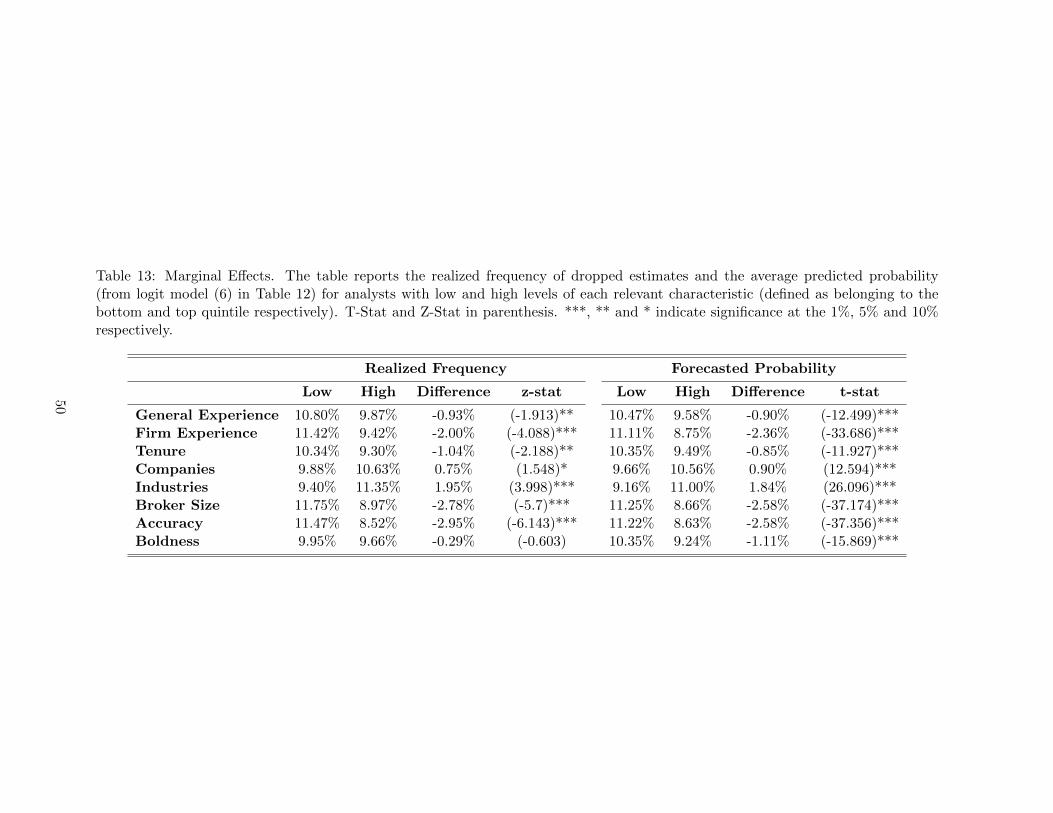
Table 13: Marginal Effects. The table reports the realized frequency of dropped estimates and the average predicted probability(from logit model (6) in Table 12) for analysts with low and high levels of each relevant characteristic (defined as belonging to thebottom and top quintile respectively). T-Stat and Z-Stat in parenthesis. ***, ** and * indicate significance at the 1%, 5% and 10%respectively.

Realized Frequency Forecasted Probability

Low High Difference z-stat Low High Difference t-stat

General Experience 10.80% 9.87% -0.93% (-1.913)** 10.47% 9.58% -0.90% (-12.499)***Firm Experience 11.42% 9.42% -2.00% (-4.088)*** 11.11% 8.75% -2.36% (-33.686)***Tenure 10.34% 9.30% -1.04% (-2.188)** 10.35% 9.49% -0.85% (-11.927)***Companies 9.88% 10.63% 0.75% (1.548)* 9.66% 10.56% 0.90% (12.594)***Industries 9.40% 11.35% 1.95% (3.998)*** 9.16% 11.00% 1.84% (26.096)***Broker Size 11.75% 8.97% -2.78% (-5.7)*** 11.25% 8.66% -2.58% (-37.174)***Accuracy 11.47% 8.52% -2.95% (-6.143)*** 11.22% 8.63% -2.58% (-37.356)***Boldness 9.95% 9.66% -0.29% (-0.603) 10.35% 9.24% -1.11% (-15.869)***

50

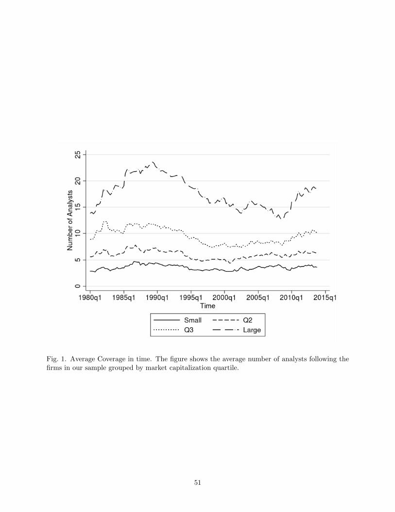
Fig. 1. Average Coverage in time. The figure shows the average number of analysts following thefirms in our sample grouped by market capitalization quartile.

51

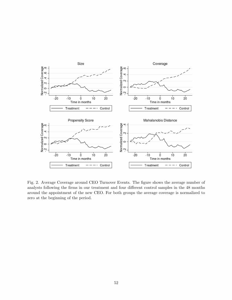
Fig. 2. Average Coverage around CEO Turnover Events. The figure shows the average number ofanalysts following the firms in our treatment and four different control samples in the 48 monthsaround the appointment of the new CEO. For both groups the average coverage is normalized tozero at the beginning of the period.

52

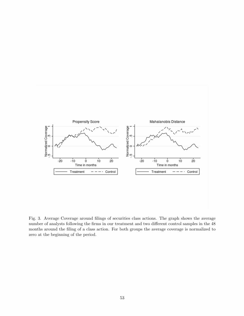
Fig. 3. Average Coverage around filings of securities class actions. The graph shows the averagenumber of analysts following the firms in our treatment and two different control samples in the 48months around the filing of a class action. For both groups the average coverage is normalized tozero at the beginning of the period.

53