Embed Size (px)
Citation preview

Unclassified NEA/CSNI/R(2015)19 Organisation de Coopération et de Développement Économiques Organisation for Economic Co-operation and Development 08-Jan-2016
___________________________________________________________________________________________
_____________ English - Or. English NUCLEAR ENERGY AGENCY
COMMITTEE ON THE SAFETY OF NUCLEAR INSTALLATIONS
Benchmarking of Fast-Running Software Tools Used to Model Releases During Nuclear Accidents
JT03388769
Complete document available on OLIS in its original format
This document and any map included herein are without prejudice to the status of or sovereignty over any territory, to the delimitation of
international frontiers and boundaries and to the name of any territory, city or area.
NE
A/C
SN
I/R(2
01
5)1
9
Un
classified
En
glish
- Or. E
ng
lish
NEA/CSNI/R(2015)19
2
ORGANISATION FOR ECONOMIC CO-OPERATION AND DEVELOPMENT
The OECD is a unique forum where the governments of 34 democracies work together to address the economic, social and
environmental challenges of globalisation. The OECD is also at the forefront of efforts to understand and to help governments
respond to new developments and concerns, such as corporate governance, the information economy and the challenges of an
ageing population. The Organisation provides a setting where governments can compare policy experiences, seek answers to
common problems, identify good practice and work to co-ordinate domestic and international policies.
The OECD member countries are: Australia, Austria, Belgium, Canada, Chile, the Czech Republic, Denmark, Estonia,
Finland, France, Germany, Greece, Hungary, Iceland, Ireland, Israel, Italy, Japan, Luxembourg, Mexico, the Netherlands, New
Zealand, Norway, Poland, Portugal, the Republic of Korea, the Slovak Republic, Slovenia, Spain, Sweden, Switzerland,
Turkey, the United Kingdom and the United States. The European Commission takes part in the work of the OECD.
OECD Publishing disseminates widely the results of the Organisation’s statistics gathering and research on economic,
social and environmental issues, as well as the conventions, guidelines and standards agreed by its members.
NUCLEAR ENERGY AGENCY
The OECD Nuclear Energy Agency (NEA) was established on 1 February 1958. Current NEA membership consists of
31 countries: Australia, Austria, Belgium, Canada, the Czech Republic, Denmark, Finland, France, Germany, Greece, Hungary,
Iceland, Ireland, Italy, Japan, Luxembourg, Mexico, the Netherlands, Norway, Poland, Portugal, the Republic of Korea, the
Russian Federation, the Slovak Republic, Slovenia, Spain, Sweden, Switzerland, Turkey, the United Kingdom and the United
States. The European Commission also takes part in the work of the Agency.
The mission of the NEA is:
– to assist its member countries in maintaining and further developing, through international co-operation, the scientific,
technological and legal bases required for a safe, environmentally friendly and economical use of nuclear energy for
peaceful purposes;
– to provide authoritative assessments and to forge common understandings on key issues, as input to government
decisions on nuclear energy policy and to broader OECD policy analyses in areas such as energy and sustainable
development.
Specific areas of competence of the NEA include the safety and regulation of nuclear activities, radioactive waste
management, radiological protection, nuclear science, economic and technical analyses of the nuclear fuel cycle, nuclear law
and liability, and public information.
The NEA Data Bank provides nuclear data and computer program services for participating countries. In these and related
tasks, the NEA works in close collaboration with the International Atomic Energy Agency in Vienna, with which it has a Co-
operation Agreement, as well as with other international organisations in the nuclear field.
This document and any map included herein are without prejudice to the status of or sovereignty over any territory, to the delimitation of international
frontiers and boundaries and to the name of any territory, city or area.
Corrigenda to OECD publications may be found online at: www.oecd.org/publishing/corrigenda.
© OECD 2015
You can copy, download or print OECD content for your own use, and you can include excerpts from OECD publications, databases and multimedia products
in your own documents, presentations, blogs, websites and teaching materials, provided that suitable acknowledgment of the OECD as source and copyright
owner is given. All requests for public or commercial use and translation rights should be submitted to [email protected]. Requests for permission to photocopy portions of this material for public or commercial use shall be addressed directly to the Copyright Clearance Center (CCC) at [email protected]
or the Centre français d'exploitation du droit de copie (CFC) [email protected].

NEA/CSNI/R(2015)19
3
COMMITTEE ON THE SAFETY OF NUCLEAR INSTALLATIONS
The NEA Committee on the Safety of Nuclear Installations (CSNI) is an international committee made up
of senior scientists and engineers with broad responsibilities for safety technology and research
programmes, as well as representatives from regulatory authorities. It was created in 1973 to develop and
co-ordinate the activities of the NEA concerning the technical aspects of the design, construction and
operation of nuclear installations insofar as they affect the safety of such installations.
The committee’s purpose is to foster international co-operation in nuclear safety among NEA member
countries. The main tasks of the CSNI are to exchange technical information and to promote collaboration
between research, development, engineering and regulatory organisations; to review operating experience
and the state of knowledge on selected topics of nuclear safety technology and safety assessment; to
initiate and conduct programmes to overcome discrepancies, develop improvements and reach consensus
on technical issues; and to promote the co-ordination of work that serves to maintain competence in
nuclear safety matters, including the establishment of joint undertakings.
The priority of the CSNI is on the safety of nuclear installations and the design and construction of
new reactors and installations. For advanced reactor designs, the committee provides a forum for
improving safety-related knowledge and a vehicle for joint research.
In implementing its programme, the CSNI establishes co-operative mechanisms with the
NEA Committee on Nuclear Regulatory Activities (CNRA), which is responsible for issues concerning the
regulation, licensing and inspection of nuclear installations with regard to safety. It also co-operates with
other NEA Standing Technical Committees, as well as with key international organisations such as the
International Atomic Energy Agency (IAEA), on matters of common interest.

NEA/CSNI/R(2015)19
4

NEA/CSNI/R(2015)19
5
TABLE OF CONTENTS
EXECUTIVE SUMMARY ............................................................................................................................. 7
LIST OF ACRONYMS ................................................................................................................................. 11
1 INTRODUCTION ..................................................................................................................................... 13
1.1 Background .......................................................................................................................................... 13 1.2 Objective .............................................................................................................................................. 13 1.3 Scope .................................................................................................................................................... 14 1.4 Methodology ........................................................................................................................................ 15 1.5 Structure of the Report ......................................................................................................................... 16
2 OVERVIEW OF TOOLS ........................................................................................................................... 17
2.1 Primary Uses of the Software Tools .................................................................................................... 19 2.2 Modelling Capabilities ......................................................................................................................... 19 2.3 Source Term Algorithms ...................................................................................................................... 21 2.4 Dispersion Models ............................................................................................................................... 25 2.5 Running the Software .......................................................................................................................... 26 2.6 Software Output ................................................................................................................................... 31 2.7 Validation ............................................................................................................................................. 35 2.8 Summary .............................................................................................................................................. 37
3 DESCRIPTION OF MODELLED SCENARIOS ...................................................................................... 49
3.1 Peach Bottom ....................................................................................................................................... 50 3.2 Surry ..................................................................................................................................................... 53 3.3 Oskarshamn ......................................................................................................................................... 56 3.4 Golfech ................................................................................................................................................. 58 3.5 Point Lepreau ....................................................................................................................................... 61
4 RESULTS OF PEACH BOTTOM SIMULATION USING FAST-RUNNING TOOLS ......................... 65
4.1 Assumptions in Modelling the Peach Bottom Scenario ....................................................................... 65 4.2 Peach Bottom Results .......................................................................................................................... 68
5 RESULTS OF SURRY SIMULATION USING FAST-RUNNING TOOLS ........................................... 75
5.1 Assumptions in Modelling the Surry Scenario .................................................................................... 75 5.2 Surry Results ........................................................................................................................................ 78
6 RESULTS OF OSKARSHAMN SIMULATION USING FAST RUNNING TOOLS ............................. 87
6.1 Assumptions in Modelling the Oskarshamn Scenario ......................................................................... 87 6.2 Oskarshamn Results ............................................................................................................................. 90
7 RESULTS OF GOLFECH SIMULATION USING FAST-RUNNING TOOLS ...................................... 95
7.1 Assumptions in Modelling the Golfech Scenario ................................................................................ 95

NEA/CSNI/R(2015)19
6
7.2 Golfech Results .................................................................................................................................... 97
8 RESULTS OF POINT LEPREAU SIMULATION USING FAST-RUNNING TOOLS ........................ 105
8.1 Assumptions in Modelling the Point Lepreau Scenario ..................................................................... 105 8.2 Point Lepreau Results ........................................................................................................................ 106
9 ASSESSMENT OF RESULTS ................................................................................................................ 113
9.1 Source Term ....................................................................................................................................... 113 9.2 Factors Affecting Source Term Calculations ..................................................................................... 120 9.3 Doses .................................................................................................................................................. 128 9.4 Factors Affecting Dose Calculations ................................................................................................. 132
10 SUMMARY AND RECOMMENDATIONS ........................................................................................ 137
10.1 Benchmarking highlights ................................................................................................................. 137 10.2 Future efforts .................................................................................................................................... 139
11. REFERENCES ...................................................................................................................................... 142

NEA/CSNI/R(2015)19
7
EXECUTIVE SUMMARY
The accident at the Fukushima nuclear power plant highlighted the importance of effective nuclear
accident response, including reliable estimation of potential consequences and implementing actions as
appropriate in response to the anticipated consequences. However, the complexity of the accident,
combined with the wide-spread effects of the earthquake and tsunami, greatly impacted the ability to
provide timely and accurate information to national and international stakeholders. It was also observed
that the recommendations for protection measures given by different foreign governments to their citizens
occasionally differed, especially at the initial stages of the accident. Such differences may be attributed to
several factors, including the methods that were used to assess accident progression and develop
reasonable estimates of radionuclide releases to the environment. These differences can, in turn, affect the
projected radiological dose to a member of the public.
A tri-committee CNRA-CRPPH-CSNI group recommended that “CSNI should analyse the
comparison of source-term methodologies utilised by countries and determine if or why the dose prediction
differed for Fukushima.” Therefore, a comparison of methodologies was undertaken and is presented in
this report. More specifically, this summary report provides the following information:
A list of the software tools for assessing the source term and public doses as well as a brief description
of their features
An overview of the current capabilities of the existing software tools, determined based on
participants’ responses to a questionnaire
A summary of hypothetical accident scenarios that were used to develop source terms and dose
projections for comparing software tool capabilities
An assessment of the results from modelling the hypothetical accident scenarios, including factors that
can influence software tools outputs.
The objective of this joint WGAMA-WPNEM activity was to benchmark software tools used to
estimate consequences of accidents at nuclear facilities. Two aspects of accident consequences were
considered: amounts of radioactive material releases as well as public doses resulting from such releases.
This activity and the recommended follow-up steps are expected to promote better understanding of the
existing predictive capability currently available in a number of organisations to rapidly assess and
recommend protective measures during nuclear emergencies. Several recommendations are provided to
direct future efforts in this area. The final deliverable of the activity was set to be a report summarising the
benchmark study.
Software tools evaluated in this benchmarking study demonstrated the ability to:
Calculate fission-product source terms and provide an estimate of core damage state and the condition
of the physical barrier;
Project radiological doses from fission product releases during initial accident stages;
Execute with a small number of input parameters (at the start of a nuclear accident only limited
information will be available for use);

NEA/CSNI/R(2015)19
8
Incorporate additional details as more information becomes available and improve the predicted
results;
Model fission-product releases from different reactor technologies;
Complete calculations rapidly in support of protective-action decision-making;
Predict source terms and radiological doses accurately;
Produce results in a clear, user-friendly and logical manner for use in making protective action
recommendations.
The first step in the project was to identify software tools to be included in the benchmarking study.
This was accomplished by requesting participating organisations to identify software that is currently used
to model fission product releases from nuclear facilities during emergencies. Questionnaires were
developed early in the study to gather information on how the tools work, what they are used for, and to
identify potential strengths and weaknesses. The questionnaires were provided to participating
organisations to collect a relatively complete dataset that characterises the tools.
Twenty organisations, representing twelve countries and two international organisations, participated
in this benchmarking project. Between them, a total of twenty-five software tools were included in this
exercise and used to assess the source term and/or dose consequences of one to five hypothetical accident
scenarios.
The second step in the project was to select a set of appropriate hypothetical scenarios for the
software tools to model. The scenarios were developed to represent several types of nuclear reactors: a
pressurised water reactor (PWR), boiling water reactor (BWR), and Canada deuterium uranium (CANDU)
reactors. The amount of data provided initially was purposely limited so participants would perform blind
simulations.
It is important to note that the accident scenarios used in this benchmarking exercise are
hypothetical. They were deliberately selected to represent relatively extreme cases, regardless of the fact
that they would be extremely unlikely.
Five different hypothetical accident scenarios were developed and used in the benchmarking
modelling, which are as follows:
An unmitigated, long-term station blackout at Peach Bottom Unit 3, an American BWR;
An unmitigated, long-term station blackout at Surry Unit 1, an American PWR;
A transient resulting in a loss of residual heat removal at Oskarshamn Unit3, a Swedish BWR;
A large break LOCA with failure of safety functions at Golfech Unit 1, a French PWR;
A station blackout with emergency power generators at Point Lepreau, a Canadian PHWR.
Three different datasets were presented for each scenario, each with increasing amounts of data, to
allow evaluations of how well the software coped with limited information on the accident scenario. These
datasets were intended to represent different depths of information typically available to emergency
response organisations during accident progression. The three datasets are as follows:
1 hour into the accident scenario, when only the reactor location and initiating event are known;
6 hours into the accident scenario, when data on core cooling is available along with additional
information on the accident scenario;
24 hours into the accident scenario, when the status of containment and other key information is
known.

NEA/CSNI/R(2015)19
9
Participants were provided meteorological data for each accident location for modelling of plume
dispersion. Meteorological data was chosen to be representative of actual weather conditions near the
reactor sites on specific dates.
The third and the most important step in the study was to use the software tools in simulations of
the selected scenarios. The participating organisations used their software tools to run the three dataset for
as many of the scenarios/reactor types as possible.
This study showed that the software tools will likely provide different source term and dose estimates
when used with limited information for the same accident scenario. Reasons for these differences are
identified and discussed in this report. Important factors are the models incorporated in the software and
the assumptions made by participants when selecting input parameters to model accident progression. The
assumptions made with limited data had a major effect on source term prediction. For example, some
participants assumed that a significant release was inevitable and selected input parameters accordingly,
whereas some participants did not assume a significant release unless stated in the dataset (only the 24-
hour dataset indicated a significant release). The importance of assumptions regarding accident progression
is illustrated by differences in source terms estimated by two different organisations using the same
software for the same scenario.
Other factors affecting source term prediction include:
Assumptions on initial core inventory;
Definition of the pathway to the environment;
Code capability to model certain systems;
Assumptions related to the containment failure;
Modelling of chemical species of iodine;
Knowledge of different reactor designs;
Ability to model different reactor designs.
Potential reasons why predicted doses varied were also considered, but their effects could not be
conclusively determined within the scope of this study. Possible causes of variations amongst dose
predictions can be attributed to differences in the following:
Source terms, including the timing and duration of atmospheric releases;
Site definition, including how the terrain and surface roughness was defined;
Atmospheric dispersion, including the assumptions used to process the weather data provided for
this study;
Dose calculation models;
Dose conversion factors.
Some participants who responded to the questionnaire were unable to provide results for all of the
analyses needed for this study. Several reasons are attributed to this limitation:
Software could not model the scenario for a specific reactor type;
Software is under development;
Greater than expected time required to perform the requested analyses.
A consideration for follow-on work to this study is a more comprehensive analysis of the reasons for
differences in source term and dose results using fast-running software for emergency response. Further
study of source term, atmospheric transport, and dose calculation models in these software tools would

NEA/CSNI/R(2015)19
10
benefit decision-making for formulating protective action recommendations. Also, strategies for quickly
predicting accident progression and projecting consequences could be a useful undertaking. In addition, a
forum for exchange of best practices and training for users of the software should be considered.
The outcomes of the present study should be useful for understanding existing software capabilities
for rapid estimation of accident source terms and doses to members of the public, in view of their current
limitations and use by practitioners in the field.

NEA/CSNI/R(2015)19
11
LIST OF ACRONYMS
Note that the list of acronyms does not include the names of the software tools (as not all of them are
acronyms). Also not included are units and chemical element symbols.
AECL – Atomic Energy of Canada Limited
BBN – Bayesian belief network
BWR – boiling-water reactor
CANDU – Canadian deuterium uranium
CCI – core-concrete interaction
CHRS – containment heat removal system
CNRA – Committee on Nuclear Regulatory Activities (a committee of OECD-NEA)
CNSC – Canadian Nuclear Safety Commission
CRPPH - Committee on Radiation Protection and Public Health (a committee of OECD-NEA)
CSNI – Committee on the Safety of Nuclear Installations (a committee of OECD-NEA)
DEMA – Danish Emergency Management Agency
ECCS – emergency core cooling system
ENEA – Agenzia nazionale per le nuove tecnologie, l’energia e lo sviluppo economico sostenible (Italy)
EOC – emergency operations centre
GRS – Gesellschaft für Anlagen- und Reaktorsicherheit (Germany)
HC – Health Canada
IAEA – International Atomic Energy Agency
ICRP - International Commission on Radiological Protection
IRSN – Institut de Radioprotection et de Sûreté Nucléaire (France)
ISLOCA – interfacing-system loss-of-coolant accident
JRC – Joint Research Centre (part of European Commission)
KAERI – Korea Atomic Energy Research Institute
KI – potassium iodide
KIT – Karlsruhe Institute of Technology
LOCA – loss-of-coolant accident
LWR – light-water reactor
MVSS – multi-Venturi scrubbing system
NCBJ – National Centre for Nuclear Research (Poland)
NEA – Nuclear Energy Agency
NPCIL – Nuclear Power Corporation of India Limited
NPP – nuclear power plant
OECD – Organisation for Economic Co-operation and Development
OPEX – operating experience
PHWR – pressurised heavy-water reactor
PORV – power operated relief valve
PSA – probabilistic safety assessment
PWR – pressurised-water reactor
RAM – random access memory

NEA/CSNI/R(2015)19
12
RCIC – reactor core isolation cooling
RHR – residual heat removal
RPV – reactor pressure vessel
SBGTS – stand-by gas treatment system
SGTR – steam generator tube rupture
SOARCA – State-of-the-Art Reactor Consequence Analyses
SRV – safety relief valve
SSM – Swedish Radiation Safety Authority
ST – source term
TD-AFW – turbine driven auxiliary feed-water
TEDE – total effective dose equivalent
USNRC – United States Nuclear Regulatory Commission
WGAMA – Working Group on the Analysis and Management of Accidents (part of CSNI)
WPNEM – Working Party on Nuclear Emergency Matters (part of CRPPH)

NEA/CSNI/R(2015)19
13
1 INTRODUCTION
1.1 Background
The accident at the Fukushima nuclear power plant highlighted the importance of effective nuclear
accident response, including reliable estimation of potential consequences and implementing actions as
appropriate in response to the anticipated consequences. However, the complexity of the accident,
combined with the wide-spread effects of the earthquake and tsunami, greatly impacted the ability to
provide timely and accurate information to national and international stakeholders. It was also observed
that the recommendations for protection measures given by different foreign governments to their citizens
occasionally differed, especially at the initial stages of the accident. Such differences may be attributed to
several factors, including the methods that were used to assess accident progression and develop
reasonable estimates of radionuclide releases to the environment. These differences can, in turn, affect the
projected radiological dose to a member of the public.
As stated in the NEA report “The Fukushima Daiichi Nuclear Power Plant Accident: OECD/NEA
Nuclear Safety Response and Lessons Learnt”, an accident can never be completely ruled out. Because of
that, the necessary provisions for managing a radiological emergency situation at onsite and offsite
locations must be planned, tested and regularly reviewed in order to integrate lessons learned from drills
and from the management of actual incidents. In accordance with this directive, the CNRA Senior-level
Task Group on Impacts of the Fukushima Daiichi NPP Accident (STG-FUKU) recommended that “the
CSNI should analyse the comparison of source term methodologies utilised by countries and determine if
or why the dose prediction differed for Fukushima.” The first part of this recommendation – that related to
a comparison of methodologies – was undertaken and is presented in this report. More specifically, this
report provides the following information:
A list of existing software tools for assessing the source term and public doses as well as a brief
description of their features;
An overview of the current capabilities of existing software tools, based on participants’ responses to a
questionnaire;
A summary of hypothetical accident scenarios that were used to develop source terms and dose
projections for comparing software tool capabilities;
An assessment of the results from modelling the hypothetical accident scenarios, including factors that
can influence software tools outputs.
1.2 Objective
The objective of this joint WGAMA/WPNEM activity was to benchmark software tools used to
estimate consequences of accidents at nuclear facilities. Two aspects of accident consequences were
considered: amounts of radioactive material releases inside and outside the containment boundary as well
as public doses resulting from such releases. The benchmarking was intended to help identify strengths and
weaknesses of the tools used for source term and dispersion modelling. This activity and the recommended
follow-up steps are expected to promote better understanding of the existing predictive capabilities in a

NEA/CSNI/R(2015)19
14
number of organisations for rapidly assessing and recommending protective measures during nuclear
emergencies.
The final deliverable of the activity was set to be a state-of-the-art report summarising the benchmark
study. This report covers the software examined, scenarios used for benchmarking, results of benchmark
exercises, overview of capabilities of the software tools and areas for improvement.
This report can also serve as a database documenting the various fast-running reactor accident
software programmes used for emergency response and their advantages and disadvantages. This includes
comparisons of the various software tools and their ability to simulate accident scenarios, estimate source
terms, to predict doses, as well as their versatility (i.e., the ability to model different types of facilities),
accuracy and speed of calculation. Recommendations by the project team are based upon the findings of
the benchmarking and can be used to inform the future work on development of predictive capabilities for
accidents at nuclear facilities.
The results of this benchmarking could be of use to code developers, allowing them to identify areas
for improving existing software tools. The results could also benefit international organisations, operators,
research institutes, nuclear regulators and emergency management organisations by providing information
for allows comparison of options for assessing a nuclear emergency and determining which one best suits
their needs for response. In addition, the results provide interested organisations with an understanding of
hypothetical accident scenarios and interpretations as performed by organisations participating in the
benchmark study in the state-of-the-art report. Such an understanding of different modelling abilities and
techniques allows better insights on accident progressions and possible outcomes.
1.3 Scope
The focus of this benchmarking activity is on fast-running software tools that may be used while a
nuclear accident is in progress. These software tools usually have the capabilities to calculate:
a time-dependent “source term1” for the atmospheric release of radioactive materials,
on-site and off-site atmospheric transport, dispersion and deposition of the source term, and
dose projections from cloud shine, ground shine, and inhalation pathways as a function of location.
The primary use of these fast running software tools is to assist organisations with making rapid dose
assessments during a nuclear emergency. This benchmarking effort did not include more comprehensive
analytic codes, such as ASTEC and MELCOR, which are not intended for emergency response
applications. Such computer codes may not be suitable for use during emergencies due to run time
requirements and time required to setup input files. While operators of a facility undergoing an accident
may have such tools available; other organisations and countries involved in emergency response may rely
on fast-running software tools for making rapid dose projections assessment and protective action
recommendations.
The software tools were selected for participation in this benchmarking based on their ability to meet
the following criteria:
Calculate the fission product source terms and provide an estimate of core damage state and the
condition of the physical barrier;
Project radiological doses from fission product releases during initial accident stages;
1 For the purposes of this report a “source term” refers to the atmospheric radionuclide release from a nuclear power
plant to the environment.

NEA/CSNI/R(2015)19
15
Execute with a small number of input parameters (at the start of a nuclear accident only limited
information will be available for use);
Incorporate additional details as more information becomes available and improve the predicted
results;
Model fission product releases from different reactor technologies;
Complete calculations rapidly in support of protective action decision-making;
Predict source terms and radiological doses accurately;
Produce results in a clear, user-friendly and logical manner for use in making protective action
recommendation.
1.4 Methodology
The first step in the project was to identify software tools to be included in the benchmarking study.
This was accomplished by requesting participating organisations to identify software that is currently used
to model fission product releases from nuclear facilities during emergencies. Questionnaires were
developed early in the study to gather information on how the tools work, what they are used for, and to
identify potential strengths and weaknesses. The questionnaires were provided to participating
organisations to collect a relatively complete dataset that characterises the tools.
This questionnaire examined the following aspects of the software tools:
What facilities the software tools could model;
What release paths were considered;
What source term and dispersion models were used;
How much information was needed to run the tool effectively;
How long it took to run the tool;
How was the tool validated.
The second step in the project was to select a set of appropriate hypothetical scenarios for the software
tools to model. The scenarios were developed specifically for this benchmark study and also had to meet
several criteria. In particular, it was desired to select hypothetical accident scenarios at the more common
types of nuclear reactors: a pressurised water reactor (PWR), boiling water reactor (BWR), and Canada
deuterium uranium (CANDU) reactors The test scenarios consisted of a variety of accident types (e.g., loss
of coolant, containment failure, etc.). The amount of data provided initially was purposely limited so
participants could perform blind simulations.
Please note: The accident scenarios used in this benchmarking exercise are hypothetical. They were
deliberately selected to represent extreme cases, regardless of the fact that they would be extremely
unlikely.
The third and the most important step in the project was to use the software tools in simulation of the
selected scenarios. As one of the goals of the study was to see how well the software tools could run with
incomplete knowledge, the information provided on the accident scenarios was deliberately limited. Three
datasets were prepared for the scenarios; each dataset representing the information that would be available
after certain duration into the accident. The three datasets are as follows:
1 hour into the accident scenario, when only the reactor location and initiating event are known;

NEA/CSNI/R(2015)19
16
6 hours into the accident scenario, when data on core cooling is available along with additional
information on the accident scenario;
24 hours into the accident scenario, when the status of containment and other key information is
known sufficiently to obtain a relatively complete description of plant system status and accident
progression.
The participating organisations used their software tools to run these datasets for as many of the
scenarios/reactor types as possible.
Finally, the results of the simulations were analysed with a view of drawing conclusions and
recommendations. These can be used for furthering the capabilities to respond to an ongoing accident by
making more accurate predictions of the source terms and doses and thus allowing more an appropriate
emergency response. More accurate predictions of source terms and doses allow for better informed
emergency response recommendations.
1.5 Structure of the Report
This report is broken down into ten (10) sections, the first of which is the introduction. There are also
two appendices.
Section 2 provides an overview of the software tools which were used in this benchmarking project. It
is in this section that the key insights from the questionnaire distributed to the participants will be
discussed. Summary of various code capabilities is provided giving a view of the diversity of tools
currently available.
Section 3 describes the accident test cases examined in this benchmarking study.
Sections 4-8 contains the assumptions and results for each case run and Section 9 presents an analysis
of the results.
Section 10 provides an overall summary and makes several recommendations.
Appendix A provides the completed questionnaires for software tools considered in this project.
Appendix B provides the meteorological data used by the participants in analysing dispersion and
doses.

NEA/CSNI/R(2015)19
17
2 OVERVIEW OF TOOLS
Twenty organisations, representing twelve countries and two international organisations, participated in
this benchmarking project. Between them, a total of twenty-five software tools were included in this
exercise and used to assess the source term and/or dose consequences of one to five hypothetical accident
scenarios. The participants and their tools are listed in Table 2-1, which also indicates whether the software
tool was used to calculate a source term, estimate doses, or both.
Questionnaires allowing characterisation of these tools were developed early into the project and
distributed to the participants to get a better understanding of how the tools work, what they are used for,
and what their strengths and weaknesses are. In this section findings from the questionnaires are presented.
All the completed questionnaires are contained in Appendix A of this report.

NEA/CSNI/R(2015)19
18
Table 2-1: Participants and Tools for the FASTRUN Benchmark
Country Organisation Software Tool Source Term and/or Dose
Belgium Bel V CURIE V52 Source Term and Dose
Canada Atomic Energy of Canada Ltd. (AECL)3 RASCAL 4.3 Source Term and Dose
Canadian Nuclear Safety Commission (CNSC)
RASCAL 4.3 Source Term and Dose
VETA Source Term
Health Canada (HC) ARGOS Dose
MLPD Dose
Denmark Danish Emergency Management Agency (DEMA)
ARGOS Dose
France Institut de Radioprotection et de Sûreté Nucléaire (IRSN)
MER Source Term
PERSAN Source Term
C3X Dose
Germany Areva MC_Transport Source Term
Gesellschaft für Anlagen und Reaktorsicherheit (GRS)
ASTRID Source Term
QPRO2 Source Term
Karlsruhe Institute of Technology (KIT) RODOS Dose
Ministerium für Umwelt, Klima und Energiewirtschaft/University of Stuttgart
ABR Dose
India Nuclear Power Corporation of India Ltd. (NPCIL)
ACTREL Source Term and Dose
Italy Agenzia nazionale per le nuove tecnologie, l’energia e lo sviluppo economico sostenible (ENEA)
IDRA2 Source Term
Korea (Republic of)
Korea Atomic Energy Research Institute (KAERI)
XSOR (SURSOR)4
Source Term
MACCS25 Dose
Poland National Centre for Nuclear Research (NCBJ)
MELCOR 1.8.4 Source Term
RODOS Dose
Slovakia ABmerit ESTE Source Term and Dose
VUJE RTARC Source Term and Dose
Sweden Swedish Radiation Safety Authority (SSM) RASTEP Source Term
2 While information was provided on CURIE, QPRO, IDRA, and InterRAS, they were not actually used to run the
scenarios
3 In November, 2014, the section of AECL that contributed to this project became Canadian National Laboratories
(CNL).
4 XSOR is KAERI’s fast-running software tool for generic PWRs. SURSOR is designed specifically to model the
Surry reactor. In section 2 the capabilities of all XSOR models are discussed. However, KAERI only provided
results for the Surry scenario (see section 3) using SURSOR. Therefore, all KAERI results presented in section 4
are from SURSOR.
5 While KAERI used MACCS to determine dose results, no information on the software tool was provided

NEA/CSNI/R(2015)19
19
Country Organisation Software Tool Source Term and/or Dose
United States Nuclear Regulatory Commission (USNRC) RASCAL 4.3.1 Source Term and Dose
International European Commission (EC) – Joint Research Centre (JRC)
MAAP4 4.0.8 Source Term
International Atomic Energy Agency (IAEA)
InterRAS2 Source Term and Dose
2.1 Primary Uses of the Software Tools
In comparing how these software tools are run it is important to remember that the various codes were
developed for different purposes for use under different circumstances. Obviously, many of the software
tools were developed to run quickly in emergency response centres, often to align with specific national
regulations. For example, RASCAL is designed to implement the requirements of the U.S. Environmental
Protection Agency described in the “Manual of Protective Action Guides and Protective Actions” (EPA-
400-R-92-001). Accordingly, the radiological dose calculated by RASCAL implements the recommended
dose calculation methodology for the early phase of a nuclear incident in the US. When calculating doses,
ABR has to abide by German national law. These laws include using integrated dose prediction for seven
days as well as using an increased breathing rate for the first 8 hours of the release to account for the
increased stress within the population after finding out there was a nuclear accident of unknown severity.
However, some other tools were developed with other purposes in mind. MELCOR and MAAP were
created for in-depth analysis of severe accident progression. As will be discussed later in this section, these
software tools are complex, requiring significant time and effort to set up as well as needing a substantial
amount of time to run (on the order of hours). Therefore, they were not originally intended to be used in
emergency response centres. Similarly, the MACCS dispersion software tool was also not designed to be
an emergency response tool, but rather to be coupled with MELCOR in determining the atmospheric
transport and dispersion of the MELCOR source term. It should be noted that while MAAP, MELCOR,
and MACCS are American-developed, the USNRC does not use them as part of their emergency response
[11-1].
2.2 Modelling Capabilities
2.2.1 Facilities Modelled
Most of the software tools that participated are intended6 for modelling light water reactor types,
specifically Pressurised Water Reactors and Boiling Water Reactors (VETA and ACTREL are the only
tools that do not support one or both types). Table 2-2 shows the reactor types that the software tools can
model.
6 Some of the tools may be used for modelling of non-reactor facilities, such as fuel reprocessing, but such application
would imply certain adaptation/interpretation of the model validity.

NEA/CSNI/R(2015)19
20
Table 2-2: Reactor Types Modelled by the Software Tools represented by the FASTRUN Benchmark
Reactor or Facility
Type
# of
Tools
Names of tools
Pressurised-Water
Reactor (PWR) 13
CURIE, RASCAL, PERSAN, MER, ASTRID, IDRA, XSOR,
MELCOR, ESTE, RTARC, MAAP4, InterRAS
Boiling-Water Reactor
(BWR) 9
RASCAL, ASTRID, IDRA, MELCOR, ESTE, RASTEP,
MAAP4, InterRAS
Pressurised-Heavy-Water
Reactor
(PHWR)/CANDU
4 VETA, ACTREL, ESTE
Advanced Gas Reactor 1 ESTE
Sodium Fast Reactor 1 IDRA
Research Reactors 1 IDRA
Wet storage of spent fuel 5 RASCAL, ACTREL, IDRA, ESTE, InterRAS
In addition to the types of reactors mentioned above, certain tools (e.g. PERSAN, ASTRID, and
RASCAL) have input parameters that are flexible enough that they can model reactor types that they were
not originally programmed for. Indeed, with the right input parameters, the tools MC_Transport and QPRO
can model any reactor type, and even other kinds of facilities.
Also, certain software tools are programmed with specific parameters (such as core inventory) to
model certain existing reactors. The tools used by the Belgian, Canadian, French and American regulators
(CURIE, VETA, PERSAN, and RASCAL respectively) have databases of all the reactors under the
regulator’s purview. Other reactors that are specifically modelled include:
The Korean PWRs plus Surry (USA), modelled by XSOR;
Kozloduy (Bulgaria), Dukovany and Temelin (Czech Republic), Bohunice and Mochovce (Slovakia),
modelled by ESTE;
Oskarshamn (Sweden), modelled by RASTEP;
Laguna Verde (Mexico), modelled by RASCAL;
Three Mile Island and Peach Bottom (USA), modelled by the European Commission using MAAP4.
2.2.2 Severe Accident Phenomena Modelled
Fukushima highlighted three aspects of severe accidents at nuclear power plants that were not always
considered in analyses of the radioactive source term and public doses. These phenomena were:
Hydrogen explosions: could software tools account for the effects hydrogen explosions would have on
accident progression; i.e., failing containment;
Multiple units experiencing a severe accident simultaneously: if an accident were to involve multiple
reactors at the same NPP, could the codes model the accident progression and releases at all reactors
simultaneously, or could the codes only model one unit at a time;
Radionuclide discharge into water: water contaminated with fission products leaked from Fukushima
and entered the Pacific Ocean.
The participants were queried to see which, if any, of these capabilities their tools could model.
According to the questionnaires, these phenomena are not considered by most codes examined in this
benchmark. Not one software tool that participated in the benchmarking is able to provide an estimate of
liquid releases to the environment. Several participants indicated that their software tools could estimate

NEA/CSNI/R(2015)19
21
hydrogen gas production and burning and some others indicated that their code can assess multi-unit
accidents. However, there is only one code that might fall into both categories.
The tools that can model hydrogen for the purposes of explosions include ASTRID and IDRA, as well
as some detailed, analytical software tools (e.g., MAAP4 and MELCOR). While PERSAN itself cannot
model hydrogen, it is part of a code suite called SESAME and another code within SESAME
(HYDROMEL) can in fact model the hydrogen produced in an accident. Finally, MC_Transport can, in
theory, model hydrogen production; however, it cannot model hydrogen burning. As for multi-unit
modelling, ESTE has the capability to do so and, in theory, so does MC_Transport. VETA has
workarounds that lets it approximate total releases coming from multiple units. CURIE, RASCAL, and
ACTREL can all assess the dispersion of multiple releases, although these releases would be treated as
coming from a single point.
2.3 Source Term Algorithms
The algorithms used by the software tools in this project range from a simple multiplication
expression to detailed analytical software tools requiring as well a sophisticated model of the facility
considered in the analysis The latter approach, admittedly, stretches the definition of a “fast-running”
software tool.
2.3.1 Arithmetic Source Term Algorithms
The simplest algorithm, used by CURIE, RASCAL, InterRAS, and VETA, takes the following form:
N
n
niiii RDFaIS1
,
Si is the source term released to the environment for radionuclide i
Ii is the initial core inventory of radionuclide i.e. RASCAL and InterRAS include a default inventory
for both BWR and PWR reactors which is adjusted depending on the fuel burnup and the power at which
the reactor was operating. The design power and burnup for American and Mexican reactors is built into
RASCAL allowing for a more site specific core inventory. VETA however, has the specific core
inventories of each Canadian reactor programmed directly into the code, although there are only 19
Canadian power reactors compared to the 100+ that RASCAL covers.
ai is the core release fraction of radionuclide i. This depends on the how far the accident has
progressed. For example, with LWRs, cladding failure would lead to a small release of noble gases and
some volatile elements (i.e., iodine and caesium) from the fuel. As the accident progresses to the core
melting, the rest of the noble gases are released from the fuel along with more of the volatile elements
(e.g., iodine, caesium), some of semi-volatile elements (e.g., tellurium, barium) and trace amounts of non-
volatile elements (e.g., strontium, ruthenium). At the ex-vessel phase more of these fission products are
released.
RDFi,n represents the effect that reduction mechanism n has on radionuclide i. Source term reduction
mechanisms that are considered by the existing software tools typically include:

NEA/CSNI/R(2015)19
22
Radioactive decay;
Natural deposition and adsorption of aerosols that get held up in containment for a length of time; for
at multiunit Canadian NPPs the time for these depletion mechanisms to act is artificially lengthened to
account for the vacuum building;
Washout of the containment atmosphere by dousing sprays;
Scrubbing by the wet well; this applies to BWRs where if the release pathway is through the wet well,
the suppression pool will remove some aerosols from the release; the effectiveness of this reduction
mechanism depends on whether the suppression pool is subcooled or saturated;
Steam generator tube rupture release pathway; this applies to PWRs and PHWRs that suffer a SGTR;
there are two aspects of the release pathway that affect the release:
- Location of the break. If the ruptured tube is underwater then the release is scrubbed;
- Release point; a condenser off-gas release leads to a reduction in source term while a
safety valve release does not;
Removal via ice condensers; this only applies to certain PWRs that have ice condensers;
Removal by filters if filtered venting occurs.
The reduction factors for natural deposition and dousing sprays are expressed RDF(t) = e-λt
where the
decay constant changes depending on the time. Other reduction factors have a single value. While the
reduction factors are multiplied together the lower limit on the reduction is set at 0.001, except for
radioactive decay and filters. It is assumed that 95% of the radioiodine and all fission products besides
noble gases are in aerosol form. Therefore the reduction mechanisms are assumed to affect all fission
products equally except for noble gases, which are only affected by radioactive decay.
XSOR also uses an arithmetic expression to calculate a source term; however, the expression is much
more complex, as seen below.
msSpecialTer
DFLFCONRLFLATEFCORFREMFISGFVESFCOR
DFLFCONCFCORFCCIFPMEFREMFPART
FCONVFDCHFPMEFCOR
DFEFCONVFVESFISGFOSGFISGFCORS
iiiiiii
iiii
ii
iiiiii
111
11
1
1
Si – the source term
FCORi – fraction of radionuclide i released into the reactor vessel, prior to vessel breach
FISGi – fraction of radionuclide i entering the steam generator
FOSGi – fraction of radionuclide i released from the steam generator to the environment
FVESi – fraction of radionuclide i released from the cooling system into the vessel
FCONV – fraction of material that escapes containment at or prior to vessel breach, before consideration of
decontamination mechanisms
DFE – decontamination factor for coolant system release prior to or at vessel breach
FPME – fraction of the core material involved in a pressurised melt ejection
FDCHi – fraction of radionuclide i released to containment following a pressurised melt ejection, due to
direct heating
FPART – fraction of the material participating in MCCI
FREM –fraction of material remaining in the reactor vessel after a breach that can be revolatilised later
FCCIi – fraction of radionuclide i participating in core – concrete interaction (CCI) that remains in the
debris
FCONCi – fraction of radionuclide i released during CCI that escapes containment
DFLi – decontamination factor applicable to CCI release

NEA/CSNI/R(2015)19
23
FLATEi – fraction of radionuclide i that remains in the cooling system after the vessel breach, but will be
revolatilised later
FCONRLi – fraction of the revolatilised radionuclide i that is released from containment before
consideration for decontamination mechanisms
The values for these factors used by XSOR are determined mainly by the state of accident
progression. Specific parameters include:
The size and nature of containment failure;
Status and effectiveness of containment sprays;
Timing of CCI;
The pressure in the coolant system prior to vessel failure;
The failure mode of the coolant system;
The mode of the vessel breach;
Amount if zirconium oxidation;
Whether a steam generator tube rupture occurred;
How much of the core is involved in a high pressure melt ejection versus how much is available for
CCI.
Other software tools use more complex calculations to estimate source terms. PERSAN, for example,
uses a mass balance formula to track the time dependent amount of radioactive noble gases (krypton and
xenon), iodine, caesium, and tellurium in the reactor building.
dttFtDtStCdttC iiiii
Ci(t) is the mass of radionuclide i in the reactor building atmosphere over time
Si(t) is the source of radionuclide i over time. For example, with iodine, PERSAN tracks I2 creation by
radiolysis in the reactor building sumps, the release of methyl iodide (CH3I) created by I2 reacting with
paint on the walls, and the transfer between the gas phase from liquid phase for both I2 and C
Di(t) is the amount of radionuclide i that is removed from the reactor building atmosphere over time
but stays in the reactor building due to processes such as natural deposition, sprays and adsorption, as well
as the removal of iodine through the creation of silver iodide in the sump.
Fi(t) is the amount of radionuclide that leaks out of the reactor building over time. The leakage is split.
Some goes directly to the atmosphere, in which case the leak rate is determined based on flow correlations
that depend on the material of the reactor building wall. The rest goes to the auxiliary buildings, in which
case the leak rate is determined by a specific flow correlation that takes into account the airflows in the
auxiliary buildings.
MER calculations are based on a similar approach to PERSAN (based on the use of mass balance
formula). However, MER evaluates the time dependent amount of element groups (noble gas, volatile
aerosols, semi-volatile aerosols, four chemical forms of iodine, and the chemical forms of ruthenium).
In addition to the previous, simpler algorithm, RASCAL also checks the activity balance of several
important radionuclides as they move from the core, through the cooling system, into containment and are

NEA/CSNI/R(2015)19
24
eventually released to the environment. Ten radionuclides including I-131, Cs-137 and Sr-89 are tracked as
well as total iodine, total noble gases, and the total source term activity.
2.3.2 Source Term Algorithms Based on Previous Analyses
Several software tools (ESTE, RTARC, RASTEP, QPRO, and RASCAL) estimate source terms based
on accident scenarios that were previously analysed using detailed severe accident progression codes. For
example, since its inception, RASCAL has incorporated new information from the results of NRC’s severe
accident research and recently included an accident sequence from the State-of-the-Art Reactor
Consequence Analyses study, the long-term unmitigated station blackout.
ESTE has a built-in database of pre-calculated, time dependent source terms for 50-70 accident
scenarios for every reactor type that the code models. In order to determine which source term is most
appropriate, a series of questions on the nature of the accident are asked. These questions include:
What was the initiating event (e.g. LOCA, SGTR, spent fuel pool uncovery, etc.)?
What is the state of the core (e.g. is it still covered)?
What is the state of engineered safeguard systems (e.g. sprays)?
What is the state of containment (e.g. is it boxed up, is it pressurised, has it failed, etc.)?
Based on the answers ESTE can select the most appropriate source term from its library.
ESTE can also update its estimate of release rate based on dose rate monitors or monitors of air
concentration inside containment, in the reactor building, in the stack and around the plant. However, as no
information of the sort was provided in the accident scenarios, this feature was not used for the
benchmarking.
A more in-depth approach to this strategy is employed by the RASTEP program. The previously
analysed scenarios that RASTEP uses to calculate the source term for a plant come from the level 2
probabilistic safety assessment (PSA) for that plant. The results of the PSA are combined with observables
(e.g., core temperature, containment pressure, etc.) in a Bayesian Belief Network (BBN) that is used to
estimate the status of various plant systems. Each plant system, as well as the initiating event and the
source term are all modelled by interlinked sub-networks within the BBN that are used to reflect accident
progression. Ultimately, RASTEP determines the probability of the various accident end states (i.e., no
release, small filtered release, large unfiltered release) and their associated source term.
Like RASTEP, QPRO uses the results of level 2 PSA to analyse accident scenarios and provides
source terms. Furthermore, QPRO also employs a BBN for its analyses.
2.3.3 Source Term Tools Requiring a Parametric Plant Model
The benchmarking exercise incorporated data from two detailed analytical tools that require a
parametric plant model to run, and are not fast-running emergency response code. MAAP4 and MELCOR7
are these codes, and contain several integrated models which are used to simulate reactor systems and
various severe accident phenomena. These include models for:
7 There is abundant literature about these codes allowing relatively detailed understanding of the specific features of
each code to be gained.

NEA/CSNI/R(2015)19
25
Primary system thermal hydraulics;
Core heat-up, degradation, and melting;
Emergency safeguard systems;
Fission product release;
Aerosol and fission product behaviour in the heat transport system;
Aerosol and fission product behaviour in containment;
Reactor vessel failure;
Containment thermal hydraulics;
Corium-concrete interaction;
Gas combustion in containment.
2.4 Dispersion Models
Several types of atmospheric dispersion models can be used to estimate downwind air concentration,
ground deposition, and the resulting dose from a release; broadly, these types include Gaussian,
Lagrangian, and Eulerian dispersion models.
Gaussian dispersion models are commonly used in emergency response tools because they can
quickly provide reasonable estimates while requiring limited meteorological and topographic inputs. Two
types of Gaussian dispersion models are used—plume and puff. A Gaussian plume model assumes the
release is continuous and the material is transported in a straight line from the release location. Therefore,
Gaussian plume models are typically used to model near-field releases, where the plume transport times
are short and the meteorological conditions are assumed to not vary temporally or spatially. A Gaussian
puff model treats the release as a series of puffs that are transported over a temporally and spatially varying
meteorological model domain; contributions from each puff are summed at a given location to get the total
concentration at that location. Gaussian puff models are typically used for longer transport distances,
where temporal or spatial variations in meteorological conditions can be significant and the straight-line
Gaussian plume assumption cannot be used. As shown in Table 2.3, Gaussian plume or puff dispersion
models were used by nine of the ten software tools considered in this benchmark study.
Gaussian dispersion models use dispersion parameters to diffuse material vertically and horizontally
as a function of plume transport distance or puff travel time. The most commonly used are the Pasquill-
Gifford (1961) and Briggs (1973) dispersion parameters, which are a function of transport distance and
atmospheric stability class. Other dispersion formulations exist that incorporate actual measurements of
turbulence responsible for the dispersion. Some models may include dispersion parameter adjustments to
account for building wake or special atmospheric conditions, such as calm winds. For example, RASCAL
includes adjustments to its dispersion parameters to account for enhanced dispersion which is known to
occur during lower wind speed conditions.
Gaussian puff and plume concentration equations are often coupled with radioactive decay and in-
growth equations to account for transformation as well as wet and dry depletion mechanisms to account for
removal of material from the plume or puff. For example, RASCAL and C3X calculate a dry deposition
velocity for particles to account for dry depletion and a wet deposition model for particles and gases that is
a function of precipitation type, and intensity to account for wet depletion.
More complex dispersion models were used by some of the software tools in this benchmark study.
The Lagrangian particle models (used by MLDP, RODOS, ESTE, and ABR) track individual particles
throughout the model domain and estimate airborne concentrations based on statistical analysis of the
particle trajectories. Conversely, the Eulerian dispersion models (used by C3X and RODOS) use a fixed

NEA/CSNI/R(2015)19
26
reference frame and track the number of particles moving past model grid elements to estimate airborne
concentrations.
Table 2-3 lists the dispersion models used by the software tools in this benchmark. Several tools have
multiple dispersion models which are used for assessing dispersion over different distances. For example,
RTARC, RASCAL, and InterRAS use both Gaussian plume and puff models for near-field and far-field
dispersion, respectively. RODOS has the most diverse collection of dispersion model, with one of each
type of dispersion model mentioned above incorporated into the code.
Several of the software tools (MLDP, C3X, RASCAL, ABR, RTARC and ESTE) have links to the
national weather service of the country where they are used (Canada, France, USA, Germany, and Slovakia
respectively with ESTE also linked to the weather services of the Czech Republic, Austria, and Bulgaria).
Also, ESTE has a link to the U.S. National Oceanic and Atmospheric Administration network. This allows
automatic transfer of the weather data to the software tool.
Table 2-3: Dispersion Models Used by Software Tools
Code Dispersion Model
ABR Lagrangian particle
ACTREL Gaussian plume
ARGOS Gaussian puff (RIMPUFF)
C3X 4D Gaussian puff (pX),
4D Eulerian (1dX)
CURIE Gaussian plume
ESTE Lagrangian particle,
Gaussian puff
InterRAS Gaussian plume: close in,
Lagrangian-Gaussian puff: longer distances
MLDP Lagrangian particle
RASCAL Gaussian plume: close in (TADPLUME),
Gaussian puff: longer distances (TADPUFF)
RODOS Gaussian puff (ATSTEP),
Gaussian puff (RIMPUFF),
Lagrangian particle (DIPCOT),
Eulerian (MATCH)
RTARC Gaussian plume: close in,
Gaussian puff: longer distances
2.5 Running the Software
As mentioned previously, different codes are used for different circumstances. Software tools, such as
RASCAL and PERSAN, are used in emergency centres and are specifically designed to be run quickly. In
comparison, MELCOR and MAAP4 are detailed, analytical tools that were designed for more in-depth
analyses, and are not fast-running emergency response codes. These latter codes provided baseline
comparisons. Therefore, as will be seen below, depending on the purpose of the tools, the amount of inputs
for the different types of software tools are significantly different as is the amount of time the tools take to
run.
NEA/CSNI/R(2015)19
27
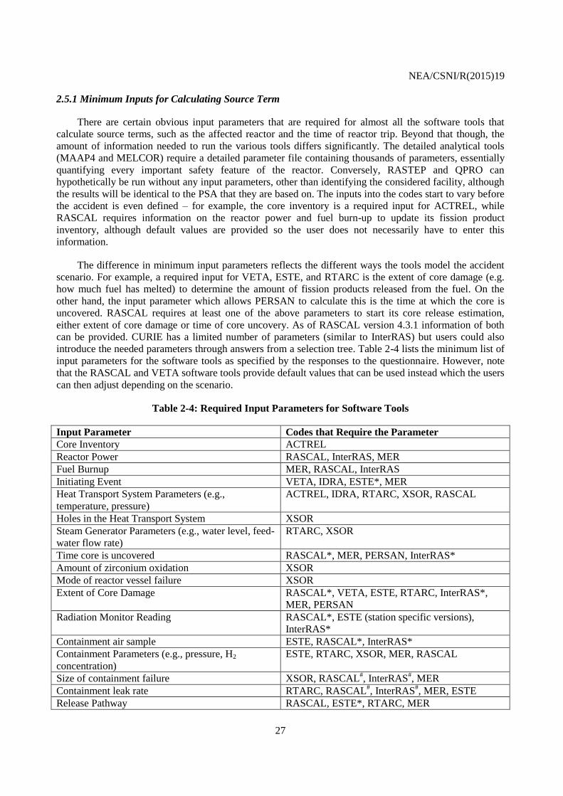
2.5.1 Minimum Inputs for Calculating Source Term
There are certain obvious input parameters that are required for almost all the software tools that
calculate source terms, such as the affected reactor and the time of reactor trip. Beyond that though, the
amount of information needed to run the various tools differs significantly. The detailed analytical tools
(MAAP4 and MELCOR) require a detailed parameter file containing thousands of parameters, essentially
quantifying every important safety feature of the reactor. Conversely, RASTEP and QPRO can
hypothetically be run without any input parameters, other than identifying the considered facility, although
the results will be identical to the PSA that they are based on. The inputs into the codes start to vary before
the accident is even defined – for example, the core inventory is a required input for ACTREL, while
RASCAL requires information on the reactor power and fuel burn-up to update its fission product
inventory, although default values are provided so the user does not necessarily have to enter this
information.
The difference in minimum input parameters reflects the different ways the tools model the accident
scenario. For example, a required input for VETA, ESTE, and RTARC is the extent of core damage (e.g.
how much fuel has melted) to determine the amount of fission products released from the fuel. On the
other hand, the input parameter which allows PERSAN to calculate this is the time at which the core is
uncovered. RASCAL requires at least one of the above parameters to start its core release estimation,
either extent of core damage or time of core uncovery. As of RASCAL version 4.3.1 information of both
can be provided. CURIE has a limited number of parameters (similar to InterRAS) but users could also
introduce the needed parameters through answers from a selection tree. Table 2-4 lists the minimum list of
input parameters for the software tools as specified by the responses to the questionnaire. However, note
that the RASCAL and VETA software tools provide default values that can be used instead which the users
can then adjust depending on the scenario.
Table 2-4: Required Input Parameters for Software Tools
Input Parameter Codes that Require the Parameter
Core Inventory ACTREL
Reactor Power RASCAL, InterRAS, MER
Fuel Burnup MER, RASCAL, InterRAS
Initiating Event VETA, IDRA, ESTE*, MER
Heat Transport System Parameters (e.g.,
temperature, pressure)
ACTREL, IDRA, RTARC, XSOR, RASCAL
Holes in the Heat Transport System XSOR
Steam Generator Parameters (e.g., water level, feed-
water flow rate)
RTARC, XSOR
Time core is uncovered RASCAL*, MER, PERSAN, InterRAS*
Amount of zirconium oxidation XSOR
Mode of reactor vessel failure XSOR
Extent of Core Damage RASCAL*, VETA, ESTE, RTARC, InterRAS*,
MER, PERSAN
Radiation Monitor Reading RASCAL*, ESTE (station specific versions),
InterRAS*
Containment air sample ESTE, RASCAL*, InterRAS*
Containment Parameters (e.g., pressure, H2
concentration)
ESTE, RTARC, XSOR, MER, RASCAL
Size of containment failure XSOR, RASCAL#, InterRAS
#, MER
Containment leak rate RTARC, RASCAL#, InterRAS
#, MER, ESTE
Release Pathway RASCAL, ESTE*, RTARC, MER

NEA/CSNI/R(2015)19
28
Input Parameter Codes that Require the Parameter
Release Height RASCAL, InterRAS, ESTE
Status of filters and sprays RASCAL, VETA, MER, PERSAN, XSOR,
InterRAS, ESTE
Status and amount of core that is involved in a high
pressure melt ejection
XSOR
Status of CCI XSOR
Amount of fuel that can participate in CCI XSOR
*,# - indicates that the software requires one of the input parameters listed, not all of them
2.5.2 Minimum Inputs for Calculating Doses
Compared to the tools that calculate source terms, the tools that estimate dispersion and doses have
much more in common with regards to what inputs they require. All require some form of meteorological
data and the location of the accident site, except for RASCAL which has generic, non-site specific
meteorological data available. Those tools that do not calculate source terms themselves (i.e., ARGOS,
MLDP, RODOS) need the source term as an input. Also, RASCAL provides user with an option to import
a source term calculated elsewhere and will calculate dispersion and doses.
For CURIE the distances for dispersion and dose calculations need to be specified, while RASCAL
and InterRAS provide doses at certain default distances which the user can then adjust. The dispersion and
dose results calculated by ESTE can also be updated based on readings from offsite radiation monitors.
2.5.3 Time Requirement
A critical parameter for these software tools is the time it takes them to run, as many would be used
by emergency response organisations where, in the event of an emergency, the assessment needs to be
carried out quickly. As a result, most of these software tools can be run in a matter of minutes or less.
CURIE, RASCAL, PERSAN, MER, QPRO, and InterRAS can all be run in under a minute. RTARC and
RASTEP can provide results almost instantaneously once all the input is provided. However, the time it
takes to run a software tool can depend on the amount of input that is provided as well as whether the basic
model or more in-depth module of the software tool is being run. For example, RASCAL can be run in
under a minute when analysing a release that is less than 24 hours in duration and using pre-defined, non-
site specific data is selected for the meteorological conditions. However, if the time frame for the analysis
is extended, say to 96 hours, and significant meteorological data is defined in RASCAL, the run time
increases but still remains affordable. On the other hand, MAAP4 was reported to be able to run in a few
minutes for simpler tasks. However, depending on the complexity of the input file and the nature of the
accident progression, a MAAP4 run can take several hours. Nevertheless, for running basic models with
minimum inputs, all the software tools have a run-time of fifteen minutes or less. It should be noted,
though, that no run-time was given for MELCOR in response to the questionnaire. Table 2-5 and Figure 2-
1 shows the minimum run-time of the software tools for which a run-time was specified. Note that for
Figure 2-1 a run-time of “a few minutes” was assumed to fall into the category of one to five minutes.
Table 2-5: Run-times for Software Tools
Code Minimum Run-Time
ABR Approximately 10 minutes for day of the accident duration
ACTREL 5 minutes
ARGOS (DEMA) At least 5 minutes
ARGOS (Health Canada) A few minutes
ASTRID 10 minutes for each day of accident progression

NEA/CSNI/R(2015)19
29
Code Minimum Run-Time
CURIE A few seconds
ESTE Source term – 1 minute
Dispersion and dose estimates – 5 minutes
IDRA 10 minutes
InterRAS Less than a minute
MAAP4 A few minutes
MC_Transport Seconds to minutes
MER A few seconds
MLDP 5 – 15 minutes (on a super-computer)
PERSAN Less than a minute
QPRO A few seconds
RASCAL Less than a minute
RASTEP Near Instantaneous
RODOS A few minutes (short-range calculations)
RTARC Near instantaneous
VETA 2 minutes
Figure 2-1: Minimum Run-Times for Software Tools
However, one should keep in mind that a fast run-time may be meaningless if it takes many hours to
set up all the input files for a run. The set up time can also vary significantly based how familiar the user is
with the software tool and the facility being modelled. However, several software tools can generally be set
up by a user of moderate familiarity with the software and be ready to run in less than ten minutes, such as
ESTE, VETA, RASTEP, RASCAL, PERSAN, and C3X. Others (RTARC and QPRO) can require up to 20
minutes to set up. Also, after an initial run, subsequent runs with many software tools, such as RASCAL
and QPRO are much quicker to set up.
0
1
2
3
4
5
6
7
8
1 min. or less 1 min. - 5 min. 5 min. - 10 min. 10 min. - 15 min.
# o
f C
od
es
Run-Times
Minimum Run-TIme of FASTRUN Codes

NEA/CSNI/R(2015)19
30
For ARGOS it is important to ensure that the source term data for input into the code should be in the
correct (XML) format. If it is in XML format and weather data is available on-line and can be downloaded
into ARGOS, then the tool can be run in a few minutes. If this information is provided in text format and
has to be entered into the code manually then the set up time can range from several minutes to an hour.
For RODOS, which uses also an XML source term input, an interface exists to QPRO. Using this interface
and online meteorological data, the input is done automatically. Similarly, if ASTRID has a direct link to
plant information, it can be ready to run within 5 minutes. However, manually entering data into ASTRID
extends the set up time to around 20 minutes. The longest set time is for MC_Transport. While the code
can run in only seconds to minutes, the minimum set up time is about an hour, but typically 4 – 8 hours are
needed to get intelligible results.
2.5.4 Software and Hardware Requirements
Most of the software tools require only to be installed on a Windows operating system to run;
however, the size of program size can vary significantly. VETA only takes 1 MB of storage space,
RASCAL requires 75 MB, and RTARC requires a minimum of 2 GB of RAM and a 500 GB hard disk
drive. An ESTE server requires 8 to 12 GB of RAM and a hard disk drive of 40 to 80 GB. The most
demanding software tool is MLDP which requires a supercomputer to run.
2.5.5 User Training
The amount of training need to run the various software tools varies significantly. CURIE, QPRO,
and RASTEP are designed to be easy to use so only a short, basic training session is needed, and users of
MC_Transport receive only on the job training. Conversely, ARGOS requires extensive training to use and
IDRA is meant to only be used by the nuclear power plant experts. Table 2-6 shows the training
requirements different organisations have for using their software tools. Note that the tools identified in the
table are only the ones for which training requirements were specified in the response to the questionnaire.

NEA/CSNI/R(2015)19
31
Table 2-6: User Training Associated with Software Tools
Organisation Software Tools User Training Required
ABmerit ESTE 2 day training course and continuous practice or (yearly)
repeated training
Areva MC_Transport On the job training
Bel V CURIE Short training course and on the job training
DEMA ARGOS 3 – 4 day training course
GRS QPRO Minimal training
Health Canada ARGOS and MLDP Extensive training
IAEA InterRAS Minimal training
IRSN MER and PERSAN Short training course for both tools, each with
description of models
KIT RODOS 2 days training course, remote training of basic modules
possible
NPCIL ACTREL One day hands on training (however, full familiarity to
come after 2 to 3 months experience)
SSM RASTEP Basic training
USNRC RASCAL 1.5 days training
2.6 Software Output
2.6.1 Source Term Output
The source terms calculated by the software tools vary significantly in terms of what materials are
considered in the source term. Indeed, some software tools provide a source term broken down by
radionuclide (RASCAL, VETA, ACTREL, ESTE, RTARC, RASTEP, InterRAS, MER), others provide a
source term broken down by chemical element groups (MER, PERSAN, XSOR, MELCOR, MAAP4), and
some tools provide a radionuclide breakdown for some elements but not all (CURIE, PERSAN). Also,
when the release is broken by element groups, some tools express the release in units of activity (CURIE,
PERSAN), other express it in units of mass (MELCOR, MAAP4, IDRA, MER). Some software tools only
calculate releases for four radionuclides/elements (CURIE), while others report releases for up to 70
radionuclides (RASCAL, InterRAS). In fact, RASCAL and MER can consider up to 150 radionuclides in
the source term and dose calculations and have over 800 in its database. However, there are three element
groups that all the software tools report in their source terms: noble gases, iodine, and caesium. For
software tools that provide an isotopic breakdown of their source terms, they all include the following
radionuclides: Xe-133, I-131, and Cs-137. Another element that is included in the source terms of all but
two of the software tools is tellurium, with Te-132 present in all codes where the radionuclides are
specified. Table 2-7 shows all the elements that are considered in at least two software tools, which tools
include them in their source terms, and which radionuclides of the elements are considered.

NEA/CSNI/R(2015)19
32
Table 2-7: The Elements and Radionuclides Considered in the Source Terms Calculated by Fast
Running Software Tools
Element Radionuclides
Considered
Codes
Caesium Cs-134 RASCAL, VETA, ESTE, PERSAN, MER
Cs-136 RASCAL, VETA, ESTE, PERSAN, MER
Cs-137* RASCAL, VETA, ESTE, CURIE, RASTEP, PERSAN,
MER
Cs-138 RASCAL, ESTE, PERSAN, MER
General Cs release MER, PERSAN, XSOR, MELCOR, RASCAL
Iodine I-131 RASCAL, VETA, ESTE, CURIE, RASTEP, PERSAN,
MER
I-132 RASCAL, VETA, ESTE, PERSAN, MER
I-133 RASCAL, VETA, ESTE, CURIE, PERSAN, MER
I-134 RASCAL, VETA, ESTE, PERSAN, MER
I-135 RASCAL, VETA, ESTE, PERSAN, MER
General I release MER, PERSAN, XSOR, MELCOR, RASCAL
Xenon Xe-131m RASCAL, VETA, PERSAN, MER
Xe-133 RASCAL, VETA, ESTE, PERSAN, RASTEP, MER
Xe-133m RASCAL, VETA, ESTE, PERSAN, MER
Xe-135 RASCAL, VETA, ESTE, PERSAN, MER
Xe-135m RASCAL, ESTE, PERSAN, MER
Xe-138 RASCAL, VETA, ESTE, PERSAN, MER
General Xe release CURIE, PERSAN, XSOR, MELCOR, PERSAN, MER
Tellurium Te-127 RASCAL, ESTE, PERSAN, MER
Te-127m RASCAL, PERSAN, MER
Te-129 RASCAL, ESTE, PERSAN, MER
Te-129m RASCAL, VETA, ESTE, PERSAN, MER
Te-131 RASCAL, PERSAN, MER
Te-131m RASCAL, VETA, ESTE, PERSAN, MER
Te-132 RASCAL, VETA, ESTE, PERSAN, RASTEP, MER
General Te release PERSAN, XSOR, MELCOR, MER
Krypton Kr-83m RASCAL, PERSAN, MER
Kr-85 RASCAL, VETA, ESTE, PERSAN, MER
Kr-85m RASCAL, VETA, ESTE, PERSAN, MER
Kr-87 RASCAL, VETA, ESTE, PERSAN, MER
Kr-88 RASCAL, VETA, ESTE, PERSAN, MER
General Kr release CURIE, PERSAN, MER, MELCOR
Ruthenium Ru-103 RASCAL, VETA, ESTE, MER
Ru-105 RASCAL, VETA, ESTE, MER
Ru-106* RASCAL, VETA, ESTE, MER
General Ru release MER, XSOR, MELCOR
Barium Ba-139 RASCAL, MER
Ba-140 RASCAL, VETA, ESTE, MER
General Ba release XSOR, MELCOR, MER
Cerium Ce-141 RASCAL, ESTE, MER
Ce-143 RASCAL, ESTE, MER
Ce-144* RASCAL, VETA, ESTE, MER

NEA/CSNI/R(2015)19
33
Element Radionuclides
Considered
Codes
General Ce release XSOR, MELCOR, MER
Lanthanum La-140 RASCAL, VETA, ESTE, MER
La-141 RASCAL, MER
La-142 RASCAL, MER
General La release XSOR, MELCOR, MER
Molybdenum Mo-99 RASCAL, VETA, RASTEP, ESTE, MER
General Mo release MELCOR, MER
Strontium Sr-89 RASCAL, VETA, ESTE, MER
Sr-90 RASCAL, VETA, ESTE, MER
Sr-91 RASCAL, VETA, ESTE, MER
Sr-92 RASCAL, MER
General Sr release XSOR, MER, MELCOR
Antimony Sb-127 RASCAL, VETA, ESTE, MER
Sb-129 RASCAL, VETA, ESTE, MER
Rubidium Rb-86 RASCAL, ESTE, MER
Rb-88 RASCAL, RASTEP, ESTE, MER, MELCOR
Yttrium Y-90 RASCAL, ESTE, MER
Y-91 RASCAL, VETA, ESTE, MER
Y-91m RASCAL, ESTE, MER
Y-92 RASCAL, MER
Y-93 RASCAL, MER, MELCOR
* indicates that the radionuclide has a short-lived daughter whose activity is included in the parent
radionuclide
Some notes on Table 2-7: both RTARC and ACTREL indicated in the response to the questionnaire
that they provide a source term broken down by radionuclide. However, the radionuclides that they
consider are not specified. It is indicated though that RTARC considers 56 specific radionuclides and the
source term it produces is based on MELCOR results. As for ACTREL it includes radionuclides of Cs, I,
Xe, Kr, Te and Sr in its source term. MER can evaluate all released radionuclides if these radionuclides are
present in the core inventory. An advanced user can select the radionuclides (s)he is interested in. Finally,
MC_Transport, ASTRID, QPRO, and IDRA do not indicate which radionuclides/elements they include in
their source term.
In addition to having a variety of radionuclides and elements considered in the source terms, the
output format of the different software tools varies as well. Many codes display the source term in tables
with most of those also displaying graphs. The output from other software tools is in the form of text files.
RASTEP is unique in that it shows the probability of several source terms as an output. See Table 2-8 for
the source term output format of the software tools.
Table 2-8: Output Formats of the Software Tools that Calculate Source Terms
Code Source Term Reporting Format
ACTREL Tables, Graphs
ASTRID Tables
CURIE Tables
ESTE Tables, Graphs, XML files, text files
IDRA Tables, Graphs

NEA/CSNI/R(2015)19
34
InterRAS Tables, Graphs
MAAP4 Tables, Text files
MC_Transport Text files
MELCOR Tables, Graphs
MER Text files exportable to Excel
PERSAN Tables, Graphs, Test files, HDF5 files
QPRO Graphs
RASCAL Tables, Graphs, Summary reports, text files in XML or CSV
formats
RASTEP Graphs
RTARC Tables, Graphs, Summary report
VETA Text files
XSOR Text files
There is one commonality amongst the source terms most tools estimate: the source term is time
dependent. One software tool reported (CURIE) that they only calculate the total radionuclide release over
the entire accident duration. However, another two software tools (VETA and XSOR) provide a source
term at certain stages of the accident progression, rather than as a direct function of time.
The time duration of a release that can be calculated varies significantly between the software tools
but all of the tools can calculate and track a release for at least 48 hours. Four software tools:
MC_Transport, IDRA, ESTE, and MAAP4 can hypothetically calculate a release of infinite duration.
Some software tools that do not estimate doses also format their output so that it can be easily used by
dispersion tools. The output of MC_Transport can be imported into MACCS, ASTRID and QPRO’s
outputs can be used as inputs to RODOS, RASTEP is being developed so that it can input into ARGOS,
PERSAN outputs can be used as inputs to C3X, and there are ancillary routines to VETA allowing its
source term to be inputted into RASCAL.
2.6.2 Dose Prediction
Similar to the time duration over which releases can be calculated, there is significant variation in the
distance over which the dispersion and dose software tools can track the plume. The distance over which
every software tool can calculate dispersion and dose is up to 15 km. However, all but one of these
software tools can estimate doses out to at least 80 km (50 miles), and the one tool with the 15 km
calculation limit can extrapolate beyond 15 km. Four software tools; ARGOS, MLDP, ESTE, and C3X,
reported on the questionnaire that they can track releases worldwide. Also, it was stated that ESTE and
C3X did successfully track releases from Fukushima to the central Europe. RODOS also has a world wide
data base and can be used everywhere.
When predicting doses, almost all of the software tools are able to superimpose the resulting doses
from the plume over a map of the affected region. Furthermore, several software tools have information on
the local demographics (population near the reactors): ARGOS (for Denmark), RODOS, ESTE, and
RASCAL. ESTE even has an age breakdown for the nearby villages; calculating doses for those 0-1, 1-10,
10-18, 18-60, and greater than 60-years old. While RTARC does not have demographics built in, it does
consider doses for six different age groups: infants (0-1 years old), children 1-2 years old, 2-7 years old, 7-
12 years old, 12-17 years old, and adults. ABR also assesses doses for six different age groups as required
by German law.

NEA/CSNI/R(2015)19
35
The exposure pathways used to calculate doses are similar for all the tools, as each one looks at doses
due to cloudshine, groundshine and inhalation. Six software tools also assess doses via ingestion: ARGOS,
MLDP, C3X, RODOS, ACTREL, and InterRAS. ACTREL specifies that the ingestion dose pathway it
considers is milk from cows eating contaminated grass, while RASCAL’s Field Measurement to Dose
module can be compared to Derived Intervention Levels for food and other products. Some information
was provided as to which organs doses the software tools could calculate. ARGOS, CURIE, C3X,
RASCAL and RODOS identified organ doses: all can calculate thyroid dose, RASCAL and C3X can
calculate doses to the lungs, colon, and bone, while RODOS calculates doses for 11 different organs.
Several software tools provide recommendations for protective actions based on the dose results.
CURIE, RODOS, ESTE, C3X, and RTARC all provide recommendations as to when to shelter, when to
evacuate, and when to distribute stable iodine pills based on the calculated doses. CURIE also provide a
recommendation regarding food bans in connection with a derived reference I-131 or Cs-137 ground
deposition (in Bq/m²). RODOS recommends whether food restrictions need to be enacted. Finally, while
not recommending protective actions, RASCAL and InterRAS do indicate when calculated doses exceed
Protective Action Guidelines of the U.S EPA (RASCAL) or the IAEA (InterRAS). The reference dose
levels in CURIE are based on the Belgian Emergency Plan, while those in RTARC come from Slovakian
law. However, both RODOS and ESTE are used in multiple countries. RODOS has country specific action
levels programmed in. With ESTE, as well as with C3X, users enter the dose threshold for sheltering,
evacuation, and KI distribution according to the legislation in the user’s country.
2.7 Validation
For calculating source terms, the majority of the fast running software tools were validated based on
comparing results with more detailed, analytical software tools: mainly ASTEC, MAAP4, and MELCOR.
As a result, the source terms that the fast running codes predict are expected to be within the same order of
magnitude as those calculated by the detailed codes; for example, VETA’s results were within 8% of the
MAAP4 results it was being validated against. Certain fast-running software tools were also validated
against other fast-running software tools. The IRSN validated their two fast running tools MER and
PERSAN against each other, as well as validating both against ASTEC. The RASCAL algorithms have
also been validated through inter-model comparisons. See NUREG-1940 and NUREG/CR-6853. ABmerit
compared ESTE against ASTEC, MELCOR, PC Cosyma, TAMOS (ZAMG - Zentralanstalt für
Meteorologie und Geodynamik, Vienna, Austria) and another Slovak code: RTARC. Table 2-9 shows the
detailed analytical tools that fast running software tools were validated against.

NEA/CSNI/R(2015)19
36
Table 2-9: Codes used to Validate Fast Running Software Tools
Software Tool Analytical Tool Used for Validation
ACTREL MELCOR
ASTRID ASTEC
ESTE ASTEC, MELCOR, RTARC, TAMOS, PC
COSYMA
IDRA ASTEC, MELCOR
MER ASTEC, PERSAN
PERSAN ASTEC, MER
RASCAL MAAP5, MELCOR, RATCHET, ADAPT/LODI,
TurboFRMAC-2011
RASTEP MAAP4, MELCOR
RTARC ASTEC, MELCOR
VETA MAAP4 (specifically MAAP4-CANDU)
XSOR MAAP4, MELCOR
The integral codes themselves (MAAP4 and MELCOR) were validated against experimental results
as well as previous accidents such as Three Mile Island. A couple of the faster running software tools were
validated against experimental results as well. ACTREL’s thermal hydraulics models were validated
against experimental results available to NPCIL.
Of course, some organisations also used their software tools to calculate the releases from Fukushima
during and immediately after the accident, before more detailed models could be established. RASCAL is
being benchmarked in a comprehensive US study of several emergency response codes using actual
Fukushima field data and comparative analyses.
It must be stressed that discrepancies, sometimes significant, will always be present when trying to
use software tools to predict complex phenomena. This is especially true when trying to estimate
something as inherently complex as a severe accident at a nuclear facility, where a single operator action or
system functioning can completely change the nature of the event. For example, when ASTRID was
validated against the experimental results, in some cases its calculations were found to be off by as much
as a factor of 20. Therefore, its uncertainty is quoted at two orders of magnitude. Uncertainty of other code
predictions for the atmospheric dispersion can also be significant, especially for complex atmospheric
phenomena.
The software tools used to model dispersion tend to be validated against experimental results as well
as actual events. Sometimes these experiments and events do involve the release of nuclear material. The
dispersion models in ESTE were validated by a Czech experiment that released Tc-99m into the
atmosphere and part of RTARC dispersion validation was based on multi-tracer atmospheric tests
performed by Idaho National Engineering Laboratories. RASCAL’s atmospheric dispersion and deposition
algorithms were adapted from the RATCHET model and have undergone extensive peer review validation
against field measurements as part of the Hanford Environmental Dose Reconstruction (HEDR) project.
Almost all dispersion tools were used to model the plumes from Fukushima. Other organisations have used
non-nuclear releases as part of their validation, as a particulate releases will be affected by dispersion the
same way whether it is radioactive or not. Environment Canada used forest fires and volcanic eruptions as
part of the validation process for MLDP.

NEA/CSNI/R(2015)19
37
In over 50% of the validation experiments VUJE carried on RTARC dispersion models, the results
were within a factor of 2. The dose rate estimations done for Fukushima by C3X were found to be within a
factor of 5 of those measured over Japan using source terms from PERSAN or MER made during the
response.
2.8 Summary
Table 2-10 provides a high level overview of the capabilities of the software tools presented in this
benchmarking used to calculate source terms. Only information which relates to the code’s ability to
estimate the source term is presented in Table 2-10. A similar overview for the codes used to calculate
dispersion and doses is presented in Table 2-11. In Table 2-11 software tools that do not list the source
term in the minimum input are capable of calculating source terms themselves.
Note that the information is based on the responses to the questionnaire. The blank spaces indicate
that the information was not provided in the questionnaire.

NEA/CSNI/R(2015)19
38
Table 2-10: High level overview of fast-running software tools used to calculate source terms
Software Main
Algorithm
Reactors Types
Modelled
Specific Reactors Modelled
Hydrogen Combustion Modelling
Multi-unit
Modelling
Reduction Mechanisms
Modelled Minimum Information
Needed to Run Set-up Time Run Time
ACTREL PHWR N/A No Yes
Filters, Sprays, Natural deposition
Thermal-hydraulic data, Core inventory
5 minutes
ASTRID
Uses a simplified model based on a deterministic safety analysis
BWR, PWR
N/A Yes No
Retention in RCS, Filters, Sprays, Pool scrubbing, Iodine chemistry
Requires significant input including: Plant geometry, Status of safety systems, Temperature in containment, Pressure in containment, Water level in containment
5 min. with link to NPP, 20 min. typing
10 min. for each day being modelled
CURIE V5 Arithmetic Expression
PWR All Belgian reactors
No Yes
Filters, Sprays, Partition factor (SGTR), Natural deposition
Time of reactor trip, Noble gas, I, and Cs releases: can be based on event tree selections
A few seconds

NEA/CSNI/R(2015)19
39
Software Main
Algorithm
Reactors Types
Modelled
Specific Reactors Modelled
Hydrogen Combustion Modelling
Multi-unit
Modelling
Reduction Mechanisms
Modelled Minimum Information
Needed to Run Set-up Time Run Time
ESTE Based on previous analysis
BWR, PWR, PHWR, Gas reactors, Research reactors, Spent fuel pools
All Slovakian, Czech, and Bulgarian reactors
No Yes
Sprays, Filters, Natural deposition, Pool scrubbing, Leakage
Assuming there's no link to the reactor the following information is needed: Location, Release pathway, State of the reactor core, State of containment
5 minutes at most
60 sec. for basic source term, 10-15 min. for more detail
IDRA Method of moments
BWR, PWR, Sodium reactors, Research Reactors
N/A Yes No Filters, Sprays
Type of accident, Plant configuration
Less than 10 minutes
InterRAS Arithmetic Expression
BWR, PWR, Spent fuel pools
N/A No No
Sprays, Filters, pool scrubbing, Natural deposition, partition factor (SGTR)
Time of shut down, Time and duration of core uncovery, Containment hold-up time, Reduction parameters Release pathway, Use of filters
Less than 30 seconds

NEA/CSNI/R(2015)19
40
Software Main
Algorithm
Reactors Types
Modelled
Specific Reactors Modelled
Hydrogen Combustion Modelling
Multi-unit
Modelling
Reduction Mechanisms
Modelled Minimum Information
Needed to Run Set-up Time Run Time
MAAP 4.0.8 Requires parametric plant model
BWR, PWR
N/A Yes No
Sprays, Filters, Pool scrubbing, Natural deposition, Partition factor (SGTR)
Parametric plant model A few minutes
MC_Transport
Uses a simplified model based on a deterministic safety analysis
Any N/A No Yes
Filters, Natural deposition, Flow rates
Deterministic calculation of a similar accident scenario
4 - 8 hours
Seconds to minutes
MELCOR 1.8.4 Requires parametric plant model
BWR, PWR
N/A Yes No Filters, Sprays
Parametric plant model
MER Mass balance equations
PWR All French Reactors
No No
Sprays, Filtered venting, Leakage, Natural deposition, Iodine trapped by silver in the sump
Reactor type, Fuel characteristics, Basemat composition, Time of trip, Time RCS break occurred, Time core is uncovered, Status of safety systems,
5 minutes (more time in expert mode)
A few seconds

NEA/CSNI/R(2015)19
41
Software Main
Algorithm
Reactors Types
Modelled
Specific Reactors Modelled
Hydrogen Combustion Modelling
Multi-unit
Modelling
Reduction Mechanisms
Modelled Minimum Information
Needed to Run Set-up Time Run Time
Best estimate or Monte-Carlo
PERSAN Arithmetic Expression
PWR All French Reactors
No, but interacts with a code that can
No
Sprays, Filtered venting, Leakage, Natural deposition
Reactor type, Time of trip, Time RCS break occurred, Time core is uncovered, Status of safety systems
About 5 minutes
Less than a minute
QPRO Based on Level 2 PSA
Any N/A
Yes, if PSA contain hydrogen analysis
If a multi-unit PSA exists, then yes
All mechanisms considered in the PSA
Only the PSA is needed to run but the output would then be the same as the PSA. Other data adjusts the scenario.
20 min. for the 1st run
A few seconds
RASCAL 4.3.1
Arithmetic expression plus based on some previously analyzed events
BWR, PWR, Spent fuel pools
All American reactors, Laguna Verde
No Yes
Sprays, Filters, Pool scrubbing, Natural deposition, Partition
Time of shut down, Time and duration of core uncovery, Containment hold-up time, Reduction parameters Release pathway,
Less than 15 min. for 1st run
Typically less than a minute

NEA/CSNI/R(2015)19
42
Software Main
Algorithm
Reactors Types
Modelled
Specific Reactors Modelled
Hydrogen Combustion Modelling
Multi-unit
Modelling
Reduction Mechanisms
Modelled Minimum Information
Needed to Run Set-up Time Run Time
factor (SGTR)
Use of filters
RASTEP
Bayesian belief network (BBN) based on Level 2 PSA
BWR, soon PWR
Oskarshamn, soon Ringhals
No No
Mechanisms considered in the PSA are modelled as BBN nodes
Only the PSA is needed to run but the output would then be the same as the PSA. Other data adjusts the scenario.
5 - 10 minutes
Near instantaneous
RTARC Based on previous analysis
PWR N/A No No
Mechanisms considered in previous scenarios
See the list following this table
10 - 20 minutes
A few seconds
VETA Arithmetic Expression
PHWR All Canadian reactors
No Yes
Sprays, Filters, Natural deposition
Event location, Time of shutdown, Is the accident a LOCA (Y/N), How much of the core is damaged and when, When did the first release occur and was it filtered
2 minutes
Less than 2 minutes

NEA/CSNI/R(2015)19
43
Software Main
Algorithm
Reactors Types
Modelled
Specific Reactors Modelled
Hydrogen Combustion Modelling
Multi-unit
Modelling
Reduction Mechanisms
Modelled Minimum Information
Needed to Run Set-up Time Run Time
XSOR Arithmetic Expression
PWR All Korean PWRs, Surry
No No
Sprays, Pool scrubbing, Natural deposition, Partition factor (SGTR)
See the list following this table
A very short time
When running XSOR, the following parameters need to be defined:
Fraction of radionuclide i released into the reactor vessel, prior to vessel breach
Fraction of radionuclide i entering the steam generator
Fraction of radionuclide i released from the steam generator to the environment
Fraction of radionuclide i released from the cooling system into the vessel
Fraction of material that escapes containment at or prior to vessel breach, before consideration of decontamination mechanisms
Decontamination factor for coolant system release prior to or at vessel breach
Fraction of the core material involved in a pressurised melt ejection
Fraction of radionuclide i released to containment following a pressurised melt ejection, due to direct heating
Fraction of the material participating in MCCI
Fraction of material remaining in the reactor vessel after a breach that can be revolatilised later
Fraction of radionuclide i participating in core – concrete interaction (CCI) that remains in the debris
Fraction of radionuclide i released during CCI that escapes containment
Decontamination factor applicable to CCI release
Fraction of radionuclide i that remains in the cooling system after the vessel breach, but will be revolatilised later
Fraction of the revolatilised radionuclide i the is released from containment before consideration for decontamination mechanisms
When running RTARC, typically 5 to 10 of the following parameters need to be defined:
Parameters of primary circuit such as:
o core outlet temperature
o pressure in the primary circuit

NEA/CSNI/R(2015)19
44
o emergency core cooling system flow rates
o volume activity in primary circuit
o neutron flux
Parameters of secondary circuit such as
o steam pressure in secondary circuit
o water level in the steam generators
o normal and emergency feed water flow rate
o volume activity in secondary circuit
Parameters of hermetic spaces (containment) such as
o total pressure
o temperature
o hydrogen concentration
o dose rate
o noble gases volume activity
o spray system flow rate etc.
Parameters beyond containment boundary (needed for identification of containment “by-pass” scenarios) such as
o activity in reactor hall
o coolant activity in embedded cooling system of the MCPs and in Reactor Protection and Regulation system

NEA/CSNI/R(2015)19
45
Table 2-11: High level overview of fast-running software tools used to calculate doses
Software Dispersion
Model Range Local
Demographics Exposure Pathways
Organ Doses
Recommended Protective
Actions
Minimum Information
Needed to Run Set-up Time Run Time
ABR Lagrangian 500 km No Inhalation, Cloudshine, Groundshine
TEDE, Thyroid
Release location, Source term, Meteorological data, Topography, Area of interest, Time step size
Less than a minute for basic calculations with automatic data More complex runs and manual input take longer
1 minute for each time step (typically set at 1 hour)
ACTREL Gaussian plume
100 km No
Inhalation, Cloudshine, Groundshine, Ingestion
TEDE, Thyroid
None
Meteorological data, Dose conversion factors
5 minutes
ARGOS Gaussian puff (RIMPUFF), Lagrangian
100 km for RIMPUFF, Lagrangian model is unlimited
Yes (as used by DEMA)
Inhalation, Cloudshine, Groundshine, Ingestion
TEDE, Thyroid
None built in but can be defined by user
Radionuclides released, Release height, Release location, Duration of release, Meteorological data
5 minutes (with source term and met data load directly into code) to 60 minutes (all manual input)
5 - 15 minutes
C3X 4D Gaussian puff 4D Eulerian
Unlimited No
Inhalation, Cloudshine, Groundshine, Ingestion
TEDE, Thyroid, Bone, Colon,
Evacuation, Sheltering, KI distribution, Food
Source term (from PERSAN) Meteorological data
5 minutes
Depending on the area to be covered &

NEA/CSNI/R(2015)19
46
Software Dispersion
Model Range Local
Demographics Exposure Pathways
Organ Doses
Recommended Protective
Actions
Minimum Information
Needed to Run Set-up Time Run Time
Lungs inspection
the duration
of the
release,
few
minutes
for typical
small-
scale
dispersion
and doses
CURIE V5 Gaussian
15 km (but can be extrapolated further)
No Inhalation, Cloudshine, Groundshine
TEDE, Thyroid
Evacuation, Sheltering, KI distribution, Food inspection
Wind speed class, Release height, Release location
A few seconds
ESTE Gaussian puff, Lagrangian
Usually 200-300 km, but can be extended globally
Yes Inhalation, Cloudshine, Groundshine
TEDE, Thyroid
Evacuation, Sheltering, KI distribution
Meteorological data
1 - 5 minutes 5 minutes
InterRAS Gaussian plume, Gaussian puff
80 km Yes
Inhalation, Cloudshine, Groundshine, Ingestion
TEDE, Thyroid, Bone, Colon, Lungs
None, but does indicate when doses exceed Preventative Action Guidelines
Release height, Duration of release, Meteorological data
15 minutes Typically less than a minute

NEA/CSNI/R(2015)19
47
Software Dispersion
Model Range Local
Demographics Exposure Pathways
Organ Doses
Recommended Protective
Actions
Minimum Information
Needed to Run Set-up Time Run Time
MLDP
Lagrangian (Canadian Meteorological Centre (CMC) model)
Unlimited No
Inhalation, Cloudshine, Groundshine, Ingestion
TEDE, Thyroid
None
Radionuclides released, Release height, Release location, Duration of release, Meteorological data
10 minutes (with source term and met. data load directly into code) to 60 minutes (all manual input)
5 - 15 minutes
RASCAL 4.3.1
Gaussian plume, Lagrangian-Gaussian puff
160 km Yes Inhalation, Cloudshine, Groundshine
TEDE, Thyroid, Bone, Colon, Lungs
None, but does indicate when doses exceed Protective Action Guidelines
Duration of release 15 minutes Typically less than a minute
RODOS
Gaussian puff (ATSTEP, RIMPUFF), Lagrangian (DIPCOT), Eulerian (MATCH)
100 km to unlimited
Yes, global population with 10 km resolution
Inhalation, Cloudshine, Groundshine, Ingestion, Skin exposure
TEDE, Thyroid, Skin, and 8 others
Evacuation, Sheltering, KI distribution, Food inspection
Source term, Meteorological data, Release location, Area of interest
Less than 10 minutes with data automatically loaded into the code, 40 minutes for manual input
15 minutes
RTARC Gaussian plume, Gaussian puff
40 km for Gaussian plume, Gaussian puff can model Europe
Can be added Inhalation, Cloudshine, Groundshine
TEDE, Thyroid
Evacuation, Sheltering, KI distribution
Release height, Duration of release, Meteorological data
10 -20 minutes
A few minutes

NEA/CSNI/R(2015)19
48

NEA/CSNI/R(2015)19
49
3 DESCRIPTION OF MODELLED SCENARIOS
Five different hypothetical accident scenarios were used in the benchmarking modelling. They were
selected to allow sufficient representation of various reactor technologies, including the most widespread
types of reactors, as well as diverse severe accident progressions s that involved significant core
degradation:
An unmitigated, long-term station blackout at Peach Bottom Unit 3, an American BWR
An unmitigated, long-term station blackout at Surry Unit 1, an American PWR
A transient resulting in a loss of residual heat removal at Oskarshamn Unit 3, a Swedish BWR
A large break LOCA with failure of safety functions at Golfech Unit 1, a French PWR
A station blackout with emergency power generators at Point Lepreau, a Canadian PHWR
This section presents the accident scenarios used in this benchmarking exercise. The scenarios were
at some point modelled using detailed, analytical software tools. The Peach Bottom and Surry accident
scenarios were modelled with MELCOR, the Golfech scenario was modelled with ASTEC, and the Point
Lepreau scenario was modelled with MAAP4-CANDU. Note that while MAAP4 was used to analyse the
Point Lepreau scenario, it was also used as one of the tools to simulate the Peach Bottom and Surry
scenarios. The progression of the hypothetical severe accidents as determined by the detailed, analytical
software tools will be discussed as well as the calculated releases. The radionuclide releases to the
atmosphere that are estimated by these analytical tools serve baselines for comparing source terms
estimated by the fast-running software tools.
A detailed, documented description of the Oskarshamn scenario was not available, so the details of
the accident progression were obtained through correspondence with members of the SSM. The RASTEP
software was designed specifically for Oskarshamn, based on the reactor’s PSA. Therefore, source terms
calculated for the Oskarshamn scenario by other participants were compared to source terms predicted by
RASTEP.
For each scenario three different datasets were presented. These datasets are meant to represent the
different amount of information that would be available to emergency response organisations at different
times during accident progression. The three datasets are as follows:
1 hour into the accident scenario, when only the reactor location and initiating event are known;
6 hours into the accident scenario, when data on core cooling is available along with additional
information on the accident scenario;
It is important to remember that the accident scenarios used in this benchmarking exercise are
simplified and hypothetical. For the purposes of this project, the considered accident scenarios were
deliberately designed to involve significant core degradation. The likelihood of such events was not
considered; in fact, due to the design modifications undertaken in response to the Fukushima
experience, such accidents may be so unlikely to be considered out of the realm of possibility. They
should in no way be considered as events that will happen during the operating life of the reactors.

NEA/CSNI/R(2015)19
50
24 hours into the accident scenario, when the status of containment and other key information is
known.
The purpose of having three different datasets each with varying amounts of information available is
to examine how well different software tools cope with a limited amount of information.
In addition to the limited information on accident progression, all participants were provided with
meteorological data for each accident scenario so that plume dispersion could be modelled. The
meteorological data is representative of real weather conditions at and nearby the reactor sites on certain
dates. The weather data for all the LWR scenarios were provided by ABmerit, who retrieved the data
from the National Oceanic and Atmospheric Administration’s (NOAA) weather server. The
meteorological data for the Point Lepreau scenario was taken from the Weather Network and was
provided to the participants by the CNSC. The meteorological data used for the accident scenarios is
presented in Appendix B.
3.1 Peach Bottom
3.1.1 Accident Progression
The American BWR scenario was taken from the USNRC's State of the Art Reactor Consequence
Analyses report. The selected scenario from the report was the long-term, unmitigated station blackout at
Peach Bottom caused by an earthquake. “Long-term” does not indicate the duration of the blackout, rather
it refers to the fact that significant core damage occurs in the long-term [11-2].
The scenario is not a complete station blackout, at least not immediately. DC power is available from
the batteries for the first four (4) hours of the accident (after operators shed non-essential loads); however,
no AC power is available as the diesel generators do not start. With DC power available, the reactor core
isolation cooling (RCIC) system starts automatically to make up lost coolant inventory and maintain the
water level in the reactor pressure vessel (RPV). One hour into the accident, operators manually open a
safety relief valve (SRV) to start a controlled depressurisation of the RPV, and an hour later the operators
take over remote manual control of the RCIC system. Once the batteries are drained, the open SRV closes
and water in the RPV increases. The RCIC does not stop until 5.2 hours into the accident, at which point
the rising water level floods the steam line to the RCIC turbine. An hour after RCIC stops, the coolant
reaches saturation temperature, increasing pressure in the RPV. At 6.4 hours, the rising pressure forces
the SRV back open. The SRV then cycles open and closed, discharging coolant, until at 8.2 hours it sticks
open, increasing the rate of coolant discharge and bringing the RPV pressure into equilibrium with
containment after 2 hours. With an open release path, the RPV water level decreases quickly. At about 8.5
hours, , the water level has fallen below the top of the active fuel and about one hour later, the water level
is below the bottom of the lower core plate [11-2].
As the core becomes exposed, it heats up and starts to melt. At 10.5 hours into the accident, the
lower core plate fails and the fuel debris relocates into the lower head of the RPV. The fuel debris is
temporarily cooled by the water remaining in the lower head, but after the remaining water is boiled off at
13.3 hours, the debris heats up again. As the core was being uncovered, the steam and heat in the core
caused oxidation of the Zircaloy fuel cladding. This oxidation produced significant quantities of hydrogen
gas (900 kg between 9 – 19 hours), with most of the hydrogen being generated before the lower head
dried out. This hydrogen leaked through the open SRV into the primary containment (dry well) and
subsequently into the reactor building via the dry well flange.

NEA/CSNI/R(2015)19
51
At 20 hours into the accident scenario the hydrogen in the reactor building ignites. The resulting
pressure blows out panels in the wall of the refuelling bay, opening the reactor building to the
environment. Additional hydrogen burns occur, blowing open several access doors, including a large
railroad access door. At about 20 hours after the accident started, the final barriers to prevent large scale
fission product release have failed [11-2].
Table 3-1 shows a summary of the Peach Bottom accident scenario that was provided to the
participants for them to use to model the accident scenario with their software tool(s). Note that three
different datasets are represented by the table, depending on when information is first available.
Table 3-1: Summary of the Peach Bottom Accident Scenario
Parameter Time
Information is Available
Parameter Value
Reactor name 1 hour after accident
Peach Bottom
Reactor design 1 hour after accident
General Electric BWR with Mark I containment
Thermal power 1 hour after accident
3514 MWth
Brief description of the accident
1 hour after accident
Unmitigated long-term station blackout caused by 0.3-0.5 g peak ground acceleration earthquake; resulting in the loss of all AC power One safety relief is opened to reduce pressure at 1 hour Operators take manual control of RCIC (Reactor Core Isolation Cooling) after 2 hours
Reactor shutdown (Yes/No)
1 hour after accident
Yes
If yes, time of reactor shut down
1 hour after accident
< 15 minutes
Power Available (Yes/No)
6 hours after accident
No AC or DC power available at 6 hrs (AC power lost at 0:00 and batteries depleted at 4:00)
Core uncovered/Loss of heat sinks (Yes/No)
6 hours after accident
No. Core still covered at 6 hrs

NEA/CSNI/R(2015)19
52
3.1.2 Radionuclide Release
In this scenario, the release of fission products from the core starts at about 9.1 hours, when the top
third of the core has been uncovered. However, no significant release to the environment occurs until 20
hours. Release of radionuclides to the atmosphere occurs in two steps because of different failure modes,
but appear as a single large “puff” at approximately 20 hours. The first release begins at 19.9 hours due to
leakage of the drywell head flange and represents a relatively small release. This is followed by the lower
head failure and molten debris penetrating the dry well wall, which opens a path between primary
containment and the reactor building. This becomes a direct path between containment and the
environment.
Nearly the entire noble gas inventory is released within a half hour as well as 0.3% of the core
inventory of caesium. The initial release of iodine is small, about 0.02%, as most of the core inventory is
carried to the suppression pool. However, some of the iodide and tellurium released from the core gets
trapped in the water of the reactor pressure vessel downcomer. The downcomer dries out at 23 hours,
depositing the aerosols on the baffle plate of the downcomer. The decay heat causes the iodine and
tellurium that had deposited on the baffle plate to vaporise. As containment has failed at this point, the
caesium iodide and tellurium are released to the environment. The total iodine release is about 2% of the
core inventory. Figure 3-1 shows the release of various fission products over time [11-2].
If yes, time the core is uncovered/heat sinks lost
6 hours after accident
Water level reaches top of active fuel at 8.4 hrs
Core temperature
6 hours after accident
550° K (fuel cladding temperature at core mid-plane)
Containment pressure
1 day after accident
690,000 Pa @ 20 hrs (peak pressure) leads to drywell liner melt-through then 138,000 Pa @ 24 hrs
Containment failed (Yes/No)
1 day after accident
Yes
If yes, time of containment failure
1 day after accident
20 hrs
If no, venting status (e.g. has venting started, flow rate)
1 day after accident
No venting

NEA/CSNI/R(2015)19
53
Figure 3-1: Radionuclide Release for Peach Bottom Scenario
3.2 Surry
3.2.1 Accident Progression
As with the American BWR scenario, the American PWR scenario was taken from the State-of-the-
Art Reactor Consequence Analyses report [11-3]. The representative PWR is located at the Surry nuclear
power station and the hypothetical severe accident is a long-term, unmitigated station blackout caused by
an earthquake. Similar to the Peach Bottom scenario, “long-term” does not indicate the duration of the
blackout, rather it refers to the fact that the significant core damage occurs in the long-term [11-3].
For this long-term station blackout scenario, onsite AC power is lost and AC power from backup
diesel generators is not available. DC power is provided by batteries, which are assumed to last for eight
hours, as operators shed non-essential loads from the DC bus. With DC power available, fifteen minutes
into the accident operators open power-operated relief valves (PORV) on the steam generators, and the
turbine driven auxiliary feedwater pump starts automatically to make up water to the steam generators
from the emergency condensate storage tank (ECST). This allows the steam generators to act as a heat
sink. Also working to cool the fuel, as well as to make up water due to coolant leakage through pump
seals are the ECCS accumulators which begin injecting water to the core at 2 hours and 25 minutes [11-
3].
However, the ECST has a limited supply of water and all actions taken to refill are assumed to fail.
As a result, the ECST is empty after 5 hours. The PORV closes three hours later when the batteries fail
and the steam generators dry out at about 12 hours into the accident. As the steam generators are lost as a
heat sink, pressure in the primary circuit builds due to coolant swelling. This forces the pressuriser safety

NEA/CSNI/R(2015)19
54
relief valve to cycle open and close, discharging much of the coolant. The top of the core becomes
uncovered at 14.3 hours and the entire core is exposed at about 15 hours. The loss of coolant is
exacerbated soon after the pump seals fail, increasing the leakage rate. The accumulators themselves are
dry at 17.06 hours. At the same time that the accumulators dry out, the hot leg of the heat transport system
ruptures after prolonged exposure to hot gases exiting the core. This failure results in the gases being
discharged to the containment building [11-3].
With no cooling available, the core started to disassemble after 18 hours, which was followed by
relocation onto the lower core plate at 18.9 hours. One hour later, core debris moved to the lower support
plate, which then failed and allowed core debris to move on the lower head of the reactor vessel. The heat
from fuel debris weakens the walls of the lower head, causing it to fail at about 21.1 hours and
discharging the core debris into the reactor cavity under the reactor vessel. [11-3]. Core-concrete
interactions were assumed to begin soon after molten core debris boiled off water in the reactor cavity.
Non-condensable gases produced by this ablation, along with steam from the water that had boiled off,
increased containment pressure. At 45.5 hours into the accident, containment pressure increased
significantly and caused a failure of the containment, creating a pathway from containment to the
environment [11-3].
Table 3-2 shows a summary of the Surry accident scenario that was provided to the participants for
them to use to model the accident scenario with their software tool(s).
Table 3-2: Summary of the Surry Accident Scenario
Parameter Time Information is Available
Parameter Value
Reactor name 1 hour after accident
Surry
Reactor design 1 hour after accident
Westinghouse 3-loop PWR with large dry subatmospheric containment
Thermal power 1 hour after accident
2546 MWth
Brief description of the accident
1 hour after accident
Unmitigated long-term station blackout caused by 0.3-0.5 g peak ground acceleration earthquake; resulting in the loss of all AC power TDAFW (Turbine Driven Auxiliary Feedwater) pump used to cool the core for 5 hours Vessel injection is provided using a portable pump Air bottles are used to operate steam generator relief valves, depressurising and cooling the RCS
Reactor shutdown (Yes/No)
1 hour after accident
yes

NEA/CSNI/R(2015)19
55
Parameter Time Information is Available
Parameter Value
If yes, time of reactor shut down
1 hour after accident
< 15 minutes
Power Available (Yes/No)
6 hours after accident
Yes, DC power available until 8:00 (AC power lost at 0:00)
Core uncovered/Loss of heat sinks (Yes/No)
6 hours after accident
No. Core still covered at 6 hrs
If yes, time the core is uncovered / heat sinks lost
6 hours after accident
Water level reaches top of active fuel at 14 hrs
Core temperature 6 hours after accident
~ 500° K
Containment pressure
1 day after accident
350,000 Pa
Containment failed (Yes/No)
1 day after accident
No
If yes, time of containment failure
1 day after accident
45.5 hrs
If no, venting status (e.g. has venting started, flow rate)
1 day after accident
No venting
3.2.2 Radionuclide Releases
In this accident scenario, the release of fission products from the fuel to containment started at about
16 hours, which is about one hour and forty minutes after core uncovery began. The hot leg of the heat
transport system is assumed to fail soon after, which increased fission product releases from the core into
the containment. While there was slight leakage from containment to the environment at this time, the
majority of fission products settled onto containment surfaces and structures by 36 hours. As a result,
when containment failed at 45.5 hours, there were minimal airborne fission products in containment, so
initial releases were relatively small. At 4 days, 80% of the noble gases, 2.3% of the tellurium, 0.75% of
cadmium, 0.6% of the iodine, and 0.08% of caesium and barium had been released to the environment.
Figure 3-2 shows the release to the environment of several chemical species of fission products [11-3].

NEA/CSNI/R(2015)19
56
Figure 3-2: Radionuclide Release for Surry Scenario
3.3 Oskarshamn
The scenario for a Swedish BWR NPP analysed for this project is a loss of residual heat removal
following a transient at the Oskarshamn Unit 3 reactor. While the reactor shuts down successfully from
the transient, without residual heat removal, the coolant begins to heat up and boil. No operator actions
are successful in restoring heat removal; however, auxiliary feedwater is available to keep the fuel
submerged.
At 2.4 hours after shutdown, the primary system is depressurised. After 8.8 hours, the suppression
pool reaches 120° C and the auxiliary feedwater stops. It takes approximately another four hours for the
fuel to start being uncovered.
About an hour after the fuel is uncovered, venting begins. The pressure inside containment drives the
steam through the wet well and then through a Multi-Venturi Scrubbing System (MVSS); i.e., many
Venturi tubes submerged in water which condenses the steam and scrubs aerosol fission products out of
the potential releases.
At 19 hours into the accident scenario, the molten corium melts through the reactor vessel. As a
result, releases after this time bypass the wet well and go straight to the MVSS (venting from the
drywell). While the MVSS can remove particulates, non-condensable and noble gases are released to the
atmosphere.

NEA/CSNI/R(2015)19
57
Table 3-3: Summary of the Oskarshamn Accident Scenario
Parameter Time Information is Available
Parameter Value
Reactor name 1 hour after accident
Oskarshamn 3 BWR
Reactor design 1 hour after accident
ASEA-Atom
Thermal power 1 hour after accident
3900 MWth
Brief description of the accident
1 hour after accident
Transient: • No operator actions • Containment isolation • Loss of Residual Heat Removal (RHR) • No containment spray • Auxiliary feedwater system available until temperature in the suppression pool reaches 120° C (after 8.8 hours) • Primary system depressurisation (after 2.4 hours) • Flooding of lower drywell (starts after 10.8 hours) • Filtered containment venting (after 1.8 hours) • Reactor vessel melt-through (after 19 hours)
Reactor shutdown (Yes/No)
1 hour after accident
Yes
If yes, time of reactor shut down
1 hour after accident
4 s
Power Available (Yes/No)
6 hours after accident
Yes
Core uncovered/Loss of heat sinks (Yes/No)
6 hours after accident
Core uncovered – No (only after 12.7 hours) Loss of RHR – Yes
If yes, time the core is uncovered/heat sinks lost
6 hours after accident
-
Core temperature 6 hours after accident
463° K
Containment pressure
1 day after accident
6.7 bar abs
Containment failed (Yes/No)
1 day after accident
No

NEA/CSNI/R(2015)19
58
Parameter Time Information is Available
Parameter Value
If yes, time of containment failure
1 day after accident
-
If no, venting status (e.g. has venting started, flow rate)
1 day after accident
Filtered venting has started (9-10 kg/s) at 13.8 hours
3.4 Golfech
3.4.1 Accident Progression
For this project, IRSN put forward a large break loss of coolant accident (LOCA) scenario at
Golfech, a French PWR plant. In this scenario, a break occurs in the hot leg of the heat transport system
and the emergency core cooling system fails to operate. The core is uncovered within ten minutes and
fission products start to be released from the core a couple minutes later. About half an hour into the
accident, molten corium starts relocating into the reactor vessel lower head. At 40 minutes in, all water in
the reactor vessel has been evaporated. Two hours after the LOCA occurred, the reactor vessel ruptures,
dumping the molten corium into the reactor cavity at which point molten core concrete interaction (CCI)
starts.
The walls of the reactor cavity fail 14.4 hours into the accident, allowing the water located into the
sump to flow laterally into the cavity onto the corium, thus generating a steam flux towards the
containment. There is water present in the sump, which quenches the corium and generates steam. The
containment heat removal system (CHRS) is not available to condense the steam, so the steam, along with
the non-condensable gases generated by the CCI, pressurises containment. Eventually, a day and a half
after the LOCA occurred, the filtered containment venting system is opened to relieve pressure. Two days
after the start of the accident, the CHRS is back online and the venting system is closed.
Table 3-4: Summary of the Golfech Accident Scenario
Parameter Time Information is Available
Parameter Value
Reactor name 1 hour after accident
Golfech
Reactor design 1 hour after accident
1300 P'4 - 4 Loops PWR with a double large dry containment
Thermal power 1 hour after accident
3817 MWth

NEA/CSNI/R(2015)19
59
Parameter Time Information is Available
Parameter Value
Brief description of the accident
1 hour after accident
Power state Large break LOCA with failure of safety functions and containment venting 12 inch break in the Reactor Coolant System Total failure of all safety systems (in-vessel water injection, sprays)
Reactor shutdown (Yes/No)
1 hour after accident
Yes
If yes, time of reactor shut down
1 hour after accident
0 hours
Power Available (Yes/No)
6 hours after accident
Yes
Core uncovered/Loss of heat sinks (Yes/No)
6 hours after accident
Yes
If yes, time the core is uncovered/heat sinks lost
6 hours after accident
10 minutes
Core temperature
6 hours after accident
>2000° K
Containment pressure
1 day after accident
< 5 bar
Containment failed (Yes/No)
1 day after accident
No
If yes, time of containment failure
1 day after accident
If no, venting status (e.g. has venting started, flow rate)
1 day after accident
Venting to start when containment pressure reaches 5 bar. Planned at 1.5 days
3.4.2 Radionuclide Release
Fission products start to be released at about 13 minutes, as can be seen in Figure 3-3.
Approximately 850 kg of aerosol fission products and structural materials are blown out through the

NEA/CSNI/R(2015)19
60
break in the hot leg and into containment, depositing on the walls and floor. However, some aerosol
fission products and noble gases are released into the environment through containment leaks. About
1.3x10¹⁴
Bq of tellurium, 2.8x10¹³
Bq of iodine, 1.0x10¹³
Bq of caesium and xenon, and 3.6x10¹²
Bq of
krypton are initially released. After about 18 hours into the accident the aerosol fission products release
has levelled off, while the noble gases continue to be slowly released until at 1.5 days. At that time, the
total amount releases to the atmosphere via leakage has increased to 9.51x10¹⁴
Bq of tellurium, 1.11x10¹⁵
Bq of iodine, 2.08x10¹⁴
Bq of caesium, 1.09x10¹⁵
Bq of krypton and 5.06x10¹⁶
Bq of xenon.
When venting starts at 1.5 days into the accident, it releases a significant amount of the noble gases
still present in containment. As a result, two days into the accident, 1.90x10¹⁶
Bq of krypton and
3.67x10¹⁸
Bq of xenon have been released. Venting does not release any significant amount of aerosol
fission products as most of the aerosols settled on surfaces in containment early in the accident
progression and the release pathway is effectively filtered for aerosols. After two days 9.70x10¹⁴
Bq of
tellurium and 2.13x10¹⁴
Bq of caesium are released. However, some of the iodine forms, molecular iodine
and organic iodides gas are released through venting since filtration is less efficient for gaseous iodine
than for aerosol. Two days into the accident scenario, 1.32x10¹⁵
Bq of iodine has been released.
The IRSN’s ASTEC code was used for this analysis. It models four chemical forms of iodine:
elemental, aerosol, methyl and oxide. The main assumption is that the methyl form of iodine is
transformed in the oxide form, mainly when the sand filter is operated. One of the issues associated with
iodine oxide is that no dose coefficient is available, thus evaluating the radiological consequences is not
possible. It should be noted that uncertainties concerning physical and chemical phenomena occurring
inside the containment is the subject on ongoing international research studies.

NEA/CSNI/R(2015)19
61
Figure 3-3: Radionuclide Release for Golfech Scenario
3.5 Point Lepreau
3.5.1 Accident Progression
An accident scenario at Point Lepreau was proposed to determine how well the existing software
tools could cope with a less common reactor design, in this case a CANDU reactor. The detailed
modelling of the scenario was performed initially (outside of this benchmarking exercise) using the
MAAP4-CANDU code. It should be noted that the scenario was analysed prior to the completion of the
2008 – 2012 Pt. Lepreau refurbishment project. Thus, the plant model used in the analysis does not reflect
the recent plant upgrades, such as an emergency filtered venting system.
The scenario is a station blackout with only the shutdown systems and several small emergency
power generators assumed to be functioning. The emergency power generators are assumed to be
functional for twelve hours. This allows the valves which control both high pressure and medium pressure
emergency core cooling (ECCS) to be powered. High pressure ECCS is initially triggered 48 minutes into
the accident. However, actual injection is delayed until 3.9 hours because the heat transport system fails
to depressurise. It only does depressurise when a fuel channel fails. While this does allow for the ECCS to
keep the intact channels cool, the sudden quench of the fuel from the failed channel by the moderator
causes the moderator to flash to steam, bursting the calandria rupture discs. This causes steam to be
discharged into containment.
High pressure ECCS injection lasts until 5.3 hours, at which point medium pressure ECCS injection
starts. After 11 hours the medium pressure ECCS is exhausted and the emergency power generators
cannot provide power to the low pressure ECCS system (the generators fail an hour later, regardless). As

NEA/CSNI/R(2015)19
62
a result the moderator starts to boil off. The steam created by boiling the ECCS water and moderator
pressurises containment to the point when the airlock seals fail at 13 hours.
When the moderator starts boiling, the top fuel channels are exposed to air. With insufficient
cooling, these channels sag and collapse on the fuel channels that are still submerged. However, as the
moderator continues to boil off, the mass of the exposed fuel channels becomes too great, and the entire
core collapses to the bottom of the calandria vessel, 18 hours into the accident. The calandria vessel dries
out four hours later and heat is then rejected to the water in the calandria vault. The water in the calandria
vault boils down to a level where the calandria vessel fails at 59 hours. Ten hours later, the remaining
water in the vault has boiled off and core-concrete interaction has started.
Table 3-5 shows a summary of the accident scenario that was provided to the participants for them to
use to model the accident scenario with their software tool(s).
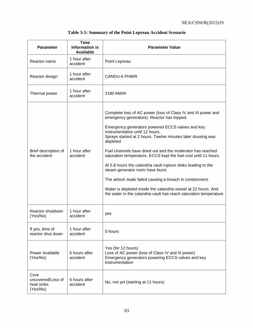
NEA/CSNI/R(2015)19
63
Table 3-5: Summary of the Point Lepreau Accident Scenario
Parameter Time
Information is Available
Parameter Value
Reactor name 1 hour after accident
Point Lepreau
Reactor design 1 hour after accident
CANDU-6 PHWR
Thermal power 1 hour after accident
2180 MWth
Brief description of the accident
1 hour after accident
Complete loss of AC power (loss of Class IV and III power and emergency generators). Reactor has tripped. Emergency generators powered ECCS valves and key instrumentation until 12 hours. Sprays started at 2 hours. Twelve minutes later dousing was depleted Fuel channels have dried out and the moderator has reached saturation temperature. ECCS kept the fuel cool until 11 hours. At 5.8 hours the calandria vault rupture disks leading to the steam generator room have burst. The airlock seals failed causing a breach in containment. Water is depleted inside the calandria vessel at 22 hours. And the water in the calandria vault has reach saturation temperature
Reactor shutdown (Yes/No)
1 hour after accident
yes
If yes, time of reactor shut down
1 hour after accident
0 hours
Power Available (Yes/No)
6 hours after accident
Yes (for 12 hours) Loss of AC power (loss of Class IV and III power) Emergency generators powering ECCS valves and key instrumentation
Core uncovered/Loss of heat sinks (Yes/No)
6 hours after accident
No, not yet (starting at 11 hours)

NEA/CSNI/R(2015)19
64
Parameter Time
Information is Available
Parameter Value
If yes, time the core is uncovered/heat sinks lost
6 hours after accident
Moderator reaches saturation temperature at 3.9 hours. High pressure ECCS starts at 3.9 hours, ends at 5.3 hours. Medium pressure ECCS starts at 5.3 hours, ends at 11 hours. Water is depleted inside the calandria at 22 hours.
Core temperature 6 hours after accident
1125° K
Containment pressure
1 day after accident
130 kPa(a)
Containment failed (Yes/No)
1 day after accident
Yes
If yes, time of containment failure
1 day after accident
13 hours after the accident the airlock seals failed to the atmosphere (with a hole area of 0.018554 m
2).
If no, venting status (e.g. has venting started, flow rate)
1 day after accident
No venting
3.5.2 Radionuclide Release
The first fission products are released into the heat transport system when fuel channels start to dry
out at 3.8 hours. However, the release is limited and high pressure ECCS injection prevents further
release for a time. Significant releases do not start until 15 hours, when the reactor core is disassembling
and collapsing into the calandria vessel. With containment already failed at 13 hours, radionuclides are
then released to the environment. Further releases occur after 69 hours, when CCI begins. A total of
4.11x10¹⁷
Bq of iodine is released in this scenario and 9.24x10¹⁵
Bq of caesium is released.

NEA/CSNI/R(2015)19
65
4 RESULTS OF PEACH BOTTOM SIMULATION USING FAST-RUNNING TOOLS
This section presents the assumptions the participants made in modelling the Peach Bottom accident
scenario as well as the results they obtained.
Table 4-1 indicates which organisations used their software tools to model the Peach Bottom
scenario and what datasets they modelled. Table 4-2 shows which organisations modelled the dispersion
of the source term and calculated doses and whether the dispersion codes used the source term provided
from the SOARCA report, the participant’s own source term, or both.
Table 4-1: Participants Estimating Source Terms for the Peach Bottom Scenario
Organisation Code Used Datasets Used
1 hour 6 hours 24 hours
ABmerit ESTE √
Areva MC_Transport √
CNSC RASCAL 4.3 √ √ √
IRSN PERSAN √
JRC MAAP 4.0.8 √ √
USNRC RASCAL 4.3.1 √ √ √
Table 4-2: Participants Estimating Doses for the Peach Bottom Scenario
Organisation Code Used Source Term(s) Used
ABmerit ESTE ESTE,
SOARCA
CNSC RASCAL 4.3 RASCAL,
SOARCA
IRSN C3X PERSAN
SOARCA
KIT RODOS SOARCA
NPCIL ACTREL SOARCA
University of Stuttgart ABR MC_Transport,
SOARCA
USNRC RASCAL 4.3.1 RASCAL
4.1 Assumptions in Modelling the Peach Bottom Scenario
4.1.1 Accident Progression and End State
An important assumption made by participants who modelled all datasets was the end state of each
accident scenario, based on limited information in each dataset. Several participants, such as the CNSC

NEA/CSNI/R(2015)19
66
and the JRC, assumed all scenarios would progress to a severe accident with major radionuclide releases,
including early datasets that did not indicate future containment failures. In comparison, the USNRC
analyses were based on information provided in each dataset, and did not make accident progression
assumptions that were not supported by the data, in accordance with the study objectives. Therefore, for
the 1-hour and 6-hour datasets, containment was assumed to be intact because there was no indication of
future containment failure at that time. It is important to note that the USNRC’s modelling of each 1-hour
and 6-hour dataset was done assuming no failures beyond what was explicitly stated in the dataset,
whereas other participants assumed future failures even during the early stages of an accident. For the 24-
hour datasets, the USNRC’s analyses show that if future degradation of the reactor is assumed in the
analysis, the predicted source terms change significantly. The 24-hour dataset provided all information
available to study participants on the accident scenario.
It was noted that differences in forecasting accident progression with limited data by the study
participants resulted in source term estimates that varied by orders of magnitude for the 1-hour and 6-hour
datasets. However, source term estimates for the 24-hour dataset indicated less variability because all
participants used similar assumptions regarding the end state of the accident scenario.
4.1.2 Use of SOARCA Data for Source Term Comparisons
The Peach Bottom scenario was taken from NUREG/CR-7110, Volume 1 Revision 1, entitled
“State-of-the-Art Reactor Consequence Analyses Project, Volume 1: Peach Bottom Integrated Analysis,”
(hereafter referred to as the “Peach Bottom Report”) [11-2]. The Peach Bottom report contains a complete
analysis of the scenario and the participants made use of that analysis to varying amounts [11-2].
The CNSC assumed that in the case of a real event, a complete, detailed description would not be
available due to the inherent unpredictability of severe accidents. Therefore, when performing analyses
for the Peach Bottom scenario, the CNSC assumed that the detailed analyses of the scenarios in Peach
Bottom report (i.e., section 5) were unavailable. The information presented in section 3 of the Peach
Bottom report on the initial conditions of the accident was used, as this information is equivalent to the
information that was provided to the participants. With the assumption that in-depth analyses of Peach
Bottom were unavailable, the CNSC turned to Fukushima for guidance on accident progression in a BWR
during an unmitigated station blackout.
The JRC also did not use the accident description in the Peach Bottom report after the first hour
when analysing the 1-hour dataset and when analysing the later datasets, only used information on
operator actions. Based on the initiating event and the subsequent operator actions, MAAP4 estimates the
accident progression and consequences. As all the operator actions occur between one and six hours, the
analysis of the 6-hour and 24-hour datasets were considered identical
The USNRC calculations for the 1-hour scenario and for the 6-hour scenario did not assume a severe
accident progression based on information available in the 1-hour and 6-hour datasets. USNRC used
insights from the SOARCA analyses to confirm the time of core uncovery and the start of radionuclide
releases from the core to containment and environment. The USNRC used additional data from the Peach
Bottom report when analysing the 24-hour dataset. The core release fractions documented in Figure 5-10
of the Peach Bottom report [11-2] are incorporated into RASCAL to determine the release to
containment. The Peach Bottom report was then used to verify the containment volume in RASCAL and
to determine that fission products escaped to the atmosphere through the wetwell and drywell. Finally, the
USNRC used containment pressure measurements and an equivalent hole size in containment to
determine the rate of releases to the environment. The equivalent hole sizes and pressure measurements
inputted into RASCAL were adjusted to match the pressure curve in the Peach Bottom Report (Figure 5-
8) [11-2].

NEA/CSNI/R(2015)19
67
4.1.3 Initial Core Inventory
RASCAL contains a default core inventory for Peach Bottom, and the ESTE analyses in this study
took into account specific plant parameter values for Peach Bottom. RASCAL and ESTE also provide
default core inventories for a generic BWR that are based on SCALE/ORIGEN calculations. Areva used
the initial fission product inventory of Krümmel, a German BWR, for their Peach Bottom analysis.
Fission product inventories were adjusted as necessary. The CNSC scaled the RASCAL inventories by
multiplying them by the ratio of Peach Bottom’s thermal power (3514 MW) to the RASCAL default
power (3951 MWth). Areva used the same approach with MC_Transport, except that the inventories were
multiplied by the ratio of Peach Bottom’s electric power to that of Krümmel. The pre-calculated inventory
for ESTE was done for 3514 MWth, so it did not need to be adjusted.
The USNRC adjusted the Peach Bottom inventory as follows. The reactor power was reduced to
3514 MWth to match the reactor power specified in Table 4-1 of the Peach Bottom Report [11-2].
Appendix A of the Peach Bottom Report states that the analysis is based on mid-cycle fuel, with a lead-
assembly burnup of 49 MWd/kg. It was assumed that the lead assembly burnup is larger than the batch
average burnup, fuel is in the reactor for three cycles, the burnup rate is linear within each cycle, and the
mid-cycle core-average burnup is about 29 GWd/MTU. This burnup value is about the same as the
RASCAL default burnup value of 30,000 MWd/MTU (30 GWd/MTU). The RASCAL default burnup
value was used for the calculations. It is considered conservative for the purpose of estimating
radionuclide releases from the reactor core.
The initial fission product inventories in MAAP4 Peach Bottom model are defined in the parameter
file; however they are defined as the initial masses of 25 elements. JRC used the fission product
inventories defined in Appendix A of the Peach Bottom report as the initial fission product inventories,
since most of the radionuclides are considered in MAAP4 [11-2].
4.1.4 Core Cooling
In section 3 of the Peach Bottom report it is stated that DC power is available from batteries for four
hours [11-2]. The station blackout model in RASCAL 4.3 assumes that it takes six hours after cooling is
lost for the fuel to be uncovered, so the CNSC and USNRC assumed that the core became uncovered ten
hours into the accident scenario when analysing the 1-hour dataset. The 6-hour dataset indicated that the
core was uncovered at 8.4 hours. Because the six-hour timing between loss of cooling and the core being
uncovered cannot be changed in RASCAL, the CNSC and USNRC reduced the time before cooling was
lost to 2.4 hours (even though the dataset indicates that cooling is available for four hours).
As the JRC did not use the accident progression detailed in the Peach Bottom report when analysing
the 1-hour dataset, certain aspects of the accident progression were not included in their MAAP4 analysis
of the 1-hour dataset. For example, a stuck open safety relief valve at eight hours into the accident
scenario, and operator control of the RCIC two hours into the accident scenario. For their analysis of the
24-hour dataset, JRC included these events. Since the MAAP4 logic requires RCIC to be stopped once
DC power is exhausted. As a result, MAAP4 shut it off 1.2 hours early.
4.1.5 Release Path
The CNSC and USNRC assumed different release pathways to the atmosphere when using
RASCAL. RASCAL version 4.3 allows the selection of either the wetwell or drywell (but not both) as a
release path for a BWR. The CNSC assumed a release through the drywell wall for all three datasets
because it used the events at Fukushima Daiichi Unit 1 as a guide for severe accident progression in a
BWR [11-4]. However, the USNRC assumed that the release went through the wetwell (suppression

NEA/CSNI/R(2015)19
68
pool), that was saturated. Even for the 24-hour dataset, when the drywell liner was assumed to be melted
through, the USNRC selected a release through the wetwell because some of the release still travelled
through the wetwell and RASCAL models the wetwell and drywell with a shared containment volume.
ABmerit also assumed that the release was initially through the suppression pool, which was assumed to
be subcooled until 10 hours into the accident. After drywell melt-through occurs at 19 hours into the
accident, ABmerit assumed all releases then bypassed the wet well.
Prior to containment failure, releases to the environment were due to containment leakage. ABmerit
assumed that leakage was equivalent to a release of 1% of the containment volume per day, while the
CNSC used the design leak rate for Peach Bottom built into RASCAL. RASCAL will also calculate
release rates based on pressure in containment and the size of hole in containment. USNRC used data
from the SOARCA report to generate containment pressures for the scenario and then used data from a
standard RASCAL output file to check containment pressures calculated by RASCAL with the SOARCA
data. The SOARCA data, plus assuming an initial hole size with an equivalent area of 0.13 cm2, was their
method of modelling leakage.
Containment fails 20 hours into the Peach Bottom scenario. To capture containment failure in ESTE,
ABmerit increased the release rate from 1% per day to 200% per day. The CNSC modelled containment
failure as a release rate of 50% per hour for the first hour after containment failure followed by a release
rate 1% per hour from then on. This was based on NUREG-1940, where the same approach was applied
when using RASCAL to model Fukushima units 1 and 3 [11-5].
Due to the drywell melt-through and pressure rising in containment, the USNRC increased the size
of the hole in containment to 0.01 m2 at 19.5 hours, 0.1 m
2 at 19.75 hours, before finally reaching a
maximum size of 1 m2 when containment fails at 20 hours. The CNSC also used the containment pressure
and hole size feature in RASCAL to model containment failure for the 24-hour dataset. Pressure in
containment at the time of containment failure was known from the dataset and a hole of 15.4 cm in
diameter was assumed to represent the containment breach (the size comes from the size of containment
failures in analyses of CANDU reactors). It should be noted that the USNRC and CNSC terminated the
RASCAL calculations at different times and this has a direct effect on the release timing and location.
4.2 Peach Bottom Results
This section presents comparisons of the source term estimates for the Peach Bottom scenario. Table
4-3 has the values and Figures 4-1 to 4-3 graphically compare the source term estimates.

NEA/CSNI/R(2015)19
69
Table 4-3: Source Term Estimates of Peach Bottom Scenario (TBq)
Organisation CNSC ABmerit Areva JRC USNRC IRSN
Software Tool RASCAL 4.3 ESTE MC_Transport MAAP4 4.0.8 RASCAL
4.3.1 PERSAN
Dataset 1hr 6hrs 24hrs 24hrs 24hrs 1hr 24hrs 24hrs 24hrs
Radionuclides
Noble Gases
Kr-85 2.20E+04 2.10E+04 8.30E+03 4.31E+04 1.11E+06 3.74E+04 3.74E+04 2.80E+04 1.88E+04
Kr-85m 8.40E+03 8.60E+03 1.00E+04 2.01E+04 7.09E+04 5.93E+04 4.11E+04 3.72E+04 1.08E+04
Kr-87 1.50E+00 4.90E+00 1.40E+02 1.76E+01 6.38E+00 9.05E+01 2.40E+01 3.40E+01 1.69E+02
Kr-88 2.50E+03 2.70E+03 7.50E+03 7.60E+03 1.30E+04 3.10E+04 1.73E+04 1.71E+04 6.62E+03
Xe-133 3.60E+06 3.50E+06 1.40E+06 5.84E+06 4.91E+06 7.06E+06 7.07E+06 6.34E+06 5.11E+06
Xe-133m 9.10E+04 8.80E+04 3.60E+04 1.67E+05 1.38E+05 1.72E+05 6.32E+05
Xe-135 5.70E+05 5.40E+05 3.30E+05 1.38E+06 9.26E+05 7.18E+05 6.10E+05 1.36E+06 3.25E+04
Total Noble Gases 4.33E+06 4.19E+06 1.81E+06 7.57E+06 7.23E+06 7.91E+06 7.78E+06 8.01E+06 5.98E+06
Iodine
I-131 1.60E+05 1.40E+05 1.10E+05 4.01E+04 9.23E+04 2.27E+06 8.11E+04 9.35E+04 3.28E+05
I-132 1.70E+05 2.00E+05 1.50E+05 3.71E+04 1.45E+05 8.33E+03 1.34E+02 1.22E+05 3.79E+05
I-133 1.50E+05 1.30E+05 1.30E+05 3.21E+04 1.11E+05 2.77E+06 9.26E+04 1.04E+05 2.46E+05
I-135 2.40E+04 2.20E+04 4.00E+04 6.55E+03 1.88E+04 7.27E+05 2.06E+04 2.38E+04 3.89E+04
Total Iodine 5.04E+05 4.92E+05 4.30E+05 1.16E+05 3.67E+05 5.78E+06 1.94E+05 3.43E+05 9.92E+05
Alkali Metals
Cs-134 2.50E+04 2.20E+04 1.30E+04 6.14E+03 3.95E+03 1.14E+05 5.46E+04 3.84E+03 8.71E+03
Cs-136 7.50E+03 6.40E+03 3.90E+03 1.87E+03 8.23E+02 4.33E+04 2.07E+04 1.50E+03 5.34E+03
Cs-137* 1.70E+04 1.50E+04 8.90E+03 5.24E+03 3.09E+03 1.18E+05 5.66E+04 2.66E+03 8.59E+03

NEA/CSNI/R(2015)19
70
Organisation CNSC ABmerit Areva JRC USNRC IRSN
Software Tool RASCAL 4.3 ESTE MC_Transport MAAP4 4.0.8 RASCAL
4.3.1 PERSAN
Dataset 1hr 6hrs 24hrs 24hrs 24hrs 1hr 24hrs 24hrs 24hrs
Total Caesium 4.95E+04 4.34E+04 2.58E+04 1.32E+04 7.86E+03 2.75E+05 1.32E+05 8.00E+03 2.26E+04
Total Tellurium 2.94E+05 2.55E+05 1.85E+05 5.08E+04 2.10E+05 2.42E+06 1.10E+06 4.60E+04 1.27E+05
Total Strontium 3.38E+04 3.39E+04 1.17E+04 1.97E+04 9.69E+05 6.39E+02 1.36E+02 2.03E+03
Total Ruthenium 5.56E+03 4.45E+03 3.96E+03 7.25E+02 2.02E+03 4.72E+01 4.25E+00 3.86E+03
Additional Radionuclides
Ba-140 4.80E+04 4.60E+04 1.60E+04 1.66E+04 2.81E+03
La-140 4.00E+03 4.10E+03 1.10E+03 8.80E+02 2.81E+00 2.16E+02
Mo-99 5.00E+04 4.30E+04 2.70E+04 5.40E+02 1.16E+04
Nb-95 1.70E-09 1.21E+03 5.20E+00
Np-239 3.70E+04 3.80E+04 1.10E+04 6.40E+03 4.75E+01
Rb-88 2.60E+03 2.70E+03 6.40E+03 2.97E+02 2.62E+03
Tc-99m 4.60E+04 4.10E+04 2.60E+04 5.17E+02 1.11E+04
Other additional radionuclides
4.25E+04 4.07E+04 1.92E+04 9.43E+03 3.65E+01 8.01E+03
Total Additional Radionuclides
2.30E+05 2.16E+05 1.07E+05 3.59E+04 3.93E+01 3.64E+04
Total 5.44E+06 5.23E+06 2.58E+06 7.80E+06 8.79E+06 1.64E+07 9.20E+06 8.45E+06 7.12E+06
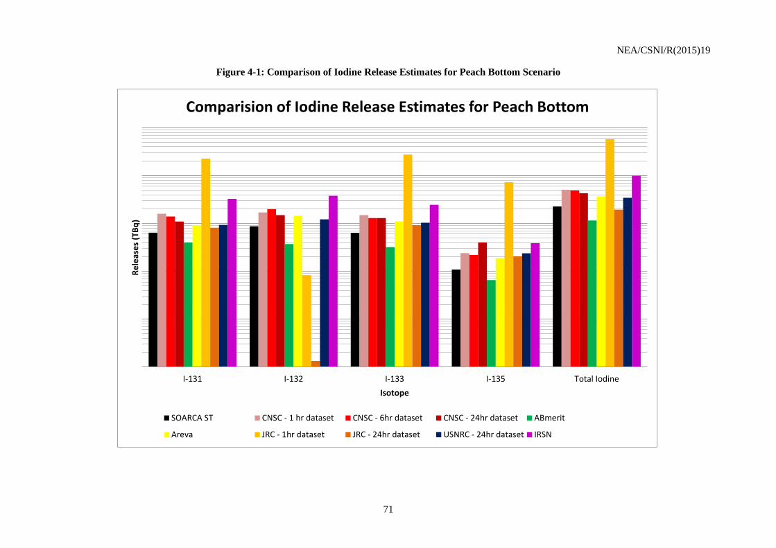
NEA/CSNI/R(2015)19
71
Figure 4-1: Comparison of Iodine Release Estimates for Peach Bottom Scenario
I-131 I-132 I-133 I-135 Total Iodine
Re
leas
es
(TB
q)
Isotope
Comparision of Iodine Release Estimates for Peach Bottom
SOARCA ST CNSC - 1 hr dataset CNSC - 6hr dataset CNSC - 24hr dataset ABmerit
Areva JRC - 1hr dataset JRC - 24hr dataset USNRC - 24hr dataset IRSN

NEA/CSNI/R(2015)19
72
Figure 4-2: Comparison of Caesium Release Estimates for Peach Bottom Scenario
Cs-134 Cs-136 Cs-137* Total Caesium
Re
leas
es
(TB
q)
Isotopes of Cs
Comparison of Cs Release Estimates for Peach Bottom
SOARCA ST CNSC - 1hr dataset CNSC - 6hr dataset CNSC - 24hr dataset ABmerit
Areva JRC - 1hr dataset JRC - 24hr dataset USNRC - 24hr dataset IRSN

NEA/CSNI/R(2015)19
73
Figure 4-3: Comparison of Noble Gas and Total Release Estimates for Peach Bottom Scenario
Xe-133 Total Noble Gases Total
Re
leas
es
(TB
q)
Comparison of Noble Gas and Total Release Estimates for Peach Bottom
SOARCA ST CNSC - 1hr dataset CNSC - 6hr dataset CNSC - 24hr dataset ABmerit
Areva JRC - 1hr dataset JRC - 24hr dataset USNRC - 24hr dataset IRSN

NEA/CSNI/R(2015)19
74

NEA/CSNI/R(2015)19
75
5 RESULTS OF SURRY SIMULATION USING FAST-RUNNING TOOLS
This section presents the assumptions the participants made in modelling the Surry accident scenario as
well as the results they obtained.
Table 5-1 indicates which organisations used their software tools to model the Surry scenario and
what datasets they modelled. Table 5-2 shows which organisations modelled the dispersion of the source
term and calculated doses and whether the dispersion codes used the source term provided from the
SOARCA report, the participant’s own source term, or both.
Table 5-1: Participants Estimating Source Terms for the Surry Scenario
Organisation Code Used Datasets Used
1 hour 6 hours 24 hours
ABmerit ESTE √
Areva MC_Transport √
CNSC RASCAL 4.3 √ √ √
IRSN PERSAN √
MER √
JRC MAAP 4.0.8 √ √
KAERI SURSOR √ √ √
USNRC RASCAL 4.3.1 √ √
Table 5-2: Participants Estimating Doses for the Surry Scenario
Organisation Code Used Source Term(s) Used
ABmerit ESTE ESTE, SOARCA
CNSC RASCAL 4.3 RASCAL, SOARCA
IRSN C3X PERSAN, MER, SOARCA
KAERI MACCS2 SURSOR
KIT RODOS SOARCA
NPCIL ACTREL SOARCA
University of Stuttgart ABR MC_Transport,
SOARCA
USNRC RASCAL 4.3.1 RASCAL
5.1 Assumptions in Modelling the Surry Scenario
5.1.1 Accident Progression and End State
As discussed in previous sections, one of the most important assumptions that participants had to
make in this study concerned the end state of the accident scenario based on limited information in the

NEA/CSNI/R(2015)19
76
datasets. Consistent with the Peach Bottom analyses, several participants assumed that each scenario
would progress to a severe accident involving major radionuclide releases, due to containment failure and
other severe-accident modelling assumptions. In comparison, the USNRC and KAERI did not make
assumptions about the end state of the accident that were not based on information contained in the
datasets. Accordingly, they assumed that containment remained intact when modelling the early datasets.
Also, for the Surry 1-hour dataset, the USNRC did not perform an analysis because the limited
information on plant conditions did not indicate a major accident in the future. KAERI assumed that
containment remained intact, even when analysing the Surry 24-hour dataset, because containment breach
does not occur until 45 hours into the accident scenario (KAERI did run a fourth analysis with all the
information).
Similar to the Peach Bottom analyses, these different approaches in modelling the accident scenarios
resulted in source term estimates that differ by orders of magnitude. KAERI’s modelling of all Surry
datasets and the USNRC’s modelling of 6-hour datasets did not assume a severe accident or containment
failure because there was no indication of future containment failure in the dataset. Thus, the USNRC’s
modelling of all the and 6-hour datasets assumed no failures beyond what was explicitly stated in the
dataset, whereas several participants assumed future failures even in the early stages of the accident with
limited data. Analyses of the USNRC’s 24-hour dataset shows that predicted source terms change
significantly and are consistent with source terms predicted by participants that assumed initially that
scenario progressed to a severe accident based on limited data.
5.1.2 Use of SOARCA Data for Source Term Comparisons
The Surry scenario was taken from NUREG/CR-7110, Volume 2 Revision 1, entitled “State-of-the-
Art Reactor Consequence Analyses Project, Volume 2: Surry Integrated Analysis,” (hereafter referred to
as the “Surry Report”) [11-3]. The Surry report contains a complete analysis of the scenario and
information on source terms, which the participants used in their analyses to varying degrees.
The CNSC again assumed that in the case of a real event, a complete, detailed description would not
be available due to the inherent unpredictability of severe accidents. And so the CNSC assumed that the
detailed analyses of the scenarios in Surry report (i.e., section 5) were unavailable, while the information
presented in section 3 of the Surry report on the initial conditions of the accident was available. Also,
unlike the Peach Bottom scenario where Fukushima could be used for reference, there has never been a
severe accident at a PWR caused by a station blackout. The CNSC used analyses of station blackouts at
Point Lepreau for guidance on accident progression as both Point Lepreau and Surry have large, dry
containments. To account for the different core design the following assumption was made: that fuel
channels drying out in a CANDU core is equivalent to the core becoming uncovered in a LWR.
The JRC also did not use the accident description in the Surry report after the first hour when
analysing the 1-hour dataset and when analysing the later datasets, and only used information on operator
actions and systems availability. Again all the operator actions occur between one and six hours, the
analysis of the 6-hour and 24-hour datasets are identical. However, the Surry report was used to adjust the
MAAP4 model of the JRC PWR 3 loops plant. A TD-AFW system was incorporated into the MAAP4
parameter file and mass flow through the steam generator relief and safety valves was added to the model.
When analysing the 6-hour dataset, the USNRC used the SOARCA data to determine when core
cooling would be lost from the TD-AFW due to load off control power when the DC batteries were
exhausted. Then, when analysing the 24-hour dataset, the USNRC again used the Surry report to
determine accident progression timing and phenomena and incorporated them into RASCAL. The report
was used to verify the containment volume in RASCAL and to determine that the release was through
containment, rather than bypassing it. Finally, as with the Peach Bottom scenario, the USNRC used

NEA/CSNI/R(2015)19
77
containment pressure measurements and an equivalent hole size in containment to determine the rate of
releases to the environment. The equivalent hole sizes and pressure measurements inputted into RASCAL
were adjusted to match the pressure curve in the Surry Report (Figure 5-8) [11-3].
5.1.3 Initial Core Inventory
RASCAL and ESTE contain default core inventories of fission products for a generic PWR; both
based on SCALE/ORIGEN calculations. In ESTE’s case they were specifically calculated for Surry.
RASCAL adjusts the initial core inventory based on power and estimated burnup. Areva used the power-
adjusted initial fission product inventory of a generic German 4-loop PWR for their Surry analysis. The
initial fission product inventories in the MAAP4 JRC PWR 3 loops model are defined in a parameter file;
however they are defined as the initial masses of 25 elements. JRC used the fission product inventories
defined in Appendix B of the Surry report as the initial fission product inventories, since most of the
radionuclides are considered in MAAP4 (initial activity in Curies) [11-3].
The USNRC adjusted the default core inventory in RASCAL for Surry as follows. The reactor
power was reduced to 2546 MWth to match the power specified in Table 4-1 of the Surry Report. Section
4.3 of that report states that the Surry decay heat is based on a lead-assembly burnup of 59 GWd/MTU,
which is assumed to be end-of-cycle burnup. Assuming the lead assembly burnup is slightly larger than
the batch average burnup, fuel is in the reactor for three cycles, and the burnup rate is linear within each
cycle, the mid-cycle core-average burnup is about 29 GWd/MTU. This burnup value is about the same as
the RASCAL default burnup value of 30,000 MWd/MTU (30 GWd/MTU). The RASCAL default value,
which is considered conservative for the purpose of estimating radionuclide releases from the reactor
core, was used for the calculations.
5.1.4 Core Cooling
When assessing the 1-hour dataset, the CNSC assumed that DC power at Surry lasted for 7.1 hours,
as that’s how long the batteries lasted in the Point Lepreau analysis used as a basis for the assessment.
The station blackout model for a PWR in RASCAL 4.3 assumes that it takes eight hours after cooling is
lost for the fuel to be uncovered, so it was assumed that the core became uncovered 15.1 hours into the
accident scenario. The 6-hour dataset states that the core will be uncovered at 14 hours, so core cooling is
assumed to last for six hours.
The NRC considered the prediction in the 6-hour dataset that the core could be uncovered in 14
hours into the accident. RASCAL default parameter values were used because the 6-hour dataset assumed
that batteries were drained after 6 hours and core cooling is lost at that time. RASCAL assumes it takes
eight hours for the core to become uncovered once cooling is lost. The time that the core is uncovered in
the NRC analysis is the same as the 14-hour estimate provided in the 6-hour dataset. The USNRC used
the accident progression timing of SOARCA for its 24-hour dataset.
KAERI also ignored the predicted timing of core uncovery. For their analyses of the 1-hour and 6-
hour datasets, inputs into their software tool SURSOR (XSOR for Surry) were that there was no vessel
breach and that pressure in the cooling system was normal (2500 psi(a)). For the analysis of the 24-hour
dataset, these parameters were changed so that a breach had occurred and the coolant pressure was < 200
psi(a). It was also assumed at that point that most of the core was involved in CCI and that a large amount
(>65%) of the zirconium was being oxidised.
When analysing the 1-hour dataset, JRC assumed that the TD-AFW would last as long as there was
DC power, which was estimated to be eight hours. JRC also assumed that the steam generator power
operated relief valves would remain closed. The other datasets indicated that these assumptions were

NEA/CSNI/R(2015)19
78
incorrect and JRC’s analysis of the 24-hour dataset was done with the TD-AFW shut off at six hours and
the steam generator PORV opened at 1.5 hours.
5.1.5 Release Path
CNSC used the design leak rate for Surry built into RASCAL to model containment leakage. After
containment failure, the CNSC again used the guidance of NUREG-1940 in analysing the 1-hour and 6-
hour datasets, modelling containment failure as a 50% per hour release rate for one hour followed by a
1% per hour release rate [11-5]. With the 24-hour dataset, the CNSC used the RASCAL feature that
allows the release rate to be calculated as a function of containment pressure and the size of a hole in
containment. At 24 hours the CNSC used the provided pressure measurement of 248.7 kPa(g) and
assumed that containment leakage was equivalent to a hole size of one square inch. At 45 hours into the
accident, the hole size was increased to 186.3 cm2 as that was the equivalent hole size of airlock seal
failure from the Point Lepreau analysis being used as a baseline. Containment pressure at that time was
assumed to be 1 MPa(g).
In the Point Lepreau analysis the CNSC used to estimate accident progression for the Surry scenario,
airlock seals fail approximately six hours after the fuel channels dry out. This timing had to be adjusted
though, because while Point Lepreau and Surry have similar containment designs, the reactor power, the
amount of water in the core and the containment volume all differ. It was assumed that time of
containment failure is directly proportional to these variables, so the six hour estimate from the Point
Lepreau analysis was adjusted based on these parameters. While Surry has a greater containment volume
and less water in the core that can be converted to steam, its higher power could lead to faster
pressurisation. In the end it was estimated that containment would fail five hours after the core was
uncovered. However, the 24-hour dataset showed that this assumption was quite a bit off as containment
does not fail until 31 hours after the core is uncovered.
Like with Peach Bottom, NRC used data from the SOARCA report to generate containment
pressures for the scenario and then used data from a standard RASCAL output file to check containment
pressures calculated by RASCAL with the SOARCA data. This data was used along with estimating a
hole size to model the release rates in RASCAL. At first, the hole was assumed to be 0.08 cm2. At the
onset of containment failure (45.5 hours), it was increased to 5.3 cm2. Over the next 11.5 hours, the hole
in containment was assumed to grow to 33.7 cm2 and 63 hours into the accident, it was assumed to be
37.2 cm2.
To ensure that MAAP4 captured releases due to leakage, JRC added a leak pathway from the upper
part of containment to the environment to the JRC PWR 3 Loops model. Areva modelled containment
leakage as 0.5% of the containment volume released per day and ABmerit modelled leakage as 1%
released per day. ABmerit increased this to 400% per day once containment failed. KAERI model
containment failure by assuming that it developed from an existing leak point and that the size of the
breach is approximately 93 cm2 (0.1 square feet).
5.2 Surry Results
This section presents comparisons of the source term estimates for the Surry scenario. Table 5-3 has
the values and Figures 5-1 to 5-3 graphically compare the source term estimates.
Also note that the SURSOR results (both source term and doses) list results for 24 hours and all data.
The 24 hour data refers to the information that would be explicitly available after 24 hours, which is not
the same as the information available in the 24-hour dataset. As containment does not fail until 24 hours,

NEA/CSNI/R(2015)19
79
this would not be explicitly known at that time. The results categorised as “All Data” are the results
produced by SURSOR using all the data that was available.

NEA/CSNI/R(2015)19
80
Table 5-3: Analysis Results of Surry Scenario (TBq)
Organisation CNSC
ABmerit Areva JRC KAERI USNRC
IRSN
Software Tool RASCAL 4.3 ESTE
MC_Transport MAAP4 4.0.8 SURSOR
RASCAL 4.3.1
PERSAN MER
Dataset 1hr 6hr 24hr 24hr 24hr 1hr 24hr 24hr* All Data 24hr 24hr 24hr
Radionuclides
Noble Gases
Kr-85 1.00E+0
4 1.00E+0
4 6.80E+0
3 2.0E+04 2.50E+04
2.79E+04
2.85E+04
8.73E+0
3 1.79E+0
4 2.05E+0
4
Kr-85m 2.50E+0
3 3.00E+0
3 9.00E+0
2 4.7E+02 4.77E+02
2.69E+03
2.83E+03
4.40E+0
1 5.27E+0
2 6.00E+0
2
Kr-87 1.10E+0
0 2.00E+0
0 1.10E+0
0 1.1E-01 2.10E+01
7.92E-03
6.69E-03
3.41E-
03 9.35E-
02 1.53E+0
0
Kr-88 8.40E+0
2 1.10E+0
3 3.80E+0
2 6.3E+01 1.61E+02
3.14E+02
3.18E+02
3.28E+0
0 7.32E+0
1 1.30E+0
2
Xe-133 1.70E+0
6 1.70E+0
6 1.00E+0
6 3.4E+06 4.44E+06
5.82E+06
5.95E+06
2.82E+0
6 1.59E+0
6 4.73E+0
6 4.25E+0
6
Xe-135 2.20E+0
5 2.40E+0
5 7.90E+0
4 2.4E+05 2.94E+05
1.28E+05
1.36E+05
3.37E+0
4 2.37E+0
5 2.49E+0
5
Xe-135m 4.10E+0
3 4.60E+0
3 1.60E+0
3 4.9E+03 5.57E+03
2.89E-33
1.03E-33
1.84E+0
1 4.67E+0
3 5.15E+0
3
Total Noble Gases 1.99E+0
6 2.01E+0
6 1.12E+0
6 3.78E+0
6 4.90E+06
5.98E+06
6.12E+06
3.19E+04
6.38E+06
1.68E+06
5.14E+06
4.66E+06
Iodine
I-131 1.20E+0
5 1.20E+0
5 3.60E+0
4 2.5E+03 2.15E+05
2.26E+03
3.36E+03
8.15E+0
1 8.53E+0
3 1.16E+0
4 1.21E+0
4
I-132 1.50E+0
5 1.50E+0
5 4.40E+0
4 2.9E+03 2.50E+05
7.41E-02
9.82E-02
1.19E+0
2 8.18E+0
3 1.22E+0
4 1.30E+0
4
I-133 1.10E+0 1.20E+0 3.50E+0 1.5E+03 1.11E+05 1.53E+0 2.32E+0 1.69E+0 3.09E+0 4.90E+0 5.73E+0
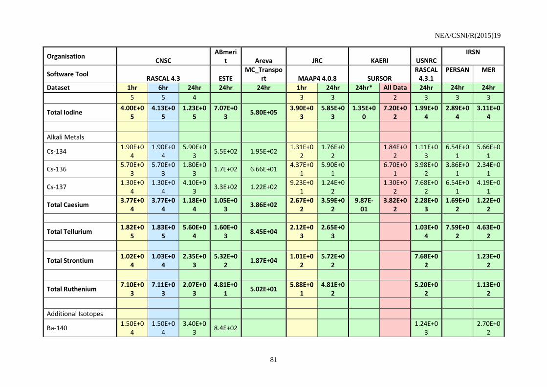
NEA/CSNI/R(2015)19
81
Organisation CNSC
ABmerit Areva JRC KAERI USNRC
IRSN
Software Tool RASCAL 4.3 ESTE
MC_Transport MAAP4 4.0.8 SURSOR
RASCAL 4.3.1
PERSAN MER
Dataset 1hr 6hr 24hr 24hr 24hr 1hr 24hr 24hr* All Data 24hr 24hr 24hr
5 5 4 3 3 2 3 3 3
Total Iodine 4.00E+0
5 4.13E+0
5 1.23E+0
5 7.07E+0
3 5.80E+05
3.90E+03
5.85E+03
1.35E+00
7.20E+02
1.99E+04
2.89E+04
3.11E+04
Alkali Metals
Cs-134 1.90E+0
4 1.90E+0
4 5.90E+0
3 5.5E+02 1.95E+02
1.31E+02
1.76E+02
1.84E+0
2 1.11E+0
3 6.54E+0
1 5.66E+0
1
Cs-136 5.70E+0
3 5.70E+0
3 1.80E+0
3 1.7E+02 6.66E+01
4.37E+01
5.90E+01
6.70E+0
1 3.98E+0
2 3.86E+0
1 2.34E+0
1
Cs-137 1.30E+0
4 1.30E+0
4 4.10E+0
3 3.3E+02 1.22E+02
9.23E+01
1.24E+02
1.30E+0
2 7.68E+0
2 6.54E+0
1 4.19E+0
1
Total Caesium 3.77E+0
4 3.77E+0
4 1.18E+0
4 1.05E+0
3 3.86E+02
2.67E+02
3.59E+02
9.87E-01
3.82E+02
2.28E+03
1.69E+02
1.22E+02
Total Tellurium 1.82E+0
5 1.83E+0
5 5.60E+0
4 1.60E+0
3 8.45E+04
2.12E+03
2.65E+03
1.03E+0
4 7.59E+0
2 4.63E+0
2
Total Strontium 1.02E+0
4 1.03E+0
4 2.35E+0
3 5.32E+0
2 1.87E+04
1.01E+02
5.72E+02
7.68E+0
2
1.23E+02
Total Ruthenium 7.10E+0
3 7.11E+0
3 2.07E+0
3 4.81E+0
1 5.02E+01
5.88E+01
4.81E+02
5.20E+0
2
1.13E+02
Additional Isotopes
Ba-140 1.50E+0
4 1.50E+0
4 3.40E+0
3 8.4E+02
1.24E+03
2.70E+0
2

NEA/CSNI/R(2015)19
82
Organisation CNSC
ABmerit Areva JRC KAERI USNRC
IRSN
Software Tool RASCAL 4.3 ESTE
MC_Transport MAAP4 4.0.8 SURSOR
RASCAL 4.3.1
PERSAN MER
Dataset 1hr 6hr 24hr 24hr 24hr 1hr 24hr 24hr* All Data 24hr 24hr 24hr
La-140 1.60E+0
3 1.60E+0
3 5.40E+0
2 4.0E+01 1.87E+00
6.24E+02
3.89E+0
1
Mo-99 3.80E+0
4 3.90E+0
4 1.20E+0
4 2.6E+01
2.01E+03
3.65E+0
2
Nb-95 2.30E+0
2 2.30E+0
2 5.20E+0
1 3.8E+01
2.20E+01
2.27E+0
1
Np-239 5.10E+0
4 5.10E+0
4 1.10E+0
4 3.0E+02
3.13E+03
1.09E+0
2
Rb-88 8.30E+0
2 1.10E+0
3 3.70E+0
2 1.7E+00
3.28E+00
2.49E+0
0
Tc-99m 3.70E+0
4 3.70E+0
4 1.10E+0
4 2.5E+01
1.94E+03
3.59E+0
2
Other additional isotopes
3.53E+04
3.57E+04
9.33E+03
3.38E+02
9.65E+01 2.57E+0
3
2.52E+02
Total Additional Isotopes
1.79E+05
1.81E+05
4.77E+04
1.60E+03
9.84E+01 1.15E+0
4
1.42E+03
Total 2.81E+0
6 2.84E+0
6 1.36E+0
6 3.80E+0
6 5.59E+06
5.99E+06
6.13E+06
3.19E+04
6.48E+06
1.72E+06
5.17E+06
4.69E+06
* When analysing the 24-hour dataset, KAERI did not use all the information that was presented as some of it, such as time of containment failure, would not
be explicitly known then. SURSOR was later runs for a fourth time using all the information. The source term in the column labelled “All Data” reflects this
fourth run

NEA/CSNI/R(2015)19
83
Figure 5-1: Comparison of Iodine Release Estimates for Surry Scenario
I-131 I-132 I-133 Total Iodine
Re
leas
es
(TB
q)
Isotope
Comparison of Surry Radioiodine Source Term Estimates
SOARCA ST CNSC 1hr dataset CNSC - 6 hr dataset CNSC - 24hr dataset ABmerit
Areva JRC - 1hr dataset JRC - 24hr dataset USNRC - 24hr dataset IRSN - PERSAN
IRSN - MER KAERI - Limited 24hr KAERI - All Data

NEA/CSNI/R(2015)19
84
Figure 5-2: Comparison of Caesium Release Estimates for Surry Scenario
Cs-134 Cs-136 Cs-137 Total Caesium
Re
leas
es
(TB
q)
Isotope
Comparison of Cs Source Term Estimates for Surry
SOARCA ST CNSC - 1hr dataset CNSC - 6hr dataset CNSC - 24hr dataset ABmerit
Areva JRC - 1hr dataset JRC - 24hr dataset USNRC - 24hr dataset IRSN - PERSAN
IRSN - MER KAERI - Limited 24hr KAERI - All Data

NEA/CSNI/R(2015)19
85
Figure 5-3: Comparison of Noble Gas and Total Release Estimates for Surry Scenario
Xe-133 Total Noble Gases Total
Re
leas
es
(TB
q)
Noble Gas and Total Source Term Estimates for Surry
SOARCA ST CNSC - 1hr dataset CNSC - 6hr dataset CNSC - 24hr dataset ABmerit
Areva JRC - 1hr dataset JRC - 24hr dataset USNRC - 24hr dataset IRSN
IRSN - MER KAERI - Limited 24hr KAERI - All Data

NEA/CSNI/R(2015)19
86

NEA/CSNI/R(2015)19
87
6 RESULTS OF OSKARSHAMN SIMULATION USING FAST RUNNING TOOLS
This section presents the assumptions the participants made in modelling the Oskarshamn accident
scenario as well as the results they obtained.
Table 6-1 indicates which organisations used their software tools to model the Oskarshamn scenario
and what datasets they modelled. Table 6-2 shows which organisations modelled the dispersion of the
source term and calculated doses.
Table 6-1: Participants Estimating Source Terms for the Oskarshamn Scenario
Organisation Code Used Datasets Used
1 hour 6 hours 24 hours
ABmerit ESTE √
Areva MC_Transport √
CNSC RASCAL 4.2 √ √ √
IRSN PERSAN √
SSM RASTEP √
USNRC RASCAL 4.3.1 √ √
Table 6-2: Participants Estimating Doses for the Oskarshamn Scenario
Organisation Code Used Source Term(s) Used
ABmerit ESTE ESTE
CNSC RASCAL 4.2 RASCAL
IRSN C3X PERSAN
University of Stuttgart ABR MC_Transport – 1 hr release
MC_Transport – 10 hr release
USNRC RASCAL 4.3.1 RASCAL
6.1 Assumptions in Modelling the Oskarshamn Scenario
6.1.1 Accident Progression and End State
As with Peach Bottom and Surry, the CNSC assumed that severe core damage would occur for all
datasets while the USNRC did not make any assumptions about the state of the reactor that was not in the
dataset (the CNSC and the USNRC were the only organisations to model more than one dataset). Also,
based on the information in the 1-hour dataset, the USNRC determined that RASCAL did not need to be
run at that point.
The differences between the CNSC results for the 1-hour, 6-hour, and 24-hour dataset and the
USNRC results for the 6-hour and 24-hour dataset again show the effect of this assumption. However, the
NEA/CSNI/R(2015)19
88
results also show that this was by no means the only assumption to have a major effect on the calculated
source terms.
6.1.2 Reactor Specification
Unlike Peach Bottom and Surry, RASCAL does not have Oskarshamn in its database, as it’s outside
the U.S. However, RASCAL allows users to define reactors not in its database using generic BWR and
PWR reactor models. CNSC staff “built” Oskarshamn in RASCAL using a generic BWR model with
Mark III containment, as that was the containment design for American BWRs constructed at the same
time as Oskarshamn. Other design parameters (number of fuel assemblies in the core, containment
volume, coolant mass, design leak rate and burn-up) came from the IAEA’s Operating Experience
(OPEX) document [11-6]. Rather than also using the generic BWR model, the USNRC actually built
Oskarshamn into RASCAL to model it. Parameters used to build the Oskarshamn model in RASCAL
include reactor power, average fuel burn-up, containment type, containment volume, containment design
pressure and design leak rate, reactor coolant mass and the number of fuel assemblies in the core. The
reactor location, topography and surface roughness of the nearby terrain were also inputted into RASCAL
to be used for dispersion modelling. One aspect of the Oskarshamn design that was not included in the
RASCAL model was the MVSS venting system. The current RASCAL interface does not have the
capability to model external, passive vent systems. However the RASCAL interface allows the user to
import and export source terms to modify them and account for external filtration systems.
ESTE has a built-in database of every European reactor. Therefore, ABmerit had access to a readily
available model for Oskarshamn.
Areva used the Krümmel to model the Oskarshamn scenario, as had been done with the Peach
Bottom scenario. The baseline scenario selected for MC_Transport was a Level 2 analysis of a core melt
followed by venting and containment melt through. The initial fission product inventory of Krümmel was
scaled down as Oskarshamn has an electrical power of 1192 MWe, while Krümmel has an electrical
power of 1400 MWe.
6.1.3 Core Cooling
As BWRs are not used in Canada, the CNSC relied on the SOARCA Peach Bottom report to provide
guidance on accident progression in BWRs, specifically, the station blackout scenarios [11-2]. For the one
hour scenario, all that was known was that residual heat removal was lost and that there were no operator
actions. Therefore, the unmitigated, short-term station blackout scenario was used to estimate how long
before the fuel was uncovered. The 6-hour dataset provided this information and indicated that auxiliary
feedwater was available. The long term station blackout scenario with mitigation in the Peach Bottom
report was then analysed to determine how long the auxiliary feedwater would last before the core was
uncovered (as the long term station blackout credits RCIC) [11-2].
The USNRC did not run an analysis for the one hour dataset, based on the information provided, as
the limited dataset did not indicate significant plant degradation at that time or in the future. Furthermore,
given the initial accident scenario, it could not be confirmed that severe core damage would result.
Therefore, no RASCAL analysis was performed. RASCAL was run for the 6-hour and 24-hour datasets,
in which the core was predicted to be uncovered at 12.7 hours.
6.1.4 Release Path
In specifying the release pathway from containment to the environment, the CNSC assumed that
releases would pass through the wetwell, as the 6-hour dataset indicated that the wet well temperature was

NEA/CSNI/R(2015)19
89
increasing and gave no indication of dry well failure. The dataset also indicated that the wet well reached
120° C at 8.8 hours; it was assumed that this meant that the wet well was saturated rather than sub-cooled
at this time. Areva also assumed that the release path went through water, although they assumed that the
drywell was flooded. Flooding the drywell accounted for the fact that Oskarshamn has a different
containment design than Krümmel and prevented containment melt-through. The scrubbing of the release
by the water in the flooded drywell was assumed to reduce the aerosol release by a factor of 10.
ABmerit assumed an initial release through the wetwell and that the wetwell would be sub-cooled
until 14 hours into the accident scenario, giving it a reduction factor of 100. At 14 hours, it was assumed
that wetwell was saturated, changing the reduction factor to 20. Then, three hours later, it was assumed
that the wetwell was bypassed and the released went through the drywell to the venting system. The
USNRC also assumed that at first fission products would travel through a sub-cooled wetwell, until 13.8
hours into the accident. Then from 13.8 hours to 19 hours, the release pathway would be through a heated
wetwell, after which the release would be through the drywell wall. However, RASCAL only allows one
release pathway to be specified, and given that the wetwell is bypassed 19 hours into the accident, the
release path the USNRC selected was through the drywell wall. After bypassing the wetwell, the release
was then assumed to go through the Standby Gas Treatment System (SBGTS). The SBGTS filters the
release and is assumed to have the same reduction factor as the MVSS.
When the USNRC was analysing the 6-hour dataset, the release via the SBGTS was assumed to
occur at 19 hours, after reactor vessel melt-through occurs. In the 24-hour dataset, it is stated that venting
occurs at 13.8 hours. However, the wetwell was not bypassed at the time of venting and RASCAL only
allows one containment release pathway to be selected. Therefore, the release calculated by RASCAL
from 13.8 hours to 19 hours was exported to a spreadsheet, had the saturated suppression pool reduction
factor applied, and then imported back into RASCAL for atmospheric transport and dispersion. For this
time period, it was assumed that venting through the suppression pool and MVSS corresponded to a
release rate of 25% of the containment volume per hour, based on converting the mass flow rate to a
volumetric flow rate and then converting that to a containment leak rate. After 19 hours, the USNRC
modelled further releases through the MVSS at a release rate of 100% per hour.
Prior to knowing the venting mass flow rate, the CNSC used NUREG-1940 for guidance. Based on
NUREG-1940, it was assumed that venting corresponded to a release rate of 25% of the containment
volume per hour [11-5]. When the mass flow rate was provided with the 24-hour dataset, it had to be
converted into the percentage of containment volume released per hour to be inputted into RASCAL.
Based on parameters from the IAEA OPEX report [11-6], venting was estimated to correspond to a
release rate of 64.13% of the containment volume released per hour. The long term station blackout with
mitigation scenario from the Peach Bottom report was also used by the CNSC to estimate when venting
would be required. The timing of the venting was adjusted based on the different containment sizes
between Peach Bottom and Oskarshamn. The 24-hour dataset indicated when venting would occur.
Areva assumed that Oskarshamn, like other BWRs, has a containment leak purging system, and as a
result, no releases due to leakage were calculated. With no containment melt-through and no leakage, the
only release Areva calculated came from the filtered venting at 14 hours, which was assumed to last for
an hour. The filter efficiencies assumed by MC_Transport were 99.9% for aerosols and 50% for
elemental iodine; noble gases were not affected by the filters and the amount of organic iodides was
assumed to be negligible. Like the USNRC, ABmerit assumed that venting corresponded to a release rate
of 100% per hour (2400% per day), and that the filter efficiency was 99.8% for iodine and aerosols.

NEA/CSNI/R(2015)19
90
6.2 Oskarshamn Results
This section presents comparisons of the source term estimates for the Oskarshamn scenario. Table
6-3 has the values and Figures 6-1 and 6-2 graphically compare the source term estimates.

NEA/CSNI/R(2015)19
91
Table 6-3: Comparison of Oskarshamn Source Term Estimates (TBq)
Organisation SSM CNSC ABmerit Areva USNRC IRSN
Software Tool RASTEP RASCAL 4.3 ESTE MC_Transport RASCAL
4.3.1 PERSAN
Dataset 24hr 1hr 6hr 24hr 24hr 24hr 24hr 24hr
Radionuclides
Noble Gases
Kr-85 3.20E+04 3.20E+04 1.40E+04 4.0E+04 3.36E+04 4.68E+04 8.42E+03
Kr-85m 1.60E+04 1.60E+04 4.20E+04 8.7E+04 1.51E+04 6.89E+04 5.12E+03
Kr-87 1.30E+01 5.10E+00 3.30E+02 4.2E+02 2.26E+00 3.08E+02 1.16E+02
Kr-88 5.70E+03 5.40E+03 3.20E+04 5.7E+04 4.17E+03 4.45E+04 3.86E+03
Xe-133 7.30E+06 6.40E+06 6.40E+06 3.10E+06 7.6E+06 4.06E+06 7.16E+06 2.26E+06
Xe-135 1.20E+06 1.30E+06 1.20E+06 2.7E+06 1.10E+06 2.67E+06 2.51E+05
Xe-135m 5.10E+04 5.80E+03 1.10E+05 2.4E+05 5.33E+04 6.62E+05 1.39E+04
Total Noble Gases 7.30E+06 7.91E+06 7.97E+06 4.61E+06 1.10E+07 5.40E+06 1.09E+07 2.62E+06
Iodine
I-131 8.82E+02 1.60E+01 2.00E+02 2.20E+02 1.4E+03 2.21E+02 3.17E+03 7.87E+04
I-132 1.40E+01 1.60E+02 2.60E+02 1.7E+03 3.52E+02 3.95E+03 8.34E+04
I-133 1.50E+01 2.00E+02 2.80E+02 1.5E+03 2.78E+02 3.55E+03 3.87E+04
Total Iodine 8.82E+02 4.78E+01 5.95E+02 8.58E+02 4.91E+03 8.56E+02 1.15E+04 2.04E+05
Alkali Metals
Cs-134 2.70E+00 3.20E+01 2.80E+01 2.5E+02 1.62E+02 7.62E+02 3.64E+00
Cs-136 9.70E-01 1.20E+01 1.00E+01 7.2E+01 3.35E+01 1.98E+02 2.19E+00
Cs-137 2.03E+02 1.80E+00 2.20E+01 1.90E+01 1.9E+02 1.26E+02 5.27E+02 3.51E+00
Total Caesium 2.03E+02 5.47E+00 6.60E+01 5.70E+01 5.04E+02 3.22E+02 1.49E+03 9.34E+00

NEA/CSNI/R(2015)19
92
Organisation SSM CNSC ABmerit Areva USNRC IRSN
Software Tool RASTEP RASCAL 4.3 ESTE MC_Transport RASCAL
4.3.1 PERSAN
Dataset 24hr 1hr 6hr 24hr 24hr 24hr 24hr 24hr
Tellurium
Te-127 1.10E+00 1.10E+01 3.80E+00 9.3E+01 5.57E+01 2.29E+02 2.89E+00
Te-129m 7.30E-01 7.50E+00 2.50E+00 5.5E+01 2.52E+01 1.50E+02 2.59E+00
Te-131m 1.40E+00 1.40E+01 5.80E+00 1.3E+02 4.85E+01 3.11E+02 3.49E+00
Te-132 1.09E+03 1.40E+01 1.40E+02 5.00E+01 1.3E+03 7.55E+02 2.90E+03 4.51E+01
Total Tellurium 1.09E+03 1.82E+01 1.82E+02 6.56E+01 1.58E+03 9.23E+02 3.79E+03 5.52E+01
Additional Radionuclides
Mo-99 1.3E+01 2.10E-01 2.60E+00 3.00E+00 1.8E+01 4.00E+01
Rb-88 1.2E+01 5.70E-01 2.70E+00 1.00E+01 8.1E+00 5.49E+01
Other Additional Radionuclides 1.8E+01 1.8E+02 5.4E+01 1.4E+03 3.6E+03
Total Additional Radionuclides 2.5E+01 1.9E+01 1.9E+02 6.7E+01 1.5E+03 3.7E+03
Total Source Term 7.30E+06 7.91E+06 7.97E+06 4.61E+06 1.10E+07 5.40E+06 1.09E+07 2.82E+06

NEA/CSNI/R(2015)19
93
Figure 6-1: Comparison of Selected Radionuclide Release Estimates for Oskarshamn Scenario

NEA/CSNI/R(2015)19
94
Figure 6-2: Comparison of Xenon and Total Release Estimates for Oskarshamn Scenario

NEA/CSNI/R(2015)19
95
7 RESULTS OF GOLFECH SIMULATION USING FAST-RUNNING TOOLS
This section presents the assumptions the participants made in modelling the Golfech accident scenario as
well as the results they obtained.
Table 7-1 indicates which organisations used their software tools to model the Golfech scenario and
what datasets they modelled. Table 7-2 shows which organisations modelled the dispersion of the source
term and calculated doses.
Table 7-1: Participants Estimating Source Terms for the Golfech Scenario
Organisation Code Used Datasets Used
1 hour 6 hours 24 hours
ABmerit ESTE √
Areva MC_Transport √
CNSC RASCAL 4.2 √ √ √
GRS ASTRID √ √ √
IRSN PERSAN √
MER √
USNRC RASCAL 4.3.1 √ √ √
Table 7-2: Participants Estimating Doses for the Golfech Scenario
Organisation Code Used Source Term(s) Used
ABmerit ESTE ESTE
CNSC RASCAL 4.2 RASCAL
IRSN C3X PERSAN
MER
ASTEC
University of Stuttgart ABR MC_Transport
USNRC RASCAL 4.3.1 RASCAL
7.1 Assumptions in Modelling the Golfech Scenario
7.1.1 Accident Progression and End State
For the previous scenarios, participants made assumptions about whether or not the accident would
progress to a severe accident based on the limited data in the 1-hour and 6-hour datasets, and as a results
total source terms varied by orders of magnitude. That was not the case for the Golfech scenario. The
nature of the accident (a large break in the hot log of the reactor cooling system with loss of safety
systems) leads to the core being uncovered so quickly that all participants assumed significant core
damage occurs for all datasets.

NEA/CSNI/R(2015)19
96
7.1.2 Reactor Specification
While RASCAL users can define a PWR using a generic model, CNSC staff were unable to find all
the design parameters of the Golfech reactor in the IAEA’s OPEX documents [11-6]. Therefore, an
American reactor, Seabrook, was chosen as a surrogate. Seabrook was selected because it is a 4 loop
PWR, like Golfech, and came online less than a year before Golfech. Seabrook does have slightly lower
power rating and peak rod burn-up than Golfech, but RASCAL allows users to adjust power and burn-up
for reactors in its database. The USNRC was able to obtain the necessary information from the IRSN to
build Golfech in RASCAL. This included the following parameters: reactor power, average fuel burn-up,
reactor coolant mass, number of fuel assemblies in the core, steam generator water mass, containment
volume, containment design pressure, and design leak rate. The reactor’s location and the surface
roughness of the nearby terrain were also used to build Golfech into RASCAL for the dispersion
calculations. For ABmerit, Golfech was also included in ESTE’s reactor database.
As with the Surry scenario, Areva used a generic PWR to model the Golfech scenario. A Level 2
PSA scenario of an 80 cm2 LOCA with injection failure at a German Konvoi reactor was used as a
baseline to model the scenario.
To model Golfech using ASTRID, GRS used ASTEC input for a generic, four loop, 1300 MWe
PWR as well as specific plant data from Konvoi type reactors. This information was used to define the
geometry of the reactor cooling system and the initial core inventory, and the ASTEC data specifically
was used to define the dimensions of containment.
7.1.3 Accident Progression
The time the core is uncovered is not included in the 1-hour dataset, so CNSC staff used a Point
Lepreau LOCA analysis to estimate when it occurs. Using the SOARCA report would have been
preferable; however, the analysis of the isolating system LOCA in the Surry Report does not indicate the
size of the break [11-3]. It was assumed that fuel channels drying out in a CANDU reactor is equivalent to
the core being uncovered in a PWR reactor. The break size in the Point Lepreau analysis was smaller than
that in the Golfech scenario, so the time for the fuel channels to dry out in the Point Lepreau scenario was
divided by the ratio of the break sizes. The final estimation was that the core was uncovered after 8
minutes; the 6-hour dataset indicated that it took 10 minutes.
In order to estimate the amount of fission products release from the fuel, and the amount that gets
retained in the coolant, GRS used validation data for the Konvoi reactor design. Calculations done for the
Konvoi reactors were also used to estimate the consequences of CCI.
7.1.4 Release Path
The CNSC used the station blackout scenarios in the Surry report to determine when containment
needed to be vented for the analyses of the 1-hour and 6-hour datasets. The release pathway selected in
RASCAL was “Containment Leakage/Failure”, even though it’s known that the release goes through a
filtered venting system. This is because for PWRs in RASCAL, filters are only available on the
“Containment Bypass” release pathway. Selecting that pathway led to extremely high doses; i.e. requiring
evacuation beyond 80 km. CNSC staff did not consider such high doses to be plausible given the accident
scenario, so the release pathway of “Containment Leakage/Failure” was selected instead. In defining the
release rate, it was assumed that the venting system at Golfech was similar to that of Point Lepreau, as the
containment design is similar. The volumetric flow rate of the Point Lepreau ventilation system was
converted into a percentage of containment that was released in an hour’s time: 16.47%. Venting was

NEA/CSNI/R(2015)19
97
assumed to last for one hour, as that was the assumption made NUREG-1940 when modelling venting at
Fukushima Unit 2 [11-5]. Leakage was assumed to be equivalent to the design leak rate of Seabrook.
USNRC used the import/export source term feature of RASCAL to effectively model external filters
because the default filter efficiency in the RASCAL user interface was not applicable to this accident
scenario and plant design. The USNRC obtained a graph from the IRSN which reported containment
pressure throughout the accident duration. Using the graph and estimates for effective hole sizes in
containment for every hour since the start of the accident, RASCAL produced an unfiltered source term at
15 minutes intervals. This source term was then exported to a spreadsheet where the filter reduction
factors were applied. It was assumed that the filters reduced particulate releases by a factor of 100, iodine
releases by a factor of 10 and did not reduce noble gas releases. The filtered source term was then
imported back into RASCAL for atmospheric transport and dispersion calculations. This approach was
only used when analysing the 24-hour dataset. It was assumed that there would not be enough time in a
real accident scenario to get the pressure measurements, develop the unfiltered source term, export it, and
apply reduction factors within six hours or less.
Areva assumed a venting rate of 25% of the containment volume released per hour, with filter
efficiencies of 99.9% for aerosol releases and 50% for elemental iodine. ABmerit assumed 1200%
released over a day (i.e. 50% per hour) with a filter efficiency of 99.8% efficiency for both iodine and
aerosol releases. Prior to venting, ABmerit assumed that containment leakage represented a release rate of
0.1% per hour. At the second FASTRUN meeting, IRSN provided GRS with information on the vent
system and filter efficiency to be modelled with ASTRID.
7.2 Golfech Results
This section presents comparisons of the source term estimates for the Golfech scenario. Table 7-3
has the values and Figures 7-1 to 7-3 graphically compare the source term estimates. It should be noted
that the list of radionuclides in Table 7-3 is not exhaustive; however, several radionuclides in the ASTEC
source term, such as I-129, Cs-134m, and radioactive bromine, was not calculate by most of the other
tools.
Note: Lacking topography data for the Golfech site, the results of the ABR calculations are presented
for the Golfech reactor located at Gravelines.
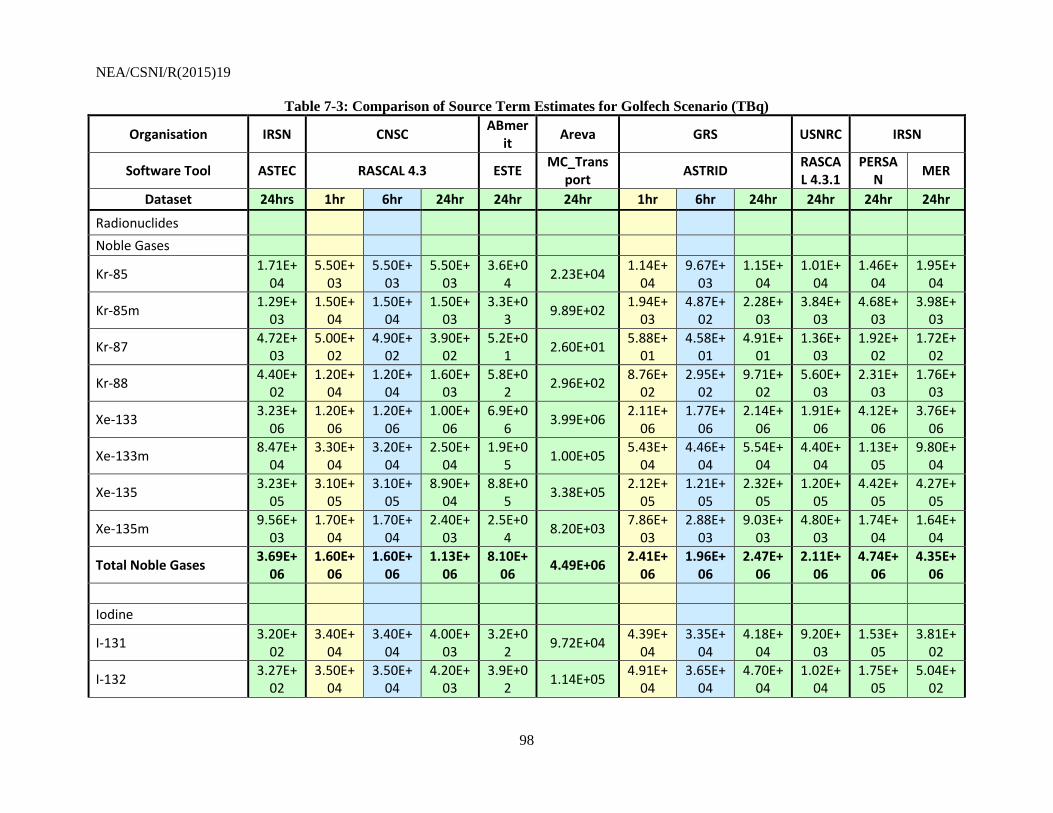
NEA/CSNI/R(2015)19
98
Table 7-3: Comparison of Source Term Estimates for Golfech Scenario (TBq)
Organisation IRSN CNSC ABmer
it Areva GRS USNRC IRSN
Software Tool ASTEC RASCAL 4.3 ESTE MC_Trans
port ASTRID
RASCAL 4.3.1
PERSAN
MER
Dataset 24hrs 1hr 6hr 24hr 24hr 24hr 1hr 6hr 24hr 24hr 24hr 24hr
Radionuclides
Noble Gases
Kr-85 1.71E+
04 5.50E+
03 5.50E+
03 5.50E+
03 3.6E+0
4 2.23E+04
1.14E+04
9.67E+03
1.15E+04
1.01E+04
1.46E+04
1.95E+04
Kr-85m 1.29E+
03 1.50E+
04 1.50E+
04 1.50E+
03 3.3E+0
3 9.89E+02
1.94E+03
4.87E+02
2.28E+03
3.84E+03
4.68E+03
3.98E+03
Kr-87 4.72E+
03 5.00E+
02 4.90E+
02 3.90E+
02 5.2E+0
1 2.60E+01
5.88E+01
4.58E+01
4.91E+01
1.36E+03
1.92E+02
1.72E+02
Kr-88 4.40E+
02 1.20E+
04 1.20E+
04 1.60E+
03 5.8E+0
2 2.96E+02
8.76E+02
2.95E+02
9.71E+02
5.60E+03
2.31E+03
1.76E+03
Xe-133 3.23E+
06 1.20E+
06 1.20E+
06 1.00E+
06 6.9E+0
6 3.99E+06
2.11E+06
1.77E+06
2.14E+06
1.91E+06
4.12E+06
3.76E+06
Xe-133m 8.47E+
04 3.30E+
04 3.20E+
04 2.50E+
04 1.9E+0
5 1.00E+05
5.43E+04
4.46E+04
5.54E+04
4.40E+04
1.13E+05
9.80E+04
Xe-135 3.23E+
05 3.10E+
05 3.10E+
05 8.90E+
04 8.8E+0
5 3.38E+05
2.12E+05
1.21E+05
2.32E+05
1.20E+05
4.42E+05
4.27E+05
Xe-135m 9.56E+
03 1.70E+
04 1.70E+
04 2.40E+
03 2.5E+0
4 8.20E+03
7.86E+03
2.88E+03
9.03E+03
4.80E+03
1.74E+04
1.64E+04
Total Noble Gases 3.69E+
06 1.60E+
06 1.60E+
06 1.13E+
06 8.10E+
06 4.49E+06
2.41E+06
1.96E+06
2.47E+06
2.11E+06
4.74E+06
4.35E+06
Iodine
I-131 3.20E+
02 3.40E+
04 3.40E+
04 4.00E+
03 3.2E+0
2 9.72E+04
4.39E+04
3.35E+04
4.18E+04
9.20E+03
1.53E+05
3.81E+02
I-132 3.27E+
02 3.50E+
04 3.50E+
04 4.20E+
03 3.9E+0
2 1.14E+05
4.91E+04
3.65E+04
4.70E+04
1.02E+04
1.75E+05
5.04E+02

NEA/CSNI/R(2015)19
99
Organisation IRSN CNSC ABmer
it Areva GRS USNRC IRSN
Software Tool ASTEC RASCAL 4.3 ESTE MC_Trans
port ASTRID
RASCAL 4.3.1
PERSAN
MER
Dataset 24hrs 1hr 6hr 24hr 24hr 24hr 1hr 6hr 24hr 24hr 24hr 24hr
I-133 4.26E+
02 4.50E+
04 4.50E+
04 4.50E+
03 2.7E+0
2 5.64E+04
2.57E+04
1.65E+04
2.54E+04
1.35E+04
9.58E+04
5.64E+02
I-134 3.61E+
01 2.30E+
02 2.30E+
02 2.30E+
02 2.0E+0
1 3.23E+01
2.75E+01
2.29E+01
2.31E+01
8.10E+02
1.29E+02
1.16E+02
I-135 1.94E+
02 1.60E+
04 1.60E+
04 1.90E+
03 7.1E+0
1 2.94E+03
7.48E+03
8.06E+03
3.25E+02
Total Iodine 1.32E+
03 1.30E+
05 1.30E+
05 1.48E+
04 1.06E+
03 2.71E+05
1.19E+05
8.65E+04
1.14E+05
4.12E+04
4.32E+05
1.90E+03
Alkali Metals
Cs-134 8.73E+
01 6.30E+
03 6.30E+
03 7.70E+
02 5.5E+0
1 2.48E+01
4.61E+00
4.06E+00
4.09E+00
1.46E+03
3.27E+01
3.51E+01
Cs-136 2.85E+
01 2.30E+
03 2.30E+
03 2.70E+
02 1.7E+0
1 9.21E+00
1.55E+00
1.36E+00
1.38E+00
5.45E+02
1.87E+01
1.17E+01
Cs-137 5.93E+
01 4.40E+
03 4.40E+
03 5.30E+
02 3.7E+0
1 1.56E+01
4.45E+00
3.92E+00
3.95E+00
1.01E+03
3.00E+01
2.40 E+01
Cs-138 3.38E+
01 5.10E+
01 4.90E+
01 4.90E+
01 4.2E+0
0 2.82E+00
8.91E+00
7.51E+00
7.60E+00
1.75E+02
4.06E+01
3.52E+01
Total Caesium 2.13E+
02 1.31E+
04 1.30E+
04 1.62E+
03 1.13E+
02 5.24E+01
1.95E+01
1.69E+01
1.70E+01
3.19E+03
1.25E+02
1.11 E+02
Total Tellurium 1.04E+
03 4.33E+
04 4.32E+
04 4.71E+
03 2.16E+
02 5.51E+02
2.16E+02
2.01E+02
2.05E+02
8.39E+03
5.86E+02
4.05 E+02
Total Strontium 1.47E+
04 1.47E+
04 1.70E+
03 7.28E+
01 5.87E+02
2.17E+02
2.00E+02
2.04E+02
3.43E+03
Total Ruthenium 7.13E+ 7.13E+ 8.80E+ 5.82E+ 1.41E+00 1.30E+ 1.17E+ 1.17E+ 1.53E+

NEA/CSNI/R(2015)19
100
Organisation IRSN CNSC ABmer
it Areva GRS USNRC IRSN
Software Tool ASTEC RASCAL 4.3 ESTE MC_Trans
port ASTRID
RASCAL 4.3.1
PERSAN
MER
Dataset 24hrs 1hr 6hr 24hr 24hr 24hr 1hr 6hr 24hr 24hr 24hr 24hr
02 02 01 00 01 01 01 02
Additional Radionuclides
Rb-88 2.88E+
02 1.20E+
04 1.20E+
04 1.40E+
03 1.1E+0
1
4.73E+03
6.72E+
01
Sb-127 4.70E+
01 2.10E+
03 2.10E+
03 2.30E+
02 1.2E+0
1
4.03E+02
5.34E+
00
Sb-129 5.16E+
01 9.30E+
02 9.20E+
02 1.40E+
02 2.2E+0
0
4.80E+02
8.20E+
00
Other additional radionuclides
3.61E+01
1.10E+05
1.10E+05
5.09E+03
1.92E+02
6.85E+00 1.22E+
01 1.19E+
01 1.21E+
01 8.30E+
03
1.60E+01
Total Additional Radionuclides
4.23E+02
1.25E+05
1.25E+05
6.86E+03
2.16E+02
6.85E+00 1.22E+
01 1.19E+
01 1.21E+
01 1.39E+
04
9.68E+01
Total 3.69E+
06 1.93E+
06 1.93E+
06 1.16E+
06 8.10E+
06 4.76E+06
2.53E+06
2.05E+06
2.58E+06
2.19E+06
5.17E+06
4.35E+06

NEA/CSNI/R(2015)19
101
Figure 7-1: Comparison of Iodine Release Estimates for Golfech Scenario

NEA/CSNI/R(2015)19
102
Figure 7-2: Comparison of Caesium Release Estimates for Golfech Scenario

NEA/CSNI/R(2015)19
103
Figure 7-3: Comparison of Noble Gas and Total Release Estimates for Golfech Scenario

NEA/CSNI/R(2015)19
104

NEA/CSNI/R(2015)19
105
8 RESULTS OF POINT LEPREAU SIMULATION USING FAST-RUNNING TOOLS
This section presents the assumptions the participants made in modelling the Point Lepreau accident
scenario as well as the results they obtained.
Table 8-1 indicates which organisations used their software tools to model the Point Lepreau
scenario and what datasets they modelled. Table 8-2 shows which organisations modelled the dispersion
of the source term and calculated doses.
Table 8-1: Participants Estimating Source Terms for the Point Lepreau Scenario
Organisation Code Used Datasets Used
1 hour 6 hours 24 hours
ABmerit ESTE √
Areva MC_Transport √
CNSC VETA √ √ √
Table 8-2: Participants Estimating Doses for the Point Lepreau Scenario
Organisation Code Used Source Term(s) Used
ABmerit ESTE ESTE
CNSC RASCAL VETA
Health Canada ARGOS VETA
University of Stuttgart ABR MC_Transport
8.1 Assumptions in Modelling the Point Lepreau Scenario
8.1.1 CNSC Assumptions
In addition to using VETA to calculate source terms and RASCAL to calculate doses, members of
the CNSC Emergency Operations Centre (EOC) used another software tool to analyse the Point Lepreau
accident scenarios: the accident handbook. The accident handbook contains MAAP4-CANDU results for
previously analysed scenarios at Canadian reactors. It is used by the CNSC’s EOC to estimate the
progression and timing of accident scenarios.
Based on the information provided in the 1-hour dataset of a complete station blackout, CNSC EOC
staff initially examined a station blackout scenario where the only successful mitigating action is crash
cool down of the primary heat transport system by opening the main steam safety valves. Based on the
analysed accident progression documented in the accident handbook, the core is assumed to collapse after
3.4 hours, the calandria vessel ruptures 45 hours into the accident scenario and containment fails 8.2
hours into the accident scenario.

NEA/CSNI/R(2015)19
106
With more information provided in the 6-hour dataset, CNSC EOC staff members examined a new
scenario where pressure tubes start to dry out and rupture at 3.9 hours into the accident, the calandria
vessel ruptures at 62 hours into the accident scenario and containment fails after 17 hours. After learning
that containment fails at 13 hours from the 24-hour dataset, CNSC EOC staff use the information from a
third analysed accident to obtain the final source term from VETA.
8.1.2 ABmerit Assumptions
Unlike many of the other participants, ABmerit has some insights into model CANDU reactors as
the Cernavoda reactors are included in ESTE’s database. However, certain assumptions still had to be
made. It was assumed that the fission product release fractions documented in NUREG-1465 could be
applied to estimate the amount of radionuclides released from the damaged fuel at different stages of core
degradation [11-7]. It was also assumed that USNRC correlations could be used to estimate reduction in
the source term due to containment hold-up. Finally it was assumed that containment leakage is
equivalent to a release rate of 0.5% released per day and that once containment failure occurs, the release
rate is increased to 300% per day.
8.1.3 Areva Assumptions
No CANDU Level 2 PSA scenarios were available for to base the analysis on. Instead a simplified
reactor model was developed consisting of four compartments: reactor core, reactor vessel, reactor vault,
and environment. The initial core inventories were based on Krümmel (a German BWR ’69 reactor)
adjusted to correspond with Point Lepreau’s electric power. A generic core melt scenario was then
simulated using the timing provided from the 24-hour dataset. The core release fractions and release rates
for light water reactors were assumed to apply to heavy water reactors; NUREG-1465 was used for
guidance [11-7]. After airlock seals fail, it was assumed that the release rate to the environment is 1% per
hour.
8.2 Point Lepreau Results
This section presents comparisons of the source term estimates for the Point Lepreau scenario. Table
8-3 has the values and Figures 8-1 to 8-3 graphically compare the source term estimates.

NEA/CSNI/R(2015)19
107
Table 8-3: Source Term Estimates for Point Lepreau Scenario (TBq)
Organisation MAAP4-CANDU v.4.0.5
CNSC ABmerit Areva
Code VETA & RASCAL 3.0.5 ESTE MC_Transport
Dataset 1hr 6hr 24hr 24hr 24hr
Radionuclides
Noble Gases
Kr-85 1.41E+05 6.25E+03 6.25E+03 6.25E+03 3.7E+03 4.63E+03
Kr-85m 9.69E+03 1.21E+05 3.05E+04 5.65E+04 2.9E+04 4.27E+03
Kr-87 5.18E-01 1.02E+04 8.01E+01 7.08E+02 9.4E+01 6.88E+01
Kr-88 2.42E+03 1.63E+05 1.86E+04 4.93E+04 1.7E+04 3.03E+03
Xe-131m 2.44E+04 3.26E+04 3.15E+04 3.17E+04 2.1E+04 2.55E+03
Xe-133 6.75E+06 5.17E+06 4.83E+06 4.89E+06 4.0E+06 5.48E+05
Xe-133m 1.02E+05 1.28E+05 1.10E+05 1.14E+05 1.2E+05 1.59E+04
Xe-135 1.38E+06 1.84E+05 8.55E+04 1.20E+05 1.1E+06 1.42E+05
Total Noble Gases 8.41E+06 5.82E+06 5.11E+06 5.26E+06 5.4E+06 7.31E+05
Iodine
I-131 2.00E+05 5.75E+04 2.26E+04 3.36E+04 6.2E+04 9.61E+03
I-132 9.36E+01 1.38E+04 2.69E+03 5.04E+03 8.4E+04 1.63E+04
I-133 1.86E+05 8.11E+04 1.87E+04 3.62E+04 8.0E+04 1.67E+04
I-135 2.50E+04 4.07E+04 4.53E+03 1.25E+04 2.2E+04 6.17E+03
Total Iodine 4.11E+05 1.93E+05 4.85E+04 8.73E+04 2.48E+05 4.88E+04
Alkali Metals
Cs-134 1.89E+03 5.28E+02 2.28E+02 3.26E+02 4.0E+02 1.49E+03
Cs-136 2.64E+03 7.46E+02 3.04E+02 4.46E+02 5.7E+02 3.26E+02
Cs-137 4.71E+03 1.31E+03 5.69E+02 8.11E+02 9.5E+02 1.16E+03
Total Caesium 9.24E+03 2.59E+03 1.10E+03 1.58E+03 1.92E+03 2.98E+03

NEA/CSNI/R(2015)19
108
Organisation MAAP4-CANDU v.4.0.5
CNSC ABmerit Areva
Code VETA & RASCAL 3.0.5 ESTE MC_Transport
Dataset 1hr 6hr 24hr 24hr 24hr
Tritium 6.95E+05 6.95E+05 6.95E+05
Total Tellurium 9.44E+03 2.85E+03 4.90E+03 1.40E+04 1.74E+04
Total Strontium 2.20E+03 5.57E+02 1.03E+03 4.45E+03 2.91E+05
Total Ruthenium 2.31E+03 6.74E+02 1.16E+03 6.54E+02 2.08E+02
Additional Radionuclides
Rb-88 2.90E+02 7.3E+02
Other Additional Radionuclides 1.2E+04
Total Additional Radionuclides 2.90E+02 1.3E+04
Total 8.83E+06 6.72E+06 5.86E+06 6.06E+06 5.66E+06 1.09E+06

NEA/CSNI/R(2015)19
109
Figure 8-1: Comparison of Iodine Release Estimates for Point Lepreau Scenario

NEA/CSNI/R(2015)19
110
Figure 8-2: Comparison of Caesium Release Estimates for Point Lepreau Scenario

NEA/CSNI/R(2015)19
111
Figure 8-3: Comparison of Noble Gas and Total Release Estimates for Point Lepreau Scenario

NEA/CSNI/R(2015)19
112

NEA/CSNI/R(2015)19
113
9 ASSESSMENT OF RESULTS
This section presents a discussion on the source term and dose results shown in sections four to eight. The
source terms are compared to the baseline calculation by detailed mechanistic codes and to each other,
while the dose predictions are compared to each other. Reasons for differences in the results are discussed
in the sections following the discussion of results.
9.1 Source Term
The source terms for the different scenarios are compared and discussed in this subsection. Source
terms for specific chemical species such as iodine, caesium, tellurium, and noble gases are compared as
well as other radionuclides that contribute significantly to the total source term.
As discussed earlier in the report, the difference between the USNRC’s RASCAL calculations and
most of the baseline calculation (e.g., source terms derived from the SOARCA reports) are attributed to the
USNRC’s assumptions for the 1-hour and 6-hour datasets, not the RASCAL models. Therefore,
comparisons between the USNRC’s RASCAL results and source terms estimated from the detailed
mechanistic codes and the fast-running software tools in this study consider the 24-hour dataset only.
Similarly, when SURSOR was run for the 24-hour dataset, it was assumed that containment did not fail as
it would not be explicitly known at that time. Therefore, comparisons between SURSOR and the baseline
calculations will be limited to the SURSOR calculations using all the information.
As discussed in the following subsections, tools with the specific reactor undergoing the accident for a
given scenario built into the software did not necessary have an advantage in estimating source terms close
to baseline calculations. Table 8-3 and Figure 8-1 show ESTE’s iodine release estimates are closer to the
baseline MAAP4-CANDU analysis, than the CNSC’s tool VETA, which was developed for CANDU
reactors. Figures 5-1 and 5-2 show that while the USNRC’s analysis for the 24-hour dataset of the Surry
scenario yielded an iodine release close to the SOARCA source term, the amount of caesium RASCAL
predicted to be released was more than seven times the caesium release estimate in the SOARCA reports.
The most prominent example of this would be the difference between the PERSAN and ASTEC iodine
source term estimates for the Golfech scenario. There are considerable uncertainties about the chemical
form of iodine released into containment. Due to different iodine models incorporated into PERSAN and
ASTEC, these software tools estimated iodine source terms that differed by orders of magnitude.
9.1.1 Peach Bottom Source Term
Figure 4-1 shows that approximately half (five out of eleven) of the iodine source term estimates for
Peach Bottom are within a factor of two of the estimates derived from information contained in the
SOARCA reports (the SOARCA report results are considered a suitable baseline for comparisons). The
iodine source terms for ESTE and the MAAP4 analysis of the 24-hour dataset are a bit lower than the
iodine releases derived from the SOARCA reports, while those predicted by MC_Transport and the
RASCAL analyses of the 24-hour datasets are slightly higher. The RASCAL iodine estimate for the CNSC
analyses of the other two datasets (i.e., 1-hour and 6-hour datasets) are about twice higher than those
predicted by the analyses described in the SOARCA reports. PERSAN’s iodine source term prediction is

NEA/CSNI/R(2015)19
114
more than a factor of four greater than the estimates derived from the SOARCA report, while the MAAP4
analysis of the 1-hour dataset is an order of magnitude greater.
As indicated in the SOARCA report, iodine is assumed to be transported within the plant as caesium
iodide, which remains airborne in the reactor vessel and transported efficiently to the wetwell. Later
revolatilisation of iodine results in an increase in iodine released to the environment as aerosols, according
to the SOARCA reports. RASCAL assumes that the chemical form of iodine changes during transports and
dispersion in the environment. PERSAN uses a specific model for the speciation of iodine release; the total
iodine release is divided almost equally between elemental iodine, methyl iodine and aerosols of iodine.
The treatment of iodine behaviour by fast-running tools is discussed further in subsequent sections of this
report.
Figure 4-2 shows that there was a tendency of the fast-running tools to estimate greater caesium
releases than predictions derived from the SOARCA report. MC_Transport, ESTE, MAAP4, PERSAN,
and RASCAL for the 24-hour dataset all calculated higher caesium releases. However, the degree to which
the caesium source term was overestimated varied significantly. The MC_Transport and USNRC caesium
release estimate for the 24-hour dataset are within a factor of two of estimates based on the SOARCA
report, whereas ESTE differs by more than a factor of two. PERSAN’s caesium source term estimate was
almost a factor of four greater than the estimates based on the SOARCA report. In comparison, the
CSNC’s RASCAL estimates were more than four times greater when analysing the 24-hour dataset and
more than eight times greater for the other datasets. MAAP4 estimated caesium releases more than an
order of magnitude greater than estimates derived from the SOARCA report.
PERSAN tellurium estimate is the closest to the values derived from the SOARCA report, differing
by a factor of less than two, whereas. MC_Transport, MAAP4, and RASCAL (as used by the CNSC)
predicted larger tellurium releases. MC_Transport’s and the CNSC’s 24-hour dataset’s source terms are
larger by a factor of approximately two. The CNSC’s other source term estimates a larger by a factor of
three, while MAAP4’s estimate is more than an order of magnitude greater. ESTE’s and RASCAL’s
estimate based on the USNRC’s tellurium estimates analysis of the 24-hour dataset, are lower by about a
factor of two.
When used by the CNSC, RASCAL estimated strontium releases within a factor of two of estimates
derived from the SOARCA report. However, this was only for the CNSC’s analysis of the 1 and 6-hour
datasets; the strontium estimate for the 24-hour dataset is about three times lower. ESTE also estimated a
strontium source term within a factor of two of estimates derived from the SOARCA report. Most of the
other analyses (RASCAL runs by the USNRC and MAAP4 analyses) resulted in strontium source terms
that were more than an order of magnitude less than strontium released predicted by the SOARCA report,
except for the MC_Transport prediction which is more than an order of magnitude higher.
Participants seemed to have difficulty in estimating ruthenium releases for the Peach Bottom scenario.
The only ruthenium release estimate within a factor of two of the SOARCA prediction is the MAAP4
analysis of the 1-hour dataset. The MAAP4 analysis of the 24-hour dataset is more than an order of
magnitude lower. Most of the other tools (ESTE, MC_Transport, and RASCAL) predict ruthenium
releases an order of magnitude or more than estimates derived from the SOARCA report. .
The source term derived from the SOARCA reports contain additional radionuclides that contribute to
the total source term. For the Peach Bottom accident scenario, two thirds of the radioactivity attributed to
“additional radionuclides” are from Ba-140, La-140, and Rb-88. Also, the source terms the participants
calculated don’t necessarily have the same distribution of radionuclides. For this scenario, RASCAL
predicted releases of La-140 and Rb-88 that were orders of magnitude less than predicted by the analyses
described in the SOARCA report, but also it predicted larger contributions from other radionuclides,

NEA/CSNI/R(2015)19
115
including Mo-99 and Tc-99m. The “additional radionuclides” source term calculated by ESTE was lower
partially because ESTE’s La-140 and Rb-88 release estimates are more than an order of magnitude lower
than radionuclide release estimates predicted in the SOARCA report.
Almost all the release estimates for noble gases were within a factor of two of the predictions
described in the SOARCA report. Only the CNSC’s analysis of the 24-hour dataset was lower, within a
factor of four. As noble gases make up more than half of the source term, it is therefore not surprising to
see that most the total source terms are in general agreement with the total source term predicted by the
SOARCA report. The exceptions are the CNSC’s RASCAL analysis of the 24-hour dataset, which is lower
by a factor of three, and the MAAP4 analysis of the 1-hour dataset, which about a factor of two greater
than the SOARCA source term.
Noble gases comprise 94% of the total source term released to the environment, according to analyses
described in the SOARCA report. The USNRC’s RASCAL source term as well as ESTE’s estimated a
similar noble gas fraction. The CNSC RASCAL source terms and the PERSAN source term have a lower
fraction of noble gases and a greater fraction of iodine. The MAAP4 source term for the 1-hour dataset is
only about half noble gases, with iodine and tellurium contributing most to the remaining radionuclides in
their source term estimates. In comparison, the MAAP4 24-hour source term has more noble gases and less
iodine but still a large amount of tellurium as compared to other radionuclides. After noble gases,
strontium is the next most prevalent chemical species in the MC_Transport source term.
9.1.2 Surry Source Term
The fast-running software tools whose iodine release estimates are closest to predictions derived from
the SOARCA report are PERSAN, MER, and RASCAL as used by the USNRC, each with iodine release
estimates that were within a factor of two. RASCAL as used by the CNSC was within a factor of five. In
comparison, ESTE and MAAP4 analyses of the 24-hour dataset estimated lower iodine releases by a factor
of approximately four and more than a factor of four, respectively. Iodine estimates by the other fast-
running software tools differed by at least an order of magnitude.
When the 1-hour and 6-hour datasets were used, the iodine estimates by RASCAL, as used by the
CNSC, and MC_Transport were more than an order of magnitude greater than estimates derived from the
SOARCA report. In comparison, the SURSOR and MAAP4 iodine source term estimates were an order of
magnitude lower. However, it should be noted that MAAP4 did not consider the decay of Te-132, which
led to significantly lower I-132 releases, which in turn led to lower total iodine releases. Similar to the
Peach Bottom analyses, the Surry analyses described in the SOARCA report the iodine released to the
atmosphere is in aerosol form. Use of this assumption during atmospheric transport, dispersion and dose
calculation can result in lower estimates of radiological consequences to members of the public. Several of
the fast-running tools take into account the chemical form of iodine, including RASCAL, PERSAN, and
MER.
Figure 5-2 shows that MAAP4 is the software tool with caesium release estimates closest to those
predicted in the SOARCA report for the Surry accident scenario. MAAP4 , MC_Transport, PERSAN and
SURSOR were all within a factor of two. MER produced a lower caesium source term by about a factor of
two, whereas RASCAL overestimated caesium releases estimates by a factor of seven greater, as used by
the USNRC, and more than an order of magnitude, as used by the CNSC. ESTE’s caesium release estimate
is also greater, by more than a factor of three.
The software tool with the tellurium source term closest to predictions based on the SOARCA report
was RASCAL, as used by the USNRC for the 24-hour dataset, which was within a factor of two. In
comparison, the RASCAL results obtained by the CNSC were greater by: more than an order of magnitude

NEA/CSNI/R(2015)19
116
greater for the 1-hour and 6-hour datasets, and about a factor of 3 greater for the 24-hour dataset.
MC_Transport also overestimated the amount of tellurium released, with a source term more than five
times greater. The remaining software tools all underestimated the amount of tellurium released. The
MAAP4 estimate for tellurium was lower by more than a factor of seven for the 1-hour dataset, and more
than a factor of six for the 24-hour dataset. The tellurium releases predicted by ESTE, PERSAN, and MER
were all more than an order of magnitude lower than predictions based on the SOARCA report.
For strontium, MER estimated releases within a factor of two of the predictions based on the
SOARCA report. MAAP4 produced a strontium release estimate within a factor of two for the 1-hour
dataset, but for the 24-hour dataset, the strontium release estimates were four times larger. ESTE,
MC_Transport, and RASCAL also produced higher strontium releases estimates; ESTE by a factor of
approximately four, USNRC by more than a factor of five, and other tools were more than an order of
magnitude larger.
Participants seemed to have more success in modelling ruthenium releases for the Surry accident
scenario as compared to the Peach Bottom accident scenario. ESTE and MC_Transport both predicted
ruthenium releases that were within a factor of two of the predictions based on the SOARCA report. The
initial analyses by RASCAL, as used by USNRC, and MAAP4 (1-hour dataset) both estimate ruthenium
releases within a factor of two from predictions based on the SOARCA report. However, for the 24-hour
datasets, both tools overestimated the amount of ruthenium released by an order of magnitude. In
comparison, RASCAL as used by the CNSC, also overestimated the amount of ruthenium and the
estimated produced by MER was greater than a factor of three.
The other additional radionuclides that comprise approximately 60% total source term predicted by
the SOARCA analyses of the Surry scenario are Ba-140, La-140, Nb-95 and Np-239. However, RASCAL
overestimated the release of Mo-99 and Tc-99m by more than an order of magnitude, whereas ESTE’s
additional radionuclides were within a factor of two. However, a bit more than half of MER’s additional
radionuclide source term is comprised of Mo-99 and Tc-99m, while those radionuclides represent just less
than 15% of the additional radionuclides in the total source term for the Surry accident scenario, as
predicted by the SOARCA analyses. Also, while Ba-140 represents about 15% of the additional
radionuclide in the SOARCA analyses, it represents more than 50% for ESTE.
Several of the fast running tools’ estimates of noble gas releases were within a factor of two of the
noble gas source term derived from the SOARCA report, such as ESTE, MER, and RASCAL, as used by
the USNRC. As with the Peach Bottom comparisons, some fast running tools underestimated noble gas
releases, such as RASCAL, as used by the CNSC for the 24-hour dataset (approximately a factor of two
lower). Conversely, MC_Transport, PERSAN, SURSOR, and MAAP4 overestimated noble gas releases by
a factor of three.
The software tools that estimated noble gas releases that were within a factor of two of predictions
derived from the SOARCA report also estimated a total source term within a factor of two of the total
source term derived from the SOARCA report. Similarly, software tools that predicted greater noble gas
releases also predicted a greater total source term. However, the CNSC’s analysis of the 24-hour dataset
led to a total source term within a factor of two of the total source predicted by the SOARCA analyses,
despite its noble gas source term being less than noble gas source term predicted by the SOARCA
analyses. Noble gases comprise 98% of the source term predicted for the unmitigated long-term station
blackout at the Surry site, but the CNSC calculated noble gas contributions of between 70% and 85% and
MC_Transport calculated that noble gas contributes to approximately 90% of the total source term. Total
source terms calculated by the other fast-running tools have a noble gas fraction of at least 98%.

NEA/CSNI/R(2015)19
117
9.1.3 Oskarshamn Source Term
Unlike the other scenarios where detailed reference source terms are available for comparison,
RASTEP (the baseline results for this scenario) only provided the releases of six radionuclides (Xe-133, I-
131, Cs-137, Te-132, Mo-99, and Rb-88). Therefore, a comparison can only be done for those specific
radionuclides rather than for chemical species as a whole.
Table 6-3 and Figure 6-1 show that the source term predictions of radionuclides besides the noble
gases for the Oskarshamn scenario vary significantly. There is a difference of more than three orders of
magnitude between the lowest I-131 release estimate (RASCAL’s prediction for the CNSC analysis of the
1-hour dataset) and the highest I-131 release estimate (PERSAN). Both differ by about two orders of
magnitude from the RASTEP estimate for the amount of I-131 released. Only the ESTE I-131 release
prediction is within a factor of two of the RASTEP estimate. The RASCAL I-131 release estimates for the
CNSC’s analyses are all lower than RASTEP’s; the I-131 released for the analysis of the 1-hour dataset is
an order of magnitude lower, while analyses of the other two datasets are a factor of four lower than the
RASTEP estimate for I-131. MC_Transport’s I-131 release estimate is also a factor of four lower than
RASTEP. The RASCAL I-131 prediction for the USNRC’s estimate of the 24-hour dataset is greater than
RASTEP’s estimate by about a factor of four.
As with the I-131 releases, there is significant variation in the Cs-137 source terms predicted by the
fast-running tools, with more than three orders of magnitude difference between the smallest and largest
source term estimated. As explained in the next section, the smallest and largest Cs-137 source terms were
both estimated by the same software tool, RASCAL, due to differences in operator assumptions. In
analysing the 1-hour dataset, the CNSC predicted a source term more than two orders of magnitude less
than that predicted by RASTEP, whereas the USNRC’s analysis of the 24-hour dataset yielded a Cs-137
source term more than seven times larger than RASTEP’s. The other RASCAL estimates for Cs-137, as
well as PERSAN’s were more than an order of magnitude smaller than RASTEP’s calculation.
MC_Transport and ESTE predicted Cs-137 releases within a factor of two of RASTEP, although both were
a bit smaller.
Similar to the Cs-137 releases, the largest and smallest estimates for Te-132 are attributed to operator
selection of input parameters in RASCAL. This difference underscores the importance of operator
decisions during model setup to estimate radionuclide releases during emergencies. The amount released
for the CNSC’s analysis 1-hour dataset is more than two orders of magnitude less than that for the 24-hour
dataset analysis, and more than two orders of magnitude less than that predicted by RASTEP. The amount
of Te-132 released in the USNRC’s RASCAL analysis of the 24-hour dataset is about three times greater
than RASTEP’s estimate. The other RASCAL estimates (i.e. when used by the CNSC) predicted Te-132
release an order of magnitude less than RASTEP. The amounts of Te-132 that MC_Transport and ESTE
estimated to be released are both within a factor of two of RASTEP’s estimate, while PERSAN’s Te-132
prediction is more than an order of magnitude lower.
RASTEP did not provide strontium and ruthenium estimates and the other aerosols it analysed were
Mo-99 and Rb-88. ESTE included these radionuclides in its predicted source term and its predictions were
within a factor of two of RASTEP’s. RASCAL also calculated molybdenum and rubidium releases. When
analysing the 1-hour and 6-hour datasets, the amount of theses radionuclides RASCAL estimated to be
released was less than the amount calculated by RASTEP. The degree of the underestimation ranged from
a factor of about four to more than an order of magnitude. For the 24-hour dataset, The CNSC’s RASCAL
source term included a Rb-88 estimate that was within a factor of two of RASTEP; the Mo-99 release was
a factor of about four. The USNRC’s RASCAL source term overestimated the Rb-88 and Mo-99 releases
by factors of approximately five and three respectively.

NEA/CSNI/R(2015)19
118
The only noble gas that RASTEP analysed was xenon-133 so this was the only noble gas compared
between the other software tools. The amount of Xe-133 RASCAL predicted to be released, when used for
the USNRC’s analysis of the 24-hour dataset was approximately equal of RASTEP’s estimate, as was
ESTE’s estimate. MC_Transport’s Xe-133 release estimate was within a factor of two of RASTEP’s as
were the RASCAL estimates done for the CNSC’s analyses of the 1-hour and 6-hour datasets. The other
predictions on the amount of Xe-133 released were all lower than RASTEP’s value. The CNSC’s analysis
of the 24-hour dataset had Xe-133 releases more than two times lower than RASTEP, and PERSAN’s
estimate was lower by more than a factor of three.
As the Oskarshamn scenario featured a filtered release, it is not surprising that noble gases make up
the majority of all releases. In fact all software tools except for PERSAN reported a total source term that
is equivalent to their total noble gas source term as the amounts of noble gases they predicted to be
released are more than three orders of magnitude greater than the predicted releases of any other chemical
species. For PERSAN, 93% of the total source term is noble gases, while the remaining 7% is iodine.
Curiously, even with iodine having a noticeable contribution to its total source term, PERSAN’s total
source term is still a more than a factor of two lower than RASTEP’s estimated total source term (which is
essentially equivalent to RASTEP’s Xe-133 source term). All the other total source term predictions are
within a factor of two of the RASTEP total prediction. Most are a bit larger than the RASTEP prediction,
as they considered other noble gas radionuclides.
9.1.4 Golfech Source Term
Figure 7-1 shows that participants tended to overestimate the amount of iodine released in the Golfech
scenario. Based on the selection of input parameters by the code operators, four of the six codes
(RASCAL, MC_Transport, ASTRID, and PERSAN) predicted iodine source terms orders of magnitude
greater than that calculated by ASTEC (which provided the baseline results). Only MER and ESTE are
close, both within a factor of two of the ASTEC value. ESTE’s prediction is a bit lower than the ASTEC
value and MER’s a bit higher. For the RASCAL calculations, this difference can be attributed to
differences in selection of filter efficiencies for scrubbing iodine and particulates.
However, Figure 7-2 shows that three of the four codes that predicted greater iodine releases than
ASTEC (MC_Transport, ASTRID, and PERSAN) predicted lower caesium releases than ASTEC.
PERSAN, along with ESTE, calculated caesium releases within a factor of three lower than ASTEC
determined, MC_Transport’s estimate is within a factor of five and ASTRID’s is about an order of
magnitude lower than ASTEC’s caesium estimate. As with the iodine source term, RASCAL predicted
caesium releases that are an order of magnitude greater than those estimated by ASTEC. MER is the only
software tool whose calculated caesium source term is within a factor of two of ASTEC’s.
As with iodine and caesium, RASCAL’s tellurium estimates are greater than those calculated by
ASTEC, more than four times greater for the CNSC analyses and more than seven times greater for the
USNRC’s analysis. The rest of the tellurium estimates are lower than those calculated by ASTEC.
PERSAN’s and MC_Transport’s estimates are the closest, both being within a factor of two of the ASTEC
tellurium source term. MER’s tellurium estimate is more than a factor of two lower than ASTEC’s while
the tellurium source terms calculated by ESTE and ASTRID are more than four times lower than the
ASTEC source term.
Rubidium-88 was also considered by ASTEC in analysing the Golfech scenario. RASCAL estimates
for Rb-88 releases for Golfech were several orders of magnitude greater than the amount ASTEC
calculated, while the Rb-88 release calculated by ESTE was more than an order of magnitude less than
ASTEC. MER’s Rb-88 estimate was less than ASTEC’s by more than a factor of four. As mentioned
previously, the other aerosol fission products considered by ASTEC for the Golfech scenario were

NEA/CSNI/R(2015)19
119
radionuclides of antimony. As with rubidium, RASCAL estimates for antimony releases were greater than
ASTEC’s, all at least a factor of five greater and typically an order of magnitude greater. Also similar to
the rubidium release estimates, ESTE’s and MER’s antimony releases were lower than those calculated by
ASTEC. ESTE’s predicted releases lower by about a factor of four for Sb-127 and by an order of
magnitude for Sb-129, and MER’s predicted antimony release were lower by about a factor of nine for Sb-
127 and more than six for Sb-129.
MC_Transport, ASTRID, PERSAN and MER all estimated noble gases releases that were within a
factor of two of those estimated by ASTEC for the Golfech scenario. All RASCAL noble gas release
estimates were lower than ASTEC’s, but to varying degrees. The RASCAL estimate for the USNRC’s
analysis of the 24-hour dataset was also within a factor of two of ASTEC’s. The RASCAL results for the
CNSC’s analyses were lower than the ASTEC calculations by more than a factor of two. ESTE
overestimated the amount of noble gases release compared to ASTEC by more than a factor of two.
The software tools with noble gas source terms within a factor of two of the ASTEC calculation
(MC_Transport, ASTRID, PERSAN, MER, RASCAL for the USNRC’s analysis of the 24-hour dataset)
all had total source term estimates that are within a factor of two of the ASTEC total source term.
However, the total source terms RASCAL estimated for the CNSC’s analyses of the 1-hour and 6-hour
datasets are within a factor of two of the ASTEC total (The CNSC’s analysis of the 24-hour dataset is
lower by more than a factor of three). ESTE’s estimate for the total source term is more than a factor of
two greater than ASTEC’s.
As with Oskarshamn, a filtered release leads to a noble gas source term several orders of magnitude
greater than the source term for all other radionuclides. Indeed ASTEC calculated the noble gas source
term to be approximately equal to the total source term, as the total source term of all other radionuclides is
more than three order of magnitude less than the noble gas source term. ESTE and MER also determine the
release to be approximately 100% noble gases, with the other chemical species released being more than
three orders of magnitude lower. These also happen to be the two software tools with iodine release
estimates within a factor of two of the ASTEC estimate. All other software tools estimated a significantly
greater iodine release, contributing a noticeable amount to the total source term.
For RASCAL, the USNRC used the import/export source term feature to effectively model external
filters. Assignment of filter efficiencies for iodines and particulates by the code operator is an important
factor in estimating source terms.
9.1.5 Point Lepreau Source Term
All the software tools predicted lower iodine releases than MAAP4-CANDU, although, ESTE was
within a factor of two of the iodine estimate. VETA’s initial estimate was approximately a factor of two
lower, but the final estimate was off by more than a factor four. Both VETA’s analysis of the 6-hour
dataset and the MC_Transport analysis predicted iodine source terms that were almost an order of
magnitude lower than the MAAP4-CANDU estimate.
Like with iodine, all the predicted caesium source terms were lower than that predicted by MAAP4-
CANDU. The caesium source term closes to the baseline calculation was that produced by MC_Transport,
off by a factor of about three. Curiously, all the fast-running tools predicted caesium releases that were
quite close to each other, with the smallest (VETA’s estimate of the 6-hour dataset) being note quite three
times smaller than the largest (MC_Transport’s).

NEA/CSNI/R(2015)19
120
The only other radionuclide reported by the MAAP4-CANDU calculation was of Rb-88, and only
ESTE also calculated the amount of Rb-88 released, predicting a release more than two times greater than
MAAP4-CANDU. All the participants considered tellurium, strontium and ruthenium as well. ESTE and
MC_Transport predicted similar tellurium releases, while VETA’s were lower by factors of approximately
two, four, and three for the 1-hour, 6-hour and 24-hour datasets respectively. VETA’s final estimates for
both strontium and ruthenium (i.e. for the 24-hour dataset) are approximately half the amount predicted to
be released based on the 1-hour dataset and twice the amount predicted to be released for the 6-hour
dataset. ESTE estimated the amount of strontium released to be twice what VETA estimated to be released
for the 1-hour dataset (four times the amount VETA estimated to be released for the 24-hour dataset),
while ESTE’s ruthenium source term is similar to the one VETA provided for the 6-hour dataset.
MC_Transport predicted strontium releases more than an order of magnitude greater than either VETA or
ESTE, while predicting ruthenium releases 3.1 times lower than ESTE.
The amounts of noble gases that VETA and ESTE predicted to be released were lower than those
predicted by MAAP4-CANDU, but within a factor of two. MC_Transport’s prediction though was lower
than MAAP4-CANDU’s prediction by an order of magnitude. Table 8-3 shows that noble gases make up
the majority of all source terms so the VETA and ESTE total source terms are within a factor of two of the
MAAP4-CANDU total source term, while the MC_Transport source term is lower by a factor of 8.1.
However, while noble gases may represent the majority of every source term, the actual fraction of the
source term it represents is not the same for all tools. ESTE is the software tool whose source term is the
most consist with MAAP4-CANDU in terms of its chemical breakdown, with noble gases representing just
over 95% of the source term and iodine making up almost all the rest. For VETA, noble gases only make
up a bit less than 90%. Meanwhile VETA calculated that more than 10% of the source term is the tritium.
Note that despite being developed for CANDU reactors, MAAP4-CANDU does not calculate any tritium
release. Finally, noble gases represent less than 70% of MC_Transport’s source term. The larger amount of
strontium that it predicted to be released represents almost 30% of the source term, far more than any of
the other software tools.
9.2 Factors Affecting Source Term Calculations
Tables 4-3, 5-3, 6-3, 7-3, and 8-3, plus their associated figures, show that the amount of radionuclides
that are released can vary significantly from code to code. This section looks at several factors that likely
had a noticeable effect on the source terms calculated.
9.2.1 Effect of Limited Data
One fundamental goal of this benchmarking study was to determine how existing fast-running
software tools would model the hypothetical accident scenarios when only limited information was
available, as would be the case during the early stages of a real accident at a nuclear facility. In the end,
only four tools were used to calculate source terms based on the datasets provided for the three accident
times (RASCAL, MAAP4, ASTRID, and SURSOR).
The assumptions used to select parameter values for running the software tools has a major influence
on the calculated source terms and corresponding doses. Also, default parameter values programmed into
the code can vary, and if used when there is limited data on plant conditions and accident progression,
significant differences in results can occur. It is apparent that consistent results can be difficult to obtain
with limited accident information and can vary depending on the accident scenario. For example, when
MAAP4 was used to analyse the Peach Bottom scenario there is an order of magnitude difference between
the iodine release prediction for the 1-hour dataset analysis and the 24-hour dataset analysis as seen in
Table 4-3 and Figure 4-1. With the 1-hour dataset, it was not known that the SRV would stick open after
repeated cycling. As a result MAAP4 determined the reactor vessel remained pressurised until the lower

NEA/CSNI/R(2015)19
121
head failed and containment failed a couple of hours earlier in the analysis of the 1-hour dataset. With the
24-hour dataset, the SRV was stuck open after about seven hours and containment failed at the time
specified in the dataset. The iodine release for the 24-hour dataset was within a factor of 2 of the iodine
release predicted by the analyses described in the SOARCA report.
The MAAP4 analysis of the Peach Bottom scenario shows that incorporating more information into
the analysis can lead to significantly different results; however that is not always the case. When analysing
the Surry scenario there were again two MAAP4 runs: one for the 1-hour dataset and one for the 24-hour
dataset. The main differences between the two runs were that when analysing the 1-hour dataset, it was not
known that the steam generator PORVs would open 90 minutes into the accident or that TD-AFW would
be lost prior to the batteries being depleted. One might think that losing a means of cooling like the TD-
AFW earlier would result in more severe consequences, and indeed the source term for the 24-hour dataset
is greater than for the 1-hour dataset. However, the increase was less than a factor of two for all
radionuclides, except strontium. Plus, containment failure occurred only 18 minutes sooner for the 24-hour
dataset. Therefore the limited information in the 1-hour Surry dataset did not have a major effect on the
MAAP4 analysis.
ASTRID modelled the three different datasets for the Golfech scenario. When analysing the 1-hour
dataset, ASTRID modelled a 12-inch LOCA with no safety systems, no depressurisation of the secondary
side and with venting occurring once containment pressure reached 5 bar (500 kPa). For analysing the 6-
hour dataset the scenario was changed so that the secondary side was depressurised. This caused the
accident timeline predicted by ASTRID to shift so that reactor vessel failure occurred after approximately
4.25 hour instead of 3 and venting occurred at 38.7 hours instead of 36.5 hours. The source term predicted
by ASTRID did decrease, but only slightly, no more than by a factor of 1.4. When the 24-hour dataset was
modelled, the only major change to the 6-hour dataset analysis was that containment was vented after 36
hours, regardless of the pressure. As a result releases increased slightly from the 6-hour analysis, but were
still less than the 1-hour analysis. Based on the results for Golfech, it seems that ASTRID will estimate
similar source terms independent of the amount of information provided. However, ASTRID was only
used to analyse one scenario and it can be seen that while a software tool can be precise with limited data
for one scenario, it will not always be the case. It’s also worth pointing out that while ASTRID was very
precise with limited data (i.e., the results are similar to the analysis of the 24-hour dataset), it was not
particularly accurate (i.e., ASTRID results varied by orders of magnitude from the IRSN baseline
calculation).
RASCAL as used by the CNSC provided consistent source term predictions for both the 1-hour and 6-
hour datasets, except for the Oskarshamn scenario as can be seen in Tables 4-3, 5-3, 7-3, and 8-3 and their
associated figures. However, once information from the 24-hour dataset was provided the source term
predictions for every radionuclide decreased for the Peach Bottom, Surry, and Golfech scenarios. The main
piece of information provided in the 24-hour dataset was the time major releases to the environment occur.
For the PWR scenarios, the CNSC assumed that the releases started much earlier than they actually did.
When analysing the 1-hour and 6-hour datasets for the Surry scenario, the CNSC assumed that releases
started 5 hours after the core was uncovered (at 20.1 and 19 hours respectively for those datasets). The 24-
hour dataset indicated that containment does not fail until 45 hours allowing much more time for
radioactive decay and natural depletion in containment, hence the lower source terms. Similarly, for
Golfech, venting was assumed to start at 14 hours when analysing the 1-hour and 6-hour datasets, whereas
the 24-hour dataset indicates that it occurs at 36 hours. Point Lepreau was used to try and determine a
repressurisation time for the Surry and Golfech scenarios based on the assumption that PWR and CANDU
containments are similar. That assumption may not have been valid. However, CNSC’s Peach Bottom
results cannot be explained in a similar way. A Fukushima-like timeline was used to estimate accident
progression for Peach Bottom, which resulted in containment failing earlier in the 24-hour dataset than the
1-hour and 6-hour datasets. Still, more information could be the cause of the decrease in source term for

NEA/CSNI/R(2015)19
122
the 24-hour dataset. Containment failure was originally defined as a large hourly leak rate. However, the
24-hour dataset provided containment pressure measurements, so the containment failure definition in
RASCAL was switched so that it was based on pressure and an equivalent hole size. As discussed in
section 5.2.4, this could be the reason for the lower releases as compared to the analyses of the 1-hour and
6-hour datasets.
The CNSC’s analysis of Oskarshamn further demonstrates how the assumptions made due to limited
information can affect results. Table 6-3 and Figure 6-1 shows that the predicted release of the aerosol
fission products for the 1-hour dataset is between a factor of four to an order of magnitude lower than the
releases for the 6-hour and 24-hour datasets. For the 1-hour dataset it was assumed that releases from the
fuel started at 8.4 hours, when the suppression pool was subcooled. For the 6-hour and 24-hour datasets, it
is known that the release starts at 12.7 hours, after the suppression pool has become saturated. RASCAL
estimates that a subcooled suppression pool is five times more effective in removing fission products than
a saturated suppression pool, which is the reason Figure 6-1 shows lower releases for the 1-hour dataset.
However, Figure 6-2 shows that the noble gas releases for the 1-hour and 6-hour dataset analyses are quite
similar while the noble gas releases for the 24-hour dataset is lower. This would be because venting was
initially assumed to occur at 22.1 hours, based on pressurisation estimates from the Peach Bottom report
[11-2]. By that point all the noble gases would have been released from the fuel and would have entered
the containment atmosphere. With the information in the 24-hour dataset it’s known that venting occurs at
13.9 hours, only a bit more than an hour after core damage started. Therefore when venting occurs, it is
assumed that the fuel has not degraded to the point when all the noble gases have been released (venting
only occurs once for one hour).
The USNRC’s use of RASCAL also confirms the significance of operator assumptions when limited
information is available, such as the early stages of accident progression. As discussed earlier, the USNRC
did not assume any future failures beyond what was presented in in the 1-hour and 6-hour datasets. As
these datasets did not indicate containment failure and/or drywell melt through, these phenomena were not
modelled as part of the 1-hour and 6-hour analyses. RASCAL predicted source term is much lower than
the estimates of participants who assumed that the accident would inevitably progress to a severe accident.
When containment failure was indicated in the 24-hour dataset, the USNRC included these failures while
running RASCAL. As expected, the source term increased because a severe accident progression was
assumed.
When SURSOR was run for the Surry scenario, the same assumptions about accident progression as
made by the USNRC were applied; i.e., any failures not indicated on the dataset were not considered in the
model. In fact, even for the 24-hour dataset, when all information was supposed to be available,
containment failure was not incorporated into the SURSOR model as it does not occur until 45 hours, and
therefore this would not be explicitly known at 24-hours. Figures 5-1, 5-2, and 5-3, show that these
assumptions result in source terms orders of magnitude lower than the other tools where containment
failure was assumed.
These results produced by RASCAL and SURSOR indicate that the amount of information available
to a user can have a major effect on the results, as well as what assumptions the user makes based on the
available information. For example, both the CNSC and USNRC used RASCAL and their results, based on
the same amount of information, were significantly different, by orders of magnitude in some cases. These
differences are not attributable to the RASCAL code models or user interface. Rather, they are based on
the interpretation of available information and the selection of parameter values.

NEA/CSNI/R(2015)19
123
9.2.2 Core Inventory
Certain tools have certain reactors built into them, typically the reactors present in the country where
the software tool is used. For example, RASCAL has all the American plants built into it, and PERSAN
includes all the French reactors. However, as this work involved reactors located in four different
countries, participants often had to adjust the models built into their software tools. Part of this involved
adjusting the equilibrium core inventory for each scenario. For RASCAL this involved specifying the
power level and average fuel burnup for the reactor, either for the U.S plant (for the SOARCA scenarios)
or for BWRs and PWRs located outside the U.S. (for Oskarshamn and Golfech). ESTE used the same
approach, except that it had Oskarshamn and Golfech built in and based the Point Lepreau initial inventory
off of Cernavoda, a Romanian CANDU reactor. JRC used default MAAP parameters files – one for a PWR
and one for a BWR (which coincidently happened to be for Peach Bottom). MC_Transport’s initial core
inventories for all scenarios were based off of either Krümmel, a German BWR (used for Peach Bottom,
Oskarshamn, and Point Lepreau) or a generic German PWR (used for Surry and Golfech), with the power
scaled accordingly.
An indication that the assumptions regarding initial core inventory diverged from the initial core
inventories used by the detailed analytical tools is the fact that the noble gas source terms varied. As the
fuel melts, nearly all the noble gas fission products are released and are unaffected by natural and
engineered deposition processes. Given that all scenarios presented in this work proceed to core melt, it
would be expected that the noble gas source terms would all be similar if the same level of containment
failure was assumed.
Among the study participants, noble gas releases to the atmosphere varied for the same scenario,
which can be attributed to different release estimates from the core and releases from containment based on
the degree of containment failure. For example, Table 8-3 and Figure 8-3 show that MC_Transport
estimated noble gas releases an order of magnitude less than MAAP4-CANDU. This could be due to
MC_Transport’s determination of the Point Lepreau initial inventory (based on Krümmel) being different.
Indeed, MC_Transport’s iodine source term estimate for Point Lepreau is also about an order of magnitude
lower than the base case. The predicted caesium release from MC_Transport is about three times lower
than that of MAAP-CANDU. This could also be as a result of MC_Transport’s initial core inventory
assumption, or it could be due to MC_Transport modeling a CANDU reactor as a BWR.
This can also be seen in Table 6-3 and Figure 6-2 show that the PERSAN noble gas release estimate
for Oskarshamn is less than three times that of the base case calculated by RASTEP. Table 6-3 also shows
that PERSAN underestimated caesium and tellurium releases compared to RASTEP, and it may be due to
underestimating the initial core inventory. PERSAN does estimate a much greater iodine release than
RASTEP, although that could be due to assumptions regarding how iodine is treated, which will be
discussed in section 9.2.6.
9.2.3 Release Path
The effect of the release path on the source term is most clearly seen in the BWR scenarios,
particularly Oskarshamn. The assignment of a radionuclide release pathway to the atmosphere through the
suppression pool or drywell is only one of several factors that influence source term estimates. For the
Oskarshamn case, the MVSS external filtration system and its assigned filtration efficiencies by the code
operator are significant contributors to source term estimation. Also participants had to assume whether or
not the release travelled through the suppression pool which would scrub some of the fission products from
the release.

NEA/CSNI/R(2015)19
124
As mentioned previously, a limitation of RASCAL is that the release can only go through either the
wetwell or the drywell; users can’t change the release path partway through an accident. For the
Oskarshamn scenario the CNSC assumed that the release was through the wetwell and when analysing the
6-hour dataset, the USNRC made the same assumption. In analysing the 24-hour dataset, though, the
USNRC assumed that the release was through the drywell with an external reduction factor applied to
account for the initial hours of the release prior to the drywell melt through. Other software tools are not
limited to one of the drywell or wetwell. ESTE allowed for the release to start off passing through the
wetwell, before going through the drywell later in the accident scenario. With MC_Transport the release
went through the drywell; however, it was assumed that the drywell was flooded, so some material would
be removed prior to the release.
Table 6-3 and Figure 6-1 show the effects of the release path selection. The CNSC’s results as well as
the USNRC’s results for the 6-hour dataset, which assumed a wetwell release only, are about an order of
magnitude lower than the RASTEP predictions. Conversely, the USNRC’s RASCAL analysis of the 24-
hour dataset assumed radionuclide transport through the drywell only. For the USNRC calculations, this
24-hours dataset is the most comprehensive analysis and shows excellent agreement with RASTEP. ESTE
and MC_Transport which had more flexibility in defining the release pathway predicted releases much
closer to the RASTEP analysis. MC_Transport assumed a flooded drywell, which would scrub some of the
release. Figure 6-1 indicates that it might have been an appropriate assumption as the MC_Transport
source term for almost all the aerosol fission products is within a factor of two of the SSM source term,
albeit a bit lower. However, the predicted iodine release is significantly lower. Finally ESTE was able to
switch pathways from the wetwell to the drywell partway through the accident scenario. All of ESTE’s
predictions for the aerosol radionuclides are within a factor of two of RASTEP.
While not as dramatic an example, the Peach Bottom scenario also demonstrates the effects of what
release pathway is selected. Unlike Oskarshamn, for the Peach Bottom scenario the CNSC assumed that all
releases went through the drywell, whereas the USNRC selected a wetwell release in RASCAL. There was
no scrubbing by the suppression pool to reduce the CNSC RASCAL source term. The CNSC source terms
are greater than the radionuclide released predicted by the SOARCA analyses. The source term predicted
by the USNRC using RASCAL was scrubbed and the iodine and caesium source terms for their analysis of
the 24-hour dataset was within a factor of two of the predictions derived from the SOARCA report,
although, RASCAL predicted releases for tellurium and strontium are about an order of magnitude lower.
ESTE, which again started the release through the wetwell and then sent it through the drywell once
containment failed had iodine, tellurium, and strontium releases all within a factor of two of the SOARCA
releases for those elements. The caesium release predicted by ESTE was approximately 2.3 times larger
than the caesium release derived from the SOARCA report.
Given that most of ESTE’s source term predictions for aerosol fission products were within a factor of
two for both BWR scenarios, it would appear that there is an advantage to being able to switch the release
path from the wetwell to the drywell partway through an accident scenario. The results also show that
assumptions made when modelling a scenario can have much more of an effect than the software tool used.
The CNSC and the USNRC both used RASCAL to model the Peach Bottom and Oskarshamn scenarios,
but used different assumptions for the release pathway, and their results were markedly different.
9.2.4 Filtered Venting
While RASCAL does include a default external filter model, it does not model the specific filter
designs used at Oskarshamn and Golfech. Because of this, when the USNRC modelled Oskarshamn and
Golfech, they exported the source terms, applied a reduction factor, then imported the source terms back
into RASCAL. The CNSC did not do this and instead relied on the default filter models built into
RASCAL
NEA/CSNI/R(2015)19
125
Table 7-3 and Figures 7-1 and 7-2 indicate higher non-noble gas source terms for the RASCAL
calculations than ASTEC calculations. The difference in non-noble gas source terms is attributed primarily
to the USNRC selection of efficiencies assigned to the external filtration systems for non-noble gases
during the course of this hypothetical accident. It should be noted that assumptions regarding the efficiency
of external filters can have a significant influence on source term estimates.
Table 6-3 and Figure 6-1 also show that the USNRC’s predicted source term for the Oskarshamn
scenario with the 24-hour dataset was greater than that predicted with RASTEP, although the difference is
less. The CNSC RASCAL estimates for Oskarshamn and the USNRC estimates for the 6-hour dataset are
lower than the RASTEP estimations. However, as previously discussed, this is likely due to the assumption
that all the releases are through the suppression pool which scrubs fission products out of the release. Also,
while RASCAL does not model external filters such as the MVSS, its BWR model does have the SBGTS
which includes filters.
For the software tools that do have filtered venting models, it appears the filters lead to under
predicting the source term. Tables 6-3 and 7-3 and Figures 6-1 and 7-2 show that ESTE, MC_Transport,
PERSAN, ASTRID, and MER predict lower releases than RASTEP and ASTEC do for Oskarshamn and
Golfech respectively for most aerosol fission products (e.g., Cs, Te). The estimates of the fast-running
software tool are not much lower than those of the analytical tools, typically within an order of magnitude.
Releases in the Peach Bottom, Surry, and Point Lepreau scenarios were due to leakage and
containment failure, therefore, the codes’ capabilities to model external filters is not relevant in those
scenarios.
9.2.5 Defining Containment Failure
Participants tended to model containment failure one of two ways: either by drastically increasing the
assumed leak rate (such as ABmerit), or by specifying pressure in containment and assuming a hole of a
certain sise in the containment structure (such as the USNRC). The assumed leakage from containment
plays a major role in predicting the amount and timing of radioactive material released to the atmosphere.
9.2.6 Iodine Speciation
Once iodine is released from the core and enters reactor containment, chemical reactions are likely to
occur that change its chemical form. These reactions are dependent on several factors, including the pH of
fluids present in the containment. The analyses described in the SOARCA reports indicate that iodine is
combined with caesium in containment, producing iodines in an aerosol chemical form. It should be noted
that uncertainties remain concerning some physical and chemical phenomena that occur inside the
containment during an accident. Experimental programs are currently running to reduce these
uncertainties. The evaluation of iodine chemistry and behaviour in containment during an accident is an
ongoing topic of international research.
After release from containment to the environment, chemical forms of iodine continue to play an
important role in projecting doses during the early phase of an accident. RASCAL’s atmospheric transport
and dispersion models take into account changes in iodine chemical forms once they enter the atmosphere
from the release point at the facility. Several literature sources and experiments indicate that iodine
chemical forms change during transport within the atmosphere. The speciation of iodine is particularly
important for the evaluation of deposition and evaluation of radiological consequences. Considering iodine
only in one form, such as an aerosol, may underestimate the projected dose and distance where protection
of the public may be necessary.

NEA/CSNI/R(2015)19
126
Publications (Masson 2015, Doi 2013) related to the tracking of anthropogenic radionuclides in the
atmosphere during the Fukushima Daiichi accident state that gaseous iodine was observed and can be
preponderant in that chemical form. Current research indicates that, upon release to the environment,
iodine distribution can change relatively quickly and reside in multiple chemical forms in the atmosphere
(inorganic gases such as I2, organic gases such as CH3I, and aerosol particles such as CsI). Partitioning of
iodine in the atmosphere has been observed in controlled experiments, with about two-thirds of iodine
changing chemical form within a few kilometres of the release point. Particulate iodine is assumed to be
distributed between 5 percent and 45 percent, gaseous iodine constitutes 20 percent to 60 percent, and
organic iodine forms the remainder (20 percent to 75 percent).
For the Golfech accident scenario, several software tools predicted greater iodine releases than the
ASTEC analysis, and most software tools (i.e., ASTRID, PERSAN, and MC_Transport) under predicted
the amount of caesium released in comparison to the ASTEC analysis. As noted earlier in this report, for
this scenario, ASTEC modelled four chemical forms of iodine with the assumption that the methyl form of
iodine is transformed in the oxide form when a sand filter is operated at the Golfech plant.
Reviewing the results provided showed that ASTRID and PERSAN determined that most of the
iodine was in organic form, which is not affected by filters. MC_Transport determined most of the released
iodine was elemental iodine, and Areva had assumed a filter efficiency of 50% for I2. ASTRID, PERSAN,
and MC_Transport all calculated iodine releases on the order of 105
TBq. However, the ASTEC results
indicate that the amount of organic and elemental iodine is significantly lower than estimated, on the order
of 102 TBq. It is important to remember, ASTEC models four chemical forms of iodine: elemental, aerosol,
methyl and oxide and that the oxide form comes from a new model which may need some further
qualifications. The main assumption is that the methyl form of iodine is transformed in the oxide form,
mainly when the sand filter opens. Ultimately, it must be noted that uncertainties still remain concerning
some physical and chemical phenomena occurring inside the containment during a nuclear severe accident.
A similar effect can be seen in PERSAN’s modelling of the Oskarshamn scenario in Table 6-3.
PERSAN estimated iodine releases on the order of 104
TBq. In contrast the Swedish software tool
RASTEP, designed specifically for Oskarshamn, estimated releases of just under 103 TBq.
When analysing accidents, RASCAL assumes that 95% of the iodine present in containment is in
aerosol form while the remaining 5% is elemental iodine. Figure 7-1 shows that RASCAL, used by the
CNSC and USNRC, also predicted significantly higher iodine releases than ASTEC. However, Figure 7-2
also shows that those using RASCAL predicted greater caesium releases than ASTEC as well. As
discussed previously, this is likely due to the assumptions used to model external filters installed at the
Golfech reactor.
How iodine is modelled could also explain the differences in SURSOR’s iodine estimate for Surry as
compared with the other tools. SURSOR was within a factor of two for the caesium release, a factor of
2.75 larger for the noble gas release, and more than an order of magnitude less for the iodine release in
comparison to values derived from the SOARCA report.
9.2.7 Knowledge of Different Reactor Designs
All the software tools, regardless of their capabilities, have to be run by human operators. The effect
of the users assumptions based on limited information was previously mentioned. However, even if the
user has a significant amount of information regarding how the accident started and how it is progressing, a
lack of familiarity with a reactor design could easily lead to problems modelling the situation. Different
organisations would have expertise on certain reactor types, often based on which reactors are present in
their countries. For example, the Areva office participating in this exercise is based in Germany, whose

NEA/CSNI/R(2015)19
127
nuclear fleet include PWRs and BWRs, but no CANDU reactors. As a result, Areva was not familiar with
the CANDU design and had to make several assumptions in order to model the Point Lepreau scenario.
Areva based the MC_Transport analysis of Point Lepreau off of a BWR design. However, later discussions
indicated that a PWR model would have been more appropriate due to similarities in containment. The
resulting discrepancies in the noble gas and strontium source terms could be due to this lack of familiarity.
Conversely, the CNSC was able to model all LWR accident scenarios using RASCAL. However,
Figures 4-1 and 5-1, plus Tables 6-3 and 7-3 show that the CNSC’s estimates on volatile releases, such as
iodines, were an order of magnitude or more greater than the results of the detailed, analytical tools, and
often greater than other predictions, while noble gas source terms were estimated to be less than the
predictions of the detailed, analytical tools. These discrepancies could be caused by CNSC staff’s lack of
familiarity with accident progression with LWR designs as Canada only has CANDU reactors. While the
SOARCA report provides a wealth of information, the CNSC assumed that it was not available when
modelling the Peach Bottom and Surry scenarios, as it was decided that in the event of a real nuclear
accident, a detailed analysis of said accident would not likely be available. The SOARCA report does not
cover every accident scenario, though. The Golfech scenario involved a large break LOCA to containment,
whereas the closest accident scenario in the Surry report [11-3] was a small break LOCA (interfacing
system LOCA) that bypassed containment. As a result, CNSC staff used a combination of the Surry
ISLOCA scenario and a Point Lepreau analysis to estimate the core and containment behaviour. More
familiarity with accident progressions in LWR designs may have allowed the CNSC to make more
reasoned assumptions and estimates.
9.2.8 Ability to Model Different Reactors Designs
Ultimately, three software tools, ESTE, RASCAL, and MC_Transport, were used to model all five
accident scenarios, although MC_Transport and RASCAL were not designed specifically to analyse
CANDU reactors. Indeed MC_Transport’s source term estimate for the Point Lepreau scenario varied
significantly from the other estimates with much lower levels of noble gases and much higher amounts of
strontium predicted to be released. Areva based the MC_Transport analysis of Point Lepreau off of a BWR
design. However, later discussions indicated that a PWR model would have been more appropriate due to
similarities in containment.
The purpose of including the Point Lepreau scenario in this benchmarking exercise was to examine
how well the existing tools handled a more unusual reactor design and it appears that few software tools
can be quickly adjusted to model an accident at a reactor of less common design. It is worth remembering
that in the event of a nuclear emergency, national organisations involved in response to nuclear
emergencies will be looked to for an estimate of what material may be released and the dose consequences,
regardless of their familiarity with the type of the reactor experiencing the accident. In the end, only three
tools attempted to model the Point Lepreau scenario.
Two software tools, RASCAL and PERSAN, were used to model all but the Point Lepreau scenario.
The CNSC did use RASCAL to model dispersion and dose for the Point Lepreau scenario. VETA, the only
other tool to model Point Lepreau and the one used by the CNSC to calculate the source term, is only able
to analyse CANDU reactors and cannot be used to model LWRs (the CNSC uses RASCAL for this). The
other software tools were only used to model one or two of the accident scenarios (MAAP4,
XSOR/SURSOR, RASTEP, ASTRID, and MER). However, the reason they were not applied to all the
LWR scenarios was not because they could not model the other reactor designs, it was because those
running the codes did not have access to the appropriate input parameters that are needed to run the code.

NEA/CSNI/R(2015)19
128
9.3 Doses
The predicted doses considered both the total effective dose equivalent (TEDE) and thyroid dose. It
was discussed in section 2 that different software tools can analyse releases for different time periods. Most
of the doses presented, those from RASCAL, ESTE, and ARGOS, are for the first four days after the start
of the release. As the minimum time duration that can be analysed by any software tool that provided
results is four days, effort was made to ensure comparisons were only done between four day releases.
However, some participants did not clearly indicate the duration of the analysis; therefore, analysing the
release over different time periods could have led to different doses between the software tools.
Detailed information was not available on how each of the fast-running tools performed dose
projections based on their dose calculation model. Although participants submitted results of the dose
calculations, they did not provide the assumptions used in the dose calculations, such as residence times
and geometry factors for external dose calculations, breathing rates for internal dose calculations, and dose
coefficient selection. Therefore, identifying differences in dose calculation models between these tools is
beyond the scope of this report and a quantitative analysis of the reported doses is not feasible.
The analysis of dose results presented in this section is based primarily on the relative comparison
between several fast-running emergency response tools. Observations regarding individual model
performance are not based on actual environmental measurements or other supporting data since the
accident scenarios are hypothetical.
For a given scenario, one or more of these factors may be responsible for the observed differences in
the results. Furthermore, the results for each scenario only represent a single, deterministic model
realisation. The scope of this study did not include uncertainty analyses to address how the above factors
could affect dose results. A large number of realisations—holding certain factors constant and varying
others within a defined range of values—would be useful to better understand the relative performance
between the fast-running emergency response tools evaluated in this report.
9.3.1 Peach Bottom Doses
The results indicate that all the software tools predicted a plume emanating from the Peach Bottom
reactor in the east-southeast sector. RASCAL reports this as the only major plume. However, both ESTE
and RODOS predict a secondary plume in the north and north-northwest directions. These differences can
be attributed to several factors, including operator assumptions regarding the total run time for the
calculations.
The ABR predicted doses show how different source terms can affect the dose levels. With the source
term produced by MC_Transport, ABR predicts three wide plumes: one in the east-southeast direction, one
in the north, and one in the southwest. Also, because these plumes are so wide, they are merged with each
other for some distance away from the facility. However, with the SOARCA source term, the only major
plume predicted by ABR is in the east-southeast, with a relatively small secondary plume in the north.
These plumes are also predicted to be much narrower, and appear to be separate at all distances away from
the reactor. The reason for these differences is that the time of release differed by several hours and the
wind direction changes significantly within the time considered. Therefore, even if only one source term
was used by the different software tools, the projections of dose distribution would already be different.
The use of different source terms increases these differences.
Results of the participant’s calculations show that the magnitude of the doses can vary significantly.
The further one gets from a reactor, the more difficult it is to accurately estimate doses, so it may not be
unexpected that there is more than an order of magnitude between dose estimates at distances of 50-100

NEA/CSNI/R(2015)19
129
km, especially given that the software tools that calculated the highest and lowest doses at these distances
used different source terms (ABR was using both the MC_Transport source term and the SOARCA source
term, while RODOS was using the SOARCA source term provided by the USNRC). It is surprising,
though that the difference between the highest and lowest doses estimated near the plant (approximately 1
km) is much greater than the difference between the doses out at 100 km. Using the PERSAN source term,
C3X predicts a TEDE of more than 40 Sv, and with the MC_Transport source term, ABR predicts a TEDE
of more than 5 Sv. However, ESTE using its own source term predicts a dose of under 0.1 Sv. Even when
both tools use the same radionuclide release estimates derived from the SOARCA report, there is still an
order of magnitude of difference between the doses they predict at 1 km: The thyroid dose estimates show
a similar situation. Using the SOARCA source term ESTE’s predicted thyroid dose at 1 km is
approximately 1.2 Sv, while C3X’s is more than 45 Sv.
These results indicate that the software tools vary significantly in how doses drop off with distance.
As previously mentioned, when using radionuclide release estimates derived from the SOARCA reports,
ESTE’s predicted doses nearby the reactor are more than an order of magnitude lower than those predicted
by RASCAL, for both TEDE and thyroid doses. However, at 16 km away from the reactor, RASCAL is
predicting lower doses than ESTE. This is likely due to wind speed corrections factors which are discussed
later. Then, after 15 km, the doses that ESTE predicts are again lower. It was previously noted that ABR’s
dose estimates near the reactor are not the largest when using radionuclide release estimates derived from
the SOARCA reports. However, about 4 km away from the reactor, and farther, the only set of estimated
doses that is greater than ABR’s analysis of radionuclide release estimates derived from the SOARCA
reports is ABR’s analysis of the MC_Transport source term. Beyond 5 km, the doses ABR predicts using
the SOARCA source term are greater than the doses that RASCAL predicts using source terms with
containing greater amounts of volatile fission products for both TEDE and thyroid doses. One reason for
the greater dose prediction can be attributed to the integration time given by German law, which demands
an integrated dose prediction for seven days instead of only four days mentioned earlier. For thyroid doses
there is also an increase of breathing rate assumed for the first 8 hours from time of (communicated)
release. This should account for the increased stress within the population after finding out there was a
nuclear accident of unknown severity.
9.3.2 Surry Doses
The results indicate show that almost all the tools predict the radioactive releases in the Surry scenario
to move to the north of the reactor with the main plume heading off into towards the northwest. The
exception is RASCAL as used by the CNSC where within 20 km of the reactor, the highest doses are found
to the area southwest of the reactor. Beyond 20 km, though, the release then moves towards the northwest.
Also, while no other software tool predicts the main plume to be towards the southwest, RODOS does
predict a secondary plume in that direction and the ABR predicted doses indicate a puff of radioactive
material was carried to the southwest. As with the Peach Bottom doses, using the SOARCA source terms
lowers the magnitude of doses predicted by ABR, although, unlike with Peach Bottom, the dose
projections do not change for ABR. It does for ESTE, though, as using the SOARCA source term results in
ESTE extending the plume farther away from the plant, than with its own source term.
As with the dose estimates for the Peach Bottom scenario, the dose estimates for the Surry scenario
can vary by orders of magnitude at any given distance. For example, near the reactor (0.8-1 km away)
ABR, using MC_Transport’s source term and RASCAL, using its own source term, are estimating TEDEs
of approximately 5 Sv. At the same distance from the reactor, ESTE predicts doses of approximately
0.02 Sv with the radionuclide release estimates derived from the SOARCA report. The CNSC’s RASCAL
doses based on the RASCAL source term, which among the largest predicted by the tools near the reactor,
are among the smallest out at 80 km (2.6x10⁻⁵
Sv). It can be seen that between 16 km and 24 km the dose
levels predicted by RASCAL using this source term drop steeply. Conversely, the TEDEs predicted by

NEA/CSNI/R(2015)19
130
ESTE near the reactor are among the lowest whereas at 50 km and beyond, they are in the middle of the
estimates.
The difference between the maximum and minimum thyroid doses predicted at a given distance is
even greater than it is for TEDE; there is approximately four orders of magnitude between the MACCS2
doses (based on the SURSOR source term that only looked at data that was explicitly know at 24 hours)
and the ABR doses (based on the MC_Transport source term). However, every other tool also predicts
thyroid doses that are at least one order of magnitude greater than MACCS2’s which was based on the
SURSOR assumption that containment did not fail.
Of all the scenarios modelled, the Surry scenario had the lowest hourly wind speeds and the most
variable wind directions, which would result in plume meandering (see Appendix B for scenario
meteorology). In addition, several hours experienced light precipitation, which would result in wet
deposition. These complicating factors likely contributed to the noted differences in modelled doses. For
example, the RASCAL Gaussian plume and puff models contain a low wind speed correction algorithm
that account for enhanced diffusion that is known to exist during these atmospheric conditions. If the other
Gaussian models do not include this type of low wind speed correction in their diffusion coefficients, the
resulting doses will differ from the RASCAL results.
9.3.3 Oskarshamn Doses
The dose projections for the Oskarshamn scenario show that all software tools predict that the release
from venting will travel eastward from the reactor. However, there seem to be two different projections for
the dispersion of the release. RASCAL, as used by the USNRC, C3X and ESTE predict a roughly
triangular shaped area of increased doses covering the regions from the northeast to the southeast of the
reactor. ESTE further predicts highest doses will be in a plume in the southeast, as well as a puff that’s
move some distance east-northeast from the reactor after four days. On the other hand, the RASCAL
results for the CNSC show the releases concentrated in a single plume towards the northeast. ABR
analysed two scenarios. One assumes the release took place over one hour, which resulted in a plume map
similar to the CNSC’s. The other was with the release taking place over 10 hours, which yielded a
dispersion similar to the USNRC’s and ESTE’s.
As the Oskarshamn release was filtered, the resulting doses are lower than what were seen for the
previous scenarios.
The doses predicted by RASCAL appear to have similar behaviour. Both quickly decrease with
distance relative to the other dose estimates, approximately two orders of magnitude in 16 km. Doses jump
down suddenly at approximately 24 km and then decrease gradually out to 80 km. This behaviour is seen
for the both the CNSC and USNRC doses and for both TEDE and thyroid doses. The difference between
the USNRC and the CNSC predicted doses is that the USNRC predicted doses are higher than those
predicted by the CNSC: TEDEs by a factor of 3 to 5, thyroid doses by an order of magnitude.
Unlike the RASCAL doses, ESTE and ABR predict that initially doses increase as one moves away
from the reactor. This does not last for very long; after 3 km, ESTE predicts the doses started decrease,
while ABR calculates that the doses start decreasing after 5 km. The degree to which the ESTE and ABR
doses decrease over distance is much less than it is for RASCAL. While RASCAL predicts doses to
decrease by two orders of magnitude over just 16 km, neither the ESTE and ABR TEDE nor thyroid doses
decrease by two orders of magnitude over 100 km.

NEA/CSNI/R(2015)19
131
The nature of C3X maximum dose predictions are in line with RASCAL, where doses decrease
rapidly near the reactor and more gradually with distance. C3X predicts the highest doses of all the
software tools: at 1 km the TEDE is estimated to be 3 Sv while the thyroid dose is estimated to be 110 Sv.
Results from C3X indicated that the maximum TEDE dose decreased by a significant amount out to 100
km. While the C3X TEDE started out more than an order of magnitude greater than any other software tool,
by 50 km, the maximum doses had dropped to a point where they were in between those predicted by
ESTE and ABR.
9.3.4 Golfech Doses
Results indicate that RASCAL, as used both by the CNSC and the USNRC, as well as ABR predict
that the venting in the Golfech scenario will result in a wide plume northeast of the reactor8. ESTE and
C3X also predict that the release will travel east of the reactor. However, while the other software tools
determined that the plume would cover an area between the north-northeast and east of the reactor, ESTE
and C3X determined that the plume would spread south, and ESTE calculated that the highest doses would
be found in the southeast rather than the northeast.
Like the comparison of the Oskarshamn predicted doses, those predicted by RASCAL drop
significantly as one moves away from the reactor; for TEDE, two orders of magnitude at 16 km away from
the reactor. At 16 km though, the two RASCAL TEDE estimates diverge. The CNSC’s estimate drops by
another order of magnitude by 24 km, while the USNRC’s estimate starts to level off. Both estimates then
gradually decrease out to 80 km. TEDEs predicted by ESTE decrease with distance much more gradually
than those predicted by RASCAL. In fact, there is only an order of magnitude difference between the
greatest dose ESTE predicts at 3 km, and the lowest dose it predicts at 100 km. Also, the dose ESTE
predicts right next to the plant is more than two orders of magnitude lower than those predicted by the
other software tools.
C3X provided three TEDE estimates for the Golfech scenario corresponding with the source terms
produced by PERSAN and MER. The behaviour of the TEDE estimates with the PERSAN and MER
source terms was similar and resembled the trend of the TEDE predicted by the USNRC with RASCAL:
the doses drop off quickly with distance near the reactor until about 10-20 km at which point the decrease
becomes more gradual. However, there is more than an order of magnitude difference between the doses
predicted using the PERSAN and MER source terms. With the PERSAN source term, TEDE is estimated
to be about 4 Sv at 1 km and 9 mSv at 100 km, whereas C3X estimates a dose of 0.2 Sv at 1 km and 0.1
mSv at 100 km with the MER source term.
9.3.5 Point Lepreau Doses
The dose projections for the Point Lepreau scenario show that most software tools (RASCAL, ESTE,
ABR) determined that, after being released, the fission products would initially travel northeast, before
bending towards the north. However, the degree to which the plumes bent varies between tools. With
RASCAL the plume is still heading towards the east, although mostly to the north, where ABR and ESTE
8 The dose projection for ABR comes from a Gravelines reactor instead of Golfech. Unlike the other scenarios where
a specific reactor was chosen and weather data was later found for that site, the Golfech scenario started off as a
generic French reactor and Gravelines was chosen as the location of the weather data arbitrarily. However, after the
Gravelines weather data was specified and distributed it was found that the Gravelines reactors did not have the
same thermal power as the reactor specified in the accident scenario, so Golfech was defined as the accident unit
and but located at Gravelines with the weather conditions and topography of the Gravelines site.
NEA/CSNI/R(2015)19
132
show the plume turning completely northward. ARGOS, on the other hand, does not show the release
heading to the east at all. Instead, ARGOS predicts the plume to head due north.
ESTE predicts the greatest TEDE near to the reactor and the doses decrease by about five orders of
magnitude out to 100 km. On the other hand, RASCAL predicted doses decrease by less than an order of
magnitude from near the reactor to 30 km away. Also, both RASCAL and ESTE predict a rise in dose
levels between 16 km and 22 km. The dose estimates by ABR and ARGOS decrease continuously with
distance. ABR’s dose predictions near the reactor are similar to those of ESTE, which are about an order of
magnitude greater than those of ARGOS and RASCAL. At 40 km out the ARGOS doses are within a
factor of two of the ABR doses and at 50 km out, the ARGOS doses are within a factor of two and are
greater than the ESTE doses.
Results show that RASCAL and ARGOS predict similar thyroid doses, except for within 5 km of the
reactor where the ARGOS doses were greater. As with the TEDE dose estimates, ESTE determines that the
thyroid doses drop off relatively quickly with distance; this time decreasing by more than six orders of
magnitude. ABR’s predicted thyroid doses were the greatest of all the software tools throughout, but at 30
km and beyond, the ABR and ARGOS dose estimates were within a factor of two of each other.
9.4 Factors Affecting Dose Calculations
There is significant variance in the dose results. This section will examine possible reasons for these
differences.
9.4.1 Source Term
Differences in source term predictions for the same accident scenario are, in turn, expected to result in
differences in the projected dose. Also, software tools did not use the same radionuclides in their
calculations, which can also contribute significantly to differences in the project doses. This is seen in the
difference in RASCAL predicted doses for the Oskarshamn scenario. The CNSC and the USNRC used the
same software tool and the same weather data but different source terms. As a result, the behaviour of the
doses over distance was similar, but as the CNSC predicted a lower source term, the CNSC’s doses were
consistently lower than those of the USNRC. This clearly shows that predicted consequences of emergency
scenarios can vary even when using the same software tool because of the selection of input parameter
values by the code operator. This trend was seen for the Golfech scenario also. While the atmospheric
dispersion tool and weather data were the same, the source term varied depending on what software tool
produced it: PERSAN, MER, or ASTEC. As a result, the doses predicted by C3X at various distances
ended up being orders of magnitude apart.
Also, not all the participants modelling the Peach Bottom and Surry scenarios used the same source
term derived from the SOARCA reports. One of the source terms MACCS2 used for Surry was a SURSOR
source term based on information that was explicitly known at 24 hours. This source term was orders of
magnitude lower than all other source terms and, as a result, the doses associated with this source term are
orders of magnitude lower than the other projected doses. SURSOR’s other source term, which was
determined using all information, was more aligned with the other source term predictions. Therefore, the
doses associated with this second source term are more aligned with the other doses.
ABR and C3X ran both the SOARCA source term plus the one provided by MC_Transport and
PERSAN respectively, for the Peach Bottom and Surry scenarios. MC_Transport and PERSAN tended to
predict source terms that were greater than SOARCA, especially with regards to the amount of strontium
or iodine released. As a result, the ABR and C3X doses based on the MC_Transport and PERSAN source
terms are the largest doses for both scenarios.

NEA/CSNI/R(2015)19
133
Use of the same source term can still result in differences in projected dose, depending on how it is
defined. For example, a source term derived from the SOARCA report for Peach Bottom and Surry
consisted of 66 different radionuclides. Tools used for dispersion may not consider the same radionuclides
and/or use different meteorological models. For example, ARGOS’s Lagrangian dispersion model can only
handle 20 radionuclides when combined with the Canadian Meteorological Centre’s weather data model
(its Gaussian puff model can handle additional radionuclides). More complex models require more
computational power in analysing the dispersion of each radionuclide, which could affect the calculation
run time for the software tool. With different tools considering different radionuclides, it is expected that
projected doses would be different.
Another aspect of the source term that can affect predicted doses is the assumed chemical form of the
iodine release. For example, RASCAL applies an inhalation dose coefficient for iodine that is a weighted
average that takes into account a distribution of iodine chemical forms in the environment. Particulate
iodine is assumed to be distributed between 5 percent and 45 percent, gaseous iodine constitutes 20 percent
to 60 percent, and organic iodine forms the remainder (20 percent to 75 percent). Based on this
distribution, a weighted inhalation dose coefficient takes into account the following values: 25% for
particulate iodine; 30% for inorganic gases; and 45% for organic gases.. In comparison, PERSAN models
iodine released to the atmosphere with almost equal partitions between elemental iodine, methyl iodine and
aerosols of iodine.
It should be noted that while differences in source terms may be a reason for differences in projected
doses, it is not the only reason. For example, the ESTE calculated source term is greater than that
calculated by MC_Transport for all radionuclides. However, ABR, which used the MC_Transport source
term, calculated thyroid doses that were orders of magnitude greater than those calculated by ESTE.
9.4.2 Dispersion Model
It was mentioned in the previous section that different dispersion models may be able to handle
different amounts of radionuclides due to varying complexity. The different degrees of complexity lead to
the different models handling the dispersion quite differently. It was noted in comparing the maximum
doses over distance that ABR and ESTE calculated a much more gradual decrease than the other software
tools. The dispersion model in ABR is a Lagrangian particle model; ESTE also used its Lagrangian particle
dispersion model to analyse the scenarios. Other software tools (RODOS, ACTREL, and MACCS) used a
simpler Gaussian model when estimating doses for the scenario and the doses that they predicted were
noted to drop off much more quickly as one moved away from the reactor. C3X used an Eulerian
dispersion model and the doses it predicted were among the greatest close to the point of releases.
However, like the Gaussian model predictions, C3X predicted that the maximum dose levels dropped off
quickly with distance relative to the Lagrangian models. However, after the initial drop-off in maximum
doses, C3X often predicted that maximum doses would decrease with distance at a greater rate than the
Gaussian models. For example, C3X modelling of the radionuclide release estimates based on the
SOARCA report yielded some of the highest doses near the release point, but the lowest doses far away
from the reactor. Also, near the reactor C3X predicted doses more than an order of magnitude greater than
any other code at 1 km away from the Oskarshamn reactor. However, at 100 km, the doses predicted by
C3X are on the same order of magnitude as those predicted by ESTE, ABR, and RASCAL. These different
trends amongst the predicted dose results could be a result of the dispersion models that the different
software tools used.

NEA/CSNI/R(2015)19
134
Also, ABR uses radiation transport calculations that consider 30 energy groups when determining
cloudshine doses. As a result, this often yields higher doses than simpler methods. This could be part of the
reason that the ABR doses tend to be greater than those predicted by other software tools.
RASCAL’s dispersion parameters are based on travel time and actual measures of turbulence that are
responsible for dispersion. These formulations have undergone extensive review and are considered to be
more realistic than other approaches (e.g., Pasquill−Gifford dispersion curves). RASCAL contains a low
wind speed correction algorithm in its atmospheric transport and dispersion models that accounts for
enhanced dispersion that is known to occur at lower wind speeds. Enhanced dispersion will lead to lower
projected doses. If the other dispersion models used in this study do not include low wind speed correction
factors, the resultant dose estimates are likely to be different for those cases with low wind speed
conditions, such as the Surry case. In addition, RASCAL incorporates a Gaussian puff model (called
TADPUFF) that utilises temporally and spatially varying atmospheric conditions for performing plume
transport and diffusion. A Gaussian puff model is computationally more efficient than a Lagrangian
particle model, since comparatively fewer puffs have to be tracked within the model domain. However,
puff models are less suited to situations where directional wind shear is present, as the puffs can only be
transported in one direction.
9.4.3 Wind Speed
The meteorological data provided for Surry calculations included very low wind speeds with variable
wind directions. It is expected that the emergency response codes would exhibit significant differences for
this case because they likely handle this condition differently. RASCAL contains a low wind speed
correction algorithm in its atmospheric transport and dispersion models that account for this meteorological
condition. If other codes do not include this type of low wind speed correction in their diffusion
coefficients, their resulting dispersion will vary from the RASCAL results.
9.4.4 Terrain
The terrain near a reactor affects how much of the radioactive material gets deposited on the ground.
Depending on how the codes defined the nearby terrain, this would have an effect on the resulting doses.
Rougher terrain (e.g., urban areas and forests) would result in more of the released material depositing on
the ground, increasing groundshine in that region, but depleting the plume so the cloudshine and inhalation
doses would be reduced further downwind.
How the terrain is defined would not only affect the dose values but the dose projections as well. This
could be the reason why the dose projections for the Golfech scenario vary between ABR, RASCAL, and
ESTE. It was previously noted that when calculating the doses, ABR set the release point at the Gravelines
plant instead of Golfech. Also, the CNSC used the Seabrook reactor as a surrogate for Golfech, which is
located in the U.S. state of New Hampshire. Both the Gravelines and Seabrook sites have water to the
northeast. With minimal surface roughness, the plume would easily spread out in that direction and little
material would be deposited.
The actual Golfech site though, is located in the Midi-Pyrenees region in southwest France and to its
northeast are the mountains of the Massif Central, which would be far more difficult for the plume to travel
over than water. ESTE analysed the release coming from the Golfech site, and with the mountains blocking
the flow path to the northeast, ESTE may have determined that the plume deflected to the southeast of the
reactor. However, terrain is not the only factor that caused the difference in dose projections. The USNRC
also took the nearby terrain and land use into consideration by building a reactor site at the Golfech
location.

NEA/CSNI/R(2015)19
135
9.4.5 Release Timing
ABR was used to show the effect that the timing of the release can have of the resulting doses by
comparing a one hour and ten hour release of the same source term for the Oskarshamn scenario. As winds
shift over ten hours, the area over which the plume travels is increased. A one hour release had a narrow
plume confined to the northeast of the reactor whereas a 10-hour release had a broad plume ranging from
the northeast to the southeast of the reactor. The CNSC assumed that the reactor venting only lasted for one
hour and that all other releases were minimal; as a result, the CNSC’s RASCAL generated plume is similar
to the ABR’s one hour release. The USNRC and ABmerit assumed that major releases in the scenario
lasted for more than just one hour, and the resulting RASCAL and ESTE projections are similar to that of
ABR’s ten-hour release projection.
The release timing also affects the magnitude of the doses. With everything being released in one
hour, there’s less time for the wind to shift and disperse the material. Therefore, with greater
concentrations of the radionuclides in one location, there will be greater maximum doses.
9.4.6 Dose Coefficients
Even if two software tools were to model the dispersion the same, projected doses could still be
different depending on the dose coefficients used by the software tool. Dose coefficients estimate the
radiological dose a receptor would receive per unit of activity of a radionuclide via an exposure pathway.
Different organisations use different dose coefficients. For example, the International Commission on
Radiological Protection, the U.S. Environmental Protection Agency, and the Canadian Standards
Association have produced guidance reports that contain dose coefficients. The dose coefficients and
recommendations for their use differ over time, and application of dissimilar dose coefficients will result in
different projected doses for the same exposure scenario and radionuclide activity.
There are also different dose coefficients for different age groups. Different software tools may have
assumed different receptor age groups. Codes that include children will estimate doses differently than
codes that only consider adults in its calculations.
Another factor related to the use of dose coefficients is the assumed inhalation rate for receptors. ABR
uses an increased rate of inhalation to calculate thyroid doses. This assumption, along with the dose
coefficients ABR uses (which are mandated by German law) likely contribute to ABR’s higher dose
projections than other participants. Other parameter values, such as the exposure time during and after
plume passage may vary between codes and, in turn, effect projected doses.

NEA/CSNI/R(2015)19
136

NEA/CSNI/R(2015)19
137
10 SUMMARY AND RECOMMENDATIONS
One of the motivations behind this work was that during the Fukushima Daiichi accident in 2011,
organisations involved in the assessment of potential consequences were predicting different outcomes,
which occasionally led to lack of clarity, delays in actions or non-optimised response. Some of
organisations discovered that they did not have appropriate software tools to aid in assessing the situation.
Therefore, the key goals of this project were seen to be:
identifying what software tools exist for analysing potential radionuclide releases and subsequent
doses, while the accident is still unfolding and available information is limited and uncertain;
undertaking a benchmarking of such tools to show-case the factors that affect calculation of source
terms and doses; and
providing input for decisions to acquire or develop such or similar tools to those organisation that may
wish to enhance their existing capabilities.
This report identifies and describes software tools that are currently available and can calculate source
terms and/or doses, most of which can be set up in less than 20 minutes and run in under 10 minutes. Next,
to determine the effectiveness of the tools their capabilities were examined by having them analyse five
accident scenarios. The benchmarking showed that the software tools will likely provide different results
when there is limited accident progression information, for source terms and dose estimates, even for the
same scenario.
10.1 Benchmarking highlights
Reasons why source terms differ were identified and discussed in this study. Important factors involve
both the software models, and the assumptions made by the participants when inputting data. A factor that
seemed to have the most significant effect was how the codes were run with limited data. For example,
when MAAP4 was being run to model the Peach Bottom scenario, the information provided in the 1-hour
dataset did not indicate that RCIC would be available after the DC power was exhausted. As a result,
MAAP4 predicted fuel damage and containment failure sooner than describe in the Peach Bottom
SOARCA report. With this information available in the 24-hour dataset, it led to a reduction in MAAP4-
predicted the iodine source term by an order of magnitude.
The assumptions made on the basis of limited information were also shown to have a major effect on
the predicted source terms. Some participants, after being given the accident scenarios, assumed that a
major release was inevitable and defined such a release in the code input parameters. Other participants
assumed that unless a major release was indicated in the dataset, no release occurred besides leakage. The
effect of these differences in assumptions can clearly be seen as source terms produced by two different
organisations using the same software tool were more than an order of magnitude different for the Peach
Bottom and Surry scenarios. Both the CNSC and the USNRC used RASCAL to calculate source terms;
however, the CNSC assumed failures would occur in the future based on data provided in the 1-hour and 6-
hour datasets. In contrast, the USNRC assumed no additional failures beyond what was detailed in the
datasets, in accordance with the study objectives. As a result, the CNSC and USNRC results varied

NEA/CSNI/R(2015)19
138
significantly for the 1-hour and 6-hour datasets. This indicates that in the event of a real nuclear
emergency, it will be important not just to understand the models used by different software tools to
predict source terms but also the assumptions made by the code users.
Other significant factors affecting source term prediction include:
Initial core inventory. For tools that did not have the reactors modelled for the accident scenarios, the
initial amount of fission products in the core available for release needed to be estimated. Examples
include PERSAN’s analysis of the Oskarshamn scenario and MC_Transport’s analysis of the Point
Lepreau scenario. In both cases, noble gas source term estimates were lower than the baseline
calculation. As noble gas are readily released from a degrading core and not affected by natural or
engineered reduction mechanisms, one would expect similar noble gas activities in containment that
are available for release to the atmosphere. These differences in noble gas source terms show the effect
the initial core inventory definition can have on source term estimates.
Definition of the pathway to the environment. The effect of defining the pathway to the environment is
most clearly seen in the Oskarshamn scenario which involved the fission products initially traveling
through the wet-well before it was bypassed. RASCAL 4.3.1 does not allow the operator to choose a
drywell and wetwell release simultaneously or to switch during a calculation. Since fission product
removal mechanisms vary between these pathways, source terms can vary accordingly. The USNRC
accounted for this difference in modelling the Oskarshamn release by modifying the source term and
importing it for subsequent atmospheric transport and diffusion. ESTE, which was able to change the
release path partway through the accident scenario had a non-noble gas source term within a factor of
two of RASTEP;
Code capability to model certain systems. The importance of having the capability to model certain
reactor systems was illustrated for a scenario that required estimating radionuclide reductions by an
external filtration system. For example, RASCAL, has a basic external filter model, that does not
necessarily represent the MVSS filter at Oskarshamn or the sand filter at Golfech (these types of filters
are not present at American reactors). However, a new RASCAL feature allows the user to manually
account for different filtration efficiencies by importing an adjusted source term;
Assumptions related to the containment failure. The size and location of the leakage from containment
has a substantial impact on the consequences;
Modelling of chemical species of iodine. In the Golfech scenario, several software tools (e.g. ASTRID,
PERSAN) assumed that the majority of iodine released to containment is organic iodine and as a result
predicted iodine releases orders of magnitude greater than the ASTEC baseline calculations. Their
caesium predictions were lower than the ASTEC baseline by more than a factor of two;
Knowledge of different reactor designs. Different organisations have expertise with different reactor
designs, which could lead to difficulties trying to model reactors that they are not familiar with. For
example, the CNSC had access to a software tool specifically designed to model LWRs. However, the
CNSC’s results tended to deviate from the source terms estimated by the detailed, analytical tools. This
could be due to the CNSC not being familiar with accident progression in LWRs;
Ability to model different reactor designs. Several software tools were developed to only model certain
reactor types or even certain specific reactors. This can limit the tools’ capabilities and make them
unsuitable for modelling specific accident scenarios. For example, MC_Transport was designed to
model LWRs, but it was also used to try to model the CANDU reactor, Point Lepreau. The
MC_Transport results differed significantly from the base line calculation and the other tools.
Potential reasons why the predicted doses varied were also considered, but their effects could not be
as conclusively determined as the factors affecting the source terms. The likely causes of variations
amongst the dose predictions are as follows:
NEA/CSNI/R(2015)19
139
Different source terms. As noted above, several factors contribute to differences in radionuclide release
estimates for the same accident scenario, which in turn directly affect the calculation of doses to
member of the public. One example is the use of a source term calculated by SURSOR that was orders
of magnitude lower than the source term estimate derived from the reference thermal hydraulic code.
The corresponding doses were orders of magnitude lower than projected doses from the other fast-
running software tools;
Different dispersion models. ESTE, RASCAL and ABR all used a Lagrangian dispersion model
whereas the other software tools use a simpler Gaussian model (either a Gaussian plume or puff
model). The decrease in doses over distance was observed to be more gradual for the doses predicted
by ESTE and ABR as compared to the other software tools;
Weather data. For certain scenarios, the weather data included calm winds, which can lead to high
uncertainties in dispersion predictions. While RASCAL has a correction factor to account for low wind
speeds, other tools may not have considered this feature;
How the terrain was defined. ESTE and USNRC RASCAL modelled the releases for the Golfech
scenario at the location of the Golfech reactor (ABR started the release at Gravelines and the CNSC
started it at Seabrook). This could be why the dose projections are so different between these tools as
the terrain to the northeast of the reactor would have been seen as mountains by ESTE and water by
ABR and RASCAL as used by the CNSC;
The timing and duration of the releases. For all scenarios, the release of radioactivity to the atmosphere
needs to be synchronised to local weather conditions to produce accurate dose projections at distances
from the reactor throughout the course of an accident. For example, ABR considered for the
Oskarshamn accident scenario the same source term being released over a period of one hour and a
period of ten hours. With the one hour release, the plume is narrower and the maximum doses are
greater than the ten hour release because the released fission products have had less time to be
dispersed by the wind.
A relatively large portion of the participants did not provide results (at all or only partial) of
simulations to the benchmarking analysis even though they provided responses to the questionnaire on the
software capabilities. Several reasons were referenced for this:
Code can only model specific reactors; for example, CURIE was designed by the Belgian nuclear
regulator specifically to model Belgian reactors; it could be that codes like this cannot be easily
adapted to model other reactor types (at least not within the time available to the project participants);
similarly, QPRO uses a PSA to analyse accident scenarios and none were available for the scenarios
used in this exercise;
Software is still being developed;
Greater than expected time required to perform the analyses; setting up even a “fast-running” code for
a reactor type and accident scenario that are unfamiliar to the analyst requires both a nontrivial
resource allocation and expertise in the overall reactor design and accident phenomenology.
10.2 Future efforts
The community of users of the tools benchmarked in this project may consider undertaking a more in-
depth comparative study of the software tools to further understand the causes for the different source term
and dose estimates. Several of these causes have been identified in this report and further work could be
focused on the individual aspects. While the reasons for source term discrepancies in this benchmarking
were easier to determine or suggest than those for doses, at the very least, there are at the same time more
factors affecting the source term predictions, than the calculations of public doses. A key aspect of a study
would be further comparison of the types of dispersion models (Gaussian, Lagrangian, and Eulerian) as
well the various methods used for treating diffusion, deposition, and chemical transformations. This study
indicates that these factors can lead to noticeable differences in how the dose decreases with distance.

NEA/CSNI/R(2015)19
140
Among the follow-up activities that would go towards improving source term estimation would be
working to determine how to establish an initial fission product inventory for reactors that are not
considered in software tools. If the initial fission product inventory in the software tool is inaccurate any
source term produced by the software tool will likely be inaccurate as well. It may not be practical to set up
the initial specific fission product inventory for every single reactor in the world; therefore, work in this
area could focus on how best to define a generic source term for various reactor types.
Once initial core inventories are established, the modelling of fission product behaviour in
containment can vary between tools. These differences in radionuclide release rates from the core and
treatment during accident progression may or may not be adjusted by the code user, which can lead to
differences in source terms. For example, MC_Transport has a tendency to predict significant releases of
strontium. Follow-up work to this project would be to determine the importance of fission product groups
by taking into account their release potential from the facility and their corresponding health effects.
One fission product that all software tools consider important is I-131. It was seen that the chemical
form of iodine assumed by different software tools can have a major impact on the source term estimate, its
treatment during atmospheric transport and dispersion, and calculation of projected doses. Therefore, better
modelling of iodine behaviour in containment, during atmospheric transport and dispersion, and
calculations of projected dose would be beneficial.
Another focus area for future work on could be to improve modelling of reactor systems that effect
source term release estimates. For example, the release pathway assumed for the BWR scenarios had a
major effect on the predicted source terms, specifically the amount of fission products removed from the
release due to scrubbing by the suppression pool. Depending on the accident scenario, the effect of the
suppression pool on the release varies. There was also a divide about how the release path was defined
with certain tools only allowing the whole release to go through the suppression pool or bypass it, while
other tools allowed a fraction of the release to travel through the wetwell while the rest went through the
drywell. It would be worthwhile to know how much this flexibility in defining the release path impacts the
source term.
A follow-up activity that the participants could take upon themselves would be to review the amount
of knowledge and training that is required of the personnel they have running their software tools. In
analysing the accident scenarios, assumptions made with regards to accident progression had a major effect
on the results. These assumptions include (but are not limited to) availability of certain plant systems, the
pathway through which fission products are released, the nature of releases, the knowledge of accident
progression, etc. These assumptions were also made for different reasons, such as limited information, lack
of familiarity with the plant design or the reactor itself, or they were part of the standard emergency
response procedures for a given organisation. Given the effect these assumptions had on the source term
estimates, organisations would want to be confident that the users who run their software tools are able to
make the best estimates for the assumptions needed to run the tools to yield the most accurate results.
Therefore, the organisations should ensure that their staff are highly trained so that they can cope with
limited information. Organisations would also want to make sure all users have extensive knowledge on all
the reactors under their (the organisations’) purview and the main systems and stages of accidents
progression in those reactors. Emergency response organisations may also want to considered have users of
software tools with knowledge of foreign reactor designs and the associated systems as well. If an accident
were to occur in another country, be it a neighbour or somewhere more remote, that uses a different reactor
design, emergency response organisation will be expected to provide an estimate of the consequences and
ensure safety. For example, different reactors employ different ventilation systems and as such, the degree
to which they reduce the releases varies. This exercise featured an MVSS and a high efficiency sand
filtration system and the assumptions made regarding their efficiencies led to significant differences in the
source term estimates. Knowledge of different systems such as ventilation systems, containment design,

NEA/CSNI/R(2015)19
141
etc. would enable emergency response personnel to better predict the consequences of all potential reactor
accident scenarios.
The participants and other organisations may want to adjust their code capabilities to account for
different reactor designs, in addition to improving the expertise of their staff. A staff with knowledge of
different types of reactors will be limited if their tools cannot handle the same level of reactor design
diversity. This study illustrated the limitations of software that cannot handle different reactor designs and
systems.
Results of this study indicate that software tools with specific reactors built into their database do not
always provide the best source term estimate, when compared with other tools, for the analysis of the same
accident scenario. In some cases, participants were able to use their software tools based on either a
different reactor of the same type, or a generic reactor. Therefore, follow up work from this project would
be to determine if software tools with specific reactor data built in to the codes offer a significant
advantage over software tools where operators can only work with a generic reactor model.
A more fundamental follow-up activity to consider would be to take some of the strategies for quickly
analysing accident scenarios, as presented in this benchmarking project, and apply them to build an
enhanced system to rapidly diagnose an accident scenario and predict consequences. From the responses to
the questionnaire and the source term calculations, it can be seen that there are a number of approaches to
analysing the scenarios. These differences in the approaches on some occasions led to significantly
different source terms and doses. In the event of a real nuclear emergency the substantial differences in
estimation of accident consequences could impact the effectiveness of emergency response. To assist the
nuclear organisation in responding to an accident, the approaches used by the current software tools could
be combined to develop a new tool or suite of tools that can be applied to a wide variety of reactor types.
Availability of a standardised tool (or tools) that consider a wide range of reactor designs may result in
faster and more accurate predictions of the source terms and doses, thereby allowing for better informed
and timely emergency response recommendations. It would also be useful to exchange plant conditions and
modelling assumptions in the event of an accident. This report has shown the significant effect this has on
the results of assessments.
A future forum for exchange of best practices and perhaps, hands-on training for the users of fast-
running tools for prediction of accident consequences could be considered.
Regardless of whether the above activities are undertaken or not, the outcomes of this project will be
useful to the practitioners in the field to better understand the existing capabilities, their limitations and the
need for future improvements.
NEA/CSNI/R(2015)19
142
11. REFERENCES
[11-1] Chang, R., Shaperow, J., Ghosh, T., Barr. J., Tinkler, C., Stutzke. M., NUREG-1935, “State-of-the-
Art Reactor Consequence Analyses Report,” Office of Nuclear Regulatory Research, United States
Nuclear Regulatory Commission, Washington D.C., November, 2012.
[11-2] U.S. Nuclear Regulatory Commission, NUREG/CR-7110, Volume 1, Revision 1, “State-of-the-Art
Reactor Consequence Analyses Project, Peach Bottom Integrated Analysis,” Sandia National Laboratories,
Albuquerque, New Mexico, May, 2013.
[11-3] U.S. Nuclear Regulatory Commission, NUREG/CR-7110, Volume 2, Revision 1, “State-of-the-Art
Reactor Consequence Analyses Project, Surry Integrated Analysis,” Sandia National Laboratories,
Albuquerque, New Mexico, August, 2013.
[11-4] Idaho National Laboratories, Fukushima Daiichi Accident Study Information Portal,
https://fukushima.inl.gov/Default.aspx, Last accessed 11 December 2012.
[11-5] Ramsdell, J., Athey, G., McGuire, S., Brandon, L., NUREG-1940, “RASCAL 4: Description of
Models and Methods,” U.S. Nuclear Regulatory Commission, Washington, December, 2012.
[11-6] International Atomic Energy Agency, “Operating Experience with Nuclear Power Stations in
Member States in 2013”, Vienna, 2014, http://www-
pub.iaea.org/MTCD/Publications/PDF/OPEX_2013_CD_web/PDF/OPEX_2013.pdf, Last Accessed 11
December 2014.
[11-7] Soffer, L., et al., NUREG 1465, “Accident Source Term for Light Water Power Plants,” U.S.
Nuclear Regulatory Commission, Washington, February, 1995.