Embed Size (px)
Citation preview

Gabriel de Alemar Barberes
Unconventional Methods for Unconventional PlaysSurface Geochemical Prospecting For Hydrocarbon Exploration
At South Portuguese Zone
Tese de doutoramento em Geologia, ramo em Recursos Geológicos e Ambiente, orientada por Dr. Rui Pena dos Reis, Dr. Paulo Emanuel Fonseca,Drª Teresa Barata e apresentada no Departamento de Ciências da Terra da Faculdade de Ciências e Tecnologia da Universidade de Coimbra
Maio de 2018

Gabriel de Alemar Barberes
Ph.D. program in Geology – Geological Resources and Environment
Advisors: Dr. Rui Pena dos Reis (University of Coimbra)
Dr. Paulo Emanuel Fonseca (Lisbon University)
Dr. Teresa Barata (University of Coimbra)
May, 2018
UNCONVENTIONAL METHODS
FOR UNCONVENTIONAL PLAYS
Surface Geochemical
Prospecting for
Hydrocarbon Exploration
at South Portuguese Zone

Gabriel de Alemar Barberes
Doutoramento em Geologia – Recursos Geológicos e Ambiente
Orientadores: Dr. Rui Pena dos Reis (Universidade de Coimbra)
Dr. Paulo Emanuel Fonseca (Universidade de Lisboa)
Drª. Teresa Barata (Universidade de Coimbra)
Maio, 2018
MÉTODOS NÃO-CONVENCIONAIS
PARA PLAYS NÃO-
CONVENCIONAIS
Prospecção Geoquímica de
Superfície para a Exploração de
Hidrocarbonetos na Zona Sul
Portuguesa

This PhD project was direct financed by Statoil Brazil through Sciences Without
Borders program (CNPq Brazil) – process number 201943/2014-0, and by FCT
resources, through Geosciences Centre (CGEO-University of Coimbra), Research
Centre of Earth and Space (CITEUC-University of Coimbra) and Dom Luiz Institute
(Lisbon University).
The project received important contributions from Partex Oil&Gas (Portugal),
Repsol E&P (Spain), DigitalGlobe Foundation (USA), Polish Geological Institute
(Poland), LNEG (Portugal), University of Lisbon (Portugal) and University of
Barcelona (Spain).
1 | P a g e
PREFACE|I
ll in all, the top 25 oil and gas companies on the Forbes Global
2000 (Forbes Magazine) generated €1.8 trillion in sales during
2016/2017 period and pocketed €60 billion in profit. That's
down from €2.1 trillion in sales and €66 billion in profit in the previous
year. Facing a market with such amount of currency circulation, how can
an academic research project contribute to the deepen knowledge of
hydrocarbon exploration? Well, Parke A. Dickey answered this question
in 1958: “We usually find oil in new places with old ideas. Sometimes,
also, we find oil in an old place with a new idea, but we seldom find much
oil in an old place with an old idea. Several times in the past we have
thought we were running out of oil whereas actually we were only running
out of ideas”.
In 2013, the first master thesis on shale gas was approved in Portugal,
at the University of Coimbra, as a result of the first assessment project
for unconventional hydrocarbons potential in this country. In the same
year, the present doctoral project started, with direct and indirect funding
of companies and institutions from Portugal, Spain, Norway, United
States, Brazil and Poland.
In the following PhD thesis will be approached questions regarding the
potential of the South Portuguese zone (Portugal) for the
generation/accumulation of hydrocarbons in unconventional petroleum
systems. Given the lack of seismic and petrophysical data the techniques
used in this project, described in detail in the following chapters, are
those that produced the most relevant data for hydrocarbon exploration
in the region of southern Portugal, until today.
A

Preface | I
2 | P a g e
We hope that this project makes the Portuguese "critical mass" aware of
the need to increase the research on the natural resources of the country.
The ongoing discussion about the geoenergetic future of Portugal should
not be guided by passion, but by rational communication between
scientists, politics and the societal stakeholders.

3 | P a g e
ACKNOWLEDGMENTS|II
irst of all I would like to thank the unconditional support of my
advisors: Dr. Rui Pena dos Reis (University of Coimbra), Dr.
Paulo Emanuel Fonseca (University of Lisbon) and Dr. Teresa
Barata (University of Coimbra). Throughout these four years they have
always been at my side, giving all the necessary support to carry out this
work.
Thanks also to my friend, Dr. André Luiz Spigolon (Petrobras), for the
countless discussions, debates and lessons he has given me over the last
four years.
To Dr. Albert Permanyer (Universitat de Barcelona) for receiving me at his
University and providing a pleasant PhD internship. Thanks also to Dr.
Nuno Pimentel (University of Lisbon) for the important intellectual
contribution to this project.
To the friend Dr Maria Helena Henriques (University of Coimbra) for all
the support given during these almost 8 years of conviviality. To the other
professors and researchers from the Universities of Coimbra, Lisbon and
Barcelona who indirectly contributed to the success of this work, I offer
my sincere thanks.
I would like to thank the companies and institutions that have
contributed directly or indirectly to this thesis: Statoil ASA (Brazil-
Norway), Partex Oil&Gas (Portugal), Repsol E&P (Spain), Petrobras
(Brazil), DigitalGlobe (USA), Polish Geological Institute (Poland), LNEG
(Portugal), FCT (Portugal), CNPq (Brazil), CGeo-UC (Portugal) and
CITEUC-UC (Portugal).
F

Acknowledgments | II
4 | P a g e
I would like to thank my family: my wife Sílvia, my mother Maria Célia,
my father Leonardo, my sisters Rafaela and Giuliana and my stepmother
Mariana... I say this in the future of the past tense because honestly, I
do not know how to do it. Without them, none of this would make sense,
either academically or personally. They are all that I have most precious,
they are the basis of my life. I love you, people!
To my eternal friends and housewives Michel and André, with whom I
shared an important part of my life in Coimbra, thank you very much for
the strength.
I will not mention here all those I would like because I have the fear of
committing an injustice forgetting a name. I have made many friends
these past eight years. People I'm going to carry for the rest of my life and
who, somehow, were also part of it all.

5 | P a g e
ABSTRACT|III
he price and reliability of energy supplies, electricity in particular,
are key elements in a country’s energy supply strategy. Electricity
prices are of particular importance for international
competitiveness, as electricity usually represents a significant proportion
of total energy costs for industrial and service-providing businesses.
In Portugal, the price of electricity and natural gas are among the highest
in European Union. According to International Energy Agency, in 2016
20% of the electricity was generated by natural gas (52% of total
electricity generation was made by fossil fuels) in this country.
This project aims to identify onshore hydrocarbon emanations by surface
geochemical prospecting, rock-eval pyrolysis analysis and thorium
normalization/hydrocarbon anomalies, in order to characterized an
unconventional petroleum system in South Portuguese Zone (Portugal).
This thesis also aims demonstrate a correlation between airborne gamma
radiation data and high-resolution satellite images WorldView-2, in order
to be an alternative way and facilitate the acquisition of radiometric data,
in view of the high costs associated to an airborne gamma ray survey.
A total of 31 samples were collected for rock-eval pyrolysis performed by
Weatherford Laboratories and Polish Geological Institute, financed by
Repsol E&P (Spain), Partex Oil&Gas (Portugal) and Polish Geological
Institute (Poland).
The collection of all samples for surface geochemical prospecting was
performed using Isojars, with distilled water and a bactericide added to
inhibit any bacterial activities. Twenty-seven soil samples were collected
for this study, using a drilling machine, a metal tube and a hammer.
T

Abstract | III
6 | P a g e
Thirty-one water samples were collected from artesian wells, boreholes
and springs.
The remote sensing methodologies, used to define the sampling areas,
proved to be very efficient to show possible hydrocarbon emanations.
From the geological prospecting point of view the presence of hydrocarbon
gases in South Portuguese Zone formation is clear and evident. They are
present in soil and water, with significantly high levels.
Keywords: Geochemistry; Remote Sensing; Unconventional
Hydrocarbons; Light Hydrocarbons; South Portuguese Zone

7 | P a g e
RESUMO|IV
preço e a confiabilidade dos estoques de energia, eletricidade
em particular, são elementos essenciais na estratégia de
fornecimento de energia de um país. Os preços da eletricidade
são de particular importância para a competitividade internacional, já
que a eletricidade geralmente representa uma proporção significativa dos
custos totais de energia para a industria e prestação de serviços.
Em Portugal o preço da eletricidade e do gás natural estão estre os mais
caros da União Europa. De acordo com a Agência Internacional de
Energia, em 2016 20% da eletricidade foi gerada por gás natural (52% do
total da geração elétrica foi feita por combustíveis fósseis) neste país.
Este projeto tem como objetivo identificar emanações onshore de
hidrocarbonetos através da prospecção geoquímica de superfície, análise
de pirólise rock-eval e normalização de tório/anomalia de
hidrocarbonetos, a fim de caracterizar um sistema petrolífero não-
convencional da Zona Sul Portuguesa (Portugal). Esta tese também
pretende demonstrar uma correlação entre dados de radiação gama e
imagens de satélite de alta resolução WorldView-2, a fim de ser uma
alternativa e facilitar a aquisição de dados radiométricos, tendo em vista
os altos custos associados ao levantamento aéreo de radiação gama.
Um total de 31 amostras foram utlizadas para análises de pirólise rock-
eval, tendo sido realizadas pelos laboratórios da Weatherford e do Insituto
Polaco de Geologia, e sendo financiadas pela Repsol E&P (Espanha),
Partex Oil&Gas (Portugal) e Instituto Polaco de Geologia (Polônia).
Toda a amostragem para a prospeção geoquímica de superfície foi feita
utilizando frascos Isojars, com água destilada e adicionando bactericida,
O

Resumo | IV
8 | P a g e
para inibir qualquer atividade bacteriana. Vinte e sete amostras foram
colhidas para este estudo, utilizando uma caroteadora, um tubo metálico
e uma marreta. Trinta e uma amostras de água foram colhidas em poços
artesianos, furos e nascentes.
As metodologias de detecção remota, utilizadas para definir as zonas de
amostragem, mostraram-se bastante eficientes na indicação de zonas
com possíveis ocorrências de emanações de hidrocarbonetos. Do ponto
de vista da prospecção geológica a presença de hidrocarbonetos gasosos
nas formações da Zona Sul Portuguesa é clara e evidente. Eles estão
presentes no solo e na água, em quantidades significativas.
Palavras-chave: Geoquímica; Detecção Remota; Hidrocarbonetos Não-
convencionais; Hidrocarbonetos Leves; Zona Sul Portuguesa

9 | P a g e
INDEX|V
I|Preface. . . . . . . . . . . . . . . . . . . . . . . . . . . . . . . . . . . . . . . . . . . . . . . .1
II|Acknowledgments. . . . . . . . . . . . . . . . . . . . . . . . . . . . . . . . . . . . . . . 3
III|Abstract. . . . . . . . . . . . . . . . . . . . . . . . . . . . . . . . . . . . . . . . . . . . . .5
IV|Resumo. . . . . . . . . . . . . . . . . . . . . . . . . . . . . . . . . . . . . . . . . . . . . . 7
V|Index. . . . . . . . . . . . . . . . . . . . . . . . . . . . . . . . . . . . . . . . . . . . . . . . .9
VI|List of Figures. . . . . . . . . . . . . . . . . . . . . . . . . . . . . . . . . . . . . . . . .13
VII|List of Tables. . . . . . . . . . . . . . . . . . . . . . . . . . . . . . . . . . . . . . . . . 21
VIII|List of Graphs. . . . . . . . . . . . . . . . . . . . . . . . . . . . . . . . . . . . . . . .25
IX|List of Maps. . . . . . . . . . . . . . . . . . . . . . . . . . . . . . . . . . . . . . . . . . .29
X|List of Appendices. . . . . . . . . . . . . . . . . . . . . . . . . . . . . . . . . . . . . . 31
XI|List of Abbreviations and Acronyms. . . . . . . . . . . . . . . . . . . . . . . . .35
XII|List of Equations and Equivalent Units. . . . . . . . . . . . . . . . . . . . . .41
1.0|Introduction. . . . . . . . . . . . . . . . . . . . . . . . . . . . . . . . . . . . . . . . . .43
1.1|Unconventional Hydrocarbons. . . . . . . . . . . . . . . . . . . . . . . 43
1.2|Hydrocarbons Seepage. . . . . . . . . . . . . . . . . . . . . . . . . . . . .44

Index | V
10 | P a g e
1.3|Remote Sensing for Petroleum Exploration. . . . . . . . . . . . . .45
1.4|Relation Between Gamma Radiation and Light Spectrum. . .47
1.5|Gas Chromatography in Petroleum Industry. . . . . . . . . . . . .48
1.6|Mass Spectrometry in the Petroleum Industry. . . . . . . . . . . .49
1.7|Toluene. . . . . . . . . . . . . . . . . . . . . . . . . . . . . . . . . . . . . . . . 50
1.8|Objectives. . . . . . . . . . . . . . . . . . . . . . . . . . . . . . . . . . . . . . .52
2.0|State of Art. . . . . . . . . . . . . . . . . . . . . . . . . . . . . . . . . . . . . . . . . . 55
2.1|Maturation Evaluation. . . . . . . . . . . . . . . . . . . . . . . . . . . . .55
2.2|Organic Matter Content. . . . . . . . . . . . . . . . . . . . . . . . . . . . 59
2.3|Offshore Thermogenic Hydrocarbon Occurrence. . . . . . . . . .61
3.0|Geological Framework. . . . . . . . . . . . . . . . . . . . . . . . . . . . . . . . . .69
3.1|Regional Tectonics. . . . . . . . . . . . . . . . . . . . . . . . . . . . . . . .69
3.2|Iberian Variscan Belt. . . . . . . . . . . . . . . . . . . . . . . . . . . . . . 71
3.3|South Portuguese Zone. . . . . . . . . . . . . . . . . . . . . . . . . . . . .73
3.4|Baixo Alentejo Flysch Group. . . . . . . . . . . . . . . . . . . . . . . . .76
3.5|Mértola Formation. . . . . . . . . . . . . . . . . . . . . . . . . . . . . . . . 76
3.6|Mira Formation. . . . . . . . . . . . . . . . . . . . . . . . . . . . . . . . . . 77
3.7|Brejeira Formation. . . . . . . . . . . . . . . . . . . . . . . . . . . . . . . .78
3.8|Provenance. . . . . . . . . . . . . . . . . . . . . . . . . . . . . . . . . . . . . .81
4.0|Materials and Methods. . . . . . . . . . . . . . . . . . . . . . . . . . . . . . . . . .85
4.1|Rock-Eval Pyrolysis. . . . . . . . . . . . . . . . . . . . . . . . . . . . . . . 85
4.2|Worldview-2 Satellite Images and Airborne Gamma Radiation.
. . . . . . . . . . . . . . . . . . . . . . . . . . . . . . . . . . . . . . . . . . . . . . . . . .86
4.3|Thorium-Normalization and Hydrocarbon Anomaly. . . . . . . .89

Index | V
11 | P a g e
4.4|Surface Geochemical Prospecting. . . . . . . . . . . . . . . . . . . . .90
4.5|Methods and analysis conditions for headspace-gas
chromatography (HS-GC) and mass-spectrometry by Isotech
Laboratories Inc. and Isolab b.v. . . . . . . . . . . . . . . . . . . . . . . . . .93
4.6|Gas Chromatography (GC). . . . . . . . . . . . . . . . . . . . . . . . . . 95
4.7|Isotope Ratio Mass Spectrometry (IRMS). . . . . . . . . . . . . . . .98
4.8|Static Headspace Gas Chromatography Sampling (Isojar). .100
5.0|Theory of Hydrocarbon Seeps. . . . . . . . . . . . . . . . . . . . . . . . . . . .105
5.1|Total Petroleum System and Petroleum Seepage System. . .105
5.2|Seeps Classification. . . . . . . . . . . . . . . . . . . . . . . . . . . . . . .106
5.3|Migration Mechanism. . . . . . . . . . . . . . . . . . . . . . . . . . . . .109
5.4|Geochemistry of Gases. . . . . . . . . . . . . . . . . . . . . . . . . . . . 111
5.5|Why is important to know the seeps? . . . . . . . . . . . . . . . . .112
5.6|Worldwide Seeps. . . . . . . . . . . . . . . . . . . . . . . . . . . . . . . . .114
6.0|Theory of Methane. . . . . . . . . . . . . . . . . . . . . . . . . . . . . . . . . . . . 117
6.1|CH4 and Bacterial Activity. . . . . . . . . . . . . . . . . . . . . . . . . .117
6.2|Thermogenic CH4. . . . . . . . . . . . . . . . . . . . . . . . . . . . . . . . 118
6.3|Groundwater, Soil and Atmospheric Methane. . . . . . . . . . . 119
6.4|Isotopic Signatures. . . . . . . . . . . . . . . . . . . . . . . . . . . . . . .122
7.0|Results and Discussion. . . . . . . . . . . . . . . . . . . . . . . . . . . . . . . . 125
7.1|SPZ Unconventional Petroleum System. . . . . . . . . . . . . . . .125
7.2|Thorium-Normalization and Hydrocarbon Anomalies. . . . . 128
7.3|Relation Between Airborne Gamma Radiation and WorldView-
2. . . . . . . . . . . . . . . . . . . . . . . . . . . . . . . . . . . . . . . . . . . . . . . .133
Index | V
12 | P a g e
7.4|Pyrolysis Rock-Eval. . . . . . . . . . . . . . . . . . . . . . . . . . . . . . .137
7.5|Toluene. . . . . . . . . . . . . . . . . . . . . . . . . . . . . . . . . . . . . . . .140
7.5.1|Soil-water System. . . . . . . . . . . . . . . . . . . . . . . . . .140
7.5.2|Worldwide Occurrence of Toluene in Groundwater.144
7.5.3|The Implication for Health. . . . . . . . . . . . . . . . . . .146
7.6|Light Hydrocarbons: Molar Composition and Isotopic
Signature. . . . . . . . . . . . . . . . . . . . . . . . . . . . . . . . . . . . . . . . . .147
7.6.1|Soil-water System. . . . . . . . . . . . . . . . . . . . . . . . . .147
7.6.2|Worldwide Occurrence of CH4 in Soil-water System. . .
. . . . . . . . . . . . . . . . . . . . . . . . . . . . . . . . . . . . . . . . . . . . 152
7.7|Hydrocarbon Generation by Igneous Intrusions. . . . . . . . . .161
7.8|Unsaturate Hydrocarbons and Bacterial Activity. . . . . . . . .162
8.0|Conclusions, Final Remarks, Cost Evaluation and Future
Perspectives. . . . . . . . . . . . . . . . . . . . . . . . . . . . . . . . . . . . . . . . . . . . 167
9.1|Conclusions. . . . . . . . . . . . . . . . . . . . . . . . . . . . . . . . . . . . 167
9.2|Final Remarks. . . . . . . . . . . . . . . . . . . . . . . . . . . . . . . . . . .169
9.3|Cost Evaluation. . . . . . . . . . . . . . . . . . . . . . . . . . . . . . . . . .176
9.4|Future Perspectives. . . . . . . . . . . . . . . . . . . . . . . . . . . . . . .177
9.0|Bibliography. . . . . . . . . . . . . . . . . . . . . . . . . . . . . . . . . . . . . . . . .179
10.0|Appendices. . . . . . . . . . . . . . . . . . . . . . . . . . . . . . . . . . . . . . . . .211

13 | P a g e
LIST OF FIGURES|VI
Figure 2.1: Comparison table between coal rank, VR, petroleum potential,
low-grade metamorphic zones (Kübler, 1967) and the boundaries
between zones of low grade, defined by Abad et al. (2001) for SPZ
(adapted from Barberes et al., 2014a). . . . . . . . . . . . . . . . . . . . . 58
Figure 2.2: Compilation of VR values (Fernandes et al., 2012 and
McCormack et al., 2007), illite crystallinity (Abad et al., 2001) and
the estimated maturation for this work, from the relationship
between Th/K ratio and VR values. The data is divided according
to the percentage of occurrence values, each metamorphic area in
the three formations (adapted from Barberes et al., 2014a). . . . . 58
Figure 2.3: Plot of δ13C and δ18O values for carbonate chimney samples
from the different fields of the Gulf of Cádiz. The boundary between
thermogenically formed gas and biogenic gas is based on isotopic
data of gas-charged sediments in mud volcanoes of the Gulf of
Cádiz (Stadnitskaia et al., 2006). Adapted from Días-del-Río et al.
(2003). . . . . . . . . . . . . . . . . . . . . . . . . . . . . . . . . . . . . . . . . . . . .62
Figure 2.4: Plot of δ13C and δ18O values for the ankerite chimney ch13
from the Ibérico mound, Gulf of Cádiz: Group I shows low depleted
δ13C values (-20 to -26‰) and low δ18O values interpreted as
derived from thermogenic sources or high-order hydrocarbon.
Group II shows more depleted δ13C values from 333 to -38‰ that
fit better within the isotopic window for biogenic gas in the Gulf of

List of Figures | VI
14 | P a g e
Cádiz (Stadnitskaia et al., 2006). Adapted from Días-del-Río et al.
(2003). . . . . . . . . . . . . . . . . . . . . . . . . . . . . . . . . . . . . . . . . . . . .62
Figure 2.5: Bernard diagram to delineate gas types (after Whiticar, 1994).
Two different groups of gases in the WMF and DSPF are recognized.
The WMF gas represents mature gases, (Ro<1.2%), derived from
kerogen type II and/or a mixture of kerogens of types II and III. The
DSPF gas consists of a mixture of thermogenic and bacterial gases.
(A) The complete suite of gas data; (B) the data from the intervals
below 60 cm bsf. Adapted from Stadnitskaia et al. (2006). . . . . . 64
Figure 2.6: Seismic line 12 and representative cross-section of southern
Gulf of Cádiz representing the offshore Paleozoic basement. For
location please see the map 2.1. Adapted from Maldonado et al.
(1999). . . . . . . . . . . . . . . . . . . . . . . . . . . . . . . . . . . . . . . . . . . . .67
Figure 2.7: Seismic line A’-A representing the offshore Paleozoic
basement. For location please see the map 2.1. Adapted from
Ramos et al. (2014). . . . . . . . . . . . . . . . . . . . . . . . . . . . . . . . . . .67
Figure 2.8: Seismic line B’-B representing the offshore Paleozoic
basement. For location please see the map 2.1. Adapted from
Ramos et al. (2014). . . . . . . . . . . . . . . . . . . . . . . . . . . . . . . . . . .68
Figure 3.1: Schematic interaction between Avalonia/Armorica and
northern Gondwana during Upper Paleozoic. A — Convergence
between Iberia and Armorica during Middle Devonian; B — The
collision stage with all the plates assembled; C — The westward
indentation of the Cantabrian basement and the formation of major
Iberian Arcs. GMC-Galiza-Central Massif Ocean. Adapted from
Dias et al. (2016). . . . . . . . . . . . . . . . . . . . . . . . . . . . . . . . . . . . .70

List of Figures | VI
15 | P a g e
Figure 3.2: Interpretative cross section and map of the SW margin of the
Variscan Belt of Iberia during Variscan times. Modified from Silva
et al. (1990) and Quesada (1991). (a) Plate convergence, subduction
and minor oblique collision and partial obduction during the late
Devonian (pre-Fammenian); (b) Generalized oblique collision,
lateral escape of the South Portuguese Zone and formation of
second order pull-apart basins and volcanic alignments in the
Iberian Pyrite Belt and Ossa Morena Zone during the late
Devonian-Lower Carboniferous. Not to scale. SPZ, South
Portuguese Zone; IPB, Iberian Pyrite Belt; OMZ, Ossa Morena Zone;
BCSZ, Badajoz-Cordoba Shear Zone; PLT, Pulo de Lobo Terrane
(including the Beja-Acebuches Ophiolite). Adapted from Tornos et
al. (2002). . . . . . . . . . . . . . . . . . . . . . . . . . . . . . . . . . . . . . . . . . .72
Figure 3.3: a) The IBERSEIS migrated crustal seismic image of SW Iberia;
b) hand-drawing of reflectors in the IBERSEIS profile. Adapted from
Simancas et al. (2004). . . . . . . . . . . . . . . . . . . . . . . . . . . . . . . . .74
Figure 3.4: Hypothetical cross-section of Mértola, Mira and Brejeira
Formations, emphasizing the piggy-back system. Adapted from
Ribeiro et al. (2007). . . . . . . . . . . . . . . . . . . . . . . . . . . . . . . . . . .75
Figure 3.5: Mértola Formation outcrop. According to Oliveira (1990b), this
unit is built up by sequences of thick- and thin-bedded sandstones,
and alternating bands of shales and thin-bedded siltstones. . . . .77
Figure 3.6: Mira Formation outcrop. According to Oliveira (1990b), the
turbidites of this unit are commonly thin-bedded and show a
sandstone/shale ratio < 1. . . . . . . . . . . . . . . . . . . . . . . . . . . . . .78

List of Figures | VI
16 | P a g e
Figure 3.7: Brejeira Formation outcrop. According to Oliveira (1990b), the
southwest of this unit, crops out over a large area and is mostly
made up of dark immature greywackes and shales. . . . . . . . . . . 79
Figure 3.8: Stratigraphy of the South Portuguese Zone showing the
position of the samples studied. Adapted from Pereira et al. (2008).
FF Group, Ferreira-Ficalho Group; CH Group, Chanca Group;
BAFG, Baixo Alentejo Flysch Group; IPB, Iberian Pyrite Belt; SPD,
SW Portugal Domain; VSC, Volcano- Sedimentary Complex; PQG,
Phyllite Quartzite Group. Adapted from Rodrigues et al. (2015). . .
. . . . . . . . . . . . . . . . . . . . . . . . . . . . . . . . . . . . . . . . . . . . . . . . . .80
Figure 3.9: (a) Schematic palaeogeographical reconstruction for
Pennsylvanian times showing the position of the South Portuguese
Zone in relation to adjacent terranes (after Simancas, 2004). (b, c)
Geodynamic evolution of the SPZ during the deposition of the Baixo
Alentejo Flysch Group in (b) the Late Serpukhovian and (c) the
Early Bashkirian (adapted from Oliveira et al. 2013). Adapted from
Rodrigues et al. (2015). . . . . . . . . . . . . . . . . . . . . . . . . . . . . . . . .83
Figure 4.1: Contours of the images used for the mosaic design of the area
of interest (AOI). . . . . . . . . . . . . . . . . . . . . . . . . . . . . . . . . . . . . .88
Figure 4.2: General scheme of the activities relates to surface geochemical
prospection of hydrocarbons. Adapted from Bandeira de Mello et
al. (2007). . . . . . . . . . . . . . . . . . . . . . . . . . . . . . . . . . . . . . . . . . .91
Figure 4.3: A) Hammer; B) Isojar, by Isotech (Weatherford); C) Tubes used
for soil sampling; D) Drilling machine used for deeper sampling. . .
. . . . . . . . . . . . . . . . . . . . . . . . . . . . . . . . . . . . . . . . . . . . . . . . . .93
Figure 4.4: Detailed view of a typical gas chromatograph used to separate
mixtures of compounds. The blow-up (bottom) shows the

List of Figures | VI
17 | P a g e
separation of compounds during movement down the
chromatographic column, which results from their repeated
partitioning between the mobile and stationary phases. Adapted
from Peters et al. (2005). . . . . . . . . . . . . . . . . . . . . . . . . . . . . . . 97
Figure 4.5: Difference between absorption and adsorption. Adapted from
Miller (2005). . . . . . . . . . . . . . . . . . . . . . . . . . . . . . . . . . . . . . . .97
Figure 4.6: Frontal analysis. Component B is more sorbed than
component A. Adapted from Grob (2004). . . . . . . . . . . . . . . . . . .98
Figure 4.7: Schematic overview of the GC-IRMS solution. The isotope
ratio mass spectrometry can be divided into three fundamental
parts, namely the ionization source (A), the analyser (B), and the
detector (C). Adapted from Thermo SCIENTIFIC (2014). . . . . . . . 99
Figure 4.8: Comparison of dynamic, static, and SPME (Solid Phase Micro-
Extraction) headspace sampling. (a) Dynamic headspace sampling
uses a sorbent or cold trap to concentrate volatile analytes before
analysis by the GC. (b) Static headspace sampling uses direct
transfer of a volume of gas from the headspace above the heated
sample vial directly to the GC for analysis. Injection designs are
illustrated in Figure 4.10. (c) SPME headspace sampling uses a
fiber support with solidphase coating. The fiber is placed in the
headspace and reaches equilibrium with the headspace volatile
analytes. The SPME fiber is transferred by means of a syringe and
thermally desorbed in the injector of the GC for analysis. Adapted
from B’Hymer (2010). . . . . . . . . . . . . . . . . . . . . . . . . . . . . . . . . 103
Figure 4.9: An example of the label on the Isojar–complete the label with
all information available. Adapted from Isotech (2014). . . . . . . .103

List of Figures | VI
18 | P a g e
Figure 4.10: The designs of static headspace injection systems used for
the analyzes. The gas-tight syringe system uses a syringe to collect
and transfer a headspace aliquot to the GC. Adapted from B’Hymer
(2010). . . . . . . . . . . . . . . . . . . . . . . . . . . . . . . . . . . . . . . . . . . . 104
Figure 5.1: Possible model of hydrocarbon microseepage-related
alteration over petroleum deposits. Adapted from Saunders et al.
(1999). . . . . . . . . . . . . . . . . . . . . . . . . . . . . . . . . . . . . . . . . . . . 107
Figure 5.2: Sketch of geological methane production and release. Adapted
from Etiope & Klusman, (2002). . . . . . . . . . . . . . . . . . . . . . . . . 108
Figure 5.3: Possible microseepage paths up through the network of
fractures, joints, and bedding planes. Adapted from Saunders et al.
(1999). . . . . . . . . . . . . . . . . . . . . . . . . . . . . . . . . . . . . . . . . . . . 112
Figure 6.1: Schematic diagram showing the relative abundance of liquid
and gas hydrocarbons as a function of the thermal evolution of
kerogen. Adapted from Tissot & Welte (1978). . . . . . . . . . . . . . .119
Figure 6.2: Genetic classification of methane given by its δ13C1 value and
the relative gas wetness, through thermal maturity evolution. T –
Gas associated to oil (o) and condensed (c); TT – Dry gas. Adapted
from Schoell (1983) and Santos Neto (2004). . . . . . . . . . . . . . . .122
Figure 6.3: Relation between carbon isotopic composition of methane
natural gas reservoirs and maturity (vitrinite reflectance Ro) of their
source rocks. Adapted from Stahl et al. (1981). . . . . . . . . . . . . .123
Figure 7.1: Unconventional Petroleum System of South Portuguese Zone.
. . . . . . . . . . . . . . . . . . . . . . . . . . . . . . . . . . . . . . . . . . . . . . . . .127

List of Figures | VI
19 | P a g e
Figure 7.2: Pyrite under reflected and transmitted light in the microscope
from five samples of SPZ (Weatherford, 2013). . . . . . . . . . . . . . .129
Figure 7.3: Tectonostratigraphic terranes of Gondwanan Iberia. The
relative positions of Iberia after Lefort (1989). Iberia: CO = Cabo
Ortegal, O = Ordenes, B = Brangança, M = Morais, all representing
klippe with ophiolite and other complexes; LDB = Le Danois Bank;
CIZ (Central Iberian Zone), WALZ (West Asturian-Leonese Zone)
and CZ (Cantabrian Zone) represent Paleozoic sedimentary zones
within the Iberian Terrane; PTSZ = Porto-Tomar Ferreira do
Alentejo Shear Zone; BCSZ = Badajoz-Córdoba Shear Zone; OMT =
Ossa Morena Terrane; Cross-hatched area = Pulo do Lobo Oceanic
Terrane; SPT = South Portuguese Terrane. The eastern part of
Iberia is mainly covered with post-Hercynian deposits, though
inliers of Proterozoic and Paleozoic material with uncertain
affinities occur throughout. The area west of PTSZ exposes post-
Hercynian basinal sediments. Adapted from Shelley & Bossière
(2000). . . . . . . . . . . . . . . . . . . . . . . . . . . . . . . . . . . . . . . . . . . . 132
Figure 7.4: Band 8 (left image) mosaic interpolation compared with TC
(cps-right image) interpolation. Satellite images courtesy of the
DigitalGlobe Foundation and airborne gamma radiation courtesy
of the LNEG. . . . . . . . . . . . . . . . . . . . . . . . . . . . . . . . . . . . . . . .135
Figure 7.5: Band 5 (left image) mosaic interpolation compared with Th
(cps-right image) interpolation. Satellite images courtesy of the
DigitalGlobe Foundation and airborne gamma radiation courtesy
of the LNEG. . . . . . . . . . . . . . . . . . . . . . . . . . . . . . . . . . . . . . . .135
Figure 7.6: Band 1 (left image) mosaic interpolation compared with K
(cps-right image) interpolation. Satellite images courtesy of the

List of Figures | VI
20 | P a g e
DigitalGlobe Foundation and airborne gamma radiation courtesy
of the LNEG. . . . . . . . . . . . . . . . . . . . . . . . . . . . . . . . . . . . . . . .136
Figure 7.7: Band 6 (left image) mosaic interpolation compared with U
(cps-right image) interpolation. Satellite images courtesy of the
DigitalGlobe Foundation and airborne gamma radiation courtesy
of the LNEG. . . . . . . . . . . . . . . . . . . . . . . . . . . . . . . . . . . . . . . .136
Figure 7.8: Concentration of selected volatile organic compounds
(toluene) in samples of untreated groundwater. Adapted from
Zogorski et al. (2006). . . . . . . . . . . . . . . . . . . . . . . . . . . . . . . . .145
Figure 7.9: Methane concentrations (ppm of CH4) as a function of
distance to the nearest gas well from active (closed circles) and
nonactive (open triangles) drilling areas. Note that the distance
estimate is an upper limit and does not take into account the
direction or extent of horizontal drilling underground, which would
decrease the estimated distances to some extraction activities.
Adapted from Osborn et al. (2011). . . . . . . . . . . . . . . . . . . . . . .157
Figure 7.10: Concentration (in ppm) of dissolved gases in BH4 formation
water sampled. Dissolved gases H2 (d), CH4 (e), O2 (f) and NO2 (g).
Adapted from Amils et al. (2008). . . . . . . . . . . . . . . . . . . . . . . . 166
21 | P a g e
LIST OF TABLES|VII
Table 2.1: Results of organic matter petrology from 5 samples (Brejeira 1,
2, 3, 4 and 5), analyzed by Weatherford Laboratories. . . . . . . . . .59
Table 2.2: Results of organic matter maturation from 5 samples (Brejeira
1, 2, 3, 4 and 5), analyzed by Weatherford Laboratories. . . . . . . .59
Table 2.3: Stable carbon isotope compositions. Adapted from
(Stadnitskaia et al., 2006). . . . . . . . . . . . . . . . . . . . . . . . . . . . . .65
Table 4.1: Worldview-2 imagery bands information (DigitalGlobe, 2016).
. . . . . . . . . . . . . . . . . . . . . . . . . . . . . . . . . . . . . . . . . . . . . . . . . .87
Table 4.2: References of the images used for the mosaic design. . . . . . .88
Table 4.3: Values of standard conversion rate suggested by Geosoft
(2005). . . . . . . . . . . . . . . . . . . . . . . . . . . . . . . . . . . . . . . . . . . . .88
Table 6.1: Recommended action levels for methane. Adapted from
Eltschlager et al. (2001). . . . . . . . . . . . . . . . . . . . . . . . . . . . . . .121
Table 7.1: Pearson correlation statistical analysis results. Yellow boxes
represent the values used for gamma ray correlation. Red numbers
represent the highest values for each radiometric element. . . . .133
Table 7.2: Table with organic data (TOC and Rock-Eval pyrolysis), from
Mértola, Mira and Brejeira Formations, analyzed by Weatherford
and Polish Geological Institute. . . . . . . . . . . . . . . . . . . . . . . . . .138

List of Tables | VII
22 | P a g e
Table 7.3: Table with tests results (analyzed by Isotech) proven that the
bactericide used in Isojar don’t have any influence in the final
results. The chromatogram from ambient air is on the appendix
10.2. . . . . . . . . . . . . . . . . . . . . . . . . . . . . . . . . . . . . . . . . . . . . .142
Table 7.4: The toluene concentrations found in the analyzed samples with
percentage above the limit established by World Health
Organization (WHO, 2011). . . . . . . . . . . . . . . . . . . . . . . . . . . . .143
Table 7.5: Guideline from World Health Organization about toluene with
important information for health-care. Adapted from WHO (2011).
. . . . . . . . . . . . . . . . . . . . . . . . . . . . . . . . . . . . . . . . . . . . . . . . .146
Table 7.6: Ethanol and biodegradation product concentration. Adapted
from Freitas et al. (2010). . . . . . . . . . . . . . . . . . . . . . . . . . . . . . 152
Table 7.7: Summary statistics of methane concentration for five areas of
coal-bed production, Carbon and Emery Counties, Utah, 1995-
2003. Adapted from Stolp et al. (2006). . . . . . . . . . . . . . . . . . . .155
Table 7.8: Mean values ± standard deviation of methane concentrations
(ppm of CH4) and carbon isotope composition in methane in
shallow groundwater δ13C-CH4 sorted by aquifers and proximity to
gas wells (active vs. nonactive). Adapted from Osborn et al. (2011).
. . . . . . . . . . . . . . . . . . . . . . . . . . . . . . . . . . . . . . . . . . . . . . . . .157
Table 7.9: Descriptive statistics on all sampling events. Values in ppm.
Adapted from Fontana (2000). . . . . . . . . . . . . . . . . . . . . . . . . . .160
Table 7.10: Hydrocarbon content of gases in faults at 200-300 ft depth in
Dallas, Texas. Adapted from Saunders et al. (1999). . . . . . . . . . 160

List of Tables | VII
23 | P a g e
Table 7.11: Fault-related and microseepage hydrocarbon anomalies over
a Michigan Basin prospect. Adapted from Saunders et al. (1999). .
. . . . . . . . . . . . . . . . . . . . . . . . . . . . . . . . . . . . . . . . . . . . . . . . .161
Table 7.12: Ethane/ethene and propane/propene ratios from 7 “sweet”
samples from SPZ. The anomalously high ethane/ethene and
propane/propene ratios for sample highlighted as compared to
average background and minor anomaly microseepage values are
typical of fault leakage (Adapted from Saunders et al., 1999). . . 164
Table 8.1: Energy security, main importers of crude oil, oil products,
natural gas and coal. Adapted from International Energy Agency
(2016b). . . . . . . . . . . . . . . . . . . . . . . . . . . . . . . . . . . . . . . . . . . 172
Table 8.2: Production of natural gas, energy from fossil fuels, net imports
of natural gas, industry consumptions of natural gas and final
consumption of natural gas, between 1973-2015. Adapted from
International Energy Agency (2016a). . . . . . . . . . . . . . . . . . . . . 173


25 | P a g e
LIST OF GRAPHS|VIII
Graph 7.1: XY graphs between WV2 bands (1-8) and radiometric
elements (K, TC, Th and U). The yellow graphs represent the best
relation used for this work, based on Pearson´s correlation
statistical analysis. . . . . . . . . . . . . . . . . . . . . . . . . . . . . . . . . . .134
Graph 7.2: Graph representing the relationship between hydrocarbon
potential and TOC. Yellow squares representing Brejeira Fm., red
diamonds Mira Fm. and blue circle Mértola Fm. . . . . . . . . . . . .139
Graph 7.3: Graph representing the relationship between hydrogen index
(HI) and oxygen index (OI). Yellow squares representing Brejeira
Fm., red diamonds Mira Fm., and blue circle Mértola Fm. . . . . .139
Graph 7.4: Values of toluene found in all water samples. . . . . . . . . . .143
Graph 7.5: Histogram of toluene values in groundwater. . . . . . . . . . . .144
Graph 7.6: Values of methane measured in all samples. . . . . . . . . . . .147
Graph 7.7: Values of methane measured in soil samples. . . . . . . . . . .148
Graph 7.8: Values of methane measured in water. . . . . . . . . . . . . . . .148
Graph 7.9: Genetic classification of methane given by the molecular ratio
C1/(C2+C3) and the carbon isotopic composition of methane, δ13C1
(Bernard et al. 1978). The blue dot represents W34 sample and the
red dots represent F08, 081, 09 and 10 samples. . . . . . . . . . . . 150

List of Graphs | VIII
26 | P a g e
Graph 7.10: Comparative graph between isotopic values from Jesus
Baraza mud volcano (different depths [Stadnitskaia et al., 2006])
and the measured values for this project (five samples). The
numbers, in the JB samples, means the depth (cm) of the sampling.
. . . . . . . . . . . . . . . . . . . . . . . . . . . . . . . . . . . . . . . . . . . . . . . . .150
Graph 7.11: Carbon isotopic profile, C1-C4, characteristic of thermogenic
gases generated under thermal influence of igneous intrusions
(Cerqueira et al. 1999). The blue line represents F09 sample
isotopic profile. The cases compared are found in the Paleozoic
basins of Paraná, Solimões and Amazonas (Santos Neto, 2004). . .
. . . . . . . . . . . . . . . . . . . . . . . . . . . . . . . . . . . . . . . . . . . . . . . . .162
Graph 7.12: Comparison between CO2 values and total gas (light
hydrocarbons) values measured from SPZ samples. . . . . . . . . . 163
Graph 8.1: Production and self-sufficiency of Portugal 2015. The blue
bars represent total primary energy supply (TPES- defined as
energy production plus energy imports, minus energy exports,
minus international bunkers, then plus or minus stock changes).
Adapted from International Energy Agency (2016b). . . . . . . . . . 171
Graph 8.2: Energy system transformation. Adapted from International
Energy Agency (2016b). . . . . . . . . . . . . . . . . . . . . . . . . . . . . . . .172
Graph 8.3: Electricity prices for household consumers, second half 2015
(1) (EUR/kWh). Adapted from Eurostat (2016). . . . . . . . . . . . . .173
Graph 8.4: Electricity prices for industrial consumers, second half 2015
(1) (EUR/kWh). Adapted from Eurostat (2016). . . . . . . . . . . . . .174
Graph 8.5: Natural gas prices for household consumers, second half
2015 (1) (EUR/kWh). Adapted from Eurostat (2016). . . . . . . . . .175

List of Graphs | VIII
27 | P a g e
Graph 8.6: Natural gas prices for industrial consumers, second half 2015
(1) (EUR/kWh). Adapted from Eurostat (2016). . . . . . . . . . . . . .175

29 | P a g e
LIST OF MAPS|IX
Map 1.1: Location of water and soil samples. . . . . . . . . . . . . . . . . . . . .54
Map 2.1: Map with compiled information about thermogenic gas
seeps/microseeps (from this project and offshore mud volcanos)
and seismic lines (Maldonado et al., 1999; Días-del-Río et al., 2003;
Stadnitskaia et al., 2006 and Ramos et al., 2014). The purple circle
represents the possible carboniferous coverage are, onshore and
offshore. . . . . . . . . . . . . . . . . . . . . . . . . . . . . . . . . . . . . . . . . . . .66
Map 3.1: (a) Geological map of the South Portuguese Zone [after Oliveira,
1990b]; (b) tectonic map of the South Portuguese Zone. Adapted
from Onézime et al. (2003). . . . . . . . . . . . . . . . . . . . . . . . . . . . . .73
Map 5.1: Global distribution of petroleum seeps. Adapted from Etiope
(2009a). . . . . . . . . . . . . . . . . . . . . . . . . . . . . . . . . . . . . . . . . . . 116
Map 5.2: Map of potential microseepage areas related to oil e gas field
distribution (points: petroleum and natural gas fields; redrawn
from digital maps of USGS [2000]) and location of the main, known
active hydrocarbon macro-seepage zones in Europe (triangles:
macro-seep sites; black: onshore; white: offshore). Adapted from
Etiope (2009c). . . . . . . . . . . . . . . . . . . . . . . . . . . . . . . . . . . . . .116
Map 7.1: Positives (blue) and negatives (red) values of DRAD for the
studied area. Airborne gamma radiation courtesy of the LNEG. . . .
. . . . . . . . . . . . . . . . . . . . . . . . . . . . . . . . . . . . . . . . . . . . . . . . .130

List of Maps | IX
30 | P a g e
Map 7.2: Values of DRAD higher than 0.1 for the studied area. Airborne
gamma radiation courtesy of the LNEG. . . . . . . . . . . . . . . . . . . 131
Map 7.3: The highest methane levels. . . . . . . . . . . . . . . . . . . . . . . . . .151
Map 8.1: The European natural gas network (Portugal, Spain, France and
Switzerland) – Capacities at cross-border points on the primary
market. The pipelines are represented by grey lines. Adapted from
European Network of Transmission System Operators for Gas
(2016). . . . . . . . . . . . . . . . . . . . . . . . . . . . . . . . . . . . . . . . . . . . 174

31 | P a g e
LIST OF APPENDICES|X
Appendix 10.1. Result sheet from all samples. . . . . . . . . . . . . . . . . . . 211
Appendix 10.2: Air chromatogram. . . . . . . . . . . . . . . . . . . . . . . . . . . .213
Appendix 10.3: Bactericide chromatogram. . . . . . . . . . . . . . . . . . . . . .214
Appendix 10.4: Pure toluene chromatogram. . . . . . . . . . . . . . . . . . . . 215
Appendix 10.5: SPZ-00 chromatogram. . . . . . . . . . . . . . . . . . . . . . . . .216
Appendix 10.6: SPZ-01 chromatogram. . . . . . . . . . . . . . . . . . . . . . . . .217
Appendix 10.7: SPZ-02 chromatogram. . . . . . . . . . . . . . . . . . . . . . . . .218
Appendix 10.8: SPZ-03 chromatogram. . . . . . . . . . . . . . . . . . . . . . . . .219
Appendix 10.9: SPZ-04 chromatogram. . . . . . . . . . . . . . . . . . . . . . . . .220
Appendix 10.10: SPZ-05 chromatogram. . . . . . . . . . . . . . . . . . . . . . . .221
Appendix 10.11: SPZ-06 chromatogram. . . . . . . . . . . . . . . . . . . . . . . .222
Appendix 10.12: SPZ-07 chromatogram. . . . . . . . . . . . . . . . . . . . . . . .223
Appendix 10.13: SPZ-08 chromatogram. . . . . . . . . . . . . . . . . . . . . . . .224
Appendix 10.14: SPZ-09 chromatogram. . . . . . . . . . . . . . . . . . . . . . . .225

List of Appendices | X
32 | P a g e
Appendix 10.15: SPZ-10 chromatogram. . . . . . . . . . . . . . . . . . . . . . . .226
Appendix 10.16: SPZ-11 chromatogram. . . . . . . . . . . . . . . . . . . . . . . .227
Appendix 10.17: SPZ-12 chromatogram. . . . . . . . . . . . . . . . . . . . . . . .228
Appendix 10.18: SPZ-13 chromatogram. . . . . . . . . . . . . . . . . . . . . . . .229
Appendix 10.19: SPZ-14 chromatogram. . . . . . . . . . . . . . . . . . . . . . . .230
Appendix 10.20: SPZ-15 chromatogram. . . . . . . . . . . . . . . . . . . . . . . .231
Appendix 10.21: SPZ-16 chromatogram. . . . . . . . . . . . . . . . . . . . . . . .232
Appendix 10.22: SPZ-17 chromatogram. . . . . . . . . . . . . . . . . . . . . . . .233
Appendix 10.23: SPZ-18 chromatogram. . . . . . . . . . . . . . . . . . . . . . . .234
Appendix 10.24: SPZ-19 chromatogram. . . . . . . . . . . . . . . . . . . . . . . .235
Appendix 10.25: F081 chromatogram. . . . . . . . . . . . . . . . . . . . . . . . . 236
Appendix 10.26: F08 chromatogram. . . . . . . . . . . . . . . . . . . . . . . . . . 237
Appendix 10.27: F09 chromatogram. . . . . . . . . . . . . . . . . . . . . . . . . . 238
Appendix 10.28: F10 chromatogram. . . . . . . . . . . . . . . . . . . . . . . . . . 239
Appendix 10.29: F11 chromatogram. . . . . . . . . . . . . . . . . . . . . . . . . . 240
Appendix 10.30: F12 chromatogram. . . . . . . . . . . . . . . . . . . . . . . . . . 241
Appendix 10.31: P03 chromatogram. . . . . . . . . . . . . . . . . . . . . . . . . . 242

List of Appendices | X
33 | P a g e
Appendix 10.32: W02 chromatogram. . . . . . . . . . . . . . . . . . . . . . . . . .243
Appendix 10.33: W03 chromatogram. . . . . . . . . . . . . . . . . . . . . . . . . .244
Appendix 10.34: W06 chromatogram. . . . . . . . . . . . . . . . . . . . . . . . . .245
Appendix 10.35: W07 chromatogram. . . . . . . . . . . . . . . . . . . . . . . . . .246
Appendix 10.36: W09 chromatogram. . . . . . . . . . . . . . . . . . . . . . . . . .247
Appendix 10.37: W10 chromatogram. . . . . . . . . . . . . . . . . . . . . . . . . .248
Appendix 10.38: W11 chromatogram. . . . . . . . . . . . . . . . . . . . . . . . . .249
Appendix 10.39: W12 chromatogram. . . . . . . . . . . . . . . . . . . . . . . . . .250
Appendix 10.40: W13 chromatogram. . . . . . . . . . . . . . . . . . . . . . . . . .251
Appendix 10.41: W14 chromatogram. . . . . . . . . . . . . . . . . . . . . . . . . .252
Appendix 10.42: W15 chromatogram. . . . . . . . . . . . . . . . . . . . . . . . . .253
Appendix 10.43: W16 chromatogram. . . . . . . . . . . . . . . . . . . . . . . . . .254
Appendix 10.44: W17 chromatogram. . . . . . . . . . . . . . . . . . . . . . . . . .255
Appendix 10.45: W18 chromatogram. . . . . . . . . . . . . . . . . . . . . . . . . .256
Appendix 10.46: W19 chromatogram. . . . . . . . . . . . . . . . . . . . . . . . . .257
Appendix 10.47: W20 chromatogram. . . . . . . . . . . . . . . . . . . . . . . . . .258
Appendix 10.48: W21 chromatogram. . . . . . . . . . . . . . . . . . . . . . . . . .259

List of Appendices | X
34 | P a g e
Appendix 10.49: W22 chromatogram. . . . . . . . . . . . . . . . . . . . . . . . . .260
Appendix 10.50: W23 chromatogram. . . . . . . . . . . . . . . . . . . . . . . . . .261
Appendix 10.51: W24 chromatogram. . . . . . . . . . . . . . . . . . . . . . . . . .262
Appendix 10.52: W25 chromatogram. . . . . . . . . . . . . . . . . . . . . . . . . .263
Appendix 10.53: W26 chromatogram. . . . . . . . . . . . . . . . . . . . . . . . . .264
Appendix 10.54: W27 chromatogram. . . . . . . . . . . . . . . . . . . . . . . . . .265
Appendix 10.55: W28 chromatogram. . . . . . . . . . . . . . . . . . . . . . . . . .266
Appendix 10.56: W29 chromatogram. . . . . . . . . . . . . . . . . . . . . . . . . .267
Appendix 10.57: W30 chromatogram. . . . . . . . . . . . . . . . . . . . . . . . . .268
Appendix 10.58: W31 chromatogram. . . . . . . . . . . . . . . . . . . . . . . . . .269
Appendix 10.59: W32 chromatogram. . . . . . . . . . . . . . . . . . . . . . . . . .270
Appendix 10.60: W33 chromatogram. . . . . . . . . . . . . . . . . . . . . . . . . .271
Appendix 10.61: W331 chromatogram. . . . . . . . . . . . . . . . . . . . . . . . .272
Appendix 10.62: W34 chromatogram. . . . . . . . . . . . . . . . . . . . . . . . . .273
Appendix 10.63: Sample locations. and BAFG geological framework. . 275
Appendix 10.64: Water and soil sample locations. . . . . . . . . . . . . . . . 277
Appendix 12.65: Rock-eval samples locations. . . . . . . . . . . . . . . . . . . 279

35 | P a g e
LIST OF ABBREVIATIONS AND
ACRONYMS|XI
AGSZ: Azores-Gibraltar Shear Zone
AOI: Area of Interest
atm: Atmosphere
B: Brangança
BAFG: Baixo Alentejo Flysch Group
BAOC: Beja-Acebuches Ophiolite Complex
BCSZ: Badajoz-Córdoba Shear Zone
CAZ: Central Armorican Zone
CIZ: Central Iberian Zone
CO: Cabo Ortegal
cps: Counts per Second
CZ: Cantabrian Zone
DRAD: Parameter defined by Saunders et al. (1993) to capitalise the
relationships between KD and UD
ECD: Electron Capture Detector
ECN: Effective Carbon Number
ETM+: Enhanced Thematic Mapper Plus
EU: European Union
EUR/kWh: Euro per kilowatt hour

List of Abbreviations and Acronyms | XI
36 | P a g e
FID: Flame Ionization Detector
Fm(s): Formation(s)
FPD: Flame Photometric Detector
ft: Feet
g: Gram
GC: Gas Chromatography
GC-MS: Gas Chromatography and Mass Spectrometry
GMC: Galiza-Central Massif Ocean
GR: Gamma Radiation
HA: Hydrocarbon Anomaly
HI: Hydrogen Index
HS-GC: Headspace-Gas Chromatography
IPB: Iberian Pyrite Belt
IRMS: Isotope Ration Mass Spectrometry
IVB: Iberian Variscan Belt
K: Potassium
KD: Result of the equation (Ks-Ki)/Ks
kg: Kilogram
L: Litre
LB: Leon Block
LDB: Le Danois Bank
LEL: Lower Explosive Limit
m: Metre
M: Morais
MCL: Maximum Contaminant Level

List of Abbreviations and Acronyms | XI
37 | P a g e
µg: Microgram
µL: Microlitre
µm: Micrometre
mD: Millidarcy
mg: Milligram
ml: Millilitre
mm: Millimetre
min: Minute
MV(s): Mud Volcano(s)
NASZ: Norh American Shear Zone
NAZ: North Armorican Zone
n/d: not determined
nD: nanoDarcy
nL: Nanolitre
NPD: Nitrogen–Phosphorus Detector
O: Ordenes
OI: Oxygen Index
OMT: Ossa Morena Terrane
OMZ: Ossa Morena Zone
pA: Picoampere
PC: Pearson Correlation
PI: Production Index
PLA: Pulo do Lobo Antiform
ppb: Part per Billion
ppm: Part Per Million

List of Abbreviations and Acronyms | XI
38 | P a g e
ppmv: Part per Million by Volume
PQG: Phyllites-Quartzites Group
PSS: Petroleum Seepage System
PTSZ (PTFASZ): Porto-Tomar Ferreira do Alentejo Shear Zone
SASZ: South Armorican Shear Zone
SAZ: South Armorican Zone
SPME: Solid Phase Micro-Extraction
SPT: South Portuguese Terrane
SPZ: South Portuguese Zone
STZ: Saxo-Thuringian Zone
TBCSZ: Tomar-Badajoz-Córdoba Shear Zone
TC: Total Count
TCD: Thermal Conductivity Detector
Tg: Teragram
Th: Thorium
Tmax: Maximum temperature of hydrocarbon generation (sample)
TN: Thorium Normalization
TOC: Total Organic Carbon
TPES: Total Primary Energy Supply
TPS: Total Petroleum System
U: Uranium
UD: Result of the equation (Us-Ui)/Us
UPS: Unconventional Petroleum System
UTM: Universal Transverse Mercator coordinate system

List of Abbreviations and Acronyms | XI
39 | P a g e
VOC(s): Volatile Organic Compound(s)
vPDB: Vienna-PeeDee Belemnite
VR: Vitrinite Reflectance
VSC: Volcano-Sedimentary Complex
WALZ: West Asturian-Leonese Zone
WGS: World Geodetic System
wt%: Weight Percent
WV2: WorldView-2


41 | P a g e
LIST OF EQUATIONS AND EQUIVALENT
UNITS|XII
Equation 1: Ki = (Kav/Thav) x Ths. . . . . . . . . . . . . . . . . . . . . . . . . . . . . . 87
Equation 2: Ui = (Uav/Thav) x Ths. . . . . . . . . . . . . . . . . . . . . . . . . . . . . . 87
Equation 3: KD = (Ks-Ki)/Ks. . . . . . . . . . . . . . . . . . . . . . . . . . . . . . . . .87
Equation 4: UD = (Us-Ui)/Us. . . . . . . . . . . . . . . . . . . . . . . . . . . . . . . . .87
Equation 5: DRAD = UD-KD. . . . . . . . . . . . . . . . . . . . . . . . . . . . . . . . . .87
Equation 6: δ = (Rx-Rstd)/Rstd) x 1000. . . . . . . . . . . . . . . . . . . . . . . . . . . . . .98
Equation 7: R = M1/(M2-M1) . . . . . . . . . . . . . . . . . . . . . . . . . . . . . . . . . . . . 98
Equation 8: Khs = Ci,h/Ci,s. . . . . . . . . . . . . . . . . . . . . . . . . . . . . . . . . . . . . .104
1 ppm = 1 mg/L or mgL-1
1 ppb = 1 µg/L
1 ppm = 1,000 ppb
1 mg/L = 1,000 µg/L
1 feet = 0.3048 metre
1 nanoDarcy = 0.000001 milliDarcy


43 | P a g e
INTRODUCTION AND OBJECTIVES|1.0
Unconventional Hydrocarbons|1.1. . . . . . . . . . . . . . . . . . . . . . . . . . . .43
Hydrocarbons Seepage|1.2. . . . . . . . . . . . . . . . . . . . . . . . . . . . . . . . . .44
Remote Sensing for Petroleum exploration|1.3. . . . . . . . . . . . . . . . . . .45
Relation Between Gamma Radiation and Light Spectrum|1.4. . . . . . . .47
Gas Chromatography in Petroleum Industry|1.5. . . . . . . . . . . . . . . . . 48
Mass Spectrometry in Petroleum Industry|1.6. . . . . . . . . . . . . . . . . . .49
Toluene|1.7. . . . . . . . . . . . . . . . . . . . . . . . . . . . . . . . . . . . . . . . . . . . .50
Objectives|1.8. . . . . . . . . . . . . . . . . . . . . . . . . . . . . . . . . . . . . . . . . . . 52
Unconventional Hydrocarbons|1.1
rganic-rich shale deposits with potential for hydrocarbon
production are referred to as both unconventional reservoirs
and resource plays (Boyer & Clark, 2011). Unconventional gas
reservoirs contain low to ultra-low permeability and produced mainly dry
gas (Boyer & Clark, 2011). Reservoirs with permeability greater than 0.1
mD (milliDarcy) are considered conventional, and those with permeability
below 0.1 mD are called unconventional, although there is no scientific
basis for this designation (Boyer & Clark, 2011). According to Sakhaee-
Pour & Bryant (2011) the accurate measurement of the shales
permeability is challenging because it is so small, in the order of 1 nD
(nanoDarcy).
O

Introduction and Objectives | 1.0
44 | P a g e
According to a more recent definition published by the US National
Petroleum Council (NPC), unconventional gas reservoirs are those that
can be operated and produced without a large fluid flow, neither in
economically viable volumes, unless the well is stimulated by hydraulic
fracturing or accessed by a horizontal, multilateral wellbore or some other
technique that gives more flow from the reservoir to the well (US National
Petroleum Council, 2007). This definition includes tight gas sands and
carbonates, as well as resource plays as coal and shales (Ground Water
Protection Council and All Consulting, 2009). The term resource plays
refer to sediments that work as both reservoirs and source of
hydrocarbons. Unlike conventional plays, unconventional plays cover a
large area and are generally not restricted to geological structures (Law
& Curtis, 2002; Boyer & Clark, 2011).
Hydrocarbons Seepage|1.2
Natural hydrocarbon seepage has historically been important drivers of
global petroleum exploration as a direct indicator of gas and/or oil
subsurface accumulations (Link, 1952; Jones & Drozd, 1983; Etiope,
2004). They occur in all petroleum basins and form the basis for most
geochemical, microbiological, and non-seismic geophysical hydrocarbon
detection methods (Schumacher, 2012), and today it still drives the
geochemical exploration for oil and gas (e.g., Schumacher & Abrams,
1996; Abrams, 2005). Seeps have driven petroleum exploration in many
countries. They can assist hydrocarbon exploitation in the assessment of
geochemical and pressure variations during fluid extraction, and are
fundamental for the definition of the Petroleum Seepage System (Abrams,
2005).
There has been considerable scientific interest in extending geochemical
methods to the acquisition of data that aid the search for petroleum

Introduction and Objectives | 1.0
45 | P a g e
reservoirs. This involves studying the genesis and geochemical behaviour
of elements and compounds that are naturally associated with these
resources at depth and are able to migrate to the surface system (soil-
water) (Hale, 2000). Gases exhibit a high degree of geochemical mobility
and their dispersion is unconstrained by gravity (Hale, 2000). An active
seep is a live indication of at least a partially functioning petroleum
system (Berge, 2011). Petroleum system traps are rarely gas-tight and the
more volatile hydrocarbons (indeed, in some cases, heavier
hydrocarbons) may escape to the surface, producing microseeps (Hale,
2000). These emanation characteristics represent a potentially powerful
combination (Hale, 2000), together with source presence, maturity, and
migration risks could all be reasonably assigned a zero risk, eliminating
an entire risk category. There is little in the explorationist’s toolkit that
can achieve that level of risk reduction (Berge, 2011).
Remote sensing for Petroleum exploration|1.3
According to Yang et al. (2000) several authors (e.g. Almeida-Filho et al.,
1998; Zhang et al., 2011) have attempted to use remote sensing imagery
to detect the distinct spectral characteristics of surface manifestations of
hydrocarbon microseepages resulting from oil and gas reservoirs at depth
(assisting the characterization of the subsurface petroleum systems), as
it can be related with some geotectonic structures like fractures and
faults.
Almeida-Filho et al. (1998) mapped an anomaly in an area of hydrocarbon
microseepage using a Landsat-Thematic Mapper false-colour in Tucano
Basin, north-eastern Brazil. Zhang et al. (2011) also used Landsat-7
Enhanced Thematic Mapper Plus (ETM+) images to interpret
hydrocarbon-induced alterations in the north-western part of the
Songliao Basin, northeast China. According to these authors, the use of

Introduction and Objectives | 1.0
46 | P a g e
remote sensing interpretation to define possible areas of hydrocarbon
microseepage would be helpful in the primary stages of an exploration
cycle.
Among radioactive nuclides in nature, potassium (40K), uranium (238U)
and thorium (232Th) have great importance for the petroleum industry
since they are used for hydrocarbon prospection/exploration (Fertl,
1979). These three elements can be found, in different amounts, in rock
formations and also in source and/or reservoir rocks (Fertl, 1979).
Saunders et al. (1993) developed a viable remote sensing
prospection/exploration method for hydrocarbon exploration in
stratigraphic and structural traps based on surface and aerial gamma-
ray (GR) spectrometry data, named Thorium Normalization (TN).
Over the years, some researchers (e.g. Saunders et al., 1993; El-Sadek,
2002; Al-Alfy et al., 2013) have been applying TN as an auxiliary method
for hydrocarbon exploration and also to minimize the risk of exploration,
therefore increasing the success rate of potential areas. This method,
based on TN, was applied in active exploration petroleum fields, matching
positive anomalies in 70% to 80% of the actual producing fields.
The results obtained by Saunders et al. (1993) show that the TN for the
spectral GR data detects hydrocarbons anomalies, at least, in 72,7% of
the 706 gas and oil fields. This allows the measurement of detailed factors
related to the hydrocarbon presence in depth.
Al-Alfy et al. (2013) applied the same method in several oil fields in Egypt
in order to determine the hydrocarbon behaviour in sandy reservoirs. The
results show that the calculated DRAD (definition in the chapter 4) curve
can be used as an indicator of oil accumulations in different wells, with
concordance ratios of 82%, 78% and 71%, respectively.
The application of these criteria, in the NE area of Wadi Araba Desert
(Egypt), in the identification of an area with valid anomalies, indicated a
potential accumulation of exploitable hydrocarbons (El-Sadek, 2002).

Introduction and Objectives | 1.0
47 | P a g e
Tests were also done in two Australian basins, showing a correlation
between the radiometricaly favourable areas and the known oil and gas
producer regions (Saunders et al., 1993).
The Aguarita and Dark Horse oil fields and Selden gas field, Texas, were
actually discovered using GR spectral data in conjunction with soil gas
sampling, magnetic susceptibility measurements, and subsurface
geology (Prost, 2014). Barberes et al. (2014b) applied TN, using portable
GR spectrometer in shales from the South Portuguese Zone (SW of Iberia)
to determine areas with possible hydrocarbon emanations in order to
characterise an unconventional petroleum system.
Relation between Gamma Radiation and Light Spectrum|1.4
The relation between gamma radiation and light spectrums (including
infra-red) is so far rarely been studied, being scarce the works that
address this issue, such as Xie & Zhang (1997), Yonetoku et al. (2004)
and Czaja et al. (2015). The combining of multi-component or multi-
spectral images allows even greater ability to identify features with
distinctive signatures, or population clusters. The recognition of patterns
in the distribution of classes is an important outcome in remote sensing
studies (Clark & Rilee, 2010).
Xie & Zhang (1997) collected 16 GR loud blazars (seven BL Lac objects
and nine flat-spectrum radio quasars) with both observed near-infrared
and GR flux densities and found that the near-IR luminosity correlates
better with GR luminosity than with X-ray. According to the authors, a
strong correlation between GR and near infrared radiation exists for all
the 16 GR loud blazars with well-observed near-infrared and GR data.
The authors suggest that this relation may be a common property of GR
loud blazars (Xie & Zhang, 1997).

Introduction and Objectives | 1.0
48 | P a g e
Another interesting work (Yonetoku et al., 2004) estimated a GR burst
formation rate based on the relation between the spectral peak energy
and the peak luminosity. The authors found a high correlation between
the peak energies and the peak luminosities. The work presented by
Czaja et al. (2015) was based in multispectral data collected from the
WorldView -2 (WV2) satellite and it was analyzed along with aerial GR
spectra collected during the NNSA Aerial Measuring System response to
the Fukushima Dai-ichi Nuclear Power Plant crisis. Using the non-linear
dimension reduction method of diffusion maps, the authors had
established the correlation of the a priori independent data sets of
multispectral and aerial GR survey data collected over the area (Czaja et
al., 2015).
Another relevant work, based on other characteristics, was presented by
Boyle (1982). As a general comment, the author argues that it seems like
remote sensing methods using satellites and aircraft work better in
desertic terrains where vegetation is sparse. Where vegetation is
abundant the airborne spectral methods based on geochemically stressed
that plant regimes resulting from the uptake of excess amounts of certain
elements may be useful in the future as suggested by Hemphill et al.
(1977) and Collins et al. (1978). The analysis of vegetation has been
suggested as a method of locating uranium and thorium deposits.
Enhanced satellite images show specific vegetation patterns which when
combined with linear surface features look to be associated with
concentrations of uranium and thorium (Boyle, 1982).
Gas Chromatography in Petroleum Industry|1.5
The analysis of the constituents in petroleum started over 100 years ago,
when in 1865 several aromatic hydrocarbons were identified as
constituents of petroleum (Speight, 2001). Crude oil and light

Introduction and Objectives | 1.0
49 | P a g e
hydrocarbons are characterized almost exclusively by GC. Since its
introduction, GC has been widely used as principal analytical method for
hydrocarbon gases, which have complex compositions. (McNair & Miller,
2009).
According to Rechsteiner Jr. et al. (2015), GC is a primary measurement
tool for understanding petroleum composition throughout the value
chain, from exploration through refining and fuel marketing.
According to Speight (2001), identification of individual constituents of
petroleum continued, and the rapid advances in analytic techniques have
allowed the identification of large numbers of petroleum constituents. GC
is singularly capable to isolating components of interest from
interferences demonstrating boiling range distribution, and establishing
compositional properties of sample mixtures from air components up to
virtually any hydrocarbon, that can be vaporized at <350°C (Rechsteiner
Jr. et al., 2015).
Gas analyses are critically important throughout the petroleum industry
value chain. Beyond the implications inherent in the genesis of different
hydrocarbons, the price of natural gas depends on the composition of the
gas (Rechsteiner Jr. et al., 2015).
Mass Spectrometry in Petroleum Industry|1.6
Analysis of oil samples by mass spectrometry has been taking place for
more than five decades with the application of GC-MS in the hydrocarbon
analysis passed through an explosive period very much similar to mass
spectrometry in the 1950's. This phenomenon was first applied in a
petroleum laboratory by O.L. Roberts at the Atlantic Refining Company
in October 1942. Several researchers also applied the technique to
analyze light hydrocarbon samples and low boiling organic compounds
(Mendez & Bruzual, 2003).

Introduction and Objectives | 1.0
50 | P a g e
The application of mass spectrometry in the petroleum industry started
with the analysis of gas and low boiling liquid samples. However, the
composition analysis of hydrocarbons and aromatics compounds
containing one or more of sulfur, nitrogen, and oxygen in distillates has
become very important in refining of crude oils and in the storage and
use of refined products. Moreover, sulfur- and nitrogen-containing
species may poison catalysts and must be removed prior to certain oil
refinery processes. The use of high-resolution mass spectrometry
eliminates most of the interferences between saturate and aromatic
hydrocarbons, and removes some of the interferences of sulfur
compounds and overlapping hydrocarbons (Mendez & Bruzual, 2003).
The Isotope Ratio Mass Spectrometry (IRMS) required the complete
combustion of individual hydrocarbons as they eluted from a GC column,
separation of the product CO2 from H2O, and rapid determination of the
12C/l3C ratio. To achieve complete combustion, eluting hydrocarbons flow
through a ceramic capillary tube that contains strands of copper wire
previous reacted with pure oxygen. At temperatures of ~900°C, all
hydrocarbons, including methane, can be completely combusted before
they exit the furnace (Walters et al., 2003).
Toluene|1.7
Toluene (also known as methylbenzene by International Union of Pure
and Applied Chemistry) is a clear, colorless liquid with a sweet, pungent
odor and is a natural component of coal and petroleum (Kirk et al., 2004).
It is a monocyclic aromatic compound with one hydrogen on the benzene
ring by replacement of a hydrogen atom by a methyl group (molecular
formula C6H5CH3) (Government of Canada, 1992; McGraw-Hill, 2003;
Oxford, 2005). Toluene is a volatile liquid (boils at 111ºC; insoluble in
water) that is flammable and explosive and has a relatively high vapor

Introduction and Objectives | 1.0
51 | P a g e
pressure (3.7 kPa at 250ºC) (Government of Canada, 1992; McGraw-Hill,
2003; Oxford, 2005). It is produced from two principal sources: catalytic
conversion of petroleum and aromatization of aliphatic hydrocarbons,
and is also produced by incomplete combustion of natural fuel materials,
and as such is released during forest fires (Government of Canada, 1992;
McGraw-Hill, 2003; Oxford, 2005; WHO, 2011). It may therefore be
introduced into the environment through petroleum seepage and
weathering of exposed coal containing strata and into groundwater from
petroliferous rocks. The magnitude of such releases to the environment
is unknown (US EPA, 1987). Industrial grade toluene is 98% pure and
may contain up to 2% xylenes and benzene (Government of Canada,
1992; McGraw-Hill, 2003; Oxford, 2005).
Toluene can be released into water through chemical spills and spills of
petroleum products and from discharges of industrial effluents, and also
because of its solubility toluene may leach to groundwater (Government
of Canada, 1992). According to Zogorski et al. (2006) the sources of most
gasoline hydrocarbons (gasoline hydrocarbons are among the most
intensively and widely used volatile organic compounds, including
toluene) in aquifers probably are releases of gasoline or other finished
fuel products. Estimates for the United States indicate that gasoline and
oil spills account for about 90% of all toluene releases into water (Gilbert
et al., 1983). Aquifer conditions (aerobic and anaerobic) and microbial
metabolism (respiration, fermentation, and co-metabolism) control the
environmental degradation of volatile organic compounds (VOCs) in
groundwater (Lawrence, 2006).
The soil-gas plumes of aromatic compounds like benzene or toluene are
much more restricted to the vicinity of the source and somewhat
retarded, toluene shows its maximum spreading around 120 days (Maier
et al., 2005).

Introduction and Objectives | 1.0
52 | P a g e
Objectives|1.8
Hydrocarbons seeps (emanations) occurs along a complex interconnected
net of fences, joints, microfractures and also stratification planes
(Saunders et al., 1999). When the gas bubbles reach the phreatic level
and soil, the gas inside the bubbles start entering the interstitial material,
where it can be sampled, detected and characterized by sensitive gas
chromatography/mass spectrometry (Saunders et al., 1999).
According to Seneshen et al. (2010) a surface geochemical prospecting
can be designed to assist the independent producers and explorers who
have limited financial and personnel resources, reducing exploration
costs and risk especially in environmentally sensitive areas, adding new
discoveries and reserves.
This work aims to identify onshore hydrocarbon emanations by surface
geochemical prospecting (Tedesco, 1995; Bandeira de Mello et al., 2007;
Seneshen et al., 2010; Abrams, 2013) and thorium normalization/
hydrocarbon anomalies (Saunders et al., 1993; Al-Alfy et al., 2013;
Barberes et al., 2014b; Prost, 2014; Skupio & Barberes, 2017). Water and
soil samples were collected in order to identify light hydrocarbons
microseeps (Map 1.1).
New data from rock-eval pyrolysis analysis are also present in this thesis,
in order to help the evaluation of the South Portuguese Zone (SPZ)
potential for hydrocarbon generation. Rock-Eval pyrolysis is used for
petroleum exploration to measure the quantity, quality, and thermal
maturity of organic matter in rock samples (Peters & Cassa, 1994).
Combined with total organic carbon (TOC) measurements, this is the
most rapid and cost-effective screening method for large numbers of
samples (Peters, 1999).
The remote sensing methodological techniques presented in this work
have an exploratory character, and it were used to assist the surface

Introduction and Objectives | 1.0
53 | P a g e
geochemical prospecting, in order to identify the best areas to evaluate
the hydrocarbon occurrences in soils/groundwater and consequently the
identification and characterization of unconventional petroleum system.
This thesis also aims to demonstrate a correlation between airborne GR
data and high-resolution satellite images WorldView-2, in order to be an
alternative way and facilitate the acquisition of radiometric data, in view
of the high costs associated to an airborne GR survey.
The focus area is situated in a wide region along Beja and Faro districts,
south of Portugal (Map 1.1), which include the Baixo Alentejo Flysch
Group (BAFG) (Oliveira, 1983), composed by Mira and Brejeira
Formations (Oliveira et al., 2013). All these formations contain significant
thicknesses of black shales mainly Brejeira, the southernmost formation.
SPZ has several wide areas with significant average organic carbon
content (TOC) and thermal maturation values within hydrocarbons
generation zones (Abad, et al., 2001; McCormack et al., 2007; Fernandes
et al., 2012, Barberes et al., 2014a). BAFG includes also one more
formation, Mértola. However, for geological, geographical and logistical
reasons, Mértola Fm. was not included in the surface geochemical
sampling.

Introduction and Objectives | 1.0
54 | P a g e
Europe Setúbal District
Beja District
Faro District
Map 1.1: Location of water and soil samples.

55 | P a g e
STATE OF ART|2.0
Maturation Evaluation|2.1. . . . . . . . . . . . . . . . . . . . . . . . . . . . . . . . . .55
Organic Matter Content|2.2. . . . . . . . . . . . . . . . . . . . . . . . . . . . . . . . .59
Offshore Thermogenic Hydrocarbon Occurrence|2.3. . . . . . . . . . . . . . .61
Maturation Evaluation|2.1
ccording to Fernandes et al. (2012), the thermal maturation of
southwestern Portugal’s Upper Palaeozoic rocks is too high,
corresponding to the coal rank of high meta-anthracite (Figure
2.1). The same authors studied where there was no increase of
the VR values until 1 km of depth, which is not compatible with the
natural heat transfer. Therefore, it is interpreted as a result of sin- to
post-orogenic heating.
Analysis of the VR made by McCormack et al. (2007) suggest that the
Palaeozoic rocks of the SPZ (SW of Portugal) are strongly overmature with
an average VR of 4.28%. The results from the thin levels of Carboniferous
coal are very similar to the ones from the associated mudrocks. This
means that the results from the regional mudrocks are not significantly
influenced by the presence of reworked vitrinite. According to the author,
this is a very important fact as the existence of reworked vitrinite could
lead to an over-estimation of the vitrinite values, as the increase of
tectonic stress during the coal formation could change its negative biaxial
anisotrophy to positive, in case of high tectonic stress (Levine & Davis,
1989; Taylor et al., 1998).
A

State of Art | 2.0
56 | P a g e
The integration of the stratigraphic evidences with the VR results of one
oriented sample of Carboniferous coal shows that it reached the
maximum temperature during the post-hercynian deformation, between
Carboniferous and Upper Triassic (McCormack et al., 2007). The results
from the metamorphic aureoles associated to Mesozoic intrusions
suggest that these igneous bodies did not influence the already high
maturation levels of the Palaeozoic rocks, even along the dyke’s margins
(McCormack et al., 2007).
According to the authors, any potential source rock, preserved in the
Upper Paleozoic sequence, is now overmature and any potentially
generated hydrocarbons would have been lost during the Hercynian
deformation or the post-Hercinian uplift and erosion (Figure 2.2
[McCormack et al., 2007]).
According to Abad et al. (2001), the diagenesis evolution of the SPZ
shale’s phyllosilicates until the green schist facies is characterized by
several changes on the thickness of the crystal’s domains and on the
number of crystal imperfections. These changes were quantitative as
there were no qualitative changes detected on levels below the epizone.
This is in concordance with previous studies made on other low grade
metamorphic sequences (Merriman & Peacor, 1999). On a sample scale,
the chemical composition of the phyllosilicates is extremely
heterogeneous. The increase of the metamorphic grade is the limited
tendency towards the homogeneity. In the SPZ there is a general, but not
gradual, increase of the metamorphic grade, due to the effect of tectonic
compartmentalization associated to the fold-and-thrust system observed
in the area of study, which produces a progressive overlapping of different
tectonostratigraphic units – imbricated thrusts in overstep or piggy-back
systems (Abad et al., 2001).
According to Weatherford (2013) report, all samples of the “Shale Gas in
Portugal” project (Partex Oil&Gas and Repsol E&P) have very little organic
matter suitable for reflectance measurements. Therefore, the number of

State of Art | 2.0
57 | P a g e
measurements is small. Non-fluorescent granular amorphous organic
matter (amorphinite) appears to be the dominant organic matter type in
this samples (Table 2.1). There are also small particles that are difficult
to identify; they could be solid bitumen, inertinite, or vitrinite. They are
classified as pyrobitumen, by Weatherford. The average Ro of
pyrobitumen are 1.63% (based on 10 measurements), 1.98% (based on
25 measurements), 2.26% (based on 7 measurements), 1.97% (based on
5 measurements) and 2.29% (based on 5 measurements). Using
Schoenherr et al. (2007) equation, this translates into vitrinite reflectance
equivalent of 1.78, 2.12, 2.38, 2.11, and 2.42% for five analyzed samples
(Table 2.2). Brownish black pollen and spores were found in just one
sample. In transmitted light, structureless organic matter is almost black
with brown tint remaining, suggesting TAI 3.7 for all samples (Table 2.1).
These reflectance values, TAI, and absence of fluorescence all suggest
that the organic matter is post-mature and within the dry gas zone (Table
2.1) [Weatherford, 2013]).
Barberes et al. (2014a) projected the thermal maturation data from
Weatherford Laboratories in a xy graph with the Th/K ratio for each
value, based on the relation suggested by Fertl (1979), between Th/K
ratio and the mean reflectance. The result was an apparent inverse
relationship between such variables, allowing an estimation of the
organic maturation values for the rest of the samples, based on the
straight-line equation. This relation was used to estimate maturation in
the other samples (Figure 2.2 [Barberes, et al., 2014a]).
Kisch (1987) proposed a comparison table between the VR values, the low
metamorphic grade zones (diagenesis, anquimetamorphism and
epimetamorphism), the coal rank and the different windows of
hydrocarbon generation (Figure 2.1).
The limits established by Abad et al. (2001) for the SPZ and for each of
the low metamorphic grade zones were inserted on Kisch’s table (1987),
in order to compare the bibliographic organic maturation data, the illite’s

State of Art | 2.0
58 | P a g e
crystallinity and the maturation values estimated for this work (Figure
2.1).
Based on a table comparing the distribution, in percentage, of the data
of each author on the different formations and for each metamorphic
zone, it has been possible to distinguish two scenarios (Figure 2.2): (1)
according to the Fernandes et al. (2012) and McCormack et al. (2007)
data, the studied formations are mainly over mature in terms of
hydrocarbon potential; (2) according to Abad et al. (2001) data and the
Figure 2.1: Comparison table between coal rank, VR, petroleum potential, low-grade
metamorphic zones (Kübler, 1967) and the boundaries between zones of low grade,
defined by Abad et al. (2001) for SPZ (adapted from Barberes et al., 2014a).
Figure 2.2: Compilation of VR values (Fernandes et al., 2012 and McCormack et al.,
2007), illite crystallinity (Abad et al., 2001) and the estimated maturation for this work,
from the relationship between Th/K ratio and VR values. The data is divided according
to the percentage of occurrence values, each metamorphic area in the three formations
(adapted from Barberes et al., 2014a).

State of Art | 2.0
59 | P a g e
values estimated by Barberes et al. (2014a), the BAFG formations are
mainly between wet and dry gas and the beginning of the overmature
zone.
The difference between results from McCormack et al. (2007), Fernandes
et al. (2012) and Barberes et al. (2014a) are not relevant from the point
of view of hydrocarbon generation kinetics, all of them are inserted over
dry gas window.
Organic Matter Content|2.2
The measured TOC values (Barberes, 2013) vary between 0.26 wt% and
1.84 wt%, with a mean value of 0.81 wt%, 0.91 wt% and 0.72 wt% for the
Mértola, Mira and Brejeira formations, respectively. The majority of the
Solid Liptinite Pollen/ TAI
Alginite OtherBitumen
(%)
Fluores.
(%)Spores (Staplin1969)
(%) FluorescentNon
Fluorescent
Liptinite
(%)
Brejeira_1 0 0 80 0 0 0 20 0 0 80 absent 3.7
Brejeira_2 0 0 75 0 trace 15 10 0 0 75 absent 3.7
Brejeira_3 0 0 70 0 trace 15 15 0 0 70 absent 3.7
Brejeira_4 0 0 80 0 trace 5 15 0 0 80 sporadic 3.7
Brejeira_5 0 0 75 0 0 10 15 0 0 75 absent 3.7
Gas prone
(%)
AOM (%)Formation
Liptinite (%)
Vitrinite
(%)
Inertinite
%
Oil prone
(%)
Formation Brejeira_1 Brejeira_2 Brejeira_3 Brejeira_4 Brejeira_5
Minimum Ro (%) 1.5 1.5 1.89 1.78 2.07
Maximum Ro (%) 1.78 2.51 3 2.32 2.59
Number of points 10 25 7 5 5
Standard deviation 0.095 0.249 0.38 0.216 0.192
Mean Ro value of
pyrobitumen (%)
VRE value (%)
Schoenherr, 2007
1.97
2.11
2.29
2.42
1.63
1.78
1.98
2.12
2.26
2.38
Table 2.1: Results of organic matter petrology from 5 samples (Brejeira 1, 2, 3, 4 and
5), analyzed by Weatherford Laboratories.
Table 2.2: Results of organic matter maturation from 5 samples (Brejeira
1, 2, 3, 4 and 5), analyzed by Weatherford Laboratories.

State of Art | 2.0
60 | P a g e
analysed samples had values between 0.5 wt% and 1.0 wt%, meaning
that according to Peters & Cassa (1994) quality classification of rocks’
petroleum potential they are classified as “reasonable”,
Stratigraphically, the TOC values have a random distribution. However,
the decrease of sampling (as explained above), from one unit to another,
is responsible for some doubts about the conclusions associated to
“vertical” behaviour of the TOC values. Therefore, future systematic
analyses are required in order to prove these conclusions.
The mature source rock is usually characterized by lower TOC values
than its immature equivalent before burial and hydrocarbon generation.
This is due to the fact that some of its initial TOC was converted to oil
and/or gas at the subsurface. Even if the gas is preserved in the
subsurface, inside the source rock, it is expected a lower TOC value
compared to the initial value, since the quantity converted to
hydrocarbon cannot be measured as TOC anymore. For this reason, if
the rock is mature, it will have a general lower TOC index, both in the
surface and subsurface.
According to Verweij (1993), a plausible hypothesis for the
remaining/measured TOC is that it represents around 40% of the initial
TOC, in case of dry gas window. Even if the maturation is higher, there
is always some TOC that remains as inert or pyrobitumen. As a
consequence, if we want to compare the TOC of immature and mature
areas, we have to make assumptions and then recalculate all the “initial
TOC” values.
Considering the hypothesis of 60% loss (Verweij, 1993) of the initial TOC,
all measured TOC values were recalculated in order to estimate its
original values. The actual value represents the values before the
hydrocarbon generation.
The recalculated values vary between 0.65 wt% and 4.59 wt%, having a
mean of 2.02 wt%, 2.28 wt% and 1.80 wt% for the Mértola, the Mira and

State of Art | 2.0
61 | P a g e
the Brejeira formations, respectively. The majority of the recalculated
values vary from 1.0 wt% to 4.0 wt%, which means that according to
Peters & Cassa (1994) classification, they are improving from “Good” to
“Very Good”.
Offshore Thermogenic Hydrocarbon Occurrence|2.3
Días-del-Río et al. (2003) reports the first discovery and sampling of vast
fields of hydrocarbon-derived carbonate chimneys along the Gulf of Cadiz
continental slope, at depths between 500 and 1200 m. A large variety of
carbonate chimneys (more than 200 samples) were recovered from two
different areas, named the DIASOM and TASYO fields (Map 2.1).
The chimneys are mainly composed of authigenic carbonates (ankerite,
Fe-bearing dolomite and calcite) with abundance of iron oxides, forming
agglomerates of pseudo-pyrite framboids, interpreted as formed from a
mixture of deep thermogenic hydrocarbons and shallow biogenic
methane (Figure 2.3 and 2.4 [Días-del-Río et al., 2003]).
Overpressured compartments generated beneath salt/shale arched
wedges have been suggested as a mechanism to provide avenues for
hydrocarbon gases, brines and fluidized sediments to migrate upwards
through contraction toe-thrust structures (Lowrie et al., 1999).
The δ13C values from the calcite chimney collected in the Hespérides mud
volcano and associated with a mud diapir (Días-del-Río et al., 2003)
located in the TASYO field, also show values of -23.2‰, possibly related
to a thermogenic gas source (Días-del-Río et al., 2003). In contrast, on
the Moroccan margin, in the ESF field, isotopic values of -37‰,
corresponding to Fe-bearing dolomite chimneys with mushroom
morphology, indicate their possible origin as mixing between thermogenic
and biogenic sources (Días-del-Río et al., 2003). Extremely depleted δ13C

State of Art | 2.0
62 | P a g e
values of -46‰ indicate their possible source as entirely from methane
release (Figure 2.3 [Días-del-Río et al., 2003]).
In this sense, the δ13C values from the ankerite chimneys of the DIASOM
field, ranging from -20.81‰ to -35‰, fall almost entirely within the
window of thermogenic gas formed (Figure 2.3). In contrast, only the
mounded-type chimney shows extreme δ13C depletion, with values of -
40‰, indicating their probable origin from a biogenic methane source
(Días-del-Río et al., 2003). Furthermore, the dataset of δ13C values within
chimney ch13 (DIASOM) points to the existence of some types of
variability in the hydrocarbon sources of the fluid venting, from
Figure 2.3: Plot of δ13C and
δ18O values for carbonate
chimney samples from the
different fields of the Gulf
of Cádiz. The boundary
between thermogenically
formed gas and biogenic
gas is based on isotopic
data of gas-charged
sediments in mud
volcanoes of the Gulf of
Cádiz (Stadnitskaia et al.,
2006). Adapted from Días-
del-Río et al. (2003).
Figure 2.4: Plot of δ13C and δ18O values
for the ankerite chimney ch13 from the
Ibérico mound, Gulf of Cádiz: Group I
shows low depleted δ13C values (-20 to -
26‰) and low δ18O values interpreted as
derived from thermogenic sources or
high-order hydrocarbon. Group II shows
more depleted δ13C values from 333 to -
38‰ that fit better within the isotopic
window for biogenic gas in the Gulf of
Cádiz (Stadnitskaia et al., 2006).
Adapted from Días-del-Río et al. (2003).

State of Art | 2.0
63 | P a g e
thermogenic to biogenic, during the formation of the chimneys in this
field (Figure 2.4 [Días-del-Río et al., 2003]).
Stadnitskaia et al. (2006) was the first detailed investigations of
molecular and isotopic characteristics of hydrocarbon gas and organic
matter in mud volcanoes (MVs) of the Gulf of Cádiz. They report the
results on molecular and carbon isotopic characteristics of hydrocarbon
gas collected in gas saturated pelagic sediments and mud volcano
deposits (mud breccia) from six MVs in the Gulf of Cadiz (Map 2.1 and
Table 2.3 – tree of these MVs are described here). One of the objectives
was to determine the presence of thermogenic hydrocarbons that
migrated from the deep subsurface (Stadnitskaia et al., 2006).
Concentrations of methane and wet gas components in all studied
locations of the Gulf of Cadiz are clearly anomalous (Stadnitskaia et al.,
2006). High concentrations of C2+ especially C4 and C5 hydrocarbons are
expected if thermogenic gases are present (Cline & Holmes, 1977;
Sandstrom et al., 1983). This signifies that gases from both mud volcano
provinces of the Gulf of Cadiz are characterized by input of thermogenic
hydrocarbons from deeper sources. Besides, the down-core concentration
profiles of C1–C4(C5) hydrocarbons (despite their difference in
concentration levels) show an absence of correlation with the TOC
content, which also indicates an allochthonous nature of the gas to the
hosting mud breccias (Stadnitskaia et al., 2006).
The stable carbon isotope composition of methane is dependent on type
and maturity of the initial source (Stahl, 1977, 1979). Migration and/or
mixing may be a mechanism of carbon isotope fractionation, and is
reflected in either enrichment or depletion with 12C (Stadnitskaia et al.,
2006). Figure 2.5 shows that the composition characteristic of gas from
the MVs of the Ginsburg and Jesus Baraza falls in the ‘thermogenic gas
field’. Besides, the source, from which the gas was derived, is indicated
on the diagram as kerogen of type II for the Ginsburg MV and as a mixture

State of Art | 2.0
64 | P a g e
of kerogens II and III for the Jesus Baraza MV (Figure 2.5 [Stadnitskaia
et al., 2006]).
Mixing of gases of different origins is a common phenomenon (Whiticar,
1994), which indicates that gas components are not necessarily co-
genetic. In a thermogenic co-genetic C1–C2 pair, methane is depleted in
13C between 5 and 10‰ relatively to the ethane (Silverman, 1971; Deines,
1980). Nevertheless, it is difficult to recognize the source or sources for
the methane from the Carlos Ribeiro MV (Figure 2.5). Mixing of early
formed biogenic gas and later formed thermogenic gas results in a lack
of abilities to differentiate the thermogenic gas due to compositional
changes caused by mixing (Rice & Claypool, 1981). Besides, the earliest
formed thermogenic methane is isotopically light, δ13C values are -55‰
(Sackett, 1978; Stahl, 1979). The decrease in δ13C difference between C1
and C2 is a result of an increase of the thermal maturity (James, 1983).
Figure 2.5: Bernard diagram to delineate gas types (after Whiticar, 1994). Two
different groups of gases in the WMF and DSPF are recognized. The WMF gas
represents mature gases, (Ro<1.2%), derived from kerogen type II and/or a mixture of
kerogens of types II and III. The DSPF gas consists of a mixture of thermogenic and
bacterial gases. (A) The complete suite of gas data; (B) the data from the intervals below
60 cm bsf. Adapted from Stadnitskaia et al. (2006).

State of Art | 2.0
65 | P a g e
The study of the Gulf of Cadiz on the basis of multichannel seismic
profiles and wells illustrates the stratigraphy and tectonics (Map 2.1). The
evolution of the southern Iberian margins was more complex than in most
North Atlantic margins since it entailed several phases of rifting,
convergence and strike-slip motions (Maldonado et al., 1999). Fault-
bounded blocks of flysch and Sub-betic units crops out over large areas
of the southeastern Iberian shelf. The basement of the northwestern area,
in contrast, is represented by the Paleozoic rocks of the Hercynian massif
of Iberia (Figures 2.6, 2.7 and 2.8 [Maldonado et al., 1999]).
The basement in the northwestern sector is restricted to a narrow zone
close to the coastline, while the overlying Cenozoic deposits show
significant seawards thickening (Maldonado et al., 1999).
C1 C2 C3 iC4 nC4
-31 -27 -32 -25 -26
-24 -31 -33 -27 -24
-27 -30 -27 -29 -27
-30 -16 -31 -34 -26
-32 -25 -27 -27 -22
-28 -19 n/d n/d n/d
-29 -25 -30 -28 -25
-54 -16 n/d n/d n/d
-36 -12 n/d n/d n/d
-42 -23 -22 -25 -24
-41 -24 -23 -26 -24
-43 -19 -23 -25 -24
-35 -23 -22 n/d n/d
-44 -20 -22 -28 -30
-41 -22 -22 -25 -24
-56 -30 -21 -27 -19
-42 -23 -22 -25 -24
-41 -24 -23 -26 -24
-41 -24 -24 -26 -25
-40 -24 -23 -26 -25
-43 -24 -22 -26 -24
-51 -29 -23 n/d n/d
-64 -23 -13 n/d n/d
-62 -31 -18 -27 n/d
-59 -28 -18 n/d n/d
-51 -34 -25 -30 -27
-63 -26 -27 -28 -22
-57 -28 -26 -27 -25
-58 -24 -24 n/d n/d
-52 -28 -21 -28 -20
-52 -29 -21 -28 -21
-50 -28 -22 -28 -20
-55 -28 -24 -28 -22
-23 n/d n/d n/d n/d
-50 -14 n/d n/d n/d
-66 -20 -22 -26 -23
-58 -25 -23 -27 -24
-49 -20 -22 -26 -23
Carbon IsotopesInterval (cm) bsfCore No.
Western Moroccan field
10
30
50
63
89
Average
Jesus Baraza MV
TTR10 AT-231G
10
30
79
Average
135
Average
Ginsburg MV TTR10
AT-236G
0
30
65
Ginsburg MV TTR10
AT-238G
88
85
105
142
162
182
Deep South Portuguese field
20
50
90
Average
Bonjardim MV
TTR10 AT-226G
136
Average
Carlos Ribeiro MV
TTR10 AT-243G
195
Average
Bonjardim MV
TTR10 AT-227G
0
40
60
24
36
46
75
141
161
Table 2.3: Stable carbon
isotope compositions. Adapted
from (Stadnitskaia et al.,
2006).

State of Art | 2.0
66 | P a g e
According to Maldonado et al. (1999) and Ramos et al. (2014) the same
Paleozoic rocks of SPZ, are probably the basement under the offshore
MVs (Map 2.1).
Map 2.1: Map with compiled information about thermogenic gas seeps/microseeps
(from this project and offshore mud volcanos) and seismic lines (Maldonado et al.,
1999; Días-del-Río et al., 2003; Stadnitskaia et al., 2006 and Ramos et al., 2014). The
purple circle represents the possible carboniferous coverage are, onshore and offshore.
This area was defined based on the onshore and off-shore occurrence of SPZPaleozoic
formations.

State of Art | 2.0
67 | P a g e
Figure 2.6: Seismic line 12 and representative cross-section of southern Gulf of Cádiz
representing the offshore Paleozoic basement. For location please see the map 2.1.
Adapted from Maldonado et al. (1999).
Figure 2.7: Seismic line A’-A representing the offshore Paleozoic basement. For location
please see the map 2.1. Adapted from Ramos et al. (2014).

State of Art | 2.0
68 | P a g e
Figure 2.8: Seismic line B’-B representing the offshore Paleozoic basement. For location
please see the map 2.1. Adapted from Ramos et al. (2014).

69 | P a g e
GEOLOGICAL FRAMEWORK|3.0
Regional Tectonics|3.1. . . . . . . . . . . . . . . . . . . . . . . . . . . . . . . . . . . . .69
Iberian Variscan Belt|3.2. . . . . . . . . . . . . . . . . . . . . . . . . . . . . . . . . . .71
South Portuguese Zone|3.3. . . . . . . . . . . . . . . . . . . . . . . . . . . . . . . . . 73
Baixo Alentejo Flysch Group|3.4. . . . . . . . . . . . . . . . . . . . . . . . . . . . . 76
Mértola Formation|3.5. . . . . . . . . . . . . . . . . . . . . . . . . . . . . . . . . . . . .76
Mira Formation|3.6. . . . . . . . . . . . . . . . . . . . . . . . . . . . . . . . . . . . . . .77
Brejeira Formation|3.7. . . . . . . . . . . . . . . . . . . . . . . . . . . . . . . . . . . . 78
Provenance|3.8. . . . . . . . . . . . . . . . . . . . . . . . . . . . . . . . . . . . . . . . . . 81
Regional Tectonics|3.1
ccording to Ribeiro et al. (2007), the Variscides tectonic style is
clearly distinct from Alpinotype orogens, being possible to
reconstruct a relatively continuous “Variscan Belt” extending
from southern Iberia to northeastern Bohemia (Matte, 1986).
The reason to relate the characteristics of ocean basins to the orogens
generated by closure, according to Dias et al. (2016), depends on the
lithosphere rheological evolution during the entire Wilson cycle. The
authors say that the age of the first and main Variscan tectonic event is
at least Middle Devonian in the inner domains of the Iberian Variscides
and it propagates towards its external domains where it has an Upper
Carboniferous age. In Early Carboniferous, the tectonic setting is similar,
but previous plate convergence has evolved to continental collision
A

Geological Framework | 3.0
70 | P a g e
(Figure 3.1). In the Upper Carboniferous/Lower Permian a drastic change
occurs (Brandon Weil et al., 2013). The irregular shape of the southern
margin of Laurentia/Baltica block has probably induced an anticlockwise
rotation of Iberia during the intra-continental deformation (Dias &
Ribeiro, 1995).
Figure 3.1: Schematic interaction
between Avalonia/Armorica and
northern Gondwana during Upper
Paleozoic. A — Convergence between
Iberia and Armorica during Middle
Devonian; B — The collision stage with
all the plates assembled; C — The
westward indentation of the Cantabrian
basement and the formation of major
Iberian Arcs. GMC-Galiza-Central
Massif Ocean. Adapted from Dias et al.
(2016).
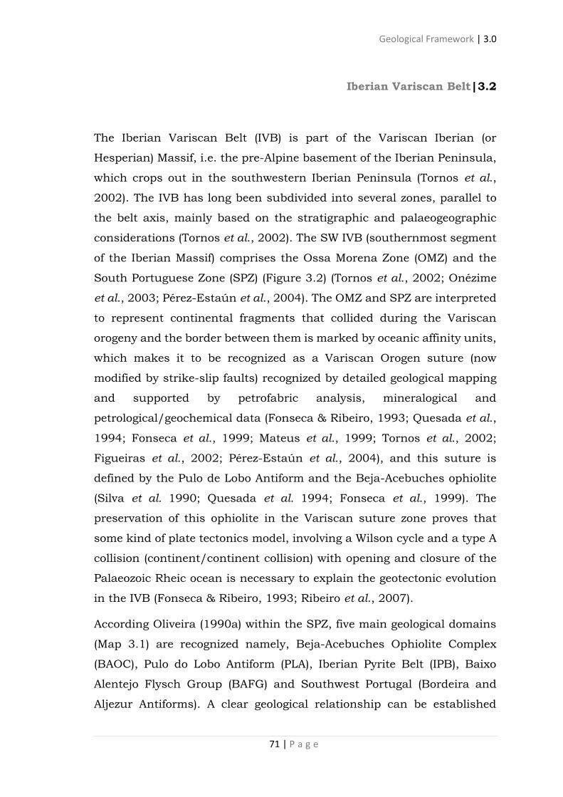
Geological Framework | 3.0
71 | P a g e
Iberian Variscan Belt|3.2
The Iberian Variscan Belt (IVB) is part of the Variscan Iberian (or
Hesperian) Massif, i.e. the pre-Alpine basement of the Iberian Peninsula,
which crops out in the southwestern Iberian Peninsula (Tornos et al.,
2002). The IVB has long been subdivided into several zones, parallel to
the belt axis, mainly based on the stratigraphic and palaeogeographic
considerations (Tornos et al., 2002). The SW IVB (southernmost segment
of the Iberian Massif) comprises the Ossa Morena Zone (OMZ) and the
South Portuguese Zone (SPZ) (Figure 3.2) (Tornos et al., 2002; Onézime
et al., 2003; Pérez-Estaún et al., 2004). The OMZ and SPZ are interpreted
to represent continental fragments that collided during the Variscan
orogeny and the border between them is marked by oceanic affinity units,
which makes it to be recognized as a Variscan Orogen suture (now
modified by strike-slip faults) recognized by detailed geological mapping
and supported by petrofabric analysis, mineralogical and
petrological/geochemical data (Fonseca & Ribeiro, 1993; Quesada et al.,
1994; Fonseca et al., 1999; Mateus et al., 1999; Tornos et al., 2002;
Figueiras et al., 2002; Pérez-Estaún et al., 2004), and this suture is
defined by the Pulo de Lobo Antiform and the Beja-Acebuches ophiolite
(Silva et al. 1990; Quesada et al. 1994; Fonseca et al., 1999). The
preservation of this ophiolite in the Variscan suture zone proves that
some kind of plate tectonics model, involving a Wilson cycle and a type A
collision (continent/continent collision) with opening and closure of the
Palaeozoic Rheic ocean is necessary to explain the geotectonic evolution
in the IVB (Fonseca & Ribeiro, 1993; Ribeiro et al., 2007).
According Oliveira (1990a) within the SPZ, five main geological domains
(Map 3.1) are recognized namely, Beja-Acebuches Ophiolite Complex
(BAOC), Pulo do Lobo Antiform (PLA), Iberian Pyrite Belt (IPB), Baixo
Alentejo Flysch Group (BAFG) and Southwest Portugal (Bordeira and
Aljezur Antiforms). A clear geological relationship can be established

Geological Framework | 3.0
72 | P a g e
between the IPB, the BAFG and the SW Portugal domains (Oliveira,
1990a).
IPB (well-known metallogenic province) can be described as a succession
of three Devonian to Dinantian formations: the Phyllites-Quartzites
Group (PQG), the Volcano-Sedimentary Complex (VSC), and the Culm
(Map 3.1) (e.g., Schermerhorn, 1970).
According to Onézime et al. (2003) the Devonian in the sense of the PQG
corresponds to a passive margin detritic sequence and constitutes the
oldest unit observed to the south of the PLA.
The uppermost unit of the IPB, the Culm, corresponds to a Visean
flyschoid sequence commonly associated with the BAFG (Oliveira, 1983).
However, Onézime et al. (2003) propose to consider the base of the BAFG,
Figure 3.2: Interpretative cross section and map of the SW margin of the Variscan Belt
of Iberia during Variscan times. Modified from Silva et al. (1990) and Quesada (1991).
(a) Plate convergence, subduction and minor oblique collision and partial obduction
during the late Devonian (pre-Fammenian); (b) Generalized oblique collision, lateral
escape of the South Portuguese Zone and formation of second order pull-apart basins
and volcanic alignments in the Iberian Pyrite Belt and Ossa Morena Zone during the
late Devonian-Lower Carboniferous. Not to scale. SPZ, South Portuguese Zone; IPB,
Iberian Pyrite Belt; OMZ, Ossa Morena Zone; BCSZ, Badajoz-Cordoba Shear Zone; PLT,
Pulo de Lobo Terrane (including the Beja-Acebuches Ophiolite). Adapted from Tornos
et al. (2002).

Geological Framework | 3.0
73 | P a g e
the Culm formation, as part of the IPB, both sequences being closely
associated. According to Moreno & González (2004), in the Portuguese
part of IPB, the Culm is called BAFG.
South Portuguese Zone|3.3
The SPZ has been described for many works (e.g. Schermerhorn, 1970;
Oliveira, 1983; Oliveira, 1990b) provides an interpretation synthesis of
the geological environment based on sedimentary processes, volcanism
and synsedimentary tectonism. According to Fonseca & Ribeiro (1993)
and Pérez-Estaún et al. (2004) the SPZ includes Late Devonian - Late
Carboniferous sediments and volcanics deposited in an intra-continental
transtensional setting. The SPZ overstepped the contact with the Iberian
terrane and was deformed in a transpressional regime during the Upper
Carboniferous, with vergence towards the south-west, in a typical thin-
Map 3.1: (a) Geological map of the South Portuguese Zone [after Oliveira, 1990b]; (b)
tectonic map of the South Portuguese Zone. Adapted from Onézime et al. (2003).

Geological Framework | 3.0
74 | P a g e
skinned thrust belt being constituted by Upper Palaeozoic low- to very
low-grade metamorphic rocks (Munhá, 1990; Fonseca & Ribeiro, 1993;
Abad et al., 2001, 2002; Simancas, 2004). The SPZ shows the
characteristic features of a foreland fold-and-thrust belt dominated by
thin-skinned tectonics (Silva et al., 1990; Simancas et al., 2004).
The high-resolution crustal image given by the IBERSEIS seismic
experiment (Figure 3.3) confirms a thrust pattern within the SPZ, which
is characteristic of foreland thrust and fold belts (Simancas et al., 2004).
The thrusts dip to the northeast and merge in the middle crust, indicating
a decoupling zone at this level (Simancas et al., 2004). The figure 3.4
represents the hypothetical framework cross-section of the Aljustrel
structure (SPZ) in the piggy-back system, according to Ribeiro et al.
(2007).
According to Mantero et al. (2011) foreland fold-and-thrust belts are
typical features in the external zones of most orogenic belts. They
generally involve only the sedimentary cover (i.e. thin-skinned style),
although sometimes both the basement and the cover are deformed (i.e.
thickskinned style).
Figure 3.3: a) The IBERSEIS migrated crustal seismic image of SW Iberia; b) hand-
drawing of reflectors in the IBERSEIS profile. Adapted from Simancas et al. (2004).

Geological Framework | 3.0
75 | P a g e
According to Silva et al. (1990), the SPZ was in turn accreted to the OMZ
during the Variscan orogeny, this accretion is also witnessed by the
presence of various mélanges (Onézime et al., 2003). This north directed
subduction of the SPZ under the OMZ parautochthon, widely admitted
nowadays, precludes some of the fore-mentioned models and is in
agreement with the age and distribution of units composing the SPZ
(Onézime et al., 2003).
Structural analysis within the Spanish side of the SPZ supports
continuous south propagating deformation, evolving from early
synmetamorphic thrusting in the internal zone to thin-skinned tectonics
in the southern external domain. Subsequent Visean continental
collision is associated with the deposit of the south propagating flysch
and the present geometry of the SPZ (Onézime et al., 2003).
Also according to the authors, the formations are getting younger toward
the south from the Early/Middle Devonian PLA, the late Devonian-Visean
IBP (Map 3.1). A logical distribution of the main domains from north to
south is also recognized, from the oceanic domain to the north (the BAOC)
and the related PLA accretionary prism, to the foreland basin (i.e., the
south propagating BAFG).
Figure 3.4: Hypothetical cross-section of Mértola, Mira and Brejeira Formations,
emphasizing the piggy-back system. Adapted from Ribeiro et al. (2007).

Geological Framework | 3.0
76 | P a g e
Baixo Alentejo Flysch Group|3.4
The BAFG is mostly a turbidite sequence prograding to SW and with more
than 3 km in thickness (some sectors reach more than 5 km, according
to Fonseca et al., 2015), being an important stratigraphic unit that
covers, in some places by unconformity, more than half of the SPZ
depositional area. The BAFG is composed by three main tectono-
stratigraphic units (from the base to the top): Mértola, Mira and Brejeira
Formations (Oliveira, 1983). These three formations generally trend to dip
towards SW and sometimes, according to the structure, dip to the
opposite side, NE, roughly parallel to the IPB and the OMZ-SPZ
boundary. These formations are dated from Upper Visean, Upper
Serpukhovian-Mid Bashkiriano and Mid Bashkirian-Upper Moscovian,
respectively. Due to the general dip and vergence towards SW units tend
to be younger towards the same direction (Oliveira, 1983).
Mértola Formation|3.5
According to Oliveira (1990b), Mértola Fm. (Figure 3.5) is built up by
sequences of thick- and thin-bedded sandstones, and alternating bands
of shales and thin-bedded siltstones. The sandstone/shale ratio is high.
The sandstones display many of the sedimentary features usually
described for gravity flow sediments (Oliveira, 1990b). Massive and
amalgamated sandstones, fluidized sandstones, slumps, conglomerates,
sand dykes, mud flows and isolated sheeted sandstones are more
common as far as the contact with the Pyrite Belt rocks are approached
(Oliveira, 1990b). This facies distribution demonstrates the close
relationship between the tectonostratigraphic evolution of the IPB and
the flysch sedimentation (Oliveira, 1983). In the Mértola region, this unit
has been divided into five members separated by five shaly horizons,

Geological Framework | 3.0
77 | P a g e
taken as markers beds (Oliveira & Silva, 1988). The members correspond
to sedimentary lobes and the shaly horizons to interlobe sediments. The
sedimentary lobes prograded to SSW. The Mértola Fm. was studied for
palynomorphs in several regions: such as the Neves Corvo mine, Mértola
town, Azenhas section in Guadiana River, Bens Farm, and are given a
late Viséan age (Figure 3.8 [Oliveira et al., 2007; Pereira et al., 2007]).
Mira Formation|3.6
According to Oliveira (1990b), the turbidites of this formation are
commonly thin-bedded and show a sandstone/shale ratio < 1. An
exception is the southeastern area where they have a sandstone/shale
ratio similar to that of the Mértola Fm. (Figure 3.6). The contact with the
Mértola Fm. is marked by a continuous shaly horizon, 50 to 100 m thick,
which yielded goniatites of the GoY zone (Oliveira & Wagner Genthis,
1983; Oliveira, 1990b). The age of this formation is late Viséan to early
Figure 3.5: Mértola Formation outcrop. According to Oliveira (1990b), this unit is built
up by sequences of thick- and thin-bedded sandstones, and alternating bands of
shales and thin-bedded siltstones.
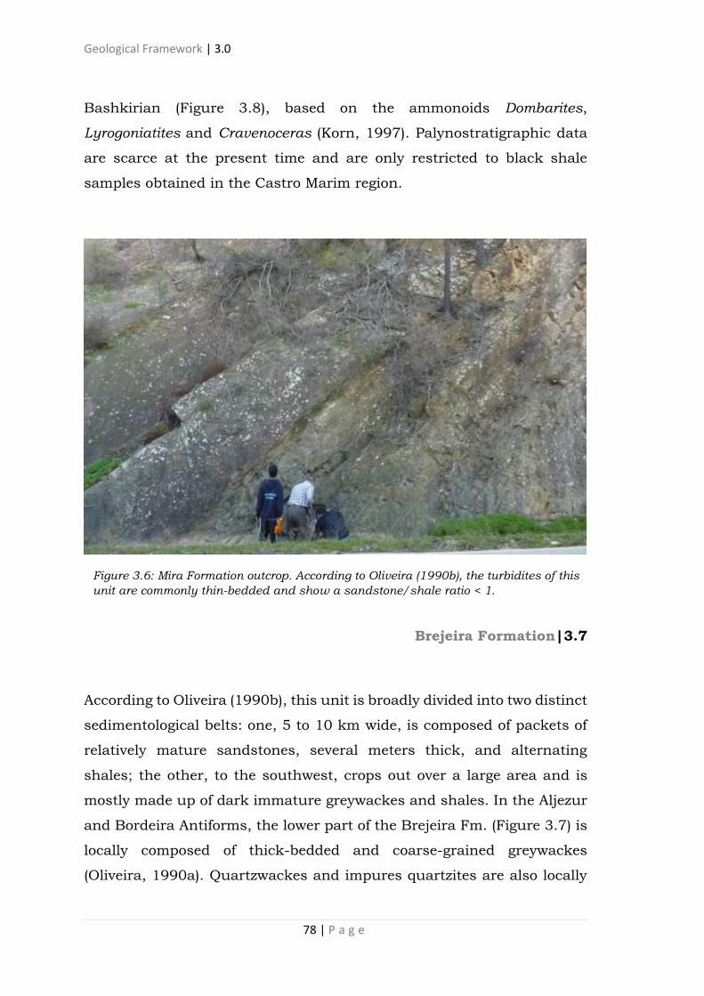
Geological Framework | 3.0
78 | P a g e
Bashkirian (Figure 3.8), based on the ammonoids Dombarites,
Lyrogoniatites and Cravenoceras (Korn, 1997). Palynostratigraphic data
are scarce at the present time and are only restricted to black shale
samples obtained in the Castro Marim region.
Brejeira Formation|3.7
According to Oliveira (1990b), this unit is broadly divided into two distinct
sedimentological belts: one, 5 to 10 km wide, is composed of packets of
relatively mature sandstones, several meters thick, and alternating
shales; the other, to the southwest, crops out over a large area and is
mostly made up of dark immature greywackes and shales. In the Aljezur
and Bordeira Antiforms, the lower part of the Brejeira Fm. (Figure 3.7) is
locally composed of thick-bedded and coarse-grained greywackes
(Oliveira, 1990a). Quartzwackes and impures quartzites are also locally
Figure 3.6: Mira Formation outcrop. According to Oliveira (1990b), the turbidites of this
unit are commonly thin-bedded and show a sandstone/shale ratio < 1.

Geological Framework | 3.0
79 | P a g e
present. In this case, an erosional contact with the underlying rocks of
the Carrapateira Group is discernible. In the Brejeira Fm. turbidites (the
younger unit of the BAFG) palynostratigraphic study revealed 6 miospore
biozones, ranging from the Bashkirian to late Moscovian (Figure 3.8
[Pereira et al., 2007]). These miospore ages are consistent with the local
ammonoid biozonation (Korn, 1997), which mark the local deepening of
the basin floor, probably as a response to the southward moving orogenic
wave (Oliveira et al., 2007).
According to Pereira et al. (2007), the distribution of the palynological
assemblages, supports the southwestward progradation of the turbidites.
The Variscan tectonic deformation in this sector is Kasimovian in age
(Pereira et al., 2007).
According to Oliveira & Wagner Genthis (1983) this formation exhibits
flow directions mainly to the SE and E, with some paleocurrent
measurements indicating flow towards the SW and N.
Figure 3.7: Brejeira Formation outcrop. According to Oliveira (1990b), the southwest of
this unit, crops out over a large area and is mostly made up of dark immature
greywackes and shales.
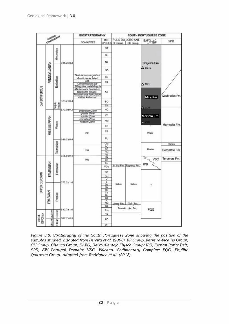
Geological Framework | 3.0
80 | P a g e
Figure 3.8: Stratigraphy of the South Portuguese Zone showing the position of the
samples studied. Adapted from Pereira et al. (2008). FF Group, Ferreira-Ficalho Group;
CH Group, Chanca Group; BAFG, Baixo Alentejo Flysch Group; IPB, Iberian Pyrite Belt;
SPD, SW Portugal Domain; VSC, Volcano- Sedimentary Complex; PQG, Phyllite
Quartzite Group. Adapted from Rodrigues et al. (2015).
Mértola Fm.
Mira Fm.

Geological Framework | 3.0
81 | P a g e
Provenance|3.8
Jorge et al. (2013) suggest that the greywackes from the Mértola and Mira
Fms. show similar modal compositions, while Brejeira greywackes are
more enriched in quartz and have lithoclasts composed mostly by
sedimentary and metasedimentary grains. The source area of Mértola
greywackes is heterogeneous, dominated by rocks with granitoid
composition and minor mafic input (Jorge et al. 2013). The mafic
component becomes residual in greywackes of Mira Fm., where granitoid
source predominates. Greywackes from the Brejeira Fm. exhibit a clear
felsic signature with significant increase in recycled components. All
analyzed shales show geochemical features compatible with provenance
areas of mostly granodioritic composition (Jorge et al. 2013).
Jorge et al. (2013) suggest that Mértola and Mira Fms. underwent
moderate weathering in the source areas, where reduced variation of both
palaeoweathering indices indicates steady-state weathering conditions.
The authors say that the youngest Brejeira Fm. show moderate to intense
weathering as a consequence of a non-steady-state conditions. Shales
from Mértola, Mira and Brejeira Fms., have a more complex history of
chemical weathering associated with multiple cycles of sedimentary
recycling. Pereira et al. (2013) suggest that the sedimentation in the SPZ
from the Visean to the Moscovian is marked by variability in sedimentary
sources, involving the denudation of different crustal blocks and a break
in synorogenic volcanism and Jorge et al. (2013) comment that the
weathering conditions of BAFG sediments source area(s) changed from
moderate to intense probably as a consequence of tectonic instability in
the area (Figure 3.9).
U–Pb detrital zircon spectra from the BAFG show significant differences
between the Mertola–Mira Fms. and the Brejeira Fm. (Rodrigues et al.,
2015). The main peaks in the detrital zircon spectra of the Mértola and

Geological Framework | 3.0
82 | P a g e
Mira Fms. are at 330 Ma, in contrast to the Brejeira Fm., for which the
main peaks are at 615 Ma. Moreover, U–Pb detrital zircon ages of 900–
1100 Ma are encountered in the Brejeira Fm. but are absent in the
Mértola and Mira Fms (Rodrigues et al., 2015).
According to Jorge et al. (2013), petrographic analyses, geochemical
signatures of major and trace elements and multi-element tectonic
discriminant diagrams suggest a continental arc/active margin as the
most prominent origin for BAFG sediments (Figure 3.9). These data also
indicate that an old upper continental crust contributed to the sediments
of the Mira and Brejeira Fm., more pronouncedly to the latter (Figure 3.9).
Still according to the author, collectively, geochemical signatures of three
BAFG formations are compatible with provenance from the SW border of
OMZ mostly, with possible contribution of an external (Avalonian) source
(Figure 3.9). Rodrigues et al. (2015) suggest that the abundance of detrital
zircon in the 500–750 and 900–1100 Ma age range intervals in the
Brejeira Fm. suggests a source region in the Avalon–Meguma terranes
with minor recycling from the SW Portugal Domain (Tercenas Fm.). The
existence of late Ordovician and Silurian zircons in Brejeira turbidites
which have no correspondence in the Gondwana basement of SW Iberia
indicates Laurentia as their most probable source (Figure 3.9 [Pereira et
al., 2013]). The process of formation of Pangea by collision between
Laurentia and Gondwana caused denudation of the two continental
blocks, and the resulting debris were deposited in the SPZ (Figure 3.9
[Pereira et al., 2013]).
The different provenance areas for the units of the BAFG are attributed
to the presence of a physical barrier that was formed during the
development of the foreland basin. This barrier was active from mid-
Visean times and separated the sub-basins where the formations
sediments accumulated (Rodrigues et al., 2015).

Geological Framework | 3.0
83 | P a g e
Figure 3.9: (a) Schematic palaeogeographical reconstruction for Pennsylvanian
times showing the position of the South Portuguese Zone in relation to adjacent
terranes (after Simancas, 2004). (b, c) Geodynamic evolution of the SPZ during the
deposition of the Baixo Alentejo Flysch Group in (b) the Late Serpukhovian and (c)
the Early Bashkirian (adapted from Oliveira et al. 2013). Adapted from Rodrigues
et al. (2015).


85 | P a g e
MATERIALS AND METHODS|4.0
Rock-Eval Pyrolysis|4.1. . . . . . . . . . . . . . . . . . . . . . . . . . . . . . . . . . . .85
Worldview-2 Satellite Images and Airborne Gamma Radiation|4.2. . . . 86
Thorium-Normalization and Hydrocarbon Anomaly|4.3. . . . . . . . . . . . 89
Surface Geochemical Prospecting|4.4. . . . . . . . . . . . . . . . . . . . . . . . . .90
Methods and analysis conditions for headspace-gas chromatography
(HS-GC) and mass-spectrometry by Isotech Laboratories inc. and Isolab
b.v.|4.5. . . . . . . . . . . . . . . . . . . . . . . . . . . . . . . . . . . . . . . . . . . . . . . . 93
Gas Chromatography (GC)|4.6. . . . . . . . . . . . . . . . . . . . . . . . . . . . . . .95
Isotope Ratio Mass Spectrometry|4.7. . . . . . . . . . . . . . . . . . . . . . . . . .98
Static Headspace Gas Chromatography Sampling (Isojar)|4.8. . . . . . .100
Rock-Eval Pyrolysis|4.1
total of 31 samples were collected for rock-eval pyrolysis (22 in
Brejeira Formation, 3 in Mira Formation and 1 in Mértola
Formation [Appendix 10.65]). The laboratorial analyses (using
Rock-Eval 6) were performed by Weatherford Laboratories and Polish
Geological Institute and were financed by Repsol E&P, Partex Oil&Gas
and Polish Geological Institute. All the samples performed by Polish
Geological Institute were selected for rock-eval pyrolysis, however the
Weatherford Laboratories just analyzed samples with TOC higher than
1.0 wt%.
A

Materials and Methods | 4.0
86 | P a g e
Rock is crushed to fine sand particle size (0.125-0.25 mm) and 100 mg
samples are loaded into pyrolysis crucibles (Peters, 1999). The samples
are pyrolyzed under helium at 300°C for 3-4 min, followed by heating at
25°C/min to 550°C. Hydrocarbons (HC; compounds containing only
hydrogen and carbon) and carbon dioxide evolved from organic matter
during heating are measured over time. Each analysis requires about 20
min.
WorldView-2 Satellite Images and Airborne Gamma Radiation|4.2
According to the DigitalGlobe data sheet (DigitalGlobe, 2016), the WV2
was launched in 2009, and is the first high-resolution 8-band
multispectral commercial satellite. The satellite operates at an altitude of
770 km with 46 cm spatial resolution in panchromatic band and 185 cm
for multispectral bands (Table 4.1).
Three images (satellite images courtesy of the DigitalGlobe Foundation),
described in the table 4.1, were used to construct a mosaic (WGS 1984
UTM 29N zone) that covered the all AOI (Figure 4.1 and Table 4.2). From
this mosaic 8 image bands were extracted to be used for the correlation
with gamma radiation (Table 4.1).
The airborne radiometric survey data, used in this work, was operated by
Rio Tinto Zinc Co. (RTZ) in 1991 and was generously donated by the
National Laboratory of Energy and Geology (Geological Survey) from
Portugal. The data were provided with the file format “.grid” and the unit
of measurement is counts per second (cps). In order to convert the cps
values to part per million-ppm (238U and 232Th), percent (40K) and
nanoGray per hour-nGy/h (total count) the standard conversion rate,
suggested by Geosoft (2005), were used (Table 4.3). The distance between
the measurement points was 75 meters and the Mértola and Mira
Formations were entirely covered by the flights. However, the Brejeira Fm.

Materials and Methods | 4.0
87 | P a g e
wasn’t completely covered, and thus the most southern area of the
formation was not analyzed. So, based on kriging method, the thematic
maps were interpolated.
The sample points from airborne gamma survey (with 75m of distance)
were used as references for the pixel value extraction from all the 8
mosaic bands. Therefore, there are 204,972 points with 13 different data:
8 WV2 bands, TC, Th, U and K.
Satellite Band Pixel range nm Resolution (cm)
WorldView-2 1-Coastal 0-255 400 - 450 185
2-Blue 0-255 450 - 510 185
3-Green 0-255 510 - 580 185
4-Yellow 0-255 585 - 625 185
5-Red 0-255 630 -690 185
6-Red edge 0-255 705 - 745 185
7-Near-IR1 0-255 770 - 895 185
8-Near-IR2 0-255 860 - 1040 185
Panchomatic 0-2047 450 - 800 46
Table 4.1: Worldview-2 imagery bands information (DigitalGlobe, 2016).

Materials and Methods | 4.0
88 | P a g e
For each pixel value from bands (from 0 to 255) it was calculated the
average GR value (TC, Th, U and K). The simple xy graphing would not
be sufficient to determine which bands could present the best correlation
for each radiometric variable.
Image DigitalGlobe reference
P002 15JUL26112846
P004 15JUL23113907
P006 14MAR06114313
Units Conversion rate
Total Count cps/nGy/h 23
Thorium cps/ppm 4,5
Uranium cps/ppm 7,5
Potassium cps/% 75
Table 4.2: References of the images used for the
mosaic design.
Figure 4.1: Contours of the images
used for the mosaic design of the
area of interest (AOI).
Table 4.3: Values of standard conversion
rate suggested by Geosoft (2005).

Materials and Methods | 4.0
89 | P a g e
Thus, it was used the Pearson’s correlation coefficient (PC), one of the
most used statistical quantitative method in geosciences, which
measures the degree of (linear) interrelation between two sampled (data
size n) variables, x and y (Mudelsee, 2003). For this thesis, the PC was
calculated using IBM SPSS software.
Thorium-Normalization and Hydrocarbon Anomaly|4.3
As said before, one of most successful models for identifying radiometric
anomalies related to hydrocarbon occurrence was developed by Saunders
et al. (1993). A basic assumption is that whatever changes the
concentration of a radioactive isotope it also changes the concentration
of the other two isotopes, in the case of hydrocarbon presence. According
to the author, if hydrocarbons are not present, 238U, 40K and 232Th should
be present in natural and constant proportions. Lithological and
environmental variables that once were problematic are now suppressed
by the correction of 40K and 238U readings using the TN process (Saunders
et al., 1993).
Based on detailed studies of radiometric measurements in oilfields,
Saunders et al. (1993) developed a relationship between the 238U, 40K and
232Th data in order to help identify the hydrocarbon anomalies (HA). 40K
concentrations appear to be significantly lower over oil and gas fields, and
238U was found to be slightly concentrated in profiles over Alabama Ferry,
Leona, O.S.R., and Lonesome Dove fields, Texas (Saunders et al., 1993;
Prost, 2014). 232Th is considered to be highly “retained” in rocks and local
soils, not being affected by the hydrocarbon ascension. Based on these
assumptions, Saunders et al. (1993) defined the “ideal” 40K and 238U as:
Ki = (Kav/Thav) X Ths (Equation 1)
Ui = (Uav/Thav) X Ths (Equation 2)

Materials and Methods | 4.0
90 | P a g e
where the subscript “s” refers to the measured or sampled value, “i” is
the ideal value and “av” is the mean value of the studied area, generally
at least 5 times greater than the predicted anomaly. This can result if the
area to be investigated is of several km2. The difference between the
measured values and the ideal values is then calculated (Saunders et al.,
1993):
KD = (Ks-Ki)/Ks (Equation 3)
UD = (Us-Ui)/Us (Equation 4)
In hydrocarbon presence, KD should decrease and UD generally
increases. To capitalise upon these 2 relationships, the same authors
defined a new parameter, known as DRAD:
DRAD = UD – KD (Equation 5)
Therefore, HA is normally characterised by positive values of DRAD and
negative values of KD and UD (sometimes positive values) (Saunders et
al., 1993).
Surface Geochemical Prospecting|4.4
The presence of near-surface migrated hydrocarbons can provide strong
evidence an active petroleum system is present as well as critical
information on source, maturity and migration pathways (Abrams et al.,
2001; Abrams, 2013). When applied to hydrocarbon exploration, soils,
sediments, air, water and rock samples can be sampled and tested
through various analytical methods (Bandeira de Mello et al., 2007).
The procedures for surface geochemical sampling campaign begin with
preliminary planning actions, such as area selection (target), geological
base maps, satellite imagery, etc., as well as choose the most suitable
months for field operations (Bandeira de Mello et al., 2007). Once the
research area has been established, the efforts are focused on potential

Materials and Methods | 4.0
91 | P a g e
hydrocarbon systems (conventional or unconventional), thus defining the
positioning of the sampling points. After these adjustments, the most
appropriate sampling methodologies and respective standard procedures
are defined (Figure 4.2 [Bandeira de Mello et al., 2007]).
According to Abrams (2013) the light hydrocarbons require special
handling and containers to limit volatile loss and prevent post sampling
microbial alteration. Several methods are used for direct hydrocarbon
sampling such as probe and headspace for free gases, blender and
disrupter for occluded gases, acid extraction for adsorved gases and
sorbing fibers (Bandeira de Mello et al., 2007).
In general, the research methodologies in surface geochemistry aims to
quantify hydrocarbons movement in a medium, on a time scale (Tedesco,
1995). Under standard conditions for temperature and pressure (25ºC
and 1 atm) light hydrocarbons (methane [CH4], ethane [C2H6], propane
[C3H8], isobutane [i-C4H10] and n-butane [n-C4H10]) are present, on the
surface, in the gas format. Hydrocarbons of slightly larger molecular
Planning Sampling Lab
Statistics
Maps Graphs Tables Reports
Analytical results
Integration and interpretation
Wells
Field records
Geochemical data base
GIS (Geographic information system)
Satellite image
Topography
Geology
Geophisics
Figure 4.2: General scheme of the activities relates to surface geochemical prospection
of hydrocarbons. Adapted from Bandeira de Mello et al. (2007).

Materials and Methods | 4.0
92 | P a g e
weights such as n-pentane (nC5) and n-hexane (nC6) are present, on the
surface, in the liquid format. However, they can be found as gas (vapor)
just with a small increase of the temperature. In the soil, light
hydrocarbon can “stay” in three formats: (1) as a free gas in the effective
porosity; (2) as interstitial hydrocarbon, or occlusion in the pore space
between the grains; (3) adsorved in the sediment particles or in the
carbonate cement (Schumacher & Abrams 1996).
The sampled volume goes on to review research investigations and case
history studies of every gas that might act as an indicator or pathfinder
and to elaborate the models developed to explain the resulting
observations (Hale, 2000). Gas composition by itself will not provide
sufficient information to fully evaluate anomalous sediment gas origin.
Compound specific isotopic analysis from IR GC-MS analysis is critical
to determine gas maturity and source facies as well as potential mixing
with in-situ derived gases and secondary alterations (Abrams, 2005;
Abrams & Dahdah, 2011; Abrams, 2013). Only where these are overcome
effectively can the detection of trace quantify of gases derived from
mineral deposits and petroleum accumulations at depth (Hale, 2000).
The collection of all samples was performed using Isojars (Figure 4.3B),
with distilled water and a bactericide added to inhibit any bacterial
activities. Twenty-seven soil samples were collected for this study, using
a drilling machine (F and P samples [Figure 4.3D and Appendix 10.64]),
a metal tube and a hammer (SPZ samples [Figure 4.3A, C and Appendix
10.64]). Thirty-one water samples (W samples) were collected from
artesian wells, boreholes and springs (Appendix 10.64).

Materials and Methods | 4.0
93 | P a g e
Methods and analysis conditions for headspace-gas
chromatography (HS-GC) and mass-spectrometry by Isotech
Laboratories Inc. and Isolab b.v.|4.5
In order to achieve the best performance when using HS-GC, careful
attention should be used in sample preparation and instrument setup.
Key issues to address when setting up HS-GC systems include
minimizing system dead volume, maintaining inert sample flow paths,
and achieving efficient sample transfer (Restek, 2000).
According to Isotech (2014), the procedure for taking cuttings samples in
IsoJars are:
1. Put the sample in jar (approximately 1 cup);
2. Only add water to reach the line on the label;
3. Do not fill the jar with water as the headspace gap is needed to allow
gas to desorb into the gap;
4. Leave about a 1-inch gap between the water and top of the jar;
5. Add 10 drops of the dilute bactericide, Benzalkonium Chloride, to the
jar;
6. Screw the lid on as tight as possible;
Figure 4.3: A) Hammer; B) Isojar, by
Isotech (Weatherford); C) Tubes used for
soil sampling; D) Drilling machine used
for deeper sampling.

Materials and Methods | 4.0
94 | P a g e
7. Tape the lid to keep it tight and from vibrating loose during shipment.
Tape in same direction (clockwise) that the lid is screwed on.
According to Abrams (2013), the bactericide is used to prevent in-situ
microbial activity. The amount of bactericide required to prevent
microbial activity has not been rigorously examined. To the best of the
author’s knowledge, no comprehensive studies have been conducted to
evaluate the effectiveness of these anti-bacterial agents, how much is
required, or if the anti-bacterial agents impact the geochemistry results.
Molofsky et al. (2016) suggests that an open-system collection technique
is prone to loss of exsolving gases as methane, resulting in low-biased
concentrations associated with the water samples. According to Parker &
Britt (2012), the VOC most susceptible to loss is
dichlorodifluoromethane, with 76% loss (Henry’s constant 3.0 atm
m3/mol). Methane is significantly more volatile than the VOCs evaluated
by Parker & Britt (2012), according to Molofsky et al. (2016).
Composition analysis of mudgas samples (including CO2 concentration)
(by Isolab b.v.):
For composition analysis of samples with low gas concentration like
mudgas samples in isotubes or isojars, an Agilent 7890B GC (Agilent
Technologies, Santa Clara, US) equipped with a 30m 0.32mm Gaspro
column and a 50m 0.32mm Porabond Q column (both from Agilent) is
used. The Gaspro column is coupled to a flame ionization detector and
used for analysis of hydrocarbons. The Porabond Q column is coupled to
a TCD detector and used for the analysis of the CO2 concentration.
Samples are injected into a heated injection valve on the GC using a
gastight syringe. The detector responses are calibrated against a
reference gas (Scott Specialty Gases Netherlands BV, Breda, The
Netherlands) several times a day.
Minimum concentrations: ca. 1 ppm for methane to 0.1 ppm for pentane
and ca. 50 ppm for CO2.

Materials and Methods | 4.0
95 | P a g e
Analysis of carbon isotopes of methane (by Isolab b.v.)
Carbon isotopes of methane are analyzed with an Agilent 6890N GC
(Agilent Technologies, Santa Clara, US) interfaced to a Finigan Delta S
IRMS (Finigan is now part of Thermo Scientific, Bremen, Germany) using
a Finigan GC-C II interface. The GC is equipped with a 12m, 0.32mm
molsieve column (Agilent) and an injection valve. Samples are calibrated
regularly against a calibration standard and results are reported in
promille vs. vPDB.
Minimum concentration: ca. 25-50 ppm.
Gas Chromatography (GC)|4.6
All collected samples were analyzed by GC (58 water and soil samples),
for molar composition purpose (CO2, C1, C2, C3, nC4, iC4, nC5 and iC5),
being 40 from Brejeira Fm. and 18 from Mira Fm.
Gas chromatography is a chromatographic analytical technique for
separating the volatile compounds of various mixtures. Basically,
according to Sparkman et al. (2011), the operating principle of GC
involves volatilization of the sample in a heated inlet or injector of a gas
chromatograph, followed by separation of the components of the mixture
in a specially prepared column (Figure 4.4).
The liquid or gas mixture is injected into a capillary silica column (typical
dimensions: 30 m long, 0.32 mm ID). This Column is coated by a
stationary phase which consist of a liquid or solid film from about 0.25
up to 30 μm thick (Figure 4.4). The temperature of injector and detector
can be adapted according nature of the analyzed sample and is usually
set to about 25 degrees above the boiling point of the highest boiling
component of interest. To transport the analytes (i.e. “the sample being
analyzed", according to McGraw-Hill, 2003, p.23) through the column, a

Materials and Methods | 4.0
96 | P a g e
mobile phase, usually consisting of helium or hydrogen is used. This
mobile phase has a typical flow of about 1-4 ml/min depending on the
application and column dimensions (Figure 4.4).
Temperature control can be either isothermal or programmed to increase
with analysis time continuously or in stages. Proper choice of column and
operating conditions (flow rate and temperature) results in separations to
enable interference-free measurement of the desired components of the
mixture (Peters et al., 2005; Rechsteiner Jr. et al., 2015).
As the analysis cycle progresses the separated components elute from the
column and emerge at the end of the column at different times and can
be detected (progress into the detector.). The time (retention time) that
has passed between sample introduction and the emergence of the
individual analyte bands-the peaks-is, under given conditions,
characteristic of the individual analytes, while the size—height or area—
of the individual peaks is proportional to their amount (Kolb & Ettre,
2006; Rechsteiner Jr. et al., 2015). The retention time of the component
is qualitative, while the area under the curve is quantitative. Calibration
samples are used to relate known component area to the concentration
of the same component in unknown samples (Rechsteiner Jr. et al.,
2015).

Materials and Methods | 4.0
97 | P a g e
According to Grob (2004), the separation depends on the ability of each
component in the mixture to become a sorbate (i.e. “substance that has
been either adsorved or absorbed", according to McGraw-Hill, 2003,
p.352 [Figure 4.5]). Once the column packing has been saturated (i.e.,
when it is no longer able to sorb more components), the mixture then
flows through with its original composition (Figure 4.6 [Grob, 2004]).
Figure 4.4: Detailed view of a typical gas chromatograph used to separate
mixtures of compounds. The blow-up (bottom) shows the separation of
compounds during movement down the chromatographic column, which
results from their repeated partitioning between the mobile and stationary
phases. Adapted from Peters et al. (2005).
Figure 4.5: Difference between absorption and
adsorption. Adapted from Miller (2005).
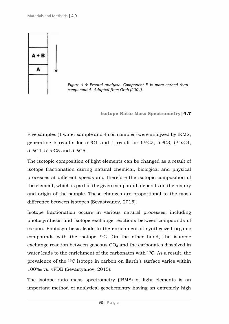
Materials and Methods | 4.0
98 | P a g e
Isotope Ratio Mass Spectrometry|4.7
Five samples (1 water sample and 4 soil samples) were analyzed by IRMS,
generating 5 results for δ13C1 and 1 result for δ13C2, δ13C3, δ13nC4,
δ13iC4, δ13nC5 and δ13iC5.
The isotopic composition of light elements can be changed as a result of
isotope fractionation during natural chemical, biological and physical
processes at different speeds and therefore the isotopic composition of
the element, which is part of the given compound, depends on the history
and origin of the sample. These changes are proportional to the mass
difference between isotopes (Sevastyanov, 2015).
Isotope fractionation occurs in various natural processes, including
photosynthesis and isotope exchange reactions between compounds of
carbon. Photosynthesis leads to the enrichment of synthesized organic
compounds with the isotope 12C. On the other hand, the isotopic
exchange reaction between gaseous CO2 and the carbonates dissolved in
water leads to the enrichment of the carbonates with 13C. As a result, the
prevalence of the 13C isotope in carbon on Earth’s surface varies within
100‰ vs. vPDB (Sevastyanov, 2015).
The isotope ratio mass spectrometry (IRMS) of light elements is an
important method of analytical geochemistry having an extremely high
Figure 4.6: Frontal analysis. Component B is more sorbed than
component A. Adapted from Grob (2004).

Materials and Methods | 4.0
99 | P a g e
sensitivity and accuracy of measurement of isotope ratios. It can be
divided into three fundamental parts, namely the ionization source, the
analyser, and the detector (Figure 4.7). The main function of the mass
analyser is to separate, or resolve, the ions formed in the ionization
source by their mass to charge ratios (m/z) furnishes the molecular
weight and chemical formula of compounds and their relative amounts
and offers nondestructive examination of the sample (Ashcroft, 1997;
Speight, 2001; Sevastyanov, 2015).
Since the relative isotopic composition can be measured with greater
accuracy than the absolute isotopic composition, to represent the relative
isotopic composition of light elements the quantity δ (delta), which is
calculated by the following formula (Sevastyanov, 2015):
δ = (Rx-Rstd)/Rstd) x 1000 (Equation 6)
where “R” is the ratio of the abundance of the heavy isotope to the light
isotope, “x” is an index, indicating the measured sample, “std” is an index
denoting the standard sample. The value of R for the stable isotopes of
hydrogen can be written as D/H, for the carbon isotopes 13C/12C, for the
nitrogen isotopes 15N/14N, for the oxygen isotopes 18O/16O, etc. The value
of δ is expressed in thousandths (per mil), which are indicated by ‰. A
Figure 4.7: Schematic overview of the GC-IRMS solution. The isotope ratio mass
spectrometry can be divided into three fundamental parts, namely the ionization
source (A), the analyser (B), and the detector (C). Adapted from Thermo SCIENTIFIC
(2014).

Materials and Methods | 4.0
100 | P a g e
positive value of δ means that the ratio of the heavy isotope to the light
one in the analyzed sample is greater than in the standard sample
(Sevastyanov, 2015).
The value of δ is calculated by measuring the intensity of ion signals in
the isotope mass spectrometer and recorded, for example for carbon, as
δ13C vs. vPDB. Usually, for pure gases the reproducibility of the results
of isotopic analysis is ±0.1‰ or better (Sevastyanov, 2015).
The resolution ® of a mass analyzer, or its ability to separate two peaks,
is defined as the ratio of the mass of a peak (M1) to the difference in mass
between this peak and the adjacent peak of higher mass (M2) (Ashcroft,
1997).
R = M1/(M2-M1) (Equation 7)
According to Bandeira de Mello et al (2007) for the determination of light
hydrocarbon origin, thermogenic or biogenic, the sample with higher gas
concentration, often methane, is used for stable carbon isotope analysis
(δ13C).
Static Headspace Gas Chromatography Sampling (Isojar)|4.8
Some samples need to be modified for the specific requirement of a
particular analytical technique (Kolb & Ettre, 2006). Most consumer
products and geological samples (as hydrocarbons) are composed of a
wide variety of compounds that differ in molecular weight, polarity, and
volatility (Restek, 2000).
Most of these cleanup techniques use some type of initial extraction
procedure such as solvent extraction, solid-phase extraction, or
supercritical-fluid extraction. A number of solvent-less procedures to
collect the analytes from the samples were developed for the analysis of
volatile organic compounds (Moldoveanu & David, 2002). However, if the

Materials and Methods | 4.0
101 | P a g e
interesting is in highly volatile compounds, it can use an inert gas for this
purpose; gas is an ideal ‘‘solvent’’ for volatile compounds, since it is easy
to handle and is available in a much higher purity than most organic
solvents. This is an aspect that is particularly important for traces
analysis. A gas extract is ideally suited for analysis by GC, and this
combination is called ‘‘headspace–gas chromatography’’ (HS-GC
sampling), the fastest and cleanest method for analyzing volatile organic
compounds. A headspace sample is normally prepared in a vial
containing the sample, the dilution solvent, a matrix modifier like a
bactericide, and the headspace (Restek, 2000; Kolb & Ettre, 2006).
Volatile components from complex sample mixtures can be extracted
from non-volatile sample components and isolated in the headspace or
vapor portion of a sample vial. An aliquot of the vapor in the headspace
is delivered to a GC system for separation of all of the volatile components
(Restek, 2000).
These gas sampling techniques can be classified into two general groups,
“static headspace” and “dynamic headspace” (Figure 4.8). Static
headspace techniques are those that collect the analytes (and possibly
part of the matrix) from a closed vessel where the sample is assumed to
be in equilibrium with its vapors at a specific temperature and pressure,
in a single step or by stepwise repeating of the extraction (multiple
headspace extraction) (Figure 4.8 [Moldoveanu & David, 2002; Kolb &
Ettre, 2006]).
Dynamic headspace techniques remove analytes (and possibly part of the
matrix) from the sample in a stream of gas flowing over or through the
sample and processes them further for analysis, also by stripping the
volatiles (dynamic headspace) by a continuous flow of an inert purge gas
(Figure 4.8 [Moldoveanu & David, 2002; Kolb & Ettre, 2006]). Headspace
type separations of the analytes from the sample significantly simplify the
matrix and are common cleanup procedures selected for the analysis of
volatile compounds (Moldoveanu & David, 2002; Kolb & Ettre, 2006).
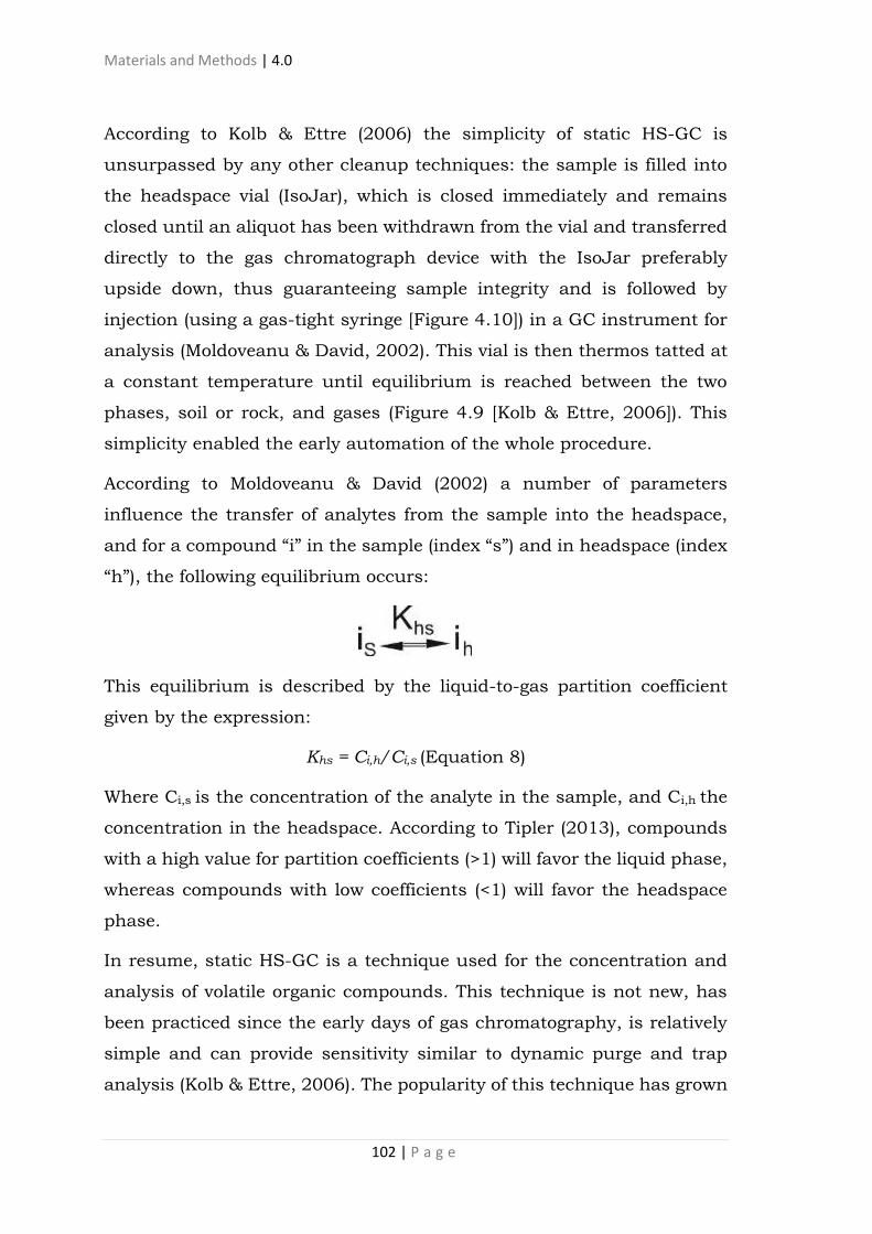
Materials and Methods | 4.0
102 | P a g e
According to Kolb & Ettre (2006) the simplicity of static HS-GC is
unsurpassed by any other cleanup techniques: the sample is filled into
the headspace vial (IsoJar), which is closed immediately and remains
closed until an aliquot has been withdrawn from the vial and transferred
directly to the gas chromatograph device with the IsoJar preferably
upside down, thus guaranteeing sample integrity and is followed by
injection (using a gas-tight syringe [Figure 4.10]) in a GC instrument for
analysis (Moldoveanu & David, 2002). This vial is then thermos tatted at
a constant temperature until equilibrium is reached between the two
phases, soil or rock, and gases (Figure 4.9 [Kolb & Ettre, 2006]). This
simplicity enabled the early automation of the whole procedure.
According to Moldoveanu & David (2002) a number of parameters
influence the transfer of analytes from the sample into the headspace,
and for a compound “i” in the sample (index “s”) and in headspace (index
“h”), the following equilibrium occurs:
This equilibrium is described by the liquid-to-gas partition coefficient
given by the expression:
Khs = Ci,h/Ci,s (Equation 8)
Where Ci,s is the concentration of the analyte in the sample, and Ci,h the
concentration in the headspace. According to Tipler (2013), compounds
with a high value for partition coefficients (>1) will favor the liquid phase,
whereas compounds with low coefficients (<1) will favor the headspace
phase.
In resume, static HS-GC is a technique used for the concentration and
analysis of volatile organic compounds. This technique is not new, has
been practiced since the early days of gas chromatography, is relatively
simple and can provide sensitivity similar to dynamic purge and trap
analysis (Kolb & Ettre, 2006). The popularity of this technique has grown
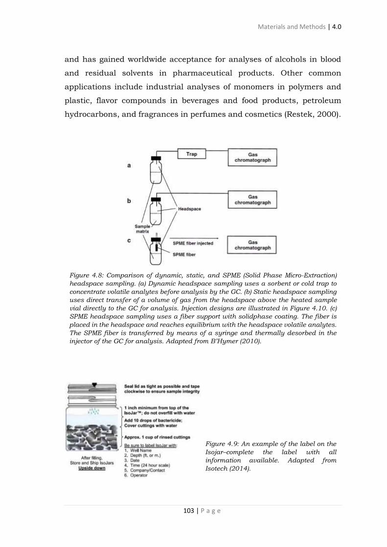
Materials and Methods | 4.0
103 | P a g e
and has gained worldwide acceptance for analyses of alcohols in blood
and residual solvents in pharmaceutical products. Other common
applications include industrial analyses of monomers in polymers and
plastic, flavor compounds in beverages and food products, petroleum
hydrocarbons, and fragrances in perfumes and cosmetics (Restek, 2000).
Figure 4.8: Comparison of dynamic, static, and SPME (Solid Phase Micro-Extraction)
headspace sampling. (a) Dynamic headspace sampling uses a sorbent or cold trap to
concentrate volatile analytes before analysis by the GC. (b) Static headspace sampling
uses direct transfer of a volume of gas from the headspace above the heated sample
vial directly to the GC for analysis. Injection designs are illustrated in Figure 4.10. (c)
SPME headspace sampling uses a fiber support with solidphase coating. The fiber is
placed in the headspace and reaches equilibrium with the headspace volatile analytes.
The SPME fiber is transferred by means of a syringe and thermally desorbed in the
injector of the GC for analysis. Adapted from B’Hymer (2010).
Figure 4.9: An example of the label on the
Isojar–complete the label with all
information available. Adapted from
Isotech (2014).

Materials and Methods | 4.0
104 | P a g e
Figure 4.10: The designs of static headspace injection systems used for the analyzes.
The gas-tight syringe system uses a syringe to collect and transfer a headspace aliquot
to the GC. Adapted from B’Hymer (2010).

105 | P a g e
THEORY OF HYDROCARBON SEEPS|5.0
Total Petroleum System and Petroleum Seepage System|5.1. . . . . . . .105
Seeps Classification|5.2. . . . . . . . . . . . . . . . . . . . . . . . . . . . . . . . . . . 106
Migration Mechanism|5.3. . . . . . . . . . . . . . . . . . . . . . . . . . . . . . . . . .109
Geochemistry of Gases|5.4. . . . . . . . . . . . . . . . . . . . . . . . . . . . . . . . .111
Why is important to know the seeps?|5.5. . . . . . . . . . . . . . . . . . . . . .112
Worldwide Seeps|5.6. . . . . . . . . . . . . . . . . . . . . . . . . . . . . . . . . . . . . .114
Total Petroleum System and Petroleum Seepage System|5.1
n important concept, for hydrocarbon seeps research, is the
“Petroleum Seepage System” (PSS), defined by Abrams (2005) as
“the interrelationships among total sediment fill, tectonics
(migration pathway), hydrocarbon generation (source and maturation),
regional fluid flow (pressure regime and hydrodynamics), and near
surface processes (zone of maximum disturbance)”. The PSS is part of the
Total Petroleum System (TPS), that according to Magoon & Schmoker
(2000) describe the entire hydrocarbon-fluid system in the lithosphere
(that can be mapped), including the essential elements and processes
required for oil and gas accumulations, migrations, and seeps. The
concept presumes that migration pathways must exist, either now or in
the past, connecting the provenance with accumulations (Etiope, 2015).
Seeps are not an exception, but a common, integral component of a TPS.
The PSS would then be the connection between the TPS and Earth’s
A

Theory of Hydrocarbon Seeps | 5.0
106 | P a g e
surface. Abrams (2005) also indicated that “Understanding the PSS,
hence petroleum dynamics of a basin, is key to understanding and using
nearsurface geochemical methods for basin assessment and prospect
evaluation.” TPS and PSS concepts call attention to the fact that
petroleum accumulations are not totally closed, isolated, and sealed
compartments accumulations (Etiope, 2015). Gas (and oil) frequently
leak from reservoirs through cap rocks, even in large and productive
fields, implying that perfect sealing is not necessary for having a
commercial reservoir. Seeps are not a problem, but an opportunity
(Etiope, 2015).
Seeps Classification|5.2
Natural gas seepage is the steady or episodic, slow or rapid, visible or
invisible flow of gaseous hydrocarbons from subsurface sources to
Earth’s surface (Etiope, 2015).
The rate and volume of hydrocarbon seepage to near-surface sediments
controls the surface geological, geophysical, biological, and geochemical
expression (Figure 5.1 [Roberts et al., 1990]) which can range from
macroseepage to microseepage (Abrams, 2013). The surface expressions
of natural gas seepage can be classified on the basis of spatial dimension,
visibility, and fluid typology, as summarized in the following scheme
(Etiope, 2015):

Theory of Hydrocarbon Seeps | 5.0
107 | P a g e
Macroseeps (or seeps) are “channelled” flows of gas, typically related to
fault systems. Gas flux is expressed in terms of mass/time (e.g., kg/day
or tons/year). This surface macroseeps (visible gas vents or oil leaks from
the soil or rock outcrops) are generally an indication of a fault in an active
PSS (Abrams, 2005) belonging to a TPS (Magoon & Schmoker, 2000;
Etiope, 2009a).
Microseepage is the slow, continual loss or episodic loss of methane and
light alkanes from gas-oil-prone sedimentary basins where thermal
degradation of indigenous organic matter is occurring (Figure 5.2 [Etiope
& Klusman, 2002; Etiope, 2009c; Etiope, 2015]). Is basically the
pervasive, diffuse exhalation of gas from soil, independent of the presence
of macroseeps (Etiope, 2015).
Microseepage is assumed to be a general phenomenon driven by
buoyancy of the gas phase relative to connate water (Klusman & Saeed,
1996; Matthews, 1996; Etiope, 2015). The migration is vertical, with
frequent lateral displacement by faulting and flow through carrier beds
toward basin margins (Figure 5.3 [Thrasher et al., 1996; Rostron & Toth,
1996]). Field measurements have indicated that microseepage is
Figure 5.1: Possible model of hydrocarbon microseepage-related alteration over
petroleum deposits. Adapted from Saunders et al. (1999).

Theory of Hydrocarbon Seeps | 5.0
108 | P a g e
enhanced along faults and fractures that also serve as significant
migration pathway (channels) for increased rate of flow by microbubbles,
especially those produced by neotectonics, and can have strong seasonal
variations (Figure 5.3 [Varhegyi et al., 1992; Etiope & Lombardi, 1996;
Etiope, 1998; Kostakis & Harrison, 1999; Brown, 2000, Klusman, 2003;
Etiope & Klusman 2010, Etiope, 2015]).
Sometimes the term “microseeps” is used in the scientific literature,
especially in the marine environment (e.g., Hovland et al., 2012) to define
relatively smaller seeps, not observable, for example, by hydroacoustic
methods. However, the term can be misleading as it may be confused
with microseepage. The classification in the above scheme is, in theory,
valid for either subaerial (landbased) or underwater (marine and lake)
environments (Etiope, 2015).
According to Etiope (2004), potentially areas of microseeps comprise all
sedimentary basins with hydrocarbon generation processes at depth: this
area is estimated to be around 43,366,000 km2 leading to a global
emission of CH4.
Figure 5.2: Sketch of geological methane production and release. Adapted from Etiope
& Klusman (2002).

Theory of Hydrocarbon Seeps | 5.0
109 | P a g e
Migration Mechanism|5.3
Gas seepage implies the long-distance movement of gas that can be on
the order of several kilometers. However, according to Hale (2000) the
relatively slow gas diffusion rates in rocks of low porosity at depth have
brought the contribution of diffusion to long-distance gas migration into
question. The half-life of Rn is so short that its persistence and detection
after transport by diffusion over tens or hundreds of meters is extremely
unlikely (Hale, 2000).
The release of hydrocarbon gases from reservoirs creates the potential for
it to move into near-surface environments through natural and human-
made pathways (Figures 5.2 and 5.3 [Stolp et al., 2006]). Natural
pathways include fractures through the rock layers and voids between
the grains of rock. Human-made pathways can be created when different
types of wells are drilled (Stolp et al., 2006). Regional structural and
stratigraphic features influence the storage of gases, being lighter than
air tends to vertical migration from subsurface accumulations of
hydrocarbons, whether or not they are commercially significant (Figures
5.2 and 5.3 [Eltschlager et al., 2001; Etiope, 2015]). Seepage along faults
can be more an effusive process, rather than microseepage (Etiope &
Klusman, 2002). However, pressure gradients cause gases to migrate to
areas of lower pressure. These migrations may be in directions other than
vertical. Natural overburden pressure is a mechanism that force gas to
the surface (Eltschlager et al., 2001).
The existence of this vertical or near-vertical migration has been
controversial for many years. Arguments against it have included the
following. (1) If reservoirs leaked enough to be detected, they would have
long ago been depleted. (2) If seepage did occur, it would be deflected by
groundwater movements, and anomalies would be displaced laterally for
relatively long distances (Saunders et al., 1999). The ways in which gases

Theory of Hydrocarbon Seeps | 5.0
110 | P a g e
experience dispersion in the subsurface natural environment are more
diverse and less well characterized than mechanisms of dispersion in the
solid and liquid phases. (Hale, 2000). Two main categories of fluid
migration mechanisms exist: (1) diffusion, ruled by Fick’s Law, where gas
moves by concentration gradients; and (2) advection, ruled by Darcy’s
Law, where movement is determined by pressure gradients (Etiope,
2015). Advection is the leading mechanism for seeps and microseepage
(Etiope, 2015). However, Hale (2000) argues that for migration in the gas
phase, diffusion and mass flow are both well-established mechanisms
and each has a role to play in gas transport in the crust. Their relative
contributions to gas migration at different positions in the crust is less
certain. A more controversial mechanism, applicable to gas transport
through groundwater, is gas streaming (Hale, 2000).
Buoyant hydrocarbon microbubbles rising through the water-filled
network of fractures, joints, and bedding planes provide a logical
mechanism for vertical migration of light hydrocarbons from reservoirs to
the surface and commonly occupy the pore voids in rocks, overburden
and soil (Figure 5.3 [Saunders et al., 1999; Hale, 2000]). Kristiansson &
Malmqvist (1982) and Malmqvist & Kristiansson (1984, 1985)
hypothesize that, in the zone of saturation, pressure gradients and
pressure shocks cause over-saturation, leading to the formation of gas
bubbles. These streams upward at a comparatively rapid rate until they
reach the water table (any gas that dissolves in groundwater could, given
the appropriate conditions, migrate by streaming) and mix with the soil
air. The resulting mixture is then driven slowly further upward by the
pressure gradient caused by the bubble stream (Hale, 2000).

Theory of Hydrocarbon Seeps | 5.0
111 | P a g e
Geochemistry of Gases|5.4
Attempts to detect light hydrocarbon microseeps in the 1930s mark the
origins of gas geochemistry (Hale, 2000). In the past, microseepage was
investigated for hydrocarbon exploration with alternate outcomes and
opinions (Philp & Crisp 1982; Tedesco, 1995). Progressive sophistication
has yielded techniques to characterize effectively microseeps both
onshore and offshore. Regional surveys involving the determination of
light hydrocarbons adsorved into soil have contributed to successful
petroleum prospecting (Hale, 2000).
A compilation of papers edited by Aminzadeh et al. (2013) focused on the
use of new technologies designed to image seeps for exploration and field
development applications. Such invisible seepage can easily be detected
using soil-gas analyses, revealing anomalous concentrations of gaseous
hydrocarbons in the soil (Figure 5.3), and using a closed-chamber
technique that allows determinations of gas flux to the atmosphere
(Etiope, 2015).
In particular, the assessment of the origin of seeping gas is a key task for
understanding, without drilling, the subsurface hydrocarbon potential,
genesis and quality, e.g. the presence of shallow microbial gas, deeper
thermogenic accumulations, the presence of oil and non-hydrocarbon
undesirable gases (CO2, N2, H2S). Low quality, biodegraded petroleum can
also be recognized, before drilling, through specific geochemical features
of the seeping gas (Etiope, 2004). The geochemical analysis of seeping
gas, in particular, can be effective to understand the potential and nature
of subsurface accumulations (Etiope, 2009a, 2009b).

Theory of Hydrocarbon Seeps | 5.0
112 | P a g e
Why is important to know the seeps?|5.5
Saunders et al. (1999) reports that since 1976 have used various
combinations of surface hydrocarbon microseepage and related
alteration methods of petroleum exploration, resulting in the discovery of
38 oil and gas fields, mostly in regions where seismic has had limited
effectiveness.
Many large oil and gas fields in North America, Europe, the Caspian
Basin, Asia, and the Caribbean were, in fact, discovered after drilling in
the vicinity of seeps (Link, 1952; Macgregor, 1993; Abrams, 2005). More
generally, gas and oil seeps are important for four main reasons (Etiope,
2009a, 2009b):
- Seeps can be indicators of petroleum or natural gas reservoirs;
- Seeps indicate the occurrence of a fault (according to Etiope [2015], gas
in fact, follows preferential pathways of movement [less resistance paths],
as determined by fractures and faults);
Figure 5.3: Possible microseepage paths up through the network of fractures,
joints, and bedding planes. Adapted from Saunders et al. (1999).

Theory of Hydrocarbon Seeps | 5.0
113 | P a g e
- Seeps can represent a geo-hazard for societal community and industry;
- Seeps are natural sources of greenhouse gas.
According to Schumacher (2012), the surface manifestations of
hydrocarbon microseepage can take many forms, including:
- anomalous hydrocarbon concentrations in soils, sediments, waters, and
atmosphere (Figures 5.3 and 5.1);
- microbiological anomalies;
- mineralogic changes such as formation of calcite, pyrite, uranium,
elemental sulfur, and magnetic iron oxides and sulfides (Figure 5.1);
- bleaching of redbeds;
- clay-mineral changes (Figure 5.1);
- acoustic anomalies;
- radiation anomalies;
- electrochemical changes;
- biogeochemical changes and geobotanical anomalies.
According to Hale (2000), if a mineral deposits or petroleum
accumulations are judged or can be shown to liberate a gas into a porous
medium such as overlying rock, overburden or soil then, in the simplest
case, the gas will form a broad spherical halo.
Chemical alterations of near-surface sediments by carbon dioxide and
hydrogen sulfide, produced by microbial degradation of microseeping
hydrocarbons, and a reduction chimney in an otherwise aerated and
oxidising environment provide reasonable explanations for observed
geomorphic, seismic, magnetic, and radiometric anomalies over
petroleum deposits and prospects (Figure 5.1 [Saunders et al., 1999;
Hale, 2000]). The effects induced in soil, rocks and vegetation can
sometimes be detected from satellites (Hale, 2000).

Theory of Hydrocarbon Seeps | 5.0
114 | P a g e
Applications of hydrocarbon microseepage to petroleum exploration and
production include (Schumacher, 2012):
- documenting that oil/gas has been generated in frontier basins;
- high-grading leads and prospects on basis of likely hydrocarbon charge;
- identifying presence of by-passed pay in old or abandoned fields;
- monitoring hydrocarbon drainage due to production in producing fields
or waterfloods
For this reason, seepage has historically been an important driver of
global petroleum exploration.
Directly detecting microseeping hydrocarbons and their alterations can
provide the ability to carefully focus seismic exploration efforts where the
chance of success is greatest for either structural or stratigraphic
accumulations, therefore, reflects the permeability of the subsurface and
may provide considerable information for structural geology (Saunders et
al., 1999; Etiope, 2015). However, Saunders et al. (1999) argument that
no method dependent only on hydrocarbon microseepage can distinguish
depth to reservoirs. A surface anomaly may be sourced from any depth
between the surface and the basement.
According to Hale (2000), there are no gases uniquely associated with
mineral deposits or petroleum accumulations. Even those that are
perhaps the most obvious indicator gases (sulphur gases and volatile
hydrocarbons) can sometimes be generated by biogenic reactions in the
soil.
Worldwide Seeps|5.6
Seeps have been polluting the environment for a long time. Many seeps
around the globe have been prolific and more continuously active (Map
5.1). Overall, natural seepage never stops. (Berge, 2011) So, what is the

Theory of Hydrocarbon Seeps | 5.0
115 | P a g e
volume of seepage worldwide? It is extremely difficult to estimate seep
rates and the global coverage of seepage is unknown. According to Clarke
& Cleverly (1991), the global number of terrestrial seeps seem to exceed
10,000 (but only a small number has been directly investigated).
However, as shown by innumerable surveys performed for petroleum
exploration (e.g. Schumacher & Abrams 1996; Saunders et al., 1999;
Wagner et al., 2002; Etiope, 2005; Khan & Jacobson 2008; Tang et al.,
2010; Sechman, 2012) all petroleum basins contain microseepage.
Etiope & Klusman (2002) work documents that significant amounts of
‘‘old’’ methane, produced within the Earth crust, can be released
naturally into the atmosphere through gas permeable faults and
fractured rocks. A global analysis of more than 200 onshore seeps
worldwide (including 143 mud volcanoes) revealed that methane is
thermogenic in about 80% of the cases, microbial gas is in only 4 % of
seeps, mixed gas in the remaining cases (Map 5.1 [Etiope, 2009a]).
Submarine seeps, mud volcanoes and microseepage in sedimentary
basins represent the major geologic methane source (biogenic and
thermogenic methane) and, subordinately, to inorganic reactions
(Fischer-Tropsch type) in geothermal systems. Geologic CH4 emissions
include diffuse fluxes over wide areas, or microseepage (Etiope &
Klusman, 2002). Areas of potential emission represent about 1/3 of the
land surface. Microseeping areas include all of the sedimentary basins
contained in dry climates, generally considered a major CH4 sink, with
petroleum and gas generation processes at depth, estimated to be
43,366,000 km2 (Klusman & Saeed, 1996; Etiope & Klusman, 2002).
Etiope & Klusman (2010) assumed that microseepage occurs within the
TPS. On Earth, 42 countries produce 98 % of total petroleum and 70
countries produce 2 % (the remaining 90 countries produce 0 %). So, the
TPS and, consequently, the potential for microseepage, occur in 112
countries (Etiope, 2015).

Theory of Hydrocarbon Seeps | 5.0
116 | P a g e
Hydrocarbon-prone areas in Europe which host oil and/or natural gas
reservoirs, potentially or actually producing thermogenic methane
emissions, occur in 25 countries (26 including Azerbaijan). (Map 5.2
[Etiope, 2009c]).
Map 5.1: Global distribution of petroleum seeps. Adapted from Etiope (2009a).
Map 5.2: Map of potential microseepage areas related to oil e gas field distribution
(points: petroleum and natural gas fields; redrawn from digital maps of USGS [2000])
and location of the main, known active hydrocarbon macro-seepage zones in Europe
(triangles: macro-seep sites; black: onshore; white: offshore). Adapted from Etiope
(2009c).

117 | P a g e
THEORY OF METHANE|6.0
CH4 and Bacterial Activity|6.1. . . . . . . . . . . . . . . . . . . . . . . . . . . . . . .117
Thermogenic CH4|6.2. . . . . . . . . . . . . . . . . . . . . . . . . . . . . . . . . . . . .118
Groundwater, Soil and Atmospheric Methane|6.3. . . . . . . . . . . . . . . .119
Isotopic Signatures|6.4. . . . . . . . . . . . . . . . . . . . . . . . . . . . . . . . . . . .122
CH4 and Bacterial Activity|6.1
he generation of bacterial gas is regulated by several key factors
(Rice, 1992). One of these factors is: Methanogenic bacteria are
obligate anaerobes that are widely distributed in anaerobic
environments (like organic-rich environments), therefore cannot tolerate
any oxygen (Wolfe, 1971). A succession of metabolic processes leads to
the generation of bacterial gas. Although fermentation is the pathway for
generation in some modern environments, CO2 reduction is the most
important pathway for ancient bacterial gas accumulations (Rice, 1992).
Soil biochemical reactions may also produce low-oxygen levels and
occasionally methane (Eltschlager et al., 2001). According to Freitas et al.
(2010), biodegradation of organic compounds in groundwater can be a
significant source of methane in contaminated sites.
On the opposite side, the only known group of bacteria able to grow on
CH4 are the aerobic methylotrophic bacteria which oxidize CH4 with O2
to CO2 (Conrad, 1996). The methanotrophs are subdivided into two major
groups, type I and type II. Type I methanotrophs (the genera
Methylobacter and Methylomonas) belong to the g-subdivision of the
T

Theory of Methane | 6.0
118 | P a g e
Proteobacteria and use the ribulose monophosphate pathway for
formaldehyde assimilation. Type II methanotrophs (the genera
Methylosinus and Methylocystis) belong to the a-subdivision and use the
serine pathway (Conrad, 1996). A third group, type X, is often proposed
for Methylococcus capsulatus (g-subdivision), because this bacterium has
characteristics of both of the other groups (Conrad, 1996). According to
Etiope (2015), during the summer, methanotrophic activity increases and
microseepage flux decreases. The opposite is true in the winter.
Thermogenic CH4|6.2
The thermogenesis of methane may operate for substantial periods of
geologic time, then gradually decline as the organic matter matures,
losing its ability to generate hydrocarbons (Figure 6.1 [Hunt, 1996]).
Continued thermal degradation of hydrocarbons in reservoirs and
dispersed through the sedimentary column contributes to an upward,
buoyant flux of CH4 and light alkanes (devolatilization). Thermogenic
methane forms as organic matter is buried deep under sediments,
commonly termed the process of maturation (diagenesis, catagenesis,
and metagenesis are three consecutive alteration stages, that collectively
make up thermal process, within the carbon cycle that irreversibly effect
progressive changes in the composition of sedimentary organic matter -
Figure 6.1 [Horsfield & Rullkotter, 1994]). As sedimentary layers build,
progressively higher temperature (>165ºC) and pressure regimes develop,
and the thermal decomposition (cracking) of the organic matter begins
(diagenesis [Friedman & Sanders, 1978]). Substantial transformation of
oil into wet gas occurs later in catagenesis. Metagenesis falls between
catagenesis and rock metamorphism (inorganic maturation) and is
characterized by dry gas generation (Figure 6.1 [Horsfield & Rullkotter,
1994]).

Theory of Methane | 6.0
119 | P a g e
Groundwater, Soil and Atmospheric Methane|6.3
Hydrocarbon gases, primarily methane, are generated and stored in
sedimentary rocks (including metasedimentary and volcano sedimentary
rocks) associated with conventional or unconventional petroleum
systems (Eltschlager et al., 2001). Ethane and the heavier alkanes
(ethane, propane, butane, etc.) are also found in soils at low levels (also
variable, but more typically less than 1 ppm), especially in petroleum
producing basins (Fontana, 2000), however, the presence of methane, or
any hydrocarbon, does not necessarily indicate that a large petroleum
reservoir underlies an area (Eltschlager et al., 2001). Methane in
appreciable amounts can exist over a large area and be widely
disseminated in a variety of rocks (Eltschlager et al., 2001). Other
hydrocarbon gases such as ethane and propane often occur naturally
with methane.
Figure 6.1: Schematic diagram
showing the relative
abundance of liquid and gas
hydrocarbons as a function of
the thermal evolution of
kerogen. Adapted from Tissot &
Welte (1978).

Theory of Methane | 6.0
120 | P a g e
Methane is found everywhere in the atmosphere and in soils typically
between at 1 to 4 ppm (Fontana, 2000). It can also be found at much
higher concentrations (percent levels) where degradation of organic
material is present, such as buried plant material, a natural swamp,
wetland or stuary, or in a landfill (Fontana, 2000). Ethylene (or ethene)
and propylene (or propene), are light hydrocarbons typically found in soils
and these two compounds are typically from biodegradation of man-made
or naturally occurring hydrocarbons (Fontana, 2000).
According to Quay et al. (1999), the global methane cycle includes both
terrestrial (formed as a result of microbial [biogenic] or thermal
[thermogenic or petrogenic] alteration of organic matter [Eltschlager et
al., 2001]) and atmospheric processes, and may contribute to feedback
regulation of the climate. Most oxic soils are a net sink for methane, and
these soils consume approximately 20 to 60 Tg of methane per year
(Holmes et al., 1999).
Methane gas can be transported by groundwater in dissolved or pure
gaseous states and does not react with silica, carbonates, iron, or any
other substances commonly found in groundwater. It does not impair the
odor, taste or color of the water, nor does it in any way affect the potability
of the water (Eltschlager et al., 2001). As water is agitated or reduced in
pressure, small bubbles may form and appear to make the water milky
or translucent. The water will quickly clear as the gas escapes into the
atmosphere (Eltschlager et al., 2001). Methane in groundwater is not
explosive; but when water containing dissolved methane comes into
contact with air, the methane quickly escapes from the groundwater into
the atmosphere. If this process occurs in a confined space, then the
methane could ignite; or if it is allowed to accumulate, it could explode
(USGS, 2006).
According to Fontana (2000), the USEPA (US Environmental Protection
Agency) or OSHA (Occupational Safety and Health Administration) only
regulates methane as a simple asphyxiant (dilution of oxygen in air) and

Theory of Methane | 6.0
121 | P a g e
flammable gas. Methane, and the other light hydrocarbons are not known
to be toxic (Fontana, 2000).
The US Department of the Interior, Office of Surface Mining, suggests
that when the level of methane gas in the water is less than 10 ppm it is
safe, but monitoring is required at 10 to 28 ppm, and immediate action
is needed above 28 ppm (Table 6.1). At a level of 28 ppm, the water is
fully saturated with methane (because the solubility of CH4 in water is
between 28 and 30 ppm [standard temperature and pressure]) and it is
likely that any air space in the well is at or approaching the LEL (lower
explosive limit) (B.F. Environmental Consultants Inc., 2012). The air and
outgassing methane (not the water) is now flammable (as a combustible
gas can catch on fire if airborne concentrations exceed 5% [Eltschlager et
al., 2001]). Occasionally, the subterranean migration of methane
presents a hazard at the ground surface, primarily in structures
(buildings). Entry into a structure can occur through cracks in the floor,
along buried utilities, or as a dissolved component of water. When allowed
to accumulate in a structure, an explosion may result.
Action Level
Atmospheric (Percent Volume)
Occupiable Scape
(homes)
Un-Occupiable
Spaces
Dissolved in Water
(mg/litre)
Soil Gas (percent
volume)
Warning, Investigate >0.5% but <1.0% >1.0% but <3.0%>10 mg/L but
<28 mg/L>3.0% but <5.0%
Immediate Action >1.0% >3.0% >28 mg/L >5.0%
<10 mg/L<1.0%<0.25%No Immediate Action
Monitor to Determine
Concentration Trends>0.25% but <0.5% <3.0% but >1.0%
Table 6.1: Recommended action levels for methane. Adapted from Eltschlager et al.
(2001).

Theory of Methane | 6.0
122 | P a g e
Isotopic Signatures|6.4
The typical δ13C of thermogenic methane range between -25‰ and -
50‰, according to Santos Neto (2004) (Figure 6.2). Still according to the
author, the typical δ13C of biogenic methane is lower than -60‰ (Figure
6.2). However, methane can be obtained from anaerobic biodegradation
of toluene and had a δ13C value of -55.3 ± 1.8‰ (Freitas et al., 2010)
Quay et al. (1999) suggest that the global atmospheric CH4 has a δ13C of
-53.4 to -57.1‰ depending on the magnitude of the fractionation effect
during OH reaction. The southern hemisphere was more enriched than
the northern hemisphere in δ13C by -0.23‰ (Quay et al., 1999).
Stahl et al. (1981) show that the isotopic composition of the methane
adsorved in near-surface sediments above deep hydrocarbon
accumulations is similar to the isotope ratios of the methane from the
deep reservoir (Figure 6.3). According to the authors, this similarity is
evidence that migration occurs from deep hydrocarbon reservoirs and
Figure 6.2: Genetic classification
of methane given by its δ13C1
value and the relative gas
wetness, through thermal
maturity evolution. T – Gas
associated to oil (o) and
condensed (c); TT – Dry gas.
Adapted from Schoell (1983)
and Santos Neto (2004).

Theory of Methane | 6.0
123 | P a g e
source rocks to the surface. Using carbon isotopes to identify the origin
of methane adsorved in near-surface sediments will considerably improve
the results of geochemical surface exploration (Stahl et al., 1981).
Figure 6.3: Relation between carbon
isotopic composition of methane
natural gas reservoirs and maturity
(vitrinite reflectance Ro) of their
source rocks. Adapted from Stahl et
al. (1981).

125 | P a g e
RESULTS AND DISCUSSION|7.0
SPZ Unconventional Petroleum System|7.1. . . . . . . . . . . . . . . . . . . . .125
Thorium-Normalization and Hydrocarbon Anomalies|7.2. . . . . . . . . . 128
Relation Between Airborne Gamma Radiation and WorldView-2|7.3. . . .
. . . . . . . . . . . . . . . . . . . . . . . . . . . . . . . . . . . . . . . . . . . . . . . . . . . . . .133
Pyrolysis Rock-Eval|7.4. . . . . . . . . . . . . . . . . . . . . . . . . . . . . . . . . . . 137
Toluene|7.5. . . . . . . . . . . . . . . . . . . . . . . . . . . . . . . . . . . . . . . . . . . . 140
Soil-water System|7.5.1. . . . . . . . . . . . . . . . . . . . . . . . . . . . . . .140
Worldwide Occurrence of Toluene in Groundwater|7.5.2. . . . . .144
The Implication for Health|7.5.3. . . . . . . . . . . . . . . . . . . . . . . . 146
Light Hydrocarbons: Molar Composition and Isotopic Signature|7.6. .147
Soil-water System|7.6.1. . . . . . . . .. . . . . . . . . . . . . . . . . . . . . .147
Worldwide Occurrence of CH4 in Soil-water System|7.6.2. . . . .152
Hydrocarbon Generation by Igneous Intrusions|7.7. . . . . . . . . . . . . . 161
Unsaturate Hydrocarbons and Bacterial Activity|7.8. . . . . . . . . . . . . .162
SPZ Unconventional Petroleum System|7.1
he petroleum system is a unifying concept that encompasses all
the disparate elements and processes of petroleum geology, that
form the functional unit that creates hydrocarbon
accumulations. Practical application of petroleum systems can be used
in exploration, resource evaluation, and research (Magoon & Dow, 1994).
T

Results and Discussion | 7.0
126 | P a g e
Globally, there are different perceptions of the unconventional petroleum
system (UPS) definition. Unconventional gas accumulations include deep
gas, shale gas, tight-sandstone gas, coalbed methane, shallow biogenetic
gas, and natural gas hydrates (Zou et al., 2013).
In addition to the characteristics mentioned in the introduction of this
thesis (subchapter “unconventional hydrocarbons”), according to Law &
Curtis (2002)there is a fundamentally important geoeconomic distinction
between conventional and unconventional systems: conventional
hydrocarbon resources are buoyancy-driven deposits, occurring as
discrete accumulations in structural and/or stratigraphic traps, whereas
unconventional hydrocarbon resources are generally not buoyancy-
driven accumulations. They are regionally pervasive accumulations, most
commonly independent of structural and stratigraphic traps.
There are obvious differences between unconventional petroleum geology
and conventional petroleum geology, including geological characteristics,
classification systems, studied content, and evaluation methods (Zou et
al., 2013). The key content for UPS are not formation parameters (i.e.,
source rocks, reservoirs, caprocks, migration, trap, and preservation),
which are the main concerns in conventional petroleum systems (Zou et
al., 2013). Unlike conventional petroleum systems, dominated by
elements, the unconventional petroleum system is dominated by
processes.
The regionally pervasive characteristic of the UPS implies that these
processes may vary according to the geotectonic characteristics of in the
region. Barberes et al. (2015) proposed and designed a model for
unconventional petroleum system in the study area (Figure 7.1).
The tectonic processes affect important variables of the system such as
maturation/hydrocarbon generation, by compression and folding; fluid
leaks/losses (oil and/or gas), by thrusts, uplifts and erosion; and
preservation, by post-orogenic overburden, uplifts and erosion.

Results and Discussion | 7.0
127 | P a g e
As said before, the SPZ was largely affected by the Variscan orogeny and
as such its tectonic-structural products were considered as processes of
this model.
Thus, the proposal unconventional
petroleum system model, for SPZ, is
composed by:
• Sedimentation and organic matter
accumulation
• Compression and folding
• Thrusts
• Hydrocarbon generation
• Uplift and erosion
• Post-orogenic overburden
The information contained in McCormack et
al. (2007) and Fernandes et al. (2012) were
used in establishing the processes of
“sedimentation and organic matter
accumulation” and “hydrocarbon
generation” limits. Fernandes et al. (2012)
refers that the peak temperatures were
attained at the Pennsylvanian, thus the
inferior and superior limits of “hydrocarbon
generation” were extended and represented
in a colour gradient.
The “post-orogenic overburden” (Mesozoic
cover) information was extract from Pena dos
Reis et al. (2011). “Compression and
folding”, “Thrusts” and “Uplift and Figure 7.1: Unconventional Petroleum
System of South Portuguese Zone.

Results and Discussion | 7.0
128 | P a g e
erosion” were established according to Fonseca et al. (2015).
Thorium-Normalization and Hydrocarbon Anomalies|7.2
As mentioned before, the Brejeira Formation wasn’t completely covered
by aerial spectrometry and the intrusion of the igneous Monchique Massif
complex further limits the study area, because the data corresponding to
this Massif were not used to calculate TN and HA values.
It is also important to highlight that the relation between hydrocarbons
emanations and mineralogical alteration, is pointed by several authors
(e.g., Saunders et al., 1999; Van der Meer et al., 2002), which can include
the formation of calcite, pyrite, uranite, elemental sulphur, iron
sulphides, magnetic iron oxides and/or clay mineral alteration (Van der
Meer et al., 2002).
According to Weatherford (2013) in all the analysed samples of the
Brejeira Formation, the pyrite is abundant and common (Figure 7.2), and
it may result (at least partially) from hydrocarbon emanations associated
to these samples.
In order to help data interpretation, 5 thematic maps were designed. Map
7.1 shows the DRAD values (hydrocarbon anomalies), positives and
negatives, covering all the SPZ, and the surface of Mértola and Mira
Formations appear as the most affected by the HA, from a simple
quantitative point of view. However, when considered the highest values
as the most significant, as suggested by Skupio & Barberes (2017),
covering the same area, it could be noted that Brejeira Formation, seems
to be the most promising area for hydrocarbons emanations (Map 7.2).
Most of the works on remote sensing applied to petroleum geology using
the TN and HA methods were based in aerial GR spectrometry in order to
cover large areas. Despite of that, the measurements were made in active

Results and Discussion | 7.0
129 | P a g e
oil and gas fields to analyse the viability of the
DRAD values for hydrocarbon exploration.
Some authors also applied this method on
wells in order to check if the DRAD values
match the hydrocarbon source and reservoir
levels (saturation).
As said before, Portugal does not have active
hydrocarbon production and most of the
onshore wells do not include or have GR data.
Therefore, comparison of aerial GR data with
active oil/gas fields is not possible, so far. But
previous data (before the surface geochemical
prospecting) as organic carbon, thermal
maturation and surface mineralogical
alterations suggest a presence of
unconventional petroleum system bellow SPZ.
The HA results point to a higher probability of
hydrocarbon microseeps in the Brejeira
Formation, when compared with the Mértola
and Mira Formations area (Map 7.2). However,
it is important to remember that the network
of fractures, joints and bedding planes,
characteristic of these formations, can help
the migration of
fluids, creating
pathways to other
areas, far from the source.
Figure 7.2: Pyrite under reflected light from five
samples of SPZ (Weatherford, 2013).

Results and Discussion | 7.0
130 | P a g e
Map 7.1: Positives (blue) and negatives (red) values of DRAD for the studied area.
Airborne gamma radiation courtesy of the LNEG.

Results and Discussion | 7.0
131 | P a g e
Map 7.2: Values of DRAD higher than 0.1 for the studied area. Airborne gamma
radiation courtesy of the LNEG.

Results and Discussion | 7.0
132 | P a g e
The figure 7.3 show a possible pathway system, taken by light
hydrocarbons to surface, the Porto-Tomar Ferreira do Alentejo Shear
Zone. Dias & Ribeiro (1993) reported that the Porto-Tomar Shear Zone
was active throughout much of the Devonian as well as the Hercynian.
Thus, the shear zone is not simply a late feature cutting earlier sinistral
shears. This places a major constraint on the magnitude of movement
along the sinistral shears of Iberia during the Hercynian, but it allows the
possibility of very large-scale movement along the dextral Porto- Tomar
Ferreira do Alentejo Shear Zone (Shelley & Bossière, 2000).
Figure 7.3: Tectonostratigraphic terranes of Gondwanan Iberia. The relative positions
of Iberia after Lefort (1989). Iberia: CO = Cabo Ortegal, O = Ordenes, B = Brangança,
M = Morais, all representing klippe with ophiolite and other complexes; LDB = Le Danois
Bank; CIZ (Central Iberian Zone), WALZ (West Asturian-Leonese Zone) and CZ
(Cantabrian Zone) represent Paleozoic sedimentary zones within the Iberian Terrane;
PTSZ = Porto-Tomar Ferreira do Alentejo Shear Zone; BCSZ = Badajoz-Córdoba Shear
Zone; OMT = Ossa Morena Terrane; Cross-hatched area = Pulo do Lobo Oceanic
Terrane; SPT = South Portuguese Terrane. The eastern part of Iberia is mainly covered
with post-Hercynian deposits, though inliers of Proterozoic and Paleozoic material with
uncertain affinities occur throughout. The area west of PTSZ exposes post-Hercynian
basinal sediments. Adapted from Shelley & Bossière (2000).

Results and Discussion | 7.0
133 | P a g e
Relation between Airborne Gamma Radiation and WorldView-2|7.3
The statistical analysis results represented in the table 7.1 show high
levels of correlation, direct or inverse, between the GR and WV2 image
bands. The table also highlights two qualities of PC values: the higher
values of each bands and each of GR variables. In the case of Th, U, and
K, these two values match, but in case of TC they refer to two different
bands (1 and 8). Therefore, the band 8 was chosen as TC correlative
because the band 1 is more correlative with K.
Graph 7.1 represents all xy graphs between the 8 bands and 4
radiometric variables. The 4 most significant correlations, shown in the
table 7.1, are highlighted in order to make clearer the level of correlations
among the variables described above.
The use of the above described statistical methods confirms the
correlation trends suggested by the maps (Figures 7.4, 7.5, 7.6 and 7.7).
The spectra in question have an obvious link between them, since the
geological/geomorphological aspect highlight the same lithology,
structures, components, etc. The results presented in this thesis show
that it is possible, at least partially, to extract radiometric information
from WV2 images.
K TC Th U
Band 1 -,723 -,705 -,719 -,356
Band 2 -,718 -,687 -,681 -,388
Band 3 -,362 -,279 -,360 ,393
Band 4 -,642 -,646 -,676 -,003
Band 5 -,664 -,694 -,742 -,152
Band 6 ,625 ,646 ,538 ,746
Band 7 ,660 ,637 ,587 ,611
Band 8 ,632 ,648 ,615 ,629
Table 7.1: Pearson correlation
statistical analysis results. Yellow
boxes represent the values used for
gamma ray correlation. Red
numbers represent the highest
values for each radiometric element.

Results and Discussion | 7.0
134 | P a g e
Graph 7.1: XY graphs between WV2 bands (1-8) and radiometric elements (K, TC, Th
and U). The yellow graphs represent the best relation used for this work, based on
Pearson´s correlation statistical analysis.

Results and Discussion | 7.0
135 | P a g e
Figure 7.4: Band 8 (left image) mosaic interpolation compared with TC (cps-right image)
interpolation. Satellite images courtesy of the DigitalGlobe Foundation and airborne
gamma radiation courtesy of the LNEG.
Figure 7.5: Band 5 (left image) mosaic interpolation compared with Th (cps-right image)
interpolation. Satellite images courtesy of the DigitalGlobe Foundation and airborne
gamma radiation courtesy of the LNEG.

Results and Discussion | 7.0
136 | P a g e
Figure 7.6: Band 1 (left image) mosaic interpolation compared with K (cps-right image)
interpolation. Satellite images courtesy of the DigitalGlobe Foundation and airborne
gamma radiation courtesy of the LNEG.
Figure 7.7: Band 6 (left image) mosaic interpolation compared with U (cps-right image)
interpolation. Satellite images courtesy of the DigitalGlobe Foundation and airborne
gamma radiation courtesy of the LNEG.

Results and Discussion | 7.0
137 | P a g e
Pyrolysis Rock-Eval|7.4
All examined samples of the SPZ formations, presented in the appendix
10.65 and table 7.2, show a very high degree of similarity in terms of the
kerogen type as well as its degree of thermal maturity. Hydrocarbon
potential, based on Hydrogen Index (HI), of the examined samples, falls
in the very narrow range of values between 0.36 and 44 mgHC/gTOC.
The thermal maturity parameter (Tmax) is characterized by very wide
range of values between 317 and 610°C. The average Tmax value
oscillates around 490°C. Total Organic Carbon content (TOC) fluctuates
between 0.20 and 3.21 wt%, and generation potential expressed as S2
parameter falls in the range between 0.01 and 0.23 mgHC/gRock. Major
contribution of the TOC is unproductive residual carbon (average 98%)
which, together with the values of the Tmax and HI might suggest to the
conclusion that the examined samples went through the whole oil
window, condensate and upper part of the gas window zones. The
samples revealed their very high thermal maturation typical for lower part
of the gas window zone suggesting that the rocks have probably expelled
all hydrocarbons they were able to generate. The samples are
predominated by gas-prone extremely hydrogen depleted type III/IV
kerogen (Graphs 7.2 and 7.3), which is presently totally unproductive
with respect to hydrocarbon generation.
Is important to note the harmony between rock-eval and VR (McCormack
et al., 2007, Fernandes et al., 2012, Barberes et al., 2014a) data, from
the hydrocarbon potential point of view. From an exploratory point of
view, these results mean that all the potential for hydrocarbons
generation, in these formations, has already been exhausted, thus
representing a senile petroleum system.

Results and Discussion | 7.0
138 | P a g e
S1/TOC
*100
Brejeira 1 0.26
Brejeira 2 0.91 0.04 0.23 0.25 499 25 27 0.92 4.41 0.15
Brejeira 3 1.36 0.11 0.06 0.18 438 4 13 0.33 8.10 0.65
Brejeira 4 0.89 0.12 0.09 0.32 444 10 36 0.28 13.43 0.57
Brejeira 5 0.84 0.06 0.03 0.30 426 4 36 0.10 7.13 0.67
Brejeira 6 0.88 0.06 0.09 0.10 509 10 11 0.90 6.87 0.40
Brejeira 7 0.44
Brejeira 8 0.72
Brejeira 9 0.75
Brejeira 10 0.32
Brejeira 11 0.39
Brejeira 12 0.68
Brejeira 13 0.70
Brejeira 14 1.37 0.04 0.01 0.44 424 1 32 0.02 2.92 0.80
Brejeira 15 0.75
Brejeira 16 0.81
Brejeira 17 0.79
Brejeira 18 0.46
Brejeira 19 0.67
Brejeira 20 0.99 0.04 0.05 0.36 383 5 36 0.14 4.05 0.44
Brejeira 21 0.45
Brejeira 22 0.90
Brejeira 23 0.52
Brejeira 24 0.58
Brejeira 25 1.18 0.04 0.22 0.19 610 19 16 1.16 3.39 0.16
Brejeira 26 0.66 0.03 0.13 0.05 351 20 8 2.60 4.55 0.17
Brejeira 27 0.98 0.03 0.11 0.00 362 11 0 3.06 0.23
Brejeira 28 0.77 0.03 0.15 0.05 317 19 7 3.00 3.90 0.17
Brejeira 29 0.50 0.03 0.11 0.05 489 22 10 2.20 6.00 0.18
Brejeira 30 0.66 0.02 0.09 0.17 490 14 25 0.53 3.03 0.15
Brejeira 31 0.57 0.02 0.10 0.02 490 18 4 5.00 3.51 0.15
Brejeira 32 0.47 0.03 0.12 0.00 330 26 1 6.38 0.20
Brejeira 33 0.52 0.02 0.13 0.01 386 25 2 13.00 3.85 0.14
Brejeira 34 0.20 0.02 0.09 0.17 490 44 81 0.53 10.00 0.17
Brejeira 35 0.46 0.02 0.09 0.03 490 20 6 3.00 4.35 0.18
Brejeira 36 0.56 0.02 0.10 0.03 491 18 6 3.33 3.57 0.16
Brejeira 37 0.55 0.02 0.10 0.01 335 18 1 10.00 3.64 0.19
Brejeira 38 0.68 0.03 0.15 0.17 390 22 25 0.88 4.41 0.16
Brejeira 39 0.68 0.03 0.15 0.01 364 22 1 15.00 4.41 0.15
Mértola 1 0.66
Mértola 2 0.73
Mértola 3 1.50 0.08 0.04 0.28 347 3 19 0.14 5.41 0.67
Mértola 4 0.78
Mira 1 0.23
Mira 2 1.28 0.02 0.01 0.83 424 1 65 0.01 1.59 0.67
Mira 3 0.99 0.01 0.01 0.67 312 1 67 0.01 1.02 0.50
Mira 4 1.84 0.02 0.05 0.42 357 3 23 0.12 1.13 0.29
Mira 5 0.79
Mira 6 0.95
Mira 7 0.79
Mira 8 0.52
Mira 9 0.85
Mira 10 0.90
Tmax (°C)HI
(mg Hc/g
TOC)
OI
(mg CO2/g
TOC)
S2/S3 PIFormationTOC
(wt%)S1 (mg Hc/g
rock)
S2 (mg Hc/g
rock)
S3 (mg
CO2/g rock)
RE
Table 7.2: Table with organic data (TOC and Rock-Eval pyrolysis), from Mértola, Mira
and Brejeira Formations, analyzed by Weatherford and Polish Geological Institute.

Results and Discussion | 7.0
139 | P a g e
Graph 7.2: Graph representing the relationship between hydrocarbon potential and
TOC. Yellow squares representing Brejeira Fm., red diamonds Mira Fm. and blue circle
Mértola Fm.
Graph 7.3: Graph representing
the relationship between
hydrogen index (HI) and
oxygen index (OI). Yellow
squares representing Brejeira
Fm., red diamonds Mira Fm.,
and blue circle Mértola Fm.

Results and Discussion | 7.0
140 | P a g e
Toluene|7.5
7.5.1|Soil-water System
In all the water samples analyzed for this work, high levels of toluene
were detected, as shown in the graph (7.4 and 7.5), appendices of
chromatograms (10.32 to 10.62 [as a courtesy, the Isolab b.v. sent to this
project a chromatogram of pure toluene]), and the sheet results (Appendix
10.1). It is important to note that these amounts were obtained from gas
(headspace) phase. This means that, following the partition coefficient of
toluene in water-air systems at 20 °C (K = 4.39), the concentration of
compound in the original sample (liquid phase), before analysis, is at
least 4.39 times bigger (Restek, 2000; Kolb & Ettre, 2006; Tipler, 2013).
The amounts of toluene in groundwater samples are significantly higher
than the values in soil samples (Appendix 10.1), being less than 1 ppm
in 81% of these samples.
There are two different points of view to be discussed about the presence
of this compound in groundwater:
From exploratory point of view, Collins (1975) believe that natural
concentrations of toluene and benzene in water are hydrochemical
indexes which indicate the presence of oil and gas in subsurface.
Accumulations of oil and gas can give rise to the presence of a number of
low molecular weight hydrocarbons (oil and gas are the main source of
benzene and toluene in oilfield waters) that have low odor thresholds in
drinking-water (Collins, 1975; WHO, 2011). The ratio of toluene to
benzene in 27 crude oils from various sources ranged from 2.0 to 11.3.
Toluene is less soluble than benzene in distilled water, where the ratio is
about 0.3 (McAuliffe, 1963). Gas chromatographic methods proved to be
good for determining the amount of toluene and other hydrocarbons in
the petroleum associated waters, according to Zarrella et al. (1967).

Results and Discussion | 7.0
141 | P a g e
According to Burtell & Jones III (1996), extensive reservoir fluid
compositional studies and research have shown that soluble aromatic
hydrocarbons, such as, benzene, toluene, and xylenes make up a large
proportion of the dissolved hydrocarbons found in brines associated with
hydrocarbon reservoirs.
Light hydrocarbons (C1 to C4) originate from both thermogenic and
biogenic processes very often, normally the hydrocarbons in the gasoline
range originate thermogenically and are therefore associated with
petroleum systems (Bandeira de Mello et al., 2007).
A key objective of the Seneshen et al. (2010) study was to conduct low-
cost demonstrations of new exploration technologies to identify surface
geochemical anomalies that represent potential hydrocarbon-prone areas
especially in the environmentally sensitive Paradox Basin (Utah, USA).
According to the authors, there are strong toluene anomalies in soils over
the northwest part of Lisbon field that are upwind of production.
Isohexane (2-methylpentane) is also anomalous in two adjacent samples
over a distance of 150 m and in one isolated sample over a gas field. In
fracture-fill soils the most important variables for predicting gas and oil
are methane and propane, respectively (Seneshen et al., 2010).
No significant benzene levels were detected, above GC-IRMS detection
capacity, but this absence can be explained by the biodegradation and
oxidation in water, that maybe can be more active in benzene than in
toluene. According to Prince & Walter (2016), it is reasonable to expect
that the biodegradation of a broad range of compounds will be enhanced
in the presence of toluene. Gülensoy & Alvarez (1999) reported enhanced
aerobic biodegradation of benzene, p-xylene, and naphthalene by several
pseudomonads when toluene was present, and a similar phenomenon
occurred under anaerobic conditions (Prince & Sutlita, 2007).
As we can see, the toluene levels in the samples are much higher than is
usually found in other places, being only comparable with values from

Results and Discussion | 7.0
142 | P a g e
severe industrial contamination (Barberes et al., 2018). Possible
anthropogenic/industrial contamination is practically discarded because
the sampling area is isolated, sparsely populated and with few gas
stations (Map 1.1 and Appendix 10.63). 93.5% of the values range
between 1,000 and 6,000 ppb and 55% are higher than 3,000 ppb (Table
7.4). Is also important to note that the samples W33 and W33-1 were
collected from the same borehole, in different seasons (summer and
winter), and presented the same amount of toluene.
In order to discard the possibility of this expressive amounts of toluene
come from the bactericide, the Isotech lab runed a test and kindly shared
the results with this project (Table 7.3) and, with the same purpose, the
Isolab b.v. injected the used bactericide in the GC (Appendix 10.3).
According to the ARH Alentejo (2011), a measurement of the toluene
levels was carried out in the industrial effluent from the Sines refinery
(Map 1.1 and Appendix 10.63 - located 62 km from the nearest sampling
point and 83 km from the farthest sampling point, on the NW of the
sampling zone) dispatcher for treatment at Ribeira de Moinhos sewage
treatment. The results show toluene levels below 1 ppb.
Methane FID 0.00185 percent
Hexanes 0.00045 percent
Carbon Dioxide 0.12382 percent
Oxygen 21.43022 percent
Nitrogen 77.00959 percent
Methane FID 0.00844 percent
Hexanes 0.0005 percent
Carbon Dioxide 0.11597 percent
Oxygen 21.46837 percent
Nitrogen 77.16056 percent
Methane FID 0.00035 percent
Hexanes 0.00045 percent
Carbon Dioxide 0.13822 percent
Oxygen 21.53791 percent
Nitrogen 77.50446 percent
Ambient Air
Isojar and Bacteriacide after sitting 24hours
Isojar with DI water before adding bactericide
Table 7.3: Table with tests results
(analyzed by Isotech) proven that the
bactericide used in Isojar don’t have any
influence in the final results. The
chromatogram from ambient air is on the
appendix 10.2.

Results and Discussion | 7.0
143 | P a g e
From the health impact point of view and following the health-based
guideline suggested by the World Health Organization (WHO, 2011),
toluene levels in SPZ drink-water are worrying. Following the 0.7 ppm
recommended by WHO and considering that the measured lower values
(<1 ppm) are inserted into this limit, we can say that the groundwater, in
the sampling zone, is contaminated by toluene (Table 7.4). As said before,
these levels are much higher than is usually found in drink-water, being
only comparable with severe industrial contamination.
Concentration # samples % samples % limit
<1 mg/L 2 6 -
1 mg/L 2 6 50%
2 mg/L 10 32 143%
3 mg/L 7 23 286%
4 mg/L 3 10 429%
5 mg/L 6 19 572%
6 mg/L 1 3 715%
Total 31 100
Table 7.4: The toluene concentrations
found in the analyzed samples with
percentage above the limit established
by World Health Organization (WHO,
2011).
Graph 7.4: Values of toluene (μg/L) found in all water samples.

Results and Discussion | 7.0
144 | P a g e
7.5.2|Worldwide Occurrence of Toluene in Groundwater
According to Leusch & Bartkow (2010) toluene is occasionally detected in
drinking water supplies (this hydrocarbon is one of the volatile organic
compounds commonly detected in groundwater), but occurrence is not
widespread and levels are generally below 3 ppb (but can go as high as
3,500 ppb in groundwater from industrially‐ polluted sites). The highest
level reported, in USA groundwater, in 1983 was 1.4 ppb (WHO, 2004).
Toluene has been reported in industrial effluents in Canada. Raw process
effluent from petroleum refineries in Ontario contained an average
concentration of toluene of 0.6 ppb (Government of Canada, 1992). The
average daily concentration for the refinery with the greatest discharge of
toluene was 2.1 ppb (maximum of 17.1 ppb); the average daily loading
was 0.05 kg/d in the process effluent (Government of Canada, 1992). Still
in Ontario, samples taken in a contaminated shallow aquifer at a depth
of 6 m beside an existing industrial chemical waste disposal lagoon,
Graph 7.5: Histogram of toluene values (μg/L) in groundwater.

Results and Discussion | 7.0
145 | P a g e
concentrations of toluene above 3,900 ppb were reported (Government of
Canada, 1992). In Europe, groundwater contaminated by point
emissions, maximum toluene levels of 1,100 ppb were reported (Loch et
al., 1989).
In a total of more than 800 water samples taken across Canada from
1985 to 1988, concentrations of toluene in only six samples were greater
than 0.5 ppb. These included one surface water sample (0.9 ppb), one
drinking water sample (0.6 ppb), two groundwater samples (0.6 and 3.9
ppb), and two samples of undiluted sewage treatment plant effluent (31
and 32 ppb) (Government of Canada, 1992).
Individual gasoline hydrocarbons were detected infrequently in aquifers
in USA. Only one gasoline hydrocarbon, toluene, was detected in more
than 1% of aquifer samples (Figure 7.8), according to Zogorski et al.
(2006), and approximately 1% of all groundwater-derived public drinking-
water systems in the USA, toluene levels are above 0.5 ppb (WHO, 2004).
Concentrations of 0.8 ppb and 1.9 ppb have been reported in the Rhine
river in Germany and Switzerland, respectively (Merian & Zander, 1982).
Concentrations in the Morava River in Slovakia range from a winter
maximum of 0.58 ppb to a summer maximum of 3.49 ppb (WHO, 2004);
in Spain, levels as high as 22 ppb have been detected at the mouth of the
Besos River (Gomez-Belinchon & Grimalt, 1991). In coastal waters,
maximum levels of 1 ppb have been found (WHO, 2004).
Figure 7.8: Concentration of selected volatile organic compounds (toluene) in samples
of untreated groundwater. Adapted from Zogorski et al. (2006).

Results and Discussion | 7.0
146 | P a g e
7.5.3|The Implication for Health
According to World Health Organization (WHO, 2011) the maximum
contaminant level (MCL), the health-based guideline, for toluene is 700
ppb (in drink-water) (Table 7.5). It is readily absorbed completely from
the gastrointestinal tract after ingestion and rapidly distributed in the
body, with a preference for adipose tissue then the kidneys, liver and
brain (ATSDR 2000; WHO, 2011). Toluene is rapidly metabolized and,
following conjugation, excreted predominantly in urine (WHO, 2011).
Therefore, potential health effects from long-term exposure above the
toluene MCL are in nervous systems, brain, kidney and/or livers
problems with fatigue and drowsiness being the most obvious symptoms
(ATSDR, 2000; US EPA, 2009).
Guideline value 0.7 mg/L
Occurrence
TDI
Limit of detection
Treatment perfomance
Guideline value derivation
· weight
Additional comments
2003
Concentration of a few micrograms per litre have been found in
surface water, groundwater and drinking-water;point emissions
can lead to higher concentrations in groundwater (up to 1
mg/L);It may also penetrate plastic pipes from contaminated soil
223 µ/kg body weight based on a LOAEL of 312 mg/kg body
weight per day for marginal hepatotoxic effects observed in a 13-
week gavage study in mice, adjusting for daily dosing and using
na uncertainty factor for 1000 (100 for interspecies and
intraspecies variattion and 10 for the short suration of the study
and use of a LOAEL instead of a NOAEL)
0.13 µg/L by GC with FID;6 µg/L by GC-MS
The guideline value exceeds the lowest reported odour threshold
for toluene in water
Assessment date
0.001 mg/L should be achievable using air stripping
10% of TDI
60 kg adult
2 litres/day· consumption
· allocation to water
Table 7.5: Guideline from World Health Organization about toluene with important
information for health-care. Adapted from WHO (2011).

Results and Discussion | 7.0
147 | P a g e
Light Hydrocarbons: Molar Composition and Isotopic Signature|7.6
7.6.1|Soil-water System
The background value, for CH4, in the soil samples, was assumed as 2
ppm, given that this amount occurs in 80% of the SPZ samples (Graphs
7.6 and 7.7; Appendices 10.1 and 10.5 to 10.24). The background value,
for CH4, in the water samples is between 2-4 ppm, given that 75% of the
sampled values are in this range (Graphs 7.6 and 7.8; Appendices 10.1
and 12.02 to 10.62).
Hydrocarbon microseeps anomaly were found on the border between
Mira and Brejeira Formations (Map 7.3), and in a water sample located
very close to the same border (~1 km distance). This contact, made by
faults, folds and thrusts, works as a perfect pathway for hydrocarbons
migration, up to the surface. The samples located in this area (F08, F09,
F081, W34 and F10) presented values of 2101, 296, 196, 70 and 56.9
ppm, respectively, and represent interesting amounts of hydrocarbons
when compared with the case studies presented by several authors
(Appendices 10.1, 10.26, 10.27, 10.25, 10.62 and 10.28).
Graph 7.6: Values of methane measured in all samples.

Results and Discussion | 7.0
148 | P a g e
There is a higher occurrence of C4 and C5 fractions in the analysed
samples, e.g. the n-C5 were found in 57% of the samples, with a
predominant occurrence in water samples. Moreover, these fractions are
much more common in water than in soil samples, occurring in 93.5% of
them.
All the samples classified as a hydrocarbon anomaly contain all analysed
fractions (CH4, C2H6, C2H4, C3H8, C3H6, i-C4, n-C4, i-C5, n-C5 and C6+)
Graph 7.7: Values of methane measured in soil samples.
Graph 7.8: Values of methane measured in water.

Results and Discussion | 7.0
149 | P a g e
emphasizing a potential mixed of different hydrocarbons sources (high
mature thermogenic, low mature thermogenic and biogenic).
It is also important to note the significant presence of 2-methylpentane
(isohexane) in all soil samples (Appendices 10.5 to 10.24). As said before,
these hydrocarbons are also used to detect surface emanations from
petroleum systems (Seneshen et al., 2010).
The isotopic signature of the 5 analyzed samples are presented in the
graph 7.9 and the appendix 10.1, and clearly represent two different
sources of thermogenic hydrocarbons. The results were also compared
with the δ13C of the samples from Jesus Baraza mud volcano
(Stadnitskaia et al., 2006). The individual values are very similar and
present the same trend with some levels (Graph 7.10). This is an
important information, from the exploration point of view, because as we
saw in the chapter 2, not only Jesus Baraza MV but all the other MV
presented in the map 2.1 contain thermogenic hydrocarbons.
Furthermore, as said before, the seismic lines (Figures 2.6, 2.7 and 2.8)
presented by Maldonado et al. (1999) and Ramos et al. (2014) show that
the same Paleozoic rocks of SPZ, are probably the basement under this
MVs.

Results and Discussion | 7.0
150 | P a g e
Graph 7.9: Genetic classification of methane given by the molecular ratio C1/(C2+C3)
and the carbon isotopic composition of methane, δ13C1 (Bernard et al. 1978). The blue
dot represents W34 sample and the red dots represent F08, 081, 09 and 10 samples.
Graph 7.10: Comparative graph between isotopic values from Jesus Baraza mud
volcano (different depths [Stadnitskaia et al., 2006]) and the measured values for this
project (five samples). The numbers, in the JB samples, means the depth (cm) of the
sampling.

Results and Discussion | 7.0
151 | P a g e
Map 7.3: The highest methane levels.

Results and Discussion | 7.0
152 | P a g e
7.6.2|Worldwide Occurrence of CH4 in Soil-water Systems
Freitas et al. (2010) reports high concentrations of methane (>4.8 ppm)
were found in contaminated sites by both gasoline and ethanol (samples
from North America and Brazil), indicating biodegradation of both fuels
were capable of generating methane in potentially dangerous
concentrations (Table 7.6).
In July 1990, the U.S. Geological Survey began a study of methane
contamination of groundwater in the Animas River Valley between
Durango, Colorado, and Aztec, New Mexico. The purpose of the study was
to identify the possible sources of and migration pathways for methane
in shallow groundwater in the study area (Chafin et al., 1996).
BH-2 10.6 18.1 428 86 -26.3
BH-3 n/d 13.9 275 129 -35.4
BH-5 n/d 14.9 10 n/d -35.3
BH-9 n/d 23 600 594 -27.9
BH-9 n/d 13 608 525 -39.2
BH-14 808 3.25 557 2170 -12
BH-14 32.4 7.82 529 680 -16
BR1 n/d 4.02 n/d n/d -78
BR2 n/d 5.35 7.1 n/d -42.6
BR3-A n/d 0.049 n/d n/d -37.2
BR3-B n/d 0.163 n/d n/d -53.5
BR4-A n/d 1.66 2.8 n/d -62.7
BR4-B n/d 15.9 n/d n/d -65.3
BR5-A n/d 6.43 n/d n/d -60.4
BR5-B 5020 14.4 934 2590 -26.6
BR6-A 83100 17.1 3580 449 -11
BR6-B 0.6 11.1 34.7 81.5 -25.7
Ontario, Canada
Brazil
Acetate
(mg/L)
Butyrate
(mg/L)
Methane
δ13C (‰)
Ethanol
(mg/L)
Methane
(mg/L)Sample
Table 7.6: Ethanol and biodegradation product concentration. Adapted from Freitas et
al. (2010).

Results and Discussion | 7.0
153 | P a g e
According to the report the shallow groundwater, obtained from alluvium
and Tertiary sedimentary rocks overlying Cretaceous gas-bearing
formations, in the northwestern part of the San Juan Basin locally, is
contaminated by methane (Chafin et al., 1996).
The maximum soil-gas methane concentration registered was 1,200 ppm
and the minimum (most part of the samples) was lower than 0.005 ppm,
adjacent to gas-well casings (Chafin et al., 1996).
The measurements and nearby soil-gas-methane concentrations for
selected water wells and springs were divided in dissolved and soil-gas.
In general, the dissolved values are higher than soil-gas values. The most
part of the samples measurements, in both cases, are lower than 0.005
ppm. The higher values for dissolved CH4 was 39 ppm and for soil-gas
0.5 ppm (Chafin et al., 1996).
According to Naftz et al. (1998) since 1995, 121 samples of soil-gas (1
meter depth) have been analyzed for methane concentration at 96 sites
in the vicinity of Price, Utah (USA). Soil-gas methane concentrations
ranged from the minimum reporting limit of 0.005 ppm to 1,400 ppm at
a pumping coal-bed methane well north of Price, Utah over a period of 18
months. Seventy-nine percent of the soil-gas samples had a methane
concentration less than the reporting limit of 0.005 ppm. The soil-gas-
methane reporting limit was equaled or exceeded in 21% of the samples.
All sample sites with detectable methane concentrations were limited to
either conventional natural gas or coal-bed methane development wells
(Naftz et al., 1998).
Fourteen groundwater samples from springs, wells, and drains were
collected within the study area and analyzed for methane concentration.
Only one water sample contained a detectable methane concentration
(0.061 ppm) (Naftz et al., 1998). This sample was collected in a pond
downstream from the discharge from a spring. The detectable methane
in this sample likely resulted from bacterial decomposition of organic

Results and Discussion | 7.0
154 | P a g e
matter in the bottom of the pond. Methane concentrations in the
remaining water samples did not exceed the minimum reporting limit of
0.005 ppm (Naftz et al., 1998).
Soil-gas samples collected in the Animas River Valley registered 29 ppm.
The reason(s) for the lower soil-gas-methane concentrations in the Price
area is unknown, however, coalbed-methane development has occurred
for a longer time period in the Animas River Valley, thereby increasing
the time available for gas migration through natural and human-made
pathways (Naftz et al., 1998). Similar rock types (sandstone, shale, and
coal beds) are found in both areas. Evaluation of the different
characteristics of these rock types, such as bed thickness, amounts of
clay and sand proportions within each rock type, and fracturing, could
aid in determining the difference in methane concentrations found in
samples collected from both areas (Naftz et al., 1998).
Stolp et al. (2006) reported the monitoring of methane gas in soils and
groundwater at selected locations in Carbon and Emery counties in Utah,
between 1995 and lasted through 2003 (Stolp et al., 2006). The program
focused on established production-well sites and methane-gas
production fields near residential areas. A total of 420 shallow (2- to 4-
feet depth) soil-gas and groundwater samples were collected from 174 soil
and 15 groundwater sites (Stolp et al., 2006). The average measured
methane concentration for the monitoring period (1995-2003) was 2,740
ppm; the median concentration was less than 10 ppm. For calculation of
summary statistics, sample values below the minimum detection limit or
greater than the maximum detection limit were assigned the value of the
detection limit (Stolp et al., 2006). Two hundred and ten samples (52
percent of the sample set) had concentrations that were less than the
detection limit. Twenty samples (5 percent of the sample set) had
concentrations greater than 10,000 ppmv (Table 7.7 [Stolp et al., 2006]).

Results and Discussion | 7.0
155 | P a g e
Dissolved methane was detected in 78% of analyzed groundwater wells
with an average concentration of 4.0 ppm and a range of 0−37.1 ppm, in
Colorado, USA (Li & Carlson, 2014). Greater than 95% of the methane
found in groundwater wells was classified as having a microbial origin,
and there was minimal overlap between the C and H isotopic
characterization of the produced gas and dissolved methane measured in
the aquifer (Li & Carlson, 2014). Neither density of oil/gas wells nor
distance to oil/gas wells had a significant impact on methane
concentration suggesting other important factors were influencing
methane generation and distribution (Li & Carlson, 2014). Thermogenic
methane was detected in two aquifer wells indicating a potential
contamination pathway from the producing formation, but microbial-
origin gas was by far the predominant source of dissolved methane in the
Wattenberg field (Li & Carlson, 2014).
In Northeastern Pennsylvania Molofsky et al. (2013) evaluated whether
elevated methane concentrations in the data set exhibited a relationship
to gas development activities, methane concentrations in water wells
located in gas production areas were compared to those located in
nonproduction areas (Molofsky et al., 2013). According to the authors,
water wells in gas production areas (322 wells), approximately 3.7%
contained methane concentrations that exceeded 7000 µg/L, while 3.3%
of water wells in nonproduction areas (1379 wells) contained methane
concentrations above 7000 µg/L (Molofsky et al., 2013). The authors
suggest that this slight difference may be attributable to the fact that gas
Average
concentration
(ppmv)
Median
concentration
(ppmv)
Minimum
concentration
(ppmv)
Number of Samples
Willow Creek <10 6,390 15800
2,260
1,750
15
4,920
Price/Helper
South of Price
Huntington
Orangeville/Ferron
Area
75
152
24
137
Maximum
concentration
(ppmv)
>100,000
160
>100,000
>100,000
<1
<1
<10
10
<10
4
<10
<1
<1
Table 7.7: Summary statistics of methane concentration for five areas of coal-bed
production, Carbon and Emery Counties, Utah, 1995-2003. Adapted from Stolp et al.
(2006).

Results and Discussion | 7.0
156 | P a g e
production areas contain a greater percentage of valley water wells (61%
of 322 water wells) than nonproduction areas (49% of 1379 water wells)
(Molofsky et al., 2013).
Molofsky et al. (2013) evaluation of site-specific isotopic and molecular
data from water wells in the Dimock Township suggests that hydrocarbon
gases present in these water wells are consistent with Middle and Upper
Devonian gases above the Marcellus sampled in the annular spaces of
local gas wells.
Alpers et al., (1990) paper describes results of a preliminary attempt to
determine the source of the CO2 in soil gases overlying massive sulfide
mineralization at Crandon, Wisconsin (USA), using stable isotopes of
carbon dioxide in soil gas (Alpers et al., 1990). The variation of methane
values in the 20 samples analyzed is between 1-7 ppm, in soil gas.
A total of 68 drinking-water samples were collected in Pennsylvania and
New York from bedrock aquifers (Lockhaven, 8; Catskill, 47; and
Genesee, 13) that overlie the Marcellus or Utica shale formations (Osborn
et al., 2011).
In active gas-extraction areas (one or more gas wells within 1 km), average
and maximum methane concentrations in drinking-water wells increased
with proximity to the nearest gas well and were 19.2 and 64 ppm of CH4
(n ¼ 26), a potential explosion hazard; in contrast, dissolved methane
samples in neighboring non-extraction sites (no gas wells within 1 km)
within similar geologic formations and hydrogeologic regimes averaged
only 1.1 ppm (P < 0.05; n = 34) (Figure 7.9 and Table 7.8 [Osborn et al.,
2011]).
Several models have been developed to explain the relatively common
phenomenon of rapid vertical transport of gases (Rn, CH4, and CO2) from
depth to the surface, including pressure-driven continuous gas-phase
flow through dry or water-saturated fractures and density-driven

Results and Discussion | 7.0
157 | P a g e
buoyancy of gas microbubbles in aquifers and water-filled fractures
(Osborn et al., 2011).
From 1997 to 2005, the USGS sampled groundwater using standard
sampling protocols from 170 wells in West Virginia for dissolved gases,
including CH4 (USGS, 2006). Methane concentrations in groundwater for
Active Lockhaven, 7
Total active wells, 21
Total nonactive wells, 13
milligrams CH4 L-1 δ13C-CH4 ‰
1.9 ± 6.3
26.8 ± 30.3
1.5 ± 3
Water source, n (number of
samples)
Nonactive Catskill, 5
Active Catskill, 13
Nonactive Genesee, 8
Active Genesse, 1
-52.5 ± 7.5
-33.5 ± 3.5
-57.5 ± 9.5
-54 ±11
-37 ± 7
-40.7 ± 6.7
-34.10.3
50.4 ± 36.1
19.2
1.1
Figure 7.9: Methane concentrations (ppm of CH4) as a function of distance to the
nearest gas well from active (closed circles) and nonactive (open triangles) drilling
areas. Note that the distance estimate is an upper limit and does not take into account
the direction or extent of horizontal drilling underground, which would decrease the
estimated distances to some extraction activities. Adapted from Osborn et al. (2011).
Table 7.8: Mean values ± standard deviation of methane concentrations (ppm of CH4)
and carbon isotope composition in methane in shallow groundwater δ13C-CH4 sorted
by aquifers and proximity to gas wells (active vs. nonactive). Adapted from Osborn et
al. (2011).
Results and Discussion | 7.0
158 | P a g e
these 170 wells ranged from not detected to 68.5 ppm (USGS, 2006).
Methane was detected in 131 of 170 of these wells and was present in
concentrations greater than 28 ppm in 13 of these wells (USGS, 2006).
Another 13 wells had methane concentrations ranging from 11.9 to 24.3
ppm, 32 wells had concentrations ranging from 1.00 to 10.0 ppm, and
73 wells had detectable methane concentrations less than 1.00 ppm
(USGS, 2006). Methane was detected in wells in 43 of the 47 counties
sampled, but methane concentrations exceeding 10 ppm were found in
wells in only 11 counties, with 22 of 26 of these samples from eight
counties located in the southern coal fields of West Virginia (USGS,
2006).
Kappel & Nystrom (2012) paper reports about dissolved methane in New
York groundwater. The samples collected through 2011 indicate that
concentrations of methane in groundwater from most wells measured (91
percent of the wells) were at or below the Office of Surface Mining action
level of 10 ppm (Kappel & Nystrom, 2012), and a large number of wells
(47 percent) had no detectable methane. However, according to the
authors, methane concentrations from several wells exceeded 10 ppm (9
percent); in five cases, the measured concentrations were greater than 28
ppm (2 percent).
Methane was detected in both unconsolidated and bedrock aquifers
across New York (Kappel & Nystrom, 2012). In unconsolidated aquifers,
93 percent of the wells had non-detect to low-level methane
concentrations (methane concentrations <1 ppm), and less than 1
percent of the wells (one well) was greater than the saturation value of 28
ppm (Kappel & Nystrom, 2012). The greater methane concentrations are
most likely associated with confined glacial aquifers over black shale
bedrock. In bedrock formation aquifers, 73 percent of the methane
concentrations were less than 1 ppm, while nearly 4 percent had
concentrations greater than 28 ppm across the State (Kappel & Nystrom,
2012). Three of the four highest methane values in bedrock wells were

Results and Discussion | 7.0
159 | P a g e
associated with Devonian-aged black shale bedrock; in total, many of the
greater methane concentrations were most likely associated with wells
drilled into these shales (Kappel & Nystrom, 2012).
Emission of natural gas from the borewells of Vengannapally village in
Anantapur district of Andhra Pradesh (India) was reported off late and
surface geochemical survey was carried out to determine the
concentration and establish the source of the leaking gas (Madhavi et al.,
2008). The light gaseous hydrocarbon concentration of 33 soil samples,
collected from a depth of about 1 m were determined by acid desorption
technique using Gas Chromatograph equipped with flame ionization
detector (Madhavi et al., 2008). The observed concentrations (in ppb) vary
from: CH4, = 12-223; C2H6 = 3-36; C3H8 = 2-24; i-C4H10 = 18; and n-C4H10
= 1-21, respectively. The isotopic signature of the methane δ13C1 ranges
between -25‰ and -35‰. The headspace gas analyses of the water
samples collected from the borewells was also carried out (Madhavi et al.,
2008). The observed concentrations (in ppm) vary from: CH4 = 18 -
237626; C2H6 =2-4. The isotopic signature of the methane δ13C1 ranges
from -50‰ to -63‰. The present study attempts to characterize the light
gaseous hydrocarbons in the shallow soil samples and gas samples from
Vengannapally village in terms of its concentration distribution and
nature of origin (Madhavi et al., 2008).
Fontana (2000) reported that the Public Service Company of Colorado
(PSC), contracted ESN Rocky Mountain to install a soil gas monitoring
system near the southeast boundary of the Leyden gas storage facility
(Colorado, USA). Seventeen soil gas monitoring points were installed. Soil
gas samples have since been collected three separate times about two
weeks apart. The author interpreted the results (Table 7.9) as
background levels.
The table 7.10 show the hydrocarbon content of gases in faults at 61–91
m depth in Dallas, Texas, according to Saunders et al. (1999). Also

Results and Discussion | 7.0
160 | P a g e
according to the authors, the table 7.11 show the fault-related and
hydrocarbon microseepage anomalies over a Michigan Basin prospect.
methane ethane ethene propane propene ibutane nbutane ipentane npentane ihexane nhexane
Máx 5.58 0.49 0.13 0.19 0.09 0.04 0.07 0.01 0.02 0.04 0.01
Min 1.53 0 0 0 0 0 0 0 0 0 0
1 8987 5.81 0.15 0.07 0.03 0.01 0.04
2 9392 7.5 0.17 0.03 0.07 0 0.13
3 9549 8.89 0.28 0.03 0.08 0.02 0.14
4 9027 14.68 1.4 0 0.31 0 0.26
5 8512 15.6 0.48 0.05 0.59 0.02 0.77
6 2950 19.79 0.84 0.05 0.39 0.05 0.31
7 1092 23.35 1.5 0.1 0.61 0.12 0.78
8 7467 26.42 0.62 0.08 0.02 0.06 0.02
9 8672 41.74 1.29 0.09 0.18 0.05 0.35
10 9327 92.46 2.69 0.08 0.96 0 1.4
11 5576 8.27 5.25 0.1 1.75 0.1 0.39
12 4767 133.73 9.72 0.1 3.08 0.13 1.89
13 5772 152.42 5.55 0.01 1.86 0.03 1.55
14 4280 263.78 16.13 0.1 8.99 0.15 7.94
15 9697 252.4 11.44 0.43 3.14 0.27 4.69
16 2354 267.7 15.06 0.1 5.78 0.25 4.8
17 6602 27.15 12.46 0.43 5.43 0.25 4.93
18 8032 338.49 8.61 0.05 2.44 0.01 2.06
19 582 64.18 14.09 0.15 2.29 0.3 2.84
20 9486 444.79 34.85 0 16.92 0 15.6
21 7312 59.09 14.23 0.04 6.85 0.14 5.86
22 3706 10268.7 111.55 0.1 29.76 1.2 41.81
23 5242 228.18 55.24 0.1 14.33 0.25 9.39
24 8807 1593.1 36.12 2.24 34.21 1.1 30.24
25 0 1865.49 116.18 2.3 23.17 1.54 9.58
26 9112 2967.15 72.86 0.36 30.1 0.84 22.78
27 5727 17,315.92 466.32 1 82.96 1.52 55.24
Propene
(ppm)
Butanes
(ppm)Sample Dist (ft.)
Methane
(ppm)
Ethane
(ppm)
Ethene
(ppm)
Propane
(ppm)
Table 7.9: Descriptive statistics on all sampling events. Values in ppm. Adapted from
Fontana (2000).
Table 7.10: Hydrocarbon content of gases in faults at 200-300 ft depth in Dallas,
Texas. Adapted from Saunders et al. (1999).

Results and Discussion | 7.0
161 | P a g e
Hydrocarbon Generation by Igneous Intrusions|7.7
According to Santos Neto (2004), under the influence of intrusive igneous
rocks (high temperature), any organic-rich rock, with hydrocarbon
potential, can generate thermogenic gases in a relatively short geological
time. However, the isotopic carbon profile of this special type of gas is
different from the thermogenic generation (conventional systems) by
basin subsidence (Graph 7.11). Notice the relative enrichment of methane
in 13C compared to the other hydrocarbons (Graph 7.11 [Santos Neto,
2004]). The isotopic profile of F09 sample shows a similarity with other
samples from Brazilian Paleozoic basins.
Taking into account the proximity of the sampling area with to the
Monchique Igneous massif (Appendix 10.63), this could be a possible
Background
1 10.46 0.3 0.41 0.22 0.2 0.73 1.1
2 9.09 0.19 0.3 0.12 0.15 0.63 0.8
3 9.54 0.23 0.33 0.13 0.14 0.7 0.93
4 7.82 0.18 0.26 0.1 0.13 0.69 0.77
5 13.13 0.37 0.46 0.16 0.21 0.8 0.76
6 17.01 0.65 0.92 0.27 0.51 0.71 0.53
7 22.45 0.41 0.35 0.21 0.23 1.17 0.91
8 30.12 0.69 0.54 0.22 0.29 1.28 0.76
9 30.36 0.56 0.61 0.17 0.3 0.92 0.57
10 20.05 0.39 0.41 0.14 0.22 0.95 0.64
11 18.37 0.41 0.32 0.19 0.17 1.28 0.12
12 19.32 0.36 0.42 0.14 0.21 0.86 0.67
13 30.81 0.61 0.41 0.16 0.23 0.149 0.7
Fault Related
14 25.37 3.23 0.29 3.6 0.25 11.14 14.4
15 20.58 0.39 0.3 0.14 0.15 1.3 0.93
16 21.51 0.63 0.67 0.25 0.33 0.94 0.76
Methane
(ppm)Sample
Minor Microseepage Anomaly
Minor Microseepage Anomaly Continued
Propane/
Propene (ppm)
Ethane/
Ethene (ppm)
Propene
(ppm)
Propane
(ppm)
Ethene
(ppm)
Ethane
(ppm)
Table 7.11: Fault-related and microseepage hydrocarbon anomalies over a Michigan
Basin prospect. Adapted from Saunders et al. (1999).

Results and Discussion | 7.0
162 | P a g e
explanation for the hydrocarbon origin in some parts of the SPZ, although
according to McCormack et al. (2007), these Mesozoic igneous intrusions
have not raised maturation levels in the Palaeozoic rocks, even in close
proximity to dyke margins.
Unsaturate Hydrocarbons and Bacterial Activity|7.8
The action of the aerobic methylotrophs bacteria is evident on soil
samples of the studied area. The graph (7.12) show a clear relationship
between the increase of hydrocarbon gases on soil and the increase of
carbon dioxide amount. As suggested by Conrad (1996), these bacteria
are consuming the hydrocarbon gases and generating CO2.
Graph 7.11: Carbon isotopic profile, C1-C4, characteristic of thermogenic gases
generated under thermal influence of igneous intrusions (Cerqueira et al., 1999). The
blue line represents F09 sample isotopic profile. The cases compared are found in the
Paleozoic basins of Paraná, Solimões and Amazonas (Santos Neto, 2004).

Results and Discussion | 7.0
163 | P a g e
Ethene and/or propene are present in 48% of the samples, but a few
more concentrated in soil than water samples. The ethane is present in
10 samples and trend to concentrate with higher values of methane (<8
ppm). Propane is present in 16 samples and follow the same logical as
ethane, concentrate with high amounts of methane. Both light
hydrocarbons are much more present in soil than in water (Appendix
10.1).
As said before, the isotopic composition does not represent any biogenic
signature of the hydrocarbons present in samples. However, the
possibility of a mixed gases is still acceptable, given that this mixture can
be made by more amount of thermogenic hydrocarbons than biogenic
hydrocarbons. Therefore, the isotopic signature should be more
influenced by heavy thermogenic signal than light biogenic signal.
Saunders et al. (1999) argues that the anomalously high ethane/ethene
and propane/propene ratios for sample 14 (Table 7.11 and highlighted
sample in table 7.12) as compared to average background and minor
anomaly microseepage values are typical of fault leakage. As can be noted
Graph 7.12: Comparison between CO2 values and total gas (light hydrocarbons)
values measured from SPZ samples.

Results and Discussion | 7.0
164 | P a g e
in the table 7.12, the same increase ratio is present in “sweet” samples
from SPZ.
The unsaturated hydrocarbons ethene and propene are not usually found
in natural gas reservoirs, but they are relatively common constituents of
interstitial soil gases (Saunders et al., 1999). Both the saturated and
unsaturated hydrocarbons typically show anomalously higher
concentrations over oil and gas fields compared to normal background
values (Saunders et al., 1999). According to Saunders et al. (1999), the
ethene and propene result from either chemical or biological oxidation of
part of the ethane and propane microseeping from reservoirs. Rapid
leakage of ethane and propane upward through major faults does not
allow adequate time for significant oxidation to occur, yielding higher
ratios of saturated to unsaturated hydrocarbons in the soil gas (Saunders
et al., 1999).
F08 22.6 3.4
P03 1.0 0.8
F081 0.5 1.8
F09 5.2 1.0
F10 1.9 1.0
F11 1.7 1.0
F12 1.0 1.0
Sample
1.28
0.86
0.149
11.14
Ethane/ Ethene (ppm)
[Saunders et al . (1999)]
Ethane/ Ethene
(ppm)
0.73
0.63
0.7
0.69
1.3
0.94
0.8
0.71
1.17
1.28
0.92
0.95
0.93
0.76
0.76
0.53
0.91
0.76
0.57
0.64
0.12
0.67
0.7
14.4
Propane/
Propene (ppm)
1.1
0.8
0.93
0.77
Propane/ Propene (ppm)
[Saunders et al . (1999)]
Table 7.12: Ethane/ethene and propane/propene ratios from 7 “sweet” samples from
SPZ. The anomalously high ethane/ethene and propane/propene ratios for sample
highlighted as compared to average background and minor anomaly microseepage
values are typical of fault leakage (Adapted from Saunders et al., 1999).
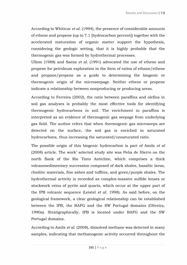
Results and Discussion | 7.0
165 | P a g e
According to Whiticar et al. (1994), the presence of considerable amounts
of ethene and propene (up to 7.1 [hydrocarbon percent]) together with the
accelerated maturation of organic matter support the hypothesis,
considering the geologic setting, that it is highly probable that the
thermogenic gas was formed by hydrothermal processes.
Ullom (1988) and Saenz et al. (1991) advocated the use of ethene and
propene for petroleum exploration in the form of ratios of ethane/ethene
and propane/propene as a guide to determining the biogenic or
thermogenic origin of the microseepage. Neither ethene or propene
indicate a relationship between nonproducing or producing areas.
According to Ferreira (2002), the ratio between paraffins and olefins in
soil gas analyses is probably the most effective tools for identifying
thermogenic hydrocarbons in soil. The enrichment in paraffins is
interpreted as an evidence of thermogenic gas seepage from underlying
gas field. The author refers that when thermogenic gas microseeps are
detected on the surface, the soil gas is enriched in saturated
hydrocarbons, thus increasing the saturated/unsaturated ratio.
The possible origin of this biogenic hydrocarbon is part of Amils et al
(2008) article. The work’ selected study site was Peña de Hierro on the
north flank of the Rio Tinto Anticline, which comprises a thick
volcanosedimentary succession composed of dark shales, basaltic lavas,
rhiolitic materials, fine ashes and tuffites, and green/purple shales. The
hydrothermal activity is recorded as complex-massive sulfide lenses or
stockwork veins of pyrite and quartz, which occur at the upper part of
the IPB volcanic sequence (Leistel et al. 1998). As said before, on the
geological framework, a clear geological relationship can be established
between the IPB, the BAFG and the SW Portugal domains (Oliveira,
1990a). Stratigraphically, IPB is located under BAFG and the SW
Portugal domains.
According to Amils et al. (2008), dissolved methane was detected in many
samples, indicating that methanogenic activity occurred throughout the
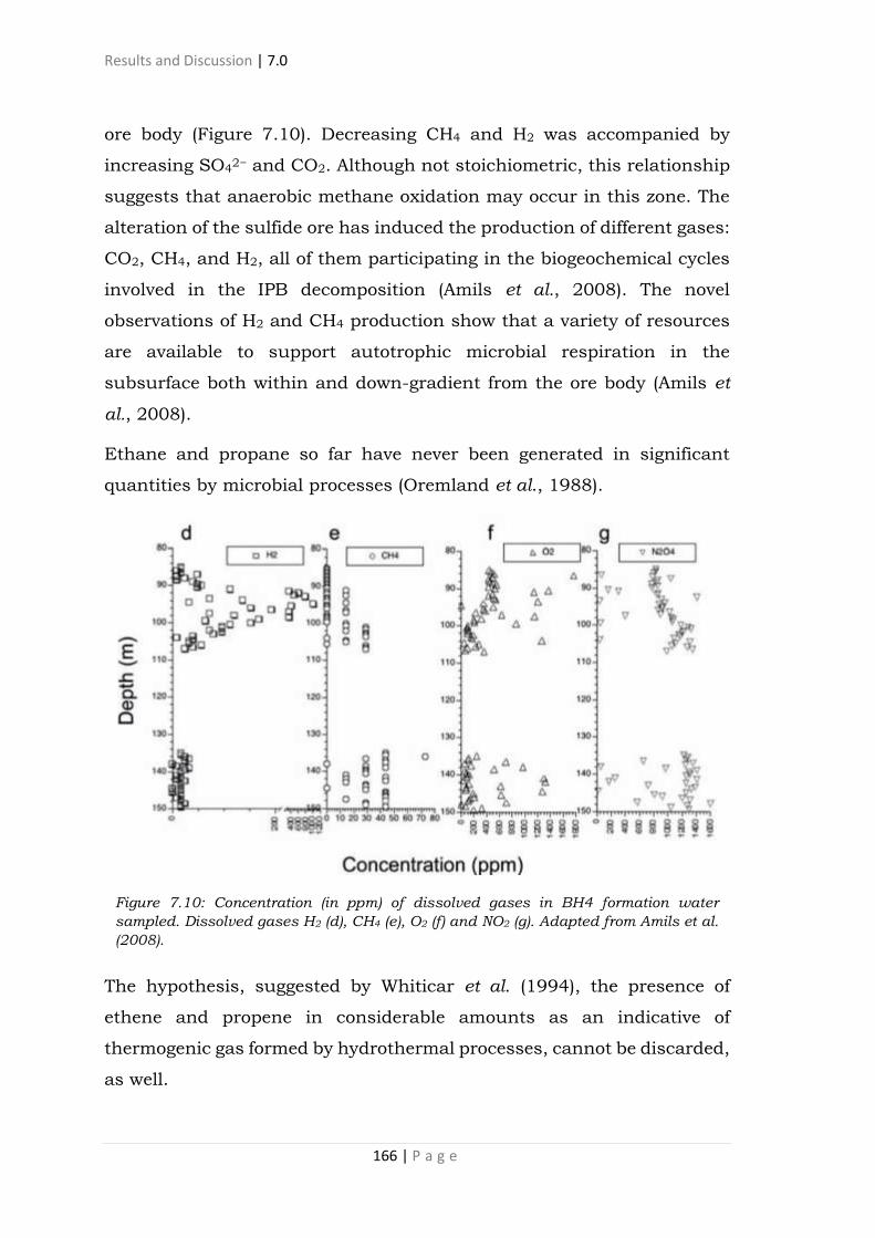
Results and Discussion | 7.0
166 | P a g e
ore body (Figure 7.10). Decreasing CH4 and H2 was accompanied by
increasing SO42− and CO2. Although not stoichiometric, this relationship
suggests that anaerobic methane oxidation may occur in this zone. The
alteration of the sulfide ore has induced the production of different gases:
CO2, CH4, and H2, all of them participating in the biogeochemical cycles
involved in the IPB decomposition (Amils et al., 2008). The novel
observations of H2 and CH4 production show that a variety of resources
are available to support autotrophic microbial respiration in the
subsurface both within and down-gradient from the ore body (Amils et
al., 2008).
Ethane and propane so far have never been generated in significant
quantities by microbial processes (Oremland et al., 1988).
The hypothesis, suggested by Whiticar et al. (1994), the presence of
ethene and propene in considerable amounts as an indicative of
thermogenic gas formed by hydrothermal processes, cannot be discarded,
as well.
Figure 7.10: Concentration (in ppm) of dissolved gases in BH4 formation water
sampled. Dissolved gases H2 (d), CH4 (e), O2 (f) and NO2 (g). Adapted from Amils et al.
(2008).

167 | P a g e
CONCLUSIONS, FINAL REMARKS, COST
EVALUATION AND FUTURE
PERSPECTIVES|8.0
Conclusions|8.1. . . . . . . . . . . . . . . . . . . . . . . . . . . . . . . . . . . . . . . . .167
Final Remarks|8.2. . . . . . . . . . . . . . . . . . . . . . . . . . . . . . . . . . . . . . . 169
Cost Evaluation|8.3. . . . . . . . . . . . . . . . . . . . . . . . . . . . . . . . . . . . . . 176
Future Perspectives|8.4. . . . . . . . . . . . . . . . . . . . . . . . . . . . . . . . . . . 177
Conclusions|8.1
he methodologies used to define the sampling areas (TN and HA)
proved to be very efficient to show possible hydrocarbon
emanations. However, the use of WV-2 images seems to be more
economically viable solution for obtaining radiometric data, considering
the high costs associated with the acquisition of airborne gamma-ray.
As verified in the map 2.1, the SPZ extends at least to the Spanish
territory (onshore and offshore) and also to the Portuguese offshore, thus
presenting a significant geographical extension. This information is
extremely important for a possible assessment of the economic evaluation
of hydrocarbon exploration in the region, not only for Portuguese, but
also for Spanish and maybe for Moroccan government.
From the geological prospecting point of view the presence of hydrocarbon
gases in SPZ formations is clear and evident. They are present in soil and
water, with significantly high levels, and the integration with TOC,
T

Conclusions, Final Remarks, Cost Evaluation and Future Perspectives | 8.0
168 | P a g e
vitrinite reflectance, rock-eval pyrolysis and GC-IRMS reveals the
presence of a senile unconventional petroleum system, with possible
interbedded of levels with different degrees of organic maturation (leading
to a mixture of thermogenic gases). The possible presence of biogenic
gases (ethene and propene) raises the hypothesis that Iberian Pyrite Belt
is located under the South Portuguese Zone.
It’s also important to note that, according to Skupio & Barberes (2017),
in the Paleozoic shales from Pomerania region (Poland) the hydrocarbons
are present above 3000 m depth. This information can provide an
estimative, by analogy, of how much deep the emanations can come from,
at SPZ.
The Mesozoic basins adjacent to the study area, the Algarve and the
Alentejo Basins (onshore and offshore), are composed by lithologies with
a porosity and permeability superior to those found in SPZ shales and
greywackes. Thus, a migration of any hydrocarbons fluids, from these
areas, is contrary to basic fluid dynamics. It’s also important to mention
that, according to the isotopic results present in this thesis and using the
relation between isotopic results and vitrinite reflectance, suggested by
Stahl et al. (1981) (figure 6.3), as a reference, the hydrocarbons found in
the SPZ formations represent a high maturity system. However,
according to Fernandes et al. (2013), the Mesozoic rocks of the Algarve
Basin lie within the oil window. Vitrinite reflectance ranges from 0.52-0.7
%Rr in the Lower Cretaceous to 1-1.1 %Rr in the Upper Triassic-
Hettangian. Miocene rocks that unconformably overlie the Mesozoic
strata are immature (0.42-0.47 %Rr). Thus, it’s difficult take these basins
as a possible source of this gases.
Currently, the Algarve and Alentejo regions (where the samples are
located) are very sensitive areas for the development of hydrocarbon
exploration projects. Society in general has constructed a negative image
of this activity based on misleading and sensationalist information,
beginning with the politicians. The research of the exploratory potential

Conclusions, Final Remarks, Cost Evaluation and Future Perspectives | 8.0
169 | P a g e
of a given region is not only an economic but also a political, social and
environmental issue (natural contamination of groundwater by
hydrocarbons, as seen in this project, is a good example). As previously
seen, water contaminated by toluene represents a serious concern to the
health of the locals (it is not yet known where the contamination is going
from a geographical point of view) and wells with high methane levels
represents a serious risk to the locals safety. The author and his advisers
informed the Portuguese authorities (environmental and health agencies)
about the contamination, once it was found.
Lastly, two water samples (W33 and W34) from two different boreholes
(few meters distance) contains worrying levels of CH4, from the safety
point of view. As said before, in the chapter 6, recommended action levels
for methane dissolved in water (Eltschlager et al., 2001), suggested that
when the level of methane gas is between 10 and 28 ppm monitoring is
required (warning, investigate) and immediate action is needed above 28
ppm. The sample W33 has a concentration of 12 ppm of CH4 and W34
contains 70 ppm, presenting a serious risk of borehole explosion (the
water is fully saturated with methane and the air is now flammable).
Considering the significant loss of methane (Parker & Britt, 2012;
Molofsky et al., 2016), as an inevitable consequence of the sampling
method, these values are the minimum content of the boreholes.
Final Remarks|8.2
The natural gas was introduced in Portugal in 1997 and between this
year and 2001 “gas works gas” was gradually replaced by gas in the
commercial/public service and residential sectors (Graph 8.1 and Table
8.2 [International Energy Agency, 2016a]).
According to International Energy Agency (2016b) report, in 2016 20% of
the electricity was generated by natural gas (52% of total electricity

Conclusions, Final Remarks, Cost Evaluation and Future Perspectives | 8.0
170 | P a g e
generation was made by fossil fuels) in this country (Graph 8.2). In the
same year, and according to the same report, Portugal imported 51.15%
of the gas from Algeria (Table 8.1 [International Energy Agency, 2016b]).
According to Eurostat (2015), in the year of 2013 Portuguese industry
consumed 70% of total gas in Portugal (Table 8.2). In this value,
consumed by the industry, just the non-metallic minerals industry (such
as glass, ceramic, cement, etc.) consumed 40%. Still according to the
same report, the industry consumed 35% of the electricity in Portugal, in
2013 (Table 8.2).
Eurostat (2016) highlights the development of electricity and natural gas
prices for both industrial and household users in the European Union
(EU); furthermore, price information for petroleum products is also
provided (Graphs 8.3, 8.4, 8.5 and 8.6 [Eurostat 2016]).
The price and reliability of energy supplies, electricity in particular, are
key elements in a country’s energy supply strategy (Eurostat 2016).
Electricity prices are of particular importance for international
competitiveness, as electricity usually represents a significant proportion
of total energy costs for industrial and service-providing businesses
(Eurostat 2016). In contrast to the price of some fossil fuels, which are
usually traded on global markets with relatively uniform prices, there is
a wider range of prices within the EU Member States for electricity or
natural gas (Eurostat, 2016). The price of electricity and natural gas is,
to some degree, influenced by the price of primary fuels and, more
recently, by the cost of carbon dioxide (CO2) emission certificates
(Eurostat, 2016).
In Portugal, the price of electricity and natural gas are among the highest
in European Union. The cost of electricity, for household consumers
(Graph 8.3), practiced in 2015 in Portugal was the 7º most expensive
price in EU (0.229 EUR/kWh) and for industry (Graph 8.4) was the 8º
most expensive (0.115 EUR/kWh) (Eurostat, 2016). The scenario is worse

Conclusions, Final Remarks, Cost Evaluation and Future Perspectives | 8.0
171 | P a g e
when we analyze the cost of gas in this country. In the same year,
Portugal practiced the 2º most expensive price in EU (0.098 EUR/kWh)
for household consumers (Graph 8.5) and the 4º most expensive (0.038
EUR/kWh) for industry (Graph 8.6 [Eurostat, 2016]). The basic prices
(without taxes and levies), for natural gas in Portugal, are the most
expensive practiced in EU (Graphs 8.5 and 8.6 [Eurostat, 2016]).
Unlike other parts of the world, natural gas and electricity transmission
networks in Europe are very well structured. As can be seen in the
European high voltage transmission grid (http://www.geni.org/global
energy/library/national_energy_grid/europe/europeannationalelectricity
grid.shtml [Global Energy Network Institute, 2017]) and the European
natural gas network (Map 8.1 [European Network of Transmission
System Operators for Gas, 2016]). These two maps demonstrate that the
production of natural gas and electricity in European territory can be
easily marketed across the whole continent.
Graph 8.1: Production and self-sufficiency of Portugal 2015. The blue bars represent
total primary energy supply (TPES- defined as energy production plus energy imports,
minus energy exports, minus international bunkers, then plus or minus stock changes).
Adapted from International Energy Agency (2016b).

Conclusions, Final Remarks, Cost Evaluation and Future Perspectives | 8.0
172 | P a g e
Portugal does not have significant proved reserves of natural gas. There
is no gas production in the national territory and, therefore, the country
depends on imports to supply all the domestic needs (International
Energy Agency, 2011). Barberes (2013) suggests that the exploration of
potential reserves of hydrocarbons in Portugal would mean a new stage
of energy production in Portugal and organic-rich shales, which appear
in various parts of the country, appear as hydrocarbon source/reservoirs
rocks (unconventional petroleum system).
Graph 8.2: Energy system transformation.
Adapted from International Energy Agency
(2016b).
Table 8.1: Energy security, main importers of
crude oil, oil products, natural gas and coal.
Adapted from International Energy Agency
(2016b).

Conclusions, Final Remarks, Cost Evaluation and Future Perspectives | 8.0
173 | P a g e
1973 1980 1990 2000 2005 2010 2013 2014 2015p
- - - - - - - - -
2267 6871 18503 30247 37623 25008 20764 20143 26641
- - - 94864 181102 209571 177377 161638 188515
- - - 30648 44478 48968 50404 49162 n/d
- - - 36773 60814 72775 72882 72000 n/d
Production of natural gas (Unit: TJ-gross)
Production of electricity from fossil fuels (Unit: GWh)
Net imports of natural gas (Unit: TJ-gross)
Final consumption of natural gas (Unit: TJ-gross)
Industry consumption of natural gas (Unit: TJ-gross)
Table 8.2: Production of natural gas, energy from fossil fuels, net imports of natural
gas, industry consumptions of natural gas and final consumption of natural gas,
between 1973-2015. Adapted from International Energy Agency (2016a).
Graph 8.3: Electricity prices for household consumers, second half 2015 (1)
(EUR/kWh). Adapted from Eurostat (2016).

Conclusions, Final Remarks, Cost Evaluation and Future Perspectives | 8.0
174 | P a g e
Graph 8.4: Electricity prices for industrial consumers, second half 2015 (1) (EUR/kWh).
Adapted from Eurostat (2016).
Map 8.1: The European natural gas
network (Portugal, Spain, France and
Switzerland) – Capacities at cross-
border points on the primary market.
The pipelines are represented by grey
lines. Adapted from European Network
of Transmission System Operators for
Gas (2016).
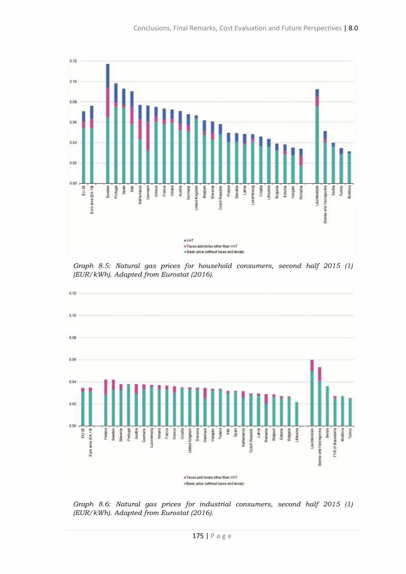
Conclusions, Final Remarks, Cost Evaluation and Future Perspectives | 8.0
175 | P a g e
Graph 8.6: Natural gas prices for industrial consumers, second half 2015 (1)
(EUR/kWh). Adapted from Eurostat (2016).
Graph 8.5: Natural gas prices for household consumers, second half 2015 (1)
(EUR/kWh). Adapted from Eurostat (2016).

Conclusions, Final Remarks, Cost Evaluation and Future Perspectives | 8.0
176 | P a g e
Cost Evaluation|8.3
Research is the foundation and fundamental driver of the creation of new
knowledge. Research requires investment, ongoing operational costs,
continual strategic thinking, and a firm appreciation of its value
(Stephens, 2013).
As said before, in the preface to this thesis, the values practiced in the
petroleum industry (sales, profits, investments, etc.) are equivalent to the
largest economies around the world. As one would expect, industrial
interest research has a high associated cost.
The industrial costs of the laboratory analyze performed in this project
are significantly high, ranging from US$ 40 per sample (TOC) to US$ 680
per sample (isotope). Therefore, the minimum industrial cost of the
results obtained in this work (laboratory analysis, satellite imagery and
airborne gamma ray) is around US$ 102,230 (taking into account the
prices practiced in the current market), which adds a high value to the
information contained herein.
The partnership with companies and laboratories made it possible to
carry out analyzes and obtain data with significantly reduced costs, thus
enabling the implementation of this project.
The results obtained using alternative (cheaper) methods appears as a
possibility for the viabilization of projects with high associated costs. This
becomes even more evident when we analyze the gamma radiation data
presented in this thesis.
The cost of airborne GR survey (usually associated with magnetic survey)
varies mainly depending on the country and the device (personal
communication). By airplane it ranges between US$ 4 per flight line km
(e.g., South Africa and Australia) and US$ 20 per flight line km (e.g., India
and Brazil); by helicopter it ranges between US$ 40 per flight line km
(e.g., South Africa and Australia) and US$ 80 per flight line km (e.g., India

Conclusions, Final Remarks, Cost Evaluation and Future Perspectives | 8.0
177 | P a g e
and Brazil). Using the AOI as an example (1,000 km2 with 75m of distance
between flight lines), the final cost varies between US$ 52,800-US$
264,000 (by airplane) and US$ 528,000-US$ 1,056,000 (by helicopter).
As mentioned earlier, the satellite images used in this study provide one
of the best resolutions among those available today. The average cost, per
square kilometer, of the WV2 images varies mainly if the product is
“archive” (8-Band Panchromatic + Multispectral: US$ 19 per sq. km) or
“new tasking” (8-Band Multispectral + Panchromatic: US$ 29 per sq. km)
(LANDinfo, 2016). For example, to cover all the AOI, the cost ranges
between US$ 19,000 and US$ 29,000 (1,000 km2).
The results presented in this thesis show that it is possible, at least
partially, to extract radiometric information from WV2 images. This could
imply a significant cost reduction, between 45% and 98.2% in radiometric
data acquisition, as it happened with the project to which this thesis
refers. Moreover, a satellite image can be acquired in a few hours and the
data processing can be done in a few days.
Future Perspectives|8.4
Economic development, when well managed by the political class, has the
natural consequence of social development, through the job creation,
development of infrastructure, etc. The knowledge (mapping) of the
natural resources is fundamental for the development of a solid
geostrategic policy, since Portugal, as said in the introduction of this
thesis, depends entirely on imports to supply its domestic demand for
hydrocarbons.
An interesting example of natural resources capitalization is the Parnaíba
complex of thermoelectric power plants (Brazil), administered by the
ENEVA company. Taking advantage of the privileged location, near the

Conclusions, Final Remarks, Cost Evaluation and Future Perspectives | 8.0
178 | P a g e
producing wells of natural gas, the plant has a high capacity of electric
generation at a low cost. In addition, 3,700 direct jobs are generated.
The next steps, after the publication of this project, demand greater
financial investments, mainly to increase the sampling grid (collection
and analysis of more samples) and to perform a seismic acquisition
campaigns. It is extremely important to evaluate the possible "paths"
used by hydrocarbons to the surface, and also to verify the potential
source levels of these hydrocarbons.
179 | P a g e
BIBLIOGRAPHY|9.0
Abad, I., Mata, M.P., Nieto, F., Velilla, N. 2001. The Phyllosilicates in
diagenetic-metamorphic rocks of the South Portuguese Zone,
southwestern Portugal. The Canadian Mineralogist, 39, pp. 1571-
1589, doi: 10.2113/gscanmin.39.6.1571.
Abad, I., Nieto, F., Velilla, N. 2002. Chemical and textural
characterization of diagenetic to low-grade metamorphic
phyllosilicates in turbidite sandstones of the South Portuguese
Zone: a comparison between metapelites and sandstones. Schweiz.
Mineral. Petrogr. Mitt., 82, pp. 303-324, doi: 10.5169/seals-62367.
Abrams, M.A. 2005. Significance of hydrocarbon seepage relative to
petroleum generation and entrapment. Marine and Petroleum
Geology, 22, pp. 457-477, doi: 10.1016/j.marpetgeo.2004.08.003.
Abrams, M.A. 2013. Best practices for the collection, analysis, and
interpretation of seabed geochemical samples to evaluate
subsurface hydrocarbon generation and entrapment. Offshore
Technology Conference, 24219, 21p., doi: 10.4043/24219-MS.
Abrams, M. A., Dahdah, N. 2011. Surface sediment hydrocarbons as
indicators of subsurface hydrocarbons – field calibration of existing
and new surface geochemistry methods in the Marco Polo Area Gulf
of Mexico. American Association Petroleum Geology Bulletin, 95
(11), pp. 1907-1935, doi: 10.1306/03211110130.
Abrams, M. A., Segall, M. P., Burtell, S. G. 2001. Best practices for
detecting, identifying, and characterizing near-surface migration of

Bibliography | 9.0
180 | P a g e
hydrocarbons within marine sediments. Offshore Technology
Conference, 13039, 14p., doi: 10.4043/13039-MS.
Al-Alfy, I.M., Nabih, M.A., Eysa, E.A. 2013. Gamma ray spectrometry logs
as a hydrocarbon indicator for clastic reservoir rocks in Egypt.
Applied Radiation and Isotopes, 73, pp. 90-95, doi:
10.1016/j.apradiso.2012.11.016.
Almeida-Filho, R., Miranda, F.P., Yamakawa, T. 1998. Remote detection
of a tonal anomaly in an area of hydrocarbon microseepage, Tucano
basin, north-eastern Brazil. International Journal of Remote
Sensing, 20 (13), pp. 2683-2688, doi: 10.1080/014311699212029.
Alpers, C.N., Dettman, D.L., Lohmann, K.C., Brabec, D. 1990. Stable
Isotopes of Carbon Dioxide in Soil Gas Over Massive Sulfide
Mineralization at Crandon, Wisconsin. Journal of Geochemical
Exploration, 38 (1-2), pp. 69-86, doi: 10.1016/0375-
6742(90)90093-p.
Amils, R., Fernández-Remolar, D., Gómez, F., González-Toril, E.,
Rodríguez, N., Briones, C., Prieto-Ballesteros, O., Sanz, J.L., Díaz,
E., Stevens, T.O., Stoker, C.R. 2008. Subsurface Geomicrobiology
of the Iberian Pyritic Belt. In: Dion, P. & Nautiyal, C.S. (eds.),
Microbiology of Extreme Soils. Soil Biology 13. Springer-Verlag
Berlin Heidelberg, pp. 205-223, doi: 10.1007/978-3-540-74231-9.
Aminzadeh F, Berge T, Connolly D, O’Brien G (eds.) 2013. Hydrocarbon
Seepage: from source to surface. AAPG/SEG Special Publication -
Geophysical Developments, 16, 256p, doi:
10.1190/1.9781560803119.
ARH Alentejo. 2011. Planos de Gestão das Bacias Hidrográficas
Integradas nas Regiões Hidrográficas 6 e 7 – Região Hidrográfica 6,
Volume I (Relatório), Parte 2 (Caracterização e Diagnóstico).
Ministério da Agricultura, Mar, Ambiente e Ordenamento do
Território, Portugal, 336p.

Bibliography | 9.0
181 | P a g e
Ashcroft, A.E. 1997. Ionization methods in organic mass spectrometry.
The Royal Society of Chemistry, UK, 176p, doi:
10.1039/9781847551191.
ATSDR. 2000. Toxicological profile for toluene. US Department of Health
and Human Services, Agency for Toxic Substances and Disease
Registry, USA.
B’Hymer, C. 2010. Headspace Sampling in GC. In: Cazes, J. (ed.),
Encyclopedia of Chromatography. CRC Press, USA, pp. 1050-1058,
doi: 10.1108/09504121011067166.
Bandeira de Mello, C.S., Françolin, J.B.L., Miller, D.J., Gonçalves, R.C.S.,
Capilla, R., Lopes, J.P., Jesuíno, L.S., Silva Freitas, L.C., Soares
Filho, J.R.S., Fontes, R.A. 2007. Principais metodologias de
prospecção geoquímica de hidrocarbonetos em superfície. In: Licht,
O.A.B., Bandeira de Mello, C.S. & Silva C.R. (eds.), Prospecção
Geoquímica de Depósitos Minerais Metálicos, Não-Metálicos, Óleo
e Gás. Rio de Janeiro, SBGq, CPRM, 788p.
Barberes, G.A. 2013. A utilização da espectrometria de raios gama na
exploração de shale gas - Caso do carbonífero da Zona Sul
Portuguesa. M.Sc. Thesis, University of Coimbra, 110p.
(unpublished).
Barberes, G.A., Fonseca, P.E., Pena dos Reis, R., Pimentel, N., Azevedo,
M. 2014a. Preliminary assessment of potential for Shale Gas in
South Portuguese Zone carboniferous units. Comunicações
Geológicas, 101 (II), pp. 737-741.
Barberes, G.A., Karcz, P., Pena dos Reis, R., Pimentel, N., Fonseca, P.E.,
Azevedo, M. 2015. Organic geochemical results from the shales of
the South Portuguese Zone, southern Portugal. AAPG
Datapages/Search and Discovery, Article #90226, Lisbon,
Portugal, Book of Abstracts.

Bibliography | 9.0
182 | P a g e
Barberes, G.A., Pena dos Reis, R., Pimentel, N., Fonseca, P.E., Azevedo,
M. 2014b. Application of Thorium-Normalized method to identify
any hydrocarbons anomalies in South Portuguese Zone
Carboniferous units. Comunicações Geológicas, 101 (II), pp. 743-
746.
Barberes, G.A., Pena dos Reis, R., Spigolon, A.L.D., Fonseca, P.E.,
Bandeira de Mello, C., Barata, M.T. 2018. Groundwater Natural
Contamination by Toluene in Beja and Faro Districts, Portugal.
Geosciences, 8 (1), 9, doi:10.3390/geosciences8010009.
Bernard, B.B., Brooks, J.M., Sacket, W.M. 1978. Light hydrocarbons in
recent Texas continental shelf and slope sediments. Journal of
Geophysical Research, 83, pp. 4053-4061, doi:
10.1029/jc083ic08p04053.
Berge, T.B. 2011. Recognition and Meaning of Hydrocarbon Seeps. AAPG
Search and Discovery, Article #40759.
B.F. Environmental Consultants Inc. 2012. Methane Gas Migration and
Your Water Well – A Pennsylvania Perspective. B.F. Environmental
Consultants Inc., 2p.
Boyer, C., Clark, B. 2011. Shale Gas: A Global Resource. OilField Review,
23 (3), pp. 28-39.
Boyle, R.W. 1982. Geochemical prospecting for thorium and uranium
deposits. Elsevier Publishing Company, 498p.
Brandon Weil, A., Gutiérrez-Alonso, G., Johnston, S.T., Pastor-Galán, D.
2013. Kinematic constraints on buckling a lithospheric-scale
orocline along the northern margin of Gondwana: A geologic
synthesis. Tectonophysics, 582, pp. 25-49, doi:
10.1016/j.tecto.2012.10.006.
Bibliography | 9.0
183 | P a g e
Brown, A. 2000. Evaluation of possible gas microseepage mechanisms.
AAPG Bulletin, 84 (11), pp. 1775-1789, doi: 10.1306/8626C389-
173B-11D7-8645000102C1865D.
Burtell, S.G., Jones III, V.T. 1996. Exploration benzene content of
subsurface brines can indicate proximity of oil, gas. Oil & Gas
Journal Newsletter (http://www.ogj.com/articles/print/volume-
94/issue-23/in-this-issue/exploration/exploration-benzene-
content-of-subsurface-brines-can-indicate-proximity-of-oil-
gas.html).
Cerqueira, J.R., Santos Neto, E.V.; Takaki, T, Prinzhofer, A. 1999.
Ocorrência de hidrocarbonetos de diferentes origens num mesmo
sistema de reservatórios na parte centro-sul da Bacia do Paraná.
Congresso de Geoquímica dos países de língua portuguesa,
Congresso Brasileiro de Geoquímica, Anais da Sociedade Brasileira
de Geoquímica, pp. 383-388.
Chafin, D.T., Swanson, D.M., Grey, D.W. 1996. Methane-Concentration
and Methane-Isotope Data for Ground Water and Soil Gas in the
Animas River Valley, Colorado and New Mexico, 1990-91. U.S.
Geological Survey. Water Resources Investigation Report 93-4007,
49p.
Clarke, R.H., Cleverly, R.W. 1991. Leakage and post-accumulation
migration. In: England, W.A. & Fleet, A.J. (eds.), Petroleum
migration. Geological Society Special Publication, London, 59, pp.
265-271.
Clark, P.E., Rilee, M.L. 2010. Remote sensing tools for exploration-
Observing and interpreting the electromagnetic spectrum.
Springer, 343p., doi 10.1007/978-1-4419-6830-2.
Cline, J.D., Holmes, M.L. 1977. Submarine seepage of natural gas in
Norton Sound, Alaska. Science, 198, pp. 1149-1153, doi:
10.1126/science.198.4322.1149.

Bibliography | 9.0
184 | P a g e
Collins, A.G. 1975. Geochemistry of OilField Waters. Elsevier,
Amsterdam, 496p, doi: 10.1016/s0376-7361(08)x7011-6.
Collins, W., Raines, G.L., Canney, F.C. 1978. Airborne spectroradiometer
detection of heavy-metal stress in vegetation canopies; Prog, and
Abstracts 5th Internat. Assoc. Genesis Ore Deposits, Snowbird,
Utah, 74p.
Conrad, R. 1996. Soil microorganisms as controllers of atmospheric trace
gases (H2, CO, CH4, OCS, N2O, and NO). Microbiological Reviews,
American Society for Microbiology, pp. 609–640.
Czaja, W., Manning, B., McLean, L., Murphy, J.M. 2015. Fusion of aerial
gamma ray survey and remote sensing data for a deeper
understanding of radionuclide fate after radiological incidents:
examples from the fukushima dai-ichi response. Journal of
Radioanalytical and Nuclear Chemistry, 307 (3), pp. 2397-2401,
doi: 10.1007/s10967-015-4650-z.
Deines, P. 1980. The isotopic composition of reduced organic carbon. In:
Fritz, P. & Fontes, J.Ch. (eds.), Handbook of Environmental Isotope
Geochemistry. The Terrestrial Environment, 1, Elsevier,
Amsterdam, pp. 329-406.
Días-del-Río, V., Somoza, L., Martínez-Frias, J., Mata, M.P., Delgado, A.,
Hernandez-Molina, F.J., Lunar, R., Martín.Rubi, J.A., Maestro, A.,
Fernández-Puga, M.C., León, R., Llave, E., Medialdea, T., Vázquez,
J.T. 2003. Vast fields of hydrocarbon-derived carbonate chimneys
related to the accretionary wedge/olistostrome of the Gulf of Cádiz.
Marine Geology, 195, pp. 177-200, doi: 10.1016/s0025-
3227(02)00687-4.
Dias, R., Ribeiro, A., 1993. Porto-Tomar Shear Zone, a major structure
since the beginning of the Hercynian Orogeny. Terra Abstracts
supplement number 6 to Terra Nova 5, 11.

Bibliography | 9.0
185 | P a g e
Dias, R., Ribeiro, A. 1995. The Ibero-Armorican Arc: A collision effect
against an irregular continent? Tectonophysics, 246, pp. 113-128,
doi: 10.1016/0040-1951(94)00253-6.
Dias, R., Ribeiro, A., Romão, J., Coke, C., Moreira, N. 2016. A review of
the arcuate structures in the Iberian Variscides; constraints and
genetic models. Tectonophysics, 681, pp. 170-194, doi:
10.1016/j.tecto.2016.04.011.
DigitalGlobe 2016. WorldView-2 data sheet,
http://global.digitalglobe.com/sites/default/
files/DG_WorldView2_DS_PROD.pdf (accessed May, 2016).
El-Sadek, M.A. 2002. Application of thorium-normalized airborne radio-
spectrometric survey data of Wadi Araba area, North-eastern
Desert, Egypt, as a guide to the recognition of probable subsurface
petroleum accumulations. Applied Radiation and Isotopes, 57, pp.
121-130, doi: 10.1016/s0969-8043(02)00082-9.
Eltschlager, K.K., Hawkins, J.W., Ehler, W.C., Baldassare, F. 2001.
Technical measures for the investigation and mitigation of fugitive
methane hazards in areas of coal mining. U.S. Department of the
Interior – Office of Surface Mining. Pittsburgh, PA, 124p.
Etiope, G. 1998. Transport of radioactive and toxic matter by gas
microbubbles in the ground. J. Environ. Radioactivity, 40 (1), pp.
11-13, doi: 10.1016/s0265-931x(97)00068-4.
Etiope, G. 2004. New Directions: GEM—Geologic Emissions of Methane,
the missing source in the atmospheric methane budget.
Atmospheric Environment, 38, pp. 3099-3100, doi:
10.1016/j.atmosenv.2004.04.002.
Etiope, G. 2005. Mud volcanoes and microseepage: the forgotten
geophysical components of atmospheric methane budget. Ann
Geophys, 48, pp. 1-7, doi: 10.4401/ag-3175.

Bibliography | 9.0
186 | P a g e
Etiope, G. 2009a. A global dataset of onshore gas and oil seeps: a new
tool for hydrocarbon exploration. Oil and Gas Business, 10p.
Etiope, G. 2009b. GLOGOS, A New Global Onshore Gas-Oil Seeps
Dataset. AAPG Search and Discovery, Article #70071.
Etiope, G. 2009c. Natural emissions of methane from geological seepage
in Europe. Atmospheric Environment, 43, pp. 1430-1443, doi:
10.1016/j.atmosenv.2008.03.014.
Etiope, G. 2015. Natural gas seepage-The earth’s hydrocarbon degassing.
Springer, Switzerland. 199p, doi: 10.1007/978-3-319-14601-0.
Etiope, G., Klusman, R.W. 2002. Geologic emissions of methane to the
atmosphere. Chemosphere, 49, pp. 777-789, doi: 10.1016/s0045-
6535(02)00380-6.
Etiope, G, Klusman, R.W. 2010. Microseepage in drylands: flux and
implications in the global atmospheric source/sink budget of
methane. Glob. Plan. Change, 72, pp. 265-274, doi:
10.1016/j.gloplacha.2010.01.002.
Etiope, G., Lombardi, S. 1996. Laboratory simulation of geogas
microbubble flow. Environ. Geol, 27, pp. 226-232, doi:
10.1007/bf00770436.
European Network of Transmission System Operators for Gas. 2016. The
European Natural Gas Network 2016 – Capacities at Cross-Border
Points on the Primary Market.
http://www.entsog.eu/public/uploads/files/maps/transmissionc
apacity/2016/ENTSOG_CAP_MAY2016_A0FORMAT.pdf (accessed
January, 2017)
Eurostat. 2015. Energy balance sheets - 2013 data. Eurostat Statistical
books. ISSN 1830-7558, 84p.

Bibliography | 9.0
187 | P a g e
Eurostat. 2016. Energy price statistics - Statistics Explained.
http://epp.eurostat.ec.europa.eu/statisticsexplained/ (accessed
January, 2017).
Fernandes, P., Rodrigues, B., Borges, M., Matos, V., Clayton, G. 2013.
Organic maturation of the Algarve Basin (southern Portugal) and
its bearing on thermal history and hydrocarbon exploration.
Marine and Petroleum Geology, 46, pp. 210-233, doi:
10.1016/j.marpetgeo.2013.06.015.
Fernandes, P., Musgrave, J.A., Clayton, G., Pereira, Z., Oliveira, J.T.,
Goodhue, R., Rodrigues, B. 2012. New evidence concerning the
thermal history of Devonian and Carboniferous rocks in the South
Portuguese Zone. Journal of the Geological Society of London, 169,
pp. 647-654, doi: 10.1144/jgs2011-156.
Ferreira, J.C. 2002. Light Hydrocarbons in Soil Underlain by Exclusively
Crystalline Rocks and in Sedimentary Basins: Exploratory
Implications. Revista Latino Americana de Geochímica Orgânica, 6,
pp. 31-39.
Fertl, W.H. 1979. Gamma ray spectral data assists in complex formation
evaluation. Society of Petrophysicists and Well-Log Analysts, 20,
pp. 3-37.
Figueiras, J., Mateus, A., Gonçalves, M.A., Waerenborgh, J., Fonseca, P.
2002. Geodynamic evolution of the South Variscan Iberian Suture
as recorded by mineral transformations. Geodinamica Acta, 15
(2002), pp. 45-61, doi: 10.1080/09853111.2002.10510738.
Fonseca, P., Ribeiro, A. 1993. Tectonics of Beja-Acebuches Ophiolite: a
major suture in the Iberian Variscan Foldbelt. Geol. Rundsch.
Springer, 82, pp. 440-447, doi: 10.1007/bf00212408.
Fonseca, P., Munhá, J., Pedro, J., Rosas, F., Moita, P., Araújo, A., Leal,
N. 1999. Variscan Ophiolites and high-pressure metamorphism in
southern Iberia. Ofioliti, 24 (2), pp. 259-268.

Bibliography | 9.0
188 | P a g e
Fonseca, P.E., Pimentel, N., Pena dos Reis, R., Barberes, G.A. 2015.
Carboniferous Black-Sahles and Shale-Gas Potential in
Southwestern Portugal. Post-Conference Field-trip. 20th-21st May
2015, 1st ed., AAPG – Europe Region Annual Conference &
Exhibition, Lisbon, Portugal.
Fontana, J.V. 2000. Soil Gas Monitoring Activities near the Southeastern
Boundary of the Leyden Gas Storage Facility, Leyden Colorado.
ESN Rocky Mountain – Environmental Services Network. ESN
Project, 0126, 28p.
Freitas, J.G., Fletcher, B., Aravena, R., Barker, J.F. 2010. Methane
Production and Isotopic Fingerprinting in Ethanol Fuel
Contaminated Sites. Ground Water, 48 (6), pp. 844-857, doi:
10.1111/j.1745-6584.2009.00665.x.
Friedman, G.M., Sanders, J.E. 1978. Principles of Sedimentology. John
Wiley & Sons, Inc., New York, 792p.
Geosoft 2005. Montaj 256-Channel Radiometrics Processing.
Radiometric processing extension for Oasis Montaj v6.1. User
Guide and Tutotial. Geosoft Knowlodge from Data, 43p.
Gilbert, D., Woodruff, C., Preston, A., Thomas, R., Wood, M. 1983.
Exposure and Risk Assessment for Toluene. PB8S-221505.
National Technical Information Service, Springfield, VA, 182p.
Global Energy Network Institute. 2017. European high voltage
transmission grid.
http://www.geni.org/globalenergy/library/national_energy_grid/
europe/europeannationalelectricitygrid.shtml (accessed April,
2017).
Gomez-Belinchon, J.I., Grimalt, J.O. 1991. Volatile organic compounds
in two polluted rivers in Barcelona (Catalonia, Spain). Water
Research, 25, pp. 577-589, doi: 10.1016/0043-1354(91)90130-i.

Bibliography | 9.0
189 | P a g e
Government of Canada. 1992. Toluene - Priority Substances List
Assessment Report Nº 4. Canadian Environmental Protection Act.
Canada Communication Group, Publishing, 26p.
Grob, R.L. 2004. Theory of Gas Chromatography. In: Grob, R.L. & Barry,
E.F. (eds.) Modern practice of gas chromatography. John Wiley &
Sons, USA, pp. 25-64, doi: 10.1002/0471651141.
Ground Water Protection Council and All Consulting. 2009. Modern
Shale Gas Development in the United States: A Primer.
Washington, DC, US Department of Energy Office and Fossil
Energy and National Energy Technology Laboratory.
Gülensoy, N.; Alvarez, P.J.J. 1999. Diversity and correlation of specific
aromatic hydrocarbon biodegradation capabilities. Biodegradation,
10, 331–340.
Hale, M. 2000. Genesis, behaviour and detection of gases in the crust.
In: Govett, G.J.S. (ed.) Handbook of exploration geochemistry
volume 7 - Geochemical Remote Sensing of the Sub-Surface.
Elsevier, The Netherlands, pp. 3-16.
Hemphill, W.R., Watson, R.D., Bigelow, R.C., Hessen, T.D. 1977.
Measurement of luminescence of geochemically stressed trees and
other materials. U.S. Geol. Surv. Prof. Paper, 1015, pp. 93-112.
Holmes, A.J., Roslev, P., Mcdonald, I.R., Iversen, N., Henriksen, K.,
Murrell, J.C. 1999. Characterization of methanotrophic bacterial
populations in soils showing atmospheric methane uptake. Applied
and Environmental Microbiology, American Society for
Microbiology, 65 (8), pp. 3312-331, pmid: 10427012.
Horsfield, B., Rullkotter, J. 1994. Diagenesis, Catagenesis and
Metagenesis of Organic Matter. In: Magoon, L.B. & Dow, W.G.
(eds.), The Petroleum System - from Source to Trap. AAPG Memoir,
United States of America, pp. 189-200, doi: 10.1306/M60585C10.

Bibliography | 9.0
190 | P a g e
Hovland, M., Jensen, S., Fichler, C. 2012. Methane and minor oil macro-
seep system - their complexity and environmental significance.
Mar. Geol., pp. 332-334 and 163-173, doi:
10.1016/j.margeo.2012.02.014.
Hunt, J.M. 1996. Petroleum geochemistry and geology. W.H. Freeman
and Co, New York, 743p.
International Energy Agency. 2016a. World Energy Statistics.
OECD/IEA, 789p.
International Energy Agency. 2016b. Portugal - Energy System Overview.
IEA-Energy Balance, 1p.
International Energy Agency. 2011. Oil & Gas Security Emergency
Response of IEA Countries, Portugal. OECD/IEA,
http://www.iea.org/publications/freepublications/publication/po
rtugal_20 11.pdf. (accessed April, 2013).
Isotech. 2014. Procedure for taking cuttings samples in IsoJars®. Isotech
Laboratories Inc., USA, 1p. (available in:
http://www.isotechlabs.com/products/other/isojars.html).
James, A.T. 1983. Correlation of natural gas by use of carbon isotopic
distribution between hydrocarbon components. AAPG Bulletin, 67,
pp. 1176-1191, doi: 10.1306/03B5B722-16D1-11D7-
8645000102C1865D.
Jones, V.T., Drozd, R.J. 1983. Prediction of oil or gas potential by near-
surface geochemistry. AAPG Bulletin, 67, pp. 932-952, doi:
10.1306/03B59AA8-16D1-11D7-8645000102C1865D.
Jorge, R.C.G.S., Fernandes, P., Rodrigues, B., Pereira, Z., Oliveira, J.T.
2013. Geochemistry and provenance of the Carboniferous Baixo
Alentejo Flysch Group, South Portuguese Zone. Sedimentary
Geology, 284-285, pp. 133-148, doi:
10.1016/j.sedgeo.2012.12.005.
Bibliography | 9.0
191 | P a g e
Kappel, W.M., Nystrom, E.A. 2012. Dissolved Methane in New York
Groundwater. U.S. Geological Survey, Open-file Report 2012-1162,
6p.
Kisch, H.J. 1987. Correlation between indicators of very low-grade
metamorphism. In: Frey, M. (ed.), Low-Temperature
Metamorphism. Blackie and Son, London, pp. 227-300.
Khan, S.D., Jacobson, S. 2008. Remote sensing and geochemistry for
detecting hydrocarbon microseepages. GSA Bull., 120, 96-105, doi:
10.1130/0016-7606(2008)120[96:RSAGFD]2.0.CO;2.
Kirk, R.E., Othmer, D.F., Grayson, M., Eckroth, D. 2004. Kirk-Othmer
Encyclopedia of Chemical Technology. John Wiley, New York, 5th
Edition, 22950p, doi: 10.1002/0471238961.
Klusman, R.W. 2003. Rate measurements and detection of gas
microseepage to the atmosphere from an enhanced oil
recovery/sequestration project, Rangely, Colorado, USA. Applied
Geochemistry, 18, pp. 1825–1838, doi: 10.1016/s0883-
2927(03)00108-2.
Klusman, R.W., Saeed, M.A. 1996. Comparison of light hydrocarbon
microseepage mechanisms. In: Schumacher, D. & Abrams, M.A.
(eds.), Hydrocarbon Migration and Its Near-Surface Expression
Amer. Assoc. Petrol. Geol. Memoir 66, Tulsa, OK, pp. 157-168, doi:
10.1306/M66606C12.
Kolb, B, Ettre, L.S. 2006. Static headspace-gas chromatography – theory
and practice. Wiley-Interscience, USA, 349p.
Korn, D. 1997. The Palaeozoic ammonoids of the South Portuguese Zone.
Memórias do Instituto Geológico e Mineiro, 33, 131p.
Kostakis, K., Harrison, J.P. 1999. Numerical analysis of gasbubble flow
in water-filled natural fractures. Comput. Geosci., 24, pp. 3-28,
doi: 10.1016/S0266-352X(98)00027-5.

Bibliography | 9.0
192 | P a g e
Kristiansson, K. Malmqvist, L. 1982. Evidence for non-diffusive transport
of 222Rn in the ground and a new geophysical model for the
transport. Geophysics, 47, pp. 1444-1452, doi:
10.1190/1.1441293.
Kübler, B. 1967. La cristallinité de l’illite et les zones tout à fait
supérieures de métamorphisme. In: Schaer J.P. (ed.), Étages
tectoniques: colloque Neuchâtel 1966. A La Baconniere, Neuchâtel,
pp. 105-122.
LANDinfo Worldwide Mapping LLC 2016. Buying Satellite Imagery:
Pricing Information for High Resolution Satellite Imagery,
http://www.landinfo.com/satellite-imagery-pricing.html (accessed
May, 2016).
Law, B.E., Curtis, J.B. 2002. Introduction to Unconventional Petroleum
Systems. AAPG Bulletin, 86 (11), pp. 1851–1852, doi:
10.1306/61eedda0-173e-11d7-8645000102c1865d.
Lawrence, S.J. 2006. Description, Properties, and Degradation of
Selected Volatile Organic Compounds Detected in Ground Water -
A Review of Selected Literature. Department of the Interior, U.S.
Geological Survey, USA. 54p.
Lefort, J.P. 1989. Basement Correlation Across the North Atlantic.
Springer-Verlag, Berlin, 148p, doi: 10.1007/978-3-642-73350-5.
Leistel, J.M., Marcoux, E., Theiblemont, D., Quesada, C., Sanchez, A.,
Almodovar, G.R., Pascual, E., Saez, R. 1998. The volcanic-hosted
massive sulphide deposits of the Iberian Pyrite Belt. Mineralium
Deposita, 33, pp. 2-30, doi: 10.1007/s001260050130.
Leusch, F., Bartkow, M. 2010. A short primer on benzene, toluene,
ethylbenzene and xylenes (BTEX) in the environment and in
hydraulic fracturing fluids. Griffity University Press. 8p.

Bibliography | 9.0
193 | P a g e
Levine, J.R., Davis, A. 1989. The relationship of coal optical fabrics to the
Alleghanian tectonic deformation in the central Appalachian
foldand- thrust belt, Pennsylvania. Geological Society of America
Bulletin, 101 (10), pp. 1333-1347, doi: 10.1130/0016-
7606(1989)101<1333:TROCOF>2.3.CO;2.
Li, H., Carlson, K.H. 2014. Distribution and Origin of Groundwater
Methane in the Wattenberg Oil and Gas Field of Northern Colorado.
Environ. Sci. Technol., 48, pp. 1484−1491, doi:
dx.doi.org/10.1021/es404668b.
Link, W.K. 1952. Significance of oil and gas seeps in world oil exploration.
AAPG Bulletin, 36, pp. 1505-1540.
Loch, J.P.G., van Dijk-Looyaard, A., Zoeteman, B.C.J. 1989. Organics in
groundwater. In: Wheeler, D., Richardson, M. L. & Bridges, J.
(eds.), The Future for Water Quality in Europe. Pergamon Press,
UK. pp: 39-55.
Lowrie, A., Hamiter, R., Mo¡ett, S., Somoza, L., Maestro, A., Lerche, I.
1999. Potential pressure compartments sub-salt in the Gulf of
Mexico and beneath massive debris £ows in the Gulf of Cadiz. Final
Proc. 19th Conf. GCSSEPM Advanced Reservoir Characterization,
Houston, TX, USA, pp. 271-280.
Macgregor, D.S. 1993. Relationships between seepage, tectonics and
subsurface petroleum reserves. Marine and Petroleum Geology, 10,
pp. 606-619, doi: 10.1016/0264-8172(93)90063-X.
Madhavi, T., Mani, D., Lakshmi, M., Kalpana, G., Patil, D.J., Dayal, A.M.
2008. Surface Geochemical Studies for Light Gaseous
Hydrocarbons: Findings from Recent Gas Seepages in Anantapur,
Andhra Pradesh. 7th International Conference & Exposition on
Petroleum Geophysics, P-285, 3p.
Maier, U., Mayer, U., Crathwohl, P. 2005. Natural Attenuation of Volatile
Hydrocarbons in the Unsaturated Zone – modeling for the Vaerlose

Bibliography | 9.0
194 | P a g e
field site. In: Thomson, N.R. (ed.), Bringing Groundwater Quality
Research to the Watershed Scale. Proceedings of CG2004, the 4th
International Groundwater Quality Conference, Canada, IAHS
Publi., 297p.
Magoon, L.B., Dow, W.G. 1994, The Petroleum System. In: Magoon, L.B.
& Dow, W.G. (eds.), The petroleum system: From source to trap:
AAPG Memoir 60, 34p.
Magoon L.B., Schmoker, J.W. 2000. The total petroleum system - the
natural fluid network that constraints the assessment units. U.S.
Geological Survey World Petroleum Assessment 2000, description
and results: USGS digital data series 60. World Energy Assessment
team, 31p.
Malmqvist, L., Kristiansson, K. 1984. Experimental evidence for an
ascending microflow of geogas in the ground. Earth and Planetary
Science Letters, 70, pp. 407-416, doi: 10.1016/0012-
821X(84)90024-4.
Malmqvist, L., Kristiansson, K. 1985. A physical mechanism for the
release of free gases in the lithosphere. Geoexploration, 23, pp.
447-453, doi: 10.1016/0016-7142(85)90072-9.
Maldonado, A., Somoza, L., Pallarés, L. 1999. The Betic orogen and the
Iberian–African boundary in the Gulf of Cadiz: geological evolution
(central North Atlantic). Marine Geology, 155, pp. 9-43, doi:
10.1016/S0025-3227(98)00139-X.
Mantero, E.M., Alonso-Chaves, F.M., García-Navarro, E., Azor, A. 2011.
Tectonic style and structural analysis of the Puebla de Guzmán
Antiform (Iberian Pyrite Belt, South Portuguese Zone, SW Spain).
In: Poblet, J. & Lisle R.J. (eds.), Kinematic Evolution and Structural
Styles of Fold-and-Thrust Belts. The Geological Society of London,
Geological Society Special Publication, 349, pp. 203-222, doi:
10.1144/SP349.11.

Bibliography | 9.0
195 | P a g e
Mateus, A., Figueiras, J., Gonçalves, M., Fonseca, P. 1999. Evolving fluid
circulation within the variscan Beja-Acebuches Ophiolite complex
(SE, Portugal). Ofioliti, 24 (2), pp. 269-282.
Matte, P. 1986. Tectonics and plate tectonic model for the variscan belt
of Europe. Tectonophysics, 126, pp. 329-374, doi: 10.1016/0040-
1951(86)90237-4.
Matthews, M.D. 1996. Migration - A view from the top. In: Schumacher,
D. & Abrams, M.A. (eds.), Hydrocarbon Migration and Its Near-
Surface Expression. Amer. Assoc. Petrol. Geol. Memoir 66, Tulsa,
OK, pp. 139–155, doi: 10.1306/M66606C11.
McAuliffe, C. 1963. Solubility in water of Cl-C9 hydrocarbons. Nature,
200, pp. 1092-1093, doi: 10.1038/2001092a0.
McCormack, N., Clayton, G., Fernandes, P. 2007. The thermal history of
the Upper Palaeozoic rocks of southern Portugal. Marine and
Petroleum Geology, 24, pp. 145-150, doi:
10.1016/j.marpetgeo.2007.01.002.
McGraw-Hill (ed.) 2003. Dictionary of Chemistry, 2nd edition. McGraw-
Hill, USA, 431p, doi: 10.1036/0071417974.
McNair, H.M, Miller, J.M. 2009. Basic gas chromatography. John Wiley
& Sons, USA, 239p.
Mendez, A., Bruzual, J. 2003. Molecular characterization of petroleum
and its fractions by mass spectrometry. In: Hsu, C.S. (ed.),
Analytical advances for hydrocarbon research. Springer, USA, pp.
73-94, doi: 10.1007/978-1-4419-9212-3.
Merian, E., Zander, M. 1982. Volatile aromatics. In: Hutzinger O, (ed.),
Handbook of environmental chemistry. 3 (B), Anthropogenic
compounds, Berlin, Springer, pp. 117-161.
Merriman, R.J., Peacor, D.R. 1999. Very low-grade metapelites:
mineralogy, microfabrics and measuring reaction progress. In:
Bibliography | 9.0
196 | P a g e
Frey, M. & Robinson, D. (eds.), Low Grade-Metamorphism.
Blackwell Science, Oxford, pp. 10-60.
Miller, J.M. 2005. Chromatography: concepts and contrasts. John Wiley
& Sons, USA. 490p.
Moldoveanu, S.C., David, V. 2002. Sample preparation in
chromatography. Elsevier, The Netherlands, 930p.
Molofsky, L.J., Connor, J.A., Wylie, A.S., Wagner, T., Farhat, S.K. 2013.
Evaluation of Methane Sources in Groundwater in Northeastern
Pennsylvania. Groundwater, 51 (3), pp. 333-349, doi:
10.1111/gwat.12056.
Molofsky, L.J., Richardson, S.D., Gorody, A.W., Baldassare, F., Black,
J.A., McHugh, T.E., Connor, J.A. 2016. Effect of Different Sampling
Methodologies on Measured Methane Concentrations in
Groundwater Samples. Groundwater, 54 (5), pp. 669-680, doi:
10.1111/gwat.12415.
Moreno, C., González, F. 2004. Estatigrafía - Zona Sudportuguesa. In:
J.A. Vera (ed.), Geología de España. SGE-IGME, Spain, pp. 201-
204.
Mudelsee, M. 2003. Estimating Pearson’s correlation coefficient with
bootstrap confidence interval from serially dependent time series.
Mathematical Geology, 35 (6), doi:
10.1023/b:matg.0000002982.52104.02.
Munhá, J. 1990. Metamorphic Evolution of the South Portuguese/Pulo
Do Lobo Zone. In: Dallmeyer, R.D. & Martínez García, E. (eds.), Pre-
Mesozoic Geology of Iberia. Springer-Verlag, Berlin, pp. 363-368,
doi: 10.1007/978-3-642-83980-1.
Naftz, D.L., Hadley, H.K., Hunt, G.L. 1998. Determination of Methane
Concentrations in Shallow Ground Water and Soil Gas near Price,
Utah. U.S. Geological Survey. ES-191-97, 4p.

Bibliography | 9.0
197 | P a g e
Oliveira, J.T. 1983. The marine Carboniferous of South Portugal: a
stratigraphic and sedimentological approach. In: Lemos de Sousa,
M.J. & Oliveira, J.T. (eds.). The Carboniferous of Portugal. Mem.
Serv. Geol. Portugal, 29, pp. 3-37.
Oliveira, J.T. 1990a. Metamorphic Evolution of the South
Portuguese/Pulo Do Lobo Zone. In: Dallmeyer, R.D. & Martínez
García, E. (eds.), Pre-Mesozoic Geology of Iberia. Springer-Verlag,
Berlin, pp. 363-368, doi: 10.1007/978-3-642-83980-1.
Oliveira, J.T. 1990b. Stratigraphy and syn-sedimentary tectonism in the
South Portuguese Zone. In: Dallmeyer, R. D. & Martinez Garcia, E.
(eds.), Pre-Mesozoic Geology of Iberia. Springer-Verlag, pp. 334-
347, doi: 10.1007/978-3-642-83980-1.
Oliveira, J.T., Pereira, Z., Fernandes, P., Matos, J. 2007.
Palynostratigraphic contributions to the understanding Ossa
Morena and south portuguese zone geology, Portugal. Post meeting
Field-trip 27-28 September 2007. CIMP Lisbon’07 Joint Meeting of
Spores/Pollen and acritarch Subcommissions, 39p.
Oliveira, J.T., Relvas, J., Pereira, Z., Matos, J.X., Rosa, C., Rosa, D.,
Munhá, J.M., Fernandes, P., Jorge, R. & Pinto, A. 2013. Geologia
da Zona Sul Portuguesa, com ênfase na estratigrafia e na
vulcanologia física, geoquímica e mineralizações da Faixa Piritosa.
In: Dias, R., Araújo, A., Terrinha, P. & Kullberg, J.C. (eds.),
Geologia de Portugal Volume I, Escolar Editora, pp. 673–767.
Oliveira, J.T., Silva, J.B. 1988. Carta Geologica de Portugal a escala
1/50000. Noticia Explicativa da folha 46-D Mertola. Serv. Geol.
Port.\
Oliveira, J.T., Wagner Genthis, C. 1983. The Mértola and Mira formations
boundary between Doguedo and Almada do Ouro, marine
Carboniferous of South Portugal. In: Lemos de Sousa, M.J. (ed.)

Bibliography | 9.0
198 | P a g e
Contributions to the Carboniferous Geology and Palaeontology of
the Iberian Peninsula. Universidade do Porto, Porto, pp. 1-39.
Onézime, J., Charvet, J., Faure, M., Bourdier, J., Chauvet, A. 2003. A
new geodynamic interpretation for the South Portuguese Zone (SW
Iberia) and the Iberian Pyrite Belt genesis. Tectonics, 22 (4), 1027p.,
doi:10.1029/2002TC001387.
Oremland, R.S., Whiticar, M.J., Strohmaier, F.E., Keine, R.P. 1988.
Bacterial ethane formation from reduced, ethylated sulfur
compounds in anoxic sediments. Geochimica et Cosmochimica
Acta, 52, pp. 1895-1904, doi: 10.1016/0016-7037(88)90013-0.
Osborn, S.G., Vengosh, A., Warner, N.R., Jackson, R.B. 2011. Methane
contamination of drinking water accompanying gas-well drilling
and hydraulic fracturing. PNAS, 108 (20), pp. 8172–8176.
Oxford (ed.) 2005. Dictionary of Science, 15th edition. Oxford University
Press, Oxford, UK, 888p.
Parker, L., Britt, S. 2012. The Effect of Bottle Fill Rate and Pour
Technique on the Recovery of Volatile Organics. Groundwater
Monitoring & Remediation, 32 (4), pp. 78-86, doi: 10.1111/j1745–
6592.2012.01401.x.
Pena dos Reis, R., Pimentel, N., Garcia, A. 2011. The Lusitanian Basin
(Portugal): stratigraphic analysis and geodynamic evolution.
Boletim de Geociências da Petrobras, 19 (1/2), pp. 23-52.
Pereira, M.F., Chichorro, M., Williams, I.S., Silva, J.B. 2008. Zircon U–Pb
geochronology of paragneisses and biotite granites from the SW
Iberian Massif (Portugal): evidence for a paleogeographic link
between the Ossa-Morena Ediacaran basins and the West African
craton. In: J.P. Liégeois, E. Nasser (eds.) The Boundaries of the
West African Craton, Geological Society of London Special
Publication, 297, pp 385–408, doi: 10.1144/SP297.18.

Bibliography | 9.0
199 | P a g e
Pereira, M.F., Ribeiro, C., Vilallonga, F., Chichorro, M., Drost, K., Silva,
J.B., Albardeiro, L., Hofmann, M., Linnemann, U. 2013. Variability
over time in the sources of South Portuguese Zone turbidites:
evidence of denudation of different crustal blocks during the
assembly of Pangaea. Int. J. Earth Sci. (Geol. Rundsch), Springer-
Verlag, 103 (5), pp. 1453-1470, doi: 10.1007/s00531-013-0902-8.
Pereira, Z., Matos, J., Fernandes, P., Oliveira, J.T. 2007. Devonian and
Carboniferous palynostratigraphy of the South Portuguese Zone,
Portugal – An overview. Comunicações Geológicas, 2007 (94), pp.
53-79.
Pérez-Estaún, A., Bea, F., Bastida, F., Marcos, A., Martínez Catalán, J.R.,
Martínez Poyatos, D., Arenas, R., Díaz García, F., Azor, A.,
Simancas, J.F., González Lodeiro, F. 2004. La Cordillera Varisca
Europea: El Macizo Ibérico. In: J.A. Vera (ed.) Geología de España.
SGE-IGME, Spain, pp. 21-25.
Peters, K.E. 1999. Rock-Eval Pyrolysis. In: Marshall, C.P. & Fairbridge,
R.W. (eds.), Encyclopedia of Geochemistry. Kluwer Academic
Publishers, The Netherlands, pp. 551-554, doi: 10.1007/1-4020-
4496-8.
Peters, K.E., Cassa, M.R. 1994. Applied Source Rock Geochemistry. In:
Magoon, L.B. & Dow, W.G. (eds.), The Petroleum System - from
Source to Trap. AAPG Memoir, United States of America, pp. 93-
120, doi: 10.1306/M60585C5.
Peters, K.E., Walters, C.C., Moldowan, J.M. 2005. The Biomarker Guide,
Volume 1 - Biomarkers and Isotopes in the Environment and
Human History. Cambrigde University Press, UK, 471p.
Philp, R.P., Crisp, P.T. 1982. Surface geochemical methods used for oil
and gas prospecting – a review. J. Geochem. Explor., 17, pp. 1-34,
doi: 10.1016/0375-6742(82)90017-6.

Bibliography | 9.0
200 | P a g e
Prince, R.C., Suflita, J.M. 2007. Anaerobic biodegradation of natural gas
condensate can be stimulated by the addition of gasoline.
Biodegradation, 18, 515–523.
Prince, R.C., Walters, C.C. 2016. Biodegradation of oil hydrocarbons and
its implications for source identification. In Standard Handbook Oil
Spill Environmental Forensics; Stout, S.A., Wang, Z., Eds.;
Elsevier: Amsterdam, The Netherlands, pp. 869–916. ISBN
9780128096598.
Prost, G.L. 2014. Remote sensing for geoscientists - Image analysis and
integration. CRC Press, Boca Raton/London/New York, 622p.
Quay, P., Stutsman, J., Wilbur, D., Snover, A., Dlugokencky, E., Brown,
T. 1999. The isotopic composition of isotopic methane. Global
Biogeochemical Cycles, American Geophysical Union, 13(2), pp.
445-461, doi: 10.1029/1998GB900006.
Quesada, C. 1991. Geolgical constraints on the Paleozoic tectonic
evolution of tectonostratigraphic terranes in the Iberian Massif.
Tectonophysics, 185 (1991), pp. 225-245, doi: 10.1016/0040-
1951(91)90446-Y.
Quesada, C., Fonseca, P.E., Munhá, J., Oliveira, J.T., Ribeiro, A. 1994.
The Beja-Acebuches Ophiolite (Southern iberia Variscan Fold Belt):
geological characterization and geodynamic significance. Boletín
Geológico y Minero, 105 (1), pp. 3-49.
Ramos, A., Fernández, O., Terrinha, P. Muñoz, J.A., Arnaiz, A. 2014.
Mesozoic Tectonic and Paleogeographic Evolution of the Gulf of
Cadiz and Algarve Basins, and Implications for Hydrocarbon
Exploration. AAPG Search and Discovery, Article #10621.
Rechsteiner Jr., C.E., Crandall, J., Roques, N. 2015. Advances in Gas
Chromatography for Petroleum Upstream, Refining, Petrochemical,
and Related Environmental Applications. In: Ovalles, C. &

Bibliography | 9.0
201 | P a g e
Rechsteiner Jr., C.E. (eds.), Analytical methods in petroleum
upstream applications. CRC Press, USA, pp. 113-124.
Restek. 2000. A technical guide for static headspace analysis using GC.
Lit. Cat.# 59895B. Restek Technical Guide, USA, 19p.
Ribeiro, A., Munhá, J., Dias, R., Mateus, A., Pereira, E., Ribeiro, L.,
Fonseca, P., Araújo, A., Oliveira, T., Romão, J., Chaminé, H., Coke,
C., Pedro, J. 2007. Geodynamic evolution of the SW Europe
Variscides. Tectonics, 26 (TC6009), 24p.,
doi:10.1029/2006TC002058.
Rice, D.D. 1992. Controls, habitat, and resources potential of ancient
bacterial gas. In: Vially, R. (ed.), Bacterial Gas. Editions Technip,
pp. 91-118.
Rice, D.D., Claypool, G.E. 1981. Generation, accumulation, and resource
potential of biogenic gas. AAPG Bulletin, 65, pp. 5-25.
Roberts, H. H., Aharon, P., Carney, R., Larkin, J., Sassen, R. 1990. Sea
floor response to hydrocarbon seeps, Louisiana continental slope.
Geo-Marine Letters, 10, pp. 232-243, doi: 10.1007/BF02431070.
Rodrigues, B., Chew, D.M., Jorge, R.C.G.S., Fernandes, P., Veiga-Pires,
C., Oliveira, J.T. 2015. Detrital zircon geochronology of the
Carboniferous Baixo Alentejo Flysch Group (South Portugal);
constraints on the provenance and geodynamic evolution of the
South Portuguese Zone. Journal of the Geological Society, 172, pp.
294-308, doi: 10.1144/jgs2013-084.
Rostron, B.J., Toth, J. 1996. Ascending fluid plumes above Devonian
pinnacle reefs: Numerical modeling and field example from west-
central Alberta, Canada. In: Schumacher, D.S. & Abrams, M.A.
(eds.), Hydrocarbon Migration and its Near-Surface Expression.
Amer. Assoc. Petrol. Geol., Memoir 66, Tulsa, OK, pp. 185-201, doi:
10.1306/M66606C15.

Bibliography | 9.0
202 | P a g e
Sackett, W.M. 1978. Carbon and hydrogen isotope effects during the
thermocatalic production of hydrocarbons in laboratory simulation
experiments. Geochimica et Cosmochimica Acta, 42, pp. 571-580,
doi: 10.1016/0016-7037(78)90002-9.
Saenz, G., Pannell, H., Pingitore, N.E. 1991. Recent advances in near-
surface organic geochemical prospecting for oil and gas. In: Foster,
N.H. & Beaumont, E.A. (eds.), Source and Migration Processes and
Evaluation Techniques, American Association of Petroleum
Geologists, Tulsa, OK, pp. 135-140, doi: 10.1306/TrHbk543C14.
Sakhaee-Pour, A., Bryant, S.L. 2011. Gas Permeability of Shales. SPE
Annual Technical Conference and Exhibition, Society of Petroleum
Engineers, SPE 146944, 14p.
Sandstrom, M.W., Meredith, D., Kaplan, I.R., Isaac, R. 1983.
Hydrocarbon geochemistry in surface sediments of Alaskan outer
continental shelf; Part 2, Distribution of hydrocarbon gases. AAPG
Bulletin, 67, pp. 2047-2052.
Santos Neto, E.V. 2004. Gas geochemistry: a new technology to evaluate
petroleum systems. B. Geoci. Petrobras, Rio de Janeiro, 12, (2), pp.
357-383.
Saunders, D.F., Burson, K.R., Branch, J.F., Thompson, C.K. 1993.
Relation of thorium-normalized surface and aerial radiometric data
to subsurface petroleum accumulations. Geophysics, 58, pp. 1417-
1427, doi: 10.1190/1.1443357.
Saunders, D.F., Burson, K.R., Thompson, C.K. 1999. Model for
Hydrocarbon Microseepage and Related Near-Surface Alterations.
AAPG Bulletin, 83 (1), 170-184, doi: 10.1306/00AA9A34-1730-
11D7-8645000102C1865D.
Schermerhorn, L.J.G. 1970. The Deposition of Volcanics and Pyritite in
the Iberian Pyrite Belt. Mineralium Deposita, 5, pp. 273-279, doi:
10.1007/BF00201992.

Bibliography | 9.0
203 | P a g e
Schoell, M. 1983. Genetic Characterization of Natural Gases. AAPG
Bulletin, 67 (12), pp. 2225-2238.
Schoenherr, J., Littke, R., Urai, J.L., Kukla, P.A., Rawahi, Z. 2007.
Polyphase thermal evolution in the infra-Cambrian Ara Graoup
(South Oman Salt Basin) as deduced by maturity of solid reservoir
bitumen. Organic Geochemistry, 38(8), pp. 1293-1318, doi:
10.1016/j.orggeochem.2007.03.010.
Schumacher, D. 2012. Hydrocarbon Microseepage - A Significant but
Underutilized Geologic Principle with Broad Applications for
Oil/Gas Exploration and Production. AAPG Search and Discovery,
Article #40943.
Schumacher, D., Abrams, M.A. 1996. Hydrocarbon migration and its
near surface expression. AAPG Memoir, 66, 446p.
Sechman, H. 2012. Detailed compositional analysis of hydrocarbons in
soil gases above multihorizon petroleum deposits - a case study
from western Poland. App. Geochem., 27, pp. 2130-2147, doi:
10.1016/j.apgeochem.2012.06.004.
Seneshen, D.M., Chidsey, T.C., Morgan, C.D., Vanden Berg, M.D. 2010.
New Techniques for new Hydrocarbon Discoveries - Surface
Geochemical Surveys in the Lisbon and Lightning Draw Southeast
Field Areas, San Juan County, Utah. Miscellaneous Publication,
Utah Geological Survey,10 (2), 68p.
Sevastyanov, V.S. 2015. Isotope ratio mass spectrometry: Devices,
methods, Applications. In: Sevastyanov, V.S. (ed.), Isotope ratio
mass spectrometry of light gas-forming elements. CRC Press, USA,
pp. 1-118.
Shelley, D., Bossière, G. 2000. A new model for the Hercynian Orogen of
Gondwanan France and Iberia. Journal of Structural Geology, 22,
pp. 757-776, doi: 10.1016/S0191-8141(00)00007-9.

Bibliography | 9.0
204 | P a g e
Silva, J.B., Oliveira, J.T., Ribeiro, A. 1990. Structural Outline – South
Portuguese Zone. In: Dallmeyer, R. D. & Martinez Garcia, E. (eds.),
Pre-Mesozoic Geology of Iberia. Springer Verlag. pp. 348-362, doi:
10.1007/978-3-642-83980-1.
Silverman, S.R. 1971. Influence of petroleum origin and transformation
on its distribution and redistribution in sedimentary rocks. 8th
World Petroleum Congress Proceedings, 2, pp. 47-54.
Simancas, J.F., Carbonell, R., González Lodeiro, F., Pérez-Estaún, A.,
Juhlin, C., Ayarza, P., Azor, A., Martínez Poyatos, D., Almodóvar,
G.R., Pascual, E., Sáez, R., Kashubin, A., Alonso, F., Álvarez
Marrón, J., Bohoyo, F., Castillo, S., Donaire, T., Expósito, I.,
Flecha, I., Galadí, E., Galindo Zaldívar, J., González, F., González
Cuadra, P., Macías, I., Martí, D., Martín, A., Martín Parra, L.M.,
Nieto, J.M., Palm, H., Ruano, P., Ruiz, M., Toscano, M. 2004. The
Seismic Crustal Structure of the Ossa-Morena Zone and its
geological interpretation. Journal of Iberian Geology, 30, pp. 133-
142.
Simancas, J.F. 2004. Zona Sudportuguesa. In: J.A. Vera (ed.), Geología
de España. SGE-IGME, Spain, pp: 201-204.
Skupio, R., Barberes, G.A. 2017. Spectrometric gamma radiation of the
shale cores applied to determining sweet spots. Acta Gephysica, 65
(6), pp. 1219-1227, doi: http://sci-hub.tw/10.1007/s11600-017-
0089-7.
Sparkman, O.D., Penton, Z.E., Kitson, F.G. 2011. Gas chromatography
and mass spectrometry: a practical guide. Elsevier, USA, 610p, doi:
10.1016/B978-0-12-373628-4.00001-0.
Speight, J.G. 2001. Handbook of petroleum analysis. John Wiley & Sons,
USA. 519p.
Stadnitskaia, A., Ivanov, M.K., Blinova, V., Kreulen, R., van Weering,
T.C.E. 2006. Molecular and carbon isotopic variability of

Bibliography | 9.0
205 | P a g e
hydrocarbon gases from mud volcanoes in the Gulf of Cadiz, NE
Atlantic. Marine and Petroleum Geology, 23, pp. 281-296, doi:
10.1016/j.marpetgeo.2005.11.001.
Stahl, W.J. 1977. Carbon and nitrogen isotopes in hydrocarbon research
and exploration. Chemical Geology, 20, pp. 121-149,
10.1016/0009-2541(77)90041-9.
Stahl, W.J. 1979. Carbon isotopes in petroleum geochemistry. In: Jäger,
E. & Hunziker, J.C. (eds.), Lectures in Isotope Geology, Springer,
pp. 274-282, doi: 10.1007/978-3-642-67161-6.
Stahl, W.J., Faber, E. Carey, B.D., Kirksey, D.L. 1981. Near-Surface
Evidence of Migration of Natural Gas from Deep Reservoirs and
Source Rocks. AAPG Bulletin, 65 (9), pp. 1543-1550.
Stephens, D.S. 2013. The Cost and Value of Research - Direct and
indirect returns for the university and society,
http://www.emory.edu/ACAD_EXCHANGE/issues/2013/spring/
stories/stephens/index.html (accessed February, 2018).
Stolp, B.J., Burr, A.L., Johnson, K.K. 2006. Methane Gas Concentration
in Soils and Ground Water, Carbon and Emery Counties, Utah,
1995-2003. USGS Scientific Investigations Report, 2006-5227,
20p.
Tang, J., Yin, H., Wang, G., Chen, Y. 2010. Methane microseepage from
different sectors of the Yakela condensed gas field in Tarim Basin,
Xinjiang, China. App. Geochem., 25, pp. 1257-1264, doi:
10.1016/j.apgeochem.2010.05.011.
Taylor, G.H., Teichmuller, M., Davis, A., Diessel, C.F.K., Littke, R.,
Robert, P. 1998. Organic Petrology. Gebruder Borntraeger, Berlin,
Germany, 704p.
Tedesco, S.A. 1995. Surface Geochemistry in Petroleum Exploration,
Chapman and Hall. 229p.

Bibliography | 9.0
206 | P a g e
Thermo SCIENTIFIC. 2014. Thermo Scientific GC-IRMS. Discover more
using the next generation of GC-IRMS. Thermo Fisher Scientific
Inc., 8p.
Thrasher, J.A., Fleet, A.J., Hay, S.J., Hovland, M., Duppenbecker, S.
1996. Understanding geology as the key to using seepage in
exploration: The spectrum of seepage styles. In: Schumacher, D. &
Abrams, M.A. (eds.), Hydrocarbon Migration and its Near-Surface
Expression. Amer. Assoc. Petrol. Geol. Memoir 66, Tulsa, OK, pp.
223-241, doi: 10.1306/M66606C17.
Tipler, A. 2013. An Introduction to Headspace Sampling in Gas
Chromatography – Fundamentals and Theory. PerkinHelmer, Inc.,
USA, 34p.
Tissot, B.P, Welte, D.H. 1978. Petroleum Formation and Occurrence: a
new approach to oil and gas exploration. Springer, Berlin, 538 p.
Tornos, F., Casquet, C., Relvas, J.M.R.S., Barriga, F.J.A.S., Sáez, R.
2002. The relationship between ore deposits and oblique tectonics:
the SW Iberian Variscan Belt. In: Blundell, D.J., Neubauer, F. &
von Quadt, A. (eds.), The Timing and Location of Major Ore
Deposits in an Evolving Orogen. The Geological Society of London,
Geological Society Special Publication, 204, pp. 179-198, doi:
10.1144/GSL.SP.2002.204.01.11.
Ullom, W.L. 1988. Ethylene and propylene in soil gas: Occurrence,
sources and impact on interpretation of exploration geochemical
data, Association of Petroleum Geochemical Explorationists
Bulletin, 4(I), pp. 62-81.
US EPA (U.S. Environmental Protection Agency). 1987. Occurrence of
Synthetic Organic Chemicals in Drinking Water, Food, and Air.
PB89-192520. Office of Drinking Water. Washington, D.C., 175p.

Bibliography | 9.0
207 | P a g e
US EPA (U.S. Environmental Protection Agency). 2009. National Primary
Drinking Water Regulation. EPA 816-F-09-004. EPA’s Safe
Drinking Water. USA, 6p.
US National Petroleum Council. 2007. Unconventional Gas Reservoirs –
Tight Gas, Coal Seams, and Shales. Washington, DC, working
document of the NPC Global Oil and Gas Study, topic paper nº 29.
USGS. 2006. Methane in West Virginia ground Water. Fact Sheet 2006-
3011, United State Geological Survey, 2p.
USGS World Energy Assessment Team. 2000. US Geological Survey
World Petroleum Assessment 2000. Description and Results.
Digital Data Series-DDS-60. US Department of the Interior, USGS.
Van der Meer, F., Yang, H., Kroonenberg, S., Lang, H., Van Gijk, P.,
Scholte, K., Van der Werff, H., 2002. Imaging Spectrometry and
Petroleum Geology. In: F.D. Van der Meer, S.M. Jong (eds.),
Imaging Spectrometry Basic Principles and Prospective
Application, Springer, pp. 219-241.
Varhegyi, A., Hakl, J., Monnin, M., Morin, J.P., Seidel, J.L. 1992.
Experimental study of radon transport in water as test for
transportation microbubble model. J. Appl. Geophys, 29, pp. 37-
46, doi: 10.1016/0926-9851(92)90011-9.
Verweij, J.M. 1993. Developments in Petroleum Science 35: Hydrocarbon
migration system analysis, 1st ed., Elsevier, Amsterdam, The
Netherlands.
Wagner, M., Piske, J., Smit, R. 2002. Case histories of microbial
prospection for oil and gas, onshore and offshore northwest
Europe. In: Schumacher, D. & LeSchack, L.A. (eds.), Surface
exploration case histories: applications of geochemistry, magnetics
and remote sensing. AAPG studies in geology nº 48 and SEG
Geophys Ref Series nº 11, pp. 453-479.

Bibliography | 9.0
208 | P a g e
Walters, C.C., Isaksen, G.H., Peters, K.E. 2003. Applications of light
hydrocarbon molecular and isotopic compositions in oil and gas
exploration. In: Hsu, C.S. (ed.), Analytical advances for
hydrocarbon research. Springer, USA, pp. 247-266.
Weatherford. 2013. Shale Plays in Portugal. Report from Project BH-
60993. Weatherford Laboratories.
Whiticar, M.J. 1994. Correlation of natural gases with their sources. In:
Magoon, L.B. & Dow, W.G. (eds.), The Petroleum System - from
Source to Trap. AAPG, pp. 261-283, doi: 10.1306/M60585C16.
Whiticar, M.J., Faber, E., Whelan, J.K., Simoneit, B.R.T. 1994.
Thermogenic and bacterial hydrocarbon gases (free and sorbed) in
Middle Valley, Juan de Fuca Ridge, Leg 1391. In: Mottl, M.J., Davis,
E.E., Fisher, A.T., & Slack, J.F. (eds.), Proceedings of the Ocean
Drilling Program, Scientific Results, 139.
WHO (World Health Organization). 2004. Toluene in Drinking-water.
Background document for development of WHO Guidelines for
Drinking-water Quality, 9p.
WHO (World Health Organization). 2011. Guidelines for Drinking-water
Quality. WHO Graphics, Switzerland, 541p.
Wolfe, R.S. 1971. Microbial formation of methane. Advances in Microbial
Physiology, 6, pp. 107-146, PMID: 4950179.
Xie, G.Z., Zhang, Y.H. 1997. The relation between gamma-ray and near-
infrared radiation in gamma-ray loud blazars. The Astrophysical
Journal, 477, pp. 114-117, doi: 10.1086/303673.
Yang, H., Van der Meer, F.D., Zhang, J. 2000. Aerospace Detection of
Hydrocarbon-Induced Alteration. In: M. Hale (ed.), Geochemical
Remote Sensing of the Sub-surface, Elsevier, pp. 233-245.
Yonetoku, D., Murakami, T., Nakamura, T., Yamazaki, R., Inoue, A. K.,
Ioka, K. 2004. Gamma-ray burst formation rate inferred from the

Bibliography | 9.0
209 | P a g e
spectral peak energy–peak luminosity relation. The Astrophysical
Journal, 609, pp. 935-951, doi: 10.1086/421285.
Zarrella, W.M., Mousseau, R.J., Coggeshall, N.D., Norris, M.S., Schrayer,
G.J. 1967. Analysis and significance of hydrocarbons in subsurface
brines. Geochim. Cosmochim. Acta, 31, pp. 1155-1166, doi:
10.1016/S0016-7037(67)80054-1.
Zhang, G., Zheng, Z., Shen, X., Zou, L., Huang, K. 2011. Remote sensing
interpretation of areas with hydrocarbon microseepage in
northeast China using Landsat-7/ETM+ data processing
techniques. International Journal of Remote Sensing, 32 (21), pp.
6695-6711, doi: 10.1080/01431161.2010.512940.
Zogorski, J.S., Carter, J.M., Ivahnenko, T., Lapham, W.W., Moran, M.J.,
Rowe, B.L., Squillace, P.J., Toccalino, P.L. 2006. The Quality of Our
Nation’s Waters - Volatile Organic Compounds in the Nation’s
Ground Water and Drinking-Water Supply Wells. U.S. Department
of the Interior, U.S. Geological Survey, USA.
Zou, C., Zhu, Rukai, Tao, S., Hou, L., Yuan, X., Song, Y., Niu, J., Dong,
D., Liu, S., Jiang, L., Wang, S., Zhang, G. 2013. Unconventional
Petroleum Geology. Elsevier, USA, 373p.


211 | P a g e
APPENDICES|10.0
Sample WetnessNumber CO2 C1 Methane Ethane Ethene Propane Propene i-C4 n-C4 i-C5 n-C5 C1/C2 Methane Ethane Ethene Propane Propene i-C4 n-C4 i-C5 n-C5 Methane Ethane Ethene Propane Propene i-C4 n-C4 i-C5 n-C5 C6+ Toluene
SPZ-00 4.2 0.0002 57.8 29.6 4 3 1.5 4.1 2 1 0.1 0.1 0.1 0.1 2 <1ppm
SPZ-01 1.1 0.0002 95.9 4.1 2 0.1 2 <1ppm
SPZ-02 1.2 0.0002 100 2 1 <1ppm
SPZ-03 1.3 0.0002 100 2 2 <1ppm
SPZ-04 3.1 0 75.3 19.3 5.4 0 0 0 <1 ppm <1ppm
SPZ-05 0.34 0.0002 100 2 2 <1ppm
SPZ-06 6.6 0.0002 48.7 26 8.7 11.4 5.1 2 1 0.4 0.5 0.2 3 <1ppm
SPZ-07 1.3 0.0002 100 2 5 <1ppm
SPZ-08 4 0.0002 65.2 28.3 2.5 1.7 2.4 2 0.9 0.1 0.1 0.1 17 <1ppm
SPZ-09 2.6 0.0002 86.7 8.3 1.8 3.1 2 0.2 0 0.1 <1 ppm <1ppm
SPZ-10 5.3 0.0003 61.7 30.5 2.2 2.2 3.4 3 1 0.1 0.1 0.2 2 <1ppm
SPZ-11 0.87 0.0002 100 2 6 <1ppm
SPZ-12 3.1 0.0002 82.1 14 3.9 2 0.3 0.1 <1 ppm <1ppm
SPZ-13 0.58 0.0002 100 2 2 <1ppm
SPZ-14 0.71 0.0002 100 2 <1 ppm <1ppm
SPZ-15 3.2 0.0002 67.6 21.3 3.4 1.7 1.9 4 2 0.6 0.1 0.1 0.1 0.1 4 <1ppm
SPZ-16 0.87 0.0002 100 2 5 <1ppm
SPZ-17 2.1 0.0001 100 1 2 <1ppm
SPZ-18 0.46 0.0002 100 2 1 <1ppm
SPZ-19 0.89 0.0001 100 1 <1 ppm <1ppm
F081 4.2 0.0096 49 23.8 4.5 10.2 5.8 0.58 3.9 0.66 1.6 2.1 -27.4 96 47 9 20 11 1 8 1 3 10 2
F08 3.1 0.1 47.6 26.9 1.2 12.8 3.7 0.63 4.7 0.78 1.7 1.77 -31 1000 565 25 269 78 13 99 16 36 117 5
F09 3.2 0.016 54 17.3 9.1 7.5 7.1 0.55 2.7 0.6 1.1 3.12 -26.0 -31.2 -28 -32 -31 -31 -32 -31 -33 160 51 27 22 21 2 8 2 3 17 5
F10 0.62 0.0031 53.6 17.4 10.2 7.2 7.7 0.51 2.4 0.55 0.52 3.08 -24.8 31 10 6 4 4 0.3 1 0.3 0.3 2 <1 ppm
F11 0.7 0.0003 80.8 6.9 6.9 2.7 2.7 11.71 Too small 3 0.3 0.3 0.1 0.1 <1 ppm <1 ppm
F12 0.56 0.0003 62.5 11 11 6.5 6.5 2.4 5.68 Too small 3 0.5 0.5 0.3 0.3 0.1 <1 ppm <1 ppm
P03 1.1 0.0008 63 10.1 10.5 5.3 7 0.36 1.8 1.1 0.83 6.24 8 1 1 0.7 0.9 0 0.2 0.1 0.1 <1 ppm <1 ppm
W02 0.85 0.0005 94.5 2.9 1.9 0.75 5 0.2 0.1 0 4 3
W03 2.1 0.0004 82.7 7.4 1.3 5.1 3.4 4 0.4 0.1 0.2 0.2 3 3
W06 3.2 0.0003 82.3 3.7 8.2 5.8 3 0.1 0.3 0.2 6 5
W07 1.4 0.0006 92.5 1.8 3.3 2.5 6 0.1 0.2 0.2 5 4
W09 0.094 0.0008 83.9 0.98 2.4 1.3 3 4.4 4 85.61 8 0.1 0.2 0.1 0.3 0.4 0.4 4 3
W10 2.9 0.0005 89.5 1.5 5.1 4 5 0.1 0.3 0.2 3 2
W11 0.02 0.0007 95.7 0.67 1.8 1.8 7 0 0.1 0.1 5 4
W12 2.8 0.0003 87.7 3 4.7 4.7 3 0.1 0.2 0.2 <1 ppm <1 ppm
W13 0.59 0.0002 86.4 1.7 6 6 2 0 0.1 0.1 3 3
W14 1.1 0.0004 89.9 1.3 5.2 3.5 4 0.1 0.2 0.2 4 3
W15 0.47 0.0002 79 5.3 2.5 5.9 7.2 2 0.1 0.1 0.1 0.2 4 3
W16 2.4 0.0002 78.9 3.6 10.5 7 2 0.1 0.3 0.2 3 2
W17 3.8 0.0003 82.4 3.1 2.2 5.8 6.4 3 0.1 0.1 0.2 0.2 6 5
W18 4.1 0.0003 80.3 7.2 2.8 5.7 4 3 0.3 0.1 0.2 0.1 4 4
W19 3.9 0.0002 86.8 0.92 6.5 5.8 2 0 0.1 0.1 3 2
W20 3.7 0.0002 86.4 6.9 4.7 2 2 0.2 0.1 0 5 5
W21 2.7 0.0003 80.3 11.2 4.8 2.3 1.4 3 0.4 0.2 0.1 0.1 <1 ppm <1 ppm
W22 1.1 0.0002 86.7 6.2 4.2 3 2 0.1 0.1 0.1 5 5
W23 0.19 0.0003 85.3 2.8 3.6 4 2.1 2.1 3 0.1 0.1 0.1 0.1 0.1 7 6
W24 0.16 0.0002 83.5 7.4 3.6 3.5 2.1 2 0.2 0.1 0.1 0.1 2 1
W25 1.8 0.0003 88.1 4.9 2.9 2.7 1.4 3 0.2 0.1 0.1 0 5 5
W26 1.8 0.0002 87.2 4 5.6 3.1 2 0.1 0.1 0.1 2 2
W27 2.5 0.0006 93.8 2.1 0.68 1.8 1.6 6 0.1 0 0.1 0.1 2 1
W28 1.3 0.0003 93.7 2.9 3.4 3 0.1 0.1 2 2
W29 0.25 0.0002 88.1 3.1 5.6 3.2 2 0.1 0.1 0.1 3 3
W30 0.54 0.0003 95.2 4.8 3 0.2 5 5
W31 2 0.0002 95.3 1.9 2.8 2 0 0.1 2 2
W32 0.21 0.0003 100 3 2 2
W33 2.7 0.0012 96 2.7 0.56 0.43 0.29 12 0.3 0.1 0.1 0 2 2
W33-1 1.4 0.0004 63.3 5.5 23 8.2 11.5 Too small 4 0.3 1 0.5 2 2
W34 3 0.007 97.1 1.3 0.99 0.42 0.2 74.7 -32.7 70 0.9 0.7 0.3 0.1 2 2
Gas composition [mole%] (Total hydrocarbons = 100%) Carbon isotope ratios (d13C vs. vPDB) Gas composition [mole PPM]mole% in total gas
Result sheet
Appendix 10.1. Result sheet from all samples.


Appendices | 10.0
213 | P a g e
Appendix 10.2: Air chromatogram. Retention time (min) x Response (pA).

Appendices | 10.0
214 | P a g e
Appendix 10.3: Bactericide chromatogram. Retention time (min) x Response (pA).

Appendices | 10.0
215 | P a g e
Appendix 10.4: Pure toluene chromatogram. Retention time (min) x Response (pA).

Appendices | 10.0
216 | P a g e
Appendix 10.5: SPZ-00 chromatogram. Retention time (min) x Response (pA).

Appendices | 10.0
217 | P a g e
Appendix 10.6: SPZ-01 chromatogram. Retention time (min) x Response (pA).

Appendices | 10.0
218 | P a g e
Appendix 10.7: SPZ-02 chromatogram. Retention time (min) x Response (pA).

Appendices | 10.0
219 | P a g e
Appendix 10.8: SPZ-03 chromatogram. Retention time (min) x Response (pA).

Appendices | 10.0
220 | P a g e
Appendix 10.9: SPZ-04 chromatogram. Retention time (min) x Response (pA).
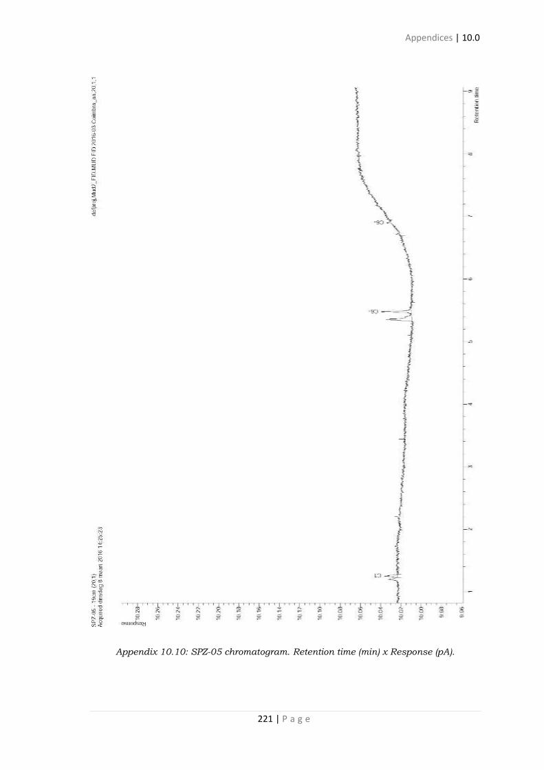
Appendices | 10.0
221 | P a g e
Appendix 10.10: SPZ-05 chromatogram. Retention time (min) x Response (pA).

Appendices | 10.0
222 | P a g e
Appendix 10.11: SPZ-06 chromatogram. Retention time (min) x Response (pA).

Appendices | 10.0
223 | P a g e
Appendix 10.12: SPZ-07 chromatogram. Retention time (min) x Response (pA).

Appendices | 10.0
224 | P a g e
Appendix 10.13: SPZ-08 chromatogram. Retention time (min) x Response (pA).

Appendices | 10.0
225 | P a g e
Appendix 10.14: SPZ-09 chromatogram. Retention time (min) x Response (pA).

Appendices | 10.0
226 | P a g e
Appendix 10.15: SPZ-10 chromatogram. Retention time (min) x Response (pA).

Appendices | 10.0
227 | P a g e
Appendix 10.16: SPZ-11 chromatogram. Retention time (min) x Response (pA).

Appendices | 10.0
228 | P a g e
Appendix 10.17: SPZ-12 chromatogram. Retention time (min) x Response (pA).

Appendices | 10.0
229 | P a g e
Appendix 10.18: SPZ-13 chromatogram. Retention time (min) x Response (pA).

Appendices | 10.0
230 | P a g e
Appendix 10.19: SPZ-14 chromatogram. Retention time (min) x Response (pA).

Appendices | 10.0
231 | P a g e
Appendix 10.20: SPZ-15 chromatogram. Retention time (min) x Response (pA).

Appendices | 10.0
232 | P a g e
Appendix 10.21: SPZ-16 chromatogram. Retention time (min) x Response (pA).

Appendices | 10.0
233 | P a g e
Appendix 10.22: SPZ-17 chromatogram. Retention time (min) x Response (pA).

Appendices | 10.0
234 | P a g e
Appendix 10.23: SPZ-18 chromatogram. Retention time (min) x Response (pA).

Appendices | 10.0
235 | P a g e
Appendix 10.24: SPZ-19 chromatogram. Retention time (min) x Response (pA).

Appendices | 10.0
236 | P a g e
Appendix 10.25: F081 chromatogram. Retention time (min) x Response (pA).

Appendices | 10.0
237 | P a g e
Appendix 10.26: F08 chromatogram. Retention time (min) x Response (pA).

Appendices | 10.0
238 | P a g e
Appendix 10.27: F09 chromatogram. Retention time (min) x Response (pA).

Appendices | 10.0
239 | P a g e
Appendix 10.28: F10 chromatogram. Retention time (min) x Response (pA).

Appendices | 10.0
240 | P a g e
Appendix 10.29: F11 chromatogram. Retention time (min) x Response (pA).

Appendices | 10.0
241 | P a g e
Appendix 10.30: F12 chromatogram. Retention time (min) x Response (pA).

Appendices | 10.0
242 | P a g e
Appendix 10.31: P03 chromatogram. Retention time (min) x Response (pA).

Appendices | 10.0
243 | P a g e
Appendix 10.32: W02 chromatogram. Retention time (min) x Response (pA).

Appendices | 10.0
244 | P a g e
Appendix 10.33: W03 chromatogram. Retention time (min) x Response (pA).

Appendices | 10.0
245 | P a g e
Appendix 10.34: W06 chromatogram. Retention time (min) x Response (pA).

Appendices | 10.0
246 | P a g e
Appendix 10.35: W07 chromatogram. Retention time (min) x Response (pA).

Appendices | 10.0
247 | P a g e
Appendix 10.36: W09 chromatogram. Retention time (min) x Response (pA).

Appendices | 10.0
248 | P a g e
Appendix 10.37: W10 chromatogram. Retention time (min) x Response (pA).

Appendices | 10.0
249 | P a g e
Appendix 10.38: W11 chromatogram. Retention time (min) x Response (pA).

Appendices | 10.0
250 | P a g e
Appendix 10.39: W12 chromatogram. Retention time (min) x Response (pA).
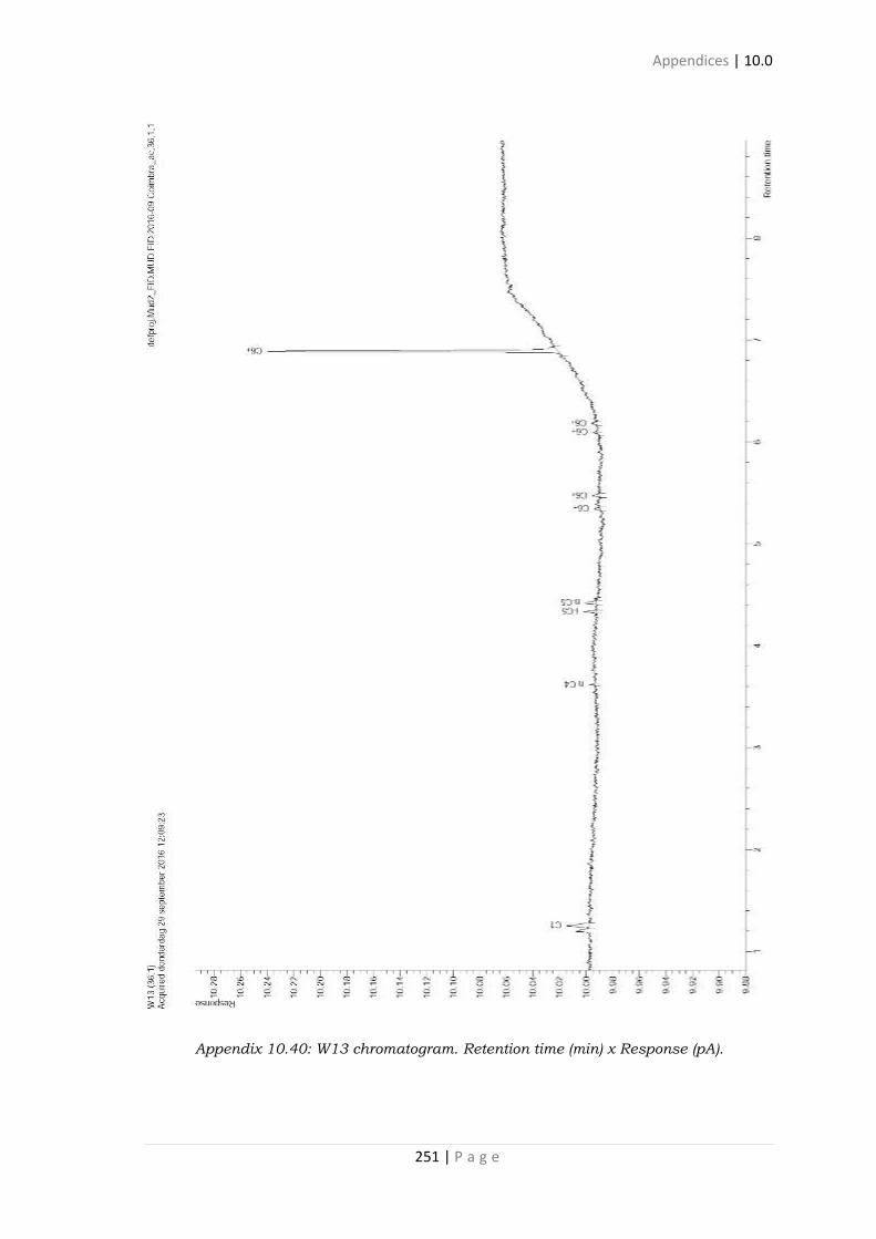
Appendices | 10.0
251 | P a g e
Appendix 10.40: W13 chromatogram. Retention time (min) x Response (pA).

Appendices | 10.0
252 | P a g e
Appendix 10.41: W14 chromatogram. Retention time (min) x Response (pA).

Appendices | 10.0
253 | P a g e
Appendix 10.42: W15 chromatogram. Retention time (min) x Response (pA).

Appendices | 10.0
254 | P a g e
Appendix 10.43: W16 chromatogram. Retention time (min) x Response (pA).

Appendices | 10.0
255 | P a g e
Appendix 10.44: W17 chromatogram. Retention time (min) x Response (pA).

Appendices | 10.0
256 | P a g e
Appendix 10.45: W18 chromatogram. Retention time (min) x Response (pA).

Appendices | 10.0
257 | P a g e
Appendix 10.46: W19 chromatogram. Retention time (min) x Response (pA).

Appendices | 10.0
258 | P a g e
Appendix 10.47: W20 chromatogram. Retention time (min) x Response (pA).

Appendices | 10.0
259 | P a g e
Appendix 10.48: W21 chromatogram. Retention time (min) x Response (pA).

Appendices | 10.0
260 | P a g e
Appendix 10.49: W22 chromatogram. Retention time (min) x Response (pA).

Appendices | 10.0
261 | P a g e
Appendix 10.50: W23 chromatogram. Retention time (min) x Response (pA).

Appendices | 10.0
262 | P a g e
Appendix 10.51: W24 chromatogram. Retention time (min) x Response (pA).

Appendices | 10.0
263 | P a g e
Appendix 10.52: W25 chromatogram. Retention time (min) x Response (pA).

Appendices | 10.0
264 | P a g e
Appendix 10.53: W26 chromatogram. Retention time (min) x Response (pA).

Appendices | 10.0
265 | P a g e
Appendix 10.54: W27 chromatogram. Retention time (min) x Response (pA).

Appendices | 10.0
266 | P a g e
Appendix 10.55: W28 chromatogram. Retention time (min) x Response (pA).

Appendices | 10.0
267 | P a g e
Appendix 10.56: W29 chromatogram. Retention time (min) x Response (pA).

Appendices | 10.0
268 | P a g e
Appendix 10.57: W30 chromatogram. Retention time (min) x Response (pA).

Appendices | 10.0
269 | P a g e
Appendix 10.58: W31 chromatogram. Retention time (min) x Response (pA).
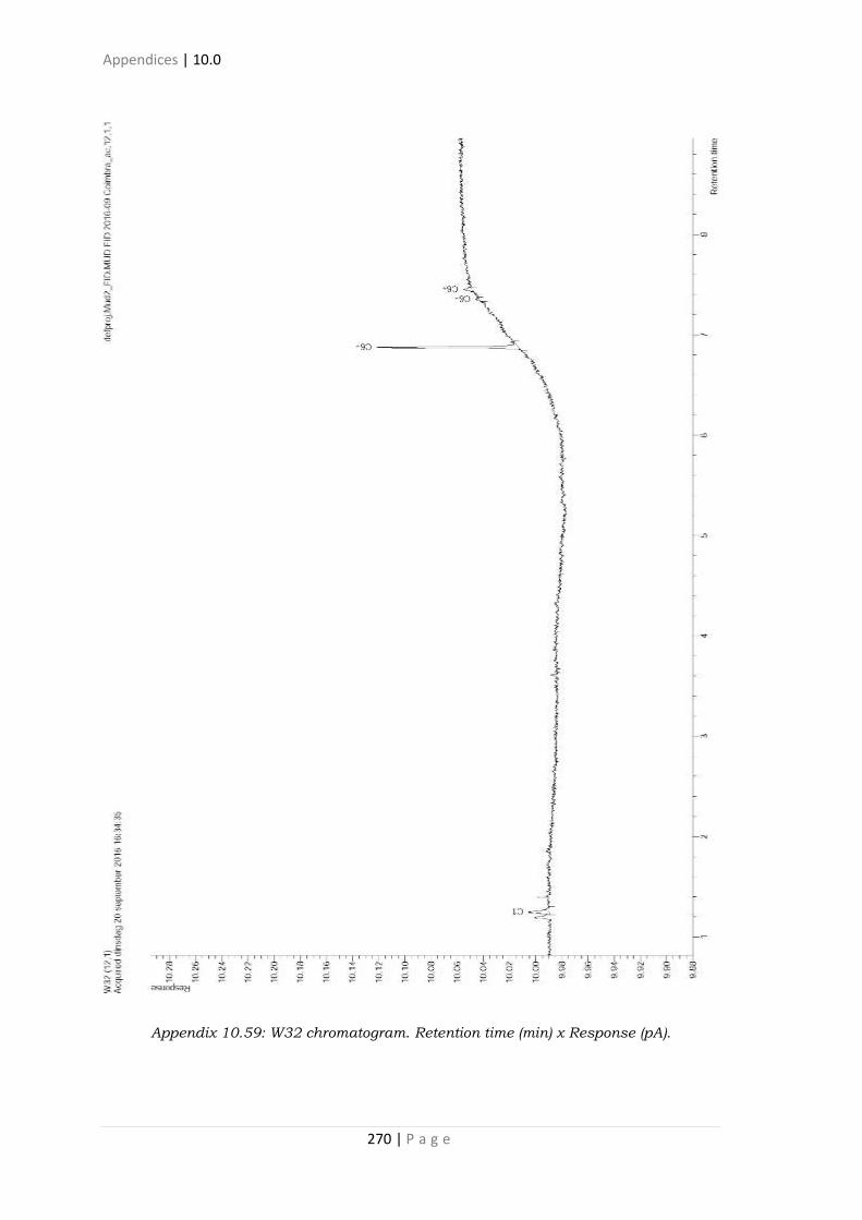
Appendices | 10.0
270 | P a g e
Appendix 10.59: W32 chromatogram. Retention time (min) x Response (pA).

Appendices | 10.0
271 | P a g e
Appendix 10.60: W33 chromatogram. Retention time (min) x Response (pA).

Appendices | 10.0
272 | P a g e
Appendix 10.61: W331 chromatogram. Retention time (min) x Response (pA).

Appendices | 10.0
273 | P a g e
Appendix 10.62: W34 chromatogram. Retention time (min) x Response (pA).


Appendices | 10.0
275 | P a g e
Appendix 10.63: Sample locations. and BAFG geological framework.


Appendices | 10.0
277 | P a g e
Appendix 10.64: Water and soil sample locations.


Appendices | 10.0
279 | P a g e
Appendix 12.65: Rock-eval samples locations.