Unconventional reservoir characterization using ... · PDF fileUnconventional reservoir characterization using conventional tools . Ritesh K. Sharma* and Satinder Chopra . Arcis Seismic

Unconventional reservoir characterization using conventional tools

Ritesh K. Sharma* and Satinder Chopra

Arcis Seismic Solutions, TGS, Calgary, Canada

Summary

Shale resources characterization has gained attention in the last

decade or so, after the Mississippian Barnett shale was

successfully developed with the application of hydraulic fracing

and horizontal drilling. For characterization of shale gas

formations different workflows using 3D surface seismic data have been introduced. We propose an integrated workflow for

the characterization of the Montney shale formation, one of the

largest and economically viable resource plays in North

America. We also compare results to those that were obtained

by an existing workflow described elsewhere.

Introduction

Shale-gas plays differ from conventional gas plays in that the

shale formations are both the source rocks and the reservoir

rocks. There is no migration of gas as the very low permeability

of the rock causes the rock to trap the gas and it forms its own

seal. The gas can be held in natural fractures or pore space, or can be absorbed onto the organic material (Curtis, 2002). Apart

from the permeability, total organic content (TOC) and thermal

maturity are the key properties of gas potential shale. Generally,

it can be stated that the higher the TOC, the better the potential

for hydrocarbon generation. In addition to these characteristics, thickness, gas-in-place, mineralogy, brittleness, pore space and

the depth of the shale gas formation are other characteristics that

need to be considered for a shale gas reservoir to become a

successful shale gas play. The organic content in these shales,

which are measured by their TOC ratings, influence the compressional and shear velocities as well as the density and

anisotropy in these formations. Consequently, it should be

possible to detect changes in TOC from the surface seismic

response.

The method

Passey et al. (1990) proposed a technique for measuring TOC in

shale gas formations. Basically, this technique is based on the

porosity-resistivity overlay to locate hydrocarbon bearing shale

pockets. Usually, the sonic log is used as the porosity indicator.

In this technique, the transit time curve and the resistivity curves

are scaled in such a way that the sonic curve lies on top of the

resistivity curve over a large depth range, except for organic-rich

intervals where they would show crossover between themselves.

TOC changes in shale formations influence VP, VS, density and

anisotropy and thus should be detected on the seismic response.

To detect it, different workflows have been discussed by Chopra

et al. (2012).

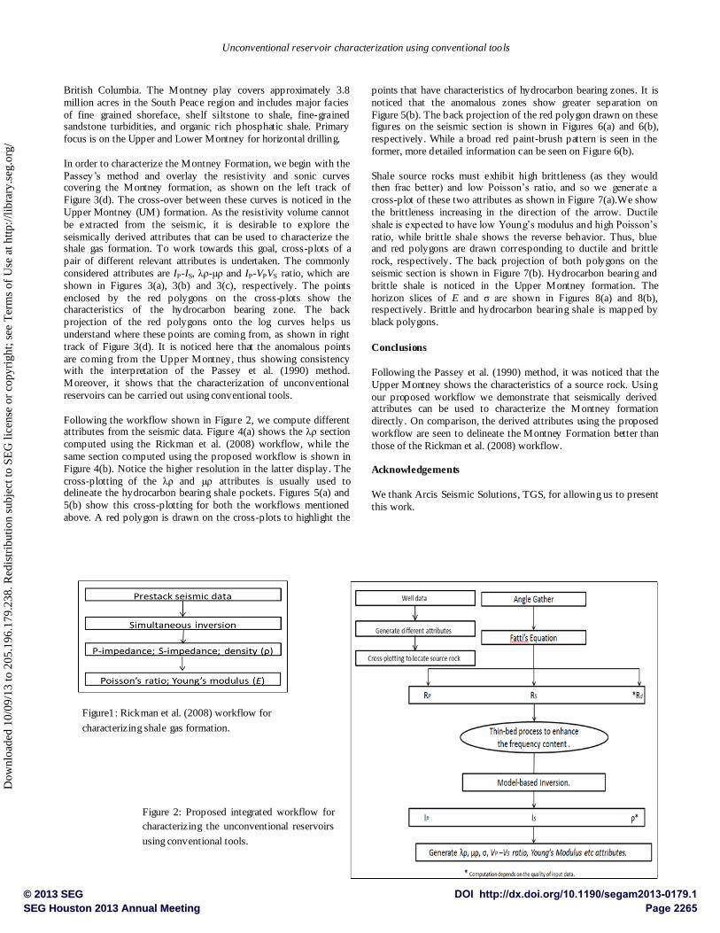
Rickman et al. (2008) showed that brittleness of a rock formation

can be estimated from the computed Poisson’s ratio and Young’s

modulus well log curves. This suggests a workflow for estimating

brittleness from 3D seismic data, by way of simultaneous pre-stack

inversion that yields IP, IS, VP/VS, Poisson’s ratio, and in some

cases meaningful estimates of density. Zones with high Young’s

modulus and low Poisson’s ratio are those that would be brittle as

well as have better reservoir quality (higher TOC, higher porosity).

Such a workflow works well for good quality data and is shown in

Figure 1.

We propose an integrated work flow in which well data as well as

seismic data are used to characterize the hydrocarbon bearing shale

as shown in Figure 2. We begin with the generation of different

attributes from the well-log curves. Then, using the cross-plots of

these attributes we try and identify the hydrocarbon bearing shale

zones. Once this analysis is done at the well locations, seismic data

analysis is picked up for computing appropriate attributes.

Seismically, pre-stack data is essentially the starting point. After

generating angle gathers from the conditioned offset gathers,

Fatti’s equation (Fatti et al. 1994) can be used to compute P-

reflectivity, S-reflectivity, and density which depends on the

quality of input data as well as the presence of long offsets. Due to

the band-limited nature of acquired seismic data, any attribute

extracted from it will also be band-limited, and so will have a

limited resolution. While shale formations may be thick, some high

TOC shale units may be thin. So, it is desirable to enhance the

resolution of the seismic data. An appropriate way of doing it is the

thin-bed reflectivity inversion (Chopra et al. 2006; Puryear and

Castagna, 2008). Following this process, the wavelet effect is

removed from the data and the output of the inversion process can

be viewed as spectrally broadened seismic data, retrieved in the

form of broadband reflectivity data that can be filtered back to any

bandwidth. This usually represents useful information for

interpretation purposes. Thin-bed reflectivity serves to provide the

reflection character that can be studied, by convolving the

reflectivity with a wavelet of a known frequency band-pass. This

not only provides an opportunity to study reflection character

associated with features of interest, but also serves to confirm its

close match with the original data. Further, the output of thin-bed

inversion is considered as input for the model based inversion to

compute P-impedance, S-impedance and density. Once

impedances are obtained, we can compute other relevant attributes,

such as the λρ, μρ and VP/VS. These are used to measure the pore

space properties and get information about the rock skeleton.

Young’s modulus can be treated as brittleness indicators and

Poisson’s ratio as TOC indicator.

Examples

The Montney play is one of the active natural gas plays in North

America. It is a thick, regionally charged formation of unconventional tight gas/shale distributed in an area extending

from north central Alberta to the northwest of Fort St. John in

DOI http://dx.doi.org/10.1190/segam2013-0179.1© 2013 SEGSEG Houston 2013 Annual Meeting Page 2264

Dow

nloa

ded

10/0

9/13

to 2

05.1

96.1

79.2

38. R

edis

trib

utio

n su

bjec

t to

SEG

lice

nse

or c

opyr

ight

; see

Ter

ms

of U

se a

t http

://lib

rary

.seg

.org

/


British Columbia. The Montney play covers approximately 3.8

million acres in the South Peace region and includes major facies

of fine grained shoreface, shelf siltstone to shale, fine-grained sandstone turbidities, and organic rich phosphatic shale. Primary

focus is on the Upper and Lower Montney for horizontal drilling.

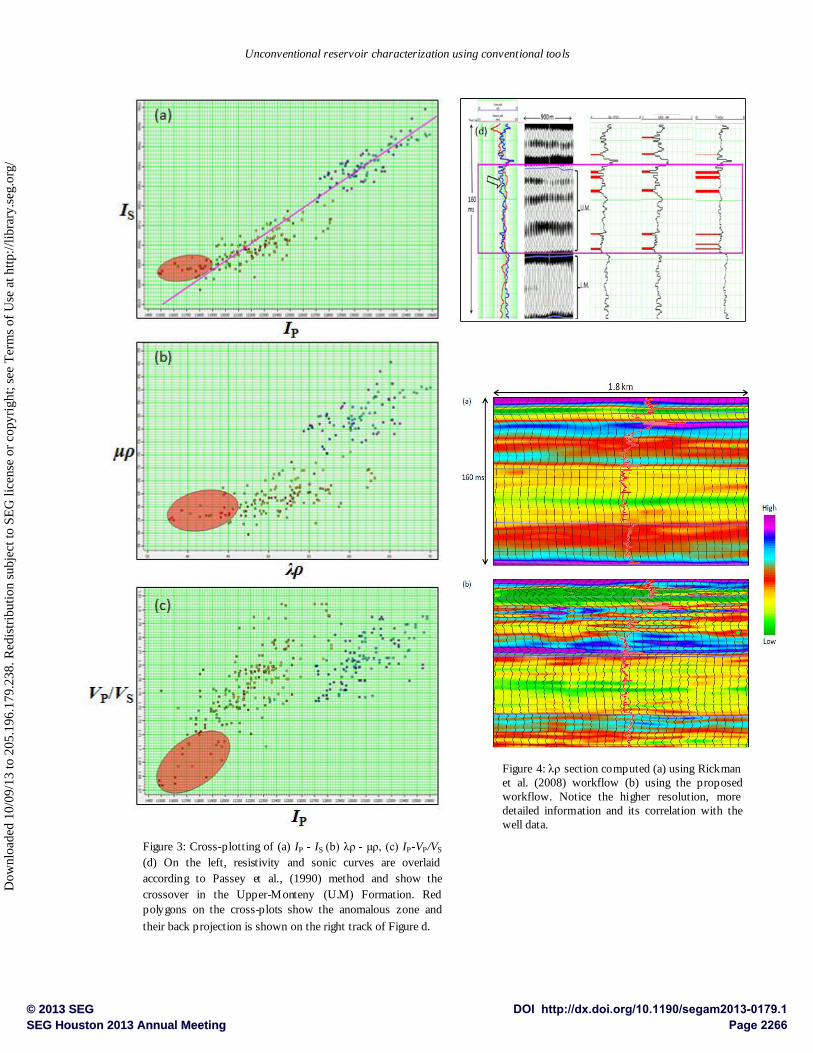
In order to characterize the Montney Formation, we begin with the

Passey’s method and overlay the resistivity and sonic curves covering the Montney formation, as shown on the left track of

Figure 3(d). The cross-over between these curves is noticed in the

Upper Montney (UM) formation. As the resistivity volume cannot

be extracted from the seismic, it is desirable to explore the

seismically derived attributes that can be used to characterize the shale gas formation. To work towards this goal, cross-plots of a

pair of different relevant attributes is undertaken. The commonly

considered attributes are IP-IS, λρ-μρ and IP-VPVS ratio, which are

shown in Figures 3(a), 3(b) and 3(c), respectively. The points

enclosed by the red polygons on the cross-plots show the characteristics of the hydrocarbon bearing zone. The back

projection of the red polygons onto the log curves helps us

understand where these points are coming from, as shown in right

track of Figure 3(d). It is noticed here that the anomalous points

are coming from the Upper Montney, thus showing consistency with the interpretation of the Passey et al. (1990) method.

Moreover, it shows that the characterization of unconventional

reservoirs can be carried out using conventional tools.

Following the workflow shown in Figure 2, we compute different attributes from the seismic data. Figure 4(a) shows the λρ section

computed using the Rickman et al. (2008) workflow, while the

same section computed using the proposed workflow is shown in

Figure 4(b). Notice the higher resolution in the latter display. The

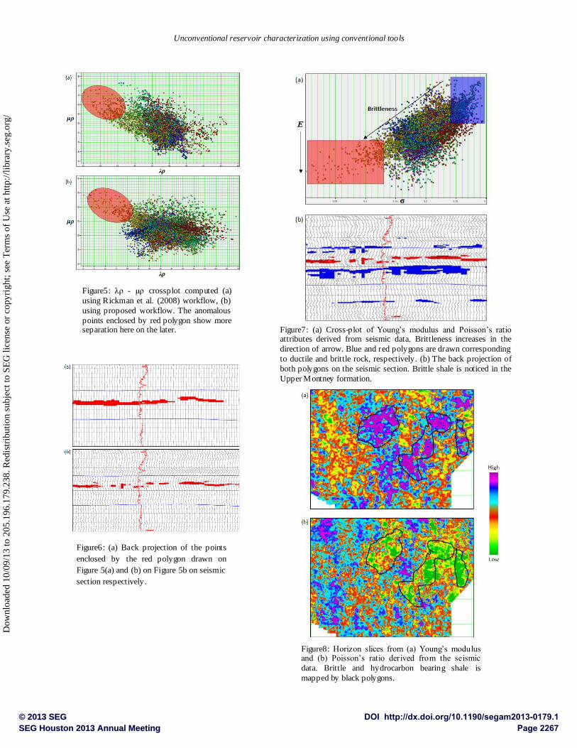
cross-plotting of the λρ and μρ attributes is usually used to delineate the hydrocarbon bearing shale pockets. Figures 5(a) and

5(b) show this cross-plotting for both the workflows mentioned

above. A red polygon is drawn on the cross-plots to highlight the

points that have characteristics of hydrocarbon bearing zones. It is

noticed that the anomalous zones show greater separation on

Figure 5(b). The back projection of the red polygon drawn on these figures on the seismic section is shown in Figures 6(a) and 6(b),

respectively. While a broad red paint-brush pattern is seen in the

former, more detailed information can be seen on Figure 6(b).

Shale source rocks must exhibit high brittleness (as they would then frac better) and low Poisson’s ratio, and so we generate a

cross-plot of these two attributes as shown in Figure 7(a).We show

the brittleness increasing in the direction of the arrow. Ductile

shale is expected to have low Young’s modulus and high Poisson’s

ratio, while brittle shale shows the reverse behavior. Thus, blue and red polygons are drawn corresponding to ductile and brittle

rock, respectively. The back projection of both polygons on the

seismic section is shown in Figure 7(b). Hydrocarbon bearing and

brittle shale is noticed in the Upper Montney formation. The

horizon slices of E and σ are shown in Figures 8(a) and 8(b), respectively. Brittle and hydrocarbon bearing shale is mapped by

black polygons.

Conclusions

Following the Passey et al. (1990) method, it was noticed that the

Upper Montney shows the characteristics of a source rock. Using

our proposed workflow we demonstrate that seismically derived attributes can be used to characterize the Montney formation

directly. On comparison, the derived attributes using the proposed

workflow are seen to delineate the Montney Formation better than

those of the Rickman et al. (2008) workflow.

Acknowledgements

We thank Arcis Seismic Solutions, TGS, for allowing us to present

this work.

Figure1: Rickman et al. (2008) workflow for

characterizing shale gas formation.

Figure 2: Proposed integrated workflow for

characterizing the unconventional reservoirs

using conventional tools.


Dow

nloa

ded

10/0

9/13

to 2

05.1

96.1

79.2

38. R

edis

trib

utio

n su

bjec

t to

SEG

lice

nse

or c

opyr

ight

; see

Ter

ms

of U

se a

t http

://lib

rary

.seg

.org

/


Figure 3: Cross-plotting of (a) IP - IS (b) λρ - μρ, (c) IP-VP/VS

(d) On the left, resistivity and sonic curves are overlaid

according to Passey et al., (1990) method and show the

crossover in the Upper-Monteny (U.M) Formation. Red

polygons on the cross-plots show the anomalous zone and

their back projection is shown on the right track of Figure d.

Figure 4: λρ section computed (a) using Rickman

et al. (2008) workflow (b) using the proposed

workflow. Notice the higher resolution, more

detailed information and its correlation with the

well data.


Dow

nloa

ded

10/0

9/13

to 2

05.1

96.1

79.2

38. R

edis

trib

utio

n su

bjec

t to

SEG

lice

nse

or c

opyr

ight

; see

Ter

ms

of U

se a

t http

://lib

rary

.seg

.org

/


Figure5: λρ - μρ crossplot computed (a)

using Rickman et al. (2008) workflow, (b)

using proposed workflow. The anomalous

points enclosed by red polygon show more separation here on the later.

Figure6: (a) Back projection of the points

enclosed by the red polygon drawn on

Figure 5(a) and (b) on Figure 5b on seismic

section respectively.

Figure7: (a) Cross-plot of Young’s modulus and Poisson’s ratio attributes derived from seismic data. Brittleness increases in the

direction of arrow. Blue and red polygons are drawn corresponding

to ductile and brittle rock, respectively. (b) The back projection of

both polygons on the seismic section. Brittle shale is noticed in the

Upper Montney formation.

Figure8: Horizon slices from (a) Young’s modulus and (b) Poisson’s ratio derived from the seismic

data. Brittle and hydrocarbon bearing shale is

mapped by black polygons.


Dow

nloa

ded

10/0

9/13

to 2

05.1

96.1

79.2

38. R

edis

trib

utio

n su

bjec

t to

SEG

lice

nse

or c

opyr

ight

; see

Ter

ms

of U

se a

t http

://lib

rary

.seg

.org

/

http://dx.doi.org/10.1190/segam2013-0179.1 EDITED REFERENCES Note: This reference list is a copy-edited version of the reference list submitted by the author. Reference lists for the 2013 SEG Technical Program Expanded Abstracts have been copy edited so that references provided with the online metadata for each paper will achieve a high degree of linking to cited sources that appear on the Web. REFERENCES

Chopra, S., J. P. Castagna, and O. Portniaguine, 2006, Seismic resolution and thin-bed reflectivity inversion: CSEG Recorder, 31, 19–25.

Chopra, S., R. K. Sharma, J. Keay, and K. J. Marfurt, 2012, Shale gas reservoir characterization work flow: 82nd Annual International Meeting, SEG, Expanded Abstracts, http://dx.doi.org/10.1190/segam2012-1344.1.

Curtis , J. B., 2002, Fractured shale gas systems: AAPG Bulletin, 86, 1921–1938.

Fatti, J., G. Smith, P. Vail, P. Strauss, and P. Levitt, 1994, Detection of gas in sandstone reservoirs using AVO analysis: A 3D seismic case history using the Geostack technique : Geophysics, 59, 1362–1376, http://dx.doi.org/10.1190/1.1443695.

Passey, Q. R., S. Creaney, J. B. Kulla, F. J. Moretti, and J. D. Stroud, 1990, A practical model for organic richness from porosity and resistivity logs : AAPG Bulletin , 74, 1777–1794.

Puryear, C. I., and J. P. Castagna, 2008, Layer-thickness determination and stratigraphic interpretation using spectral inversion: Theory and application: Geophysics, 73, no. 2, R37–R48, http://dx.doi.org/10.1190/1.2838274.

Rickman, R., M. Mullen, E. Petre, B. Grieser, and D. Kundert, 2008, A practical use of shale petrophysics for stimulation design optimization: All shale plays are not clones of the Barnett Shale: Annual Technical Conference and Exhibition, Society of Petroleum Engineers, SPE 11528.


Dow

nloa

ded

10/0

9/13

to 2

05.1

96.1

79.2

38. R

edis

trib

utio

n su

bjec

t to

SEG

lice

nse

or c

opyr

ight

; see

Ter

ms

of U

se a

t http

://lib

rary

.seg

.org

/

Documents

Unconventional reservoir characterization using ... · PDF fileUnconventional reservoir characterization using conventional tools . Ritesh K. Sharma* and Satinder Chopra . Arcis Seismic