Under review as a conference paper at ICLR 2017 · Under review as a conference paper at ICLR 2017 RL 2: FAST R EINFORCEMENT L EARNING VIA S LOW R EINFORCEMENT L EARNING Yan Duan

Under review as a conference paper at ICLR 2017

RL2: FAST REINFORCEMENT LEARNING VIA SLOWREINFORCEMENT LEARNING

Yan Duan†‡, John Schulman†‡, Xi Chen†‡, Peter L. Bartlett†, Ilya Sutskever‡, Pieter Abbeel†‡† UC Berkeley, Department of Electrical Engineering and Computer Science‡ OpenAI{rocky,joschu,peter}@openai.com, [email protected], {ilyasu,pieter}@openai.com

ABSTRACT

Deep reinforcement learning (deep RL) has been successful in learning sophis-ticated behaviors automatically; however, the learning process requires a hugenumber of trials. In contrast, animals can learn new tasks in just a few trials, bene-fiting from their prior knowledge about the world. This paper seeks to bridge thisgap. Rather than designing a “fast” reinforcement learning algorithm, we proposeto represent it as a recurrent neural network (RNN) and learn it from data. Inour proposed method, RL2, the algorithm is encoded in the weights of the RNN,which are learned slowly through a general-purpose (“slow”) RL algorithm. TheRNN receives all information a typical RL algorithm would receive, including ob-servations, actions, rewards, and termination flags; and it retains its state acrossepisodes in a given Markov Decision Process (MDP). The activations of the RNNstore the state of the “fast” RL algorithm on the current (previously unseen) MDP.We evaluate RL2 experimentally on both small-scale and large-scale problems.On the small-scale side, we train it to solve randomly generated multi-armed ban-dit problems and finite MDPs. After RL2 is trained, its performance on new MDPsis close to human-designed algorithms with optimality guarantees. On the large-scale side, we test RL2 on a vision-based navigation task and show that it scalesup to high-dimensional problems.

1 INTRODUCTION

In recent years, deep reinforcement learning has achieved many impressive results, including playingAtari games from raw pixels (Guo et al., 2014; Mnih et al., 2015; Schulman et al., 2015), andacquiring advanced manipulation and locomotion skills (Levine et al., 2016; Lillicrap et al., 2015;Watter et al., 2015; Heess et al., 2015; Schulman et al., 2015; 2016). However, many of the successescome at the expense of high sample complexity. For example, the state-of-the-art Atari resultsrequire tens of thousands of episodes of experience (Mnih et al., 2015) per game. To master a game,one would need to spend nearly 40 days playing it with no rest. In contrast, humans and animals arecapable of learning a new task in a very small number of trials. Continuing the previous example,the human player in Mnih et al. (2015) only needed 2 hours of experience before mastering a game.We argue that the reason for this sharp contrast is largely due to the lack of a good prior, whichresults in these deep RL agents needing to rebuild their knowledge about the world from scratch.

Although Bayesian reinforcement learning provides a solid framework for incorporating priorknowledge into the learning process (Strens, 2000; Ghavamzadeh et al., 2015; Kolter & Ng, 2009),exact computation of the Bayesian update is intractable in all but the simplest cases. Thus, practi-cal reinforcement learning algorithms often incorporate a mixture of Bayesian and domain-specificideas to bring down sample complexity and computational burden. Notable examples include guidedpolicy search with unknown dynamics (Levine & Abbeel, 2014) and PILCO (Deisenroth & Ras-mussen, 2011). These methods can learn a task using a few minutes to a few hours of real experience,compared to days or even weeks required by previous methods (Schulman et al., 2015; 2016; Lilli-crap et al., 2015). However, these methods tend to make assumptions about the environment (e.g.,instrumentation for access to the state at learning time), or become computationally intractable inhigh-dimensional settings (Wahlstrom et al., 2015).

1

arX

iv:1

611.

0277

9v2

[cs

.AI]

10

Nov

201

6


Rather than hand-designing domain-specific reinforcement learning algorithms, we take a differentapproach in this paper: we view the learning process of the agent itself as an objective, which canbe optimized using standard reinforcement learning algorithms. The objective is averaged acrossall possible MDPs according to a specific distribution, which reflects the prior that we would liketo distill into the agent. We structure the agent as a recurrent neural network, which receives pastrewards, actions, and termination flags as inputs in addition to the normally received observations.Furthermore, its internal state is preserved across episodes, so that it has the capacity to performlearning in its own hidden activations. The learned agent thus also acts as the learning algorithm,and can adapt to the task at hand when deployed.

We evaluate this approach on two sets of classical problems, multi-armed bandits and tabular MDPs.These problems have been extensively studied, and there exist algorithms that achieve asymptoti-cally optimal performance. We demonstrate that our method, named RL2, can achieve performancecomparable with these theoretically justified algorithms. Next, we evaluate RL2 on a vision-basednavigation task implemented using the ViZDoom environment (Kempka et al., 2016), showing thatRL2 can also scale to high-dimensional problems.

2 METHOD

2.1 PRELIMINARIES

We define a discrete-time finite-horizon discounted Markov decision process (MDP) by a tupleM =(S,A,P, r, ρ0, γ, T ), in which S is a state set, A an action set, P : S × A × S → R+ a transitionprobability distribution, r : S ×A → [−Rmax, Rmax] a bounded reward function, ρ0 : S → R+ aninitial state distribution, γ ∈ [0, 1] a discount factor, and T the horizon. In policy search methods,we typically optimize a stochastic policy πθ : S × A → R+ parametrized by θ. The objective isto maximize its expected discounted return, η(πθ) = Eτ [

∑Tt=0 γ

tr(st, at)], where τ = (s0, a0, . . .)denotes the whole trajectory, s0 ∼ ρ0(s0), at ∼ πθ(at|st), and st+1 ∼ P(st+1|st, at).

2.2 FORMULATION

We now describe our formulation, which casts learning an RL algorithm as a reinforcement learningproblem, and hence the name RL2. We assume knowledge of a set of MDPs, denoted byM, and adistribution over them: ρM :M→ R+. We only need to sample from this distribution. We use nto denote the total number of episodes allowed to spend with a specific MDP. We define a trial to besuch a series of episodes of interaction with a fixed MDP.

Episode 1 Episode 2

s0 s1 s2

h0 h1

a0

r0,d0

h2 h3

s3

a1

r1,d1

a2

r2,d2

s0 s1 s2

h4 h5

a0

r0,d0

h6

a1

r1,d1

Agent

MDP 1Episode 1

s0 s1 …

h0 h1

a0

r0,d0

…

a1

Agent

MDP 2…

…

…

Trial 1 Trial 2

Figure 1: Procedure of agent-environment interaction

This process of interaction between an agent and the environment is illustrated in Figure 1. Here,each trial happens to consist of two episodes, hence n = 2. For each trial, a separate MDP isdrawn from ρM, and for each episode, a fresh s0 is drawn from the initial state distribution specificto the corresponding MDP. Upon receiving an action at produced by the agent, the environmentcomputes reward rt, steps forward, and computes the next state st+1. If the episode has terminated,it sets termination flag dt to 1, which otherwise defaults to 0. Together, the next state st+1, action

2


at, reward rt, and termination flag dt, are concatenated to form the input to the policy1, which,conditioned on the hidden state ht+1, generates the next hidden state ht+2 and action at+1. At theend of an episode, the hidden state of the policy is preserved to the next episode, but not preservedbetween trials.

The objective under this formulation is to maximize the expected total discounted reward accumu-lated during a single trial rather than a single episode. Maximizing this objective is equivalent tominimizing the cumulative pseudo-regret (Bubeck & Cesa-Bianchi, 2012). Since the underlyingMDP changes across trials, as long as different strategies are required for different MDPs, the agentmust act differently according to its belief over which MDP it is currently in. Hence, the agent isforced to integrate all the information it has received, including past actions, rewards, and termi-nation flags, and adapt its strategy continually. Hence, we have set up an end-to-end optimizationprocess, where the agent is encouraged to learn a “fast” reinforcement learning algorithm.

For clarity of exposition, we have defined the “inner” problem (of which the agent sees n each trials)to be an MDP rather than a POMDP. However, the method can also be applied in the partially-observed setting without any conceptual changes. In the partially observed setting, the agent isfaced with a sequence of POMDPs, and it receives an observation ot instead of state st at time t.The visual navigation experiment in Section 3.3, is actually an instance of the this POMDP setting.

2.3 POLICY REPRESENTATION

We represent the policy as a general recurrent neural network. Each timestep, it receives the tuple(s, a, r, d) as input, which is embedded using a function φ(s, a, r, d) and provided as input to anRNN. To alleviate the difficulty of training RNNs due to vanishing and exploding gradients (Bengioet al., 1994), we use Gated Recurrent Units (GRUs) (Cho et al., 2014) which have been demonstratedto have good empirical performance (Chung et al., 2014; Jozefowicz et al., 2015). The output of theGRU is fed to a fully connected layer followed by a softmax function, which forms the distributionover actions.

We have also experimented with alternative architectures which explicitly reset part of the hiddenstate each episode of the sampled MDP, but we did not find any improvement over the simple archi-tecture described above.

2.4 POLICY OPTIMIZATION

After formulating the task as a reinforcement learning problem, we can readily use standard off-the-shelf RL algorithms to optimize the policy. We use a first-order implementation of Trust RegionPolicy Optimization (TRPO) (Schulman et al., 2015), because of its excellent empirical perfor-mance, and because it does not require excessive hyperparameter tuning. For more details, we referthe reader to the original paper. To reduce variance in the stochastic gradient estimation, we use abaseline which is also represented as an RNN using GRUs as building blocks. We optionally applyGeneralized Advantage Estimation (GAE) (Schulman et al., 2016) to further reduce the variance.

3 EVALUATION

We designed experiments to answer the following questions:

• Can RL2 learn algorithms that achieve good performance on MDP classes with specialstructure, relative to existing algorithms tailored to this structure that have been proposedin the literature?

• Can RL2 scale to high-dimensional tasks?

For the first question, we evaluate RL2 on two sets of tasks, multi-armed bandits (MAB) and tabularMDPs. These problems have been studied extensively in the reinforcement learning literature, andthis body of work includes algorithms with guarantees of asymptotic optimality. We demonstratethat our approach achieves comparable performance to these theoretically justified algorithms.

1To make sure that the inputs have a consistent dimension, we use placeholder values for the initial input tothe policy.

3


For the second question, we evaluate RL2 on a vision-based navigation task. Our experiments showthat the learned policy makes effective use of the learned visual information and also short-terminformation acquired from previous episodes.

3.1 MULTI-ARMED BANDITS

Multi-armed bandit problems are a subset of MDPs where the agent’s environment is stateless.Specifically, there are k arms (actions), and at every time step, the agent pulls one of the arms, sayi, and receives a reward drawn from an unknown distribution: our experiments take each arm tobe a Bernoulli distribution with parameter pi. The goal is to maximize the total reward obtainedover a fixed number of time steps. The key challenge is balancing exploration and exploitation—“exploring” each arm enough times to estimate its distribution (pi), but eventually switching over to“exploitation” of the best arm. Despite the simplicity of multi-arm bandit problems, their study hasled to a rich theory and a collection of algorithms with optimality guarantees.

Using RL2, we can train an RNN policy to solve bandit problems by training it on a given distributionρM. If the learning is successful, the resulting policy should be able to perform competitively withthe theoretically optimal algorithms. We randomly generated bandit problems by sampling eachparameter pi from the uniform distribution on [0, 1]. After training the RNN policy with RL2, wecompared it against the following strategies:

• Random: this is a baseline strategy, where the agent pulls a random arm each time.

• Gittins index (Gittins, 1979): this method gives the Bayes optimal solution in the dis-counted infinite-horizon case, by computing an index separately for each arm, and takingthe arm with the largest index. While this work shows it is sufficient to independently com-pute an index for each arm (hence avoiding combinatorial explosion with the number ofarms), it doesn’t show how to tractably compute these individual indices exactly. We fol-low the practical approximations described in Gittins et al. (2011), Chakravorty & Mahajan(2013), and Whittle (1982), and choose the best-performing approximation for each setup.

• UCB1 (Auer, 2002): this method estimates an upper-confidence bound, and pulls the arm

with the largest value of ucbi(t) = µi(t−1)+c√

2 log tTi(t−1) , where µi(t−1) is the estimated

mean parameter for the ith arm, Ti(t−1) is the number of times the ith arm has been pulled,and c is a tunable hyperparameter (Audibert & Munos, 2011). We initialize the statisticswith exactly one success and one failure, which corresponds to a Beta(1, 1) prior.

• Thompson sampling (TS) (Thompson, 1933): this is a simple method which, at each timestep, samples a list of arm means from the posterior distribution, and choose the best armaccording to this sample. It has been demonstrated to compare favorably to UCB1 empir-ically (Chapelle & Li, 2011). We also experiment with an optimistic variant (OTS) (Mayet al., 2012), which samples N times from the posterior, and takes the one with the highestprobability.

• ε-Greedy: in this strategy, the agent chooses the arm with the best empirical mean withprobability 1 − ε, and chooses a random arm with probability ε. We use the same initial-ization as UCB1.

• Greedy: this is a special case of ε-Greedy with ε = 0.

The Bayesian methods, Gittins index and Thompson sampling, take advantage of the distributionρM; and we provide these methods with the true distribution. For each method with hyperparame-ters, we maximize the score with a separate grid search for each of the experimental settings. Thehyperparameters used for TRPO are shown in the appendix.

The results are summarized in Table 1. Learning curves for various settings are shown in Figure 2.We observe that our approach achieves performance that is almost as good as the the reference meth-ods, which were (human) designed specifically to perform well on multi-armed bandit problems. Itis worth noting that the published algorithms are mostly designed to minimize asymptotic regret(rather than finite horizon regret), hence there tends to be a little bit of room to outperform them inthe finite horizon settings.

4


Table 1: MAB Results. Each grid cell records the total reward averaged over 1000 different instancesof the bandit problem. We consider k ∈ {5, 10, 50} bandits and n ∈ {10, 100, 500} episodes ofinteraction. We highlight the best-performing algorithms in each setup according to the computedmean, and we also highlight the other algorithms in that row whose performance is not significantlydifferent from the best one (determined by a one-sided t-test with p = 0.05).

Setup Random Gittins TS OTS UCB1 ε-Greedy Greedy RL2

n = 10, k = 5 5.0 6.6 5.7 6.5 6.7 6.6 6.6 6.7n = 10, k = 10 5.0 6.6 5.5 6.2 6.7 6.6 6.6 6.7n = 10, k = 50 5.1 6.5 5.2 5.5 6.6 6.5 6.5 6.8n = 100, k = 5 49.9 78.3 74.7 77.9 78.0 75.4 74.8 78.7n = 100, k = 10 49.9 82.8 76.7 81.4 82.4 77.4 77.1 83.5n = 100, k = 50 49.8 85.2 64.5 67.7 84.3 78.3 78.0 84.9n = 500, k = 5 249.8 405.8 402.0 406.7 405.8 388.2 380.6 401.6n = 500, k = 10 249.0 437.8 429.5 438.9 437.1 408.0 395.0 432.5n = 500, k = 50 249.6 463.7 427.2 437.6 457.6 413.6 402.8 438.9

0 300Iteration

0

1

Nor

mal

ized

tota

l rew

ard

k = 5k = 10k = 50Gittins

(a) n = 10

0 600Iteration

0

1

Nor

mal

ized

tota

l rew

ard


(b) n = 100

0 600Iteration

0

1

Nor

mal

ized

tota

l rew

ard


(c) n = 500

Figure 2: RL2 learning curves for multi-armed bandits. Performance is normalized such that Gittinsindex scores 1, and random policy scores 0.

We observe that there is a noticeable gap between Gittins index and RL2 in the most challengingscenario, with 50 arms and 500 episodes. This raises the question whether better architecturesor better (slow) RL algorithms should be explored. To determine the bottleneck, we trained thesame policy architecture using supervised learning, using the trajectories generated by the Gittinsindex approach as training data. We found that the learned policy, when executed in test domains,achieved the same level of performance as the Gittins index approach, suggesting that there is roomfor improvement by using better RL algorithms.

3.2 TABULAR MDPS

The bandit problem provides a natural and simple setting to investigate whether the policy learnsto trade off between exploration and exploitation. However, the problem itself involves no sequen-tial decision making, and does not fully characterize the challenges in solving MDPs. Hence, weperform further experiments using randomly generated tabular MDPs, where there is a finite num-ber of possible states and actions—small enough that the transition probability distribution can beexplicitly given as a table. We compare our approach with the following methods:

• Random: the agent chooses an action uniformly at random for each time step;• PSRL (Strens, 2000; Osband et al., 2013): this is a direct generalization of Thompson sam-

pling to MDPs, where at the beginning of each episode, we sample an MDP from the pos-terior distribution, and take actions according to the optimal policy for the entire episode.Similarly, we include an optimistic variant (OPSRL), which has also been explored in Os-band & Van Roy (2016).• BEB (Kolter & Ng, 2009): this is a model-based optimistic algorithm that adds an explo-

ration bonus to (thus far) infrequently visited states and actions.

5


• UCRL2 (Jaksch et al., 2010): this algorithm computes, at each iteration, the optimal pol-icy against an optimistic MDP under the current belief, using an extended value iterationprocedure.

• ε-Greedy: this algorithm takes actions optimal against the MAP estimate according to thecurrent posterior, which is updated once per episode.

• Greedy: a special case of ε-Greedy with ε = 0.

Table 2: Random MDP Results

Setup Random PSRL OPSRL UCRL2 BEB ε-Greedy Greedy RL2

n = 10 100.1 138.1 144.1 146.6 150.2 132.8 134.8 156.2n = 25 250.2 408.8 425.2 424.1 427.8 377.3 368.8 445.7n = 50 499.7 904.4 930.7 918.9 917.8 823.3 769.3 936.1n = 75 749.9 1417.1 1449.2 1427.6 1422.6 1293.9 1172.9 1428.8n = 100 999.4 1939.5 1973.9 1942.1 1935.1 1778.2 1578.5 1913.7

The distribution over MDPs is constructed with |S| = 10, |A| = 5. The rewards follow a Gaus-sian distribution with unit variance, and the mean parameters are sampled independently fromNormal(1, 1). The transitions are sampled from a flat Dirichlet distribution. This constructionmatches the commonly used prior in Bayesian RL methods. We set the horizon for each episode tobe T = 10, and an episode always starts on the first state.

0 1000 5000Iteration

0

1

Nor

mal

ized

tota

l rew

ard

n = 10n = 25n = 50n = 75n = 100OPSRL

Figure 3: RL2 learning curves for tabular MDPs. Performance is normalized such that OPSRLscores 1, and random policy scores 0.

The results are summarized in Table 2, and the learning curves are shown in Figure 3. We followthe same evaluation procedure as in the bandit case. We experiment with n ∈ {10, 25, 50, 75, 100}.For fewer episodes, our approach surprisingly outperforms existing methods by a large margin. Theadvantage is reversed as n increases, suggesting that the reinforcement learning problem in the outerloop becomes more challenging to solve. We think that the advantage for small n comes from theneed for more aggressive exploitation: since there are 140 degrees of freedom to estimate in orderto characterize the MDP, and by the 10th episode, we will not have enough samples to form agood estimate of the entire dynamics. By directly optimizing the RNN in this setting, our approachshould be able to cope with this shortage of samples, and decides to exploit sooner compared to thereference algorithms.

3.3 VISUAL NAVIGATION

The previous two tasks both only involve very low-dimensional state spaces. To evaluate the fea-sibility of scaling up RL2, we further experiment with a challenging vision-based task, where the

6


agent is asked to navigate a randomly generated maze to find a randomly placed target2. The agentreceives a +1 reward when it reaches the target, −0.001 when it hits the wall, and −0.04 per timestep to encourage it to reach targets faster. It can interact with the maze for multiple episodes, dur-ing which the maze structure and target position are held fixed. The optimal strategy is to explorethe maze efficiently during the first episode, and after locating the target, act optimally against thecurrent maze and target based on the collected information. An illustration of the task is given inFigure 4.

(a) Sample observation (b) Layout of the 5× 5 maze in (a) (c) Layout of a 9× 9 maze

Figure 4: Visual navigation. The target block is shown in red, and occupies an entire grid in themaze layout.

Visual navigation alone is a challenging task for reinforcement learning. The agent only receivesvery sparse rewards during training, and does not have the primitives for efficient exploration at thebeginning of training. It also needs to make efficient use of memory to decide how it should explorethe space, without forgetting about where it has already explored. Previously, Oh et al. (2016) havestudied similar vision-based navigation tasks in Minecraft. However, they use higher-level actionsfor efficient navigation. Similar high-level actions in our task would each require around 5 low-levelactions combined in the right way. In contrast, our RL2 agent needs to learn these higher-levelactions from scratch.

We use a simple training setup, where we use small mazes of size 5× 5, with 2 episodes of interac-tion, each with horizon up to 250. Here the size of the maze is measured by the number of grid cellsalong each wall in a discrete representation of the maze. During each trial, we sample 1 out of 1000randomly generated configurations of map layout and target positions. During testing, we evaluateon 1000 separately generated configurations. In addition, we also study its extrapolation behavioralong two axes, by (1) testing on large mazes of size 9× 9 (see Figure 4c) and (2) running the agentfor up to 5 episodes in both small and large mazes. For the large maze, we also increase the horizonper episode by 4x due to the increased size of the maze.

Table 3: Results for visual navigation. These metrics are computed using the best run among allruns shown in Figure 5. In 3c, we measure the proportion of mazes where the trajectory length inthe second episode does not exceed the trajectory length in the first episode.

(a) Average length of successful trajectories

Episode Small Large

1 52.4± 1.3 180.1± 6.02 39.1± 0.9 151.8± 5.93 42.6± 1.0 169.3± 6.34 43.5± 1.1 162.3± 6.45 43.9± 1.1 169.3± 6.5

(b) %Success

Episode Small Large

1 99.3% 97.1%2 99.6% 96.7%3 99.7% 95.8%4 99.4% 95.6%5 99.6% 96.1%

(c) %Improved

Small Large

91.7% 71.4%

2Videos for the task are available at https://goo.gl/rDDBpb.

7


0 500 1000 1500 2000 2500 3000 3500Iteration

16

14

12

10

8

6

4

2

0

Tota

l rew

ard

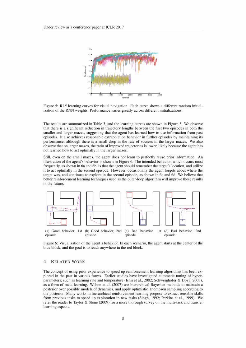
Figure 5: RL2 learning curves for visual navigation. Each curve shows a different random initial-ization of the RNN weights. Performance varies greatly across different initializations.

The results are summarized in Table 3, and the learning curves are shown in Figure 5. We observethat there is a significant reduction in trajectory lengths between the first two episodes in both thesmaller and larger mazes, suggesting that the agent has learned how to use information from pastepisodes. It also achieves reasonable extrapolation behavior in further episodes by maintaining itsperformance, although there is a small drop in the rate of success in the larger mazes. We alsoobserve that on larger mazes, the ratio of improved trajectories is lower, likely because the agent hasnot learned how to act optimally in the larger mazes.

Still, even on the small mazes, the agent does not learn to perfectly reuse prior information. Anillustration of the agent’s behavior is shown in Figure 6. The intended behavior, which occurs mostfrequently, as shown in 6a and 6b, is that the agent should remember the target’s location, and utilizeit to act optimally in the second episode. However, occasionally the agent forgets about where thetarget was, and continues to explore in the second episode, as shown in 6c and 6d. We believe thatbetter reinforcement learning techniques used as the outer-loop algorithm will improve these resultsin the future.

(a) Good behavior, 1stepisode

(b) Good behavior, 2ndepisode

(c) Bad behavior, 1stepisode

(d) Bad behavior, 2ndepisode

Figure 6: Visualization of the agent’s behavior. In each scenario, the agent starts at the center of theblue block, and the goal is to reach anywhere in the red block.

4 RELATED WORK

The concept of using prior experience to speed up reinforcement learning algorithms has been ex-plored in the past in various forms. Earlier studies have investigated automatic tuning of hyper-parameters, such as learning rate and temperature (Ishii et al., 2002; Schweighofer & Doya, 2003),as a form of meta-learning. Wilson et al. (2007) use hierarchical Bayesian methods to maintain aposterior over possible models of dynamics, and apply optimistic Thompson sampling according tothe posterior. Many works in hierarchical reinforcement learning propose to extract reusable skillsfrom previous tasks to speed up exploration in new tasks (Singh, 1992; Perkins et al., 1999). Werefer the reader to Taylor & Stone (2009) for a more thorough survey on the multi-task and transferlearning aspects.

8


More recently, Fu et al. (2015) propose a model-based approach on top of iLQG with unknowndynamics (Levine & Abbeel, 2014), which uses samples collected from previous tasks to builda neural network prior for the dynamics, and can perform one-shot learning on new, but relatedtasks thanks to reduced sample complexity. There has been a growing interest in using deep neuralnetworks for multi-task learning and transfer learning (Parisotto et al., 2015; Rusu et al., 2015;2016a; Devin et al., 2016; Rusu et al., 2016b).

In the broader context of machine learning, there has been a lot of interest in one-shot learningfor object classification (Vilalta & Drissi, 2002; Fei-Fei et al., 2006; Larochelle et al., 2008; Lakeet al., 2011; Koch, 2015). Our work draws inspiration from a particular line of work (Younger et al.,2001; Santoro et al., 2016; Vinyals et al., 2016), which formulates meta-learning as an optimizationproblem, and can thus be optimized end-to-end via gradient descent. While these work applies tothe supervised learning setting, our work applies in the more general reinforcement learning setting.Although the reinforcement learning setting is more challenging, the resulting behavior is far richer:our agent must not only learn to exploit existing information, but also learn to explore, a problemthat is usually not a factor in supervised learning. Another line of work (Hochreiter et al., 2001;Younger et al., 2001; Andrychowicz et al., 2016; Li & Malik, 2016) studies meta-learning over theoptimization process. There, the meta-learner makes explicit updates to a parametrized model. Incomparison, we do not use a directly parametrized policy; instead, the recurrent neural networkagent acts as the meta-learner and the resulting policy simultaneously.

Our formulation essentially constructs a partially observable MDP (POMDP) which is solved in theouter loop, where the underlying MDP is unobserved by the agent. This reduction of an unknownMDP to a POMDP can be traced back to dual control theory (Feldbaum, 1960), where “dual” refersto the fact that one is controlling both the state and the state estimate. Feldbaum pointed out thatthe solution can in principle be computed with dynamic programming, but doing so is usually im-practical. POMDPs with such structure have also been studied under the name “mixed observabilityMDPs” (Ong et al., 2010). However, the method proposed there suffers from the usual challengesof solving POMDPs in high dimensions.

5 DISCUSSION

This paper suggests a different approach for designing better reinforcement learning algorithms:instead of acting as the designers ourselves, learn the algorithm end-to-end using standard rein-forcement learning techniques. That is, the “fast” RL algorithm is a computation whose state isstored in the RNN activations, and the RNN’s weights are learned by a general-purpose “slow” re-inforcement learning algorithm. Our method, RL2, has demonstrated competence comparable withtheoretically optimal algorithms in small-scale settings. We have further shown its potential to scaleto high-dimensional tasks.

In the experiments, we have identified opportunities to improve upon RL2: the outer-loop reinforce-ment learning algorithm was shown to be an immediate bottleneck, and we believe that for settingswith extremely long horizons, better architecture may also be required for the policy. Although wehave used generic methods and architectures for the outer-loop algorithm and the policy, doing thisalso ignores the underlying episodic structure. We expect algorithms and policy architectures thatexploit the problem structure to significantly boost the performance.

ACKNOWLEDGMENTS

We would like to thank our colleagues at Berkeley and OpenAI for insightful discussions. Thisresearch was funded in part by ONR through a PECASE award. Yan Duan was also supported by aBerkeley AI Research lab Fellowship and a Huawei Fellowship. Xi Chen was also supported by aBerkeley AI Research lab Fellowship. We gratefully acknowledge the support of the NSF throughgrant IIS-1619362 and of the ARC through a Laureate Fellowship (FL110100281) and through theARC Centre of Excellence for Mathematical and Statistical Frontiers.

REFERENCES

Marcin Andrychowicz, Misha Denil, Sergio Gomez, Matthew W Hoffman, David Pfau, Tom Schaul,and Nando de Freitas. Learning to learn by gradient descent by gradient descent. arXiv preprint

9


arXiv:1606.04474, 2016.

Jean-Yves Audibert and Remi Munos. Introduction to bandits: Algorithms and theory. ICMLTutorial on bandits, 2011.

Peter Auer. Using confidence bounds for exploitation-exploration trade-offs. Journal of MachineLearning Research, 3(Nov):397–422, 2002.

Yoshua Bengio, Patrice Simard, and Paolo Frasconi. Learning long-term dependencies with gradientdescent is difficult. IEEE transactions on neural networks, 5(2):157–166, 1994.

Sebastien Bubeck and Nicolo Cesa-Bianchi. Regret analysis of stochastic and nonstochastic multi-armed bandit problems. arXiv preprint arXiv:1204.5721, 2012.

Jhelum Chakravorty and Aditya Mahajan. Multi-armed bandits, gittins index, and its calculation.Methods and Applications of Statistics in Clinical Trials: Planning, Analysis, and InferentialMethods, 2:416–435, 2013.

Olivier Chapelle and Lihong Li. An empirical evaluation of thompson sampling. In Advances inneural information processing systems, pp. 2249–2257, 2011.

Kyunghyun Cho, Bart Van Merrienboer, Dzmitry Bahdanau, and Yoshua Bengio. On the propertiesof neural machine translation: Encoder-decoder approaches. arXiv preprint arXiv:1409.1259,2014.

Junyoung Chung, Caglar Gulcehre, KyungHyun Cho, and Yoshua Bengio. Empirical evaluation ofgated recurrent neural networks on sequence modeling. arXiv preprint arXiv:1412.3555, 2014.

Marc Deisenroth and Carl E Rasmussen. Pilco: A model-based and data-efficient approach to policysearch. In Proceedings of the 28th International Conference on machine learning (ICML-11), pp.465–472, 2011.

Coline Devin, Abhishek Gupta, Trevor Darrell, Pieter Abbeel, and Sergey Levine. Learning modularneural network policies for multi-task and multi-robot transfer. arXiv preprint arXiv:1609.07088,2016.

Li Fei-Fei, Rob Fergus, and Pietro Perona. One-shot learning of object categories. IEEE transactionson pattern analysis and machine intelligence, 28(4):594–611, 2006.

AA Feldbaum. Dual control theory. i. Avtomatika i Telemekhanika, 21(9):1240–1249, 1960.

Justin Fu, Sergey Levine, and Pieter Abbeel. One-shot learning of manipulation skills with onlinedynamics adaptation and neural network priors. arXiv preprint arXiv:1509.06841, 2015.

Mohammad Ghavamzadeh, Shie Mannor, Joelle Pineau, Aviv Tamar, et al. Bayesian reinforcementlearning: a survey. World Scientific, 2015.

John Gittins, Kevin Glazebrook, and Richard Weber. Multi-armed bandit allocation indices. JohnWiley & Sons, 2011.

John C Gittins. Bandit processes and dynamic allocation indices. Journal of the Royal StatisticalSociety. Series B (Methodological), pp. 148–177, 1979.

Xiaoxiao Guo, Satinder Singh, Honglak Lee, Richard L Lewis, and Xiaoshi Wang. Deep learningfor real-time atari game play using offline monte-carlo tree search planning. In Advances in neuralinformation processing systems, pp. 3338–3346, 2014.

Nicolas Heess, Gregory Wayne, David Silver, Tim Lillicrap, Tom Erez, and Yuval Tassa. Learningcontinuous control policies by stochastic value gradients. In Advances in Neural InformationProcessing Systems, pp. 2944–2952, 2015.

Sepp Hochreiter, A Steven Younger, and Peter R Conwell. Learning to learn using gradient descent.In International Conference on Artificial Neural Networks, pp. 87–94. Springer, 2001.

10


Shin Ishii, Wako Yoshida, and Junichiro Yoshimoto. Control of exploitation–exploration meta-parameter in reinforcement learning. Neural networks, 15(4):665–687, 2002.

Thomas Jaksch, Ronald Ortner, and Peter Auer. Near-optimal regret bounds for reinforcementlearning. Journal of Machine Learning Research, 11(Apr):1563–1600, 2010.

Rafal Jozefowicz, Wojciech Zaremba, and Ilya Sutskever. An empirical exploration of recur-rent network architectures. In Proceedings of the 32nd International Conference on MachineLearning, ICML 2015, Lille, France, 6-11 July 2015, pp. 2342–2350, 2015. URL http://jmlr.org/proceedings/papers/v37/jozefowicz15.html.

Michał Kempka, Marek Wydmuch, Grzegorz Runc, Jakub Toczek, and Wojciech Jaskowski. Viz-doom: A doom-based ai research platform for visual reinforcement learning. arXiv preprintarXiv:1605.02097, 2016.

Gregory Koch. Siamese neural networks for one-shot image recognition. PhD thesis, University ofToronto, 2015.

J Zico Kolter and Andrew Y Ng. Near-bayesian exploration in polynomial time. In Proceedings ofthe 26th Annual International Conference on Machine Learning, pp. 513–520. ACM, 2009.

Brenden M Lake, Ruslan Salakhutdinov, Jason Gross, and Joshua B Tenenbaum. One shot learningof simple visual concepts. In Proceedings of the 33rd Annual Conference of the Cognitive ScienceSociety, volume 172, pp. 2, 2011.

Hugo Larochelle, Dumitru Erhan, and Yoshua Bengio. Zero-data learning of new tasks. In AAAI,volume 1, pp. 3, 2008.

Sergey Levine and Pieter Abbeel. Learning neural network policies with guided policy search underunknown dynamics. In Advances in Neural Information Processing Systems, pp. 1071–1079,2014.

Sergey Levine, Chelsea Finn, Trevor Darrell, and Pieter Abbeel. End-to-end training of deep visuo-motor policies. Journal of Machine Learning Research, 17(39):1–40, 2016.

Ke Li and Jitendra Malik. Learning to optimize. arXiv preprint arXiv:1606.01885, 2016.

Timothy P Lillicrap, Jonathan J Hunt, Alexander Pritzel, Nicolas Heess, Tom Erez, Yuval Tassa,David Silver, and Daan Wierstra. Continuous control with deep reinforcement learning. arXivpreprint arXiv:1509.02971, 2015.

Benedict C May, Nathan Korda, Anthony Lee, and David S Leslie. Optimistic bayesian sampling incontextual-bandit problems. Journal of Machine Learning Research, 13(Jun):2069–2106, 2012.

Volodymyr Mnih, Koray Kavukcuoglu, David Silver, Andrei A Rusu, Joel Veness, Marc G Belle-mare, Alex Graves, Martin Riedmiller, Andreas K Fidjeland, Georg Ostrovski, et al. Human-levelcontrol through deep reinforcement learning. Nature, 518(7540):529–533, 2015.

Junhyuk Oh, Valliappa Chockalingam, Satinder Singh, and Honglak Lee. Control of memory, activeperception, and action in minecraft. arXiv preprint arXiv:1605.09128, 2016.

Sylvie CW Ong, Shao Wei Png, David Hsu, and Wee Sun Lee. Planning under uncertainty forrobotic tasks with mixed observability. The International Journal of Robotics Research, 29(8):1053–1068, 2010.

Ian Osband and Benjamin Van Roy. Why is posterior sampling better than optimism for reinforce-ment learning. arXiv preprint arXiv:1607.00215, 2016.

Ian Osband, Dan Russo, and Benjamin Van Roy. (more) efficient reinforcement learning via poste-rior sampling. In Advances in Neural Information Processing Systems, pp. 3003–3011, 2013.

Emilio Parisotto, Jimmy Lei Ba, and Ruslan Salakhutdinov. Actor-mimic: Deep multitask andtransfer reinforcement learning. arXiv preprint arXiv:1511.06342, 2015.

11


Theodore J Perkins, Doina Precup, et al. Using options for knowledge transfer in reinforcementlearning. University of Massachusetts, Amherst, MA, USA, Tech. Rep, 1999.

Andrei A Rusu, Sergio Gomez Colmenarejo, Caglar Gulcehre, Guillaume Desjardins, James Kirk-patrick, Razvan Pascanu, Volodymyr Mnih, Koray Kavukcuoglu, and Raia Hadsell. Policy distil-lation. arXiv preprint arXiv:1511.06295, 2015.

Andrei A Rusu, Neil C Rabinowitz, Guillaume Desjardins, Hubert Soyer, James Kirkpatrick, KorayKavukcuoglu, Razvan Pascanu, and Raia Hadsell. Progressive neural networks. arXiv preprintarXiv:1606.04671, 2016a.

Andrei A Rusu, Matej Vecerik, Thomas Rothorl, Nicolas Heess, Razvan Pascanu, and Raia Hadsell.Sim-to-real robot learning from pixels with progressive nets. arXiv preprint arXiv:1610.04286,2016b.

Adam Santoro, Sergey Bartunov, Matthew Botvinick, Daan Wierstra, and Timothy Lillicrap. One-shot learning with memory-augmented neural networks. arXiv preprint arXiv:1605.06065, 2016.

John Schulman, Sergey Levine, Philipp Moritz, Michael I Jordan, and Pieter Abbeel. Trust regionpolicy optimization. CoRR, abs/1502.05477, 2015.

John Schulman, Philipp Moritz, Sergey Levine, Michael Jordan, and Pieter Abbeel. High-dimensional continuous control using generalized advantage estimation. In International Con-ference on Learning Representations (ICLR2016), 2016.

Nicolas Schweighofer and Kenji Doya. Meta-learning in reinforcement learning. Neural Networks,16(1):5–9, 2003.

Satinder Pal Singh. Transfer of learning by composing solutions of elemental sequential tasks.Machine Learning, 8(3-4):323–339, 1992.

Malcolm Strens. A bayesian framework for reinforcement learning. In ICML, pp. 943–950, 2000.

Matthew E Taylor and Peter Stone. Transfer learning for reinforcement learning domains: A survey.Journal of Machine Learning Research, 10(Jul):1633–1685, 2009.

William R Thompson. On the likelihood that one unknown probability exceeds another in view ofthe evidence of two samples. Biometrika, 25(3/4):285–294, 1933.

Ricardo Vilalta and Youssef Drissi. A perspective view and survey of meta-learning. ArtificialIntelligence Review, 18(2):77–95, 2002.

Oriol Vinyals, Charles Blundell, Timothy Lillicrap, Koray Kavukcuoglu, and Daan Wierstra. Match-ing networks for one shot learning. arXiv preprint arXiv:1606.04080, 2016.

Niklas Wahlstrom, Thomas B Schon, and Marc Peter Deisenroth. From pixels to torques: Policylearning with deep dynamical models. arXiv preprint arXiv:1502.02251, 2015.

Manuel Watter, Jost Springenberg, Joschka Boedecker, and Martin Riedmiller. Embed to control:A locally linear latent dynamics model for control from raw images. In Advances in NeuralInformation Processing Systems, pp. 2746–2754, 2015.

Peter Whittle. Optimization over time. John Wiley & Sons, Inc., 1982.

Aaron Wilson, Alan Fern, Soumya Ray, and Prasad Tadepalli. Multi-task reinforcement learning: ahierarchical bayesian approach. In Proceedings of the 24th international conference on Machinelearning, pp. 1015–1022. ACM, 2007.

A Steven Younger, Sepp Hochreiter, and Peter R Conwell. Meta-learning with backpropagation. InNeural Networks, 2001. Proceedings. IJCNN’01. International Joint Conference on, volume 3.IEEE, 2001.

12


APPENDIX

A DETAILED EXPERIMENT SETUP

Common to all experiments: as mentioned in Section 2.2, we use placeholder values when neces-sary. For example, at t = 0 there is no previous action, reward, or termination flag. Since all ofour experiments use discrete actions, we use the embedding of the action 0 as a placeholder foractions, and 0 for both the rewards and termination flags. To form the input to the GRU, we usethe values for the rewards and termination flags as-is, and embed the states and actions as describedseparately below for each experiments. These values are then concatenated together to form the jointembedding.

For the neural network architecture, We use rectified linear units throughout the experiments as thehidden activation, and we apply weight normalization without data-dependent initialization (Sali-mans & Kingma, 2016) to all weight matrices. The hidden-to-hidden weight matrix uses an orthog-onal initialization (Saxe et al., 2013), and all other weight matrices use Xavier initialization (Glorot& Bengio, 2010). We initialize all bias vectors to 0. Unless otherwise mentioned, the policy andthe baseline uses separate neural networks with the same architecture until the final layer, where thenumber of outputs differ.

All experiments are implemented using TensorFlow (Abadi et al., 2016) and rllab (Duan et al.,2016). We use the implementations of classic algorithms provided by the TabulaRL package (Os-band, 2016).

A.1 MULTI-ARMED BANDITS

The parameters for TRPO are shown in Table 1. Since the environment is stateless, we use a constantembedding 0 as a placeholder in place of the states, and a one-hot embedding for the actions.

Table 1: Hyperparameters for TRPO: multi-armed bandits

Discount 0.99GAE λ 0.3Policy Iters Up to 1000#GRU Units 256Mean KL 0.01Batch size 250000

A.2 TABULAR MDPS

The parameters for TRPO are shown in Table 2. We use a one-hot embedding for the states andactions separately, which are then concatenated together.

Table 2: Hyperparameters for TRPO: tabular MDPs


A.3 VISUAL NAVIGATION

The parameters for TRPO are shown in Table 3. For this task, we use a neural network to formthe joint embedding. We rescale the images to have width 40 and height 30 with RGB channelspreserved, and we recenter the RGB values to lie within range [−1, 1]. Then, this preprocessed

13


image is passed through 2 convolution layers, each with 16 filters of size 5 × 5 and stride 2. Theaction is first embedded into a 256-dimensional vector where the embedding is learned, and thenconcatenated with the flattened output of the final convolution layer. The joint vector is then fed toa fully connected layer with 256 hidden units.

Unlike previous experiments, we let the policy and the baseline share the same neural network. Wefound this to improve the stability of training baselines and also the end performance of the policy,possibly due to regularization effects and better learned features imposed by weight sharing. Similarweight-sharing techniques have also been explored in (Mnih et al., 2016).

Table 3: Hyperparameters for TRPO: visual navigation


REFERENCES

Martın Abadi, Ashish Agarwal, Paul Barham, Eugene Brevdo, Zhifeng Chen, Craig Citro, Greg SCorrado, Andy Davis, Jeffrey Dean, Matthieu Devin, et al. Tensorflow: Large-scale machinelearning on heterogeneous distributed systems. arXiv preprint arXiv:1603.04467, 2016.

Yan Duan, Xi Chen, Rein Houthooft, John Schulman, and Pieter Abbeel. Benchmarking deepreinforcement learning for continuous control. arXiv preprint arXiv:1604.06778, 2016.

Xavier Glorot and Yoshua Bengio. Understanding the difficulty of training deep feedforward neuralnetworks. In Aistats, volume 9, pp. 249–256, 2010.

Volodymyr Mnih, Adria Puigdomenech Badia, Mehdi Mirza, Alex Graves, Timothy P Lillicrap, TimHarley, David Silver, and Koray Kavukcuoglu. Asynchronous methods for deep reinforcementlearning. arXiv preprint arXiv:1602.01783, 2016.

Ian Osband. TabulaRL. https://github.com/iosband/TabulaRL, 2016.

Tim Salimans and Diederik P Kingma. Weight normalization: A simple reparameterization to ac-celerate training of deep neural networks. arXiv preprint arXiv:1602.07868, 2016.

Andrew M Saxe, James L McClelland, and Surya Ganguli. Exact solutions to the nonlinear dynam-ics of learning in deep linear neural networks. arXiv preprint arXiv:1312.6120, 2013.

14

Documents

Under review as a conference paper at ICLR 2017 · Under review as a conference paper at ICLR 2017 RL 2: FAST R EINFORCEMENT L EARNING VIA S LOW R EINFORCEMENT L EARNING Yan Duan