Embed Size (px)
Citation preview
Understanding Basic Statistics
Chapter Seven
Normal Distributions
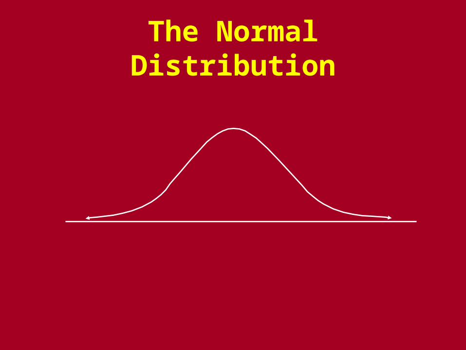
The Normal Distribution
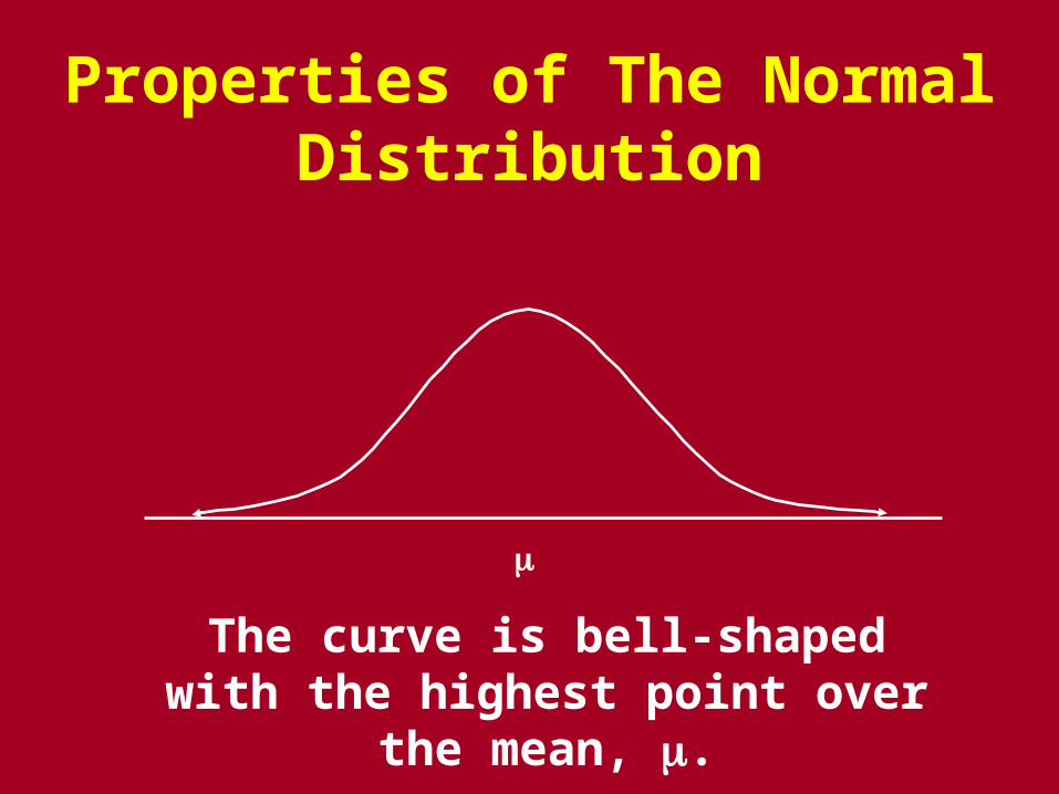
Properties of The Normal Distribution
The curve is bell-shaped with the highest point over the mean, .
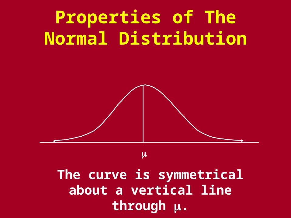
Properties of The Normal Distribution
The curve is symmetrical about a vertical line through .
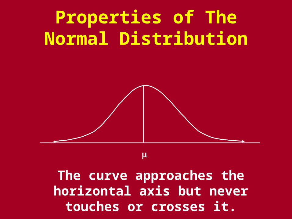
Properties of The Normal Distribution
The curve approaches the horizontal axis but never touches
or crosses it.
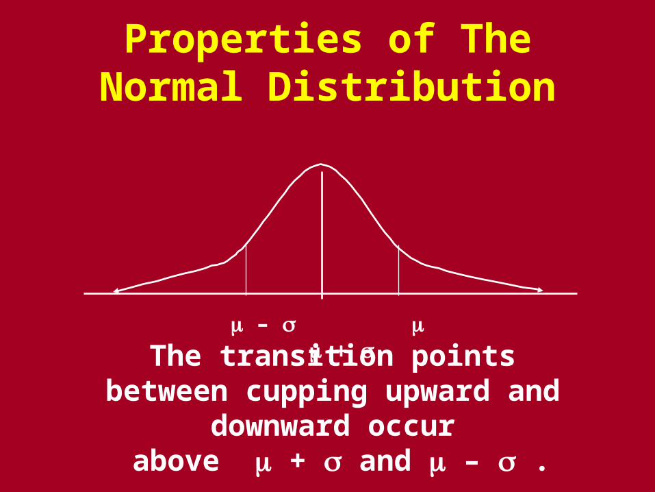
Properties of The Normal Distribution
The transition points between cupping upward and downward
occur above + and – .
–
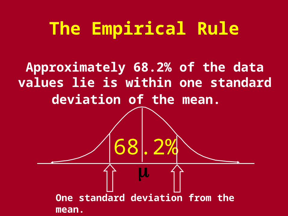
The Empirical Rule
Approximately 68.2% of the data values lie is within one standard deviation of the
mean.
One standard deviation from the mean.
68.2%
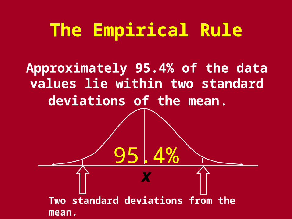
The Empirical RuleThe Empirical Rule
Approximately 95.4% of the data values lie within two standard deviations of the mean.
Two standard deviations from the mean.
x95.4%
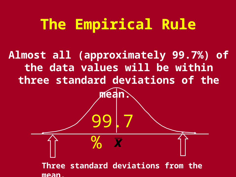
The Empirical RuleThe Empirical Rule
Almost all (approximately 99.7%) of the data values will be within three standard
deviations of the mean.
Three standard deviations from the mean.
x99.7%

Application of the Empirical Rule
The life of a particular type of lightbulb is normally distributed with
a mean of 1100 hours and a standard deviation of 100 hours.
• What is the probability that a lightbulb of this type will last between 1000 and 1200 hours?
Approximately 68.2%

Control Chart
a statistical tool to track data over a period of equally spaced time intervals or in
some sequential order
Statistical Control
A random variable is in statistical control if it can be
described by the same probability distribution when it is observed at
successive points in time.

To Construct a Control Chart• Draw a center horizontal line at .• Draw dashed lines (control limits) at
and .• The values of and s may be target
values or may be computed from past data when the process was in control.
• Plot the variable being measured using time on the horizontal axis.
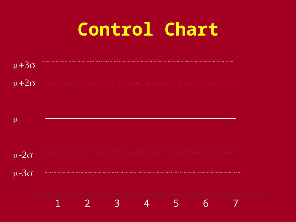
Control Chart
1 2 3 4 5 6 7
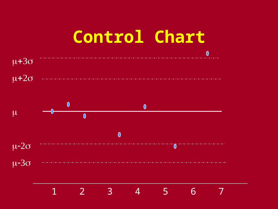
Control Chart
1 2 3 4 5 6 7

Out-Of-Control Warning Signals
I One point beyond the 3 level
II A run of nine consecutive points on one side of the center line
III At least two of three consecutive points beyond the 2 level on the same side of the center line.
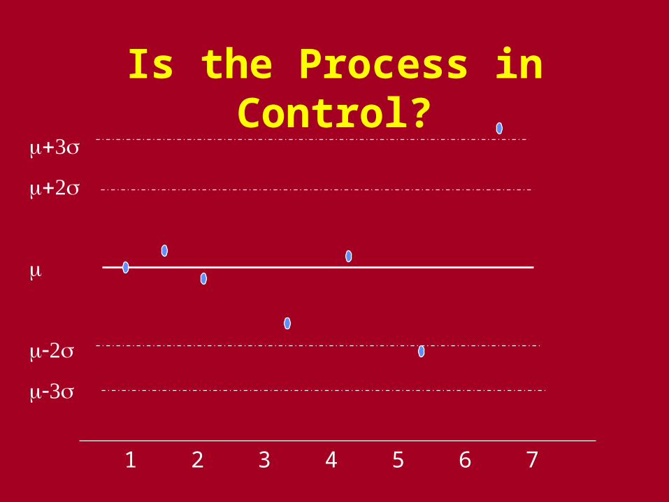
Is the Process in Control?
1 2 3 4 5 6 7
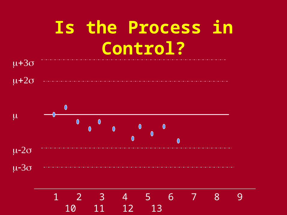
Is the Process in Control?
1 2 3 4 5 6 7 8 9 10 11 12 13

Is the Process in Control?
1 2 3 4 5 6 7
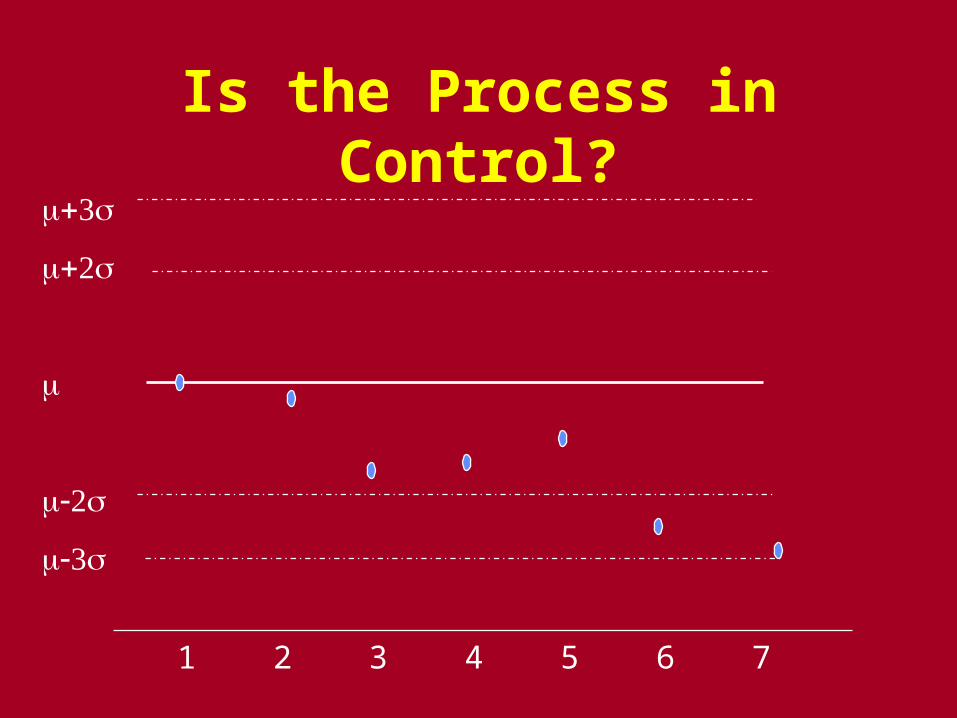
Is the Process in Control?
1 2 3 4 5 6 7
Z Score
• The z value or z score tells the number of standard deviations the original measurement is from the mean.
• The z value is in standard units.
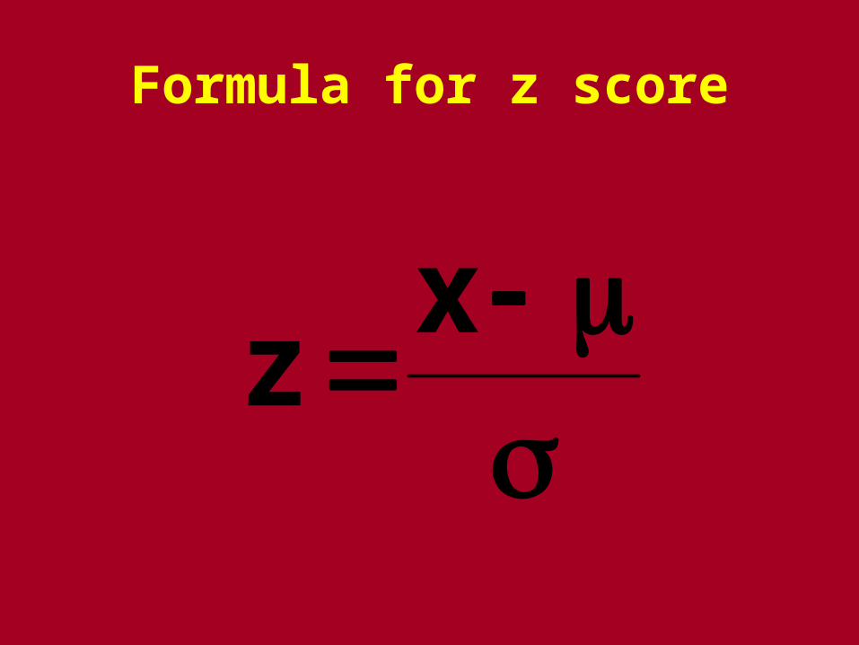
Formula for z score
x
z
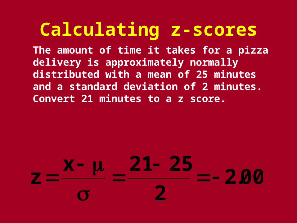
Calculating z-scoresThe amount of time it takes for a pizza delivery is approximately normally distributed with a mean of 25 minutes and a standard deviation of 2 minutes. Convert 21 minutes to a z score.
00.22
2521xz
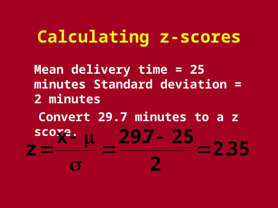
Calculating z-scores
Mean delivery time = 25 minutes Standard deviation = 2 minutes
Convert 29.7 minutes to a z score.
35.22
257.29xz
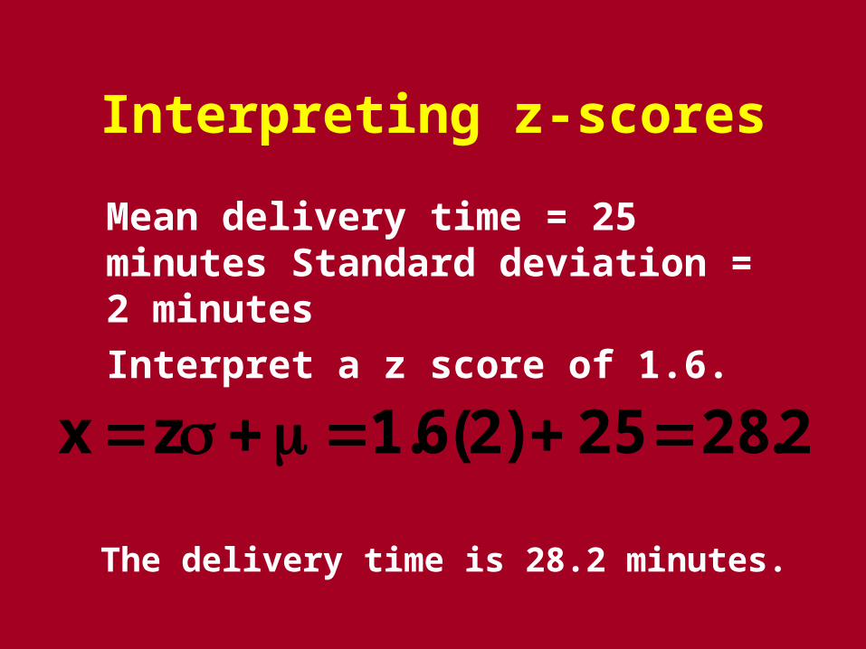
Interpreting z-scores
Mean delivery time = 25 minutes Standard deviation = 2 minutes
Interpret a z score of 1.6.
2.2825)2(6.1zx
The delivery time is 28.2 minutes.
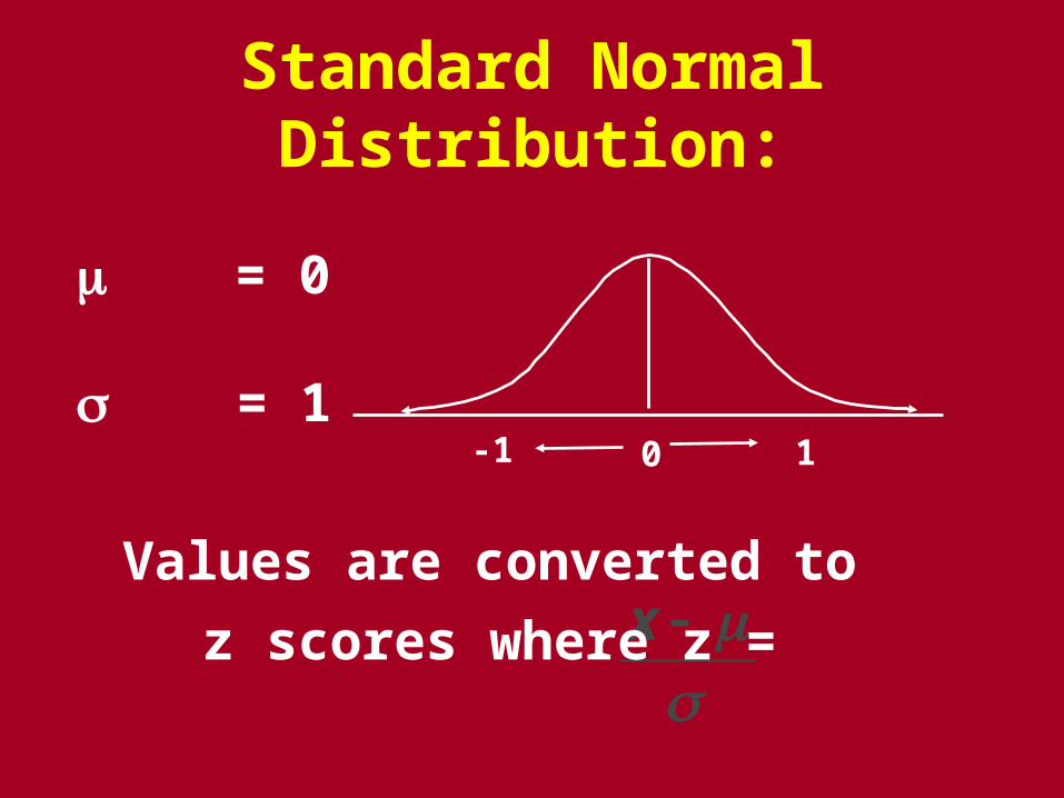
Standard Normal Distribution:
= 0
= 1
x
-1 1
Values are converted to
z scores where z =
0
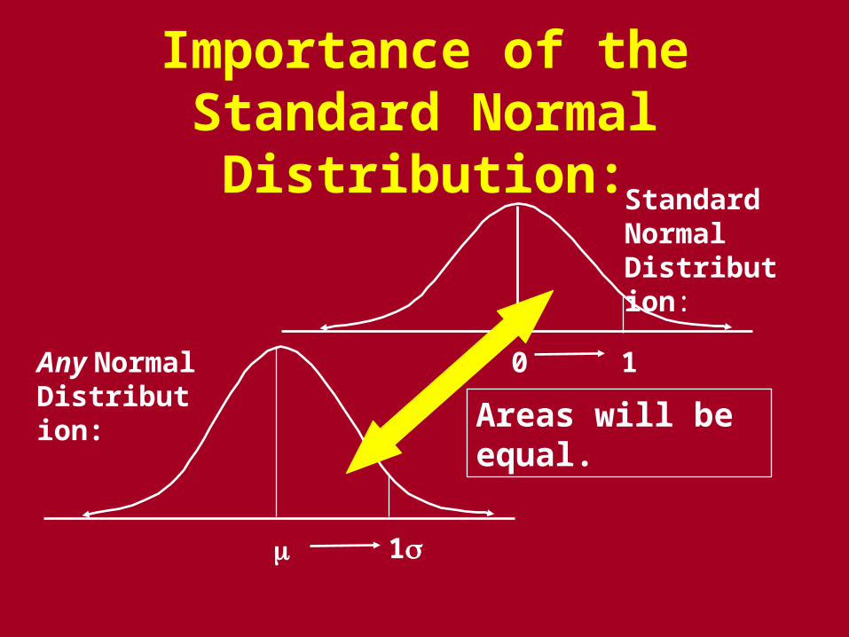
Importance of the Standard Normal Distribution:
10
1
Areas will be equal.
Any Normal Distribution:
Standard Normal Distribution:
Use of the Normal Probability Table
(Table 4) - Appendix I
Entries give the probability that a standard normally
distributed random variable will assume a value between the mean (zero) and a given
z-score.
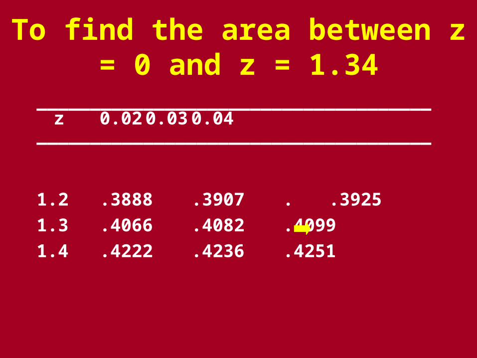
To find the area between z = 0 and z = 1.34
_____________________________________z0.02 0.03 0.04
_____________________________________
1.2 .3888 .3907. .3925
1.3 .4066 .4082 .4099
1.4 .4222 .4236 .4251
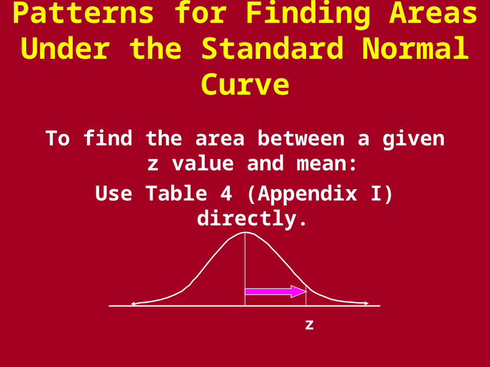
Patterns for Finding Areas Under the Standard Normal Curve
To find the area between a given z value and mean:
Use Table 4 (Appendix I) directly.
z
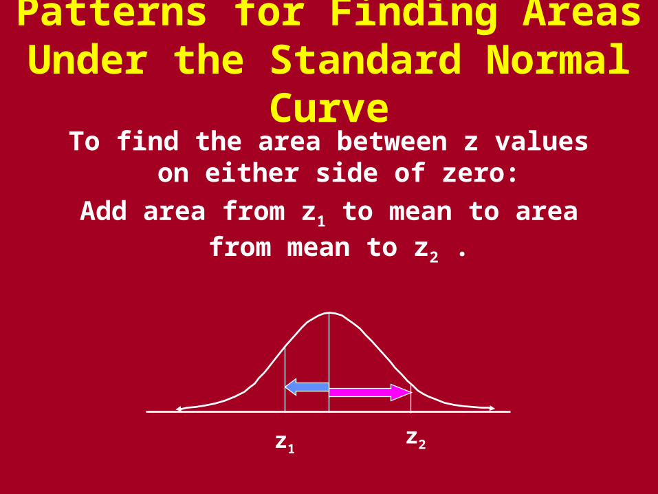
Patterns for Finding Areas Under the Standard Normal Curve
To find the area between z values on either side of zero:
Add area from z1 to mean to area from mean to z2 .
z2z1
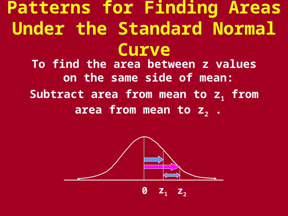
Patterns for Finding Areas Under the Standard Normal CurveTo find the area between z values on the
same side of mean:
Subtract area from mean to z1 from area from mean to z2 .
z20 z1
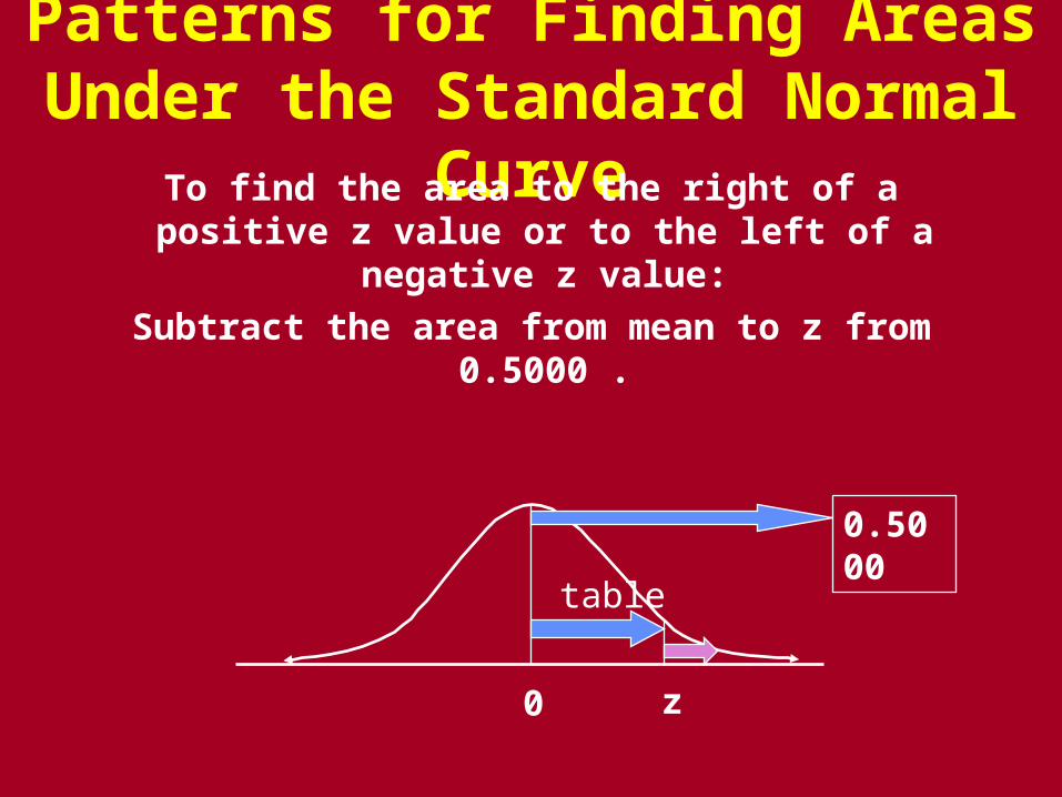
Patterns for Finding Areas Under the Standard Normal Curve
To find the area to the right of a positive z value or to the left of a negative z value:
Subtract the area from mean to z from 0.5000 .
z0
0.5000
table
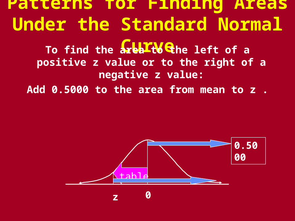
Patterns for Finding Areas Under the Standard Normal CurveTo find the area to the left of a positive z
value or to the right of a negative z value:
Add 0.5000 to the area from mean to z .
z 0
0.5000
table
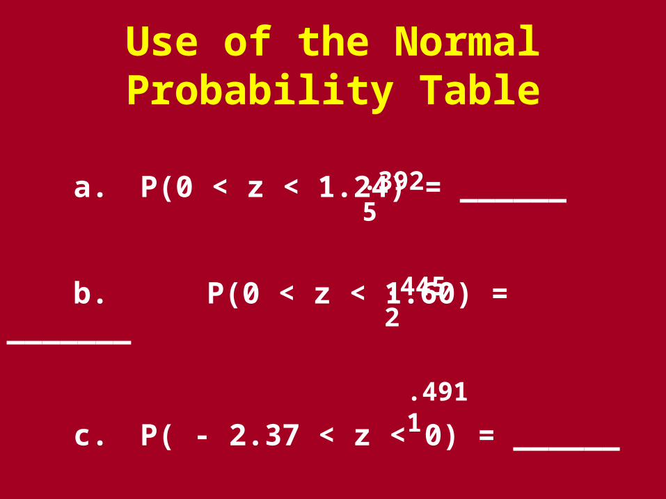
Use of the Normal Probability Table
a. P(0 < z < 1.24) = ______
b. P(0 < z < 1.60) = _______
c. P( - 2.37 < z < 0) = ______
.3925
.4452
.4911
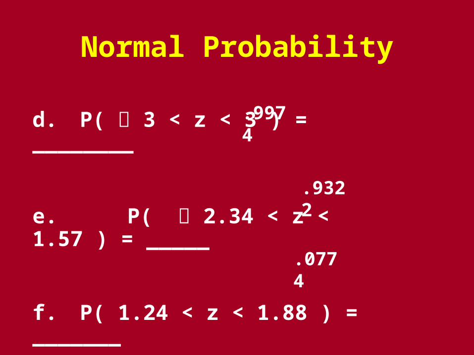
Normal Probability
d. P( 3 < z < 3 ) = ________
e. P( 2.34 < z < 1.57 ) = _____
f. P( 1.24 < z < 1.88 ) = _______
.9974
.9322
.0774
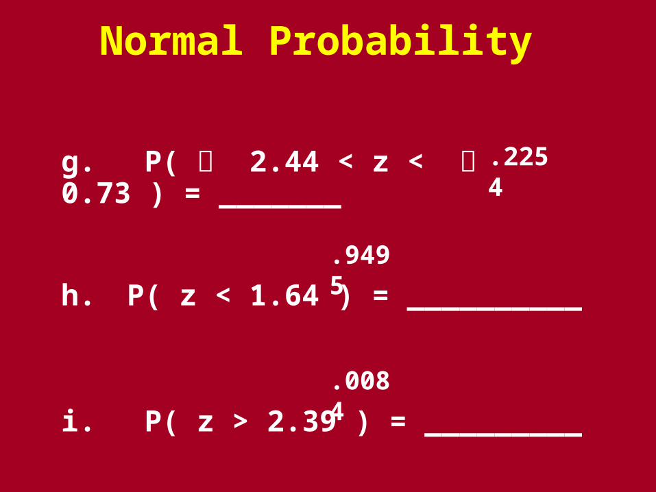
Normal Probability
g. P( 2.44 < z < 0.73 ) = _______
h. P( z < 1.64 ) = __________
i. P( z > 2.39 ) = _________
.9495
.0084
.2254
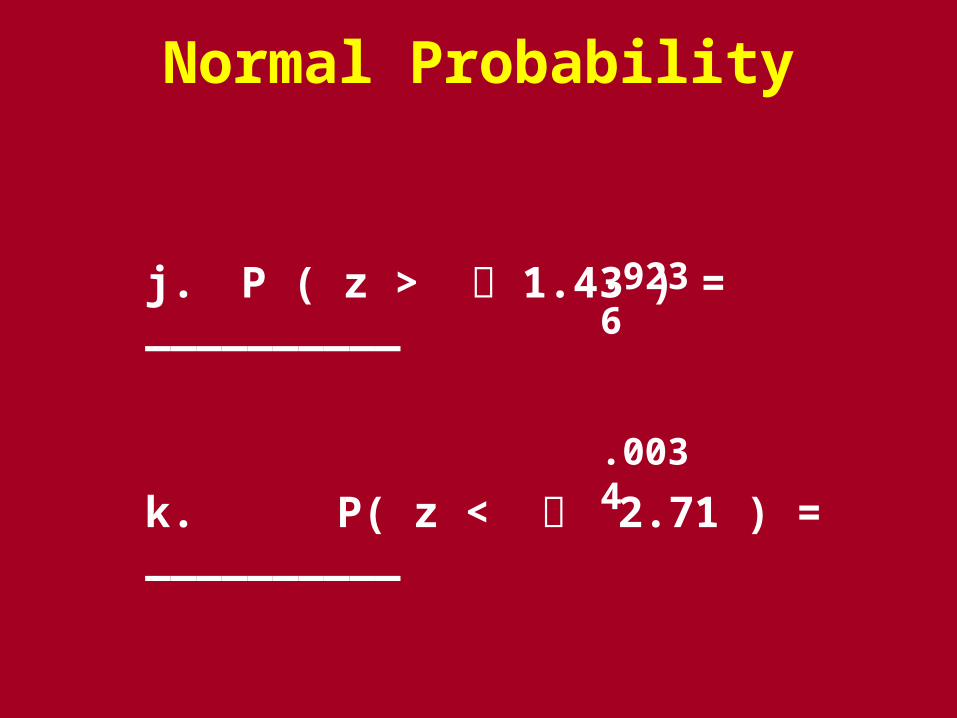
Normal Probability
j. P ( z > 1.43 ) = __________
k. P( z < 2.71 ) = __________
.9236
.0034
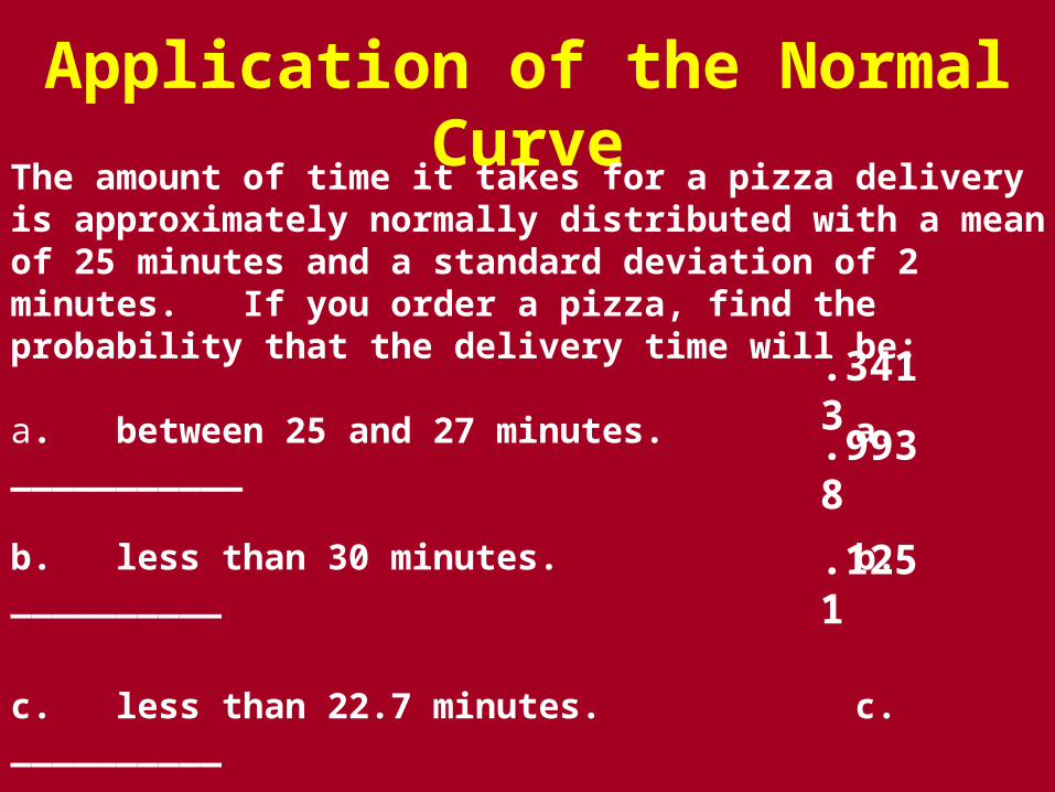
Application of the Normal CurveThe amount of time it takes for a pizza delivery is approximately normally distributed with a mean of 25 minutes and a standard deviation of 2 minutes. If you order a pizza, find the probability that the delivery time will be:
a. between 25 and 27 minutes. a. ___________
b. less than 30 minutes. b. __________
c. less than 22.7 minutes. c. __________
.3413
.9938
.1251
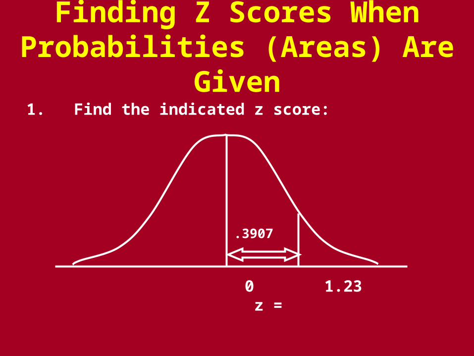
Finding Z Scores When Probabilities (Areas) Are Given1. Find the indicated z score:
.3907
0 z = 1.23
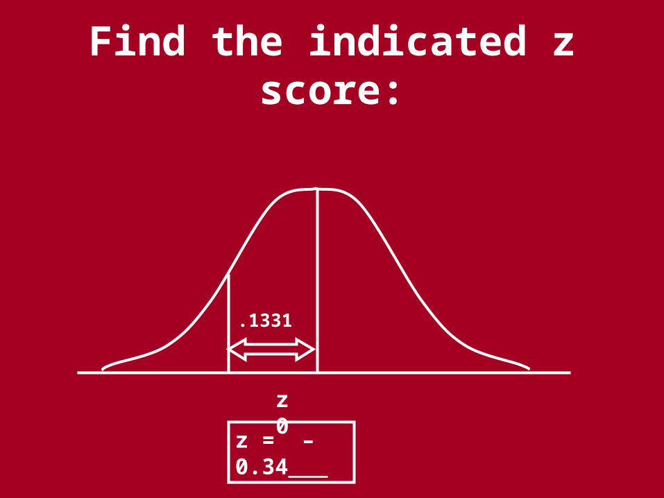
Find the indicated z score:
.1331
z 0
z = – 0.34
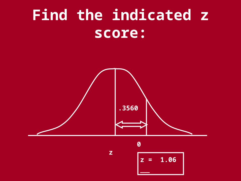
Find the indicated z score:
.3560
0 z
z = 1.06
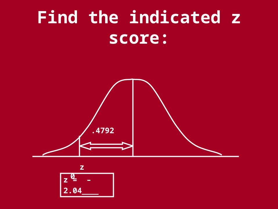
Find the indicated z score:
.4792
z 0
z = – 2.04
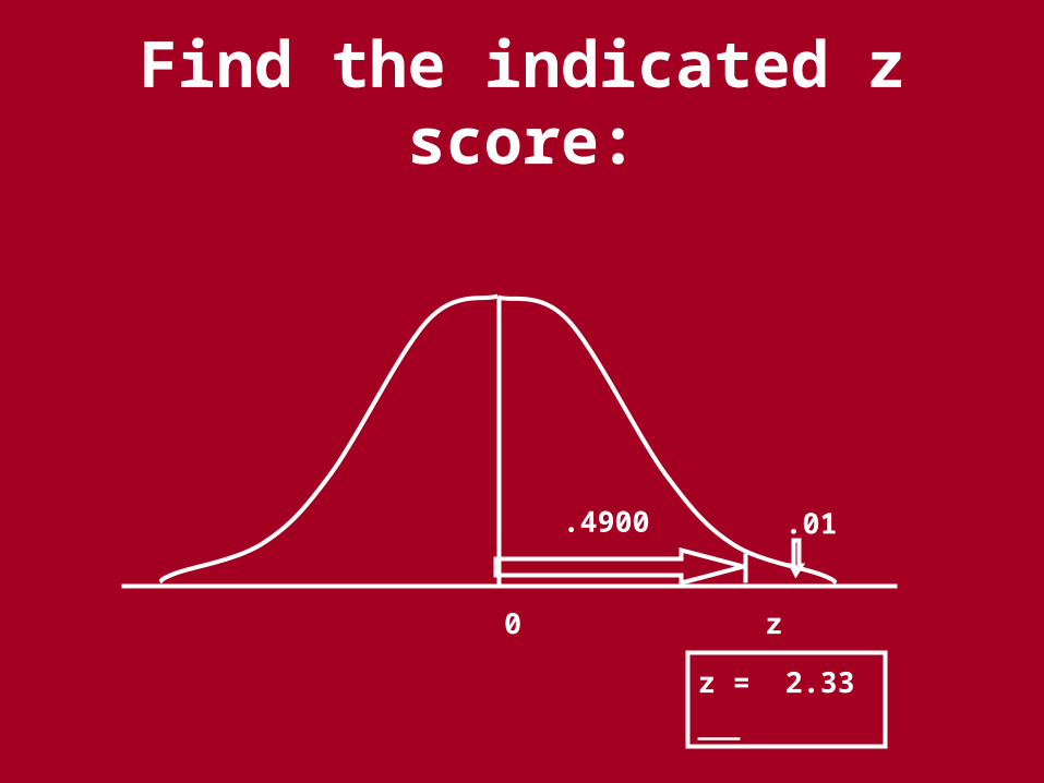
Find the indicated z score:
z = 2.33
.01
0 z
.4900
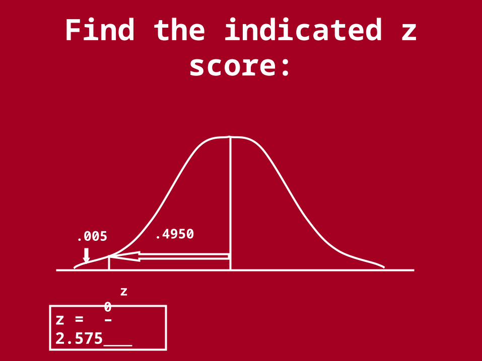
Find the indicated z score:
z = – 2.575
z 0
.005 .4950
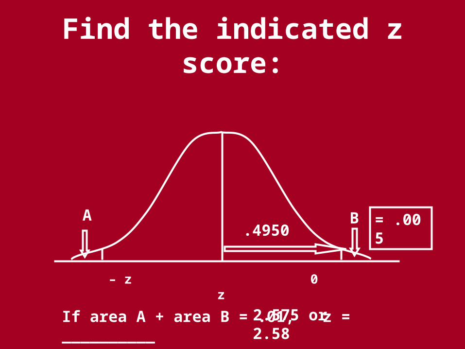
Find the indicated z score:
If area A + area B = .01, z = __________
A B
– z 0 z
2.575 or 2.58
= .005.4950
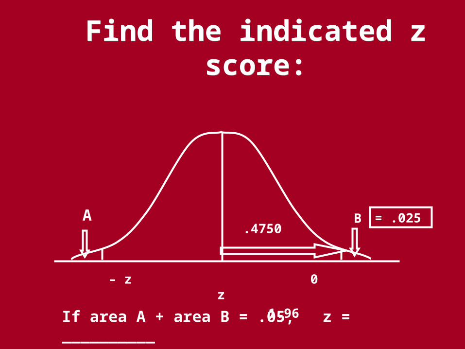
Find the indicated z score:Find the indicated z score:
If area A + area B = .05, z = __________
A B
– z 0 z
1.96
= .025.4750

Application of Determining z Scores
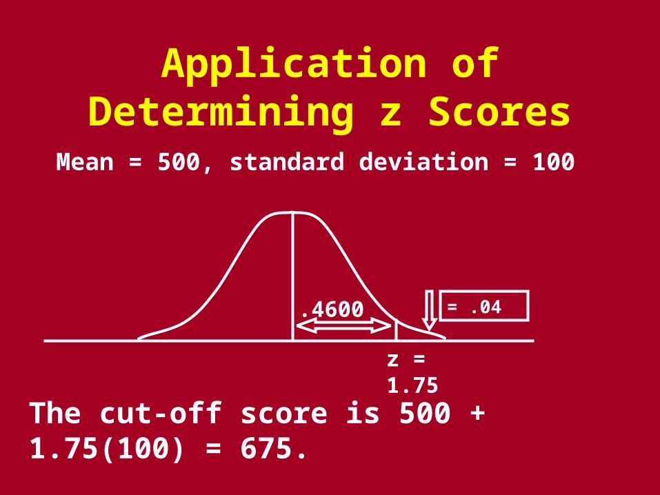
The Verbal SAT test has a mean score of 500 and a standard deviation of 100. Scores are normally distributed. A major university determines that it will accept only students whose Verbal SAT scores are in the top 4%. What is the minimum score that a student must earn to be accepted?

Application of Determining z Scores
Mean = 500, standard deviation = 100
= .04.4600
z = 1.75
The cut-off score is 1.75 standard deviations above the mean.
Application of Determining z Scores
Mean = 500, standard deviation = 100
= .04.4600
z = 1.75
The cut-off score is 500 + 1.75(100) = 675.

Normal Approximation Of The Binomial Distribution:
If n (the number of trials) is sufficiently large, a binomial
random variable has a distribution that is
approximately normal.

Define “sufficiently large”
The sample size, n, is considered to be
"sufficiently large" if np and nq
are both greater than 5.

Mean and Standard Deviation: Binomial
Distribution
qpnandpn
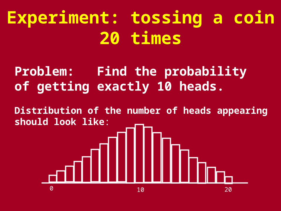
Experiment: tossing a coin 20 times
Problem: Find the probability of getting exactly 10 heads.
Distribution of the number of heads appearing should look like:
10 200
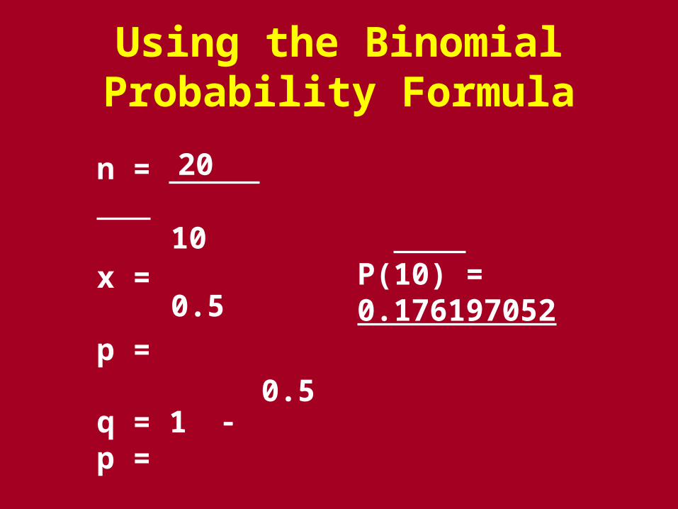
Using the Binomial Probability Formula
n =
x =
p =
q = 1 p =
P(10) = 0.176197052
20
10
0.5
0.5
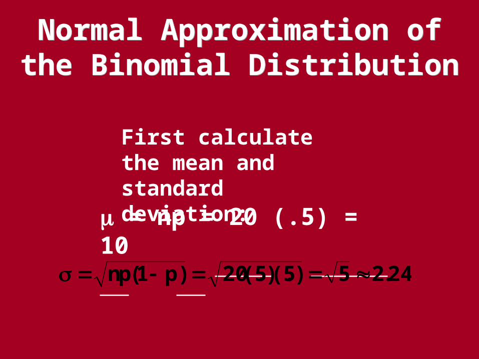
Normal Approximation of the Binomial Distribution
Normal Approximation of the Binomial Distribution
First calculate the mean and standard deviation:
= np = 20 (.5) = 10
24.25)5(.)5(.20)p1(pn
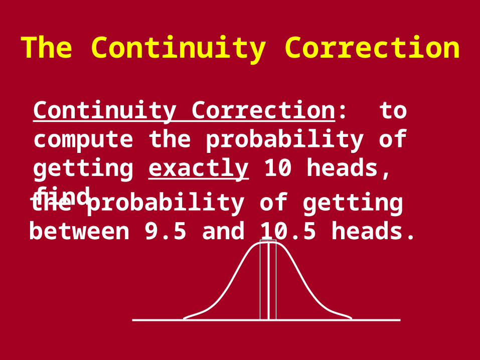
The Continuity Correction
Continuity Correction: to compute the probability of getting exactly 10 heads, find the probability of getting between 9.5 and 10.5 heads.
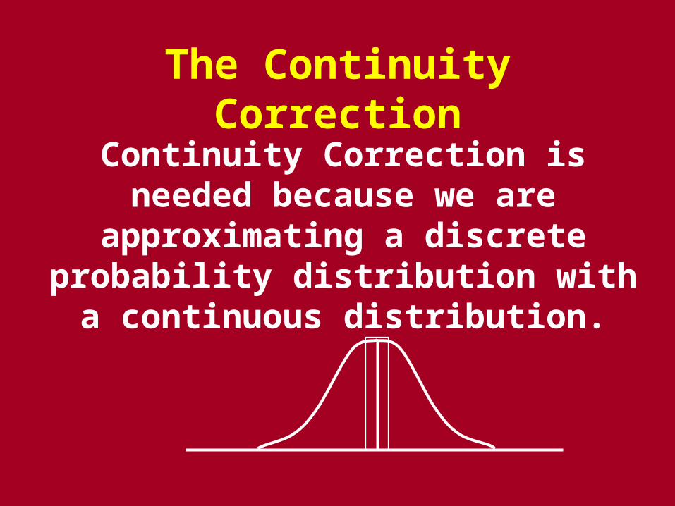
The Continuity Correction
Continuity Correction is needed because we are approximating a
discrete probability distribution with a continuous distribution.
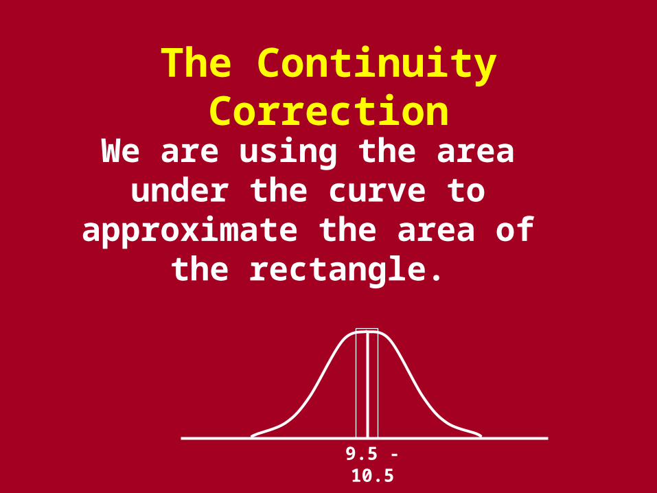
The Continuity Correction
We are using the area under the curve to approximate the area of
the rectangle.
9.5 - 10.5
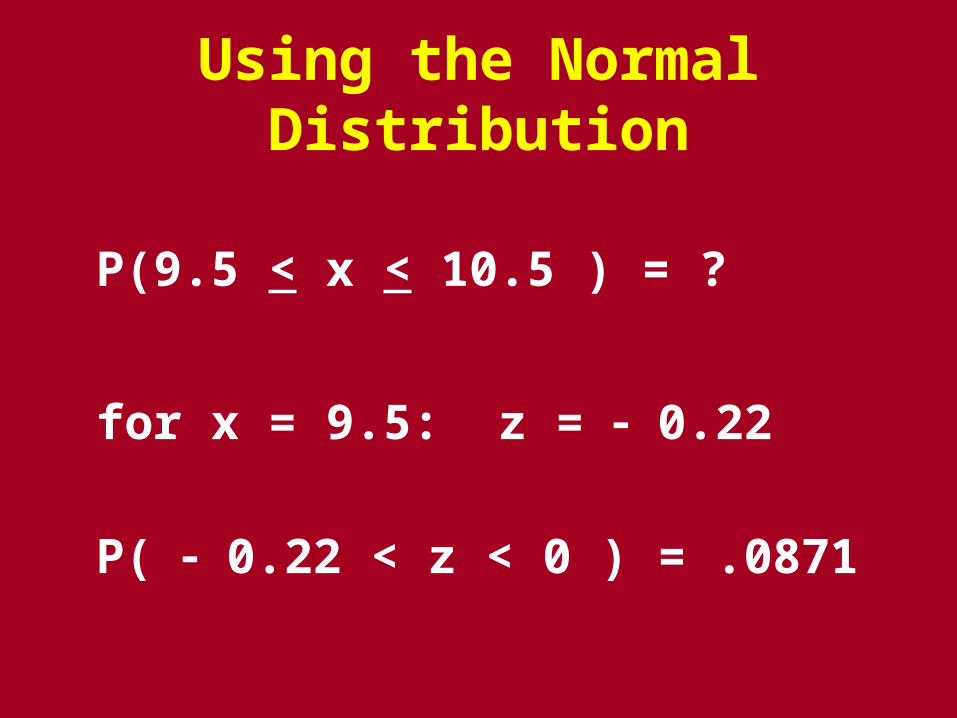
Using the Normal Distribution
P(9.5 < x < 10.5 ) = ?
for x = 9.5: z = 0.22
P( 0.22 < z < 0 ) = .0871
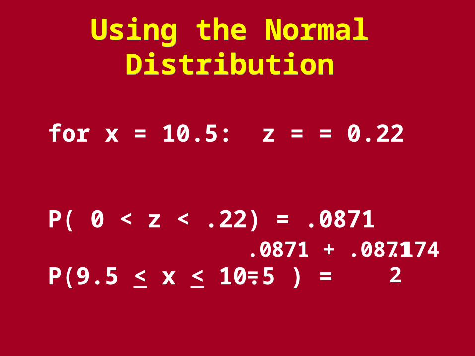
Using the Normal Distribution
Using the Normal Distribution
for x = 10.5: z = = 0.22
P( 0 < z < .22) = .0871
P(9.5 < x < 10.5 ) =.0871 + .0871 =.1742

Application of Normal Distribution
If 22% of all patients with high blood pressure have side effects from a certain medication, and 100 patients are treated,
find the probability that at least 30 of them will have side effects.
Using the Binomial Probability Formula we would need to compute:
P(30) + P(31) + ... + P(100) or 1 P( x < 29)
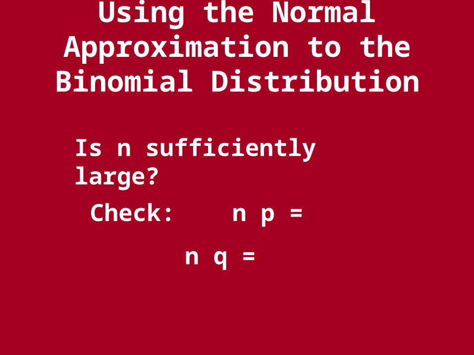
Using the Normal Approximation to the Binomial Distribution
Is n sufficiently large?
Check: n p =
n q =
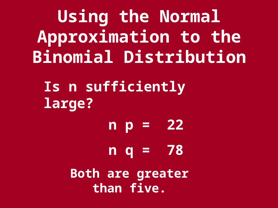
Using the Normal Approximation to the Binomial Distribution
Is n sufficiently large?
n p = 22
n q = 78
Both are greater than five.
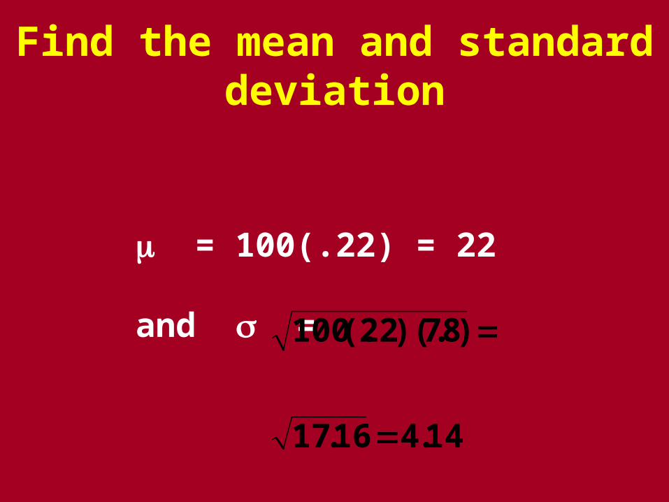
Find the mean and standard deviation
= 100(.22) = 22
and =
14.416.17
)78)(.22(.100
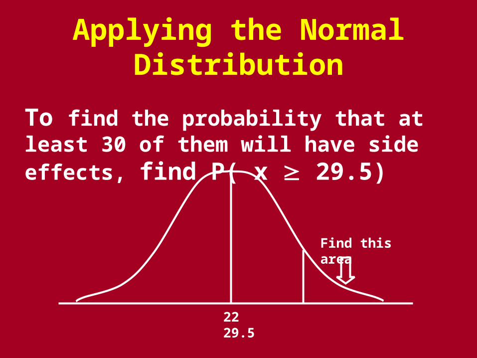
Applying the Normal Distribution
To find the probability that at least 30 of them will have side effects, find P( x 29.5)
22 29.5
Find this area
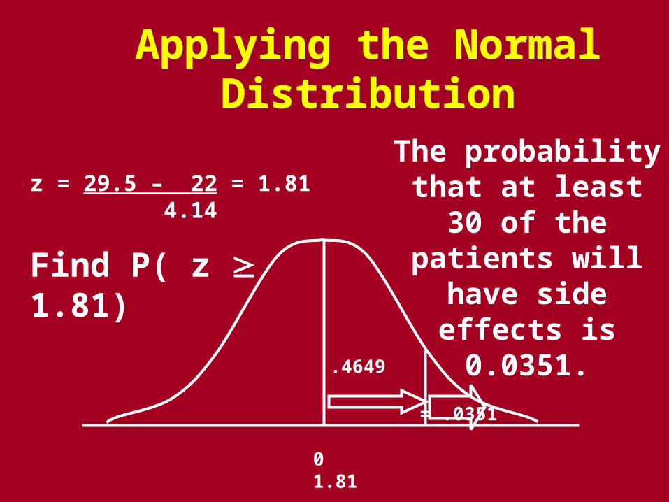
Applying the Normal Distribution
Applying the Normal Distribution
z = 29.5 – 22 = 1.81 4.14
Find P( z 1.81)
0 1.81
= .0351
.4649
The probability that at least 30 of the patients will have side effects
is 0.0351.
Reminders:
• Use the normal distribution to approximate the binomial only if both np and nq are greater than 5.
• Always use the continuity correction when approximating the binomial distribution.