Understanding Cable & Antenna AnalysisBy Stefan Pongratz

TABLE OF CONTENTS

1.0 Introduction 2

2.0 Frequency Domain Reflectrometry 2 3.0 Return Loss 3

4.0 Cable Loss 5

5.0 Cable Loss Effect on System Return Loss 5

6.0 Distance-To-Fault (DTF) 7

7.0 Fault Resolution, Display Resolution, and Max Distance 8

8.0 DTF Example 9

9.0 Interpreting DTF Measurements 9

10.0 Summary 11

2

1.0 IntroductionThe cable and antenna system plays a crucial role of the overall performance of a Base Station system. Degradations and failures in the antenna system may cause poor voice quality or dropped calls. From a carrier standpoint, this could eventually result in loss of revenue.

While a problematic base station can be replaced, a cable and antenna system is not so easy to replace. It is the role of the field technician to troubleshoot the cable and antenna system and ensure that the overall health of the communication system is performing as expected.

Field technicians today rely on portable cable and antenna analyzers to analyze, troubleshoot, characterize, and maintain the system. The purpose of this white paper is to cover the fundamentals of the key measurements of cable and antenna analysis: Return Loss, Cable Loss, and Distance-To-Fault (DTF).

2.0 Frequency Domain ReflectometryMost modern analyzers characterize the antenna system and use the Frequency Domain Reflectometry (FDR) technology. This technology uses RF frequencies to analyze the data, providing the ability to locate changes and degradations at the frequency of operation. Analyzing the data in the frequency domain enable users to find small degradations or changes in the system, and thus can prevent severe system failures. Another major benefit of analyzing the system using RF sweeps is that antennas are tested at their correct operating frequency and the signal will go through frequency selective devices such as filters, quarter-wave lightning arrestors, or duplexers that are common to cellular antenna systems.

The main advantage of using FDR-based technologies vs. Time Domain Reflectometry (TDR) is that the source energy in the operating band is much greater. This then results in better sensitivity and an improved likelihood of finding small problems before they become major

Sour ce’s Spect ral Densi ty

f1 f2

FDR

Less than 2% of TDR source energy is in the RF bands

3

3.0 Return Loss / Voltage Standing Wave Ratio (VSWR)The Return Loss and VSWR measurements are key measurements for anyone making cable and antenna measurements in the field. These measurements show the user the match of the system and if it conforms to system engineering specifications. If problems show up during this test, there is a very good likelihood that the system has problems that will affect the end user. A poorly matched antenna will reflect costly RF energy that will not be available for transmission and will instead end up in the transmitter. This extra energy returned to the transmitter will not only distort the signal, but it will also affect the efficiency of the transmitted power and the corresponding coverage area.

For instance, a 20 dB system Return Loss measurement is considered very efficient, as only 1% of the power is returned and 99% of the power is transmitted. If the Return Loss is 10 dB, 10% of the power is returned. While different systems have different acceptable return loss limits, 15 dB or better is a common system limit for a cable and antenna system.

RL: 20 d B 1 % pow er returned

RL: 10 d B 10 % pow er retu rn ed

While an antenna system could be faulty for any number of reasons, poorly installed connectors, dented/damaged coax cables, and defec-tive antennas tend to dominate the failure trends.

Return Loss and VSWR both display the match of the system but they show it in different ways. The Return Loss displays the ratio of reflected power to reference power in dB. The Return Loss view is usually pre-ferred because of the benefits with logarithmic displays; one of them being that it is easier to compare a small and large number on a loga-rithmic scale.

The Return Loss scale is normally set up from 0 to 60 dB with 0 being an open or a short and 60 dB would be close to a perfect match.

4

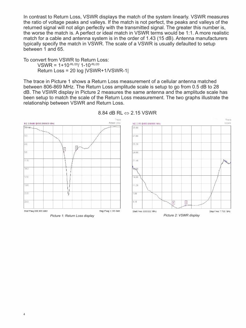
In contrast to Return Loss, VSWR displays the match of the system linearly. VSWR measures the ratio of voltage peaks and valleys. If the match is not perfect, the peaks and valleys of the returned signal will not align perfectly with the transmitted signal. The greater this number is, the worse the match is. A perfect or ideal match in VSWR terms would be 1:1. A more realistic match for a cable and antenna system is in the order of 1.43 (15 dB). Antenna manufacturers typically specify the match in VSWR. The scale of a VSWR is usually defaulted to setup between 1 and 65.

To convert from VSWR to Return Loss: VSWR = 1+10-RL/20/ 1-10-RL/20

Return Loss = 20 log |VSWR+1/VSWR-1|

The trace in Picture 1 shows a Return Loss measurement of a cellular antenna matched between 806-869 MHz. The Return Loss amplitude scale is setup to go from 0.5 dB to 28 dB. The VSWR display in Picture 2 measures the same antenna and the amplitude scale has been setup to match the scale of the Return Loss measurement. The two graphs illustrate the relationship between VSWR and Return Loss.

8.84 dB RL ⇔ 2.15 VSWR

Picture 2: VSWR displayPicture 1: Return Loss display

5

4.0 Cable LossAs the signal travels through the transmission path, some of the energy will be dissipated in the cable and the components. A Cable Loss measurement is usually made at the installation phase to ensure that the cable loss is within manufacturer’s specification.

The measurement can be made with a portable vector/scalar network analyzer or a power meter. Cable loss can be measured using the Return Loss measurement available in the cable and antenna analyzer. By placing a short at the end of the cable, the signal is reflected back and the energy lost in the cable can be computed. Equipment manufacturers suggest to get the average cable loss of the swept frequency range, add the peak of the trace to the valley of the trace and divide by two in Cable Loss mode or divide by four in Return Loss mode (to account for the signal traveling back and forth).

Most portable cable and antenna analyzers today are equipped with a Cable Loss mode that displays the average cable loss of the swept frequency range. This is usually the preferred method since it eliminates the need for any math. The graph in Picture 3 below shows a cable loss measurement of a cable between 1850 and 1990 MHz. The markers at the peak and valley can be used to compute the average. This particular handheld instrument computes the average cable loss for the user as can be seen in the left part of the display.

Increasing the RF frequency and the length of the cable will increase the insertion loss. Cables with larger diameter have less insertion loss and better power handling capabilities than cables with smaller diameter.

5.0 Cable Loss Effect on System Return Loss The insertion loss of the cable needs to be taken into consideration when making system return loss measurements. Picture 4 illustrates how cable loss changes the perceived antenna performance. The antenna itself has a return loss of 15 dB but the 5 dB insertion loss improves the perceived system return loss by 10 dB (5 dB *2). Even though this is something system designers take into consideration when setting up the specifications of the site, it is important to be aware of the effects the insertion loss and cable return loss can have on the overall system return loss. A very good system return loss may not necessarily be the result of an excellent antenna; it could be a faulty cable with too much insertion loss and an antenna out of specification. This would result in a larger than expected signal drop and once the signal reaches the antenna, a great portion of the signal is now reflected since the match is worse than expected. The end result is that the transmitted signal is lower than needed and the overall coverage area is now affected. In other words, if your system return loss is too good, it is not always a good thing.

Picture 3: Cable Loss Measurement

6

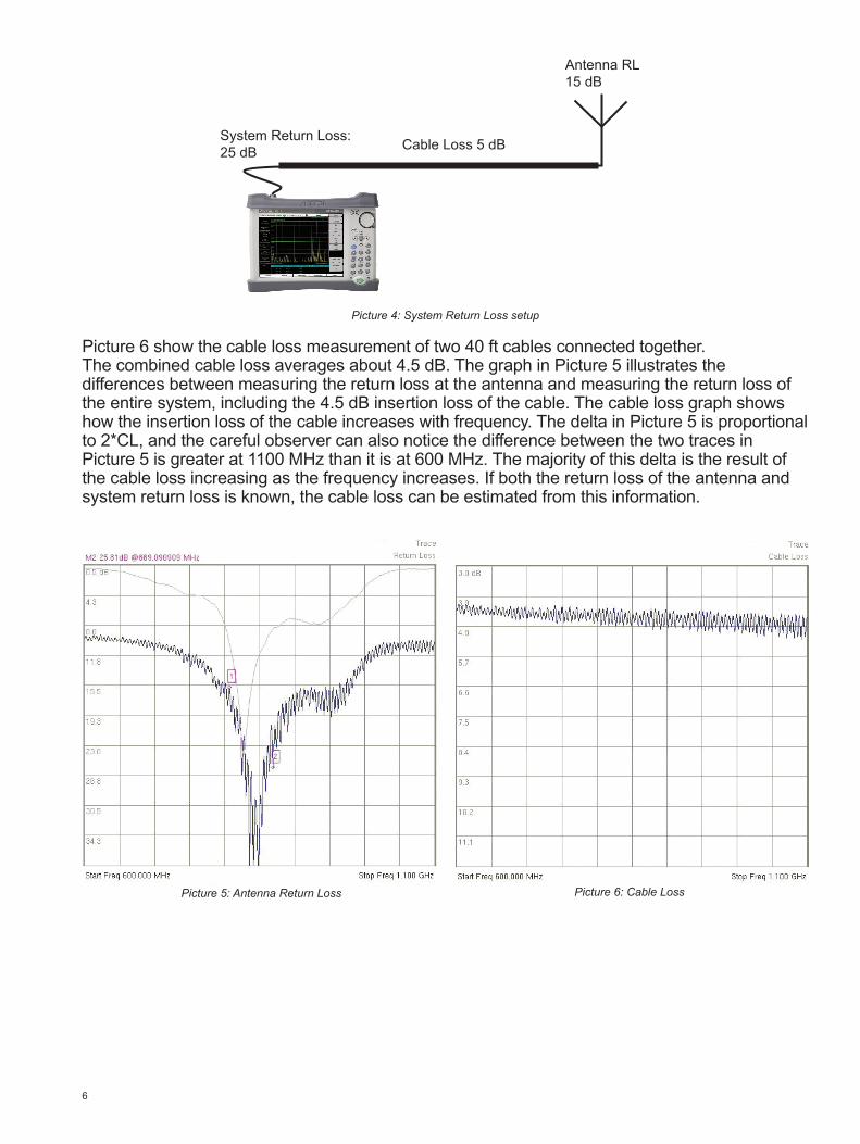
Picture 6 show the cable loss measurement of two 40 ft cables connected together. The combined cable loss averages about 4.5 dB. The graph in Picture 5 illustrates the differences between measuring the return loss at the antenna and measuring the return loss of the entire system, including the 4.5 dB insertion loss of the cable. The cable loss graph shows how the insertion loss of the cable increases with frequency. The delta in Picture 5 is proportional to 2*CL, and the careful observer can also notice the difference between the two traces in Picture 5 is greater at 1100 MHz than it is at 600 MHz. The majority of this delta is the result of the cable loss increasing as the frequency increases. If both the return loss of the antenna and system return loss is known, the cable loss can be estimated from this information.

System Return Loss:25 dB Cable Loss 5 dB

Antenna RL15 dB

Picture 4: System Return Loss setup

Picture 6: Cable LossPicture 5: Antenna Return Loss

7

6.0 Distance-To-Fault (DTF)Return Loss / VSWR measurement characterizes the performance of the overall system. If either of these is failing, the DTF measurement can be used to troubleshoot the system and locate the exact location of a fault. It is important to understand that the DTF measurement is strictly a troubleshooting tool, and best used to compare relative data and monitor changes over time with the main purpose of locating faults and measuring the length of the cable. Using the DTF absolute amplitude values derived from the DTF data as a replacement for return loss or as a pass/fail indicator is not recommended. There are so many variables that affect the DTF readings, including propagation velocity variation, insertion loss inaccuracies of the complete system, stray signals, temperature variations, and mathematical limitations, it is very challenging for system engineers to come up with numbers that take all of this into consideration. Used correctly, the DTF measurement is by far the best method for troubleshooting cable and antenna problems.

The DTF measurement is based on the same information as a Return Loss or Cable Loss measurement. The DTF measurement sweeps the cable in the frequency domain and then, with the help of the Inverse Fast Fourier Transform (IFFT), the data can be converted from the frequency domain to the time domain. In other words, if you forgot to do a DTF measurement but made a Return Loss measurement and still have access to the magnitude and phase data of the 1-port measurement, you don’t have to worry because the magnitude and phase data can be used to create a DTF plot in software.

The dielectric material in the cable affects the propagation velocity that affects the velocity of the signal traveling through the cable. The accuracy of the propagation velocity (vp) value will determine the accuracy of the location of the discontinuity. A ± 5% error in the vp value will affect the distance accuracy accordingly, and the end of the 80 ft cable could show up anywhere between 76 and 84 ft . Even if the vp value is copied out of the manufacturer’s datasheet, there could still be some discrepancies between the interpreted and actual distance discontinuities. This is a result of adding all the components in the system. Common base station systems can include a main feed line, feed line jumper, adapters, and top jumpers. Even though the main feed line contributes with the largest amount, the velocity of the signal through the other parts of the system could be different.

The accuracy of the amplitude values are usually of less importance because DTF should be used to troubleshoot a system and find problems. So whether a connector is at 30 dB or 35 dB may not be as interesting as if the connector was at 35 dB one year ago and now it is at 30 dB. While the propagation velocity value remains fairly constant over the entire frequency range, the insertion loss of the cable does not and this also affects the amplitude accuracy.

Most handheld instruments available today have built-in tables that include propagation velocity values and cable insertion loss values for different frequencies of the most commonly used cables. This simplifies the task for the field technician as they can locate the cable type, and obtain the correct vp and cable loss values.

The table below shows different cable loss levels for two commonly used cables. Cable Prop Velocity 1000 MHz 2500 MHz

Andrew LDF4-50A 0.88 0.073 dB/m 0.120 dB/mAndrew HJ4.5-50 0.92 0.054 dB/m 0.089 dB/m

8

7.0 Fault Resolution, Display Resolution, and Max DistanceThe term resolution can be confusing and the definitions can vary. For DTF, it is important to understand the difference between fault resolution and display resolution because the meanings are different.

Fault resolution is the system’s ability to separate two closely spaced signals. Two discontinuities located 0.5 ft apart from each other will not be identified in a DTF measurement if the fault resolution is 2 ft. Because DTF is swept in the frequency domain, the frequency range affects the fault resolution. A wider frequency ranges means better fault resolution and shorter max distance. Similarly, a narrower frequency range leads to wider fault resolution and greater maximum horizontal distance. The only way to improve the fault resolution is to increase the frequency range.

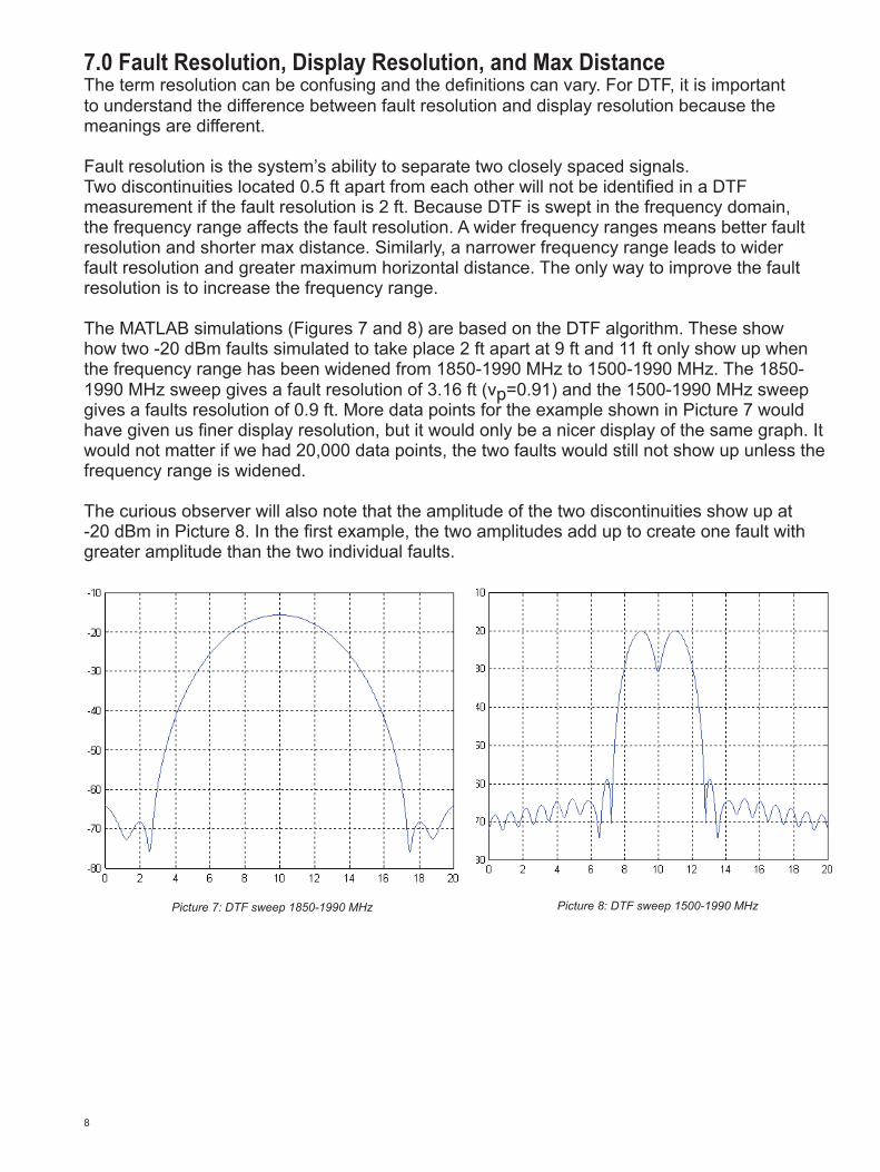
The MATLAB simulations (Figures 7 and 8) are based on the DTF algorithm. These show how two -20 dBm faults simulated to take place 2 ft apart at 9 ft and 11 ft only show up when the frequency range has been widened from 1850-1990 MHz to 1500-1990 MHz. The 1850-1990 MHz sweep gives a fault resolution of 3.16 ft (vp=0.91) and the 1500-1990 MHz sweep gives a faults resolution of 0.9 ft. More data points for the example shown in Picture 7 would have given us finer display resolution, but it would only be a nicer display of the same graph. It would not matter if we had 20,000 data points, the two faults would still not show up unless the frequency range is widened.

The curious observer will also note that the amplitude of the two discontinuities show up at -20 dBm in Picture 8. In the first example, the two amplitudes add up to create one fault with greater amplitude than the two individual faults.

Picture 7: DTF sweep 1850-1990 MHz Picture 8: DTF sweep 1500-1990 MHz

9

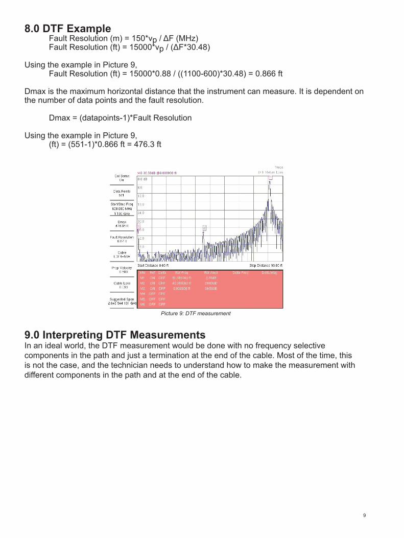
8.0 DTF Example Fault Resolution (m) = 150*vp / ΔF (MHz) Fault Resolution (ft) = 15000*vp / (ΔF*30.48)

Using the example in Picture 9, Fault Resolution (ft) = 15000*0.88 / ((1100-600)*30.48) = 0.866 ft

Dmax is the maximum horizontal distance that the instrument can measure. It is dependent on the number of data points and the fault resolution.

Dmax = (datapoints-1)*Fault Resolution

Using the example in Picture 9, (ft) = (551-1)*0.866 ft = 476.3 ft

9.0 Interpreting DTF MeasurementsIn an ideal world, the DTF measurement would be done with no frequency selective components in the path and just a termination at the end of the cable. Most of the time, this is not the case, and the technician needs to understand how to make the measurement with different components in the path and at the end of the cable.

Picture 9: DTF measurement

10

Picture 10 and 11 below show graphs of the DTF measurements of the same instrument setup. The two 40 ft LDF4-50A cables are connected together with an open at the end of the cable in Picture 10 and a PCS antenna connected to the end of the cable in Picture 11. The only difference between the two graphs is the amplitude level of the peak showing the end of the cable.

Picture 12 shows a kink in the cable just 7 ft before the antenna.

Picture 10: DTF Open Picture 11: DTF PCS antenna

Picture 12: DTF PCS antenna with fault

11

Picture 14 shows how the electrical length of the TMA in Picture 13 affects the distance measurement of the system. The graph in Picture 13 shows a transmission measurement of a 2-port dual duplex LNA. Picture 14 shows the DTF measurement of this system swept with the TMA in the path. The end connection shows up at 106 ft because the TMA was swept over both the uplink and downlink bands of the TMA. The end of the same system without the TMA in the path shows up at 83 ft (Picture 14).

10.0 SummaryThe cable and antenna system plays an important role in the overall performance of the cell site. Small changes in the antenna system can affect the signal, coverage area and eventually cause dropped calls. Using portable cable and antenna analyzers to characterize communication systems can simplify maintenance and overall performance significantly. The return loss/VSWR measurements are used to characterize the system. If the match is outside the system specification, the DTF measurement can be used to troubleshoot problems, locate faults, and monitor changes over time.

Picture 13: 2-port measurement of TMA Picture 14: DTF with TMA in path

11410-00427, Rev. F Printed in United States 2017-10 ©2017 Anritsu Company. All Rights Reserved.

® Anritsu All trademarks are registered trademarks of their respective companies. Data subject to change without notice. For the most recent specifications visit: www.us.anritsu.com

Anritsu utilizes recycled paper and environmentally conscious inks and toner.

• United States Anritsu Company1155 East Collins Boulevard, Suite 100, Richardson, TX, 75081 U.S.A. Toll Free: 1-800-267-4878 Phone: +1-972-644-1777 Fax: +1-972-671-1877• Canada Anritsu Electronics Ltd.700 Silver Seven Road, Suite 120, Kanata, Ontario K2V 1C3, Canada Phone: +1-613-591-2003 Fax: +1-613-591-1006

• Brazil Anritsu Electrônica Ltda.Praça Amadeu Amaral, 27 - 1 Andar 01327-010 - Bela Vista - São Paulo - SP - Brazil Phone: +55-11-3283-2511 Fax: +55-11-3288-6940

• Mexico Anritsu Company, S.A. de C.V.Av. Ejército Nacional No. 579 Piso 9, Col. Granada 11520 México, D.F., México Phone: +52-55-1101-2370 Fax: +52-55-5254-3147

• United Kingdom Anritsu EMEA Ltd.200 Capability Green, Luton, Bedfordshire LU1 3LU, U.K. Phone: +44-1582-433280 Fax: +44-1582-731303

• France Anritsu S.A.12 avenue du Québec, Batiment Iris 1-Silic 612, 91140 Villebon-sur-Yvette, France Phone: +33-1-60-92-15-50 Fax: +33-1-64-46-10-65

• Germany Anritsu GmbHNemetschek Haus, Konrad-Zuse-Platz 1 81829 München, Germany Phone: +49-89-442308-0 Fax: +49-89-442308-55

• Italy Anritsu S.r.l.Via Elio Vittorini 129, 00144 Roma Italy Phone: +39-06-509-9711 Fax: +39-06-502-2425

• Sweden Anritsu ABKistagången 20B, 164 40 KISTA, Sweden Phone: +46-8-534-707-00 Fax: +46-8-534-707-30

• Finland Anritsu ABTeknobulevardi 3-5, FI-01530 Vantaa, Finland Phone: +358-20-741-8100 Fax: +358-20-741-8111

• Denmark Anritsu A/SKay Fiskers Plads 9, 2300 Copenhagen S, Denmark Phone: +45-7211-2200 Fax: +45-7211-2210• Russia Anritsu EMEA Ltd.Representation Office in RussiaTverskaya str. 16/2, bld. 1, 7th floor. Russia, 125009, Moscow Phone: +7-495-363-1694 Fax: +7-495-935-8962

• United Arab EmiratesAnritsu EMEA Ltd. Dubai Liaison OfficeP O Box 500413 - Dubai Internet City Al Thuraya Building, Tower 1, Suite 701, 7th Floor Dubai, United Arab Emirates Phone: +971-4-3670352 Fax: +971-4-3688460

• Singapore Anritsu Pte. Ltd.11 Chang Charn Road, #04-01, Shriro House Singapore 159640 Phone: +65-6282-2400 Fax: +65-6282-2533

• India Anritsu India Pvt Ltd.2nd & 3rd Floor, #837/1, Binnamangla 1st Stage, Indiranagar, 100ft Road, Bangalore - 560038, India Phone: +91-80-4058-1300 Fax: +91-80-4058-1301• P. R. China (Shanghai) Anritsu (China) Co., Ltd.27th Floor, Tower A, New Caohejing International Business Center No. 391 Gui Ping Road Shanghai, Xu Hui Di District, Shanghai 200233, P.R. China Phone: +86-21-6237-0898 Fax: +86-21-6237-0899

• P. R. China (Hong Kong) Anritsu Company Ltd.Unit 1006-7, 10/F., Greenfield Tower, Concordia Plaza, No. 1 Science Museum Road, Tsim Sha Tsui East, Kowloon, Hong Kong, P. R. China Phone: +852-2301-4980 Fax: +852-2301-3545

• Japan Anritsu Corporation8-5, Tamura-cho, Atsugi-shi, Kanagawa, 243-0016 JapanPhone: +81-46-296-1221 Fax: +81-46-296-1238

• Korea Anritsu Corporation, Ltd.5FL, 235 Pangyoyeok-ro, Bundang-gu, Seongnam-si, Gyeonggi-do, 463-400 Korea Phone: +82-31-696-7750 Fax: +82-31-696-7751

• Australia Anritsu Pty Ltd.Unit 21/270 Ferntree Gully Road, Notting Hill, Victoria 3168, Australia Phone: +61-3-9558-8177 Fax: +61-3-9558-8255

• Taiwan Anritsu Company Inc.7F, No. 316, Sec. 1, Neihu Rd., Taipei 114, Taiwan Phone: +886-2-8751-1816 Fax: +886-2-8751-1817