Jan/Feb 2001 37

Old-fashioned microwave engineering.

By Paul Wade, W1GHZ

161 Center RdShirley, MA 01414w1ghz@arrl.net

Understanding CircularWaveguide—Experimentally

1Notes appear on page 48.

Waveguide is an excellent mi-crowave transmission line,with low loss and predictable

performance, usable at any frequencyby choosing the proper dimensions. Themost common type of commercial wave-guide is precision rectangular tubing,which is only affordable on the surplusmarket. Elliptical waveguide is alsoused commercially for microwavetransmission line. Many microwavestructures, particularly antennas, havea round cross section and are bettersuited to circular (cylindrical) wave-guide. Unfortunately, commercial cir-cular waveguide is rare and unlikely to

be found surplus. As luck would have it,ordinary copper water pipe works justfine and is universally available at lowcost. In particular, 3/4-inch copper pipeis perfect for 10 GHz.

Most microwave design today is donewith the aid of computers. However,only a few programs handle electro-magnetics with the capabilities re-quired for circular waveguide, and theirprices are somewhere between a fancycar and a new house. Solving the prob-lems without good software involvessome difficult math, and the solution isprobably only approximate. The re-maining alternative is old-fashionedempirical microwave engineering.

The ham’s favorite design technique,reverse engineering (copying some-thing that works!) is made difficult bythe lack of commercial circular-

waveguide examples. Reference bookshave extensive information on rectan-gular waveguide but very little infor-mation on circular waveguide. The pio-neering work on waveguides was doneby George Southworth before WorldWar II, but I only recently located acopy of his book.1 I was afraid that Ihad duplicated some of his work, butthat’s a good way to learn. On firstreading, it appears that he did a lot ofwork on waveguide fundamentals, butvery little on waveguide-to-coax tran-sitions, probably because good coaxialcable and connectors were not avail-able prior to the wartime development.

Circular WaveguideWe all know that electromagnetic

Reprinted with permission; copyright ARRL.

38 Jan/Feb 2001

waves travel through space—that’swhat radio is all about. They can alsotravel inside a hollow pipe of any shape;if the dimensions are right, the pipemakes a very low-loss transmissionline, much better than any coaxialcable. In order for the waves to travelwith low loss, the pipe dimensions mustbe large enough for the lowest-orderwaveguide mode, the TE11 mode, topropagate. In circular waveguide, thecutoff wavelength for this mode is1.706×D (diameter) so the minimumwaveguide diameter is 1/1.706, or0.59 λ. The diameter of the copper wa-ter pipe I used is nominally 3/4-inch,type M, which has a larger inner diam-eter than other types. The typical innerdiameter is 0.81 inches, but that mayvary slightly because this is not preci-sion tubing. Thus, the cutoff wave-length is 1.38 inches, so the minimumfrequency is 8.55 GHz. Clearly, 10 GHzis comfortably above the minimum.

Moving in the other direction, alarge waveguide diameter would per-mit additional higher-order wave-guide modes to propagate. While theadditional modes also propagate withlow loss, they often arrive at the farend with different phase, so that theyinterfere with the TE11 wave and weare unable to extract them withoutlosses. The next mode, TM01, needs aminimum diameter of 0.76 λ to propa-gate, setting the maximum operatingfrequency without any additionalmodes. For the 3/4-inch pipe, this up-per frequency limit is 11.08 GHz, butit isn’t a hard limit like the lower cut-off frequency. At higher frequencies,the waveguide still propagates en-ergy, it’s just difficult to predictablycouple that energy efficiently.

Thus, a hollow round pipe is an ex-cellent waveguide for wavelengths be-tween 0.59 and 0.76 times the insidediameter. Standard USA 3/4-inch cop-per water pipe, type M, has an innerdiameter of 0.70 λ at 10.368 GHz, so itis ideal for 10-GHz operation. It isreadily available in almost any hard-ware store at a cost much lower thanthat of coaxial cable suitable for VHFuse. Copper water pipe does come inother versions, but type M is preferablesince it has the largest inner diameter.

MeasurementOur design style is “old-fashioned

empirical microwave engineering.”“Empirical” is a fancy word for “cut andtry,” but it is only engineering if wemake measurements, record data andtry to understand the results.

The most important measurement we

need is impedance in the waveguide.Today, impedance measurements aremade using a network analyzer, prefer-ably one that is automated, with com-puter control and error corrections.There aren’t any waveguide networkanalyzers; they are all based on coaxialtransmission lines. For the most popu-lar standard sizes of rectangular wave-guide, good coaxial transitions and cali-bration kits are available to allow net-work-analyzer measurements, with thecomputer correcting errors caused bythe transitions. Of course, none of thisis available for circular waveguide—ifwe had a quality coax transition to copy,we’d be one giant step closer to usingcircular waveguide.

Before network analyzers, micro-wave impedance measurements weremade using a slotted line. A narrowlongitudinal slot in the outer conduc-tor of a coaxial line does not interruptany current flow in the line, so it has noeffect. A small probe may be insertedin the slot to measure the voltage in theline, and moved to measure the voltageat other points along the line. If the lineis mismatched, the voltage varies in apattern referred to as a standing wave.Normally, we measure the ratio be-tween the minimum and maximumvoltages of the standing wave and callit the standing wave ratio, or SWR.Using a slotted line is becoming a lostart, but the technique is covered prettywell in a recent book by Pozar.2

In waveguide, a slot will have no ef-fect if it does not interrupt any current.In rectangular waveguide, this locationis easy to find. It’s in the center ofthe broad wall. In circular waveguide,there is no obvious orientation; we must

orient the guide so that the E-field issymmetrical around the slot and theprobe is parallel to the E-field.

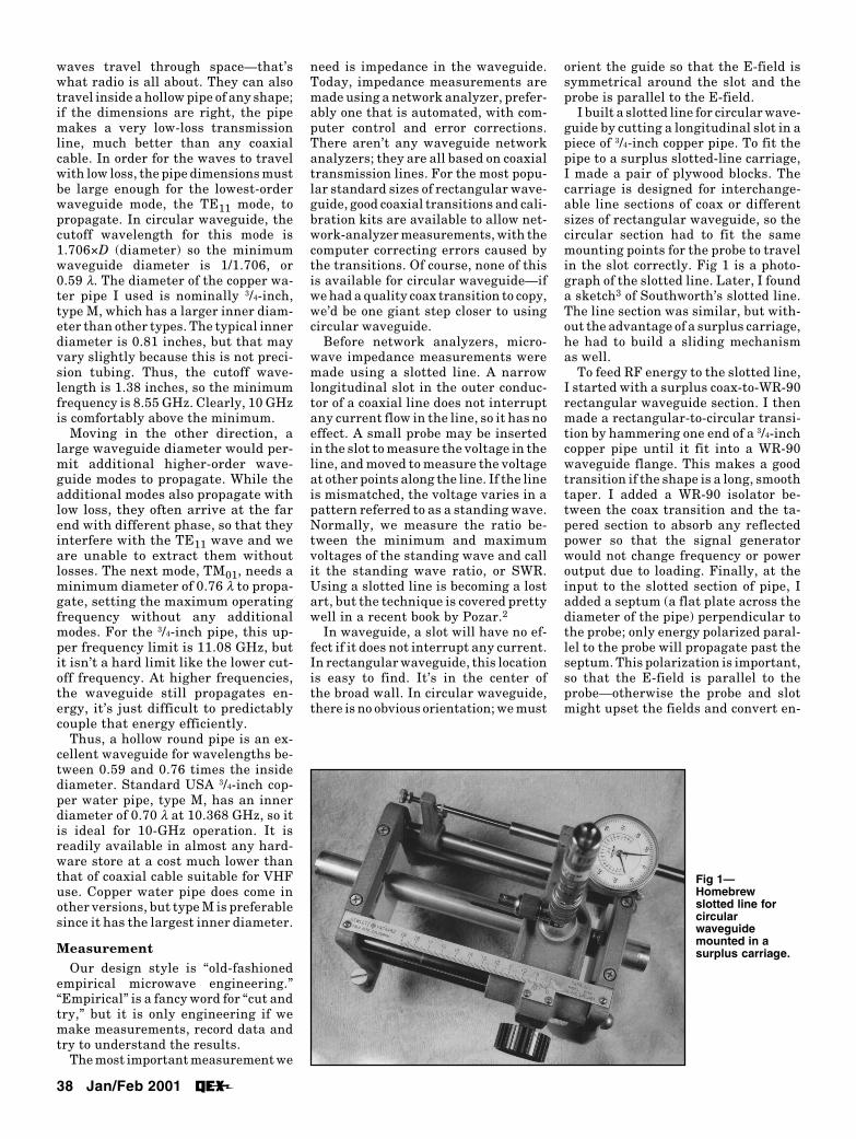
I built a slotted line for circular wave-guide by cutting a longitudinal slot in apiece of 3/4-inch copper pipe. To fit thepipe to a surplus slotted-line carriage,I made a pair of plywood blocks. Thecarriage is designed for interchange-able line sections of coax or differentsizes of rectangular waveguide, so thecircular section had to fit the samemounting points for the probe to travelin the slot correctly. Fig 1 is a photo-graph of the slotted line. Later, I founda sketch3 of Southworth’s slotted line.The line section was similar, but with-out the advantage of a surplus carriage,he had to build a sliding mechanismas well.

To feed RF energy to the slotted line,I started with a surplus coax-to-WR-90rectangular waveguide section. I thenmade a rectangular-to-circular transi-tion by hammering one end of a 3/4-inchcopper pipe until it fit into a WR-90waveguide flange. This makes a goodtransition if the shape is a long, smoothtaper. I added a WR-90 isolator be-tween the coax transition and the ta-pered section to absorb any reflectedpower so that the signal generatorwould not change frequency or poweroutput due to loading. Finally, at theinput to the slotted section of pipe, Iadded a septum (a flat plate across thediameter of the pipe) perpendicular tothe probe; only energy polarized paral-lel to the probe will propagate past theseptum. This polarization is important,so that the E-field is parallel to theprobe—otherwise the probe and slotmight upset the fields and convert en-

Fig 1—Homebrewslotted line forcircularwaveguidemounted in asurplus carriage.

Jan/Feb 2001 39

ergy to unwanted waveguide modes,with unpredictable results and strangemeasurements.

The voltage in the slotted line issampled by the probe inserted throughthe slot; if the probe is inserted too far,it will affect the fields in the waveguideand produce erroneous readings. Onthe other hand, a deeper probe producesmore output voltage, so less RF poweris necessary for the measurement. Theproper probe depth is found experimen-tally, by increasing the depth until themeasured SWR starts to change, thenbacking off.

The probe assembly shown in Fig 1contains a diode detector with a tuningmechanism; when it is adjusted forresonance, much more detected voltageis available. The output from the detec-tor goes to a standing-wave meter suchas an HP415; other manufacturersmade similar instruments. The meteris an ac voltmeter tuned to 1 kHz, sothe RF source must be AM modulatedat 1 kHz; most signal generators havethis capability.

Once the slotted line was working, Iquickly discovered two things:

1. The wavelength at 10 GHz isnearly twice as long in 3/4-inch wave-guide as it is in free space.

2. This means that the probe musttravel near the end of the slot to mea-sure a full wavelength.

As the probe approached the ends ofthe slot, I could see that there was aneffect. A well-matched horn antennahad a low indicated SWR with the probenear the center of the slot, but a higherindication when it was near the ends.Since commercial rectangular-wave-guide slotted sections taper the end ofthe slot to a point, I used a tapered fileto trim the ends of the slot to smooththe response.

Wavelength in the waveguide ismeasured by shorting the end of thewaveguide with a flat plate; this pro-duces a standing-wave pattern with anull every λ/2 from the short. I knewthat guide wavelength, λg, would belonger than the wavelength in freespace, λ0, (phase velocity is greaterthan the speed of light), but hadn’trealized how much longer. Fig 2 showsλg versus frequency; as the cutoff fre-quency is approached, λg increasesdramatically, while λ0 increases lin-early with decreasing frequency.

Impedance is measured and calcu-lated graphically by plotting SWR andphase on a Smith chart. Phase is mea-sured by the location of the standing-wave minimum voltage on the slottedline. The distance between two stand-

ing-wave minimums is λg/2. With ashort circuit on the end of the slottedline, we can locate two voltage nulls onthe line to provide the reference pointsfor our measured location. A classicSmith chart has a wavelength scalearound the perimeter that is used toplot phase; the circumference of thechart equals λ/2.

On a Smith chart, the impedance isnormalized to the characteristic imped-ance of the transmission line. Commoncoaxial lines have characteristic imped-ances near 50 Ω. For waveguide, we usewave impedance rather than character-istic impedance. The wave impedancefor TE modes in circular waveguide iscalculated as:

Z0 = Zfs

λg

λ0

(Eq 1)

where Zfs is the impedance of freespace, 377 Ω. From Fig 2, the guidewavelength, λg is longer than the free-space wavelength λ0, so our circularwaveguide impedance is greater than377 Ω. Unlike coaxial transmissionlines, the impedance varies with fre-quency. At 10.368 GHz, Z0 is about650 Ω; however, it is about 1130 Ω at9 GHz and 580 Ω at 11.2 GHz. For ourpurposes, the exact impedance doesnot matter, as long as we can match itempirically and achieve a low SWR. Infact, I did not calculate Z0 until afterI had completed all the experimentalwork described here.

For phase measurements, the slottedline includes a vernier scale to measuredistance traveled; the scale is quiteaccurate if used carefully. However,once I realized that many slotted-line

Fig 2—Wavelength does not vary linearly in 3/4-inch circular waveguide.

Fig 3—Construction of a 3/4-inch pipe waveguide transition.

40 Jan/Feb 2001

measurements would be required, Iadded a dial indicator (shown in Fig 1)to the slotted line. The dial indicator,together with a dial caliper to measureprobe dimensions and backshort (I’llexplain this term shortly) distances,speeds up measurements significantly.Unfortunately, inexpensive dial cali-pers and indicators read in inches only,rather than the metric units preferredfor microwave work, so we will stick toinches. Anyway, it would be silly to re-fer to “3/4-inch pipe” in metric units.

Finally, we need a matched load.K2RIW reports carving a tapered pointon a broomstick to make a load for cir-cular waveguide, but a horn antennawith a long taper is known to provide adecent match. Therefore, I made asimple conical horn from copper flash-ing. The measured SWR is about 1.14:1.

Coaxial TransitionOur ultimate goal is to make better

antennas using circular waveguide, butthe antennas must connect to equip-ment that uses coaxial cable for inter-connections. I had already built severalfeed antennas for dishes that I wantedto test, but first I needed a good repro-ducible coax transition to connect them.The simplest coax transition extendsthe center conductor of the coax as aradial probe in the waveguide, as shownin Fig 3. The end of the waveguide be-hind the probe ends in a short circuitreferred to as a backshort.

My previous attempts at buildingtransitions from coax to circular wave-guide were not always successful. Anumber of designs have been publishedfor transitions at lower frequencies, butwith widely varying dimensions. Theones I have tried were not always wellmatched, and some were very critical.On closer examination, some of themare feeding mismatched antennas (suchas “coffee can” feeds or open circularwaveguides with typical SWRs of 2:1),so they are probably adjusted to a spe-

Fig 5—SWR versus backshort distance (in λλλλλg) for a probe diameter of 0.040 inches.

cific mismatch, rather than providing amatched transition.

On the other hand, coax transitionsto rectangular waveguide have beenmore successful, probably becausemany of them start with dimensions ofcommercial transitions. I have ad-justed some by making measurementswith a rectangular-waveguide slottedline. The measurements suggest thatthe three variable dimensions in awaveguide transition (shown in Fig 3)all interact. There are combinations ofprobe diameter, probe length and dis-tance to the backshort that transformthe impedance of the waveguide to adesired coax impedance, usually 50 ý.A textbook I consulted long ago sug-gested that there is an optimum probelength and backshort distance for eachdesired impedance, but the induc-tance of the probe must be compen-sated by changes in the length andbackshort distance. Since the induc-tance is a function of probe diameter,the calculations only provide a roughapproximation. Previous experimentsat lower frequencies showed that theapproximation was not very good.

Since calculations seemed inad-equate, experimentation seemed like agood alternative. I built a fully adjust-able coax transition, shown in Fig 4. Ahexagonal plumbing fitting providesflat sides for an SMA panel-mount con-nector, so the probe length and diam-eter can be changed quickly. The con-nector is held by two screws and theTeflon dielectric extends through thepipe wall so that the probe starts at the

inside wall of the waveguide, a repro-ducible position. A sliding backshortprovides a full adjustment range. Atlow frequencies, sliding finger stock isused to provide an adjustable short-circuit, but the fingers are too long toprovide a good short at 10 GHz. The al-ternative, shown in Fig 4, is steppedquarter-wave sections: the first sectionis a sliding fit in the pipe, which pro-vides a very low impedance. It isfollowed by a small-diameter high-impedance section, then another low-impedance section. The large sectionshave such low impedances that itdoesn’t really matter if they make con-tact; the result looks like a short circuitin the waveguide.

My strategy was to make some mea-surements with different probe diam-eters and find a good combination ofdimensions for each diameter. I thenplanned to make some bandwidthmeasurements to see which combina-tion was least critical, so it could beeasily reproduced and scaled to otherfrequencies.

To choose a range of probe diameters,I looked at published designs. Low-fre-quency designs, for instance 1296 MHz,often use a thin probe of #14 AWG wire.At 10 GHz, this scales to perhaps 0.012inches, which isn’t very substantial.Published designs for higher frequen-cies use probes as large as 0.093 inches,which scales to about a 3/4-inch diam-eter at 1296 MHz. This wide range ledme to try a range of diameters, from0.010 to 0.062 inches, at 10 GHz.

For each probe diameter, I measured

Fig 4—Adjustable circular waveguide-to-coax transition with a sliding short circuit.

Jan/Feb 2001 41

Fig 7—The SWR data of Fig 5 with some of the worst candidatesremoved.

Fig 6—The SWR data of Fig 5 plotted on a Smith chart.

the waveguide impedance with theSMA connector terminated in a good50-Ω termination. A low SWR in thewaveguide is a good transition. I madethe impedance measurement with thebackshort distance moving in λ/8 incre-ments, starting with long probe lengthsthat I trimmed in small increments.

The plan was simple: plot this data,spot a trend and zero in on optimumcombinations. The first plot was SWRonly, shown in Fig 5. This is what wewould be able to measure with a net-work analyzer or a directional coupler.Perhaps you can spot a trend in Fig 5,but I only found it confusing!

So much for simple plans, it wastime for the Smith chart. In my previ-ous work with rectangular waveguide,plotting a few points by hand was suf-ficient to understand what was goingon. However, I now had dozens of datapoints and no clear idea of which ofthem was worth plotting. I down-loaded some Smith-chart routinesfrom the Internet, picked a good oneand added some code to plot my datain smooth curves on the Smith chart.

The confusing SWR data in Fig 5 isplotted on the Smith chart in Fig 6,with the addition of phase to makeeach data point a complex impedance.The data shown is for a probe diameterof 0.040 inches. Each solid curve plotsa constant probe length with differentbackshort distances. The points arestill well scattered, but one curve, forthe shortest probe length of 0.109 λ,circles around the center of the Smithchart while the other curves are all onthe left side of center. Thus, we mightsuspect that the optimum probelength may be somewhere between theshortest length and the next longest.

Fig 7 removes the curves for some ofthe longer probe lengths to concen-trate on the ones that bracket thebull’s-eye, the center of the chart. Thedashed curves intersecting them areplots of constant backshort distancewith varying probe length—what youwould see if you soldered together atransition and could only trim theprobe length. It’s clear that neither ofthese adjustments alone will producea good transition unless the other is

just right, but one of the dashed linesgoes right through the center. Theoptimum backshort distance should bevery close to 0.25 λg, or 0.250 guidewavelengths. The points I measuredbracket the bull’s-eye, so based onthose values I tried to estimate a probelength that would land dead center.

Fig 8 is a Smith chart showing thethree curves from Fig 7 plus one addi-tional curve, the dashed line, for a probelength that was my estimate of opti-mum. The best point on this curve hasa SWR of 1.05, a decent match. Thereisn’t much point in trying to do better,since neither the slotted line nor the50-Ω termination on the SMA connec-tor is perfect—each of the measure-ments has some error and uncertainty.

The horizontal centerline on theSmith chart is the resistive axis; pointson the line are purely resistive. Imped-ances greater than Z0, the wave imped-ance, are to the right of the centerpoint, while lesser impedances are tothe left. Points off the centerline havereactive components—inductance isabove the centerline, capacitance be-

42 Jan/Feb 2001

low. So we can see some trends on theseSmith charts: Longer probes producelower resistances, while longer back-short distances move the reactancefrom inductive to capacitive. While itis clear from Fig 7 that these aren’tstraight lines, we can use these trendsto “zero in” once we are close.

Returning to Fig 5, we can start tounderstand the curves. The threeshortest lengths are the curves inFig 7 that bracket the bull’s-eye, butthe SWR plot doesn’t really make thisclear. The other curves, for longerprobes, all have a sharp minimumsomewhere near a backshort distanceof 0.375 λg; this looks suspiciously likea resonance. Since it is much easier toshorten a probe than to make it longer,I start with an overly long one andtrim until it seems to be too short.Therefore, more data is taken withlong probes than short ones.

On a Smith chart, we can see combi-nations of probe length and backshortdistance that bracket the desiredmatch at the center of the chart, thenestimate the ideal combination from

Fig 8—The SWR curves of Fig 7 with a new dashed linerepresenting the estimated optimum solution.

Fig 9—SWR curves for a 3/4-inch water pipe circular waveguide-to-coax transition. Probe diameter=0.050 inches.

these data points. I did this for a rangeof probe diameters from 0.010 to 0.062inches. Fig 9 is the Smith chart for aprobe diameter of 0.050 inches, thediameter of the center pin of an SMAjack. For this diameter, I again foundthree curves that bracket the bull’s-eye, then estimated the best lengthand measured it for the dashed curve.The lighter dotted lines are plots forconstant backshort distance. Fig 10shows the same set of curves for thelargest probe diameter, 0.062 inches,but without the lighter dotted lines.

Turning to smaller probe diameters,Fig 11 shows the curves for a probediameter of 0.032 inches. In additionto the three that bracket the bull’s-eyeand the dashed line for my best-esti-mated length, there is an additionalcurve for a much shorter probe of 0.107inches in length. This curve illustratesthe trend toward a higher resistivecomponent with shorter probe length—the curve crosses the horizontal axisfurther to the right.

For a probe diameter of 0.020inches, I got lucky and cut the probe to

a length that produced a very lowSWR, so I stopped there. Fig 12 showsthe curves for this diameter, and Fig13 shows the curves for the smallestdiameter, 0.010 inches. At the latterdiameter, the best length is signifi-cantly longer than with larger diam-eters, so the second length I tried wasalready too short and bracketed thebull’s-eye. The dashed line is the finalcurve, for the estimated best length.

For each diameter, there is a goodcombination of length and backshortdistance that provides a well-matchedtransition from circular waveguide tocoax. Our other goal is to find a set ofdimensions that is not critical, so thatit may be readily reproduced and scaledto other frequencies. If the transition isbroadband, with impedance that doesnot vary rapidly with frequency, it isprobably more forgiving than one withrapidly varying impedance. Using thebest dimensions for each probe diam-eter, I made measurements over thefrequency range from 9 to 11.2 GHz.This frequency range corresponds towaveguide diameters of 0.617 λ to

Jan/Feb 2001 43

Fig 11—SWR curves for a 3/4-inch water pipe circular waveguide-to-coax transition. Probe diameter=0.032 inches.

Fig 10—SWR curves for a 3/4-inch water pipe circular waveguide-to-coax transition. Probe diameter=0.062 inches.

Fig 13—SWR curves for a 3/4-inch water pipe circular waveguide-to-coax transition. Probe diameter=0.010 inches.

Fig 12—SWR curves for a 3/4-inch water pipe circular waveguide-to-coax transition. Probe diameter=0.020 inches.

44 Jan/Feb 2001

Fig 14—Waveguideimpedance variation withfrequency for probediameter=0.020 inches;length=0.255 inches;backshort=0.430 inches.

0.77 λ, the full useful range of circularwaveguide.

Impedance is plotted versus fre-quency in Fig 14 for a probe diameter of0.020 inches, with the impedance curveforming a tight circle around the bull’s-eye over the full frequency range. No-tice that these impedances are withrespect to the waveguide wave imped-ance, Z0, which changes with fre-quency; what we are plotting is SWRand phase at each frequency. Eventhough Z0 changes by roughly a factorof two across the frequency range, thisempirically-designed transition is ableto match it to the coaxial 50-ý charac-teristic impedance.

Larger probe diameters (in Fig 15)also produce reasonably tight group-ings near the center of the Smith chart,indicating a broadband match. Verysmall probe diameters are less forgiv-ing, with narrower bandwidth as shownin Fig 16, so the #14 wire at 1296 MHzprobably also has a narrowband

Smith Chart for Dummies

Fig A—For this article, we can imagine a Smith chart as a target.

The Smith chart intimidates manypeople, including many electrical engi-neers. For the examples in this article,it isn’t necessary to understand theSmith chart—simply think of it as a tar-get, with a bull’s-eye in the centerwhere the circle labeled “1” crosses thehorizontal (resistive) line. We are tryingto hit that bull’s-eye, and anything thatgets us closer to it is a move in the rightdirection. Our bull’s-eye, in the centerof the chart, is the resistive part of thewaveguide characteristic impedance(not necessarily 50 Ω) with no reactivecomponent. Any mismatch moves usaway from the center of the chart. Theshaded bull’s-eye in the center of theSmith chart here is the area whereSWR is less than 1.5:1, representing areasonably well matched transmissionline.—W1GHZ

Jan/Feb 2001 45

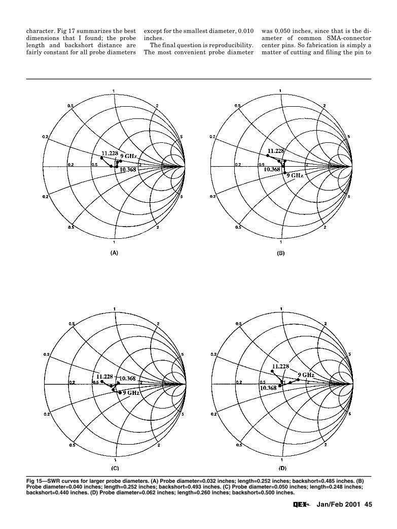
Fig 15—SWR curves for larger probe diameters. (A) Probe diameter=0.032 inches; length=0.252 inches; backshort=0.485 inches. (B)Probe diameter=0.040 inches; length=0.252 inches; backshort=0.493 inches. (C) Probe diameter=0.050 inches; length=0.248 inches;backshort=0.440 inches. (D) Probe diameter=0.062 inches; length=0.260 inches; backshort=0.500 inches.

character. Fig 17 summarizes the bestdimensions that I found; the probelength and backshort distance arefairly constant for all probe diameters

except for the smallest diameter, 0.010inches.

The final question is reproducibility.The most convenient probe diameter

was 0.050 inches, since that is the di-ameter of common SMA-connectorcenter pins. So fabrication is simply amatter of cutting and filing the pin to

46 Jan/Feb 2001

Fig 16—SWR curves for a very small probe diameter. Probe diameter=0.010 inches;length=0.265 inches; backshort=0.616 inches.

the desired length read from Fig 17. Icut up another hexagonal plumbing fit-ting to provide several flats for connec-tor mounting, then soldered one to theside of a piece of pipe as well as a smallbrass sheet for a backshort. I drilledand tapped holes in the flat for the con-nector and screwed it in place. The tran-sition worked well, providing an SWRof about 1.05 feeding a diagonal horn,so I assembled three more, using flatsfrom the hexagonal fitting. An alterna-tive construction technique is to use anSMA connector with a threaded body,which allows for some adjustment.Screwing the connector flange to a flatsurface is more robust and repeatable,however, and adjustment isn’t neces-sary if we have good dimensions.

I made the final measurements of thefour transitions from the coax inputusing an automatic network analyzer.Fig 19 shows the SWR of all four tran-sitions, each feeding a diagonal horn4

with SWR of about 1.06. The worst tran-sition has an SWR of about 1.11 at10.368 GHz, while the others are 1.05or lower. The SWR is under 1.5 from 9.8to 11+ GHz, a reasonable bandwidth. Tomeasure the loss, I connected two tran-sitions together with a simple plumb-ing joint slipped over them. The loss fora pair, shown in Fig 20, is 0.23 dB at10.368 GHz and under 0.3 dB from 9 to11 GHz. At 8.5 GHz, the cutoff fre-quency is obvious; waveguide makes anexcellent high-pass filter.

Scaling to Other FrequenciesI believe the transition should scale

well to other frequencies. The hardestpart is finding a pipe of suitable diam-eter, between 0.6 λ and 0.76 λ . Thenthe other dimensions can be scaled di-rectly to the ratio of pipe diameters,starting with a convenient probe di-ameter and taking the dimensionsfrom Fig 17. All dimensions must bescaled by the same ratio! If the probelength is made slightly long, it can betrimmed for best SWR.

Antenna ApplicationsThe real purpose of the circular

waveguide was to investigate antennaswith circular cross sections, particu-larly feed horns. I built several feedhorns for offset dishes, including theones shown in Fig 21: a conical horn,two large W2IMU dual-mode feed hornsand a rectangular horn feed for DSS off-set dishes. I also built a diagonal horn,5

a feed horn with a square cross sectionrotated so that the probe is parallelwith the diagonal. I made SWR andsun-noise measurements on these Fig 17—Circular waveguide-to-coax transition—best dimensions.

Jan/Feb 2001 47

Fig 18—A completed circular waveguide-to-coax transitions for 10 GHz.

Fig 19—Measured SWR for the completed 3/4-inch circular waveguide transitions with adiagonal-horn load.

Table 1—Dimensions two dual-mode feeds and the original W2IMU feed

Dimensions shown in wavelengths may be scaled to any frequency.f/D Flare B= C=

Aperture Diam. Output Length

0.55 30⋅ 1.31 λ 1.31 λ0.7 27.4⋅ 1.63 λ 2.8 λ0.8 24.9⋅ 1.79 λ 3.52 λ

Fig 20—Losses for a mated pair of 3/4-inch circular waveguide transitions.

horns as well as several surplus corru-gated horns with circular-waveguideinputs, which I machined to fit to 3/4-inch pipe. All the homemade horns hadSWRs better than 1.1. The diagonalhorn had particularly good SWR butdisappointing feed performance.

The two W2IMU dual-mode feedhorns are large versions, optimized foroffset dishes as described in theW1GHZ Microwave Antenna Book—Online.6 The original W2IMU feed7

provides best performance for an f/Daround 0.5. The two dual-mode hornsin Figure 21 are designed for largerf/D required for offset dishes: thelarger version in Figure 21 is dimen-sioned for f/D = 0.8 and the smallerfor f/D = 0.7. For a dual-mode horn toproperly illuminate a larger f/D, notonly must the aperture diameter in-crease, but also the length of the out-put section must increase and the flarehalf-angle must decrease. The dashedlines in Figure 22 illustrate thesechanges from the original version de-picted by the solid lines. The two largedual-mode feed horns provided thehighest efficiency I’ve measured todate, slightly higher than the rectan-gular feedhorn8 I designed for offsetdishes. One interesting result wasthat the efficiency was slightly higherwith circular polarization than withhorizontal polarization. The middlehorn in the table is currently workingwell feeding a one-meter offset dish aspart of my 10-GHz periscope9, 10 an-tenna system.

The dimensions for these two largerdual-mode feeds as well as the origi-nal W2IMU feed are shown in the fol-lowing Table 1. The dimensions areshown in wavelengths and may bescaled to any frequency. Dimension Ais not shown in the table; it is the di-ameter of the input circularwaveguide feeding the horn. The di-ameter of the input waveguide doesnot affect horn performance as long asonly the TE11 mode is propagated. Aswe saw previously, a range ofwaveguide diameters is usable.

48 Jan/Feb 2001

ConclusionsCircular waveguide for 10 GHz use

made from ordinary copper pipe is bothuseful and inexpensive. Using simpletest equipment and old-fashioned ex-perimental microwave engineering, Ihave found some good working dimen-sions for quality circular-waveguidecomponents. In the process, I learnedmore about circular waveguide. I hopethis demonstrates that fancy testequipment is not always necessary formicrowave work.

Notes1G. C. Southworth, Principles and Applica-

tions of Waveguide Transmission,(Princeton, NJ: Van Nostrand, 1950).

2D. M. Pozar, Microwave Engineering, sec-ond edition, (New York: Wiley, 1998) pp79-82.

3G. C. Southworth and A. P. King, “MetalHorns as Directive Receivers of Ultra-ShortWaves,” Proceedings of the IRE, February1939, pp 95-102. (reprinted in A. W. Love,Electromagnetic Horn Antennas, IEEE,1976, pp 19-26.)

4R. Chatterjee, Elements of Microwave Engi-neering, (Ellis Horwood Limited, 1986; NewYork: Halsted Press, 1986) pp 168-169.

5A. W. Love,“The Diagonal Horn Antenna,”Microwave Journal, March 1962, pp 117-122 (reprinted in A. W. Love, Electromag-netic Horn Antennas, IEEE, 1976, pp189-194.)

6You can view this at www.qsl.net/n1bwt/preface.htm; go to Chapter 6.5.

Fig 21—10-GHz feed horns for DSS offsetdishes.

Fig 22—The W2IMU dual-mode feed horn. See Table 1 for dimensions.

7R. H. Turrin, W21MU, “Dual Mode Small-Aperture Antennas,” IEEE Transactions onAntennas and Propagation, AP-15, March1967, pp 307-308. (reprinted in A. W. Love,Electromagnetic Horn Antennas, IEEE,1976, pp 214-215.)

8P. C. Wade, N1BWT, “More on ParabolicDish Antennas,” QEX, Dec 1995, pp 14-22.

9P. Wade, W1GHZ, “10 GHz without Feed-Line Loss,” Proceedings of the 24th East-ern VHF/UHF Conference, (Newington,Connecticut: ARRL, 1998), pp 227-237.

10P. Wade, W1GHZ, “Periscope AntennaSystems,” Proceedings of Microwave Up-date 2000, Trevose, Pennsylvania, 2000,pp 182-202.