Embed Size (px)
Citation preview
Understanding Housing Market Volatility
Joseph Fairchild∗ Jun Ma† Shu Wu‡
This version: April 2014
∗Bank of America, 100 North Tryon Street, Charlotte, NC 28202, phone: 949-422-0968,email: [email protected].
†Department of Economics, Finance and Legal Studies, Culverhouse College of Com-merce and Business Administration, University of Alabama, Auscalosa, AL 35487, phone:205-348-8985, email: [email protected].
‡Department of Economics, University of Kansas, Lawrence, KS 66045, phone: 785-864-2868, email: [email protected].
Abstract
The Campbell-Shiller present value formula implies a factor structure
for the price-rent ratio of the housing market. Using a dynamic factor
model, we decompose the price-rent ratios of 23 major housing markets
into a national factor and independent local factors, and we link these
factors to the economic fundamentals of the housing markets. We find
that a large fraction of housing market volatility is local and that the
national factor has become more important than local factors in driv-
ing housing market volatility since 1999, consistent with the findings
in Del Negro and Otrok (2007). The local volatilities mostly are due to
time-variations of idiosyncratic housing market risk premia, not local
growth. At the aggregate level, the growth and interest rate factors
jointly account for less than half of the total variation in the price-rent
ratio. The rest is due to the aggregate housing market risk premium
and a pricing error. We find evidence that the pricing error is related
to money illusion, especially at the onset of the recent housing market
bubble. The rapid rise in housing prices prior to the 2008 financial
crisis was accompanied by both a large increase in the pricing error
and a large decrease in the housing market risk premium.
Key words: dynamic factor model; housing market; price-rent ratio;
risk premium; money illusion
JEL Classifications: C32, G12, R31
1
1 Introduction
Housing markets are partially segmented. There does not exist a centralized
market for housing assets. Demographic changes, household preferences for
geographic locations and climate plus inelastic land supply can lead to het-
erogeneous regional price dynamics. Some existing studies, such as Gyourko,
Mayer and Sinai (2006) and Del Negro and Otrok (2007), have already ob-
served the price level and growth rate vary drastically across major U.S.
housing markets in the past few decades. As we can see in Table 1, for
example, the average annual nominal price change was 5.4% in New York
City but was only 2.7% in Kansas City during the period between 1979 to
2013. Moreover, the volatility of house prices also varies greatly across dif-
ferent cities. Table 1 shows the standard deviation of annual nominal price
changes for the same period. It was 8.1% in New York City but was 3.6% in
Kansas City. Table 2 reports similar statistics for the log price-rent ratios
of the same cities. For example, in New York City the log price-rent ratio
had an annual standard deviation of 24% while in Kansas City it was only
8.2% between 1979 to 2013.
On the other hand, all housing markets are obviously affected by a few
aggregate variables such as the monetary policy, mortgage market innova-
tions and national income. When the central bank lowers the key interest
rate, it could stimulate the demand for houses in all markets and have a
positive effect on housing prices. In fact Table 1 and Table 2 show that the
correlation among some housing markets can be very high (e.g. New York
City and Boston, Los Angles and Philadelphia).
In this study we use a dynamic factor model to decompose housing prices
into a common national factor and idiosyncratic local factors in order to
better understand the sources of housing market volatility. We treat a resi-
dential house as a dividend-paying asset and base our dynamic factor model
on the Campbell-Shiller log-linear approximate present value formula for
the price-dividend ratio (Campbell and Shiller, 1988). Such an approach
allows us to link the unobservable factors to the economic fundamentals of
2
the housing markets such as interest rates and expected rent growth.
Quantitatively distinguishing the national factor from local factors in the
housing markets is important. From the perspective of policy makers, for
instance, it is crucial to know if monetary policy was responsible for creating
a national housing market bubble by keeping the short-term interest rate
too low for too long, or if the increase in housing prices prior to the 2008
financial crisis instead reflected a collection of local bubbles. On the other
hand, identifying a market “bubble” is intrinsically difficult. An increase in
asset prices could be due to improved economic fundamentals as perceived by
investors or due to purely speculative activities. By linking the unobserved
price factors to economic fundamentals, our paper also seeks to distinguish
between the part of housing market volatility attributable to changes in
expected rent growth and the discount rate and the part that could be due
to speculation or pricing errors.
Given the importance of the housing sector in the aggregate economy,
there have been many studies on housing markets in recent years. For ex-
ample, Fratantoni and Schuh (2003) uses a heterogeneous-agent VAR to ex-
amine the effect of monetary policy on regional housing markets. Davis and
Heathcote (2005) points out that residential investment is more than twice
as volatile as business investment and leads the business cycle. Iacoviello
(2005) develops and estimates a monetary business cycle model with housing
sector. Brunnermeier and Julliard (2008) finds evidence that money illusion
can play an important role in fueling run-ups in housing prices. Stock and
Watson (2009) estimates a dynamic factor model with stochastic volatility
for building permits of the U.S. states from 1969-2007. Mian and Sufi (2009)
uses detailed zip-code level data to examine the role of subprime mortgage
credit expansion in fueling house price appreciation prior to the recent finan-
cial crisis. Kishor and Morley (2010) uses an unobserved component model
to estimate expectations of housing market fundamentals and investigate
the sources of aggregate housing market volatility. Ng and Moench (2011)
estimates a hierarchical factor model of the housing market and examines
the dynamic effects of housing market shocks on consumption. Favilukis
3
et al. (2011) argues that international capital flows played a small role in
driving the last house market bubble, and the key causal factor was instead
the cheap supply of credit due to financial market liberalization. Recently,
Sun and Tsang (2014) focus on the inference issues when studying sources to
the housing market volatility. Our paper contributes to this growing litera-
ture that seeks to understand the fundamental driving forces of the housing
market and its relationship to the aggregate economy.
Perhaps the closest studies to ours are Del Negro and Otrok (2007) and
Campbell et al. (2009). Del Negro and Otrok (2007) was among the first to
apply dynamic factor models to housing markets.1 In their study state-level
house price movements are decomposed into a common national component
and local shocks via Bayesian methods. They find that historically the lo-
cal factors have played a dominating role in driving the movement in house
prices in different states. But a substantial fraction of the recent increases in
house prices is due to the national factor. They further use a VAR to inves-
tigate the effect of monetary policy on housing markets. The key difference
between our study and Del Negro and Otrok (2007) is that we treat a house
as a dividend-paying asset and infer a factor structure for the price-rent
ratio based on the Campbell-Shiller log-linear present value formula. As a
result, we can explicitly link the unobserved factors to economic fundamen-
tals of the housing markets. The Campbell-Shiller formula has been widely
used to analyze the volatility of bond and equity markets. In an intriguing
study, Campbell et al. (2009) applied the same method to price-rent ratio
in housing markets.2 The ratio is split into the expected present values of
rent growth, the real interest rate and a housing risk premium. The study
found that the housing risk premium accounts for a significant fraction of
price-rent volatility. An important difference between our paper and Camp-
bell et al (2009) is that we are able to disentangle the relative importance
1Recent applications of dynamic factor models include Cicarelli and Mojon (2010) onglobal inflation, Ludvigson and Ng (2009) on bond risk premiums and Kose et al. (2003,2008) on global business cycles among many others. Forni et al. (2000) provides a thoroughanalysis of the identification and estimation of generalized dynamic factor models.
2Brunnermeier and Julliard (2008) also uses the same approach to isolate the pricingerror in the aggregate housing market due to money illusion.
4

of the common component in the price-rent ratios across individual markets
from idiosyncratic local factors using a dynamic factor model. We show
that this factor structure is an implication of the Campbell-Shiller present
value formula and both factors have similar representations. Moreover, we
show that a pricing error associated with money illusion is also important
in driving housing market dynamics.
To implement the Campbell-Shiller formula, we need to estimate ex-
pected future rent growth and the real interest rate. Another innovation of
our paper is that the forecasting vector auto-regression model (VAR) for fu-
ture rent growth and the real interest rate is embedded in a dynamic factor
model, and the two models are estimated jointly. The macro variables in the
VAR are correlated with the national factor of rent growth but are indepen-
dent of the local factors. Such a specification is important for appropriate
identification of the national and the local factors.
The rest of the paper is organized as follows. Section 2 describes our
model. Section 3 discusses the data and estimation strategy. Section 4
presents the main empirical results. Section 5 concludes.
2 Model
We treat a house as a dividend-paying asset and equate the house price
to the present value of the expected future rental income under rational
expectations.3 Following Campbell and Shiller (1988), we can write the
price-rent ratio as the sum of expected growth rate of rental income minus
the expected rate of return on the housing asset.
In particular, if Pi,t denotes the ex-dividend price of a housing asset in
market i at time t, Di,t+1 the rental income of the housing asset between t
3Using rent as an approximation of the dividend income of a housing asset, we implicitlyassume that individuals are indifferent between owning and renting. Glaeser and Gyourko(2007) points out that rental units in the housing markets tend to be very different fromowner-occupied units.
5
and t+1, let xi,t = log(
Pi,t
Di,t
), di,t = logDi,t and ri,t+1 = log
(Pi,t+1+Di,t+1
Pi,t
).
Under log-linear approximation, we have (ignoring constant terms):
xi,t = Et
∞∑τ=0
ρτ [∆di,t+1+τ − ri,t+1+τ ] (1)
where ρ = 1/(1+e−x), and x is the steady state price/rent ratio. The house
price today should equal the present value of expected future rent growth
minus the weighted average of expected future rates of return.
We assume in this study that the growth rate of rent in one market
consists of two components, a national factor that is common to all markets
and an independent local factor that is specific to market i. We can now
rewrite the standard Campbell-Shiller decomposition as
xi,t = Et
∞∑τ=0
ρτβd,i∆dt+1+τ+Et
∞∑τ=0
ρτ∆di,t+1+τ−Et
∞∑τ=0
ρτrf,t+1+τ−Et
∞∑τ=0
ρτeri,t+1+τ
(2)
where ∆dt is the national factor of rent growth rate and βd,i is the factor
loading for market i,4 ∆di,t is the idiosyncratic rent growth rate in market
i, rf,t is the real interest rate and eri,t is the excess rate of return in market
i, eri,t = ri,t − rf,t.
The last term in Equation (2) corresponds to the risk premium for in-
vesting in the housing market, which also can be written as the sum of two
components
Et
∞∑τ=0
ρτeri,t+1+τ = Et
∞∑τ=0
ρτβiert+1+τ + Et
∞∑τ=0
ρτ eri,t+1+τ (3)
The first part on the right side of the equation above can be thought of as the
national housing market risk premium and the second part an idiosyncratic
risk premium component that is specific to market i. This decomposition
can be justified as follows: if housing markets were fully integrated without
4For the purpose of identification we normalize the variance of the shock to the nationalfactor to unity. See more discussions below.
6
transaction cost and other frictions, it would then follow from the standard
asset pricing theory that Et(eri,t+1) = βiEt(ert+1), where ert+1 is the excess
return on a portfolio of housing assets that is perfectly negatively correlated
with the pricing kernel (or the stochastic discount factor).5 Of course much
evidence shows that housing markets are far from integrated and there are
many kinds of frictions in each market such as transaction costs, liquidity
constraints, etc. The second part on the right side of Equation (3) therefore
captures the expected excess rate return that is orthogonal to the aggregate
housing market risk premium. 6
In summary, the log-linear Campbell-Shiller present value formula im-
plies a factor structure for the price-rent ratios of the housing markets as
follows:
xi,t = xi,t + xi,t, i = 1, 2, ..., N (4)
where
xi,t = βd,iEt
∞∑τ=0
ρτ∆dt+1+τ − Et
∞∑τ=0
ρτrf,t+1+τ − βiEt
∞∑τ=0
ρτ ert+1+τ (5)
and
xi,t = Et
∞∑τ=0
ρτ∆di,t+1+τ − Et
∞∑τ=0
ρτ eri,t+1+τ (6)
As we will further show in Section 4.3, there could be an additional
pricing error term in Equation (5) if investors are not able to form rational
expectations of future real rent growth or the real interest rate. For example,
they may suffer from money illusion and mistakenly interpret a decline in
5Since we will estimate the risk premium as the residual term in the Campbell-Shilleridentity, we do not need to separately identify βi and Et(ert+1) but rather their product asa whole. Therefore as long as βi is constant or its time variations, if there are any, are notrelated with local state variables, our decomposition in (3) will remain valid. In Table 3 weemploy a quarterly data set for a small number of cities (due to limited data availabilityat the quarterly frequency) and report βi estimates over different sample periods. Theresults indicate that, although there are some time variations in βi for some cities, overallβi remains quite stable for most cities during our sample periods.
6One implicit assumption is that investors in different housing markets share the sameinformation set.
7
the nominal interest rate due to a change in inflation as a decrease in the
real interest rate (or equivalently they extrapolate the historical nominal
rent growth rate without taking into account changes in inflation). Under
money illusion, the price-rent ratio, xi,t, will include an extra term (a pricing
error) as follows,
xi,t =βd,iEt
∞∑τ=0
ρτ∆dt+1+τ − Et
∞∑τ=0
ρτrf,t+1+τ − βiEt
∞∑τ=0
ρτ ert+1+τ
+ (Et − Et)
∞∑τ=0
ρτrf,t+1+τ
(7)
where Et denotes people’s subjective expectation under money illusion, Et
denotes the rational expectation. Investors perceive the real interest rate to
be Et∑∞
τ=0 ρτrf,t+1+τ , while the actual real interest rate is Et
∑∞τ=0 ρ
τrf,t+1+τ .
The first part of Equation (7) corresponds to the “correct” or “true” house
value under rational expectations. If households underestimate the real in-
terest rate, for example, the observed house price xi,t will exceed its true
value by (Et − Et)∑∞
τ=0 ρτrf,t+1+τ . This pricing error will disappear if in-
vestors are able to correctly form rational expectations of future interest
rates (Et = Et). In our decomposition exercise, we will need to distinguish
empirically the pricing error from the risk premium term in the Campbell-
Shiller formula.7
3 Data and Estimation
In our model specification there are two types of unobserved factors: the
unobserved national and local factors for both rent growth and price-rent
ratio, and the unobserved agent’s expectations of future rent growth, future
7We focus on money illusion in the national factor here because there is no appealingreason to assume only households in one or some particular markets make this mistakewhile others do not. However, it is possible that money illusion effects may vary indifferent markets due to different inflation experience. In Section 4.4 we will also explorethe possibility of differential effects of the money illusion in different local markets.
8
interest rates and future excess returns or risk premiums. Typically the
unobserved national and local factors can be extracted from the observed
series by applying the type of Dynamic Factor Model (DFM) proposed in
Stock and Watson (1991), and the unobserved expected future variables can
be estimated by a VAR model that was first implemented in Campbell and
Shiller (1988) to study sources of price-dividend variation. We combine these
two lines of work and propose a novel VAR augmented DFM that allows us
to simultaneously decompose the observed series into the national and local
factors and obtain estimates of the expectations of future variables. Using
the estimated expectations along with the Campbell-Shiller present-value
accounting identity, we can further decompose the housing price variations
into movements in different economic fundamentals including time-varying
risk premiums.
Our data are semi-annual real rent growth and price-rent ratio of 23
metropolitan areas from 1979 to 2013. Real rent growth is obtained by de-
flating the nominal rent by the CPI. When applying the DFM to a real rent
growth we augment the DFM with a multivariate VAR that includes several
important macroeconomic variables (such as the interest rate) to allow for
potential interactions between the national factor of real rent growth and
observed macroeconomic variables. This is very important for several rea-
sons. First it ensures the appropriate identification of the local factor of
real rent growth in (6) which is supposed to be independent of the national
factor of rent growth and the real interest rate in (5). Second, as pointed
out by Engsted et al. (2012), a critical requirement for proper Campbell-
Shiller VAR decompositions is that the forecasting state variables should
include the current asset price. We address this issue by including the Case-
Shiller home price index as one of the macro variables in our model. Third,
the extra information contained in the macro variables can in principle im-
prove the forecasts of national real rent growth as well as the future interest
rate. More information on the data used in this paper can be found in the
appendix A.
Denote the real rent growth in the 23 metropolitan areas by ∆di,t. As-
9
sume a common national factor represented by ∆dt and the idiosyncratic
local factors denoted by ∆di,t. We use 2 lags for all dynamic factors since all
data are semi-annual and 2 lags appear sufficient to capture potential dy-
namics. Notice that all variables are demeaned before being used to estimate
the model. Specifically, the DFM part is set up as below:
∆di,t = βd,i∆dt +∆di,t, i = 1, 2, ..., 23 (8)
∆dt = ϕ1∆dt−1 + ϕ2∆dt−2 + ωt (9)
∆di,t = ψ1∆di,t−1 + ψ2∆di,t−2 + νi,t, i = 1, 2, ..., 23 (10)
where ωt and νi,t are independent Gaussian shocks.
We augment the above DFM with a VAR to allow the latent national
factor ∆dt to interact with four macroeconomic variables including the real
interest rate, rt, real GDP growth, gt, log changes in the Case-Shiller home
price index, st, and CPI inflation rate, πt:
Zt = Φ(L)Zt−1 + ξt (11)
where Zt = (∆dt, rt, gt, st, πt)′ and ξt = (ωt, εr,t, εg,t, εs,t, επ,t)
′. The variance
matrix of the innovations to the VAR is given by Σ. We also use 2 lags in
the VAR specification.
To estimate this VAR-DFM model we cast it in a state-space form. The
state-space representation of our model can be found in the appendix B. The
Kalman filter then is conveniently employed to obtain maximum likelihood
estimates of the hyper-parameters as in Kim and Nelson (1999). Once the
hyper-parameter estimates are found the flitering algorithm is invoked to
calculate the filtered estimates of the national and local factors: E[∆dt|It]and E[∆dt|It], i = 1, 2, . . . , 23. We rely on the filtered estimates in our
calculations of various pricing components since agents can only know the
information up to time t when pricing the housing assets. Iterating forward
the dynamics of the unobserved national factor and observed macroeconomic
variables, we can derive the growth component and interest rate component
10
in the Campbell-Shiller decomposition (5) as follows:
Et
∞∑τ=0
ρτ∆dt+1+τ = e′1 · F · (I − ρF )−1 ·Wt (12)
Et
∞∑τ=0
ρτrt+1+τ = e′3 · F · (I − ρF )−1 ·Wt (13)
where Wt = (∆dt,∆dt−1, rt, rt−1, gt, gt−1, st, st−1, πt, πt−1)′, i.e., the second
half of the state variables in the transition equation (22) in Appendix B; F
is the corresponding companion matrix in the VAR model. ej is a selection
column vector which has 1 as the j-th element and zero elsewhere. In the
same way, the idiosyncratic local growth component Et∑∞
τ=0 ρτ∆di,t+1+τ
can be computed relatively easily since it is by construction independent of
the macroeconomic variables.
The aggregate and local risk premium components are obtained as the
residual terms in the Campbell-Shiller accounting identity (5) and (6), re-
spectively. We first apply the DFM to the log price-rent ratio and extract
the national and local factors from this series.8 Assume each price-rent ratio
is the sum of the unobserved national factor and local factor:
xi,t = βx,ixt + xi,t, i = 1, 2, . . . , 23 (14)
and the national and local price-rent ratios both follow the stationary AR(2)
processes:
xt = α1xt−1 + α2xt−2 + et, et ∼ i.i.d. N(0, σ2e) (15)
xi,t = γi,1xi,t−1 + γi,2xi,t−2 + ςi,t, ςi,t ∼ i.i.d. N(0, σ2ς,i) (16)
Again, the national and local factors are orthogonal to each other for
identification purposes following Stock and Watson (1991). This model
8Before applying the DFM to the log price-rent ratio data, we ran a panel unit roottest and rejected the unit root hypothesis. This is consistent with the finding in Ambroset al (2011) that house price and rent are cointegrated.
11
again can be put into its state-space form and the estimation is done by
following Kim and Nelson (1999). The risk premium term is then obtained
by subtracting the rent growth and interest rate components from the price-
rent ratio.
Also notice that in the dynamic factor models, the scale of the common
factor and the factor loading are not identified independently. We normalize
the standard deviation of the shocks to the common factor to be 1 to achieve
identification.
4 Results
4.1 Factor Decomposition
We first estimate a dynamic factor model of the semi-annual log price-rent
ratios of the 23 cities in our sample. The model decomposes each price-
rent ratio into a common national factor and a local factor. The model is
estimated for three sample periods, 1979 - 2013, 1979 - 1999S1 and 1999S2 -
2013. Table 4 summarizes the fractions of housing market volatility due to
local factors. We measure the volatility of a housing market by the standard
deviation of the semi-annual log price-rent ratio. We find that across the
23 cities local factors drive a significant portion of the total volatility in the
housing markets. As Table 4 shows, for the whole sample period of 1979
- 2013, an average of 37% of the total volatility of the housing markets is
attributable to local factors. In some cities, the local factor shares are more
than 60%. Across the two sub-sample periods, while local factors account
for more than half of housing market volatility during 1979 - 1999S1, local
factor’s impact has become much smaller since 1999. Almost 65% of the
volatility of the housing markets can be attributable to a common national
factor during 1999S2 - 2013. These results are consistent with those of Del
Negro and Otrok (2007), which finds that historically movements in house
prices were mainly driven by local components and that national factor has
played a bigger role in recent years. Figure 1 plots the estimated national
12
factor of the price-rent ratio together with the Case-Shiller house price index
(normalized by the CPI index).9 We can see that these two series track
each other closely with a correlation coefficient of over 80%. Our series of
the national factor of the price-rent ratio is also very similar to the one
estimated by Davis et al. (2008). This confirms that the dynamic factor
model provides a good summary of housing market movements.
4.2 Local Factor Shares
Table 4 also shows that the local factor shares vary greatly from city to
city. For example, while local factor contributes more than 60% of the
total volatility of the price-rent ratio in Houston, the local factor share is
only around 15% in St Louis. The log-linearized Campbell-Shiller present
value formula provides insights about what drives these local volatilities.
The Campbell-Shiller formula is an accounting identity that expresses log
price-rent ratio as a sum of two components: the present value of expected
future rent growth rates and the present value of expected future discount
rates. House prices increase today either because people expect higher future
rent growth or a lower discount rate or both. As we have demonstrated in
Section 2, the growth component can be further decomposed into a common
national growth factor and an independent local growth factor. The discount
rate component can be thought of as consisting of three factors, a risk-free
interest rate, an aggregate or national risk premium which is common to
all cities, and an idiosyncratic local risk premium. Therefore, in cites where
local factors contribute a large share to housing market volatility there must
be either volatile local growth or volatile local risk premiums or both. In
Table 5 we report the standard deviations of local rent growth and local risk
premiums (see below for more on the estimation of different components
in the Campbell-Shiller accounting identity). We can see that on average
local risk premiums are about 2 times more volatile than local rent growth
between 1979 and 2013. We have very similar results for the two sub-sample
9The semi-annual data of Case-Shiller index started from 1987.
13
periods (1979-1999S1 and 1999S2-2013). Notice that the lower volatilities
of local growth and local risk premium in the second half of the sample
(1999S2-2013) are consistent with declining local factor shares of price/rent
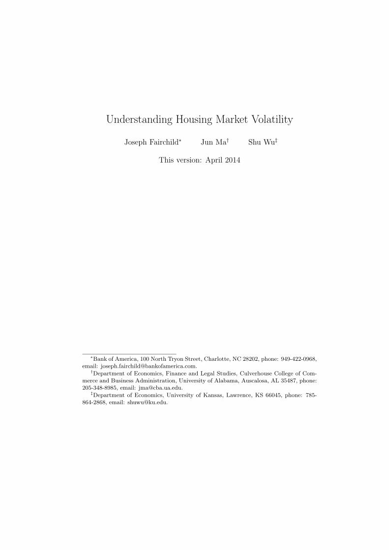
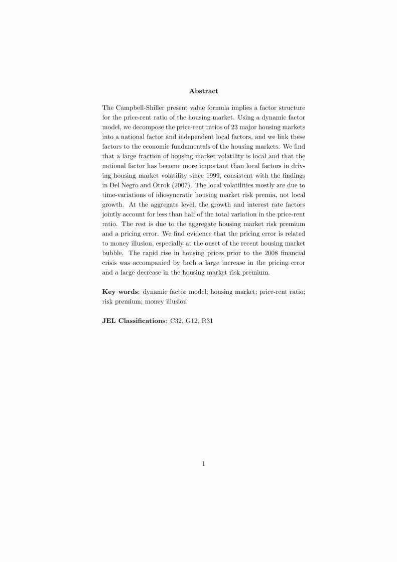
volatility documented in Table 4. In Figure 2 we plot the scatter graph of
local factor shares of the volatility of price-rent ratio against the standard
deviations of local risk premiums. In Figure 3 we plot a similar graph with
the standard deviations of local rent growth instead. We can clearly see from
these two figures that the local factor shares are closely associated with the
volatility of local risk premiums. Variation in the local growth volatility has
some, but very limited, explanatory power for the local factor shares. Simple
regressions of local factor shares on the volatility of local growth and the
volatility of local risk premium (Table 6) confirm these results. During the
whole sample period as well as the two sub-sample periods, the regression
coefficient on the volatility of local risk premium is highly significant and
R2 is high. The coefficient on local growth is not significant (except in the
first sample period) with low R2. Cities with high local factor shares are
those with large time variations in local risk premiums.
To study potential sources of local factor share variations across cities, in
Table 7 we report the results of regressing the volatility of local risk premium
on an index of local regulations. We use two indexes for local regulation.
One is the Wharton Residential Land Use Regulation Index (WRLURI)
and other is the index of housing supply regulation created by Sakes (2008).
Both index are standardized to have a mean of zero and a standard deviation
of one and are increasing in the degree of regulation. The two indexes have
a positive correlation of 0.60 (see more in the Data appendix). Table 7
shows that variations in local risk premiums are negatively correlated with
the degree of local regulations. Cities have higher level of regulation tend to
have less volatile housing market risk premiums. And this negative relation
is especially strong in the second half of the sample period (1999-2013).
Since time variations in risk premium must be due to either time-varying
risk of housing markets or time-varying risk aversion of investors, the results
in Table 7 suggest that more stingent local regulations may have helped
14
mitigate speculative activities in some housing markets during the 1999-
2013 sample period.
4.3 Economic Fundamentals of Housing Markets
We next examine the economic fundamentals that underlie the national and
local factors of house price-rent ratios. Using the Campbell-Shiller log-linear
present-value formula, we are able to equate the national factor of the log
price-rent ratio to the sum of the present value of the expected national
growth rate in rent, the present value of the expected real interest rate and
an aggregate risk-premium term. Similarly, the local factor of a price-rent
ratio can be written as the sum of the present value of the expected local
growth rate in rent and a local risk premium term. We embed a vector
regression model into a dynamic factor model of rent growth rates. This
allows us to obtain joint estimates of the national and local factors of rent
growth as well as expected future interest rates. The national and local
risk premium terms are then obtained as residuals in the Campbell-Shiller
accounting identity using our previous estimates of the national and local
factors of the log price-rent ratios.
Table 8 shows the volatilities of different components of the national
housing market.10 For the whole sample period of 1979 - 2013, the inter-
est rate term has the largest standard deviation of 22.49% among the three
economic variables underlying the national housing market. The risk pre-
mium term has a standard deviation of 15.66%, indicating strong evidence
of time-varying risk premiums in the aggregate housing market. The growth
term is the least volatile variable with a standard deviation of 7.87%. These
three variables are laso highly correlated. The growth term and real interest
rate are positively correlated. The risk premium is negatively correlated
10Since dynamic factor models can’t independently identify the variance of a com-mon factor and the factor loadings, we report in Table 8 the cross-section average of
the national factors of rent growth and risk premium,(∑
i βd,i
N
)Et
∑∞τ=0 ρ
τ∆dt+1+τ and(∑i βi
N
)Et
∑∞τ=0 ρ
τ∆ert+1+τ
15
with both the growth term and real interest rate.11 Across the two sub-
sample periods (1979 - 1999S1 and 1999S2 - 2103), however, there are some
major differences. In particular, risk premium becomes the most volatile
component of the aggregate housing market relative to the interest rate and
the growth components during 1999-2013 and is (weakly) positively corre-
lated with the growth component. The interest rate term became much less
volatile during 1999-2013 probably due to long period of zero interest rate
policy since the financial crisis of 2008.
To assess the impact of the economic fundamentals on housing markets,
we report in Table 9 the results from simple regressions of log price-rent
ratios on the growth and interest rate variables during 1979-2013. Notice
that our estimates of the national growth factor and the real interest rate
term are obtained from a separate dynamic factor model than the one for
price-rent ratio, and the risk premium is obtained as the residual term in the
Campbell-Shiller accounting identity. Therefore a meaningful regression is
one that only includes the growth and interest rate variables. Table 9 shows
that the growth component has little explanatory power for the variations
of the aggregate housing market. The interest rate alone accounts for about
42% of the variation in the aggregate log price-rent ratios, and the growth
and interest rate variables jointly explain up to 44% of the total variation
in the aggregate log price-rent ratios. Moreover, consistent with standard
economic theory, a higher expected real interest has a significantly negative
effect on house prices. In contrast, the regression coefficient on the growth
component is not significant and has the “wrong” sign. The regression
result indicates that a large portion (more than 50%) of the variation in
the national house market is due to changes in the aggregate risk premium
term.
Table 9 also reports the results from regressing local price-rent ratios
on local growth variables. In contrast to the aggregate housing market,
11The negative correlation between the housing market risk premium and growth isconsistent with the counter-cyclical risk premiums in the stock market documented inmany studies such as Campbell and Cochrane (1999).
16
local growth does have some explanatory power for local price/rent ratios
in a few cities such as New York City and Houston. The R2 of these local
regressions, however, are on average very small. This suggests that the
idiosyncratic volatilities in local housing markets are mostly due to time-
variation in local risk premiums, consistent with the result on the local factor
shares in the previous section. Combining the results from local and national
regressions, it seems safe to conclude that variation in risk premiums is the
most important factor that drives housing market volatility. Changes in the
interest rate have the expected, but limited, direct effect on housing market
volatility. Regressions based sub-sample data yield a similar conclusion.12
4.4 Housing Market Risk Premiums and the Pricing Error
The residual term from the Campbell-Shiller present value formula (5) is the
expected excess return or risk premium in the aggregate housing market,
Et∑∞
τ=0 ρτ ert+1+τ . This is a valid decomposition if investors have rational
expectations and the transversality condition holds, i.e., limT→∞ ρTEtxt+T =
0, where xt is the national factor of log price-rent ratio. In general, however,
the residual term from the Campbell-Shiller formula may include a pricing
error. This pricing error can arise because either investors hold irrational
expectations or there is a speculative bubble that violates the transversality
condition. We now rewrite the Campbell-Shiller present value formula as
xi,t = βd,iEt
∞∑τ=0
ρτ∆dt+1+τ−Et
∞∑τ=0
ρτrf,t+1+τ−βiEt
∞∑τ=0
ρτ ert+1+τ+ limT→∞
ρTEtxi,t+T
(17)
or
xi,t = βd,iyt − lt − βiηt + νi,t (18)
where yt, lt and ηt are, respectively, the expected rent growth, the real
interest rate and the risk premium, and νi,t denotes a possible pricing error
12Kishor and Morley (2010) reports a similar finding that variation in risk premiums ex-plains a large fraction of housing market volatility. Cochrane (2011) argues that most assetmarket puzzles and anomalies are related to large discount-rate/risk premium variation.
17

in the housing market. Our dynamic factor models produce estimates of
xi,t, βd,iyt and lt, and the residual term from the account identity (18) now
contains two components, the risk premium and the pricing error, βiηt and
νi,t.
It is well documented that the excess return in the equity market can be
predicted by some state variables such as yield spread and dividend yield.
To distinguish between the risk premium and the pricing error in the ag-
gregate housing market, we project via OLS regression the residual term
from the Campbell-Shiller formula (18) onto the same state variables that
are known to predict stock market returns as well as the national house
price/rent ratio. We interpret the fitted value as the national housing mar-
ket risk premium and the OLS residual as the aggregate pricing error. No-
tice that in dynamic factor models we can not separately identify the factor
loadings and the standard deviation of a national factor. We again use the
cross-section average of the Campbell-Shiller residuals from the 23 cities in
the OLS regression. The results are reported in upper panel of Table 10.
We can see that both the yield spread (the difference between the yield on
Treasury bonds and that on Treasury bills), S&P 500 price/dividend (or
price/earning) ratio and housing market price/rent ratio are significant pre-
dictors of the housing market returns. The R2 from the OLS regression is
high, indicating a large part of the Campbell-Shiller residual is the housing
market risk premium that varies over time. Nonetheless the pricing error
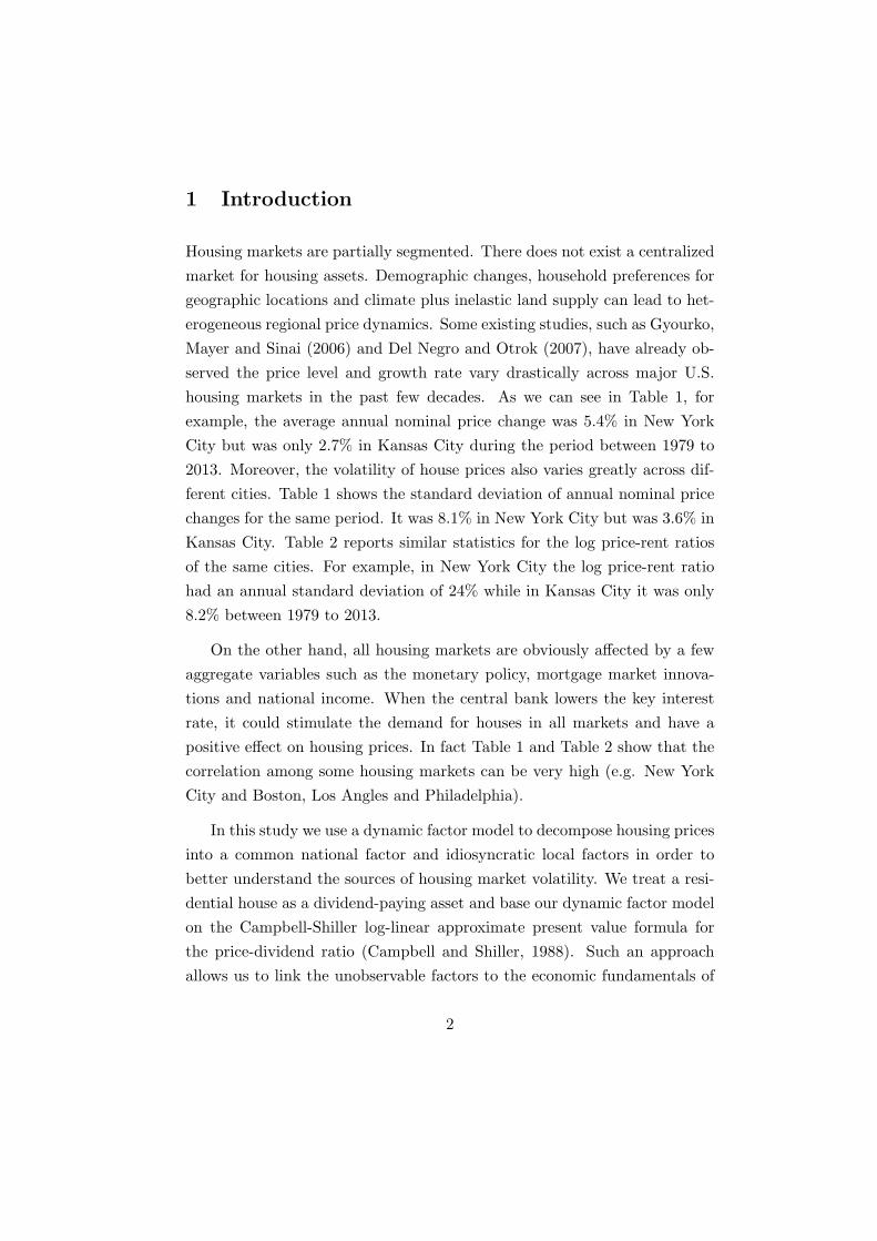
is also significant. The estimated housing market risk premium and pricing
error are plotted in Figure 4. We can clearly see that during the housing
market frenzy between 2000 and 2007, there was a large increase in the
pricing error, νt, and an even larger decrease in the risk premium, ηt, both
contributing to the sharp increase housing market prices before the 2008
financial crisis. In contrast, during the early sample period (1979 to 1985),
the risk premium was increasing while the pricing error remains roughly the
same. As a result, housing prices declined during that period (Figure 1).
It is interesting to notice that in the risk premium regression (the upper
panel of Table 10), the coefficients on the yield spread and S&P 500 log
18
price/dividend ratio both are positive while the coefficient on log house
price/rent ratio is negative. The negative coefficient on house price/rent
ratio implies that a higher house price must signal lower excess returns on
housing asset. A large positive yield spread indicates that interest rates are
likely to rise in the future, and rising interest rates decrease values of long-
term assets such as houses. Therefore a large yield spread increases the risk
to participate in the housing market, resulting in a higher risk premiums.
On the other hand, it is well known that the dividend yield has strong
forecasting power for future stock returns. For example Cochrane (2011)
shows that a one percentage point increase in the dividend yield forecasts
a nearly four percentage point higher excess return in the stock market.
In states where the dividend yield is high (hence log price/dividend ratio
is low), investors perceive a larger risk in the stock market and demand
a higher expected return. As a result they are more willing to accept a
lower expected return in the housing market. A higher dividend yield (or
a lower price/dividend ratio) in the stock market predicts lower returns in
the housing market. Housing assets seem to provide a hedge against stock
market risk. Of course, such interpretations are subject to the caveat that
part of the estimated risk premium may actually be the projection of the
pricing error on the state variables or that the three state variables fail to
capture all the variation of the housing market risk premium.
The orthogonal residual term from the above OLS regression can be
interpreted as an estimate of the aggregate housing market pricing error.
One possible source of the pricing error is money illusion. For example,
Modigliani and Cohn (1979) argues that investors may fail to distinguish
between the real interest rate and nominal interest rate. They may interpret
a decline in the nominal interest rate due to changes in inflation as a decline
in the real interest rate, and therefore bid up the real housing price. As
pointed out by Brunnermeier and Julliard (2008), in the simplest case with
constant real rents and real interest rates, the price-rent ratio will be simply
determined as:P
D=
∞∑τ=1
1
(1 + r)τ=
1
r(19)
19
where r is the real interest rate. Under money illusion, however, investors
would value the housing asset as
P
D=
∞∑τ=1
1
(1 + i)τ=
1
i(20)
where i is the nominal interest rate. And if i declines due to a reduction
in inflation, the price-rent ratio will increase even if the real interest rate
remains constant.
To see if the estimated pricing error is indeed related to money illusion,
we run an OLS regression of the pricing error on the inverse of the nominal
interest rate. The results are reported in the second panel of Table 10.
We can see that the estimated pricing error is indeed positively related to
the inverse of the nominal interest rate. The regression coefficient is highly
significant and R2 is above 20%. We also control for inflation or change in
inflation in the regression and we obtain the same result. Notice that the R2
of the regressions are not very high, suggesting that money illusion may not
be the only source of the pricing error. This is in contrast to the result in
Brunnermeier and Julliard (2008) where the pricing error is almost entirely
explained by money illusion.
The results of our dynamic factor model suggest a potential change of
the factor share structure around 1999 (see Table 4) and this may affect the
results about risk premium and pricing error above. To address this issue,
we estimate the dynamic factor model using data from 1999 to 2013 only and
repeat the same risk premium/pricing error regressions as above. We report
the results in Table 11. We can see that all the coefficients from the risk
premium and the pricing error regressions remain similar as before. Both
stock market price dividend ratio and housing market price rent ratio have
significant forecasting power for future excess returns in housing market.
Pricing error is still positively correlated with the inverse of nominal interest
rate, suggesting a money illusion effect. If we plot the fitted housing market
risk premium we see a similar decrease prior to the financial crisis. The
20
R2 from the risk premium regression, however, become much bigger than
before. This implies that the pricing error may be smaller than what the
whole-sample-estimation indicates. Another reason for the high R2 is that
the regression is run over a shorter sample period.
In local markets, local risk premiums are identified by the residuals of a
similar local Campbell-Shiller identity (6), where local log price/rent ratio,
xi,t, and expected local real rent growth, Et∑∞
τ=0 ρτ∆di,t+1+τ , can be es-
timated based on our dynamic factor model and the forecasting VAR. It is
possible that the residual term also includes a pricing error if the expecta-
tion of local real rent growth is distorted by local inflation. Separating local
pricing errors from local risk premiums is more difficult because it is not
obvious what local state variables are appropriate for identifying local risk
premium. We conjecture that investors in cities that experience higher local
inflation are more likely to have distorted expectation of real rent growth
and the presence of such pricing errors will increase the volatility of the local
Campbell-Shiller residual term (or the estimated local risk premiums). In
Table 12 we report the results from regressing the cross-section of volatili-
ties of the estimated local risk premiums on the levels of local CPI inflation
(excluding shelter) for three periods respectively, 1979 - 2013, 1979-1999
and 1999-2013. In all three periods, the volatility of the estimated local
risk premium is indeed positively correlated with the level of local inflation,
although the regression coefficient is not significant for the whole or the sec-
ond half of the sample period. During 1979-1999 where the average inflation
is much higher than the latter period, however, the regression coefficient is
significant and the R2 is more than 13%. These results indicate that pricing
errors from money illusion may be present at local level as well and investors’
past experience may play an important role in shaping their expectations of
future growth or discount rate.
21
5 Conclusions
This paper is an empirical analysis of housing market dynamics. The hous-
ing asset is probably the single most important component of an average
household’s financial portfolio. Housing market movements also have great
impacts on macroeconomic fluctuations. Compared to equity and bond
markets, however, there have been relatively fewer studies on the nature
and sources of housing market volatility. We contribute to a growing lit-
erature on housing markets by estimating a dynamic factor model of the
price-rent ratios of 23 major metropolitan areas of the U.S. The model al-
lows us to disentangle the common and idiosyncratic local components of
housing market volatility. We find that a large fraction of housing market
volatility is local, although the impact of local factors has become smaller
after 1999. Our dynamic factor model is based on a present-value represen-
tation of the price-rent ratio of the housing asset and is jointly estimated
with a forecasting VAR that includes important macroeconomic variables.
This approach enables us to relate otherwise unobservable latent factors to
economic fundamentals of the housing markets. Our results indicate that at
both the local and the aggregate levels time-variation in risk premiums is
the most important source of housing market volatility. Interest rates play a
smaller role in driving the movements of the housing markets. Nonetheless,
changes in the interest rate can have a direct and indirect impact on the
housing market. A decrease in the interest rate directly lowers the discount
rate, and therefore pushes up home prices. Moreover, a sharp decline in
the interest rate can also fuel housing market speculation through a money
illusion effect. We find evidence that the housing market bubble leading to
the 2008 financial crisis was indeed accompanied by both a large decrease in
the housing market risk premium and a large increase in the pricing error
associated with money illusion.
22
References
[1] Ambrose, B.W., P. Eichholtz and T. Linderthal, 2011, “House Prices
and Fundamentals: 355 Years of Evidence”, working paper, Pennsylva-
nia State University.
[2] Brunnermeier, M. K. and C. Julliard, 2008, “Money Illusion and Hous-
ing Frenzies”, The Review of Financial Studies, 21, 135-180.
[3] Campbell, J. and R. Shiller, 1988, “The Dividend-Price Ratio and Ex-
pectations of Future Dividends and Discount Factors”, Review of Fi-
nancial Studies, 1, 195-228.
[4] Campbell, J. and J. Cochrane, 1999, “By force of habit: A
consumption-based explanation of aggregate stock market behavior”,
Journal of Political Economy 107, 205-251.
[5] Campbell, S. D., M. A. Davis, J. Gallin, and R. F. Martin, 2009, “What
Moves Housing Markets: A Variance Decomposition of the Rent-Price
Ratio”, Journal of Urban Economics, 66, 90-102.
[6] Ciccarelli, M. and B. Mojon, 2010, “Global Inflation”, Review of Eco-
nomics and Statistics, 92, 524-535.
[7] Cochrane, J.H., 2011, “Discount Rates”, The Journal of Finance, 66,
1047-1108.
[8] Davis, M.A. and J. Heathcote, 2005, “Housing and the Business Cycle”,
International Economic Review, 46, 751-784.
[9] Davis, M.A., A. Lehnert and R.F. Martin, 2008, “The Rent-Price Ra-
tio for the Aggregate Stock of Owner-Occupied Housing”, Review of
Income and Wealth, 54, 279-284.
[10] Del Negro, M. D. and C. Otrok, 2007, “99 Luftballons: Monetary Policy
and the House Price Boom Across U.S. States”, Journal of Monetary
Economics, 54, 1962-1985.
23
[11] Engsted, T., P.Q. Thomas and C. Tanggaard, 2012, “Pitfalls in VAR
based Return Decompositions: A Clarification”, Journal of Banking
and Finance, 36, 1255-1265.
[12] Favilukis, J., D. Kohn, S.C. Ludvigson and S. van Nieuwerburgh, 2011,
“International Capital Flows and House Prices: Theory and Evidence”,
working paper, New York Univesity.
[13] Forni, M., M. Hallin, M. Lippi and L. Reichlin, 2000, “The General-
ized Dynamic Factor Model: Identification and Estimation”, Review of
Economics and Statistics, 82, 540-554.
[14] Fratantoni, M. and S. Schuh, 2003, “Monetary Policy, Housing, and
Heterogeneous Regional Markets”, Journal of Money, Credit and Bank-
ing, 35, 557-589.
[15] Glaeser, E.L and J. Gyourko 2007, “Arbitrage in Housing Markets”,
NBER Working Paper 13704.
[16] Gyourko, J., C. Mayer, and T. Sinai, 2006,“Superstar Cities”, NBER
Working Paper 12355.
[17] Iacoviello, M., 2005, “House Prices, Borrowing Constraints, and Mon-
etary Policy in the Business Cycle”, American Economic Review, 95,
739-764.
[18] Kim, C.J. and C. R. Nelson, 1999, State-Space Models with Regime
Switching: Classical and Gibbs-Sampling Approaches with Applications,
The MIT Press.
[19] Kishor, N.K. and J. Morley, 2010, “What Moves the Price-Rent Ratio:
A Latent Variable Approach”, working paper, University of Wisconsin-
Milwaukee.
[20] Kose, A., C. Otrok and C. Whiteman, 2003, “International Business
Cycles: World, Region and Country Specific Factors”, The American
Economic Review, 93, 1216-1239.
24
[21] Kose, A., C. Otrok and C. Whiteman, 2008, “Understanding the Evolu-
ation of World Business Cycles”, Journal of International Economics,
75, 110-130.
[22] Ludvigson, S.C. and S. Ng, 2009, “Macro Factors in Bond Risk Premia”,
Review of Financial Studies, 22, 5027-5067.
[23] Mian, A. and A. Sufi, 2009, “The Consequences of Mortgage Credit
Expansion: Evidence from the U.S. Mortgage Default Crisis”, Quarterly
Journal of Economics 124, 1449-1196.
[24] Modigliani, F. and R. Cohn, 1979, “Inflation, Rational Valuation and
the Market”, Financial Analysts Journal, 37, 24-44.
[25] Ng, S. and E. Moench, 2011, “A hierarchical factor analysis of U.S.
housing market dynamics,” Econometrics Journal, 14, 1-24.
[26] Saks, R.E., 2008, “Job Creation and Housing Construction: Constraints
on Metropolitan Area Employment Growth”, Journal of Urban Eco-
nomics 64, 178-195.
[27] Sun, X. and K.P. Tsang, 2014, ”Do More Regulated Housing Markets
Behave Differently?” working paper, Virginia Tech.
[28] Stock, J. H. and M. W. Watson, 1991, “A Probability Model of the Co-
incident Economic Indicators”, in Leading Economic Indicators: New
Approaches and Forecasting Records, ed. K. Lahiri and G. H. Moore.
Cambridge University Press, 63-89.
[29] Stock, J. H. and M. W. Watson, 2009, “The Evolution of National and
Regional Factors in U.S. Housing Construction”, in Volatility and Time
Series Econometrics: Essays in Honour of Robert F. Engle, T. Boller-
slev, J. Russell and M. Watson (eds), 2009, Oxford: Oxford University
Press.
[30] Shiller, R., 2005, Irrational Exuberance, second ed. Princeton University
Press, Princeton, NJ.
25
A Data
Rent growth. Nominal rent indexes are the rent of primary residence for
major U.S. metropolitan areas from the Bureau of Labor Statistics (BLS).13
The beginning periods and the reporting frequencies of these indexes vary
substantially for different cities and also over time for the same city. To
include as much data as possible in the time dimension and to include as
many cities as possible to span wide geographic regions, we follow Camp-
bell et al. (2009) and focus on the semi-annual frequency. For many cities
included in our study due to the inconsistency of reporting frequency of
the rent data over time and across cities we take averages of monthly ob-
servations when necessary to convert to the semi-annual observations. Our
sample period starts from 1979S1 and ends in 2013S1. This leaves us with a
set of 23 cities: New York City, Philadelphia, Boston, Pittsburgh, Chicago,
Cincinnati, Cleveland, Detroit, Kansas City, Milwaukee, Minnesota, At-
lanta, Houston, Los Angeles, Portland, San Francisco, Seattle, St.Louis,
Dallas, Miami, Denver, Honolulu, and San Diego. Evidently the data covers
most major cities ranging from the east coast to the midwest and west coast.
The nominal rent then is deflated by the consumer price index (CPI). Real
rent growth is the difference of the logarithms of real rent index.
Log price-rent. Nominal housing price indexes are the repeat-transaction
house price indexes from the Federal Housing Finance Agency (FHFA). We
take averages of monthly observations to convert to semi-annual ones. We
then divide the nominal housing price by the nominal rent and take the
logarithm to get the log price-rent ratio. Notice that since both price and
rent are indexes, the log price-ratio deviates from its true value by a constant.
This caveat, however, won’t affect our analysis of housing market volatility.
Other macroeconomic variables. Real GDP growth rate and the con-
sumer price index are from the FRED website. The Case-Shiller home price
13These indexes are the Consumer Price Index (CPI) rent components whose construc-tion has been criticized by a number of studies such as the Boskin Commission Report.While we are aware of this problem, these indexes are the only rent series available andare often used in studies such as Campbell et al. (2009).
26
index is taken from Robert Shiller’s book Irrational Exuberance, available on
Shiller’s website. The real interest rate used in our estimation is the short
rate minus the CPI inflation rate. The short rate is the one-year Treasury
bill rate and the long rate is the ten-year Treasury bond rate, and both
are from the FRED website. For all series, we convert either quarterly or
monthly observations of the macroeconomic variables to semi-annual ones
by taking the average.
Indexes of local regulation used in our study are Wharton Residential
Land Use Regulation Index (WRLURI) based on a 2005 survey and the index
of housing supply regulation created by Sakes (2008) for the late 1970s and
1980s. Both indexes have a mean zero and a standard deviation of one. A
larger index value indicates a higher degree of regulation. A market with
an index value of positive one is one standard deviation above the national
mean.
B The State Space Representation
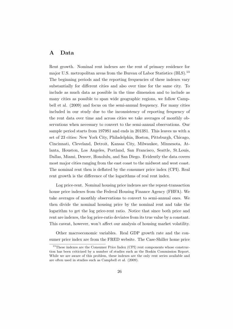
In this appendix, we describe the state-space representation of our model for
rent growth. We cast the model as specified by Equations (8), (9), (10), and
(11) in a state-space representation with the measurement and transition
equations as follows.
Measurement equation:
Ut = MYt (21)
27
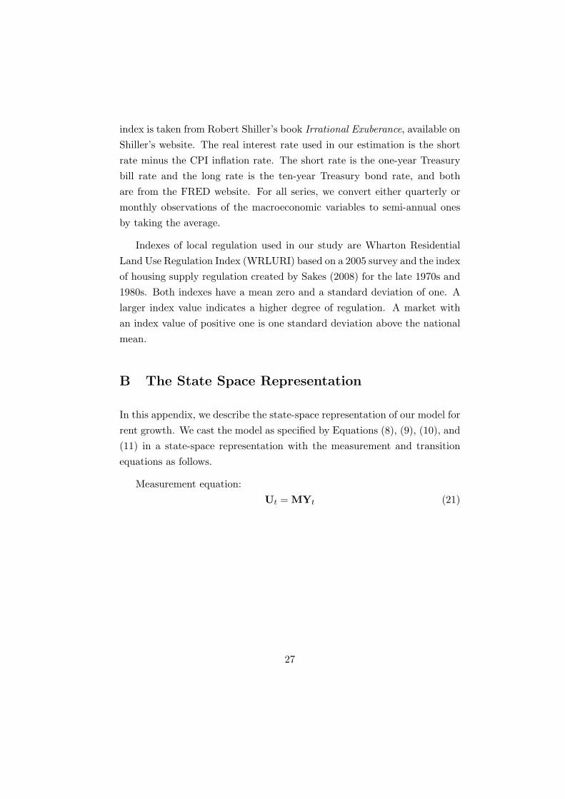
where
Ut =
∆d1,t...
∆d23,t
rt
gt
st
πt
, M =
1 0 · · · 0 0 βd,1 0 0 0 0 0 0 0 0 0...
......
...
0 0 · · · 1 0 βd,23 0 0 0 0 0 0 0 0 0
0 0 0 0 0 0 0 1 0 0 0 0 0 0 0
0 0 · · · 0 0 0 0 0 0 1 0 0 0 0 0
0 0 · · · 0 0 0 0 0 0 0 0 1 0 0 0
0 0 · · · 0 0 0 0 0 0 0 0 0 0 1 0
Transition equation:
Yt = ΛYt−1 +Θt (22)
where
Yt =
∆d1,t
∆d1,t−1
...
∆d23,t
∆d23,t−1
∆dt
∆dt−1
rt
rt−1
gt
gt−1
st
st−1
πt
πt−1
, Θt =
ν1,t
0...
ν23,t
0
ωt
0
εr,t
0
εg,t
0
εs,t
0
επ,t
0
28
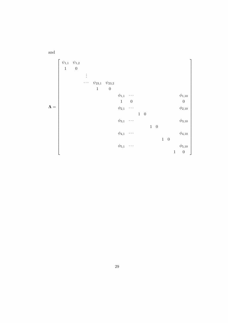
and
Λ =
ψ1,1 ψ1,2
1 0...
· · · ψ23,1 ψ23,2
1 0
ϕ1,1 · · · ϕ1,10
1 0 0
ϕ2,1 · · · ϕ2,10
1 0
ϕ3,1 · · · ϕ3,10
1 0
ϕ4,1 · · · ϕ4,10
1 0
ϕ5,1 · · · ϕ5,10
1 0
29
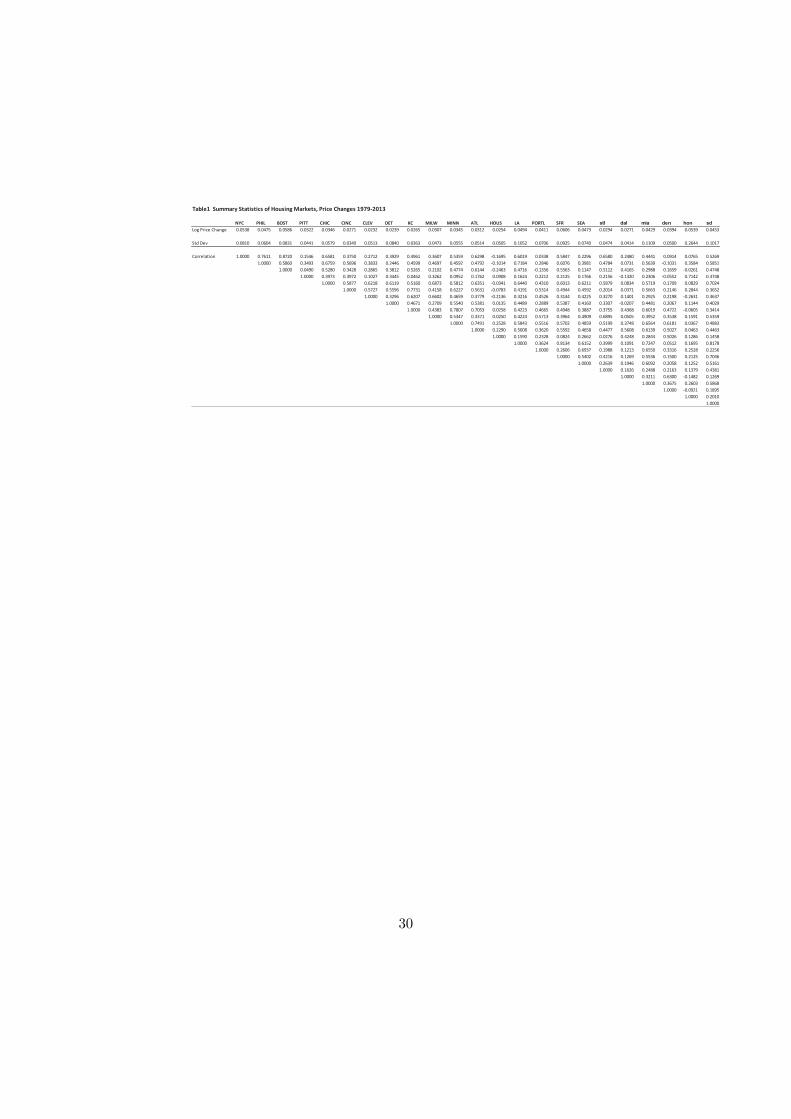
Table1 Summary Statistics of Housing Markets, Price Changes 1979-2013
NYC PHIL BOST PITT CHIC CINC CLEV DET KC MILW MINN ATL HOUS LA PORTL SFR SEA stl dal mia den hon sd
Log Price Change 0.0538 0.0475 0.0586 0.0322 0.0346 0.0271 0.0232 0.0239 0.0265 0.0307 0.0345 0.0312 0.0254 0.0494 0.0411 0.0606 0.0473 0.0294 0.0271 0.0429 0.0394 0.0539 0.0453
Std Dev 0.0810 0.0604 0.0831 0.0441 0.0579 0.0340 0.0513 0.0840 0.0363 0.0473 0.0555 0.0514 0.0505 0.1052 0.0706 0.0925 0.0740 0.0474 0.0414 0.1109 0.0500 0.2644 0.1017
Correlation 1.0000 0.7611 0.8720 0.1546 0.6581 0.3750 0.2712 0.3929 0.4961 0.3607 0.5359 0.6298 -0.1695 0.6019 0.0338 0.5847 0.2296 0.6580 0.2480 0.4441 0.0914 0.0765 0.5269
1.0000 0.5860 0.3493 0.6759 0.5696 0.3833 0.2446 0.4599 0.4697 0.4592 0.4792 -0.1014 0.7184 0.2846 0.6076 0.3981 0.4784 0.0731 0.5639 -0.1031 0.3584 0.5851
1.0000 0.0490 0.5280 0.3428 0.2865 0.3812 0.5265 0.2102 0.4774 0.6144 -0.2463 0.4716 -0.1356 0.5563 0.1147 0.5112 0.4165 0.2988 0.1659 -0.0261 0.4748
1.0000 0.3973 0.3972 0.1027 0.3445 0.0462 0.3262 0.0952 0.1762 0.0908 0.1624 0.2212 0.2125 0.1766 0.2156 -0.1320 0.2306 -0.0552 0.7142 0.3748
1.0000 0.5877 0.6218 0.6119 0.5160 0.6873 0.5812 0.6351 -0.0341 0.6440 0.4310 0.6013 0.6211 0.5879 0.0834 0.5719 0.1709 0.0829 0.7024
1.0000 0.5727 0.5596 0.7731 0.4158 0.6227 0.5631 -0.0783 0.4191 0.5314 0.4944 0.4592 0.2014 0.0371 0.5663 0.2146 0.2844 0.3652
1.0000 0.3296 0.6207 0.6602 0.4659 0.3779 -0.2136 0.3216 0.4526 0.3144 0.4225 0.3270 0.1401 0.2925 0.2198 -0.2631 0.3637
1.0000 0.4671 0.2709 0.5540 0.5381 0.0135 0.4489 0.2889 0.5387 0.4160 0.3307 -0.0207 0.4481 0.2067 0.1144 0.4029
1.0000 0.4383 0.7807 0.7053 0.0258 0.4223 0.4665 0.4948 0.3887 0.3755 0.4368 0.6019 0.4722 -0.0605 0.3414
1.0000 0.5347 0.3371 0.0250 0.4224 0.5713 0.3964 0.4909 0.6895 0.0505 0.3952 0.3538 0.1591 0.5359
1.0000 0.7491 0.2528 0.5843 0.5516 0.5702 0.4859 0.5199 0.3748 0.6564 0.6181 0.0367 0.4883
1.0000 0.2290 0.5008 0.3620 0.5592 0.4658 0.4477 0.5608 0.6139 0.5027 0.0463 0.4463
1.0000 0.1590 0.2328 0.0824 0.2662 0.0276 0.4248 0.2844 0.5026 0.1286 0.1458
1.0000 0.3624 0.8134 0.6152 0.3999 0.1091 0.7247 0.0512 0.1695 0.8178
1.0000 0.2606 0.6937 0.1988 0.1213 0.6550 0.3316 0.2528 0.2256
1.0000 0.5402 0.4216 0.1269 0.5536 0.1500 0.2125 0.7046
1.0000 0.2639 0.1946 0.6092 0.2058 0.1252 0.5161
1.0000 0.1626 0.2488 0.2163 0.1379 0.4381
1.0000 0.3211 0.6300 -0.1482 0.1269
1.0000 0.3675 0.2603 0.5868
1.0000 -0.0921 0.1895
1.0000 0.2010
1.0000
30
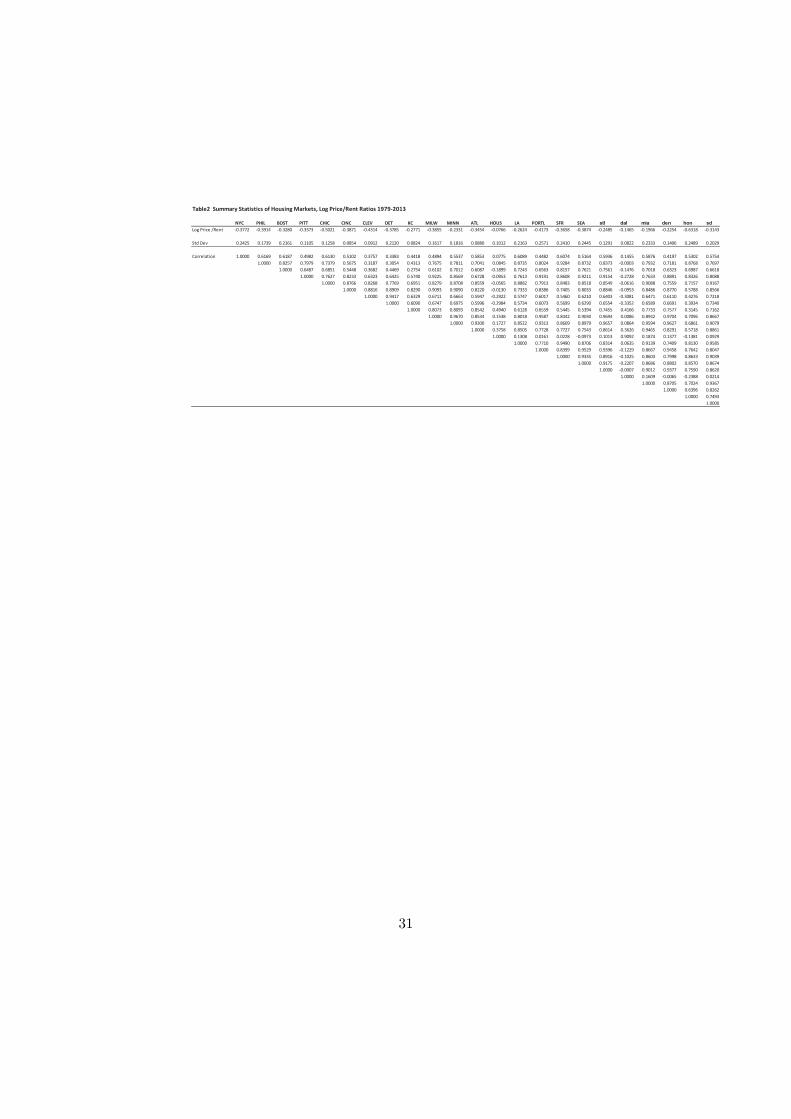
Table2 Summary Statistics of Housing Markets, Log Price/Rent Ratios 1979-2013
NYC PHIL BOST PITT CHIC CINC CLEV DET KC MILW MINN ATL HOUS LA PORTL SFR SEA stl dal mia den hon sd
Log Price /Rent -0.3772 -0.3914 -0.3280 -0.3373 -0.5021 -0.3871 -0.4314 -0.3785 -0.2771 -0.3855 -0.2331 -0.3454 -0.0766 -0.2624 -0.4173 -0.3658 -0.3874 -0.2485 -0.1465 -0.1966 -0.2254 -0.6318 -0.3143
Std Dev 0.2425 0.1739 0.2161 0.1105 0.1258 0.0854 0.0912 0.2120 0.0824 0.1617 0.1816 0.0880 0.1012 0.2163 0.2571 0.2410 0.2445 0.1291 0.0822 0.2333 0.1406 0.2489 0.2029
Correlation 1.0000 0.6169 0.6187 0.4982 0.6130 0.5102 0.3757 0.3383 0.4418 0.4894 0.5537 0.5853 0.0775 0.6089 0.4482 0.6074 0.5164 0.5936 0.1455 0.5876 0.4197 0.5302 0.5754
1.0000 0.8257 0.7979 0.7379 0.5675 0.3187 0.3054 0.4313 0.7675 0.7811 0.7041 0.0845 0.8735 0.8024 0.9284 0.8732 0.8373 -0.0003 0.7932 0.7181 0.8768 0.7697
1.0000 0.6487 0.6851 0.5448 0.3682 0.4469 0.2754 0.6102 0.7012 0.6087 -0.1899 0.7243 0.6563 0.8157 0.7621 0.7561 -0.1476 0.7018 0.6323 0.6987 0.6618
1.0000 0.7627 0.8233 0.6323 0.6425 0.5740 0.9225 0.8569 0.6728 -0.0953 0.7613 0.9191 0.8608 0.9211 0.9154 -0.2728 0.7633 0.8891 0.8326 0.8088
1.0000 0.8766 0.8268 0.7769 0.6951 0.8279 0.8708 0.8559 -0.0565 0.8882 0.7913 0.8483 0.8518 0.8549 -0.0616 0.9088 0.7559 0.7157 0.9167
1.0000 0.8816 0.8909 0.8290 0.9093 0.9090 0.8220 -0.0130 0.7333 0.8386 0.7405 0.8033 0.8846 -0.0953 0.8486 0.8770 0.5788 0.8566
1.0000 0.9417 0.6329 0.6711 0.6663 0.5947 -0.2922 0.5747 0.6017 0.5460 0.6210 0.6403 -0.3081 0.6471 0.6110 0.4276 0.7218
1.0000 0.6090 0.6747 0.6975 0.5996 -0.2984 0.5734 0.6073 0.5699 0.6290 0.6554 -0.3352 0.6589 0.6691 0.3934 0.7340
1.0000 0.8073 0.8093 0.8542 0.4940 0.6128 0.6559 0.5445 0.5394 0.7455 0.4166 0.7733 0.7577 0.3145 0.7162
1.0000 0.9670 0.8534 0.1538 0.8018 0.9587 0.8442 0.9030 0.9694 0.0086 0.8942 0.9704 0.7096 0.8667
1.0000 0.9300 0.1727 0.8522 0.9313 0.8609 0.8979 0.9657 0.0864 0.9594 0.9627 0.6861 0.9079
1.0000 0.3758 0.8505 0.7728 0.7727 0.7543 0.8614 0.3626 0.9465 0.8291 0.5718 0.8861
1.0000 0.1308 0.0161 0.0228 -0.0973 0.1013 0.9092 0.1874 0.1377 -0.1381 0.0929
1.0000 0.7710 0.9490 0.8706 0.8314 0.0635 0.9139 0.7409 0.8130 0.9585
1.0000 0.8399 0.9529 0.9396 -0.1229 0.8667 0.9458 0.7642 0.8047
1.0000 0.9335 0.8916 -0.1025 0.8603 0.7998 0.8633 0.9039
1.0000 0.9175 -0.2207 0.8686 0.8802 0.8570 0.8674
1.0000 -0.0007 0.9012 0.9377 0.7590 0.8620
1.0000 0.1609 -0.0065 -0.2388 0.0214
1.0000 0.8705 0.7024 0.9367
1.0000 0.6396 0.8262
1.0000 0.7493
1.0000
31
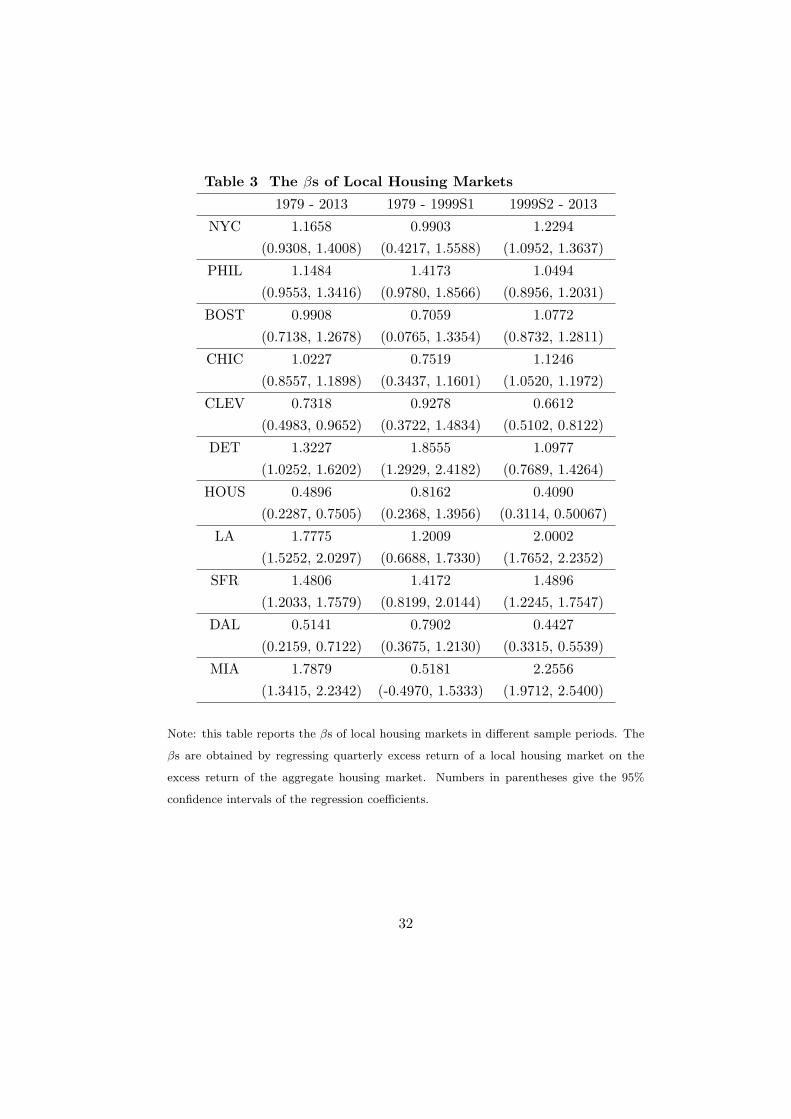
Table 3 The βs of Local Housing Markets
1979 - 2013 1979 - 1999S1 1999S2 - 2013
NYC 1.1658 0.9903 1.2294
(0.9308, 1.4008) (0.4217, 1.5588) (1.0952, 1.3637)
PHIL 1.1484 1.4173 1.0494
(0.9553, 1.3416) (0.9780, 1.8566) (0.8956, 1.2031)
BOST 0.9908 0.7059 1.0772
(0.7138, 1.2678) (0.0765, 1.3354) (0.8732, 1.2811)
CHIC 1.0227 0.7519 1.1246
(0.8557, 1.1898) (0.3437, 1.1601) (1.0520, 1.1972)
CLEV 0.7318 0.9278 0.6612
(0.4983, 0.9652) (0.3722, 1.4834) (0.5102, 0.8122)
DET 1.3227 1.8555 1.0977
(1.0252, 1.6202) (1.2929, 2.4182) (0.7689, 1.4264)
HOUS 0.4896 0.8162 0.4090
(0.2287, 0.7505) (0.2368, 1.3956) (0.3114, 0.50067)
LA 1.7775 1.2009 2.0002
(1.5252, 2.0297) (0.6688, 1.7330) (1.7652, 2.2352)
SFR 1.4806 1.4172 1.4896
(1.2033, 1.7579) (0.8199, 2.0144) (1.2245, 1.7547)
DAL 0.5141 0.7902 0.4427
(0.2159, 0.7122) (0.3675, 1.2130) (0.3315, 0.5539)
MIA 1.7879 0.5181 2.2556
(1.3415, 2.2342) (-0.4970, 1.5333) (1.9712, 2.5400)
Note: this table reports the βs of local housing markets in different sample periods. The
βs are obtained by regressing quarterly excess return of a local housing market on the
excess return of the aggregate housing market. Numbers in parentheses give the 95%
confidence intervals of the regression coefficients.
32
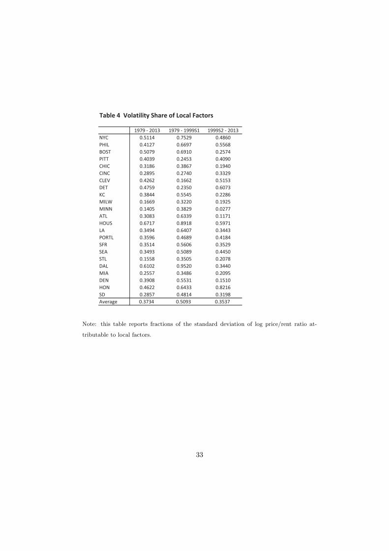
Table 4 Volatility Share of Local Factors
1979 - 2013 1979 - 1999S1 1999S2 - 2013
NYC 0.5114 0.7529 0.4860
PHIL 0.4127 0.6697 0.5568
BOST 0.5079 0.6910 0.2574
PITT 0.4039 0.2453 0.4090
CHIC 0.3186 0.3867 0.1940
CINC 0.2895 0.2740 0.3329
CLEV 0.4262 0.1662 0.5153
DET 0.4759 0.2350 0.6073
KC 0.3844 0.5545 0.2286
MILW 0.1669 0.3220 0.1925
MINN 0.1405 0.3829 0.0277
ATL 0.3083 0.6339 0.1171
HOUS 0.6717 0.8918 0.5971
LA 0.3494 0.6407 0.3443
PORTL 0.3596 0.4689 0.4184
SFR 0.3514 0.5606 0.3529
SEA 0.3493 0.5089 0.4450
STL 0.1558 0.3505 0.2078
DAL 0.6102 0.9520 0.3440
MIA 0.2557 0.3486 0.2095
DEN 0.3908 0.5531 0.1510
HON 0.4622 0.6433 0.8216
SD 0.2857 0.4814 0.3198
Average 0.3734 0.5093 0.3537
Note: this table reports fractions of the standard deviation of log price/rent ratio at-
tributable to local factors.
33
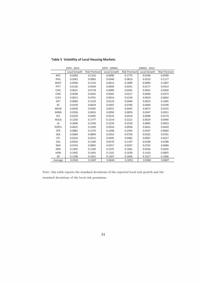
Table 5 Volatility of Local Housing Markets
1979 - 2013 1979 - 1999S1 1999S2 - 2013
Local Growth Risk Premium Local Growth Risk Premium Local Growth Risk Premium
NYC 0.0283 0.1316 0.0090 0.1773 0.0196 0.0599
PHIL 0.0363 0.0963 0.0340 0.0819 0.0310 0.1177
BOST 0.0560 0.1516 0.0612 0.1899 0.0894 0.1007
PITT 0.0126 0.0504 0.0049 0.0241 0.0177 0.0314
CHIC 0.0021 0.0778 0.0009 0.0365 0.0031 0.0304
CINC 0.0038 0.0343 0.0045 0.0217 0.0040 0.0373
CLEV 0.0012 0.0791 0.0014 0.0149 0.0019 0.0662
DET 0.0069 0.1529 0.0124 0.0446 0.0023 0.1845
KC 0.0149 0.0629 0.0307 0.0766 0.0044 0.0190
MILW 0.0030 0.0305 0.0031 0.0445 0.0072 0.0225
MINN 0.0336 0.0453 0.0950 0.0876 0.0347 0.0351
ATL 0.0259 0.0495 0.0233 0.0410 0.0096 0.0174
HOUS 0.1203 0.1777 0.1519 0.2212 0.0019 0.0440
LA 0.2000 0.2190 0.2234 0.2530 0.0895 0.0923
PORTL 0.0625 0.1030 0.0554 0.0958 0.0631 0.0459
SFR 0.0882 0.1570 0.1698 0.2454 0.0337 0.0660
SEA 0.0384 0.0894 0.0353 0.0756 0.0325 0.0701
STL 0.0243 0.0315 0.0445 0.0482 0.0007 0.0227
DAL 0.0416 0.1160 0.0570 0.1197 0.0189 0.0298
MIA 0.0743 0.0892 0.0257 0.0297 0.0763 0.0684
DEN 0.1402 0.1330 0.1975 0.1681 0.0426 0.0435
HON 0.1092 0.1643 0.1101 0.1639 0.1410 0.0855
SD 0.1298 0.1652 0.1307 0.1606 0.1017 0.1066
Average 0.0545 0.1047 0.0644 0.1053 0.0360 0.0607
Note: this table reports the standard deviations of the expected local rent growth and the
standard deviations of the local risk premiums.
34
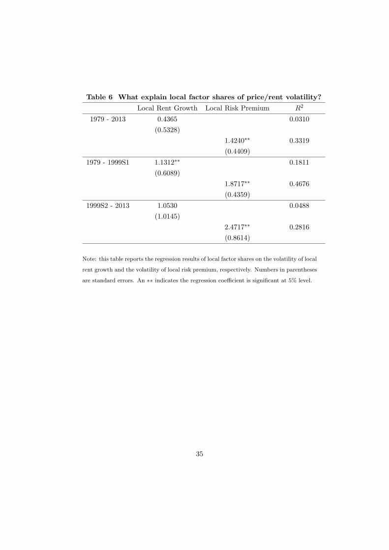
Table 6 What explain local factor shares of price/rent volatility?
Local Rent Growth Local Risk Premium R2
1979 - 2013 0.4365 0.0310
(0.5328)
1.4240∗∗ 0.3319
(0.4409)
1979 - 1999S1 1.1312∗∗ 0.1811
(0.6089)
1.8717∗∗ 0.4676
(0.4359)
1999S2 - 2013 1.0530 0.0488
(1.0145)
2.4717∗∗ 0.2816
(0.8614)
Note: this table reports the regression results of local factor shares on the volatility of local
rent growth and the volatility of local risk premium, respectively. Numbers in parentheses
are standard errors. An ∗∗ indicates the regression coefficient is significant at 5% level.
35
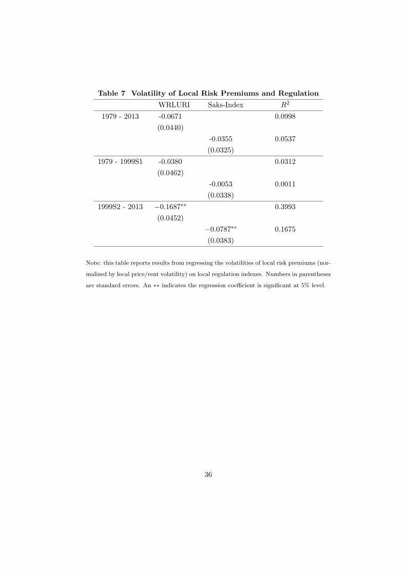
Table 7 Volatility of Local Risk Premiums and Regulation
WRLURI Saks-Index R2
1979 - 2013 -0.0671 0.0998
(0.0440)
-0.0355 0.0537
(0.0325)
1979 - 1999S1 -0.0380 0.0312
(0.0462)
-0.0053 0.0011
(0.0338)
1999S2 - 2013 −0.1687∗∗ 0.3993
(0.0452)
−0.0787∗∗ 0.1675
(0.0383)
Note: this table reports results from regressing the volatilities of local risk premiums (nor-
malized by local price/rent volatility) on local regulation indexes. Numbers in parentheses
are standard errors. An ∗∗ indicates the regression coefficient is significant at 5% level.
36
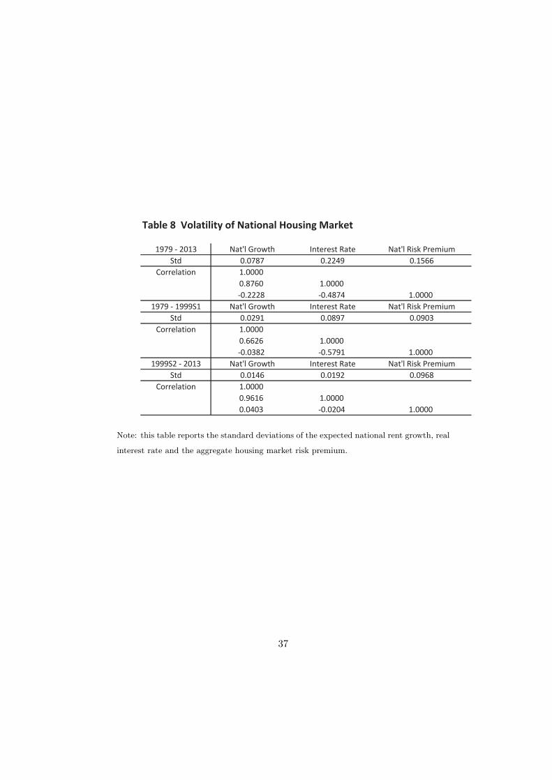
Table 8 Volatility of National Housing Market
1979 - 2013 Nat'l Growth Interest Rate Nat'l Risk Premium
Std 0.0787 0.2249 0.1566
Correlation 1.0000
0.8760 1.0000
-0.2228 -0.4874 1.0000
1979 - 1999S1 Nat'l Growth Interest Rate Nat'l Risk Premium
Std 0.0291 0.0897 0.0903
Correlation 1.0000
0.6626 1.0000
-0.0382 -0.5791 1.0000
1999S2 - 2013 Nat'l Growth Interest Rate Nat'l Risk Premium
Std 0.0146 0.0192 0.0968
Correlation 1.0000
0.9616 1.0000
0.0403 -0.0204 1.0000
Note: this table reports the standard deviations of the expected national rent growth, real
interest rate and the aggregate housing market risk premium.
37
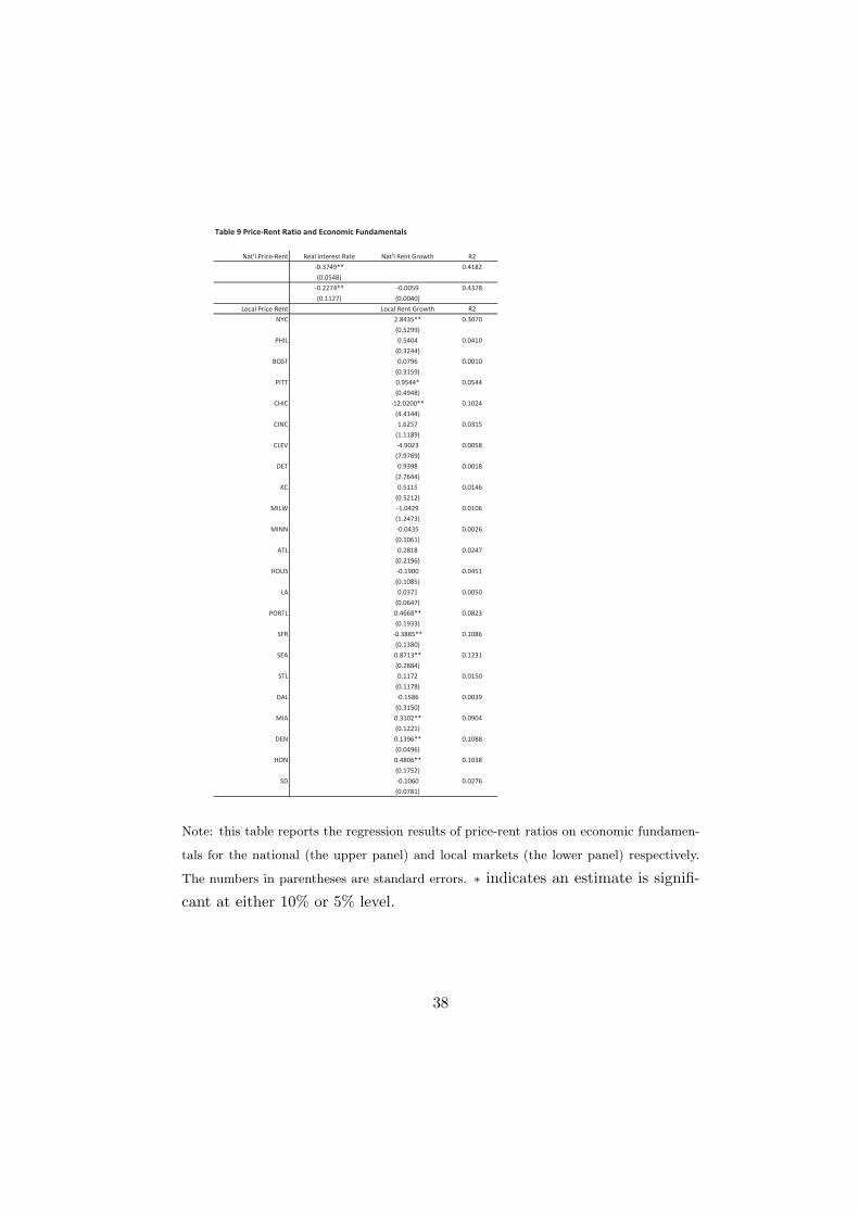
Table 9 Price-Rent Ratio and Economic Fundamentals
Nat'l Price-Rent Real Interest Rate Nat'l Rent Growth R2
-0.3749** 0.4182
(0.0548)
-0.2274** -0.0059 0.4378
(0.1127) (0.0040)
Local Price-Rent Local Rent Growth R2
NYC 2.8435** 0.3070
(0.5299)
PHIL 0.5404 0.0410
(0.3244)
BOST 0.0796 0.0010
(0.3159)
PITT 0.9544* 0.0544
(0.4948)
CHIC -12.0200** 0.1024
(4.4144)
CINC 1.6257 0.0315
(1.1189)
CLEV -4.9023 0.0058
(7.9769)
DET 0.9398 0.0018
(2.7644)
KC 0.5115 0.0146
(0.5212)
MILW -1.0429 0.0106
(1.2473)
MINN -0.0435 0.0026
(0.1061)
ATL 0.2818 0.0247
(0.2196)
HOUS -0.1900 0.0451
(0.1085)
LA 0.0371 0.0050
(0.0647)
PORTL 0.4668** 0.0823
(0.1933)
SFR -0.3885** 0.1086
(0.1380)
SEA 0.8713** 0.1231
(0.2884)
STL 0.1172 0.0150
(0.1178)
DAL -0.1586 0.0039
(0.3150)
MIA 0.3102** 0.0904
(0.1221)
DEN 0.1396** 0.1088
(0.0496)
HON 0.4806** 0.1038
(0.1752)
SD -0.1060 0.0276
(0.0781)
Note: this table reports the regression results of price-rent ratios on economic fundamen-
tals for the national (the upper panel) and local markets (the lower panel) respectively.
The numbers in parentheses are standard errors. ∗ indicates an estimate is signifi-
cant at either 10% or 5% level.
38
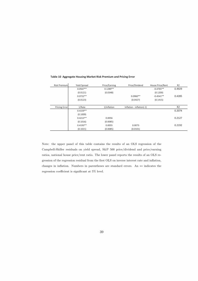
Table 10 Aggregate Housing Market Risk Premium and Pricing Error
Risk Premium Yield Spread Price/Earning Price/Dividend House Price/Rent R2
0.0567** 0.1289** -0.4765** 0.4929
(0.0121) (0.0348) (0.1200)
0.0722** 0.0960** -0.4541** 0.4285
(0.0123) (0.0427) (0.1415)
Pricing Error 1/Rate 1/inflation Inflation - inflation(-1) R2
0.4159** 0.2074
(0.1009)
0.4213** 0.0056 0.2127
(0.1016) (0.0085)
0.4193** 0.0055 0.0073 0.2192
(0.1021) (0.0085) (0.0101)
Note: the upper panel of this table contains the results of an OLS regression of the
Campbell-Shiller residuals on yield spread, S&P 500 price/dividend and price/earning
ratios, national house price/rent ratio. The lower panel reports the results of an OLS re-
gression of the regression residual from the first OLS on inverse interest rate and inflation,
changes in inflation. Numbers in parentheses are standard errors. An ∗∗ indicates the
regression coefficient is significant at 5% level.
39
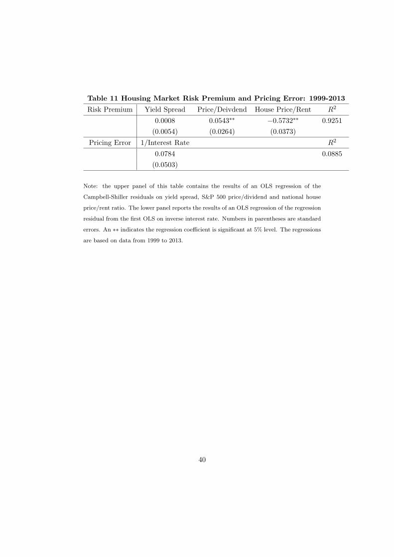
Table 11 Housing Market Risk Premium and Pricing Error: 1999-2013
Risk Premium Yield Spread Price/Deivdend House Price/Rent R2
0.0008 0.0543∗∗ −0.5732∗∗ 0.9251
(0.0054) (0.0264) (0.0373)
Pricing Error 1/Interest Rate R2
0.0784 0.0885
(0.0503)
Note: the upper panel of this table contains the results of an OLS regression of the
Campbell-Shiller residuals on yield spread, S&P 500 price/dividend and national house
price/rent ratio. The lower panel reports the results of an OLS regression of the regression
residual from the first OLS on inverse interest rate. Numbers in parentheses are standard
errors. An ∗∗ indicates the regression coefficient is significant at 5% level. The regressions
are based on data from 1999 to 2013.
40
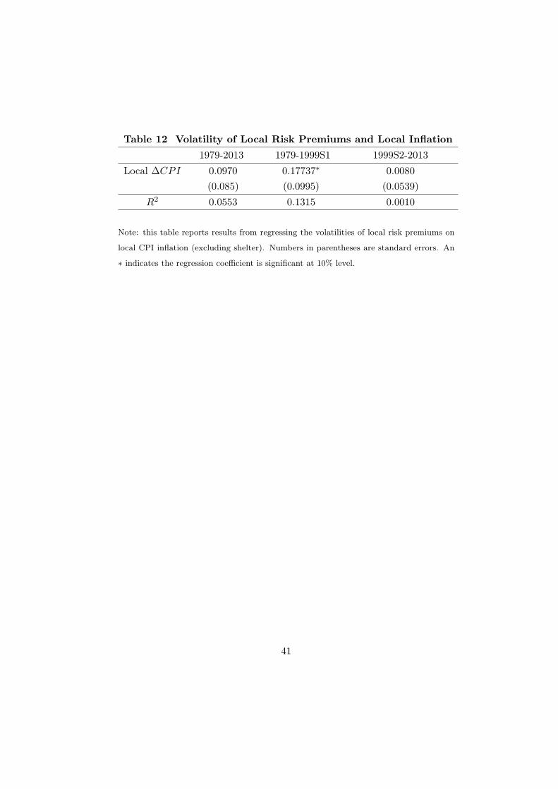
Table 12 Volatility of Local Risk Premiums and Local Inflation
1979-2013 1979-1999S1 1999S2-2013
Local ∆CPI 0.0970 0.17737∗ 0.0080
(0.085) (0.0995) (0.0539)
R2 0.0553 0.1315 0.0010
Note: this table reports results from regressing the volatilities of local risk premiums on
local CPI inflation (excluding shelter). Numbers in parentheses are standard errors. An
∗ indicates the regression coefficient is significant at 10% level.
41
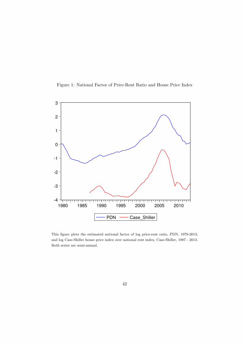
Figure 1: National Factor of Price-Rent Ratio and House Price Index
-4
-3
-2
-1
0
1
2
3
1980 1985 1990 1995 2000 2005 2010
PDN Case_Shiller
This figure plots the estimated national factor of log price-rent ratio, PDN, 1979-2013,
and log Case-Shiller house price index over national rent index, Case-Shiller, 1987 - 2013.
Both series are semi-annual.
42
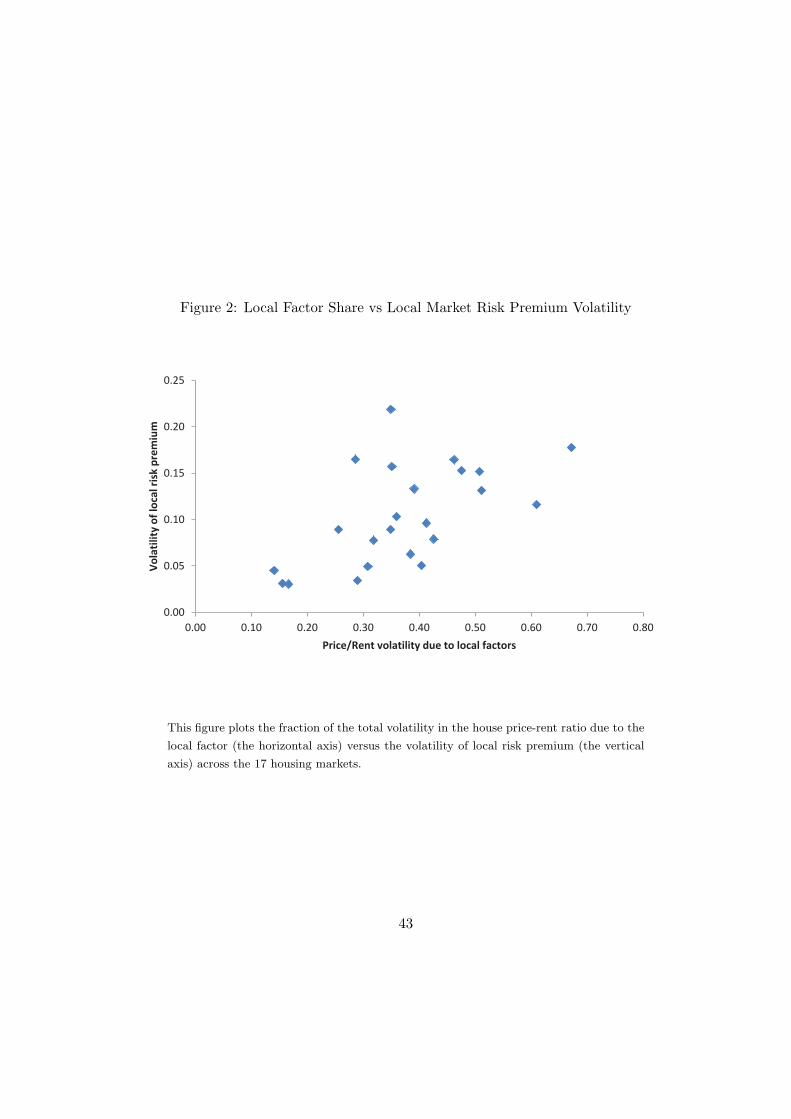
Figure 2: Local Factor Share vs Local Market Risk Premium Volatility
0.00
0.05
0.10
0.15
0.20
0.25
0.00 0.10 0.20 0.30 0.40 0.50 0.60 0.70 0.80
Vo
lati
lity
of
loca
l ri
sk p
rem
ium
Price/Rent volatility due to local factors
This figure plots the fraction of the total volatility in the house price-rent ratio due to the
local factor (the horizontal axis) versus the volatility of local risk premium (the vertical
axis) across the 17 housing markets.
43
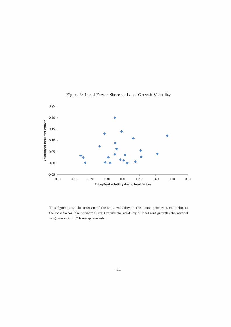
Figure 3: Local Factor Share vs Local Growth Volatility
-0.05
0.00
0.05
0.10
0.15
0.20
0.25
0.00 0.10 0.20 0.30 0.40 0.50 0.60 0.70 0.80
Vo
lati
lity
of
loca
l re
nt
gro
wth
Price/Rent volatility due to local factors
This figure plots the fraction of the total volatility in the house price-rent ratio due to
the local factor (the horizontal axis) versus the volatility of local rent growth (the vertical
axis) across the 17 housing markets.
44
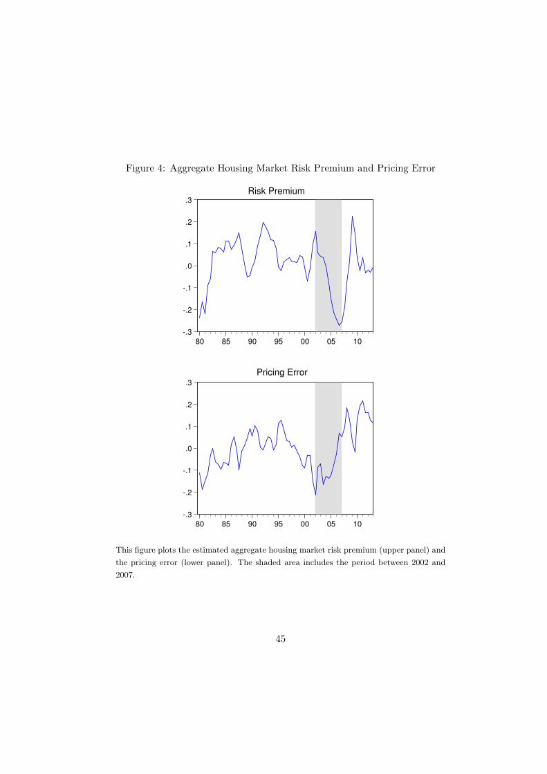
Figure 4: Aggregate Housing Market Risk Premium and Pricing Error
-.3
-.2
-.1
.0
.1
.2
.3
80 85 90 95 00 05 10
Risk Premium
-.3
-.2
-.1
.0
.1
.2
.3
80 85 90 95 00 05 10
Pricing Error
This figure plots the estimated aggregate housing market risk premium (upper panel) and
the pricing error (lower panel). The shaded area includes the period between 2002 and
2007.
45