Understanding How Image Quality Affects DeepNeural Networks

Samuel Dodge and Lina KaramArizona State University

sfdodge@asu.edu, karam@asu.edu

Abstract—Image quality is an important practical challengethat is often overlooked in the design of machine vision systems.Commonly, machine vision systems are trained and tested onhigh quality image datasets, yet in practical applications theinput images can not be assumed to be of high quality. Recently,deep neural networks have obtained state-of-the-art performanceon many machine vision tasks. In this paper we provide anevaluation of 4 state-of-the-art deep neural network models forimage classification under quality distortions. We consider fivetypes of quality distortions: blur, noise, contrast, JPEG, andJPEG2000 compression. We show that the existing networks aresusceptible to these quality distortions, particularly to blur andnoise. These results enable future work in developing deep neuralnetworks that are more invariant to quality distortions.

I. INTRODUCTION

Visual quality evaluation has traditionally been focusedon the perception of quality from the perspective of humansubjects. However, with growing applications of computervision, it is also important to characterize the effect of imagequality on computer vision systems. These two notions ofimage quality may not be directly comparable as the computermay be fooled by images that are perceived by humans to beidentical [1], or in some cases the computer can recognizeimages that are indistinguishable from noise by a humanobserver [2]. Thus, it is important to separately consider howimage quality can affect computer vision applications.

In computer vision, recent techniques based on deep neuralnetworks (DNN) have begun to achieve state-of-the-art resultsin many problem domains [3]. Of particular interest to DNNmodels is image classification performance on large scaledatasets with millions of images and thousands of categories.These problem domains were previously thought to be ex-tremely difficult, but DNNs have achieved very impressiveresults. For example, in the ILSVRC 2010 challenge, theAlexNet DNN[4] achieved the best result with nearly 9%better classification accuracy than the second best result basedon hand-crafted features.

Despite their impressive performance, deep networks havebeen shown to be susceptible to adversarial samples [1].Adversarial samples are generated by adding worst case noiseto the image such that the classification prediction is incorrectwith a high confidence. This worst case noise is imperceptibleto human observers. The noise is carefully chosen using eitheran optimization algorithm [6] or by exploiting linear propertiesof the network [1]. Adversarial samples present an interestingproblem, however in practice such carefully chosen noise isunlikely to be encountered.

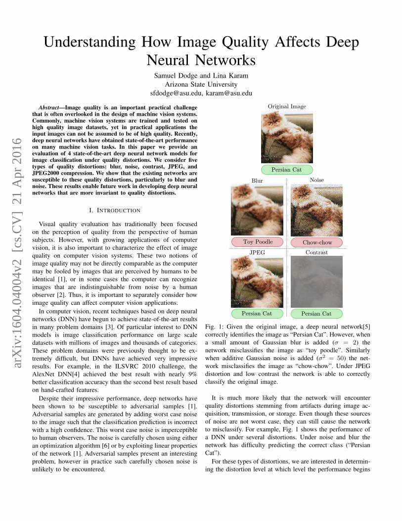
Toy Poodle

Blur

Chow-chow

Noise

Persian Cat

JPEG

Persian Cat

Contrast

Persian Cat

Original Image

Fig. 1: Given the original image, a deep neural network[5]correctly identifies the image as “Persian Cat”. However, whena small amount of Gaussian blur is added (σ = 2) thenetwork misclassifies the image as “toy poodle”. Similarlywhen additive Gaussian noise is added (σ2 = 50) the net-work misclassifies the image as “chow-chow”. Under JPEGdistortion and low contrast the network is able to correctlyclassify the original image.

It is much more likely that the network will encounterquality distortions stemming from artifacts during image ac-quisition, transmission, or storage. Even though these sourcesof noise are not worst case, they can still cause the networkto misclassify. For example, Fig. 1 shows the performance ofa DNN under several distortions. Under noise and blur thenetwork has difficulty predicting the correct class (“PersianCat”).

For these types of distortions, we are interested in determin-ing the distortion level at which level the performance begins

arX

iv:1

604.

0400

4v2

[cs

.CV

] 2

1 A

pr 2

016

to decrease. Also, it is interesting to investigate whether thestructure of the network significantly affects the ability to beinvariant to quality distortions. This will give insight as towhat architectures would be useful for building networks thatare more invariant to these distortions.

A. Related Works

For many applications in computer vision it is assumed thatthe input images are of relatively high quality. However, incertain application domains such as surveillance, image qualityis an important consideration. Additionally, with the adventof many computer vision applications on cellular phones, therequirement of high quality images may need to be relaxed.

In surveillance applications, face recognition in low qualityimages is an important capability. There are many works thatattempt to recognize low-resolution faces [7], [8]. Besideslow-resolution, other image quality distortions may affectperformance. Karam and Zhu [9] present a face recognitiondataset that considers five different types of quality distortions.They however do not evaluate the performance of any modelson this new dataset. Tao et al. [10] present an approach basedon sparse representations that achieves good performance onthis dataset.

For hand-written digit recognition, Basu et al. [11] presentthe n-MNIST database, which is a modification of the bench-mark MNIST dataset. n-MNIST adds Gaussian noise, motionblur, and reduced contrast to the original images. Additionally,the authors in [11] propose a modification of deep beliefnetworks to achieve greater accuracy on this dataset.

Ullman et al. [12] consider deep neural network perfor-mance on low resolution crops of an image. They find minimalrecognizable configurations of images (MIRCs) which are thesmallest crops for which human observers can still predict thecorrect class. MIRCs are discovered by repeatedly croppingthe input image and asking human observers if they can stillrecognize the cropped image. The MIRC regions are blurrybecause in general they represent very small regions. Theauthors test deep networks on the MIRC regions and showthat they cannot match human performance. By contrast, inthis paper we consider blurring the entire image rather thanselecting a small region of the image, in addition to other typesof distortions that occur in practical applications.

In this paper, we present the first large scale evaluation ofdeep networks on natural images under different types anddifferent levels of image quality distortions. In contrast to[11], [9], we use the ILSVRC 2012 dataset (ImageNet) [13]which consists of 1000 object classes. The original imagesfrom this database are relatively high quality. We augment thisdataset by introducing several distortions and then evaluate theperformance of state-of-the-art deep neural networks on thesedistorted images.

II. BACKGROUND

Here we provide a brief overview of deep neural networks.A more detailed overview can be found in [14]. Deep neuralnetworks are inspired by biological neural networks. That is,

they are a collection of small, simple elements called neurons.In general, a deep network consists of layers of neurons whereeach neuron computes the following activation function:

f(x) = φ(wTx+ b) (1)

where x is the input to the neuron, w is a weight vector,b is a bias term and φ is a nonlinearity function. Eachneuron receives potentially many inputs, and outputs a singlenumber. The nonlinearity is important because it allows layersof neurons to learn non-linear functions. In these layeredstructures, the output of one layer of units becomes the inputsto the next layer of units. The networks considered in thispaper use Rectified Linear Units [15] as the nonlinearityfunction.

For image recognition problems, the input to the networkis the image itself (usually normalized). However, if a singleneuron is to receive inputs from the entire image, the memoryand computational requirements quickly become prohibitive.To mitigate this problem weight sharing is used. Rather thaneach neuron using a separate weight vector w, this vector isshared between neurons. The weight vector connects to nearbyneurons from the previous layer within a pre-defined regionknown as a receptive field. In practice, this process is identicalto convolutional filtering with the filter represented by theweights. Layers with convolutional shared weights are calledconvolutional layers. Layers without the convolutional sharedweights are called fully connected layers.

In addition to convolutional layers, networks often incor-porate a max pooling stage. This stage serves two purposes:to improve robustness to noise in filter responses, and toincrease the size of the receptive field in the next layer withoutincreasing the size of the filter. This operation considers awindow (often 2x2 or 3x3 pixels) and takes the maximumneuron response in each window across the input.

The last stage of the network is typically a softmax layer.The softmax normalizes the responses of the units such thatthey sum to one. In this way the output layer becomes aprobability distribution with each neuron corresponding to theprobability (or confidence) of the network for a particularclass.

The network parameters (w and b for each unit) are trainedusing a large set of input images. First the output of thenetwork is computed for a given set of images. This outputis compared to the known class labels and a cost functionindicates how closely the predictions match the ground truth.The gradient of this cost function can be computed, and bypropagating this gradient backwards through the network, thegradient of each neuron is computed. With the gradient, anynumber of optimization techniques based on gradient descentcan be used to optimize the weights. This general frameworkis called the backpropagation algorithm [16].

III. EXPERIMENTAL SETUP

A. Deep Networks

In this paper we consider four representative neural net-works. Table I summarizes the considered models. Although

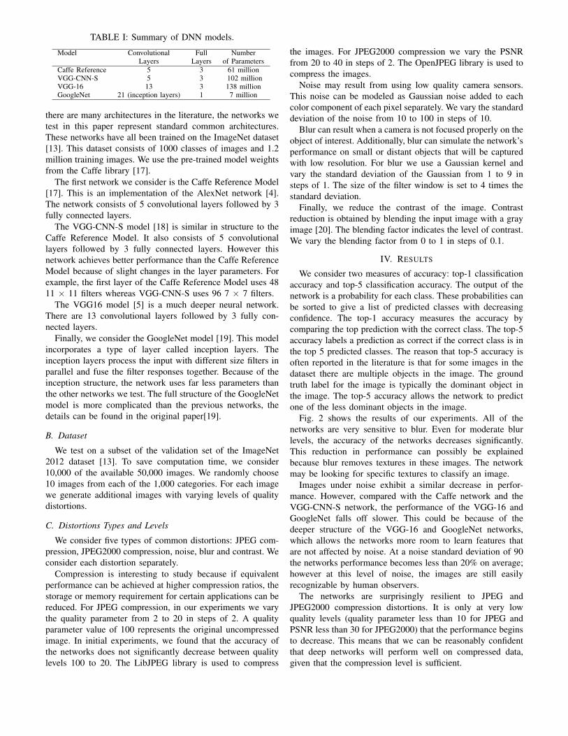
TABLE I: Summary of DNN models.

Model Convolutional Full NumberLayers Layers of Parameters

Caffe Reference 5 3 61 millionVGG-CNN-S 5 3 102 millionVGG-16 13 3 138 millionGoogleNet 21 (inception layers) 1 7 million

there are many architectures in the literature, the networks wetest in this paper represent standard common architectures.These networks have all been trained on the ImageNet dataset[13]. This dataset consists of 1000 classes of images and 1.2million training images. We use the pre-trained model weightsfrom the Caffe library [17].

The first network we consider is the Caffe Reference Model[17]. This is an implementation of the AlexNet network [4].The network consists of 5 convolutional layers followed by 3fully connected layers.

The VGG-CNN-S model [18] is similar in structure to theCaffe Reference Model. It also consists of 5 convolutionallayers followed by 3 fully connected layers. However thisnetwork achieves better performance than the Caffe ReferenceModel because of slight changes in the layer parameters. Forexample, the first layer of the Caffe Reference Model uses 4811 × 11 filters whereas VGG-CNN-S uses 96 7 × 7 filters.

The VGG16 model [5] is a much deeper neural network.There are 13 convolutional layers followed by 3 fully con-nected layers.

Finally, we consider the GoogleNet model [19]. This modelincorporates a type of layer called inception layers. Theinception layers process the input with different size filters inparallel and fuse the filter responses together. Because of theinception structure, the network uses far less parameters thanthe other networks we test. The full structure of the GoogleNetmodel is more complicated than the previous networks, thedetails can be found in the original paper[19].

B. Dataset

We test on a subset of the validation set of the ImageNet2012 dataset [13]. To save computation time, we consider10,000 of the available 50,000 images. We randomly choose10 images from each of the 1,000 categories. For each imagewe generate additional images with varying levels of qualitydistortions.

C. Distortions Types and Levels

We consider five types of common distortions: JPEG com-pression, JPEG2000 compression, noise, blur and contrast. Weconsider each distortion separately.

Compression is interesting to study because if equivalentperformance can be achieved at higher compression ratios, thestorage or memory requirement for certain applications can bereduced. For JPEG compression, in our experiments we varythe quality parameter from 2 to 20 in steps of 2. A qualityparameter value of 100 represents the original uncompressedimage. In initial experiments, we found that the accuracy ofthe networks does not significantly decrease between qualitylevels 100 to 20. The LibJPEG library is used to compress

the images. For JPEG2000 compression we vary the PSNRfrom 20 to 40 in steps of 2. The OpenJPEG library is used tocompress the images.

Noise may result from using low quality camera sensors.This noise can be modeled as Gaussian noise added to eachcolor component of each pixel separately. We vary the standarddeviation of the noise from 10 to 100 in steps of 10.

Blur can result when a camera is not focused properly on theobject of interest. Additionally, blur can simulate the network’sperformance on small or distant objects that will be capturedwith low resolution. For blur we use a Gaussian kernel andvary the standard deviation of the Gaussian from 1 to 9 insteps of 1. The size of the filter window is set to 4 times thestandard deviation.

Finally, we reduce the contrast of the image. Contrastreduction is obtained by blending the input image with a grayimage [20]. The blending factor indicates the level of contrast.We vary the blending factor from 0 to 1 in steps of 0.1.

IV. RESULTS

We consider two measures of accuracy: top-1 classificationaccuracy and top-5 classification accuracy. The output of thenetwork is a probability for each class. These probabilities canbe sorted to give a list of predicted classes with decreasingconfidence. The top-1 accuracy measures the accuracy bycomparing the top prediction with the correct class. The top-5accuracy labels a prediction as correct if the correct class is inthe top 5 predicted classes. The reason that top-5 accuracy isoften reported in the literature is that for some images in thedataset there are multiple objects in the image. The groundtruth label for the image is typically the dominant object inthe image. The top-5 accuracy allows the network to predictone of the less dominant objects in the image.

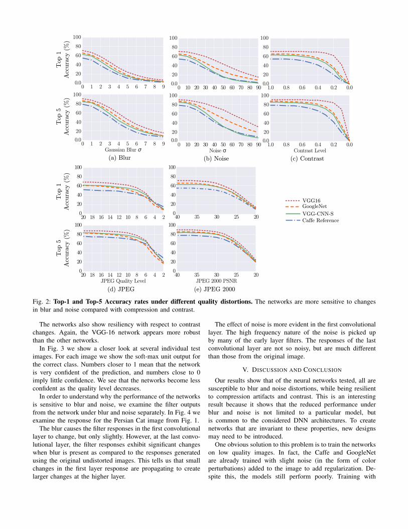
Fig. 2 shows the results of our experiments. All of thenetworks are very sensitive to blur. Even for moderate blurlevels, the accuracy of the networks decreases significantly.This reduction in performance can possibly be explainedbecause blur removes textures in these images. The networkmay be looking for specific textures to classify an image.

Images under noise exhibit a similar decrease in perfor-mance. However, compared with the Caffe network and theVGG-CNN-S network, the performance of the VGG-16 andGoogleNet falls off slower. This could be because of thedeeper structure of the VGG-16 and GoogleNet networks,which allows the networks more room to learn features thatare not affected by noise. At a noise standard deviation of 90the networks performance becomes less than 20% on average;however at this level of noise, the images are still easilyrecognizable by human observers.

The networks are surprisingly resilient to JPEG andJPEG2000 compression distortions. It is only at very lowquality levels (quality parameter less than 10 for JPEG andPSNR less than 30 for JPEG2000) that the performance beginsto decrease. This means that we can be reasonably confidentthat deep networks will perform well on compressed data,given that the compression level is sufficient.

(a) Blur

(d) JPEG (e) JPEG 2000

VGG16

VGG-CNN-S

Caffe Reference

GoogleNet

Top 1

Acc

ura

cy (

%)

Top 5

Acc

ura

cy (

%)

Top 1

Acc

ura

cy (

%)

Top 5

Acc

ura

cy (

%)

0 1 2 3 4 5 6 7 8 90.0

0.2

0.4

0.6

0.8

1.0

0 1 2 3 4 5 6 7 8 9Gaussian Blur σ

0.0

0.2

0.4

0.6

0.8

1.0

20

40

60

80

100

20

40

60

80

100

(c) Contrast

0.00.20.40.60.81.00.0

0.2

0.4

0.6

0.8

1.0

0.00.20.40.60.81.0Contrast Level

0.0

0.2

0.4

0.6

0.8

1.0

20

40

60

80

100

20

40

60

80

100

(b) Noise

0 10 20 30 40 50 60 70 80 900.0

0.2

0.4

0.6

0.8

1.0

0 10 20 30 40 50 60 70 80 90Noise σ

20

40

60

80

100

20

40

60

80

100

0.0

2025303540JPEG 2000 PSNR

0

20

40

60

80

100

20253035400

20

40

60

80

100

2468101214161820JPEG Quality Level

0

20

40

60

80

100

24681012141618200

20

40

60

80

100

Fig. 2: Top-1 and Top-5 Accuracy rates under different quality distortions. The networks are more sensitive to changesin blur and noise compared with compression and contrast.

The networks also show resiliency with respect to contrastchanges. Again, the VGG-16 network appears more robustthan the other networks.

In Fig. 3 we show a closer look at several individual testimages. For each image we show the soft-max unit output forthe correct class. Numbers closer to 1 mean that the networkis very confident of the prediction, and numbers close to 0imply little confidence. We see that the networks become lessconfident as the quality level decreases.

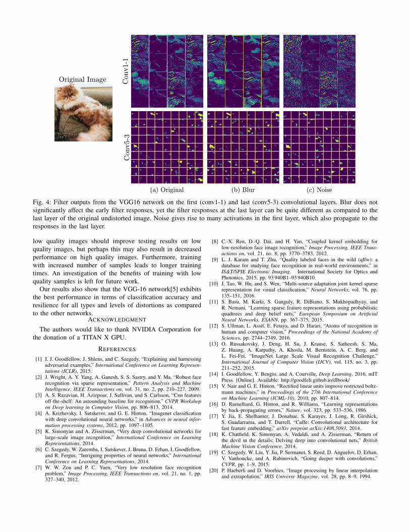
In order to understand why the performance of the networksis sensitive to blur and noise, we examine the filter outputsfrom the network under blur and noise separately. In Fig. 4 weexamine the response for the Persian Cat image from Fig. 1.

The blur causes the filter responses in the first convolutionallayer to change, but only slightly. However, at the last convo-lutional layer, the filter responses exhibit significant changeswhen blur is present as compared to the responses generatedusing the original undistorted images. This tells us that smallchanges in the first layer response are propagating to createlarger changes at the higher layer.

The effect of noise is more evident in the first convolutionallayer. The high frequency nature of the noise is picked upby many of the early layer filters. The responses of the lastconvolutional layer are not so noisy, but are much differentthan those from the original image.

V. DISCUSSION AND CONCLUSION

Our results show that of the neural networks tested, all aresusceptible to blur and noise distortions, while being resilientto compression artifacts and contrast. This is an interestingresult because it shows that the reduced performance underblur and noise is not limited to a particular model, butis common to the considered DNN architectures. To createnetworks that are invariant to these properties, new designsmay need to be introduced.

One obvious solution to this problem is to train the networkson low quality images. In fact, the Caffe and GoogleNetare already trained with slight noise (in the form of colorperturbations) added to the image to add regularization. De-spite this, the models still perform poorly. Training with

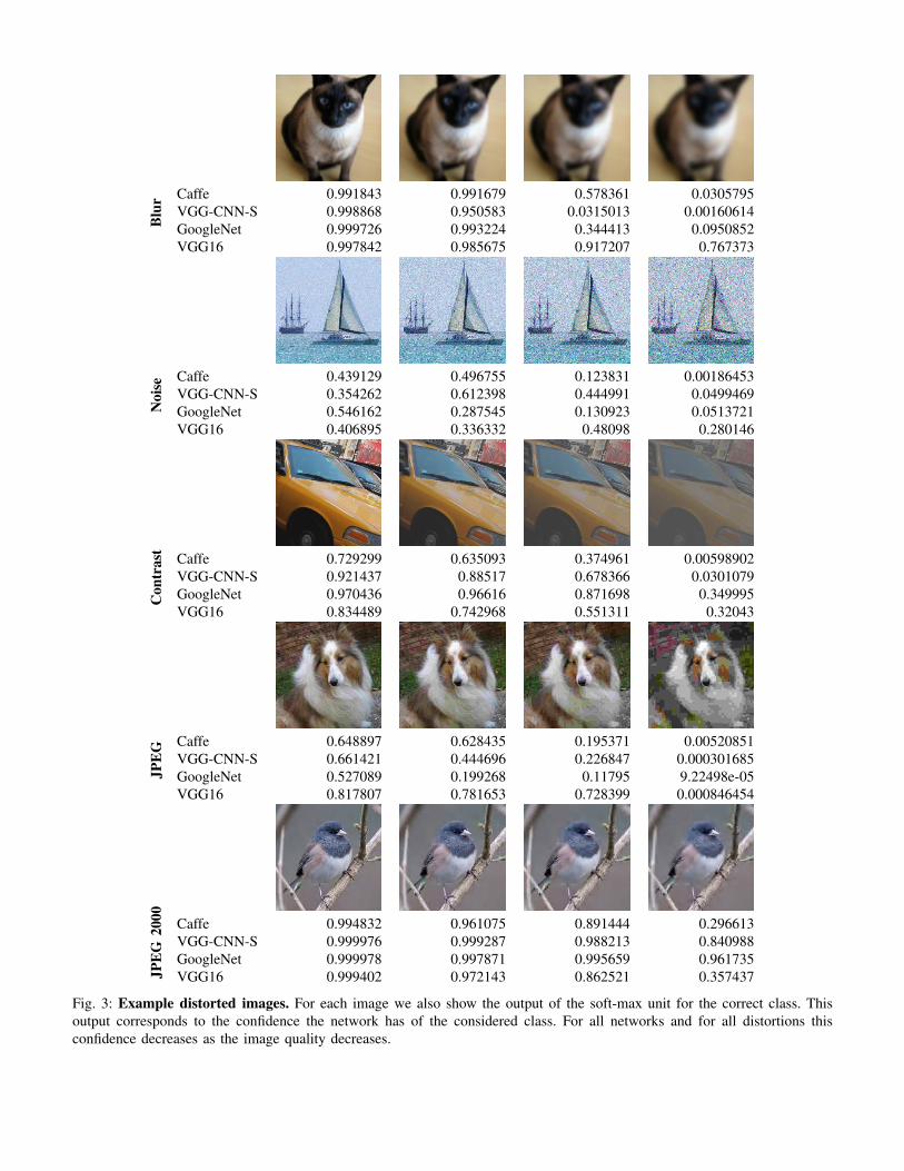
Blu

r Caffe 0.991843 0.991679 0.578361 0.0305795VGG-CNN-S 0.998868 0.950583 0.0315013 0.00160614GoogleNet 0.999726 0.993224 0.344413 0.0950852VGG16 0.997842 0.985675 0.917207 0.767373

Noi

se Caffe 0.439129 0.496755 0.123831 0.00186453VGG-CNN-S 0.354262 0.612398 0.444991 0.0499469GoogleNet 0.546162 0.287545 0.130923 0.0513721VGG16 0.406895 0.336332 0.48098 0.280146

Con

tras

t Caffe 0.729299 0.635093 0.374961 0.00598902VGG-CNN-S 0.921437 0.88517 0.678366 0.0301079GoogleNet 0.970436 0.96616 0.871698 0.349995VGG16 0.834489 0.742968 0.551311 0.32043

JPE

G Caffe 0.648897 0.628435 0.195371 0.00520851VGG-CNN-S 0.661421 0.444696 0.226847 0.000301685GoogleNet 0.527089 0.199268 0.11795 9.22498e-05VGG16 0.817807 0.781653 0.728399 0.000846454

JPE

G20

00 Caffe 0.994832 0.961075 0.891444 0.296613VGG-CNN-S 0.999976 0.999287 0.988213 0.840988GoogleNet 0.999978 0.997871 0.995659 0.961735VGG16 0.999402 0.972143 0.862521 0.357437

Fig. 3: Example distorted images. For each image we also show the output of the soft-max unit for the correct class. Thisoutput corresponds to the confidence the network has of the considered class. For all networks and for all distortions thisconfidence decreases as the image quality decreases.

Conv1-1

Conv5-3

(a) Original (b) Blur (c) Noise

Original Image

Fig. 4: Filter outputs from the VGG16 network on the first (conv1-1) and last (conv5-3) convolutional layers. Blur does notsignificantly affect the early filter responses, yet the filter responses at the last layer can be quite different as compared to thelast layer of the original undistorted image. Noise gives rise to many activations in the first layer, which also propagate to theresponses in the last layer.

low quality images should improve testing results on lowquality images, but perhaps this may also result in decreasedperformance on high quality images. Furthermore, trainingwith increased number of samples leads to longer trainingtimes. An investigation of the benefits of training with lowquality samples is left for future work.

Our results also show that the VGG-16 network[5] exhibitsthe best performance in terms of classification accuracy andresilience for all types and levels of distortions as comparedto the other networks.

ACKNOWLEDGMENT

The authors would like to thank NVIDIA Corporation forthe donation of a TITAN X GPU.

REFERENCES

[1] I. J. Goodfellow, J. Shlens, and C. Szegedy, “Explaining and harnessingadversarial examples,” International Conference on Learning Represen-tations (ICLR), 2015.

[2] J. Wright, A. Y. Yang, A. Ganesh, S. S. Sastry, and Y. Ma, “Robust facerecognition via sparse representation,” Pattern Analysis and MachineIntelligence, IEEE Transactions on, vol. 31, no. 2, pp. 210–227, 2009.

[3] A. S. Razavian, H. Azizpour, J. Sullivan, and S. Carlsson, “Cnn featuresoff-the-shelf: An astounding baseline for recognition,” CVPR Workshopon Deep learning in Computer Vision, pp. 806–813, 2014.

[4] A. Krizhevsky, I. Sutskever, and G. E. Hinton, “Imagenet classificationwith deep convolutional neural networks,” in Advances in neural infor-mation processing systems, 2012, pp. 1097–1105.

[5] K. Simonyan and A. Zisserman, “Very deep convolutional networks forlarge-scale image recognition,” International Conference on LearningRepresentations, 2014.

[6] C. Szegedy, W. Zaremba, I. Sutskever, J. Bruna, D. Erhan, I. Goodfellow,and R. Fergus, “Intriguing properties of neural networks,” InternationalConference on Learning Representations, 2014.

[7] W. W. Zou and P. C. Yuen, “Very low resolution face recognitionproblem,” Image Processing, IEEE Transactions on, vol. 21, no. 1, pp.327–340, 2012.

[8] C.-X. Ren, D.-Q. Dai, and H. Yan, “Coupled kernel embedding forlow-resolution face image recognition,” Image Processing, IEEE Trans-actions on, vol. 21, no. 8, pp. 3770–3783, 2012.

[9] L. J. Karam and T. Zhu, “Quality labeled faces in the wild (qlfw): adatabase for studying face recognition in real-world environments,” inIS&T/SPIE Electronic Imaging. International Society for Optics andPhotonics, 2015, pp. 93 940B1–93 940B10.

[10] J. Tao, W. Hu, and S. Wen, “Multi-source adaptation joint kernel sparserepresentation for visual classification,” Neural Networks, vol. 76, pp.135–151, 2016.

[11] S. Basu, M. Karki, S. Ganguly, R. DiBiano, S. Mukhopadhyay, andR. Nemani, “Learning sparse feature representations using probabilisticquadtrees and deep belief nets,” European Symposium on ArtificialNeural Networks, ESANN, pp. 367–375, 2015.

[12] S. Ullman, L. Assif, E. Fetaya, and D. Harari, “Atoms of recognition inhuman and computer vision,” Proceedings of the National Academy ofSciences, pp. 2744–2749, 2016.

[13] O. Russakovsky, J. Deng, H. Su, J. Krause, S. Satheesh, S. Ma,Z. Huang, A. Karpathy, A. Khosla, M. Bernstein, A. C. Berg, andL. Fei-Fei, “ImageNet Large Scale Visual Recognition Challenge,”International Journal of Computer Vision (IJCV), vol. 115, no. 3, pp.211–252, 2015.

[14] I. Goodfellow, Y. Bengio, and A. Courville, Deep Learning, 2016, mITPress. [Online]. Available: http://goodfeli.github.io/dlbook/

[15] V. Nair and G. E. Hinton, “Rectified linear units improve restricted boltz-mann machines,” in Proceedings of the 27th International Conferenceon Machine Learning (ICML-10), 2010, pp. 807–814.

[16] D. Rumelhard, G. Hinton, and R. Williams, “Learning representationsby back-propagating errors,” Nature, vol. 323, pp. 533–536, 1986.

[17] Y. Jia, E. Shelhamer, J. Donahue, S. Karayev, J. Long, R. Girshick,S. Guadarrama, and T. Darrell, “Caffe: Convolutional architecture forfast feature embedding,” arXiv preprint arXiv:1408.5093, 2014.

[18] K. Chatfield, K. Simonyan, A. Vedaldi, and A. Zisserman, “Return ofthe devil in the details: Delving deep into convolutional nets,” BritishMachine Vision Conference, 2014.

[19] C. Szegedy, W. Liu, Y. Jia, P. Sermanet, S. Reed, D. Anguelov, D. Erhan,V. Vanhoucke, and A. Rabinovich, “Going deeper with convolutions,”CVPR, pp. 1–9, 2015.

[20] P. Haeberli and D. Voorhies, “Image processing by linear interpolationand extrapolation,” IRIS Universe Magazine, vol. 28, pp. 8–9, 1994.