NBER WORKING PAPER SERIES

UNDERSTANDING INFLATION IN INDIA

Laurence BallAnusha ChariPrachi Mishra

Working Paper 22948http://www.nber.org/papers/w22948

NATIONAL BUREAU OF ECONOMIC RESEARCH1050 Massachusetts Avenue

Cambridge, MA 02138December 2016

Prepared for the Brookings-NCAER India Policy Forum. We would like to thank Pami Dua, Subir Gokarn, Ken Kletzer, and participants at the India Policy Forum conference for comments, and Edmund Crawley, Manzoor Gill, Jianhui Li, Wasin Siwasarit, and Ray Wang for excellent research assistance. The views represent those of the authors and not of the Reserve Bank of India, any of the institutions to which the authors belong, or the National Bureau of Economic Research.

NBER working papers are circulated for discussion and comment purposes. They have not been peer-reviewed or been subject to the review by the NBER Board of Directors that accompanies official NBER publications.

© 2016 by Laurence Ball, Anusha Chari, and Prachi Mishra. All rights reserved. Short sections of text, not to exceed two paragraphs, may be quoted without explicit permission provided that full credit, including © notice, is given to the source.

Understanding Inflation in IndiaLaurence Ball, Anusha Chari, and Prachi MishraNBER Working Paper No. 22948December 2016JEL No. E31,E58,F0

ABSTRACT

This paper examines the behavior of quarterly inflation in India since 1994, both headline inflation and core inflation as measured by the weighted median of price changes across industries. We explain core inflation with a Phillips curve in which the inflation rate depends on a slow-moving average of past inflation and on the deviation of output from trend. Headline inflation is more volatile than core: it fluctuates due to large changes in the relative prices of certain industries, which are largely but not exclusively industries that produce food and energy. There is some evidence that changes in headline inflation feed into expected inflation and future core inflation. Several aspects of India’s inflation process are similar to inflation in advanced economies in the 1970s and 80s.

Laurence BallDepartment of EconomicsJohns Hopkins UniversityBaltimore, MD 21218and NBERlball@jhu.edu

Anusha Chari301 Gardner HallCB#3305, Department of EconomicsUniversity of North Carolina at Chapel HillChapel Hill, NC 27599and NBERachari@unc.edu

Prachi MishraReserve Bank of IndiaCentral Office Building,Shahid Bhagat Singh Road, Fort,Mumbai, Maharashtra 400001, Indiaprachimishra@rbi.org.in

2

I. INTRODUCTION

“Inflation poses a serious threat to the growth momentum. Whatever be the cause, the fact remains that inflation is

something which needs to be tackled with great urgency …”

[Dr. Manmohan Singh, Prime Minister of India, February 4, 2011, New Delhi]

Over the last decade, inflation has emerged as a leading concern of India’s economic policymakers

and citizens. Worries grew as the inflation rate (measured as the twelve-month change in the

consumer price index) rose from 3.7% to 12.1% over 2001-2010. The inflation rate has since fallen

to 5.2% in early 2015, leading to a debate about whether this moderation is likely to endure or

inflation will rise again.

What explains the movements in India’s inflation rate? Economists, policymakers, and journalists

have proposed a variety of answers to this question. Many emphasize the effects of rises and falls in

food price inflation, especially for certain staples such as pulses, milk, fruits, and vegetables.2 These

price increases are in turn explained by factors including shifting dietary patterns, rising rural wages,

and a myriad of government policies such as price supports and the rural unemployment guarantee

scheme (Rajan, 2014). Some suggest that the monetary and fiscal stimulus following the crisis led to

higher inflation, while others cite supply side constraints arising from policy bottlenecks (Economic

Survey, 2013).

Many, including RBI Governor Rajan, fear that high levels of inflation may become embedded in

the expectations of price setters, creating a self-sustaining “inflationary spiral” (Rajan, 2014). The

role of monetary policy is controversial, with media reports and analysts debating the role of

interest-rate increases in explaining the recent fall in inflation, and more generally the RBI’s ability to

control inflation and the effects on the real economy (Bhalla, 2014, and Lahiri, 2014).

2 Gokarn (2011), for example, analyzes the micro-level price dynamics of the major dietary sources of protein in India.

3

The debates about inflation in India are reminiscent of debates that have been going on for decades

in advanced economies--especially debates about the 1970s and 1980s, when inflation in the U.S.

and Europe reached double-digit rates, like India more recently. These debates have spurred a large

body of research on inflation, especially in the United States. We draw on this literature to explore

inflation in India. One broad theme is that, despite the differences between the Indian and U.S.

economies, the factors driving inflation fluctuations are similar in many respects.

Section II of this paper explores a central issue in discussions of inflation: the distinction between

headline and core inflation. Core inflation captures the underlying trend in inflation, and headline

inflation fluctuates around core because of large changes in the relative prices of certain goods—

price changes that are often called “supply shocks.” We follow an approach to measuring core

inflation developed by the Federal Reserve Bank of Cleveland: core inflation is measured by the

weighted median of price changes across industries. To implement this approach for India, we

examine the inflation rate in the wholesale price index (WPI). WPI inflation is highly disaggregated

by sector, allowing us to compute a historical series for median inflation.

We find that weighted median inflation is substantially less volatile at the quarterly frequency than

headline inflation, a result that researchers have found for many other countries. We also have a

finding that is not typical of other countries: the average level of median inflation (about 3.4 percent

per year since 1994) is substantially lower than the average level of headline inflation (5.6 percent).

This difference arises because the distribution of price changes across industries is often skewed to

the right—there is a tail of large price increases that raise headline inflation, but are filtered out of

the median—and the distribution is rarely skewed to the left. Many of the large price increases that

raise headline WPI inflation--but far from all of them--occur for different types of food and fuel.

The role of food prices is consistent with the common view that these prices strongly influence

aggregate inflation.

Section III explores the determinants of core inflation. We estimate a version of a standard inflation

equation in textbooks, and in a large body of empirical research: a Phillips curve. In this equation,

core inflation at the quarterly frequency depends on expected inflation, which is determined by past

levels of inflation; and by the level of economic activity, as captured by the deviation of output from

4

its long run trend. Our estimates of the Phillips curve are somewhat imprecise compared to

estimates for advanced economies, reflecting the facts that the necessary data are available only since

1996, and that they are noisy, with substantial quarter-to-quarter movements in weighted median

inflation. Nonetheless, the data point to two conclusions about India’s Phillips curve:

First, current core inflation depends on many lags of past inflation with weights that decline slowly.

We interpret this finding as reflecting slow adjustment of expected inflation. In particular, we

estimate that a one-percentage-point deviation of inflation from its expected level changes expected

inflation in the next quarter by only 0.1 percentage points. This inertia in expectations is consistent

with the view that, once a high level of inflation becomes embedded in expectations, it is not easy to

reduce.

Second, for a given level of expected inflation, there is a positive relationship between inflation and

the deviation of output from trend. This effect is central to the textbook Phillips curve, but some

previous work has questioned it for India.3 Along with our finding about the slow adjustment of

expectations, the estimated effect of output implies that monetary policy can reduce inflation, but

with a short-run cost in output. In particular, we estimate a sacrifice ratio—the loss in percentage

points of annual output needed for a permanent one-point fall in inflation--of approximately 2.7.

This estimate is the same order of magnitude as sacrifice ratios for other economies.

Section IV studies the dynamic interactions among core inflation, headline inflation, and supply

shocks. One finding is that movements in headline inflation appear to influence expected inflation

and hence future levels of core inflation. As a result, a one-time supply shock, such as a large spike

in food prices, can have a persistent effect on inflation. Like other aspects of India’s inflation, this

finding is reminiscent of inflation in advanced economies in the 1970s and 80s.

Section V concludes. We have used data on weighted median inflation to find a Phillips curve for

3 There is a significant body of literature going back at least to Rangarajan (1983) and Dholakia (1990) that estimates Phillips curve for India. Most of the early literature uses annual data, and does not find much evidence for the existence of a short-run trade-off between inflation and output. See also Chaterji (1989), Rangarajan and Arif (1990), Das (2003), Virmani (2004), Bhattacharya and Lodh (1990), Balakrishnan (1991), Callen and Chang (1999), Nachane and Laxmi (2002), Brahmananda and Nagaraju (2002), and Srinivasan et. al. (2006). However, more recently several studies have used quarterly data and demonstrated the existence of a positive relationship between output gap and inflation. Dua and Gaur (2009), Mazumder (2011), Patra and Kapur (2012), Kapur (2013), Kotia (2013), and Das (2014) are recent studies on the topic.

5

India and estimate its slope, which we cannot do with headline inflation because of its quarterly

volatility. Understanding the Phillips curve is essential for effective policies to control inflation.

II. CORE INFLATION AND SUPPLY SHOCKS

Here we discuss the decomposition of headline inflation into core inflation and supply shocks,

which is common in studies of inflation, and apply these concepts to quarterly data for India since

1994.

A. Background

By “core inflation,” economists and central bankers mean an underlying trend in the inflation rate

determined by inflation expectations and the level of economic activity, a trend that follows a

relatively smooth path. The headline inflation rate is the sum of core inflation and “supply shocks,”

which reflect large changes in the prices of particular industries. Headline inflation is more volatile

than core inflation.

The most common measure of supply shocks in empirical work is the change in the relative price of

food and energy. Consistent with this practice, core inflation is often measured by the inflation rate

excluding the prices of food and energy. This practice is motivated by the fact that food and energy

prices are volatile, and excluding them produces a much smoother inflation series.

However, from a theoretical point of view, it is arbitrary to choose certain industries as the source of

supply shocks, and to exclude from measures of core inflation. Ball and Mankiw (1995) define

supply shocks as unusually large changes in the prices of any industries. They suggest that supply

shocks be measured by the degree of asymmetry in the distribution of price changes across

industries. If there is a tail of unusually large price increases, skewing the distribution to the right,

that is a supply shock that raises inflation; a tail of unusually large price decreases has the opposite

effect. Ball and Mankiw motivate this view of supply shocks with models of costly price adjustment,

in which large changes in firms’ desired relative prices have disproportionately large effects on

6

inflation, because they trigger price adjustment while other prices are sticky. 4

If supply shocks reflect asymmetries in the distribution of price changes, then a measure of core

inflation should strip away the effects of these asymmetries—it should eliminate the effects of the

tails of the price distribution. A simple measure that does that is the weighted median of price

changes across industries. This measure of core inflation is proposed by Bryan and Cecchetti (1994),

and the Federal Reserve Bank of Cleveland maintains a measure of weighted median inflation for

the United States.

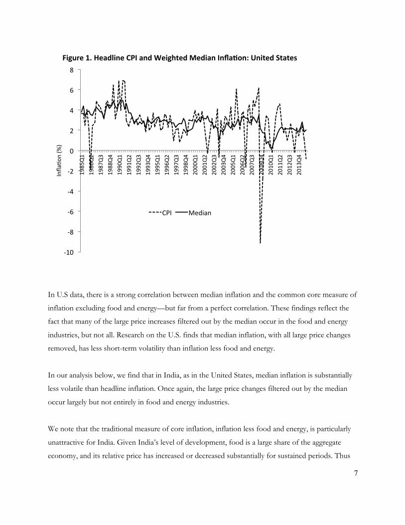
Figure 1 (based on Ball and Mazumder, 2014) illustrates these ideas for the United States by

comparing headline CPI inflation to the weighted median of price changes across U.S. industries, for

the period 1985-2014. We see that the weighted median filters out much of the quarter-to-quarter

volatility in headline inflation, suggesting that it is a good measure of core inflation.

4 Although unusually large changes in the prices are assumed to be caused by “supply shocks” in Ball and Mankiw (1995), a tail of unusually large price increases, in our framework, has the same effect on the price-change distribution, and hence on inflation, regardless of whether it is determined by demand or supply factors. Gokarn (1997), for example, also examines the behavior of the skewness of the distribution of relative price changes in India over the period from 1982-1996, and interprets the skewness to be caused by supply shocks. See more on this later.

7

In U.S data, there is a strong correlation between median inflation and the common core measure of

inflation excluding food and energy—but far from a perfect correlation. These findings reflect the

fact that many of the large price increases filtered out by the median occur in the food and energy

industries, but not all. Research on the U.S. finds that median inflation, with all large price changes

removed, has less short-term volatility than inflation less food and energy.

In our analysis below, we find that in India, as in the United States, median inflation is substantially

less volatile than headline inflation. Once again, the large price changes filtered out by the median

occur largely but not entirely in food and energy industries.

We note that the traditional measure of core inflation, inflation less food and energy, is particularly

unattractive for India. Given India’s level of development, food is a large share of the aggregate

economy, and its relative price has increased or decreased substantially for sustained periods. Thus

!10$

!8$

!6$

!4$

!2$

0$

2$

4$

6$

8$1985Q1$

1986Q2$

1987Q3$

1988Q4$

1990Q1$

1991Q2$

1992Q3$

1993Q4$

1995Q1$

1996Q2$

1997Q3$

1998Q4$

2000Q1$

2001Q2$

2002Q3$

2003Q4$

2005Q1$

2006Q2$

2007Q3$

2008Q4$

2010Q1$

2011Q2$

2012Q3$

2013Q4$

Infla2o

n$(%

)$Figure'1.'Headline'CPI'and'Weighted'Median'Infla7on:'United'States''

CPI$ Median$

8

stripping out food prices leaves an inflation series that wanders far away from the headline inflation

rate that is the ultimate concern of policymakers; it does not just dampen quarterly fluctuations in

inflation.

B. Application to India

Here we begin to describe our empirical analysis for India. For some aspects of our approach, we

outline what we do and provide details in the Appendix to the paper. The measures of inflation that

we study are the rate of change in the headline wholesale price index (WPI), and core inflation in the

WPI as measured by the weighted median inflation rate. We study the WPI because, starting in 1994,

it has a relatively high level of disaggregation into industry inflation rates, which is critical for

measuring median inflation. We note that the Central Statistical Organization began releasing

disaggregated CPI data in 2014. In the future, these data could be used to compare headline and

median inflation based on the CPI.

Historically, the Wholesale Price Index (WPI) has been the most commonly used price index for

measuring inflation in India.5 Our raw data are monthly WPI prices disaggregated by industry from

April 1994 through December 2014. We aggregate across three month periods to create quarterly

series from 1994Q2 through 2014Q4.

For each quarter, the headline inflation rate for the WPI is approximately the mean of inflation rates

across industries, weighted by the importance of the industries.6 We compare this inflation rate, as

reported in official statistics, to the weighted median of inflation rates across industries—the

inflation rate such that industries with 50% of the total weights have higher inflation rates, and the

others have lower rates. The set of industries and weights in the WPI are revised every decade, so

our sample comprises a subsample from 1994Q3 through 2004Q1 with 61 industries and one from

5 The term “wholesale” in the index is however misleading in that the index does not necessarily measure prices in the wholesale market. In practice, the WPI in India measures prices at different stages of the value chain. As discussed in Srinivasan (2008), according to the National Statistical Commission (NSC, 2001), “in many cases, these prices correspond to farm-gate, factory-gate or mine-head prices; and in many other cases, they refer to prices at the level of primary markets, secondary markets or other wholesale or retail markets”. 6 We computed the weighted mean of price changes across industries. As one would expect, this series closely follows the inflation rate calculated from the official series for the WPI.

9

2004Q2 through 2014Q4 with 81 industries. Given the discontinuity in the series, an approximation

is needed to compute the inflation rate in 2004Q2, the first quarter with the revised set of industries

(see Appendix for details). We use the second level of disaggregation that is available. Examples of

industries include primary articles such as Food (Grains:Cereals) and Minerals (Metallic) as well as

manufacturing such as textiles (Cotton: Yarn) and electrical apparatus and appliances.

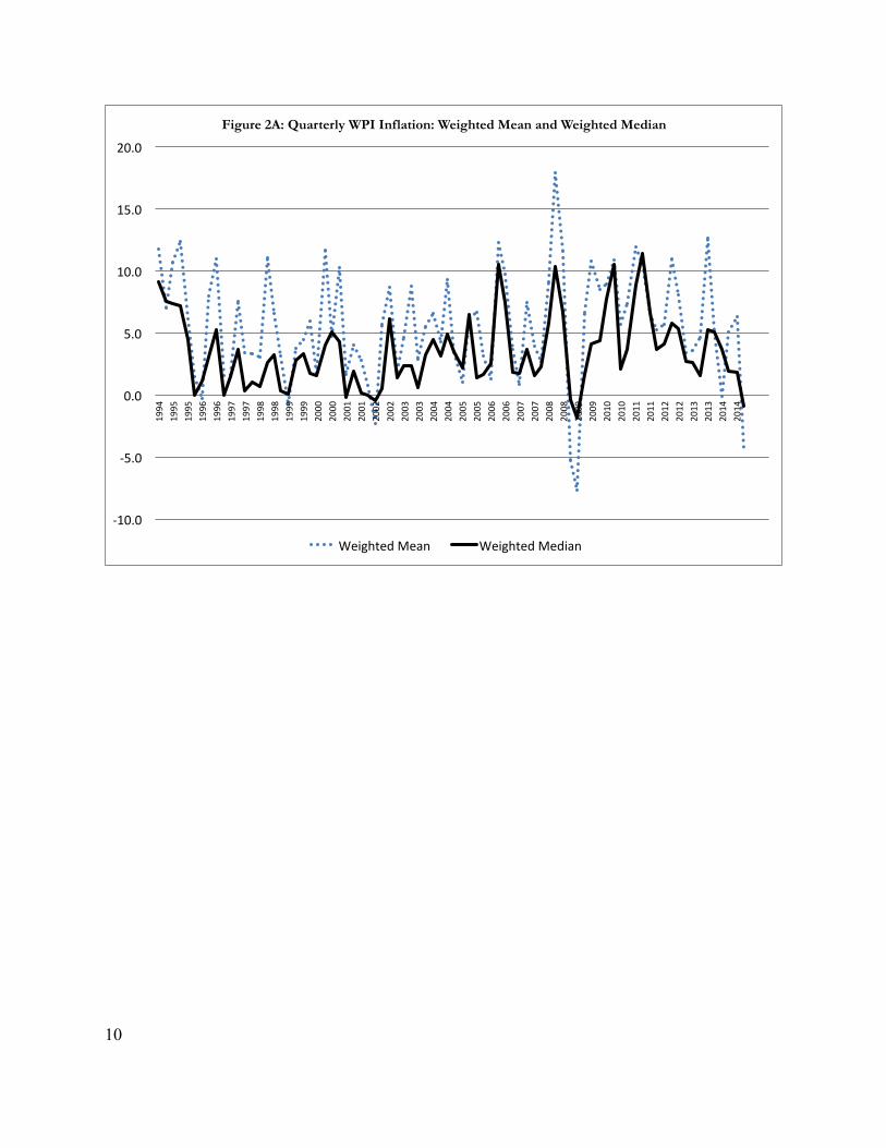
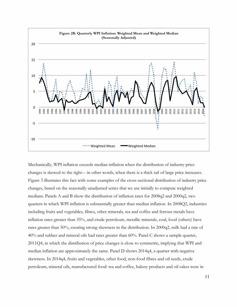
Figure 2 shows the series for official WPI inflation and weighted median inflation, with all quarterly

inflation rates annualized by multiplying by 4. Panel A shows the series we construct from our raw

data, which is not seasonally adjusted, and Panel B shows series that are seasonally adjusted with the

X-13 Arima-Seats procedure from the U.S. Census Bureau. The seasonally adjusted and unadjusted

series are highly correlated (correlation = 0.9 for median inflation), but the seasonally adjusted series

are somewhat less volatile.

As expected, weighted median inflation is substantially less volatile than headline WPI inflation. For

our seasonally adjusted series, the standard deviation of WPI inflation is 3.93% while the standard

deviation of the weighted median is 2.62% between 1994q2 and 2014q4.

We also find that the average level of median inflation over the sample, 3.43 percent, is substantially

lower than the average level of WPI inflation, 5.56 percent. As we see in the Figure, this result

reflects the fact that WPI inflation often spikes up above median inflation, whereas median inflation

is almost never substantially above WPI inflation (with only a few exceptions e.g. 2008Q4 and

2009Q1). This result is surprising, because in other economies median inflation fluctuates fairly

symmetrically around headline inflation and the average levels are similar, as shown for the U.S. in

Figure 1.

10

!10.0%

!5.0%

0.0%

5.0%

10.0%

15.0%

20.0%1994%

1995%

1995%

1996%

1996%

1997%

1997%

1998%

1998%

1999%

1999%

2000%

2000%

2001%

2001%

2002%

2002%

2003%

2003%

2004%

2004%

2005%

2005%

2006%

2006%

2007%

2007%

2008%

2008%

2009%

2009%

2010%

2010%

2011%

2011%

2012%

2012%

2013%

2013%

2014%

2014%

Figure 2A: Quarterly WPI Inflation: Weighted Mean and Weighted Median

Weighted%Mean% Weighted%Median%

11

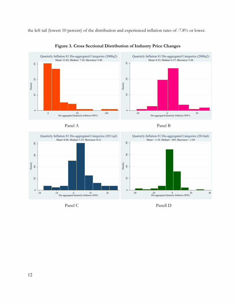
Mechanically, WPI inflation exceeds median inflation when the distribution of industry price

changes is skewed to the right–- in other words, when there is a thick tail of large price increases.

Figure 3 illustrates this fact with some examples of the cross-sectional distribution of industry price

changes, based on the seasonally unadjusted series that we use initially to compute weighted

medians. Panels A and B show the distribution of inflation rates for 2008q2 and 2000q2, two

quarters in which WPI inflation is substantially greater than median inflation. In 2008Q2, industries

including fruits and vegetables, fibres, other minerals, tea and coffee and ferrous metals have

inflation rates greater than 35%, and crude petroleum, metallic minerals, coal, food (others) have

rates greater than 50%, creating strong skewness in the distribution. In 2000q2, milk had a rate of

40% and rubber and mineral oils had rates greater than 60%. Panel C shows a sample quarter,

2011Q4, in which the distribution of price changes is close to symmetric, implying that WPI and

median inflation are approximately the same. Panel D shows 2014q4, a quarter with negative

skewness. In 2014q4, fruits and vegetables, other food, non-food fibres and oil seeds, crude

petroleum, mineral oils, manufactured food: tea and coffee, bakery products and oil cakes were in

!10$

!5$

0$

5$

10$

15$

20$1994$

1995$

1995$

1996$

1996$

1997$

1997$

1998$

1998$

1999$

1999$

2000$

2000$

2001$

2001$

2002$

2002$

2003$

2003$

2004$

2004$

2005$

2005$

2006$

2006$

2007$

2007$

2008$

2008$

2009$

2009$

2010$

2010$

2011$

2011$

2012$

2012$

2013$

2013$

2014$

2014$

Figure 2B: Quarterly WPI Inflation: Weighted Mean and Weighted Median (Seasonally Adjusted)

Weighted$Mean$ Weighted$Median$

12

the left tail (lowest 10 percent) of the distribution and experienced inflation rates of -7.8% or lower.

Figure 3. Cross Sectional Distribution of Industry Price Changes

Panel A Panel B

Panel C Panell D

0.0

1.0

2.0

3D

ensi

ty

0 50 100Dis-aggregated Quarterly Inflation (WP1)

Mean=13.82; Median= 7.26; Skewness=3.08Quarterly Inflation 81 Dis-aggregated Categories (2008q2)

0.0

1.0

2.0

3D

ensi

ty

-50 0 50Dis-aggregated Quarterly Inflation (WP1)

Mean=4.33; Median=2.37; Skewness=1.04Quarterly Inflation 81 Dis-aggregated Categories (2000q2)

0.0

2.0

4.0

6.0

8D

ensi

ty

-20 -10 0 10 20Dis-aggregated Quarterly Inflation (WPI)

Mean=4.04; Median=3.25; Skewness=0.21Quarterly Inflation 81 Dis-aggregated Categories (2011q4)

0.0

2.0

4.0

6.0

8D

ensi

ty

-40 -20 0 20 40Dis-aggregated Quartery Inflation (WPI)

Mean= -1.18; Median= .085; Skewness= -1.04Quarterly Inflation 81 Dis-aggregated Categories (2014q4)

13

C. The Role of Food and Fuel Prices

Changes in food and fuel prices cause many of the episodes of skewed price change distributions in

India, as suggested by the example of 2008q2. The same is true in advanced economies. To

demonstrate this point systematically, we examine the industries that account for the top ten percent

of the weighted distribution of inflation rates in each quarter—the right tail of the distribution,

which creates skewness in many quarters and raises WPI inflation above median inflation. Many of

these industries are producers of various kinds of food and fuel, such as fruits, vegetables, milk,

crude petroleum, coal, and electricity. For each of our industries, we examine its contribution to the

right tail of the distribution for each quarter. This contribution is zero if the industry is not in the

10% tail; the industry’s WPI weight times ten if it is in the tail; and somewhere in between if the

industry’s price change puts it at the border of the top 10%, in which case part of the industry’s

weight is included in the tail. For each industry, we compute the average contribution to the 10% tail

over our 82 quarterly observations on prices. These average contributions sum to 100%.

Recall there are 81 industries for the second part of our sample period; of these, 18 are different

types of food (both primary articles and manufactured food) and 4 are different types of fuel or

power. To see the influence of these industries more clearly, we aggregate them by one level into

three broad industries: primary articles: food, manufacturing: food, and fuel and power. We also

aggregate the other industries one level leaving us with 15 industries. For each of these industries,

Table 1 shows the total of the average contributions of it components to the top ten percent of

price changes.

The results are striking. The three food and fuel industries are the three largest contributors to the

ten percent tail, with a contribution that sums to 63.5 percent. Notice if we add in non-food

commodities, the fourth largest contributor, the total rises to 72 percent. Thus if inflationary supply

shocks are captured by right-skewness in the price-change distribution, Indian data confirm the

common view that a large share of supply shocks originate in food and fuel industries—but not all.

Notice that metals, chemicals, and textiles also are significant contributors to the ten percent tail.

14

Figure 4 illustrates the importance of food and fuel in a different way. It shows two series: the

difference between WPI inflation and median inflation, which captures the asymmetry in the

distribution of price changes; and the change in the relative price of food and fuel, calculated as

average inflation for food and fuel minus WPI inflation. We can see that the two series have a strong

positive relationship. For the non-seasonally adjusted series shown here, the correlation is 0.60. The

correlation is somewhat lower, 0.41, when we seasonally adjust both series. Once again, we see that

increases in food and fuel prices explain a large share but not all of the right tails in the distribution

of inflation rates.

Industry Rescaled.Weighted.Frequency!!Primary!Articles:!Food 27.83!!Fuel!&!Power 23.50!!Mfg:!Food 12.22!!Primary!Articles:!Non!Food 8.50!!Mfg:!BM:!Basic!Metals,!Alloys!and!Metal!Products 7.55!!Mfg:!CC:!Chemicals!&!Chemical!Products! 6.02!!Mfg:!Textiles 4.46!!Primary!Articles:!Minerals 2.31!!Mfg:!NM:!Non!Metallic!Mineral!Products 1.95!!Mfg:!Paper!&!Paper!Products 1.21!!Mfg:!MM:Machinery!&!Machine!Tools 0.96!!Mfg:!BT:!Beverages,!Tobacco!&!Tobacco!Products 0.95!!Mfg:!TE:!Transport,!Equipment!&!Parts 0.93!!Mfg:!Rubber!&!Plastic 0.85!!Mfg:!Leather!&!Leather!Products!(LL) 0.52!!Mfg:!Wood!Wood!Products 0.25

Table 1. Contributors to Top 10% of Price Changes

Notes.!Weighted!frequency!is!rescaled!to!sum!to!100.!Industries!are!sorted!By!weighted!frequency.!Total!number!of!quarters=82!(1994q3:2014q4)

15

III. A PHILLIPS CURVE FOR CORE INFLATION

The canonical Phillips curve explains inflation with expected inflation and the level of economic

activity relative to the economy’s potential. In many applications, researchers assume that expected

inflation can be captured by lagged values of actual inflation. Here we examine the fit of a simple

Phillips curve to core inflation in India, as measured by the weighted median.

Milton Friedman’s Phillips Curve

A large body of research is based on the Phillips curve introduced in Milton Friedman’s Presidential

Address to the AEA (1968). This relation can be written as

(1) 𝜋! = 𝜋!! + 𝛼(𝑥! − 𝑥! ∗) +∈!

!8.0%

!6.0%

!4.0%

!2.0%

0.0%

2.0%

4.0%

6.0%

8.0%

10.0%

!15%

!10%

!5%

0%

5%

10%

15%

20%1994%

1995%

1995%

1996%

1996%

1997%

1997%

1998%

1998%

1999%

1999%

2000%

2000%

2001%

2001%

2002%

2002%

2003%

2003%

2004%

2004%

2005%

2005%

2006%

2006%

2007%

2007%

2008%

2008%

2009%

2009%

2010%

2010%

2011%

2011%

2012%

2012%

2013%

2013%

2014%

2014%

Figure 4. (Mean-Median) WPI inflation & Food+Fuel Inflation -WPI Inflation

Food+Fuel%Infla9on%!%Mean%WPI%Infla9on% (Mean!Median)%Quarterly%WPI%Infla9on%!%Right%Scale%

Correla'on)Coefficient=0.60%

16

where 𝜋! is inflation, 𝜋!! is expected inflation, and 𝑥! is a measure of economic activity, typically

either the log level of output or the unemployment rate. The variable 𝑥! ∗ is the long run level of 𝑥,

which is called the natural rate when 𝑥 is unemployment and potential output when 𝑥 is output. The

term 𝑥! − 𝑥! ∗ captures short-run fluctuations in output or unemployment. The error term ∈!

captures unobservable factors that influence inflation.

This Phillips curve is exposited in leading textbooks in macroeconomics. The expected inflation

term captures the idea that expectations of inflation tend to be self-fulfilling: if price and wage

setters expect a certain level of inflation, they raise their nominal prices to keep up, and in aggregate

their price increases create the inflation they expect. The 𝑥! − 𝑥! ∗ term captures the idea that an

increase in activity relative to the economy’s normal level raises firms’ marginal costs, which causes

them to raise prices by more than they otherwise would.

Here we examine the fit of equation (1) to the behavior of core inflation. In Section IV of this

paper, we examine how core inflation and supply shocks interact to determine the behavior of

headline WPI inflation.

To estimate equation (1), we must choose measures of 𝑥!, 𝑥! ∗, and 𝜋!! .

Measuring Economic Activity

We lack quarterly data on aggregate unemployment for India. Quarterly data on output, however,

are available from the Central Statistical Organization (CSO). In our empirical analysis, we use

quarterly GDP (at market prices) since 1996Q2. We combine the 2004-05 base-year GDP series and

the 1999-2000 series to create a common series from 1996Q2 to 2014Q3, using a commonly used

splicing methodology. The details of the splicing methodology are provided in Appendix 1. We

measure activity 𝑥! with the logarithm of output. Before taking the logarithm, we seasonally adjust

the output series using the U.S. Census Bureau’s X-13 procedure. This adjustment is important

because there are large seasonal movements in India’s output.

17

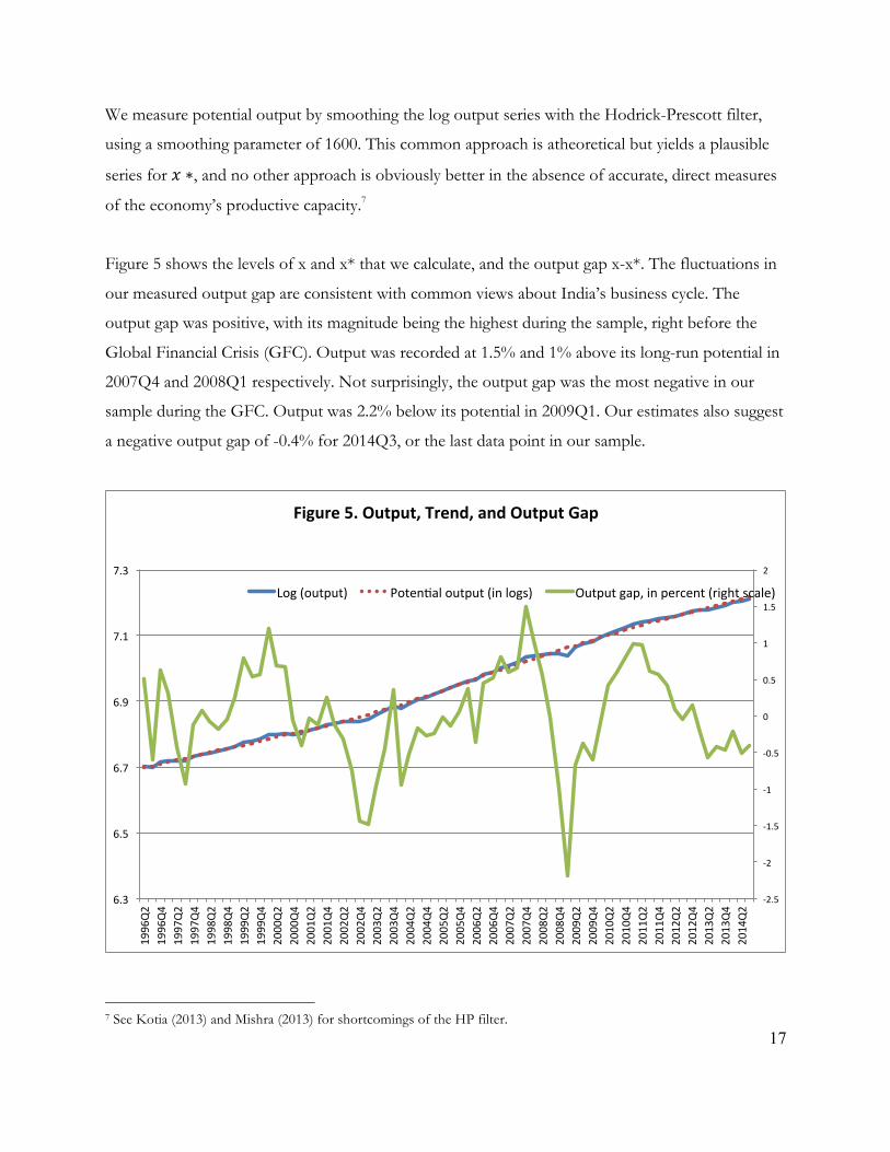
We measure potential output by smoothing the log output series with the Hodrick-Prescott filter,

using a smoothing parameter of 1600. This common approach is atheoretical but yields a plausible

series for 𝑥 ∗, and no other approach is obviously better in the absence of accurate, direct measures

of the economy’s productive capacity.7

Figure 5 shows the levels of x and x* that we calculate, and the output gap x-x*. The fluctuations in

our measured output gap are consistent with common views about India’s business cycle. The

output gap was positive, with its magnitude being the highest during the sample, right before the

Global Financial Crisis (GFC). Output was recorded at 1.5% and 1% above its long-run potential in

2007Q4 and 2008Q1 respectively. Not surprisingly, the output gap was the most negative in our

sample during the GFC. Output was 2.2% below its potential in 2009Q1. Our estimates also suggest

a negative output gap of -0.4% for 2014Q3, or the last data point in our sample.

7 See Kotia (2013) and Mishra (2013) for shortcomings of the HP filter.

!2.5%

!2%

!1.5%

!1%

!0.5%

0%

0.5%

1%

1.5%

2%

6.3%

6.5%

6.7%

6.9%

7.1%

7.3%

1996Q2%

1996Q4%

1997Q2%

1997Q4%

1998Q2%

1998Q4%

1999Q2%

1999Q4%

2000Q2%

2000Q4%

2001Q2%

2001Q4%

2002Q2%

2002Q4%

2003Q2%

2003Q4%

2004Q2%

2004Q4%

2005Q2%

2005Q4%

2006Q2%

2006Q4%

2007Q2%

2007Q4%

2008Q2%

2008Q4%

2009Q2%

2009Q4%

2010Q2%

2010Q4%

2011Q2%

2011Q4%

2012Q2%

2012Q4%

2013Q2%

2013Q4%

2014Q2%

Figure'5.'Output,'Trend,'and'Output'Gap''

Log%(output)% Poten:al%output%(in%logs)% Output%gap,%in%percent%(right%scale)%

18

One questionable feature of the output gap series is that the size of fluctuations is small. The

estimated output gap is never more than one or two percent in absolute value; even in the wake of

the global financial crisis (GFC), the gap reaches only -2%. By contrast, U.S. output gaps as

measured by the HP filter reach levels around 5% in absolute value in deep recessions and strong

expansions. We are not confident that cyclical fluctuations in India are as small as our estimated gaps

suggest, and suspect that the quarterly data reported for real GDP could be smoother than true

GDP. We will keep this issue in mind in interpreting our estimated effects of the output gap on

inflation.8

Measuring Expected Inflation

In presenting his Phillips curve, Friedman said that “unanticipated inflation generally means a rising

rate of inflation.” This is the same as saying that expected inflation is determined by past inflation.

Following Friedman, much of the U.S. Phillips curve literature (e.g. Gordon (1982), Stock and

Watson (2007), Ball and Mazumder (2011)) has used lags of inflation to capture expected inflation.

With quarterly data, researchers typically include a number of inflation lags in the Phillips curve, with

the restriction that the coefficients on the lags sum to one.

In recent years, inflation expectations have appeared to be “anchored” in advanced economies

including the U.S. and Europe. Since around 2000, the Fed and ECB have been targeting inflation

rates near two percent, and expected inflation has stayed close to that level: expectations have not

varied based on lagged values of actual inflation. We doubt, however, that inflation expectations

were anchored in India over our sample period. The RBI formally announced an inflation target

only in 2015. 9 Over our sample, the inflation rate was volatile without a clear tendency to return to

some fixed level, much as inflation rates wandered in the U.S. and Europe between 1960 and 2000.

In such a regime, it is natural to assume that expected inflation responds to lagged values of actual

inflation.

8 Some suggest using a lower HP smoothing parameter for emerging economies. This would produce even smaller estimated output gaps. 9 See http://finmin.nic.in/reports/MPFAgreement28022015.pdf on agreement between Government of India and Reserve Bank of India on new monetary policy framework.

19

As we saw in Figure 2, quarterly core inflation is quite volatile in India–-more volatile than core

inflation in advanced economies. We conjecture that expected inflation is less volatile: a few quarters

of high or low inflation do not change expectations dramatically. To capture this idea, we want to

allow expected inflation to depend on lagged inflation over many quarters. At the same time we do

not want to include numerous lags with unrestricted coefficients; we want a parsimonious Phillips

curve with a minimum of free parameters. These goals lead us to a simple partial-adjustment model

of expectations.

Specifically, we assume that expected inflation is determined by:

(2) 𝜋!! = 𝛾𝜋!!!! + (1− 𝛾)𝜋!!!

In this specification, expected inflation depends on its own lag and the lag of actual inflation with

weights 𝛾 and 1− 𝛾. This implies that a one-percentage point deviation of lagged inflation from its

expected level changes current expected inflation by 1− 𝛾 percentage points. Repeated substitution

for lagged inflation leads to the following reduced form:

(3) 𝜋!! = 1− 𝛾 𝜋!!! + 𝛾 1− 𝛾 𝜋!!! + 𝛾! 1− 𝛾 𝜋!!! + 𝛾! 1− 𝛾 𝜋!!! +⋯ ..

Here, expected inflation depends on all lags of past inflation, with exponentially declining weights.

The adjustment parameter 𝛾 determines the relative weights on recent and less recent inflation rates.

We treat 𝛾 as a parameter to be estimated.

If we write our equation for expected inflation compactly and substitute it into Friedman’s Phillips

curve (1), we get

(4) 𝜋! = (1− 𝛾)[ 𝛾!!!!!!! 𝜋!!!]+ 𝛼(𝑥! − 𝑥! ∗) +∈!

To estimate this equation with the available data, we must make two approximations, which we

describe in Appendix 2. First, we truncate the infinite sum in the theoretical Phillips curve: we

include only 40 lags of inflation with exponentially declining weights, while maintaining the

20

restriction that the weights sum to one.10

Second, we must address the problem that, even with the lags truncated at forty, we do not have

data on median inflation that extends far enough back to include forty lags in the early part of our

sample. In our regressions, the sample starts in 1996Q2, the first quarter for which output data are

available, and our median inflation series extends back only seven quarters before that, to 1994Q3.

Since we cannot measure 𝜋!! for our entire sample, we treat 𝜋!! in 1996Q2 as an unobserved

parameter, which we estimate along with the parameters 𝛾 and 𝛼 in the Phillips curve. We estimate

the initial 𝜋!! , 𝛾 and 𝛼 by non-linear least squares: we find the values of these three parameters that

minimize the sum of squared residuals in the equation. Notice that an estimate of the initial 𝜋!! and

an estimate of 𝛾 allow us to calculate 𝜋!! for all observations in our regression using the partial

adjustment equation (3).

Estimates

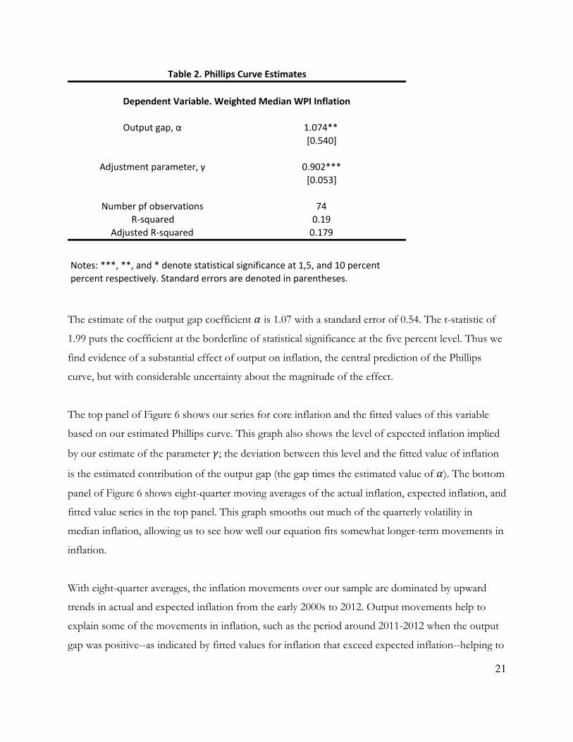
Table 2 presents our estimation results. The estimate of the initial level of expected inflation is about

1.9, and the estimate of 𝛾 is 0.90, with a standard error of 0.05. If we put this estimate into our

reduced-form equation for expected inflation, it implies that the first four inflation lags have

coefficients of approximately 0.1, 0.09, 0.08, and 0.07, which sum to 0.34 out of the total sum of

coefficients of one. This confirms that relatively long lags of inflation—beyond one year—have

substantial weight in determining the current levels of expected and actual inflation, as we

conjectured based on the volatility of quarterly inflation.

10 Some readers of this paper have questioned the structure of inflation lags that we assume, so we have experimented with alternatives. As we expect based on the volatility of inflation, a large number of lags is needed to capture the behavior of expectations. We verify this point by estimating a version of equation (4) in which we replace the exponentially weighted sum of inflation lags with 16 lags with unrestricted coefficients. In this specification, we reject the hypothesis that the coefficients on lags 13-16 are zero (p= 0.0383), which suggests that at least 16 lags are needed to fit the data. At the same time, when we include 16 unrestricted lags, the pattern of estimated coefficients on the lags is erratic, suggesting the model is over-parameterized. These findings confirm the usefulness of restricting the coefficients with our partial adjustment model.

21

The estimate of the output gap coefficient 𝛼 is 1.07 with a standard error of 0.54. The t-statistic of

1.99 puts the coefficient at the borderline of statistical significance at the five percent level. Thus we

find evidence of a substantial effect of output on inflation, the central prediction of the Phillips

curve, but with considerable uncertainty about the magnitude of the effect.

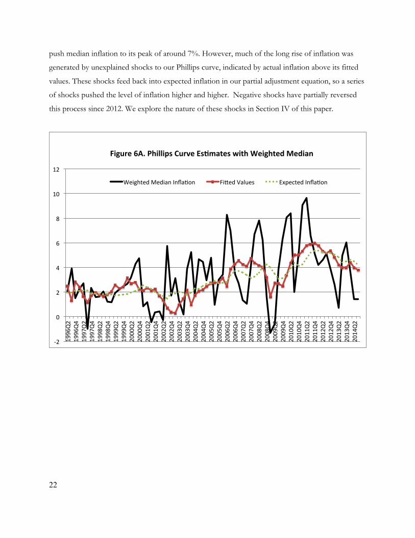
The top panel of Figure 6 shows our series for core inflation and the fitted values of this variable

based on our estimated Phillips curve. This graph also shows the level of expected inflation implied

by our estimate of the parameter 𝛾; the deviation between this level and the fitted value of inflation

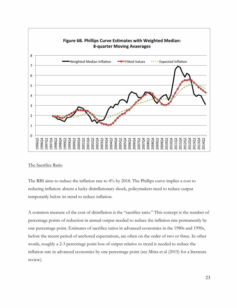
is the estimated contribution of the output gap (the gap times the estimated value of 𝛼). The bottom

panel of Figure 6 shows eight-quarter moving averages of the actual inflation, expected inflation, and

fitted value series in the top panel. This graph smooths out much of the quarterly volatility in

median inflation, allowing us to see how well our equation fits somewhat longer-term movements in

inflation.

With eight-quarter averages, the inflation movements over our sample are dominated by upward

trends in actual and expected inflation from the early 2000s to 2012. Output movements help to

explain some of the movements in inflation, such as the period around 2011-2012 when the output

gap was positive--as indicated by fitted values for inflation that exceed expected inflation--helping to

Output%gap,%α 1.074**[0.540]

Adjustment%parameter,%γ 0.902***[0.053]

Number%pf%observations 74RFsquared 0.19

Adjusted%RFsquared 0.179

Table&2.&Phillips&Curve&Estimates

Dependent&Variable.&Weighted&Median&WPI&Inflation

Notes:%***,%**,%and%*%denote%statistical%significance%at%1,5,%and%10%percent%percent%respectively.%Standard%errors%are%denoted%in%parentheses.

22

push median inflation to its peak of around 7%. However, much of the long rise of inflation was

generated by unexplained shocks to our Phillips curve, indicated by actual inflation above its fitted

values. These shocks feed back into expected inflation in our partial adjustment equation, so a series

of shocks pushed the level of inflation higher and higher. Negative shocks have partially reversed

this process since 2012. We explore the nature of these shocks in Section IV of this paper.

!2#

0#

2#

4#

6#

8#

10#

12#

1996Q2#

1996Q4#

1997Q2#

1997Q4#

1998Q2#

1998Q4#

1999Q2#

1999Q4#

2000Q2#

2000Q4#

2001Q2#

2001Q4#

2002Q2#

2002Q4#

2003Q2#

2003Q4#

2004Q2#

2004Q4#

2005Q2#

2005Q4#

2006Q2#

2006Q4#

2007Q2#

2007Q4#

2008Q2#

2008Q4#

2009Q2#

2009Q4#

2010Q2#

2010Q4#

2011Q2#

2011Q4#

2012Q2#

2012Q4#

2013Q2#

2013Q4#

2014Q2#

Figure'6A.'Phillips'Curve'Es3mates'with'Weighted'Median'''

Weighted#Median#Infla:on# Fi=ed#Values# Expected#Infla:on#

23

The Sacrifice Ratio

The RBI aims to reduce the inflation rate to 4% by 2018. The Phillips curve implies a cost to

reducing inflation: absent a lucky disinflationary shock, policymakers need to reduce output

temporarily below its trend to reduce inflation.

A common measure of the cost of disinflation is the “sacrifice ratio.” This concept is the number of

percentage points of reduction in annual output needed to reduce the inflation rate permanently by

one percentage point. Estimates of sacrifice ratios in advanced economies in the 1980s and 1990s,

before the recent period of anchored expectations, are often on the order of two or three. In other

words, roughly a 2-3 percentage point loss of output relative to trend is needed to reduce the

inflation rate in advanced economies by one percentage point (see Mitra et al (2015) for a literature

review).

0"

1"

2"

3"

4"

5"

6"

7"

8"

1996Q2"

1996Q4"

1997Q2"

1997Q4"

1998Q2"

1998Q4"

1999Q2"

1999Q4"

2000Q2"

2000Q4"

2001Q2"

2001Q4"

2002Q2"

2002Q4"

2003Q2"

2003Q4"

2004Q2"

2004Q4"

2005Q2"

2005Q4"

2006Q2"

2006Q4"

2007Q2"

2007Q4"

2008Q2"

2008Q4"

2009Q2"

2009Q4"

2010Q2"

2010Q4"

2011Q2"

2011Q4"

2012Q2"

2012Q4"

2013Q2"

2013Q4"

2014Q2"

Figure'6B.'Phillips'Curve'Es3mates'with'Weighted'Median:'8>quarter'Moving'Avaerages'

Weighted"Median"Infla9on" Fi<ed"Values" Expected"Infla9on"

24

Using our Phillips curve, we can calculate the sacrifice ratio as follows. A loss of output of one

percentage point for one quarter reduces current inflation by 𝛼 percentage points. Given our

specification of expectations, that fall in inflation reduces expected inflation by (𝛼) ∗ 1− 𝛾 in the

following period. If output returns to normal at that point and there are no shocks to the Phillips

curve, then actual inflation is (𝛼) ∗ 1− 𝛾 below its initial level, and stays there.

Thus a one-point fall in output below normal for one quarter reduces inflation by (𝛼) ∗ 1− 𝛾

points. A one-point fall in output that lasts for four quarters–-a loss of one point of annual output–-

reduces inflation by 4*(𝛼) ∗ 1− 𝛾 . The sacrifice ratio is the inverse of this effect: in order to

reduce the inflation rate by one percentage point, a loss of 1/[4*(𝛼) ∗ 1− 𝛾 ] percentage points of

annual output is required.

Substituting in our estimates of 𝛾 and 𝛼 yields a sacrifice ratio of 2.7, which is the same order of

magnitude as estimates for other countries. If the current level of inflation is 5.2% and the RBI

wishes to reduce it to 4%, the cost will be 1.2*2.7=3.2 percentage points of annual output. Notice

that our estimated sacrifice ratio for India is quite close to estimates by Mitra et al (2015) (around 2.3

or 2.8 depending on the state of the economy), despite large differences between their methodology

and ours.

Two caveats: First, the RBI is targeting CPI inflation, whereas we calculate a sacrifice ratio for core

WPI inflation. Future work should examine whether the relationships of output to CPI and WPI

inflation are similar.

Second, as noted above, we suspect that quarterly output data may understate the size of short-run

fluctuations. If so, the true output gaps associated with given changes in inflation may be larger than

the estimated gaps, which would imply a larger sacrifice ratio.

25

IV. CORE INFLATION, SUPPLY SHOCKS, AND MEDIAN INFLATION

The previous section found that the behavior of India’s core inflation, as measured by weighted

median inflation, can be explained to a significant degree by a simple Phillips curve. We saw earlier,

however, that many of the fluctuations in headline inflation are deviations from core inflation caused

by supply shocks, as measured by asymmetries in the cross-sectional distribution of price changes.

Here we seek a broader understanding of India’s inflation by examining the interactions among core

inflation, headline inflation, and supply shocks. One finding is that movements in headline inflation

appear to influence expected inflation and hence future levels of core inflation. As a result, a one-

time supply shock, such as a large spike in food prices, can have a persistent effect on inflation. Like

other aspects of India’s inflation, this finding is reminiscent of inflation in advanced economies in

the 1970s and 80s.

A Phillips Curve for Headline Inflation?

As a first exercise, we examine how well the simple Phillips curve fits inflation behavior if we ignore

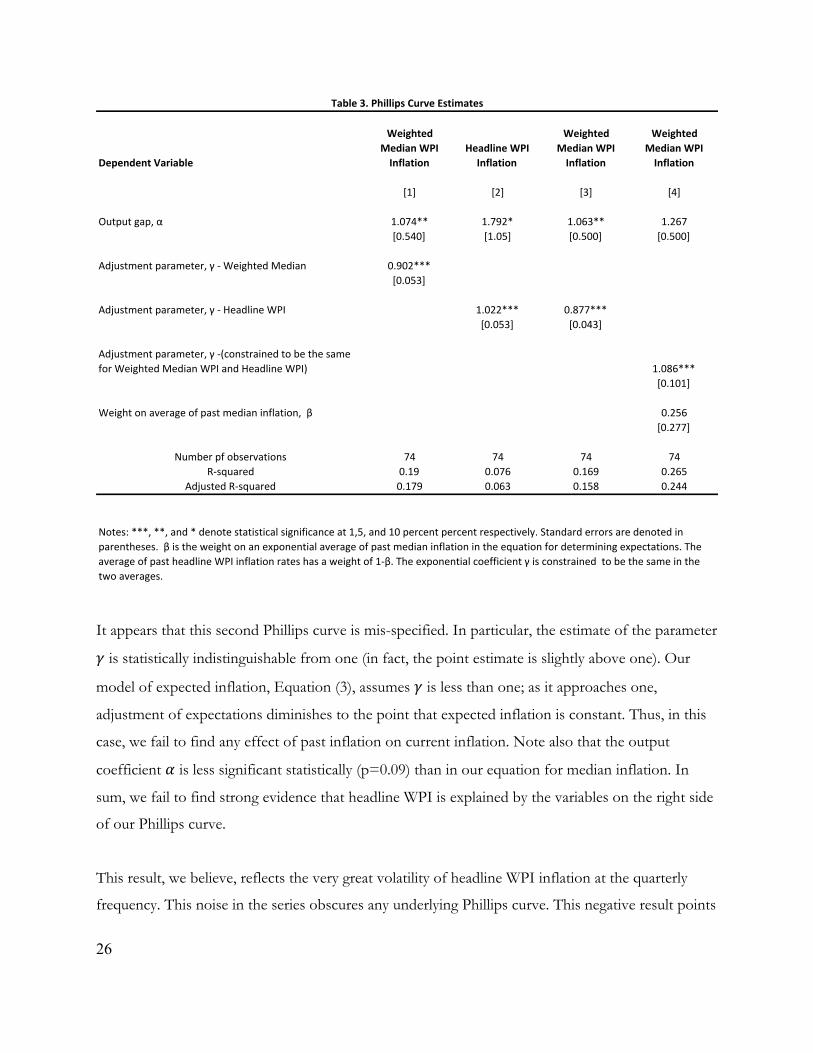
the concept of core inflation and examine the headline WPI. In Table 3, the first column repeats our

Phillips curve for median inflation, for purpose of comparison, and the second column reports

estimates of an equation for headline inflation. This specification is the same as the first except that

the dependent variable is headline WPI inflation and the lagged inflation rates with which we capture

expected inflation are also WPI inflation.

26

It appears that this second Phillips curve is mis-specified. In particular, the estimate of the parameter

𝛾 is statistically indistinguishable from one (in fact, the point estimate is slightly above one). Our

model of expected inflation, Equation (3), assumes 𝛾 is less than one; as it approaches one,

adjustment of expectations diminishes to the point that expected inflation is constant. Thus, in this

case, we fail to find any effect of past inflation on current inflation. Note also that the output

coefficient 𝛼 is less significant statistically (p=0.09) than in our equation for median inflation. In

sum, we fail to find strong evidence that headline WPI is explained by the variables on the right side

of our Phillips curve.

This result, we believe, reflects the very great volatility of headline WPI inflation at the quarterly

frequency. This noise in the series obscures any underlying Phillips curve. This negative result points

Dependent'Variable

Weighted'Median'WPI'Inflation

Headline'WPI'Inflation

Weighted'Median'WPI'Inflation

Weighted'Median'WPI'Inflation

[1] [2] [3] [4]

Output+gap,+α 1.074** 1.792* 1.063** 1.267[0.540] [1.05] [0.500] [0.500]

Adjustment+parameter,+γ+@+Weighted+Median 0.902***[0.053]

Adjustment+parameter,+γ+@+Headline+WPI 1.022*** 0.877***[0.053] [0.043]

Adjustment+parameter,+γ+@(constrained+to+be+the+same+for+Weighted+Median+WPI+and+Headline+WPI) 1.086***

[0.101]

Weight+on+average+of+past+median+inflation,++β 0.256[0.277]

Number+pf+observations 74 74 74 74R@squared 0.19 0.076 0.169 0.265

Adjusted+R@squared 0.179 0.063 0.158 0.244

Table'3.'Phillips'Curve'Estimates

Notes:+***,+**,+and+*+denote+statistical+significance+at+1,5,+and+10+percent+percent+respectively.+Standard+errors+are+denoted+in+parentheses.++β+is+the+weight+on+an+exponential+average+of+past+median+inflation+in+the+equation+for+determining+expectations.+The+average+of+past+headline+WPI+inflation+rates+has+a+weight+of+1@β.+The+exponential+coefficient+γ+is+constrained++to+be+the+same+in+the+two+averages.

27

to the desirability of examining median inflation when estimating the Phillips curve.

Core Inflation, Headline Inflation, and Expectations

Here we return to an equation with median inflation as the dependent variable. However, we

consider the possibility that the lagged inflation terms on the right of the equation are headline WPI

inflation. We interpret such a specification as saying that price setters base their expectations of

inflation on past levels of headline inflation, so that movements in headline inflation are passed into

future core inflation.

It is not clear a priori whether expected inflation should depend on past levels of headline inflation

or past levels of core inflation. Empirically, a number of studies for the United States find a sharp

break in inflation behavior around the Volcker disinflation of the early 1980s. Inflation is explained

by lags of headline inflation before that time, and by lags of core inflation afterwards. The usual

interpretation is that price setters in the 1970s based their expectations on past headline inflation, so

expected inflation responded to movements in headline inflation even if those movements were the

result of transitory supply shocks. After the Volcker disinflation, however, it became clear that the

Federal Reserve was determined to reverse transitory inflation movements due to supply shocks, so

those shocks no longer influenced expectations and actual inflation going forward. In the

terminology of central bankers, in the post-Volcker era, supply shocks have first round effects-they

directly affect current headline inflation-but not second round effects on expectations and future

inflation.

Before using lagged headline inflation rates to explain median inflation, we account for the fact that

headline inflation is systematically higher than median inflation-the difference averages 2.42

percentage points over the sample period for our regressions. We subtract this constant from the

headline WPI series, resulting in an adjusted series with the same average value as the median. We

can interpret this specification as explaining median inflation with lagged levels of headline inflation,

both measured relative to their sample averages.

The third column of Table 3 reports this specification. The results for this case are quite close to

28

those with median inflation on both sides of the equation, in column (1): the estimates of 𝛼 and 𝛾

are similar, and so are the R-squared. The estimate of 𝛾 is well below one in both economic and

statistical terms, unlike the case with WPI inflation on the left. Comparing columns (1) and (3), it

appears that we can explain median inflation about equally well when we measure expected inflation

with lags of median inflation and with lags of headline inflation.

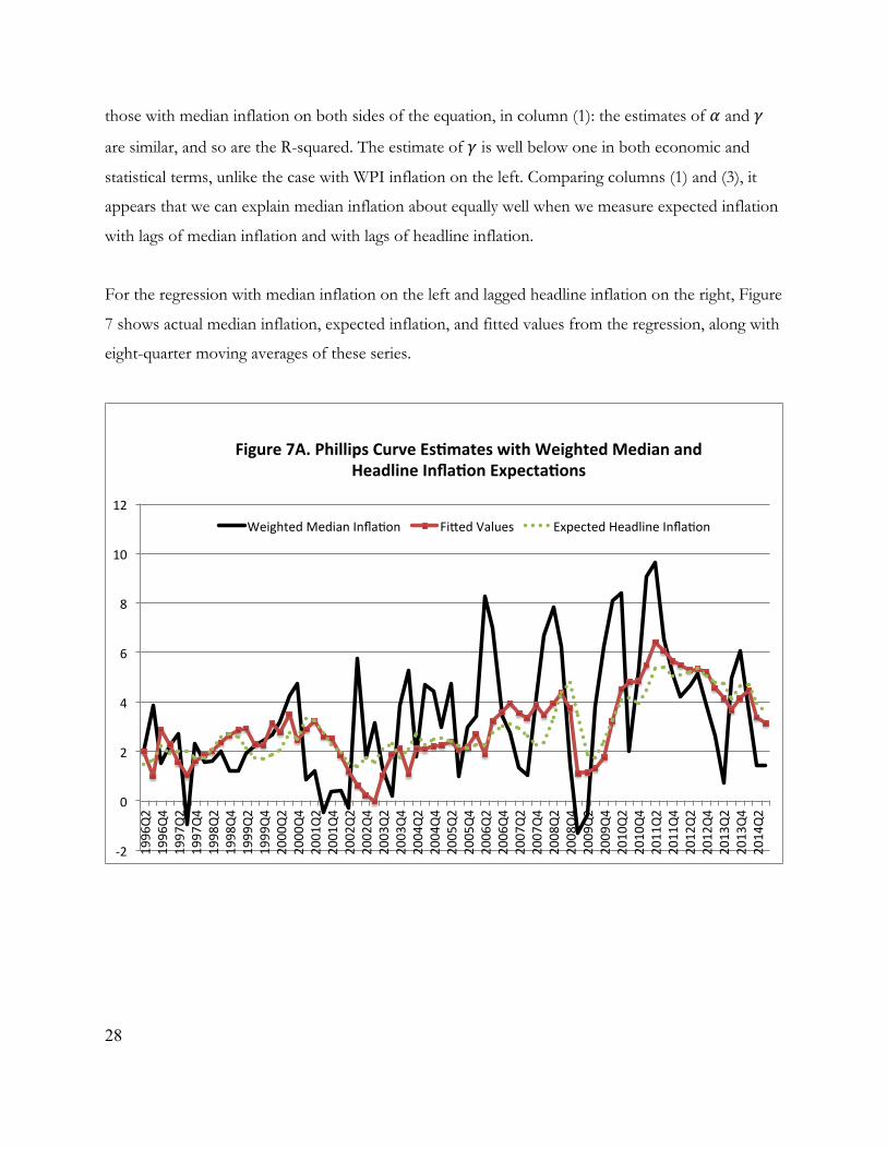
For the regression with median inflation on the left and lagged headline inflation on the right, Figure

7 shows actual median inflation, expected inflation, and fitted values from the regression, along with

eight-quarter moving averages of these series.

!2#

0#

2#

4#

6#

8#

10#

12#

1996Q2#

1996Q4#

1997Q2#

1997Q4#

1998Q2#

1998Q4#

1999Q2#

1999Q4#

2000Q2#

2000Q4#

2001Q2#

2001Q4#

2002Q2#

2002Q4#

2003Q2#

2003Q4#

2004Q2#

2004Q4#

2005Q2#

2005Q4#

2006Q2#

2006Q4#

2007Q2#

2007Q4#

2008Q2#

2008Q4#

2009Q2#

2009Q4#

2010Q2#

2010Q4#

2011Q2#

2011Q4#

2012Q2#

2012Q4#

2013Q2#

2013Q4#

2014Q2#

Figure'7A.'Phillips'Curve'Es3mates'with'Weighted'Median'and'Headline'Infla3on'Expecta3ons'

Weighted#Median#Infla:on# Fi=ed#Values# Expected#Headline#Infla:on#

29

In column (4), we investigate whether lagged headline or lagged core inflation belongs on the right

side of the Phillips curve by including both in a horserace.

Here, we assume that an exponential average of past median inflation has a weight of 𝛽 in

determining expectations, and an average of past WPIs has a weight of 1− 𝛽. Notice that we

constrain the exponential coefficient 𝛾 to be the same in the two averages; the qualitative results are

similar if we estimate two different 𝛾s.

Our estimates for this specification are imprecise. This reflects the fact that median inflation and

WPI inflation have similar medium-term movements; thus, while these two inflation rates have only

a modest correlation at the quarterly frequency, slow moving averages of the two are strongly

correlated, so there is a problem of multicollinearity.

Nonetheless, we can see where the estimates point. The key result is that the estimate of the weight

0"

1"

2"

3"

4"

5"

6"

7"

8"

1996Q2"

1996Q4"

1997Q2"

1997Q4"

1998Q2"

1998Q4"

1999Q2"

1999Q4"

2000Q2"

2000Q4"

2001Q2"

2001Q4"

2002Q2"

2002Q4"

2003Q2"

2003Q4"

2004Q2"

2004Q4"

2005Q2"

2005Q4"

2006Q2"

2006Q4"

2007Q2"

2007Q4"

2008Q2"

2008Q4"

2009Q2"

2009Q4"

2010Q2"

2010Q4"

2011Q2"

2011Q4"

2012Q2"

2012Q4"

2013Q2"

2013Q4"

2014Q2"

Figure'7B.'Phillips'Curve'Es3mates'with'Weighted'Median'and'Headline'Infla3on'Expecta3ons:'8Dquarter'Moving'Avaerages'

Weighted"Median"Infla9on" Fi<ed"Values" Expected"Headline"Infla9on"

30

𝛽 on past median inflation is 0.26 with a standard error of 0.28. A two-standard error confidence

interval is [-0.30, 0.82]. While this range is wide, we can reject the hypothesis that 𝛽 is one--that only

past median inflation affects expectations--and cannot reject the hypothesis that 𝛽 is zero--that only

past headline inflation matters. The estimate of 𝛾 exceeds one, but this may simply reflect sampling

error, as a two-standard-error band extends down to 0.88.

In sum, the data suggest that past headline inflation has a substantial effect on expected inflation, so,

as in the pre-Volcker United States, a supply shock that raises inflation in one quarter can have a

persistent effect on core inflation through its effect on expectations.

Food and Energy Again

Throughout our analysis, we have examined the effects of changes in the relative price of food and

energy, measured by food and energy inflation minus aggregate WPI inflation. This relative price

changes when are there events in the real economy affecting the supply and demand for food and

energy. In our framework, large shocks of this nature influence aggregate inflation; again, the

underlying theory is that of Ball and Mankiw (1995), in which large shocks have disproportionately

large effects on inflation because they trigger adjustment of nominal prices that might otherwise be

sticky.

In India, economists debate the reasons for rises and falls in food prices. In particular, some cite

supply side factors such as low and stagnant production of food, and others emphasize demand

factors such as shifting diets. We do not take a position in this debate, and our results do not shed

light on it. In our framework, a large shock to food and fuel prices has the same effect on the price-

change distribution, and hence on inflation, regardless of its underlying demand or supply causes.

Much of the literature on India’s inflation investigates the interactions of food inflation-the change

in the nominal price of food - with non-food inflation or aggregate inflation. In our view, such

empirical analyses do not have a clear interpretation. A change in food prices is an event in the real

economy only to the extent it differs from aggregate inflation; otherwise, it is simply part of the

inflationary process affecting all prices.

31

In an accounting sense, one can explain aggregate inflation with an equation that includes different

components of inflation. If all the components are included, one obtains an equation with an R

squared of one, and coefficients on each component equal to its share in the aggregate price index.

Even if only one or a few components are included in the equation, they can appear to have high

explanatory power if movements in aggregate inflation cause correlated movements in the inflation

rates for many industries.

A similar point applies to studies that regress aggregate inflation or non-food inflation on lags of

food inflation or other sectoral inflation rates. In these equations, lagged food inflation may simply

be a proxy for lagged aggregate inflation if there is a strong common component in the inflation

rates of different sectors. Whether a measure of food inflation is contemporaneous or lagged, it can

tell us something about the determinants of inflation only if is measured relative to aggregate

inflation.

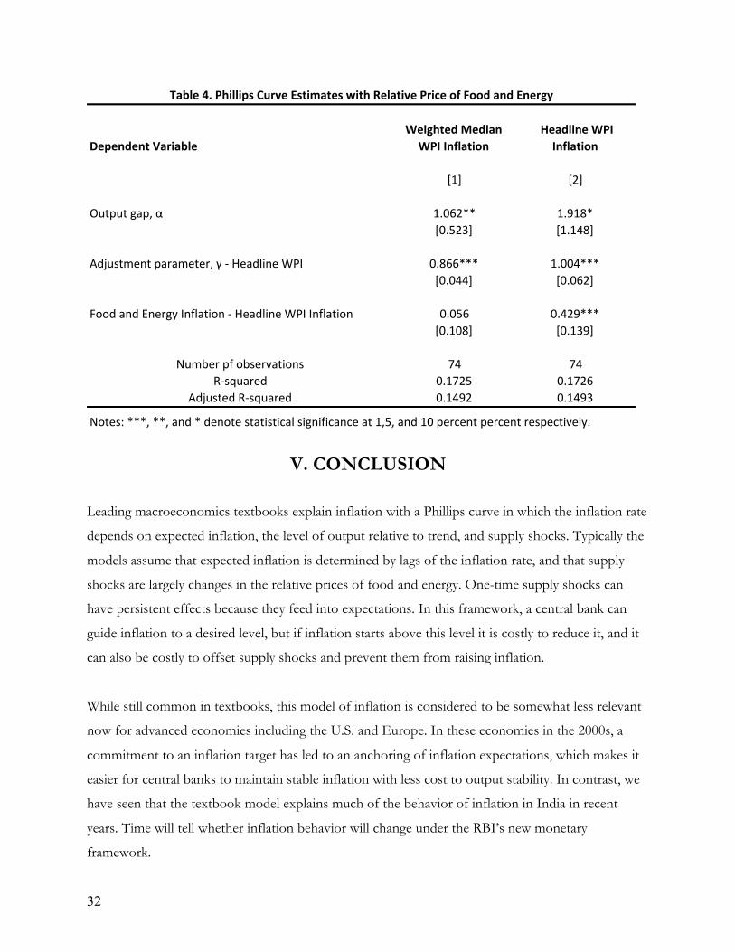
In Table 4, we include the change in the relative price of food and energy, measured by food and

energy inflation minus headline inflation, in the estimation of the Phillips curve. The dependent

variables are weighted median and headline inflation in columns [1] and [2] respectively. Not

surprisingly, as shown in column [1], the relative price of food and energy does not have a significant

effect on weighted median inflation, which is stripped of volatile components. Column [2] shows

that the relative price of food and energy does have a statistically significant effect on headline

inflation. The estimated coefficient is 0.43, and the standard error is 0.14. The results support the

earlier evidence that changes in the relative price of food and energy, which predominantly

constitute the right tail of the distribution of price changes, strongly influence aggregate inflation.

32

V. CONCLUSION

Leading macroeconomics textbooks explain inflation with a Phillips curve in which the inflation rate

depends on expected inflation, the level of output relative to trend, and supply shocks. Typically the

models assume that expected inflation is determined by lags of the inflation rate, and that supply

shocks are largely changes in the relative prices of food and energy. One-time supply shocks can

have persistent effects because they feed into expectations. In this framework, a central bank can

guide inflation to a desired level, but if inflation starts above this level it is costly to reduce it, and it

can also be costly to offset supply shocks and prevent them from raising inflation.

While still common in textbooks, this model of inflation is considered to be somewhat less relevant

now for advanced economies including the U.S. and Europe. In these economies in the 2000s, a

commitment to an inflation target has led to an anchoring of inflation expectations, which makes it

easier for central banks to maintain stable inflation with less cost to output stability. In contrast, we

have seen that the textbook model explains much of the behavior of inflation in India in recent

years. Time will tell whether inflation behavior will change under the RBI’s new monetary

framework.

Dependent'VariableWeighted'Median'WPI'Inflation

'Headline'WPI'Inflation

[1] [2]

Output)gap,)α 1.062** 1.918*[0.523] [1.148]

Adjustment)parameter,)γ)@)Headline)WPI 0.866*** 1.004***[0.044] [0.062]

Food)and)Energy)Inflation)@)Headline)WPI)Inflation 0.056 0.429***[0.108] [0.139]

Number)pf)observations 74 74R@squared 0.1725 0.1726

Adjusted)R@squared 0.1492 0.1493

Table'4.'Phillips'Curve'Estimates'with'Relative'Price'of'Food'and'Energy

Notes:)***,)**,)and)*)denote)statistical)significance)at)1,5,)and)10)percent)percent)respectively.)

33

REFERENCES Balakrishna, P. “Pricing and Inflation in India”. Oxford University Press Delhi. Ball, Laurence, and N. Gregory Mankiw, ‘‘Relative-Price Changes as Aggregate Supply Shocks,’’ Quarterly Journal of Economics 110 (February 1995), 161–193. Laurence Ball & Sandeep Mazumder, 2014. "A Phillips Curve with Anchored Expectations and Short-Term Unemployment," NBER Working Papers 20715, National Bureau of Economic Research, Inc. Ball, Laurence and Sandeep Mazumder, 2011, "Inflation Dynamics and the Great Recession," Brookings Papers on Economic Activity, Economic Studies Program, The Brookings Institution, vol. 42(1 (Spring), pages 337-405. Bernanke, Ben, Thomas Laubach, Frederic Mishkin, and Adam Posen (1999). Inflation Targeting: Lessons from the International Experience. Princeton N.J.: Princeton University Press. Bhattacharya, B. B., and M. Lodh (1990): "Inflation in India: An Analytical Survey," Artha Vijnana, 32, 25-68. Bhalla, Surjit, 2014a, ‘Where monetary policy is irrelevant’, Indian Express, September 13, 2014. Bhalla, Surjit, 2014b, ‘RBI, we have a problem’, September 20, 2014. Brahmananda, P., and G. Nagaraju (2002), "Inflation and Growth in the World: Some Simple Empirics, 1970–99," Macroeconomics and monetary policy: Issues for a reforming economy, Oxford University Press, New Delhi, 43-66. Callen and Chang (1999) Chatterji, R. (1989): The Behaviour of Industrial Prices in India. Oxford University Press Delhi. Das, S. (2003): "Modelling Money, Price and Output in India: A Vector Autoregressive and Moving Average (VARMA) Approach," Applied Economics, 35, 1219-1225. Das, Abhiman (2014), “Role of Inflation Expectation in Estimating a Phillips Curve for India”, mimeo. Dholakia, R.H. (1990), "Extended Phillips Curve for the Indian Economy," Indian Economic Journal, 38, 69-78. Dua, P., and U. Gaur (2009): "Determination of Inflation in an Open Economy Phillips Curve Framework: The Case of Developed and Developing Asian Countries," Centre for Development Economics Working Paper. Economic Survey, 2013, Ministry of Finance, Government of India.

34

Gokarn, Sunir (2011) “The price of protein”, Macroeconomics and Finance in Emerging Market Economies, 4:2, 327-335, DOI: 10.1080/17520843.2011.593908. Gokarn, Subir (1997), “Economic reforms and relative price movements in India: a 'supply shock' approach”, The Journal of International Trade & Economic Development, 1997, vol. 6, issue 2, pages 299-324. Gordon, R. (1982): “Inflation, Flexible Exchange Rates, and the Natural Rate of Unemployment,” in Workers, Jobs, and Inflation, ed. by M. Baily, The Brookings Institution, 89–158. ——— (1990): “U.S. Inflation, Labor’s Share, and the Natural Rate of Unemployment,” in Economics of Wage Determination, ed. by H. Koenig, Berlin: Springer-Verlag. ——— (2011): “The History of the Phillips Curve: Consensus and Bifurcation,” Economica, 78, 10–50. Kapur, M. (2013): "Revisiting the Phillips Curve for India and Inflation Forecasting," Journal of Asian Economics, 25, 17-27. Kotia, Ananya, 2013,“An Unobserved Philips Curve for India” . Available at SSRN: http://ssrn.com/abstract=2315995 or http://dx.doi.org/10.2139/ssrn.2315995. Mazumder, S. (2011): "The Stability of the Phillips Curve in India: Does the Lucas Critique Apply?," Journal of Asian Economics, 22, 528-539. Lahiri, Amartya, 2014, “Don’t blame MSP for inflation”, Indian Express, October 7, 2014. Mishra, Prachi, and Devesh Roy, “Explaining Inflation in India: The Role of Food Prices”, Brookings-NCAER India Policy Forum. Volume 8, 2011-12. Mishra, Prachi, 2013, “Has India's Growth Story Withered?” Economic and Political Weekly, April 13, 2013 Mitra, Pratik, Dipankar Biswas, and Anirban Sanyal (2015), “Estimating Sacrifice Ratio for Indian Economy – A Time Varying Perspective”, RBI Working Paper Series 1. Nachane, D. and R. Lakshmi, (2002): "Dynamics of Inflation in India-a P-Star Approach," Applied Economics, 34, 101-110. Patra, M.D.., and M. Kapur (2012): "A Monetary Policy Model for India," Macroeconomics and Finance in Emerging Market Economies, 5, 18-41. Rajan, Raghuram, “Fighting Inflation”, Inaugural speech, Governor, Reserve Bank of India at FIMMDA-PDAI Annual Conference 2014, on February 26, 2014 at Mumbai. Rangarajan, C. (1983): "Conflict between Employment and Inflation," in Employment Policy in a Developing Country-a Case Study, ed. by A. Robinson: Macmillan. Rangarajan, C., and R. Arif (1990): "Money, Output and Prices: A Macro Econometric Model," Economic and Political Weekly, 837-852.

35

Srinivasan, N., Mahambare, V., and M. Ramachandra (2006): "Modeling Inflation in India: Critique of the Structuralist Approach," Journal of Quantitative Economics, New Series 4, 45-58. Stock, J. and M. Watson (2007): “Why Has U.S. Inflation Become Harder to Forecast?” Journal of Money, Credit and Banking, 39, 3–33. ——— (2008): “Phillips Curve Inflation Forecasts,” NBER Working Paper, 14322. ——— (2010): “Modeling Inflation After the Crisis,” NBER Working Paper, 16488.

Virmani, A. (2004): "Estimating Output Gap for the Indian Economy: Comparing Results from Unobserved-Components Models and the Hodrick-Prescott Filter," Indian Institute of Management Ahmedabad, Research and Publication Department.

36

APPENDIX

Appendix 1. Data Details

Median Inflation in 2004Q2

There is a discontinuity in the monthly series on industry price levels that we use to calculate

weighted median inflation. A new series begins for each industry in April 2004, and it is not

comparable to the earlier data. In addition, 20 industries are added, bringing the total number from

61 to 81. For our quarterly analysis, this break in the data makes it difficult to measure median

inflation for 2004Q2.

We approximate median inflation in 2004Q2 as follows. We use the 61 industries that exist both

before and after the quarter. For each industry, we assume that the gross monthly inflation rate for

April 2004 is the geometric average of the gross inflation rates for February, March, May, and June

2004. With this industry inflation rate in hand, we can compute a consistent series of monthly price

levels that spans April 2004. We aggregate monthly price levels to get quarterly price levels for each

industry; then calculate quarterly inflation rates; and then calculate weighted median inflation for the

61 industries.

Splicing Methodology for GDP Series

We compute a consistent series for real GDP (before seasonal adjustment) using two series with

base years of 1999-2000 and 2004-2005. Essentially, we project the 2004-05 series (which starts in

2004Q2) backwards using the growth rates from the 1999-2000 series. Specifically:

For observations starting in 2004Q2, we use the output levels from the 2004-2005 base year series. We work backward to get output in 2004Q1, 2003Q4, and so on, using the formula

𝑦! = !!!!

(!!!!!! )

37

where 𝑦! and 𝑦!!! are output levels in quarters 𝑡 and 𝑡 + 4, and 𝑔!!! is the growth rate of output

from 𝑡 to 𝑡 + 4. For all the observations for 2004Q1 and earlier, 𝑔!!! is computed from the output

series for base year 1999-2000. For observations from 2004Q1 back to 2003Q2, 𝑦!!! is from the

output series with 2004-2005 base year. For observations for 2003Q1 and earlier, 𝑦!!! comes from

an earlier step in our backward iteration.

Appendix 2: Details of Estimation

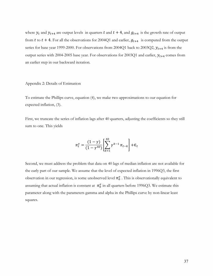
To estimate the Phillips curve, equation (4), we make two approximations to our equation for

expected inflation, (3).

First, we truncate the series of inflation lags after 40 quarters, adjusting the coefficients so they still

sum to one. This yields

𝜋!! =(1− 𝛾)(1− 𝛾!") 𝛾!!!

!"

!!!

𝜋!!! +∈!

Second, we must address the problem that data on 40 lags of median inflation are not available for

the early part of our sample. We assume that the level of expected inflation in 1996Q3, the first

observation in our regression, is some unobserved level 𝜋!! . This is observationally equivalent to

assuming that actual inflation is constant at 𝜋!! in all quarters before 1996Q3. We estimate this

parameter along with the parameters gamma and alpha in the Phillips curve by non-linear least

squares.