Understanding intra-urban trip patterns from taxi ...Received: 31 August 2011/Accepted: 5 March 2012/Published online: 21 March 2012 Springer-Verlag 2012 Abstract Intra-urban human

ORI GIN AL ARTICLE

Understanding intra-urban trip patternsfrom taxi trajectory data

Yu Liu • Chaogui Kang • Song Gao • Yu Xiao •

Yuan Tian

Received: 31 August 2011 / Accepted: 5 March 2012 / Published online: 21 March 2012

� Springer-Verlag 2012

Abstract Intra-urban human mobility is investigated by means of taxi trajectory

data that are collected in Shanghai, China, where taxis play an important role in

urban transportation. From the taxi trajectories, approximately 1.5 million trips of

anonymous customers are extracted on seven consecutive days. The globally spatio-

temporal patterns of trips exhibit a significant daily regularity. Since each trip can be

viewed as a displacement in the random walk model, the distributions of the dis-

tance and direction of the extracted trips are investigated in this research. The

direction distribution shows an NEE–SWW-dominant direction, and the distance

distribution can be well fitted by an exponentially truncated power law, with the

scaling exponent b = 1.2 ± 0.15. The observed patterns are attributed to the geo-

graphical heterogeneity of the study area, which makes the spatial distribution of

trajectory stops to be non-uniform. We thus construct a model that integrates both

the geographical heterogeneity and distance decay effect, to interpret the observed

patterns. Our Monte Carlo simulation results closely match to the observed patterns

and thus validate the proposed model. According to the proposed model, in a single-

core urban area, the geographical heterogeneity and distance decay effect improve

each other when influencing human mobility patterns. Geographical heterogeneity

leads to a faster observed decay, and the distance decay effect makes the spatial

distribution of trips more concentrated.

Keywords Intra-urban human mobility � Taxi trajectory � Geographical

heterogeneity � Distance decay � Monte Carlo simulation

JEL Classification C15 � R40

Y. Liu (&) � C. Kang � S. Gao � Y. Xiao � Y. Tian

Institute of Remote Sensing and Geographical Information Systems, Beijing 100871, China

e-mail: [email protected]

123

J Geogr Syst (2012) 14:463–483

DOI 10.1007/s10109-012-0166-z

1 Introduction

Human mobility has become a hot research topic recently, since the wide use of

location-aware devices such as GPS (global positioning system) receivers and

mobile phones offers great convenience for collecting large volumes of individual

trajectory data (Gonzalez et al. 2008; Jiang et al. 2009; Rhee et al. 2008; Song et al.

2010a, b; Yuan et al. 2012). Cities are concentrated areas of human activities, and

thus, intra-urban motion is a dominant part of life for citizens. Identifying patterns

of intra-urban human mobility will help us understand urban dynamics and reveal

the driving social factors, such as gender and occupation (Sang et al. 2011).

Currently, location-aware devices are widely applied in urban studies (Chowell

et al. 2003; Phithakkitnukoon et al. 2010; Ratti et al. 2006; Shoval 2008). In terms

of mobile data, Ahas et al. (2010) investigated the movement patterns of suburban

commuters of Tallinn, Estonia, using mobile positioning data and identified a

remarkable temporal rhythm of respondents’ locations. The motion of mobile users

leads to varying traffic intensities of corresponding base stations, which can be

measured using Erlang values.1 Ratti et al. (2006) mapped the dynamics of urban

activities in the metropolitan area of Milan, Italy, using the Erlang values of cell

phone stations. Sevtsuk and Ratti (2010) also adopted Erlang measures in Rome,

Italy, and found significant temporal regularity in human mobility. A similar study

based on principal component analysis was conducted by Sun et al. (2011) using

data collected in Shenzhen, China.

In addition to mobile data, bank notes (Brockmann et al. 2006), travel bugs

(Brockmann and Theis 2008), and check-ins in location sharing services (Cheng et al.

2011) can also be used for understanding human mobility patterns. Recently, GPS-

enabled floating cars2 have provided an alternative approach to gathering large

volumes of individual trajectories and studying individuals’ behaviors and urban

dynamics (Jiang et al. 2009; Liu et al. 2010; Li et al. 2011; Qi et al. 2011; Zheng et al.

2011). The floating car technique has been adopted by intelligent transportation

systems (ITSs) to collect traffic information in recent years (Dai et al. 2003; Kuhne

et al. 2003; Lu et al. 2008; Tong et al. 2009). Each floating car periodically records its

positional information, which is obtained using a GPS receiver, and sends such

information to the data center. Using the collected data from a large number of floating

cars, the real-time traffic status of a city can be estimated and assessed. In practice,

floating cars are often served by taxis in many cities (Li et al. 2011), and thus, it is

convenient to collect human mobility data. For instance, Jiang et al. (2009) analyzed

trajectories of individuals, which were obtained from taxis of four cities in Sweden,

and argued that the mobility pattern is determined by the street layout.

A number of mobility models have been proposed, including random way point,

random direction, Brownian motion, random walk, and obstacle model for describing

human movement (Lee et al. 2009). Much research has shown that the human mobility

1 The traffic measured in Erlang values represents the average number of concurrent calls carried by a

mobile phone tower. The motion of mobile users leads to varying traffic intensities of corresponding base

stations, which can be measured using Erlang values.2 A number of types of floating car data, such as cellular network-based data and electronic toll-based

data, are available at present. This research uses GPS-based floating car data.

464 Y. Liu et al.

123

patterns can be modeled using Levy flight or truncated Levy flight (Brockmann et al.

2006; Jiang et al. 2009; Rhee et al. 2008). A Levy flight is a specific random walk

model that satisfies the following two conditions: (1) the step lengths follow a power

law, or a truncated power law for truncated Levy flights, and (2) the angle distribution

is uniform. The power law distribution of step lengths indicates distance decay, which

widely exists in geographical phenomena. For example, Lu (2003) found a power law

distance decay effect in criminals’ journey-after-auto-theft in Buffalo, USA. Many

geographical models, such as the gravity model, are constructed directly based on

power law distance decay. In practice, it is difficult to collect sufficient data to examine

whether the trajectory of a particular individual follows the Levy flight model. Hence,

the examinations are often conducted using data sets that consist of large numbers of

individual trajectories, and thus, the statistics exhibit a convolution of population

heterogeneity and individual motion (Gonzalez et al. 2008).

A metropolitan area is a region where human activities are highly concentrated,

and thus forms a relatively complete unit for analyzing human mobility patterns.

Will the intra-urban human mobility patterns be different from the patterns reported

in existing literature? How to interpret the observed patterns by taking into account

geographical impacts? This research adopts the taxi trajectories of Shanghai, China,

to address the two questions. Taxis occupy a large proportion of urban traffic

services in Shanghai, and the underlying patterns in the taxi trajectories thus reflect

the characteristics of human mobility. About 1.5 million trips of anonymous

customers are extracted from the taxi trajectory data. Each trip is represented by a

vector h(xi1, yi1, ti1), (xi2, yi2, ti2)i, where (xi1, yi1) and (xi2, yi2) denote positions

where a customer was picked up and dropped off, and ti2 and ti2 are the pick-up time

and drop-off time, respectively. In general, one trip is associated with a specific

purpose, so that one can stay at both (xi1, yi1) and (xi2, yi2) for a period of time and

continuously move between (xi1, yi1) and (xi2, yi2). Hence, such a trip can be viewed

as a displacement in the random walk model of an individual.

In this research, the distance and direction distributions of intra-urban trips are

focused on. The trip distances follow the exponentially truncated power law distribution,

which is consistent with the findings of Brockmann et al. (2006) and Gonzalez et al.

(2008). The direction distribution, however, is not uniform. We conjecture that the

identified patterns are influenced by geographical heterogeneity; that is, the probability

that a point serves as a potential stop in a trajectory varies in geographical space. Monte

Carlo simulations reproduce the observed patterns well and thus confirm the conjecture.

Compared with existing studies, this research highlights the impact of geographical

heterogeneity on human mobility patterns and points out that the observed decay in

distance distributions should be attributed to two aspects: heterogeneous geographical

space and the inherent distance decay effect associated with spatial behavior.

Additionally, there is a reciprocity effect between these two aspects.

2 Data

Shanghai is the most populous city in China. Taxis play an important role in the

urban transportation of Shanghai. At the end of 2009, 149 companies possessed

Understanding intra-urban trip patterns 465

123

approximately 47,000 taxis in Shanghai Municipality. If we consider only the urban

area, there are 130 companies and 43,000 taxis. In 2009, these taxis carried about

three million passengers each day, occupying more than 20 % of the intra-urban

travel within Shanghai.3 Many taxi companies have their vehicles equipped with

GPSs to monitor the operation of each taxi. Meanwhile, the urban government can

use the taxis that are equipped with GPS receivers as ‘‘floating’’ cars to obtain the

status of real-time traffic.

In this research, the data set records more than 6,600 floating cars of an

anonymous taxi company of Shanghai. The data set spans seven consecutive days,

from June 1, 2009, to June 7, 2009. For each taxicab, information on its position,

velocity, and whether customers are being transported is automatically collected

approximately every 10 s. Theoretically, there should be approximately 55 million

records each day. However, the actual data volume, including about 47 million

records, is slightly less because some taxi drivers could shut down their GPS

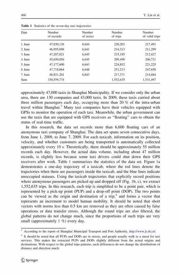
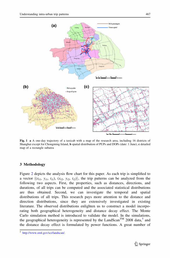
receivers after work. Table 1 summarizes the statistics of the data set. Figure 1a

demonstrates a one-day trajectory of a taxicab, where the red lines denote the

trajectories when there are passengers inside the taxicab, and the blue lines indicate

unoccupied statuses. Using the taxicab trajectories that explicitly record positions

where anonymous passengers are picked up and dropped off (Fig. 1b, c), we extract

1,552,635 trips. In this research, each trip is simplified to be a point pair, which is

represented by a pick-up point (PUP) and a drop-off point (DOP). The two points

can be viewed as the origin and destination of a trip,4 and forms a vector that

represents an increment to model human mobility. It should be noted that short

vectors with norms less than 0.5 km are removed as they are often caused by false

operations or data transfer errors. Although the round trips are also filtered, the

global patterns do not change much, since the proportions of such trips are very

small (approximately 1 %) every day.

Table 1 Statistics of the seven-day taxi trajectories

Date Number

of records

Number

of taxies

Number

of trips

Number

of valid trips

1 June 47,030,136 6,644 220,203 217,491

2 June 46,955,696 6,641 214,313 211,299

3 June 47,207,021 6,645 215,185 212,427

4 June 45,650,056 6,645 209,498 206,721

5 June 47,177,600 6,643 224,852 221,225

6 June 47,718,064 6,648 251,213 247,650

7 June 48,821,201 6,643 217,371 214,684

Sum 330,559,774 1,552,635 1,531,497

3 According to the report of Shanghai Municipal Transport and Port Authority, http://www.jt.sh.cn/.4 It should be noted that all PUPs and DOPs are in streets, and people usually walk to a street for taxi

services. This makes the extracted PUPs and DOPs slightly different from the actual origins and

destinations. With respect to the global trips patterns, such differences do not change the distributions of

distance and direction much.

466 Y. Liu et al.

123

http://www.jt.sh.cn/

3 Methodology

Figure 2 depicts the analysis flow chart for this paper. As each trip is simplified to

a vector h(xi1, yi1, ti1), (xi2, yi2, ti2)i, the trip patterns can be analyzed from the

following two aspects. First, the properties, such as distances, directions, and

durations, of all trips can be computed and the associated statistical distributions

are thus obtained. Second, we can investigate the temporal and spatial

distributions of all trips. This research pays more attention to the distance and

direction distributions, since they are extensively investigated in existing

literature. The observed distributions enlighten us to construct a model incorpo-

rating both geographical heterogeneity and distance decay effect. The Monte

Carlo simulation method is introduced to validate the model. In the simulations,

the geographical heterogeneity is represented by the LandScanTM 2008 data,5 and

the distance decay effect is formulated by power functions. A great number of

Fig. 1 a A one-day trajectory of a taxicab with a map of the research area, including 16 districts ofShanghai except for Chongming Island, b spatial distribution of PUPs and DOPs (date: 1 June), c detailedmap of a rectangle subarea

5 http://www.ornl.gov/sci/landscan/.


123

http://www.ornl.gov/sci/landscan/

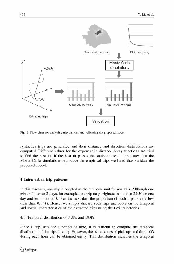
synthetics trips are generated and their distance and direction distributions are

computed. Different values for the exponent in distance decay functions are tried

to find the best fit. If the best fit passes the statistical test, it indicates that the

Monte Carlo simulations reproduce the empirical trips well and thus validate the

proposed model.

4 Intra-urban trip patterns

In this research, one day is adopted as the temporal unit for analysis. Although one

trip could cover 2 days, for example, one trip may originate in a taxi at 23:50 on one

day and terminate at 0:15 of the next day, the proportion of such trips is very low

(less than 0.1 %). Hence, we simply discard such trips and focus on the temporal

and spatial characteristics of the extracted trips using the taxi trajectories.

4.1 Temporal distribution of PUPs and DOPs

Since a trip lasts for a period of time, it is difficult to compute the temporal

distribution of the trips directly. However, the occurrences of pick-ups and drop-offs

during each hour can be obtained easily. This distribution indicates the temporal

Fig. 2 Flow chart for analyzing trip patterns and validating the proposed model

468 Y. Liu et al.

123

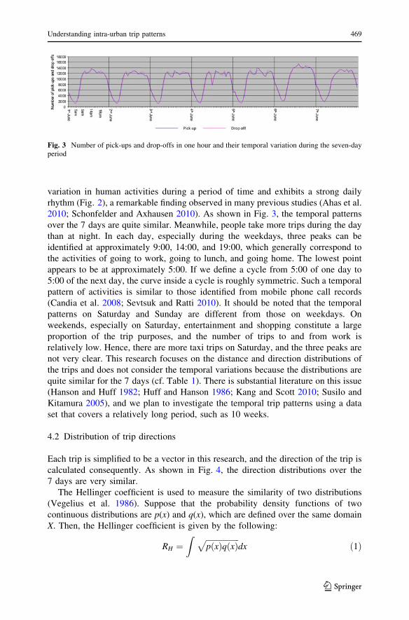
variation in human activities during a period of time and exhibits a strong daily

rhythm (Fig. 2), a remarkable finding observed in many previous studies (Ahas et al.

2010; Schonfelder and Axhausen 2010). As shown in Fig. 3, the temporal patterns

over the 7 days are quite similar. Meanwhile, people take more trips during the day

than at night. In each day, especially during the weekdays, three peaks can be

identified at approximately 9:00, 14:00, and 19:00, which generally correspond to

the activities of going to work, going to lunch, and going home. The lowest point

appears to be at approximately 5:00. If we define a cycle from 5:00 of one day to

5:00 of the next day, the curve inside a cycle is roughly symmetric. Such a temporal

pattern of activities is similar to those identified from mobile phone call records

(Candia et al. 2008; Sevtsuk and Ratti 2010). It should be noted that the temporal

patterns on Saturday and Sunday are different from those on weekdays. On

weekends, especially on Saturday, entertainment and shopping constitute a large

proportion of the trip purposes, and the number of trips to and from work is

relatively low. Hence, there are more taxi trips on Saturday, and the three peaks are

not very clear. This research focuses on the distance and direction distributions of

the trips and does not consider the temporal variations because the distributions are

quite similar for the 7 days (cf. Table 1). There is substantial literature on this issue

(Hanson and Huff 1982; Huff and Hanson 1986; Kang and Scott 2010; Susilo and

Kitamura 2005), and we plan to investigate the temporal trip patterns using a data

set that covers a relatively long period, such as 10 weeks.

4.2 Distribution of trip directions

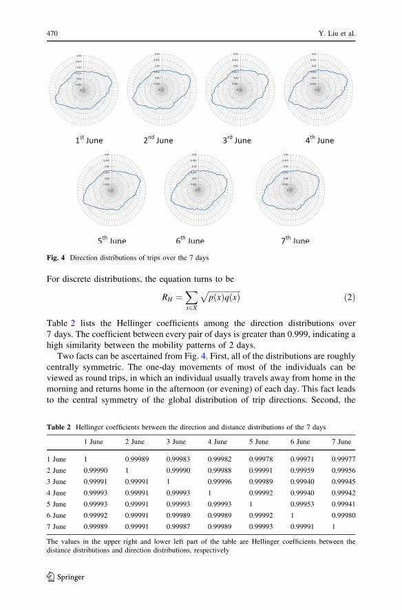
Each trip is simplified to be a vector in this research, and the direction of the trip is

calculated consequently. As shown in Fig. 4, the direction distributions over the

7 days are very similar.

The Hellinger coefficient is used to measure the similarity of two distributions

(Vegelius et al. 1986). Suppose that the probability density functions of two

continuous distributions are p(x) and q(x), which are defined over the same domain

X. Then, the Hellinger coefficient is given by the following:

RH ¼Z ffiffiffiffiffiffiffiffiffiffiffiffiffiffiffiffiffi

pðxÞqðxÞp

dx ð1Þ

Fig. 3 Number of pick-ups and drop-offs in one hour and their temporal variation during the seven-dayperiod


123

For discrete distributions, the equation turns to be

RH ¼Xx2X

ffiffiffiffiffiffiffiffiffiffiffiffiffiffiffiffiffipðxÞqðxÞ

pð2Þ

Table 2 lists the Hellinger coefficients among the direction distributions over

7 days. The coefficient between every pair of days is greater than 0.999, indicating a

high similarity between the mobility patterns of 2 days.

Two facts can be ascertained from Fig. 4. First, all of the distributions are roughly

centrally symmetric. The one-day movements of most of the individuals can be

viewed as round trips, in which an individual usually travels away from home in the

morning and returns home in the afternoon (or evening) of each day. This fact leads

to the central symmetry of the global distribution of trip directions. Second, the

Fig. 4 Direction distributions of trips over the 7 days

Table 2 Hellinger coefficients between the direction and distance distributions of the 7 days

1 June 2 June 3 June 4 June 5 June 6 June 7 June

1 June 1 0.99989 0.99983 0.99982 0.99978 0.99971 0.99977

2 June 0.99990 1 0.99990 0.99988 0.99991 0.99959 0.99956

3 June 0.99991 0.99991 1 0.99996 0.99989 0.99940 0.99945

4 June 0.99993 0.99991 0.99993 1 0.99992 0.99940 0.99942

5 June 0.99993 0.99991 0.99993 0.99993 1 0.99953 0.99941

6 June 0.99992 0.99991 0.99989 0.99989 0.99992 1 0.99980

7 June 0.99989 0.99991 0.99987 0.99989 0.99993 0.99991 1

The values in the upper right and lower left part of the table are Hellinger coefficients between the

distance distributions and direction distributions, respectively

470 Y. Liu et al.

123

angle distributions are not uniform, with two major directions: northeast east (NEE)

and southwest west (SWW).

4.3 Distribution of trip distances

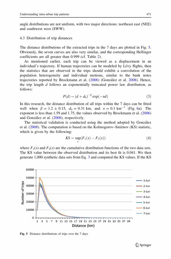
The distance distributions of the extracted trips in the 7 days are plotted in Fig. 5.

Obviously, the seven curves are also very similar, and the corresponding Hellinger

coefficients are all greater than 0.999 (cf. Table 2).

As mentioned earlier, each trip can be viewed as a displacement in an

individual’s trajectory. If human trajectories can be modeled by Levy flights, then

the statistics that are observed in the trips should exhibit a convolution of the

population heterogeneity and individual motions, similar to the bank notes

trajectories reported by Brockmann et al. (2006) (Gonzalez et al. 2008). Hence,

the trip length d follows an exponentially truncated power law distribution, as

follows:

PðdÞ� ðd þ d0Þ�bexpð�adÞ ð3Þ

In this research, the distance distribution of all trips within the 7 days can be fitted

well when b = 1.2 ± 0.15, d0 = 0.31 km, and a = 0.1 km-1 (Fig. 6a). The

exponent is less than 1.59 and 1.75, the values observed by Brockmann et al. (2006)

and Gonzalez et al. (2008), respectively.

The statistical validation is conducted using the method adopted by Gonzalez

et al. (2008). The computation is based on the Kolmogorov–Smirnov (KS) statistic,

which is given by the following:

KS ¼ supxðF1ðxÞ � F2ðxÞÞ ð4Þ

where F1(x) and F2(x) are the cumulative distribution functions of the two data sets.

The KS value between the observed distribution and its best fit is 0.041. We then

generate 1,000 synthetic data sets from Eq. 3 and computed the KS values. If the KS

Fig. 5 Distance distributions of trips over the 7 days


123

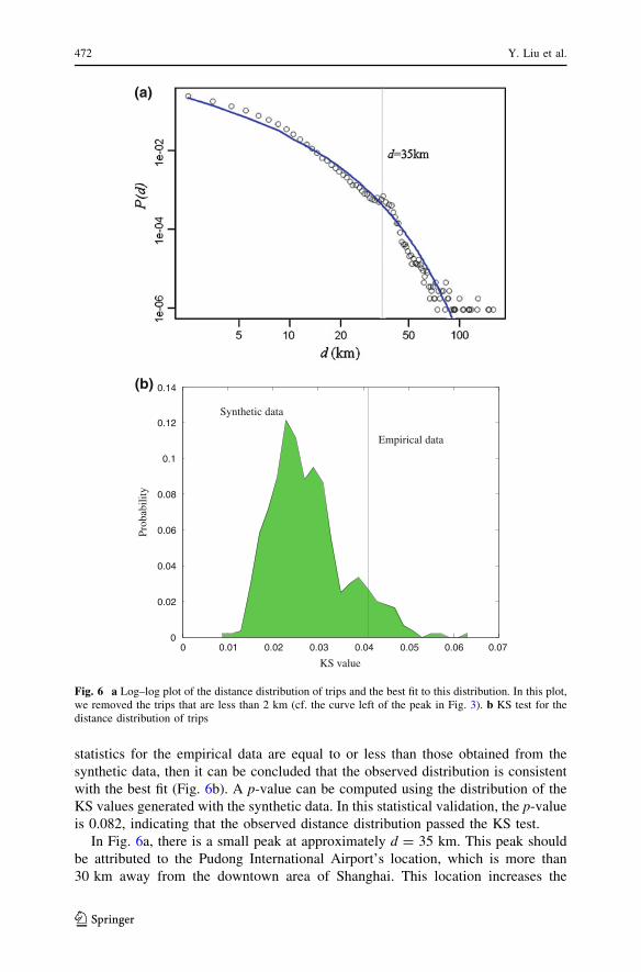
statistics for the empirical data are equal to or less than those obtained from the

synthetic data, then it can be concluded that the observed distribution is consistent

with the best fit (Fig. 6b). A p-value can be computed using the distribution of the

KS values generated with the synthetic data. In this statistical validation, the p-value

is 0.082, indicating that the observed distance distribution passed the KS test.

In Fig. 6a, there is a small peak at approximately d = 35 km. This peak should

be attributed to the Pudong International Airport’s location, which is more than

30 km away from the downtown area of Shanghai. This location increases the

0 0.01 0.02 0.03 0.04 0.05 0.06 0.070

0.02

0.04

0.06

0.08

0.1

0.12

0.14

KS value

Prob

abili

ty

Empirical data

Synthetic data

(a)

(b)

Fig. 6 a Log–log plot of the distance distribution of trips and the best fit to this distribution. In this plot,we removed the trips that are less than 2 km (cf. the curve left of the peak in Fig. 3). b KS test for thedistance distribution of trips

472 Y. Liu et al.

123

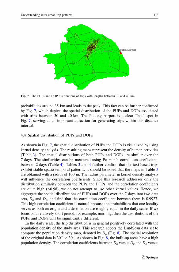
probabilities around 35 km and leads to the peak. This fact can be further confirmed

by Fig. 7, which depicts the spatial distribution of the PUPs and DOPs associated

with trips between 30 and 40 km. The Pudong Airport is a clear ‘‘hot’’ spot in

Fig. 7, serving as an important attraction for generating trips within this distance

interval.

4.4 Spatial distribution of PUPs and DOPs

As shown in Fig. 7, the spatial distribution of PUPs and DOPs is visualized by using

kernel density analysis. The resulting maps represent the density of human activities

(Table 3). The spatial distributions of both PUPs and DOPs are similar over the

7 days. The similarities can be measured using Pearson’s correlation coefficients

between 2 days (Table 4). Tables 3 and 4 further confirm that the taxi-based trips

exhibit stable spatio-temporal patterns. It should be noted that the maps in Table 3

are obtained with a radius of 100 m. The radius parameter in kernel density analysis

will influence the correlation coefficients. Since this research addresses only the

distribution similarity between the PUPs and DOPs, and the correlation coefficients

are quite high ([0.98), we do not attempt to use other kernel values. Hence, we

aggregate the spatial distributions of PUPs and DOPs over the 7 days into two data

sets, Du and Do, and find that the correlation coefficient between them is 0.9927.

This high correlation coefficient is natural because the probabilities that one locality

serves as both an origin and a destination are roughly equal in the daily scale. If we

focus on a relatively short period, for example, morning, then the distributions of the

PUPs and DOPs will be significantly different.

In the daily scale, the trip distribution is in general positively correlated with the

population density of the study area. This research adopts the LandScan data set to

compute the population density map, denoted by Dp (Fig. 8). The spatial resolution

of the original data is 3000 9 3000. As shown in Fig. 8, the built-up areas have a high

population density. The correlation coefficients between Du versus Dp and Do versus

Fig. 7 The PUPs and DOP distributions of trips with lengths between 30 and 40 km


123

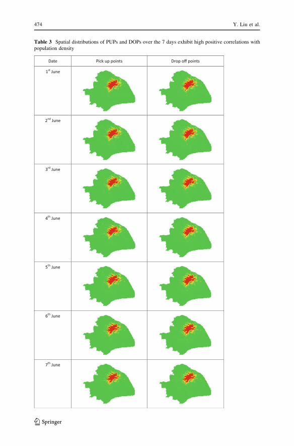
Table 3 Spatial distributions of PUPs and DOPs over the 7 days exhibit high positive correlations with

population density

474 Y. Liu et al.

123

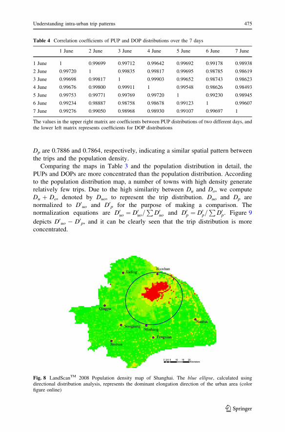
Dp are 0.7886 and 0.7864, respectively, indicating a similar spatial pattern between

the trips and the population density.

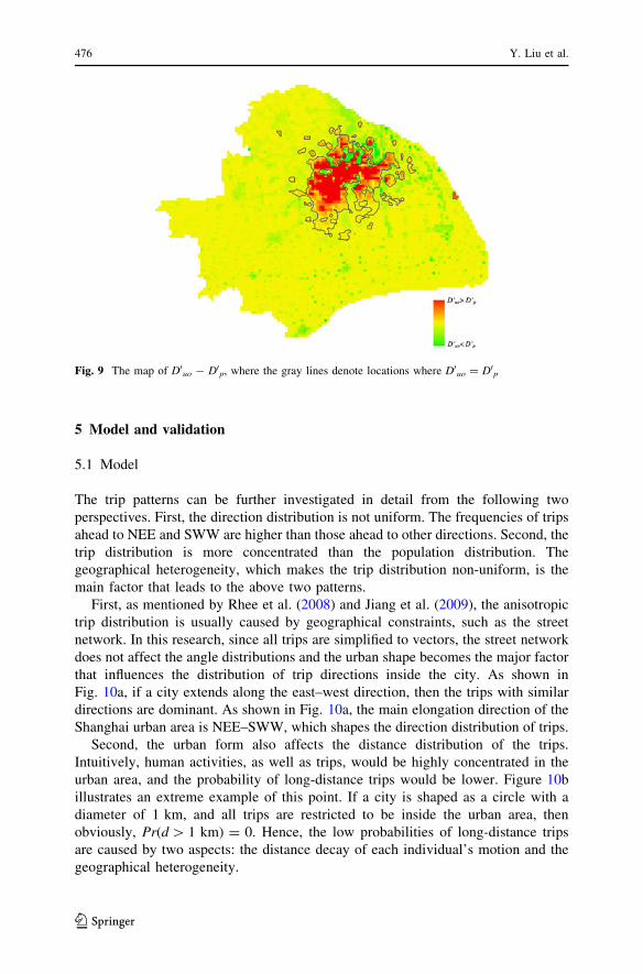
Comparing the maps in Table 3 and the population distribution in detail, the

PUPs and DOPs are more concentrated than the population distribution. According

to the population distribution map, a number of towns with high density generate

relatively few trips. Due to the high similarity between Du and Do, we compute

Du ? Do, denoted by Duo, to represent the trip distribution. Duo and Dp are

normalized to D0uo and D0p for the purpose of making a comparison. The

normalization equations are D0uo ¼ D0uo=P

D0uo and D0p ¼ D0p=P

D0p. Figure 9

depicts D0uo - D0p, and it can be clearly seen that the trip distribution is more

concentrated.

Fig. 8 LandScanTM 2008 Population density map of Shanghai. The blue ellipse, calculated usingdirectional distribution analysis, represents the dominant elongation direction of the urban area (colorfigure online)

Table 4 Correlation coefficients of PUP and DOP distributions over the 7 days

1 June 2 June 3 June 4 June 5 June 6 June 7 June

1 June 1 0.99699 0.99712 0.99642 0.99692 0.99178 0.98938

2 June 0.99720 1 0.99835 0.99817 0.99695 0.98785 0.98619

3 June 0.99698 0.99817 1 0.99903 0.99652 0.98743 0.98623

4 June 0.99676 0.99800 0.99911 1 0.99548 0.98626 0.98493

5 June 0.99753 0.99771 0.99769 0.99720 1 0.99230 0.98945

6 June 0.99234 0.98887 0.98758 0.98678 0.99123 1 0.99607

7 June 0.99276 0.99050 0.98968 0.98930 0.99107 0.99697 1

The values in the upper right matrix are coefficients between PUP distributions of two different days, and

the lower left matrix represents coefficients for DOP distributions


123

5 Model and validation

5.1 Model

The trip patterns can be further investigated in detail from the following two

perspectives. First, the direction distribution is not uniform. The frequencies of trips

ahead to NEE and SWW are higher than those ahead to other directions. Second, the

trip distribution is more concentrated than the population distribution. The

geographical heterogeneity, which makes the trip distribution non-uniform, is the

main factor that leads to the above two patterns.

First, as mentioned by Rhee et al. (2008) and Jiang et al. (2009), the anisotropic

trip distribution is usually caused by geographical constraints, such as the street

network. In this research, since all trips are simplified to vectors, the street network

does not affect the angle distributions and the urban shape becomes the major factor

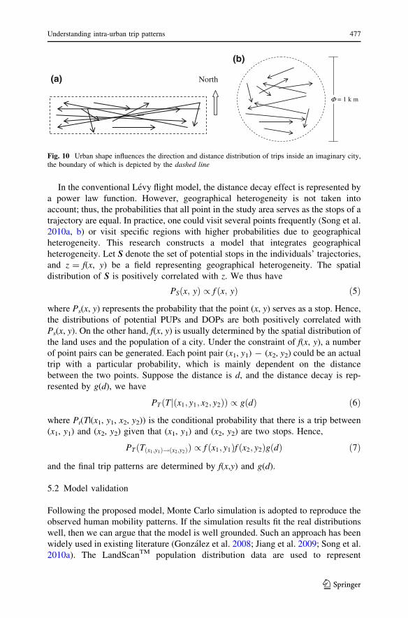
that influences the distribution of trip directions inside the city. As shown in

Fig. 10a, if a city extends along the east–west direction, then the trips with similar

directions are dominant. As shown in Fig. 10a, the main elongation direction of the

Shanghai urban area is NEE–SWW, which shapes the direction distribution of trips.

Second, the urban form also affects the distance distribution of the trips.

Intuitively, human activities, as well as trips, would be highly concentrated in the

urban area, and the probability of long-distance trips would be lower. Figure 10b

illustrates an extreme example of this point. If a city is shaped as a circle with a

diameter of 1 km, and all trips are restricted to be inside the urban area, then

obviously, Pr(d [ 1 km) = 0. Hence, the low probabilities of long-distance trips

are caused by two aspects: the distance decay of each individual’s motion and the

geographical heterogeneity.

Fig. 9 The map of D0uo - D0p, where the gray lines denote locations where D0uo = D0p

476 Y. Liu et al.

123

In the conventional Levy flight model, the distance decay effect is represented by

a power law function. However, geographical heterogeneity is not taken into

account; thus, the probabilities that all point in the study area serves as the stops of a

trajectory are equal. In practice, one could visit several points frequently (Song et al.

2010a, b) or visit specific regions with higher probabilities due to geographical

heterogeneity. This research constructs a model that integrates geographical

heterogeneity. Let S denote the set of potential stops in the individuals’ trajectories,

and z = f(x, y) be a field representing geographical heterogeneity. The spatial

distribution of S is positively correlated with z. We thus have

PSðx; yÞ / f ðx; yÞ ð5Þ

where Ps(x, y) represents the probability that the point (x, y) serves as a stop. Hence,

the distributions of potential PUPs and DOPs are both positively correlated with

Ps(x, y). On the other hand, f(x, y) is usually determined by the spatial distribution of

the land uses and the population of a city. Under the constraint of f(x, y), a number

of point pairs can be generated. Each point pair (x1, y1) - (x2, y2) could be an actual

trip with a particular probability, which is mainly dependent on the distance

between the two points. Suppose the distance is d, and the distance decay is rep-

resented by g(d), we have

PTðTjðx1; y1; x2; y2ÞÞ / gðdÞ ð6Þ

where Pt(T|(x1, y1, x2, y2)) is the conditional probability that there is a trip between

(x1, y1) and (x2, y2) given that (x1, y1) and (x2, y2) are two stops. Hence,

PTðTðx1;y1Þ!ðx2;y2ÞÞ / f ðx1; y1Þf ðx2; y2ÞgðdÞ ð7Þ

and the final trip patterns are determined by f(x,y) and g(d).

5.2 Model validation

Following the proposed model, Monte Carlo simulation is adopted to reproduce the

observed human mobility patterns. If the simulation results fit the real distributions

well, then we can argue that the model is well grounded. Such an approach has been

widely used in existing literature (Gonzalez et al. 2008; Jiang et al. 2009; Song et al.

2010a). The LandScanTM population distribution data are used to represent

North

Φ = 1 k m

(a)

(b)

Fig. 10 Urban shape influences the direction and distance distribution of trips inside an imaginary city,the boundary of which is depicted by the dashed line


123

geographical heterogeneity in this research. In other words, the densities of the

potential PUPs and DOPs are positively correlated with the population density.

Meanwhile, the power law distance decay is adopted, as follows:

gðdÞ ¼ ðd þ d0Þ�bd ð8Þ

where d0 is the cutoff distance and bd denotes the degree of distance decay in the

behavior associated with taking taxis. In the Monte Carlo simulations, generating a

synthetic trip includes three steps. First, a starting point is determined based on the

population density, using the method proposed in Liu et al. (2009). Second, the

candidate destination is generated following g(d) and a uniform direction distri-

bution. Finally, the acceptance-rejection method (Robert and Casella 2004) is

adopted to determine whether the obtained point pair should be accepted as an

actual trip according to the distribution of the population density. It should be noted

that the model does not take into account population heterogeneity, because all trips

are generated using the same g(d).

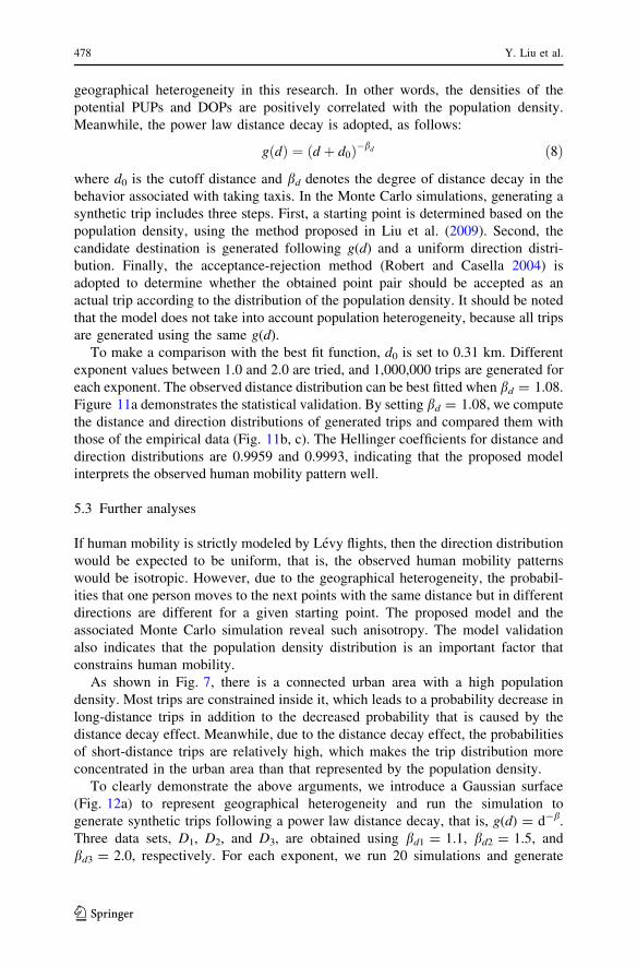
To make a comparison with the best fit function, d0 is set to 0.31 km. Different

exponent values between 1.0 and 2.0 are tried, and 1,000,000 trips are generated for

each exponent. The observed distance distribution can be best fitted when bd = 1.08.

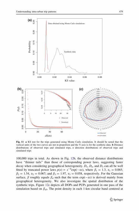
Figure 11a demonstrates the statistical validation. By setting bd = 1.08, we compute

the distance and direction distributions of generated trips and compared them with

those of the empirical data (Fig. 11b, c). The Hellinger coefficients for distance and

direction distributions are 0.9959 and 0.9993, indicating that the proposed model

interprets the observed human mobility pattern well.

5.3 Further analyses

If human mobility is strictly modeled by Levy flights, then the direction distribution

would be expected to be uniform, that is, the observed human mobility patterns

would be isotropic. However, due to the geographical heterogeneity, the probabil-

ities that one person moves to the next points with the same distance but in different

directions are different for a given starting point. The proposed model and the

associated Monte Carlo simulation reveal such anisotropy. The model validation

also indicates that the population density distribution is an important factor that

constrains human mobility.

As shown in Fig. 7, there is a connected urban area with a high population

density. Most trips are constrained inside it, which leads to a probability decrease in

long-distance trips in addition to the decreased probability that is caused by the

distance decay effect. Meanwhile, due to the distance decay effect, the probabilities

of short-distance trips are relatively high, which makes the trip distribution more

concentrated in the urban area than that represented by the population density.

To clearly demonstrate the above arguments, we introduce a Gaussian surface

(Fig. 12a) to represent geographical heterogeneity and run the simulation to

generate synthetic trips following a power law distance decay, that is, g(d) = d-b.

Three data sets, D1, D2, and D3, are obtained using bd1 = 1.1, bd2 = 1.5, and

bd3 = 2.0, respectively. For each exponent, we run 20 simulations and generate

478 Y. Liu et al.

123

100,000 trips in total. As shown in Fig. 12b, the observed distance distributions

have ‘‘thinner tails’’ than those of corresponding power laws, suggesting faster

decay when considering geographical heterogeneity. D1, D2, and D3 can all be well

fitted by truncated power laws p(x) � x-bexp(-ax), where b1 = 1.3, a1 = 0.065;

b2 = 1.54, a2 = 0.067; and b3 = 1.97, a3 = 0.058, respectively. For the Gaussian

surface, b roughly equals bd such that the term exp(-ax) is derived mainly from

geographical heterogeneity. We also investigate the spatial distribution of the

synthetic trips. Figure 12c depicts all DOPs and PUPs generated in one pass of the

simulation based on bd3. The point density in each 1-km circular band centered at

(a)

(b) (c)

0.00 0.02 0.04 0.06 0.08

0.00

0.05

0.10

0.15

0.20

0.25

KS value

Prob

abil

ity

Data obtained using Monte Carlo simulations

Synthetic data

0 20 40 60

0.00

0.05

0.10

0.15

0.20

0.25

d(km)

P(d

)

2 5 10 20 50

1e-0

51e

-03

1e-0

1

Observed

Simulated

Fig. 11 a KS test for the trips generated using Monte Carlo simulation. It should be noted that thevertical units of the two curves are not in proportion and the Y-axis is for the synthetic data. b Distancedistributions of observed trips and simulated trips, c direction distributions of observed trips andsimulated trips


123

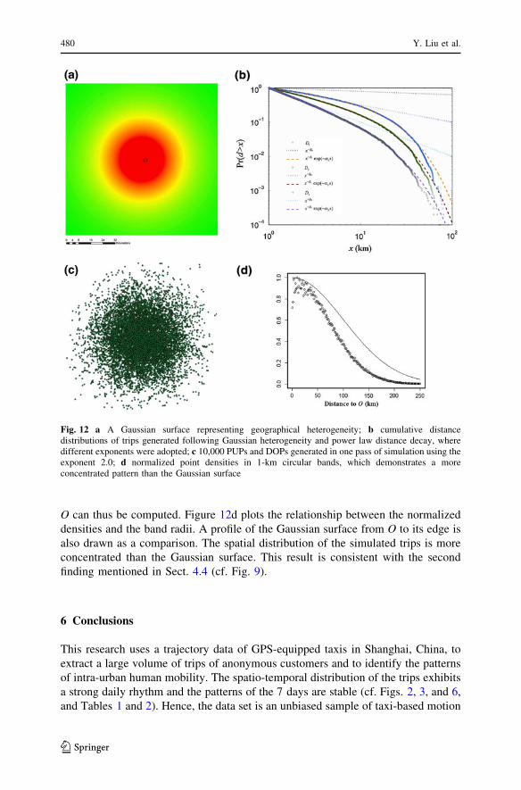
O can thus be computed. Figure 12d plots the relationship between the normalized

densities and the band radii. A profile of the Gaussian surface from O to its edge is

also drawn as a comparison. The spatial distribution of the simulated trips is more

concentrated than the Gaussian surface. This result is consistent with the second

finding mentioned in Sect. 4.4 (cf. Fig. 9).

6 Conclusions

This research uses a trajectory data of GPS-equipped taxis in Shanghai, China, to

extract a large volume of trips of anonymous customers and to identify the patterns

of intra-urban human mobility. The spatio-temporal distribution of the trips exhibits

a strong daily rhythm and the patterns of the 7 days are stable (cf. Figs. 2, 3, and 6,

and Tables 1 and 2). Hence, the data set is an unbiased sample of taxi-based motion

Fig. 12 a A Gaussian surface representing geographical heterogeneity; b cumulative distancedistributions of trips generated following Gaussian heterogeneity and power law distance decay, wheredifferent exponents were adopted; c 10,000 PUPs and DOPs generated in one pass of simulation using theexponent 2.0; d normalized point densities in 1-km circular bands, which demonstrates a moreconcentrated pattern than the Gaussian surface

480 Y. Liu et al.

123

of Shanghai citizens. Each trip is represented by a point pair and can be viewed as a

displacement in the random walk model.

We examine the distance and direction distributions of all extracted trips in this

study. The direction distribution is not uniform and has NEE–SWW as a major

direction, and the distance distribution can be fitted by an exponentially truncated

power law. To investigate the identified patterns, the LandScanTM population

density map is introduced to offer a global constraint to the spatial distribution of

the trips. Hence, given two points, the probability that there is a trip between them

depends on the population densities at the two points and the distance between

them, which represent geographical heterogeneity and distance decay, respectively.

These two aspects together influence the observed human mobility patterns. A

number of Monte Carlo simulations are run to generate synthetic trips, so that we

can compute the distance and direction distributions and compare them with

observed distributions. The comparison indicates that the proposed model interprets

well the observed patterns. This research achieves two findings. First, the major trip

direction is identical to the main elongation direction of the urban area. Second, the

distance distribution can be matched well when the power law distance decay

(d-1.08) is adopted. The exponent 1.08 indicates the inherent distance decay effect

of taxi-based trips. The observed decay d-1.2exp(-0.01d), however, has a ‘‘thinner

tail’’ than that of d-1.08, according to the trip distance distribution. These two

aspects can both be attributed to the geographical heterogeneity in the study area. In

most intra-urban human mobility studies, we can generally find one core urban area,

which shapes the direction distribution and enhances the distance decay observed in

the distance distribution. Nevertheless, the distance decay effect makes the spatial

distribution of the trips more concentrated. In summary, the geographical

heterogeneity and distance decay effect together influence the actual human

mobility patterns. Such an interaction is confirmed by a simulation based on

Gaussian geographical heterogeneity.

Compared with existing human mobility research based on the assumption that

the space is homogeneous, this research highlights the importance of geographical

heterogeneity in shaping the intra-urban human mobility. However, the population

heterogeneity is not considered in this research, since long-term individual

trajectories cannot be collected using the taxi data to measure the population

heterogeneity effect. Although the proposed model interprets the observed patterns

well, population heterogeneity should not be neglected. Shanghai has socio-spatial

differentiation on the subdistrict level in terms of attributes of employment sectors

such as the primary sector, secondary sector, and service sector, as well as migrant

status and educational attainment. The spatial distribution of residents working in

different employment sectors exhibits a concentric pattern, with the tertiary sector

concentrated in the downtown area (Li et al. 2007). Undoubtedly, employees in

different sections have different motion characteristics. These trends indicate that

population heterogeneity and geographical heterogeneity are tightly coupled. In the

future, we plan to use more detailed trajectory data to decouple the two types of

heterogeneity. To address the geographical heterogeneity, this research adopts

population density and finds that it is positively correlated with trip distributions.

However, some regions have low population density but relatively high trip


123

distributions. A good example is the Pudong Airport (cf. Fig. 7). It is reasonable that

many public facilities, such as railway stations, airports, and parks, attract more trips

than those estimated according to the population density. In future research, we plan

to introduce the distribution of POIs (point of interest) to investigate the spatial

characteristics of trips. A feasible approach is to estimate f(x, y), the field

influencing the probability that one point serves as a trajectory stop, using the

reverse gravity model (O’Kelly et al. 1995). The difference between f(x, y) and the

population distribution can be explained using the POI distributions.

Lastly, it should be noted that taxi data inevitably encounter issues of

representativeness, that is, mobile users and taxi passengers are not random

samples of the population. Another representativeness issue of the taxi data is that

one could choose different transportation modes, such as driving private vehicles,

taking a bus or subway, or taking a taxi for various trip purposes. It is natural that

different modes are associated with different patterns. For example, the exponents

representing the distance decay effect would be different. Hence, further investi-

gation is in need to generalize the patterns identified from taxi-based trips.

Acknowledgments This research is supported by NSFC (Grant nos. 40928001 and 41171296) and the

National High Technology Development 863 Program of China (Grant nos. 2011AA120301 and

2011AA120303).

References

Ahas R, Aasa A, Silm S, Tiru M (2010) Daily rhythms of suburban commuter’s movements in the Tallinn

metropolitan area: case study with mobile positioning data. Transport Res C Emer 18(1):45–54

Brockmann D, Theis F (2008) Money circulation, trackable items, and the emergence of universal human

mobility patterns. IEEE Pervas Comput 7(4):28–35

Brockmann D, Hufnagel L, Geisel T (2006) The scaling laws of human travel. Nature 439:463–465

Candia J, Gonzalez MC, Wang P, Schoenharl T, Madey G, Barabasi A-L (2008) Uncovering individual

and collective human dynamics from mobile phone records. J Phys A Math Theor

41(22):224015(1–11)

Cheng ZY, Caverlee J, Lee K, Sui DZ (2011) Exploring millions of footprints in location sharing services.

ICWSM 2011:81–88

Chowell G, Hyman JM, Eubank S, Castillo-Chavez C (2003) Scaling laws for the movement of people

between locations in a large city. Phys Rev E 68(6):066102(1–7)

Dai X, Ferman MA, Roesser RP (2003) A simulation evaluation of a real-time traffic information system

using probe vehicles. ITSC 1:475–480

Gonzalez MC, Hidalgo CA, Barabasi A-L (2008) Understanding individual human mobility patterns.

Nature 453:779–782

Hanson S, Huff J (1982) Assessing day to day variability in complex travel patterns. Transp Res Rec

891:18–24

Huff J, Hanson S (1986) Repetition and variability in urban travel. Geogr Anal 18(3):97–114

Jiang B, Yin J, Zhao S (2009) Characterizing the human mobility pattern in a large street network. Phys

Rev E 80(2):021136(1–11)

Kang H, Scott DM (2010) Exploring day-to-day variability in time use for household members. Transport

Res A Pol 44(8):609–619

Kuhne R, Schafer R-P, Mikat J, Thiessenhusen K-U, Bottger U, Lorkowski S (2003) New approaches for

traffic management in metropolitan areas. IFAC CTS 2003 symposium, Tokyo, Japan, 4–6 Aug

Lee K, Hong S, Kim SJ, Rhee I, Chong S (2009) SLAW: a mobility model for human walks. IEEE

INFOCOM 2009, pp 855–863

Li Z, Wu F, Gao X (2007) Global city polarization and socio-spatial restricting in Shanghai. Sci Geogr

Sinica 27(3):304–311

482 Y. Liu et al.

123

Li Q, Zhang T, Wang H, Zeng Z (2011) Dynamic accessibility mapping using floating car data: a

network-constrained density estimation approach. J Transp Geogr 19(3):379–393

Liu Y, Guo Q, Wieczorek J, Goodchild MF (2009) Positioning localities based on spatial assertions. Int J

Geogr Inf Sci 23(11):1471–1501

Liu L, Andris C, Ratti C (2010) Uncovering cabdrivers’ behaviour patterns from their digital traces.

Comput Environ Urban 34(6):541–548

Lu Y (2003) Getting away with the stolen vehicle: an investigation of journey-after-crime. Prof Geogr

55(4):422–433

Lu W, Zhu T, Wu D, Dai H, Huang J (2008) A heuristic path-estimating algorithm for large-scale real-

time traffic information calculating. Sci China Ser E 51(S1):165–174

O’Kelly ME, Song W, Shen G (1995) New estimates of gravitational attraction by linear programming.

Geogr Anal 27(4):271–285

Phithakkitnukoon S, Horanont T, Lorenzo GD, Shibasaki R, Ratti C (2010) Activity-aware map:

Identifying human daily activity pattern using mobile phone data. HBU 2010 LNCS 6219, pp 14–25

Qi G, Li X, Li S, Pan G, Wang Z, Zhang D (2011) Measuring social functions of city regions from large-

scale taxi behaviors. IEEE PERCOM Workshops, pp 384–388

Ratti C, Pulselli RM, Williams S, Frenchman D (2006) Mobile landscapes: using location data from cell

phones for urban analysis. Environ Plann B 33(5):727–748

Rhee I, Shin M, Hong S, Lee K, Chong S (2008) On the levy-walk nature of human mobility. IEEE

INFOCOM, pp 924–932

Robert CP, Casella G (2004) Monte Carlo statistical methods, 2nd edn. Springer, New York

Sang S, O’Kelly M, Kwan M-P (2011) Examining commuting patterns: results from a journey-to-work

model disaggregated by gender and occupation. Urban Stud 48(5):891–909

Schonfelder S, Axhausen KW (2010) Urban rhythms and travel behaviour: spatial and temporal

phenomena of daily travel. Ashgate Publishing, London

Sevtsuk A, Ratti C (2010) Does urban mobility have a daily routine? Learning from the aggregate data of

mobile networks. J Urban Technol 17(1):41–60

Shoval N (2008) Tracking technologies and urban analysis. Cities 25(1):21–28

Song C, Koren T, Wang P, Barabasi A-L (2010a) Modelling the scaling properties of human mobility.

Nat Phys 6(10):818–823

Song C, Qu Z, Blumm N, Barabasi A-L (2010b) Limits of predictability in human mobility. Science

327(5968):1018–1021

Sun J, Yuan J, Wang Y, Si H, Shan X (2011) Exploring space–time structure of human mobility in urban

space. Phys A 390(5):929–942

Susilo YO, Kitamura RK (2005) Analysis of the day-to-day variability in the individual’s action space: an

exploration of the six-week mobidrive travel diary data. Transp Res Rec 1902:124–133

Tong D, Coifman B, Merr CJ (2009) New perspectives on the use of GPS and GIS to support a highway

performance study. T GIS 13(1):69–85

Vegelius J, Janson S, Johansson F (1986) Measures of similarity between distributions. Qual Quant

20(4):437–441

Yuan Y, Raubal M, Liu Y (2012) Correlating mobile phone usage and travel behavior: a case study of

Harbin, China. Comput Environ Urban 36(2):118–130

Zheng Y, Liu Y, Yuan J, Xie X (2011) Urban computing with taxicabs. UbiComp 2011, pp 17–21


123

Documents

Understanding intra-urban trip patterns from taxi ...Received: 31 August 2011/Accepted: 5 March 2012/Published online: 21 March 2012 Springer-Verlag 2012 Abstract Intra-urban human