Embed Size (px)
Citation preview
Understanding Knee Points in Bicriteria Problems and Their
Implications as Preferred Solution Principles
Kalyanmoy Deb and Shivam GuptaKanpur Genetic Algorithms Laboratory (KanGAL)
Indian Institute of Technology KanpurPIN 208016, Uttar Pradesh, India
{deb,sgupta}@iitk.ac.in
KanGAL Report Number 2010005
July 5, 2010
Abstract
A knee point is almost always a preferred trade-off solution, if it exists in a bicriteria op-timization problem. In this paper, we make an attempt to better understand knee points andinvestigate the properties of bicriteria problems that may exhibit a knee on its Pareto-optimalfront. Specifically, we review past studies and suggest a couple of new definitions of a kneepoint. One of the definitions allows us to define a knee region for problems in which, instead ofone, a set of knee-like solutions exist. We also introduce edge-knee solutions which behave likea knee solution but lies near one of the extreme solutions. We argue here that knee solutionshave far-reaching implications than they are currently known for. It is an interesting fact thatin many problem-solving tasks, despite the existence of a number of solution methodologies,one or a few methodologies are commonly used. Here, we argue that often such common solu-tion principles are knee solutions to a bicriteria problem formed from two conflicting goals ofthe underlying problem-solving task. We illustrate our argument by show-casing a number ofpopularly used problem-solving tasks, such as regression, sorting, clustering and a number ofengineering design tasks. Each task, when viewed as a bicriteria problem, seems to exhibit aknee or a knee-region and the commonly used methodology seems to lie within the knee-region.Linking preferred solution methodologies as knee solutions to a related bicriteria problem iscertainly an interesting idea and may have a long-term implication in the development of ef-ficient solution methodologies for different scientific and other problem-solving tasks, such asgame-playing and strategic decision-making activities.
1 Introduction
Multi-objective optimization involves consideration of number of conflicting objectives. Theoreti-cally, such problems give rise to a set of optimal solutions, known as Pareto-optimal solutions, whichtogether constitute a trade-off front. In most cases, the front obtained by the Pareto-optimal solu-tions are such that the choice of a single preferred solution is not straightforward and a multi-criteriadecision-making methodology is needed to systematically choose a single preferred solution. How-ever, there exists certain multi-objective optimization problems which exhibit a knee point on theirPareto-optimal fronts. A knee point is almost always the most preferred solution, since it requiresan unfavorably large sacrifice in one objective to gain a small amount in the other objective. Kneepoints are well-recognized by multi-objective optimization researchers [3, 4, 5, 8, 13, 14, 15, 16, 18].Due to their natural preference compared to other Pareto-optimal solutions, some evolutionary
1
Engineering Optimization 2
optimization methodologies have been designed to find knee point(s) [3, 4, 8, 15, 16, 18]. However,a detailed study describing different plausible types of knee points and importantly addressing theissue on why some problems exhibit a knee solution is missing. In this paper, we review the existingdefinitions of a knee point and suggest a couple of new definitions for identifying a knee point in abicriteria optimization problem. The definitions allow us to describe other knee-like points whichhave not been categorized well in the multi-objective literature.
It is well argued that a knee point is a natural preferred solution, if exists in a multi-objectiveoptimization problem. In the subsequent part of this paper, we make an interesting and usefulconnection of a knee point with preferred solution methodologies often used in certain problem-solving tasks in practice. Scientists and engineers deal with different problem-solving tasks regularly,such as finding a mathematical regression equation fitting a set of two-dimensional data, clustering aset of two or three-dimensional data into a number of clusters, sorting a set of numbers in ascendingorder, finding root of an equation numerically, and others. In trying to solve such problems, thereis usually one or two methods which are commonly preferred in practice. We tried to find a linkbetween preferring specific methodologies in a problem-solving task with preferring knee pointsin a bicriteria optimization task. We argue that a plausible reason for why some methodologiesare preferred over other methods may come from this linking of a problem-solving task with anequivalent bi-objective problem and realizing that the preferred method may lie on the knee-regionof the corresponding trade-off front.
In the remainder of this paper, we review the existing definitions of a knee point. Thereafter,we suggest a couple of definitions based on a bend-angle based approach and another approach thatis dependent on an user’s preferred trade-off information. We describe systematic procedures foridentifying a knee point and illustrate their working principle on a tunable test problem exhibitinga knee point. In some problems, instead of a sole knee point, there may exist a set of closely-packed trade-off points that together qualify as a knee-region. Moreover, in certain problems, theknee point may exist near one of the extreme points of the trade-off front. We distinguish suchpoint(s) as edge-knee point(s). Based on gradient information, we then suggest some propertieswhich may cause a trade-off front to exhibit a knee point. This allows us to suggest a procedurefor designing bicriteria test problems having a knee point. In order to facilitate an user to estimatethe trade-off parameters in tune with the given trade-off frontier, we have also suggested a upperbound estimation procedure. In the remaining part of the paper, we consider a number of genericand engineering problems solving tasks and demonstrate that commonly-used solution principleslie near the knee-region of the associated bi-objective Pareto-optimal set. The concept of linkingpreferred solution principles as knee solutions of a derived bicriteria problem opens up interestingand far-reaching implications for developing efficient solution methodologies. Conclusions of thestudy are made thereafter.
2 A Knee Solution in a Bi-Objective Optimization Problem
Here, we restrict ourselves for minimization of two conflicting objectives only (fi : S → R, i = 1, 2)as functions of decision variables x:
minimize {f1(x), f2(x)} ,subject to x ∈ S,
(1)
where S ⊂ Rn denotes the set of feasible solutions. A vector consisting of objective function valuescalculated at some point x ∈ S is called an objective vector f(x) = (f1(x), f2(x))T .
2.1 Pareto-Optimal Points
Problem (1) gives rise to a set of Pareto-optimal solutions or a Pareto-optimal front (P ∗), providingtrade-off between two objectives. The domination between two solutions is defined as follows [7, 14]:

Engineering Optimization 3
C
f2
Α
Β
f1
Figure 1: The utility based definition of a kneepoint is illustrated.
angle f1
f2
Reflex
Figure 2: The reflex angle based definition ofa knee point is illustrated.
Definition 1 A solution x(1) is said to dominate the other solution x(2), if (i) the solution x(1) is noworse than x(2) in all objectives (that is, in the case of a minimization problem, fi(x
(1)) ≤ fi(x(2))
for all i = 1, 2) and (ii) the solution x(1) is strictly better than x(2) in at least one objective (thatis, in the case of a minimization problem, fi(x
(1)) < fi(x(2)) for at least one index i).
Pareto-optimal solutions are then defined as follows [14]:
Definition 2 A decision vector x∗ ∈ S is Pareto-optimal if there does not exist another decisionvector x ∈ S that dominates x∗ according to Definition 1.
2.2 Previous Definitions of a Knee Point
A previous study by Branke et. al.[4] for identifying a knee point used a couple of ideas. The firstdefinition was based on a linear marginal utility function: U(f , λ) = λf1 + (1− λ)f2 with λ ∈ [0,1]and f = (f1, f2)
T . The idea works as follows. First, a uniform set of weight values (λ) are chosenin [0, 1] and the best solution (having the minimum value of U) is identified for each λ. Followingdefinition is then used to define a knee point:
Definition 3 Let the minima-count of every Pareto-optimal solution is set to be zero initially. Forevery λi created uniformly in [0, 1], a Pareto-optimal solution j having the minimum U(f , λi) isidentified and its minima-count cj is incremented by one. After all λi ∈ [0, 1] are considered, thePareto-optimal solution having the maximum value of minima-count is defined as the knee point.
For a practical use of the above definition, a finite but a large set of λi values can be chosen.Figure 1 illustrates the scenario at which the knee1 point (marked as B) is minimum for a largernumber of utility functions than any other point on the Pareto-optimal front.
The second definition suggested in the study was based on finding two or more neighboringsolutions and calculating the reflex angle, as shown in Figure 2:
1The word ‘knee’ is appropriate for a scenario in which both objectives are to be maximized, as then the front
would look like a bended leg and the point of interest would lie on the knee part of the bended leg. In our opinion,
the word ‘elbow’ is more appropriate for minimization problems, but due to its wide-spread use, we shall continue to
refer to these solutions as ‘knee’ points, even for minimization problems.
Engineering Optimization 4
zn
(Knee point)
z
z*
Pz*
P
f1
f2A
B
Boundary line
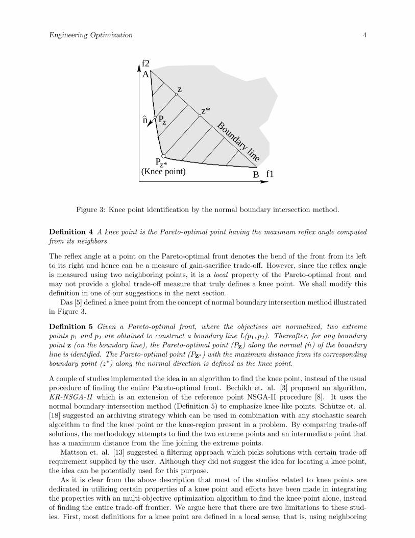
Figure 3: Knee point identification by the normal boundary intersection method.
Definition 4 A knee point is the Pareto-optimal point having the maximum reflex angle computedfrom its neighbors.
The reflex angle at a point on the Pareto-optimal front denotes the bend of the front from its leftto its right and hence can be a measure of gain-sacrifice trade-off. However, since the reflex angleis measured using two neighboring points, it is a local property of the Pareto-optimal front andmay not provide a global trade-off measure that truly defines a knee point. We shall modify thisdefinition in one of our suggestions in the next section.
Das [5] defined a knee point from the concept of normal boundary intersection method illustratedin Figure 3.
Definition 5 Given a Pareto-optimal front, where the objectives are normalized, two extremepoints p1 and p2 are obtained to construct a boundary line L(p1, p2). Thereafter, for any boundarypoint z (on the boundary line), the Pareto-optimal point (Pz) along the normal (n) of the boundaryline is identified. The Pareto-optimal point (Pz∗) with the maximum distance from its correspondingboundary point (z∗) along the normal direction is defined as the knee point.
A couple of studies implemented the idea in an algorithm to find the knee point, instead of the usualprocedure of finding the entire Pareto-optimal front. Bechikh et. al. [3] proposed an algorithm,KR-NSGA-II which is an extension of the reference point NSGA-II procedure [8]. It uses thenormal boundary intersection method (Definition 5) to emphasize knee-like points. Schutze et. al.[18] suggested an archiving strategy which can be used in combination with any stochastic searchalgorithm to find the knee point or the knee-region present in a problem. By comparing trade-offsolutions, the methodology attempts to find the two extreme points and an intermediate point thathas a maximum distance from the line joining the extreme points.
Mattson et. al. [13] suggested a filtering approach which picks solutions with certain trade-offrequirement supplied by the user. Although they did not suggest the idea for locating a knee point,the idea can be potentially used for this purpose.
As it is clear from the above description that most of the studies related to knee points arededicated in utilizing certain properties of a knee point and efforts have been made in integratingthe properties with an multi-objective optimization algorithm to find the knee point alone, insteadof finding the entire trade-off frontier. We argue here that there are two limitations to these stud-ies. First, most definitions for a knee point are defined in a local sense, that is, using neighboring
Engineering Optimization 5
points, except Das’s definition [5], which uses extreme point information. Second, all three def-initions mentioned above suffer from another difficulty. The Pareto-optimal solution having themaximum minima-count or having the maximum reflex angle or having the maximum deviationfrom the boundary line may still not correspond to a knee point providing certain desired trade-offinformation. Since no specific mention of trade-off was used in those definitions, they will alwaysrefer to a specific point as a knee point in every convex Pareto-optimal front. The correspondingminima-count, reflex angle or deviation measure may be marginally better than their neighborsand hence the adequacy of the corresponding point as a knee point is questionable. In the followingsection, we present two new definitions that require that a knee point must have a substantiallylarge trade-off value compared to other Pareto-optimal points, thereby having a global property.One of the definitions also utilizes user-supplied trade-off information directly. Later, we shallsuggest some interesting extensions to define other knee related points.
3 Proposed Knee Point Definitions
First, we present a definition that is similar in principle to the reflex angle approach discussedabove. Thereafter, we suggest a definition of a knee point that depends on user-supplied trade-offinformation directly.
3.1 Bend-Angle Approach
The computation of a reflex angle at a point x on the Pareto-optimal front requires two other points– a point (xL) left of x and another point (xR) right of x. Instead of computing the reflex anglefrom two neighbors of x, as suggested in the reflex angle approach [4], here, we define a bend-angle,that uses any two given Pareto-optimal points (xL,xR) left and right of x, respectively. For thecalculation of the bend-angle, we suggest here to use normalized values of the objectives, ratherthan the objectives themselves.
Definition 6 Let us say that for a given Pareto-optimal point x, two other Pareto-optimal pointsxL and xR, left and right of x are supplied. The bend-angle at x is defined as follows:
θ(x,xL,xR) = θL − θR, (2)
where
θL = arctanf2(x
L) − f2(x)
f1(x) − f1(xL), (3)
θR = arctanf2(x) − f2(x
R)
f1(xR) − f1(x). (4)
For any two supplied extreme trade-off points xL and xR, we now define a bend-angle based knee-point (xK
BA) as follows:
Definition 7 For a set of Pareto-optimal points, the point (x) having the maximum positive bend-angle θ(x,xL,xR) is identified. If the corresponding bend-angle is greater than a predefined thresholdSBA, the point x is a bend-angle based knee point.
It is clear from the above definition that there can be at most one knee point (xKBA) within the
range bounded by xL and xR. There is a fundamental difference between our definition and thereflex angle based definition [4]. Certain trade-off fronts may not have a knee point according to ourdefinition, but in reflex angle based definition there will always be at least one knee point for anytrade-off front. Moreover, our definition requires specification of two extreme points within which a
Engineering Optimization 6
Bend−angle
Point with maximumbend−angle
frontPareto−optimal
K
0.6
0.7
0.8
0.9
1
0 0.1 0.2 0.3 0.4 0.5 0.6 0.7 0.8 0.9 1
0.5
0.7
0.8
0.9
1
1.1
1.2
1.3
1.4
f2
Ben
d−A
ngle
(ra
d)
f1
0.4
0.3
0.2
0.1
0 0.6
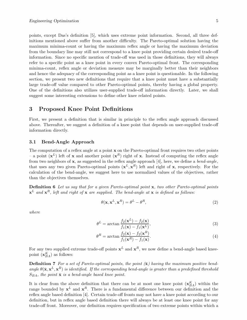
Figure 4: Pareto-optimal front for a = 0.1 and c = 0.1 and bend-angle values are shown.
knee point is sought. This definition has, therefore, a practical significance. Instead of seeking fora knee point on the entire Pareto-optimal front, the user can specify a region of interest and a kneepoint, if exists within the specified region would be identified. Furthermore, the specification of thethreshold SBA allows an user to achieve a desired sharpness of the obtained knee by calculating thedeviation of the (max) bend angle with the threshold SBA. Higher the deviation, more sharp andcrisp the point is, as a knee. Based on our estimation in a number of practical problems (discussedlater), we suggest SBA = 1 rad, which is equivalent to about 57.3 degrees.
We illustrate the above knee point definition to a hypothetical Pareto-optimal front describedmathematically as follows:
(af2 + f1 − a)(f2 + af1 − a) = ac2, (5)
where a and c are two parameters. The above function has two asymptotes: af2 + f1 − a = 0 andf2 + af1 − a = 0. The first asymptote has intercepts on f1 and f2 axes at a and 1, respectively,and the second asymptote has intercepts at 1 and a, respectively. The parameter a must be chosenless than one. The parameter c controls the degree of sharpness of the knee point. The smaller thevalue of c, more sharp is the knee point. Figure 4 shows the Pareto-optimal front for a = 0.1 andc = 0.1.
The corresponding bend-angle for every point on the front obtained using two extreme pointsf(xL) = (0, 1)T and f(xR) = (1, 0)T are shown in the figure. It is interesting to note how thebend-angle, starting with a small value close to left-extreme of the Pareto-optimal front, increasessharply and then falls quickly to small values near extreme right of the Pareto-optimal front. Sincethe knee point (xK
BA) corresponds to the point having the maximum bend-angle, the point K is acandidate point for a knee. Thereafter, we also observe from Figure 4 that the bend-angle at K isgreater than chosen threshold SBA = 1 rad. Thus, we declare the point K as the bend-angle basedknee point.
The trade-off frontier given in equation 5 can also be used to study the effect of sharpnessparameter (c) on the existence of a knee point. The above calculations were done for c = 0.1.Table 1 presents various knee point scenarios for different trade-off fronts obtained with different cvalues. As discussed above, as the value of c is increased the trade-off front becomes more and moreflat, thereby reducing the sharpness of the knee point. The maximum bend-angle obtained for eachc is also shown in the table. It is evident that with a threshold of 1 rad, all fronts below c ≤ 0.6
Engineering Optimization 7
Table 1: Effect of sharpness parameter c (with a = 0.1) on bend-angle based knee point.
cMaximum
f1 f2Bend-angle
0.0 1.370 0.0920 0.09080.1 1.303 0.1200 0.11930.2 1.239 0.1480 0.14880.3 1.179 0.1740 0.18040.4 1.123 0.2000 0.21200.5 1.072 0.2240 0.24590.6 1.026 0.2460 0.2821
0.7 0.982 0.2680 0.31840.8 0.943 0.2880 0.35730.9 0.906 0.3080 0.39631.0 0.871 0.3280 0.4355
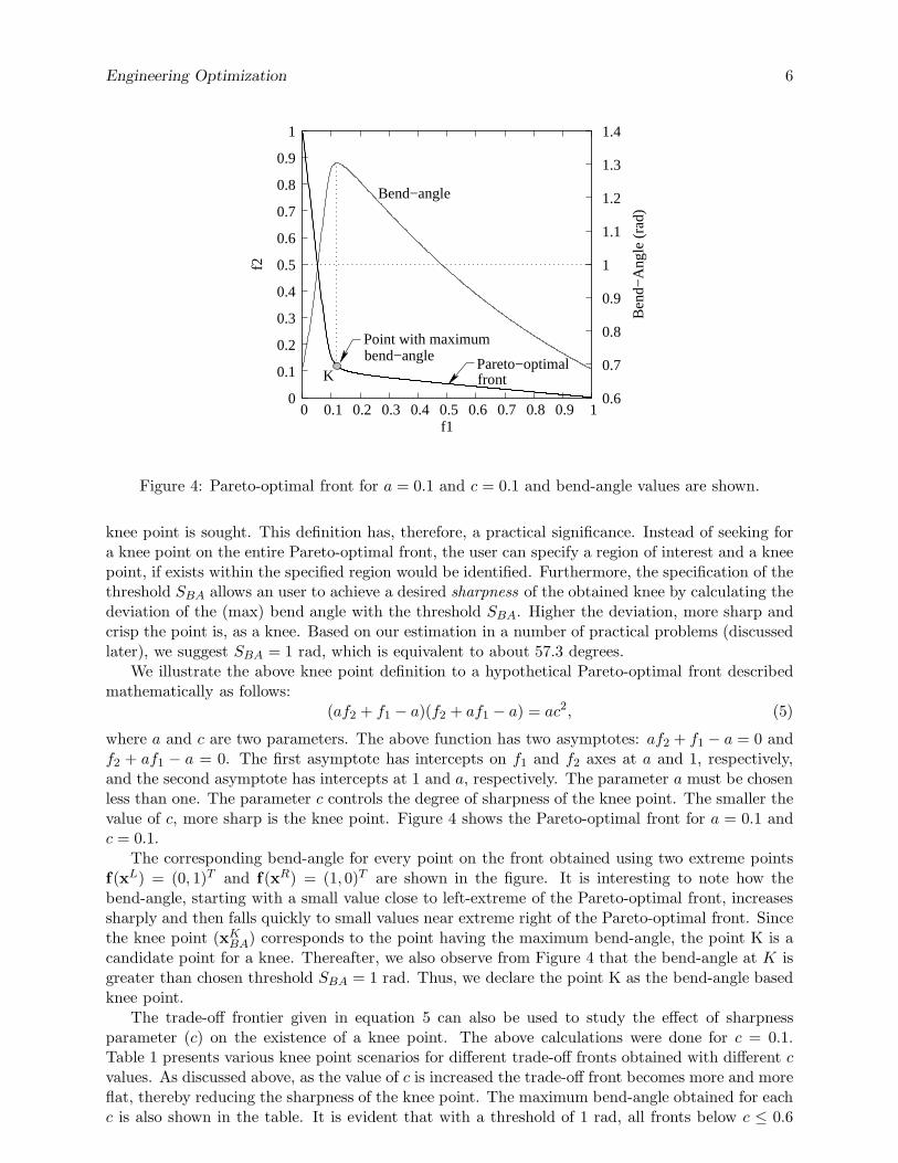
exhibit a bend-angle based knee, whereas for c ≥ 0.7, the corresponding fronts do not exhibit anyknee point. Figure 5 shows the trade-off fronts for four different c values: c = {0.0, 0.2, 0.4, 0.6}.The corresponding bend-angle based knee point is also marked on the respective front.
It is interesting to note that for a concave Pareto-optimal front, the bend-angle is negative forevery point. Since our definition requires the knee point to have a positive bend-angle, no kneepoint (xK
BA) exists for a purely concave Pareto-optimal front.
3.2 Trade-off Approach
Our next definition is directly related to the desired trade-off information that will define a kneepoint. Recall that a point is said to be a knee point if there does not exist any other point surpassinga desired trade-off. Let us say that we are interested in a knee point x with the following trade-off:A unit gain in f1 from x to any other trade-off point would require at least an amount of α sacrificein f2 and simultaneously a unit gain in f2 from x to any other point would require at least anamount of β sacrifice in f1. The parameters α and β are specified by the user. One advantageof this approach is that objectives need not be normalized; a proper choice (which can often bemotivated by their practical significance) of α and β can take care of different scaling of objectives.Since this method is directly related to the user-defined critical trade-off information, it is a morepragmatic approach.
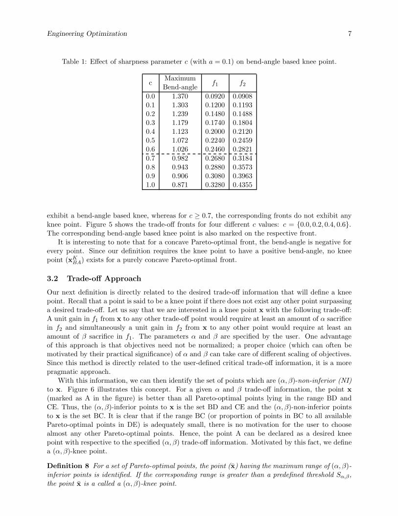
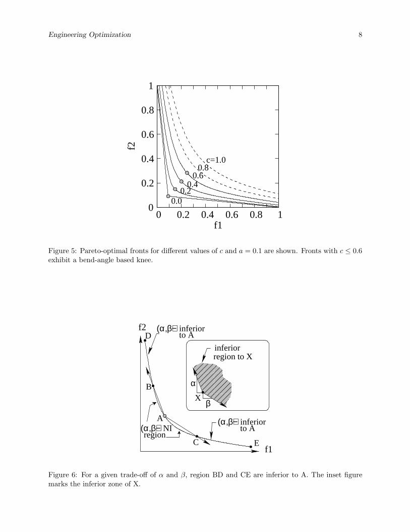
With this information, we can then identify the set of points which are (α, β)-non-inferior (NI)to x. Figure 6 illustrates this concept. For a given α and β trade-off information, the point x
(marked as A in the figure) is better than all Pareto-optimal points lying in the range BD andCE. Thus, the (α, β)-inferior points to x is the set BD and CE and the (α, β)-non-inferior pointsto x is the set BC. It is clear that if the range BC (or proportion of points in BC to all availablePareto-optimal points in DE) is adequately small, there is no motivation for the user to choosealmost any other Pareto-optimal points. Hence, the point A can be declared as a desired kneepoint with respective to the specified (α, β) trade-off information. Motivated by this fact, we definea (α, β)-knee point.
Definition 8 For a set of Pareto-optimal points, the point (x) having the maximum range of (α, β)-inferior points is identified. If the corresponding range is greater than a predefined threshold Sα,β,the point x is a called a (α, β)-knee point.
Engineering Optimization 8
0.00.2
0.4
c=1.0
0.60.8
0 0.2 0.4 0.6
0.4
0.8 1f1
f2
0.2
0
0.6
0.8
1
Figure 5: Pareto-optimal fronts for different values of c and a = 0.1 are shown. Fronts with c ≤ 0.6exhibit a bend-angle based knee.
��������������������
��������������������
inferior
to Ainferior
X
A
C E
D
α
β
inferiorregion to X
to A
B
f2
f1
(α,β)−
(α,β)−(α,β)−NIregion
Figure 6: For a given trade-off of α and β, region BD and CE are inferior to A. The inset figuremarks the inferior zone of X.

Engineering Optimization 9
Proportion of inferior
B
Inferior regions (BD and CE)
C
D
E
Threshold
inferior regionproportion of Point of max.
region
Pareto−optimal front
A
0.8 0.9 1 0
0.1
0.2
0.3
0.4
0.5
0.6
0.7
0.8
0.9
1
0.5
Pro
port
ion
of in
ferio
r re
gion
f1 0.4 0.3 0.2 0.1 0
1
0.8
0.6
0.4
0.2
0
f2
0.6 0.7
Figure 7: The (α, β)-knee point (A) for a = 0.1 and c = 0.3. The knee point maximizes theproportion of inferior region.
We illustrate this concept on the Pareto-optimal front given in equation 5. Figure 7 shows thefront with a = 0.1 and c = 0.3 and the corresponding knee point and region of (α, β)-inferior points(BD and CE) with α = β = 1.5. For different values of the sharpness factor c, the ratio of rangeof (α, β)-inferior points to the entire Pareto-optimal region is computed and tabulated in Table 2.It is clear from the second column that for c = 0, 100% points are (α, β)-inferior to the obtainedpoint, thereby clearly making the obtained point as a knee point. The knee point is also shown inthe table. As c is increased, the sharpness of the knee point reduces and the table indicates thatthe maximum proportion of (α, β)-inferior region to the entire front region decreases. To make anagreement with the bend-angle approach, we suggest and set Sα,β = 0.82 here, so that all frontswith c ≤ 0.6 qualify to have a (α, β)-knee point.
For concave Pareto-optimal fronts, extreme points (or their neighbors) are likely candidate of a(α, β)-knee point and it is impossible that an intermediate point will qualify as a (α, β)-knee pointby the above definition.
Both bend angle and (α, β) approach tries to capture the trade-off information from the Pareto-optimal front and use a metric to quantify this trade-off information. If this metric for a particularpoint is greater than a chosen threshold, the point qualifies as a knee point, otherwise there is noknee point. This essential concept was missing in previous approaches, such as the reflex angle,utility and normal boundary intersection approaches. However, since each of these methods alsoutilize a metric namely, reflex angle, utility and distance in its core, the definitions can be modifiedby restricting their values to essentially lie beyond a certain threshold before a point can be declaredas a knee point.
4 Knee-Region
The above two definitions allow us to determine the existence of a knee point (parameterizedwith respect to user specifications) and locate it from a given bi-objective Pareto-optimal front.However, if we focus on some fronts, such as the one with c = 0.3 in Figure 7, we find that thereare other knee-like points around the obtained knee point. Although the point A is declared as
Engineering Optimization 10
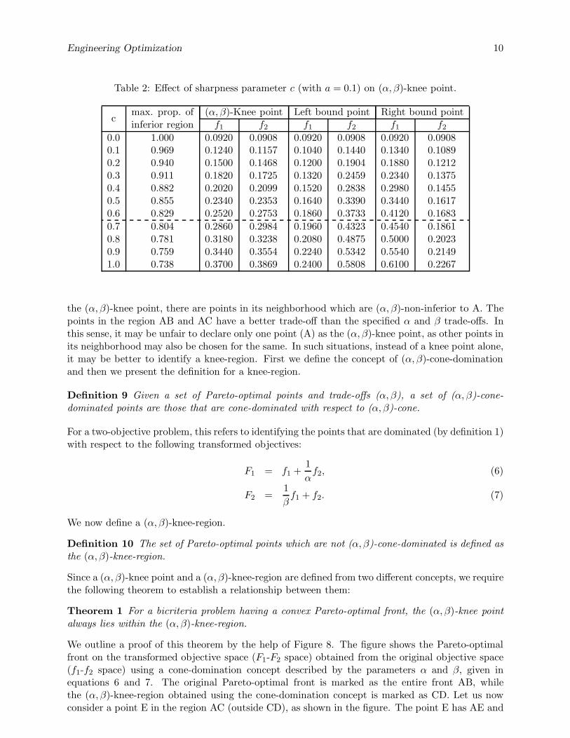
Table 2: Effect of sharpness parameter c (with a = 0.1) on (α, β)-knee point.
cmax. prop. of (α, β)-Knee point Left bound point Right bound pointinferior region f1 f2 f1 f2 f1 f2
0.0 1.000 0.0920 0.0908 0.0920 0.0908 0.0920 0.09080.1 0.969 0.1240 0.1157 0.1040 0.1440 0.1340 0.10890.2 0.940 0.1500 0.1468 0.1200 0.1904 0.1880 0.12120.3 0.911 0.1820 0.1725 0.1320 0.2459 0.2340 0.13750.4 0.882 0.2020 0.2099 0.1520 0.2838 0.2980 0.14550.5 0.855 0.2340 0.2353 0.1640 0.3390 0.3440 0.16170.6 0.829 0.2520 0.2753 0.1860 0.3733 0.4120 0.1683
0.7 0.804 0.2860 0.2984 0.1960 0.4323 0.4540 0.18610.8 0.781 0.3180 0.3238 0.2080 0.4875 0.5000 0.20230.9 0.759 0.3440 0.3554 0.2240 0.5342 0.5540 0.21491.0 0.738 0.3700 0.3869 0.2400 0.5808 0.6100 0.2267
the (α, β)-knee point, there are points in its neighborhood which are (α, β)-non-inferior to A. Thepoints in the region AB and AC have a better trade-off than the specified α and β trade-offs. Inthis sense, it may be unfair to declare only one point (A) as the (α, β)-knee point, as other points inits neighborhood may also be chosen for the same. In such situations, instead of a knee point alone,it may be better to identify a knee-region. First we define the concept of (α, β)-cone-dominationand then we present the definition for a knee-region.
Definition 9 Given a set of Pareto-optimal points and trade-offs (α, β), a set of (α, β)-cone-dominated points are those that are cone-dominated with respect to (α, β)-cone.
For a two-objective problem, this refers to identifying the points that are dominated (by definition 1)with respect to the following transformed objectives:
F1 = f1 +1
αf2, (6)
F2 =1
βf1 + f2. (7)
We now define a (α, β)-knee-region.
Definition 10 The set of Pareto-optimal points which are not (α, β)-cone-dominated is defined asthe (α, β)-knee-region.
Since a (α, β)-knee point and a (α, β)-knee-region are defined from two different concepts, we requirethe following theorem to establish a relationship between them:
Theorem 1 For a bicriteria problem having a convex Pareto-optimal front, the (α, β)-knee pointalways lies within the (α, β)-knee-region.
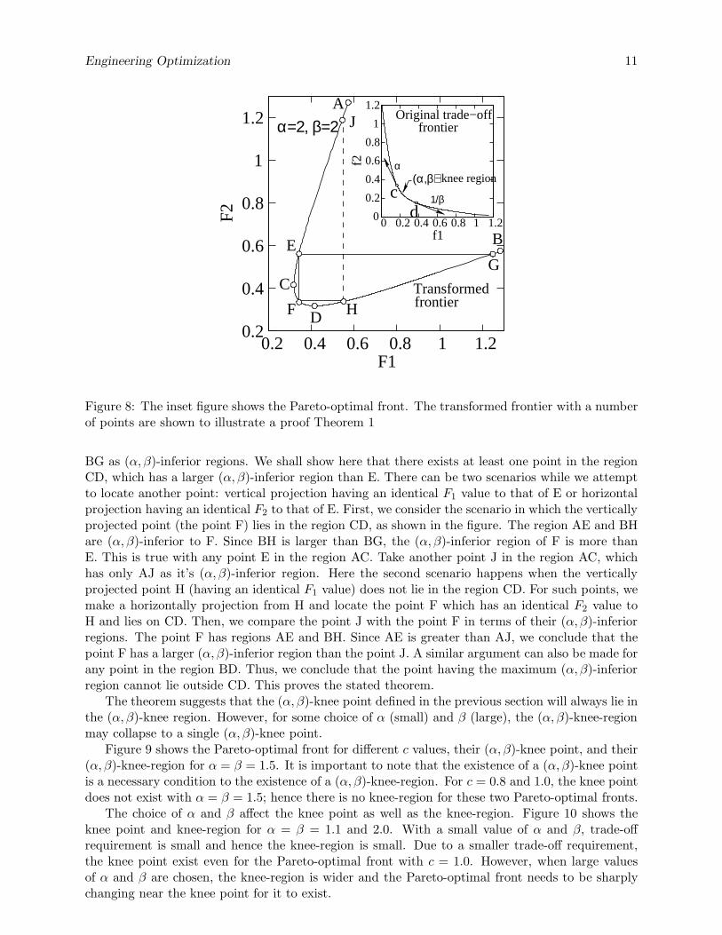
We outline a proof of this theorem by the help of Figure 8. The figure shows the Pareto-optimalfront on the transformed objective space (F1-F2 space) obtained from the original objective space(f1-f2 space) using a cone-domination concept described by the parameters α and β, given inequations 6 and 7. The original Pareto-optimal front is marked as the entire front AB, whilethe (α, β)-knee-region obtained using the cone-domination concept is marked as CD. Let us nowconsider a point E in the region AC (outside CD), as shown in the figure. The point E has AE and
Engineering Optimization 11
D
Transformed
A
α=2, β=2 frontierOriginal trade−off
α
1/β
−knee region(α,β)
J
G
B
HF
E
Cfrontier
0.4
0.2
F2
0
0.2
0.4
0.6
0.8
1
1.2
0 0.2
0.4
0.6 0.8 1 1.2f1
f2
0.4
0.6 0.8 1 1.2F1
0.2
1.2
1
0.8
0.6
cd
Figure 8: The inset figure shows the Pareto-optimal front. The transformed frontier with a numberof points are shown to illustrate a proof Theorem 1
BG as (α, β)-inferior regions. We shall show here that there exists at least one point in the regionCD, which has a larger (α, β)-inferior region than E. There can be two scenarios while we attemptto locate another point: vertical projection having an identical F1 value to that of E or horizontalprojection having an identical F2 to that of E. First, we consider the scenario in which the verticallyprojected point (the point F) lies in the region CD, as shown in the figure. The region AE and BHare (α, β)-inferior to F. Since BH is larger than BG, the (α, β)-inferior region of F is more thanE. This is true with any point E in the region AC. Take another point J in the region AC, whichhas only AJ as it’s (α, β)-inferior region. Here the second scenario happens when the verticallyprojected point H (having an identical F1 value) does not lie in the region CD. For such points, wemake a horizontally projection from H and locate the point F which has an identical F2 value toH and lies on CD. Then, we compare the point J with the point F in terms of their (α, β)-inferiorregions. The point F has regions AE and BH. Since AE is greater than AJ, we conclude that thepoint F has a larger (α, β)-inferior region than the point J. A similar argument can also be made forany point in the region BD. Thus, we conclude that the point having the maximum (α, β)-inferiorregion cannot lie outside CD. This proves the stated theorem.
The theorem suggests that the (α, β)-knee point defined in the previous section will always lie inthe (α, β)-knee region. However, for some choice of α (small) and β (large), the (α, β)-knee-regionmay collapse to a single (α, β)-knee point.
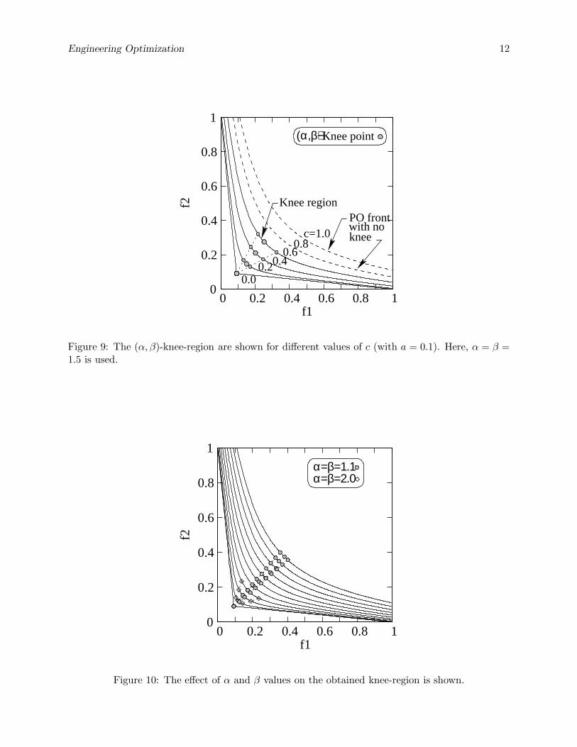
Figure 9 shows the Pareto-optimal front for different c values, their (α, β)-knee point, and their(α, β)-knee-region for α = β = 1.5. It is important to note that the existence of a (α, β)-knee pointis a necessary condition to the existence of a (α, β)-knee-region. For c = 0.8 and 1.0, the knee pointdoes not exist with α = β = 1.5; hence there is no knee-region for these two Pareto-optimal fronts.
The choice of α and β affect the knee point as well as the knee-region. Figure 10 shows theknee point and knee-region for α = β = 1.1 and 2.0. With a small value of α and β, trade-offrequirement is small and hence the knee-region is small. Due to a smaller trade-off requirement,the knee point exist even for the Pareto-optimal front with c = 1.0. However, when large valuesof α and β are chosen, the knee-region is wider and the Pareto-optimal front needs to be sharplychanging near the knee point for it to exist.
Engineering Optimization 12
(α,β)−
c=1.00.8
0.6
PO frontwith noknee
Knee region
0.00.20.4
Knee point
0 0.6 0.8 1
f2
f1 0.2 0
1
0.8
0.6
0.4
0.2
0.4
Figure 9: The (α, β)-knee-region are shown for different values of c (with a = 0.1). Here, α = β =1.5 is used.
α=β=2.0α=β=1.1
f2
0.6
0.8
1
0 0.2 0.4 0.6 0.8 1f1
0.2
0
0.4
Figure 10: The effect of α and β values on the obtained knee-region is shown.
Engineering Optimization 13
Edge−knee regionf2
gainsacrifice
f2
f1
gain
sacr
ifice
kneeEdge−
f1
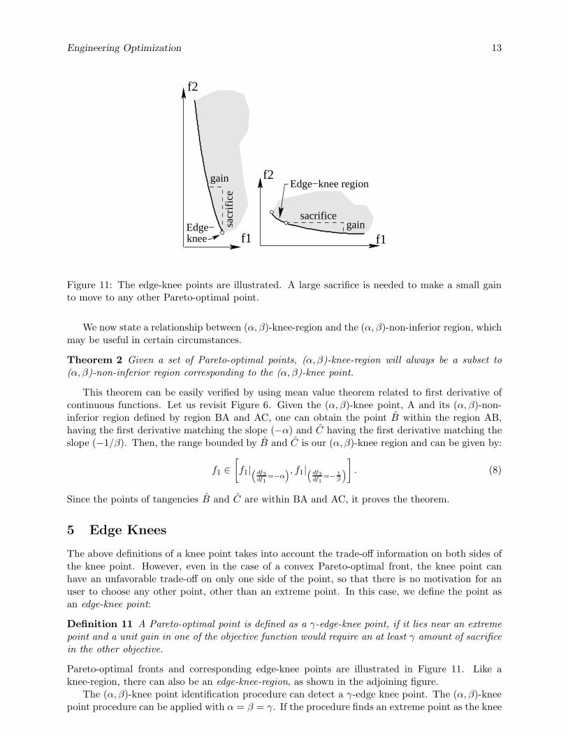
Figure 11: The edge-knee points are illustrated. A large sacrifice is needed to make a small gainto move to any other Pareto-optimal point.
We now state a relationship between (α, β)-knee-region and the (α, β)-non-inferior region, whichmay be useful in certain circumstances.
Theorem 2 Given a set of Pareto-optimal points, (α, β)-knee-region will always be a subset to(α, β)-non-inferior region corresponding to the (α, β)-knee point.
This theorem can be easily verified by using mean value theorem related to first derivative ofcontinuous functions. Let us revisit Figure 6. Given the (α, β)-knee point, A and its (α, β)-non-inferior region defined by region BA and AC, one can obtain the point B within the region AB,having the first derivative matching the slope (−α) and C having the first derivative matching theslope (−1/β). Then, the range bounded by B and C is our (α, β)-knee region and can be given by:
f1 ∈
[
f1|“ df2df1
=−α”, f1|“ df2
df1=−
1
β
”
]
. (8)
Since the points of tangencies B and C are within BA and AC, it proves the theorem.
5 Edge Knees
The above definitions of a knee point takes into account the trade-off information on both sides ofthe knee point. However, even in the case of a convex Pareto-optimal front, the knee point canhave an unfavorable trade-off on only one side of the point, so that there is no motivation for anuser to choose any other point, other than an extreme point. In this case, we define the point asan edge-knee point:
Definition 11 A Pareto-optimal point is defined as a γ-edge-knee point, if it lies near an extremepoint and a unit gain in one of the objective function would require an at least γ amount of sacrificein the other objective.
Pareto-optimal fronts and corresponding edge-knee points are illustrated in Figure 11. Like aknee-region, there can also be an edge-knee-region, as shown in the adjoining figure.
The (α, β)-knee point identification procedure can detect a γ-edge knee point. The (α, β)-kneepoint procedure can be applied with α = β = γ. If the procedure finds an extreme point as the knee
Engineering Optimization 14
Prop. of inferior
Domina
ted
front
BC
A Edge−knee point
frontPareto−optimal
region
0.6 0.8 1 0
0.2
0.4
0.6
0.8
1
0
f2
1
0.8
0.6
0.4
Pro
p. o
f inf
erio
r re
gion
0.2
0
f1 0.2 0.4
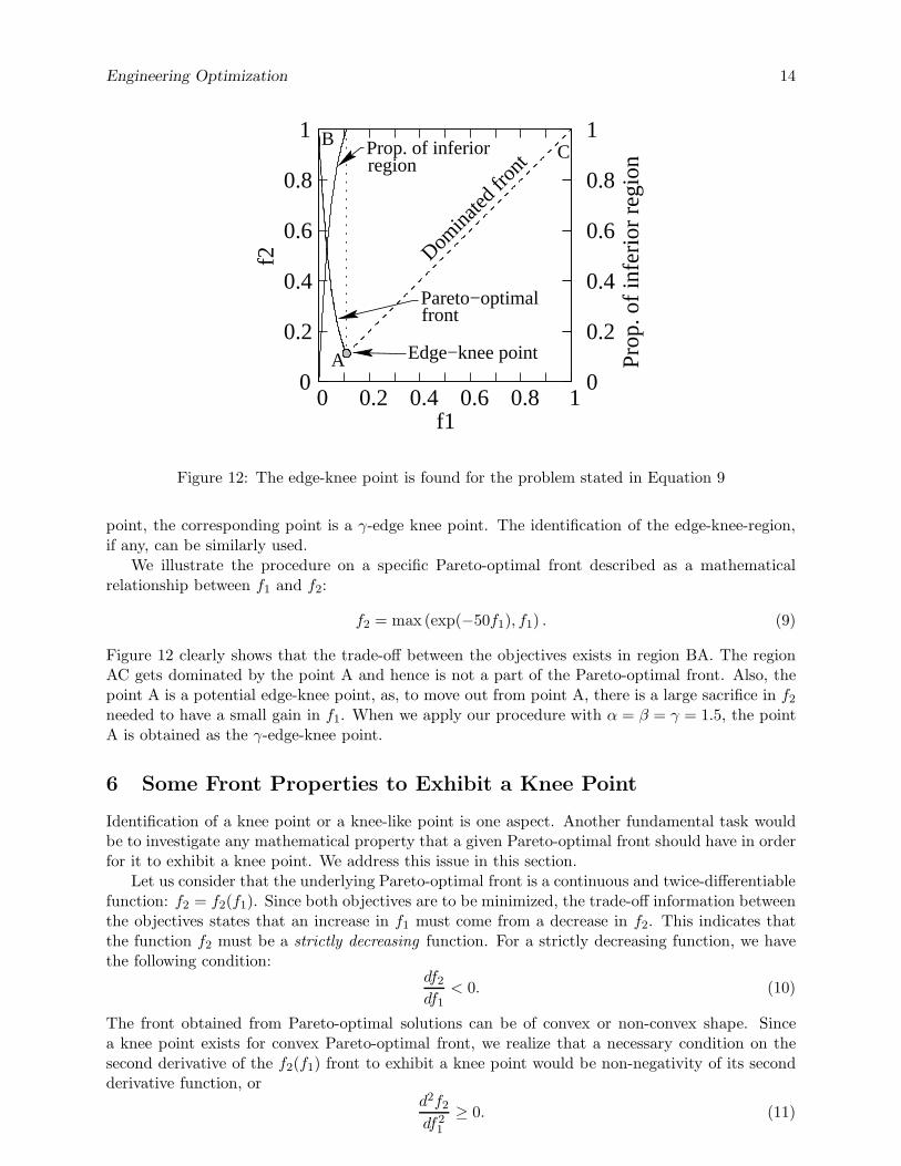
Figure 12: The edge-knee point is found for the problem stated in Equation 9
point, the corresponding point is a γ-edge knee point. The identification of the edge-knee-region,if any, can be similarly used.
We illustrate the procedure on a specific Pareto-optimal front described as a mathematicalrelationship between f1 and f2:
f2 = max (exp(−50f1), f1) . (9)
Figure 12 clearly shows that the trade-off between the objectives exists in region BA. The regionAC gets dominated by the point A and hence is not a part of the Pareto-optimal front. Also, thepoint A is a potential edge-knee point, as, to move out from point A, there is a large sacrifice in f2
needed to have a small gain in f1. When we apply our procedure with α = β = γ = 1.5, the pointA is obtained as the γ-edge-knee point.
6 Some Front Properties to Exhibit a Knee Point
Identification of a knee point or a knee-like point is one aspect. Another fundamental task wouldbe to investigate any mathematical property that a given Pareto-optimal front should have in orderfor it to exhibit a knee point. We address this issue in this section.
Let us consider that the underlying Pareto-optimal front is a continuous and twice-differentiablefunction: f2 = f2(f1). Since both objectives are to be minimized, the trade-off information betweenthe objectives states that an increase in f1 must come from a decrease in f2. This indicates thatthe function f2 must be a strictly decreasing function. For a strictly decreasing function, we havethe following condition:
df2
df1< 0. (10)
The front obtained from Pareto-optimal solutions can be of convex or non-convex shape. Sincea knee point exists for convex Pareto-optimal front, we realize that a necessary condition on thesecond derivative of the f2(f1) front to exhibit a knee point would be non-negativity of its secondderivative function, or
d2f2
df21
≥ 0. (11)
Engineering Optimization 15
First deriv.
frontPareto−optimal
f2
0.8
1
0 0.2 0.4 0.6 0.8 1−10
−8
−6
−4
−2
0
Firs
t Der
ivat
ive
of f2
wrt
f1
f1
0.4
0.2
0
0.6
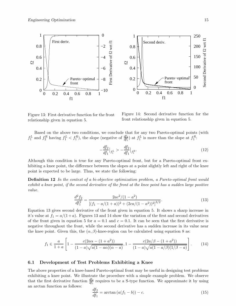
Figure 13: First derivative function for the frontrelationship given in equation 5.
Second deriv.
frontPareto−optimal
f2
0.8
1
0 0.2 0.4 0.6 0.8 1 0
50
100
150
200
250
Sec
ond
Der
ivat
ive
of f2
wrt
f1
f1
0.4
0.2
0
0.6
Figure 14: Second derivative function for thefront relationship given in equation 5.
Based on the above two conditions, we conclude that for any two Pareto-optimal points (withfL1 and fR
2 having fL1 < fR
1 ), the slope (negative of df2
df1) at fL
1 is more than the slope at fR1 :
−df2
df1
∣
∣
fL1
> −df2
df1
∣
∣
fR1
. (12)
Although this condition is true for any Pareto-optimal front, but for a Pareto-optimal front ex-hibiting a knee point, the difference between the slopes at a point slightly left and right of the kneepoint is expected to be large. Thus, we state the following:
Definition 12 In the context of a bi-objective optimization problem, a Pareto-optimal front wouldexhibit a knee point, if the second derivative of the front at the knee point has a sudden large positivevalue.
d2f2
df21
=2ac2/(1 − a2)
[(f1 − a/(1 + a))2 + (2ca/(1 − a2))2]3/2. (13)
Equation 13 gives second derivative of the front given in equation 5. It shows a sharp increase init’s value at f1 = a/(1+a). Figures 13 and 14 show the variation of the first and second derivativesof the front given in equation 5 for a = 0.1 and c = 0.1. It can be seen that the first derivative isnegative throughout the front, while the second derivative has a sudden increase in its value nearthe knee point. Given this, the (α, β)-knee-region can be calculated using equation 8 as:
f1 ∈a
1 + a
[
1 −c(2aα − (1 + a2))
(1 − a)√
a(1 − aα)(α − a), 1 −
c(2a/β − (1 + a2))
(1 − a)√
a(1 − a/β)(1/β − a)
]
. (14)
6.1 Development of Test Problems Exhibiting a Knee
The above properties of a knee-based Pareto-optimal front may be useful in designing test problemsexhibiting a knee point. We illustrate the procedure with a simple example problem. We observethat the first derivative function df2
df1requires to be a S-type function. We approximate it by using
an arctan function as follows:df2
df1= arctan (a(f1 − b)) − c. (15)
Engineering Optimization 16
}(2,2)−knee region
(2,2)−knee point
Pareto−optimal front
First derivative
0
0.5
1
1.5
0 2 4 6 8 10−3.5
−1.5−2.5
−2
−1.5
−1
−0.5
0f2
Firs
t Der
ivat
ive
of f2
wrt
f1
f1
−2
−2.5
−3
−1
−0.5
(arctan function)
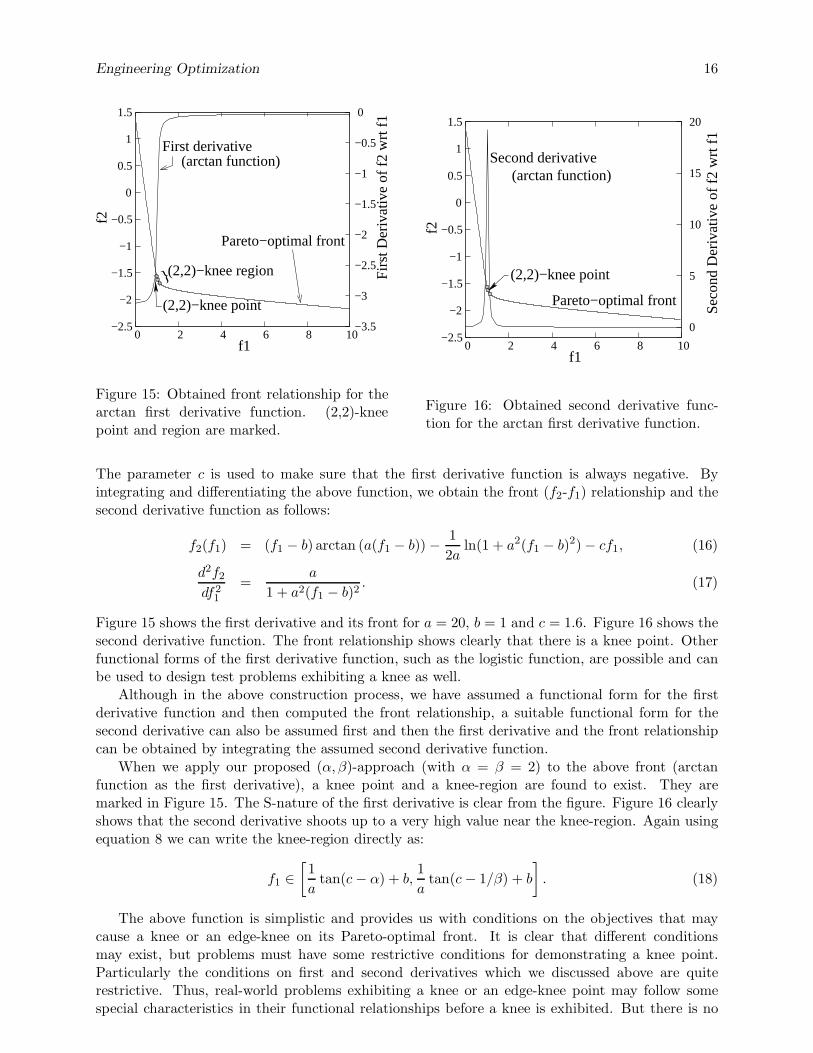
Figure 15: Obtained front relationship for thearctan first derivative function. (2,2)-kneepoint and region are marked.
Pareto−optimal front
Second derivative
(2,2)−knee point−1
−0.5
0
0.5
1
1.5
0 2 4 6−2.5
10
0
5
10
15
20
f2
Sec
ond
Der
ivat
ive
of f2
wrt
f1
f1 8
−2
−1.5
(arctan function)
Figure 16: Obtained second derivative func-tion for the arctan first derivative function.
The parameter c is used to make sure that the first derivative function is always negative. Byintegrating and differentiating the above function, we obtain the front (f2-f1) relationship and thesecond derivative function as follows:
f2(f1) = (f1 − b) arctan (a(f1 − b)) −1
2aln(1 + a2(f1 − b)2) − cf1, (16)
d2f2
df21
=a
1 + a2(f1 − b)2. (17)
Figure 15 shows the first derivative and its front for a = 20, b = 1 and c = 1.6. Figure 16 shows thesecond derivative function. The front relationship shows clearly that there is a knee point. Otherfunctional forms of the first derivative function, such as the logistic function, are possible and canbe used to design test problems exhibiting a knee as well.
Although in the above construction process, we have assumed a functional form for the firstderivative function and then computed the front relationship, a suitable functional form for thesecond derivative can also be assumed first and then the first derivative and the front relationshipcan be obtained by integrating the assumed second derivative function.
When we apply our proposed (α, β)-approach (with α = β = 2) to the above front (arctanfunction as the first derivative), a knee point and a knee-region are found to exist. They aremarked in Figure 15. The S-nature of the first derivative is clear from the figure. Figure 16 clearlyshows that the second derivative shoots up to a very high value near the knee-region. Again usingequation 8 we can write the knee-region directly as:
f1 ∈
[
1
atan(c − α) + b,
1
atan(c − 1/β) + b
]
. (18)
The above function is simplistic and provides us with conditions on the objectives that maycause a knee or an edge-knee on its Pareto-optimal front. It is clear that different conditionsmay exist, but problems must have some restrictive conditions for demonstrating a knee point.Particularly the conditions on first and second derivatives which we discussed above are quiterestrictive. Thus, real-world problems exhibiting a knee or an edge-knee point may follow somespecial characteristics in their functional relationships before a knee is exhibited. But there is no
Engineering Optimization 17
denying that if there exists a knee to a two-objective optimization problem, the knee point is themost preferred. We shall argue a connection between the above property of a knee point withpopular solution methodologies used in certain problem-solving tasks, but before that we suggesta procedure which may help provide some a priori information about adequate values of trade-offparameters (α and β) in a trade-off frontier exhibiting a knee point.
7 Upper Bound Estimation for Trade-off Parameters
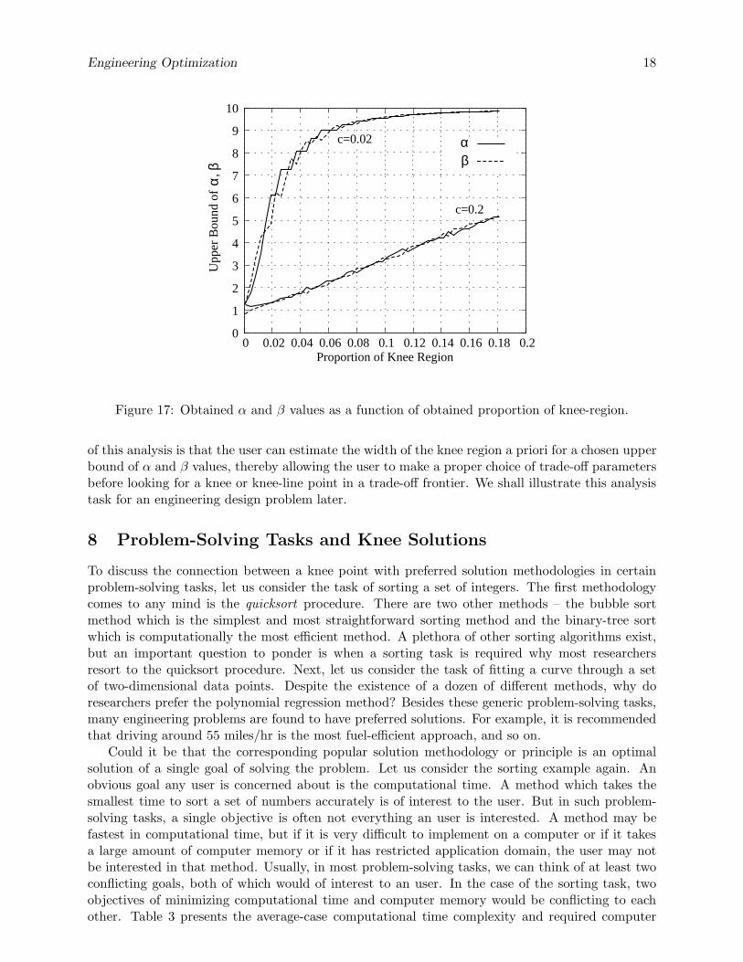
In the trade-off approach mentioned above, it is expected that the user will supply two trade-off parameters: left-side trade-off, α and right-side trade-off, β. This allows the user to provideproblem-specific information in determining a knee point or a knee-region. But, given a trade-offfrontier, we can also analyze and find the upper bounds on these parameters which will cause thefrontier to exhibit a knee like property.
Recall that in addition to a knee point, a trade-off frontier is expected to have a knee-region ofcertain width, depending on the chosen α and β parameters. Since these two parameters will besupplied by the user before a knee-point or a knee-region is found, the user may be interested inknowing the upper limit of these two parameters for a particular width of the resulting knee-region.If the chosen width is small, it is expected that a sharp knee point is desired, and vice versa. Todetermine such limits, we suggest an inverse analysis process to that portrayed in the previoussection here.
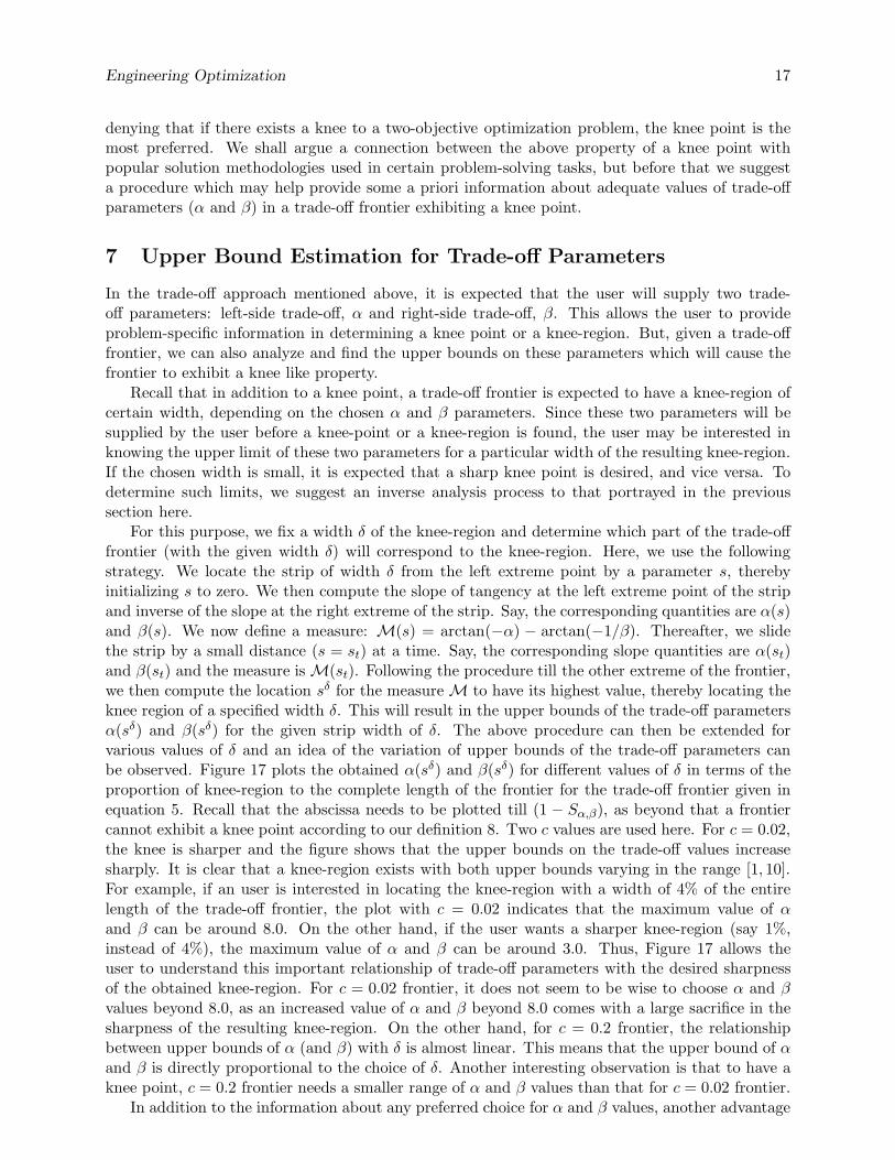
For this purpose, we fix a width δ of the knee-region and determine which part of the trade-offfrontier (with the given width δ) will correspond to the knee-region. Here, we use the followingstrategy. We locate the strip of width δ from the left extreme point by a parameter s, therebyinitializing s to zero. We then compute the slope of tangency at the left extreme point of the stripand inverse of the slope at the right extreme of the strip. Say, the corresponding quantities are α(s)and β(s). We now define a measure: M(s) = arctan(−α) − arctan(−1/β). Thereafter, we slidethe strip by a small distance (s = st) at a time. Say, the corresponding slope quantities are α(st)and β(st) and the measure is M(st). Following the procedure till the other extreme of the frontier,we then compute the location sδ for the measure M to have its highest value, thereby locating theknee region of a specified width δ. This will result in the upper bounds of the trade-off parametersα(sδ) and β(sδ) for the given strip width of δ. The above procedure can then be extended forvarious values of δ and an idea of the variation of upper bounds of the trade-off parameters canbe observed. Figure 17 plots the obtained α(sδ) and β(sδ) for different values of δ in terms of theproportion of knee-region to the complete length of the frontier for the trade-off frontier given inequation 5. Recall that the abscissa needs to be plotted till (1 − Sα,β), as beyond that a frontiercannot exhibit a knee point according to our definition 8. Two c values are used here. For c = 0.02,the knee is sharper and the figure shows that the upper bounds on the trade-off values increasesharply. It is clear that a knee-region exists with both upper bounds varying in the range [1, 10].For example, if an user is interested in locating the knee-region with a width of 4% of the entirelength of the trade-off frontier, the plot with c = 0.02 indicates that the maximum value of αand β can be around 8.0. On the other hand, if the user wants a sharper knee-region (say 1%,instead of 4%), the maximum value of α and β can be around 3.0. Thus, Figure 17 allows theuser to understand this important relationship of trade-off parameters with the desired sharpnessof the obtained knee-region. For c = 0.02 frontier, it does not seem to be wise to choose α and βvalues beyond 8.0, as an increased value of α and β beyond 8.0 comes with a large sacrifice in thesharpness of the resulting knee-region. On the other hand, for c = 0.2 frontier, the relationshipbetween upper bounds of α (and β) with δ is almost linear. This means that the upper bound of αand β is directly proportional to the choice of δ. Another interesting observation is that to have aknee point, c = 0.2 frontier needs a smaller range of α and β values than that for c = 0.02 frontier.
In addition to the information about any preferred choice for α and β values, another advantage
Engineering Optimization 18
Upp
er B
ound
of
c=0.2
c=0.02
3
4
5
6
7
8
9
10
0 0.02 0.04 0.06 0.08 0.1 0.12 0.14 0.16 0.18 0.2Proportion of Knee Region
βα
α, β
1
0
2
Figure 17: Obtained α and β values as a function of obtained proportion of knee-region.
of this analysis is that the user can estimate the width of the knee region a priori for a chosen upperbound of α and β values, thereby allowing the user to make a proper choice of trade-off parametersbefore looking for a knee or knee-line point in a trade-off frontier. We shall illustrate this analysistask for an engineering design problem later.
8 Problem-Solving Tasks and Knee Solutions
To discuss the connection between a knee point with preferred solution methodologies in certainproblem-solving tasks, let us consider the task of sorting a set of integers. The first methodologycomes to any mind is the quicksort procedure. There are two other methods – the bubble sortmethod which is the simplest and most straightforward sorting method and the binary-tree sortwhich is computationally the most efficient method. A plethora of other sorting algorithms exist,but an important question to ponder is when a sorting task is required why most researchersresort to the quicksort procedure. Next, let us consider the task of fitting a curve through a setof two-dimensional data points. Despite the existence of a dozen of different methods, why doresearchers prefer the polynomial regression method? Besides these generic problem-solving tasks,many engineering problems are found to have preferred solutions. For example, it is recommendedthat driving around 55 miles/hr is the most fuel-efficient approach, and so on.
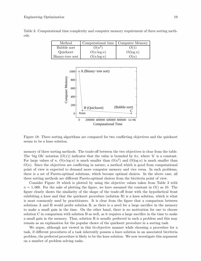
Could it be that the corresponding popular solution methodology or principle is an optimalsolution of a single goal of solving the problem. Let us consider the sorting example again. Anobvious goal any user is concerned about is the computational time. A method which takes thesmallest time to sort a set of numbers accurately is of interest to the user. But in such problem-solving tasks, a single objective is often not everything an user is interested. A method may befastest in computational time, but if it is very difficult to implement on a computer or if it takesa large amount of computer memory or if it has restricted application domain, the user may notbe interested in that method. Usually, in most problem-solving tasks, we can think of at least twoconflicting goals, both of which would of interest to an user. In the case of the sorting task, twoobjectives of minimizing computational time and computer memory would be conflicting to eachother. Table 3 presents the average-case computational time complexity and required computer
Engineering Optimization 19
Table 3: Computational time complexity and computer memory requirement of three sorting meth-ods.
Method Computational time Computer Memory
Bubble sort O(n2) O(1)Quicksort O(n log n) O(log n)
Binary-tree sort O(n log n) O(n)
(Bubble sort)C
Knee
A (Binary−tree sort)
B (Quicksort)
1000
0 200000 400000 600000
400
1e+06
Com
pute
r M
emor
y
Computational Time
200
0
800000
600
800
Figure 18: Three sorting algorithms are compared for two conflicting objectives and the quicksortseems to be a knee solution.
memory of three sorting methods. The trade-off between the two objectives is clear from the table.The ‘big Oh’ notation (O(x)) indicates that the value is bounded by kx, where ‘k’ is a constant.For large values of n, O(n log n) is much smaller than O(n2) and O(log n) is much smaller thanO(n). Since the objectives are conflicting in nature, a method which is good from computationalpoint of view is expected to demand more computer memory and vice versa. In such problems,there is a set of Pareto-optimal solutions, which become optimal choices. In the above case, allthree sorting methods are different Pareto-optimal choices from the bicriteria point of view.
Consider Figure 18 which is plotted by using the objective values taken from Table 3 withn = 1, 000. For the sake of plotting the figure, we have assumed the constant in O() as 10. Thefigure clearly shows the similarity of the shape of the trade-off front with the hypothetical frontexhibiting a knee and that the quicksort procedure (solution B) is a knee solution, which is whatis most commonly used by practitioners. It is clear from the figure that a comparison betweensolutions A and B would prefer solution B, as there is a need for a large sacrifice in the memoryto make a small gain in the time. On the other hand, there is no motivation for one to choosesolution C in comparison with solution B as well, as it requires a large sacrifice in the time to makea small gain in the memory. Thus, solution B is usually preferred in such a problem and this mayremain as an explanation for the popular choice of the quicksort procedure in a sorting task.
We argue, although not viewed in this bi-objective manner while choosing a procedure for atask, if different procedures of a task inherently possess a knee solution in an associated bicriteriaproblem, the preferred procedure is likely to be the knee solution. We now investigate this argumenton a number of problem solving tasks.
Engineering Optimization 20
9 Some Practical Problem-Solving Tasks
In this section, we take three different generic problem-solving tasks and four engineering designproblems from transportation to mechanical engineering design tasks to understand and analyzethe reasons for popularity of common solution methodologies from a bi-objective point of view.
9.1 Bucket Sorting Procedure
We have considered the sorting problem above, purely from the reported computational time andmemory requirement of three sorting methodologies. There exist a number of sorting algorithmswith differences in performance in terms of computational complexity, memory usage, and stability.For some algorithms, average and worst-case quantities of the performance indicators are workedout, but their actual values depend on the data set being considered.
In this section, we consider the bucket sorting algorithm the performance of which can becontrolled by using a parameter, called the bucket size d. In this algorithm, all numbers aredivided into d buckets, each bucket with an equal range of values. Each bucket is then sortedusing the Insertion Sort procedure. Let us assume that there are ‘n’ numbers that needs to besorted. Then, the space complexity is given by O(2n + d), of which the output takes O(n) space,the buckets in which individual numbers are stored takes up a total of O(
∑
di) (=O(n)) space anda vector that keeps the count of the number of elements present in the buckets will have a size ofO(d). The time complexity is calculated as follows: O(n), time is required to scan the data setand place each number into it’s corresponding bucket, O(1) time is required for each call made toinsertion sort which sorts the numbers in a bucket, and O(1) time is required for each swap madein the insertion sort. Although these numbers give an indication of their orders of magnitude asa function of size of data set(n) and the number of buckets(d), the actual implementation mayproduce different results (depending upon the data set).
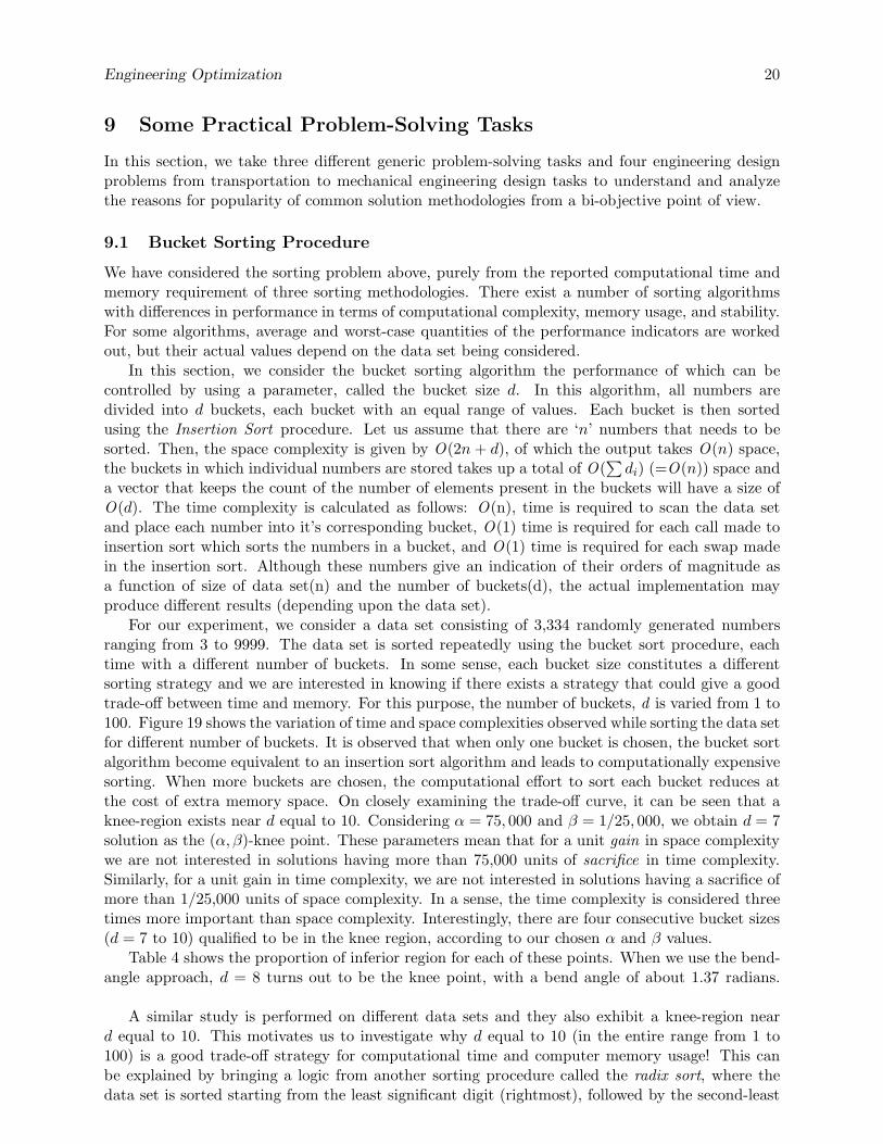
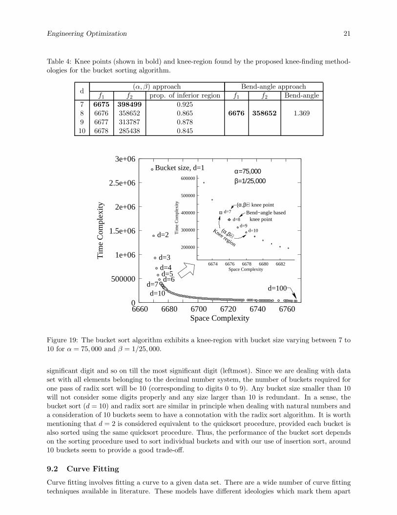
For our experiment, we consider a data set consisting of 3,334 randomly generated numbersranging from 3 to 9999. The data set is sorted repeatedly using the bucket sort procedure, eachtime with a different number of buckets. In some sense, each bucket size constitutes a differentsorting strategy and we are interested in knowing if there exists a strategy that could give a goodtrade-off between time and memory. For this purpose, the number of buckets, d is varied from 1 to100. Figure 19 shows the variation of time and space complexities observed while sorting the data setfor different number of buckets. It is observed that when only one bucket is chosen, the bucket sortalgorithm become equivalent to an insertion sort algorithm and leads to computationally expensivesorting. When more buckets are chosen, the computational effort to sort each bucket reduces atthe cost of extra memory space. On closely examining the trade-off curve, it can be seen that aknee-region exists near d equal to 10. Considering α = 75, 000 and β = 1/25, 000, we obtain d = 7solution as the (α, β)-knee point. These parameters mean that for a unit gain in space complexitywe are not interested in solutions having more than 75,000 units of sacrifice in time complexity.Similarly, for a unit gain in time complexity, we are not interested in solutions having a sacrifice ofmore than 1/25,000 units of space complexity. In a sense, the time complexity is considered threetimes more important than space complexity. Interestingly, there are four consecutive bucket sizes(d = 7 to 10) qualified to be in the knee region, according to our chosen α and β values.
Table 4 shows the proportion of inferior region for each of these points. When we use the bend-angle approach, d = 8 turns out to be the knee point, with a bend angle of about 1.37 radians.
A similar study is performed on different data sets and they also exhibit a knee-region neard equal to 10. This motivates us to investigate why d equal to 10 (in the entire range from 1 to100) is a good trade-off strategy for computational time and computer memory usage! This canbe explained by bringing a logic from another sorting procedure called the radix sort, where thedata set is sorted starting from the least significant digit (rightmost), followed by the second-least
Engineering Optimization 21
Table 4: Knee points (shown in bold) and knee-region found by the proposed knee-finding method-ologies for the bucket sorting algorithm.
d(α, β) approach Bend-angle approach
f1 f2 prop. of inferior region f1 f2 Bend-angle
7 6675 398499 0.9258 6676 358652 0.865 6676 358652 1.3699 6677 313787 0.87810 6678 285438 0.845
d=10d=7
(α,β)−Knee region
β=1/25,000α=75,000
knee pointBend−angle based
knee point(α,β)−d=7
d=10d=9
d=8
Bucket size, d=1
d=2
d=100
d=5d=6
d=4d=3
500000
1e+06
1.5e+06
2e+06
2.5e+06
3e+06
6660 6680 6700 6720 6740 6760
Tim
e C
ompl
exity
Space Complexity
6674 6676 6678 6680 6682
Tim
e C
ompl
exity
Space Complexity
200000
300000
400000
500000
0
600000
Figure 19: The bucket sort algorithm exhibits a knee-region with bucket size varying between 7 to10 for α = 75, 000 and β = 1/25, 000.
significant digit and so on till the most significant digit (leftmost). Since we are dealing with dataset with all elements belonging to the decimal number system, the number of buckets required forone pass of radix sort will be 10 (corresponding to digits 0 to 9). Any bucket size smaller than 10will not consider some digits properly and any size larger than 10 is redundant. In a sense, thebucket sort (d = 10) and radix sort are similar in principle when dealing with natural numbers anda consideration of 10 buckets seem to have a connotation with the radix sort algorithm. It is worthmentioning that d = 2 is considered equivalent to the quicksort procedure, provided each bucket isalso sorted using the same quicksort procedure. Thus, the performance of the bucket sort dependson the sorting procedure used to sort individual buckets and with our use of insertion sort, around10 buckets seem to provide a good trade-off.
9.2 Curve Fitting
Curve fitting involves fitting a curve to a given data set. There are a wide number of curve fittingtechniques available in literature. These models have different ideologies which mark them apart
Engineering Optimization 22
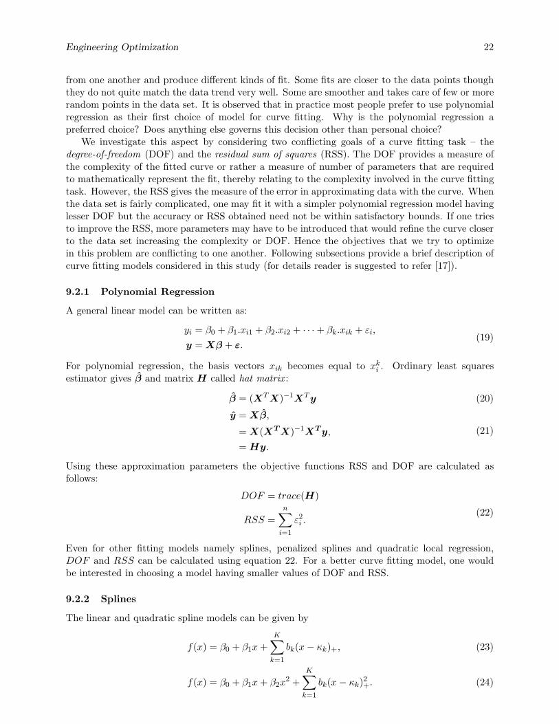
from one another and produce different kinds of fit. Some fits are closer to the data points thoughthey do not quite match the data trend very well. Some are smoother and takes care of few or morerandom points in the data set. It is observed that in practice most people prefer to use polynomialregression as their first choice of model for curve fitting. Why is the polynomial regression apreferred choice? Does anything else governs this decision other than personal choice?
We investigate this aspect by considering two conflicting goals of a curve fitting task – thedegree-of-freedom (DOF) and the residual sum of squares (RSS). The DOF provides a measure ofthe complexity of the fitted curve or rather a measure of number of parameters that are requiredto mathematically represent the fit, thereby relating to the complexity involved in the curve fittingtask. However, the RSS gives the measure of the error in approximating data with the curve. Whenthe data set is fairly complicated, one may fit it with a simpler polynomial regression model havinglesser DOF but the accuracy or RSS obtained need not be within satisfactory bounds. If one triesto improve the RSS, more parameters may have to be introduced that would refine the curve closerto the data set increasing the complexity or DOF. Hence the objectives that we try to optimizein this problem are conflicting to one another. Following subsections provide a brief description ofcurve fitting models considered in this study (for details reader is suggested to refer [17]).
9.2.1 Polynomial Regression
A general linear model can be written as:
yi = β0 + β1.xi1 + β2.xi2 + · · · + βk.xik + εi,
y = Xβ + ε.(19)
For polynomial regression, the basis vectors xik becomes equal to xki . Ordinary least squares
estimator gives β and matrix H called hat matrix :
β = (XT X)−1XT y (20)
y = Xβ,
= X(XT X)−1XTy,
= Hy.
(21)
Using these approximation parameters the objective functions RSS and DOF are calculated asfollows:
DOF = trace(H)
RSS =
n∑
i=1
ε2i .
(22)
Even for other fitting models namely splines, penalized splines and quadratic local regression,DOF and RSS can be calculated using equation 22. For a better curve fitting model, one wouldbe interested in choosing a model having smaller values of DOF and RSS.
9.2.2 Splines
The linear and quadratic spline models can be given by
f(x) = β0 + β1x +
K∑
k=1
bk(x − κk)+, (23)
f(x) = β0 + β1x + β2x2 +
K∑
k=1
bk(x − κk)2+. (24)
Engineering Optimization 23
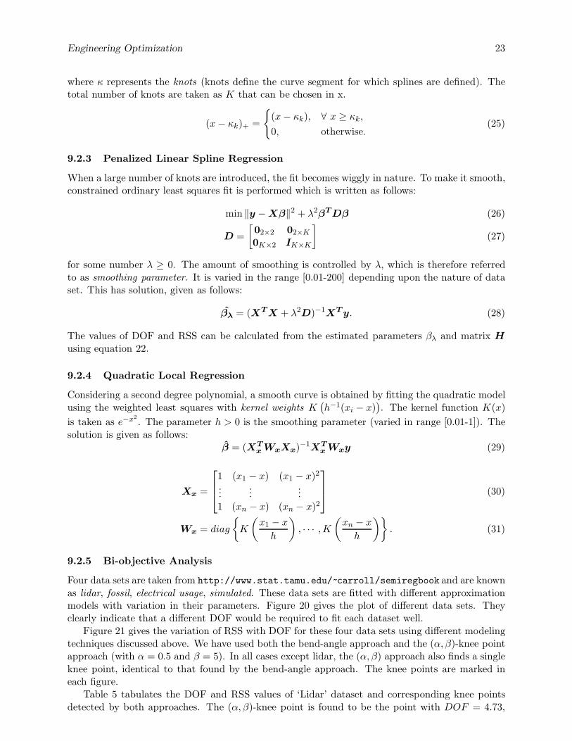
where κ represents the knots (knots define the curve segment for which splines are defined). Thetotal number of knots are taken as K that can be chosen in x.
(x − κk)+ =
{
(x − κk), ∀ x ≥ κk,
0, otherwise.(25)
9.2.3 Penalized Linear Spline Regression
When a large number of knots are introduced, the fit becomes wiggly in nature. To make it smooth,constrained ordinary least squares fit is performed which is written as follows:
min ‖y − Xβ‖2 + λ2βTDβ (26)
D =
[
02×2 02×K
0K×2 IK×K
]
(27)
for some number λ ≥ 0. The amount of smoothing is controlled by λ, which is therefore referredto as smoothing parameter. It is varied in the range [0.01-200] depending upon the nature of dataset. This has solution, given as follows:
βλ = (XT X + λ2D)−1XT y. (28)
The values of DOF and RSS can be calculated from the estimated parameters βλ and matrix H
using equation 22.
9.2.4 Quadratic Local Regression
Considering a second degree polynomial, a smooth curve is obtained by fitting the quadratic modelusing the weighted least squares with kernel weights K
(
h−1(xi − x))
. The kernel function K(x)
is taken as e−x2
. The parameter h > 0 is the smoothing parameter (varied in range [0.01-1]). Thesolution is given as follows:
β = (XT
x WxXx)−1XT
x Wxy (29)
Xx =
1 (x1 − x) (x1 − x)2
......
...1 (xn − x) (xn − x)2
(30)
Wx = diag
{
K
(
x1 − x
h
)
, · · · ,K
(
xn − x
h
)}
. (31)
9.2.5 Bi-objective Analysis
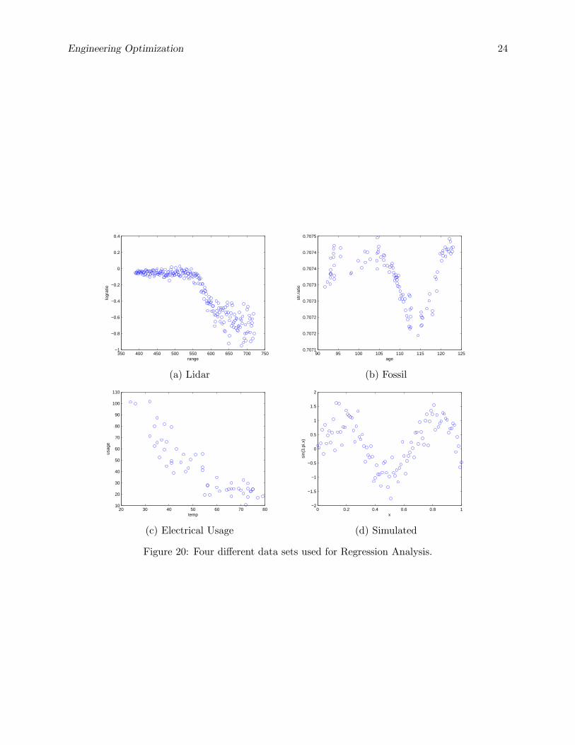
Four data sets are taken from http://www.stat.tamu.edu/~carroll/semiregbook and are knownas lidar, fossil, electrical usage, simulated. These data sets are fitted with different approximationmodels with variation in their parameters. Figure 20 gives the plot of different data sets. Theyclearly indicate that a different DOF would be required to fit each dataset well.
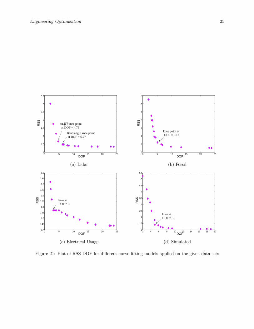
Figure 21 gives the variation of RSS with DOF for these four data sets using different modelingtechniques discussed above. We have used both the bend-angle approach and the (α, β)-knee pointapproach (with α = 0.5 and β = 5). In all cases except lidar, the (α, β) approach also finds a singleknee point, identical to that found by the bend-angle approach. The knee points are marked ineach figure.
Table 5 tabulates the DOF and RSS values of ‘Lidar’ dataset and corresponding knee pointsdetected by both approaches. The (α, β)-knee point is found to be the point with DOF = 4.73,
Engineering Optimization 24
350 400 450 500 550 600 650 700 750−1
−0.8
−0.6
−0.4
−0.2
0
0.2
0.4
range
logr
atio
90 95 100 105 110 115 120 1250.7071
0.7072
0.7072
0.7073
0.7073
0.7074
0.7074
0.7075
age
str.
ratio
(a) Lidar (b) Fossil
20 30 40 50 60 70 8010
20
30
40
50
60
70
80
90
100
110
temp
usag
e
0 0.2 0.4 0.6 0.8 1−2
−1.5
−1
−0.5
0
0.5
1
1.5
2
x
sin(
3.pi
.x)
(c) Electrical Usage (d) Simulated
Figure 20: Four different data sets used for Regression Analysis.
Engineering Optimization 25
0 5 10 15 20 251
1.5
2
2.5
3
3.5
4
4.5
DOF
RS
S
Bend angle knee pointat DOF = 6.27
at DOF = 4.73(α,β)−knee point
0 5 10 15 20 250
1
2
3
4
5
6
7
DOF
RS
S
knee point atDOF = 5.12
(a) Lidar (b) Fossil
0 5 10 15 20 250.4
0.45
0.5
0.55
0.6
0.65
0.7
0.75
0.8
0.85
0.9
DOF
RS
S
DOF = 3knee at
2 4 6 8 10 12 14 16 18 201
1.5
2
2.5
3
3.5
4
4.5
5
5.5
DOF
RS
S
DOF = 5knee at
(c) Electrical Usage (d) Simulated
Figure 21: Plot of RSS-DOF for different curve fitting models applied on the given data sets

Engineering Optimization 26
Table 5: Knee points (shown in bold) found by the proposed methodologies on ‘Lidar’ dataset. Thefourth point is declared a knee point by the (α, β) approach and the fifth point is by bend-angleapproach.
Curve Fitting Model DOF RSSProp. of
Bend-angleInferior Region
Linear Reg. 2.00 4.00Poly. Reg. (2nd order) 3.00 2.75 0.749 0.969Poly. Reg. (3rd order) 4.00 2.15 0.879 1.121Pen. Linear Spline (λ = 200) 4.73 1.68 1.000 1.289Pen. Linear Spline (λ = 100) 6.27 1.50 0.844 1.298
Quadratic Local Reg. (h = 0.1) 6.63 1.49 0.828 1.285Quadratic Local Reg. (h = 0.08) 7.89 1.44 0.703 1.254Pen. Linear Spline (λ = 50) 8.44 1.42 0.679 1.241Pen. Linear Spline (λ = 30) 10.55 1.39 0.587 1.170Quadratic Local Reg. (h = 0.05) 11.68 1.38 0.538 1.132Pen. Linear Spline (λ = 10) 16.34 1.37 0.334 0.968Quadratic Local Reg. (h = 0.03) 18.42 1.36 0.243 0.913Linear Spline 23.00 1.35 0.044 0.809Quadratic Spline 24.00 1.35
close to polynomial regression with a fourth-order polynomial, whereas the bend-angle approachfinds the regression with a DOF = 6.27 – close to fifth-order polynomial. Figure 21(a) shows thatthese two points on the objective space are close to each other and are visually likely to be a kneepoint.
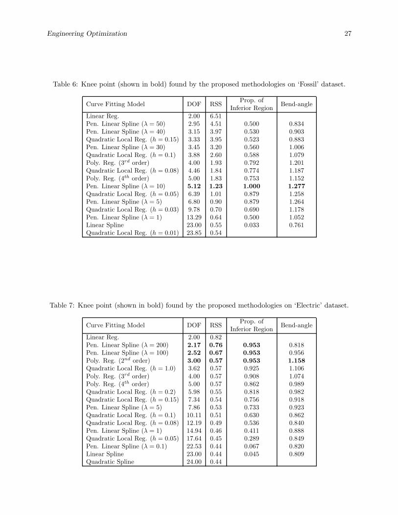
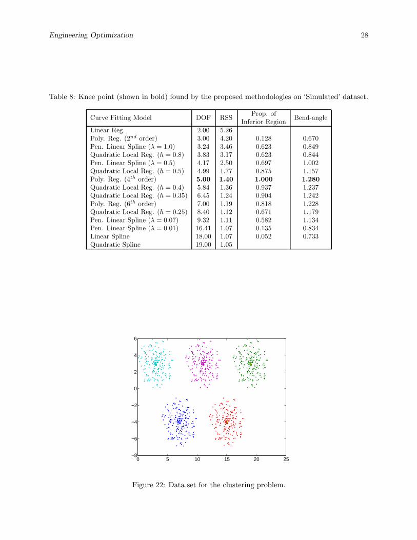
For the ‘Fossil’ dataset, the knee point is obtained at DOF = 5.12 using both (α, β) and bendangle approach. This is close to a fourth-order polynomial regression (Table 6). For the ‘Electric’data-set (Table 7), there are three regression approaches (penalized linear spline with λ = 100 and200, and the polynomial regression of order two) that have maximum proportion of inferior regionwith the chosen α and β values. In principle, any of these three approaches can be consideredas a knee solution, however, if a smaller α value is chosen, the polynomial regression of order twobecomes the knee solution. For the the ‘Simulated’ data-set (Table 8), the knee points occur exactlyat DOF = 5 by both approaches. It is interesting that both approaches of defining a knee pointprovide similar outcomes to all the four datasets,
It is also clear from the plots that polynomial regression points are clustered around the kneepoint, indicating that polynomial regression with DOF ∈ [3, 6], in general, provides a good trade-off between computational complexity and obtained error of regression. Based on this finding, weargue that this can be one of the reasons why researchers prefer polynomial regression with a smallDOF.
9.3 Data Clustering
Clustering is a widely-used computational task in almost any field of science and engineering.Researchers have preferences of one clustering algorithm over another. In many clustering problems,the number of clusters is usually not known beforehand and the part of the clustering task is alsoto determine how many clusters is optimum for the given data set. Here, we consider a simple dataset, which can be visually clustered into a set of five clusters. Figure 22 shows the data set. Insteadof trying different clustering algorithms, here, we use the well-known k-mean clustering algorithmand keep the number of cluster as a parameter. Thus, when p clusters are fixed in the clusteringalgorithm, the algorithm is called p-clustering algorithm, denoting that this specific algorithm canonly cluster points data sets into p different clusters.
Engineering Optimization 27
Table 6: Knee point (shown in bold) found by the proposed methodologies on ‘Fossil’ dataset.
Curve Fitting Model DOF RSSProp. of
Bend-angleInferior Region
Linear Reg. 2.00 6.51Pen. Linear Spline (λ = 50) 2.95 4.51 0.500 0.834Pen. Linear Spline (λ = 40) 3.15 3.97 0.530 0.903Quadratic Local Reg. (h = 0.15) 3.33 3.95 0.523 0.883Pen. Linear Spline (λ = 30) 3.45 3.20 0.560 1.006Quadratic Local Reg. (h = 0.1) 3.88 2.60 0.588 1.079Poly. Reg. (3rd order) 4.00 1.93 0.792 1.201Quadratic Local Reg. (h = 0.08) 4.46 1.84 0.774 1.187Poly. Reg. (4th order) 5.00 1.83 0.753 1.152Pen. Linear Spline (λ = 10) 5.12 1.23 1.000 1.277
Quadratic Local Reg. (h = 0.05) 6.39 1.01 0.879 1.258Pen. Linear Spline (λ = 5) 6.80 0.90 0.879 1.264Quadratic Local Reg. (h = 0.03) 9.78 0.70 0.690 1.178Pen. Linear Spline (λ = 1) 13.29 0.64 0.500 1.052Linear Spline 23.00 0.55 0.033 0.761Quadratic Local Reg. (h = 0.01) 23.85 0.54
Table 7: Knee point (shown in bold) found by the proposed methodologies on ‘Electric’ dataset.
Curve Fitting Model DOF RSSProp. of
Bend-angleInferior Region
Linear Reg. 2.00 0.82Pen. Linear Spline (λ = 200) 2.17 0.76 0.953 0.818Pen. Linear Spline (λ = 100) 2.52 0.67 0.953 0.956Poly. Reg. (2nd order) 3.00 0.57 0.953 1.158
Quadratic Local Reg. (h = 1.0) 3.62 0.57 0.925 1.106Poly. Reg. (3rd order) 4.00 0.57 0.908 1.074Poly. Reg. (4th order) 5.00 0.57 0.862 0.989Quadratic Local Reg. (h = 0.2) 5.98 0.55 0.818 0.982Quadratic Local Reg. (h = 0.15) 7.34 0.54 0.756 0.918Pen. Linear Spline (λ = 5) 7.86 0.53 0.733 0.923Quadratic Local Reg. (h = 0.1) 10.11 0.51 0.630 0.862Quadratic Local Reg. (h = 0.08) 12.19 0.49 0.536 0.840Pen. Linear Spline (λ = 1) 14.94 0.46 0.411 0.888Quadratic Local Reg. (h = 0.05) 17.64 0.45 0.289 0.849Pen. Linear Spline (λ = 0.1) 22.53 0.44 0.067 0.820Linear Spline 23.00 0.44 0.045 0.809Quadratic Spline 24.00 0.44
Engineering Optimization 28
Table 8: Knee point (shown in bold) found by the proposed methodologies on ‘Simulated’ dataset.
Curve Fitting Model DOF RSSProp. of
Bend-angleInferior Region
Linear Reg. 2.00 5.26Poly. Reg. (2nd order) 3.00 4.20 0.128 0.670Pen. Linear Spline (λ = 1.0) 3.24 3.46 0.623 0.849Quadratic Local Reg. (h = 0.8) 3.83 3.17 0.623 0.844Pen. Linear Spline (λ = 0.5) 4.17 2.50 0.697 1.002Quadratic Local Reg. (h = 0.5) 4.99 1.77 0.875 1.157Poly. Reg. (4th order) 5.00 1.40 1.000 1.280
Quadratic Local Reg. (h = 0.4) 5.84 1.36 0.937 1.237Quadratic Local Reg. (h = 0.35) 6.45 1.24 0.904 1.242Poly. Reg. (6th order) 7.00 1.19 0.818 1.228Quadratic Local Reg. (h = 0.25) 8.40 1.12 0.671 1.179Pen. Linear Spline (λ = 0.07) 9.32 1.11 0.582 1.134Pen. Linear Spline (λ = 0.01) 16.41 1.07 0.135 0.834Linear Spline 18.00 1.07 0.052 0.733Quadratic Spline 19.00 1.05
0 5 10 15 20 25−8
−6
−4
−2
0
2
4
6
Figure 22: Data set for the clustering problem.
Engineering Optimization 29
p=10p=15
p=2
p=5p=7
Knee point
4000
4500
5000
0.1 0.15 0.2 0.25 0.3
1500
0.4 0.45 0.5 0.55
Ove
rall
Dev
iatio
n
Connectivity
1000 0.35
2000
2500
3000
3500
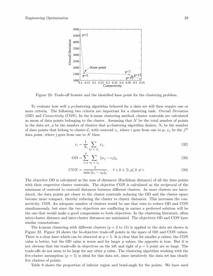
Figure 23: Trade-off frontier and the identified knee point for the clustering problem.
To evaluate how well a p-clustering algorithm behaved for a data set will then require one ormore criteria. The following two criteria are important for a clustering task: Overall Deviation(OD) and Connectivity (CON). In the k-mean clustering method, cluster centroids are calculatedas mean of data points belonging to the cluster. Assuming that N be the total number of pointsin the data set, p be the number of clusters that p-clustering algorithm desires, Ni be the numberof data points that belong to cluster Ci with centroid ci, where i goes from one to p, xj be the jth
data point, where j goes from one to N then:
ci =1
Ni
∑
∀j ∈ Ci
xj, (32)
OD =
p∑
i=1
∑
∀j ∈ Ci
‖xj − ci‖2, (33)
CON =1
min ‖ci − ck‖2, ∀ i, k ∈ [1, p], k 6= i. (34)
The objective OD is calculated as the sum of distances (Euclidean distance) of all the data pointswith their respective cluster centroids. The objective CON is calculated as the reciprocal of theminimum of centroid to centroid distances between different clusters. As more clusters are intro-duced, the data points get closer to the cluster centroids reducing the OD and the cluster spacebecome more compact, thereby reducing the cluster to cluster distances. This increases the con-nectivity, CON. An adequate number of clusters would be one that tries to reduce OD and CONsimultaneously, but since the two objectives are conflicting in nature a preferred solution will bethe one that would make a good compromise to both objectives. In the clustering literature, oftenintra-cluster distance and inter-cluster distances are minimized. The objectives OD and CON havesimilar connotations.
The k-mean clustering with different clusters (p = 2 to 15) is applied to the data set shown inFigure 22. Figure 23 shows the bi-objective trade-off points in the space of OD and CON values.There is a clear knee which can be observed at p = 5. It is clear that for smaller p values, the CONvalue is better, but the OD value is worse and for larger p values, the opposite is true. But it isnot obvious that the trade-offs in objectives on the left and right of p = 5 point are so large. Thetrade-offs do not seem to be large for any other p value. The clustering algorithm working with thefive-cluster assumption (p = 5) is ideal for this data set, since intuitively the data set has clearlyfive clusters of points.
Table 9 shows the proportion of inferior region and bend-angle for the points. We have used
Engineering Optimization 30
Table 9: Knee point (shown in bold) found by the proposed methodologies on the clustering dataset.
p Connectivity Deviation prop. of inferior region Bend-angle
2 0.10 4523.905 0.13 1576.70 1.000 1.349
7 0.46 1456.50 0.099 0.33610 0.48 1331.50 0.062 0.39915 0.54 1120.20
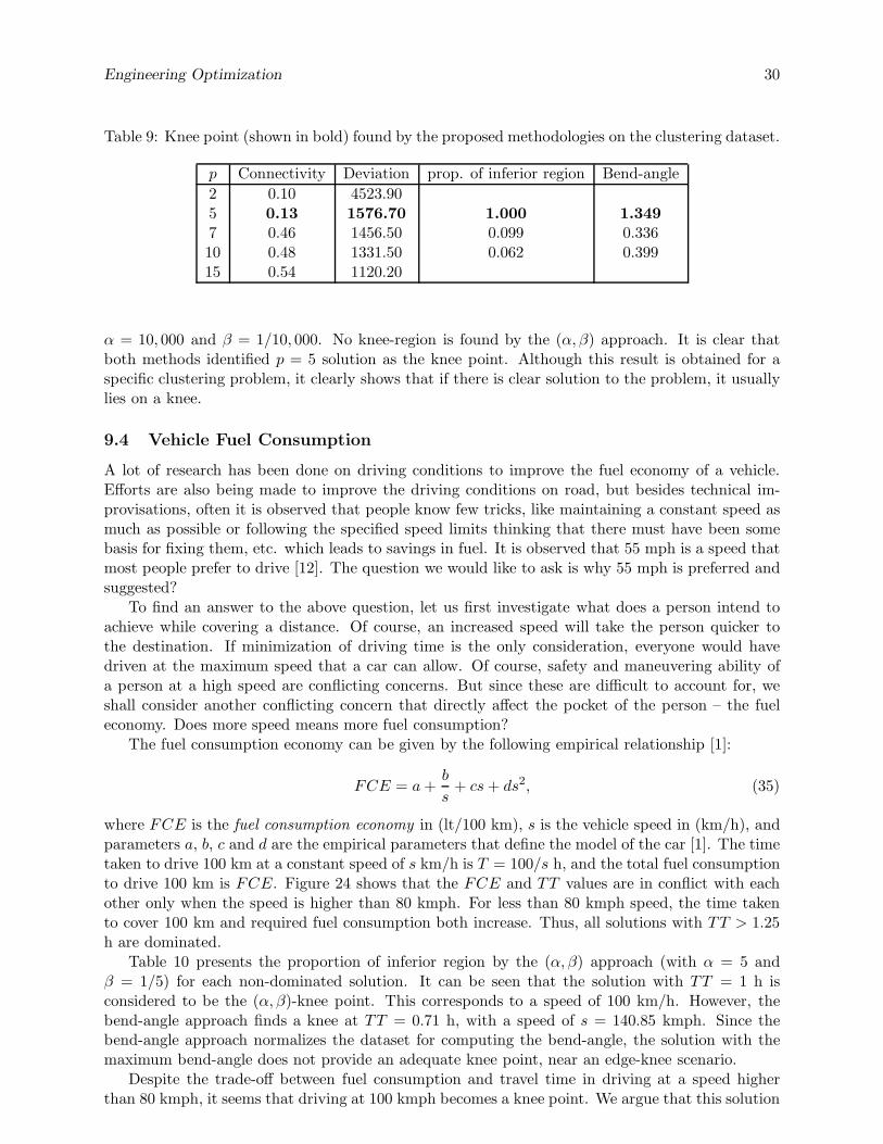
α = 10, 000 and β = 1/10, 000. No knee-region is found by the (α, β) approach. It is clear thatboth methods identified p = 5 solution as the knee point. Although this result is obtained for aspecific clustering problem, it clearly shows that if there is clear solution to the problem, it usuallylies on a knee.
9.4 Vehicle Fuel Consumption
A lot of research has been done on driving conditions to improve the fuel economy of a vehicle.Efforts are also being made to improve the driving conditions on road, but besides technical im-provisations, often it is observed that people know few tricks, like maintaining a constant speed asmuch as possible or following the specified speed limits thinking that there must have been somebasis for fixing them, etc. which leads to savings in fuel. It is observed that 55 mph is a speed thatmost people prefer to drive [12]. The question we would like to ask is why 55 mph is preferred andsuggested?
To find an answer to the above question, let us first investigate what does a person intend toachieve while covering a distance. Of course, an increased speed will take the person quicker tothe destination. If minimization of driving time is the only consideration, everyone would havedriven at the maximum speed that a car can allow. Of course, safety and maneuvering ability ofa person at a high speed are conflicting concerns. But since these are difficult to account for, weshall consider another conflicting concern that directly affect the pocket of the person – the fueleconomy. Does more speed means more fuel consumption?
The fuel consumption economy can be given by the following empirical relationship [1]:
FCE = a +b
s+ cs + ds2, (35)
where FCE is the fuel consumption economy in (lt/100 km), s is the vehicle speed in (km/h), andparameters a, b, c and d are the empirical parameters that define the model of the car [1]. The timetaken to drive 100 km at a constant speed of s km/h is T = 100/s h, and the total fuel consumptionto drive 100 km is FCE. Figure 24 shows that the FCE and TT values are in conflict with eachother only when the speed is higher than 80 kmph. For less than 80 kmph speed, the time takento cover 100 km and required fuel consumption both increase. Thus, all solutions with TT > 1.25h are dominated.
Table 10 presents the proportion of inferior region by the (α, β) approach (with α = 5 andβ = 1/5) for each non-dominated solution. It can be seen that the solution with TT = 1 h isconsidered to be the (α, β)-knee point. This corresponds to a speed of 100 km/h. However, thebend-angle approach finds a knee at TT = 0.71 h, with a speed of s = 140.85 kmph. Since thebend-angle approach normalizes the dataset for computing the bend-angle, the solution with themaximum bend-angle does not provide an adequate knee point, near an edge-knee scenario.
Despite the trade-off between fuel consumption and travel time in driving at a speed higherthan 80 kmph, it seems that driving at 100 kmph becomes a knee point. We argue that this solution
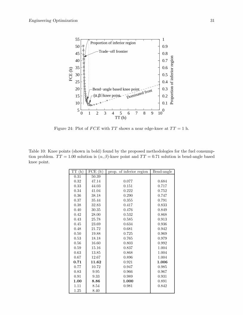
Engineering Optimization 31
Trade−off frontier
Proportion of inferior region
Dominated front
−knee point(α,β)Bend−angle based knee point
Pro
port
ion
of in
ferio
r re
gion
TT (h) 0 1 2 3
0.1
0.2
0.3
0.4
0.5
0.6
0.7
4 5 6 7 8 9 10 0 5
10
15
20
25
30
35
40
45
50
0.8
0.9
55
FC
E (
lt)
1
Figure 24: Plot of FCE with TT shows a near edge-knee at TT = 1 h.
Table 10: Knee points (shown in bold) found by the proposed methodologies for the fuel consump-tion problem. TT = 1.00 solution is (α, β)-knee point and TT = 0.71 solution is bend-angle basedknee point.
TT (h) FCE (lt) prop. of inferior region Bend-angle0.31 50.390.32 47.14 0.077 0.6840.33 44.03 0.151 0.7170.34 41.04 0.222 0.7520.36 38.18 0.290 0.7470.37 35.44 0.355 0.7910.38 32.83 0.417 0.8330.40 30.35 0.476 0.8490.42 28.00 0.532 0.8680.43 25.78 0.585 0.9130.45 23.69 0.634 0.9360.48 21.72 0.681 0.9420.50 19.88 0.725 0.9690.53 18.18 0.765 0.9790.56 16.60 0.803 0.9920.59 15.16 0.837 1.0040.63 13.85 0.868 1.0040.67 12.67 0.896 1.0040.71 11.62 0.921 1.006
0.77 10.72 0.947 0.9850.83 9.95 0.966 0.9670.91 9.33 0.989 0.9311.00 8.86 1.000 0.8911.11 8.54 0.981 0.8421.25 8.40
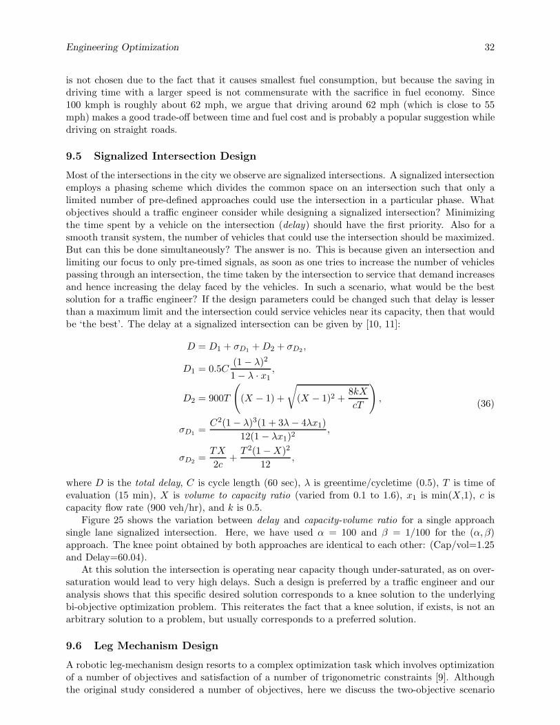
Engineering Optimization 32
is not chosen due to the fact that it causes smallest fuel consumption, but because the saving indriving time with a larger speed is not commensurate with the sacrifice in fuel economy. Since100 kmph is roughly about 62 mph, we argue that driving around 62 mph (which is close to 55mph) makes a good trade-off between time and fuel cost and is probably a popular suggestion whiledriving on straight roads.
9.5 Signalized Intersection Design
Most of the intersections in the city we observe are signalized intersections. A signalized intersectionemploys a phasing scheme which divides the common space on an intersection such that only alimited number of pre-defined approaches could use the intersection in a particular phase. Whatobjectives should a traffic engineer consider while designing a signalized intersection? Minimizingthe time spent by a vehicle on the intersection (delay) should have the first priority. Also for asmooth transit system, the number of vehicles that could use the intersection should be maximized.But can this be done simultaneously? The answer is no. This is because given an intersection andlimiting our focus to only pre-timed signals, as soon as one tries to increase the number of vehiclespassing through an intersection, the time taken by the intersection to service that demand increasesand hence increasing the delay faced by the vehicles. In such a scenario, what would be the bestsolution for a traffic engineer? If the design parameters could be changed such that delay is lesserthan a maximum limit and the intersection could service vehicles near its capacity, then that wouldbe ‘the best’. The delay at a signalized intersection can be given by [10, 11]:
D = D1 + σD1+ D2 + σD2
,
D1 = 0.5C(1 − λ)2
1 − λ · x1,
D2 = 900T
(
(X − 1) +
√
(X − 1)2 +8kX
cT
)
,
σD1=
C2(1 − λ)3(1 + 3λ − 4λx1)
12(1 − λx1)2,
σD2=
TX
2c+
T 2(1 − X)2
12,
(36)
where D is the total delay, C is cycle length (60 sec), λ is greentime/cycletime (0.5), T is time ofevaluation (15 min), X is volume to capacity ratio (varied from 0.1 to 1.6), x1 is min(X,1), c iscapacity flow rate (900 veh/hr), and k is 0.5.
Figure 25 shows the variation between delay and capacity-volume ratio for a single approachsingle lane signalized intersection. Here, we have used α = 100 and β = 1/100 for the (α, β)approach. The knee point obtained by both approaches are identical to each other: (Cap/vol=1.25and Delay=60.04).
At this solution the intersection is operating near capacity though under-saturated, as on over-saturation would lead to very high delays. Such a design is preferred by a traffic engineer and ouranalysis shows that this specific desired solution corresponds to a knee solution to the underlyingbi-objective optimization problem. This reiterates the fact that a knee solution, if exists, is not anarbitrary solution to a problem, but usually corresponds to a preferred solution.
9.6 Leg Mechanism Design
A robotic leg-mechanism design resorts to a complex optimization task which involves optimizationof a number of objectives and satisfaction of a number of trigonometric constraints [9]. Althoughthe original study considered a number of objectives, here we discuss the two-objective scenario
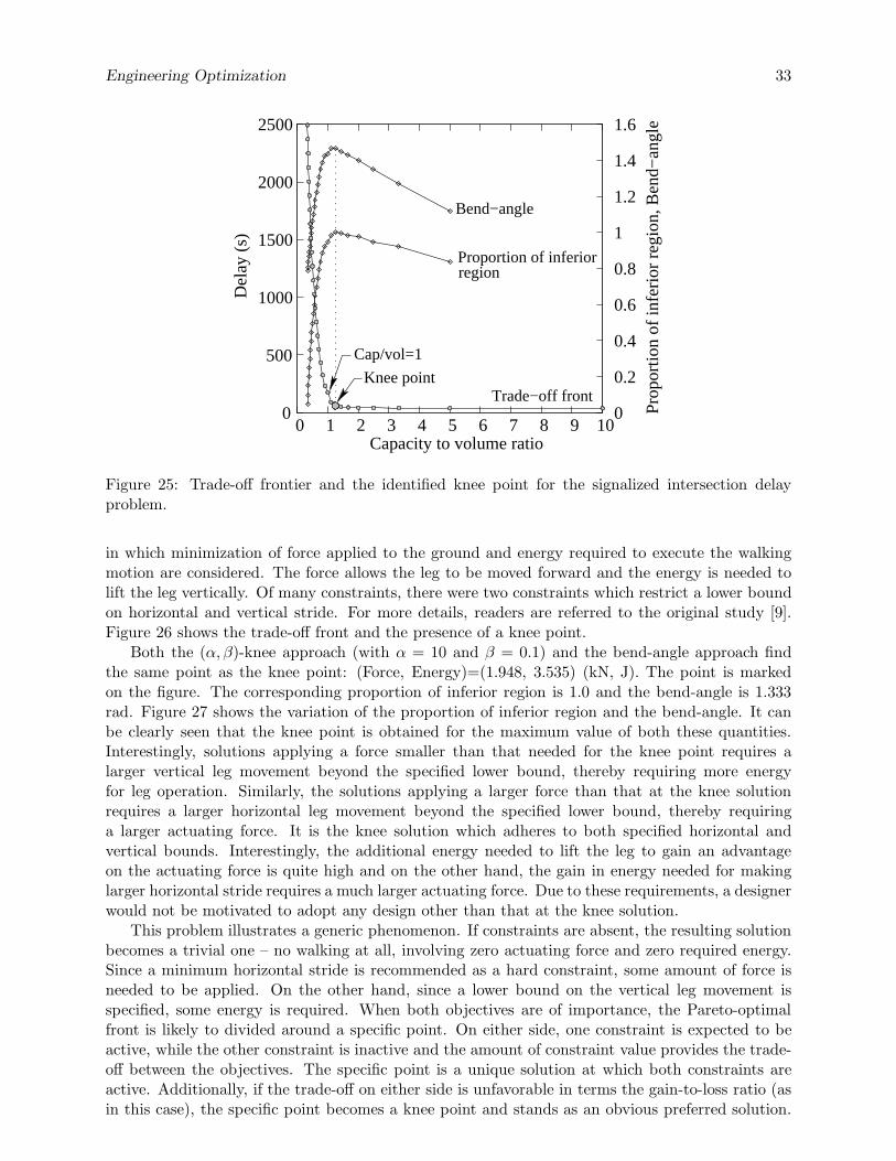
Engineering Optimization 33
Bend−angle
region
Trade−off front
Cap/vol=1
Knee point
Proportion of inferior
Pro
port
ion
of in
ferio
r re
gion
, Ben
d−an
gle
0
500
1000
1500
2000
2500
0 1 2 3 4 5 6 7 8 9 10 0
0.2
0.4
0.6
0.8
1
1.2
1.4
1.6
Del
ay (
s)
Capacity to volume ratio
Figure 25: Trade-off frontier and the identified knee point for the signalized intersection delayproblem.
in which minimization of force applied to the ground and energy required to execute the walkingmotion are considered. The force allows the leg to be moved forward and the energy is needed tolift the leg vertically. Of many constraints, there were two constraints which restrict a lower boundon horizontal and vertical stride. For more details, readers are referred to the original study [9].Figure 26 shows the trade-off front and the presence of a knee point.
Both the (α, β)-knee approach (with α = 10 and β = 0.1) and the bend-angle approach findthe same point as the knee point: (Force, Energy)=(1.948, 3.535) (kN, J). The point is markedon the figure. The corresponding proportion of inferior region is 1.0 and the bend-angle is 1.333rad. Figure 27 shows the variation of the proportion of inferior region and the bend-angle. It canbe clearly seen that the knee point is obtained for the maximum value of both these quantities.Interestingly, solutions applying a force smaller than that needed for the knee point requires alarger vertical leg movement beyond the specified lower bound, thereby requiring more energyfor leg operation. Similarly, the solutions applying a larger force than that at the knee solutionrequires a larger horizontal leg movement beyond the specified lower bound, thereby requiringa larger actuating force. It is the knee solution which adheres to both specified horizontal andvertical bounds. Interestingly, the additional energy needed to lift the leg to gain an advantageon the actuating force is quite high and on the other hand, the gain in energy needed for makinglarger horizontal stride requires a much larger actuating force. Due to these requirements, a designerwould not be motivated to adopt any design other than that at the knee solution.
This problem illustrates a generic phenomenon. If constraints are absent, the resulting solutionbecomes a trivial one – no walking at all, involving zero actuating force and zero required energy.Since a minimum horizontal stride is recommended as a hard constraint, some amount of force isneeded to be applied. On the other hand, since a lower bound on the vertical leg movement isspecified, some energy is required. When both objectives are of importance, the Pareto-optimalfront is likely to divided around a specific point. On either side, one constraint is expected to beactive, while the other constraint is inactive and the amount of constraint value provides the trade-off between the objectives. The specific point is a unique solution at which both constraints areactive. Additionally, if the trade-off on either side is unfavorable in terms the gain-to-loss ratio (asin this case), the specific point becomes a knee point and stands as an obvious preferred solution.
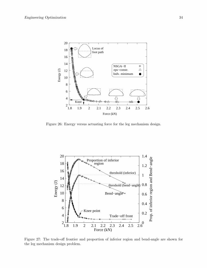
Engineering Optimization 34
foot pathLocus of
Indv. minimum
NSGA−IIeps−constr.
Knee 2
4
6
8
10
12
14
16
18
20
1.8 1.9 2 2.1 2.2 2.3 2.4 2.5 2.6
Ene
rgy
(J)
Force (kN)
Figure 26: Energy versus actuating force for the leg mechanism design.
Trade−off front
regionProportion of inferior
Bend−angle
threshold (inferior)
threshold (bend−angle)
Knee point
2
18
20
1.8 1.9 2 2.1 2.2 2.3 2.4 2.5 2.6 0
0.2
0.4
0.6
0.8
1
1.2
1.4
Ene
rgy
(J)
Force (kN)
14
12
10
8
6
4
16
Pro
p. o
f inf
erio
r re
gion
and
Ben
d−an
gle
Figure 27: The trade-off frontier and proportion of inferior region and bend-angle are shown forthe leg mechanism design problem.
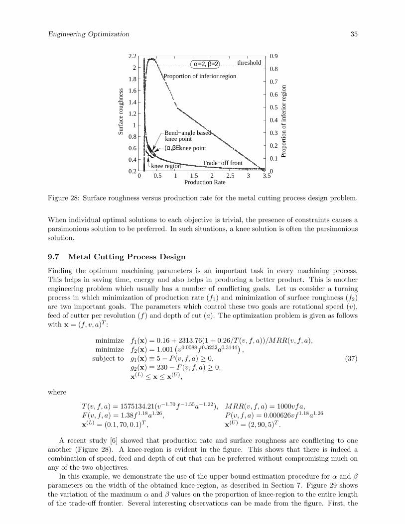
Engineering Optimization 35
threshold
knee region{
Bend−angle basedknee point
knee point(α,β)−
α=2, β=2
1.8
2
2.2
0 0.5 1 1.5 2 2.5 3 3.5 0
0.1
0.2
0.3
0.4
0.5
0.6
0.7
0.8
0.9
Sur
face
rou
ghne
ss
Pro
port
ion
of in
ferio
r re
gion
1.4
1.2
1
0.8
Trade−off front
0.6
0.4
0.2
1.6
Proportion of inferior region
Production Rate
Figure 28: Surface roughness versus production rate for the metal cutting process design problem.
When individual optimal solutions to each objective is trivial, the presence of constraints causes aparsimonious solution to be preferred. In such situations, a knee solution is often the parsimonioussolution.
9.7 Metal Cutting Process Design
Finding the optimum machining parameters is an important task in every machining process.This helps in saving time, energy and also helps in producing a better product. This is anotherengineering problem which usually has a number of conflicting goals. Let us consider a turningprocess in which minimization of production rate (f1) and minimization of surface roughness (f2)are two important goals. The parameters which control these two goals are rotational speed (v),feed of cutter per revolution (f) and depth of cut (a). The optimization problem is given as followswith x = (f, v, a)T :
minimize f1(x) = 0.16 + 2313.76(1 + 0.26/T (v, f, a))/MRR(v, f, a),minimize f2(x) = 1.001
(
v0.0088f0.3232a0.3144)
,subject to g1(x) ≡ 5 − P (v, f, a) ≥ 0,
g2(x) ≡ 230 − F (v, f, a) ≥ 0,
x(L) ≤ x ≤ x(U),
(37)
where
T (v, f, a) = 1575134.21(v−1.70f−1.55a−1.22), MRR(v, f, a) = 1000vfa,F (v, f, a) = 1.38f1.18a1.26, P (v, f, a) = 0.000626vf1.18a1.26
x(L) = (0.1, 70, 0.1)T , x(U) = (2, 90, 5)T .
A recent study [6] showed that production rate and surface roughness are conflicting to oneanother (Figure 28). A knee-region is evident in the figure. This shows that there is indeed acombination of speed, feed and depth of cut that can be preferred without compromising much onany of the two objectives.
In this example, we demonstrate the use of the upper bound estimation procedure for α and βparameters on the width of the obtained knee-region, as described in Section 7. Figure 29 showsthe variation of the maximum α and β values on the proportion of knee-region to the entire lengthof the trade-off frontier. Several interesting observations can be made from the figure. First, the
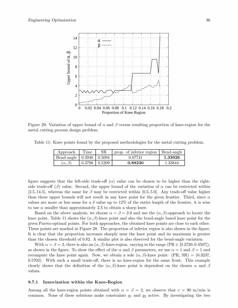
Engineering Optimization 36
Upp
er b
ound
of
0.2Proportion of Knee Region
αβ
0
2
4
6
8
10
12
14
0 0.02 0.04 0.06 0.08 0.1 0.12 0.14 0.16 0.18
α, β
Figure 29: Variation of upper bound of α and β versus resulting proportion of knee-region for themetal cutting process design problem.
Table 11: Knee points found by the proposed methodologies for the metal cutting problem.
Approach Time SR prop. of inferior region Bend-angle
Bend-angle 0.3946 0.5094 0.87741 1.33926
(α, β) 0.3796 0.5209 0.88230 1.33844
figure suggests that the left-side trade-off (α) value can be chosen to be higher than the right-side trade-off (β) value. Second, the upper bound of the variation of α can be restricted within[2.5, 14.5], whereas the same for β may be restricted within [0.5, 5.0]. Any trade-off value higherthan these upper bounds will not result in any knee point for the given frontier. Third, since αvalues are more or less same for a δ value up to 12% of the entire length of the frontier, it is wiseto use α smaller than approximately 2.5 to obtain a sharp knee.
Based on the above analysis, we choose α = β = 2.0 and use the (α, β)-approach to locate theknee point. Table 11 shows the (α, β)-knee point and also the bend-angle based knee point for thegiven Pareto-optimal points. For both approaches, the obtained knee points are close to each other.These points are marked in Figure 28. The proportion of inferior region is also shown in the figure.It is clear that the proportion increases sharply near the knee point and its maximum is greaterthan the chosen threshold of 0.82. A similar plot is also observed for the bend-angle variation.
With α = β = 2, there is also an (α, β)-knee-region, varying in the range (PR ∈ [0.2720, 0.4507]),as shown in the figure. To show the effect of the α and β parameters, we use α = 1 and β = 1 andrecompute the knee point again. Now, we obtain a sole (α, β)-knee point: (PR, SR) = (0.3237,0.5702). With such a small trade-off, there is no knee-region for the same front. This exampleclearly shows that the definition of the (α, β)-knee point is dependent on the chosen α and βvalues.
9.7.1 Innovization within the Knee-Region
Among all the knee-region points obtained with α = β = 2, we observe that v = 90 m/min iscommon. None of these solutions make constraints g1 and g2 active. By investigating the two
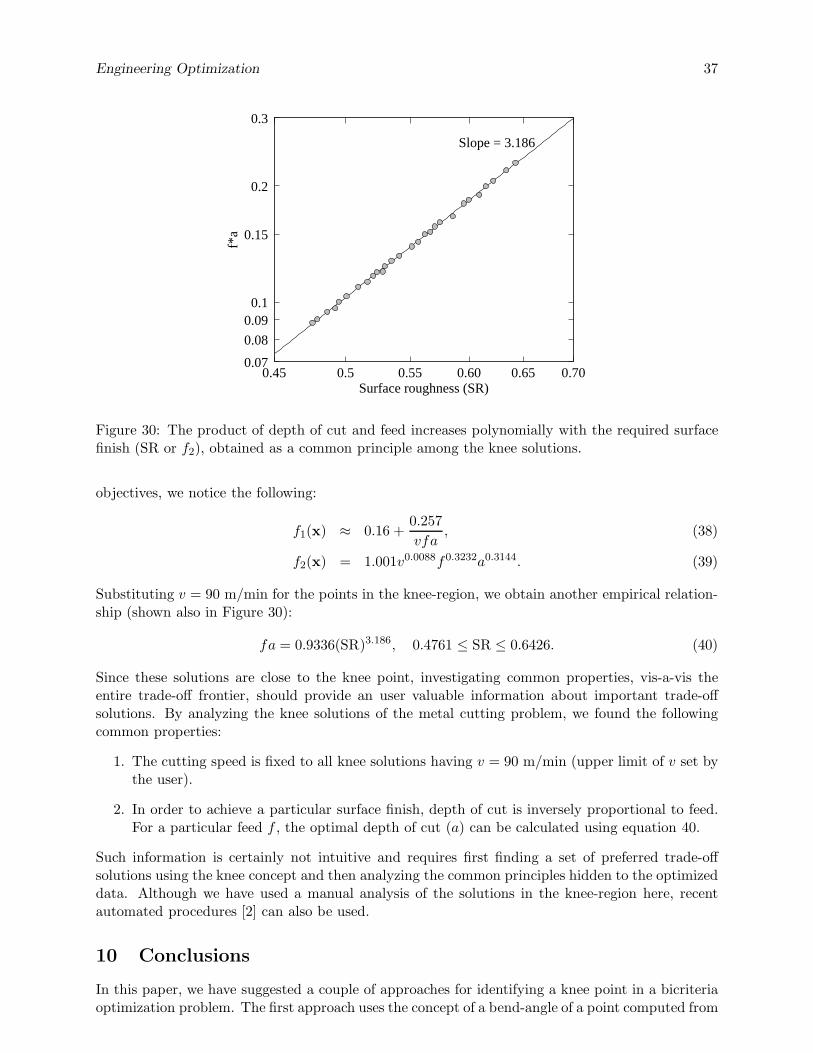
Engineering Optimization 37
Slope = 3.186
0.2
0.15
0.10.09
0.08
0.070.700.650.600.550.50.45
f*a
Surface roughness (SR)
0.3
Figure 30: The product of depth of cut and feed increases polynomially with the required surfacefinish (SR or f2), obtained as a common principle among the knee solutions.
objectives, we notice the following:
f1(x) ≈ 0.16 +0.257
vfa, (38)
f2(x) = 1.001v0.0088f0.3232a0.3144. (39)
Substituting v = 90 m/min for the points in the knee-region, we obtain another empirical relation-ship (shown also in Figure 30):
fa = 0.9336(SR)3.186, 0.4761 ≤ SR ≤ 0.6426. (40)
Since these solutions are close to the knee point, investigating common properties, vis-a-vis theentire trade-off frontier, should provide an user valuable information about important trade-offsolutions. By analyzing the knee solutions of the metal cutting problem, we found the followingcommon properties:
1. The cutting speed is fixed to all knee solutions having v = 90 m/min (upper limit of v set bythe user).
2. In order to achieve a particular surface finish, depth of cut is inversely proportional to feed.For a particular feed f , the optimal depth of cut (a) can be calculated using equation 40.
Such information is certainly not intuitive and requires first finding a set of preferred trade-offsolutions using the knee concept and then analyzing the common principles hidden to the optimizeddata. Although we have used a manual analysis of the solutions in the knee-region here, recentautomated procedures [2] can also be used.
10 Conclusions
In this paper, we have suggested a couple of approaches for identifying a knee point in a bicriteriaoptimization problem. The first approach uses the concept of a bend-angle of a point computed from
Engineering Optimization 38
two extreme points and identifies the point with the maximum bend-angle as the knee point. On theother hand, the second approach uses the supplied critical trade-off information to identify the pointwhich maximizes the region that is inferior to the point based on the trade-off information. Basedon the cone-dominated approach, we have also proposed the idea of a knee-region for problems inwhich instead of a single solution, a set of consecutive solutions may qualify as knee-like solutions.Similarly, instead of the knee point lying in the intermediate region of the trade-off frontier, aknee point may also exist near one of the extreme solutions. We have proposed the concept of anedge-knee point for this purpose. The ideas proposed for identifying a knee point, a knee regionand an edge-knee point have been illustrated well on a tunable test problem exhibiting a knee withvarying sharpness.
We have also reviewed the various approaches that have been employed by researchers to defineor find knee related points. Most of these techniques fall short in completely elaborating the conceptof knee but with the ideas propagated through this paper, efforts can be made to fill the gaps inthese definitions as well. This paper has made a comprehensive discussion of knee and relatedpreferred points and suggested procedures for identifying them.
Furthermore, to facilitate an user to choose appropriate trade-off parameter values, we havesuggested an upper bound estimation procedure from the given trade-off frontier. This analysisprovides a sensitivity of the upper bounds of trade-off parameters on the width of the resultingknee-region. Such an analysis should help researchers and applicationists to get a priori informationabout the range of trade-off parameters which may provide a knee or a knee-like point on a giventrade-off frontier.
There is no denying the fact that knee solutions, if exist, are the most important solutions toa decision maker but the fact that not all bicriteria problems have a knee or a knee-like solutionsuggests that there could be some special relationship between problem parameters and objectivesthat may result in a trade-off front exhibiting a knee. Using the first and second-order gradients ofthe trade-off frontier, we have revealed certain properties which will cause the frontier to exhibita knee. Such properties are important and can be used to design test problems having knees andshould help advance the understanding and discovery of knee points better.
Since the knee points are usually preferred solutions, we have argued that the reason for theexistence of a popular preferred solution methodology in certain problem-solving tasks is relatedto it being a knee point in a underlying bicriteria problem. We have chosen a number of genericproblem-solving tasks, such as sorting, regression, clustering and a few engineering design problemsto illustrate this aspect. The relation between knee points in a bicriteria problem and popularityof certain solution methodologies is interesting and should help develop efficient solution method-ologies in other problem-solving tasks.
Acknowledgments
The study is funded by Department of Science and Technology, Government of India under SERC-Engineering Sciences scheme (No. SR/S3/MERC/091/2009).
References
[1] H. K. Al-Omishy. Prediction of the fuel consumption of petrol and diesel vehicles from acomputer simulation model. Energy, 14(9):563–570, 1989.
[2] S. Bandaru and K. Deb. Automated discovery of vital knowledge from pareto-optimal solu-tions: First results from engineering design. In World Congress on Computational Intelligence(WCCI-2010). IEEE Press, 2010.
Engineering Optimization 39
[3] S. Bechikh, L. Ben Said, and K. Ghedira. Searching for knee regions in multi-objective op-timization using mobile reference points. In Proceedings of the 2010 ACM Symposium onApplied Computing, pages 1118–1125. ACM, 2010.
[4] J. Branke, K. Deb, H. Dierolf, and M. Osswald. Finding knees in multi-objective optimization.In Parallel Problem Solving from Nature (PPSN-VIII), pages 722–731. Heidelberg, Germany:Springer, 2004. LNCS 3242.
[5] I. Das. On characterizing the “knee” of the Pareto curve based on normal-boundary intersec-tion. Structural Optimization, 18:107–115, 1999.
[6] R. Datta and K. Deb. A classical-cum-evolutionary multi-objective optimization for optimalmachining parameters. In World Congress on Nature and Biologically Inspired Computing(NaBIC-2009), pages 607–612, 2009.
[7] K. Deb. Multi-objective optimization using evolutionary algorithms. Wiley, Chichester, UK,2001.
[8] K. Deb, J. Sundar, N. Uday, and S. Chaudhuri. Reference point based multi-objective opti-mization using evolutionary algorithms. International Journal of Computational IntelligenceResearch (IJCIR), 2(6):273–286, 2006.
[9] K. Deb and S. Tiwari. Multi-objective optimization of a leg mechanism using genetic algo-rithms. Engineering Optimization, 37(4):325–350, 2005.
[10] F. Dion, H. Rakha, and Y. S. Kang. Comparison of delay estimates at under-saturated andover-saturated pre-timed signalized intersections. Transportation Research Part B, 38:99–122,2004.
[11] L. Fu and B. Hellinga. Delay variability at signalized intersections. Transportation ResearchRecord: Journal of the Transportation Research Board, (1710):215–221, 2000.
[12] D. B. Kamerud. The 55 mph speed limit: Costs, benefits, and implied trade-offs. Technicalreport, Societal Analysis Department, General Motors Research Laboratories,, Warren, U.S.A.,1981.
[13] C. A. Mattson, A. A. Muller, and A. Messac. Smart pareto filter: Obtaining a minimalrepresentation of multiobjective design space. Engineering Optimization, 36(6):721–740, 2004.
[14] K. Miettinen. Nonlinear Multiobjective Optimization. Kluwer, Boston, 1999.
[15] L. Rachmawati and D. Srinivasan. A multiobjective evolutionary algorithm with weighted-sumniching for convergence on knee regions. In Proceedings of IEEE Congress on EvolutionaryComputation (CEC-2006), pages 1916–1923, 2006.
[16] L. Rachmawati and D. Srinivasan. Multiobjective evolutionary algorithm with controllablefocus on the knees of the pareto front. IEEE Transactions on Evolutionary Computation,13(4):810–824, 2009.
[17] D. Ruppert, M. P. Wand, and R. J. Carroll. Semiparametric regression. Cambridge UniversityPress, 2003.
[18] O. Schutze, M. Laumanns, and C. A. Coello Coello. Approximating the knee of an mopwith stochastic search algorithm. In Parallel Problem Solving from Nature (PPSN X), (LNCS5199), pages 795–804. Heidelberg, Berlin: Springer, 2008.