Embed Size (px)
Citation preview
Discussion Papers
Statistics NorwayResearch department
No. 696 •June 2012
Petter Osmundsen, Knut Einar Rosendahl and Terje Skjerpen
Understanding rig rates

Discussion Papers No. 696, June 2012 Statistics Norway, Research Department
Petter Osmundsen, Knut Einar Rosendahl and Terje Skjerpen
Understanding rig rates
Abstract: We examine the largest cost component in offshore development projects, drilling rates, which have been high in recent years. To our knowledge, rig rates have not been analysed empirically before in the economic literature. Using econometric analysis, we examine the effects of gas and oil prices, rig capacity utilisation, contract length and lead time, and rig-specific characteristics on Gulf of Mexico rig rates. Having access to a unique data set containing contract information, we are able to estimate how contract parameters crucial to the relative bargaining power between rig owners and oil and gas companies affects rig rates. Our econometric framework is a single equation random effects model, in which the systematic part of the equation is non-linear in the parameters. Such a model belongs to the class of non-linear mixed models, which has been heavily utilised in the biological sciences.
Keywords: Rig contracts; GoM rig rates; Panel data
JEL classification: C18; C23; L14; L71; Q4
Acknowledgements: Thanks are due to Sven Ziegler, a number of specialists in oil and rig companies and Torbjørn Hægeland for useful suggestions and comments. We thank RS Platou for data and the Research Council of Norway for funding.
Address: Petter Osmundsen, University of Stavanger, NO-4036 Stavanger, Norway. E-mail: [email protected]
Knut Einar Rosendahl, Statistics Norway, Research Department. E-mail: [email protected]
Terje Skjerpen, Statistics Norway, Research Department. E-mail: [email protected]
Discussion Papers comprise research papers intended for international journals or books. A preprint of a Discussion Paper may be longer and more elaborate than a standard journal article, as it may include intermediate calculations and background material etc.
© Statistics Norway Abstracts with downloadable Discussion Papers in PDF are available on the Internet: http://www.ssb.no http://ideas.repec.org/s/ssb/dispap.html For printed Discussion Papers contact: Statistics Norway Telephone: +47 62 88 55 00 E-mail: [email protected] ISSN 0809-733X Print: Statistics Norway
3
Sammendrag
Borekostnader er den viktigste kostnadskomponenten i olje- og gassproduksjon til havs. Leie av
borerigger har vært spesielt dyrt de siste årene. Ved bruk av økonometriske analyser studerer vi hva
som påvirker riggratene i Mexico-golfen, det vil si kostnadene per døgn for å leie en borerigg. Viktige
faktorer er gass- og oljepriser, kapasitetsutnytting for borerigger, kontraktslengde og -ledetid, og rigg-
spesifikke faktorer. Vi har fått tilgang til et unikt datasett med kontraktsinformasjon som gjør det
mulig å teste hvordan kontraktsmessige forhold påvirker riggratene. Slike kontraktsmessige forhold er
viktige i spillet mellom riggeiere og olje- og gasselskaper. Vårt økonometriske rammeverk er basert på
en ikke-lineær paneldatamodell med tilfeldige riggspesifikke effekter. Ikke-lineæriteten i den
systematiske delen av relasjonen skyldes at gass- og oljepris inngår som forklaringsvariabler i
modellen via et CES-prisaggregat. Modeller av denne typen er et medlem i klassen av ikke-lineære
blandede modeller, som brukes intensivt innenfor biologisk forskning.
4
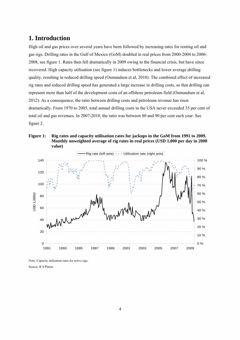
1. Introduction High oil and gas prices over several years have been followed by increasing rates for renting oil and
gas rigs. Drilling rates in the Gulf of Mexico (GoM) doubled in real prices from 2000-2004 to 2006-
2008, see figure 1. Rates then fell dramatically in 2009 owing to the financial crisis, but have since
recovered. High capacity utilisation (see figure 1) induces bottlenecks and lower average drilling
quality, resulting in reduced drilling speed (Osmundsen et al, 2010). The combined effect of increased
rig rates and reduced drilling speed has generated a large increase in drilling costs, so that drilling can
represent more than half of the development costs of an offshore petroleum field (Osmundsen et al,
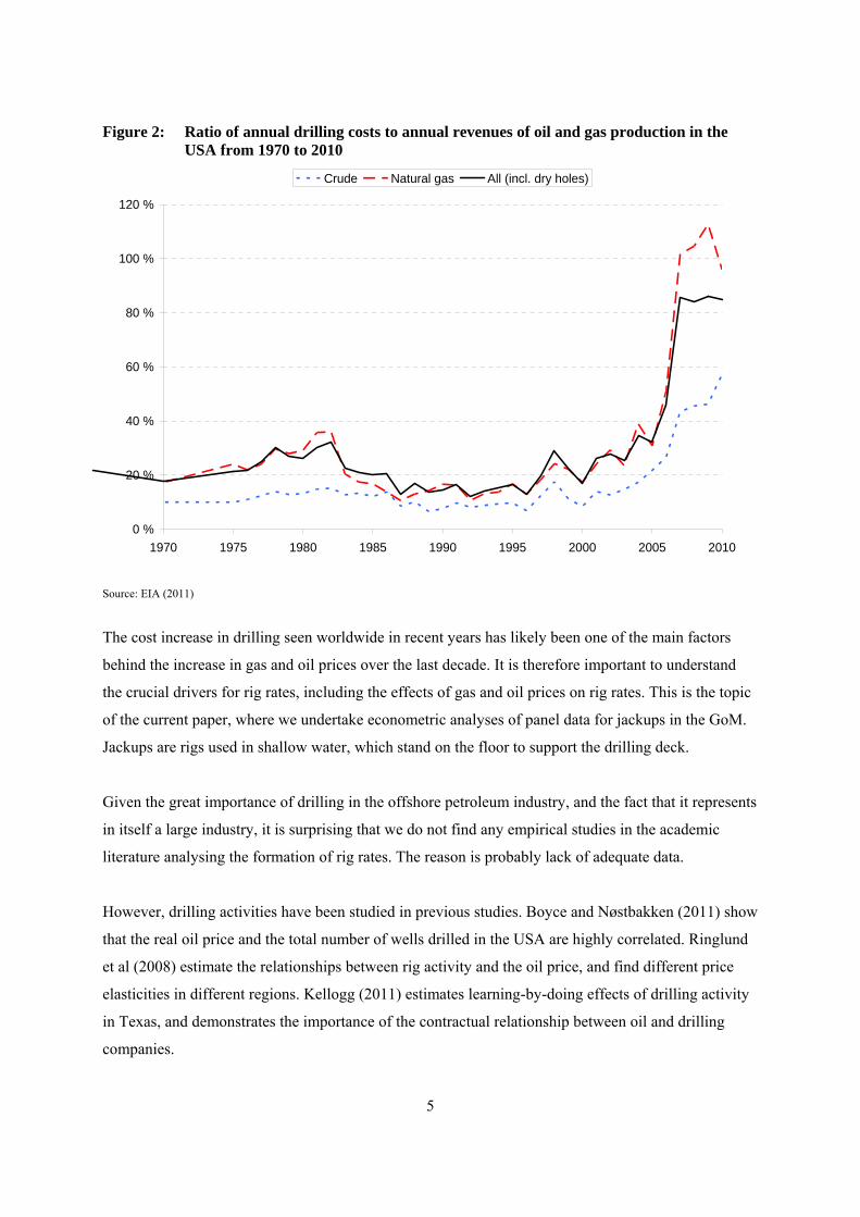
2012). As a consequence, the ratio between drilling costs and petroleum revenue has risen
dramatically. From 1970 to 2005, total annual drilling costs in the USA never exceeded 35 per cent of
total oil and gas revenues. In 2007-2010, the ratio was between 80 and 90 per cent each year. See
figure 2.
Figure 1: Rig rates and capacity utilisation rates for jackups in the GoM from 1991 to 2009. Monthly unweighted average of rig rates in real prices (USD 1,000 per day in 2008 value)
0
20
40
60
80
100
120
140
1991 1993 1995 1997 1999 2001 2003 2005 2007 2009
US
D 1
,000
/d
0 %
10 %
20 %
30 %
40 %
50 %
60 %
70 %
80 %
90 %
100 %
Rig rate (left axis) Utilization rate (right axis)
Note: Capacity utilisation rates for active rigs.
Source: R S Platou
5
Figure 2: Ratio of annual drilling costs to annual revenues of oil and gas production in the USA from 1970 to 2010
0 %
20 %
40 %
60 %
80 %
100 %
120 %
1970 1975 1980 1985 1990 1995 2000 2005 2010
Crude Natural gas All (incl. dry holes)
Source: EIA (2011)
The cost increase in drilling seen worldwide in recent years has likely been one of the main factors
behind the increase in gas and oil prices over the last decade. It is therefore important to understand
the crucial drivers for rig rates, including the effects of gas and oil prices on rig rates. This is the topic
of the current paper, where we undertake econometric analyses of panel data for jackups in the GoM.
Jackups are rigs used in shallow water, which stand on the floor to support the drilling deck.
Given the great importance of drilling in the offshore petroleum industry, and the fact that it represents
in itself a large industry, it is surprising that we do not find any empirical studies in the academic
literature analysing the formation of rig rates. The reason is probably lack of adequate data.
However, drilling activities have been studied in previous studies. Boyce and Nøstbakken (2011) show
that the real oil price and the total number of wells drilled in the USA are highly correlated. Ringlund
et al (2008) estimate the relationships between rig activity and the oil price, and find different price
elasticities in different regions. Kellogg (2011) estimates learning-by-doing effects of drilling activity
in Texas, and demonstrates the importance of the contractual relationship between oil and drilling
companies.
6
In our paper, we analyse a unique dataset from international offshore broker R S Platou that contains
contract information and technical data for the rigs in the GoM, in particular rig rates, contract length
and lead time. The GoM is a reasonably well defined submarket for jackups owing to moving costs
and the difficulties of restaffing (Corts, 2008).
When oil and gas companies contract for drilling rigs, they primarily use short-term well-to-well
contracts awarded through a bidding process among the owners of suitable nearby rigs (Corts, 2008).
Most of the GoM rig contracts have remuneration in the form of day rates (Corts, 2000; Corts and
Singh, 2004). Even though producers do not physically drill their own wells, they do design wells and
write drilling procedures, since producers typically have more geological information than drilling
companies (Kellogg, 2011).
Rig rates are volatile, following a clear cyclical pattern. Not surprisingly, rig rates are highly sensitive
to gas and oil prices and to capacity utilisation. We also examine the effect of contract length and lead
time, build year, drilling depth capacity and rig classification. Rig rate formation is interesting in terms
of the bargaining situation between rig owners and oil companies. With our access to contract data, we
are able to test the effect of contract features such as contract length and lead time on pricing in a
contract market. In a series of meetings with oil companies, rig companies and rig analysts, we have
gained insight into the bargaining situation for rig rates. The relative bargaining power of rig owners
and oil companies is likely to have an impact on the level of rig rates. Thus, factors that affect the
relative bargaining power of the contracting parties form our ex ante hypotheses on rig rate formation.
Obviously, high current capacity utilisation in the rig industry is crucial to the bargaining power of the
rig companies, and is – ceteris paribus – likely to lead to high rig rates. The same applies to high
expected gas and oil prices, which make more development projects profitable and hence stimulate rig
demand. However, jackup rigs are rented in a contract market, so that contract length and lead times
also play a significant role. In periods of high demand, rig owners can demand longer contracts and,
together with increased lead times, that reflects a strong future market. This enhances the bargaining
power of the rig companies and leads to an increase in rig rates for new contracts.
In our econometric framework, we consider a random effects model where the parameters enter non-
linearly in the systematic part of the equation. The non-linearity arises from representing the effects of
gas and oil prices through a CES price aggregate. Our model can be considered a member of the
nonlinear mixed effects type in the statistical literature (see eg, Vonesh and Chinchilli, 1997;
7
Davidian, 2009 and Serroyen et al, 2009). Such models have been heavily utilised in the biological
sciences, but have, to our knowledge, not been utilised previously for economic applications.
Our findings are specific results pertaining to the GoM jackup market, but the main conclusions are of
a more general nature. As for the latter, the unique data set contains detailed contract information – in
particular lead times and contract length – which generates results on how contract structure affects
pricing. The hypotheses of our industry panel are confirmed. Not only gas and oil prices and capacity
utilisation, but also contract length and lead time positively affect rig rates. High capacity utilisation
occurs in periods with high gas and oil prices, ie, higher gas and oil prices may not only have a direct
effect on rig rates, but also an indirect effect by increasing the utilisation rate. Rig rates only partly
respond to a sudden shift in gas and oil prices – oil and gas companies wait for some months to see if
the price change is more permanent before they increase rig demand. Gas prices are much more
important than oil prices for changes in rig rates, which is consistent with the fact that jackups in the
GoM area are used mostly for gas drilling. As for market specifics, we find that rig rates are almost
proportional to the technical depth capacity of the rig.
The remainder of the paper is organised as follows. Section 2 outlines the theoretical background for
our empirical analysis. The econometric approach is developed in section 3. Section 4 describes our
data, and empirical results are presented in section 5. Section 6 concludes.
2. Theoretical background In this section, we will motivate the empirical model by using a simple analytical framework which
includes the most important variables in our model.
2.1 Oil and gas companies’ demand for rigs
Oil and gas companies use rigs to explore for oil and gas, and to develop oil and gas fields. They
typically have a number of projects with different expected profitability, and the expected value of
each project is increasing in the expected prices of gas (pG) and/or oil (pO). For some projects, eg,
developing a gas or oil field, only one of these prices may be of importance, whereas for other projects
– such as exploration for or development of an oil field with associated gas – both prices may be
important. Let π denote the price of renting a rig (rig rate). The net benefits from using r rigs within a
time period may then be expressed as B(pG,pO,r) – πr, with , 0G Op pB B > , Br > 0 and Brr < 0 (Bx and Bxy
8
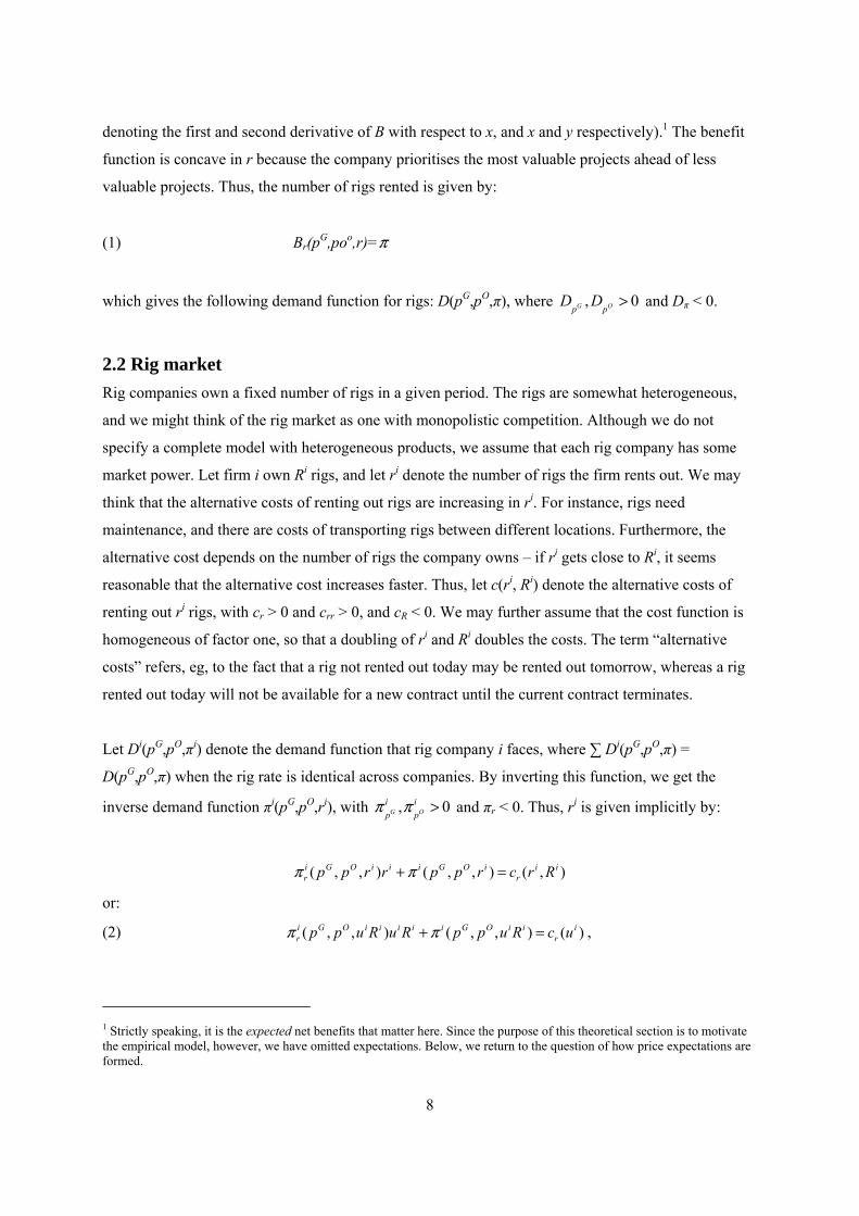
denoting the first and second derivative of B with respect to x, and x and y respectively).1 The benefit
function is concave in r because the company prioritises the most valuable projects ahead of less
valuable projects. Thus, the number of rigs rented is given by:
(1) Br(pG,poo,r)=π
which gives the following demand function for rigs: D(pG,pO,π), where , 0G Op pD D > and Dπ < 0.
2.2 Rig market
Rig companies own a fixed number of rigs in a given period. The rigs are somewhat heterogeneous,
and we might think of the rig market as one with monopolistic competition. Although we do not
specify a complete model with heterogeneous products, we assume that each rig company has some
market power. Let firm i own Ri rigs, and let ri denote the number of rigs the firm rents out. We may
think that the alternative costs of renting out rigs are increasing in ri. For instance, rigs need
maintenance, and there are costs of transporting rigs between different locations. Furthermore, the
alternative cost depends on the number of rigs the company owns – if ri gets close to Ri, it seems
reasonable that the alternative cost increases faster. Thus, let c(ri, Ri) denote the alternative costs of
renting out ri rigs, with cr > 0 and crr > 0, and cR < 0. We may further assume that the cost function is
homogeneous of factor one, so that a doubling of ri and Ri doubles the costs. The term “alternative
costs” refers, eg, to the fact that a rig not rented out today may be rented out tomorrow, whereas a rig
rented out today will not be available for a new contract until the current contract terminates.
Let Di(pG,pO,πi) denote the demand function that rig company i faces, where ∑ Di(pG,pO,π) =
D(pG,pO,π) when the rig rate is identical across companies. By inverting this function, we get the
inverse demand function πi(pG,pO,ri), with , 0G O
i i
p pπ π > and πr < 0. Thus, ri is given implicitly by:
( , , ) ( , , ) ( , )i G O i i i G O i i ir rp p r r p p r c r Rπ π+ =
or:
(2) ( , , ) ( , , ) ( )i G O i i i i i G O i i ir rp p u R u R p p u R c uπ π+ = ,
1 Strictly speaking, it is the expected net benefits that matter here. Since the purpose of this theoretical section is to motivate the empirical model, however, we have omitted expectations. Below, we return to the question of how price expectations are formed.
9
where u = ri/Ri denotes the utilisation rate of company i. The last equation then follows from the
homogeneity assumption. With normal demand functions D, we then have that both ri (or ui) and πi
increase in pG and pO.
What about u, the aggregate utilisation rate in the rig market? It seems reasonable to argue that the
degree of competition in the market depends on the number of available rigs. That is, if the utilisation
rate is high, each rig company will acquire more market power as the inverse demand function it faces
becomes steeper (fewer available substitutes, ie, rigs). Assuming that the utilisation rate in period t+1
is correlated with the utilisation rate in period t, it also seems reasonable to assume that the alternative
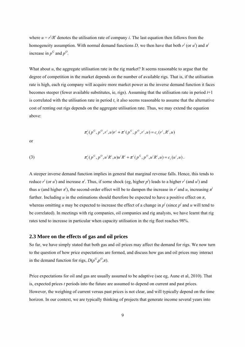
cost of renting out rigs depends on the aggregate utilisation rate. Thus, we may extend the equation
above:
( , , , ) ( , , , ) ( , , )i G O i i i G O i i ir rp p r u r p p r u c r R uπ π+ =
or
(3) ( , , , ) ( , , , ) ( , )i G O i i i i i G O i i ir rp p u R u u R p p u R u c u uπ π+ = .
A steeper inverse demand function implies in general that marginal revenue falls. Hence, this tends to
reduce ri (or ui) and increase πi. Thus, if some shock (eg, higher pj) leads to a higher ri (and ui) and
thus u (and higher πi), the second-order effect will be to dampen the increase in ri and u, increasing πi
further. Including u in the estimations should therefore be expected to have a positive effect on π,
whereas omitting u may be expected to increase the effect of a change in pj (since pj and u will tend to
be correlated). In meetings with rig companies, oil companies and rig analysts, we have learnt that rig
rates tend to increase in particular when capacity utilisation in the rig fleet reaches 98%.
2.3 More on the effects of gas and oil prices
So far, we have simply stated that both gas and oil prices may affect the demand for rigs. We now turn
to the question of how price expectations are formed, and discuss how gas and oil prices may interact
in the demand function for rigs, D(pG,pO,π).
Price expectations for oil and gas are usually assumed to be adaptive (see eg, Aune et al, 2010). That
is, expected prices t periods into the future are assumed to depend on current and past prices.
However, the weighing of current versus past prices is not clear, and will typically depend on the time
horizon. In our context, we are typically thinking of projects that generate income several years into
10
the future, but there are significant differences between the time horizons for exploratory drilling and
got drilling additional wells in a developed field. We will use price indices for gas and oil that are
weighted sums of the current prices and the price indices in the previous period, and leave it up to the
estimations to determine the relative weights. The price indices, which we will refer to as smoothed
prices, are specified in the next section.
Although some companies specialise in either oil or gas extraction, most companies in this industry
are involved in both types of extraction. Many petroleum fields contain both gas and oil, and the actual
content is often not revealed before test drilling has been undertaken. Oil and gas reserves are usually
imperfect substitutes to the companies, because they require different types of skills and capacity. In
particular, gas is more challenging in terms of transport. A common way of modelling imperfect
substitutes is to use a constant elasticity of substitution (CES) function. Thus, we will consider a CES
aggregate of gas and oil reserves, and let the estimation determine both the elasticity of substitution
and the relative importance of the two resources. A large elasticity means that gas and oil are almost
perfect substitutes and, in the limiting case where elasticity verges on infinity, the benefits of gas and
oil are fully separable.
Given the CES structure, we can furthermore construct a price index for the CES aggregate. See the
next section. Above, we argued that the rig rate increases in line with gas and oil prices. In the
empirical model below, we will specify a log-linear function of the CES price aggregate (of smoothed
gas and oil prices).
2.4 Other variables
The modelling above treats all rigs as identical, but assumes at the same time that they are
heterogeneous. We have some information about heterogeneous characteristics of the rigs, such as rig
category and technical depth capacity. These are assumed to affect the contract rates, and are treated as
dummy (eg, rig categories) or ordinary variables (eg, technical depth). The contract structure is vital to
rig rate determination. Our unique data set contains detailed contract information, in particular lead
times and contract length.
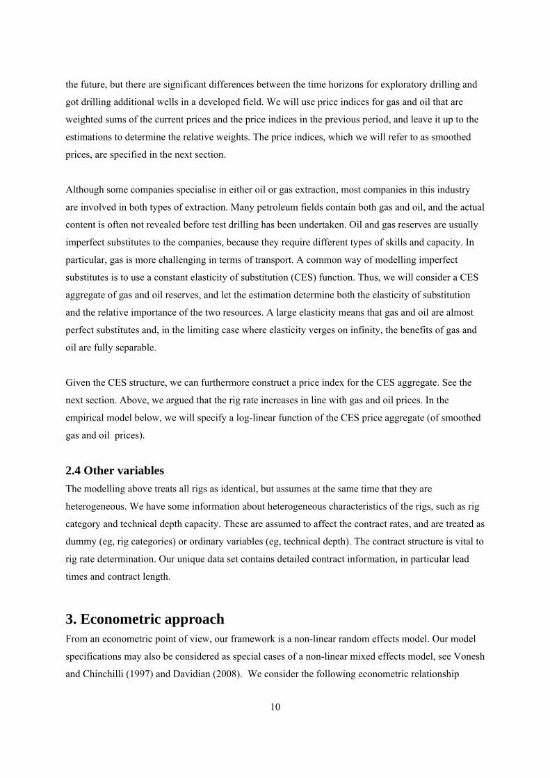
3. Econometric approach From an econometric point of view, our framework is a non-linear random effects model. Our model
specifications may also be considered as special cases of a non-linear mixed effects model, see Vonesh
and Chinchilli (1997) and Davidian (2008). We consider the following econometric relationship
11
(4) 0 1 2
3 4 5 6 7
4 2009
2 1991
log( ) log( ( , , , )) log(1 ) (1 )
log( )
.
is is gas oil is is
is is is i i
m i j is i ism j
RIGRATE PCES UTIL HIGHUTIL
HIGHUTIL LEAD CONT BUILD DEPTH
DUMCATm DUMj
β β α α δ σ ββ β β β β
γ λ μ ε= =
= + × + × − × −
+ × + × + × + × + +
× + × + +
The individual rigs have the status of observational units. They are denoted by subscripts i (rig
number), whereas subscript s denotes the observation number.2 Most of the variables in (4) are both
rig- and contract-specific, and thus have both subscripts. This also includes the CES price aggregate,
since s denotes the observation number and not time. If the observation number s for two rigs is from
the same period, however, the variable will take the same value for both observational units.
PCESis(αgas,αoil,δ,σ) denotes the CES aggregate of smoothed real gas and oil prices on index form (see
below), where αgas and αoil denote smoothing parameters for gas and oil prices respectively, δ is a
distribution parameter and σ the substitution elasticity. The price index PCESis is calculated for the
time period (month) when the contract is signed.
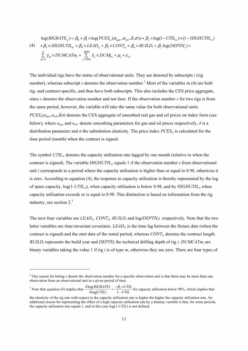
The symbol UTILis denotes the capacity utilisation rate lagged by one month (relative to when the
contract is signed). The variable HIGHUTILis equals 1 if the observation number s from observational
unit i corresponds to a period where the capacity utilisation is higher than or equal to 0.98, otherwise it
is zero. According to equation (4), the response to capacity utilisation is thereby represented by the log
of spare capacity, log(1-UTILis), when capacity utilisation is below 0.98, and by HIGHUTILis when
capacity utilisation exceeds or is equal to 0.98. This distinction is based on information from the rig
industry, see section 2.3
The next four variables are LEADis, CONTis, BUILDi and log(DEPTHi) respectively. Note that the two
latter variables are time-invariant covariates. LEADis is the time lag between the fixture date (when the
contract is signed) and the start date of the rental period, whereas CONTis denotes the contract length.
BUILDi represents the build year and DEPTHi the technical drilling depth of rig i. DUMCATmi are
binary variables taking the value 1 if rig i is of type m, otherwise they are zero. There are four types of
2 One reason for letting s denote the observation number for a specific observation unit is that there may be more than one observation from an observational unit in a given period of time.
3 Note that equation (4) implies that 2log( )
log( ) 1
RIGRATE UTIL
UTIL UTIL
β∂ − ×=∂ −
for capacity utilisation below 98%, which implies that
the elasticity of the rig rate with respect to the capacity utilisation rate is higher the higher the capacity utilisation rate. An additional reason for representing the effect of a high capacity utilisation rate by a dummy variable is that, for some periods, the capacity utilisation rate equals 1, and in this case log(1-UTIL) is not defined.
12
jackups in our dataset, and rig rates may, ceteris paribus, differ among different rig types.4 The first
type is the reference type, whose level is taken care of by the intercept. We have also added year
dummies. DUMjis is 1 if observation number s from observational unit i occurs in year j (j=1991, …,
2009). The random effect μi for rig i is assumed to be normally distributed, with variance 2μμσ , and εis
denoting a genuine error term. We assume that the genuine errors are normally distributed white noise
errors with a variance given by 2εεσ .
The main reasons for considering a random effects specification are the presence of time-invariant
covariates and the fact that the model is non-linear in the parameters. The effect of time-invariant
variables is not identified in fixed effects models unless further assumptions are introduced.
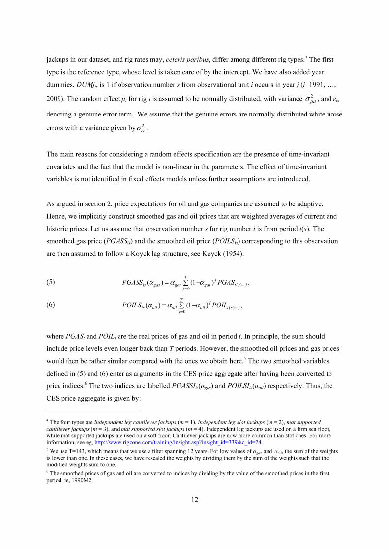
As argued in section 2, price expectations for oil and gas companies are assumed to be adaptive.
Hence, we implicitly construct smoothed gas and oil prices that are weighted averages of current and
historic prices. Let us assume that observation number s for rig number i is from period t(s). The
smoothed gas price (PGASSis) and the smoothed oil price (POILSis) corresponding to this observation
are then assumed to follow a Koyck lag structure, see Koyck (1954):
(5) ( )0
( ) (1 ) .T
jis gas gas gas t s j
jPGASS PGASα α α −
== −
(6) ( )0
( ) (1 ) ,T
jis oil oil oil t s j
jPOILS POILα α α −
== −
where PGASt and POILt are the real prices of gas and oil in period t. In principle, the sum should
include price levels even longer back than T periods. However, the smoothed oil prices and gas prices
would then be rather similar compared with the ones we obtain here.5 The two smoothed variables
defined in (5) and (6) enter as arguments in the CES price aggregate after having been converted to
price indices.6 The two indices are labelled PGASSIis(αgas) and POILSIis(αoil) respectively. Thus, the
CES price aggregate is given by:
4 The four types are independent leg cantilever jackups (m = 1), independent leg slot jackups (m = 2), mat supported cantilever jackups (m = 3), and mat supported slot jackups (m = 4). Independent leg jackups are used on a firm sea floor, while mat supported jackups are used on a soft floor. Cantilever jackups are now more common than slot ones. For more information, see eg, http://www.rigzone.com/training/insight.asp?insight_id=339&c_id=24. 5 We use T=143, which means that we use a filter spanning 12 years. For low values of αgas and αoil, the sum of the weights is lower than one. In these cases, we have rescaled the weights by dividing them by the sum of the weights such that the modified weights sum to one. 6 The smoothed prices of gas and oil are converted to indices by dividing by the value of the smoothed prices in the first period, ie, 1990M2.
13
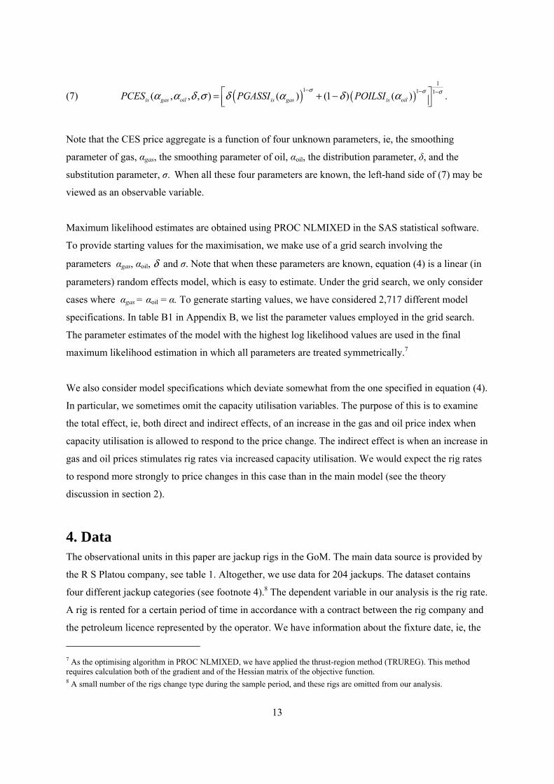
(7) ( ) ( )1
1 1 1( , , , ) ( ) (1 ) ( ) .is gas oil is gas is oilPCES PGASSI POILSIσ σ σα α δ σ δ α δ α
− − − = + −
Note that the CES price aggregate is a function of four unknown parameters, ie, the smoothing
parameter of gas, αgas, the smoothing parameter of oil, αoil, the distribution parameter, δ, and the
substitution parameter, σ. When all these four parameters are known, the left-hand side of (7) may be
viewed as an observable variable.
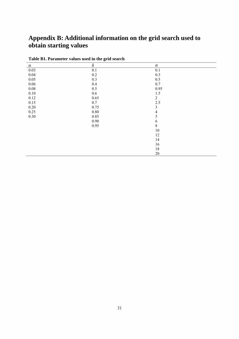
Maximum likelihood estimates are obtained using PROC NLMIXED in the SAS statistical software.
To provide starting values for the maximisation, we make use of a grid search involving the
parameters αgas, αoil, δ and σ. Note that when these parameters are known, equation (4) is a linear (in
parameters) random effects model, which is easy to estimate. Under the grid search, we only consider
cases where αgas = αoil = α. To generate starting values, we have considered 2,717 different model
specifications. In table B1 in Appendix B, we list the parameter values employed in the grid search.
The parameter estimates of the model with the highest log likelihood values are used in the final
maximum likelihood estimation in which all parameters are treated symmetrically.7
We also consider model specifications which deviate somewhat from the one specified in equation (4).
In particular, we sometimes omit the capacity utilisation variables. The purpose of this is to examine
the total effect, ie, both direct and indirect effects, of an increase in the gas and oil price index when
capacity utilisation is allowed to respond to the price change. The indirect effect is when an increase in
gas and oil prices stimulates rig rates via increased capacity utilisation. We would expect the rig rates
to respond more strongly to price changes in this case than in the main model (see the theory
discussion in section 2).
4. Data The observational units in this paper are jackup rigs in the GoM. The main data source is provided by
the R S Platou company, see table 1. Altogether, we use data for 204 jackups. The dataset contains
four different jackup categories (see footnote 4).8 The dependent variable in our analysis is the rig rate.
A rig is rented for a certain period of time in accordance with a contract between the rig company and
the petroleum licence represented by the operator. We have information about the fixture date, ie, the
7 As the optimising algorithm in PROC NLMIXED, we have applied the thrust-region method (TRUREG). This method requires calculation both of the gradient and of the Hessian matrix of the objective function. 8 A small number of the rigs change type during the sample period, and these rigs are omitted from our analysis.
14
date when the contract is signed, as well as the starting and end dates for each contract. From the
amount of money paid for the whole contract period, it is possible to deduce a daily rig rate. The daily
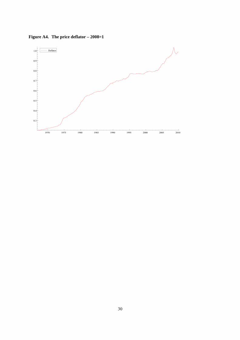
rig rates are in current money and we have deflated them by a producer price index to obtain rig rates
in constant prices.
The data are on a monthly basis, and the timing refers to the point in time when the contract was
signed.9 We possess data for many of the rigs over a substantial period of time, and hence have
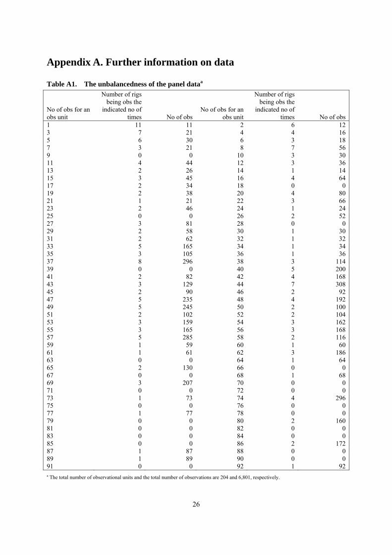
information on different contracts for a specific rig.10 The data set is thus an (unbalanced) panel data
set. In Appendix A, we give an overview of the unbalancedness of the panel data set. The number of
observations for a rig varies from 1 to 92.
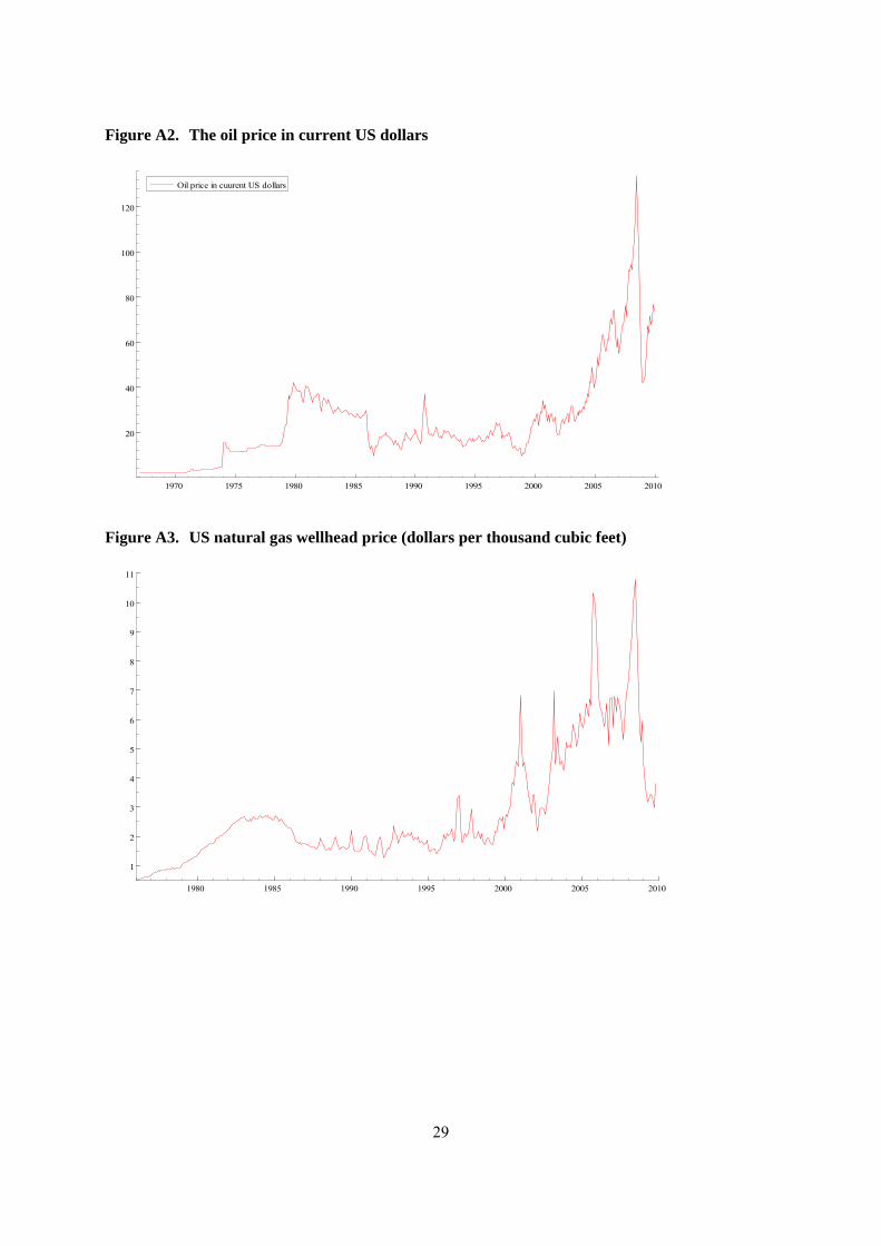
The most important explanatory variables in our estimations are gas and oil prices. For the gas price,
we use US wellhead prices taken from the EIA, whereas for the oil price we use the WTI price. These
prices are deflated by the same price index as rig rates.
The data from RS Platou also provide information on capacity utilisation of jackups in the GoM area.
The data distinguish between capacity utilisation rates for active rigs and for all rigs. Based on
discussions with rig analysts, we use the former in our analysis.11 As the capacity utilisation rate
applies to the whole GoM area, it is equal for all observations from the same time period. From a
theoretical point of view, one may argue that the capacity utilisation rate should not enter linearly in
the model – it seems probable, for example, that rig rates are more sensitive to increases in capacity
utilisation rates when these rates are high (ie, a convex relationship could be expected). This is
captured by our model specification for utilisation rates up to 98% (for higher rates we use a dummy,
as explained above).
A special feature of the panel data used in this analysis is that one may have more than one
observation for a rig at a specific point of time. The reason is the lead time from when the contract is
signed to the period when the rig is involved in a specific drilling project. This delay is represented by
9 As mentioned above, we have information about fixture, start and end date for each contract. However, one problem with the data is that the fixture date is often reported to fall after the start date. The reason is that the reported fixture date is when the contract is officially announced, which is often after the handshake date. We then follow the assumptions applied by R S Platou, which are to set the fixture date 50 days before the start date of the contract whenever the former comes after the latter in the data. 10 Our estimation sample spans the period 1990M2 to 2009M10. 11 Active rigs are defined as rigs that are actively marketed, whereas passive rigs comprise units that are cold stacked for shorter or longer period, in yard, or en route from one body of water to another. For an interesting analysis of decisions by drilling companies to idle (“stack”) rigs in periods with low dayrates, see Corts (2008).
15
an independent variable in our analysis (LEAD). Since the owner of the rig may make different
contracts for the same rig for disjunctive time periods ahead, it follows that one may have more than
one observation for the same rig at a given point of time. As a consequence of this somewhat rare data
design, we find it convenient to use the index s to indicate the observation number for a specific rig.
We will use the index t to indicate calendar time when we need to be explicit about time.
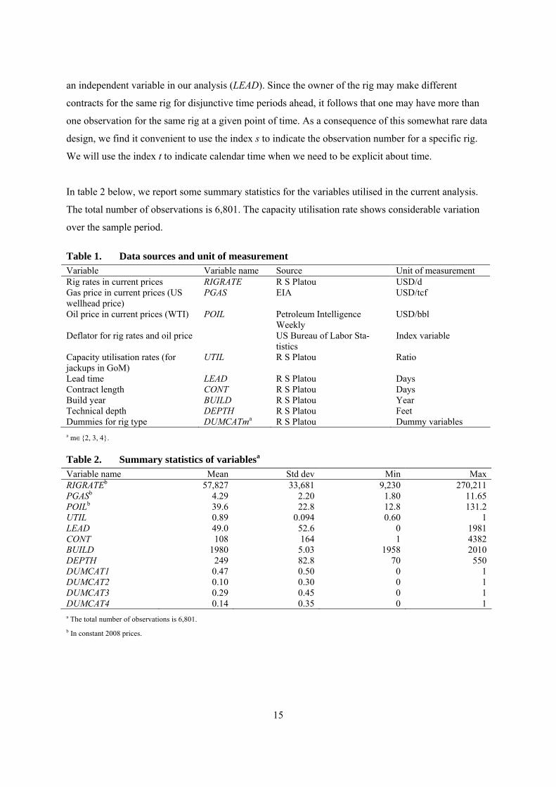
In table 2 below, we report some summary statistics for the variables utilised in the current analysis.
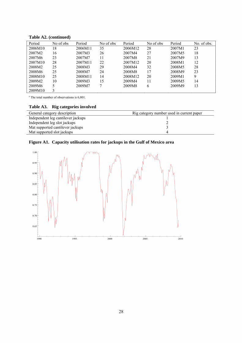
The total number of observations is 6,801. The capacity utilisation rate shows considerable variation
over the sample period.
Table 1. Data sources and unit of measurement Variable Variable name Source Unit of measurement Rig rates in current prices RIGRATE R S Platou USD/d Gas price in current prices (US wellhead price)
PGAS EIA USD/tcf
Oil price in current prices (WTI) POIL Petroleum Intelligence Weekly
USD/bbl
Deflator for rig rates and oil price US Bureau of Labor Sta-tistics
Index variable
Capacity utilisation rates (for jackups in GoM)
UTIL R S Platou Ratio
Lead time LEAD R S Platou Days Contract length CONT R S Platou Days Build year BUILD R S Platou Year Technical depth DEPTH R S Platou Feet Dummies for rig type DUMCATma R S Platou Dummy variables a m∈{2, 3, 4}.
Table 2. Summary statistics of variablesa Variable name Mean Std dev Min Max RIGRATEb 57,827 33,681 9,230 270,211 PGASb 4.29 2.20 1.80 11.65 POILb 39.6 22.8 12.8 131.2 UTIL 0.89 0.094 0.60 1 LEAD 49.0 52.6 0 1981 CONT 108 164 1 4382 BUILD 1980 5.03 1958 2010 DEPTH 249 82.8 70 550 DUMCAT1 0.47 0.50 0 1 DUMCAT2 0.10 0.30 0 1 DUMCAT3 0.29 0.45 0 1 DUMCAT4 0.14 0.35 0 1 a The total number of observations is 6,801.
b In constant 2008 prices.
16
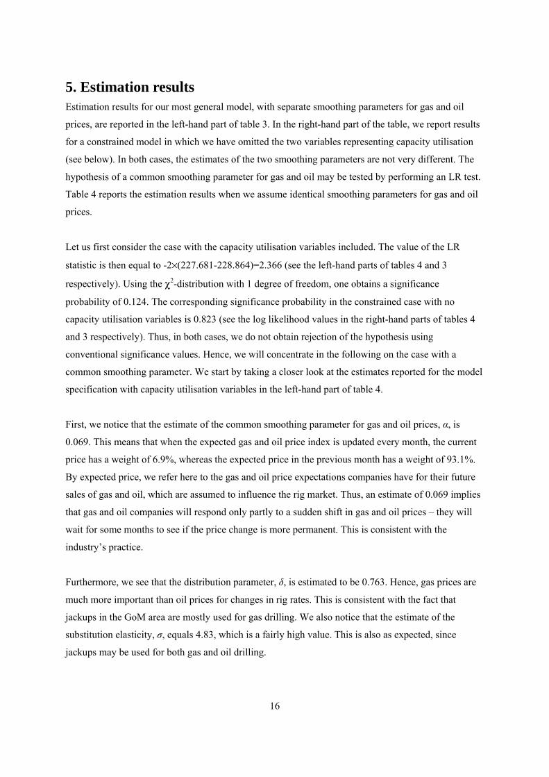
5. Estimation results Estimation results for our most general model, with separate smoothing parameters for gas and oil
prices, are reported in the left-hand part of table 3. In the right-hand part of the table, we report results
for a constrained model in which we have omitted the two variables representing capacity utilisation
(see below). In both cases, the estimates of the two smoothing parameters are not very different. The
hypothesis of a common smoothing parameter for gas and oil may be tested by performing an LR test.
Table 4 reports the estimation results when we assume identical smoothing parameters for gas and oil
prices.
Let us first consider the case with the capacity utilisation variables included. The value of the LR
statistic is then equal to -2×(227.681-228.864)=2.366 (see the left-hand parts of tables 4 and 3
respectively). Using the χ2-distribution with 1 degree of freedom, one obtains a significance
probability of 0.124. The corresponding significance probability in the constrained case with no
capacity utilisation variables is 0.823 (see the log likelihood values in the right-hand parts of tables 4
and 3 respectively). Thus, in both cases, we do not obtain rejection of the hypothesis using
conventional significance values. Hence, we will concentrate in the following on the case with a
common smoothing parameter. We start by taking a closer look at the estimates reported for the model
specification with capacity utilisation variables in the left-hand part of table 4.
First, we notice that the estimate of the common smoothing parameter for gas and oil prices, α, is
0.069. This means that when the expected gas and oil price index is updated every month, the current
price has a weight of 6.9%, whereas the expected price in the previous month has a weight of 93.1%.
By expected price, we refer here to the gas and oil price expectations companies have for their future
sales of gas and oil, which are assumed to influence the rig market. Thus, an estimate of 0.069 implies
that gas and oil companies will respond only partly to a sudden shift in gas and oil prices – they will
wait for some months to see if the price change is more permanent. This is consistent with the
industry’s practice.
Furthermore, we see that the distribution parameter, δ, is estimated to be 0.763. Hence, gas prices are
much more important than oil prices for changes in rig rates. This is consistent with the fact that
jackups in the GoM area are mostly used for gas drilling. We also notice that the estimate of the
substitution elasticity, σ, equals 4.83, which is a fairly high value. This is also as expected, since
jackups may be used for both gas and oil drilling.
17
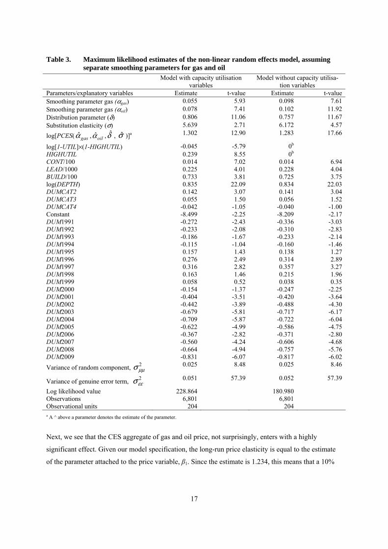
Table 3. Maximum likelihood estimates of the non-linear random effects model, assuming separate smoothing parameters for gas and oil
Model with capacity utilisation variables
Model without capacity utilisa-tion variables
Parameters/explanatory variables Estimate t-value Estimate t-value Smoothing parameter gas (αgas) 0.055 5.93 0.098 7.61 Smoothing parameter gas (αoil) 0.078 7.41 0.102 11.92 Distribution parameter (δ) 0.806 11.06 0.757 11.67 Substitution elasticity (σ) 5.639 2.71 6.172 4.57
log[PCES( ˆgasα , ˆoilα , δ̂ , σ̂ )]a 1.302 12.90 1.283 17.66
log[1-UTIL]×(1-HIGHUTIL) -0.045 -5.79 0b HIGHUTIL 0.239 8.55 0b CONT/100 0.014 7.02 0.014 6.94 LEAD/1000 0.225 4.01 0.228 4.04 BUILD/100 0.733 3.81 0.725 3.75 log(DEPTH) 0.835 22.09 0.834 22.03 DUMCAT2 0.142 3.07 0.141 3.04 DUMCAT3 0.055 1.50 0.056 1.52 DUMCAT4 -0.042 -1.05 -0.040 -1.00 Constant -8.499 -2.25 -8.209 -2.17 DUM1991 -0.272 -2.43 -0.336 -3.03 DUM1992 -0.233 -2.08 -0.310 -2.83 DUM1993 -0.186 -1.67 -0.233 -2.14 DUM1994 -0.115 -1.04 -0.160 -1.46 DUM1995 0.157 1.43 0.138 1.27 DUM1996 0.276 2.49 0.314 2.89 DUM1997 0.316 2.82 0.357 3.27 DUM1998 0.163 1.46 0.215 1.96 DUM1999 0.058 0.52 0.038 0.35 DUM2000 -0.154 -1.37 -0.247 -2.25 DUM2001 -0.404 -3.51 -0.420 -3.64 DUM2002 -0.442 -3.89 -0.488 -4.30 DUM2003 -0.679 -5.81 -0.717 -6.17 DUM2004 -0.709 -5.87 -0.722 -6.04 DUM2005 -0.622 -4.99 -0.586 -4.75 DUM2006 -0.367 -2.82 -0.371 -2.80 DUM2007 -0.560 -4.24 -0.606 -4.68 DUM2008 -0.664 -4.94 -0.757 -5.76 DUM2009 -0.831 -6.07 -0.817 -6.02
Variance of random component, 2μμσ 0.025 8.48 0.025 8.46
Variance of genuine error term, 2εεσ 0.051 57.39 0.052 57.39
Log likelihood value 228.864 180.980 Observations 6,801 6,801 Observational units 204 204 a A ^ above a parameter denotes the estimate of the parameter.
Next, we see that the CES aggregate of gas and oil price, not surprisingly, enters with a highly
significant effect. Given our model specification, the long-run price elasticity is equal to the estimate
of the parameter attached to the price variable, β1. Since the estimate is 1.234, this means that a 10%
18
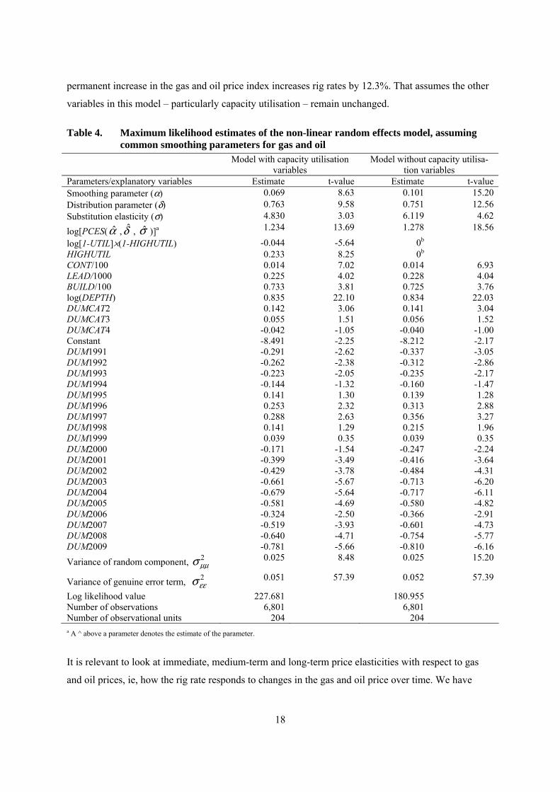
permanent increase in the gas and oil price index increases rig rates by 12.3%. That assumes the other
variables in this model – particularly capacity utilisation – remain unchanged.
Table 4. Maximum likelihood estimates of the non-linear random effects model, assuming common smoothing parameters for gas and oil
Model with capacity utilisation variables
Model without capacity utilisa-tion variables
Parameters/explanatory variables Estimate t-value Estimate t-value Smoothing parameter (α) 0.069 8.63 0.101 15.20 Distribution parameter (δ) 0.763 9.58 0.751 12.56 Substitution elasticity (σ) 4.830 3.03 6.119 4.62
log[PCES(α̂ , δ̂ , σ̂ )]a 1.234 13.69 1.278 18.56
log[1-UTIL]×(1-HIGHUTIL) -0.044 -5.64 0b HIGHUTIL 0.233 8.25 0b CONT/100 0.014 7.02 0.014 6.93 LEAD/1000 0.225 4.02 0.228 4.04 BUILD/100 0.733 3.81 0.725 3.76 log(DEPTH) 0.835 22.10 0.834 22.03 DUMCAT2 0.142 3.06 0.141 3.04 DUMCAT3 0.055 1.51 0.056 1.52 DUMCAT4 -0.042 -1.05 -0.040 -1.00 Constant -8.491 -2.25 -8.212 -2.17 DUM1991 -0.291 -2.62 -0.337 -3.05 DUM1992 -0.262 -2.38 -0.312 -2.86 DUM1993 -0.223 -2.05 -0.235 -2.17 DUM1994 -0.144 -1.32 -0.160 -1.47 DUM1995 0.141 1.30 0.139 1.28 DUM1996 0.253 2.32 0.313 2.88 DUM1997 0.288 2.63 0.356 3.27 DUM1998 0.141 1.29 0.215 1.96 DUM1999 0.039 0.35 0.039 0.35 DUM2000 -0.171 -1.54 -0.247 -2.24 DUM2001 -0.399 -3.49 -0.416 -3.64 DUM2002 -0.429 -3.78 -0.484 -4.31 DUM2003 -0.661 -5.67 -0.713 -6.20 DUM2004 -0.679 -5.64 -0.717 -6.11 DUM2005 -0.581 -4.69 -0.580 -4.82 DUM2006 -0.324 -2.50 -0.366 -2.91 DUM2007 -0.519 -3.93 -0.601 -4.73 DUM2008 -0.640 -4.71 -0.754 -5.77 DUM2009 -0.781 -5.66 -0.810 -6.16
Variance of random component, 2μμσ 0.025 8.48 0.025 15.20
Variance of genuine error term, 2εεσ 0.051 57.39 0.052 57.39
Log likelihood value 227.681 180.955 Number of observations 6,801 6,801 Number of observational units 204 204 a A ^ above a parameter denotes the estimate of the parameter.
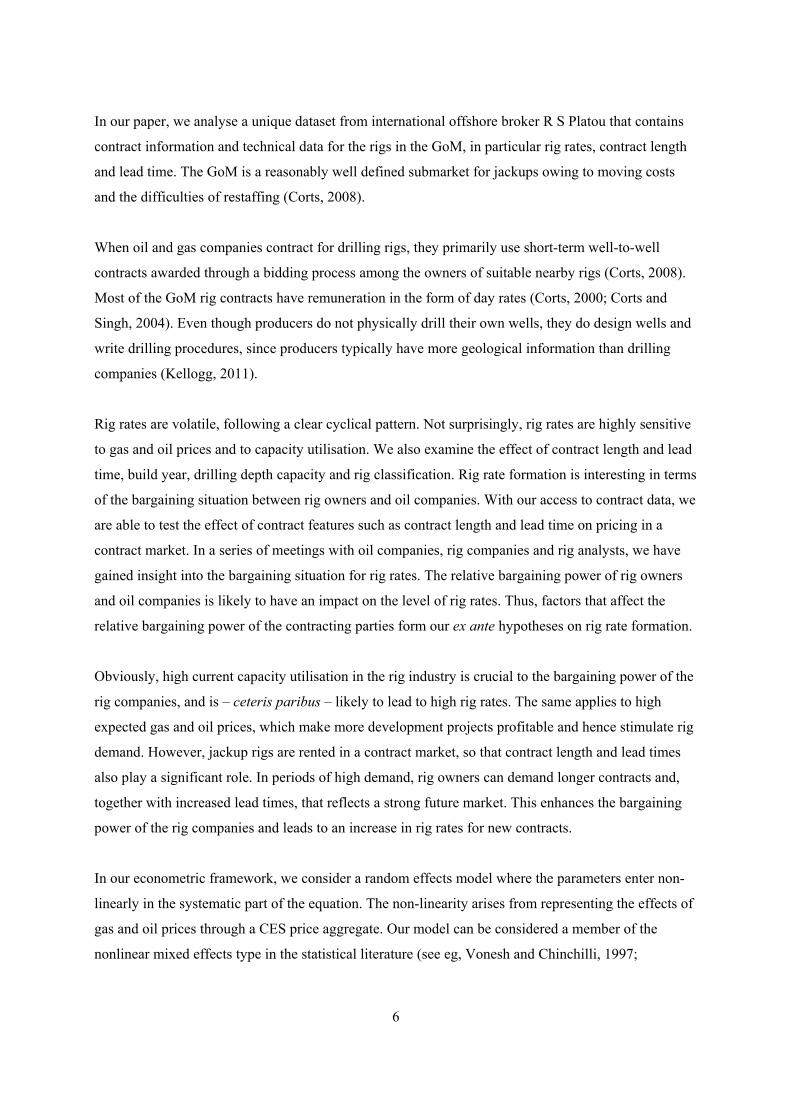
It is relevant to look at immediate, medium-term and long-term price elasticities with respect to gas
and oil prices, ie, how the rig rate responds to changes in the gas and oil price over time. We have
19
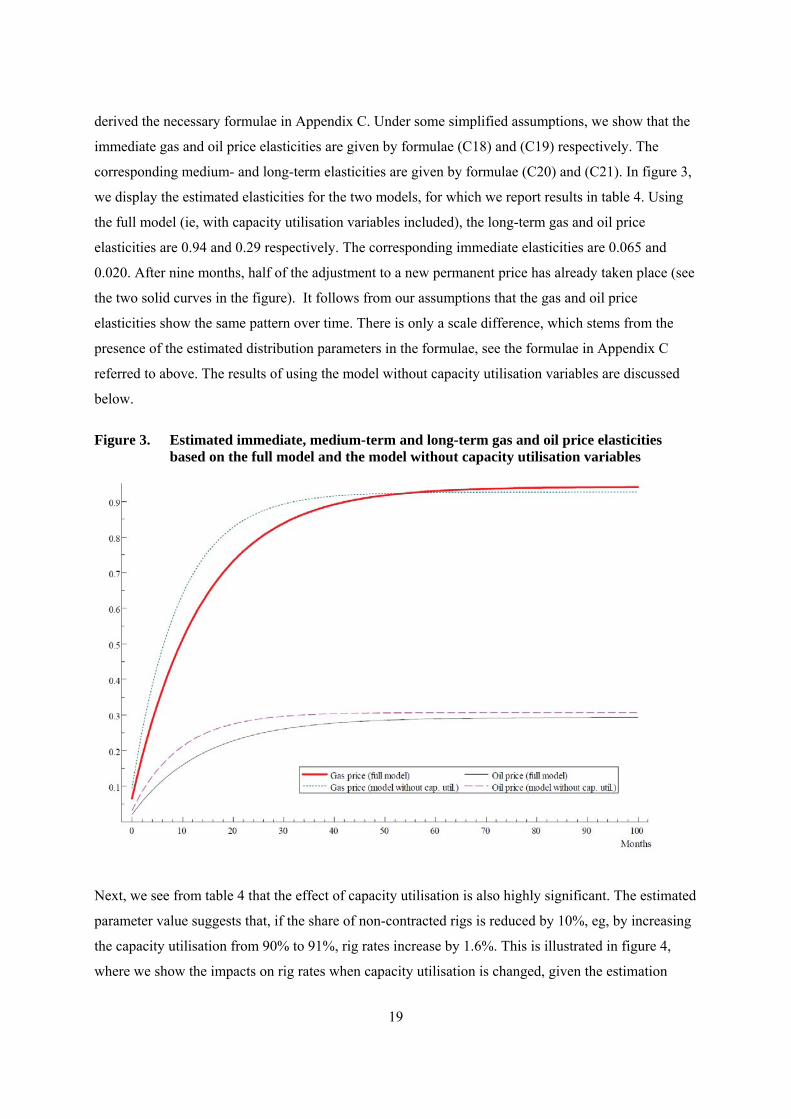
derived the necessary formulae in Appendix C. Under some simplified assumptions, we show that the
immediate gas and oil price elasticities are given by formulae (C18) and (C19) respectively. The
corresponding medium- and long-term elasticities are given by formulae (C20) and (C21). In figure 3,
we display the estimated elasticities for the two models, for which we report results in table 4. Using
the full model (ie, with capacity utilisation variables included), the long-term gas and oil price
elasticities are 0.94 and 0.29 respectively. The corresponding immediate elasticities are 0.065 and
0.020. After nine months, half of the adjustment to a new permanent price has already taken place (see
the two solid curves in the figure). It follows from our assumptions that the gas and oil price
elasticities show the same pattern over time. There is only a scale difference, which stems from the
presence of the estimated distribution parameters in the formulae, see the formulae in Appendix C
referred to above. The results of using the model without capacity utilisation variables are discussed
below.
Figure 3. Estimated immediate, medium-term and long-term gas and oil price elasticities based on the full model and the model without capacity utilisation variables
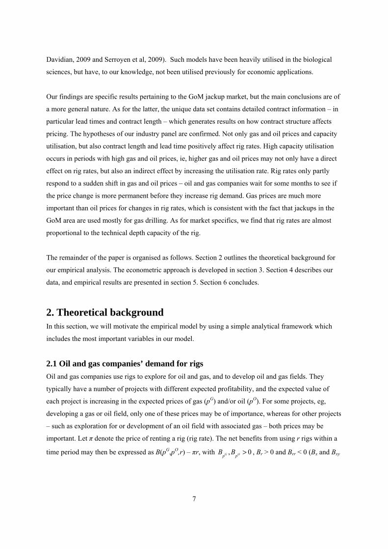
Next, we see from table 4 that the effect of capacity utilisation is also highly significant. The estimated
parameter value suggests that, if the share of non-contracted rigs is reduced by 10%, eg, by increasing
the capacity utilisation from 90% to 91%, rig rates increase by 1.6%. This is illustrated in figure 4,
where we show the impacts on rig rates when capacity utilisation is changed, given the estimation
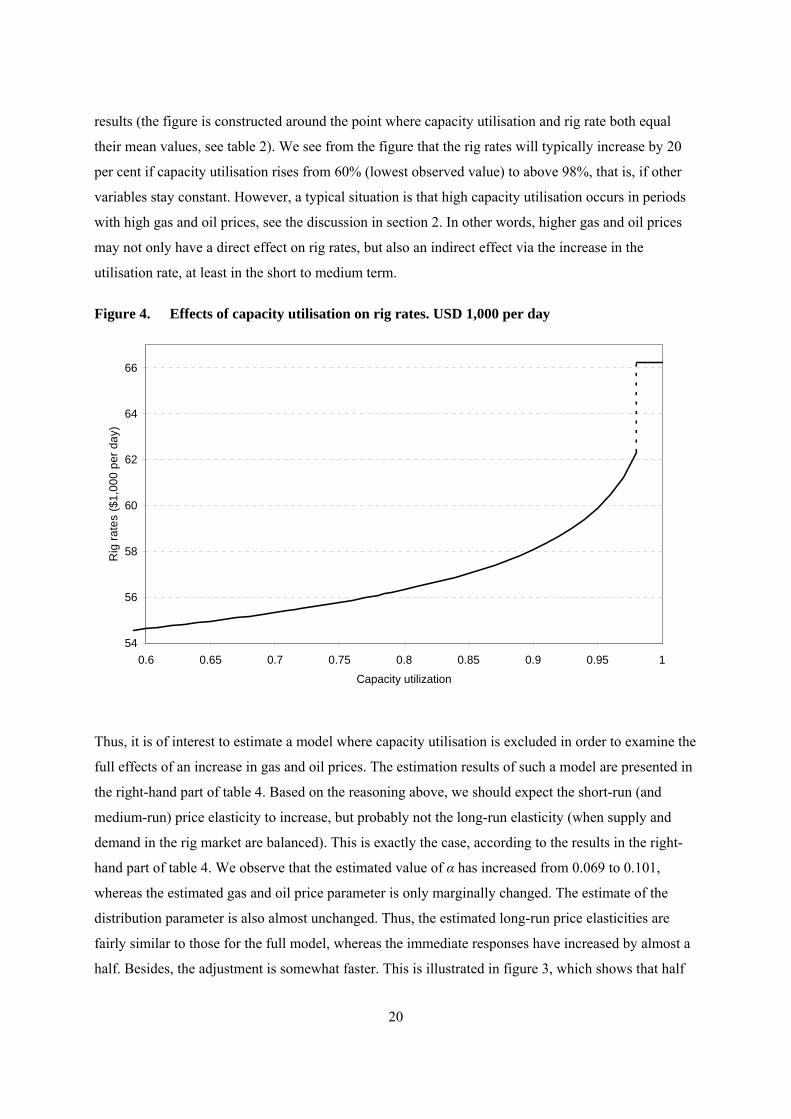
20
results (the figure is constructed around the point where capacity utilisation and rig rate both equal
their mean values, see table 2). We see from the figure that the rig rates will typically increase by 20
per cent if capacity utilisation rises from 60% (lowest observed value) to above 98%, that is, if other
variables stay constant. However, a typical situation is that high capacity utilisation occurs in periods
with high gas and oil prices, see the discussion in section 2. In other words, higher gas and oil prices
may not only have a direct effect on rig rates, but also an indirect effect via the increase in the
utilisation rate, at least in the short to medium term.
Figure 4. Effects of capacity utilisation on rig rates. USD 1,000 per day
54
56
58
60
62
64
66
0.6 0.65 0.7 0.75 0.8 0.85 0.9 0.95 1
Capacity utilization
Rig
rat
es
($1,
00
0 p
er d
ay)
Thus, it is of interest to estimate a model where capacity utilisation is excluded in order to examine the
full effects of an increase in gas and oil prices. The estimation results of such a model are presented in
the right-hand part of table 4. Based on the reasoning above, we should expect the short-run (and
medium-run) price elasticity to increase, but probably not the long-run elasticity (when supply and
demand in the rig market are balanced). This is exactly the case, according to the results in the right-
hand part of table 4. We observe that the estimated value of α has increased from 0.069 to 0.101,
whereas the estimated gas and oil price parameter is only marginally changed. The estimate of the
distribution parameter is also almost unchanged. Thus, the estimated long-run price elasticities are
fairly similar to those for the full model, whereas the immediate responses have increased by almost a
half. Besides, the adjustment is somewhat faster. This is illustrated in figure 3, which shows that half
21
of the adjustment to permanently higher gas and oil prices occurs within six months (see the dotted
curves). However, we see from the log likelihood values of the two models in table 4 that a large and
significant drop in explanatory power is obtained when the parameters attached to the two capacity
utilisation variables are forced to be zero. Thus, capacity utilisation is undoubtedly an important factor
in determining rig rates.
The other (non-dummy) variables are also highly significant, and the estimated parameter values are
almost the same in the two panels of table 4, ie, with and without capacity utilisation as a variable. In
particular, we notice that rigs able to drill at greater depths are significantly more expensive than rigs
only able to operate in shallower waters. The estimated parameter value indicates an elasticity of 0.84,
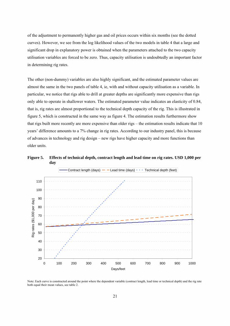
that is, rig rates are almost proportional to the technical depth capacity of the rig. This is illustrated in
figure 5, which is constructed in the same way as figure 4. The estimation results furthermore show
that rigs built more recently are more expensive than older rigs – the estimation results indicate that 10
years’ difference amounts to a 7% change in rig rates. According to our industry panel, this is because
of advances in technology and rig design – new rigs have higher capacity and more functions than
older units.
Figure 5. Effects of technical depth, contract length and lead time on rig rates. USD 1,000 per day
20
30
40
50
60
70
80
90
100
110
0 100 200 300 400 500 600 700 800 900 1000
Days/feet
Rig
rat
es
($1,
000
pe
r d
ay)
Contract length (days) Lead time (days) Technical depth (feet)
Note: Each curve is constructed around the point where the dependent variable (contract length, lead time or technical depth) and the rig rate both equal their mean values, see table 2.
22
Figure 5 furthermore shows that both the length of the contract and the lead time, ie, the time from the
contract is signed until the rental period starts, have significant, positive effects on the rig rate. In a
period of increasing demand, rig availability is lower and operators are being forced to sign contracts
in advance. The rig companies’ contract backlog increases, their relative bargaining power is enhanced
and rig rates rise. The estimated value indicates that, when the lead time increases by six months, the
day rate goes up by around 3.8%. Similarly, according to these estimations (see figure 5), we find that
extending the contract length by six months increases the day rate by around 2.6%. In periods of high
demand, rig owners can demand longer contracts and, together with increased lead times, this reflects
a strong future market.
Some but not all of the rig category dummies are significant.12 According to our results, the most
valuable jackup category seems to be the independent leg slot jackup, after controlling for other
characteristics such as drilling depth and build year. The rig rate for this category is estimated to be
14% higher than for the independent leg cantilever jackup. According to the industry specialists we
have interviewed, this is somewhat surprising, since this rig category is not being built anymore. Note,
however, that differences in both build year and technical depth are captured by separate variables.
The limited number of rigs available in this category is also put forward as an explanation for this
result (10% of the sample, see table 2).13
6. Conclusions The relative bargaining power of rig owners and oil companies is likely to have an impact on the level
of rig rates. Thus, factors that affect the relative bargaining power of the contracting parties form our
ex ante hypotheses on rig rate formation. A unique dataset from the GoM rig market allows us to test
the relationship between contract data and pricing in a contract market.
Our econometric analysis of GoM jackup rig rates confirms the hypotheses of our industry panel.
Obviously, high current capacity utilisation in the rig industry is crucial to the bargaining power of the
rig companies, and leads to high rig rates. The same applies to high expected gas and oil prices, which
stimulate gas and oil development projects and hence increase rig demand. Consistent with industry
practice, however, petroleum companies only partly respond to sudden shifts in the gas and oil prices –
12 Whereas the log likelihood value is 227.681 (see the left-hand part of table 3) in our main model, it is 220.797 in the model specification without rig category dummies. Thus, using an LR-statistic, the hypothesis that the three slope parameters attached to these dummies are zero is rejected at the 1% significance level. 13 We have also performed separate estimations for rig types 1 and 3, which together account for 75% of the observations. The main conclusions carry over. The estimation results can be made available by the authors upon request.

23
they wait for some months to see if the price change is more permanent. Consistent with the fact that
jackups in the GoM area are used mostly for gas drilling, we find that gas prices are much more
important than oil prices for changes in rig rates.
Since this is a contract market, contract length and lead times also play a significant role. In periods of
high demand, rig owners can demand longer contracts and, together with increased lead times, this
reflects a strong future market. The increase in the contract backlog enhances the bargaining power of
the rig companies and leads to a rise in rig rates for new contracts.
In this study, we have considered a non-linear random effects model and estimated all the unknown
parameters by maximum likelihood. Models of these types have been heavily utilised in the biological
sciences. Even though they are relevant for several economic applications, too, we are not aware of
earlier econometric studies utilising such models.
In our estimations, we have implicitly treated the GoM area as a closed market, since capacity
utilisation and gas prices in other parts of the world have not been included. This could be a weakness
with our analysis, as some movement of rigs takes place between areas. Since it is quite costly to move
rigs over large distances, however, we believe that this omission is of minor importance.
Whereas jackups are mainly used in shallow water (and on land), oil and gas companies use floaters
when they drill in deep water. Whether the market for renting floaters has similar characteristics as the
jackup market is an interesting question we leave for future research. Floaters are typically rented for
longer periods than jackups, and thus the backlog of future contracts may be even more important for
the rig rates.
24
References
Aune, Finn R., Klaus Mohn, Petter Osmundsen, and Knut E. Rosendahl. 2010. “Financial Market
Pressure, Tacit Collusion and Oil Price Formation.” Energy Economics 32: 389-398.
Boyce, John R., and Linda Nøstbakken. 2011. “Exploration and Development of U.S. Oil and Gas
Fields.” Journal of Economics Dynamics and Control, 35: 891-908.
Corts, Kenneth S. 2000. “Turnkey Contracts as a Response to Incentive Problems: Evidence from the
Offshore Drilling Industry. ” Working paper, Harvard University.
Corts, Kenneth S. 2008. “Stacking the Deck: Idling and Reactivation of Capacity in Offshore
Drilling.” Journal of Economics and Management Strategy 17(2): 271-294.
Corts, Kenneth S., and Jasjit Singh. 2004. “The Effect of Repeated Interaction on Contract Choice:
Evidence from Offshore Drilling.” Journal of Law, Economics, and Organization 20 (1): 230-260.
Davidian, Marie. 2009. “Non-linear Mixed Effects Models. Chapter 5 in Longitudinal Data Analysis,
edited by Garret Fitzmaurice, Marie Davidian, Geert Verbeke, and Geert Molenberghs, 107-142 .
Chapman & Hall.
EIA, 2011. “Annual Energy Review 2010”. US Energy Information Administration, October 2011.
Kellogg, Ryan. 2011. “Learning by Drilling: Interfirm Learning and Relationship Persistence in the
Texas Oilpatch.” The Quarterly Journal of Economics 126: 1961-2004.
Koyck, Leendert M. 1954. “Distributed Lags and Investment Analysis.” Amsterdam: North-Holland.
Osmundsen, Petter, Kristin H. Roll, and Ragnar Tveterås. 2010. “Exploration Drilling Productivity at
the Norwegian Shelf.” Journal of Petroleum Science and Engineering 73: 122-128.
Osmundsen, Petter, Kristin H. Roll and Ragnar Tveterås. 2012. “Drilling Speed - the Relevance of
Experience.” Energy Economics 34: 786-794.

25
Ringlund, Guro B., Knut E. Rosendahl and Terje Skjerpen 2008. “Does oilrig activity react to oil price
changes? An empirical investigation.” Energy Economics 30; 371-396.
Serroyen, Jan, Geert Molenberghs, Geert Verbeke, and Marie Davidian. 2009. “Nonlinear Models for
Longitudinal Data.” American Statistician 63: 378-388.
Vonesh, Edward F., and Vernon M. Chinchilli. 1997: Linear and Nonlinear Models for the Analysis of
Repeated Measurements. Marcel Dekker.
26
Appendix A. Further information on data
Table A1. The unbalancedness of the panel dataa
No of obs for an obs unit
Number of rigs being obs the
indicated no of times No of obs
No of obs for an obs unit
Number of rigs being obs the
indicated no of times No of obs
1 11 11 2 6 12 3 7 21 4 4 16 5 6 30 6 3 18 7 3 21 8 7 56 9 0 0 10 3 30 11 4 44 12 3 36 13 2 26 14 1 14 15 3 45 16 4 64 17 2 34 18 0 0 19 2 38 20 4 80 21 1 21 22 3 66 23 2 46 24 1 24 25 0 0 26 2 52 27 3 81 28 0 0 29 2 58 30 1 30 31 2 62 32 1 32 33 5 165 34 1 34 35 3 105 36 1 36 37 8 296 38 3 114 39 0 0 40 5 200 41 2 82 42 4 168 43 3 129 44 7 308 45 2 90 46 2 92 47 5 235 48 4 192 49 5 245 50 2 100 51 2 102 52 2 104 53 3 159 54 3 162 55 3 165 56 3 168 57 5 285 58 2 116 59 1 59 60 1 60 61 1 61 62 3 186 63 0 0 64 1 64 65 2 130 66 0 0 67 0 0 68 1 68 69 3 207 70 0 0 71 0 0 72 0 0 73 1 73 74 4 296 75 0 0 76 0 0 77 1 77 78 0 0 79 0 0 80 2 160 81 0 0 82 0 0 83 0 0 84 0 0 85 0 0 86 2 172 87 1 87 88 0 0 89 1 89 90 0 0 91 0 0 92 1 92 a The total number of observational units and the total number of observations are 204 and 6,801, respectively.
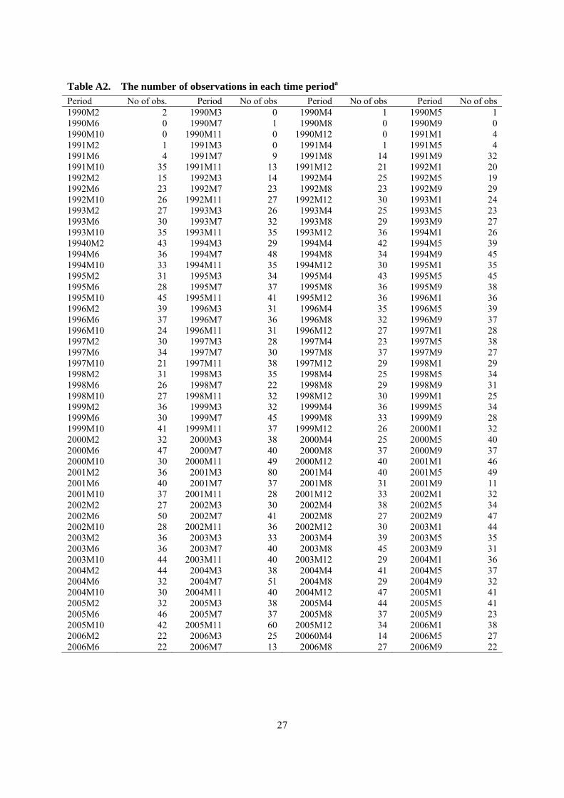
27
Table A2. The number of observations in each time perioda Period No of obs. Period No of obs Period No of obs Period No of obs 1990M2 2 1990M3 0 1990M4 1 1990M5 1 1990M6 0 1990M7 1 1990M8 0 1990M9 0 1990M10 0 1990M11 0 1990M12 0 1991M1 4 1991M2 1 1991M3 0 1991M4 1 1991M5 4 1991M6 4 1991M7 9 1991M8 14 1991M9 32 1991M10 35 1991M11 13 1991M12 21 1992M1 20 1992M2 15 1992M3 14 1992M4 25 1992M5 19 1992M6 23 1992M7 23 1992M8 23 1992M9 29 1992M10 26 1992M11 27 1992M12 30 1993M1 24 1993M2 27 1993M3 26 1993M4 25 1993M5 23 1993M6 30 1993M7 32 1993M8 29 1993M9 27 1993M10 35 1993M11 35 1993M12 36 1994M1 26 19940M2 43 1994M3 29 1994M4 42 1994M5 39 1994M6 36 1994M7 48 1994M8 34 1994M9 45 1994M10 33 1994M11 35 1994M12 30 1995M1 35 1995M2 31 1995M3 34 1995M4 43 1995M5 45 1995M6 28 1995M7 37 1995M8 36 1995M9 38 1995M10 45 1995M11 41 1995M12 36 1996M1 36 1996M2 39 1996M3 31 1996M4 35 1996M5 39 1996M6 37 1996M7 36 1996M8 32 1996M9 37 1996M10 24 1996M11 31 1996M12 27 1997M1 28 1997M2 30 1997M3 28 1997M4 23 1997M5 38 1997M6 34 1997M7 30 1997M8 37 1997M9 27 1997M10 21 1997M11 38 1997M12 29 1998M1 29 1998M2 31 1998M3 35 1998M4 25 1998M5 34 1998M6 26 1998M7 22 1998M8 29 1998M9 31 1998M10 27 1998M11 32 1998M12 30 1999M1 25 1999M2 36 1999M3 32 1999M4 36 1999M5 34 1999M6 30 1999M7 45 1999M8 33 1999M9 28 1999M10 41 1999M11 37 1999M12 26 2000M1 32 2000M2 32 2000M3 38 2000M4 25 2000M5 40 2000M6 47 2000M7 40 2000M8 37 2000M9 37 2000M10 30 2000M11 49 2000M12 40 2001M1 46 2001M2 36 2001M3 80 2001M4 40 2001M5 49 2001M6 40 2001M7 37 2001M8 31 2001M9 11 2001M10 37 2001M11 28 2001M12 33 2002M1 32 2002M2 27 2002M3 30 2002M4 38 2002M5 34 2002M6 50 2002M7 41 2002M8 27 2002M9 47 2002M10 28 2002M11 36 2002M12 30 2003M1 44 2003M2 36 2003M3 33 2003M4 39 2003M5 35 2003M6 36 2003M7 40 2003M8 45 2003M9 31 2003M10 44 2003M11 40 2003M12 29 2004M1 36 2004M2 44 2004M3 38 2004M4 41 2004M5 37 2004M6 32 2004M7 51 2004M8 29 2004M9 32 2004M10 30 2004M11 40 2004M12 47 2005M1 41 2005M2 32 2005M3 38 2005M4 44 2005M5 41 2005M6 46 2005M7 37 2005M8 37 2005M9 23 2005M10 42 2005M11 60 2005M12 34 2006M1 38 2006M2 22 2006M3 25 20060M4 14 2006M5 27 2006M6 22 2006M7 13 2006M8 27 2006M9 22
28
Table A2. (continued) Period No of obs Period No of obs Period No of obs Period No. of obs. 2006M10 18 2006M11 35 2006M12 28 2007M1 23 2007M2 16 2007M3 26 2007M4 27 2007M5 18 2007M6 23 2007M7 11 2007M8 21 2007M9 13 2007M10 28 2007M11 22 2007M12 20 2008M1 12 2008M2 25 2008M3 29 2008M4 32 2008M5 28 2008M6 25 2008M7 24 2008M8 17 2008M9 23 2008M10 25 2008M11 14 2008M12 20 2009M1 9 2009M2 10 2009M3 15 2009M4 11 2009M5 14 2009M6 5 2009M7 7 2009M8 6 2009M9 13 2009M10 3 a The total number of observations is 6,801.
Table A3. Rig categories involved General category description Rig category number used in current paper Independent leg cantilever jackups 1 Independent leg slot jackups 2 Mat supported cantilever jackups 3 Mat supported slot jackups 4
Figure A1. Capacity utilisation rates for jackups in the Gulf of Mexico area
1990 1995 2000 2005 2010
0.65
0.70
0.75
0.80
0.85
0.90
0.95
1.00
29
Figure A2. The oil price in current US dollars
Oil price in cuurent US dollars
1970 1975 1980 1985 1990 1995 2000 2005 2010
20
40
60
80
100
120
Oil price in cuurent US dollars
Figure A3. US natural gas wellhead price (dollars per thousand cubic feet)
1980 1985 1990 1995 2000 2005 2010
1
2
3
4
5
6
7
8
9
10
11
30
Figure A4. The price deflator – 2008=1
Deflator
1970 1975 1980 1985 1990 1995 2000 2005 2010
0.3
0.4
0.5
0.6
0.7
0.8
0.9
1.0 Deflator
31
Appendix B: Additional information on the grid search used to obtain starting values
Table B1. Parameter values used in the grid search
α δ σ 0.03 0.1 0.1 0.04 0.2 0.3 0.05 0.3 0.5 0.06 0.4 0.7 0.08 0.5 0.95 0.10 0.6 1.5 0.12 0.65 2 0.15 0.7 2.5 0.20 0.75 3 0.25 0.80 4 0.30 0.85 5 0.90 6 0.95 8 10 12 14 16 18 20
32
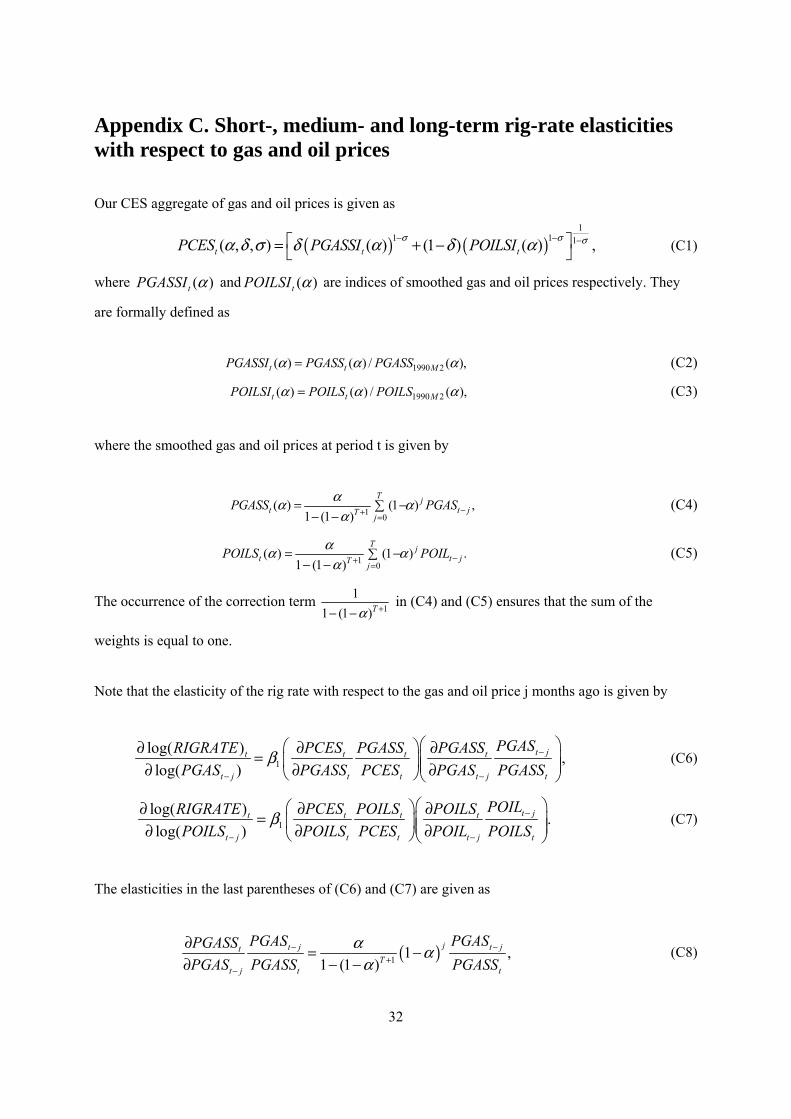
Appendix C. Short-, medium- and long-term rig-rate elasticities with respect to gas and oil prices
Our CES aggregate of gas and oil prices is given as
( ) ( )1
1 1 1( , , ) ( ) (1 ) ( ) ,t t tPCES PGASSI POILSIσ σ σα δ σ δ α δ α− − − = + − (C1)
where ( )tPGASSI α and ( )tPOILSI α are indices of smoothed gas and oil prices respectively. They
are formally defined as
1990 2( ) ( ) / ( ),t t MPGASSI PGASS PGASSα α α= (C2)
1990 2( ) ( ) / ( ),t t MPOILSI POILS POILSα α α= (C3)
where the smoothed gas and oil prices at period t is given by
1
0( ) (1 ) ,
1 (1 )
Tj
t t jTj
PGASS PGASαα α
α −+ == −
− − (C4)
10
( ) (1 ) .1 (1 )
Tj
t t jTj
POILS POILαα α
α −+ == −
− − (C5)
The occurrence of the correction term 1
1
1 (1 )Tα +− − in (C4) and (C5) ensures that the sum of the
weights is equal to one.
Note that the elasticity of the rig rate with respect to the gas and oil price j months ago is given by
1
log( ),
log( )t jt t t t
t j t t t j t
PGASRIGRATE PCES PGASS PGASS
PGAS PGASS PCES PGAS PGASSβ −
− −
∂ ∂ ∂= ∂ ∂ ∂ (C6)
1
log( ).
log( )t jt t t t
t j t t t j t
POILRIGRATE PCES POILS POILS
POILS POILS PCES POIL POILSβ −
− −
∂ ∂ ∂= ∂ ∂ ∂ (C7)
The elasticities in the last parentheses of (C6) and (C7) are given as
( )11 ,
1 (1 )jt j t jt
Tt j t t
PGAS PGASPGASS
PGAS PGASS PGASS
α αα
− −+
−
∂ = −∂ − −
(C8)
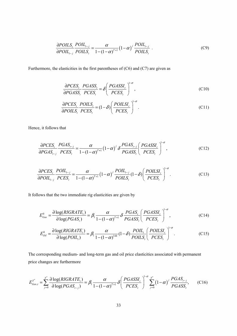
33
( )11
1 (1 )jt j t jt
Tt j t t
POIL POILPOILS
POIL POILS POILS
α αα
− −+
−
∂ = −∂ − −
. (C9)
Furthermore, the elasticities in the first parentheses of (C6) and (C7) are given as
1
,t t t
t t t
PCES PGASS PGASSI
PGASS PCES PCES
σ
δ−
∂ = ∂ (C10)
1
(1 ) .t t t
t t t
PCES POILS POILSI
POILS PCES PCES
σ
δ−
∂ = − ∂ (C11)
Hence, it follows that
( )1
11 ,
1 (1 )
jt j t jt tT
t j t t t
PGAS PGASPCES PGASSI
PGAS PCES PGASS PCES
σα α δ
α
−− −
+−
∂ = − ∂ − − (C12)
( )1
11 (1 ) .
1 (1 )
jt j t jt tT
t j t t t
POIL POILPCES POILSI
POIL PCES POILS PCES
σα α δ
α
−− −
+−
∂ = − − ∂ − − (C13)
It follows that the two immediate rig elasticities are given by
1
01 1
log( ),
log( ) 1 (1 )t t t
Gas Tt t t
RIGRATE PGAS PGASSIE
PGAS PGASS PCES
σαβ δ
α
−
+
∂= = ∂ − − (C14)
1
01 144
log( )(1 ) .
log( ) 1 (1 )t t t
Oilt t t
RIGRATE POIL POILSIE
POIL POILS PCES
σαβ δ
α
− ∂= = − ∂ − −
(C15)
The corresponding medium- and long-term gas and oil price elasticities associated with permanent
price changes are furthermore
( )* *
*
1
, 1 10 0
log( )1 ,
log( ) 1 (1 )
T Tj t jT t t
Gas t Tj jt j t t
PGASRIGRATE PGASSIE
PGAS PCES PGASS
σαβ δ α
α
−−
+= =−
∂= = − ∂ − − (C16)
34
( )* *
*
1
, 1 10 0
log( )(1 ) 1 ,
log( ) 1 (1 )
T Tj t jT t t
Oil t Tj jt j t t
POILRIGRATE POILSIE
POIL PCES POILS
σαβ δ α
α
−−
+= =−
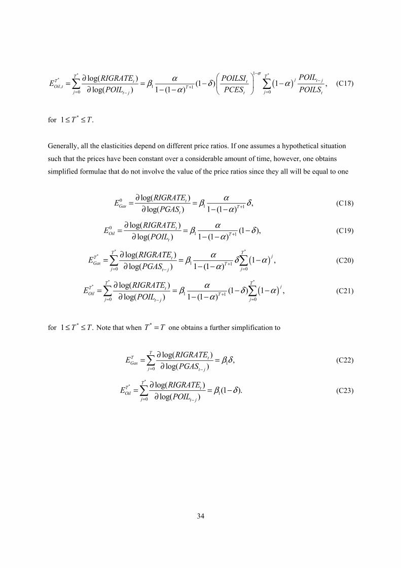
∂= = − − ∂ − − (C17)
for *1 .T T≤ ≤
Generally, all the elasticities depend on different price ratios. If one assumes a hypothetical situation
such that the prices have been constant over a considerable amount of time, however, one obtains
simplified formulae that do not involve the value of the price ratios since they all will be equal to one
01 1
log( ),
log( ) 1 (1 )t
Gas Tt
RIGRATEE
PGAS
αβ δα +
∂= =∂ − −
(C18)
01 1
log( )(1 ),
log( ) 1 (1 )t
Oil Tt
RIGRATEE
POIL
αβ δα +
∂= = −∂ − −
(C19)
( )* *
*
1 10 0
log( )1 ,
log( ) 1 (1 )
T TjT t
Gas Tj jt j
RIGRATEE
PGAS
αβ δ αα +
= =−
∂= = −∂ − − (C20)
( )* *
*
1 10 0
log( )(1 ) 1 ,
log( ) 1 (1 )
T TjT t
Oil Tj jt j
RIGRATEE
POIL
αβ δ αα +
= =−
∂= = − −∂ − − (C21)
for *1 .T T≤ ≤ Note that when *T T= one obtains a further simplification to
10
log( ),
log( )
TT tGas
j t j
RIGRATEE
PGASβ δ
= −
∂= =∂ (C22)
**
10
log( )(1 ).
log( )
TT tOil
j t j
RIGRATEE
POILβ δ
= −
∂= = −∂ (C23)

Statistics Norway
Oslo:PO Box 8131 DeptNO-0033 OsloTelephone: + 47 21 09 00 00Telefax: + 47 21 09 00 40
Kongsvinger:NO-2225 KongsvingerTelephone: + 47 62 88 50 00Telefax: + 47 62 88 50 30
E-mail: [email protected]: www.ssb.no
ISSN 0809-733X
Returadresse:Statistisk sentralbyråNO-2225 KongsvingerB