Embed Size (px)
Citation preview
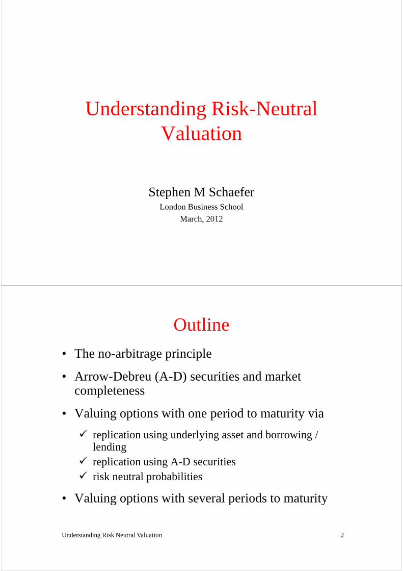
Understanding Risk-Neutral ValuationValuation
Stephen M SchaeferLondon Business School
March, 2012
Outline
• The no-arbitrage principle
• Arrow-Debreu (A-D) securities and market completeness
• Valuing options with one period to maturity via
Understanding Risk Neutral Valuation 2
� replication using underlying asset and borrowing / lending
� replication using A-D securities � risk neutral probabilities
• Valuing options with several periods to maturity
No-arbitrage pricing
Understanding Risk Neutral Valuation 3
No-arbitrage pricing
Arbitrage (Definition)• An arbitrage opportunity is one which:
a.Requires no invested capital
b.Provides a positive profit with 100% probability
• Or (slightly more generally)
a.Requires no invested capital,
b.Provides a positive profit with a positive probability and
Understanding Risk Neutral Valuation 4
b.Provides a positive profit with a positive probability and has a zero probability of a loss.
• Anyone who prefers more to less would engage in arbitrage because it represents “something for nothing”
• Therefore: in any competitive marketthere should be no arbitrage
“No-Arbitrage Pricing”
• Although absence of arbitrage is simply a necessary requirement for equilibrium it is in some cases sufficient to allow us to price one security in terms of another
• Idea: assets / portfolios with the same cash flows in each
Understanding Risk Neutral Valuation 5
• Idea: assets / portfolios with the same cash flows in each state must have the same price
• Pricing via no-arbitrage is relative pricing: we calculate the price on one security in terms of the prices of others.
Example: Valuing a Call option
Understanding Risk Neutral Valuation 6
Example: Valuing a Call option
The next steps …• We will use three approachesto value the same call
option that matures in one periodwhere the price of the underlying stock follows a binomial process1. Replication with stock and bond2. Replication with Arrow-Debreu (A-D) securities3. “Risk-Neutral” valuation
Understanding Risk Neutral Valuation 7
3. “Risk-Neutral” valuation
• Later we see how to deal with an option that matures in more than one period� in that case we will have to revise the replicating portfolio
over time� this “dynamic replication” (or “dynamic hedging”)
strategy is the key feature of option pricing
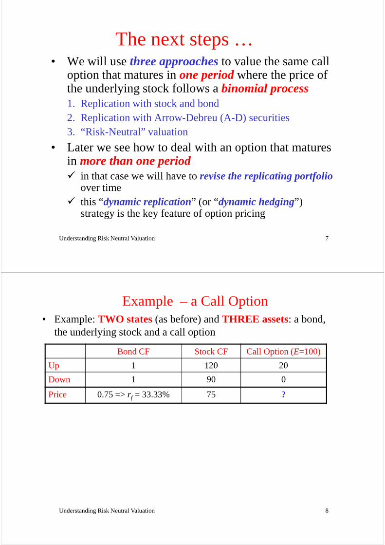
Example – a Call Option• Example: TWO states(as before) and THREE assets: a bond,
the underlying stock and a call option
Bond CF Stock CF Call Option (E=100)
Up 1 120 20
Down 1 90 0
Price 0.75 => rf = 33.33% 75 ?
Understanding Risk Neutral Valuation 8
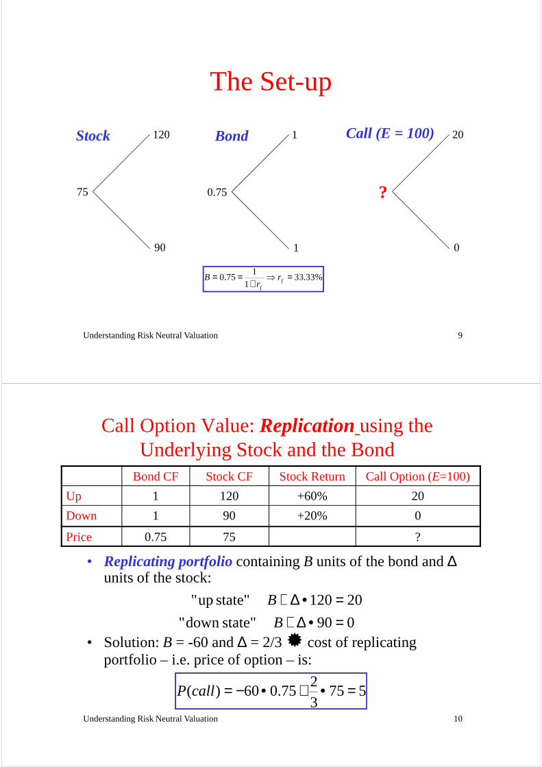
The Set-up
120
75
Stock 1
0.75
Bond 20
?
Call (E = 100)
Understanding Risk Neutral Valuation 9
90
75
1
0.75
0
?
10.75 33.33%
1 ff
B rr
= = ⇒ =+
Call Option Value: Replicationusing the Underlying Stock and the Bond
Bond CF Stock CF Stock Return Call Option (E=100)
Up 1 120 +60% 20
Down 1 90 +20% 0
Price 0.75 75 ?
• Replicating portfoliocontaining B units of the bond and ∆units of the stock:
Understanding Risk Neutral Valuation 10
units of the stock:
090 state"down "
20120 state" up"
=•∆+=•∆+
B
B
• Solution: B = -60 and ∆ = 2/3 � cost of replicating portfolio – i.e. price of option – is:
57532
75.060)( =•+•−=callP
Call Option Value: Replication using the Underlying Stock and the Bond
• Note: the portfolio that replicates a call option contains:
� the underlying stock
� borrowing
• the call valueis then just the cost of this portfolio
Understanding Risk Neutral Valuation 11
• the call valueis then just the cost of this portfolio
• This fact will be useful when we come to look at the Black-Scholes model.
Arrow-Debreu Securities and the
Understanding Risk Neutral Valuation 12
Arrow-Debreu Securities and the fundamental pricing relation in finance
Arrow-Debreu [A-D] Securities
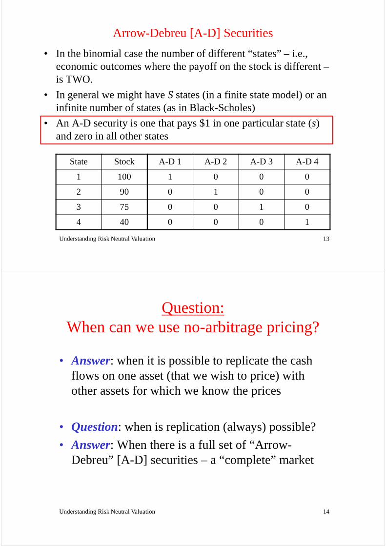
• In the binomial case the number of different “states” – i.e., economic outcomes where the payoff on the stock is different –is TWO.
• In general we might have S states (in a finite state model) or an infinite number of states (as in Black-Scholes)
• An A-D security is one that pays $1 in one particular state (s) and zero in all other states
Understanding Risk Neutral Valuation 13
and zero in all other states
State Stock A-D 1 A-D 2 A-D 3 A-D 4
1 100 1 0 0 0
2 90 0 1 0 0
3 75 0 0 1 0
4 40 0 0 0 1
Question:When can we use no-arbitrage pricing?
• Answer: when it is possible to replicate the cash flows on one asset (that we wish to price) with other assets for which we know the prices
Understanding Risk Neutral Valuation 14
• Question: when is replication (always) possible?
• Answer: When there is a full set of “Arrow-Debreu” [A-D] securities – a “complete” market
Complete markets and A-D Securities
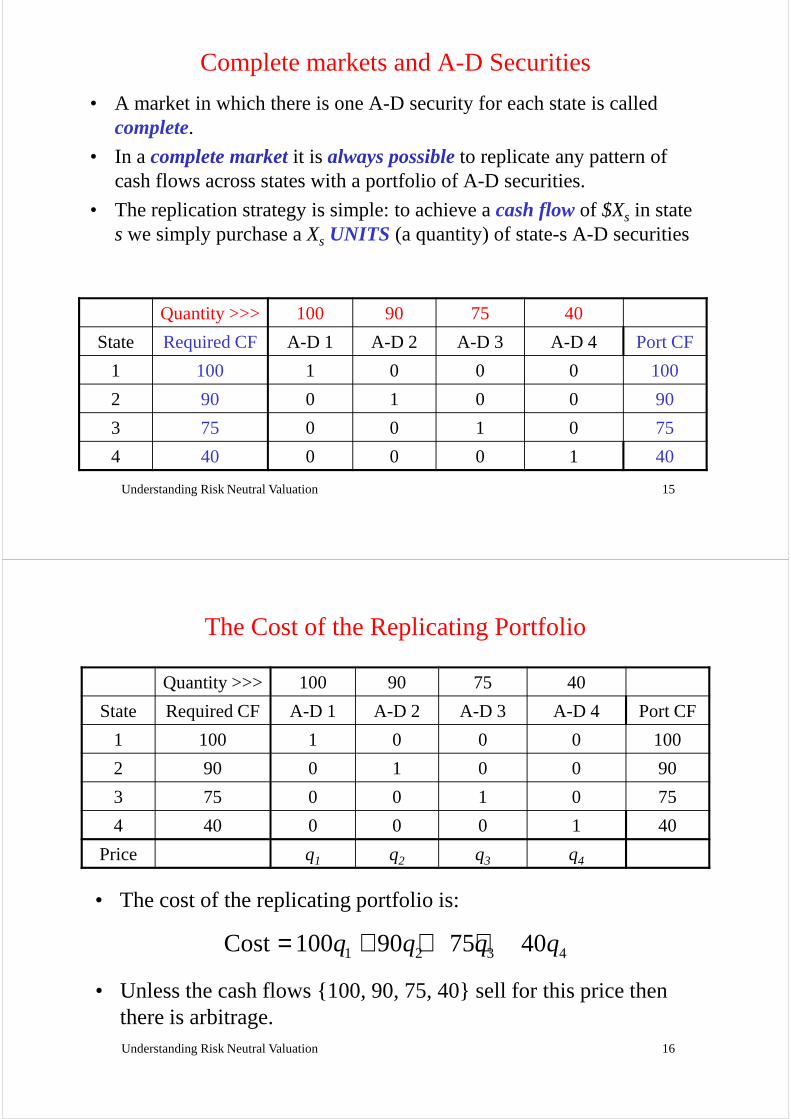
• A market in which there is one A-D security for each state is called complete.
• In a complete marketit is always possible to replicate any pattern of cash flows across states with a portfolio of A-D securities.
• The replication strategy is simple: to achieve a cash flowof $Xs in state s we simply purchase a Xs UNITS (a quantity) of state-s A-D securities
Understanding Risk Neutral Valuation 15
Quantity >>> 100 90 75 40
State Required CF A-D 1 A-D 2 A-D 3 A-D 4 Port CF
1 100 1 0 0 0 100
2 90 0 1 0 0 90
3 75 0 0 1 0 75
4 40 0 0 0 1 40
The Cost of the Replicating Portfolio
Quantity >>> 100 90 75 40
State Required CF A-D 1 A-D 2 A-D 3 A-D 4 Port CF
1 100 1 0 0 0 100
2 90 0 1 0 0 90
3 75 0 0 1 0 75
4 40 0 0 0 1 40
Understanding Risk Neutral Valuation 16
Price q1 q2 q3 q4
• The cost of the replicating portfolio is:
1 2 3 4Cost 100 90 75 40q q q q= + + +
• Unless the cash flows {100, 90, 75, 40} sell for this price then there is arbitrage.
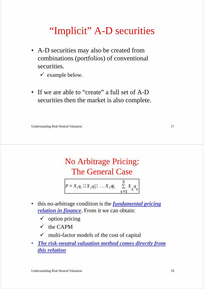
“Implicit” A -D securities
• A-D securities may also be created from combinations (portfolios) of conventional securities. � example below.
Understanding Risk Neutral Valuation 17
� example below.
• If we are able to “create” a full set of A-D securities then the market is also complete.
No Arbitrage Pricing: The General Case
• this no-arbitrage condition is the fundamental pricing relation in finance. From it we can obtain:
� option pricing
1 1 2 2
1S S
SP X q X q X q X q
s ss= + + = ∑
=K
Understanding Risk Neutral Valuation 18
� option pricing
� the CAPM
� multi-factor models of the cost of capital
• The risk-neutral valuation method comes directly from this relation
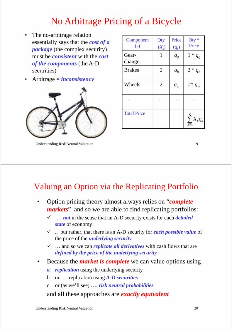
Component (s)
Qty
(Xs)
Price
(qs)
Qty * Price
Gear-change
1 qg 1 * qg
Brakes 2 qb 2 * qb
Wheels 2 q 2* q
No Arbitrage Pricing of a Bicycle• The no-arbitrage relation
essentially says that the cost of a package(the complex security) must be consistentwith the cost of the components(the A-D securities)
• Arbitrage = inconsistency
Understanding Risk Neutral Valuation 19
Wheels 2 qw 2* qw
…. … … …
Total Price
• Arbitrage = inconsistency
1
Ss s
sX q
=∑
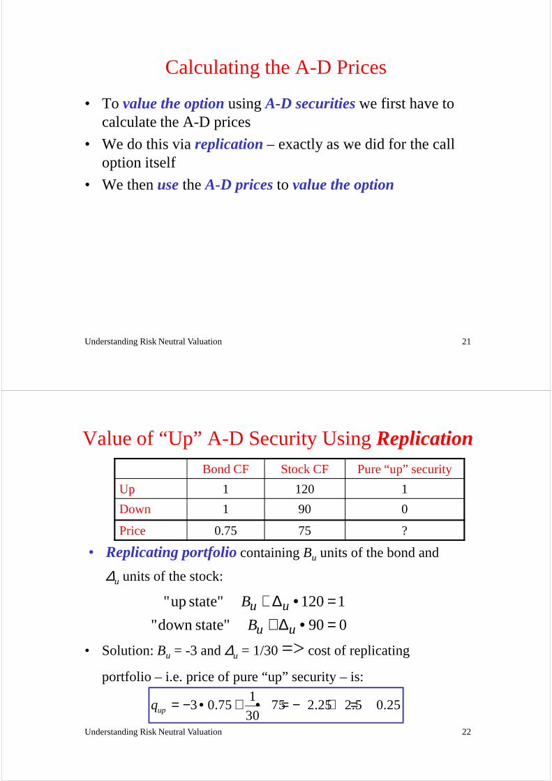
Valuing an Option via the Replicating Portfolio
• Option pricing theory almost always relies on “complete markets” and so we are able to find replicating portfolios:� … not in the sense that an A-D security exists for each detailed
stateof economy
� .. but rather, that there is an A-D security for each possible valueof the price of the underlying security
� … and so we can replicate all derivativeswith cash flows that are
Understanding Risk Neutral Valuation 20
� … and so we can replicate all derivativeswith cash flows that are defined by the price of the underlying security
• Because the market is completewe can value options using a. replicationusing the underlying security
b. or …. replication using A-D securities
c. or (as we’ll see) …. risk neutral probabilities
and all these approaches are exactly equivalent
Calculating the A-D Prices
• To value the optionusing A-D securitieswe first have to calculate the A-D prices
• We do this via replication– exactly as we did for the call option itself
• We then usethe A-D pricesto value the option
Understanding Risk Neutral Valuation 21
Value of “Up” A-D Security Using ReplicationBond CF Stock CF Pure “up” security
Up 1 120 1
Down 1 90 0
Price 0.75 75 ?
• Replicating portfoliocontaining Bu units of the bond and
∆u units of the stock:
Understanding Risk Neutral Valuation 22
090 state"down "
1120 state" up"
=•∆+=•∆+
uu
uu
B
B
• Solution: Bu = -3 and ∆u = 1/30 => cost of replicating
portfolio – i.e. price of pure “up” security – is:1
3 0.75 75 2.25 2.5 0.2530upq = − • + • = − + =
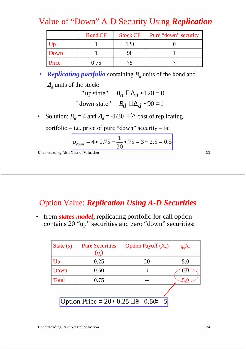
Value of “Down” A-D Security Using Replication
• Replicating portfoliocontaining Bd units of the bond and
∆d units of the stock:
Bond CF Stock CF Pure “down” security
Up 1 120 0
Down 1 90 1
Price 0.75 75 ?
Understanding Risk Neutral Valuation 23
∆d units of the stock:
190 state"down "
0120 state" up"
=•∆+=•∆+
dd
dd
B
B
• Solution: Bd = 4 and ∆d = -1/30 => cost of replicating
portfolio – i.e. price of pure “down” security – is:
14 0.75 75 3 2.5 0.5
30downq = • − • = − =
Option Value: Replication Using A-D Securities
State (s) Pure Securities (qs)
Option Payoff (Xs) qsXs
Up 0.25 20 5.0
• from states model, replicating portfolio for call option contains 20 “up” securities and zero “down” securities:
Understanding Risk Neutral Valuation 24
Up 0.25 20 5.0
Down 0.50 0 0.0
Total 0.75 -- 5.0
Option Price 20 0.25 0 0.50 5= • + • =
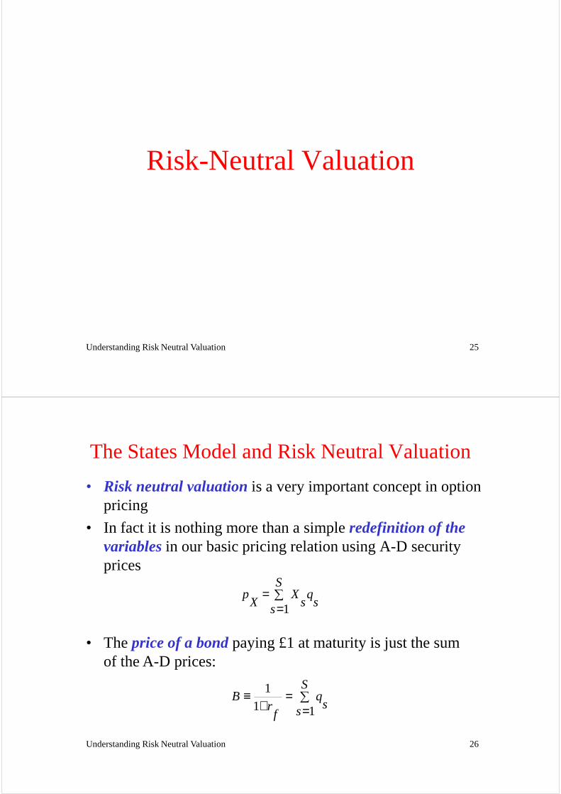
Risk-Neutral Valuation
Understanding Risk Neutral Valuation 25
The States Model and Risk Neutral Valuation
• Risk neutral valuationis a very important concept in option pricing
• In fact it is nothing more than a simple redefinition of the variablesin our basic pricing relation using A-D security prices
Sp X q
X s s= ∑
Understanding Risk Neutral Valuation 26
1p X q
X s ss= ∑
=
• The price of a bondpaying £1 at maturity is just the sum of the A-D prices:
11 1
SB q
sr sf
≡ = ∑+ =
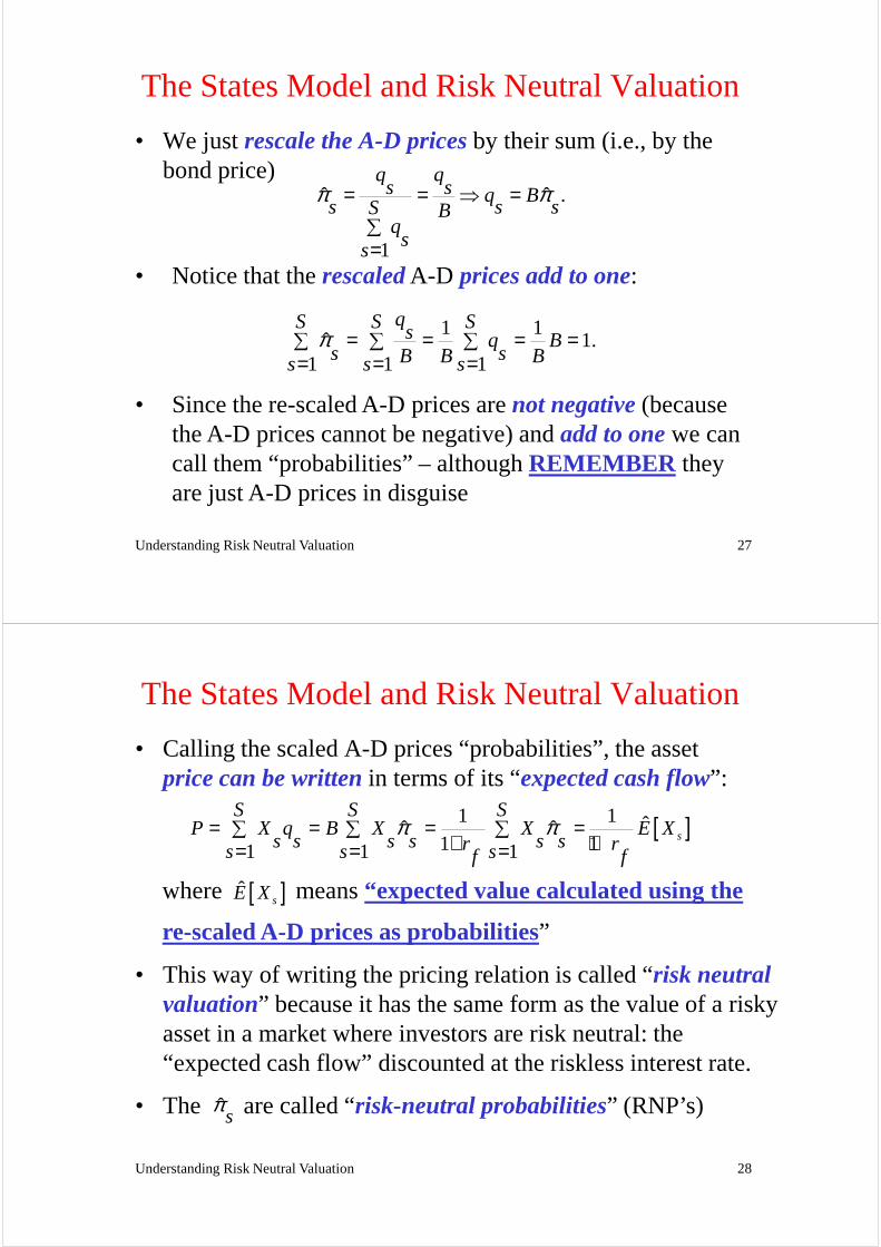
The States Model and Risk Neutral Valuation
• We just rescale the A-D pricesby their sum (i.e., by the bond price)
.ˆ ˆ
1
q qs s q B
s s sS Bq
ss
π π= = ⇒ =∑=
• Notice that the rescaledA-D prices add to one:
qS S S
Understanding Risk Neutral Valuation 27
1 11.ˆ
1 1 1
qS S Ss q Bs sB B Bs s s
π = = = =∑ ∑ ∑= = =
• Since the re-scaled A-D prices are not negative(because the A-D prices cannot be negative) andadd to onewe can call them “probabilities” – although REMEMBER they are just A-D prices in disguise
The States Model and Risk Neutral Valuation
• Calling the scaled A-D prices “probabilities”, the asset price can be writtenin terms of its “expected cash flow”:
[ ]1 1 ˆˆ ˆ1 11 1 1
s
S S SP X q B X X E X
s s s s s sr rs s sf f
π π= = = =∑ ∑ ∑+ += = =
where means “expected value calculated using the
re-scaled A-D prices as probabilities”
[ ]ˆsE X
Understanding Risk Neutral Valuation 28
re-scaled A-D prices as probabilities”
• This way of writing the pricing relation is called “risk neutral valuation” because it has the same form as the value of a risky asset in a market where investors are risk neutral: the “expected cash flow” discounted at the riskless interest rate.
• The are called “risk-neutral probabilities” (RNP’s)ˆs
π
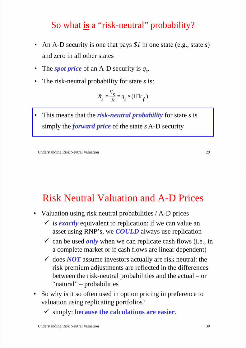
So what is a “risk-neutral” probability?
• An A-D security is one that pays $1 in one state (e.g., state s)
and zero in all other states
• The spot priceof an A-D security is qs.
• The risk-neutral probability for state s is:
Understanding Risk Neutral Valuation 29
(1 )ˆq
s q rs s fB
π = = × +
• This means that the risk-neutral probability for state s is
simply the forward priceof the state s A-D security
Risk Neutral Valuation and A-D Prices• Valuation using risk neutral probabilities / A-D prices
� is exactlyequivalent to replication: if we can value an asset using RNP’s, we COULD always use replication
� can be used only when we can replicate cash flows (i.e., in a complete market or if cash flows are linear dependent)
� does NOT assume investors actually are risk neutral: the
Understanding Risk Neutral Valuation 30
� does NOT assume investors actually are risk neutral: the risk premium adjustments are reflected in the differences between the risk-neutral probabilities and the actual – or “natural” – probabilities
• So why is it so often used in option pricing in preference to valuation using replicating portfolios?
� simply: because the calculations are easier.
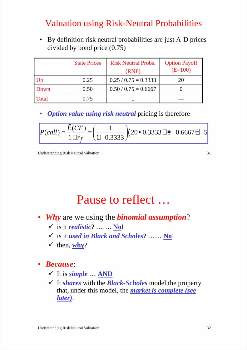
Valuation using Risk-Neutral Probabilities
• By definition risk neutral probabilities are just A-D prices divided by bond price (0.75)
State Prices Risk Neutral Probs.
(RNP)
Option Payoff (E=100)
Up 0.25 0.25 / 0.75 = 0.3333 20
Down 0.50 0.50 / 0.75 = 0.6667 0
Understanding Risk Neutral Valuation 31
Down 0.50 0.50 / 0.75 = 0.6667 0
Total 0.75 1 ---
• Option value using risk neutralpricing is therefore
( )ˆ ( ) 1
( ) 20 0.3333 0 0.6667 51 1 0.3333f
E CFP call
r = = • + • = + +
Pause to reflect …• Whyare we using the binomial assumption?
� is it realistic? ……. No!� is it used in Black and Scholes? …… No!� then, why?
• Because:
Understanding Risk Neutral Valuation 32
• Because:� It is simple… AND� It shareswith the Black-Scholesmodel the property
that, under this model, the market is complete (see later).
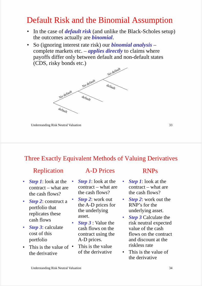
Default Risk and the Binomial Assumption• In the case of default risk (and unlike the Black-Scholes setup)
the outcomes actually are binomial.• So (ignoring interest rate risk) our binomial analysis –
complete markets etc. –applies directly to claims where payoffs differ only between default and non-default states (CDS, risky bonds etc.)
Understanding Risk Neutral Valuation 33
Three Exactly Equivalent Methods of Valuing Derivatives
• Step 1: look at the contract – what are the cash flows?
• Step 2: construct a portfolio that replicates these
• Step 1: look at the contract – what are the cash flows?
• Step 2: work out the A-D prices for the underlying asset.
Replication A-D Prices
• Step 1: look at the contract – what are the cash flows?
• Step 2: work out the RNP’s for the underlying asset.Step 3
RNPs
Understanding Risk Neutral Valuation 34
replicates these cash flows
• Step 3: calculate cost of this portfolio
• This is the value of the derivative
asset.• Step 3: Value the
cash flows on the contract using the A-D prices.
• This is the value of the derivative
• Step 3Calculate the risk neutral expected value of the cash flows on the contract and discount at the riskless rate
• This is the value of the derivative
Why Risk Neutral Valuation can be easier than Replication
Understanding Risk Neutral Valuation 35
be easier than Replication
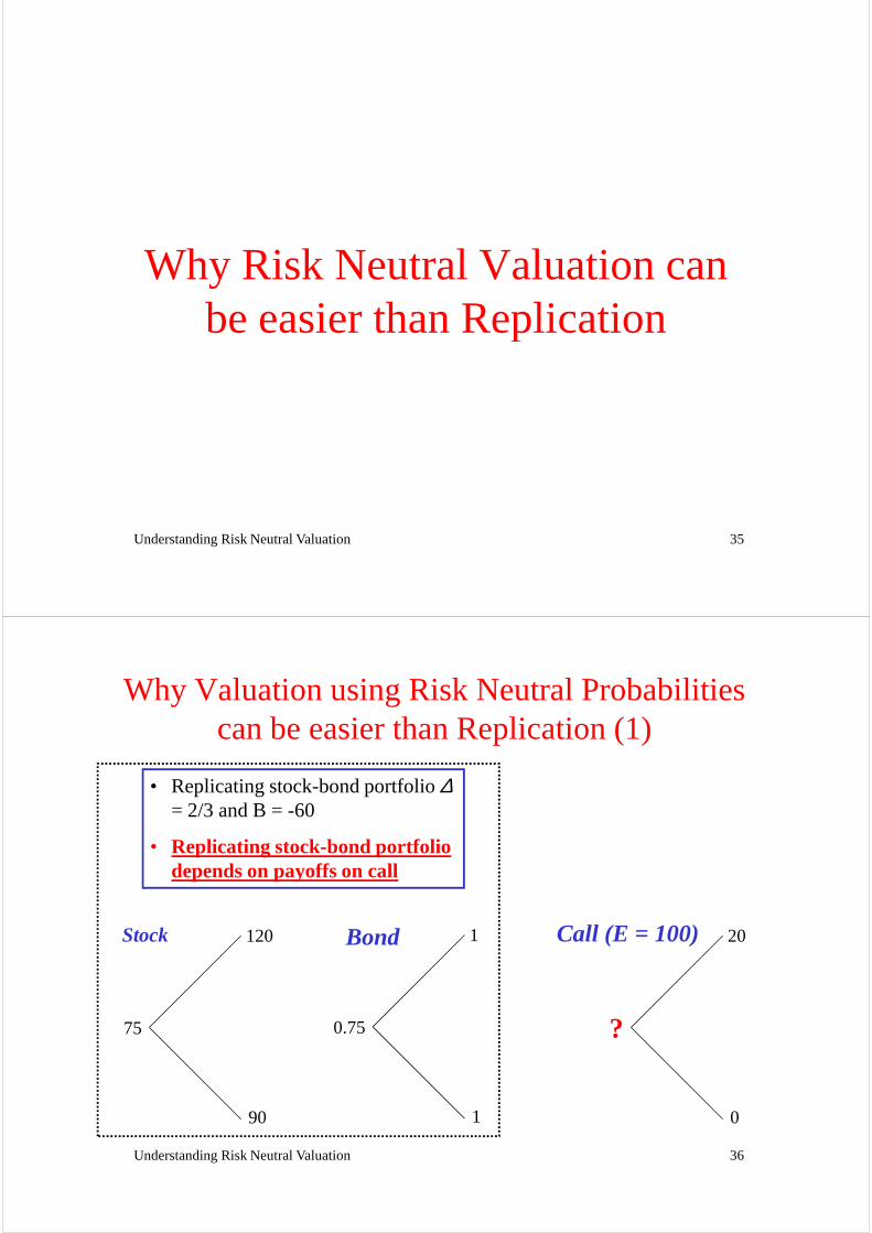
Why Valuation using Risk Neutral Probabilities can be easier than Replication (1)
Stock Bond Call (E = 100)
• Replicating stock-bond portfolio ∆= 2/3 and B = -60
• Replicating stock-bond portfolio depends on payoffs on call
Understanding Risk Neutral Valuation 36
120
90
75
Stock 1
1
0.75
Bond 20
0
?
Call (E = 100)
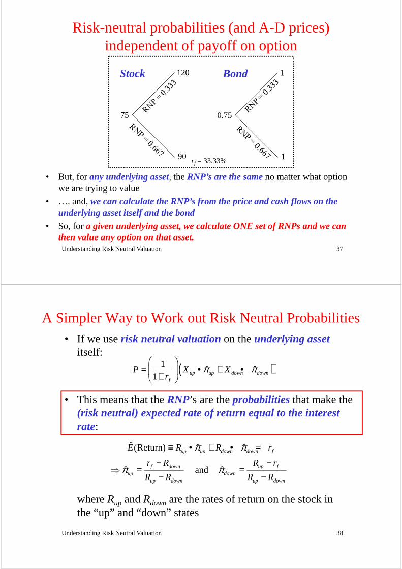
Risk-neutral probabilities (and A-D prices) independent of payoff on option
120
75
Stock 1
0.75
Bond
Understanding Risk Neutral Valuation 37
90 1
• But, for any underlying asset, the RNP’s are the sameno matter what option we are trying to value
• …. and, we can calculate the RNP’s from the price and cash flows on the underlying asset itself and the bond
• So, for a given underlying asset, we calculate ONE set of RNPs and we can then value any option on that asset.
rf = 33.33%
A Simpler Way to Work out Risk Neutral Probabilities• If we use risk neutral valuationon the underlying asset
itself:
( )1ˆ ˆ
1 up up down downf
P X Xr
π π
= • + • +
• This means that the RNP’s are the probabilitiesthat make the (risk neutral) expected rate of return equal to the interest rate:
Understanding Risk Neutral Valuation 38
ˆ (Return) ˆ ˆ
and ˆ ˆ
up up down down f
f down up fup down
up down up down
E R R r
r R R r
R R R R
π π
π π
≡ • + • =
− −⇒ = =
− −
rate:
where Rup and Rdown are the rates of return on the stock in the “up” and “down” states
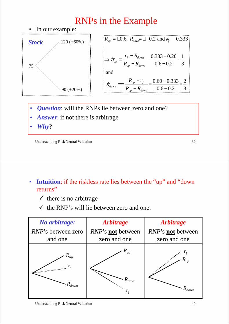
RNPs in the Example• In our example:
0.6, 0.2 and 0.333
0.333 0.20 1= =ˆ
0.6 0.2 3
and
0.60 0.333 2
up down f
f downup
up down
up f
R R r
r R
R R
R r
π
π
= + = + =
− −⇒ =
− −
− −==
120 (+60%)
75
Stock
Understanding Risk Neutral Valuation 39
0.60 0.333 2 = = ˆ
0.6 0.2 3up f
downup down
R r
R Rπ
− −==− −
• Question: will the RNPs lie between zero and one?
• Answer: if not there is arbitrage
• Why?
90 (+20%)
• Intuition : if the riskless rate lies between the “up” and “down returns”
� there is no arbitrage
� the RNP’s will lie between zero and one.
No arbitrage:
RNP’s between zero and one
Arbitrage
RNP’s not between zero and one
Arbitrage
RNP’s not between zero and one
Understanding Risk Neutral Valuation 40
Rup
rf
Rdown
Rup
rf
Rdown
Rup
rf
Rdown
Market Completeness and Trading
Understanding Risk Neutral Valuation 41
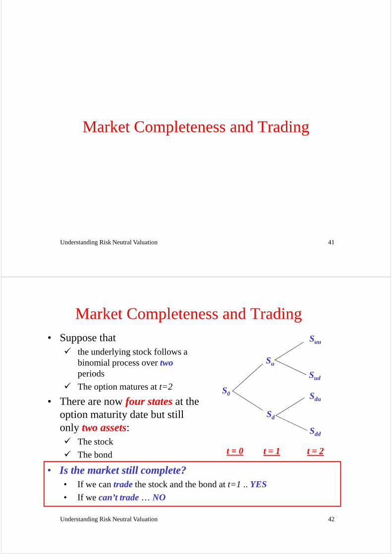
Market Completeness and Trading• Suppose that
� the underlying stock follows a binomial process over twoperiods
� The option matures at t=2
• There are now four statesat the option maturity date but still Sd
Suu
Sud
Sdu
Su
S0
Understanding Risk Neutral Valuation 42
option maturity date but still only two assets:� The stock
� The bond
Sd
Sdd
t = 2t = 1t = 0
• Is the market still complete?• If we can tradethe stock and the bond at t=1 .. YES
• If we can’t trade… NO
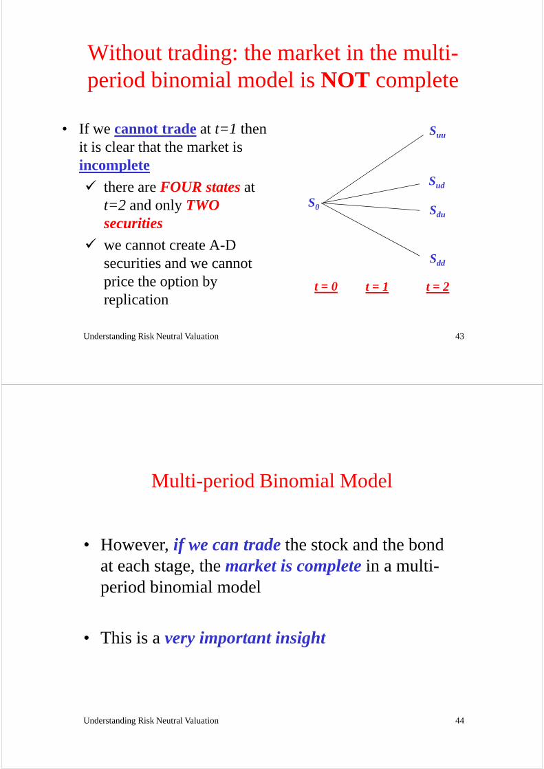
Without trading: the market in the multi-period binomial model is NOT complete
• If we cannot tradeat t=1 then it is clear that the market is incomplete� there are FOUR statesat
Suu
Sud
Understanding Risk Neutral Valuation 43
� there are FOUR statesat t=2 and only TWO securities
� we cannot create A-D securities and we cannot price the option by replication
Sdd
Sdu
t = 2t = 1t = 0
S0
Multi-period Binomial Model
• However, if we can tradethe stock and the bond at each stage, the market is completein a multi-
Understanding Risk Neutral Valuation 44
period binomial model
• This is a very important insight
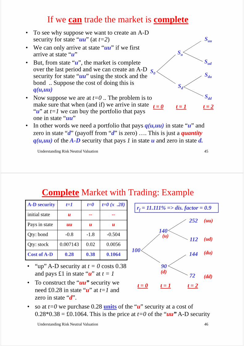
If we can trade the market is complete• To see why suppose we want to create an A-D
security for state “uu” (at t=2)• We can only arrive at state “uu” if we first
arrive at state “u” • But, from state “u”, the market is complete
over the last period and we can create an A-D security for state “uu” using the stock and the bond .. Suppose the cost of doing this is q(u,uu)
Sd
Suu
Sud
Sdu
Su
S0
Understanding Risk Neutral Valuation 45
q(u,uu)• Now suppose we are at t=0 .. The problem is to
make sure that when (and if) we arrive in state “u” at t=1 we can buy the portfolio that pays one in state “uu”
Sd
Sdd
t = 2t = 1t = 0
• In other words we need a portfolio that pays q(u,uu) in state “u” and zero in state “d” (payoff from “d” is zero) …. This is just a quantityq(u,uu) of theA-D security that pays 1 in state u and zero in state d.
CompleteMarket with Trading: Example
100
140
r f = 11.111% => dis. factor = 0.9
144
112
252
(u)
(uu)
(ud)
(du)
A-D security t=1 t=0 t=0 (x .28)
initial state u -- --
Pays in state uu u u
Qty: bond -0.8 -1.8 -0.504
Qty: stock 0.007143 0.02 0.0056
Cost of A-D 0.28 0.38 0.1064
Understanding Risk Neutral Valuation 46
t = 2t = 1t = 0
90
72 (dd)(d)
• so at t=0 we purchase 0.28 units of the “u” security at a cost of 0.28*0.38 = £0.1064. This is the price at t=0 of the “uu” A-D security
• “up” A-D security at t = 0 costs 0.38 and pays £1 in state “u” at t = 1
• To construct the “uu” security we need £0.28 in state “u” at t=1 and zero in state “d”.
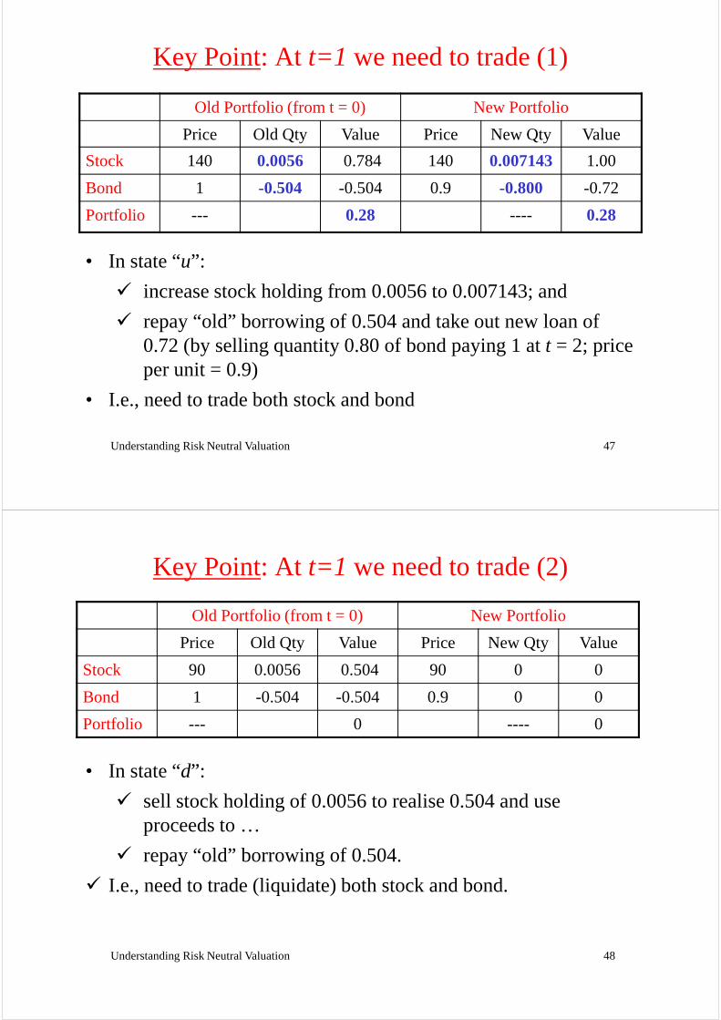
Key Point: At t=1 we need to trade (1)
Old Portfolio (from t = 0) New Portfolio
Price Old Qty Value Price New Qty Value
Stock 140 0.0056 0.784 140 0.007143 1.00
Bond 1 -0.504 -0.504 0.9 -0.800 -0.72
Portfolio --- 0.28 ---- 0.28
• In state “u”:
Understanding Risk Neutral Valuation 47
• In state “u”:
� increase stock holding from 0.0056 to 0.007143; and
� repay “old” borrowing of 0.504 and take out new loan of 0.72 (by selling quantity 0.80 of bond paying 1 at t = 2; price per unit = 0.9)
• I.e., need to trade both stock and bond
Key Point: At t=1 we need to trade (2)
Old Portfolio (from t = 0) New Portfolio
Price Old Qty Value Price New Qty Value
Stock 90 0.0056 0.504 90 0 0
Bond 1 -0.504 -0.504 0.9 0 0
Portfolio --- 0 ---- 0
• In state “d”:
Understanding Risk Neutral Valuation 48
• In state “d”:
� sell stock holding of 0.0056 to realise 0.504 and use proceeds to …
� repay “old” borrowing of 0.504.
� I.e., need to trade (liquidate) both stock and bond.
CompleteMarket with Trading: Example, contd.
• Example shows that when we can trade a long-lived security (e.g., a stock) a market may be complete even though the number of securities is smaller than the number of states� notice that we had to trade the stock and the bond at time t = 1 (we
increase stock holding from 0.0056 to 0.007143 and borrow more)
• This insight is key to understanding the Black-Scholes model in which:� there are just two assets:the stock and the bond. (apart from options)
Understanding Risk Neutral Valuation 49
� there are just two assets:the stock and the bond. (apart from options)� there is an infinite number of states� but … the market is nonetheless complete
• Example on previous slide is important but replication is usually a complicated way to do the calculations
• For multi-period options generally easier to use the risk-neutral approach and work out the RNPs from the “up” and “down” rates of return on the stock and the interest rate
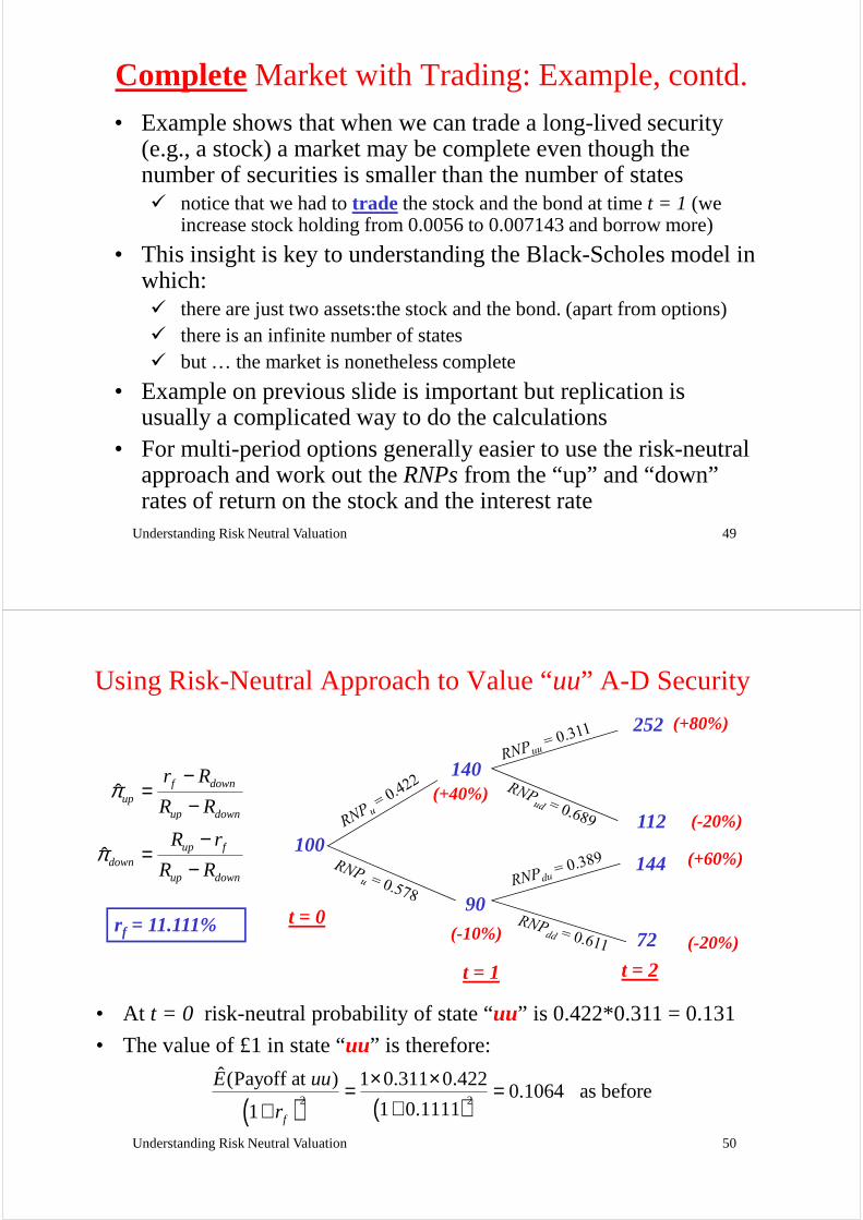
Using Risk-Neutral Approach to Value “uu” A-D Security
ˆ
ˆ
f downup
up down
up fdown
up down
r R
R R
R r
R R
π
π
−=
−
−=
−
t = 0
100
140
90r = 11.111%
144
112
252
(+40%)
(-20%)
(+60%)
(+80%)
Understanding Risk Neutral Valuation 50
t = 2t = 1
t = 090
r f = 11.111% 72 (-20%)(-10%)
• At t = 0 risk-neutral probability of state “uu” is 0.422*0.311 = 0.131
• The value of £1 in state “uu” is therefore:
( ) ( )2 2
ˆ (Payoff at ) 1 0.311 0.4220.1064 as before
1 0.11111 f
E uu
r
× ×= =++
A last word on completeness
• Notice that nothing about completeness depends on the probability of different states .. only on the number of possiblestates
• We have seen that when we can trade the underlying asset we can have complete set of A-D securities for some future date even when the number of securities is much smaller
Understanding Risk Neutral Valuation 51
date even when the number of securities is much smaller than the number of states
• However, in the discrete time case (i.e., not in the Black-Scholes framework) completeness requires that over any period when we can’t trade (e.g., betweent=0 and t=1) the number of securities IS at least as large as the number of states
Key Concepts
• A-D securities
• market completeness
• valuing options using � replication
� A-D prices
• relation between trading and market completeness in multi-period binomial case
• valuing options using risk neutral probabilities in
Understanding Risk Neutral Valuation 52
� A-D prices
� risk neutral probabilities
• calculating risk-neutral probabilities from “up” and “down” returns on stock
neutral probabilities in multi-period trees
• valuing American options in multi-period trees