UNDERSTANDING SEWER INFILTRATION AND INFLOW USING …

UNDERSTANDING SEWER INFILTRATION AND INFLOW

USING IMPULSE RESPONSE FUNCTIONS

DERIVED FROM PHYSICS-BASED MODELS

BY

NAM JEONG CHOI

DISSERTATION

Submitted in partial fulfillment of the requirements

for the degree of Doctor of Philosophy in Civil Engineering

in the Graduate College of the

University of Illinois at Urbana-Champaign, 2016

Urbana, Illinois

Doctoral Committee:

Professor Albert J Valocchi, Chair

Research Assistant Professor Arthur R Schmidt, Director of Research

Professor Marcelo H Garcia

Associate Professor Richard A Cooke

Doctor Joshua Cantone (Wallbridge & Gilbert, University of Adelaide)

ii

Abstract

Infiltration and inflow (I&I) are extraneous flow in a sanitary sewer system that originate from

surface water and ground water. I&I can overload the sewer system and wastewater treatment

plants, and cause sanitary sewer overflows (SSOs) or basement flooding. This flow can account

for as much as ten times dry weather flow (DWF) but the estimation of the volume and peak of

I&I involves a great deal of uncertainty.

Temporal and spatial variability of the I&I processes make it difficult to understand the

phenomena. Depending on the time scale of different I&I processes, some watershed properties

may only affect specific I&I sources. For example, the configuration of sewer network and the

geology of the watershed may affect fast and slow I&I processes differently.

In this study, the physical process of three major I&I sources: roof downspout, sump pump, and

leaky lateral, are investigated at the residential lot scale using physics-based models. The typical

flow response of each I&I source is calculated and these flow responses, called Impulse

Response Functions (IRFs), are evaluated. I&I estimation using the three IRFs, calibrated using a

genetic algorithm (GA), was performed on a catchment in the Chicago area at the sewershed

scale. Results are compared with one of the most widely used I&I estimation methods, the RTK

method. The IRF method shows more stable solutions as the model is based on physical

processes. The RTK method better predicts the monitoring data, however it is suspected that this

is mainly because the RTK method is an empirical curve fitting method.

Uncertainty related to rainfall induced infiltration (RII) is further investigated on six different

input parameters: Antecedent moisture condition (AMC), pedotransfer functions (PTFs), soil

hydraulic conductivities, initial conditions (IC), sewer pipe depths, and rainfall characteristics.

iii

The uncertainty analysis indicates that the model result is most sensitive to the soil hydraulic

conductivity, which defines the maximum infiltration rate. Rainfall characteristics, including

duration and hyetograph shape turn out to be the least influential factors affecting the infiltration

response.

Results from this study help understand the sewer I&I process in a complex urban system. In

particular, using a small scale, detailed distributed model enables examination of the sensitivity

of the I&I process to the different factors contributing to uncertainty. While the modeling results

are site specific to Hickory Hills, IL, this study can provide insights to researchers and engineers

about characteristic behaviors of different I&I sources and the uncertainty factors that affect

sewer infiltration response including AMC.

iv

Table of Contents

List of Figures ................................................................................................................................ vi

List of Tables ................................................................................................................................. ix

1. Introduction ............................................................................................................................. 1

1.1. Research Background and Motivation ................................................................................. 1

1.2. Research Objectives ........................................................................................................... 10

References ................................................................................................................................. 12

2. Literature Review .................................................................................................................. 18

2.1. Definition and Sources of I&I ............................................................................................ 18

2.2. Methods to Estimate I&I .................................................................................................... 21

2.3. Space and Time Variability of I&I Process ....................................................................... 24

References ................................................................................................................................. 26

3. Methodology .......................................................................................................................... 33

3.1. Introduction ........................................................................................................................ 33

3.2. Space and Time Scale of I&I Processes ............................................................................. 36

3.3. Modeling of I&I Response Functions ................................................................................ 42

3.4. Genetic Algorithm for Model Calibration .......................................................................... 55

References ................................................................................................................................. 61

4. I&I Response Functions ........................................................................................................ 69

4.1. Typical I&I Response Functions ........................................................................................ 69

4.2. Model Calibration .............................................................................................................. 76

References ................................................................................................................................. 96

5. Uncertainty in Rainfall Induced Infiltration .......................................................................... 97

5.1. Introduction ........................................................................................................................ 97

5.2. Uncertainty Factors .......................................................................................................... 102

v

5.3. Results and Discussion ..................................................................................................... 113

5.4. Summary .......................................................................................................................... 123

References ............................................................................................................................... 125

Summary and Conclusions ......................................................................................................... 129

Future Research and Suggestions ............................................................................................... 133

vi

List of Figures

Figure 1.1 Three parameters: R, T, and K of the RTK method illustrated with one of three RTK

hydrographs .......................................................................................................................... 5

Figure 1.2 InfoWorks CS infiltration module ................................................................................. 6

Figure 2.1 Root intrusion through cracks and joints of sewer pipes (Images from Urbana

Champaign Sanitary District 2012) .................................................................................... 20

Figure 3.1 Hydrological processes at a range of characteristic space-time scales (Blöschl &

Sivapalan 1995) .................................................................................................................. 37

Figure 3.2 Random I&I and DWF input locations in a sewer system .......................................... 39

Figure 3.3 Effect of random locations of I&I sources in a sewer network on the fast and slow I&I

............................................................................................................................................ 40

Figure 3.4 Three random I&I locations and the distance to the outlet in the least efficient

drainage network (a) and the most efficient network (original source of the networks from

Seo 2012) ............................................................................................................................ 41

Figure 3.5 Roof connection model domain................................................................................... 43

Figure 3.6 Typical foundation drain and sump pump features in a home construction with a sump

pump flow in a solid line and a gravity flow in a dashed line; all drain to day light or

sewer (modified from Depew 1992) .................................................................................. 49

Figure 3.7 Soil profile definitions of the sump pump modeling (a) plan view (b) vertical view

(figures not drawn to scale) ................................................................................................ 50

Figure 3.8 Soil profile definitions of the leaky lateral modeling (a) plan view (b) vertical view

(figures not drawn to scale) ................................................................................................ 54

Figure 3.9 Conceptual I&I impulse response functions (IRF) for (a) roof connection, (b) sump

pump, and (c) leaky lateral with five consecutive impulse rainfall (refer to equation (2) for

index) .................................................................................................................................. 55

Figure 3.10 Convolution of I&I responses and DWF using SWMM for (a) IRF method (b) RTK

method (not scaled proportionally) .................................................................................... 57

Figure 3.11 An example of crossover and mutation process ........................................................ 59

Figure 4.1 Simplified representative rainfall with the maximum rainfall peak 14 mm/hr ........... 70

Figure 4.2 Flow responses from roof connection, sump pump, and leaky lateral models with 42

mm uniform rainfall (a) overall responses, (b) zoomed in view of roof runoff and sump

pump flow........................................................................................................................... 71

Figure 4.3 Flow responses from roof drain, sump pump, and leaky lateral models with real

rainfall data (a) rainfall, (b) overall flow responses, (c) zoomed in view of the period from

June 16, 2009 to July 3, 2009 ............................................................................................. 74

Figure 4.4 Exceedance probability of three I&I responses: Roof connection, sump pump

connection, and leaky lateral, per unit area from April 17 to July 16, 2009 (in log scale) 76

Figure 4.5 Sewage monitoring locations including the test site 17 in the monitoring area Hickory

Hills, Palos Hills, and Bridgeview, IL (Black solid line with dots indicates main trunk

vii

sewer, arrow line indicates local sewer entry, dashed lines indicate street reference marks)

............................................................................................................................................ 77

Figure 4.6 Rainfall and sewer flow data (a) rainfall record from ISWS (b) flow data from USGS

sewage monitoring site 17 .................................................................................................. 78

Figure 4.7 Daily and hourly patterns of DWF .............................................................................. 80

Figure 4.8 Sensitivity tests on IRF parameters (R; roof connection coefficient, S; sump pump

connection coefficient, and L; leaky lateral coefficient) and Nash-Sutcliffe coefficients

with (a) different probability of crossover values (with probability of mutation 0.06), and

(b) different probability of mutation values (with probability of cross over 0.93) ............ 83

Figure 4.9 Box plots of RTK solutions in Table 4.5 ..................................................................... 88

Figure 4.10 Three RTK triangular hydrographs from 30 different model runs (flowrate for 1 cm

of rain over the unit area 1 km2) ......................................................................................... 88

Figure 4.11 Case 15 and case 16 of RTK parameter solutions in Table 4.5 that result in similar

Nash-Sutcliffe model fitness coefficients: 0.797 and 0.794, respectively (flowrate for 1 cm

of rain over the unit area 1 km2) ......................................................................................... 88

Figure 4.12 IRF-GA and RTK-GA results in the (a) calibration period (May 9, 2009 to June 7,

2009) and the (b) validation period (June 9, 2009 to July 8, 2009) ................................... 89

Figure 4.13 Comparison of the best cases of IRF and RTK solutions for four different periods . 91

Figure 4.14 Residual plots of IRF and RTK methods for (a) calibration period and (b) validation

period .................................................................................................................................. 93

Figure 5.1 Sources of uncertainties (modified from Figure 1.1 in Tung & Yen (2005)) ........... 100

Figure 5.2 Changed hyetographs with the addition of 3-hr 42-mm uniform rainfall at ten random

times listed in Table 1 of chapter 4 .................................................................................. 103

Figure 5.3 Infiltration response for the rainfall perturbation derived by subtracting the response

from the rainfall without the perturbation using the July 28th, 2009 case (average of this

response for ten different cases become leaky lateral IRF) .............................................. 104

Figure 5.4 Sewer junctions in Hickory Hills, IL with elevation data availability ...................... 109

Figure 5.5 Sewer junction depths distribution in Hickory Hills, IL ........................................... 110

Figure 5.6 Tested rainfall durations and shapes (representative case with 3-hour 42-mm rainfall)

.......................................................................................................................................... 112

Figure 5.7 Arbitrary inclusion of the rainfall perturbation using the representative case .......... 112

Figure 5.8 Infiltration flow response with three distinguishable AMCs (a) forward response with

average infiltration volume 47 mm, (b) centered response with average infiltration volume

45 mm, (c) backward response with average infiltration volume 44 mm, (d) average

cumulative rainfall depths for forward, centered, and backward cases ............................ 114

Figure 5.9 Hydraulic conductivity values of different soil types in Hickory Hills, IL using

different PTFs along with average hydraulic conductivity; a thin solid line indicates one

soil type, the thick solid line with black cross markers indicates the arithmetic mean and

thick solid line with square markers indicates the area weighted mean) ......................... 115

viii

Figure 5.10 Model input and results of different soil hydraulic conductivity tests (a) rainfall

input, (b) infiltration rate at the leaky lateral with different hydraulic conductivity values

as unsaturated flow, (c) maximum peak values, and (d) elapsed time to the onset of flow

response compare to the largest Ks case (Ks = 1.80·10-6 m/s) .......................................... 117

Figure 5.11 Infiltration hydrographs with different sewer pipe depths; peak investigation (a)

Infiltration hydrographs, (b) Peak magnitudes, (c) Peak time (Square markers indicate the

beginning of each infiltration response, circle markers indicate peak 1, and rhombus

markers indicate peak 2) ................................................................................................... 118

Figure 5.12 Infiltration hydrographs with different sewer pipe depths; tail investigation (a)

Infiltration hydrographs, (b) Tail magnitude, (c) Delay time (Square markers indicate the

beginning of each infiltration response, circle markers indicate tail 1, and rhombus

markers indicate tail2) ...................................................................................................... 120

Figure 5.13 Comparison of infiltration response for the converged case and the test case of

March 3rd, 2009 ................................................................................................................ 121

Figure 5.14 Percent error in infiltration rate of the nine test cases with different starting times (a)

Individual error curves, (b) Median and average along with the maximum, minimum, 1st

quartile, and 3rd quartile values ....................................................................................... 122

Figure 5.15 Flow responses from different rainfall durations and shapes .................................. 123

ix

List of Tables

Table 1.1 Amount of I&I relative to DWF from different sources of literature ............................. 3

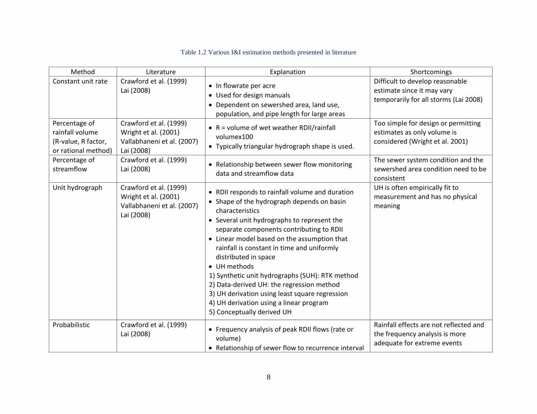
Table 1.2 Various I&I estimation methods presented in literature ................................................. 8

Table 1.3 Summary of the agricultural drainage literature related to modeling ............................. 9

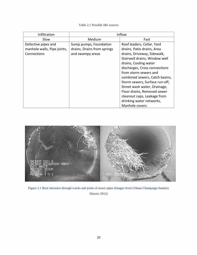
Table 2.1 Possible I&I sources ..................................................................................................... 20

Table 2.2 Sewer inspection and rehabilitation techniques in 1960’s and 1970’s ......................... 23

Table 3.1 Distance of three I&I sources to the outlet ................................................................... 42

Table 4.1 Randomly selected times to insert 42 mm uniform rainfall to define typical I&I

responses .............................................................................................................................. 70

Table 4.2 DWF patterns at sewage monitoring site 17 ................................................................. 79

Table 4.3 Contributing flow volume of three I&I sources using the IRF volume and the

weighting coefficients .......................................................................................................... 84

Table 4.4 IRF-GA and RKT-GA results with Nash-Sutcliffe coefficients for the calibration

period (May 9, 2009 to June 7, 2009) and validation period (June 9, 2009 to July 8, 2009)

.............................................................................................................................................. 86

Table 4.5 Parameter boundary values and solutions of 30 random RTK-GA runs along with

Nash-Sutcliffe coefficients for the calibration period (May 9, 2009 to June 7, 2009) ........ 87

Table 4.6 Volume and peak of the estimated DWF, observed sewer flow, IRF result, and RTK

result for five storm events (Flowrate over 0.3 cms is used as the criteria to separate storms

and following formula is used to compare. (Compare to DWF) = (Observed sewer

flow)/(Estimated DWF), (Compare to monitoring) = ((IRF or RTK)-(Observed sewer

flow))/( Observed sewer flow)*100, Negative values are in italic.) .................................... 92

Table 4.7 Improved model fitness using a weighted Nash-Sutcliffe method in the IRF-GA and

RKT-GA for the calibration period (May 9, 2009 to June 7, 2009) and validation period

(June 9, 2009 to July 8, 2009) (R = Roof connection scaling factor, S = Sump pump

connection scaling factor, L = Leakey sewer lateral scaling factor) .................................... 95

Table 5.1 Uncertainty involved in six factors of interest ............................................................ 101

Table 5.2 Hydraulic conductivity values for the test .................................................................. 108

Table 5.3 Tested sewer depths .................................................................................................... 110

Table 5.4 Test cases with different simulation start times to investigate the initial condition (IC)

............................................................................................................................................ 111

Table 5.5 Average hydraulic conductivity values (arithmetic mean and area weighted mean)

estimated by different PTFs and the comparison of the area weighted mean to the average

hydraulic conductivity from the data ................................................................................. 116

1

1. Introduction

1.1. Research Background and Motivation

Capital investment needs for fixing and expanding sewer pipes in the US are estimated to exceed

$200 billion over the next twenty years, which is three quarters of entire investment requirement

in wastewater system (USEPA 2013). Between 700,000 and 800,000 miles of public sewer

mains in the states are reaching the end of their useful life and 900 billion gallons of sanitary

sewer overflows and combined sewer overflows are estimated each year (ASCE 2013). One of

the biggest problems related to sewer system maintenance is infiltration and inflow (I&I) that

causes sewer overflows and basement flooding. Thus, continuous maintenance of the system

along with understanding the characteristics of the factors causing sewer problems is necessary.

I&I is recognized as one of the major problems affecting sewer systems and results in associated

problems such as (Field & Struzeski 1972, NSFC 1999, Lai 2008):

Flow overloading in sewer systems and water treatment plants and associated problems

e.g. street flooding, basement flooding (Gottstein 1976)

Increase in pumping costs (Backmeyer 1960)

Sewer overflows and associated adverse effects of pollution and public health

Decrease in treatment efficiency in water treatment plants caused by dilution

The excessive I&I flow can cause flow overloading in sewer systems and may result in basement

flooding during periods of intensive rainfall (Gottstein 1976). In sewer systems with a large

2

number of pumping stations (e.g. Florida) pumping costs could be also substantial as the

wastewater volume increases (Backmeyer 1960). Sewer overflow is strongly regulated by the

EPA and failure to remove overflows or to correct I&I problems could prevent a city from

receiving federal construction grant funds (Sliter 1974). Overflows and bypasses of sewage

degrade receiving water quality and may cost the community a violation fee that is forced by

state and federal laws. Bypassed raw sewage may also cause odor problems and adverse impacts

on public health. In coastal areas, infiltration of salt water can deteriorate sewer pipes and water

treatment plant facilities by providing an extra source of sulfur (Backmeyer 1960). Wastewater

treatment and collection systems account for 10 to 15 percent of the total infrastructure values in

the US (NCPWI 1988) and I&I problems need to be addressed with a great emphasis.

Based on Petroff (1996)’s estimation, around 50% of the treated wastewater in the US is from

rainfall-derived I&I (RDII) and dry weather infiltration. Franz (2007) also highlighted that 20%

of the waste water treated in Germany is extraneous water. The amount of I&I varies in different

sewer systems depending on the age of the system, pipe material, construction practices, soil

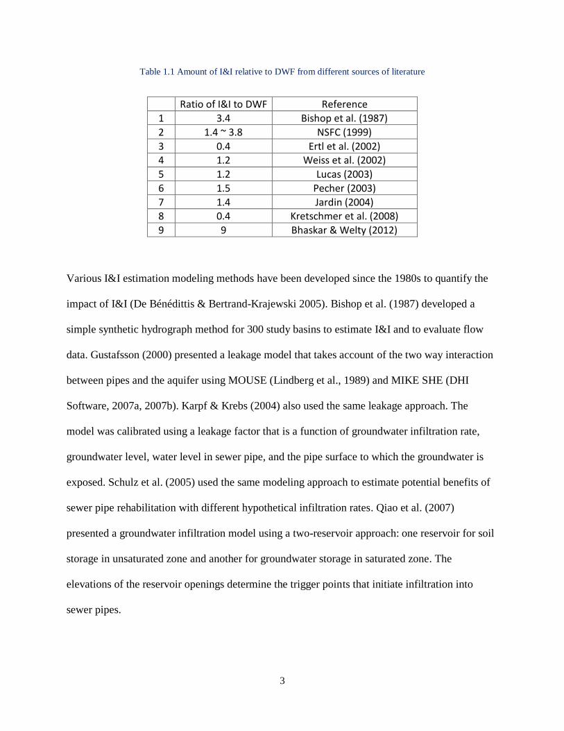
type, etc. Ratios of I&I to dry weather flow (DWF) compiled from a review of literature on this

topic are summarized in Table 1.1. The range of the ratio varies from 0.4 to 10. For example, I&I

for Baltimore City was ten times greater than the DWF, which means 90 percent of the

wastewater flow is I&I. This indicates that I&I volume can affect the capacity of a sanitary sewer

system significantly.

3

Table 1.1 Amount of I&I relative to DWF from different sources of literature

Ratio of I&I to DWF Reference

1 3.4 Bishop et al. (1987)

2 1.4 ~ 3.8 NSFC (1999)

3 0.4 Ertl et al. (2002) 4 1.2 Weiss et al. (2002)

5 1.2 Lucas (2003)

6 1.5 Pecher (2003)

7 1.4 Jardin (2004) 8 0.4 Kretschmer et al. (2008)

9 9 Bhaskar & Welty (2012)

Various I&I estimation modeling methods have been developed since the 1980s to quantify the

impact of I&I (De Bénédittis & Bertrand-Krajewski 2005). Bishop et al. (1987) developed a

simple synthetic hydrograph method for 300 study basins to estimate I&I and to evaluate flow

data. Gustafsson (2000) presented a leakage model that takes account of the two way interaction

between pipes and the aquifer using MOUSE (Lindberg et al., 1989) and MIKE SHE (DHI

Software, 2007a, 2007b). Karpf & Krebs (2004) also used the same leakage approach. The

model was calibrated using a leakage factor that is a function of groundwater infiltration rate,

groundwater level, water level in sewer pipe, and the pipe surface to which the groundwater is

exposed. Schulz et al. (2005) used the same modeling approach to estimate potential benefits of

sewer pipe rehabilitation with different hypothetical infiltration rates. Qiao et al. (2007)

presented a groundwater infiltration model using a two-reservoir approach: one reservoir for soil

storage in unsaturated zone and another for groundwater storage in saturated zone. The

elevations of the reservoir openings determine the trigger points that initiate infiltration into

sewer pipes.

4

One of the most widely used I&I estimation methods is the “RTK method” that was developed

by Camp Dresser & McKee (CDM) Inc. et al. (1985). According to Lai (2008) “the RTK method

is probably the most popular synthetic unit hydrograph (SUH) method” in the stormwater

management field. This method uses three triangular hydrographs to estimate the response times

associated with the effect of fast, moderate, and slow I&I. By linear convolution of the three

hydrographs, the model produces a total response hydrograph calibrated based on comparison to

an observed hydrograph. The RTK model is calibrated using three parameters: R, T, and K for

each hydrograph. Figure 1.1 illustrates the parameters using one of three hydrographs. R is the

fraction of rainfall volume that is accounted for in this hydrograph as entering the sewer system

as rainfall-derived infiltration and inflow (RDII). When three hydrographs are used in the RTK

approach the total fraction of rainfall volume that enters the sewer system as RDII is allocated to

three R components: R1, R2, and R3. R1 is for the fast inflow element while R2 and R3

represent the slower infiltration elements. T is the time to peak in each hydrograph (typically

expressed in hours), and K is the ratio of time of recession to the time to peak. This method is

embedded in EPA SWMM5 (Rossman 2010) and EPA SSOAP toolbox (Vallabhaneni et al.

2008). Despite its popularity, the model does not reflect the underlying physics of each I&I

response so there can be a vast number of possible combinations of the nine RTK parameters.

Also there is a little guidance for calibrating these models and for I&I modeling in general

(Allitt, 2002).

5

Figure 1.1 Three parameters: R, T, and K of the RTK method illustrated with one of three RTK hydrographs

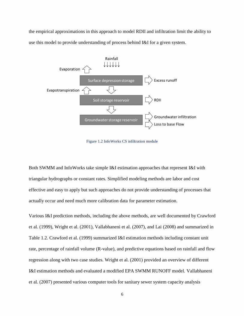
InfoWorks CS (Innovyze 2011) is another popular stormwater modeling tool that has an option

for I&I simulation. InfoWorks simulates I&I using two components: rainfall-induced infiltration,

and groundwater infiltration. This is different from SWMM because the RTK method only takes

into account rainfall induced I&I but not groundwater infiltration. In the InfoWorks CS

infiltration module depicted in Figure 1.2, the percolation flow from the surface depression

storage is assigned to the soil storage reservoir after a runoff occurs. When the soil reaches the

percolation threshold, a proportion of this percolation flow goes to the sewer network. This

represents RDII. The remainder of the percolation flow goes down to the groundwater storage

reservoir. When the groundwater level reaches the sewer system invert level, groundwater

infiltration occurs. The method enables engineers to model groundwater infiltration into a sewer

system but the full physical process is not taken into account. For example, according to the

model assumption, groundwater infiltration occurs when the groundwater level is higher than the

pipe invert elevation not the water level in the sewer pipe. InfoWorks CS is widely used because

it provides easy to use representation of RDII and it is useful for operational design. However,

6

the empirical approximations in this approach to model RDII and infiltration limit the ability to

use this model to provide understanding of process behind I&I for a given system.

Figure 1.2 InfoWorks CS infiltration module

Both SWMM and InfoWorks take simple I&I estimation approaches that represent I&I with

triangular hydrographs or constant rates. Simplified modeling methods are labor and cost

effective and easy to apply but such approaches do not provide understanding of processes that

actually occur and need much more calibration data for parameter estimation.

Various I&I prediction methods, including the above methods, are well documented by Crawford

et al. (1999), Wright et al. (2001), Vallabhaneni et al. (2007), and Lai (2008) and summarized in

Table 1.2. Crawford et al. (1999) summarized I&I estimation methods including constant unit

rate, percentage of rainfall volume (R-value), and predictive equations based on rainfall and flow

regression along with two case studies. Wright et al. (2001) provided an overview of different

I&I estimation methods and evaluated a modified EPA SWMM RUNOFF model. Vallabhaneni

et al. (2007) presented various computer tools for sanitary sewer system capacity analysis

7

including EPA SSOAP tool box. Lai (2008) also presented I&I prediction methods with sewer

design practices. Even though there are many different methods available, none of these methods

were developed based on physical process of I&I. These methods are event specific and the

accuracy of prediction for different rainfall events is not reliable.

8

Table 1.2 Various I&I estimation methods presented in literature

Method Literature Explanation Shortcomings

Constant unit rate Crawford et al. (1999) Lai (2008)

In flowrate per acre

Used for design manuals

Dependent on sewershed area, land use, population, and pipe length for large areas

Difficult to develop reasonable estimate since it may vary temporarily for all storms (Lai 2008)

Percentage of rainfall volume (R-value, R factor, or rational method)

Crawford et al. (1999) Wright et al. (2001) Vallabhaneni et al. (2007) Lai (2008)

R = volume of wet weather RDII/rainfall volumex100

Typically triangular hydrograph shape is used.

Too simple for design or permitting estimates as only volume is considered (Wright et al. 2001)

Percentage of streamflow

Crawford et al. (1999) Lai (2008)

Relationship between sewer flow monitoring data and streamflow data

The sewer system condition and the sewershed area condition need to be consistent

Unit hydrograph Crawford et al. (1999) Wright et al. (2001) Vallabhaneni et al. (2007) Lai (2008)

RDII responds to rainfall volume and duration

Shape of the hydrograph depends on basin characteristics

Several unit hydrographs to represent the separate components contributing to RDII

Linear model based on the assumption that rainfall is constant in time and uniformly distributed in space

UH methods 1) Synthetic unit hydrographs (SUH): RTK method 2) Data-derived UH: the regression method 3) UH derivation using least square regression 4) UH derivation using a linear program 5) Conceptually derived UH

UH is often empirically fit to measurement and has no physical meaning

Probabilistic Crawford et al. (1999) Lai (2008)

Frequency analysis of peak RDII flows (rate or volume)

Relationship of sewer flow to recurrence interval

Rainfall effects are not reflected and the frequency analysis is more adequate for extreme events

9

Besides the I&I estimation modeling in urban hydrology, models of interactions between porous

media flow and buried pipes have been developed and described in the agricultural tile drainage

literature. Some of the agricultural drainage literature related to inflow into buried pipes is

summarized in Table 1.3.

Table 1.3 Summary of the agricultural drainage literature related to modeling

Authors Year Summary of key findings

1 Fipps & Skaggs 1986 Comparison of four different finite element methods for tile drain systems

2 Fipps & Skaggs 1992 Application of numerical solutions to various subsurface drain conditions and development of an approximate method

3 Kim & Delleur 1997 Comparison of physically based storage approach and a new approach using a transfer function, extended TOPMODEL, for tile drain flows

4 Tarboton & Wallender

2000 Comparison of different finite element grid configurations for steady and transient flow to a single drain

5 Cooke & Badiger 2001 Applicability of subsurface drainage theory for single tile system to irregular or random drainage system using unsaturated-flow finite element model

6 Buyuktas & Wallender

2002 Evaluation of a single equivalent soil hydraulic parameter to study water and solute transport to tile drains using three-dimensional deterministic model

7 Carluer & Marsily 2004 Man-made drainage network modeling using distributed watershed model (ANTHROPOG)

8 Purkey et al. 2004 Enhanced deforming finite element model to examine the interactions between tile drainage and a local groundwater table

9 Carlier et al. 2007 Equivalent representation of tile drains using a homogeneous anisotropic porous medium

10

At small scales, applying a detailed physics-based model improves the prediction, yet some

simplification improves practicality. Carlier et al. (2007) presented an equivalent-medium

approach for drains buried in a soil profile, which takes the entire soil column as a uniform layer

with averaged soil properties. Although the water table showed slightly faster response with the

simplified approach, the results provided were still considered reasonable. Despite the

advantages that using a detailed model can provide to understand the infiltration process, this

approach has not been widely used in urban hydrology. Thus, in this study, several I&I processes

are investigated using physics-based models. In particular, the equivalent-medium approach from

Carlier et al. (2007) is adopted to model a leaky sewer lateral, as described in chapter 3.

1.2. Research Objectives

The objective of this study is to understand the hydrologic behavior induced by the I&I process

using physics-based models for three major I&I sources: roof downspout, sump pump

connection, and leaky sewer lateral. In particular, the uncertainty in the rainfall induced

infiltration (RII) and how this impacts hydrological response at sewershed scale are investigated.

In chapter 2, I&I and RII are defined and different I&I sources are summarized. Chapter 2 also

discusses the relative contribution and behavior of different I&I sources and why roof

downspout, sump pump, and leaky lateral are selected as the three representative sources. The

methodology for the I&I modeling and the model calibration using genetic algorithm (GA) is

presented in chapter 3. In chapter 4, physics-based modeling of three I&I sources: roof

downspout, sump pump connection, and leaky sewer lateral, is introduced to better understand

the I&I processes. Unique flow response for each I&I source is derived and the characteristics

11

are compared. The models are applied to Palos Hills, IL and are calibrated using sewer

monitoring data. A GA technique is utilized for the calibration and the widely used RTK method

is also tested for comparison. In addition to the model development, uncertainty associated with

six different model parameters related to the RII process (antecedent moisture condition (AMC),

soil characteristics, pedotransfer functions (PTFs), sewer pipe depth, initial condition, and

rainfall characteristics) is investigated and presented in chapter 5.

12

References

Allitt, R. (2002) Rainfall, runoff and infiltration re-visited. WaPUG Spring Meeting 2002 (pp. 1–

9).

ASCE (2013) Report Card for America’s Infrastructure.

Backmeyer, D. P. (1960) Effects of infiltration. Water Pollution Control Federation 32(5), 539–

540.

Bhaskar, A. S., & Welty, C. (2012) Water balances along an urban-to-rural gradient of

metropolitan Baltimore , 2001 – 2009. Environmental & Engineering Geoscience, XVIII(1),

37–50.

Bishop, W. J., Diemer, D. M. & Wallis, M. J. (1987) Regional infiltration/inflow study solves

wet weather sewer problems. Journal of Water Pollution Control Federation 59(5), 289–

293. Retrieved from http://www.jstor.org/stable/25043247?origin=JSTOR-pdf

Buyuktas, D. & Wallender, W. W. (2002) Numerical simulation of water flow and solute

transport to tile drains. Journal of Irrigation and Drainage Engineering 128(1), 49–56.

Camp Dresser & McKee (CDM) Inc., F.E. Jordan Associates Inc. & James M. Montgomery

Consulting Engineers. (1985) East Bay infiltration/inflow study manual for cost-

effectiveness analysis. Oakland, CA.

13

Carlier, J. P., Kao, C. & Ginzburg, I. (2007) Field-scale modeling of subsurface tile-drained soils

using an equivalent-medium approach. Journal of Hydrology 341(1-2), 105–115.

doi:10.1016/j.jhydrol.2007.05.006

Carluer, N. & Marsily, G. De. (2004) Assessment and modelling of the influence of man-made

networks on the hydrology of a small watershed: implications for fast flow components,

water quality and landscape management. Journal of Hydrology 285(1-4), 76–95.

doi:10.1016/j.jhydrol.2003.08.008

Cooke, R. A. & Badiger, S. (2001) Drainage equations for random and irregular tile drainage

systems. Agricultural Water Management 48, 207–224.

Crawford, D., Eckley, P. & Pier, E. (1999) Methods for estimating inflow and infiltration into

sanitary sewers. New applications in modeling urban water systems, Volume 7, Conference

on Stormwater and Related Water Systems Modeling; Management and Impacts, 299–315.

Toronto: CHI.

De Bénédittis, J. & Bertrand-Krajewski, J. L. (2005) Infiltration in sewer systems: comparison of

measurement methods. Water Science and Technology: a Journal of the International

Association on Water Pollution Research 52(3), 219–27. Retrieved from

http://www.ncbi.nlm.nih.gov/pubmed/16206862

DHI Software. (2007) MIKE SHE user manual volume 1: user guide (Vol. 1).

DHI Software. (2007) MIKE SHE user manual volume 2: reference guide (Vol. 2).

14

Ertl, T. W., Dlauhy, F. & Haberl, R. (2002) Investigations of the amount of infiltration / inflow

into a sewage system. Proceedings of the 3rd “Sewer Processes and Networks”

International Conference. Paris, France.

Field, R., & Struzeski, E. J. (1972) Management and control of combined sewer overflows.

Water Pollution Control Federation, 44(7), 1393–1415.

Fipps, G., & Skaggs, R. W. (1992) Simple methods for predicting flow to drains. Journal of

Irrigation and Drainage Engineering, 117(6), 881–896.

Fipps, G., Skaggs, R. W., & Nieber, J. L. (1986) Drains as a boundary condition in finite

elements. Water Resources Research, 22(11), 1613–1621.

Franz, T. (2007) Spatial classification methods for efficient infiltration measurements and

transfer of measuring results. Dresden University of Technology, Dresden, Germany.

Gottstein, L. E. (1976) Sewer system evaluation for infiltration/inflow. Minneapolis, Minnesota.

Gustafsson, L. (2000) Alternative drainage schemes for reduction of inflow/infiltration -

prediction and follow-up of effects with the aid of an integrated sewer/aquifer model. 1st

International Conference on Urban Drainage via Internet (pp. 21–37).

Innovyze. (2011) InfoWorks CS technical review.

Jardin, N. (2004) Fremdwasser – eine grundsätzliche Problembeschreibung (Extraneous water –

a basic description). Proceedings of 3rd Forum Ruhrverband. Essen, Germany.

15

Karpf, C., & Krebs, P. (2004) Sewers as drainage systems – quantification of groundwater

infiltration. In Novatech 2004, 6th International conference on sustainable techniques and

strategies in urban water managementWater Management (pp. 969–975). Lyon.

Kim, S., & Delleur, J. W. (1997) Sensitivity analysis of extended TOPMODEL for agricultural

watersheds equipped with tile drains. Hydrological Processes, 11, 1243–1261.

Kretschmer, F., Ertl, T., & Koch, F. (2008) Discharge monitoring and determination of

infiltration water in sewer systems. In 11th International Conference on Urban Drainage

(pp. 1–7). Edinburgh, Scotland, UK.

Lai, F. D. (2008) Review of sewer design criteria and RDII prediction methods. Washington,

DC.

Lindberg, S., Nielsen, J. B., & Carr, R. (1989) An integrated PC-modelling system for hydraulic

analysis of drainage systems. Watercomp ’89: The First Australasian Conference on

Technical Computing in the Water Industry. Melbourne, Australia.

Lucas, S. (2003) Auftreten, Ursachen und Auswirkungen hoher Fremdwasserabflüsse – eine

zeitliche und räumliche nalyse (Occurence, causes and effects of high extraneous water

flows). Universität Karlsruhe.

NCPWI (National Council on Public Works Improvement). (1988) Fragile foundations: a report

on America’s Public Works, Final report to the president and congress.

16

NSFC (National Small Flows Clearinghouse). (1999) Infiltration and inflow can be costly for

communities. Pipeline: Small Community Wastewater Issues Explained to the Public,

Vol.10, No.2.

Pecher, K. H. (2003) Fremdwasseranfall, Schwankungen und Konsequenzen für die

Abwasserbehandlung (Amount of I/I, variations and consequences). Proceedings of 36th

Essener Tagung, Gewässerschutz-Wasser-Abwasser. Aachen, Germany.

Petroff, R. G. (1996) An analysis of the root cause of sanitary sewer overflows. In: Seminar

Publication National Conference on Sanitary Sewer Overflows (SSOs): april 24-26, 1995,

Washington D.C., 8–15. Cincinnati, OH: EPA.

Purkey, D. R., Wallender, W. W., Fogg, G. E. & Sivakumar, B. (2004) Describing near surface,

transient flow processes in unconfined aquifers below irrigated lands: Model application in

the Western San Joaquin Valley, California. Journal of Irrigation and Drainage

Engineering 130(6), 451–459. doi:10.1061/(ASCE)0733-9437(2004)130

Qiao, F., Lu, H., Derr, H. K., Wang, M., & Chen, M. (2007) A new method of predicting rainfall

dependent inflow and infiltration. Water Environment Federation (pp. 1883–1890).

doi:10.2175/193864707788116040

Rossman, L. A. (2010) Storm water management model user’s manual version 5.0. Cincinnati,

OH.

Schulz, N., Baur, R., & Krebs, P. (2005) Integrated modelling for the evaluation of infiltration

effects. Water science and technology: a journal of the International Association on Water

17

Pollution Research, 52(5), 215–23. Retrieved from


Sliter, J. T. (1974). Infiltration/inflow guidelines spark controversy. Journal of Water Pollution

Control Federation, 46(1), 6–8.

Tarboton, K. C. & Wallender, W. W. (2000) Finite-element grid configurations for drains.

Journal of Irrigation and Drainage Engineering 126(4), 243–249.

USEPA (2008) Clean Watershed Needs Survey 2008 Report to Congress (EPA-832-R-10-002).

Vallabhaneni, S., Chan, C. C., & Burgess, E. H. (2007) Computer tools for sanitary sewer system

capacity analysis and planning. Cincinnati, OH.

Vallabhaneni, S., Lai, F., Chan, C., Burgess, E. H. & Field, R. (2008) SSOAP − A USEPA

toolbox for sanitary sewer overflow analysis and control planning. EWRI 2008 World

Environmental & Water Resources Congress, May 13-16, 2008. Honolulu, HI: American

Society of Civil Engineers (ASCE).

Weiss, G., Brombach, H. & Haller, B. (2002) Infiltration and inflow in combined sewer systems:

long-term analysis. Water science and technology : a journal of the International



Wright, L., Dent, S., Mosley, C., Kadota, P. & Djebbar, Y. (2001) Comparing rainfall dependent

inflow and infiltration simulation method. In: Models and Applications to Urban Water

Systems. Monograph 9, 235–258. Toronto, Ontario, Canada: CHI.

18

2. Literature Review

In this chapter, definitions of I&I that have appeared in the literature are presented. Various I&I

sources are discussed and three common methods to estimate the I&I flow in a sewer system are

introduced. In addition, spatial and temporal variability of I&I sources in a sewershed are

investigated.

2.1. Definition and Sources of I&I

Infiltration and inflow (I&I) are extraneous water that enters into both sanitary and combined

sewer systems unintentionally. Since sanitary sewer systems are designed only for wastewater

I&I is also called ‘parasite water.’ The urban hydrologic literature contains a variety of

definitions of I&I. One from the EPA is as follows (EPA 1995):

“Inflow means that water enters the sewer system from the land’s surface in an

uncontrolled way. Usually, this happens when surface water runs in through unsealed

manhole covers. It may also happen when people illegally connect their foundation

drains, roof leaders, cellar drains, yard drains, or catch basins to the sewer system.”

“Infiltration happens when non-wastewater seeps into the sewer system from the ground.

Ground water usually leaks into the sewer system through defective pipes, pipe joints,

connections, or manholes.”

Since inflow is originated from direct connections, the flow response is nearly immediate and

flow peaks are large. Contrarily, infiltration shows slow and persistent responses in time. Belhadj

et al. (1995) described the differences between infiltration and inflow in terms of behaviors.

Inflow displays high peak flows that are directly related to rainfall events. In contrast, infiltration

19

creates slow change in flow. These flow characteristics have been also well recognized in the

field of sewer management and rehabilitation (Peters & Troemper 1969).

According to the definition of I&I, there are various I&I sources (Table 2.1). Any direct

connection in a sanitary sewer system to the surface water is an inflow source. These include

roof downspout, floor drain, unsealed manhole cover, storm sewer connections, etc. Compared to

inflow sources, infiltration sources are simple; any groundwater intrusion through pipe and

manhole defects. Root intrusion was recognized as a major sewer system problem (Sullivan et al.

1977b) that exacerbates infiltration problem. Images of roots growing through pipe joints and

cracks are presented in Table 2.1. Gaps in the joints and cracks between pipes and manholes

allow ground water to enter the sewer pipes. Depending on the pipe material and age, these

faulty sewers can cause a great amount of sewer infiltration.

Barnard et al. (2007) classified I&I into fast, medium, and slow responses. Medium response is

defined as “more delayed and attenuated response to rainfall” and this is also referred to as

“rapid infiltration.” Hodgson & Schultz (1995) used footer drain as an example of the medium

response. Nogaj & Hollenback (1981) pointed out that foundation drains and storm sumps are

not expected to be highly sensitive to changes in rainfall intensity, which makes these inflow

sources classified as medium sources. The RTK method also takes three triangular hydrographs

to estimate I&I flow: one for a short-term response, one for an intermediate-term response, and

one for a long-term response (Rossman 2004). Thus the inflow sources in Table 2.1 are further

divided into the medium and fast responses.

20

Table 2.1 Possible I&I sources

Infiltration Inflow Slow Medium Fast

Defective pipes and manhole walls, Pipe joints, Connections

Sump pumps, Foundation drains, Drains from springs and swampy areas

Roof leaders, Cellar, Yard drains, Patio drains, Area drains, Driveway, Sidewalk, Stairwell drains, Window well drains, Cooling water discharges, Cross connections from storm sewers and combined sewers, Catch basins, Storm sewers, Surface run-off, Street wash water, Drainage, Floor drains, Removed sewer cleanout caps, Leakage from drinking water networks, Manhole covers

Figure 2.1 Root intrusion through cracks and joints of sewer pipes (Images from Urbana Champaign Sanitary

District 2012)

21

2.2. Methods to Estimate I&I

The amount of I&I ( &I IQ ) in the measured sewer flow ( sewerQ ) can be estimated by subtracting

the amount of DWF ( DWFQ );

&I I sewer DWFQ Q Q

The I&I portion of the flow in a sewer system can be estimated using these methods (De

Bénédittis & Bertrand-Krajewski, 2005a, Ertl, 2002, Franz 2007):

1) Statistical method (flow-based method, hydraulic method, quantitative method)

2) Chemical method (pollutant-based method, qualitative method)

3) Drinking water consumption comparison

The statistical method, also called a flow-based, hydraulic, or quantitative method, uses sewer

flow measurements during specified conditions or periods (e.g. residual night flow) to obtain

domestic wastewater flows. This method is easily applicable since it only requires flow

measurements while the other two methods demand extra measurement or analysis on top of

flow measurement (Kretschmer et al. 2008). The chemical method, also called a pollutant-based,

or qualitative method, uses pollutant concentrations e.g. COD, BOD, ammonia, iron in the

sewage discharge and average pollutant discharge per capita (Verbanck et al. 1989, Kracht &

Gujer 2005, Bareš 2009). Some physical properties e.g. turbidity, conductivity, and temperature

have been also used as I&I indicators with simple dilution relationship (Veldkamp et al. 2002,

Aumond & Joannis 2005, Schilperoort 2006, Aumond & Joannis 2008). Instead of using natural

pollutants or physical property of DWF, artificial tracer can be used to estimate sewer infiltration

22

(Verbanck 1993). De Bénédittis & Bertrand- Krajewski (2005b) introduced an infiltration

estimation method using oxygen isotopes, 18O, as conservative natural tracers in Lyon, France.

The new method was developed based on the difference in oxygen isotope concentration in the

ambient groundwater and the drinking water source in the study area. Kracht et al. (2007) also

used natural isotopes of water (18O/16O and D/H) to quantify sewer infiltration. Pitterle &

Mcginnis-Carter (2010) introduced optical brighteners to identify sewer point sources. Optical

brighteners are frequently found in laundry detergent and most household wastewater contains

laundry detergent. This substance has been used to track fecal contamination in ambient water

but has not been widely applied to I&I estimation except a recent ongoing study by P. Miller & J.

Dunker (personal communication, September 26, 2013). The drinking water consumption

method uses the number of inhabitants in the study area multiplied by the average value of

sewage discharge per capita. Whichever method is selected, sewer monitoring is necessary to

obtain I&I hydrograph.

De Bénédittis & Bertrand-Krajewski (2005a) examined 13 different I&I estimation methods,

including 11 variants of the statistical (flow-based) method and two variants of the chemical

method. Their results showed great variability in the estimated flow volume among the methods.

They found that infiltration amounts from the methods vary by as much as 20% of total DWF.

To avoid a large uncertainty, at least 8 to 10 days of DWF observation was recommended for the

methods that use minimum night flow.

As older sewer systems started aging and experiencing I&I problems in the 1960’s and 1970’s,

many field surveys and inspections were performed and sewer rehabilitation techniques were

developed. It was not until 1970s when the most urban communities in the US started to restrict

the stormwater flow into sanitary sewers (Gottstein 1976, Barnard et al. 2007). Based on sewer

23

Table 2.2 Sewer inspection and rehabilitation techniques in 1960’s and 1970’s

Authors Year Summary of key findings

1 Borland 1956 Experimental study about the relation between sewer infiltration and exfiltration

2 Stacy 1961 Smoke testing to locate leaky sewers

3 Dahlmeyer 1962 Chemical seal technique to stabilize soil and stop sewer infiltration

4 Van Natta 1963 Stiffer requirements in the plumbing ordinances to reduce sewer infiltration

5 Santry 1964 Experimental study about leaky sewer pipe depending on varying depths of submergence and improved pipe joints to minimize infiltration

6 Stepp 1967 Chemical sealing technique to resolve sewer infiltration problem

7 Haugh 1969 Techniques and challenges to coat leaky concrete sewer under damp conditions

8 Public Works 1969 Pictures of root intrusion, broken pipe, and leaky sewer from sewer inspection

9 American Public Works Association

1970 Thorough national study project to understand I&I problems and its impact on sewer systems

10 American Public Works Association

1971 A Manual of Practice composed from American Public Works Association (1970) about prevention and correction of I&I

11 Montgomery County Sanitary Department

1972 The effect of infiltration reduction by joint sealing and closed circuit television techniques

12 Welker and Miller 1974 Detection of illegal connections using smoke test

13 Gutierrez & Wilmut

1975 I&I requirements of the EPA and the feasibility of elimination effort

14 Lutz 1976 Split of I&I hydrograph into infiltration and inflow components

15 Kranik & Johnson 1976 Sewer system evaluation and survey to reduce I&I 16 Maynes 1976 Sewage flow data collection and cost estimate from I&I

17 Elliott et al. 1977 The effectiveness of I&I from private properties

18 Stilley 1977 Required field operations for an I&I analysis

19 Sullivan et al. 1977a A Manual of Practice for sewer system evaluation, rehabilitation and new construction

20 Public Works 1979 Effectiveness of watertight manhole inserts to remove stormwater inflow through manhole covers

24

evaluation and cost analysis studies, many cities realized that repairing damaged sewer systems

is more economical than expanding the treatment facility (Podolick 1975). The efforts to

calculate I&I based on measurements are summarized in Table 2.2Error! Reference source not

found.. Note that these are all measurement methods, rather than predictive estimation methods

presented in chapter 1.

2.3. Space and Time Variability of I&I Process

Each community experiences I&I differently and the major I&I source varies in a particular

sewershed. In fact, many different factors affect I&I characteristics: climate, geography, soil

characteristics, groundwater table condition, construction material, pipe joint types, pipe age,

vegetation, workmanship, construction procedure, and existence of illegal connections. Belhadj

et al. (1995) also stressed that RDII is highly temporally and spatially variable depending on the

rainfall intensity, groundwater level, and soil moisture.

Seasonal variability is one of the common temporal variabilities in sewer flow. Ertl et al. (2002)

discovered a seasonal variation in I&I by analyzing the inflow to a water treatment plant in east

Austria. Increased I&I were observed in spring and autumn depending on the groundwater level

in the study area. Kretschmer et al. (2008) also analyzed DWF monitoring data with monthly

variation in Austria; high in spring and low in summer. Brombach et al. (2002) showed the

seasonal variability can be up to 10 times in the high infiltration season compared to the low

season. Flooding also raises the local groundwater level and increases I&I (Karpf & Krebs,

2004). This can affect I&I greatly in places with high seasonality in rainfall.

25

Temporal variability also exists at smaller scales. De Bénédittis & Bertrand-Krajewski (2005b)

found strong variations in the hydrograph of infiltration during a day. Two flow peaks were

observed in the I&I hydrograph due to the connections of groundwater pumps, and the low DWF

depth during nights. Low DWF level in sewer pipes exposes more pipe defects hence increases

the infiltration flow during night time as the hydraulic gradient between the wastewater surface

level and the groundwater level around the sewer increases.

Antecedent moisture condition (AMC) is an important factor that affects temporal variability of

I&I (Czachorski & Van Pelt 2001, Van Pelt & Czachorski 2011, Sadri & Graham 2011). AMC is

one source of non-linearity of I&I and Czachorski & Van Pelt (2001) applied a nonlinear system

identification method, which is commonly used in aerospace engineering applications for high

fidelity modeling of aircraft and space system, to model I&I. Sadri & Graham (2011) suggested a

regression method to predict I&I including the AMC for past 10 days. Not many commercial

models take account of AMC in I&I estimation. The i3D antecedent moisture (i3D AM) model

considers AMC using the system identification technique from aerospace engineering control

systems (i3D Technologies, 2010). Investigation about AMC related to infiltration process is

covered in the chapter 5 in this thesis.

Inherently I&I has spatial variability, since it is affected by spatially varied parameters such as

the age of sewer system, local groundwater condition, etc. Franz (2007) developed a method to

optimize infiltration flow measurement locations in a sewer system. To improve the information

yield, measurement results from identified measuring locations are paired with other potential

measuring points by comparing sub-catchments and classifying reaches. This method is based on

the ‘similarity approach’ and multivariate statistical techniques. The similarity approach is based

26

on the assumption that similar sewer conditions yield similar I&I rates. This optimization method

improved the accuracy of I&I estimations by 40%.

References

American Public Works Association. (1970) Control of infiltration and inflow into sewer systems

(p. 133).

American Public Works Association. (1971) Prevention and correction of excessive infiltration

and inflow into sewer systems: A manual of practice (p. 125).

Aumond, M., & Joannis, C. (2005) Turbidity monitoring in sewage. 10th International

Conference on Urban Drainage. Copenhagen, Denmark.

Aumond, M., & Joannis, C. (2008) Processing sewage turbidity and conductivity recorded in

sewage for assessing sanitary water and infiltration/inflow discharges. 11th International

Conference on Urban Drainage (pp. 1–10). Edinburgh, Scotland, UK.

Barnard, T. E., Whitman, B. E., Hill, C., Mckay, G., Plante, S., & Schmitz, B. A. (2007)

Wastewater collection system modeling and design-CH7 (1st ed., pp. 203–270). Bentley

Institute Press.

Bareš, V., Stránský, D., & Sýkora, P. (2009) Sewer infiltration/inflow: long-term monitoring

based on diurnal variation of pollutant mass flux. Water Science and Technology : a Journal

of the International Association on Water Pollution Research, 60(1), 1–7.

doi:10.2166/wst.2009.280

27

Belhadj, N., Joannis, C., & Raimbault, G. (1995) Modelling of rainfall induced infiltration into

separate sewerage. Water Science & Technology, 32(1), 161–168.




Borland, S. (1956) “New data on sewer infiltration-exfiltration ratios.” Public Works Sep. 1956:

97–98.

Blöschl, G. & Sivapalan, M. (1995) Scale issues in hydrological modelling: A review.

Hydrological Processes 9, 251–290.

Brombach, H., Weiss, G., & Lucas, S. (2002) Temporal variation of infiltration inflow in

combined sewer systems. Proceedings of 9th International Conference on Urban Drainage

(9ICUD), 112, 125–125. doi:10.1061/40644(2002)125

Czachorski, R. S. & Pelt, T. H. Van. (2001) On the modeling of inflow and infiltration within

sanitary collection systems for addressing nonlinearities arising from antecedent moisture

conditions. WEFTEC, 606.

Dahlmeyer, F. D. (1962) “Chemical seal stops sewer infiltration.” Public Works Nov. 1962: 91–

92.

De Bénédittis, J. & Bertrand-Krajewski, J. L. (2005a) Infiltration in sewer systems: comparison

of measurement methods. Water Science and Technology : a Journal of the International

28



De Bénédittis, J., & Bertrand-Krajewski, J. L. (2005b) Measurement of infiltration rates in urban

sewer systems by use of oxygen isotopes. Water science and technology: a journal of the

International Association on Water Pollution Research, 52(3), 229–37. Retrieved from


Elliott, J. C., Hydro, S. K., MAlarich, M. A., & Weaver, W. (1977) “Removing private sources

of infiltration and inflow.” Water Environment & Technology Aug. 1977: 55–60.

EPA. (1985) Infiltration/inflow: I&I analysis and project certification. Environmental Protection,

8. Washington, DC.

EPA. (1991) Sewer system infrastructure analysis and rehabilitation (p. 92). Cincinnati, OH.

EPA. (1995) Federal Register 60(234), 62546–62659.

Ertl, T. W., Dlauhy, F., & Haberl, R. (2002) Investigations of the amount of infiltration/inflow

into a sewage system. In Proceedings of the 3rd “Sewer Processes and Networks”





29

Gutierrez, A. F., & Wilmut, C. (1975) “The feasibility of infiltration/inflow elimination.” Public

Works Apr. 1975: 68–70.

Haugh, H. H. (1969) “Rehabilitation of a concrete sewer under infiltration pressure.” Public

Works Jul. 1969: 89–90.

Hodgson, J.E., Schultz, N.U., (1995) Sanitary sewage discharges in the city of Edmonton,

Alberta, pp. 403-413, in Seminar Publication: National Conference on Sanitary Sewer

Overflows (SSOs) (p. 588). Washington D.C.

i3D Technologies. (2010) Technical overview: The i3D antecedent moisture model.




Kracht, O., Gresch, M., & Gujer, W. (2007) A stable isotope approach for the quantification of

sewer infiltration. Environmental Science and Technology technology, 41(16), 5839–45.

Retrieved from http://www.ncbi.nlm.nih.gov/pubmed/17874795

Kracht, O., & Gujer, W. (2005) Quantification of infiltration into sewers based on time series of

pollutant loads. Water Science and Technology : a Journal of the International Association

on Water Pollution Research, 52(3), 209–18. Retrieved from


30




Lutz, J. J. (1976) “Comparing inflow and infiltration.” Water & Sewage Works May 1976: 68–

69.

Maynes, J. S. (1976) Flow data collection for infiltration-inflow analysis. Journal of Water

Pollution Control Federation, 48(8), 2055– 2061. Retrieved from

http://www.jstor.org/stable/25039977 .

Montgomery County Sanitary Department. (1972) Ground water infiltration and internal sealing

of sanitary sewers (p. 75). Montgomery County, Ohio.

Nogaj, R. J., & Hollenbeck, A. J. (1981) One technique for estimating inflow with surcharge

conditions. Journal of Water Pollution Control Federation, 53(4), 491–496.

Peters, G. L. & Troemper, A. P. (1969) Reduction of hydraulic sewer loading by downspout

removal. Water Pollution Control Federation 41(1), 63–81.

Pitterle, B., & Mcginnis-Carter, F. (2010) Optical brightener monitoring in Goleta streams: A

summary of monitoring results from August 2009 - November 2009, (January).

Podolick, P. A. (1975) Preparing an infiltration/inflow analysis. Water & Sewage Works

Reference Number, 1 TAB, 31–32, 34.

Public Works. (1969) “From the inspector’s photo album.” Public Works Jan. 1969: 73.

31

Public Works. (1979) “Manhole inserts abate inflow.” Public Works Dec. 1979: 47.

Rossman, L. A. (2004) Storm water management model user’s manual: Version 5.0. Cincinnati,

OH.

Sadri, S. & Graham, E. (2011) Development of an antecedent moisture condition model for

prediction of Rainfall-Derived Inflow/Infiltration (RDII). American Geophysical Union.

San Francisco.

Santry, I. W. J. (1964) Infiltration in sanitary sewers. Journal of Water Pollution Control

Federation, 36(10), 1256– 1262. Retrieved from http://www.jstor.org/stable/25035156

Schilperoort, R. P. S., Gruber, G., Flamink, C. M. L., Clemens, F., & Van der Graaf, J. H. J. M.

(2006) Temperature and conductivity as control parameters for pollution-based real-time

control. Water Science & Technology, 54(11), 257. doi:10.2166/wst.2006.744

Stacy, C. E. (1961) “Locating leaky sewers with smoke.” Public Works Nov. 1961: 133.

Stepp, S. G. (1967) “Sealing process resolves infiltration problem.” Public Works Jul. 1967: 70–

73.

Stilley, S. H. (1977) Simulated field study for I&I analysis. Public Works, 50–53.

Sullivan, R. H., Cohn, M. M., Clark, T. J., Thompson, W., & Zaffle, J. (1977a) Sewer system

evaluation, rehabilitation and new construction: A manual of practice (p. 194). Chicago,

IL.

32

Sullivan, R. H., Gemmell, R. S., Schafer, L. A., & Hurst, W. D. (1977b) Economic analysis, root

control, and backwater flow control as related to infiltration/inflow control (p. 114).

Edison, NJ.

Van Pelt, T. H. & Czachorski, R. S. (2011) The application of system identification to inflow and

infiltration modeling and design storm event simulation for sanitary collection systems.

WEFTEC 2011. Los Angeles, CA.

Van Natta, W. S. (1963) “Fighting infiltration into sewers.” Public Works Jul. 1963: 158–159.

Veldkamp, R., Henckens, G., Langeveld, J., & Clemens, F. (2002) Field data on time and space

scales of transport processes in sewer systems. In E. W. Strecker & W. C. Huver (Eds.),

Urban Drainage 2002 (Vol. 112, pp. 293–293). Portland, Oregon: Asce.

doi:10.1061/40644(2002)293

Verbanck, M. A. (1993) A new method for the identification of infiltration waters in sanitary

flows. Water Science & Technology, 27(12), 227–230.

Verbanck, M., Vanderborght, J.-P., & Wollast, R. (1989) Major ion content of urban wastewater:

Assessment of per capita loading. Water Pollution Control Federation, 61(11/12), 1722–

1728.

Welker, F. S., & Miller, D. J. (1974) “Smoke tests detect sources of illegal inflow.” Public

Works Sep. 1974: 90–91.

33

3. Methodology

In this chapter, it is hypothesized that a space and time tradeoff in a local response and a system

response of I&I exists. Roof drain connection, sump pump connection, and leaky sewer lateral

are selected as three main I&I sources and physics-based models to derive impulse response

functions (IRFs) of the three sources are presented. Based on the assumption that spatial

distribution of various I&I sources is negligible in a small sewershed, three main I&I responses

are convoluted. The assumption is based on the discussion about space and time scale tradeoff

that is presented in section 3.2. The genetic algorithm (GA) that is used to calibrate a system

response of I&I is also introduced.

3.1. Introduction

Various efforts have been made to estimate I&I but they are largely empirical. The RTK method,

which is one of the most commonly used I&I estimation methods, uses three triangular

hydrographs to represent various I&I sources. By adjusting nine parameters to fit to sewer flow

monitoring data total I&I is estimated for a sewer system. The parameters determine the peak,

time to peak, and duration of the three triangular hydrographs-three parameters for each

hydrograph. The RTK method has been widely used because of its simplicity and decent

estimation of I&I; however, the RTK method lacks physical meaning of I&I processes.

In this study, a conceptualized model, which better reflects physics of the I&I processes, is

introduced. The basic framework of the model falls under the category of the unit hydrograph

method, as does the RTK method, but three I&I impulse response functions (IRFs) are derived

using physics-based models. Among numerous I&I sources, three most typical sources are

selected to represent three IRFs: inflow from roof connections, sump pump connections, and

34

infiltration through leaky sewer laterals. I&I is originated from mostly private properties (Strand

Associate Inc. 2006), not from main sewer system, which makes it difficult to control. For

simplicity, a single private residential lot is selected as the model domain.

Roof connections are used in this research to represent all the direct connections into a sanitary

sewer system from impervious surfaces (e.g. roof, paved driveways, outdoor stairwells, window

wells). Golden (1995) and Peters & Troemper (1969) showed roof connections are one of the

most problematic I&I sources. Sump pump connections represent “promoted” percolation flow,

which is all the I&I sources that involve mixture of short porous flow and flow through direct

connections at the same time. The word “promoted” is used to describe infiltration that is

facilitated by introducing engineered soil. Reynolds (1995) indicated that roof drains and sump

pumps were suspected to be two major contributors of I&I in the city of South Portland. Longer

flow through porous media, or percolation flow, is represented by the infiltration through leaky

sewer laterals. Pawlowski et al. (2013) indicated that 98% of I&I volume was originated from

downspouts (roof connections) and leaky laterals in the city of Columbus, OH.

The roof connection IRF is developed using the kinematic wave equation (for roof runoff) and

level-pool routing, weir, and orifice flow equations (for rain gutter flow). The influence of the

flow in the roof downspout and the extended connection to the sewer pipe on the time of

concentration is ignored since it is mainly fast vertical flow.

The sump pump connection and the leaky lateral IRFs are developed using the gravity equation

imbedded in the MIKE-SHE (DHI Software 2007a, DHI Software 2007b) which is a spatially

distributed detailed model. Three different soil properties are selected to represent ambient soil,

impervious surface, and highly pervious soil. The equivalent medium approach (Carlier et al.

35

2007) that uses a single soil layer to imitate a leaky lateral and surrounding backfill is applied to

the leaky lateral model.

The IRF from the roof connection shows a high peak and relatively short duration as it represents

runoff from an impervious surface. The leaky lateral IRF shows a low peak and long duration

since the process involves flow through porous media. The IRF from the sump pump connection

falls in between that of the roof connection and the leaky lateral. These three IRFs reflect the

physical characteristics of each I&I process instead of expressing I&I using arbitrary triangular

unit responses as in the RTK method. Roof connection IRF is dominated by the rainfall

hyetograph. The travel time of the flow is short and transformation is negligible. Sump pump

flow path through porous media is short and the media is usually disturbed and modified near

building foundation. Thus the uncertainty associated with the roof connection IRF and the sump

pump IRF is probably small compared to the IRF of infiltration through leaky sewer pipes. RII is

distributed throughout the sewer system and affected by wide variety of pipe depths, media

properties, compaction of soil, etc. Hence, variability in the IRF of RII is anticipated to be much

greater and more significant than for roof connection and sump pump. Therefore, the variability

in RII is further examined in this study while the variability in roof connection and sump pump is

left for future research.

Following six factors are investigated to examine the variability of RII: antecedent moisture

condition (AMC), pedotransfer functions (PTFs), soil hydraulic conductivities, initial conditions

(IC), sewer pipe depths, and rainfall characteristics. To understand the effect of AMC on RII

hydrograph, a uniform rainfall is added to an actual historical rainfall record at ten random time

which results in different AMC conditions for each case. The differences in modeled sewer flow

responses between the actual rainfall and the rainfall with the added storm are used to estimate

36

the infiltration IRF. The effect of soil hydraulic conductivity on RII hydrograph is tested using

14 different conductivity values that are selected from the actual soil data. Seven different PTFs

are applied for the same soil data to compare soil hydraulic conductivity values. Ten different

simulation periods are tested to investigate the effect of IC on the RII hydrograph. The effect of

rainfall characteristics on the RII hydrograph is investigated using various storm durations and

shapes. Eleven different sewer pipe depths are tested to see the effect on RII hydrograph. This

study is mainly focused on examining how the output – RII hydrograph – changes depending on

the change of these six input parameters within anticipated ranges. Any correlation between the

six factors is neglected and each factor is investigated one at a time. Details about the

investigation are discussed in chapter 5.

3.2. Space and Time Scale of I&I Processes

Figure 3.1 shows the spatial and temporal scales of different urban hydrology components. There

is an overall tendency that as the temporal scale increases the spatial scale also increases for a

certain hydrological process. This can be interpreted that once the temporal scale becomes large

smaller spatial variations become less important. In a sewershed, the response time of a local I&I

process relative to the time scale of sewer flow in the entire system determines how important it

is to consider the spatial variability of the I&I processes. If the time scale of a local I&I process

is much smaller than that of the sewer flow in the system, where the I&I enters the system

becomes important. If the time scale of a local I&I process becomes as large as that of the

system, then spatial distribution of the local sources becomes not as important. Thus there is a

tradeoff between time and space.

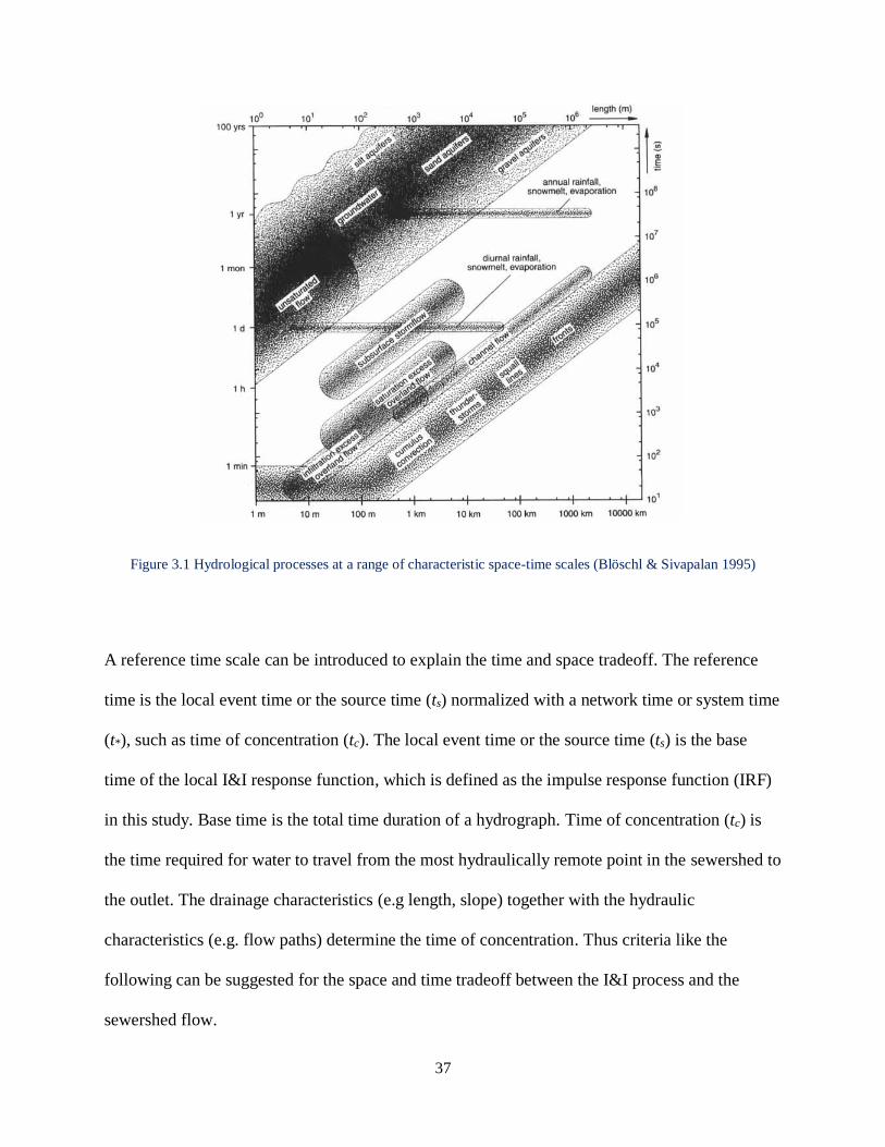
37

Figure 3.1 Hydrological processes at a range of characteristic space-time scales (Blöschl & Sivapalan 1995)

A reference time scale can be introduced to explain the time and space tradeoff. The reference

time is the local event time or the source time (ts) normalized with a network time or system time

(t*), such as time of concentration (tc). The local event time or the source time (ts) is the base

time of the local I&I response function, which is defined as the impulse response function (IRF)

in this study. Base time is the total time duration of a hydrograph. Time of concentration (tc) is

the time required for water to travel from the most hydraulically remote point in the sewershed to

the outlet. The drainage characteristics (e.g length, slope) together with the hydraulic

characteristics (e.g. flow paths) determine the time of concentration. Thus criteria like the

following can be suggested for the space and time tradeoff between the I&I process and the

sewershed flow.

38

When 𝑡𝑠

𝑡∗≪ 1, spatial distribution of I&I sources becomes more important

When 𝑡𝑠

𝑡∗≫ 1, spatial distribution of I&I sources becomes less important

The ratio between the local time scale and the network time scale can be an important factor for

I&I routing in a sewer network. When the ratio is small, spatial distribution of I&I sources in the

network may become important. If the ratio is large, it might not be as important. This shows the

tradeoff between the temporal scales and spatial distribution of I&I responses.

To understand the spatial variability of I&I sources, characteristics of system responses are

investigated in Figure 3.2 and Figure 3.3. Note that the I&I responses that are covered in the later

chapters in this thesis are IRF at a lot scale rather than a system scale. The spatial distribution of

I&I sources in a system is uncertain because it depends on unknown factors such as pipe age,

pipe condition, root intrusion, crack size and location, etc. (Figure 3.2). This means the

distribution of the I&I sources in the system can be viewed as random. Thus it is impractical and

nearly impossible to distinguish every source in the system. Not only I&I but also DWF enters in

many different locations, but the locations of DWF are more predictable as the sewer inlets are

built around the DWF sources.

39

Figure 3.2 Random I&I and DWF input locations in a sewer system

Figure 3.3 shows how the travel time of flow in a sewer network affects fast and slow I&I

sources when the entire system response is taken into consideration. The IRF for a lot scale I&I

source can be identified and from this the I&I responses for a specified rainfall event can be

derived for fast and slow I&I. Both fast and slow I&I enter into the sewer system in three

different locations that are marked with an X, triangle, and circle in the figure; from a shorter to a

longer path. At the downstream outlet of the sewer network (marked with an upside-down

triangle), the system responses for the fast and the slow I&I can be estimated as is shown. The

local responses of the three fast I&I are easier to distinguish from each other in the system

response while that of the three slow I&I are harder as they overlap to a greater extent. The

difference in travel time from the I&I inflow locations to the sewershed outlet among different

sources is negligible for slow I&I because the characteristic time (base time) of the IRF is long

relative to the travel time. In contrast for fast I&I, when the base time is short relative to the

travel time, the locations of the I&I inflow become important. The spatial variability of fast I&I

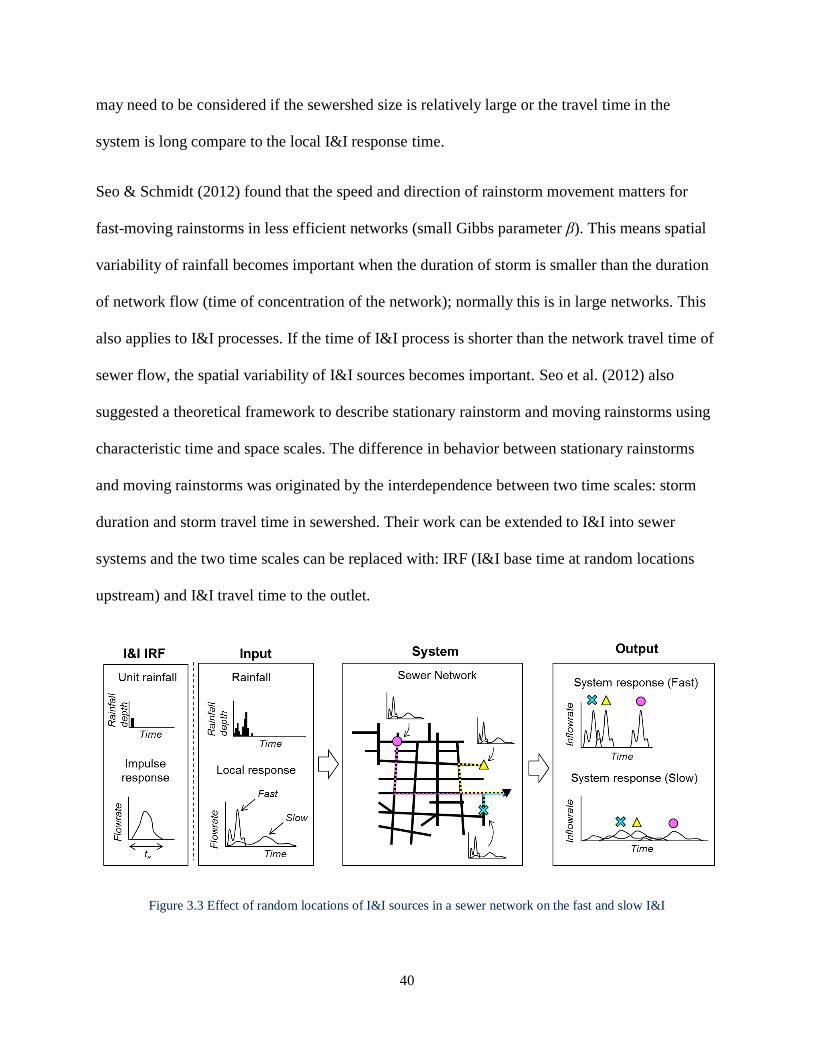
40

may need to be considered if the sewershed size is relatively large or the travel time in the

system is long compare to the local I&I response time.

Seo & Schmidt (2012) found that the speed and direction of rainstorm movement matters for

fast-moving rainstorms in less efficient networks (small Gibbs parameter β). This means spatial

variability of rainfall becomes important when the duration of storm is smaller than the duration

of network flow (time of concentration of the network); normally this is in large networks. This

also applies to I&I processes. If the time of I&I process is shorter than the network travel time of

sewer flow, the spatial variability of I&I sources becomes important. Seo et al. (2012) also

suggested a theoretical framework to describe stationary rainstorm and moving rainstorms using

characteristic time and space scales. The difference in behavior between stationary rainstorms

and moving rainstorms was originated by the interdependence between two time scales: storm

duration and storm travel time in sewershed. Their work can be extended to I&I into sewer

systems and the two time scales can be replaced with: IRF (I&I base time at random locations

upstream) and I&I travel time to the outlet.

Figure 3.3 Effect of random locations of I&I sources in a sewer network on the fast and slow I&I

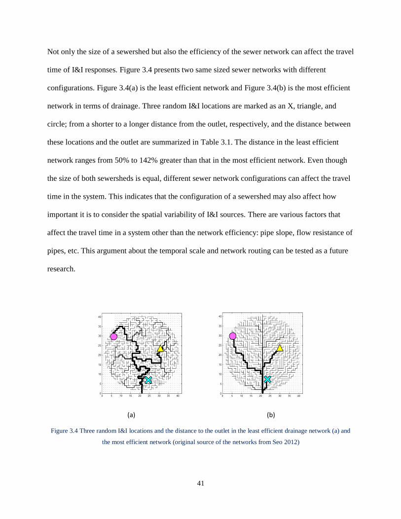
41

Not only the size of a sewershed but also the efficiency of the sewer network can affect the travel

time of I&I responses. Figure 3.4 presents two same sized sewer networks with different

configurations. Figure 3.4(a) is the least efficient network and Figure 3.4(b) is the most efficient

network in terms of drainage. Three random I&I locations are marked as an X, triangle, and

circle; from a shorter to a longer distance from the outlet, respectively, and the distance between

these locations and the outlet are summarized in Table 3.1. The distance in the least efficient

network ranges from 50% to 142% greater than that in the most efficient network. Even though

the size of both sewersheds is equal, different sewer network configurations can affect the travel

time in the system. This indicates that the configuration of a sewershed may also affect how

important it is to consider the spatial variability of I&I sources. There are various factors that

affect the travel time in a system other than the network efficiency: pipe slope, flow resistance of

pipes, etc. This argument about the temporal scale and network routing can be tested as a future

research.

(a) (b)

Figure 3.4 Three random I&I locations and the distance to the outlet in the least efficient drainage network (a) and

the most efficient network (original source of the networks from Seo 2012)

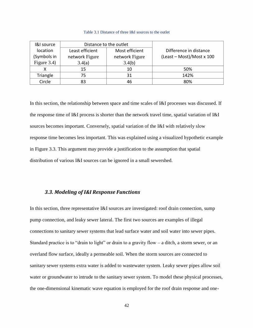
42

Table 3.1 Distance of three I&I sources to the outlet

I&I source location

(Symbols in Figure 3.4)

Distance to the outlet Difference in distance

(Least – Most)/Most x 100 Least efficient

network Figure

3.4(a)

Most efficient network Figure

3.4(b)

X 15 10 50% Triangle 75 31 142%

Circle 83 46 80%

In this section, the relationship between space and time scales of I&I processes was discussed. If

the response time of I&I process is shorter than the network travel time, spatial variation of I&I

sources becomes important. Conversely, spatial variation of the I&I with relatively slow

response time becomes less important. This was explained using a visualized hypothetic example

in Figure 3.3. This argument may provide a justification to the assumption that spatial

distribution of various I&I sources can be ignored in a small sewershed.

3.3. Modeling of I&I Response Functions

In this section, three representative I&I sources are investigated: roof drain connection, sump

pump connection, and leaky sewer lateral. The first two sources are examples of illegal

connections to sanitary sewer systems that lead surface water and soil water into sewer pipes.

Standard practice is to “drain to light” or drain to a gravity flow – a ditch, a storm sewer, or an

overland flow surface, ideally a permeable soil. When the storm sources are connected to

sanitary sewer systems extra water is added to wastewater system. Leaky sewer pipes allow soil

water or groundwater to intrude to the sanitary sewer system. To model these physical processes,

the one-dimensional kinematic wave equation is employed for the roof drain response and one-

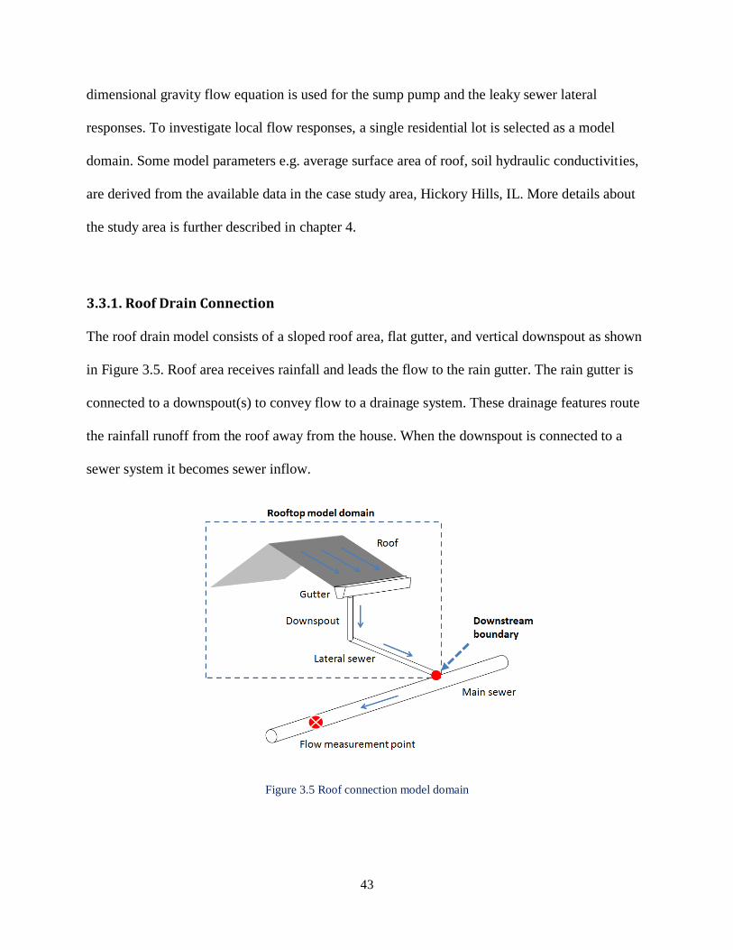
43

dimensional gravity flow equation is used for the sump pump and the leaky sewer lateral

responses. To investigate local flow responses, a single residential lot is selected as a model

domain. Some model parameters e.g. average surface area of roof, soil hydraulic conductivities,

are derived from the available data in the case study area, Hickory Hills, IL. More details about

the study area is further described in chapter 4.

3.3.1. Roof Drain Connection

The roof drain model consists of a sloped roof area, flat gutter, and vertical downspout as shown

in Figure 3.5. Roof area receives rainfall and leads the flow to the rain gutter. The rain gutter is

connected to a downspout(s) to convey flow to a drainage system. These drainage features route

the rainfall runoff from the roof away from the house. When the downspout is connected to a

sewer system it becomes sewer inflow.

Figure 3.5 Roof connection model domain

44

The flow from the roof is calculated using the one-dimensional kinematic wave model for

rainfall-runoff. Two governing equations describe the rainfall-runoff process when using

kinematic wave theory: one-dimensional continuity equation for unit width of sheet flow, and

Manning’s equation as a momentum equation for one-dimensional steady uniform flow per unit

width. The one-dimensional continuity equation is as follows:

h qI

t x

(1)

where h = water depth [L], t = time [T], q = flow rate per unit width [L2/T], x = distance in down

slope (measured from upstream end of plane) [L], I = rainfall intensity [L/T].

Manning’s equation can be used as a momentum equation for one-dimensional steady uniform

flow per unit width as following.

1/2 5/3

0

1.49q S h

n (2)

where n = Manning’s roughness coefficient, S0 = bottom slope.

In order to have only one dependent variable q, the second equation can be expressed as an

equation for h.

3/5

1/2 3/5

0

1.49h S q

n

(3)

or

h q (4)

45

where 1/2

0

1.49S

n

, 3/ 5

by differentiating the equation by t,

h qq

t t

(5)

This can be substituted to the continuity equation;

q qq I

t x

(6)

or

q qq I

x t

(7)

This is the governing equation that combines continuity equation and momentum equation for

kinematic wave model with q as only dependent variable.

For a numerical solution, a linear scheme (Chow et al. 1988) was applied in this study. On the x-t

grid with i as spatial location index and j as temporal location index, each term in the equation

can be approximated as;

1, 1 , 1i j i jq qq

x x

(8)

1, 1 1,i j i jq qq

t t

(9)

1, , 1

2

i j i jq qq

(10)

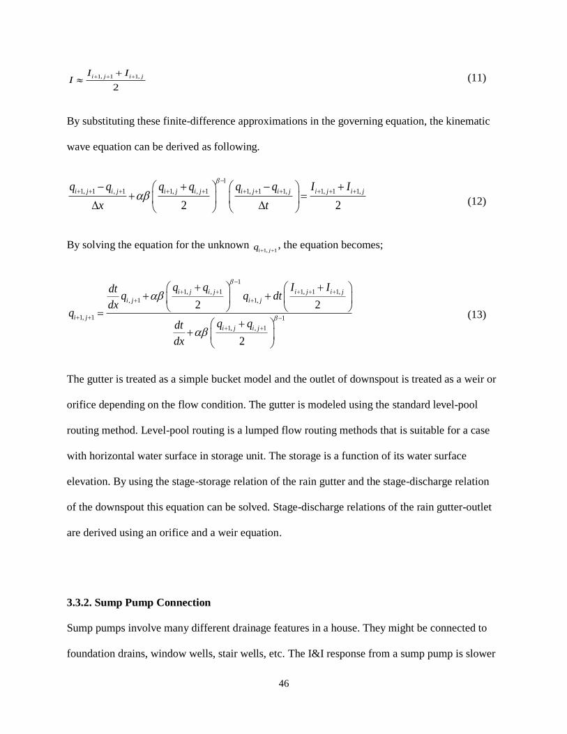
46

1, 1 1,

2

i j i jI II

(11)

By substituting these finite-difference approximations in the governing equation, the kinematic

wave equation can be derived as following.

1, 1 , 1 1, , 1 1, 1 1, 1, 1 1,

2 2

i j i j i j i j i j i j i j i jq q q q q q I I

x t

(12)

By solving the equation for the unknown 1, 1i jq

, the equation becomes;

1

1, , 1 1, 1 1,

, 1 1,

1, 1 1

1, , 1

2 2

2

i j i j i j i j

i j i j

i j

i j i j

q q I Idtq q dt

dxq

q qdt

dx

(13)

The gutter is treated as a simple bucket model and the outlet of downspout is treated as a weir or

orifice depending on the flow condition. The gutter is modeled using the standard level-pool

routing method. Level-pool routing is a lumped flow routing methods that is suitable for a case

with horizontal water surface in storage unit. The storage is a function of its water surface

elevation. By using the stage-storage relation of the rain gutter and the stage-discharge relation

of the downspout this equation can be solved. Stage-discharge relations of the rain gutter-outlet

are derived using an orifice and a weir equation.

3.3.2. Sump Pump Connection

Sump pumps involve many different drainage features in a house. They might be connected to

foundation drains, window wells, stair wells, etc. The I&I response from a sump pump is slower

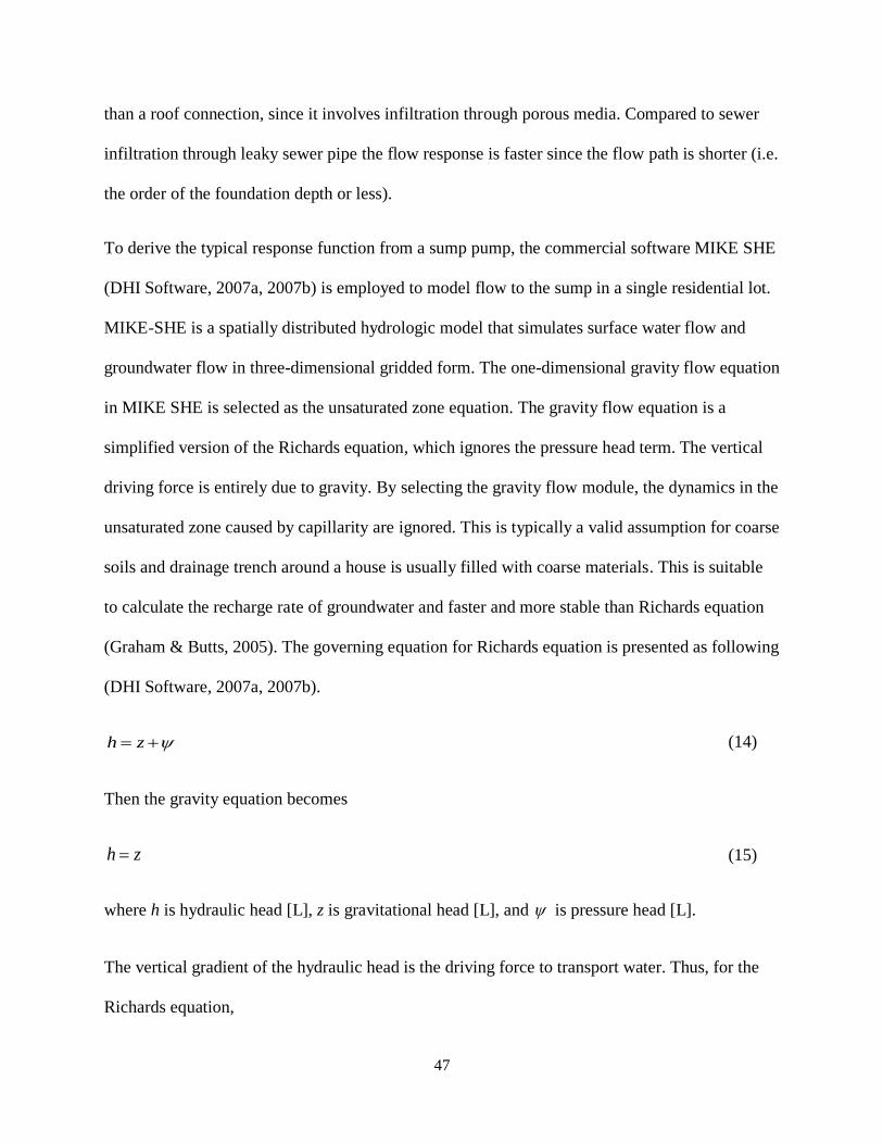
47

than a roof connection, since it involves infiltration through porous media. Compared to sewer

infiltration through leaky sewer pipe the flow response is faster since the flow path is shorter (i.e.

the order of the foundation depth or less).

To derive the typical response function from a sump pump, the commercial software MIKE SHE

(DHI Software, 2007a, 2007b) is employed to model flow to the sump in a single residential lot.

MIKE-SHE is a spatially distributed hydrologic model that simulates surface water flow and

groundwater flow in three-dimensional gridded form. The one-dimensional gravity flow equation

in MIKE SHE is selected as the unsaturated zone equation. The gravity flow equation is a

simplified version of the Richards equation, which ignores the pressure head term. The vertical

driving force is entirely due to gravity. By selecting the gravity flow module, the dynamics in the

unsaturated zone caused by capillarity are ignored. This is typically a valid assumption for coarse

soils and drainage trench around a house is usually filled with coarse materials. This is suitable

to calculate the recharge rate of groundwater and faster and more stable than Richards equation

(Graham & Butts, 2005). The governing equation for Richards equation is presented as following

(DHI Software, 2007a, 2007b).

h z (14)

Then the gravity equation becomes

h z (15)

where h is hydraulic head [L], z is gravitational head [L], and is pressure head [L].

The vertical gradient of the hydraulic head is the driving force to transport water. Thus, for the

Richards equation,

48

hh

z

(16)

and for the gravity equation,

1h

hz

(17)

The volumetric flux that is obtained from Darcy’s law for the gravity equation is

h

q K Kz

(18)

where K is unsaturated hydraulic conductivity [L3/T].

For incompressible soil matrix and soil water with constant density, the continuity equation is:

q

S zt z

(19)

where is volumetric soil moisture [L2] and S is root extraction sink term [L2/T]. The sum of

root extraction over the entire root zone depth is equal to the total actual evapotranspiration.

Direct soil evaporation is computed only in the first node below the surface.

Substituting equation (18) onto equation (19), the following expression is derived.

KS z

t z

(20)

This can be also expressed using the soil water capacity, C

KC S z

t z

(21)

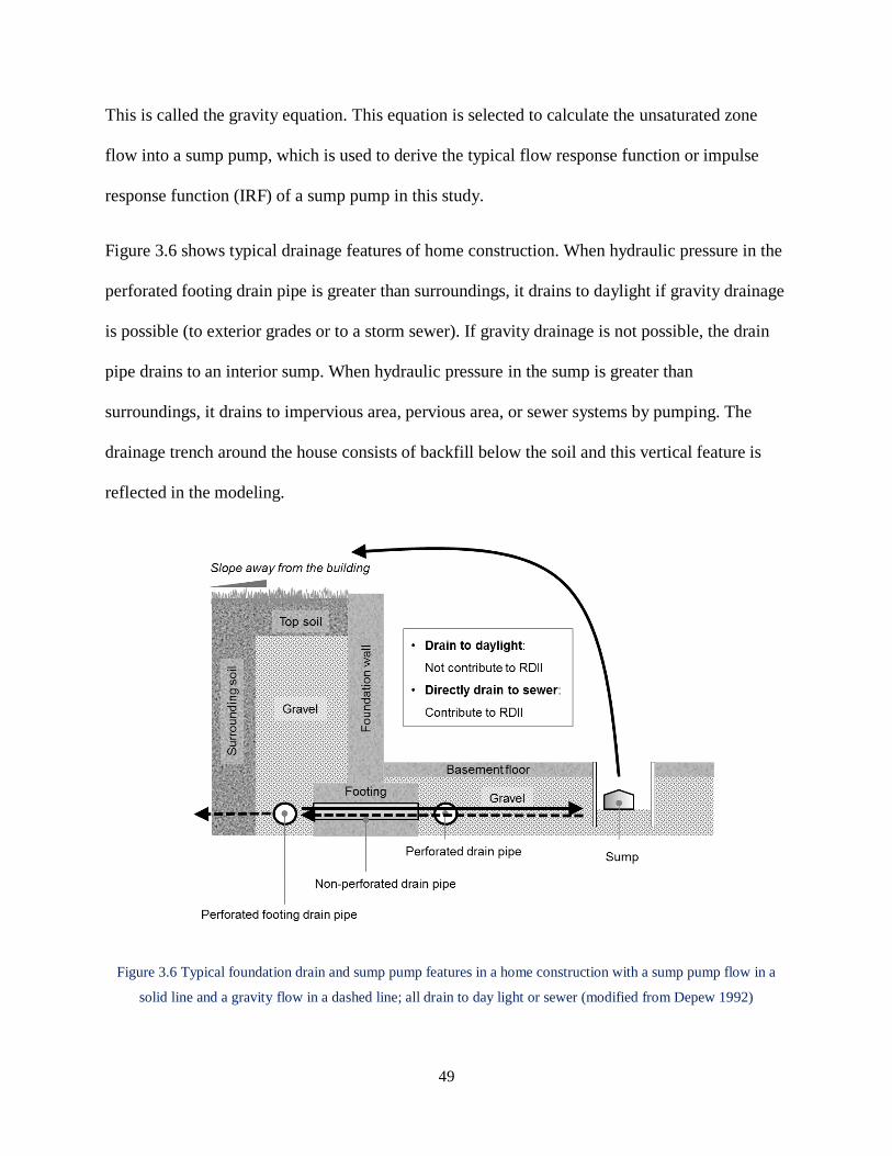
49

This is called the gravity equation. This equation is selected to calculate the unsaturated zone

flow into a sump pump, which is used to derive the typical flow response function or impulse

response function (IRF) of a sump pump in this study.

Figure 3.6 shows typical drainage features of home construction. When hydraulic pressure in the

perforated footing drain pipe is greater than surroundings, it drains to daylight if gravity drainage

is possible (to exterior grades or to a storm sewer). If gravity drainage is not possible, the drain

pipe drains to an interior sump. When hydraulic pressure in the sump is greater than

surroundings, it drains to impervious area, pervious area, or sewer systems by pumping. The

drainage trench around the house consists of backfill below the soil and this vertical feature is

reflected in the modeling.

Figure 3.6 Typical foundation drain and sump pump features in a home construction with a sump pump flow in a

solid line and a gravity flow in a dashed line; all drain to day light or sewer (modified from Depew 1992)

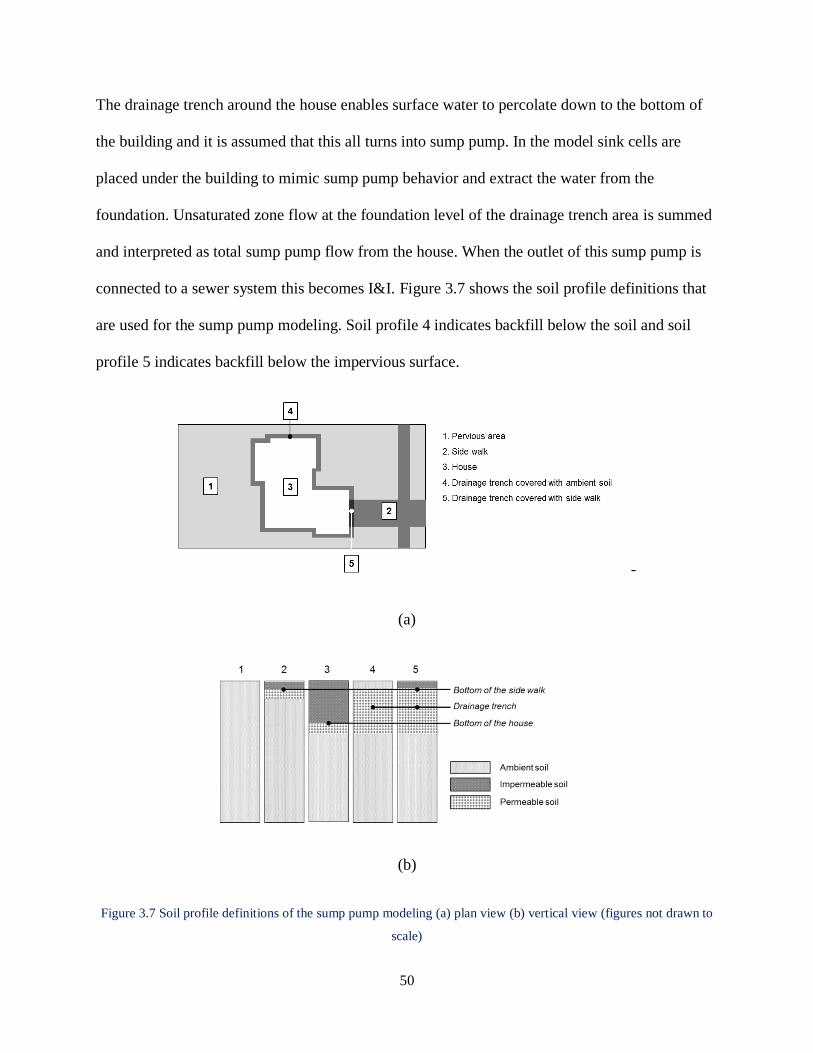
50

The drainage trench around the house enables surface water to percolate down to the bottom of

the building and it is assumed that this all turns into sump pump. In the model sink cells are

placed under the building to mimic sump pump behavior and extract the water from the

foundation. Unsaturated zone flow at the foundation level of the drainage trench area is summed

and interpreted as total sump pump flow from the house. When the outlet of this sump pump is

connected to a sewer system this becomes I&I. Figure 3.7 shows the soil profile definitions that

are used for the sump pump modeling. Soil profile 4 indicates backfill below the soil and soil

profile 5 indicates backfill below the impervious surface.

-

(a)

(b)

Figure 3.7 Soil profile definitions of the sump pump modeling (a) plan view (b) vertical view (figures not drawn to

scale)

51

The size of the domain is 50 m lengthwise and 26 m widthwise. The cell size is 0.33 m x 0.33 m

thus total 150 × 78 or 11700 cells are created. Vertical cell height is 0.2 m. The vegetation was

assumed as uniform grass with Leaf Area Index 5 and Root Depth 100 mm. The width of

drainage trench is assumed as 0.33 m and the total number of cells is 149 which leaves around 50

m length of trench. The drainage trench goes down to the base level of the house, 4 m below the

surface where the sump is located.

Three soil types are employed in the sump pump model: ambient soil, impermeable soil, and

extremely permeable soil. The hydraulic conductivity of the ambient soil is calculated as the

average hydraulic conductivity of soil in Hickory Hills, IL which is the area that the model is

applied to in chapter 4; Kambient = 2.1910-7 m/sec. The soil data from USDA-NRCS soil data mart

are used for the calculation. Hydraulic conductivity of impermeable soil is assumed as 1·10-12

m/sec and 1·100 m/sec is used for extremely permeable soil. The hydraulic conductivity value of

the extremely permeable soil, which represents backfill in the drainage trench is within the range

of the hydraulic conductivity for gravels. Based on Chow et al. (1988), the hydraulic

conductivity for gravels is from 10-1 cm/sec to 102 cm/sec. The Averjanov model (Vogel et al.

2000) is used to simulate a hydraulic conductivity curve that shows the relationship between soil

moisture and hydraulic conductivity.

m

rs

s r

K K

(22)

where Ks is saturated hydraulic conductivity [L/T], s is saturated water content [L3L-3], r is

residual water content [L3L-3], and m is an empirical constant. Following values are used for the

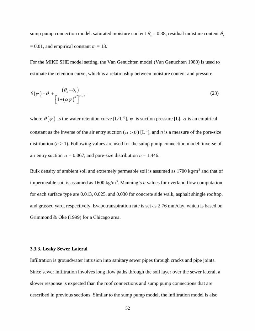
52

sump pump connection model: saturated moisture content s = 0.38, residual moisture content r

= 0.01, and empirical constant m = 13.

For the MIKE SHE model setting, the Van Genuchten model (Van Genuchten 1980) is used to

estimate the retention curve, which is a relationship between moisture content and pressure.

1 1/

1

s r

r nn

(23)

where is the water retention curve [L3L-3], is suction pressure [L], is an empirical

constant as the inverse of the air entry suction ( 0 ) [L-1], and n is a measure of the pore-size

distribution (n > 1). Following values are used for the sump pump connection model: inverse of

air entry suction = 0.067, and pore-size distribution n = 1.446.

Bulk density of ambient soil and extremely permeable soil is assumed as 1700 kg/m3 and that of

impermeable soil is assumed as 1600 kg/m3. Manning’s n values for overland flow computation

for each surface type are 0.013, 0.025, and 0.030 for concrete side walk, asphalt shingle rooftop,

and grassed yard, respectively. Evapotranspiration rate is set as 2.76 mm/day, which is based on

Grimmond & Oke (1999) for a Chicago area.

3.3.3. Leaky Sewer Lateral

Infiltration is groundwater intrusion into sanitary sewer pipes through cracks and pipe joints.

Since sewer infiltration involves long flow paths through the soil layer over the sewer lateral, a

slower response is expected than the roof connections and sump pump connections that are

described in previous sections. Similar to the sump pump model, the infiltration model is also

53

developed using MIKE SHE. The equivalent medium approach from Carlier et al. (2007) is

adopted to simulate the actual flow into the sewer. This simplified approach provided reasonable

results in the flow simulation in agricultural drainage trenches (Carlier et al. 2007). According to

the equivalent medium approach, the leaky sewer pipe and surrounding drainage trench area can

be modeled as a single soil layer with an equivalent uniform hydraulic conductivity. Hydraulic

conductivity of this layer is assumed as 1 m/sec. Soil profile definitions for the leaky sewer pipe

model are presented in Figure 3.8; the leaky sewer lateral is represented as the profile 6 (covered

by ambient soil) and 7 (covered by side walk) depending on the surface types. Infiltrated flow is

estimated as the sum, over the length of the pipe line, of unsaturated flow into the top of the

equivalent porous medium representing the leaky pipe line. The same setting with the sump

pump model in the chapter 3.1.2 was used for the soil type, soil property, Manning’s n values,

and evapotranspiration rate.

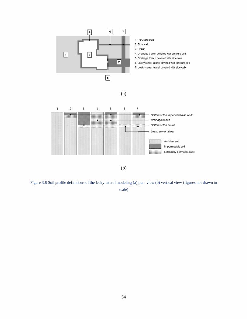
54

(a)

(b)

Figure 3.8 Soil profile definitions of the leaky lateral modeling (a) plan view (b) vertical view (figures not drawn to

scale)

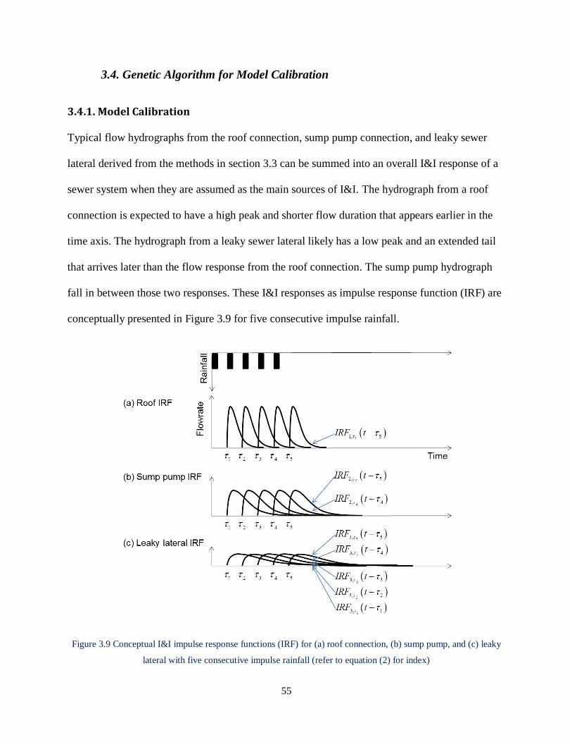
55

3.4. Genetic Algorithm for Model Calibration

3.4.1. Model Calibration

Typical flow hydrographs from the roof connection, sump pump connection, and leaky sewer

lateral derived from the methods in section 3.3 can be summed into an overall I&I response of a

sewer system when they are assumed as the main sources of I&I. The hydrograph from a roof

connection is expected to have a high peak and shorter flow duration that appears earlier in the

time axis. The hydrograph from a leaky sewer lateral likely has a low peak and an extended tail

that arrives later than the flow response from the roof connection. The sump pump hydrograph

fall in between those two responses. These I&I responses as impulse response function (IRF) are

conceptually presented in Figure 3.9 for five consecutive impulse rainfall.

Figure 3.9 Conceptual I&I impulse response functions (IRF) for (a) roof connection, (b) sump pump, and (c) leaky

lateral with five consecutive impulse rainfall (refer to equation (2) for index)

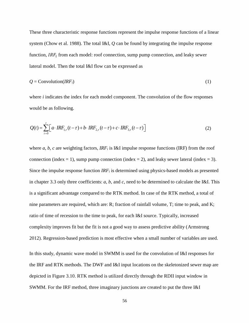
56

These three characteristic response functions represent the impulse response functions of a linear

system (Chow et al. 1988). The total I&I, Q can be found by integrating the impulse response

function, 𝐼𝑅𝐹𝑖 from each model: roof connection, sump pump connection, and leaky sewer

lateral model. Then the total I&I flow can be expressed as

Q = Convolution(IRFi) (1)

where i indicates the index for each model component. The convolution of the flow responses

would be as following.

1, 2, 3,

0

( ) ( ) ( ) ( )t

Q t a IRF t b IRF t c IRF t

(2)

where a, b, c are weighting factors, IRFi is I&I impulse response functions (IRF) from the roof

connection (index = 1), sump pump connection (index = 2), and leaky sewer lateral (index = 3).

Since the impulse response function IRFi is determined using physics-based models as presented

in chapter 3.3 only three coefficients: a, b, and c, need to be determined to calculate the I&I. This

is a significant advantage compared to the RTK method. In case of the RTK method, a total of

nine parameters are required, which are: R; fraction of rainfall volume, T; time to peak, and K;

ratio of time of recession to the time to peak, for each I&I source. Typically, increased

complexity improves fit but the fit is not a good way to assess predictive ability (Armstrong

2012). Regression-based prediction is most effective when a small number of variables are used.

In this study, dynamic wave model in SWMM is used for the convolution of I&I responses for

the IRF and RTK methods. The DWF and I&I input locations on the skeletonized sewer map are

depicted in Figure 3.10. RTK method is utilized directly through the RDII input window in

SWMM. For the IRF method, three imaginary junctions are created to put the three I&I

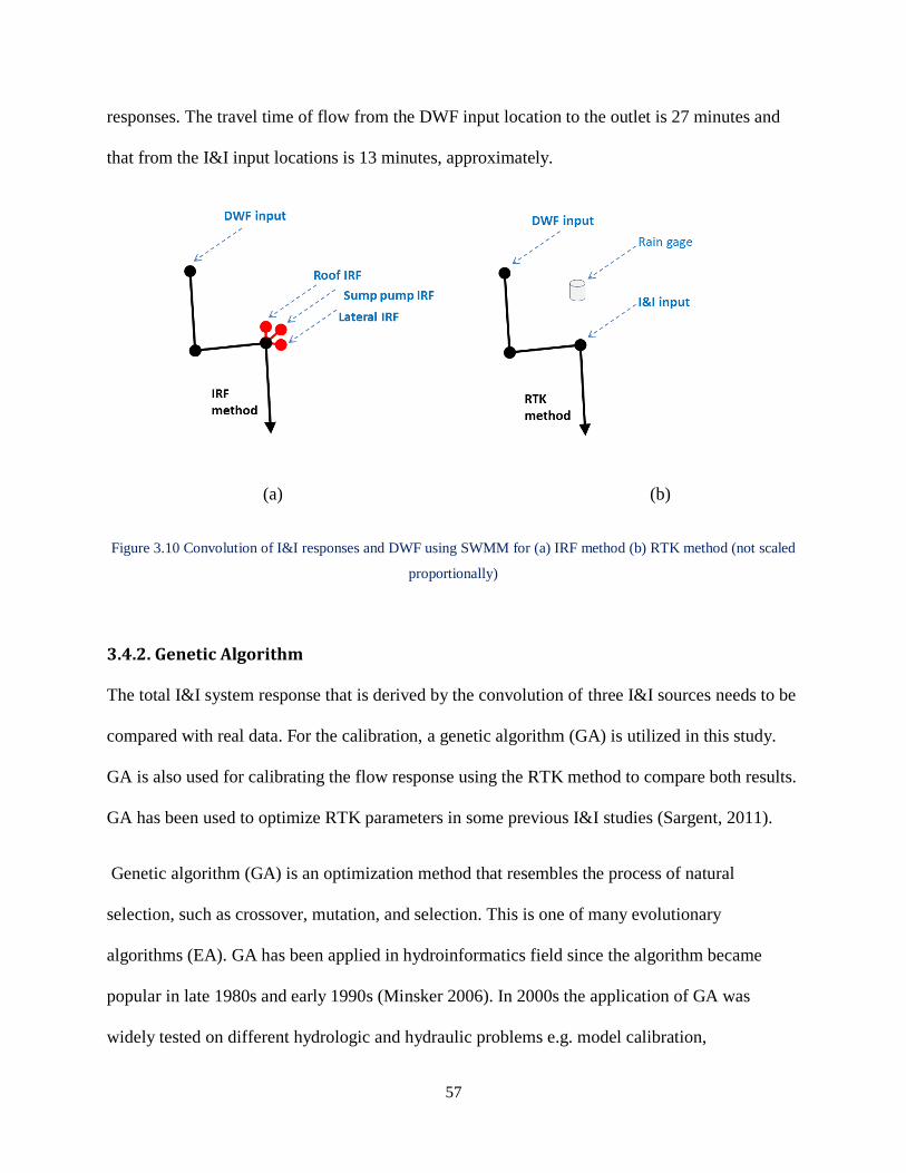
57

responses. The travel time of flow from the DWF input location to the outlet is 27 minutes and

that from the I&I input locations is 13 minutes, approximately.

(a) (b)

Figure 3.10 Convolution of I&I responses and DWF using SWMM for (a) IRF method (b) RTK method (not scaled

proportionally)

3.4.2. Genetic Algorithm

The total I&I system response that is derived by the convolution of three I&I sources needs to be

compared with real data. For the calibration, a genetic algorithm (GA) is utilized in this study.

GA is also used for calibrating the flow response using the RTK method to compare both results.

GA has been used to optimize RTK parameters in some previous I&I studies (Sargent, 2011).

Genetic algorithm (GA) is an optimization method that resembles the process of natural

selection, such as crossover, mutation, and selection. This is one of many evolutionary

algorithms (EA). GA has been applied in hydroinformatics field since the algorithm became

popular in late 1980s and early 1990s (Minsker 2006). In 2000s the application of GA was

widely tested on different hydrologic and hydraulic problems e.g. model calibration,

58

groundwater monitoring and remediation design, watershed, reservoir, and river management,

and water distribution system design. Zimmer et al. (2010) applied GA to real-time combined

sewer overflow (CSO) control. In the commercial sector, Innovyze provides GA optimization

tools to calibrate the RTK parameters in H2OMap SWMM and InfoSWMM.

The algorithm starts with a random population, which are sets of suitable parameters, or genes,

for the problem. These parameter sets are called chromosomes. Then the fitness of the model

solutions using these chromosomes is tested for selection. Chromosomes from one population

are used to generate a new population and the offsprings in the new population are hoped to be

better than the old ones. The new population is created by repeating following steps.

Selection: Two parent chromosomes are selected on the basis of fitness. The probability

of individuals is higher when the fitness of the individual is greater than its competiter’s

fitness. If the parents have better fitness, there is a greater chance to be selected.

Crossover: With the user-defined crossover probability, a new offspring is formed by

crossover the chromosomes from both parents.

Mutation: With the user-defined mutation probability, new offspring is mutated at each

position in chromosomes. Mutation allows one or more gene values in a chromosome

altered from its initial state. This maintains diversity in the solutions that lead to the

algorithm searching a wider space for optimal solutions.

Accepting: New offspring is placed in a new population.

This process is repeated until the solution converges and the error of fitness is minimized.

Offsprings with better fitness have more chances to reproduce. Selection and crossover are the

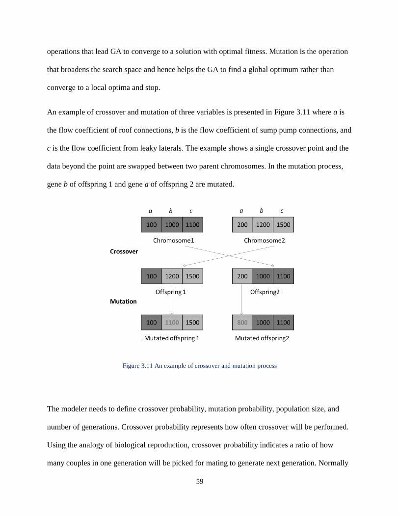
59

operations that lead GA to converge to a solution with optimal fitness. Mutation is the operation

that broadens the search space and hence helps the GA to find a global optimum rather than

converge to a local optima and stop.

An example of crossover and mutation of three variables is presented in Figure 3.11 where a is

the flow coefficient of roof connections, b is the flow coefficient of sump pump connections, and

c is the flow coefficient from leaky laterals. The example shows a single crossover point and the

data beyond the point are swapped between two parent chromosomes. In the mutation process,

gene b of offspring 1 and gene a of offspring 2 are mutated.

Figure 3.11 An example of crossover and mutation process

The modeler needs to define crossover probability, mutation probability, population size, and

number of generations. Crossover probability represents how often crossover will be performed.

Using the analogy of biological reproduction, crossover probability indicates a ratio of how

many couples in one generation will be picked for mating to generate next generation. Normally

60

it is good to leave some parts of population survive to next generation and the selection of

parents is made based on fitness. When memory is allowed, the best chromosomes are preserved

into next generation. Mutation probability is how often parts of chromosome will be mutated.

Mutation probability should be small since GA will behave like a random search with high

mutation probability. Population size means how many chromosomes are in the population in

one generation. With a small population size only small part of search space is explored and one

may only find a local solution. With a large population size GA takes longer to run. After some

limit, increased population size is found not to be too useful (Minsker 2006).

61

References

Allitt, R. (2002) Rainfall, runoff and infiltration re-visited. WaPUG Spring Meeting 2002 (pp. 1–

9).

Armstrong, J. S. (2012) Illusions in regression analysis. International Journal of Forecasting.

Backmeyer, D. P. (1960) Effects of infiltration. Water Pollution Control Federation 32(5), 539–

540.




Buyuktas, D. & Wallender, W. W. (2002) Numerical simulation of water flow and solute

transport to tile drains. Journal of Irrigation and Drainage Engineering 128(1), 49–56.

Camp Dresser & McKee (CDM) Inc., F.E. Jordan Associates Inc. & James M. Montgomery

Consulting Engineers. (1985) East Bay infiltration/inflow study manual for cost-

effectiveness analysis. Oakland, CA.

Carlier, J. P., Kao, C. & Ginzburg, I. (2007) Field-scale modeling of subsurface tile-drained soils

using an equivalent-medium approach. Journal of Hydrology 341(1-2), 105–115.

doi:10.1016/j.jhydrol.2007.05.006

Carluer, N. & Marsily, G. De. (2004) Assessment and modelling of the influence of man-made

networks on the hydrology of a small watershed: implications for fast flow components,

62

water quality and landscape management. Journal of Hydrology 285(1-4), 76–95.

doi:10.1016/j.jhydrol.2003.08.008

Chow, V. Te, Maidment, D. R., & Mays, L. W. (1988) Applied Hydrology (pp. 110–115).

McGraw-Hill.

Cooke, R. A. & Badiger, S. (2001) Drainage equations for random and irregular tile drainage

systems. Agricultural Water Management 48, 207–224.

Crawford, D., Eckley, P. & Pier, E. (1999) Methods for estimating inflow and infiltration into

sanitary sewers. New applications in modeling urban water systems, Volume 7, Conference

on Stormwater and Related Water Systems Modeling; Management and Impacts, 299–315.

Toronto: CHI.

De Bénédittis, J. & Bertrand-Krajewski, J. L. (2005) Infiltration in sewer systems: comparison of

measurement methods. Water Science and Technology: a Journal of the International



Depew, N. (2007, November 25) Drainage 101, Part I. Ned Depew House Inspection. Retrieved

March 27, 2014, from http://www.buyershouseinspection.com/HC/HC2.html.

DHI Software. (2007) MIKE SHE user manual volume 1: user guide (Vol. 1).

DHI Software. (2007) MIKE SHE user manual volume 2: reference guide (Vol. 2).

63

Ertl, T. W., Dlauhy, F. & Haberl, R. (2002) Investigations of the amount of infiltration / inflow

into a sewage system. Proceedings of the 3rd “Sewer Processes and Networks”


Fipps, G., Skaggs, R. W., & Nieber, J. L. (1986) Drains as a boundary condition in finite

elements. Water Resources Research, 22(11), 1613–1621.

Fipps, G., & Skaggs, R. W. (1992) Simple methods for predicting flow to drains. Journal of

Irrigation and Drainage Engineering, 117(6), 881–896.



Golden, J. B. (1995) An introduction to sanitary sewer overflows. In Seminar publication:

National conference on sanitary sewer overflows (SSOs) (pp. 443–450). Washington D.C.:

EPA.


Gustafsson, L. (2000) Alternative drainage schemes for reduction of inflow/infiltration -

prediction and follow-up of effects with the aid of an integrated sewer/aquifer model. 1st

International Conference on Urban Drainage via Internet (pp. 21–37).

Innovyze. (2011) InfoWorks CS technical review.

Jardin, N. (2004) Fremdwasser – eine grundsätzliche Problembeschreibung (Extraneous water –

a basic description). Proceedings of 3rd Forum Ruhrverband. Essen, Germany.

64




Kim, S., & Delleur, J. W. (1997) Sensitivity analysis of extended TOPMODEL for agricultural

watersheds equipped with tile drains. Hydrological Processes, 11, 1243–1261.




Lai, F. D. (2008) Review of sewer design criteria and RDII prediction methods. Washington,

DC.

Lindberg, S., Nielsen, J. B., & Carr, R. (1989) An integrated PC-modelling system for hydraulic

analysis of drainage systems. Watercomp ’89: The First Australasian Conference on

Technical Computing in the Water Industry. Melbourne, Australia.

Lucas, S. (2003) Auftreten, Ursachen und Auswirkungen hoher Fremdwasserabflüsse – eine

zeitliche und räumliche nalyse (Occurence, causes and effects of high extraneous water

flows). Universität Karlsruhe.

Minsker, B. (2006) Genetic algorithm. In P. Kumar, J. C. Alameda, P. Bajcsy, M. Folk, & M.

Markus (Eds.), Hydroinformatics: Data integrative approaches in computation, analysis,

and modeling (pp. 437–451). CRC Press.

65

NCPWI (National Council on Public Works Improvement). (1988) Fragile foundations: a report

on America’s Public Works, Final report to the president and congress.

NSFC (National Small Flows Clearinghouse). (1999) Infiltration and inflow can be costly for

communities. Pipeline: Small Community Wastewater Issues Explained to the Public,

Vol.10, No.2.

Pawlowski, C. W., Rhea, L., Shuster, W. D., & Barden, G. (2013) Some factors affecting inflow

and infiltration from residential sources in a core urban area: A case study in a Columbus

OH USA neighborhood. Journal of Hydraulic Engineering. doi:10.1061/(ASCE)HY.1943-

7900.0000799

Pecher, K. H. (2003) Fremdwasseranfall, Schwankungen und Konsequenzen für die

Abwasserbehandlung (Amount of I/I, variations and consequences). Proceedings of 36th

Essener Tagung, Gewässerschutz-Wasser-Abwasser. Aachen, Germany.

Peters, G. L., & Troemper, A. P. (1969) Reduction of hydraulic sewer loading by downspout

removal. Water Pollution Control Federation, 41(1), 63–81.

Petroff, R. G. (1996) An analysis of the root cause of sanitary sewer overflows. In: Seminar

Publication National Conference on Sanitary Sewer Overflows (SSOs): april 24-26, 1995,

Washington D.C., 8–15. Cincinnati, OH: EPA.

Purkey, D. R., Wallender, W. W., Fogg, G. E. & Sivakumar, B. (2004) Describing near surface,

transient flow processes in unconfined aquifers below irrigated lands: Model application in

66

the Western San Joaquin Valley, California. Journal of Irrigation and Drainage

Engineering 130(6), 451–459. doi:10.1061/(ASCE)0733-9437(2004)130

Qiao, F., Lu, H., Derr, H. K., Wang, M., & Chen, M. (2007) A new method of predicting rainfall

dependent inflow and infiltration. Water Environment Federation (pp. 1883–1890).

doi:10.2175/193864707788116040

Reynolds, J. (1995) The roof drain and sump pump removal program: An innovative approach to

inflow reduction. In Seminar publication: National conference on sanitary sewer overflows

(SSOs) (pp. 303–309). Washington D.C.: EPA.

Rossman, L. A. (2010) Storm water management model user’s manual version 5.0. Cincinnati,

OH.

Sargent, S. W. (2011) How often will sewage spill?: Stochastic analysis & design of a waste-

water system with large RDII components. In Water New Zealand (pp. 1–28).

Schulz, N., Baur, R., & Krebs, P. (2005) Integrated modelling for the evaluation of infiltration

effects. Water science and technology: a journal of the International Association on Water

Pollution Research, 52(5), 215–23. Retrieved from


Seo, Y. (2012) The effect of rainstorm movement on urban drainage network runoff

hydrographs. University of Illinois at Urbana-Champaign.

Seo, Y., & Schmidt, A. R. (2012) The effect of rainstorm movement on urban drainage network

runoff hydrographs. Hydrological Processes, 26(25), 3830–3841. doi:10.1002/hyp.8412

67

Seo, Y., Schmidt, A. R., & Sivapalan, M. (2012) Effect of storm movement on flood peaks:

Analysis framework based on characteristic timescales. Water Resources Research, 48(5),

n/a–n/a. doi:10.1029/2011WR011761

Sliter, J. T. (1974) Infiltration/inflow guidelines spark controversy. Journal of Water Pollution

Control Federation, 46(1), 6–8.

Strand Associates Inc. (2006) Inflow and Iifiltration from private property. Cincinnati, OH.

Tarboton, K. C. & Wallender, W. W. (2000) Finite-element grid configurations for drains.

Journal of Irrigation and Drainage Engineering 126(4), 243–249.

Vallabhaneni, S., Chan, C. C., & Burgess, E. H. (2007) Computer tools for sanitary sewer system

capacity analysis and planning. Cincinnati, OH.

Vallabhaneni, S., Lai, F., Chan, C., Burgess, E. H. & Field, R. (2008) SSOAP − A USEPA

toolbox for sanitary sewer overflow analysis and control planning. EWRI 2008 World

Environmental & Water Resources Congress, May 13-16, 2008. Honolulu, HI: American

Society of Civil Engineers (ASCE).

Van Genuchten, M. T. (1980) A closed-form equation for predicting the hydraulic conductivity

of unsaturated soils. Soil Science Society of America, 44(5), 892–898.

Vogel, T., Van Genuchten, M. T., & Cislerova, M. (2000) Effect of the shape of the soil

hydraulic functions near saturation on variably-saturated low predictions. Advances In

Water Resources, 24, 133–144.

68

Weiss, G., Brombach, H. & Haller, B. (2002) Infiltration and inflow in combined sewer

systems: long-term analysis. Water science and technology: a journal of the International



Wright, L., Dent, S., Mosley, C., Kadota, P. & Djebbar, Y. (2001) Comparing rainfall dependent

inflow and infiltration simulation method. In: Models and Applications to Urban Water

Systems. Monograph 9, 235–258. Toronto, Ontario, Canada: CHI.

Zimmer, A., Minsker, B., Schmidt, A., & Ostfeld, A. (2010) Evolutionary Algorithm Memory

Enhancement for Real-Time CSO Control. In World Environmental and Water Resources

Congress (pp. 2251–2259). Providence, Rhode Island.

69

4. I&I Response Functions

4.1. Typical I&I Response Functions

In this section, three I&I response functions of a roof downspout connection, sump pump

connection, and leaky lateral are presented using the physics-based models introduced in chapter

3. The impulse response functions (IRF) from three sources show distinguishable differences in

response time and peak flowrates. This makes applying Genetic Algorithm (GA) suitable for the

IRF integration and the model calibration.

The three IRFs are identified for the study area Hickory Hills, IL where sewer drainage

configurations and sewer flow monitoring data are available. Hickory Hills is a city in Cook

County, IL with the size of 7.33 km2 and the population of 14,049 (U.S. Census Bureau 2010).

The climate of the city is classified as humid continental (Köppen Dfa) and the average rainfall is

approximately 98 cm per year (Hickory Hills (zip 60457), Illinois Climate 2014).

4.1.1. Uniform rainfall

To derive typical I&I responses from the three models, a representative uniform rainfall was

introduced. From January 1, 2009 to July 31, 2009, a total of 702 mm of rainfall was recorded in

Hickory Hills, IL. Seventeen distinct storm events were identified during this period; hence the

average rainfall volume for a single event is 41 mm. The maximum rainfall intensity during the

period is 14 mm/hr. Three hours of 14 mm/hr of rainfall produces a total of 42 mm of rainfall

volume. Therefore, 3 hour 14 mm/hr uniform rainfall is selected as a representative storm event

for the investigation in this section (Figure 4.1). In chapter 5, sensitivity of model for different

rainfall distribution is addressed in addition to the 42 mm uniform rainfall.

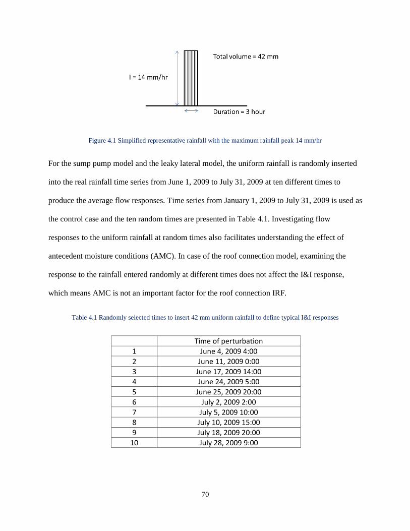
70

Figure 4.1 Simplified representative rainfall with the maximum rainfall peak 14 mm/hr

For the sump pump model and the leaky lateral model, the uniform rainfall is randomly inserted

into the real rainfall time series from June 1, 2009 to July 31, 2009 at ten different times to

produce the average flow responses. Time series from January 1, 2009 to July 31, 2009 is used as

the control case and the ten random times are presented in Table 4.1. Investigating flow

responses to the uniform rainfall at random times also facilitates understanding the effect of

antecedent moisture conditions (AMC). In case of the roof connection model, examining the

response to the rainfall entered randomly at different times does not affect the I&I response,

which means AMC is not an important factor for the roof connection IRF.

Table 4.1 Randomly selected times to insert 42 mm uniform rainfall to define typical I&I responses

Time of perturbation

1 June 4, 2009 4:00

2 June 11, 2009 0:00

3 June 17, 2009 14:00 4 June 24, 2009 5:00

5 June 25, 2009 20:00

6 July 2, 2009 2:00

7 July 5, 2009 10:00 8 July 10, 2009 15:00

9 July 18, 2009 20:00

10 July 28, 2009 9:00

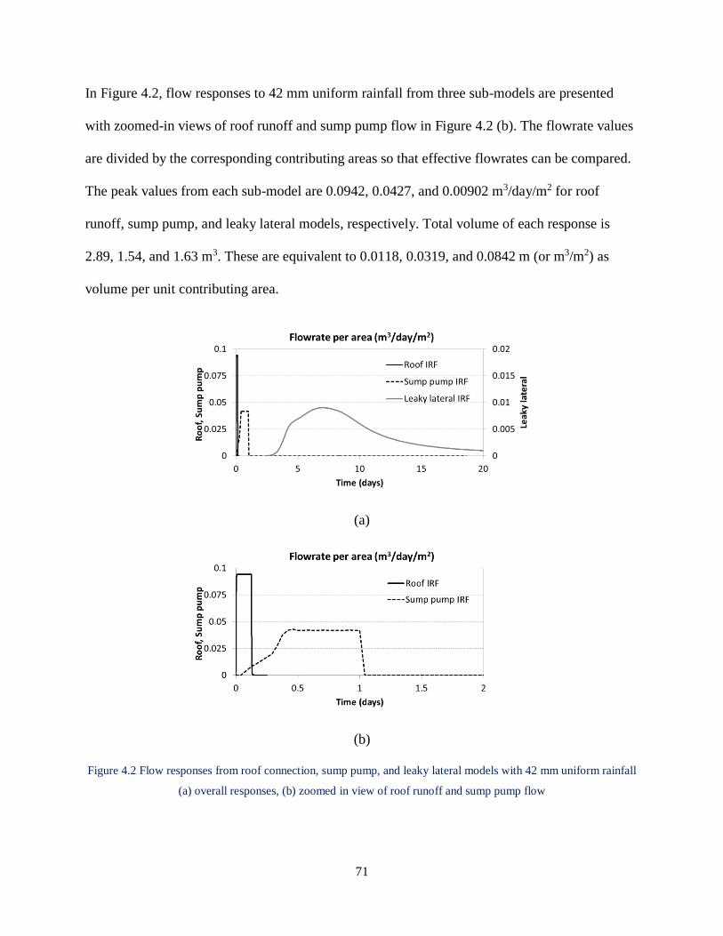
71

In Figure 4.2, flow responses to 42 mm uniform rainfall from three sub-models are presented

with zoomed-in views of roof runoff and sump pump flow in Figure 4.2 (b). The flowrate values

are divided by the corresponding contributing areas so that effective flowrates can be compared.

The peak values from each sub-model are 0.0942, 0.0427, and 0.00902 m3/day/m2 for roof

runoff, sump pump, and leaky lateral models, respectively. Total volume of each response is

2.89, 1.54, and 1.63 m3. These are equivalent to 0.0118, 0.0319, and 0.0842 m (or m3/m2) as

volume per unit contributing area.

(a)

(b)

Figure 4.2 Flow responses from roof connection, sump pump, and leaky lateral models with 42 mm uniform rainfall

(a) overall responses, (b) zoomed in view of roof runoff and sump pump flow

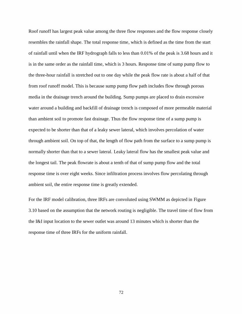
72

Roof runoff has largest peak value among the three flow responses and the flow response closely

resembles the rainfall shape. The total response time, which is defined as the time from the start

of rainfall until when the IRF hydrograph falls to less than 0.01% of the peak is 3.68 hours and it

is in the same order as the rainfall time, which is 3 hours. Response time of sump pump flow to

the three-hour rainfall is stretched out to one day while the peak flow rate is about a half of that

from roof runoff model. This is because sump pump flow path includes flow through porous

media in the drainage trench around the building. Sump pumps are placed to drain excessive

water around a building and backfill of drainage trench is composed of more permeable material

than ambient soil to promote fast drainage. Thus the flow response time of a sump pump is

expected to be shorter than that of a leaky sewer lateral, which involves percolation of water

through ambient soil. On top of that, the length of flow path from the surface to a sump pump is

normally shorter than that to a sewer lateral. Leaky lateral flow has the smallest peak value and

the longest tail. The peak flowrate is about a tenth of that of sump pump flow and the total

response time is over eight weeks. Since infiltration process involves flow percolating through

ambient soil, the entire response time is greatly extended.

For the IRF model calibration, three IRFs are convoluted using SWMM as depicted in Figure

3.10 based on the assumption that the network routing is negligible. The travel time of flow from

the I&I input location to the sewer outlet was around 13 minutes which is shorter than the

response time of three IRFs for the uniform rainfall.

73

4.1.2. Real rainfall

Using the three I&I IRF of the representative unit rainfall, flow responses of three I&I sources—

roof drain, sump pump, and leaky lateral—are derived for the real rainfall data from Hickory

Hills, IL from April 17, 2009 to July 16, 2009. The total rainfall depth for this period is 372 mm

and the peak precipitation rate is 13 mm/hr (Figure 4.3 (a)). The three I&I flow responses are

presented in Figure 4.3 (b) with a zoomed-in view for the shorter period, from June 16 to July 3,

in Figure 4.3 (c). To compare the net I&I per area, the flow is divided by the effective

contributing area of each model: area of roof 246 m2, area of drainage trench around the building

48 m2, and area of leaky lateral layer 19 m2. The effective contributing area assumes that lateral

subsurface flow is negligible relative to vertical flow. The flow per unit area is only used for

comparison in Figure 4.3; when IRF is used for calibration flow is not scaled per unit area.

In Figure 4.3 (b), the roof response is depicted by a black solid line, the sump pump response as

by a black dashed line, and the lateral response as by a grey solid line. The time of roof response

peaks match well with that of the rainfall peaks. Similar to the representative uniform rainfall

responses, peaks of the sump pump and lateral responses show delays.

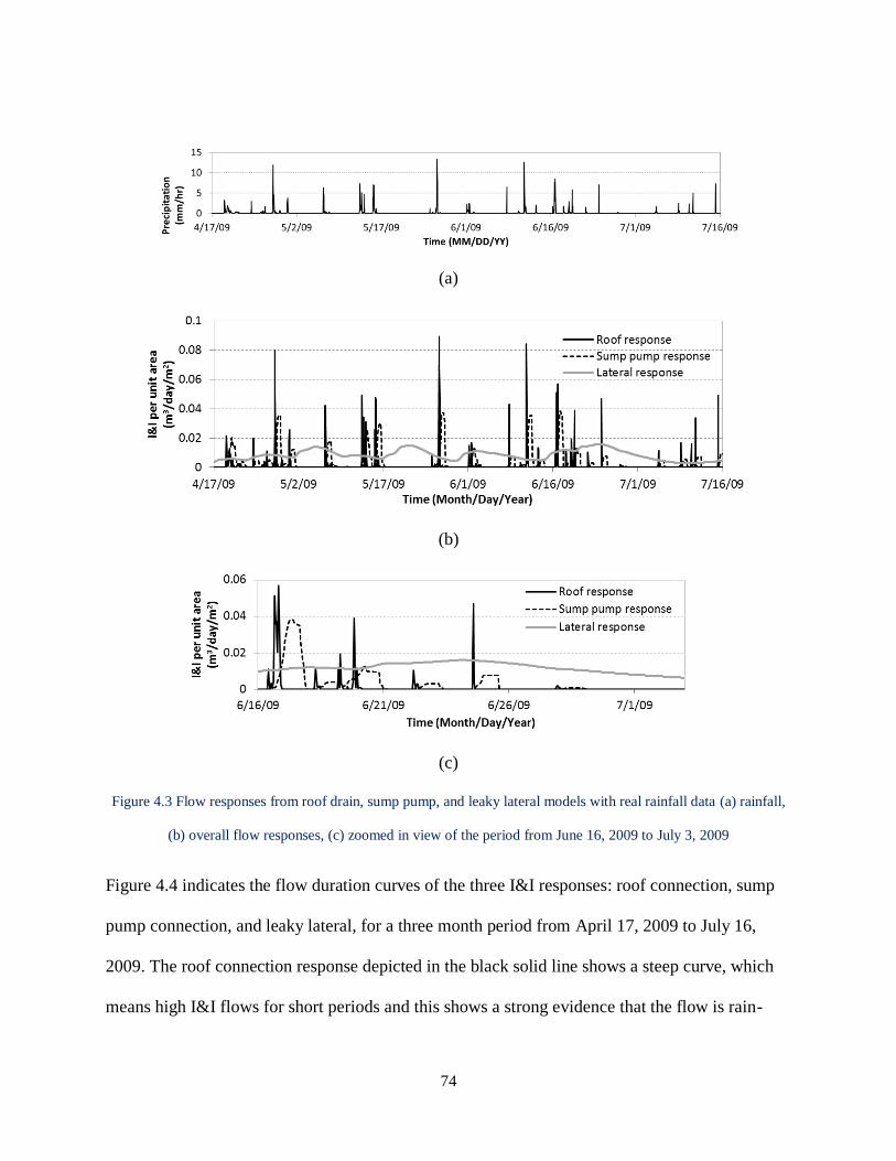
74

(a)

(b)

(c)

Figure 4.3 Flow responses from roof drain, sump pump, and leaky lateral models with real rainfall data (a) rainfall,

(b) overall flow responses, (c) zoomed in view of the period from June 16, 2009 to July 3, 2009

Figure 4.4 indicates the flow duration curves of the three I&I responses: roof connection, sump

pump connection, and leaky lateral, for a three month period from April 17, 2009 to July 16,

2009. The roof connection response depicted in the black solid line shows a steep curve, which

means high I&I flows for short periods and this shows a strong evidence that the flow is rain-

75

caused. The leaky lateral response, which is presented by a grey solid line, shows a flatter curve.

This indicates that the infiltration through leaky laterals is sustained longer than the hourly time

scale due to the flow through porous media; ambient soil on top of a more permeable layer

surrounding the leaky pipe. The sump pump response in the black dashed line falls between the

roof connection and the leaky lateral response curves. The sump pump response involves a flow

through a porous media like the leaky lateral response but the flow distance in an ambient soil,

which has a small hydraulic conductivity, is shorter.

The shapes of the three curves are very different, which provides insight into the very different

processes. Roof connection flow duration curve is very steep and indicates that approximately

90% of flow values are nearly zero. Sump pump flow duration curve is also very steep and

indicates that approximately 75% of the flows are nearly zero. However, the sump pump curve

flattens out at around the exceedance probability 0.05. The model to generate the sump pump

IRF considers both the flow into the sump and the capacity of the sump pump and limits the IRF

flow to the smaller of these values. The flat flow-duration for the extreme events indicates the

storms for which the sump pump capacity limits the flow. The flow duration curve of leaky

lateral never hits zero. Peaks never get as high as those from the roof and sump but there is

always some flow even though it is small.

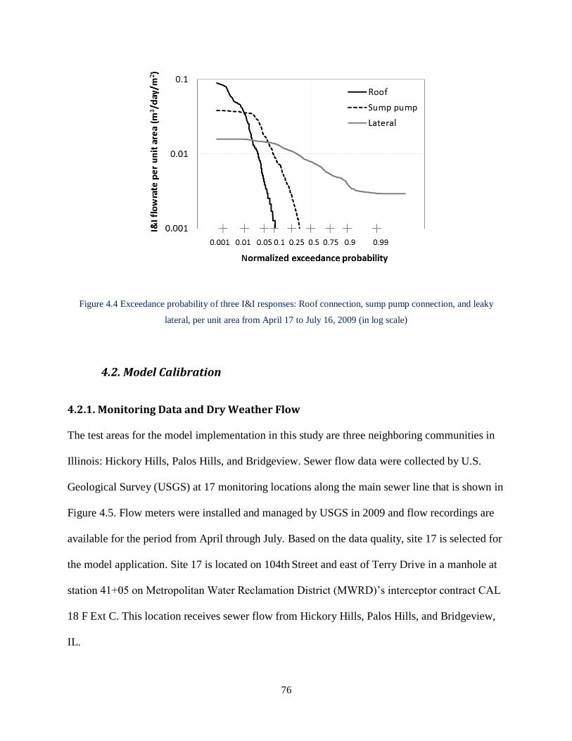
76

Figure 4.4 Exceedance probability of three I&I responses: Roof connection, sump pump connection, and leaky

lateral, per unit area from April 17 to July 16, 2009 (in log scale)

4.2. Model Calibration

4.2.1. Monitoring Data and Dry Weather Flow

The test areas for the model implementation in this study are three neighboring communities in

Illinois: Hickory Hills, Palos Hills, and Bridgeview. Sewer flow data were collected by U.S.

Geological Survey (USGS) at 17 monitoring locations along the main sewer line that is shown in

Figure 4.5. Flow meters were installed and managed by USGS in 2009 and flow recordings are

available for the period from April through July. Based on the data quality, site 17 is selected for

the model application. Site 17 is located on 104th Street and east of Terry Drive in a manhole at

station 41+05 on Metropolitan Water Reclamation District (MWRD)’s interceptor contract CAL

18 F Ext C. This location receives sewer flow from Hickory Hills, Palos Hills, and Bridgeview,

IL.

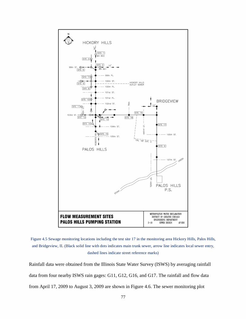
77

Figure 4.5 Sewage monitoring locations including the test site 17 in the monitoring area Hickory Hills, Palos Hills,

and Bridgeview, IL (Black solid line with dots indicates main trunk sewer, arrow line indicates local sewer entry,

dashed lines indicate street reference marks)

Rainfall data were obtained from the Illinois State Water Survey (ISWS) by averaging rainfall

data from four nearby ISWS rain gages: G11, G12, G16, and G17. The rainfall and flow data

from April 17, 2009 to August 3, 2009 are shown in Figure 4.6. The sewer monitoring plot

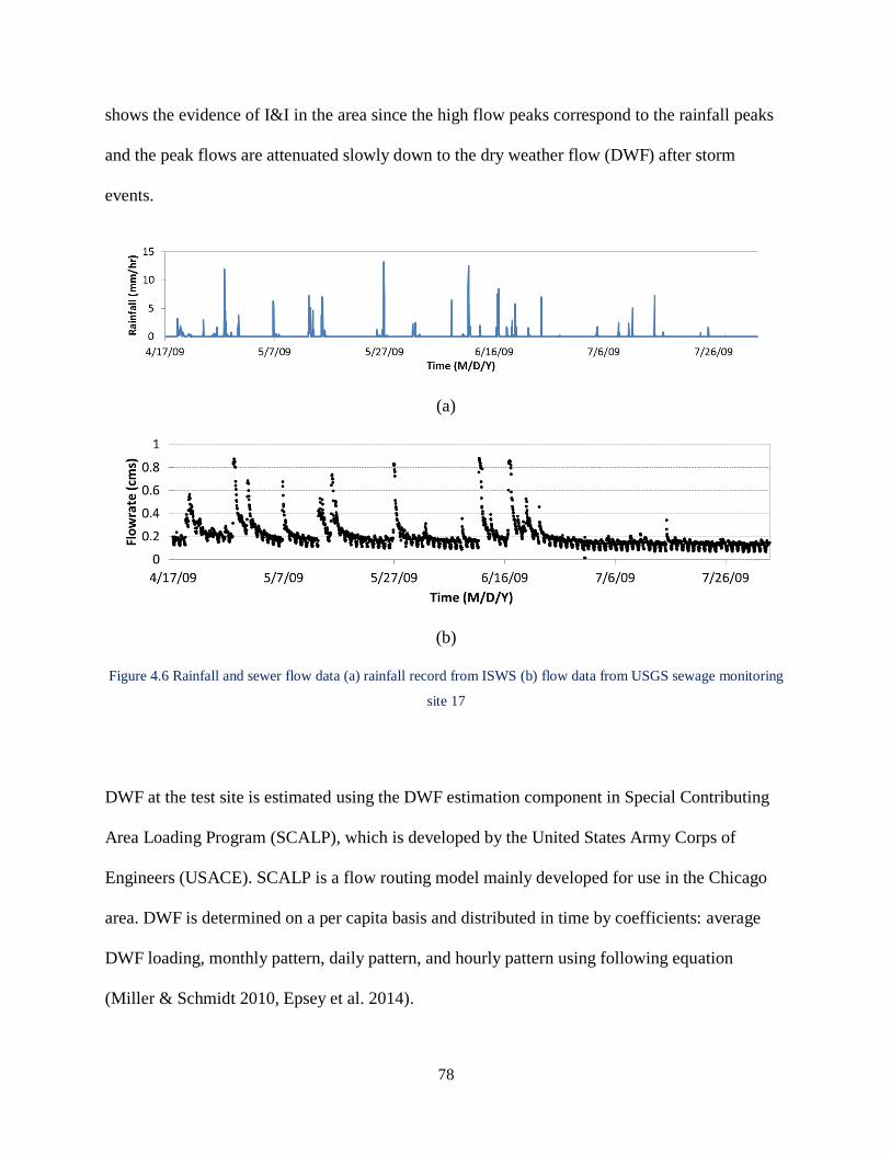
78

shows the evidence of I&I in the area since the high flow peaks correspond to the rainfall peaks

and the peak flows are attenuated slowly down to the dry weather flow (DWF) after storm

events.

(a)

(b)

Figure 4.6 Rainfall and sewer flow data (a) rainfall record from ISWS (b) flow data from USGS sewage monitoring

site 17

DWF at the test site is estimated using the DWF estimation component in Special Contributing

Area Loading Program (SCALP), which is developed by the United States Army Corps of

Engineers (USACE). SCALP is a flow routing model mainly developed for use in the Chicago

area. DWF is determined on a per capita basis and distributed in time by coefficients: average

DWF loading, monthly pattern, daily pattern, and hourly pattern using following equation

(Miller & Schmidt 2010, Epsey et al. 2014).

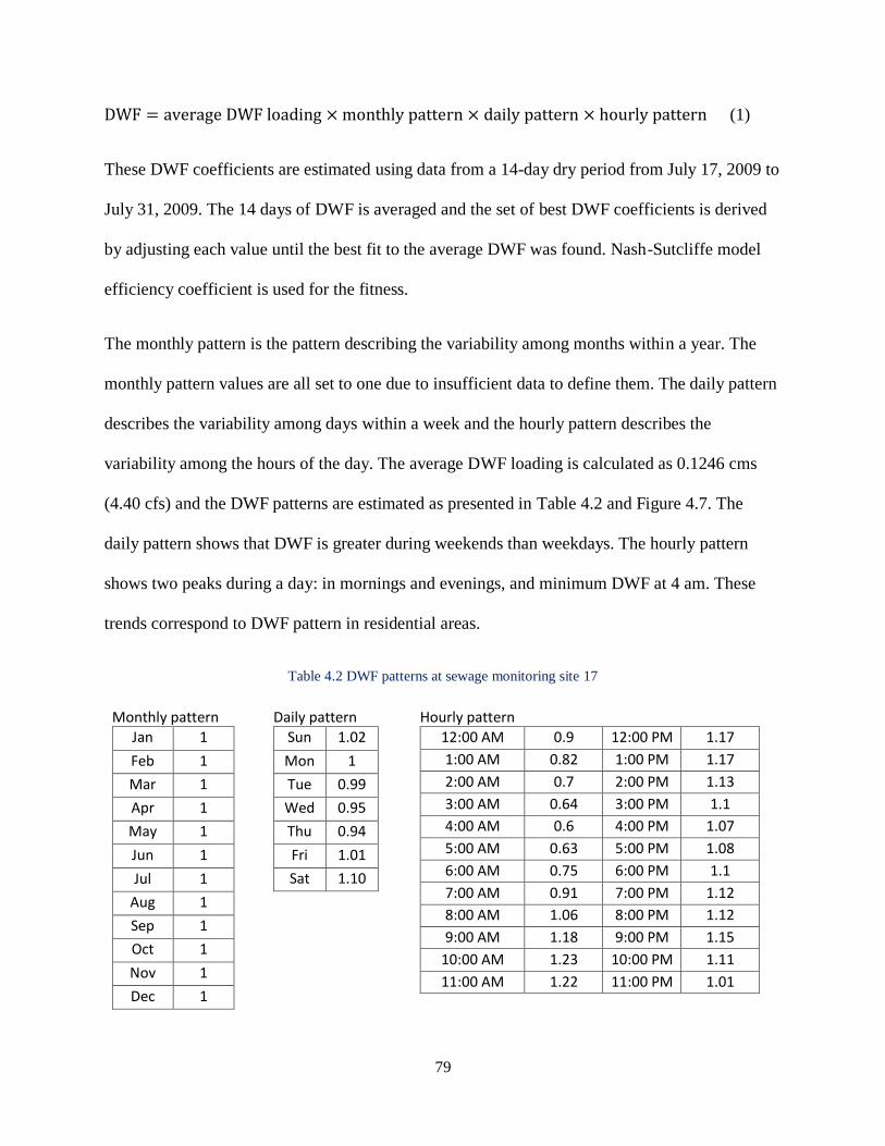
79

DWF = average DWF loading × monthly pattern × daily pattern × hourly pattern (1)

These DWF coefficients are estimated using data from a 14-day dry period from July 17, 2009 to

July 31, 2009. The 14 days of DWF is averaged and the set of best DWF coefficients is derived

by adjusting each value until the best fit to the average DWF was found. Nash-Sutcliffe model

efficiency coefficient is used for the fitness.

The monthly pattern is the pattern describing the variability among months within a year. The

monthly pattern values are all set to one due to insufficient data to define them. The daily pattern

describes the variability among days within a week and the hourly pattern describes the

variability among the hours of the day. The average DWF loading is calculated as 0.1246 cms

(4.40 cfs) and the DWF patterns are estimated as presented in Table 4.2 and Figure 4.7. The

daily pattern shows that DWF is greater during weekends than weekdays. The hourly pattern

shows two peaks during a day: in mornings and evenings, and minimum DWF at 4 am. These

trends correspond to DWF pattern in residential areas.

Table 4.2 DWF patterns at sewage monitoring site 17

Monthly pattern

Jan 1

Feb 1

Mar 1

Apr 1

May 1

Jun 1

Jul 1

Aug 1

Sep 1

Oct 1

Nov 1

Dec 1

Daily pattern

Sun 1.02

Mon 1

Tue 0.99

Wed 0.95

Thu 0.94

Fri 1.01

Sat 1.10

Hourly pattern

12:00 AM 0.9 12:00 PM 1.17

1:00 AM 0.82 1:00 PM 1.17

2:00 AM 0.7 2:00 PM 1.13

3:00 AM 0.64 3:00 PM 1.1

4:00 AM 0.6 4:00 PM 1.07

5:00 AM 0.63 5:00 PM 1.08

6:00 AM 0.75 6:00 PM 1.1

7:00 AM 0.91 7:00 PM 1.12

8:00 AM 1.06 8:00 PM 1.12

9:00 AM 1.18 9:00 PM 1.15

10:00 AM 1.23 10:00 PM 1.11

11:00 AM 1.22 11:00 PM 1.01

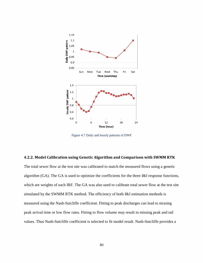
80

Figure 4.7 Daily and hourly patterns of DWF

4.2.2. Model Calibration using Genetic Algorithm and Comparison with SWMM RTK

The total sewer flow at the test site was calibrated to match the measured flows using a genetic

algorithm (GA). The GA is used to optimize the coefficients for the three I&I response functions,

which are weights of each IRF. The GA was also used to calibrate total sewer flow at the test site

simulated by the SWMM RTK method. The efficiency of both I&I estimation methods is

measured using the Nash-Sutcliffe coefficient. Fitting to peak discharges can lead to missing

peak arrival time or low flow rates. Fitting to flow volume may result in missing peak and tail

values. Thus Nash-Sutcliffe coefficient is selected to fit model result. Nash-Sutcliffe provides a

81

good fit for overall shape of sewer hydrograph as it is similar to root mean square. The equation

of the Nash-Sutcliffe model efficiency coefficient is defined as follows (Nash & Sutcliffe, 1970).

2

0

1

2

0 0

1

1

Tt t

m

t

Tt

t

Q Q

E

Q Q

(2)

where 0

tQ is observed discharge at time t, t

mQ is modeled discharge at time t, and 0Q is the

average of observed discharge. The coefficient ranges from -∞ to 1 and E = 1 corresponds to a

perfect match between the observed discharge and the modeled discharge.

As larger the Nash-Sutcliffe coefficient better the model fitting, maximizing the coefficient is set

as the objective function for the GA optimization. In actual formulation, the objective function is

to minimize 1- E. Initial guess of the weights of three IRFs are randomly selected.

Among the period of available data, the calibration period is selected from May 9, 2009 to June

7, 2009 and the validation period is from June 9, 2009 to July 8, 2009. The Impulse Response

Function (IRF) method has three parameters to calibrate: roof connection scaling factor (R),

sump pump connection scaling factor (S), and leaky lateral scaling factor (L). The three I&I

response function are derived using the physics-based models. The RTK method has nine

parameters to calibrate: R1, R2, R3, T1, T2, T3, K1, K2, and K3.

The GA optimization conditions for both IRF and RTK methods are presented as follows.

Size of the population = 100

Maximum number of generations = 300

82

The probability of crossover and the probability of mutation are also important GA settings. Box

plots in Figure 4.8 indicate how IRF parameters (a; roof connection coefficient, b; sump pump

connection coefficient, and c; leaky lateral coefficient) and Nash-Sutcliffe coefficients are

affected by the probability of crossover and the probability of mutation in the GA setting.

Different values of probability of crossover from 0.8 to 0.99 with 0.01 increments are tested in

Figure 4.8 (a). The probability of mutation is 0.06 for all cases. The solutions are unstable in the

range of crossover probability between 0.9 and 0.94 and more stable when it is greater than 0.95.

Thus 0.95 is selected as the probability of crossover for both IRF and RTK calibration. The

probability of mutation is tested from 0.01 to 0.2 as it appears in Figure 4.8 (b). The solutions

become unstable as the probability of mutation increases, especially when the probability is

greater than 0.11. Thus 0.06 is selected for both IRF and RTK calibration. The calibrated

parameter solutions for the IRF and RTK methods are presented in Table 4.4. The optimal

solution of the IRF method using the GA is: a = 3359 for roof, b = 22653 for sump pump, and c

= 19985 for lateral. These values can be interpreted as I&I volume contribution of each I&I

source. Contributing flow volume of each I&I source is derived by multiplying the per-unit-area

flow volume of IRFs and the IRF weighting coefficients. Then the contributing I&I volume from

the roof, sump pump, and lateral become 9710 m3, 22653 m3, and 32543 m3, respectively, and

they are 15%, 35%, and 50% of total estimated I&I flow volume. This simple calculation shows

that IRF result can be interpreted as I&I volume contribution of different I&I sources, which

shows the most problematic I&I contributor in the system volume-wise. The IRF model

application in this study is one realization of a real system and there is lots of uncertainty in the

system. However, this result still can provide insights to I&I behavior of the system by providing

physical meaning of the solutions.

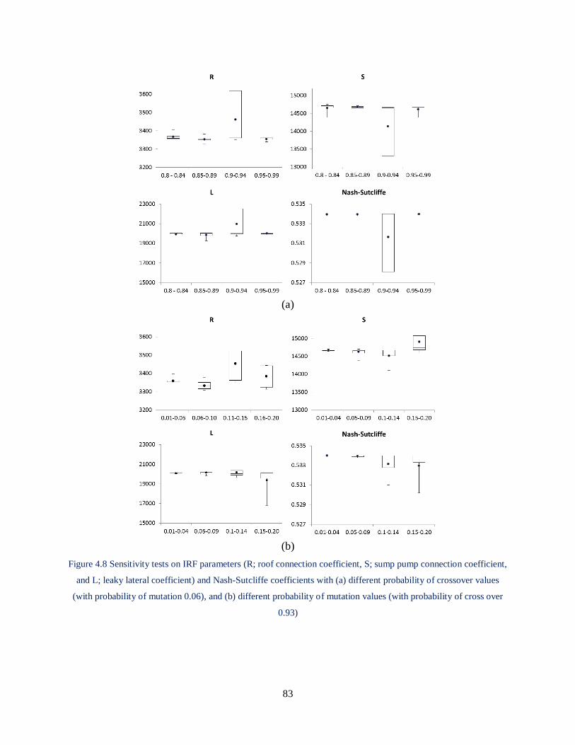
83

(a)

(b)

Figure 4.8 Sensitivity tests on IRF parameters (R; roof connection coefficient, S; sump pump connection coefficient,

and L; leaky lateral coefficient) and Nash-Sutcliffe coefficients with (a) different probability of crossover values

(with probability of mutation 0.06), and (b) different probability of mutation values (with probability of cross over

0.93)

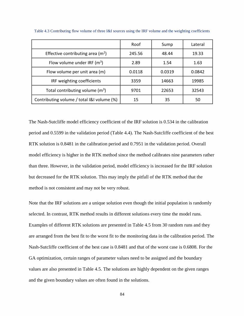
84

Table 4.3 Contributing flow volume of three I&I sources using the IRF volume and the weighting coefficients

Roof Sump Lateral

Effective contributing area (m2) 245.56 48.44 19.33

Flow volume under IRF (m3) 2.89 1.54 1.63

Flow volume per unit area (m) 0.0118 0.0319 0.0842

IRF weighting coefficients 3359 14663 19985

Total contributing volume (m3) 9701 22653 32543

Contributing volume / total I&I volume (%) 15 35 50

The Nash-Sutcliffe model efficiency coefficient of the IRF solution is 0.534 in the calibration

period and 0.5599 in the validation period (Table 4.4). The Nash-Sutcliffe coefficient of the best

RTK solution is 0.8481 in the calibration period and 0.7951 in the validation period. Overall

model efficiency is higher in the RTK method since the method calibrates nine parameters rather

than three. However, in the validation period, model efficiency is increased for the IRF solution

but decreased for the RTK solution. This may imply the pitfall of the RTK method that the

method is not consistent and may not be very robust.

Note that the IRF solutions are a unique solution even though the initial population is randomly

selected. In contrast, RTK method results in different solutions every time the model runs.

Examples of different RTK solutions are presented in Table 4.5 from 30 random runs and they

are arranged from the best fit to the worst fit to the monitoring data in the calibration period. The

Nash-Sutcliffe coefficient of the best case is 0.8481 and that of the worst case is 0.6808. For the

GA optimization, certain ranges of parameter values need to be assigned and the boundary

values are also presented in Table 4.5. The solutions are highly dependent on the given ranges

and the given boundary values are often found in the solutions.

85

RTK method has many local optimal solutions, which indicates that nine coefficients are not

independent. Thus the starting points or constraints of the parameters cause other parameters to

adjust to obtain a local optimum that behaves similarly for calibration data. Box plots of the nine

RTK parameters from the 30 model runs in Table 4.5 are presented in Figure 4.9 and three

triangular hydrographs from the parameters are shown in Figure 4.10. Greater variability is

observed in RTK parameters for the second and third triangular hydrographs, especially the third

one. This is because the model tries to adjust these parameters depending on the preceding

constraints.

Different RTK local solutions can result in the same model fitness. For example, case 15 and 16

in Table 4.5 show almost identical model fitness with Nash-Sutcliffe coefficients 0.7968 and

0.7937, respectively. However, T3 and K3 values are very different between those cases. Three

triangular hydrographs are constructed using the calibrated parameters for the two cases and

presented in Figure 4.11. Even with very similar R1 values (0.0242 and 0.0243), difference in T1

and K1 values result in a big difference in the peak of the first hydrograph with rhombus

markers. The peak of the first hydrograph in case 15 is 0.046 and that in case 16 is 0.091.

Duration of the third hydrographs with triangle markers are 27 hours and 209 hours for case 15

and 16, respectively. It is clearly shown that three hydrographs compensate each other and are

correlated. Change in one hydrograph affects other two hydrographs to simply achieve the best

fitness. Even with the difference between the triangular hydrographs, two cases simulated

monitoring data with very similar model fitness. This indicates the problem of the RTK method

that physical processes are not reflected in the modeling.

Because RTK method has nine parameters to adjust and they interact to each other, calibration

tends to be curve fitting rather than finding more physically based independent parameters. The

86

IRF approach tends to be more robust because three parameters adjust three IRF that represent

processes based on physics. Each IRF shape is defined independently using physics-based

models and the parameters weight the contribution from each of the three IRF. In contrast, the

RTK approach includes weighting parameters of each of the three hydrographs and two

parameters for each of the three hydrographs to adjust the shape of the hydrograph. Hence, the

calibration of the RTK method adjusts both the weights and the hydrograph shapes to obtain a

best fit to calibration data. Thus the RTK method is more likely to provide poor simulation of

response for conditions outside the calibration range.

Table 4.4 IRF-GA and RKT-GA results with Nash-Sutcliffe coefficients for the calibration period (May 9, 2009 to

June 7, 2009) and validation period (June 9, 2009 to July 8, 2009)

Method Estimated parameters Nash-Sutcliffe coefficient

Calibration Validation

IRF Roof connection scaling factor, a = 3359

Sump pump connection scaling factor, b = 14663 Leakey sewer lateral scaling factor, c = 19985

0.534 0.5599

RTK R1 = 0.02, T1 = 0.338, K1 = 2 R2 = 0.0478, T2 = 1, K2 = 10

R3 = 0.123, T3 = 8.5493, K3 = 14.6686 0.8481 0.7951

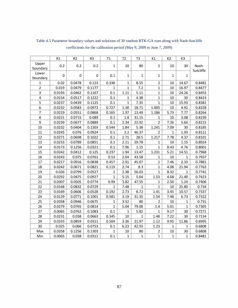
87

Table 4.5 Parameter boundary values and solutions of 30 random RTK-GA runs along with Nash-Sutcliffe

coefficients for the calibration period (May 9, 2009 to June 7, 2009)

R1 R2 R3 T1 T2 T3 K1 K2 K3

Nash- Sutcliffe

Upper boundary

0.2 0.2 0.2 1 10 80 2 10 30

Lower boundary

0 0 0 0.1 1 1 1 1 1

1 0.02 0.0478 0.123 0.338 1 8.55 2 10 14.67 0.8481

2 0.019 0.0479 0.1177 1 1 7.2 1 10 16.97 0.8477

3 0.0193 0.0462 0.1167 0.1 1.11 5.11 1 10 24.26 0.8453

4 0.0154 0.0517 0.1222 0.1 1 4.38 1 10 30 0.8424

5 0.0237 0.0439 0.1125 0.1 1 7.35 1 10 15.93 0.8381

6 0.0232 0.0583 0.0972 0.727 1.38 18.71 1.005 10 4.92 0.8328

7 0.0219 0.0551 0.0868 0.165 1.97 13.49 1.186 5.73 7.77 0.8264

8 0.0221 0.0715 0.089 0.1 1.8 31.15 1 10 3.08 0.8239

9 0.0239 0.0677 0.0889 0.1 2.34 22.92 2 7.26 5.66 0.8215

10 0.0232 0.0404 0.1303 0.544 1.84 5.38 1.241 7.09 30 0.8185

11 0.0245 0.076 0.0924 0.1 2.2 46.37 2 1 1.93 0.8111

12 0.0271 0.0698 0.1022 0.1 2.71 28.5 1.217 7.78 4.37 0.8101

13 0.0233 0.0789 0.0851 0.1 2.11 59.78 1 10 1.15 0.8024

14 0.0173 0.1256 0.0321 0.1 7.96 1.15 1 8.43 4.76 0.8001

15 0.0242 0.0412 0.125 0.237 1.94 13.47 1.231 5.21 14.51 0.7968

16 0.0243 0.075 0.0761 0.53 2.04 43.58 1 10 1 0.7937

17 0.0217 0.0916 0.0838 0.457 2.91 45.07 1 7.46 2.33 0.7881

18 0.0242 0.0671 0.0821 0.119 2.74 8.3 1 4.08 21.94 0.7763

19 0.026 0.0799 0.0527 1 2.38 56.03 1 8.32 1 0.7741

20 0.0292 0.0475 0.0927 1 5.15 5.64 1.53 4.68 21.40 0.7423

21 0.0307 0.0505 0.0774 0.99 3.82 47.55 1 2.50 1.24 0.7406

22 0.0168 0.0832 0.0729 1 7.48 1 1 10 25.80 0.734

23 0.0169 0.0606 0.0528 0.192 2.73 8.72 1.41 3.45 10.57 0.7337

24 0.0129 0.0771 0.1001 0.581 3.19 31.35 1.54 7.48 6.73 0.7322

25 0.0358 0.0946 0.0675 1 3.52 80 2 10 1 0.731

26 0.0279 0.0765 0.0814 1 5.04 79.08 1.4 5.01 1 0.7305

27 0.0065 0.0762 0.1083 0.1 1 5.82 1 9.17 30 0.7271

28 0.0231 0.038 0.0663 0.345 10 1 1.48 7.22 30 0.7134

29 0.0333 0.0859 0.0311 0.504 3.36 21.97 1.12 9.95 11.86 0.6995

30 0.025 0.066 0.0753 0.1 6.23 42.93 1.23 1 1 0.6808

Max 0.0358 0.1256 0.1303 1 10 80 2 10 30 0.6808

Min 0.0065 0.038 0.0311 0.1 1 1 1 1 1 0.8481

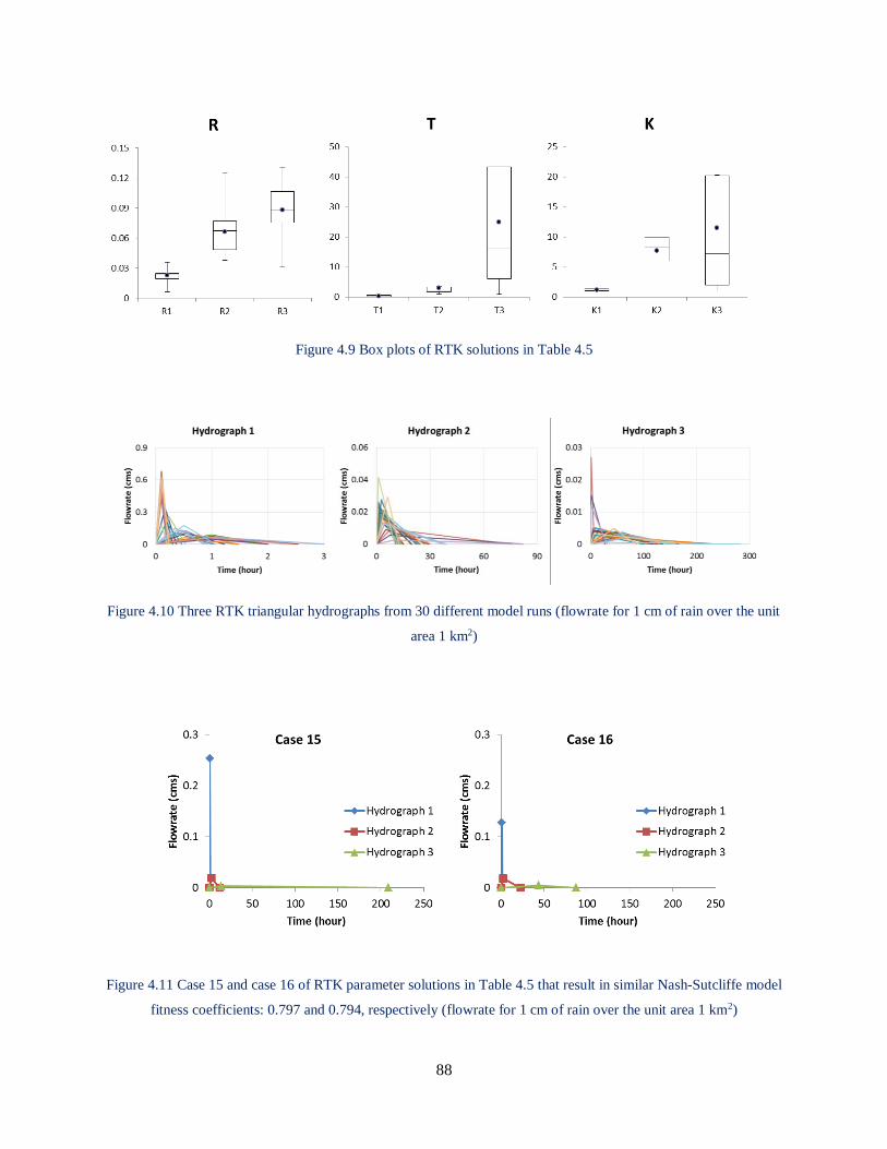
88

Figure 4.9 Box plots of RTK solutions in Table 4.5

Figure 4.10 Three RTK triangular hydrographs from 30 different model runs (flowrate for 1 cm of rain over the unit

area 1 km2)

Figure 4.11 Case 15 and case 16 of RTK parameter solutions in Table 4.5 that result in similar Nash-Sutcliffe model

fitness coefficients: 0.797 and 0.794, respectively (flowrate for 1 cm of rain over the unit area 1 km2)

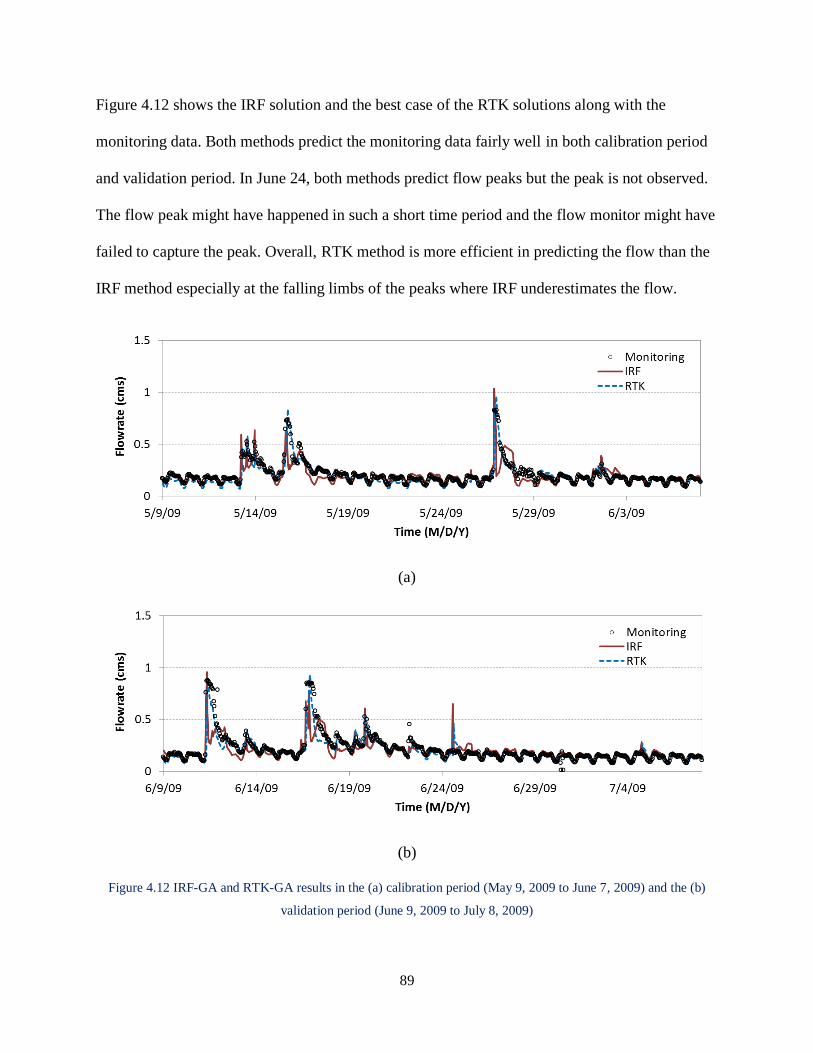
89

Figure 4.12 shows the IRF solution and the best case of the RTK solutions along with the

monitoring data. Both methods predict the monitoring data fairly well in both calibration period

and validation period. In June 24, both methods predict flow peaks but the peak is not observed.

The flow peak might have happened in such a short time period and the flow monitor might have

failed to capture the peak. Overall, RTK method is more efficient in predicting the flow than the

IRF method especially at the falling limbs of the peaks where IRF underestimates the flow.

(a)

(b)

Figure 4.12 IRF-GA and RTK-GA results in the (a) calibration period (May 9, 2009 to June 7, 2009) and the (b)

validation period (June 9, 2009 to July 8, 2009)

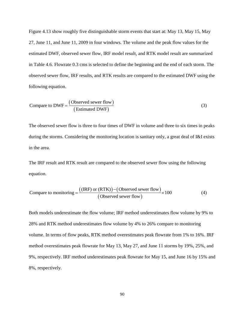
90

Figure 4.13 show roughly five distinguishable storm events that start at: May 13, May 15, May

27, June 11, and June 11, 2009 in four windows. The volume and the peak flow values for the

estimated DWF, observed sewer flow, IRF model result, and RTK model result are summarized

in Table 4.6. Flowrate 0.3 cms is selected to define the beginning and the end of each storm. The

observed sewer flow, IRF results, and RTK results are compared to the estimated DWF using the

following equation.

Observed sewer flowCompare to DWF

Estimated DWF (3)

The observed sewer flow is three to four times of DWF in volume and three to six times in peaks

during the storms. Considering the monitoring location is sanitary only, a great deal of I&I exists

in the area.

The IRF result and RTK result are compared to the observed sewer flow using the following

equation.

(IRF) or (RTK) Observed sewer flowCompare to monitoring 100

Observed sewer flow

(4)

Both models underestimate the flow volume; IRF method underestimates flow volume by 9% to

28% and RTK method underestimates flow volume by 4% to 26% compare to monitoring

volume. In terms of flow peaks, RTK method overestimates peak flowrate from 1% to 16%. IRF

method overestimates peak flowrate for May 13, May 27, and June 11 storms by 19%, 25%, and

9%, respectively. IRF method underestimates peak flowrate for May 15, and June 16 by 15% and

8%, respectively.

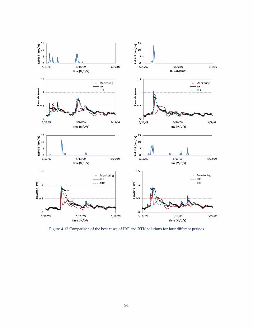
91

Figure 4.13 Comparison of the best cases of IRF and RTK solutions for four different periods

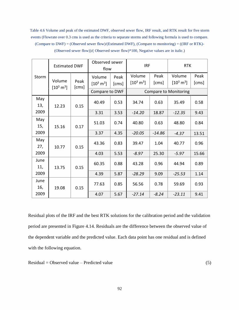
92

Table 4.6 Volume and peak of the estimated DWF, observed sewer flow, IRF result, and RTK result for five storm

events (Flowrate over 0.3 cms is used as the criteria to separate storms and following formula is used to compare.

(Compare to DWF) = (Observed sewer flow)/(Estimated DWF), (Compare to monitoring) = ((IRF or RTK)-

(Observed sewer flow))/( Observed sewer flow)*100, Negative values are in italic.)

Storm

Estimated DWF Observed sewer

flow IRF RTK

Volume

[103 m3]

Peak [cms]

Volume

[103 m3]

Peak

[cms]

Volume

[103 m3]

Peak

[cms]

Volume

[103 m3]

Peak

[cms]

Compare to DWF Compare to Monitoring

May

13,

2009 12.23 0.15

40.49 0.53 34.74 0.63 35.49 0.58

3.31 3.53 -14.20 18.87 -12.35 9.43

May

15,

2009

15.16 0.17 51.03 0.74 40.80 0.63 48.80 0.84

3.37 4.35 -20.05 -14.86 -4.37 13.51

May

27,

2009

10.77 0.15 43.36 0.83 39.47 1.04 40.77 0.96

4.03 5.53 -8.97 25.30 -5.97 15.66

June

11,

2009

13.75 0.15 60.35 0.88 43.28 0.96 44.94 0.89

4.39 5.87 -28.29 9.09 -25.53 1.14

June

16,

2009

19.08 0.15 77.63 0.85 56.56 0.78 59.69 0.93

4.07 5.67 -27.14 -8.24 -23.11 9.41

Residual plots of the IRF and the best RTK solutions for the calibration period and the validation

period are presented in Figure 4.14. Residuals are the difference between the observed value of

the dependent variable and the predicted value. Each data point has one residual and is defined

with the following equation.

Residual = Observed value – Predicted value (5)

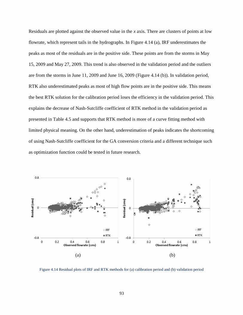
93

Residuals are plotted against the observed value in the x axis. There are clusters of points at low

flowrate, which represent tails in the hydrographs. In Figure 4.14 (a), IRF underestimates the

peaks as most of the residuals are in the positive side. These points are from the storms in May

15, 2009 and May 27, 2009. This trend is also observed in the validation period and the outliers

are from the storms in June 11, 2009 and June 16, 2009 (Figure 4.14 (b)). In validation period,

RTK also underestimated peaks as most of high flow points are in the positive side. This means

the best RTK solution for the calibration period loses the efficiency in the validation period. This

explains the decrease of Nash-Sutcliffe coefficient of RTK method in the validation period as

presented in Table 4.5 and supports that RTK method is more of a curve fitting method with

limited physical meaning. On the other hand, underestimation of peaks indicates the shortcoming

of using Nash-Sutcliffe coefficient for the GA conversion criteria and a different technique such

as optimization function could be tested in future research.

(a) (b)

Figure 4.14 Residual plots of IRF and RTK methods for (a) calibration period and (b) validation period

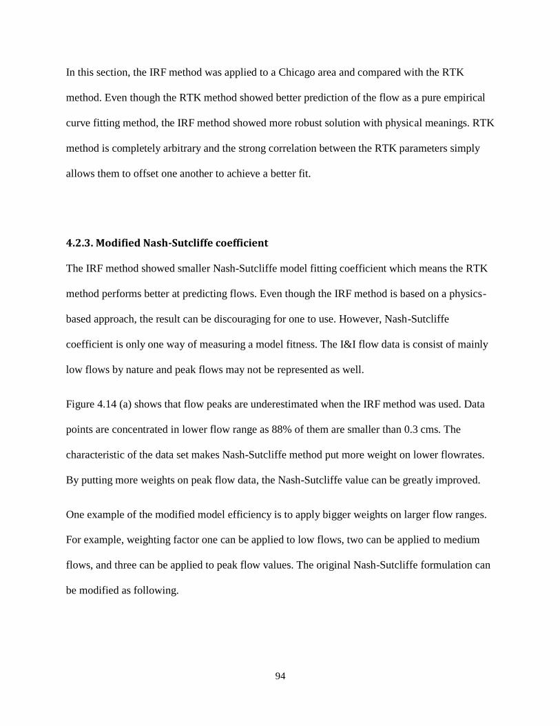
94

In this section, the IRF method was applied to a Chicago area and compared with the RTK

method. Even though the RTK method showed better prediction of the flow as a pure empirical

curve fitting method, the IRF method showed more robust solution with physical meanings. RTK

method is completely arbitrary and the strong correlation between the RTK parameters simply

allows them to offset one another to achieve a better fit.

4.2.3. Modified Nash-Sutcliffe coefficient

The IRF method showed smaller Nash-Sutcliffe model fitting coefficient which means the RTK

method performs better at predicting flows. Even though the IRF method is based on a physics-

based approach, the result can be discouraging for one to use. However, Nash-Sutcliffe

coefficient is only one way of measuring a model fitness. The I&I flow data is consist of mainly

low flows by nature and peak flows may not be represented as well.

Figure 4.14 (a) shows that flow peaks are underestimated when the IRF method was used. Data

points are concentrated in lower flow range as 88% of them are smaller than 0.3 cms. The

characteristic of the data set makes Nash-Sutcliffe method put more weight on lower flowrates.

By putting more weights on peak flow data, the Nash-Sutcliffe value can be greatly improved.

One example of the modified model efficiency is to apply bigger weights on larger flow ranges.

For example, weighting factor one can be applied to low flows, two can be applied to medium

flows, and three can be applied to peak flow values. The original Nash-Sutcliffe formulation can

be modified as following.

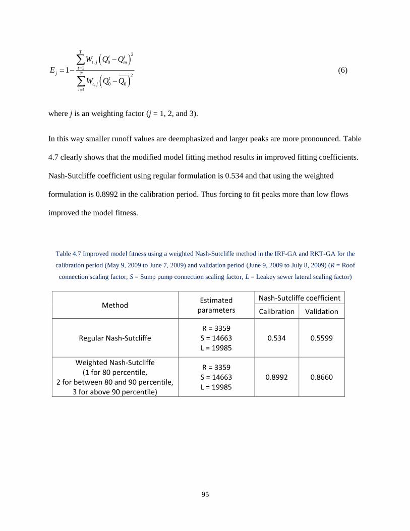
95

2

, 0

1

2

, 0 0

1

1

Tt t

t j m

tj T

t

t j

t

W Q Q

E

W Q Q

(6)

where j is an weighting factor (j = 1, 2, and 3).

In this way smaller runoff values are deemphasized and larger peaks are more pronounced. Table

4.7 clearly shows that the modified model fitting method results in improved fitting coefficients.

Nash-Sutcliffe coefficient using regular formulation is 0.534 and that using the weighted

formulation is 0.8992 in the calibration period. Thus forcing to fit peaks more than low flows

improved the model fitness.

Table 4.7 Improved model fitness using a weighted Nash-Sutcliffe method in the IRF-GA and RKT-GA for the

calibration period (May 9, 2009 to June 7, 2009) and validation period (June 9, 2009 to July 8, 2009) (R = Roof

connection scaling factor, S = Sump pump connection scaling factor, L = Leakey sewer lateral scaling factor)

Method Estimated

parameters

Nash-Sutcliffe coefficient

Calibration Validation

Regular Nash-Sutcliffe

R = 3359

S = 14663

L = 19985

0.534 0.5599

Weighted Nash-Sutcliffe

(1 for 80 percentile, 2 for between 80 and 90 percentile,

3 for above 90 percentile)

R = 3359

S = 14663

L = 19985 0.8992 0.8660

96

References

Espey Jr., W. H., Clemmens, B., & Halverson, B. (2014) Lake Michigan Diversion Committee:

Findings of the seventh technical committee for review of diversion flow measurements and

accounting procedures (p. 124). Chicago, IL.

Hickory Hills (zip 60457), Illinois Climate. (2014, June). Retrieved January 6, 2016, from

http://www.bestplaces.net/climate/zip-code/illinois/hickory_hills/60457.

Miller, K., & Schmidt, A. R. (2010) Hydraulic modeling of the Calumet interceptor network,

Tunnel and Reservoir plan, Report No.10. Urbana, IL.

Nash, J. E., & Sutcliffe, J. V. (1970) River flow forecasting through conceptual models, Part I - a

discussion of principles. Journal of Hydrology, 10, 282–290.

U.S. Census Bureau, Profile of General Population and Housing characteristics: 2010

Demographic Profile Data (DP-1): Hickory Hills city, Illinois, American Factfinder.

Retrieved January 6, 2016 from

http://factfinder.census.gov/faces/tableservices/jsf/pages/productview.xhtml?src=bkmk.

97

5. Uncertainty in Rainfall Induced Infiltration

5.1. Introduction

This study suggests a lumped model of I&I using scaling factors of three I&I hydrographs that

are derived from physics-based models. Thus error is expected to be introduced in the modeling.

In this chapter, possible uncertainties in rainfall induced infiltration (RII) through a leaky pipe

are examined. Uncertainty resulting from the following six factors is independently examined:

antecedent moisture condition (AMC), pedotransfer functions (PTFs), soil hydraulic

conductivities, sewer pipe depths, initial conditions (IC), and rainfall characteristics.

Uncertainty in unsaturated flow modeling can be divided into two kinds: intrinsic uncertainty

and information uncertainty (Dettinger & Wilson 1981). Tung & Yen (2005) referred to these

two kinds of uncertainty as natural variability and knowledge deficiency (Figure 1). The six

factors under the uncertainty investigation involve uncertainties from both natural variability and

knowledge deficiency. In Table1, uncertainty sources related to the six factors of interest are

summarized. Since the impact of all the uncertainty sources is either difficult or impractical to

measure, the uncertainty investigation is performed only for limited sources as described in the

following paragraphs.

Antecedent moisture condition (AMC) includes the uncertainty related to climatic, hydrologic,

and geologic natural variability as well as data deficiency. In this study, the effect of variable

AMC between storms on infiltration hydrograph is investigated thus the interest is only focused

on short term climatic variability.

98

Pedotransfer functions (PTFs) are closely connected with the uncertainty in soil hydraulic

conductivity. PTFs are empirical models that are developed to reduce the uncertainty in

estimating hydraulic conductivity by using directly measurable soil properties (e.g. soil

composition). However, directly measurable soil properties also involve uncertainties: geologic

variability and knowledge deficiency in data. There are various PTFs to choose from and

different PTFs give different solutions, which also results in model uncertainty. More easily

measurable soil property values are also limited. Thus the error is from natural variability,

insufficient data, and different PTF models. In this study, seven different PTFs are tested using

the same soil properties in the test area and the hydraulic conductivity values that are derived

from the PTFs are compared to each other.

The soil hydraulic conductivity is used as a model parameter in this study and the uncertainty is

originated from geologic variability (e.g. non-uniform ground condition), knowledge deficiency

in model parameter and data (e.g. limited data availability), and measurement error. The impact

of different hydraulic conductivity values on the infiltration hydrograph is examined.

Sewer pipe depths affect the infiltration hydrograph and involve uncertainty mainly from

knowledge deficiency, data measurement errors, inadequate sampling, and error caused by

handling and transcription mistakes. The effect of different sewer pipe depths on the RII

hydrograph is investigated.

The infiltration model has a start-up period where the solution has not converged to equilibrium.

The duration required for the start-up period depends on the initial condition (IC). However, the

solution eventually converges to a stable behavior no matter what the ICs are. This implies that

this is a boundary-value problem. The infiltration model does not converge until the effect of the

99

boundary condition dissipates. Ten different simulation periods are tested to investigate the

effect of IC on the infiltration hydrograph and to estimate the average start-up period.

Different rainfall characteristics affect the infiltration response and both natural variability,

especially climatic variability, and data deficiency cause the uncertainty. To understand the

impact of rainfall characteristics on the RII hydrograph, various storm durations and shapes are

applied in the modeling.

This study suggests a lumped I&I model using representative IRFs that are applied across

sewershed with scaling parameters. The lumped model introduces error but it is impossible to

physically model every flow path into the sewer system. For example, depths of all sewer pipes

in the sewershed are different. Hydraulic conductivity values vary from lateral locations and

depth. Thus this chapter is prepared to investigate uncertainty introduced by the variability of the

modeling factors. Each factor is examined independently and changes in IRF to uniform rainfall

or unsaturated flow response to actual rainfall are evaluated by changing model inputs.

To see how AMC affects IRF, IRFs for a uniform rainfall following different AMCs is

evaluated. For comparison of different PTFs, seven different PTFs are simply applied to the

same soil data to determine the estimated hydraulic conductivity resulting from different PTF.

For hydraulic conductivity, unsaturated flow response to the real rainfall is compared with

different hydraulic conductivity values that cover the range of measured hydraulic conductivity

and calculated ones from the PTFs. Different sewer depths are tested for the infiltration model

with real rainfall and the unsaturated flow responses are compared. The infiltration model start-

up periods vary for different simulation periods. Thus the start-up periods for nine different

simulation periods, and the average start-up period are calculated. For rainfall characteristics,

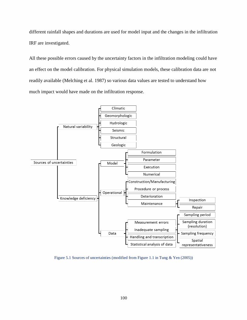
100

different rainfall shapes and durations are used for model input and the changes in the infiltration

IRF are investigated.

All these possible errors caused by the uncertainty factors in the infiltration modeling could have

an effect on the model calibration. For physical simulation models, these calibration data are not

readily available (Melching et al. 1987) so various data values are tested to understand how

much impact would have made on the infiltration response.

Figure 5.1 Sources of uncertainties (modified from Figure 1.1 in Tung & Yen (2005))

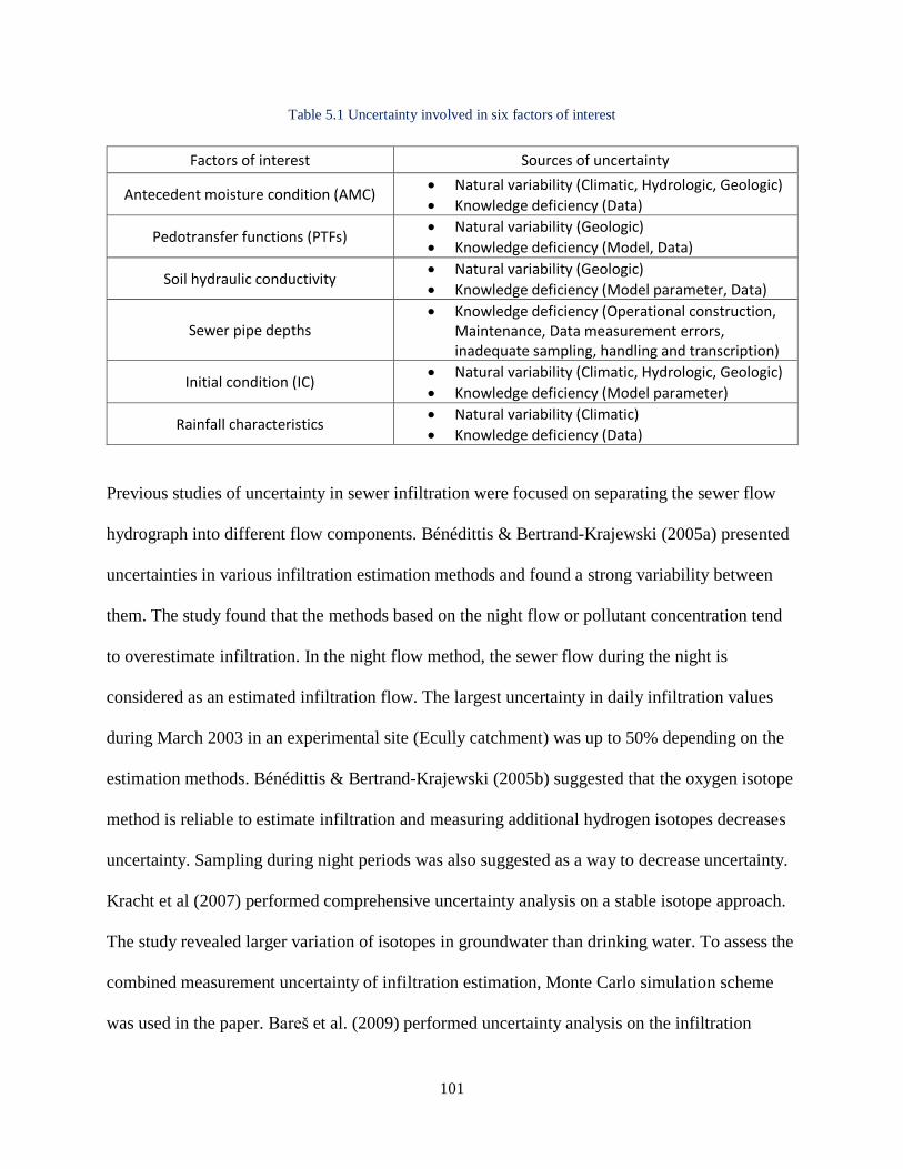
101

Table 5.1 Uncertainty involved in six factors of interest

Factors of interest Sources of uncertainty

Antecedent moisture condition (AMC) Natural variability (Climatic, Hydrologic, Geologic)

Knowledge deficiency (Data)

Pedotransfer functions (PTFs) Natural variability (Geologic)

Knowledge deficiency (Model, Data)

Soil hydraulic conductivity Natural variability (Geologic)

Knowledge deficiency (Model parameter, Data)

Sewer pipe depths Knowledge deficiency (Operational construction,

Maintenance, Data measurement errors, inadequate sampling, handling and transcription)

Initial condition (IC) Natural variability (Climatic, Hydrologic, Geologic)

Knowledge deficiency (Model parameter)

Rainfall characteristics Natural variability (Climatic)

Knowledge deficiency (Data)

Previous studies of uncertainty in sewer infiltration were focused on separating the sewer flow

hydrograph into different flow components. Bénédittis & Bertrand-Krajewski (2005a) presented

uncertainties in various infiltration estimation methods and found a strong variability between

them. The study found that the methods based on the night flow or pollutant concentration tend

to overestimate infiltration. In the night flow method, the sewer flow during the night is

considered as an estimated infiltration flow. The largest uncertainty in daily infiltration values

during March 2003 in an experimental site (Ecully catchment) was up to 50% depending on the

estimation methods. Bénédittis & Bertrand-Krajewski (2005b) suggested that the oxygen isotope

method is reliable to estimate infiltration and measuring additional hydrogen isotopes decreases

uncertainty. Sampling during night periods was also suggested as a way to decrease uncertainty.

Kracht et al (2007) performed comprehensive uncertainty analysis on a stable isotope approach.

The study revealed larger variation of isotopes in groundwater than drinking water. To assess the

combined measurement uncertainty of infiltration estimation, Monte Carlo simulation scheme

was used in the paper. Bareš et al. (2009) performed uncertainty analysis on the infiltration

102

estimation using pollutant load and continuous water quality and quantity monitoring. The

analysis found that chemical oxygen demand (COD) is preferred as a natural tracer over total

suspended solid (TSS). Starting time during a day and sampling interval also affected

uncertainty; larger uncertainty was observed for longer sampling interval. Franz (2007) applied

modified multivariate statistical technique to optimize sewer measuring points and the new

method reduced up to 40% of uncertainty related to measurements. These study efforts only have

provided insights on uncertainty in measurements of flows or substances in wastewater. These

studies also focused on groundwater infiltration to sewer systems rather than RII.

Pawlowski et al. (2013) found that storm intensity and AMC affects the contribution of different

I&I sources to the total rainfall derived infiltration and inflow volume. Contribution of I&I from

downspout connections increased with high intensity storms under dry AMC and the flow

contribution from faulty sewer lateral increased with low intensity storms under wet AMC. By

investigating the impact of the six variables in RII, this study will provide better understanding

about sewer infiltration modeling.

5.2. Uncertainty Factors

5.2.1. Antecedent Moisture Condition

The effect of AMC on RII is evaluated by adding a perturbation into the rainfall record and

comparing with the control case, which is the result without the perturbation. The perturbation is

the uniform 3-hour, 42-mm rainfall presented in section 4.1.2 and this is added at ten different

random times in the rainfall record. The list of random times is presented in Table 1 of chapter 4

and the changed hyetographs are presented in Figure 5.2. The IRFs of the perturbation are

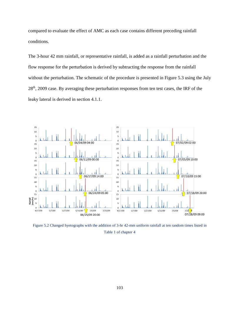
103

compared to evaluate the effect of AMC as each case contains different preceding rainfall

conditions.

The 3-hour 42 mm rainfall, or representative rainfall, is added as a rainfall perturbation and the

flow response for the perturbation is derived by subtracting the response from the rainfall

without the perturbation. The schematic of the procedure is presented in Figure 5.3 using the July

28th, 2009 case. By averaging these perturbation responses from ten test cases, the IRF of the

leaky lateral is derived in section 4.1.1.

Figure 5.2 Changed hyetographs with the addition of 3-hr 42-mm uniform rainfall at ten random times listed in

Table 1 of chapter 4

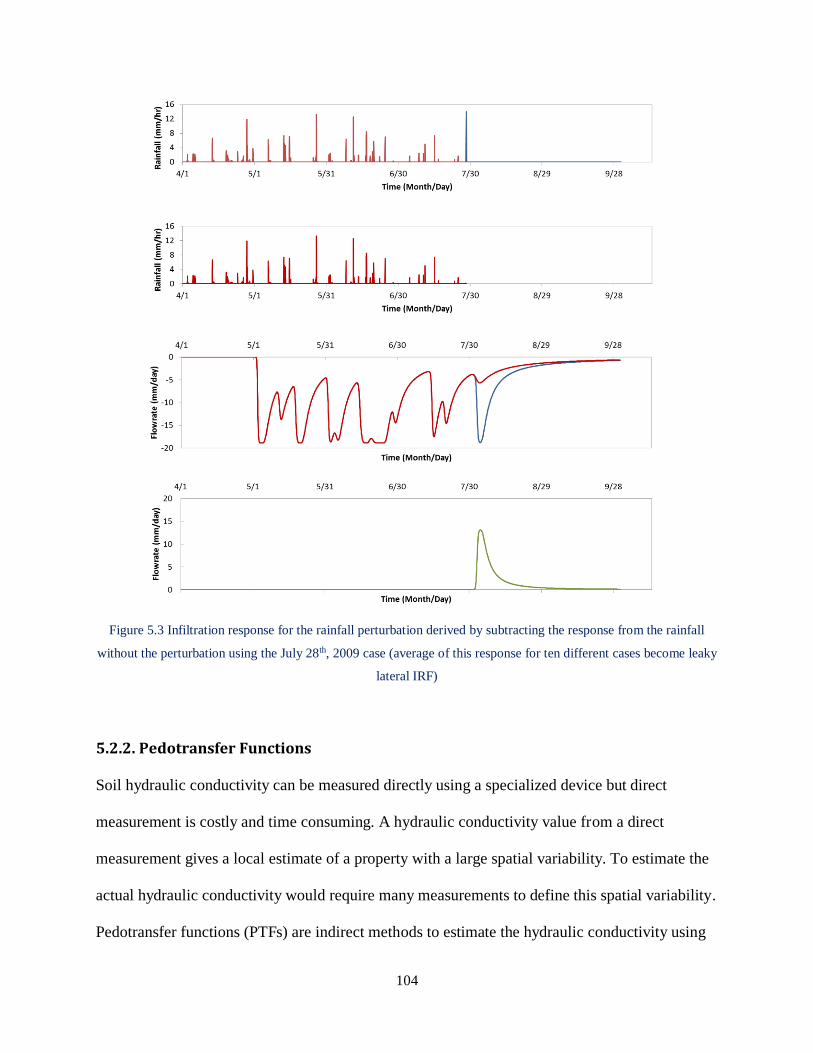
104

Figure 5.3 Infiltration response for the rainfall perturbation derived by subtracting the response from the rainfall

without the perturbation using the July 28th, 2009 case (average of this response for ten different cases become leaky

lateral IRF)

5.2.2. Pedotransfer Functions

Soil hydraulic conductivity can be measured directly using a specialized device but direct

measurement is costly and time consuming. A hydraulic conductivity value from a direct

measurement gives a local estimate of a property with a large spatial variability. To estimate the

actual hydraulic conductivity would require many measurements to define this spatial variability.

Pedotransfer functions (PTFs) are indirect methods to estimate the hydraulic conductivity using

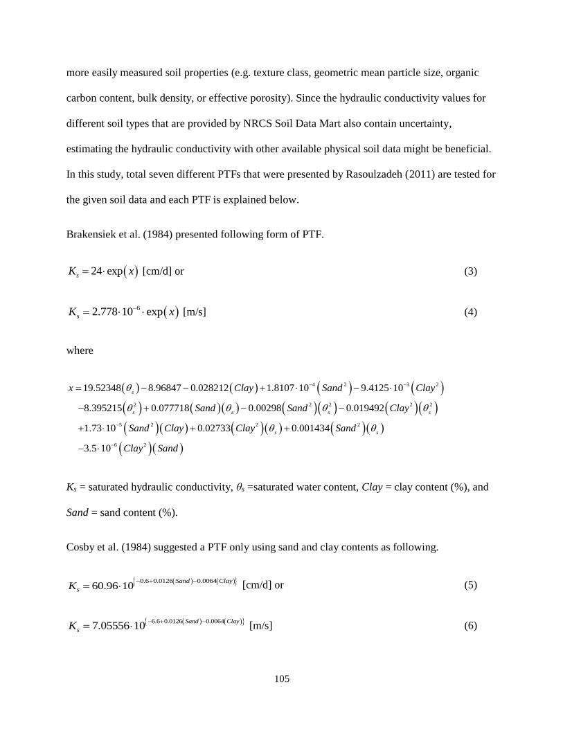
105

more easily measured soil properties (e.g. texture class, geometric mean particle size, organic

carbon content, bulk density, or effective porosity). Since the hydraulic conductivity values for

different soil types that are provided by NRCS Soil Data Mart also contain uncertainty,

estimating the hydraulic conductivity with other available physical soil data might be beneficial.

In this study, total seven different PTFs that were presented by Rasoulzadeh (2011) are tested for

the given soil data and each PTF is explained below.

Brakensiek et al. (1984) presented following form of PTF.

24 expsK x [cm/d] or (3)

62.778 10 expsK x [m/s] (4)

where

4 2 3 2

2 2 2 2 2

5 2 2 2

6 2

19.52348 8.96847 0.028212 1.8107 10 9.4125 10

8.395215 0.077718 0.00298 0.019492

1.73 10 0.02733 0.001434

3.5 10

s

s s s s

s s

x Clay Sand Clay

Sand Sand Clay

Sand Clay Clay Sand

Clay Sand

Ks = saturated hydraulic conductivity, θs =saturated water content, Clay = clay content (%), and

Sand = sand content (%).

Cosby et al. (1984) suggested a PTF only using sand and clay contents as following.

0.6 0.0126 0.006460.96 10

Sand Clay

sK

[cm/d] or (5)

6.6 0.0126 0.00647.05556 10

Sand Clay

sK

[m/s] (6)

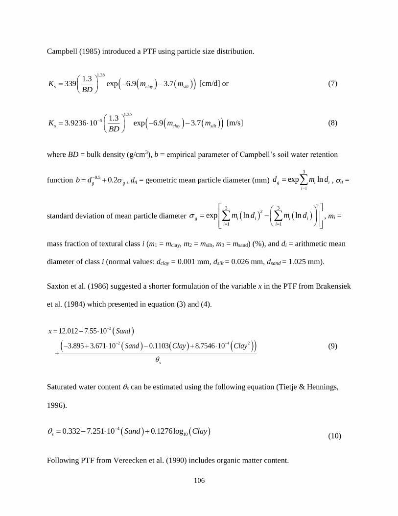
106

Campbell (1985) introduced a PTF using particle size distribution.

1.3

1.3339 exp 6.9 3.7

b

s clay siltK m mBD

[cm/d] or (7)

1.3

5 1.33.9236 10 exp 6.9 3.7

b

s clay siltK m mBD

[m/s] (8)

where BD = bulk density (g/cm3), b = empirical parameter of Campbell’s soil water retention

function 0.5 0.2g gb d , dg = geometric mean particle diameter (mm)

3

1

exp lng i i

i

d m d

, g =

standard deviation of mean particle diameter 2

3 32

1 1

exp ln lng i i i i

i i

m d m d

, mi =

mass fraction of textural class i (m1 = mclay, m2 = msilt, m3 = msand) (%), and di = arithmetic mean

diameter of class i (normal values: dclay = 0.001 mm, dsilt = 0.026 mm, dsand = 1.025 mm).

Saxton et al. (1986) suggested a shorter formulation of the variable x in the PTF from Brakensiek

et al. (1984) which presented in equation (3) and (4).

2

2 4 2

12.012 7.55 10

3.895 3.671 10 0.1103 8.7546 10

s

x Sand

Sand Clay Clay

(9)

Saturated water content s can be estimated using the following equation (Tietje & Hennings,

1996).

4

100.332 7.251 10 0.1276logs Sand Clay (10)

Following PTF from Vereecken et al. (1990) includes organic matter content.

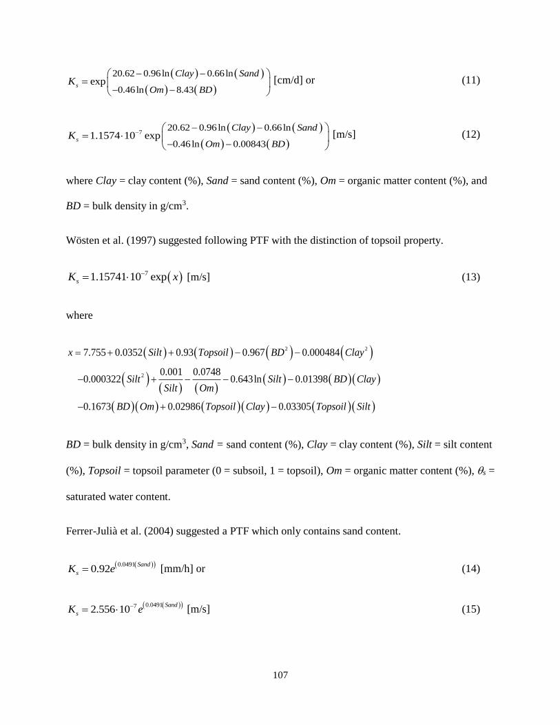
107

20.62 0.96ln 0.66ln

0.46ln 8.43exps

Clay Sand

Om BDK

[cm/d] or (11)

7

20.62 0.96ln 0.66ln

0.46ln 0.008431.1574 10 exps

Clay Sand

Om BDK

[m/s] (12)

where Clay = clay content (%), Sand = sand content (%), Om = organic matter content (%), and

BD = bulk density in g/cm3.

Wösten et al. (1997) suggested following PTF with the distinction of topsoil property.

71.15741 10 expsK x [m/s] (13)

where

2 2

2

7.755 0.0352 0.93 0.967 0.000484

0.001 0.07480.000322 0.643ln 0.01398

0.1673 0.02986 0.03305

x Silt Topsoil BD Clay

Silt Silt BD ClaySilt Om

BD Om Topsoil Clay Topsoil Silt

BD = bulk density in g/cm3, Sand = sand content (%), Clay = clay content (%), Silt = silt content

(%), Topsoil = topsoil parameter (0 = subsoil, 1 = topsoil), Om = organic matter content (%), s =

saturated water content.

Ferrer-Julià et al. (2004) suggested a PTF which only contains sand content.

0.04910.92

Sand

sK e [mm/h] or (14)

0.049172.556 10Sand

sK e [m/s] (15)

108

5.2.3. Soil Hydraulic Conductivities

Hydraulic conductivity is often considered as one of the most difficult factors to estimate in

unsaturated flow modeling (El-Kadi 1987, Baroni et al. 2010). Three different soil properties are

used to represent ambient soil, impermeable soil, and extremely permeable soil in the model. The

impermeable soil represents impervious surface areas (e.g. sidewalks, and buildings). The

extremely permeable soil characterizes the leaky sewer pipe. The hydraulic conductivity for both

soil layers are assumed as 10-12 m/s and 10-2 m/s, respectively. Various hydraulic conductivity

values for the ambient soil are presented in Table 5.2 for testing. The actual soil data are

obtained from NRCS Soil Data Mart for a sample area, Hickory Hills, IL, and the testing values

in Table 5.2 are determined based on the data distribution. The area-weighted average value of

hydraulic conductivity in the area is 2.1910-7 m/s and 16 cases with different hydraulic

conductivity values are tested. Note that case 15 and 16 are based on the hydraulic conductivity

Table 5.2 Hydraulic conductivity values for the test

Cumulative area % smaller Ks (m/s)

1 5 4.6110-8

2 10 5.0710-8

3 20 5.9810-8

4 25 (30) 6.5310-8

5 40 6.7010-8

6 50 7.1710-8

7 60 7.6010-8

8 70 1.0610-7

9 Area weighted average 2.1910-7

10 75 3.1410-7

11 80 6.1910-7

12 85 6.3210-7

13 90 6.4410-7

14 95 6.5710-7

15 Additional case (1st quartile of PTF results) 1.2810-6

16 Additional case (3rd quartile of PTF results) 1.8010-6

109

values derived from the application result of different PTFs that is presented in the later section

5.3.2 in this chapter.

5.2.4. Sewer Pipe Depths

The sewer pipe depth determines the length of unsaturated flow paths. To estimate the sewer

depth in the study area, the digitized sewer map for Hickory Hills, IL is analyzed. Figure 5.4 is

the illustration of sewer junctions in the area and available data points are highlighted. The total

number of junctions in the area is 1089 and 713 have both invert and ground elevations

available, which is 65% of the entire junctions.

Figure 5.4 Sewer junctions in Hickory Hills, IL with elevation data availability

A junction depth is defined as the difference between the ground elevation and the junction

invert elevation. The frequency plot of the junction depths is presented in Figure 5.5.The average

sewer depth is 2.62 m, median depth is 2.42 m, and the most frequent depth is 2.44 m. Thus the

sewer lateral depth for the representative case is assumed as 2.5 m for convenience. To evaluate

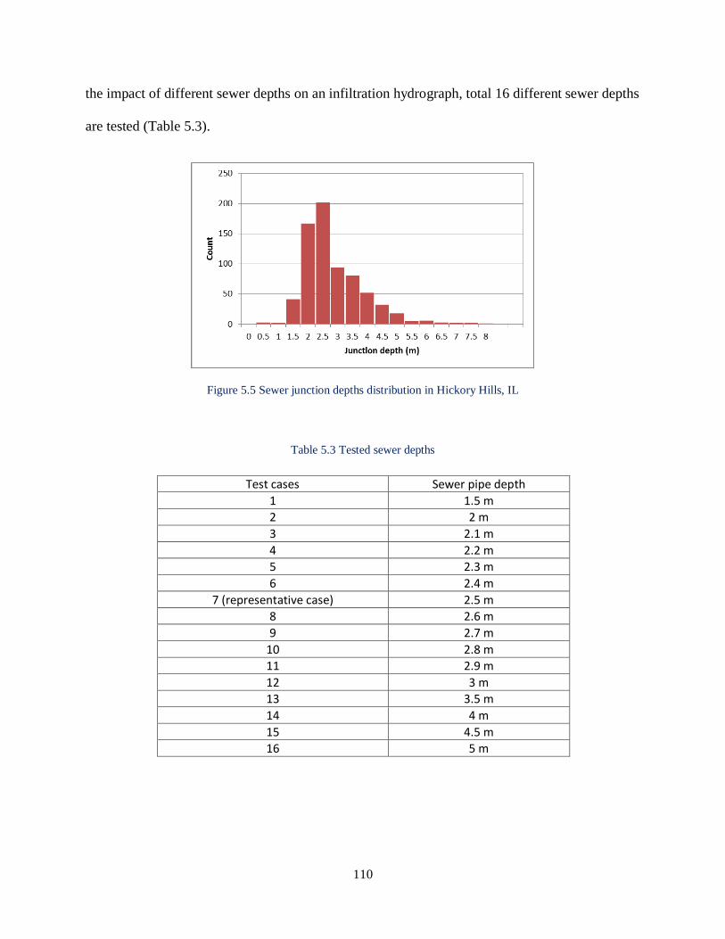
110

the impact of different sewer depths on an infiltration hydrograph, total 16 different sewer depths

are tested (Table 5.3).

Figure 5.5 Sewer junction depths distribution in Hickory Hills, IL

Table 5.3 Tested sewer depths

Test cases Sewer pipe depth

1 1.5 m

2 2 m

3 2.1 m

4 2.2 m

5 2.3 m

6 2.4 m

7 (representative case) 2.5 m

8 2.6 m

9 2.7 m

10 2.8 m

11 2.9 m

12 3 m

13 3.5 m

14 4 m

15 4.5 m

16 5 m

111

5.2.5. Initial Condition

To investigate the effect of IC on the RII hydrograph and to determine the average model start-

up period, nine different simulation periods are randomly selected as test cases (Table 5.4). RII

responses from the nine test cases are compared with the response from the control case, which

includes the whole simulation period from January 1, 2009 to July 30, 2009. Test cases are

selected within the control period with different starting time and the control case starts early

enough that the boundary value effect is dissipated by the time the flow response is compared to

the test cases.

Table 5.4 Test cases with different simulation start times to investigate the initial condition (IC)

Test cases Sewer pipe depth

1 1.5 m

2 2 m

3 2.1 m

4 2.2 m

5 2.3 m

6 2.4 m

7 (representative case) 2.5 m

8 2.6 m

9 2.7 m

10 2.8 m

5.2.6. Rainfall Characteristics

To investigate the impact of different rainfall durations and rainfall shapes, total nine various

rainfall cases are tested (Figure 5.6). The test cases are variations of the control rainfall, which is

the uniform rainfall with 3 hour duration and 42 mm volume. Five different rainfall durations: 1-

hour, 6-hours, 12-hour, 24-hour, and 48-hours, and three different triangular hyetographs:

forward skewed, centered, and backward skewed, are tested with the same rainfall volume.

These perturbations are arbitrarily included in real rainfall record and the RII hydrographs are

compared after subtracting the original hydrograph without the perturbations (Figure 5.7).

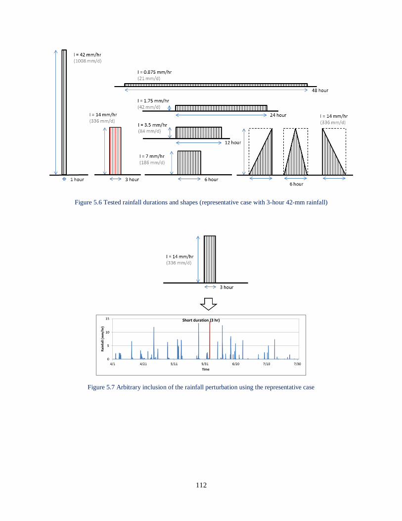
112

Figure 5.6 Tested rainfall durations and shapes (representative case with 3-hour 42-mm rainfall)

Figure 5.7 Arbitrary inclusion of the rainfall perturbation using the representative case

113

5.3. Results and Discussion

5.3.1. Antecedent Moisture Condition

The RII flow responses at the leaky sewer lateral with the uniform rainfall at different times are

presented in Figure 5.8. The overall average infiltration response of all the cases is presented

with black solid lines throughout the plots. Figure 5.8 (a), (b), and (c) show three distinguishable

infiltration flow response shapes. The three shapes are named forward, centered, and backward

responses based on the way that the peaks are skewed. Figure 5.8 (a) illustrates the forward

infiltration responses with the average forward response shown with a dashed line. The forward

response shows higher peak that precedes the peak of the overall average response (shown by the

solid line). Figure 5.8 (b) shows the centered infiltration responses with the average shown by

dashed line. This matches well with the overall average response. Figure 5.8 (c) illustrates the

backward infiltration responses with the average backward response shown by a dashed line. The

backward response also has a higher peak that follows the peak of the overall average in time. In

Figure 5.8 (d), the cumulative depths of rainfall in the N days preceding the storm events being

examined are shown, with the number of days, N, given on the x-axis. The three curves shown

illustrate the cumulative rainfall preceding the event for average forward, centered, and

backward events. Difference in cumulative rainfall depths for the three cases is clear until 29

days. Forward response is the result of drier antecedent conditions and backward response is due

to wetter antecedent condition. Centered response falls in between them. A rainfall event in drier

periods (cumulative rainfall for 29 days ≈ 20 mm) brings the forward response in the infiltration.

Rainfall in wetter periods (cumulative rainfall for 29 days ≈ 60 mm) results in backward

response. The ones in between (20 mm < cumulative rainfall for 29 days < 60 mm) cause

centered response, which matches with the overall average infiltration response. In terms of the

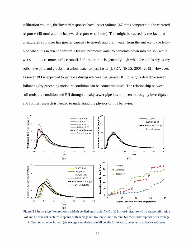
114

infiltration volume, the forward responses have larger volume (47 mm) compared to the centered

response (45 mm) and the backward responses (44 mm). This might be caused by the fact that

unsaturated soil layer has greater capacity to absorb and drain water from the surface to the leaky

pipe when it is in drier condition. Dry soil promotes water to percolate down into the soil while

wet soil induces more surface runoff. Infiltration rate is generally high when the soil is dry as dry

soils have pore and cracks that allow water to pass faster (USDA-NRCS, 2001, 2012). However,

as sewer I&I is expected to increase during wet weather, greater RII through a defective sewer

following dry preceding moisture condition can be counterintuitive. The relationship between

soil moisture condition and RII through a leaky sewer pipe has not been thoroughly investigated

and further research is needed to understand the physics of this behavior.

(a) (b)

(c) (d)

Figure 5.8 Infiltration flow response with three distinguishable AMCs (a) forward response with average infiltration

volume 47 mm, (b) centered response with average infiltration volume 45 mm, (c) backward response with average

infiltration volume 44 mm, (d) average cumulative rainfall depths for forward, centered, and backward cases

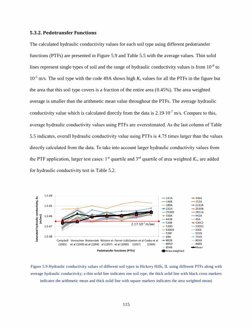
115

5.3.2. Pedotransfer Functions

The calculated hydraulic conductivity values for each soil type using different pedotransfer

functions (PTFs) are presented in Figure 5.9 and Table 5.5 with the average values. Thin solid

lines represent single types of soil and the range of hydraulic conductivity values is from 10-8 to

10-5 m/s. The soil type with the code 49A shows high Ks values for all the PTFs in the figure but

the area that this soil type covers is a fraction of the entire area (0.45%). The area weighted

average is smaller than the arithmetic mean value throughout the PTFs. The average hydraulic

conductivity value which is calculated directly from the data is 2.1910-7 m/s. Compare to this,

average hydraulic conductivity values using PTFs are overestimated. As the last column of Table

5.5 indicates, overall hydraulic conductivity value using PTFs is 4.75 times larger than the values

directly calculated from the data. To take into account larger hydraulic conductivity values from

the PTF application, larger test cases: 1st quartile and 3rd quartile of area weighted Ks, are added

for hydraulic conductivity test in Table 5.2.

Figure 5.9 Hydraulic conductivity values of different soil types in Hickory Hills, IL using different PTFs along with

average hydraulic conductivity; a thin solid line indicates one soil type, the thick solid line with black cross markers

indicates the arithmetic mean and thick solid line with square markers indicates the area weighted mean)

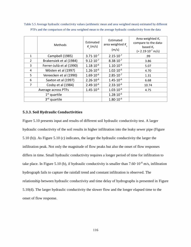
116

Table 5.5 Average hydraulic conductivity values (arithmetic mean and area weighted mean) estimated by different

PTFs and the comparison of the area weighted mean to the average hydraulic conductivity from the data

Methods Estimated

Ks (m/s)

Estimated area weighted K

s

(m/s)

Area weighted Ks compare to the data-

based Ks

(= 2.1910-7 m/s)

1 Campbell (1985) 3.7110-7 2.1510-7 .99

2 Brakensiek et al (1984) 9.1210-7 8.3810-7 3.86

3 Ferrer-Julià et al (1990) 1.1810-6 1.1010-6 5.07

4 Wösten et al (1997) 1.2610-6 1.0210-6 4.70

5 Vereecken et al (1990) 1.6910-6 2.8510-7 1.31

6 Saxton et al (1997) 2.2610-6 1.4510-6 6.68

7 Cosby et al (1984) 2.4910-6 2.3310-6 10.74

Average across PTFs 1.4510-6 1.0310-6 4.75

1st quartile 1.2810-6

3rd quartile 1.8010-6

5.3.3. Soil Hydraulic Conductivities

Figure 5.10 presents input and results of different soil hydraulic conductivity test. A larger

hydraulic conductivity of the soil results in higher infiltration into the leaky sewer pipe (Figure

5.10 (b)). As Figure 5.10 (c) indicates, the larger the hydraulic conductivity the larger the

infiltration peak. Not only the magnitude of flow peaks but also the onset of flow responses

differs in time. Small hydraulic conductivity requires a longer period of time for infiltration to

take place. In Figure 5.10 (b), if hydraulic conductivity is smaller than 7.60·10-8 m/s, infiltration

hydrograph fails to capture the rainfall trend and constant infiltration is observed. The

relationship between hydraulic conductivity and time delay of hydrographs is presented in Figure

5.10(d). The larger hydraulic conductivity the slower flow and the longer elapsed time to the

onset of flow response.

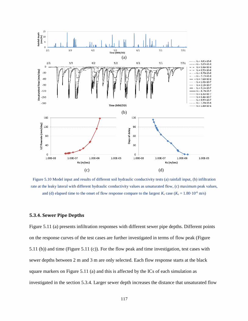
117

(a)

(b)

(c) (d)

Figure 5.10 Model input and results of different soil hydraulic conductivity tests (a) rainfall input, (b) infiltration

rate at the leaky lateral with different hydraulic conductivity values as unsaturated flow, (c) maximum peak values,

and (d) elapsed time to the onset of flow response compare to the largest Ks case (Ks = 1.80·10-6 m/s)

5.3.4. Sewer Pipe Depths

Figure 5.11 (a) presents infiltration responses with different sewer pipe depths. Different points

on the response curves of the test cases are further investigated in terms of flow peak (Figure

5.11 (b)) and time (Figure 5.11 (c)). For the flow peak and time investigation, test cases with

sewer depths between 2 m and 3 m are only selected. Each flow response starts at the black

square markers on Figure 5.11 (a) and this is affected by the ICs of each simulation as

investigated in the section 5.3.4. Larger sewer depth increases the distance that unsaturated flow

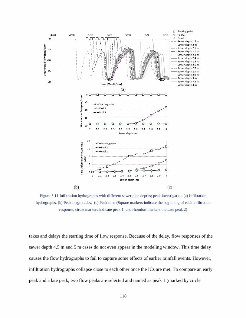
118

(a)

(b) (c)

Figure 5.11 Infiltration hydrographs with different sewer pipe depths; peak investigation (a) Infiltration

hydrographs, (b) Peak magnitudes, (c) Peak time (Square markers indicate the beginning of each infiltration

response, circle markers indicate peak 1, and rhombus markers indicate peak 2)

takes and delays the starting time of flow response. Because of the delay, flow responses of the

sewer depth 4.5 m and 5 m cases do not even appear in the modeling window. This time delay

causes the flow hydrographs to fail to capture some effects of earlier rainfall events. However,

infiltration hydrographs collapse close to each other once the ICs are met. To compare an early

peak and a late peak, two flow peaks are selected and named as peak 1 (marked by circle

119

markers) and peak 2 (marked by rhombus markers) in Figure 5.11. Peak 1 is still under the effect

of IC so the magnitude and time change greatly depending on the sewer depths. Compare to peak

1, a little difference is found in peak 2 in terms of the peak magnitude and the time. This is

because the solution comes to the equilibrium with time. Thus different sewer depths does not

affect peak flow rate greatly once the effect of IC dissipates.

Not only peak values in the infiltration curves but also tail values in the receding limbs are

investigated in Figure 5.12. The term “tail” is used for the lowest points of receding limbs here.

To compare an early tail and a late tail, two flow tails are selected and named tail 1 (marked by

circle markers) and tail 2 (marked by rhombus markers) in Figure 5.12. As Figure 5.12 (b) and

Figure 5.12 (c) indicate, the infiltration hydrographs shift consistently at tail points as the slope

of the graphs appear constant. In Figure 5.12 (b), the slope of the tail 1 curve is 1.2710-3 /day

and that of the tail 2 curve is 1.2410-3 /day. This means that one meter of sewer depth change

causes changes in infiltration rate by 1.2710-3 mm/day and 1.2410-3 mm/day in tail values for

the first and the second receding limbs respectively. A larger sewer pipe depth results in longer

time of a tail to reach the pipe. The slope of time curves in Figure 5.12 (c) is 2.67 day/m and 2.83

day/m for tail 1 and tail 2 groups respectively. This implies that one meter change in sewer depth

causes average 2.67 day and 2.84 day of time delay of the tail points in the first and the second

receding limbs respectively. These values have to be perceived with a caution since they may

change depending on interevent time of rainfall data and soil hydraulic conductivity values.

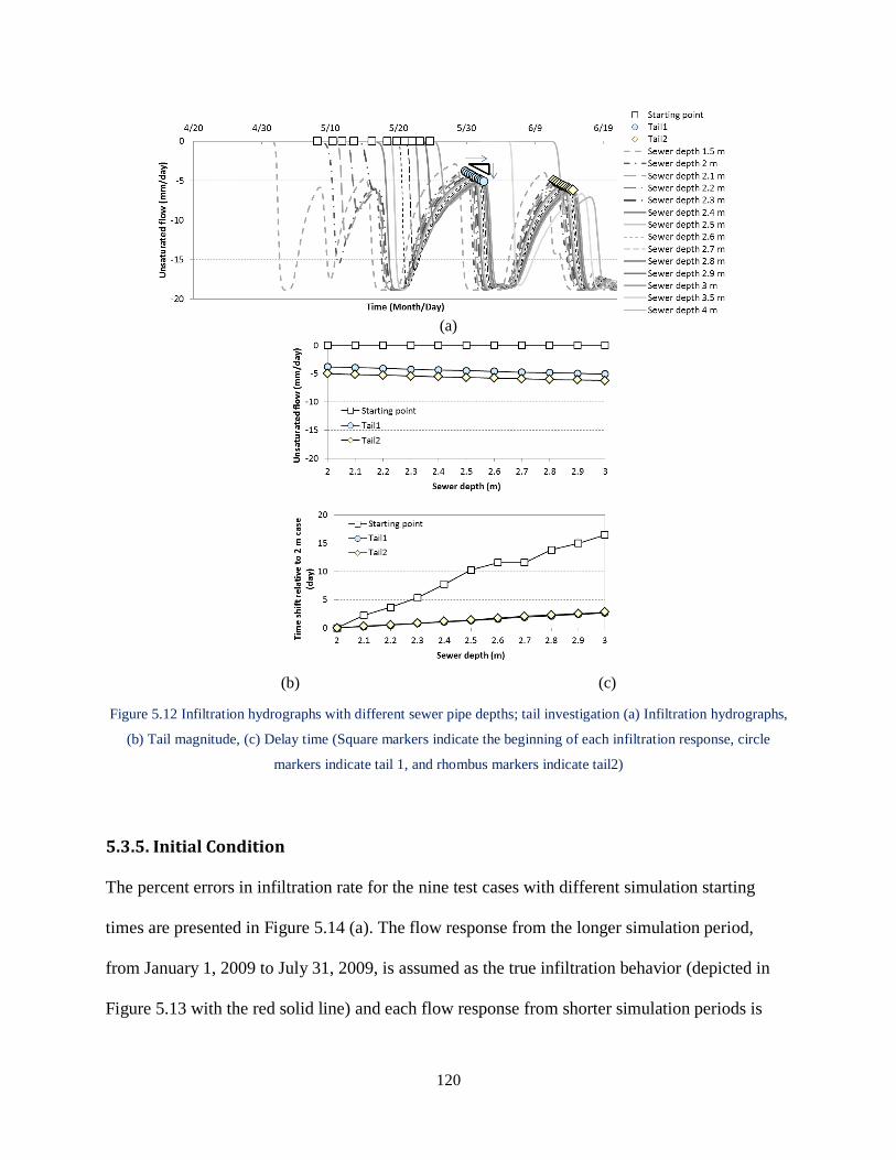
120

(a)

(b) (c)

Figure 5.12 Infiltration hydrographs with different sewer pipe depths; tail investigation (a) Infiltration hydrographs,

(b) Tail magnitude, (c) Delay time (Square markers indicate the beginning of each infiltration response, circle

markers indicate tail 1, and rhombus markers indicate tail2)

5.3.5. Initial Condition

The percent errors in infiltration rate for the nine test cases with different simulation starting

times are presented in Figure 5.14 (a). The flow response from the longer simulation period,

from January 1, 2009 to July 31, 2009, is assumed as the true infiltration behavior (depicted in

Figure 5.13 with the red solid line) and each flow response from shorter simulation periods is

121

compared to this true value to calculate the error. An example of the test case that converges on

Marcy 3, 2009 is illustrated in Figure 5.13 with the blue solid line. The definition of percent error

is presented as

ErrorPercent error 100

True or theoretical value (18)

where Error is the difference between experimental value and true value (Error = Experimental

value – True or theoretical value).

Most of the error curves show sudden change from -100% to near 0% at different times. This

transition from -100% to 0% is observed no later than 20 days of simulation for all the cases. The

median and average errors are presented in Figure 5.14 (b) along with the maximum, minimum,

1st quartile, and 3rd quartile values. Difference between the median and average curves in the

figure indicates a skewed distribution of the data. Overall the average percent error decreases

with time and most of the error is dissipated after 20 days. This result is when the sewer pipe

depth is 2.5 m and different sewer depth will result in change of the length of the warm-up

period.

Figure 5.13 Comparison of infiltration response for the converged case and the test case of March 3rd, 2009

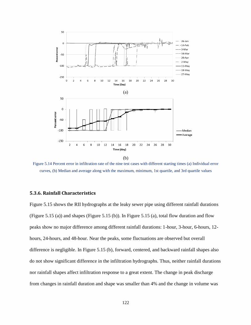
122

(a)

(b)

Figure 5.14 Percent error in infiltration rate of the nine test cases with different starting times (a) Individual error

curves, (b) Median and average along with the maximum, minimum, 1st quartile, and 3rd quartile values

5.3.6. Rainfall Characteristics

Figure 5.15 shows the RII hydrographs at the leaky sewer pipe using different rainfall durations

(Figure 5.15 (a)) and shapes (Figure 5.15 (b)). In Figure 5.15 (a), total flow duration and flow

peaks show no major difference among different rainfall durations: 1-hour, 3-hour, 6-hours, 12-

hours, 24-hours, and 48-hour. Near the peaks, some fluctuations are observed but overall

difference is negligible. In Figure 5.15 (b), forward, centered, and backward rainfall shapes also

do not show significant difference in the infiltration hydrographs. Thus, neither rainfall durations

nor rainfall shapes affect infiltration response to a great extent. The change in peak discharge

from changes in rainfall duration and shape was smaller than 4% and the change in volume was

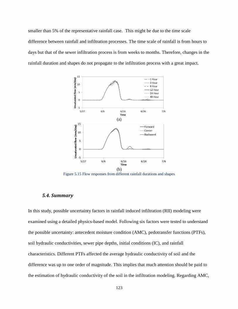
123

smaller than 5% of the representative rainfall case. This might be due to the time scale

difference between rainfall and infiltration processes. The time scale of rainfall is from hours to

days but that of the sewer infiltration process is from weeks to months. Therefore, changes in the

rainfall duration and shapes do not propagate to the infiltration process with a great impact.

(a)

(b)

Figure 5.15 Flow responses from different rainfall durations and shapes

5.4. Summary

In this study, possible uncertainty factors in rainfall induced infiltration (RII) modeling were

examined using a detailed physics-based model. Following six factors were tested to understand

the possible uncertainty: antecedent moisture condition (AMC), pedotransfer functions (PTFs),

soil hydraulic conductivities, sewer pipe depths, initial conditions (IC), and rainfall

characteristics. Different PTFs affected the average hydraulic conductivity of soil and the

difference was up to one order of magnitude. This implies that much attention should be paid to

the estimation of hydraulic conductivity of the soil in the infiltration modeling. Regarding AMC,

124

an infiltration peak arrived earlier in a hydrograph and total infiltration volume increased during

dry periods. In contrast, the onset of the peak occurred later and the total infiltration volume

decreased during wet periods. The overall results showed that the most sensitive factor among

them was the soil hydraulic conductivity and this soil property defined the maximum infiltration

rate. Different sewer depths brought different model start-up periods. A larger sewer depth

required longer start-up period since it increased the distance of flow paths. In terms of IC,

roughly 20 days of start-up period were required to guarantee the error gets dissipated and the

flow response finally reflects the rainfall effect. Different rainfall durations and shapes did not

affect the infiltration hydrographs as much as other factors. This is because the time scale of

rainfall is much shorter than the infiltration process. These findings bring insights to the sewer

infiltration modeling and better understanding of the uncertainty underlies the sewer infiltration

process.

125

References

Bareš, V., Stránský, D., & Sýkora, P. (2009) Sewer infiltration/inflow: long-term monitoring

based on diurnal variation of pollutant mass flux. Water Science and Technology : A

Journal of the International Association on Water Pollution Research, 60(1), 1–7.

doi:10.2166/wst.2009.280

Baroni, G., Facchi, A., Gandolfi, C., Ortuani, B., Horeschi, D., & Dam, J. C. van. (2010)

Uncertainty in the determination of soil hydraulic parameters and its influence on the

performance of two hydrological models of different complexity. Hydrology and Earth

System Science, 14, 251–270.

Brakensiek, D. L., Rawls, W. J., & Stephenson, G. R. (1984) Modifying SCS hydrologic soil

groups and curve numbers for rangeland soils. ASAE Paper No. PNR-84-203. St. Joseph,

MI.

Campbell, G. S. (1985) Soil Physics With Basic: Transport Models for Soil-Plant Systems (p.

149). New York: Elsevier.

Cosby, B. J., Hornberger, G. M., Clapp, R. B., & Ginn, T. R. (1984) A Statistical Exploration of

the Relationships of Soil Moisture Characteristics to the Physical Properties of Soils. Water

Resources Research, 20(6), 682. doi:10.1029/WR020i006p00682

De Bénédittis, J., & Bertrand-Krajewski, J. L. (2005a) Infiltration in sewer systems: comparison

of measurement methods. Water Science and Technology : A Journal of the International

126

Association on Water Pollution Research, 52(3), 219–27. Retrieved from


De Bénédittis, J., & Bertrand-Krajewski, J. L. (2005b) Measurement of infiltration rates in urban

sewer systems by use of oxygen isotopes. Water Science and Technology: A Journal of the

International Association on Water Pollution Research, 52(3), 229–37. Retrieved from


Dettinger, M. D., & Wilson, J. L. (1981) First order analysis of uncertainty in numerical models

of groundwater flow Part 1. Mathematical development. Water Resources Research, 17(1),

149–161.

DHI Software. (2007a) MIKE SHE user manual volume 1: user guide, Vol. 1.

DHI Software. (2007b) MIKE SHE user manual volume 2: reference guide, Vol. 2.

El-Kadi, A. I. (1987) Variability of infiltration under uncertainty in unsaturated zone parameters.

Journal of Hydrology, 90(1-2), 61–80. doi:10.1016/0022-1694(87)90173-9

Ferrer-Julià, M., Estrela Monreal, T., Sánchez del Corral Jiménez, A., & Garcı́a Meléndez, E.

(2004) Constructing a saturated hydraulic conductivity map of Spain using pedotransfer

functions and spatial prediction. Geoderma, 123(3-4), 257–277.

doi:10.1016/j.geoderma.2004.02.011



127

Kracht, O., Gresch, M., & Gujer, W. (2007) A stable isotope approach for the quantification of

sewer infiltration. Environmental Science and Technology technology, 41(16), 5839–45.

Retrieved from http://www.ncbi.nlm.nih.gov/pubmed/17874795

Melching, C. S., Yen, B. C., & Wenzel Jr., H. G. (1987) WRC Research Report No. 208,

Incorporation of uncertainties in real-time catchment flood forecasting (p. 194). Urbana,

IL.

USDA-NRCS. (2001) Soil quality information sheet: Rangeland soil quality — Infiltration.

USDA-NRCS. (2012) Soil infiltration: Soil quality kit - Guides for educators.

NRCS Soil Data Mart http://soildatamart.nrcs.usda.gov/

Pawlowski, C. W., Rhea, L., Shuster, W. D., & Barden, G. (2013) Some factors affecting inflow

and infiltration from residential sources in a core urban area: A case study in a Columbus

OH USA neighborhood. Journal of Hydraulic Engineering. doi:10.1061/(ASCE)HY.1943-

7900.0000799

Rasoulzadeh, A. (2011) Estimating hydraulic conductivity using pedotransfer functions. In L.

Elango (Ed.), Hydraulic Conductivity - Issues, Determination and Applications (pp. 145–

164). InTech.

Saxton, K.E., Rawls, W.J., Romberger, J.S., and Papendick, R.I. (1986) Estimating generalized

soil water characteristics from texture. Soil Science Society of America Journal 50: 1301-

1036.

128

Tietje, O. & Hennings, V. (1996) Accuracy of the saturated hydraulic conductivity prediction by

pedo-transfer functions compared to the variability within FAO textural classes. Geoderma

69(1-2), 71–84. doi:10.1016/0016-7061(95)00050-X

Tung, Y., & Yen, B. (2005) Uncertainties in hydrosystems engineering and management. In

Hydrosystems engineering uncertainty analysis (pp. 1–12). McGraw-Hill.

Vereecken, H., Maes, J., and Feyen, J. (1990) Estimating unsaturated hydraulic conductivity

from easily measured soil properties. Soil Science 149: 1-12.

Wösten, J.H.M. (1997) Pedotransfer functions to evaluate soil quality. In:Gegorich, E.G., Carter,

M.R. (Eds.), Soil Quality for Crop Production and Ecosystem Health. Developments in

Soils Science, vol. 25, Elsesevier, Amesterdam 221-245.

Wösten, J.H.M., Lilly, A., Nemes, A., and Le Bas, C. (1999) Development and use of a database

of hydraulic properties of European soils. Geoderma 90: 169-185.

129

Summary and Conclusions

This study was conducted to investigate detailed I&I physical processes for three major sources

of I&I into urban sewer systems: roof downspout, sump pump, and leaky lateral. The I&I

response for the representative uniform rainfall from each of the three sources is referred to as

impulse response function (IRF). The IRF of a roof downspout connection was modeled using

the one-dimensional kinematic wave equation and the level-pool routing equation. The roof

dimension was estimated using the average roof configuration in the community of Hickory

Hills, IL. The flow response from the roof connection had the largest peak flow and shortest time

to peak among the IRF from the three sources. IRF of a sump pump connection was modeled

using the gravity flow equation provided by the commercial software MIKE SHE. The flow from

the sump pump showed a smaller peak, a longer time to peak, and a longer flow duration

compared to the flow from the roof connection. IRF of the leaky sewer lateral was also simulated

using the detailed hydrologic model, MIKE SHE. The flow response showed the smallest peak

and the longest flow duration among the three I&I sources. For 3-hour uniform rainfall, the order

of total response time, which is defined as the time from the start of rainfall until when the IRF

hydrograph falls to less than 0.01% of the peak, for roof, sump pump, and the leaky lateral were

100 hours, 101 hours, and 102 hours, respectively.

The three I&I models or the IRF method was applied to estimate I&I in a Chicago area where

rainfall and sewage monitoring data are available. The IRF represents the inflow to the system

from a typical roof, sump pump, or leaky lateral. Since the number and location of each of these

sources is unknown, the model is calibrated by applying a weighting factor to each of the IRF

and adjusting these three weights to obtain the best fit to a time series of observed sewer flows

130

representing a range of precipitation events. The model was calibrated using genetic algorithm

(GA) technique and it predicted the I&I fairly well with the Nash-Sutcliffe coefficients around

0.55. For comparison, one of the most widely used I&I estimation methods, RTK method was

also tested with GA calibration and it showed better prediction with the Nash-Sutcliffe

coefficients around 0.80. Even though the RTK method better predicted the I&I in the test case,

the model showed numerous local optima rather than converging to a unique solution. In the

validation period, the fitness was improved with the IRF method but decreased with the RTK

method. The IRF method was based on the physical understanding of I&I processes, which

makes the model more robust.

The relationship between space and time scales of I&I processes was also investigated. It was

concluded that depending on the relative time scale of I&I processes and the network travel time,

the importance of spatial variability of I&I sources changes. If the time scale of an I&I response

is shorter than the network travel time, spatial variation of the I&I source becomes important.

Conversely, if the time scale of the I&I response is longer than the network travel time, spatial

variation of the I&I source becomes less important. This discussion provided a justification to

the assumption that the network routing of the three I&I responses can be ignored as the time

scale of the three I&I responses were longer than the network travel time in this study.

Infiltration through a leaky lateral was further examined using six different uncertainty factors:

antecedent moisture condition (AMC), pedotransfer functions (PTFs), soil hydraulic

conductivities, sewer pipe depths, initial conditions (IC), and rainfall characteristics. The

infiltration IRF was affected by all these factors. AMC affected the arrival time of the infiltration

peak and the flow volume. Dry AMC resulted in forward skewed peaks and large infiltration

volume. Wet AMC resulted in backward skewed peaks and small infiltration volume. This is

131

because dry soil allows water to pass through the soil faster while wet soil induces more surface

runoff. Relative dryness and wetness is determined by the cumulative rainfall of 29 days

preceding the event.

Soil hydraulic conductivity is the most influential factor affecting the uncertainty of the

infiltration IRF. Hydraulic conductivity can be estimated based on hydraulic conductivity data

for soils in the area or based on PTFs that use other, more available data to approximate the

hydraulic conductivity. Hydraulic conductivities determined from soil data for the test watershed

varied from the order of 10-8 and 10-7 m/s. Hydraulic conductivity based on seven different PTFs

generally overestimated hydraulic conductivity compared to reported values, with PTF-

calculated hydraulic conductivities ranges from the order of 10-7 and 10-6 m/s. Based on the soil

statistics, a total of 16 different hydraulic conductivity values were tested based on the soil data

from the Hickory Hills, IL and the result of different PTF models. The infiltration response of the

largest hydraulic conductivity case showed more than 100 times greater flow peaks than that of

the smallest case. Thus the infiltration IRF is highly influenced by the hydraulic conductivity of

the soil.

Relative to the soil hydraulic conductivity, rest of the uncertainty factors have less impact on the

infiltration response. Sewer pipe depths affected the length of start-up period to reach the IC.

Larger the sewer pipe depths longer the start-up period. In terms of IC, when 2.5 m was selected

for the sewer pipe depth, average 20 days of simulation was required to converge. . Different

rainfall duration and shapes did not make a big change in the IRF of sewer infiltration through

leaky pipe. The change in peak discharge from changes in rainfall duration and shape was

smaller than 4% and the change in volume was smaller than 5% of the representative rainfall

132

case. The reason why changes in rainfall characteristics have a little impact on the IRF is because

of the scale difference between rainfall events and infiltration process.

For several decades, various I&I estimation methods have been developed and applied to urban

areas. However, along with the effort to correctly estimate I&I, basic understanding about the

detailed I&I process should be also sought. This study provides fundamental understanding

about three of the major I&I processes and also understanding about the uncertainty in predicting

the infiltration process. This study also successfully shows the potential of a detailed hydrologic

modeling approach to investigate small scale infiltration process.

133

Future Research and Suggestions

The I&I models presented in this document can be used to provide IRF for representative I&I

sources. Estimation of the total I&I of an urban catchment can be accomplished by the

convolution of the IRFs where each IRF is multiplied by a weighting factor determined by

calibration to observed data. Since each IRF is derived for the three major I&I sources: roof

downspout, sump pump, and leaky lateral; the flow contribution of each source can be identified

based on the weights. This enables identifying the most problematic I&I source in the sewershed,

which helps reducing the cost of sewer maintenance and rehabilitation.

Each model has a room for refinement to test different model settings and locations. In the

infiltration modeling part of this study, as an example, an equivalent medium approach was

selected to approximate the leaky lateral area, including the drainage trench. This is a simplified

representation of the system and more detailed modeling could be performed to examine

questions such as what impact lining or repairing the sewer would have on infiltration to the

system. Then the model results can be compared depending on the level of details.

In this study, IRFs were developed for three specific I&I sources: roof downspout, sump pump,

and leaky lateral, for a specific study area Hickory Hills, IL. However, most problematic I&I

sources differ in different communities and IRFs can be developed for other I&I sources as well

depending on the local issues.

Depending on the relative time scale difference between the I&I local response and the

sewershed response, spatial distribution of the I&I sources may not be important. If the I&I local

response time is significantly shorter than the sewershed response time, network routing of the

134

local response becomes important. In this case use of a single weighting factor as was done in

this research may not adequately represent the sewershed response to the rainfall-derived I&I.

Further research is needed to examine the tradeoff between I&I and sewershed response times

and spatial distribution of I&I to determine when the assumptions made in this research are

appropriate. This research about the time and space scale tradeoff can be tested using methods

such as Monte-Carlo simulation.

The detailed physical modeling of the infiltration process in this study can be also suitable to

evaluate storm water best management practices (BMPs) in an urban area. Many urban

communities have been introducing various sustainable storm water management practices.

Many of these practices attempt to reduce stormwater runoff volumes by maximizing the

percolation of stormwater to the underlying soil. While many studies have attempted to quantify

the reduction in surface runoff from various BMPs, no study to date has examine the potential

increase in I&I to sewer systems that may result from these practices. Detailed physical

modeling using the tools implemented in this research can provide a tool to understand the

behavior and impact of the BMPs on I&I to the existing sewer system.

For the detailed hydrologic modeling, monitoring different hydrologic and hydraulic properties

in the field is suggested. The data will help validating these models and possibly provide more

research opportunities. The challenge limiting improved understanding of I&I to sewers is the

limits of current instrumentation to quantify I&I at a scale that allows detailed understanding. A

recent USGS study that coupled state-of the art acoustic flow meters and sampling for

fluorescence from optical brighteners monitored flows in 1.52 m diameter pipe and the acoustic

flow meter could go as small as 91.44 cm diameter pipe with minimum of 15.24 cm of water

above the instrument. New instruments such as fiber optic distributed temperature sensing could

135

be used to quantify the spatial distribution of inflows to sewer systems, providing unprecedented

insight into the I&I characteristics of sewers.

Documents

UNDERSTANDING SEWER INFILTRATION AND INFLOW USING …