i

The Pennsylvania State University

The Graduate School

Eberly College of Science

UNDERSTANDING SIGNAL TRANSDUCTION IN BIOLOGICAL SYSTEMS

WITH NETWORK-BASED DYNAMIC MODELING

A Dissertation in

Physics

by

Xiao Gan

© 2019 Xiao Gan

Submitted in Partial Fulfillment

of the Requirements

for the Degree of

Doctor of Philosophy

August 2019

ii

The dissertation of Xiao Gan was reviewed and approved* by the following:

Réka Albert

Distinguished Professor of Physics and Biology

Dissertation Advisor and Chair of Committee

Carina Curto

Associate Professor of Mathematics

Dezhe Jin

Associate Professor of Physics

Sarah M. Assmann

Waller Professor of Biology

Richard Robinett

Professor of Physics, Associate Department Head, Director of Undergraduate

Studies, and Director of Graduate Studies

*Signatures are on file in the Graduate School.

iii

Abstract

Complex biological systems are composed of simple, low-level elements. A promising

avenue toward understanding how system-level behavior arises from the interactions of lower-

level components is network-based dynamical modeling. For example, dynamic modeling of

molecular interaction networks can capture cell behavior or phenotype as an emergent property

that arises from the dynamics of the system. In a dynamic model, a node is associated with a

state and a regulatory function that describes its time-evolution. The attractors (long-time

behavior) of a network-based dynamical model represent significant biological phenotypes, e.g.

cell fates. It is therefore important to know the attractors of a network model, so that one may

design interventions to avoid undesired attractors and keep the system in the desired attractor.

The challenge for determining the complete dynamic repertoire is the huge state space size.

The unifying theme of my dissertation research is to understand signal transduction in

complex biological systems. All of my projects used discrete dynamic modeling, which can

recapitulate biological knowledge with minimal requirement of kinetic parameterization, and is

thus simple enough to apply on large biological systems. In my first project I analyzed the

attractor landscape of a 70-node multi-level biological network model. This model described

plant guard cell signaling during the process in which microscopic pores on the surface of the

leaves (called stomata) open in response to light of different wavelength. Due to the size of the

network and the multiple states of a portion of the nodes, this model has a huge state space

(~1031 states). Using a combination of network reduction analysis techniques, I found the

model’s complete dynamic repertoire, revealing the stability of signal transduction in the

stomatal opening process.

In a following project, I developed a general method to automatically identify the attractors

of any finite discrete model, based on a Boolean method developed by our group previously.

The idea is to exploit an expanded network representation that incorporates regulatory rules into

the interaction network. A certain type of subgraph of the expanded network determines a trap

subspace of the state space (i.e. a subspace which if the system enters, it cannot escape). These

motifs are the dynamic cores of a model. Iterative identification of stable motifs yields the

attractors of the system. The method finds not only steady states, but also complex (oscillating)

attractors. I showed this mathematically, and validated it on synthetic network ensembles, and

on a list of existing multi-level models in the literature.

iv

My third project is modeling plant response to environmental stress, in collaboration with

wet-bench biologists. Plants close their stomata in response to high CO2 concentration or to

phytohormones such as ABA (abscisic acid) induced by drought. We aim to understand how

different signaling components participate in the crosstalk of ABA and CO2 in inducing

stomatal closure. We are also interested in the different signaling mechanisms involving

canonical and non-canonical subunits of the G-protein (a membrane protein involved in many

types of trans-membrane signal transduction). The network model integrates previous work on

ABA signaling with existing knowledge on CO2 signaling, and predicts necessary regulations

of the G-protein based on necessary conditions for the model to be consistent with experimental

observations. We explain the mechanism by which different signals induce closure by our motifs

analysis. The model is also predicting interesting closure patterns under interventions. The

predictions will be assessed experimentally by our collaborative team.

In summary, my dissertation research has provided a general way to analyze complex

discrete dynamic models, and has expanded the understanding of plant responses to

environmental stress.

v

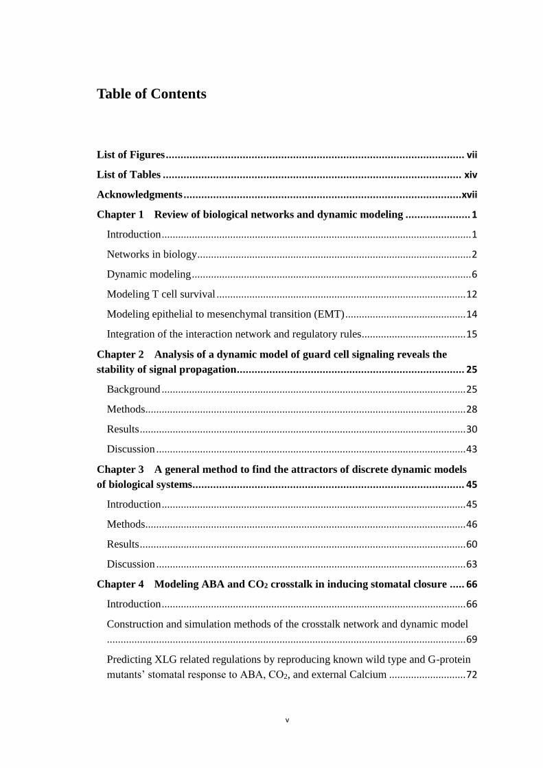
Table of Contents

List of Figures ..................................................................................................... vii

List of Tables ..................................................................................................... xiv

Acknowledgments .............................................................................................. xvii

Chapter 1 Review of biological networks and dynamic modeling ...................... 1

Introduction ................................................................................................................. 1

Networks in biology .................................................................................................... 2

Dynamic modeling ...................................................................................................... 6

Modeling T cell survival ........................................................................................... 12

Modeling epithelial to mesenchymal transition (EMT) ............................................ 14

Integration of the interaction network and regulatory rules...................................... 15

Chapter 2 Analysis of a dynamic model of guard cell signaling reveals the

stability of signal propagation ............................................................................. 25

Background ............................................................................................................... 25

Methods..................................................................................................................... 28

Results ....................................................................................................................... 30

Discussion ................................................................................................................. 43

Chapter 3 A general method to find the attractors of discrete dynamic models

of biological systems............................................................................................ 45

Introduction ............................................................................................................... 45

Methods..................................................................................................................... 46

Results ....................................................................................................................... 60

Discussion ................................................................................................................. 63

Chapter 4 Modeling ABA and CO2 crosstalk in inducing stomatal closure ..... 66

Introduction ............................................................................................................... 66

Construction and simulation methods of the crosstalk network and dynamic model

................................................................................................................................... 69

Predicting XLG related regulations by reproducing known wild type and G-protein

mutants’ stomatal response to ABA, CO2, and external Calcium ............................ 72

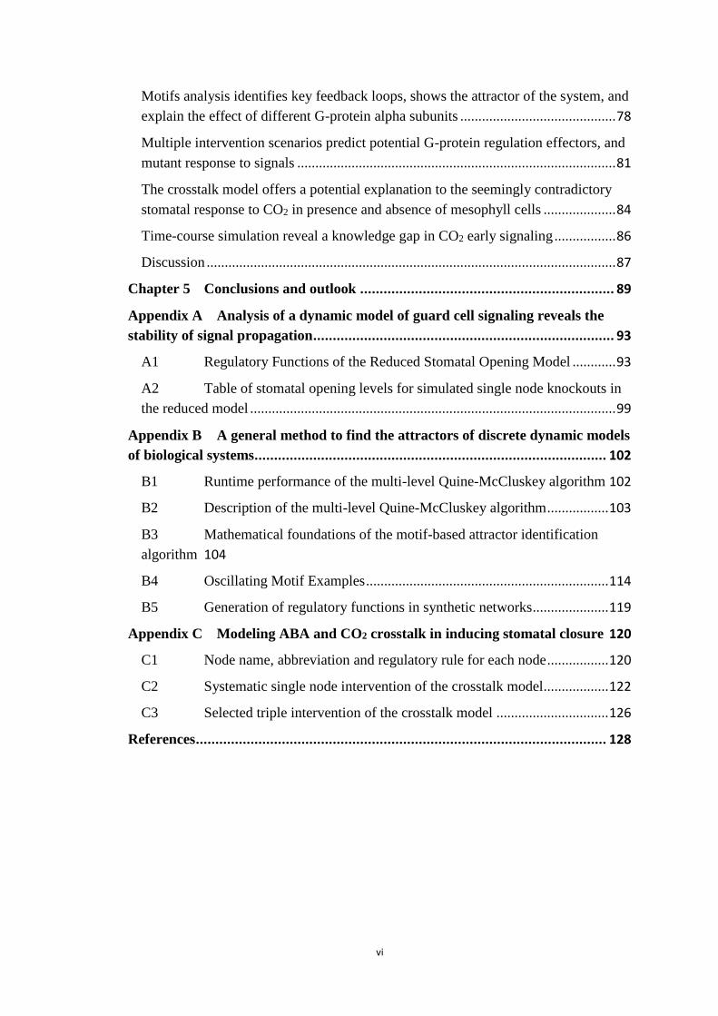
vi

Motifs analysis identifies key feedback loops, shows the attractor of the system, and

explain the effect of different G-protein alpha subunits ........................................... 78

Multiple intervention scenarios predict potential G-protein regulation effectors, and

mutant response to signals ........................................................................................ 81

The crosstalk model offers a potential explanation to the seemingly contradictory

stomatal response to CO2 in presence and absence of mesophyll cells .................... 84

Time-course simulation reveal a knowledge gap in CO2 early signaling ................. 86

Discussion ................................................................................................................. 87

Chapter 5 Conclusions and outlook ................................................................. 89

Appendix A Analysis of a dynamic model of guard cell signaling reveals the

stability of signal propagation ............................................................................. 93

A1 Regulatory Functions of the Reduced Stomatal Opening Model ............ 93

A2 Table of stomatal opening levels for simulated single node knockouts in

the reduced model ..................................................................................................... 99

Appendix B A general method to find the attractors of discrete dynamic models

of biological systems.......................................................................................... 102

B1 Runtime performance of the multi-level Quine-McCluskey algorithm 102

B2 Description of the multi-level Quine-McCluskey algorithm ................. 103

B3 Mathematical foundations of the motif-based attractor identification

algorithm 104

B4 Oscillating Motif Examples ................................................................... 114

B5 Generation of regulatory functions in synthetic networks ..................... 119

Appendix C Modeling ABA and CO2 crosstalk in inducing stomatal closure 120

C1 Node name, abbreviation and regulatory rule for each node ................. 120

C2 Systematic single node intervention of the crosstalk model.................. 122

C3 Selected triple intervention of the crosstalk model ............................... 126

References ......................................................................................................... 128

vii

List of Figures

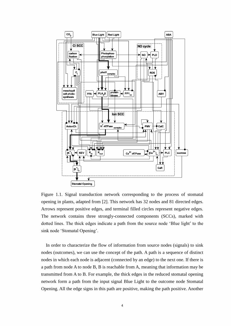
Figure 1.1. Signal transduction network corresponding to the process of stomatal

opening in plants, adapted from [2]. This network has 32 nodes and 81 directed

edges. Arrows represent positive edges, and terminal filled circles represent

negative edges. The network contains three strongly-connected components

(SCCs), marked with dotted lines. The thick edges indicate a path from the

source node ‘Blue light’ to the sink node ‘Stomatal Opening’. ....................... 4

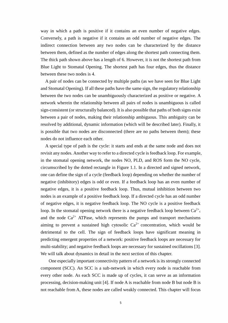
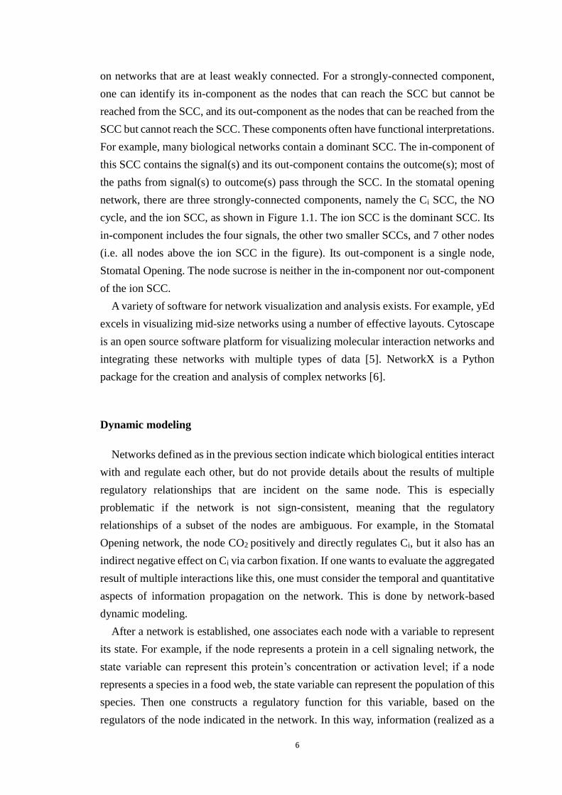
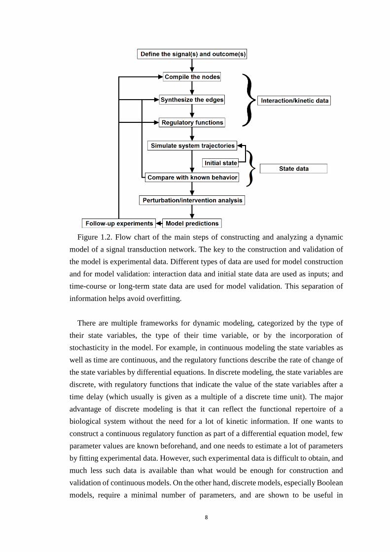
Figure 1.2. Flow chart of the main steps of constructing and analyzing a dynamic

model of a signal transduction network. The key to the construction and

validation of the model is experimental data. Different types of data are used

for model construction and for model validation: interaction data and initial

state data are used as inputs; and time-course or long-term state data are used

for model validation. This separation of information helps avoid overfitting. 8

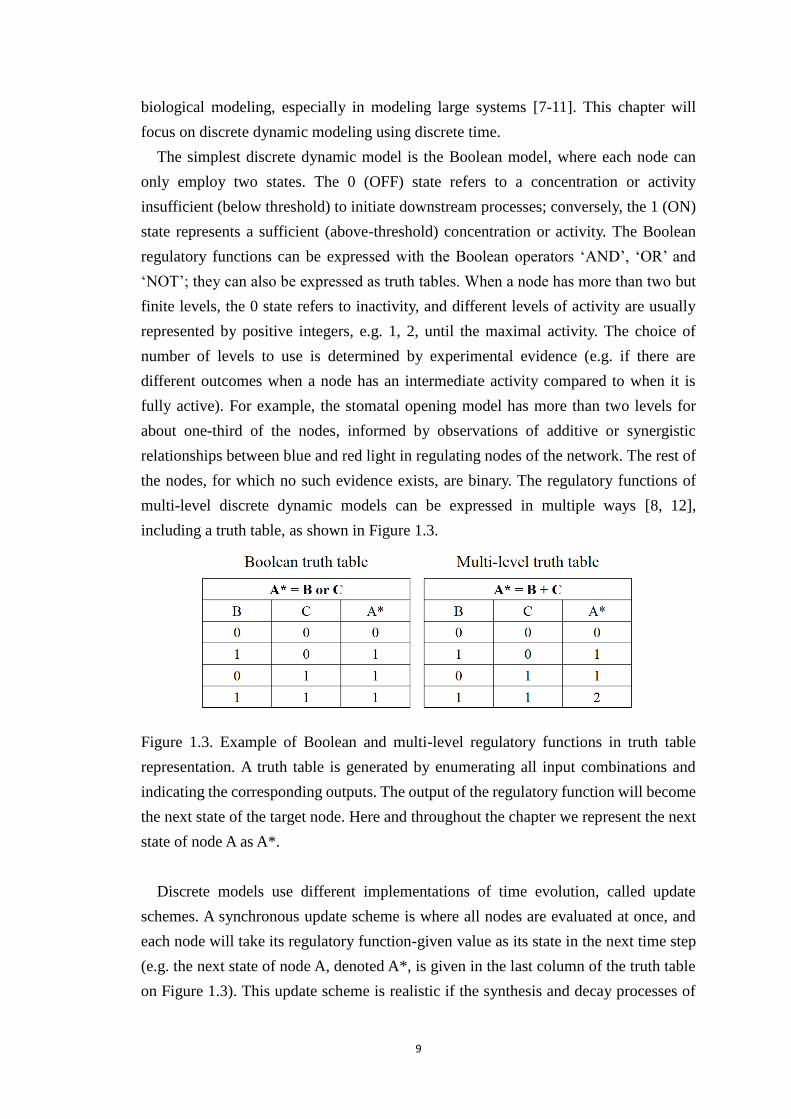
Figure 1.3. Example of Boolean and multi-level regulatory functions in truth table

representation. A truth table is generated by enumerating all input

combinations and indicating the corresponding outputs. The output of the

regulatory function will become the next state of the target node. Here and

throughout the chapter we represent the next state of node A as A*. .............. 9

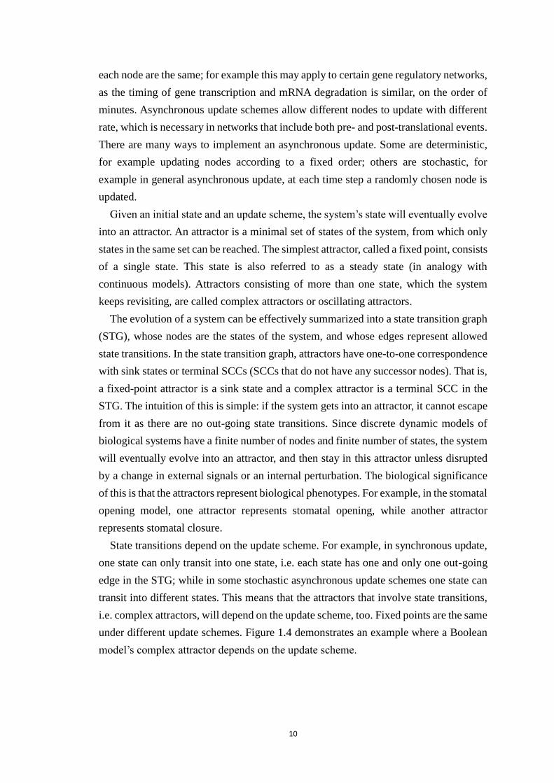
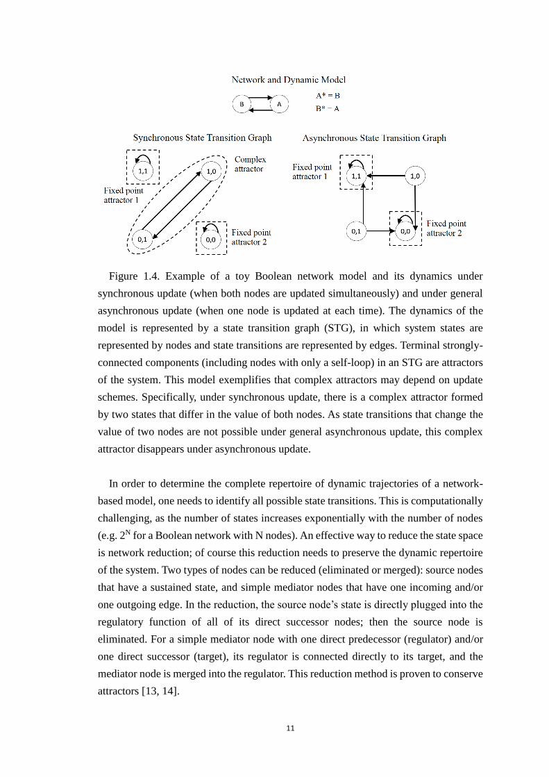
Figure 1.4. Example of a toy Boolean network model and its dynamics under

synchronous update (when both nodes are updated simultaneously) and under

general asynchronous update (when one node is updated at each time). The

dynamics of the model is represented by a state transition graph (STG), in

which system states are represented by nodes and state transitions are

represented by edges. Terminal strongly-connected components (including

nodes with only a self-loop) in an STG are attractors of the system. This model

exemplifies that complex attractors may depend on update schemes.

Specifically, under synchronous update, there is a complex attractor formed

by two states that differ in the value of both nodes. As state transitions that

change the value of two nodes are not possible under general asynchronous

update, this complex attractor disappears under asynchronous update. ........ 11

Figure 1.5. T-LGL survival signaling network by Zhang et al, reproduced with

permission from [22] , copyright (2008) National Academy of Sciences, U.S.A.

The network contains 58 nodes and 123 edges. Up-regulated or constitutively

active nodes are in red, down-regulated or inhibited nodes are in green, nodes

that have been suggested to be deregulated (either up-regulation or down-

regulation) are in blue, and the states of white nodes are unknown or

unchanged compared with normal. Blue edges with arrowheads indicate

activation and red edges that terminate in diamonds indicate inhibition. The

shape of the nodes indicates the cellular location or the corresponding proteins,

transcripts or molecules: rectangles indicate intracellular components, ellipses

indicate extracellular components, and diamonds indicate receptors.

Conceptual nodes (Stimuli, Cytoskeleton signaling, Proliferation, and

viii

Apoptosis) are orange. ................................................................................... 13

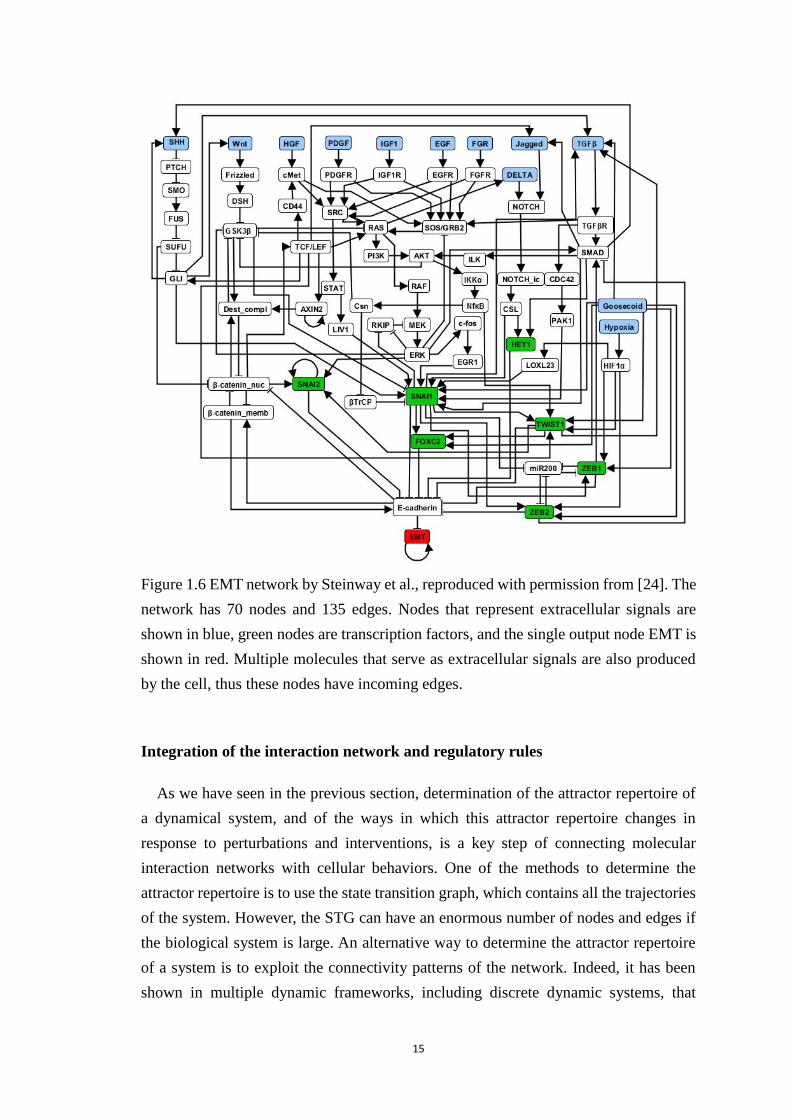
Figure 1.6 EMT network by Steinway et al., reproduced with permission from [24].

The network has 70 nodes and 135 edges. Nodes that represent extracellular

signals are shown in blue, green nodes are transcription factors, and the single

output node EMT is shown in red. Multiple molecules that serve as

extracellular signals are also produced by the cell, thus these nodes have

incoming edges. ............................................................................................. 15

Figure 1.7 Examples of expanded network construction in the Boolean and multi-

level case. Each virtual node is labeled with the state it represents. Each

composite node is black, with a label indicating which node combination it

represents. The complete expanded network is obtained by expanding all

regulatory functions of the original model. ................................................... 17

Figure 1.8. Example of elementary signaling modes (ESMs) in a partial expanded

network. The labeled virtual nodes correspond to the ON state of the respective

nodes in the original signal transduction network; the black node is a

composite node. There are two ESMs in the network: the path A1 B1 D1 E1,

shown as the dotted line, and the subgraph that contains A1, C1, B1, the

composite node, and E1, shown with a dashed line. Each is sufficient for the

signal to activate the outcome. This figure was adapted from [29]. .............. 18

Figure 1.9. Example of stable motif identification from a three-node Boolean

dynamic model. The regulatory functions of the virtual nodes are given. The

black nodes in the expanded network are composite nodes. Three stable motifs

can be identified from the expanded representation of the network. The first

stable motif represents the simultaneous activation (state 1) of nodes A and B.

The second and third stable motifs represent the sustained inactivation (state

0) of A and C, respectively. Notice that a stable motif corresponds to a positive

feedback loop (or SCC) in the original network, but not all positive feedback

loops are stable motifs. .................................................................................. 19

Figure 1.10. Example of attractor identification with iterative stable motif guided

network reduction using the same model as in Figure 1.9. There are three

stable motifs in the model. In the iterative reduction process, each of them is

plugged into the regulatory functions (represented by indicating the stable

motif above an arrow), resulting in a reduced model (indicated by the

interaction network and regulatory functions), where further stable motif

analysis is performed. For simplicity of representation of the A1, B1 stable

motif, we do not show the composite node. When all nodes’ states are

identified in the process, the reduction is complete and an attractor is obtained.

....................................................................................................................... 20

Figure 1.11. Part of the stable motif succession diagram of the T-LGL network,

adapted from [31]. The state of the nodes in each motif is indicated by a

number, separated from the node name by an underscore (e.g. S1P_0

represents S1P at state 0). A stable motif sequence determines the attractor, i.e.

Apoptosis or T-LGL leukemia (cancer). For example, the activation of the

Ceramide=0, S1P=1, PDGFR=1, SPHK1=1 motif leads to the reduction of the

ix

whole network and convergence into the T-LGL leukemia attractor. ............ 21

Figure 1.12. The logic backbone of the EMT model, reproduced from [34]. This is

a condensed version of the EMT network, where each stable motif of the

model is represented by a single node (in blue), and its causal relationships

with the signals and the outcome node EMT (in yellow) are visualized. All

edges are sufficient activations, i.e. the activity (sustained ON state) of the

input node/motif will activate the target node or motif. Any signal, or any

stable motif is sufficient to drive EMT. ......................................................... 22

Figure 1.13. An example ESM from the EMT network, from the signal PDGF to

output EMT. The state of the nodes are marked at the end of each node label

(e.g. PDGF_1 means PDGF at state 1.). The existence of this ESM indicates

that the sustained presence of the PDGF signal alone is sufficient to drive EMT.

Note that this ESM contains three composite nodes. .................................... 22

Figure 1.14. Stable motif associated with the epithelial state in the EMT network

and illustration of control sets that guarantee convergence to the epithelial state,

reproduced from [25]. The entire graph is the epithelial stable motif. Nodes in

black are OFF, and nodes in white are ON. Controlling of one node in each

yellow rectangle, e.g. SMAD, SNAI1, RAS, SHH knockout combined with β-

catenin_memb constitutive activation, ensures convergence to the epithelial

state. The nodes highlighted in blue represent SMAD and the nine nodes

whose knockout in combination with SMAD is able to prevent TGFβ-driven

EMT. The fact that these blue nodes are either part of a yellow rectangle

(SMAD, RAS), on a path that ends in a node of a yellow rectangle (DELTA,

NOTCH, NOTCH_ic, CSL) or on a path that starts with a node of a yellow

rectangle (PI3K, AKT) indicates the inclusive relationship between node sets

whose control prevents or, respectively, reverses EMT. ................................ 24

Figure 2.1 The signal transduction network responsible for stomatal opening, as

reconstructed by Sun et al.[1]. The color of a node marks which signal

regulates this node. Red nodes are regulated solely by red light. Blue nodes

are regulated solely by blue light. Yellow nodes are regulated solely by ABA.

Grey nodes are regulated by CO2. Purple nodes are regulated by both blue and

red light. Green nodes are regulated by blue (and potentially, red) light and

ABA. White nodes are source nodes not regulated by any of the four signals.

To improve visualization, certain pairs of edges with the same starting or end

nodes overlap. Nodes with multiple levels in the dynamic model are

represented by red shadows; the others are Boolean. The full names of the

network components denoted by abbreviated node names are given in Table 1.

This figure and part of its caption is reproduced from Sun Z, Jin X, Albert R,

Assmann SM (2014) Multi-level Modeling of Light-Induced Stomatal

Opening Offers New Insights into Its Regulation by Drought. PLoS Comput

Biol 10(11): e1003930. doi:10.1371/journal.pcbi.1003930. ......................... 26

Figure 2.2 The stomatal opening network after model reduction, with 32 nodes and

81 edges. Nodes with shadows have multiple states; other nodes are binary.

The three strongly-connected components (SCCs) of the network are indicated

x

by rectangles with dashed contours. .............................................................. 33

Figure 2.3 The Ion SCC after reducing all edges that depend on Calcium. All

regulators of this sub-network have been omitted. On the left, [Ca2+]c related

nodes form a sink sub-network. ..................................................................... 39

Figure 3.1 Demonstration of the construction of a quasi-Boolean regulatory

function. A 3-level node A has regulatory function: fA =B+C, where B and C

both have 2 levels. From the truth table, one can identify the regulatory

function for each virtual node of A, by connecting all conjunctive clauses that

yield the same state of A with the Boolean ‘or’ operator. In this way, each

virtual node’s regulatory function will have a Boolean disjunctive normal form.

....................................................................................................................... 49

Figure 3.2 Example of the multi-level Quine-McCluskey algorithm. A Boolean

node D is regulated by a Boolean node A and two 3-state nodes B and C. The

original function of D is shown in a truth table on the top left, in a form

summarizing all input combinations that yield fD(1) =1. The top right table

shows the minterms sorted according to the number of zeros in them. From

this table, one can merge the terms between layers that are different by 1 digit,

if all states of the difference node are present within the two layers. The result

of the merging is shown below. Merged terms are represented by an ‘X’. There

are 5 leftover terms after 1st order merging, and there is 1 leftover term after

0th order merging. The sum of all six terms is the final expression. .............. 51

Figure 3.3 Construction of an expanded network from a regulatory function. Virtual

node A0 has function fA(0) = B0 or (C1 and B1), so in the expanded network,

B0 is connected directly to A0; C1 and B1 are connected indirectly to A0 via

composite node 'C1 and B1'. A1 has function fA(1) = C0 and B1, so C0 and B1

are connected indirectly to A0 via composite node 'C0 and B1'. .................. 52

Figure 3.4 Illustration of stable motif identification in a three-node network. (A)

The original network and the regulatory functions of each node; (B) The

expanded network is constructed according to the steps in sub-section E of

Methods, and then the stable motifs are found by their definition in I.F. (C)

Stable motifs found in this example. The first stable motif, A0, B0,

corresponds to a fixed point attractor of the system A=0, B=0, C=0. The state

C=0 is found by plugging A=B=0 into the regulatory function of C. The 2nd

stable motif corresponds to another fixed point attractor A=2, B=2, C=0. ... 53

Figure 3.5 An example of an oscillating motif in a multi-level network. Panel (A)

shows the network and regulatory functions; panel (B) indicates the expanded

network and motifs. A0 and B0 form a stable motif, indicating a fixed point

A=0, B=0; while A1, A2, B1 and B2 form an oscillating motif, indicating a

possible complex attractor involving states A=1, A=2, B=1 and B=2. Panel (C)

indicates the state transition graph of the system when using general

asynchronous update. The stable motif and oscillating motif identified in 5B

correspond to a fixed point and a complex attractor, respectively................. 55

Figure 3.6 An example of an oscillating motif that contains a stabilized node. (A)

The network and regulatory functions. (B) The expanded network and motifs.

xi

The oscillating motif contains only one virtual node of B, meaning that B will

stabilize at 1 in the complex attractor. (C) The state transition graph using

general asynchronous update. There are two attractors: a fixed point attractor,

and a complex attractor. ................................................................................. 56

Figure 3.7 Attractor identification for a four-node network by a motif succession

diagram. A. The network and the regulatory function of each node. B. Motif

succession diagram. Three motifs are found from the original network,

including 2 stable motifs (A0, B0), (C1, D1), and one oscillating motif (A1,

A2, B1, B2). For each motif, the values of the nodes in the motif are plugged

into the regulatory functions, reducing the network. Then new motifs are

identified from the reduced networks. The sequences corresponding to the

three motifs are labeled (1), (2) and (3). ........................................................ 58

Figure 4.1 The ABA-CO2 crosstalk network. The network has 28 nodes and 58

edges. Nodes with red labels are CO2 related. Red edges are assumed

regulations. Among them, directed red edges are inferred regulations that are

necessary for CO2 induced closure; undirected red edges are based on

observed protein-protein interactions (see the next section for details). The

sole strongly-connect component, marked with “SCC” label, contain 18 nodes.

A table of nodes names and abbreviations can be found in Appendix C1. .... 70

Figure 4.2 Time course simulation of closure in response to ABA, CO2 and external

Calcium signals. The horizontal axis is the simulation time step, and the

vertical axis is the average closure averaged over 1000 simulations. The tiny

peak at time step~1 is due to randomized initial conditions. ......................... 72

Figure 4.3 Two representative edge/regulation settings of the CO2 signaling sub-

network. Substituting this into Figure 4.1 will complete the network. Black

edges are known and red edges are assumptions/predictions. The main

difference between these two network settings is the opposite direction of the

regulatory relationship between XLGs and HT1. .......................................... 77

Figure 4.4 Result of motifs analysis of the crosstalk model. These motifs are shown

in the expanded network representation (described in Chapter 3) here. Node

states are represented by color: grey colored nodes represent nodes in their

OFF states, white colored nodes represent nodes in their ON states. Black

nodes without labels represent a composite node, as combinatorial regulation

(i.e. “AND” logical operation). “Rboh” is the short-hand notation for

“AtRbohD/F”. A&B: stable motifs found in ABA and CO2 signal, respectively.

C. Two stable motifs are found in the absence of any signals: one associated

with closure and the other associated with non-closure. The dotted line means

that either XLG or GPA1 is sufficient to complete the motif. D. two-node

oscillating motif found in all closure ON attractors. The left hand side is the

original network, the right hand side is the motif in expanded network

representation. ................................................................................................ 79

Figure 4.5 Flow chart of activation sequence of components in the network. “CaIM”

is short for Calcium influx through the membrane. “AtRboh stable motif” is

defined in the previous section and can be interpreted as ROS (reactive oxygen

xii

species) production. The ABA response is fastest because ABA early signaling

can activate AtRboh stable motif. External Calcium activates the downstream

of the CO2 signaling pathway directly, and is therefore faster than CO2

signaling. The fact that in experiments CO2 response is fast may suggest a

Calcium independent pathway from CO2 signaling to the downstream, as

indicated in the figure with the dotted edge(s). ............................................. 87

Figure B.1 Histogram of QM transformation runtime on 100 randomly generated

heterogeneous networks with 50 nodes. The result shows that the complexity

of QM transformation is much less than identifying motifs. ....................... 103

Figure B.2 An example of a timing-dependent complex attractor. (A) The network

and regulatory functions. (B) The state transition graph under synchronous

update. Each node of the state transition graph is a state, given in the order A,

B, and each edge is a state transition allowed by synchronous update. The

system has two fixed points, (0,0) and (1,1). It also has a complex attractor

formed by the states (0,1) and (1,0). (C) The state transition graph under

general asynchronous update (i.e. when one node is updated at a time). Only

the two fixed point attractors exist. The synchronous complex attractor is

timing-dependent and does not exist in this update scheme. ....................... 114

Figure B.3 An example of an oscillating motif without a complex attractor. (A) The

network and regulatory functions. (B) The expanded network and motifs.

There is a stable motif formed by A0 and B0, and an oscillating motif made

up by A1, A2, B1. (C) The state transition graph using general asynchronous

update. There is only one attractor, which is a fixed point. The transient

oscillation between states (2,1) and (1,1) will eventually converge into the

fixed point. ................................................................................................... 115

Figure B.4 Examples of stabilized nodes downstream of oscillating node(s). (A) A

Boolean example where A and B oscillate but their downstream C is stable

under that oscillation. (B) The general asynchronous state transition graph of

nodes A and B. The state (A=1,B=1) is not visited in the long term, leading to

the stabilization of C=0. (C) A multi-level example where A is oscillating

between 1 and 2, leading to B stabilizing at 1. This example arises because of

asymmetry in the nodes’ number of states: A has three states but B only has

two states. .................................................................................................... 116

Figure B.5 An example of an unstable oscillation. The system has a fixed point and

a complex attractor. (A) The network and regulatory functions. (B) The

expanded network and motifs. The entire expanded network forms an

oscillating motif, containing the stable motif by two nodes A1, B1, and one

composite node. (C) The state transition graph using general synchronous

update. There is a fixed point attractor A=1, B=1, and a complex attractor.

Note that in the complex attractor, although both A and B are allowed to enter

state 1, they cannot be in state 1 simultaneously. ........................................ 117

Figure B.6 An example of an oscillating motif containing two complex attractors.

(A) The network and regulatory functions. (B) The expanded network and

motifs. The entire expanded network forms an oscillating motif. (C) The state

xiii

transition graph. For simplicity self-loops representing self-transitions are not

shown in the graph. There are two complex attractors, the first attractor is B=0,

A=0 or 1, and the second attractor is B=1, A =2 or 3. ................................. 118

xiv

List of Tables

Table 2.1 Grouping of the stomatal opening values by the level of [K+]v and sucrose

The first two columns indicate the [K+]v and sucrose levels. The third column

is the possible values of stomatal opening in the Sun et al. model for the given

[K+]v and sucrose levels. Note that here we only show [K+]v, sucrose and

stomatal opening value combinations observed in the simulations of the 66

experimentally studied scenarios reported by Sun et al.[1]. More stomatal

opening values are possible when considering node perturbations. The 4th

column shows the simplified stomatal opening level after grouping. The

update function for the simplified stomatal opening level covers all possible

values of [K+]v and sucrose (see Appendix A1). ........................................... 31

Table 2.2 Example of Boolean conversion. The multi-level node shown in the 1st

column is mapped into two Boolean nodes, shown in the 2nd and 3rd columns,

using the binary representation of the corresponding integer. ....................... 35

Table 2.3 Summary of the attractors found using the stable motif algorithm. The

first 5 columns indicate the input signal combination. The setting CO2_high=1

and CO2=0 is not included because it is not biologically meaningful. The “SO

(Bool)” column indicates the state of the Boolean node combination

representing stomatal opening. The “SO” column is the state of stomatal

opening when converted back to an integer. Note that the stomatal opening

level of four is not defined, and no attractors have a stomatal opening level of

two. The next column indicates whether Ca2+ oscillation can possibly happen

under the given signal combination. The last column indicates whether

bistability of PMV_pos can be observed under this setting. In those cases, two

stable steady states with (PMV_pos=0, Kout=0) and (PMV_pos=1, Kout=1) can

be observed. The rest of the nodes are unaffected by this two-node bistability.

....................................................................................................................... 36

Table 2.4 Summary of systematic perturbation results. The first set of columns, with

the header ‘Light, CO2 and ABA condition’, indicate the input signal

combinations. The abbreviation “Mod.” means moderate CO2 concentration.

Note that we do not list the four input combinations (high CO2 with ABA and

with any type of light, or moderate CO2 with ABA and red light) wherein all

simulated stomatal opening values are zero. The 2nd column is the simulated

stomatal opening (SO) level in the unperturbed system. The 3rd column set

shows the percentage of single-node knockouts that yield the corresponding

SO level. There is no stomatal opening level 4 in the reduced model. No entry

means zero percentage. The last column is the percentage of settings where

the stomatal opening remains at the same level as the unperturbed case. A

complete table of perturbation results is provided in Appendix A2. ............. 41

Table 2.5 Nodes whose knockouts diminish ABA’s inhibition of stomatal opening.

The first set of columns, with the header ‘Light, CO2 and ABA condition’,

indicate the input signal combinations. The 2nd column is the stomatal opening

xv

without perturbations. The 3rd column set indicates the nodes whose knockout

would yield a stomatal opening level that is higher than the unperturbed value

of 0. CO2 knockout means CO2 being set to zero (CO2 free air). No entry

means the setting does not cause partial reversal. ......................................... 44

Table 3.1 Benchmark runtime of the motif-based algorithm on synthetic networks

of different sizes (number of nodes). For each size, 50-100 random networks

with in-degree k=2 are generated. For multi-level networks, each node has 50%

chance of having 2 levels and has 50% chance of having 3 levels. In all runs,

the attractors found by the algorithm are identical or highly consistent with the

attractors found with the sampling method. .................................................. 61

Table 3.2 Summary of the runtime of the two algorithms. The networks fall into

three categories. The first column is the number of networks in each category.

The second column is the range of the network sizes in each category. The 3rd

and 4th columns indicate whether motif analysis and GINsim STG/HTG

generation was successfully completed or not. For completed analysis, the

range of computational time is shown in the table. Otherwise, we indicate

DNC (meaning “did not complete”), which includes cases that ran out of

memory or did not finish in 6 hours. All tests were run on a personal computer.

There is no model where GINsim succeeds and the motif-based algorithm fails.

The motif algorithm is successful in 18 of 19 models, while GINsim

STG/HTG only works in the small networks of the first category. ............... 63

Table 4.1 Simulation of the closure pattern compared with experimental

observation. The first two columns indicate the status of the ABA and CO2

signal. The third column is the intervention applied to the system. External

Calcium is a treatment; XLG and GPA KO represent the xlg triple mutant or

gpa1 mutant, respectively. The “Observed” column indicates the qualitative

outcome of the experiments. “Closure” indicates a significantly decreased

stomatal aperture compared to the control setting that lacks any signal or

intervention. “Loss of closure” indicates that the relevant intervention causes

a substantial decrease in the effect of the relevant signal, thus the combined

outcome of the signal and intervention is closer to the control (no closure) than

to the effect of the signal alone (closure). The “Simulation” column records

the simulated closure value at the end of the simulation (i.e. after 40 time steps)

under each condition, averaged over 100 simulations. A value less than 1 in

the simulation column is consistent with a loss of closure. The table shows that

the model reproduces experimental observations. Notation “KO” means

knockout. ....................................................................................................... 73

Table 4.2 closure response to interventions of early CO2 signaling components. The

first row is experimental observation of closure response, and the second row

is the model simulation. Additional edges (e.g. RHC1 XLGs) are required

to make the two rows consistent. ................................................................... 76

Table 4.3 example of single node intervention. The number is the closure value after

50 time steps, averaged over 500 simulations. This set of simulations predicts

that ROS treatment can restore loss of closure in xlg triple mutants or

xvi

atrbohD/F mutants. ....................................................................................... 81

Table 4.4 Selected double interventions under each signal: A. External Ca2+; B. CO2;

C. ABA. Each row is a genotype (wildtype or the indicated mutant), and each

column is a treatment (including no special treatment). All simulated closure

values are reported after 50 time steps, averaged over 500 simulations.

Yellowed slots are those that display a significantly different value compared

with no treatment. Conclusion on the observations in the row/column are

located on the last column/row of each sub-table. ......................................... 84

Table 4.5 Simulation on closure response to CO2 without or with the ‘mesophyll

signal’ node, together with the assumption that mesophyll produces ABA. . 86

Table A.1 Full names of the network components denoted by abbreviated node

names in Figure 2.1. The same abbreviations are used in the original Sun et al.

model and the reduced model. ....................................................................... 95

Table A.2 Stomatal opening levels for simulated single node knockouts in the

reduced model .............................................................................................. 101

xvii

Acknowledgments

The research described in this dissertation was supported by the National Science

Foundation grants NSF IIS 1161007, NSF PHY 1205840, NSF PHY 1545832, NSF

MCB 1715826. The findings and conclusions do not necessarily reflect the view of the

funding agency.

I would like to thank my advisor, Dr. Réka Albert, for her exemplary expertise and

professionalism, for her extensive mentoring, and for her firm support throughout my

Ph.D. career. I thank the committee members, Dr. Carina Curto, Dr. Dezhe Jin, Dr. Sarah

M. Assmann, plus Dr. John Fricks and Dr. Costas D. Maranas as former committee

members. I would also like to thank Dr. Colin Campbell, Dr. Zhongyao Sun, Dr. Sarah.

M. Assmann, Dr. Jorge G.T. Zañudo, Dr. Gang Yang, Dr. István Albert, Nianyuan Bao,

Parul Maheshwari, Jordan Rozum, Dr. David Chakravorty, Dr. Palanivelu Sengottaiyan,

Dr. Yotam Zait, Dr. David Wooten and Dávid Deritei for helpful discussions related to

my projects.

1

Chapter 1 Review of biological networks

and dynamic modeling

The content of this chapter is based on a book chapter “Modeling biological information

processing networks” where I am the first author. The book chapter has been submitted

to the book Physics of Molecular and Cellular Systems, edited by Krastan B. Blagoev

and Herbert Levine. A subset of the figures are reproduced in this chapter.

Introduction

Interacting systems abound at every level of biological organization (molecular,

cellular, organ, organism or population). For example, molecular interacting systems

consist of genes, their transcripts (mRNAs), proteins, small molecules; their interactions

include gene transcription, protein translation, protein-protein interactions and chemical

reactions. A fundamental goal of biology is to understand why biological systems

behave the way they do. One promising avenue toward this goal is to realize that

interacting biological systems at each level can determine the behavior at the next level.

For example, cellular decisions, behaviors, and phenotypes arise from the interactions

of numerous molecular components. Similarly, interactions among cells determine how

multi-cellular organisms develop and how tissues and organs function; interactions

among individuals form the basis of social communities; and interactions among species

underlie ecological communities.

A higher-level function, behavior, or phenotype is an emergent property that arises

from the totality of the lower-level elements and interactions. That is, one usually cannot

attribute a cell behavior to a single gene or protein. This does not necessarily mean,

however, that all the elements and interactions are equally important in determining a

higher-level behavior. Biological networks offer a visual and effective way to represent

the lower level elements and interactions; the analysis of these networks is a key step

toward the elucidation of higher-level emergent properties. Specifically, network

analysis and network-based dynamic modeling can be used to determine the repertoire

of cellular behaviors associated to a within-cell network, and to identify the sub-

networks that play a key role in the cell adopting a certain behavior.

Another aspect of understanding biology is that, despite the vast amounts of recent

information about regulatory relationships among genes, proteins, and small molecules,

2

many knowledge gaps still exist. Networks and network-based modeling can integrate

fragmentary and qualitative interaction information, and can make powerful predictions

about undiscovered biology.

In this chapter we focus on the application of network-related methods and techniques

in understanding biology. A variety of networks can be defined at the cellular,

organismal and ecosystem levels. The examples in this chapter will focus on the

molecular to cellular level. We aim to illustrate how to connect the properties of within-

cell information processing networks to cellular phenotypes. We start by introducing

network concepts and measures such as paths, cycles and strongly-connected

components, and their biological interpretation. Then we introduce network-based

dynamic modeling, which offers in-depth insights into dynamical processes and the

effect of perturbations. We describe the construction of dynamic models, and

demonstrate their predictive power through two examples. We also introduce

methodologies that reveal structure-dynamics connections through the construction of

so-called expanded networks.

Networks in biology

A network (also called graph) consists of nodes (also called vertices) and edges that

connect pairs of nodes. In a biological network, nodes represent biological elements, for

example proteins and molecules in a cell signaling process; edges represent interactions

or regulatory effects between these elements. The edges of a network may be directed

or undirected. An undirected edge connects a node pair without order, that is, edge (x,

y) is identical to edge (y, x). For a directed edge the order of the node pair matters: a

directed edge (x, y) starts from x and ends in y. One can refer to x as the head or source

of the edge and refer to y as the tail or target of the edge; y is also said to be a direct

successor of x and x is said to be a direct predecessor of y. Edges can also be

characterized by positive or negative signs. In biological networks, the sign of an edge

represents the effect of the regulation. A positive edge stands for positive regulation (i.e.,

activation); a negative edge stands for negative regulation (i.e., inhibition). Biological

networks are often directed and signed; this way the network is a reflection of the flow

of mass and information in the system. During the construction of the network, certain

nodes may be designated as markers or proxies for higher-level behavior. For example,

certain genes or proteins can be used as markers of cell types (as it is also done in

experimental investigation), and abstract nodes can be added as proxies of the

phenotypic outcome of a signal transduction network.

We use as first illustration a signal transduction network inside plant guard cells. This

3

network will be described in more detail in Chapter 2. Guard cells border the stomata,

which are pores on leaf surfaces that allow the plant to exchange carbon dioxide (CO2)

and oxygen with the atmosphere. The shape change of the guard cells determines

stomatal opening (increased aperture) or closure. This shape change is elicited by

environmental signals, including light of different wavelength, CO2 concentration, as

well as internal signals (hormones) such as abscisic acid (ABA). Thus, the within-guard

cell signal transduction network can be defined as the elements and interactions that

respond to the external and internal signals and yield stomatal opening (or closure). Sun

et al. constructed a signaling network of light-induced stomatal opening, which

contained more than 70 nodes and 150 directed and signed edges [1]. Figure 1.1 shows

a reduced version of this network, with 32 nodes, including the outcome node Stomatal

Opening, and 81 edges [2].

The organizational features of a network reflect the properties that are critical for

emergent behavior. One way to connect the micro-scale (node) properties to the macro-

scale (network) properties is to look at the connectivity patterns of a network. First, one

can analyze the patterns of how the edges are distributed among nodes. A local measure

of this is the node degree, which in directed networks can be separated into in- and out-

degree. The in-degree of a node is the number of its incoming edges; the out-degree of

a node is the number of its outgoing edges. Nodes with a high in-degree have many

regulators and nodes with a high out-degree regulate many other nodes. A node can also

have a high degree (sum of in-and out-degree) by having intermediary values of in- and

out-degree. All of these types of high-degree nodes (also called hub nodes) have

biological meaning.

A node with only outgoing edges and no incoming edges is called a source node.

These nodes represent external signals. A node with only incoming edges and no

outgoing edges is called a sink node; these nodes represent outcomes of the network. In

the reduced stomatal opening network there are four source nodes, each representing a

signal, namely CO2, Blue Light, Red Light and ABA. There is a single sink node,

Stomatal Opening. The highest-degree (hub) nodes include AnionCh (referring to

multiple anion channels) with in-degree 6 and out-degree 2; and [Ca2+]c (cytosolic Ca2+

concentration) with in-degree 4 and out-degree 7.

4

Figure 1.1. Signal transduction network corresponding to the process of stomatal

opening in plants, adapted from [2]. This network has 32 nodes and 81 directed edges.

Arrows represent positive edges, and terminal filled circles represent negative edges.

The network contains three strongly-connected components (SCCs), marked with

dotted lines. The thick edges indicate a path from the source node ‘Blue light’ to the

sink node ‘Stomatal Opening’.

In order to characterize the flow of information from source nodes (signals) to sink

nodes (outcomes), we can use the concept of the path. A path is a sequence of distinct

nodes in which each node is adjacent (connected by an edge) to the next one. If there is

a path from node A to node B, B is reachable from A, meaning that information may be

transmitted from A to B. For example, the thick edges in the reduced stomatal opening

network form a path from the input signal Blue Light to the outcome node Stomatal

Opening. All the edge signs in this path are positive, making the path positive. Another

5

way in which a path is positive if it contains an even number of negative edges.

Conversely, a path is negative if it contains an odd number of negative edges. The

indirect connection between any two nodes can be characterized by the distance

between them, defined as the number of edges along the shortest path connecting them.

The thick path shown above has a length of 6. However, it is not the shortest path from

Blue Light to Stomatal Opening. The shortest path has four edges, thus the distance

between these two nodes is 4.

A pair of nodes can be connected by multiple paths (as we have seen for Blue Light

and Stomatal Opening). If all these paths have the same sign, the regulatory relationship

between the two nodes can be unambiguously characterized as positive or negative. A

network wherein the relationship between all pairs of nodes is unambiguous is called

sign-consistent (or structurally balanced). It is also possible that paths of both signs exist

between a pair of nodes, making their relationship ambiguous. This ambiguity can be

resolved by additional, dynamic information (which will be described later). Finally, it

is possible that two nodes are disconnected (there are no paths between them); these

nodes do not influence each other.

A special type of path is the cycle: it starts and ends at the same node and does not

revisit any nodes. Another way to refer to a directed cycle is feedback loop. For example,

in the stomatal opening network, the nodes NO, PLD, and ROS form the NO cycle,

circumscribed by the dotted rectangle in Figure 1.1. In a directed and signed network,

one can define the sign of a cycle (feedback loop) depending on whether the number of

negative (inhibitory) edges is odd or even. If a feedback loop has an even number of

negative edges, it is a positive feedback loop. Thus, mutual inhibition between two

nodes is an example of a positive feedback loop. If a directed cycle has an odd number

of negative edges, it is negative feedback loop. The NO cycle is a positive feedback

loop. In the stomatal opening network there is a negative feedback loop between Ca2+c

and the node Ca2+ ATPase, which represents the pumps and transport mechanisms

aiming to prevent a sustained high cytosolic Ca2+ concentration, which would be

detrimental to the cell. The sign of feedback loops have significant meaning in

predicting emergent properties of a network: positive feedback loops are necessary for

multi-stability; and negative feedback loops are necessary for sustained oscillations [3].

We will talk about dynamics in detail in the next section of this chapter.

One especially important connectivity pattern of a network is its strongly connected

component (SCC). An SCC is a sub-network in which every node is reachable from

every other node. As each SCC is made up of cycles, it can serve as an information

processing, decision-making unit [4]. If node A is reachable from node B but node B is

not reachable from A, these nodes are called weakly connected. This chapter will focus

6

on networks that are at least weakly connected. For a strongly-connected component,

one can identify its in-component as the nodes that can reach the SCC but cannot be

reached from the SCC, and its out-component as the nodes that can be reached from the

SCC but cannot reach the SCC. These components often have functional interpretations.

For example, many biological networks contain a dominant SCC. The in-component of

this SCC contains the signal(s) and its out-component contains the outcome(s); most of

the paths from signal(s) to outcome(s) pass through the SCC. In the stomatal opening

network, there are three strongly-connected components, namely the Ci SCC, the NO

cycle, and the ion SCC, as shown in Figure 1.1. The ion SCC is the dominant SCC. Its

in-component includes the four signals, the other two smaller SCCs, and 7 other nodes

(i.e. all nodes above the ion SCC in the figure). Its out-component is a single node,

Stomatal Opening. The node sucrose is neither in the in-component nor out-component

of the ion SCC.

A variety of software for network visualization and analysis exists. For example, yEd

excels in visualizing mid-size networks using a number of effective layouts. Cytoscape

is an open source software platform for visualizing molecular interaction networks and

integrating these networks with multiple types of data [5]. NetworkX is a Python

package for the creation and analysis of complex networks [6].

Dynamic modeling

Networks defined as in the previous section indicate which biological entities interact

with and regulate each other, but do not provide details about the results of multiple

regulatory relationships that are incident on the same node. This is especially

problematic if the network is not sign-consistent, meaning that the regulatory

relationships of a subset of the nodes are ambiguous. For example, in the Stomatal

Opening network, the node CO2 positively and directly regulates Ci, but it also has an

indirect negative effect on Ci via carbon fixation. If one wants to evaluate the aggregated

result of multiple interactions like this, one must consider the temporal and quantitative

aspects of information propagation on the network. This is done by network-based

dynamic modeling.

After a network is established, one associates each node with a variable to represent

its state. For example, if the node represents a protein in a cell signaling network, the

state variable can represent this protein’s concentration or activation level; if a node

represents a species in a food web, the state variable can represent the population of this

species. Then one constructs a regulatory function for this variable, based on the

regulators of the node indicated in the network. In this way, information (realized as a

7

state change of a node) propagates through the network. Each node’s state will evolve

over time, eventually converging into a long-term behavior such as a steady state or a

sustained oscillation. The phenotype of the system can then be characterized by the

long-term state of all nodes, or of a subset of the nodes. For example, if there is a sink

node that represents a phenotypic outcome, the long-term state of this node may be a

sufficient proxy to describe the whole system.

To construct a dynamic model, the modeler needs to start from identifying the process

to be modeled, which will specify the signals and outcomes of the network. Next is to

identify the additional nodes involved in the process, and the interactions among them.

Experimental interaction data, such as physical interactions, chemical reactions, post-

translational modifications, causal effects of knockouts, are used in this process. Then

the regulatory function for each node needs to be determined, and is usually

parameterized using experimental interaction data. In the vast majority of cases, there

isn’t enough information to fully characterize and parameterize each regulatory function.

Once a model is established, one can validate it by simulating the model and

comparing the results with experimental data. A simulation starts at an initial state that

represents the resting (pre-stimulus) status of the system, and it identifies the

consecutive states by applying the regulatory functions. The simulation result should

agree with the experimentally known response of the system to the signal(s).

Intervention or perturbation scenarios can also be simulated and analyzed. Comparing

the model’s results with existing experimental results in these scenarios is an additional

test of the model. If there are discrepancies, one or more regulatory functions need to

be adjusted until a reasonable percentage of simulations is consistent with experiments.

This adjustment process decreases the uncertainty of the regulatory functions.

After the model is validated, it can be used to make predictions about situations that

were not studied before. For example, the model can identify key nodes, whose

perturbation disrupts a certain behavior of the system. If this behavior is undesired, (e.g.

it represents uncontrolled growth of cancer cells) these key nodes serve as intervention

targets. The model’s predictions should be tested by follow-up experiments, which may

confirm the predictions or contradict them. Both cases represent a gain of knowledge.

An invalidated prediction spurs further revisions and increased certainty to the

regulatory functions. Figure 1.2 presents a flow chart of the modeling process.

8

Figure 1.2. Flow chart of the main steps of constructing and analyzing a dynamic

model of a signal transduction network. The key to the construction and validation of

the model is experimental data. Different types of data are used for model construction

and for model validation: interaction data and initial state data are used as inputs; and

time-course or long-term state data are used for model validation. This separation of

information helps avoid overfitting.

There are multiple frameworks for dynamic modeling, categorized by the type of

their state variables, the type of their time variable, or by the incorporation of

stochasticity in the model. For example, in continuous modeling the state variables as

well as time are continuous, and the regulatory functions describe the rate of change of

the state variables by differential equations. In discrete modeling, the state variables are

discrete, with regulatory functions that indicate the value of the state variables after a

time delay (which usually is given as a multiple of a discrete time unit). The major

advantage of discrete modeling is that it can reflect the functional repertoire of a

biological system without the need for a lot of kinetic information. If one wants to

construct a continuous regulatory function as part of a differential equation model, few

parameter values are known beforehand, and one needs to estimate a lot of parameters

by fitting experimental data. However, such experimental data is difficult to obtain, and

much less such data is available than what would be enough for construction and

validation of continuous models. On the other hand, discrete models, especially Boolean

models, require a minimal number of parameters, and are shown to be useful in

9

biological modeling, especially in modeling large systems [7-11]. This chapter will

focus on discrete dynamic modeling using discrete time.

The simplest discrete dynamic model is the Boolean model, where each node can

only employ two states. The 0 (OFF) state refers to a concentration or activity

insufficient (below threshold) to initiate downstream processes; conversely, the 1 (ON)

state represents a sufficient (above-threshold) concentration or activity. The Boolean

regulatory functions can be expressed with the Boolean operators ‘AND’, ‘OR’ and

‘NOT’; they can also be expressed as truth tables. When a node has more than two but

finite levels, the 0 state refers to inactivity, and different levels of activity are usually

represented by positive integers, e.g. 1, 2, until the maximal activity. The choice of

number of levels to use is determined by experimental evidence (e.g. if there are

different outcomes when a node has an intermediate activity compared to when it is

fully active). For example, the stomatal opening model has more than two levels for

about one-third of the nodes, informed by observations of additive or synergistic

relationships between blue and red light in regulating nodes of the network. The rest of

the nodes, for which no such evidence exists, are binary. The regulatory functions of

multi-level discrete dynamic models can be expressed in multiple ways [8, 12],

including a truth table, as shown in Figure 1.3.

Figure 1.3. Example of Boolean and multi-level regulatory functions in truth table

representation. A truth table is generated by enumerating all input combinations and

indicating the corresponding outputs. The output of the regulatory function will become

the next state of the target node. Here and throughout the chapter we represent the next

state of node A as A*.

Discrete models use different implementations of time evolution, called update

schemes. A synchronous update scheme is where all nodes are evaluated at once, and

each node will take its regulatory function-given value as its state in the next time step

(e.g. the next state of node A, denoted A*, is given in the last column of the truth table

on Figure 1.3). This update scheme is realistic if the synthesis and decay processes of

10

each node are the same; for example this may apply to certain gene regulatory networks,

as the timing of gene transcription and mRNA degradation is similar, on the order of

minutes. Asynchronous update schemes allow different nodes to update with different

rate, which is necessary in networks that include both pre- and post-translational events.

There are many ways to implement an asynchronous update. Some are deterministic,

for example updating nodes according to a fixed order; others are stochastic, for

example in general asynchronous update, at each time step a randomly chosen node is

updated.

Given an initial state and an update scheme, the system’s state will eventually evolve

into an attractor. An attractor is a minimal set of states of the system, from which only

states in the same set can be reached. The simplest attractor, called a fixed point, consists

of a single state. This state is also referred to as a steady state (in analogy with

continuous models). Attractors consisting of more than one state, which the system

keeps revisiting, are called complex attractors or oscillating attractors.

The evolution of a system can be effectively summarized into a state transition graph

(STG), whose nodes are the states of the system, and whose edges represent allowed

state transitions. In the state transition graph, attractors have one-to-one correspondence

with sink states or terminal SCCs (SCCs that do not have any successor nodes). That is,

a fixed-point attractor is a sink state and a complex attractor is a terminal SCC in the

STG. The intuition of this is simple: if the system gets into an attractor, it cannot escape

from it as there are no out-going state transitions. Since discrete dynamic models of

biological systems have a finite number of nodes and finite number of states, the system

will eventually evolve into an attractor, and then stay in this attractor unless disrupted

by a change in external signals or an internal perturbation. The biological significance

of this is that the attractors represent biological phenotypes. For example, in the stomatal

opening model, one attractor represents stomatal opening, while another attractor

represents stomatal closure.

State transitions depend on the update scheme. For example, in synchronous update,

one state can only transit into one state, i.e. each state has one and only one out-going

edge in the STG; while in some stochastic asynchronous update schemes one state can

transit into different states. This means that the attractors that involve state transitions,

i.e. complex attractors, will depend on the update scheme, too. Fixed points are the same

under different update schemes. Figure 1.4 demonstrates an example where a Boolean

model’s complex attractor depends on the update scheme.

11

Figure 1.4. Example of a toy Boolean network model and its dynamics under

synchronous update (when both nodes are updated simultaneously) and under general

asynchronous update (when one node is updated at each time). The dynamics of the

model is represented by a state transition graph (STG), in which system states are

represented by nodes and state transitions are represented by edges. Terminal strongly-

connected components (including nodes with only a self-loop) in an STG are attractors

of the system. This model exemplifies that complex attractors may depend on update

schemes. Specifically, under synchronous update, there is a complex attractor formed

by two states that differ in the value of both nodes. As state transitions that change the

value of two nodes are not possible under general asynchronous update, this complex

attractor disappears under asynchronous update.

In order to determine the complete repertoire of dynamic trajectories of a network-

based model, one needs to identify all possible state transitions. This is computationally

challenging, as the number of states increases exponentially with the number of nodes

(e.g. 2N for a Boolean network with N nodes). An effective way to reduce the state space

is network reduction; of course this reduction needs to preserve the dynamic repertoire

of the system. Two types of nodes can be reduced (eliminated or merged): source nodes

that have a sustained state, and simple mediator nodes that have one incoming and/or

one outgoing edge. In the reduction, the source node’s state is directly plugged into the

regulatory function of all of its direct successor nodes; then the source node is

eliminated. For a simple mediator node with one direct predecessor (regulator) and/or

one direct successor (target), its regulator is connected directly to its target, and the

mediator node is merged into the regulator. This reduction method is proven to conserve

attractors [13, 14].

12

A variety of software exist to facilitate discrete dynamical modeling. Model and

software development efforts are coordinated by the Consortium of Logical Models and

Tools (CoLoMoTo), an international open community that aims to develop standards

for model representation and interchange, establish criteria for the comparison of

methods, models and tools and to promote these methods, tools and models [15].

CoLoMoTo members have developed the Qualitative Models Package (“qual”) of the

Systems Biology Markup Language (SBML) [16]. The Cell Collective is a web-based

platform that enables collective model construction and real-time model simulation [17];

GINsim allows asynchronous and/or multi-level dynamics and STG construction [18].

The Python library BooleanNet allows simulation of Boolean models with different

update schemes [19]; SimBoolNet is a Cytoscape app that benefits from the

functionalities and friendly graphic user interface of Cytoscape [20]; the R package

BoolNet can construct and simulate Boolean models and analyze attractors using

exhaustive or heuristic search methods [21].

In the following we present two published models to demonstrate the power of

dynamical modeling of biological networks.

Modeling T cell survival

This model reflects the survival and proliferation of cytotoxic T cells in the context

of the disease T-LGL leukemia. Cytotoxic T cells are generated to fight an infection by

eliminating infected cells, and after the infection is over they usually undergo the

process of activation induced cell death. However in T-LGL leukemia they survive,

adopt a cell state different both from resting and from activated T cells, and start

attacking healthy cells. Zhang et al. synthesized the pathways involved in activation

induced cell death, cell proliferation, as well as the pathways that are known to be

different in T-LGL cells compared to normal cytotoxic T cells (Figure 1.5) [22]. They

formulated a Boolean model of the process and simulated its trajectories, starting from

a just-stimulated T cell, using stochastic timing. The model reproduces the survival of

a fraction of the initial stimulated cells and the known markers of this process, for

example the activation of JAK in every surviving cell. The model has two fixed points:

the normal fixed point that corresponds to programmed cell death, and the disease fixed

point that reproduces the T-LGL survival state. The model predicts that a small subset

of the known deregulations (abnormal node states) is sufficient to cause all the others,

thus preventative efforts should focus on this subset. The model predicts 12 additional

nodes whose state stabilizes in the T-LGL state. The model also predicts several key

nodes whose state change can ensure the apoptosis of the whole population; these key

nodes are potential therapeutic targets for T-LGL leukemia. Several of these predictions

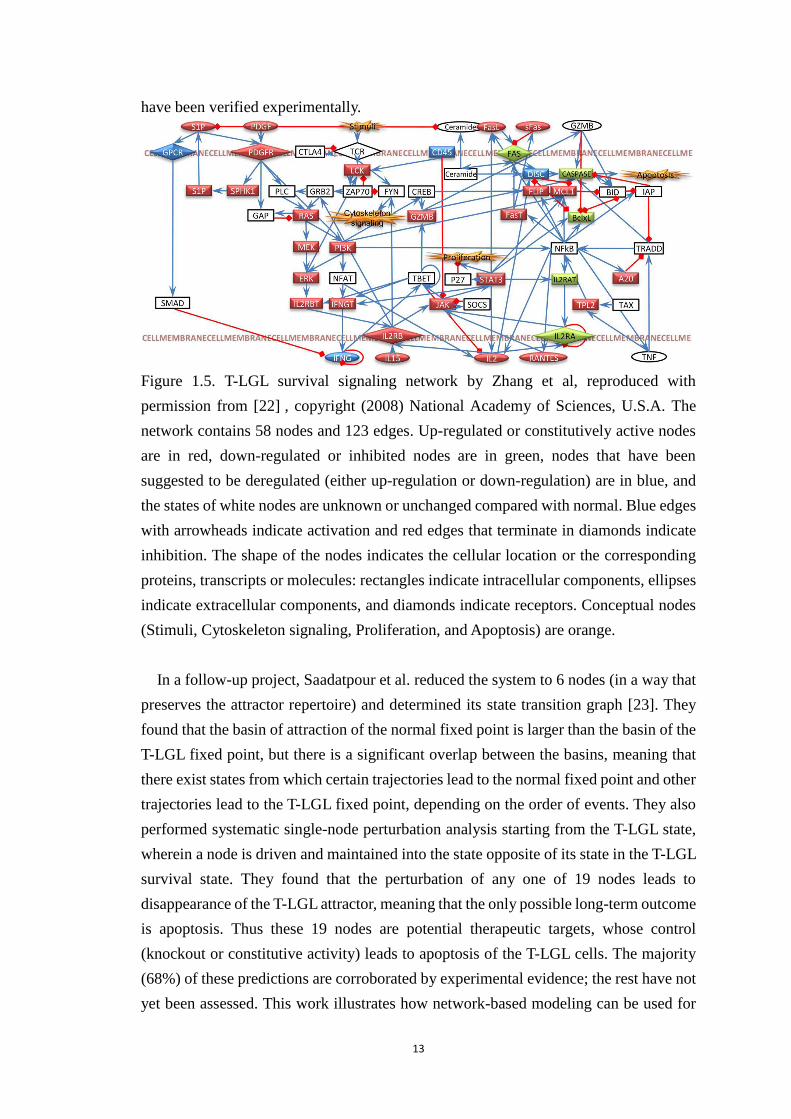
13

have been verified experimentally.

Figure 1.5. T-LGL survival signaling network by Zhang et al, reproduced with

permission from [22] , copyright (2008) National Academy of Sciences, U.S.A. The

network contains 58 nodes and 123 edges. Up-regulated or constitutively active nodes

are in red, down-regulated or inhibited nodes are in green, nodes that have been

suggested to be deregulated (either up-regulation or down-regulation) are in blue, and

the states of white nodes are unknown or unchanged compared with normal. Blue edges

with arrowheads indicate activation and red edges that terminate in diamonds indicate

inhibition. The shape of the nodes indicates the cellular location or the corresponding

proteins, transcripts or molecules: rectangles indicate intracellular components, ellipses

indicate extracellular components, and diamonds indicate receptors. Conceptual nodes

(Stimuli, Cytoskeleton signaling, Proliferation, and Apoptosis) are orange.

In a follow-up project, Saadatpour et al. reduced the system to 6 nodes (in a way that

preserves the attractor repertoire) and determined its state transition graph [23]. They

found that the basin of attraction of the normal fixed point is larger than the basin of the

T-LGL fixed point, but there is a significant overlap between the basins, meaning that

there exist states from which certain trajectories lead to the normal fixed point and other

trajectories lead to the T-LGL fixed point, depending on the order of events. They also

performed systematic single-node perturbation analysis starting from the T-LGL state,

wherein a node is driven and maintained into the state opposite of its state in the T-LGL

survival state. They found that the perturbation of any one of 19 nodes leads to

disappearance of the T-LGL attractor, meaning that the only possible long-term outcome

is apoptosis. Thus these 19 nodes are potential therapeutic targets, whose control

(knockout or constitutive activity) leads to apoptosis of the T-LGL cells. The majority

(68%) of these predictions are corroborated by experimental evidence; the rest have not

yet been assessed. This work illustrates how network-based modeling can be used for

14

predictions that can potentially lead to new therapeutic targets.

Modeling epithelial to mesenchymal transition (EMT)

The epithelial to mesenchymal transition (EMT) is the process where epithelial cells

lose their cell polarity and cell-cell adhesion, and gain migratory and invasive properties,

to ultimately become mesenchymal cells. The loss of the expression of the protein E-

cadherin is considered the hallmark of the EMT transition. This cell fate change is

beneficial during embryonic development and wound healing, but it also is the first step

of cancer metastasis. Steinway et al. constructed a signal transduction network and

Boolean model of this process (Figure 1.6) [24]. The model uses stochastic update with

separate update probabilities (and thus separate time-scales) for nodes regulated at the

protein and mRNA level.

Simulations of the model start from the epithelial state, after which a sustained input

signal, TGFβ, is provided. During the simulation, most nodes in the model change states,

and the system converges into a fixed point attractor that recapitulates the mesenchymal

state, including the inactivity of E-cadherin. The model reproduces known molecular

markers of the transition and captures the importance of known key mediators, for

example the transcription factors that downregulate the E-cadherin mRNA. The model

also predicts that several pathways which were previously thought to be independent of

TGFβ are also activated through the process. In the sustained presence of TGFβ, the

EMT network can be simplified to 16 nodes, which enables the determination of a state

transition graph (STG). Model simulations and the STG both indicate that despite the

timing (update) stochasticity, all the trajectories end in the mesenchymal state,

indicating that the EMT transition is a robust process. Based on the model, the authors

predicted interventions that can block the transition, and validated several of these

predictions experimentally [25]. This work is important because EMT is the first step

of cancer metastasis so therapies that block it have high clinical potential.

15

Figure 1.6 EMT network by Steinway et al., reproduced with permission from [24]. The

network has 70 nodes and 135 edges. Nodes that represent extracellular signals are

shown in blue, green nodes are transcription factors, and the single output node EMT is

shown in red. Multiple molecules that serve as extracellular signals are also produced

by the cell, thus these nodes have incoming edges.

Integration of the interaction network and regulatory rules

As we have seen in the previous section, determination of the attractor repertoire of

a dynamical system, and of the ways in which this attractor repertoire changes in

response to perturbations and interventions, is a key step of connecting molecular

interaction networks with cellular behaviors. One of the methods to determine the

attractor repertoire is to use the state transition graph, which contains all the trajectories

of the system. However, the STG can have an enormous number of nodes and edges if

the biological system is large. An alternative way to determine the attractor repertoire

of a system is to exploit the connectivity patterns of the network. Indeed, it has been

shown in multiple dynamic frameworks, including discrete dynamic systems, that

16

positive feedback loops are necessary for multi-stability, while negative feedback loops

are necessary for sustained oscillations [3, 26-28]. A recently proposed family of

methods to connect between structural and dynamic analysis is based on integrating the

signal transduction network with its regulatory functions, into an expanded network. By

using this approach, one can determine elementary and independent signal transduction

pathways, find centers of stability in the network, reveal the attractor repertoire, and

drive the system into beneficial attractors or away from undesired ones [29-32].

The regulatory logic is integrated into the signaling network in two steps. First, one

creates a virtual node for each state of a node. This virtual node will be Boolean, with

the 1 (True) value indicating that the original node is in this state and the 0 (False) value

indicating that the original node is not in this state. One can construct this virtual node’s

regulatory function by summarizing the corresponding input combinations. In the

Boolean case, the virtual nodes’ regulatory functions can be straightforwardly obtained

from the original node’s regulatory function. For example, a Boolean function A* = not

B will now be represented as two functions, A1* = B0, and A0* =B1. For multi-level

models, the regulatory functions can be constructed from the truth table by summing up

the corresponding input combinations. For example, the virtual nodes and regulatory

functions of the multi-level truth table of Figure 1.3 are A0* = B0 and C0, A1* = B1

and C0 or B0 and C1, A2* = B1 and C1. The resulting regulatory functions are in a

Boolean disjunctive form [33]. Second, one eliminates AND/OR ambiguity by

representing each ‘AND’ clause with a composite node. The nodes in the clause will

have edges pointing to the composite node, and the composite node will have an edge

pointing to the regulated node. This expanded network contains positive edges only, and

explicitly identifies interactions of a combinatorial nature. Examples of expanded

network construction for both Boolean and multi-level functions are shown in Figure

1.7. A more detailed description of the construction of the expanded network of multi-

level dynamic models will be given in Chapter 3.

The expanded network makes it easy to identify a sufficient condition to activate a

virtual node (i.e. to make the original node attain the state represented by the virtual

node): a virtual node will have state 1 if any of its regulator virtual nodes has state 1, or

if any of its regulator composite nodes has all its input virtual nodes in state 1. If either

of these conditions is satisfied, the target virtual node will have state 1, regardless of the

state of other regulators of the target node. Following this intuition to more distant

virtual nodes, one can see that a path or subgraph in the expanded network satisfying

the above criterion allows signal propagation from the first node of the path/subgraph

to the last node of the path/subgraph, independent of other nodes; and a cycle in the

expanded network satisfying the above criterion will be self-sufficient to stabilize.

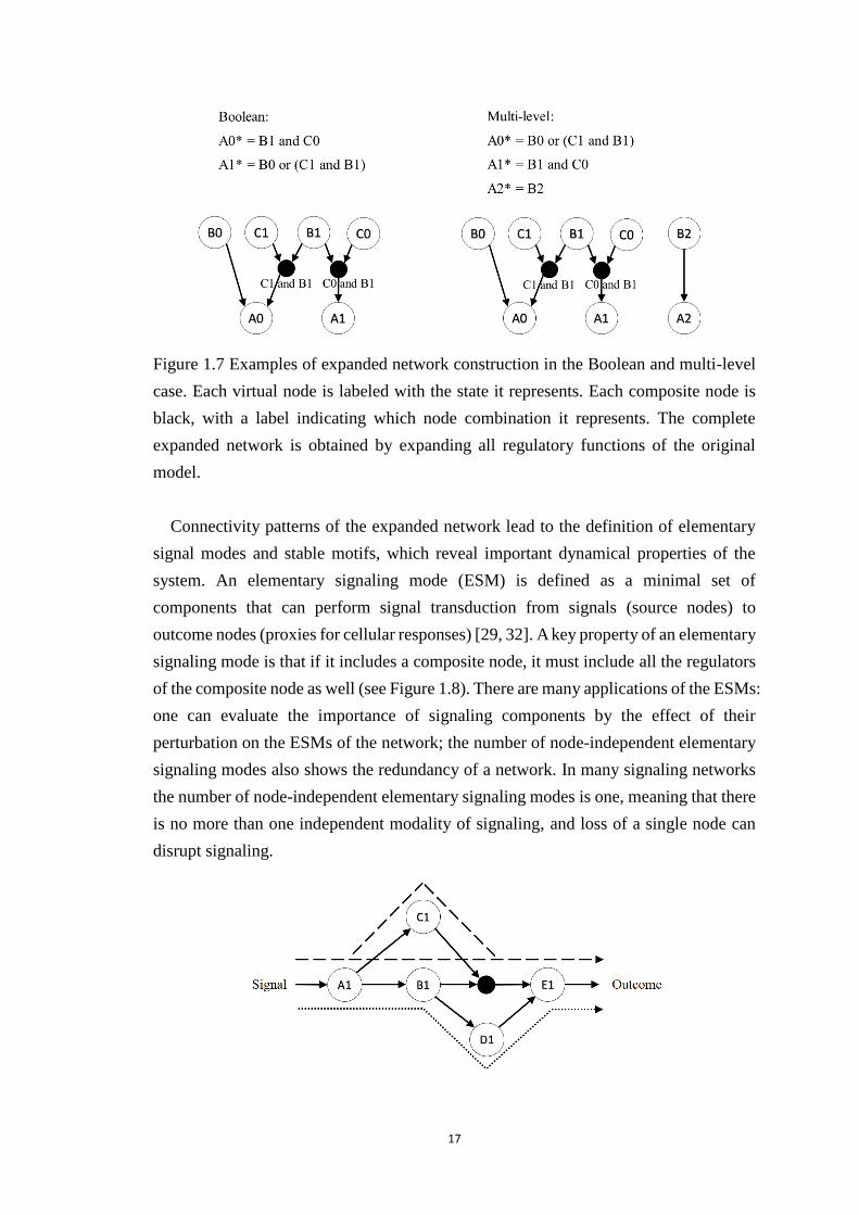
17

Figure 1.7 Examples of expanded network construction in the Boolean and multi-level

case. Each virtual node is labeled with the state it represents. Each composite node is

black, with a label indicating which node combination it represents. The complete

expanded network is obtained by expanding all regulatory functions of the original

model.

Connectivity patterns of the expanded network lead to the definition of elementary

signal modes and stable motifs, which reveal important dynamical properties of the

system. An elementary signaling mode (ESM) is defined as a minimal set of

components that can perform signal transduction from signals (source nodes) to

outcome nodes (proxies for cellular responses) [29, 32]. A key property of an elementary

signaling mode is that if it includes a composite node, it must include all the regulators

of the composite node as well (see Figure 1.8). There are many applications of the ESMs:

one can evaluate the importance of signaling components by the effect of their

perturbation on the ESMs of the network; the number of node-independent elementary

signaling modes also shows the redundancy of a network. In many signaling networks

the number of node-independent elementary signaling modes is one, meaning that there

is no more than one independent modality of signaling, and loss of a single node can

disrupt signaling.

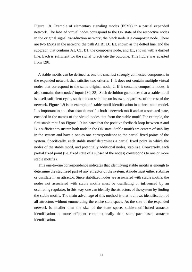
18

Figure 1.8. Example of elementary signaling modes (ESMs) in a partial expanded

network. The labeled virtual nodes correspond to the ON state of the respective nodes

in the original signal transduction network; the black node is a composite node. There

are two ESMs in the network: the path A1 B1 D1 E1, shown as the dotted line, and the

subgraph that contains A1, C1, B1, the composite node, and E1, shown with a dashed

line. Each is sufficient for the signal to activate the outcome. This figure was adapted

from [29].

A stable motifs can be defined as one the smallest strongly connected component in

the expanded network that satisfies two criteria: 1. It does not contain multiple virtual

nodes that correspond to the same original node; 2. If it contains composite nodes, it

also contains these nodes’ inputs [30, 33]. Such definition guarantees that a stable motif

is a self-sufficient cycle, so that it can stabilize on its own, regardless of the rest of the

network. Figure 1.9 is an example of stable motif identification in a three-node model.

It is important to note that a stable motif is both a network motif and an associated state,

encoded in the names of the virtual nodes that form the stable motif. For example, the

first stable motif on Figure 1.9 indicates that the positive feedback loop between A and

B is sufficient to sustain both node in the ON state. Stable motifs are centers of stability

in the system and have a one-to one correspondence to the partial fixed points of the

system. Specifically, each stable motif determines a partial fixed point in which the

nodes of the stable motif, and potentially additional nodes, stabilize. Conversely, each

partial fixed point (i.e. fixed state of a subset of the nodes) corresponds to one or more

stable motif(s).

This one-to-one correspondence indicates that identifying stable motifs is enough to

determine the stabilized part of any attractor of the system. A node must either stabilize

or oscillate in an attractor. Since stabilized nodes are associated with stable motifs, the

nodes not associated with stable motifs must be oscillating or influenced by an

oscillating regulator. In this way, one can identify the attractors of the system by finding

the stable motifs. The main advantage of this method is that it allows identification of

all attractors without enumerating the entire state space. As the size of the expanded

network is smaller than the size of the state space, stable-motif-based attractor

identification is more efficient computationally than state-space-based attractor

identification.

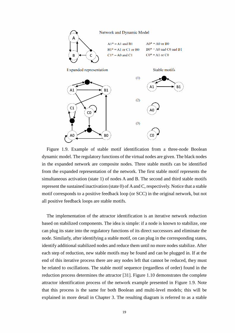
19

Figure 1.9. Example of stable motif identification from a three-node Boolean

dynamic model. The regulatory functions of the virtual nodes are given. The black nodes

in the expanded network are composite nodes. Three stable motifs can be identified

from the expanded representation of the network. The first stable motif represents the

simultaneous activation (state 1) of nodes A and B. The second and third stable motifs

represent the sustained inactivation (state 0) of A and C, respectively. Notice that a stable

motif corresponds to a positive feedback loop (or SCC) in the original network, but not

all positive feedback loops are stable motifs.

The implementation of the attractor identification is an iterative network reduction

based on stabilized components. The idea is simple: if a node is known to stabilize, one

can plug its state into the regulatory functions of its direct successors and eliminate the

node. Similarly, after identifying a stable motif, on can plug in the corresponding states,

identify additional stabilized nodes and reduce them until no more nodes stabilize. After

each step of reduction, new stable motifs may be found and can be plugged in. If at the

end of this iterative process there are any nodes left that cannot be reduced, they must

be related to oscillations. The stable motif sequence (regardless of order) found in the

reduction process determines the attractor [31]. Figure 1.10 demonstrates the complete

attractor identification process of the network example presented in Figure 1.9. Note

that this process is the same for both Boolean and multi-level models; this will be

explained in more detail in Chapter 3. The resulting diagram is referred to as a stable

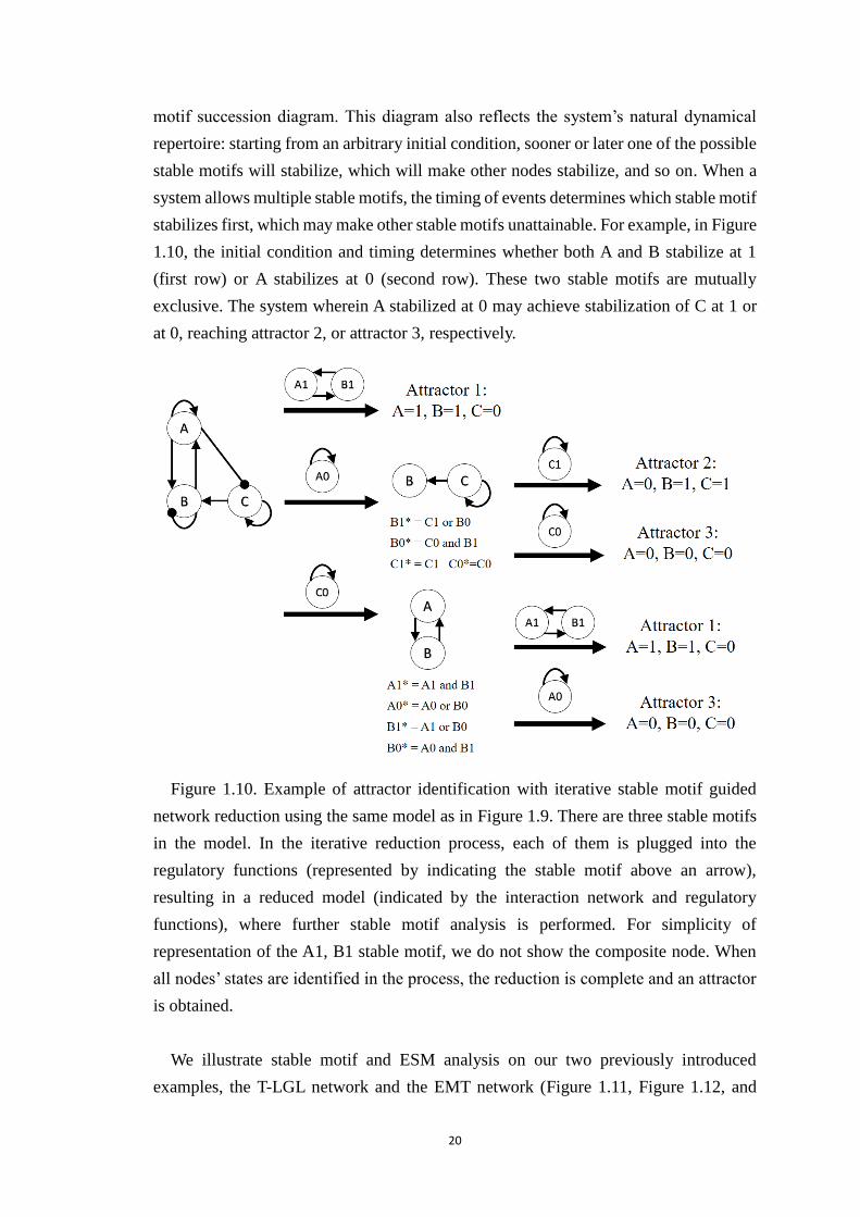
20

motif succession diagram. This diagram also reflects the system’s natural dynamical

repertoire: starting from an arbitrary initial condition, sooner or later one of the possible

stable motifs will stabilize, which will make other nodes stabilize, and so on. When a

system allows multiple stable motifs, the timing of events determines which stable motif

stabilizes first, which may make other stable motifs unattainable. For example, in Figure

1.10, the initial condition and timing determines whether both A and B stabilize at 1

(first row) or A stabilizes at 0 (second row). These two stable motifs are mutually

exclusive. The system wherein A stabilized at 0 may achieve stabilization of C at 1 or

at 0, reaching attractor 2, or attractor 3, respectively.

Figure 1.10. Example of attractor identification with iterative stable motif guided

network reduction using the same model as in Figure 1.9. There are three stable motifs

in the model. In the iterative reduction process, each of them is plugged into the

regulatory functions (represented by indicating the stable motif above an arrow),

resulting in a reduced model (indicated by the interaction network and regulatory

functions), where further stable motif analysis is performed. For simplicity of

representation of the A1, B1 stable motif, we do not show the composite node. When

all nodes’ states are identified in the process, the reduction is complete and an attractor

is obtained.

We illustrate stable motif and ESM analysis on our two previously introduced

examples, the T-LGL network and the EMT network (Figure 1.11, Figure 1.12, and

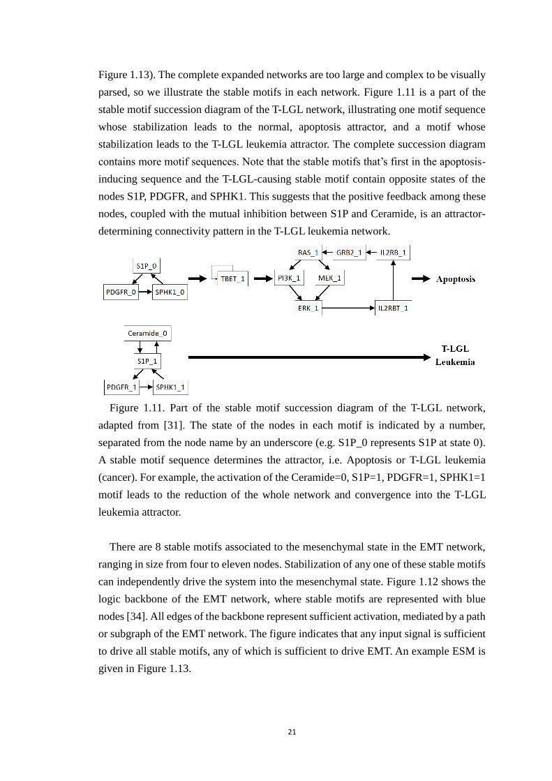
21

Figure 1.13). The complete expanded networks are too large and complex to be visually

parsed, so we illustrate the stable motifs in each network. Figure 1.11 is a part of the

stable motif succession diagram of the T-LGL network, illustrating one motif sequence

whose stabilization leads to the normal, apoptosis attractor, and a motif whose

stabilization leads to the T-LGL leukemia attractor. The complete succession diagram

contains more motif sequences. Note that the stable motifs that’s first in the apoptosis-

inducing sequence and the T-LGL-causing stable motif contain opposite states of the

nodes S1P, PDGFR, and SPHK1. This suggests that the positive feedback among these

nodes, coupled with the mutual inhibition between S1P and Ceramide, is an attractor-

determining connectivity pattern in the T-LGL leukemia network.

Figure 1.11. Part of the stable motif succession diagram of the T-LGL network,

adapted from [31]. The state of the nodes in each motif is indicated by a number,

separated from the node name by an underscore (e.g. S1P_0 represents S1P at state 0).

A stable motif sequence determines the attractor, i.e. Apoptosis or T-LGL leukemia

(cancer). For example, the activation of the Ceramide=0, S1P=1, PDGFR=1, SPHK1=1

motif leads to the reduction of the whole network and convergence into the T-LGL

leukemia attractor.

There are 8 stable motifs associated to the mesenchymal state in the EMT network,

ranging in size from four to eleven nodes. Stabilization of any one of these stable motifs

can independently drive the system into the mesenchymal state. Figure 1.12 shows the

logic backbone of the EMT network, where stable motifs are represented with blue

nodes [34]. All edges of the backbone represent sufficient activation, mediated by a path

or subgraph of the EMT network. The figure indicates that any input signal is sufficient

to drive all stable motifs, any of which is sufficient to drive EMT. An example ESM is

given in Figure 1.13.

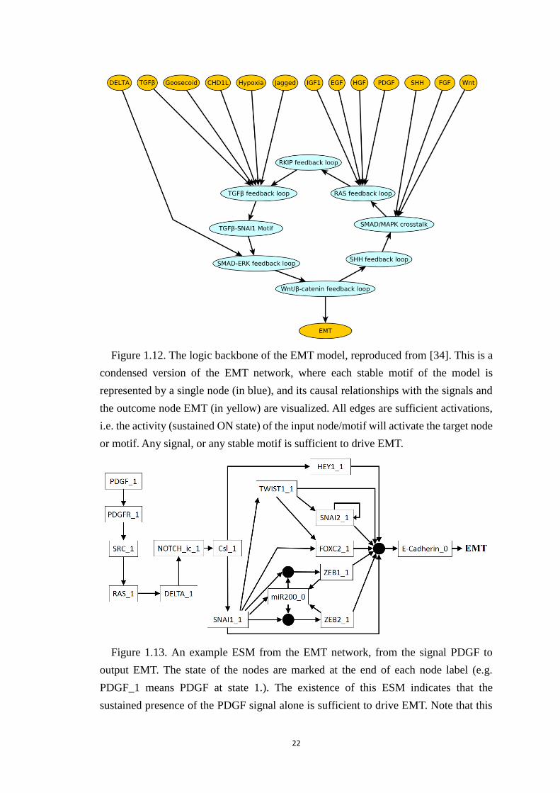
22

Figure 1.12. The logic backbone of the EMT model, reproduced from [34]. This is a

condensed version of the EMT network, where each stable motif of the model is

represented by a single node (in blue), and its causal relationships with the signals and

the outcome node EMT (in yellow) are visualized. All edges are sufficient activations,

i.e. the activity (sustained ON state) of the input node/motif will activate the target node

or motif. Any signal, or any stable motif is sufficient to drive EMT.

Figure 1.13. An example ESM from the EMT network, from the signal PDGF to

output EMT. The state of the nodes are marked at the end of each node label (e.g.

PDGF_1 means PDGF at state 1.). The existence of this ESM indicates that the

sustained presence of the PDGF signal alone is sufficient to drive EMT. Note that this

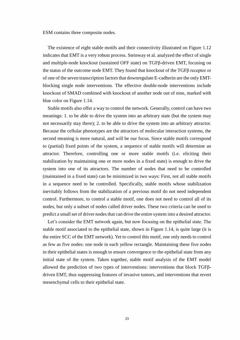
23

ESM contains three composite nodes.

The existence of eight stable motifs and their connectivity illustrated on Figure 1.12

indicates that EMT is a very robust process. Steinway et al. analyzed the effect of single

and multiple-node knockout (sustained OFF state) on TGFβ-driven EMT, focusing on

the status of the outcome node EMT. They found that knockout of the TGFβ receptor or

of one of the seven transcription factors that downregulate E-cadherin are the only EMT-

blocking single node interventions. The effective double-node interventions include

knockout of SMAD combined with knockout of another node out of nine, marked with

blue color on Figure 1.14.

Stable motifs also offer a way to control the network. Generally, control can have two

meanings: 1. to be able to drive the system into an arbitrary state (but the system may

not necessarily stay there); 2. to be able to drive the system into an arbitrary attractor.

Because the cellular phenotypes are the attractors of molecular interaction systems, the

second meaning is more natural, and will be our focus. Since stable motifs correspond

to (partial) fixed points of the system, a sequence of stable motifs will determine an

attractor. Therefore, controlling one or more stable motifs (i.e. eliciting their

stabilization by maintaining one or more nodes in a fixed state) is enough to drive the

system into one of its attractors. The number of nodes that need to be controlled

(maintained in a fixed state) can be minimized in two ways: First, not all stable motifs

in a sequence need to be controlled. Specifically, stable motifs whose stabilization

inevitably follows from the stabilization of a previous motif do not need independent

control. Furthermore, to control a stable motif, one does not need to control all of its

nodes, but only a subset of nodes called driver nodes. These two criteria can be used to

predict a small set of driver nodes that can drive the entire system into a desired attractor.

Let’s consider the EMT network again, but now focusing on the epithelial state. The

stable motif associated to the epithelial state, shown in Figure 1.14, is quite large (it is

the entire SCC of the EMT network). Yet to control this motif, one only needs to control

as few as five nodes: one node in each yellow rectangle. Maintaining these five nodes

in their epithelial states is enough to ensure convergence to the epithelial state from any

initial state of the system. Taken together, stable motif analysis of the EMT model

allowed the prediction of two types of interventions: interventions that block TGFβ-

driven EMT, thus suppressing features of invasive tumors, and interventions that revert

mesenchymal cells to their epithelial state.

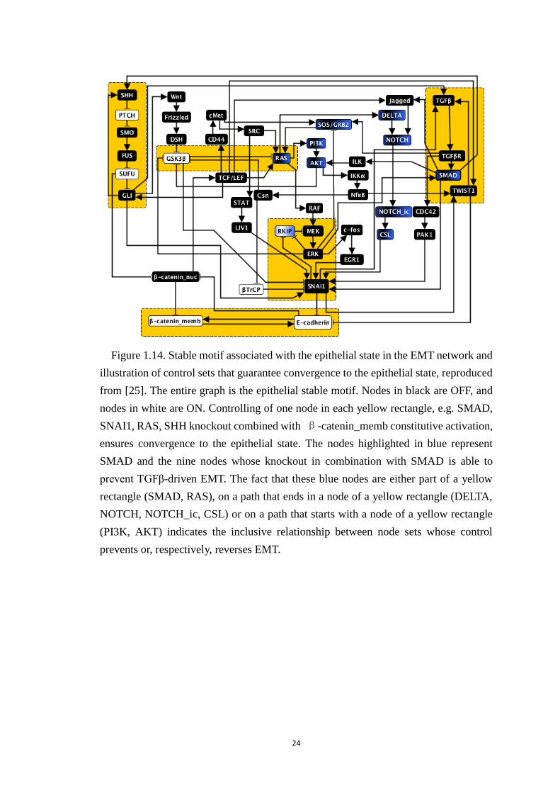
24

Figure 1.14. Stable motif associated with the epithelial state in the EMT network and

illustration of control sets that guarantee convergence to the epithelial state, reproduced

from [25]. The entire graph is the epithelial stable motif. Nodes in black are OFF, and

nodes in white are ON. Controlling of one node in each yellow rectangle, e.g. SMAD,

SNAI1, RAS, SHH knockout combined with β-catenin_memb constitutive activation,

ensures convergence to the epithelial state. The nodes highlighted in blue represent

SMAD and the nine nodes whose knockout in combination with SMAD is able to

prevent TGFβ-driven EMT. The fact that these blue nodes are either part of a yellow

rectangle (SMAD, RAS), on a path that ends in a node of a yellow rectangle (DELTA,

NOTCH, NOTCH_ic, CSL) or on a path that starts with a node of a yellow rectangle

(PI3K, AKT) indicates the inclusive relationship between node sets whose control

prevents or, respectively, reverses EMT.

25

Chapter 2 Analysis of a dynamic model of guard cell

signaling reveals the stability of signal propagation

Most of this chapter is based on previously published work for which I am the first

author [2]. Parts of the published work are reproduced in this chapter from BMC

Systems Biology (open access).

Background

Modeling offers a comprehensive way to understand biological processes by

integrating the components involved in them and the interactions between components.

Models can recapitulate and explain the emergent outcome(s) of the process [35, 36].

Representing cellular processes that involve many proteins and small molecules by a

signal transduction network can reveal indirect relationships between components and

provide new insight [37-39]. Such network usually consists of nodes representing

biological entities, and edges representing interactions. Once a network has been

constructed, dynamic modeling, where each node in the network is associated with a

variable representing its abundance or activity, can further describe the behavior of the

network. Dynamic models can have continuous variables whose change is described by

differential equations [40], discrete variables described by discrete (logical) regulatory

functions [3, 41], or a combination of continuous and discrete variables [42]. The major

advantage of discrete dynamic and continuous-discrete hybrid modeling is that they use

much fewer parameters than continuous models and thus need less parameter estimation

[11, 18, 43]. Modeling allows one to analyze the biological system represented by the

network in silico, when performing the relevant experiment is infeasible. It also helps

identify general principles of biological systems [44, 45].

The biological process of stomatal opening in plants is a good example of a complex

system wherein modeling leads to significant gain in understanding [1, 46]. Stomata are

pores on leaf surfaces that allow the plant to exchange carbon dioxide (CO2) and oxygen

with the atmosphere. Stomata are formed by two guard cells that can change shape:

swelling of guard cells leads to stomatal opening; their shrinking leads to stomatal

closure. The shape of each guard cell is directly controlled by water flow through the

membrane, which is in turn controlled by ion flow. Different signals can affect the guard

cell, changing its ion concentration in direct and indirect ways, resulting in stomatal

opening or closure [47-49]. These signals include light of different wavelengths, CO2

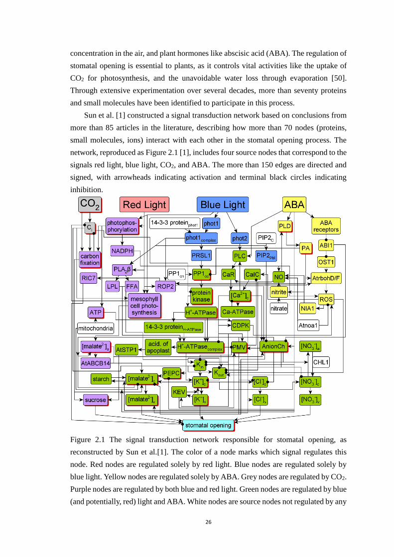
26

concentration in the air, and plant hormones like abscisic acid (ABA). The regulation of

stomatal opening is essential to plants, as it controls vital activities like the uptake of

CO2 for photosynthesis, and the unavoidable water loss through evaporation [50].

Through extensive experimentation over several decades, more than seventy proteins

and small molecules have been identified to participate in this process.

Sun et al. [1] constructed a signal transduction network based on conclusions from

more than 85 articles in the literature, describing how more than 70 nodes (proteins,

small molecules, ions) interact with each other in the stomatal opening process. The

network, reproduced as Figure 2.1 [1], includes four source nodes that correspond to the

signals red light, blue light, CO2, and ABA. The more than 150 edges are directed and

signed, with arrowheads indicating activation and terminal black circles indicating

inhibition.

Figure 2.1 The signal transduction network responsible for stomatal opening, as

reconstructed by Sun et al.[1]. The color of a node marks which signal regulates this

node. Red nodes are regulated solely by red light. Blue nodes are regulated solely by

blue light. Yellow nodes are regulated solely by ABA. Grey nodes are regulated by CO2.

Purple nodes are regulated by both blue and red light. Green nodes are regulated by blue

(and potentially, red) light and ABA. White nodes are source nodes not regulated by any

27

of the four signals. To improve visualization, certain pairs of edges with the same

starting or end nodes overlap. Nodes with multiple levels in the dynamic model are

represented by red shadows; the others are Boolean. The full names of the network

components denoted by abbreviated node names are given in Table 1. This figure and

part of its caption is reproduced from Sun Z, Jin X, Albert R, Assmann SM (2014)

Multi-level Modeling of Light-Induced Stomatal Opening Offers New Insights into Its

Regulation by Drought. PLoS Comput Biol 10(11): e1003930.

doi:10.1371/journal.pcbi.1003930.

Translating this network into a dynamic model, Sun et al. characterized each node

with a discrete variable describing its activity and with a discrete (logical) regulatory

function describing its regulation. Twenty-one out of the 70 nodes in the model are

multi-level, the rest are Boolean (binary). The levels reflect relative and qualitative

information: a level of 2 is a higher level than 1, but should not be interpreted as twice

as high. A few discrete values are not integers; e.g. stomatal opening is a weighted sum

with non-integer weights. The dynamic model has ~1031 states. The logical regulatory

functions, describing each node’s future state based on the states of the node’s regulators,

use a combination of Boolean logic operators (And, Or, Not), algebraic operations, and

input-output tables. For example, the regulatory function of PRSL1 is:

PRSL1* = phot1complex Or phot2.

Here for simplicity the node states are denoted by the node names; the asterisk in

“PRSL1*” indicates that this will be the next state of the PRSL1. The “Or” Boolean

operator expresses that either of the blue light receptors, i.e. the phot1 complex or phot2,

can independently activate PRSL1.

The Sun et al. model starts from an initial condition representative of closed stomata.

Then a combination of the four input signals is applied. Red light, blue light, and ABA

are represented as binary variables, and external CO2 is represented with three states: 0

(CO2 free air), 1 (ambient CO2) and 2 (high CO2). The system’s response is simulated

through repetitive re-evaluation of each node’s state until a stable value of stomatal

opening is observed. The model successfully captured stomatal opening in response to

combinations of the signals. It also successfully reproduces stomatal opening under

most of the experimentally studied perturbation scenarios (i.e. genetic knockouts or

external supply of components). In total, the model is consistent with 63 out of 66

experimental observations collected by Sun et al. [1]. The model predicts the outcome

of a large number of scenarios that have not been explored experimentally so far. It also

revealed a gap of knowledge regarding the cross-talk of red light and ABA signaling,

28

and filled it with a newly predicted interaction.

Although the Sun et al. model recapitulates existing knowledge and offers new

predictions, the model's full dynamic repertoire could not be characterized due to its

large state space. Instead, Sun et al. focused on tracking the output node, stomatal

opening, and a few selected internal nodes, in time. In this chapter we apply multiple

methods to analyze the model and aim to fully map all its potential long-term behaviors,

or in other words, attractors.

Methods

Attractors of a dynamical system

An attractor is a set of states from which only states in the same set can be reached.

Attractors that consist of a single state are called stable steady states or fixed points;

attractors that contain multiple states are called complex attractors or oscillations [11].

In biological networks, attractors often have significant biological meaning. In a cell

signaling network, attractors correspond to cell types, cell fates or behaviors [51]. For

example, one attractor can represent a healthy differentiated cell, while another attractor

can represent an abnormally motile cancer cell [24].

Update scheme of a discrete time model

In the Sun et al. model, as in most discrete dynamic models, time is an implicit

variable. As there is very little information about the kinetics of the nodes in the stomatal

opening network, the model incorporates an element of stochasticity in timing. The

timing does not affect a system’s fixed point attractors, but it can change the complex

attractors and the possibility of reaching a given attractor from a given initial state [11].

In the Sun et al. model, a random–order asynchronous update is used. Specifically, at

each time step, a random order of nodes (excluding the four input nodes and the output

node stomatal opening) is generated, and each node’s state is reevaluated in this order;

stomatal opening is always updated last. In the next time step a different order is selected

randomly. In this chapter, we use a different type of stochastic update, called general

asynchronous update, wherein a randomly selected node is updated at each time step.

This is required by the network reduction method we use. Although this theoretically

could cause a difference in complex attractors, we will show that in this specific model

the two methods yield the same attractors.

Network reduction

To reduce the Sun et al. model’s state space, we apply a network reduction method

developed by Saadatpour et al. [13] that is proven to preserve the attractors in a Boolean

model. Two types of nodes can be reduced (eliminated or merged): source nodes with

29

no incoming edges, and simple mediator nodes that have one incoming and/or one

outgoing edge. In the reduction, the source node’s state is directly plugged into the

regulatory function of all of its direct successor nodes; then the source node is

eliminated. For a simple mediator node with one predecessor (regulator) and one

successor (target), its regulator is connected to its target and the mediator node is merged

into the regulator. If there is one regulator and several targets of the mediator node, but

no direct edges between the regulator and any of the targets, the mediator node is merged

into the regulator. Conversely, if there are several regulators and one target of the

mediator node, but no direct edges among any of the regulators and the target, the

mediator node is merged into its target. Although this method is not proven in the multi-

level case, we conjecture that attractors are also conserved for a multi-level mode, and

will show from the results that in the Sun et al. model this reduction method preserved

all attractors.

Elimination of redundant edges

During the process of creating a discrete dynamic model from biological data, when

an influence is weaker than other influences, the modeler may choose to omit this

influence or, alternatively, include it a redundant way. The latter choice was made by

Sun et al. in four cases, leading to four regulatory functions that contain an input that

does not affect the outcome of the regulatory function. One of these is

ROS* = NADPH And AtrbohD/F Or NADPH And AtrbohD/F And CDPK Or Not

Atnoa1

The italicized words “And”, “Or” and “Not” are Boolean logic operators; the non-

italicized words represent node names. In this regulatory function every node is Boolean

(binary). The first clause “NADPH And AtrbohD/F” and the second “NADPH And

AtrbohD/F And CDPK” are connected with an “Or” rule, with the result that the node

“CDPK” does not have any influence on the outcome. Therefore, we can reduce the

edge from CDPK to ROS without changing the model’s dynamics. We similarly prune

three additional redundant edges.

Converting a multi-level model to Boolean

There are several possibilities to convert a multi-level model to Boolean [52]. The

standard method used in the case of logical models of regulatory networks is the Van

Ham mapping [53, 54]. It preserves the dynamics of the original model if the variables

in the original model can be represented by integers and if the original model only

allows state transitions in which one node changes its state by one level [54]. The Sun

et al. model does not satisfy these criteria. However there still is a conclusion that we

can use: All types of conversions maintain the fixed points and the reachability of states

(i.e. if there is a sequence of state transitions from state A to state B before conversion,

30

there must be a sequence of state transitions from the corresponding state A’ to state

B’ after the conversion) [54]. So the worst distortion of attractors due to the conversion

is the merging of two complex attractors into one. In this light we choose to use an

economic mapping of each multi-level node into as many Boolean nodes as necessary

for the binary representation of the corresponding integer. We will show that in this

specific model, the conversion did not change the attractors.

Results

Network reduction

The Sun et al. model has a huge state space of ~1031 states, making its analysis

difficult. To obtain a smaller state space, we reduce the size of the network by applying

a network reduction technique developed by Saadatpour et al. [13] that is proven to

preserve the attractors of Boolean models (see Methods). All source nodes other than

the four signals (blue light, red light, CO2, and abscisic acid) and all simple mediator

nodes are identified and reduced. This process is done iteratively until it cannot be done

any more. A total of 7 source nodes (14-3-3 proteinphot1, PIP2C, AtNOA1, Nitrate, PP1cn,

mitochondria, and CHL1), and 19 simple mediator nodes (phot1, phot2, NIA1, H+-

ATPase, LPL, ATP, acid. of apoplast, [NO3-]v, [Cl-]v, NADPH, [malate2-]v, PA, ABA

receptors, OST1, PRSL1, PIP2PM, AtrbohD/F, Nitrite, and phot1complex) are eliminated.

Several of the simple mediator nodes form linear paths (e.g. phot1, OST1) thus their

iterative reduction shortens the linear paths in the network. In addition, 16 of the 19

reduced mediators have a regulatory function of the form “B* =A”. It is intuitive that

reduction of this node type preserves the attractors.

We do not eliminate the four signal nodes because we want to simultaneously

explore all the combinations of input signals. We also choose to not reduce the five

nodes (Kin, Kout, Kc, Ca2+-ATPase, mesophyll cell photosynthesis) whose merging with

their sole regulator would result in a self-loop (self-regulation), because such self-loops

may be difficult to interpret. Two additional nodes with significant biological meaning

to the network (sucrose, stomatal opening), are not reduced either.

Another form of network reduction is the elimination of redundant edges (see

Methods). After removal of redundant edges, the node CDPK becomes a sink node, thus

it can also be eliminated. The reduction of the above-described nodes and redundant

edges simplifies the network from 70 nodes to 42 nodes, with an estimated state space

of ~1022 states.

Simplification of regulatory functions

In order to further reduce the state space from ~1022 to a manageable size, we

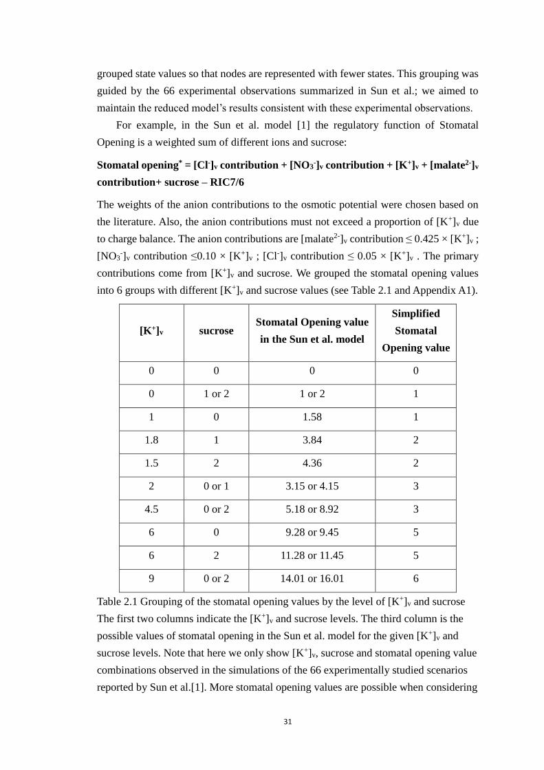
31

grouped state values so that nodes are represented with fewer states. This grouping was

guided by the 66 experimental observations summarized in Sun et al.; we aimed to

maintain the reduced model’s results consistent with these experimental observations.

For example, in the Sun et al. model [1] the regulatory function of Stomatal

Opening is a weighted sum of different ions and sucrose:

Stomatal opening* = [Cl-]v contribution + [NO3-]v contribution + [K+]v + [malate2-]v

contribution+ sucrose – RIC7/6

The weights of the anion contributions to the osmotic potential were chosen based on

the literature. Also, the anion contributions must not exceed a proportion of [K+]v due

to charge balance. The anion contributions are [malate2-]v contribution ≤ 0.425 × [K+]v ;

[NO3-]v contribution ≤0.10 × [K+]v ; [Cl-]v contribution ≤ 0.05 × [K+]v . The primary

contributions come from [K+]v and sucrose. We grouped the stomatal opening values

into 6 groups with different [K+]v and sucrose values (see Table 2.1 and Appendix A1).

[K+]v sucrose Stomatal Opening value

in the Sun et al. model

Simplified

Stomatal

Opening value

0 0 0 0

0 1 or 2 1 or 2 1

1 0 1.58 1

1.8 1 3.84 2

1.5 2 4.36 2

2 0 or 1 3.15 or 4.15 3

4.5 0 or 2 5.18 or 8.92 3

6 0 9.28 or 9.45 5

6 2 11.28 or 11.45 5

9 0 or 2 14.01 or 16.01 6

Table 2.1 Grouping of the stomatal opening values by the level of [K+]v and sucrose

The first two columns indicate the [K+]v and sucrose levels. The third column is the

possible values of stomatal opening in the Sun et al. model for the given [K+]v and

sucrose levels. Note that here we only show [K+]v, sucrose and stomatal opening value

combinations observed in the simulations of the 66 experimentally studied scenarios

reported by Sun et al.[1]. More stomatal opening values are possible when considering

32

node perturbations. The 4th column shows the simplified stomatal opening level after

grouping. The update function for the simplified stomatal opening level covers all

possible values of [K+]v and sucrose (see Appendix A1).

Similarly to the original model, the simplified states represent qualitative, relative

categories. For example, a stomatal opening level of 2 is not twice as high as level 1.

We choose the simplified stomatal opening values so that there is no state “4”, to better

reflect an experimentally observed synergistic effect between blue and red light [48, 49,

55]. Simulation results with the simplified regulatory function are that under

monochromatic red light stomatal opening =1; under monochromatic blue light stomatal

opening =3; under dual beam the stomatal opening =5, which is larger than the sum

“1+3”. This qualitatively reproduces the experimental observation that under dual beam

illumination stomata open to a size much larger than the sum of opening under

monochromatic blue or red light.

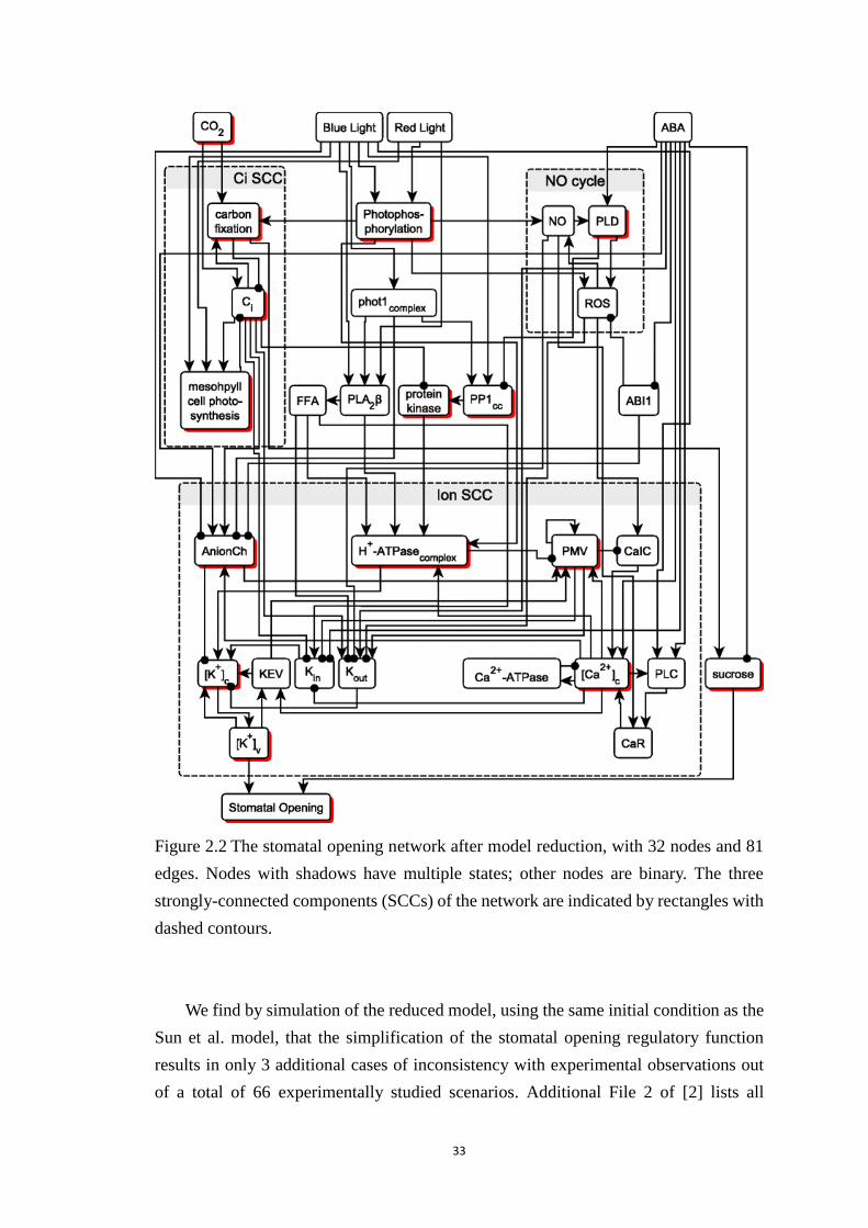
33

Figure 2.2 The stomatal opening network after model reduction, with 32 nodes and 81

edges. Nodes with shadows have multiple states; other nodes are binary. The three

strongly-connected components (SCCs) of the network are indicated by rectangles with

dashed contours.

We find by simulation of the reduced model, using the same initial condition as the

Sun et al. model, that the simplification of the stomatal opening regulatory function

results in only 3 additional cases of inconsistency with experimental observations out

of a total of 66 experimentally studied scenarios. Additional File 2 of [2] lists all

34

experimental observations and compares them to the relevant simulation results.

Ignoring the contribution of malate2- , NO3-, and RIC7 to stomatal opening each causes

one additional discrepancy; ignoring Cl- does not cause any additional discrepancy.

Ignoring these nodes trades a decrease in accuracy for a significant increase in simplicity.

The simplification of the stomatal opening regulatory function eliminates the effect

of vacuolar anions and of RIC7 on stomatal opening. As a result we can further simplify

the Sun et al. model by eliminating 10 nodes in total, [malate2-]a, [malate2-]c, starch,

[Cl-]c, [NO3-]c, [NO3

-]a, ROP2, RIC7, ABC, and PEPC. The only edge from these nodes

to other nodes is [malate2-]a → AnionCh. In section 3, Additional File 3 of [2] we show

that eliminating this edge does not change the system’s long-term behavior, i.e.

attractors. Also, the regulatory function describing the cytosolic K+ concentration, [K+]c,

can be simplified without loss, as described in section 3, Additional File 3 of [2]. After

this simplification we have a network of 32 nodes, 81 edges, indicated on Figure 2.2.

We will refer to this model as the “reduced model”. A list of nodes and their regulatory

functions is provided in Appendix A1.

Identifying strongly connected components (SCCs) is important for attractor

analysis, as complex dynamic behavior such as oscillations or multi-stability requires

feedback loops [3]. There are three SCCs in the network of the reduced model, as

marked in Figure 2.2. The NO cycle contains three nodes and three positive edges. The

Ci SCC contains three nodes, which form two negative feedback loops. The Ion SCC is

the most complex, containing 13 nodes and 26 edges, 7 of which are negative.

Next we perform attractor analysis using two methods: 1. by converting the reduced

model to Boolean and applying two analysis tools; 2. by analyzing the regulatory

functions theoretically. The former method finds all stable steady states and candidate

oscillations; the latter confirms the results of the first method and gives insight about

perturbation scenarios.

Conversion of nodes from multi-level to Boolean states and attractor analysis

We perform the conversion to Boolean to enable attractor analysis by existing

software tools. Zañudo et al. [30] proposed an algorithm to find the attractors of a

Boolean network based on the concept of “stable motif”, a strongly-connected group of

nodes that can stabilize regardless of their inputs. The algorithm finds all stable motifs,

which determine the part of the network that stabilizes in an attractor. After a stable

motif is found, one can plug in its stabilized state into the network, and obtain a smaller

remaining network. After repeating this, eventually the remaining part is either nothing

(indicating a fixed point/steady state) or a candidate oscillating sub-network. Compared

with other software tools [16, 56], the major advantage of this algorithm is that it finds

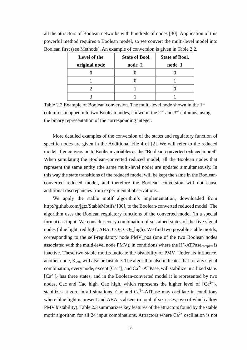
35

all the attractors of Boolean networks with hundreds of nodes [30]. Application of this

powerful method requires a Boolean model, so we convert the multi-level model into

Boolean first (see Methods). An example of conversion is given in Table 2.2.

Level of the

original node

State of Bool.

node_2

State of Bool.

node_1

0 0 0

1 0 1

2 1 0

3 1 1

Table 2.2 Example of Boolean conversion. The multi-level node shown in the 1st

column is mapped into two Boolean nodes, shown in the 2nd and 3rd columns, using

the binary representation of the corresponding integer.

More detailed examples of the conversion of the states and regulatory function of

specific nodes are given in the Additional File 4 of [2]. We will refer to the reduced

model after conversion to Boolean variables as the “Boolean-converted reduced model”.

When simulating the Boolean-converted reduced model, all the Boolean nodes that

represent the same entity (the same multi-level node) are updated simultaneously. In

this way the state transitions of the reduced model will be kept the same in the Boolean-

converted reduced model, and therefore the Boolean conversion will not cause

additional discrepancies from experimental observations.

We apply the stable motif algorithm’s implementation, downloaded from

http://github.com/jgtz/StableMotifs/ [30], to the Boolean-converted reduced model. The

algorithm uses the Boolean regulatory functions of the converted model (in a special

format) as input. We consider every combination of sustained states of the five signal

nodes (blue light, red light, ABA, CO2, CO2_high). We find two possible stable motifs,

corresponding to the self-regulatory node PMV_pos (one of the two Boolean nodes

associated with the multi-level node PMV), in conditions where the H+-ATPasecomplex is

inactive. These two stable motifs indicate the bistability of PMV. Under its influence,

another node, Kout, will also be bistable. The algorithm also indicates that for any signal

combination, every node, except [Ca2+]c and Ca2+-ATPase, will stabilize in a fixed state.

[Ca2+]c has three states, and in the Boolean-converted model it is represented by two

nodes, Cac and Cac_high. Cac_high, which represents the higher level of [Ca2+]c,

stabilizes at zero in all situations. Cac and Ca2+-ATPase may oscillate in conditions

where blue light is present and ABA is absent (a total of six cases, two of which allow

PMV bistability). Table 2.3 summarizes key features of the attractors found by the stable

motif algorithm for all 24 input combinations. Attractors where Ca2+ oscillation is not

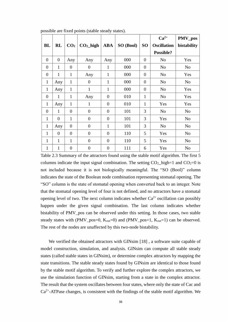
36

possible are fixed points (stable steady states).

BL RL CO2 CO2_high ABA SO (Bool) SO

Ca2+

Oscillation

Possible?

PMV_pos

bistability

0 0 Any Any Any 000 0 No Yes

0 1 0 0 1 000 0 No No

0 1 1 Any 1 000 0 No Yes

1 Any 1 0 1 000 0 No No

1 Any 1 1 1 000 0 No Yes

0 1 1 Any 0 010 1 No Yes

1 Any 1 1 0 010 1 Yes Yes

0 1 0 0 0 101 3 No No

1 0 1 0 0 101 3 Yes No

1 Any 0 0 1 101 3 No No

1 0 0 0 0 110 5 Yes No

1 1 1 0 0 110 5 Yes No

1 1 0 0 0 111 6 Yes No

Table 2.3 Summary of the attractors found using the stable motif algorithm. The first 5

columns indicate the input signal combination. The setting CO2_high=1 and CO2=0 is

not included because it is not biologically meaningful. The “SO (Bool)” column

indicates the state of the Boolean node combination representing stomatal opening. The

“SO” column is the state of stomatal opening when converted back to an integer. Note

that the stomatal opening level of four is not defined, and no attractors have a stomatal

opening level of two. The next column indicates whether Ca2+ oscillation can possibly

happen under the given signal combination. The last column indicates whether

bistability of PMV_pos can be observed under this setting. In those cases, two stable

steady states with (PMV_pos=0, Kout=0) and (PMV_pos=1, Kout=1) can be observed.

The rest of the nodes are unaffected by this two-node bistability.

We verified the obtained attractors with GINsim [18] , a software suite capable of

model construction, simulation, and analysis. GINsim can compute all stable steady

states (called stable states in GINsim), or determine complex attractors by mapping the

state transitions. The stable steady states found by GINsim are identical to those found

by the stable motif algorithm. To verify and further explore the complex attractors, we

use the simulation function of GINsim, starting from a state in the complex attractor.

The result that the system oscillates between four states, where only the state of Cac and

Ca2+-ATPase changes, is consistent with the findings of the stable motif algorithm. We

37

provide the summary of GINsim computation/simulation results in Additional File 7 of

[2]. Additional File 8 of [2] indicates the Boolean-converted reduced model in SBML-

qual format [16], a general format for biological model to be analyzed using various

tools including GINsim.

We can also connect the stable motif analysis results to network reduction. We have

previously decided to not reduce the four nodes that correspond to input signals. If we

do consider a specific input combination when using network reduction, e.g. blue light

and red light with normal CO2 without ABA, we can reduce much more of the network:

two of the three SCCs, namely the NO cycle and the Ci SCC, will stabilize and get

reduced. Only the Ion SCC and its sole output stomatal opening remain, indicating that

this SCC is not driven solely by the external signals and has the capacity for oscillations

or multi-stability. This is consistent with the results found by stable motif analysis,

according to which the NO cycle and the Ci SCC attain a steady state and the Ion SCC

admits a [Ca2+]c - Ca2+-ATPase oscillation and PMV bistability. This consistency

supports the appropriateness of the network reduction method and of the Boolean

conversion.”

Theoretical analysis of the reduced model

To gain additional insight into the attractors of the reduced model and their potential

changes due to node perturbations, we analyze the reduced model theoretically.

Specifically, we aim to answer the question: Can there be other types of oscillation, or

can there be additional multi-stability, if a node is knocked out (fixed in the OFF state)

or is constitutive active (fixed in the ON state)?

We first test whether the network and regulatory rules allow multi-stability or

oscillations. This analysis is based on R. Thomas’s conjectures [3]: The presence of a

positive (negative) feedback loop - a cycle with an even (odd) number of inhibitory

edges - in the network is a necessary but not sufficient condition for the occurrence of

multiple steady states (oscillations). The conjectures have been proven in the case of

discrete dynamic systems [26-28, 57]. Since only feedback loops are candidates for

potential multi-stability or oscillations, we analyze the regulatory functions of each

strongly connected component of the network. For each feedback loop, we identify a

sufficient condition for the nodes to stabilize in a specific state. The violation of this

condition becomes a further necessary condition of multi-stability or oscillation. Here

we describe the main steps and results of the analysis; the detailed analysis is in

Additional File 3 of [2].

The NO cycle is composed of the nodes PLD, ROS, NO, and the three positive

edges between them. It does not have any negative edges, so it cannot oscillate. A fixed

38

ABA value is sufficient to stabilize each node of the cycle in a specific state, thus the

cycle does not admit multi-stability under any perturbation.

The Ci SCC has three nodes, Ci, mesophyll cell photosynthesis (MCPS), carbon

fixation, and four edges that form two negative feedback loops, one between carbon

fixation and Ci, and the other between Ci and MCPS. Despite the existence of negative

feedback, this cycle will stabilize if given a fixed CO2 value. From this we know that

this cycle cannot oscillate or admit multi-stability under any perturbation.

The Ion SCC has 13 nodes. To reduce its complexity we show that the key node

[Ca2+]c, which has states 0,1, and 2, cannot enter state 2 in the long term under any

perturbation. Since most nodes respond to [Ca2+]c only if [Ca2+]c =2, we can eliminate

all edges that depend only on “[Ca2+]c =2”, and obtain a simplified Ion SCC, as shown

in Figure 2.3. The Ca2+ SCC ([Ca2+]c, Ca2+ ATPase, PLC, CaR) now becomes a sink

SCC. The only negative edge in this sub-network is from Ca2+-ATPase to [Ca2+]c. These

two nodes are known to oscillate. The positive feedback loop formed by [Ca2+]c, PLC,

and CaR will stabilize if given fixed inputs. So there cannot be multi-stability. For the

nodes outside of the Ca2+ feedback loops, we show that the edges from KEV and [K+]v

are redundant in the long term, so there are no feedback loops except the PMV self-loop.

PMV is not capable of having oscillations, but can have bistability (as also indicated by

the stable motif analysis). The bistability can affect at most one other node, Kout, under

any perturbation. This means that the bistability has very limited effect on the attractor

of the reduced model.

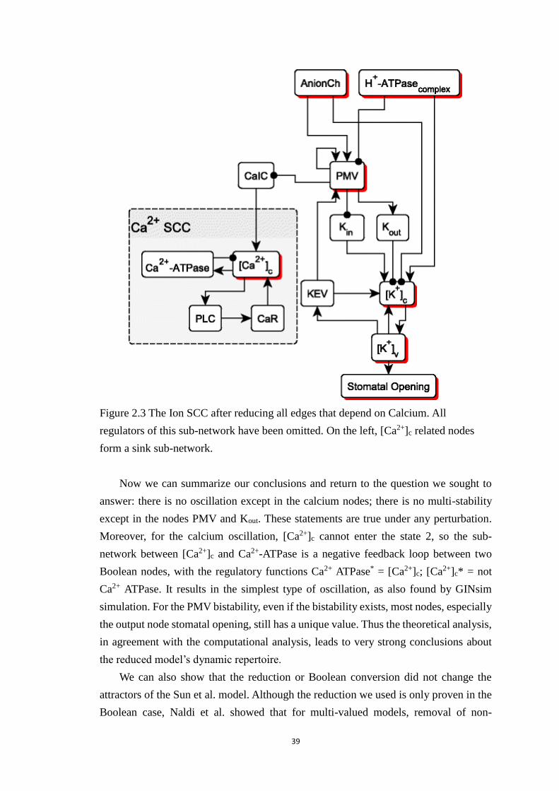
39

Figure 2.3 The Ion SCC after reducing all edges that depend on Calcium. All

regulators of this sub-network have been omitted. On the left, [Ca2+]c related nodes

form a sink sub-network.

Now we can summarize our conclusions and return to the question we sought to

answer: there is no oscillation except in the calcium nodes; there is no multi-stability

except in the nodes PMV and Kout. These statements are true under any perturbation.

Moreover, for the calcium oscillation, [Ca2+]c cannot enter the state 2, so the sub-

network between [Ca2+]c and Ca2+-ATPase is a negative feedback loop between two

Boolean nodes, with the regulatory functions Ca2+ ATPase* = [Ca2+]c; [Ca2+]c* = not

Ca2+ ATPase. It results in the simplest type of oscillation, as also found by GINsim

simulation. For the PMV bistability, even if the bistability exists, most nodes, especially

the output node stomatal opening, still has a unique value. Thus the theoretical analysis,

in agreement with the computational analysis, leads to very strong conclusions about

the reduced model’s dynamic repertoire.

We can also show that the reduction or Boolean conversion did not change the

attractors of the Sun et al. model. Although the reduction we used is only proven in the

Boolean case, Naldi et al. showed that for multi-valued models, removal of non-

40

autoregulated nodes, like in our reduction, preserves crucial dynamical properties [14],

including fixed point attractors and the two-node simple oscillation we found. So our

reduction is valid in this specific model. To confirm that the Boolean conversion

preserved attractors, we note that in the Boolean-converted reduced model we found

fixed point attractors and a complex attractor in which only two nodes oscillate. Because

the only potential change to attractors as a consequence of the conversion is merging of

complex attractors [54], it is straightforward that the attractors have been conserved

during the conversion, as the two-node oscillation found is the simplest type of complex

attractor and cannot be a result of attractor merging. In addition, using general

asynchronous update instead of random order asynchronous update does not cause any

changes to the attractor, because the update schemes do not affect fixed points or the

two-node simple oscillation we found.

Stability of guard cell signal transduction

Our previous results indicate the stability of the system in the sense that all the

initial conditions lead to the same attractor except for up to four nodes. We also examine

another facet of the system’s stability: the robustness of the stomatal opening in response

to node perturbations that render them non-functional. We perform a systematic set of

single-node knockouts of every non-signal node in the reduced model, under all

combinations of light, CO2 and ABA conditions. For each signal combination, we set

the perturbed node’s initial state and regulatory function to 0, initialize the rest of the

nodes in the condition representative of closed stomata, and then simulate the reduced

model until it reaches its attractor. In the absence of ABA under each light and CO2

condition, 60%-90% perturbation scenarios produce the same stomatal opening value

as the unperturbed system (Table 2.4). These results are similar to those reported by Sun

et al. for the original model [1] (Appendix A2). In the presence of ABA 50%-90%

perturbation scenarios produce the same stomatal opening value as the unperturbed

system, and 4-16% knockouts lead to a higher stomatal opening value. Perturbations in

the ABA=1 case were not studied by Sun et al., but our simulations of the original model

give the same qualitative results as the reduced model. These results indicate the

closeness of the perturbed attractor (at least in terms of the stomatal opening value) to

the unperturbed attractor in more than 50% of single node perturbations. They also

suggest the resilience of the stomatal opening process against internal failures and

perturbations.

Light, CO2 and ABA

condition

Unperturbed

SO level

Simplified SO level Percentage

of cases 0 1 2 3 5 6

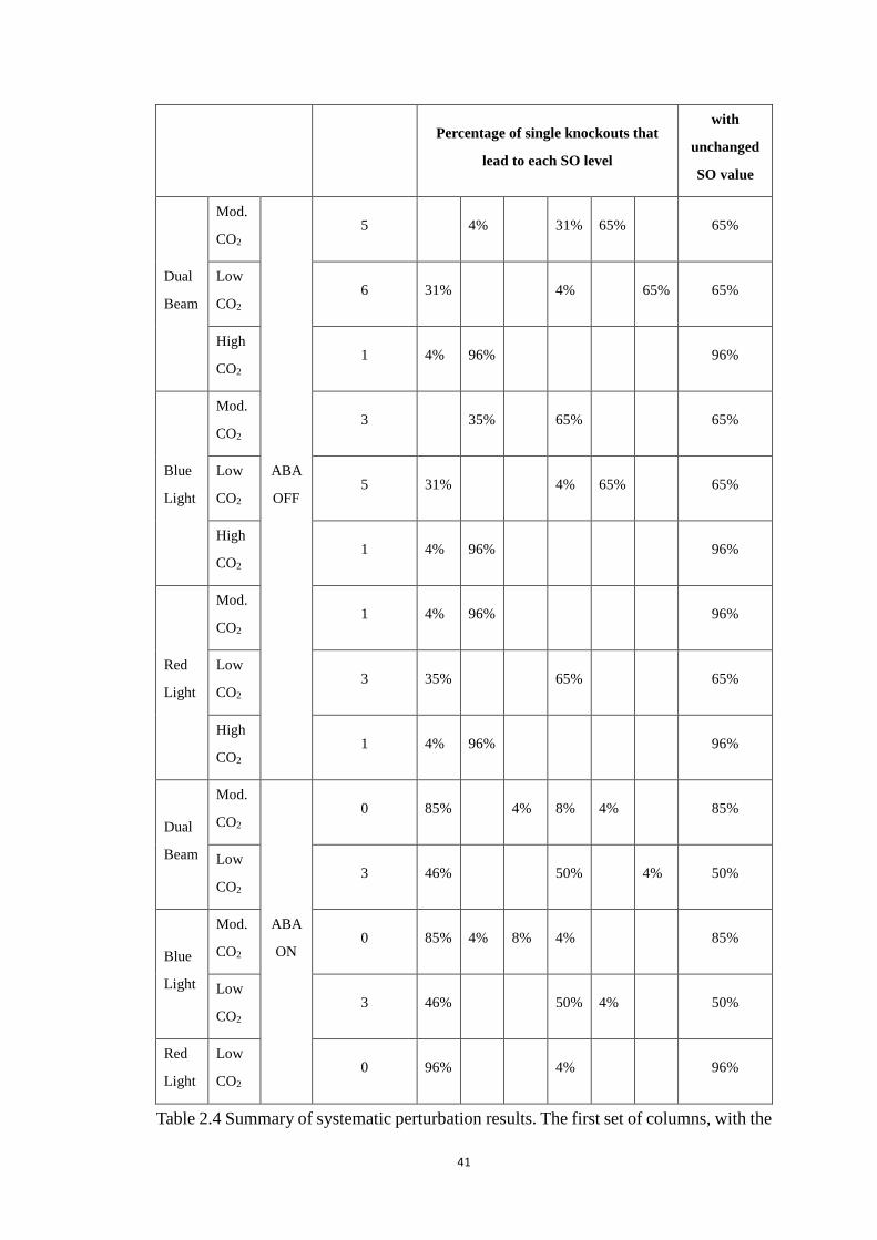
41

Percentage of single knockouts that

lead to each SO level

with

unchanged

SO value

Dual

Beam

Mod.

CO2

ABA

OFF

5 4% 31% 65% 65%

Low

CO2 6 31% 4% 65% 65%

High

CO2 1 4% 96% 96%

Blue

Light

Mod.

CO2 3 35% 65% 65%

Low

CO2 5 31% 4% 65% 65%

High

CO2 1 4% 96% 96%

Red

Light

Mod.

CO2 1 4% 96% 96%

Low

CO2 3 35% 65% 65%

High

CO2 1 4% 96% 96%

Dual

Beam

Mod.

CO2

ABA

ON

0 85% 4% 8% 4% 85%

Low

CO2 3 46% 50% 4% 50%

Blue

Light

Mod.

CO2 0 85% 4% 8% 4% 85%

Low

CO2 3 46% 50% 4% 50%

Red

Light

Low

CO2 0 96% 4% 96%

Table 2.4 Summary of systematic perturbation results. The first set of columns, with the

42

header ‘Light, CO2 and ABA condition’, indicate the input signal combinations. The

abbreviation “Mod.” means moderate CO2 concentration. Note that we do not list the

four input combinations (high CO2 with ABA and with any type of light, or moderate

CO2 with ABA and red light) wherein all simulated stomatal opening values are zero.

The 2nd column is the simulated stomatal opening (SO) level in the unperturbed system.

The 3rd column set shows the percentage of single-node knockouts that yield the

corresponding SO level. There is no stomatal opening level 4 in the reduced model. No

entry means zero percentage. The last column is the percentage of settings where the

stomatal opening remains at the same level as the unperturbed case. A complete table of

perturbation results is provided in Appendix A2.

Extending the conclusions to the original model

We found that in the reduced model there is no oscillation except in the calcium

nodes; there is no multi-stability except in the nodes PMV and Kout. Because the

reduction we used has been shown to conserve attractors [13, 14], we know that our

attractor conclusions can be immediately extended to all nodes in the original model

except the reduced nodes and stomatal opening. Next we extend the attractor analysis

to include the reduced nodes as well.

First we consider the nodes reduced during the first step of network reduction, i.e.

non-signal source nodes and simple mediator nodes. These nodes are trivially incapable

of having multi-stability and oscillations themselves, so we need only to consider their

perturbations. Perturbation of a simple mediator node can always be replaced by a

corresponding (set of) perturbation(s) in the mediator node’s direct successor(s), so

these perturbations have already been considered. Perturbing a non-signal source node

may theoretically cause a difference, however the nodes in this category in the Sun et

al. model represent molecules that are abundant in the cell or cell environment, thus

their perturbation is not biologically relevant or practical.

Next we consider the anion nodes reduced due to the simplified stomatal opening

rule. Recall that these nodes do not affect other nodes except stomatal opening in the

long term. There cannot be multi-stability in anion nodes unless the assumptions of

sufficient initial [NO3-]a and starch concentration, and sufficient initial mitochondrial

TCA cycle activity are violated (details are provided in Additional File 3 of [2], section

5 and 6). Since there is no support for interventions that would lead to the violation of

these assumptions, it is reasonable to conclude that no multi-stability can be found in

the reduced nodes under biologically relevant situations. We also found that there can

be an additional oscillation in the RIC7 path (involving the nodes ROP2, RIC7 and SO)

when a special set of perturbations is applied. Under that case, the nodes RIC7 and SO

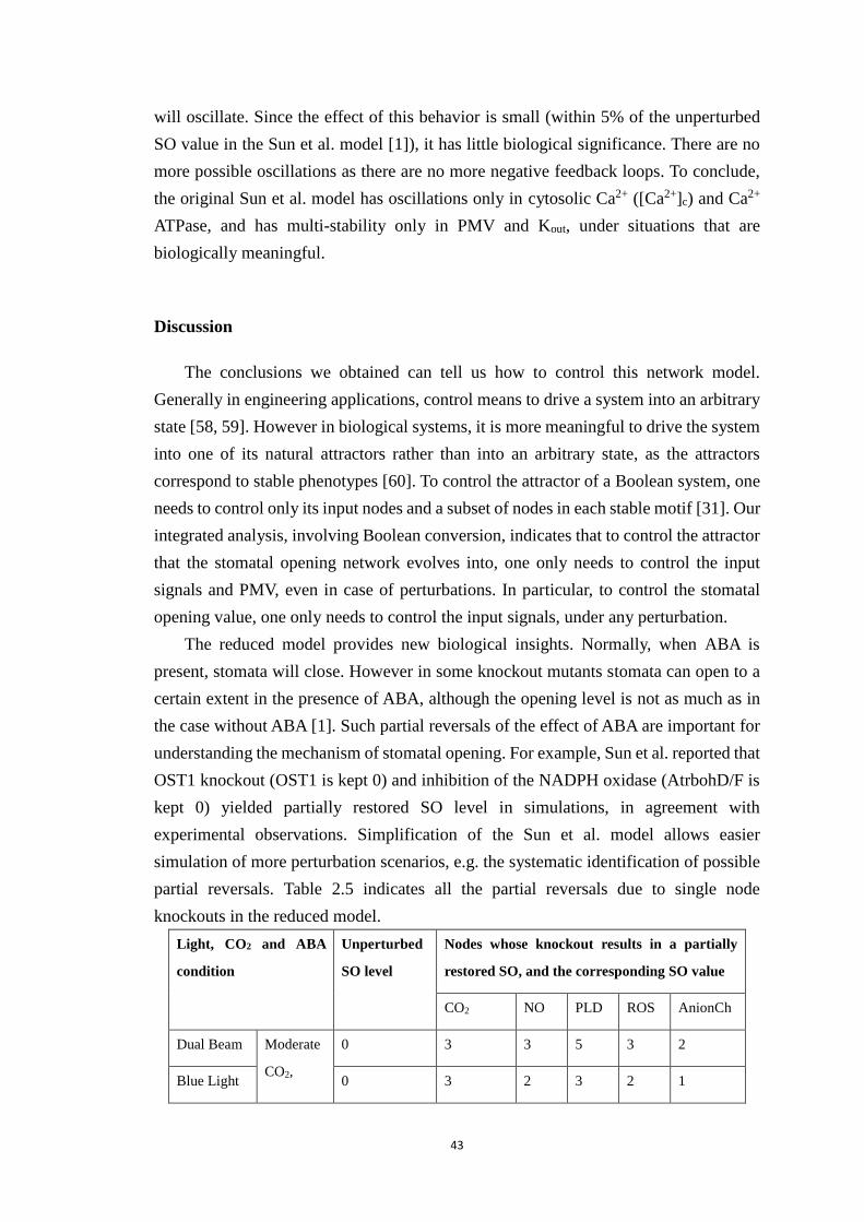
43

will oscillate. Since the effect of this behavior is small (within 5% of the unperturbed

SO value in the Sun et al. model [1]), it has little biological significance. There are no

more possible oscillations as there are no more negative feedback loops. To conclude,

the original Sun et al. model has oscillations only in cytosolic Ca2+ ([Ca2+]c) and Ca2+

ATPase, and has multi-stability only in PMV and Kout, under situations that are

biologically meaningful.

Discussion

The conclusions we obtained can tell us how to control this network model.

Generally in engineering applications, control means to drive a system into an arbitrary

state [58, 59]. However in biological systems, it is more meaningful to drive the system

into one of its natural attractors rather than into an arbitrary state, as the attractors

correspond to stable phenotypes [60]. To control the attractor of a Boolean system, one

needs to control only its input nodes and a subset of nodes in each stable motif [31]. Our

integrated analysis, involving Boolean conversion, indicates that to control the attractor

that the stomatal opening network evolves into, one only needs to control the input

signals and PMV, even in case of perturbations. In particular, to control the stomatal

opening value, one only needs to control the input signals, under any perturbation.

The reduced model provides new biological insights. Normally, when ABA is

present, stomata will close. However in some knockout mutants stomata can open to a

certain extent in the presence of ABA, although the opening level is not as much as in

the case without ABA [1]. Such partial reversals of the effect of ABA are important for

understanding the mechanism of stomatal opening. For example, Sun et al. reported that

OST1 knockout (OST1 is kept 0) and inhibition of the NADPH oxidase (AtrbohD/F is

kept 0) yielded partially restored SO level in simulations, in agreement with

experimental observations. Simplification of the Sun et al. model allows easier

simulation of more perturbation scenarios, e.g. the systematic identification of possible

partial reversals. Table 2.5 indicates all the partial reversals due to single node

knockouts in the reduced model.

Light, CO2 and ABA

condition

Unperturbed

SO level

Nodes whose knockout results in a partially

restored SO, and the corresponding SO value

CO2 NO PLD ROS AnionCh

Dual Beam Moderate

CO2,

0 3 3 5 3 2

Blue Light 0 3 2 3 2 1

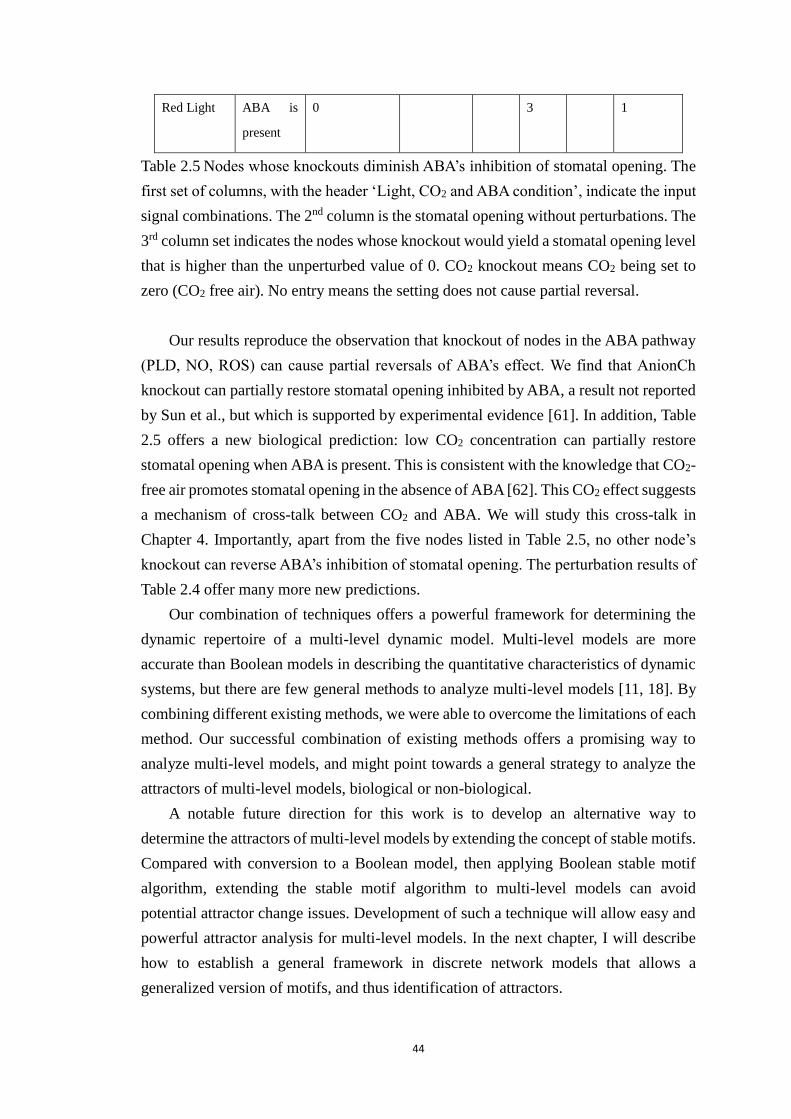
44

Red Light ABA is

present

0 3 1

Table 2.5 Nodes whose knockouts diminish ABA’s inhibition of stomatal opening. The

first set of columns, with the header ‘Light, CO2 and ABA condition’, indicate the input

signal combinations. The 2nd column is the stomatal opening without perturbations. The

3rd column set indicates the nodes whose knockout would yield a stomatal opening level

that is higher than the unperturbed value of 0. CO2 knockout means CO2 being set to

zero (CO2 free air). No entry means the setting does not cause partial reversal.

Our results reproduce the observation that knockout of nodes in the ABA pathway

(PLD, NO, ROS) can cause partial reversals of ABA’s effect. We find that AnionCh

knockout can partially restore stomatal opening inhibited by ABA, a result not reported

by Sun et al., but which is supported by experimental evidence [61]. In addition, Table

2.5 offers a new biological prediction: low CO2 concentration can partially restore

stomatal opening when ABA is present. This is consistent with the knowledge that CO2-

free air promotes stomatal opening in the absence of ABA [62]. This CO2 effect suggests

a mechanism of cross-talk between CO2 and ABA. We will study this cross-talk in

Chapter 4. Importantly, apart from the five nodes listed in Table 2.5, no other node’s

knockout can reverse ABA’s inhibition of stomatal opening. The perturbation results of

Table 2.4 offer many more new predictions.

Our combination of techniques offers a powerful framework for determining the

dynamic repertoire of a multi-level dynamic model. Multi-level models are more

accurate than Boolean models in describing the quantitative characteristics of dynamic

systems, but there are few general methods to analyze multi-level models [11, 18]. By

combining different existing methods, we were able to overcome the limitations of each

method. Our successful combination of existing methods offers a promising way to

analyze multi-level models, and might point towards a general strategy to analyze the

attractors of multi-level models, biological or non-biological.

A notable future direction for this work is to develop an alternative way to

determine the attractors of multi-level models by extending the concept of stable motifs.

Compared with conversion to a Boolean model, then applying Boolean stable motif

algorithm, extending the stable motif algorithm to multi-level models can avoid

potential attractor change issues. Development of such a technique will allow easy and

powerful attractor analysis for multi-level models. In the next chapter, I will describe

how to establish a general framework in discrete network models that allows a

generalized version of motifs, and thus identification of attractors.

45

Chapter 3 A general method to find the attractors of

discrete dynamic models of biological systems

Most of this chapter is based on previously published work for which I am the first

author [33]. Parts of the published work are reproduced in this chapter from Phys Rev

E, 2018. 97(4-1), Copyright 2018 APS.

Introduction

Dynamic modeling is a valuable avenue for understanding the emergent properties of

interacting biological systems [63, 64]. Networks, with their nodes representing

biological entities and their edges representing interactions, can connect the interactions

among cellular constituents (e.g. mRNAs, proteins or small molecules) to cell-level

functions or behaviors [44, 65]. Once a network is constructed, a dynamic model can be

created next. Each node is characterized with a state variable, representing its abundance,

concentration or activation level [40]. The state variable will evolve over time according

to a regulatory function that depends on the regulators of the node. The state variables

and regulatory functions of a dynamic model can be discrete or continuous. Discrete

modeling is particularly powerful in biological models in that it can capture the system’s

behavior without the need for much kinetic detail [66-68]. Such detail, including

reaction stoichiometry and kinetic rates, is often difficult to obtain in experiments, and

for most systems, especially large networks, the existing knowledge is insufficient to

effectively inform continuous models [69]. In this work we focus on discrete dynamic

models.

Attractors are long-term behaviors of a dynamic system, and represent system-level

outcomes. They are especially important for biological systems because they represent

biological phenotypes. For example, in a cell signaling network, attractors can

correspond to cell types, cell fates or behaviors, including cyclic behaviors such as

circadian rhythms and the cell cycle [22, 70]. Therefore, finding the attractor repertoire

of a network model is an important goal. However finding all attractors (including cyclic

and complex attractors) is challenging due to the complex dynamics of networks [71].

Thanks to the strong advances in understanding network structure [72-75], a promising

way to tackle this problem is to try to find the attractors based on the network topology

and the key features of the network’s dynamics, instead of from its detailed dynamics

[76]. For example, R. Thomas related the conditions of multi-stability and cyclic

attractors to positive and negative feedback loops, respectively [3]. Boolean models,

46

which characterize each node with two states and describe regulation in a parameter-

free manner, are most strongly based on the network structure. Many methods exist for

finding attractors of Boolean networks [56, 77-79]. Although for some systems Boolean

modeling is appropriate, often at least a subset of the nodes needs to be characterized

by multiple levels, in order to accurately describe experimentally observed relative

outcomes in case of combinations of inputs [80, 81]. For example, multiple elements of

the signal transduction network that underlies light-induced opening of microscopic

pores on plant leaves were observed to have different activity levels under red light,

blue light, and white (combined) light [1]. Three levels also allow the separate

representation of upregulation or downregulation compared to a baseline/normal level

[82]. Current approaches to attractor (mainly fixed point) identification in multi-level

models use exhaustive search, model checking methods or polynomial algebra [18, 83,

84]. Yet, there is still an unmet need for a general method that can effectively find all

attractors (fixed points and complex attractors) of a multi-level model.

In this chapter, we propose a general method that can find both fixed points and

complex attractors of any finite multi-level model. Our method is an extension of a

Boolean attractor finding method proposed by Zañudo & Albert [30]. We test and

validate our method on synthetic networks and on a collection of biological models from

the literature.

Methods

In this section we give background information on discrete dynamic modeling and

attractors, and then an overview of our method. In sub-sections C to I we describe each

step of the method in detail.

A. Discrete dynamic modeling and attractors

Discrete dynamic models require minimal parameterization, yet they can capture

important biological emergent properties, and are widely used in describing biological

networks [71, 85]. These models use discrete time (implemented through update

schemes). There are deterministic update schemes such as synchronous update, where

all nodes are updated simultaneously at each time step according to their regulatory

function [42], or asynchronous schemes with fixed time delays [86]; there are also

stochastic update schemes [87], for example a general asynchronous update where in

each time step, one node from the network is randomly chosen to update [88]. By

considering multiple replicate simulations, general asynchronous update in effect

samples all kinds of rates. It is motivated by the fact that the temporal details of

47

biological processes are difficult to obtain and usually insufficiently known. By

considering every kind of rates of states transitions, this update method is capable of

covering multiple timescales involved in intracellular processes, making up for

incomplete knowledge of the reaction timescales in biological network modeling, while

synchronous update can lead to spurious behaviors [89]. Therefore it is applied

frequently in biological models, in both simulations [90] and theoretical analysis [26,

28].

An attractor can be described as one of the smallest self-contained set of states, i.e. a

set of states from which only states in the same set can be reached. Attractors include

steady state attractors (fixed points), and complex (oscillating) attractors where a subset

of the nodes do not take fixed values. In discrete models, attractors can also be defined

as the terminal strongly-connected-components (SCCs) of the state transition graph

(STG). An STG of a dynamic model is the graph wherein each node represents a state

of the system, and each edge represents a state transition. The nodes in a terminal SCC

of the STG are self-contained as they cannot reach nodes other than themselves, and are

therefore attractors of the system.

In a discrete dynamical system, the fixed point attractors are independent of the

update scheme; on the other hand, complex attractors may depend on the update scheme

of the system. This is intuitive, as the edges of a STG can be different for different

update schemes. An example is provided in Appendix B4. Since the general

asynchronous update allow all kinds of rates and timing, complex attractors found under

general asynchronous update are invariant with respect to arbitrary fluctuations in the

rates of the processes involved [91]. In this chapter, we will focus on general

asynchronous update.

An accurate method to find all attractors of discrete models is to perform an

exhaustive search in the state space. However this is not practical because the state space

of a network scales exponentially with its size. Even for the simplest, Boolean model,

the size of the state space of an N-node network is 2N, which is too large for exhaustive

search. There has been a lot of effort to develop methods to find attractors in the Boolean

framework [56, 77-79], but there are only a few methods that can find attractors of

multi-level models, and they have special constrains when finding complex attractors.

For example, Dubrova et al. proposed an SAT-based bounded model checking method

that can only find complex attractors in a synchronous update scheme [83]. Hinkelmann

et al. converted the attractor finding problem into solving polynomial equations; this

method can only find complex attractors of a limited size [84]. Our method does not

explicitly consider time and does not enumerate the system’s trajectories. Instead, it

combines graph topology and regulatory functions into an expanded graph

48

representation. Because this expanded network is much smaller than the size of the state

space, our method can work on networks of larger size. Our method is comprehensive

in the broad family of dynamical systems wherein one node changes state at any given

time instant.

B. Overview of our motif-based attractor identification method

The idea of our method is to translate the attractor identification problem into a graph

theoretical problem by creating an expanded representation of the network that

incorporates all the regulatory functions, then identifying certain motifs (subgraphs) of

this expanded network [92]. We will refer to our method as the motif-based attractor

identification method, or ‘motif-based method’ for short.

We first represent each state of each original node with a Boolean virtual node. The

‘ON’ state of the virtual node means that the original node is in the state embodied by

the virtual node. The regulatory function of a virtual node is a quasi-Boolean function,

whose inputs are virtual nodes, expressed in an appropriate disjunctive normal form.

This disjunctive normal form is obtained by summing up the input combinations that

yield the ‘ON’ state for the virtual node.

Then an expanded network containing all information expressed in the regulatory

functions can be established. The expanded network is obtained from the original one

by the following operations: 1. Include each virtual node in the expanded network, and

connect all the virtual node’s regulators to it; 2. for each ‘and’ rule in the regulatory

functions, create a composite node, and re-wire the edges from the input nodes of the

‘and’ rule to this composite node, then connect the composite node to the regulated

(target) node. The original edges from the input nodes of the ‘and’ rule to the target node

are removed. The expanded network allows one to distinguish between co-pointing

interactions that are combinatorial in nature (i.e. they are combined by ‘and’ rules) from

co-pointing interactions that are individually sufficient (i.e. they are combined by ‘or’

rules).

We use the term “motif” for strongly connected components of the expanded network

that satisfy certain properties (which we will describe later). Depending on the virtual

nodes involved in the motif, we define stable motifs, which correspond to stabilized

states of the constituent nodes, and oscillating motifs, which are candidates for

oscillations of the constituent nodes.

After the motifs are found, plugging in the node states specified in the motifs into the

regulatory functions of their target nodes will specify the states of these nodes, therefore

reducing the network. Then more motifs can be found in the reduced network, and this

reduction process can be done iteratively. Ultimately, the motif sequence we find in the

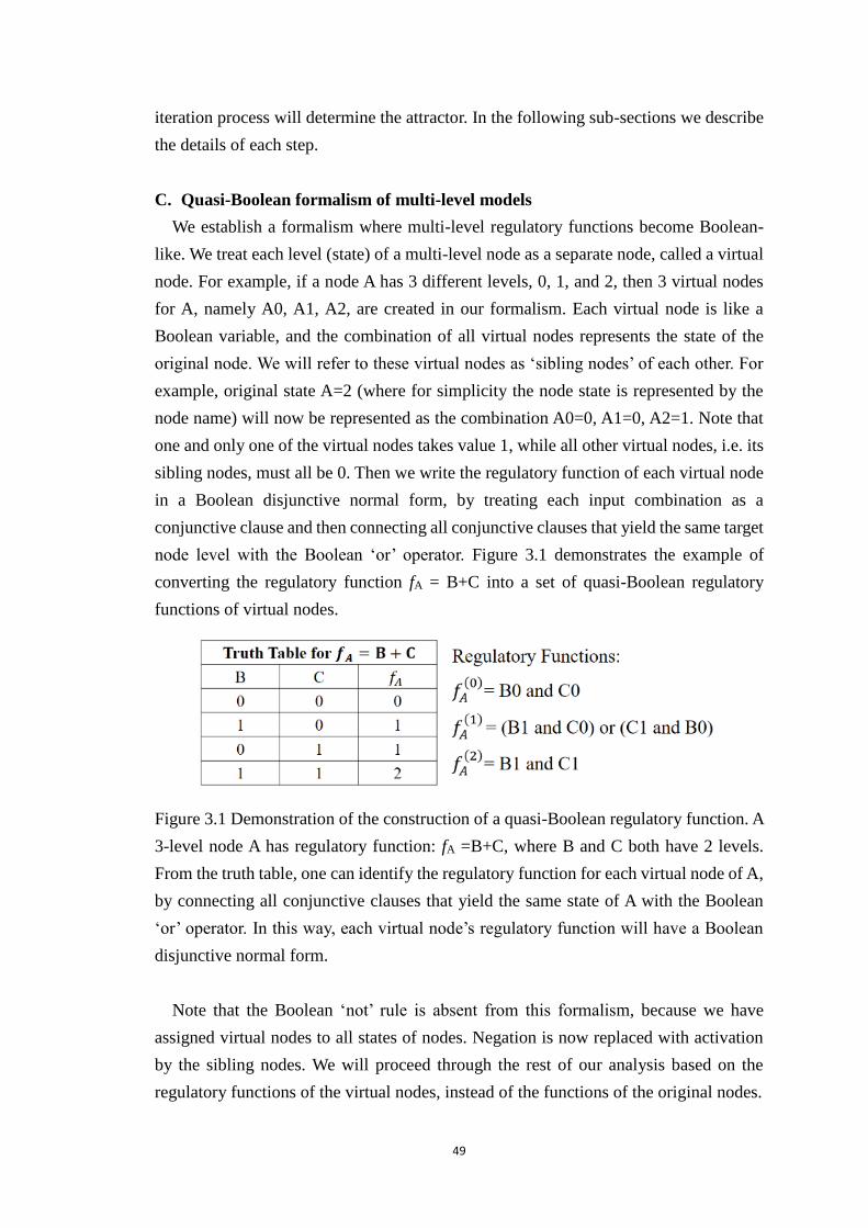
49

iteration process will determine the attractor. In the following sub-sections we describe

the details of each step.

C. Quasi-Boolean formalism of multi-level models

We establish a formalism where multi-level regulatory functions become Boolean-

like. We treat each level (state) of a multi-level node as a separate node, called a virtual

node. For example, if a node A has 3 different levels, 0, 1, and 2, then 3 virtual nodes

for A, namely A0, A1, A2, are created in our formalism. Each virtual node is like a

Boolean variable, and the combination of all virtual nodes represents the state of the

original node. We will refer to these virtual nodes as ‘sibling nodes’ of each other. For

example, original state A=2 (where for simplicity the node state is represented by the

node name) will now be represented as the combination A0=0, A1=0, A2=1. Note that

one and only one of the virtual nodes takes value 1, while all other virtual nodes, i.e. its

sibling nodes, must all be 0. Then we write the regulatory function of each virtual node

in a Boolean disjunctive normal form, by treating each input combination as a

conjunctive clause and then connecting all conjunctive clauses that yield the same target

node level with the Boolean ‘or’ operator. Figure 3.1 demonstrates the example of

converting the regulatory function fA = B+C into a set of quasi-Boolean regulatory

functions of virtual nodes.

Figure 3.1 Demonstration of the construction of a quasi-Boolean regulatory function. A

3-level node A has regulatory function: fA =B+C, where B and C both have 2 levels.

From the truth table, one can identify the regulatory function for each virtual node of A,

by connecting all conjunctive clauses that yield the same state of A with the Boolean

‘or’ operator. In this way, each virtual node’s regulatory function will have a Boolean

disjunctive normal form.

Note that the Boolean ‘not’ rule is absent from this formalism, because we have

assigned virtual nodes to all states of nodes. Negation is now replaced with activation

by the sibling nodes. We will proceed through the rest of our analysis based on the

regulatory functions of the virtual nodes, instead of the functions of the original nodes.

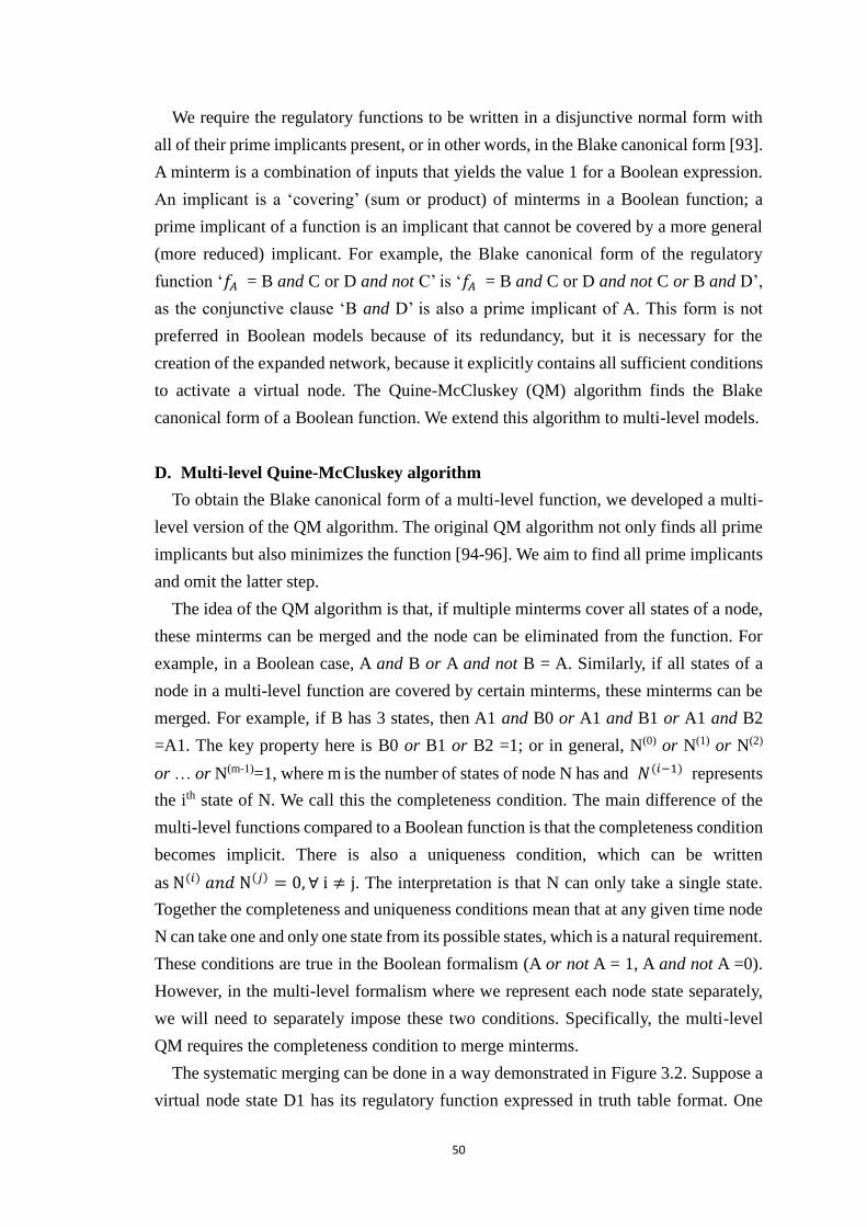
50

We require the regulatory functions to be written in a disjunctive normal form with

all of their prime implicants present, or in other words, in the Blake canonical form [93].

A minterm is a combination of inputs that yields the value 1 for a Boolean expression.

An implicant is a ‘covering’ (sum or product) of minterms in a Boolean function; a

prime implicant of a function is an implicant that cannot be covered by a more general

(more reduced) implicant. For example, the Blake canonical form of the regulatory

function ‘𝑓𝐴 = B and C or D and not C’ is ‘𝑓𝐴 = B and C or D and not C or B and D’,

as the conjunctive clause ‘B and D’ is also a prime implicant of A. This form is not

preferred in Boolean models because of its redundancy, but it is necessary for the

creation of the expanded network, because it explicitly contains all sufficient conditions

to activate a virtual node. The Quine-McCluskey (QM) algorithm finds the Blake

canonical form of a Boolean function. We extend this algorithm to multi-level models.

D. Multi-level Quine-McCluskey algorithm

To obtain the Blake canonical form of a multi-level function, we developed a multi-

level version of the QM algorithm. The original QM algorithm not only finds all prime

implicants but also minimizes the function [94-96]. We aim to find all prime implicants

and omit the latter step.

The idea of the QM algorithm is that, if multiple minterms cover all states of a node,

these minterms can be merged and the node can be eliminated from the function. For

example, in a Boolean case, A and B or A and not B = A. Similarly, if all states of a

node in a multi-level function are covered by certain minterms, these minterms can be

merged. For example, if B has 3 states, then A1 and B0 or A1 and B1 or A1 and B2

=A1. The key property here is B0 or B1 or B2 =1; or in general, N(0) or N(1) or N(2)

or … or N(m-1)=1, where m is the number of states of node N has and 𝑁(𝑖−1) represents

the ith state of N. We call this the completeness condition. The main difference of the

multi-level functions compared to a Boolean function is that the completeness condition

becomes implicit. There is also a uniqueness condition, which can be written

as N(𝑖) 𝑎𝑛𝑑 N(𝑗) = 0, ∀ i ≠ j. The interpretation is that N can only take a single state.

Together the completeness and uniqueness conditions mean that at any given time node

N can take one and only one state from its possible states, which is a natural requirement.

These conditions are true in the Boolean formalism (A or not A = 1, A and not A =0).

However, in the multi-level formalism where we represent each node state separately,

we will need to separately impose these two conditions. Specifically, the multi-level

QM requires the completeness condition to merge minterms.

The systematic merging can be done in a way demonstrated in Figure 3.2. Suppose a

virtual node state D1 has its regulatory function expressed in truth table format. One

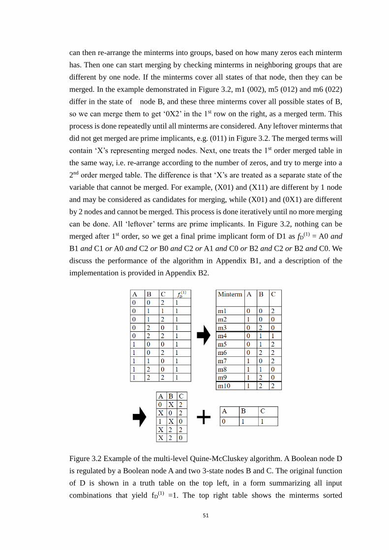
51

can then re-arrange the minterms into groups, based on how many zeros each minterm

has. Then one can start merging by checking minterms in neighboring groups that are

different by one node. If the minterms cover all states of that node, then they can be

merged. In the example demonstrated in Figure 3.2, m1 (002), m5 (012) and m6 (022)

differ in the state of node B, and these three minterms cover all possible states of B,

so we can merge them to get ‘0X2’ in the 1st row on the right, as a merged term. This

process is done repeatedly until all minterms are considered. Any leftover minterms that

did not get merged are prime implicants, e.g. (011) in Figure 3.2. The merged terms will

contain ‘X’s representing merged nodes. Next, one treats the 1st order merged table in

the same way, i.e. re-arrange according to the number of zeros, and try to merge into a

2nd order merged table. The difference is that ‘X’s are treated as a separate state of the

variable that cannot be merged. For example, (X01) and (X11) are different by 1 node

and may be considered as candidates for merging, while (X01) and (0X1) are different

by 2 nodes and cannot be merged. This process is done iteratively until no more merging

can be done. All ‘leftover’ terms are prime implicants. In Figure 3.2, nothing can be

merged after 1st order, so we get a final prime implicant form of D1 as fD(1) = A0 and

B1 and C1 or A0 and C2 or B0 and C2 or A1 and C0 or B2 and C2 or B2 and C0. We

discuss the performance of the algorithm in Appendix B1, and a description of the

implementation is provided in Appendix B2.

Figure 3.2 Example of the multi-level Quine-McCluskey algorithm. A Boolean node D

is regulated by a Boolean node A and two 3-state nodes B and C. The original function

of D is shown in a truth table on the top left, in a form summarizing all input

combinations that yield fD(1) =1. The top right table shows the minterms sorted

52

according to the number of zeros in them. From this table, one can merge the terms

between layers that are different by 1 digit, if all states of the difference node are present

within the two layers. The result of the merging is shown below. Merged terms are

represented by an ‘X’. There are 5 leftover terms after 1st order merging, and there is 1

leftover term after 0th order merging. The sum of all six terms is the final expression.

E. The expanded network representation

After all functions are transformed into the proper form, we create an expanded

network, which is a representation of the network with regulatory functions embedded.

The expanded network is obtained from the original network by applying the following

operations: 1. Include each virtual node in the expanded network, and connect its

regulators to it; 2. for each ‘and’ rule in the regulatory functions, create a composite

node, and re-wire the edges from the input nodes of the ‘and’ rule to this composite node,

then connect the composite node to the regulated node. The original edges from input

nodes of the ‘and’ rule to the target node are removed. Figure 3.3 exemplifies the

construction of an expanded network from a regulatory function. To construct the entire

expanded network, all virtual nodes and all interactions must be created.

Figure 3.3 Construction of an expanded network from a regulatory function. Virtual

node A0 has function fA(0) = B0 or (C1 and B1), so in the expanded network, B0 is

connected directly to A0; C1 and B1 are connected indirectly to A0 via composite node

'C1 and B1'. A1 has function fA(1) = C0 and B1, so C0 and B1 are connected indirectly

to A0 via composite node 'C0 and B1'.

The expanded network contains not only the network structure, but also all

information about the regulatory functions. Furthermore, interactions of a combinatorial

nature are separated, as all ‘and’ rules have become explicit nodes. In this way, the

expanded network makes it easy to identify a sufficient condition to activate a node: a

virtual node will have state 1 if any of its regulator virtual nodes is 1, or if any of its

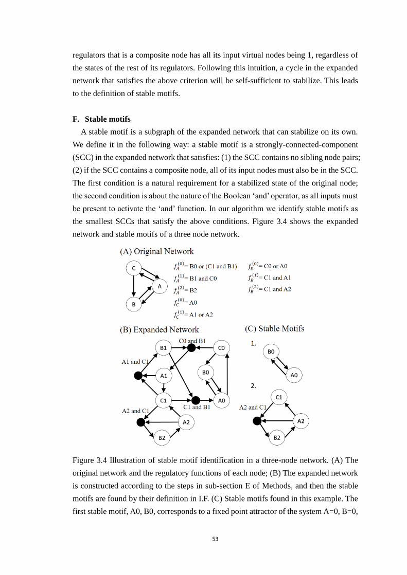
53

regulators that is a composite node has all its input virtual nodes being 1, regardless of

the states of the rest of its regulators. Following this intuition, a cycle in the expanded

network that satisfies the above criterion will be self-sufficient to stabilize. This leads

to the definition of stable motifs.

F. Stable motifs

A stable motif is a subgraph of the expanded network that can stabilize on its own.

We define it in the following way: a stable motif is a strongly-connected-component

(SCC) in the expanded network that satisfies: (1) the SCC contains no sibling node pairs;

(2) if the SCC contains a composite node, all of its input nodes must also be in the SCC.

The first condition is a natural requirement for a stabilized state of the original node;

the second condition is about the nature of the Boolean ‘and’ operator, as all inputs must

be present to activate the ‘and’ function. In our algorithm we identify stable motifs as

the smallest SCCs that satisfy the above conditions. Figure 3.4 shows the expanded

network and stable motifs of a three node network.

Figure 3.4 Illustration of stable motif identification in a three-node network. (A) The

original network and the regulatory functions of each node; (B) The expanded network

is constructed according to the steps in sub-section E of Methods, and then the stable

motifs are found by their definition in I.F. (C) Stable motifs found in this example. The

first stable motif, A0, B0, corresponds to a fixed point attractor of the system A=0, B=0,

54

C=0. The state C=0 is found by plugging A=B=0 into the regulatory function of C. The

2nd stable motif corresponds to another fixed point attractor A=2, B=2, C=0.

In order for stable motifs to be correctly recognized, the regulatory functions must

contain all prime implicants. If a prime implicant is missing, a sufficient condition for

a node to stabilize is missing, which would lead to incorrect identification of stable

motifs. This is why we require the Blake canonical form of regulatory functions.

There is a one-to-one correspondence between a stable motif and a partial fixed point

of the system (which is defined as a state in which a subset of nodes stabilize regardless

of the state of the rest of the system). The proof of this statement is provided in Appendix

B3. Consequently, by finding all stable motifs we find all fixed points or partial fixed

points of the system.

G. Oscillating motifs

An oscillating motif is defined as the largest SCC in the expanded network that

satisfies: (1) at least one virtual node in the SCC has at least one sibling node in the

SCC; (2) if the SCC contains a composite node, all its input nodes must also be in the

SCC. In contrast to nodes in stable motifs, an oscillating node must be able to enter at

least two states, so the first condition is necessary. The second condition is also

necessary due to the combinatorial nature of the composite node.

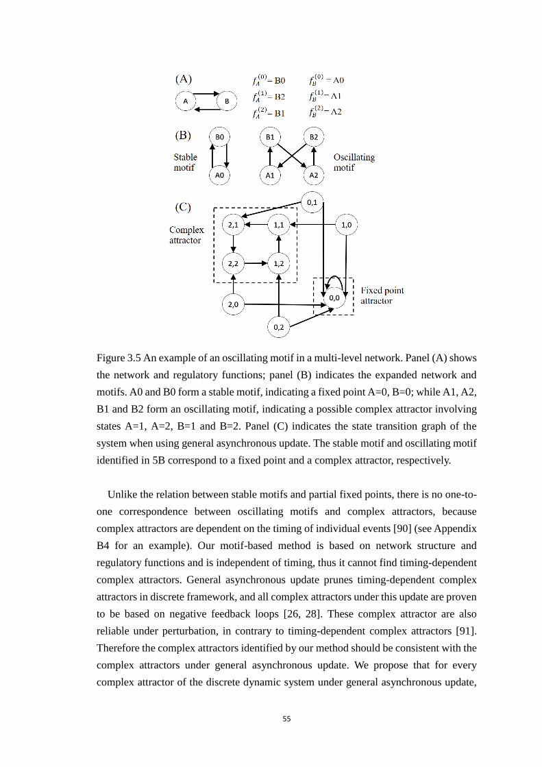
55

Figure 3.5 An example of an oscillating motif in a multi-level network. Panel (A) shows

the network and regulatory functions; panel (B) indicates the expanded network and

motifs. A0 and B0 form a stable motif, indicating a fixed point A=0, B=0; while A1, A2,

B1 and B2 form an oscillating motif, indicating a possible complex attractor involving

states A=1, A=2, B=1 and B=2. Panel (C) indicates the state transition graph of the

system when using general asynchronous update. The stable motif and oscillating motif

identified in 5B correspond to a fixed point and a complex attractor, respectively.

Unlike the relation between stable motifs and partial fixed points, there is no one-to-

one correspondence between oscillating motifs and complex attractors, because

complex attractors are dependent on the timing of individual events [90] (see Appendix

B4 for an example). Our motif-based method is based on network structure and

regulatory functions and is independent of timing, thus it cannot find timing-dependent

complex attractors. General asynchronous update prunes timing-dependent complex

attractors in discrete framework, and all complex attractors under this update are proven

to be based on negative feedback loops [26, 28]. These complex attractor are also

reliable under perturbation, in contrary to timing-dependent complex attractors [91].

Therefore the complex attractors identified by our method should be consistent with the

complex attractors under general asynchronous update. We propose that for every

complex attractor of the discrete dynamic system under general asynchronous update,

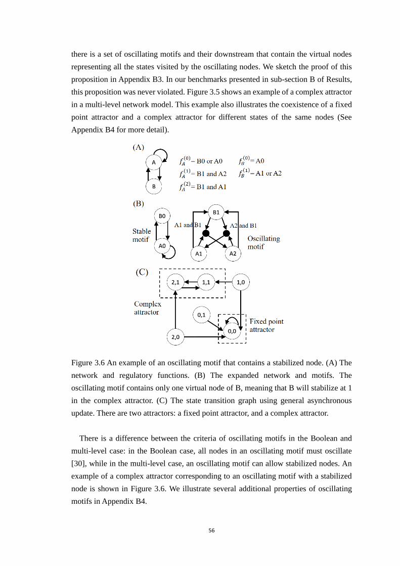
56

there is a set of oscillating motifs and their downstream that contain the virtual nodes

representing all the states visited by the oscillating nodes. We sketch the proof of this

proposition in Appendix B3. In our benchmarks presented in sub-section B of Results,

this proposition was never violated. Figure 3.5 shows an example of a complex attractor

in a multi-level network model. This example also illustrates the coexistence of a fixed

point attractor and a complex attractor for different states of the same nodes (See

Appendix B4 for more detail).

Figure 3.6 An example of an oscillating motif that contains a stabilized node. (A) The

network and regulatory functions. (B) The expanded network and motifs. The

oscillating motif contains only one virtual node of B, meaning that B will stabilize at 1

in the complex attractor. (C) The state transition graph using general asynchronous

update. There are two attractors: a fixed point attractor, and a complex attractor.

There is a difference between the criteria of oscillating motifs in the Boolean and

multi-level case: in the Boolean case, all nodes in an oscillating motif must oscillate

[30], while in the multi-level case, an oscillating motif can allow stabilized nodes. An

example of a complex attractor corresponding to an oscillating motif with a stabilized

node is shown in Figure 3.6. We illustrate several additional properties of oscillating

motifs in Appendix B4.

57

H. Iterative motif reduction yields the attractors of the system

The source (unregulated) nodes of a network that stabilize in a fixed state can be

reduced prior to any attractor identification process. The corresponding fixed states can

be substituted into the regulatory functions of the nodes they regulate. This can be done

iteratively until no source nodes are present in the network, without affecting the

attractor repertoire of the system [13, 14]. For some biological networks, this reduction

alone can reduce a large fraction of the network model, leading to a much simplified

model.

Once motifs are identified, we can plug in the states of the nodes specified in the

motifs into the expanded network, as if these nodes were source nodes, to further reduce

the network. For stabilized nodes, the stabilized virtual node takes value 1 and its sibling

nodes are set to 0; for oscillating nodes, their corresponding virtual nodes are marked

as oscillating, and their sibling nodes excluded from the oscillating motif are set to 0.

Certain nodes downstream of the motifs may stabilize as a result. In this way, a reduced

version of the network model is obtained. We then identify stable motifs and oscillating

motifs in the reduced network and substitute the corresponding virtual node values again,

until this cannot be done any more. By the end of this process all nodes will either

become a part of a motif, or be downstream of a motif and be determined by that motif,

and we will have obtained a set of motif sequences. If no oscillating motifs are found in

a motif sequence and at the end of the process the network has reduced completely, all

nodes will be stabilized, and we will have obtained a fixed point attractor. If oscillating

motifs are found in a motif sequence, at the end of the process we will find some

(possibly none) of the nodes stabilized, while some other nodes oscillating. We call this

result a quasi-attractor. Specifically, a quasi-attractor will indicate the unique state of

each stabilized node and it will give a set of states among which a potentially oscillating

node oscillates. This quasi-attractor is likely (but not guaranteed) to correspond to a

complex attractor (see Figure B.3 in Appendix for an example). Under general

asynchronous update, since all partial fixed points correspond to stable motifs, and all

complex attractors correspond to oscillating motifs, all attractors will be covered with

our motif-based method. Note that there is no exact match between the actual number

of complex attractors and the number of quasi-attractors found by our method (see

Appendix B4).

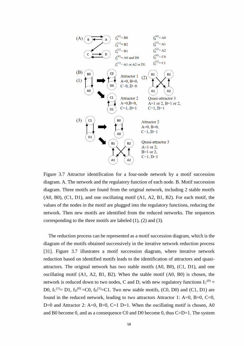
58

Figure 3.7 Attractor identification for a four-node network by a motif succession

diagram. A. The network and the regulatory function of each node. B. Motif succession

diagram. Three motifs are found from the original network, including 2 stable motifs

(A0, B0), (C1, D1), and one oscillating motif (A1, A2, B1, B2). For each motif, the

values of the nodes in the motif are plugged into the regulatory functions, reducing the

network. Then new motifs are identified from the reduced networks. The sequences

corresponding to the three motifs are labeled (1), (2) and (3).

The reduction process can be represented as a motif succession diagram, which is the

diagram of the motifs obtained successively in the iterative network reduction process

[31]. Figure 3.7 illustrates a motif succession diagram, where iterative network

reduction based on identified motifs leads to the identification of attractors and quasi-

attractors. The original network has two stable motifs (A0, B0), (C1, D1), and one

oscillating motif (A1, A2, B1, B2). When the stable motif (A0, B0) is chosen, the

network is reduced down to two nodes, C and D, with new regulatory functions fC(0) =

D0, fC(1)= D1, fD

(0) =C0, fD(1)=C1. Two new stable motifs, (C0, D0) and (C1, D1) are

found in the reduced network, leading to two attractors Attractor 1: A=0, B=0, C=0,

D=0 and Attractor 2: A=0, B=0, C=1 D=1. When the oscillating motif is chosen, A0

and B0 become 0, and as a consequence C0 and D0 become 0, thus C=D=1. The system

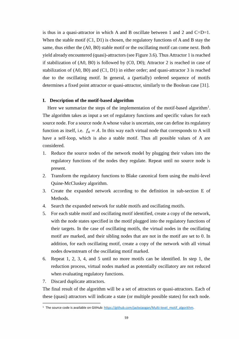
59

is thus in a quasi-attractor in which A and B oscillate between 1 and 2 and C=D=1.

When the stable motif (C1, D1) is chosen, the regulatory functions of A and B stay the

same, thus either the (A0, B0) stable motif or the oscillating motif can come next. Both

yield already encountered (quasi)-attractors (see Figure 3.6). Thus Attractor 1 is reached

if stabilization of (A0, B0) is followed by (C0, D0); Attractor 2 is reached in case of

stabilization of (A0, B0) and (C1, D1) in either order; and quasi-attractor 3 is reached

due to the oscillating motif. In general, a (partially) ordered sequence of motifs

determines a fixed point attractor or quasi-attractor, similarly to the Boolean case [31].

I. Description of the motif-based algorithm

Here we summarize the steps of the implementation of the motif-based algorithm1.

The algorithm takes as input a set of regulatory functions and specific values for each

source node. For a source node A whose value is uncertain, one can define its regulatory

function as itself, i.e. 𝑓𝐴 = 𝐴. In this way each virtual node that corresponds to A will

have a self-loop, which is also a stable motif. Thus all possible values of A are

considered.

1. Reduce the source nodes of the network model by plugging their values into the

regulatory functions of the nodes they regulate. Repeat until no source node is

present.

2. Transform the regulatory functions to Blake canonical form using the multi-level

Quine-McCluskey algorithm.

3. Create the expanded network according to the definition in sub-section E of

Methods.

4. Search the expanded network for stable motifs and oscillating motifs.

5. For each stable motif and oscillating motif identified, create a copy of the network,

with the node states specified in the motif plugged into the regulatory functions of

their targets. In the case of oscillating motifs, the virtual nodes in the oscillating

motif are marked, and their sibling nodes that are not in the motif are set to 0. In

addition, for each oscillating motif, create a copy of the network with all virtual

nodes downstream of the oscillating motif marked.

6. Repeat 1, 2, 3, 4, and 5 until no more motifs can be identified. In step 1, the

reduction process, virtual nodes marked as potentially oscillatory are not reduced

when evaluating regulatory functions.

7. Discard duplicate attractors.

The final result of the algorithm will be a set of attractors or quasi-attractors. Each of

these (quasi) attractors will indicate a state (or multiple possible states) for each node.

1 The source code is available on GitHub: https://github.com/jackxiaogan/Multi-level_motif_algorithm.

60

For each stabilized node, its unique stabilized state is given; for a potentially oscillating

node, the multiple states among which it potentially oscillates are given.

Results

To test the effectiveness of our motif-based attractor identification method, we apply

it to an ensemble of synthetic networks and biological networks from the literature.

A. Benchmark on synthetic networks

We test the motif-based algorithm on synthetic networks of different size, ranging

from 10 to 40. To approximate biological networks, we first generate networks where

the in-degree is k=2 for each node and the network is otherwise random [41, 97]. Next,

we generate the number of states for each node. For multi-level ensembles, we generate

number of states according to an equal probability of having 2 or 3 states. For Boolean

ensembles all nodes have 2 states. Then we randomly generate a regulatory function

among those consistent with the number of regulators and number of states for each

node. The generation process of regulatory functions is described in Appendix B5.

To test whether the motif-based algorithm finds attractors correctly, we perform

simulations similar to Wang et al. [98] and Zañudo et al. [30]. We start from different

random initial conditions, and let the system evolve for Tstep effective time steps. We

used general asynchronous update, where at each time step, one node is randomly

chosen and its state is updated according to its regulatory function. If the new state of

the node is the same as before, another node will be selected within the same time step,

until the selected node changes state. If no node can reach a new state, a fixed point

attractor is reached. If no fixed point attractor is reached within Tstep effective time steps,

we evaluate whether the system is in a complex attractor by determining the

corresponding partial state transition graph (STG). Note that this sampling method is

heuristic, and is likely to miss attractors when the state space is large. For each fixed

point attractor found by simulation, we check whether it is predicted by our motif-based

algorithm. In addition, for each predicted fixed point or partial fixed point we check

whether there is a simulated attractor that contains the same stabilized nodes in the same

states. If a pair of predicted and simulated fixed points passes both checks, we categorize

them as identical. If a predicted partial fixed point passes the second check, we call it

consistent with the simulated attractor. Complex attractors depend on the update scheme

(i.e. on the timing), so there cannot be a definitive conclusion. The expectation (based

on our proposition presented in sub-section G of Methods) is that the set of nodes found

to oscillate in a simulation should be a subset of the nodes predicted to oscillate by our

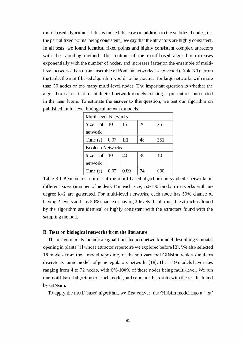
61

motif-based algorithm. If this is indeed the case (in addition to the stabilized nodes, i.e.

the partial fixed points, being consistent), we say that the attractors are highly consistent.

In all tests, we found identical fixed points and highly consistent complex attractors

with the sampling method. The runtime of the motif-based algorithm increases

exponentially with the number of nodes, and increases faster on the ensemble of multi-

level networks than on an ensemble of Boolean networks, as expected (Table 3.1). From

the table, the motif-based algorithm would not be practical for large networks with more

than 50 nodes or too many multi-level nodes. The important question is whether the

algorithm is practical for biological network models existing at present or constructed

in the near future. To estimate the answer to this question, we test our algorithm on

published multi-level biological network models.

Multi-level Networks

Size of

network

10 15 20 25

Time (s) 0.07 1.1 48 251

Boolean Networks

Size of

network

10 20 30 40

Time (s) 0.07 0.89 74 600

Table 3.1 Benchmark runtime of the motif-based algorithm on synthetic networks of

different sizes (number of nodes). For each size, 50-100 random networks with in-

degree k=2 are generated. For multi-level networks, each node has 50% chance of

having 2 levels and has 50% chance of having 3 levels. In all runs, the attractors found

by the algorithm are identical or highly consistent with the attractors found with the

sampling method.

B. Tests on biological networks from the literature

The tested models include a signal transduction network model describing stomatal

opening in plants [1] whose attractor repertoire we explored before [2]. We also selected

18 models from the model repository of the software tool GINsim, which simulates

discrete dynamic models of gene regulatory networks [18]. These 19 models have sizes

ranging from 4 to 72 nodes, with 6%-100% of these nodes being multi-level. We run

our motif-based algorithm on each model, and compare the results with the results found

by GINsim.

To apply the motif-based algorithm, we first convert the GINsim model into a ‘.txt’

62

file, with regulatory functions suitable for our algorithm2. In the few cases where the

GINsim framework and our framework are different, we adapt the model to our

framework. For example, GINsim allows an ‘empty function’: ‘fA(0) = B0, fA

(2)=B1, fA(1)

is empty, i.e. A1 has no function’, which our method doesn’t allow. In this GINsim

example, ‘A1’ will be visited transiently when node A changes from A0 to A2. We

discard the state ‘A1’. We can do so because such transient states are never part of an

attractor. We also reduce some of the large models before applying our algorithm. The

reduction consists of three methods: removing output nodes (nodes with no outgoing

edges), removing simple mediator nodes (nodes with one incoming edges and one

outgoing edge), and replacing input trees (acyclic sub-networks that contain a source

node) with a single source node. These reductions are known to conserve the attractors

of the model [13, 14]. In cases where there are a lot of different signal (source node)

state combinations, it is not practical to compare all the fixed points found. Instead, we

select representative signal combinations corresponding to different biological

phenotypes (some of which are indicated as pre-made selections in GINsim), or signal

combinations that result in different attractors.

We compare the attractor analysis results by first checking whether the fixed points

are identical, and then checking whether the complex attractors are consistent. We find

that the fixed points found by the two algorithms are identical, as expected. For complex

attractors, it is difficult to get a definite conclusion. GINsim cannot predict complex

attractors; it can only simulate the state transition graph (STG) or hierarchical transition

graph (HTG) and find the strongly-connected-component from the STG/HTG [99]. The

complexity of this method goes up quickly with the increase of the model size. Our

method can only predict quasi-attractors, which may or may not be actual complex

attractors. Therefore it is impossible to know the complex attractors exactly unless an

exhaustive (partial) state space search is performed. If the model is simple enough for

GINsim to construct an STG, we check whether the complex attractors found from the

STGs are covered by the candidates predicted by our algorithm. We found consistent

complex attractor results from the two algorithms: all complex attractors found in

simulations are covered by predicted quasi-attractors. The detailed results can be found

in the Supplementary File S1 of [33].

We also compared the runtime of the two algorithms. For the motif-based algorithm,

we record the runtime for each signal combination, then average them. GINsim does

not show the actual time spent in computation, so we only record whether the

computation completed, and give an estimated time. Note that both algorithms are

2 The converted models are uploaded to the ‘models’ folder in: https://github.com/jackxiaogan/Multi-level_motif_algorithm/.

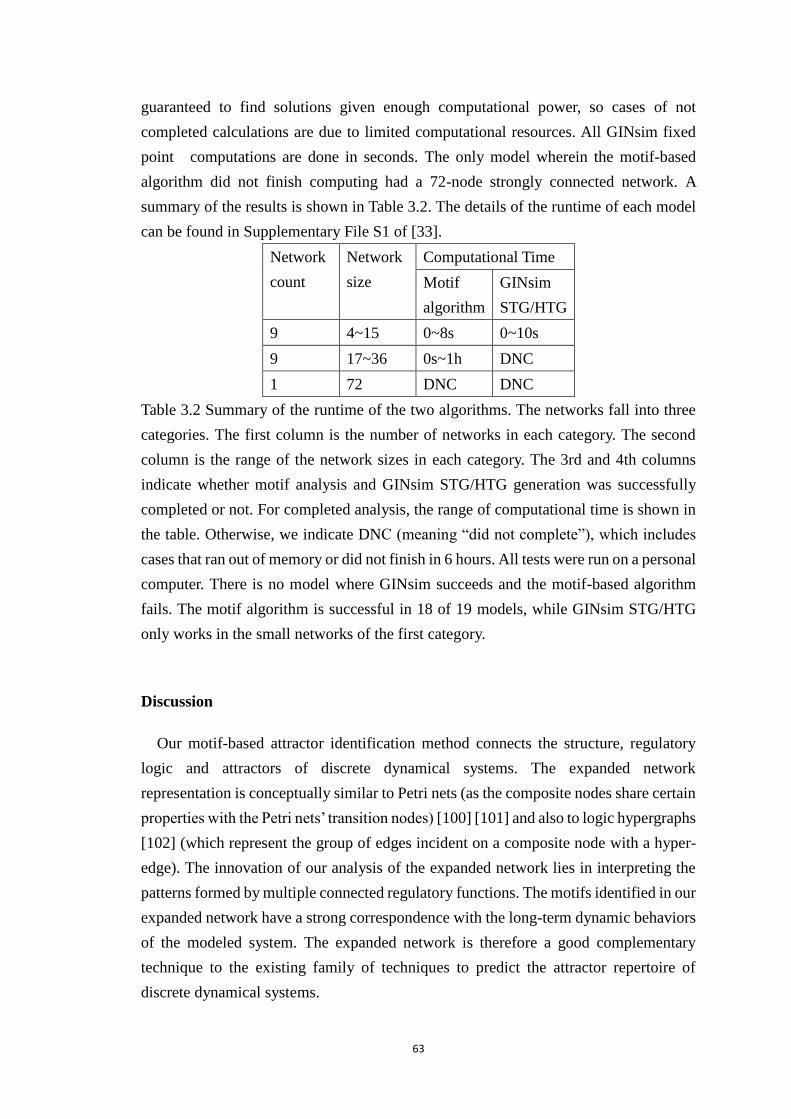
63

guaranteed to find solutions given enough computational power, so cases of not

completed calculations are due to limited computational resources. All GINsim fixed

point computations are done in seconds. The only model wherein the motif-based

algorithm did not finish computing had a 72-node strongly connected network. A

summary of the results is shown in Table 3.2. The details of the runtime of each model

can be found in Supplementary File S1 of [33].

Network

count

Network

size

Computational Time

Motif

algorithm

GINsim

STG/HTG

9 4~15 0~8s 0~10s

9 17~36 0s~1h DNC

1 72 DNC DNC

Table 3.2 Summary of the runtime of the two algorithms. The networks fall into three

categories. The first column is the number of networks in each category. The second

column is the range of the network sizes in each category. The 3rd and 4th columns

indicate whether motif analysis and GINsim STG/HTG generation was successfully

completed or not. For completed analysis, the range of computational time is shown in

the table. Otherwise, we indicate DNC (meaning “did not complete”), which includes

cases that ran out of memory or did not finish in 6 hours. All tests were run on a personal

computer. There is no model where GINsim succeeds and the motif-based algorithm

fails. The motif algorithm is successful in 18 of 19 models, while GINsim STG/HTG

only works in the small networks of the first category.

Discussion

Our motif-based attractor identification method connects the structure, regulatory

logic and attractors of discrete dynamical systems. The expanded network

representation is conceptually similar to Petri nets (as the composite nodes share certain

properties with the Petri nets’ transition nodes) [100] [101] and also to logic hypergraphs

[102] (which represent the group of edges incident on a composite node with a hyper-

edge). The innovation of our analysis of the expanded network lies in interpreting the

patterns formed by multiple connected regulatory functions. The motifs identified in our

expanded network have a strong correspondence with the long-term dynamic behaviors

of the modeled system. The expanded network is therefore a good complementary

technique to the existing family of techniques to predict the attractor repertoire of

discrete dynamical systems.

64

Our method captures not only fixed points, but also complex attractors. The fixed

points of a dynamic system are independent of timing, and will be found accurately.

Complex attractors may be timing-dependent. Since our method is based on the

structure and regulatory logic of the system, it will capture timing-independent, negative

feedback-driven complex attractors. Our method can find all attractors of systems

updated by general asynchronous update; for systems updated using other update

schemes (i.e. when there exists at least some node synchrony), our method can

accurately find fixed points and timing-independent complex attractors, but there may

be timing-dependent attractors that our method cannot capture.

The complexity of the motif-based algorithm mainly comes from the identification

of cycles. Both stable and oscillating motifs are formed as unions of simple cycles in

the expanded network. Identifying simple cycles in a directed graph is known to be NP-

complete, with time complexity O((N + E)(c + 1))using Johnson’s algorithm [103],

where N is the number of nodes, E is the number of edges, and c is the number of

directed cycles. The last can grow faster than 2N for dense networks. In addition, the

introduction of multi-level nodes dramatically increases the number of nodes, especially

the number of composite nodes in the expanded network. These facts limit the

effectiveness of the motif-based algorithm on networks with a large size, a high number

of levels, or with high connectivity. Typical biological network models have a low

average degree, around two, and a low number of states for each node (two or three). In

addition, only a relatively small fraction of the nodes are in SCCs; i.e. biological

networks are not feedback-dense. As we have demonstrated in sub-section B of Results,

our motif-based method can be successfully applied to these networks. For other types

of networks, although our method can theoretically work, the computational complexity

may be a challenge. Possible further work on this project include optimizations of the

algorithm so it can work on more complex network models, and finding more necessary

conditions of multi-level complex attractors to reduce the number of quasi-attractors. A

possible way to optimize the algorithm is to add a step to divide the network into SCCs

before trying to analyze for motifs, as all motifs can only be found within an SCC. This

may dramatically reduce cycle-finding time in networks with SCC ‘communities’,

which is quite common in biological networks.

Although the idea is the same, there are significant differences between the Boolean

stable motifs method and our multi-level motif-based method. The most important

difference is in the criteria for oscillating motifs, as mentioned in sub-section G of

Methods: the Boolean oscillating motif requires the participation of two (i.e., both)

sibling virtual nodes for every node of the motif, while the multi-level oscillating motif

65

does not require that two or more sibling virtual nodes participate for every original

node (see the multi-level example in Figure 3.6). In addition, in the Boolean framework,

a fixed point and a complex attractor cannot co-exist for different states of the same

node; while in the multi-level case this is possible (see the example in Figure 3.5 and

Figure 3.6). These differences bring fundamental differences and complications to the

design of the algorithm, because in the iterative reduction process toward attractor

identification, the Boolean method needs only knowledge of the stable motifs, while the

multi-level case needs both stable motifs and oscillating motifs.

66

Chapter 4 Modeling ABA and CO2 crosstalk in inducing

stomatal closure

The research described in this chapter is done in collaboration with Prof. Sarah M.

Assmann’s team, which includes Dr. Palanivelu Sengottaiyan, Dr. David Chakravorty,

Dr. Yotam Zait, and Prof. Sarah M. Assmann. The chapter describes my contribution,

namely the construction, analysis, and predictions of the network model.

Introduction

Stomata are microscopic pores on the epidermis of leaves that allow gas exchange

for plants. A stoma is bordered by a pair of guard cells. Guard cells change their shapes

to control stomatal opening (increase in aperture) or closure (decrease in aperture), in

response to external environmental signals such as light or CO2, or endogenous signals

such as water pressure or phytohormones [104, 105]. The regulation of guard cells keeps

the balance of water loss and carbon dioxide (CO2) uptake, and is thus vital to the plant.

Understanding its mechanism can help better understand how plants react to real-world

stress such as drought or global rising of CO2 concentration, and show insight how to

better manage crop productivity in presence of such stress [106, 107].

The guard cell responses to signals are mediated by a complex system of signal

cascades and involves dozens of signaling components. For example, abscisic acid

(ABA), a phytohormone that the plant produces in response to drought, can induce

stomatal closure to prevent further water loss [108]. ABA induces a wide range of

cellular regulation changes, including activation of serine-threonine kinase OPEN

STOMATA1 (OST1), actin reorganization, cytosolic Ca2+ ([Ca2+]c) increases, reactive

oxygen species (ROS) production, pH increase, and vacuolar acidification [109-111].

All these processes are known to promote stomatal closure. Eventually, ion channels at

the guard cell membrane will open, causing ion efflux, followed by water efflux. The

guard cells will then shrink, making stomata close. It is also known that high

concentration of carbon dioxide (CO2) can lead to stomatal closure [112-114].

Compared with ABA signaling, CO2 signaling is much less understood. Carbonic

anhydrase (CA) is an early component known as necessary for CO2 signaling, by

converting CO2 into bicarbonate [HCO3]- [115]. A major CO2 signaling pathway is

described by Tian et al. [116], where RHC1 (RESISTANT TO HIGH CO2), a MATE-

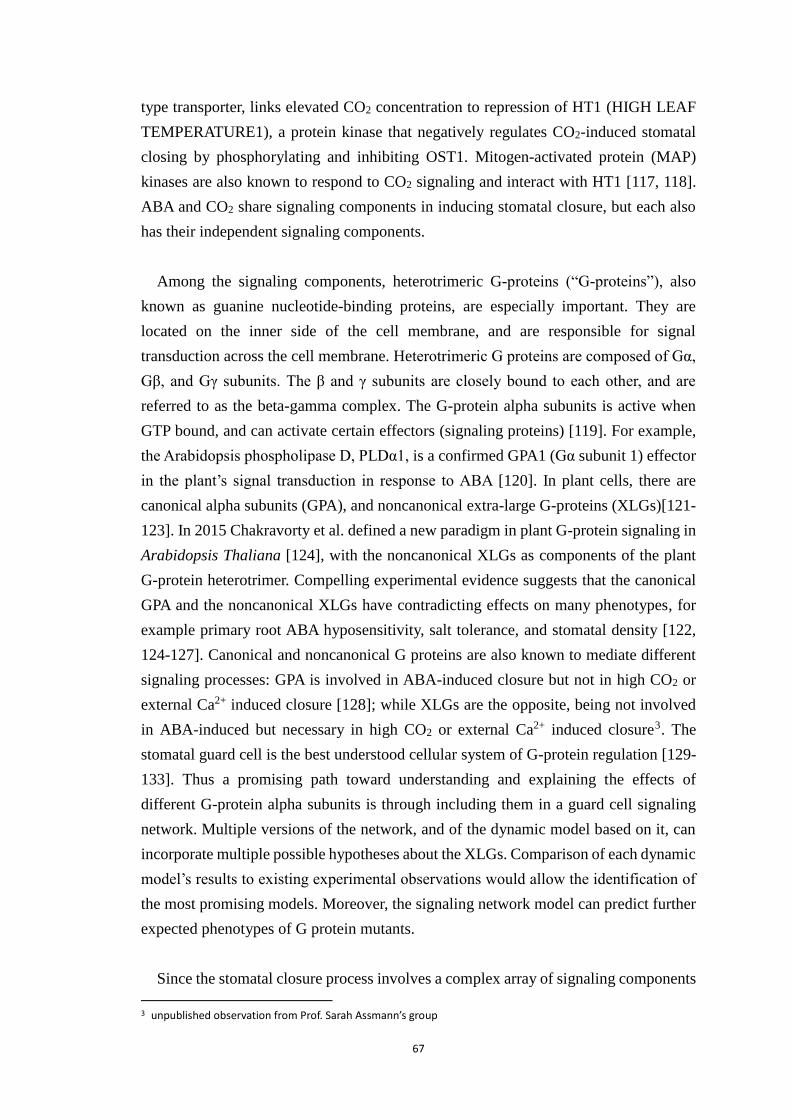
67

type transporter, links elevated CO2 concentration to repression of HT1 (HIGH LEAF

TEMPERATURE1), a protein kinase that negatively regulates CO2-induced stomatal

closing by phosphorylating and inhibiting OST1. Mitogen-activated protein (MAP)

kinases are also known to respond to CO2 signaling and interact with HT1 [117, 118].

ABA and CO2 share signaling components in inducing stomatal closure, but each also

has their independent signaling components.

Among the signaling components, heterotrimeric G-proteins (“G-proteins”), also

known as guanine nucleotide-binding proteins, are especially important. They are

located on the inner side of the cell membrane, and are responsible for signal

transduction across the cell membrane. Heterotrimeric G proteins are composed of Gα,

Gβ, and Gγ subunits. The β and γ subunits are closely bound to each other, and are

referred to as the beta-gamma complex. The G-protein alpha subunits is active when

GTP bound, and can activate certain effectors (signaling proteins) [119]. For example,

the Arabidopsis phospholipase D, PLDα1, is a confirmed GPA1 (Gα subunit 1) effector

in the plant’s signal transduction in response to ABA [120]. In plant cells, there are

canonical alpha subunits (GPA), and noncanonical extra-large G-proteins (XLGs)[121-

123]. In 2015 Chakravorty et al. defined a new paradigm in plant G-protein signaling in

Arabidopsis Thaliana [124], with the noncanonical XLGs as components of the plant

G-protein heterotrimer. Compelling experimental evidence suggests that the canonical

GPA and the noncanonical XLGs have contradicting effects on many phenotypes, for

example primary root ABA hyposensitivity, salt tolerance, and stomatal density [122,

124-127]. Canonical and noncanonical G proteins are also known to mediate different

signaling processes: GPA is involved in ABA-induced closure but not in high CO2 or

external Ca2+ induced closure [128]; while XLGs are the opposite, being not involved

in ABA-induced but necessary in high CO2 or external Ca2+ induced closure3. The

stomatal guard cell is the best understood cellular system of G-protein regulation [129-

133]. Thus a promising path toward understanding and explaining the effects of

different G-protein alpha subunits is through including them in a guard cell signaling

network. Multiple versions of the network, and of the dynamic model based on it, can

incorporate multiple possible hypotheses about the XLGs. Comparison of each dynamic

model’s results to existing experimental observations would allow the identification of

the most promising models. Moreover, the signaling network model can predict further

expected phenotypes of G protein mutants.

Since the stomatal closure process involves a complex array of signaling components

3 unpublished observation from Prof. Sarah Assmann’s group

68

and their interactions in guard cells, network-based modeling is an ideal approach to

study the guard cell signal transduction system. A network reflects signal transduction

by employing nodes representing the biological entities involved in the process, and

edges representing interactions and relationships. Then, a comprehensive dynamic

model built on the network, with each node associated with a state variable that changes

over time, can simulate how the system responds to a signal, and predict how

mutations/intervention would change the response. Together, network-based modeling

can explain how an ensemble of lower-level interactions, such as protein interactions or

phosphorylation, can lead to the system-level behavior like stomatal closure.

Prof. Réka Albert’s group has constructed several network models on guard cell

signaling and stomatal response to different signals. In 2006 Li et al. constructed the

first discrete model of the ABA signaling network that mediates stomatal closure [46].

The model successfully reproduced many observed knockout phenotypes, and predicted

new mutant response to ABA. A new, updated version of the same ABA signaling

process, published in 2017 [134] expanded the knowledge by including the results of

studies published since 2006, identified key feedback loops that can sustain their activity

in presence or absence of ABA, and made new predictions. In another work (reviewed

in Chapter 1 and 2), Sun et al. constructed a multi-level discrete model reflecting the

stomata opening process, in response to light of different wavelength, CO2, and abscisic

acid [1]. The model predicted ABA inhibition on red-light induced stomatal opening,

and the prediction is verified experimentally. These previous works provide a solid

background for a crosstalk model involving multiple signals.

While there has been intensive past work on ABA signaling network, little has been

done on a system level on CO2 signaling. Especially, no work has considered the

crosstalk between the two signals in inducing stomatal closure from a comprehensive

system-level perspective. With the new evidence that different G-protein subunits have

different effects on different signals, it would be natural to try to establish a

comprehensive crosstalk model to explain all the experimental observations. In this

work we constructed a new predictive model of the early stages of ABA/CO2 signaling

in guard cells, focusing on the crosstalk of the two signals and the effect of different G-

protein alpha subunits. The ABA part of the network is based on the ABA model by

Albert et al [134]. We used a novel method to analyze the dynamic repertoire of the

model, to identify key feedback loops that govern the model’s dynamic behavior, and

to explain the mechanism of the closure response to different signals. We predict several

new regulations in the ABA-CO2 crosstalk, potential experiments to validate these

predictions, and closure response of mutants in presence of treatments.

69

Construction and simulation methods of the crosstalk network and dynamic model

We constructed the network model based on simplification of the ABA model

proposed in 2017 [134] (which will be referred to as the “ABA model”. We start with

the strongly-connected component (SCC) of the ABA model and add CO2 related nodes.

We apply dynamics-preserving reduction methods to the SCC to reduce its size without

changing its dynamic repertoire [13, 14], so the resulting reduced SCC has the same

long-time behavior (attractors) compared with the original. In the ABA model the in-

component (upstream) of the SCC contained many input nodes that represent e.g. cell

environment. These nodes does not change state during ABA signaling, so can we

reduce them by plugging their state directly into the nodes they regulate, without

changing the system’s attractors [13]. The out-component (downstream) of the SCC is

approximated with Aquaporin and three representative ion channel nodes. Since there

is no feedback from the downstream to the SCC, approximations like this do not change

long-time dynamic behavior of the model [3, 26], i.e. again we are simplifying the

network model without changing its attractors. As a result of these simplifications, the

network was reduced from 84 nodes and 156 edges to 28 nodes and 59 edges. This

greatly reduced the complexity of the network, allowing easier analysis. To construct

the CO2 signaling pathway, we examined known signaling components and their

regulations, and add them as additional node and edges such that the network model

simulations are consistent with experimental observations. Details of the construction

process are described in the next section. Figure 4.1 shows the ABA-CO2 crosstalk

network. Similar to the ABA model, the crosstalk model has a single large SCC (18

nodes) containing early guard cell signaling components. Red edges are predicted so the

model can reproduce known closure responses (see the next section for details).

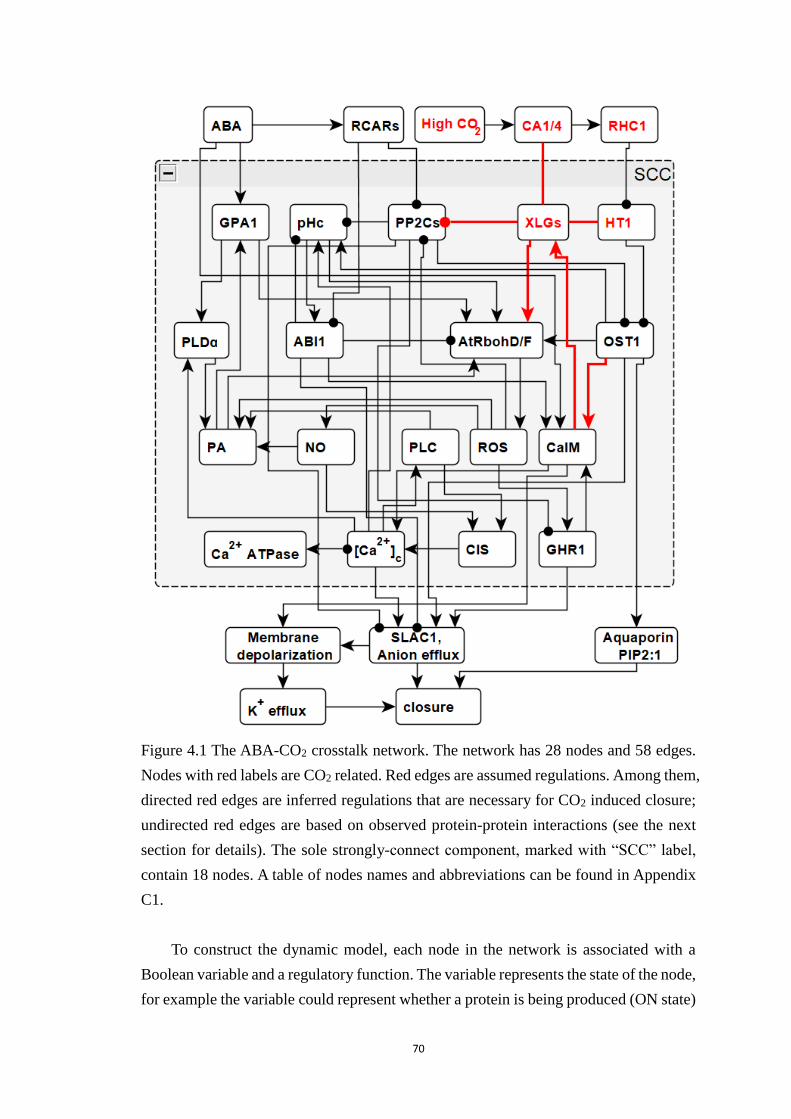
70

Figure 4.1 The ABA-CO2 crosstalk network. The network has 28 nodes and 58 edges.

Nodes with red labels are CO2 related. Red edges are assumed regulations. Among them,

directed red edges are inferred regulations that are necessary for CO2 induced closure;

undirected red edges are based on observed protein-protein interactions (see the next

section for details). The sole strongly-connect component, marked with “SCC” label,

contain 18 nodes. A table of nodes names and abbreviations can be found in Appendix

C1.

To construct the dynamic model, each node in the network is associated with a

Boolean variable and a regulatory function. The variable represents the state of the node,

for example the variable could represent whether a protein is being produced (ON state)

71

or not (OFF state), or represent the concentration level of a molecule (ON for high

concentration, OFF for low concentration). The regulatory function describes how the

node variable changes over time. Specifically, we employ a discrete time framework, so

the regulatory functions determine the node variable at the next time step. For the

dynamic system, we apply a random-order asynchronous update: at each time step, all

nodes in the network are updated in a random order. Introducing stochasticity here is a

good method to make up for the lack timing details of the regulations. If one tracks a

node variable over time, one can get a single time-course simulation, representing how

the node behaves over time within one simulation. We perform a large ensemble of time-

course simulations (e.g. 1000 simulations) and average their data. The simulations are

performed from a partially fixed initial system state, where the states of signal

components are set to their observed values in reality. For the a few nodes whose initial

state we do not know, their initial states are randomized. In this model, the only

randomly-initialized nodes are SLAC1 Anion Channel, Membrane depolarization, K+

efflux, and Aquaporin PIP2:1.

Figure 4.2 shows representative simulations as wild type stomatal closure response

to different signals ABA, CO2, and external Calcium. Monte-Carlo simulation allows

the generation of time course data (i.e. the time a variable converges to its attractor state)

and enables quantitative analysis on a Boolean model, under the stochastic update

scheme. If the simulated value reaches and stays at 0 or 1 after long enough, then we

know the node converges to a stabilized value 0 or 1 in all the simulations, suggesting

a sole attractor with this node in a fixed value. If the final value is in between 0 and 1,

there may be multi-stability or a complex attractor. A fluctuation of the node value is

the signature of a complex attractor; while a stabilized node value (between 0 and 1)

implies multistability of steady states.

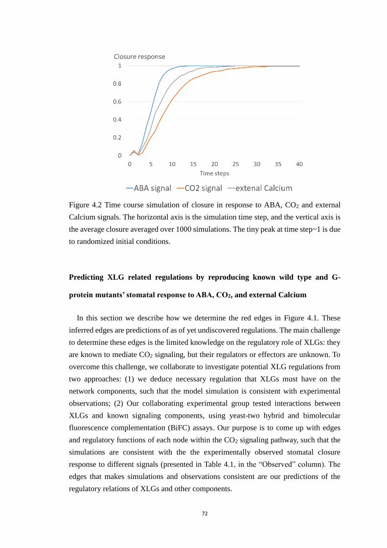
72

Figure 4.2 Time course simulation of closure in response to ABA, CO2 and external

Calcium signals. The horizontal axis is the simulation time step, and the vertical axis is

the average closure averaged over 1000 simulations. The tiny peak at time step~1 is due

to randomized initial conditions.

Predicting XLG related regulations by reproducing known wild type and G-

protein mutants’ stomatal response to ABA, CO2, and external Calcium

In this section we describe how we determine the red edges in Figure 4.1. These

inferred edges are predictions of as of yet undiscovered regulations. The main challenge

to determine these edges is the limited knowledge on the regulatory role of XLGs: they

are known to mediate CO2 signaling, but their regulators or effectors are unknown. To

overcome this challenge, we collaborate to investigate potential XLG regulations from

two approaches: (1) we deduce necessary regulation that XLGs must have on the

network components, such that the model simulation is consistent with experimental

observations; (2) Our collaborating experimental group tested interactions between

XLGs and known signaling components, using yeast-two hybrid and bimolecular

fluorescence complementation (BiFC) assays. Our purpose is to come up with edges

and regulatory functions of each node within the CO2 signaling pathway, such that the

simulations are consistent with the the experimentally observed stomatal closure

response to different signals (presented in Table 4.1, in the “Observed” column). The

edges that makes simulations and observations consistent are our predictions of the

regulatory relations of XLGs and other components.

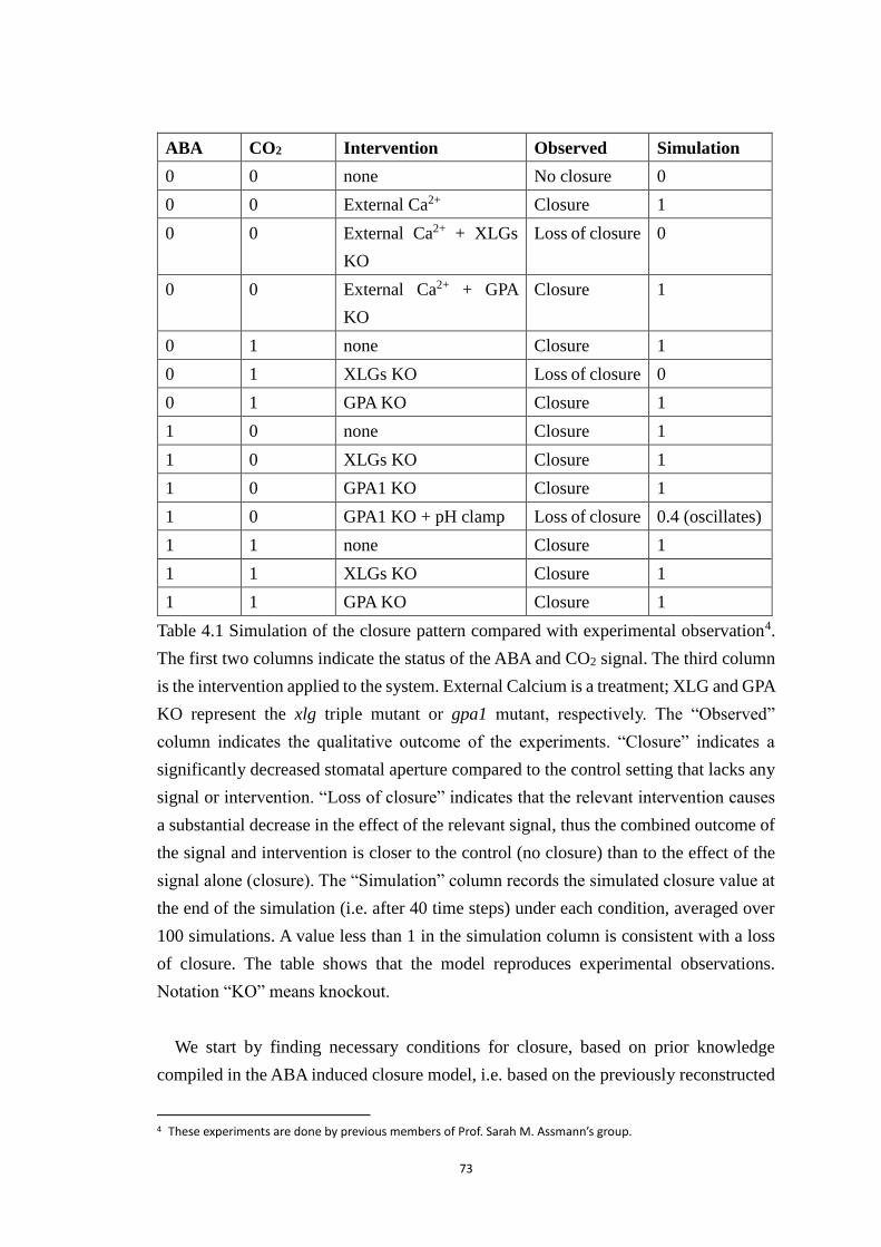
73

ABA CO2 Intervention Observed Simulation

0 0 none No closure 0

0 0 External Ca2+ Closure 1

0 0 External Ca2+ + XLGs

KO

Loss of closure 0

0 0 External Ca2+ + GPA

KO

Closure 1

0 1 none Closure 1

0 1 XLGs KO Loss of closure 0

0 1 GPA KO Closure 1

1 0 none Closure 1

1 0 XLGs KO Closure 1

1 0 GPA1 KO Closure 1

1 0 GPA1 KO + pH clamp Loss of closure 0.4 (oscillates)

1 1 none Closure 1

1 1 XLGs KO Closure 1

1 1 GPA KO Closure 1

Table 4.1 Simulation of the closure pattern compared with experimental observation4.

The first two columns indicate the status of the ABA and CO2 signal. The third column

is the intervention applied to the system. External Calcium is a treatment; XLG and GPA

KO represent the xlg triple mutant or gpa1 mutant, respectively. The “Observed”

column indicates the qualitative outcome of the experiments. “Closure” indicates a

significantly decreased stomatal aperture compared to the control setting that lacks any

signal or intervention. “Loss of closure” indicates that the relevant intervention causes

a substantial decrease in the effect of the relevant signal, thus the combined outcome of

the signal and intervention is closer to the control (no closure) than to the effect of the

signal alone (closure). The “Simulation” column records the simulated closure value at

the end of the simulation (i.e. after 40 time steps) under each condition, averaged over

100 simulations. A value less than 1 in the simulation column is consistent with a loss

of closure. The table shows that the model reproduces experimental observations.

Notation “KO” means knockout.

We start by finding necessary conditions for closure, based on prior knowledge

compiled in the ABA induced closure model, i.e. based on the previously reconstructed

4 These experiments are done by previous members of Prof. Sarah M. Assmann’s group.

74

regulatory functions of the nodes in the ABA pathway. We identified three necessary

conditions for closure in the absence of ABA: inhibition of the PP2C protein

phosphatases (which otherwise would inhibit closure), activation of AtRbohD/F (in

order to produce reactive oxygen species ROS, a type of secondary messengers

necessary for multiple processes), and CaIM (Ca2+ influx through the membrane, which

is the first process that can yield the Ca2+c increase). These conditions must be met in

CO2 signaling, because CO2 can induce stomatal closure in the absence of ABA. Each

necessary condition is translated into a regulatory edge, through which CO2 signaling

can meet the condition. These edges are the directed red edges in Figure 4.1. In the

following part, we list these edges, with an explanation why each edge is necessary, and

point out potential experiments that can help validate them.

1. XLGs -| PP2C inhibitory regulation

PP2Cs inhibit OST1 and are inhibited by ABA receptors in ABA signaling. Under

CO2 signaling the ABA receptors are inactive but PP2Cs still need to be inhibited to

obtain closure. We assume that XLGs are responsible for this inhibition, either directly

or indirectly. Our collaborators have found evidence of XLGs (XLG3 specifically),

interaction with some of the PP2Cs (ABI2 and HAB1) in both yeast-two hybrid assays

and BiFC assays. Experiments showing XLG activity causing decreased PP2C

phosphatase activity, or experiments showing XLG activation associated with low PP2C

activity under high CO2 would be a good validation of this assumption.

2. XLGs AtRbohD/F regulation

AtRbohD/F enzymes catalyze ROS production in guard cells, which is essential for

ABA-induced stomatal closure. It is also reported that ROS production is necessary in

CO2 signaling [135]. Under ABA, AtrbohD/F is activated by GPA1, which is not

necessary in CO2 signaling. Therefore, under CO2 signaling, some other signaling

component should be able to take GPA1’s place and activate AtRbohD/F. We assume

XLGs are responsible for the activation of AtRbohD/F under CO2 signaling. Our

collaborators have found evidence of XLG interaction with AtRbohD in yeast-two

hybrid assay and BiFC assay. Observation of (1) loss of ROS production in xlg triple

mutants under CO2 signal; or (2) ROS treatment being able to restore xlg mutants’ loss

of closure in response to CO2 would further validate this regulation.

3. CaIM XLGs regulation

XLG is necessary for external Calcium induced closure. The simplest way to

implement this is to assume that XLG is activated by external Calcium and it mediates

75

its closure-inducing effects. Since external Calcium is represented in the model as CaIM

(Calcium influx through membrane) being constitutively ON, we decide to add a CaIM

XLGs regulation edge.

4. OST1 CaIM regulation

CaIM is necessary to induce an initial increase of the cytosolic Ca2+ (denoted Ca2+c ).

The Ca2+c level cannot stay elevated for long due to its toxic effects to cells [136, 137];

instead, repeated peaks of Ca2+c are observed, and were proposed to be necessary for the

closure process[138]. CaIM can be activated by many nodes in the ABA model.

However most of its activators can only activate CaIM after an initial CaIM activation.

It works like an engine that needs a CaIM “ignition” process, after which it can sustain

itself. The “ignition” of CaIM under ABA signaling is provided by an independent

stretch-activated channel mechanism activated by actin reorganization [110], which is

not activated in CO2 signaling. Therefore CO2 has to induce initial CaIM activation

through a different regulation mechanism. We assume OST1 is responsible for the

ignition of CaIM under CO2, and add an edge OST1 CaIM. We did not assume XLGs

as responsible for this, because after we assumed CaIM XLG, adding XLG CaIM

feedback could result in a partial fixed point where XLGs and CaIM remain inactivated

regardless of the other nodes.

The experimental results of our collaborators help construct the rest of the network.

Four interactions, namely CA1/4 – XLGs, XLGs - HT1, XLGs – AtRbohD/F, and XLGs

– PP2Cs interactions, were found experimentally. Among them, XLGs – AtRbohD/F

and XLGs – PP2Cs interactions are already assumed in the previous approach; this

experimental evidence helps validate those assumptions. The other two interactions,

CA1/4 – XLGs and XLGs - HT1 interactions, are tested in simulations to see if they can

make simulations consistent with experimental observations. Since the protein-protein

interaction experimental assays only suggests physical interaction (binding) but not

regulation (i.e. an interaction does not guarantee a regulatory effect, and does not

indicate which interacting partner is the regulator and which the target), we have to test

all possible settings of the two edges, by testing their direction and whether they can be

removed without causing inconsistency. In principle we have to test the sign of the two

edges too, i.e. whether the regulation is positive (promoting) or negative (inhibitory).

To simplify, we assumed the sign of the edge according to the regulatory role of the

nodes. That is, we assume an edge between two up-regulators or two down-regulators

of closure (i.e. CA1/4 - XLGs) to be positive, and assume an edge between an up-

regulator and a down-regulator (i.e. XLGs – HT1) to be negative. With this assumption,

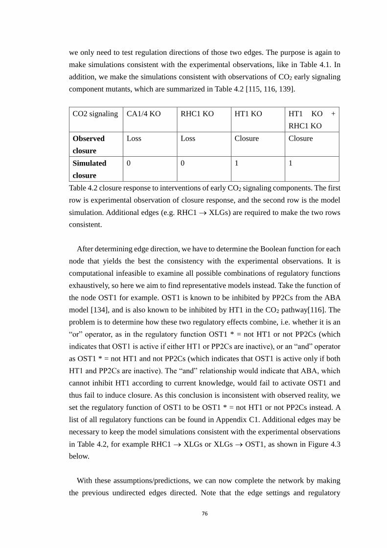
76

we only need to test regulation directions of those two edges. The purpose is again to

make simulations consistent with the experimental observations, like in Table 4.1. In

addition, we make the simulations consistent with observations of CO2 early signaling

component mutants, which are summarized in Table 4.2 [115, 116, 139].

CO2 signaling CA1/4 KO RHC1 KO HT1 KO HT1 KO +

RHC1 KO

Observed

closure

Loss Loss Closure Closure

Simulated

closure

0 0 1 1

Table 4.2 closure response to interventions of early CO2 signaling components. The first

row is experimental observation of closure response, and the second row is the model

simulation. Additional edges (e.g. RHC1 XLGs) are required to make the two rows

consistent.

After determining edge direction, we have to determine the Boolean function for each

node that yields the best the consistency with the experimental observations. It is

computational infeasible to examine all possible combinations of regulatory functions

exhaustively, so here we aim to find representative models instead. Take the function of

the node OST1 for example. OST1 is known to be inhibited by PP2Cs from the ABA

model [134], and is also known to be inhibited by HT1 in the CO2 pathway[116]. The

problem is to determine how these two regulatory effects combine, i.e. whether it is an

“or” operator, as in the regulatory function OST1 * = not HT1 or not PP2Cs (which

indicates that OST1 is active if either HT1 or PP2Cs are inactive), or an “and” operator

as OST1 * = not HT1 and not PP2Cs (which indicates that OST1 is active only if both

HT1 and PP2Cs are inactive). The “and” relationship would indicate that ABA, which

cannot inhibit HT1 according to current knowledge, would fail to activate OST1 and

thus fail to induce closure. As this conclusion is inconsistent with observed reality, we

set the regulatory function of OST1 to be OST1 * = not HT1 or not PP2Cs instead. A

list of all regulatory functions can be found in Appendix C1. Additional edges may be

necessary to keep the model simulations consistent with the experimental observations

in Table 4.2, for example RHC1 XLGs or XLGs OST1, as shown in Figure 4.3

below.

With these assumptions/predictions, we can now complete the network by making

the previous undirected edges directed. Note that the edge settings and regulatory

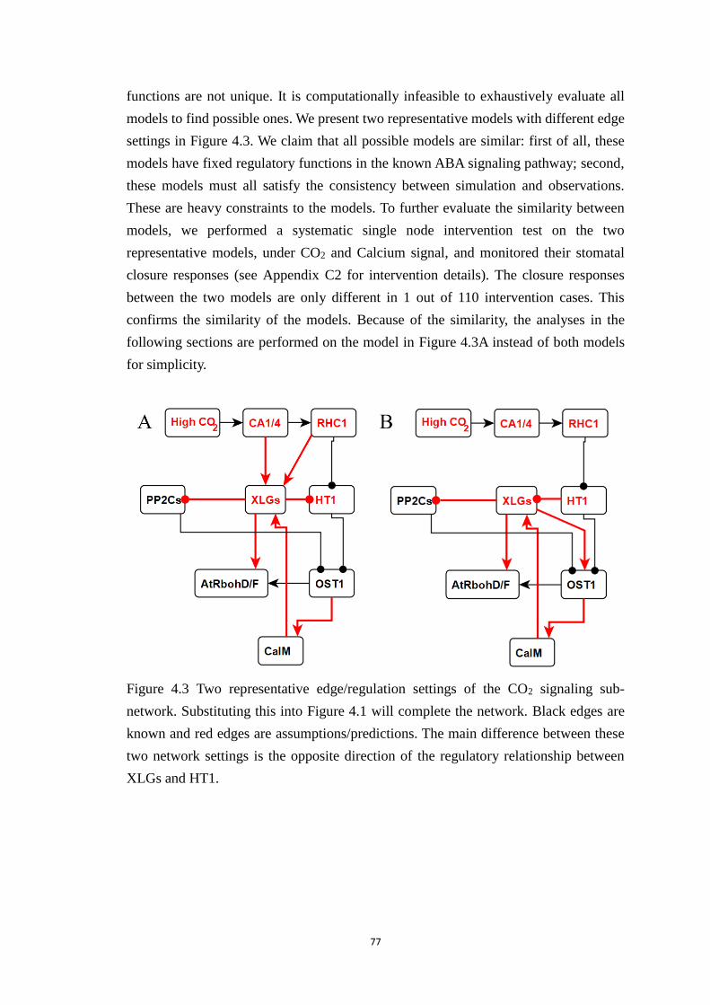
77

functions are not unique. It is computationally infeasible to exhaustively evaluate all

models to find possible ones. We present two representative models with different edge

settings in Figure 4.3. We claim that all possible models are similar: first of all, these

models have fixed regulatory functions in the known ABA signaling pathway; second,

these models must all satisfy the consistency between simulation and observations.

These are heavy constraints to the models. To further evaluate the similarity between

models, we performed a systematic single node intervention test on the two

representative models, under CO2 and Calcium signal, and monitored their stomatal

closure responses (see Appendix C2 for intervention details). The closure responses

between the two models are only different in 1 out of 110 intervention cases. This

confirms the similarity of the models. Because of the similarity, the analyses in the

following sections are performed on the model in Figure 4.3A instead of both models

for simplicity.

Figure 4.3 Two representative edge/regulation settings of the CO2 signaling sub-

network. Substituting this into Figure 4.1 will complete the network. Black edges are

known and red edges are assumptions/predictions. The main difference between these

two network settings is the opposite direction of the regulatory relationship between

XLGs and HT1.

78

Motifs analysis identifies key feedback loops, shows the attractor of the system,

and explain the effect of different G-protein alpha subunits

One of the most important features of a dynamic model is its repertoire of attractors,

which are long-time behavior of the system. Attractors usually represent biological

phenotypes, making them particularly interesting. For example, a cellular regulatory

network can have two attractors, one representing a healthy cell state, while the other

representing a cancer cell state. There are steady state attractors, where the entire system

stays in equilibrium; there are also complex/oscillatory attractors, where a subset of the

system is oscillating. Simulations of the crosstalk model showed attractors with stomatal

closure, attractors with no closure, and attractors with oscillating closure value. Note

that simulations indicate specific dynamic trajectories and cannot reveal the entire

repertoire of a dynamical system. In addition, oscillation of certain node states is

observed, indicating complex attractor. All these suggest that it is interesting to analyze

the attractors of the crosstalk model. However, it is difficult to find all attractors of a

discrete dynamical system. The only way to accurately find all attractors is to search the

state space exhaustively, which fails quickly as the state space of a discrete system scales

up exponentially.

In a previous work (described in Chapter 3), we developed a general method to find

attractors of a discrete dynamic system [33]. The method finds self-sufficient motifs

from an expanded network representation that are similar to points of no return in the

dynamics: if the system is in a state specified by such a motif, it cannot leave the motif.

One can then plug in the states specified by the motifs to reduce the network, and do

this iteratively until the whole system attractor is found. The motifs method is general

and can apply to a wide range of modeling frameworks, from Boolean to continuous

[30, 140].

We apply the motifs method to the crosstalk model to find its attractors. The results

are shown in Figure 4.4. We found a sole stable motif in the presence of a single signal,

i.e. either ABA or CO2, as shown in Figure 4.4A&B. Single stable motif means sole

attractor, which implies that closure will occur regardless of the initial condition of the

system, indicating closure as a robust process. Figure 4.4C shows the motifs found

under no signal (i.e. both ABA and CO2 being OFF). We observe bi-stability, the co-

existence of two attractors, one of which is associated with the lack of closure (i.e.

Closure=0), while the other is associated with closure. The dotted line in the closure ON

stable motif means that either XLG or GPA1 is sufficient to complete the motif. This is

interesting because a mutation or external intervention can drive the system to one

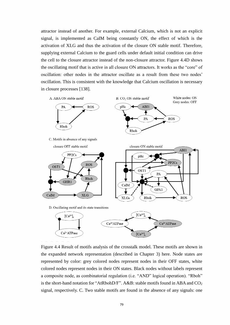
79

attractor instead of another. For example, external Calcium, which is not an explicit

signal, is implemented as CaIM being constantly ON, the effect of which is the

activation of XLG and thus the activation of the closure ON stable motif. Therefore,

supplying external Calcium to the guard cells under default initial condition can drive

the cell to the closure attractor instead of the non-closure attractor. Figure 4.4D shows

the oscillating motif that is active in all closure ON attractors. It works as the “core” of

oscillation: other nodes in the attractor oscillate as a result from these two nodes’

oscillation. This is consistent with the knowledge that Calcium oscillation is necessary

in closure processes [138].

Figure 4.4 Result of motifs analysis of the crosstalk model. These motifs are shown in

the expanded network representation (described in Chapter 3) here. Node states are

represented by color: grey colored nodes represent nodes in their OFF states, white

colored nodes represent nodes in their ON states. Black nodes without labels represent

a composite node, as combinatorial regulation (i.e. “AND” logical operation). “Rboh”

is the short-hand notation for “AtRbohD/F”. A&B: stable motifs found in ABA and CO2

signal, respectively. C. Two stable motifs are found in the absence of any signals: one

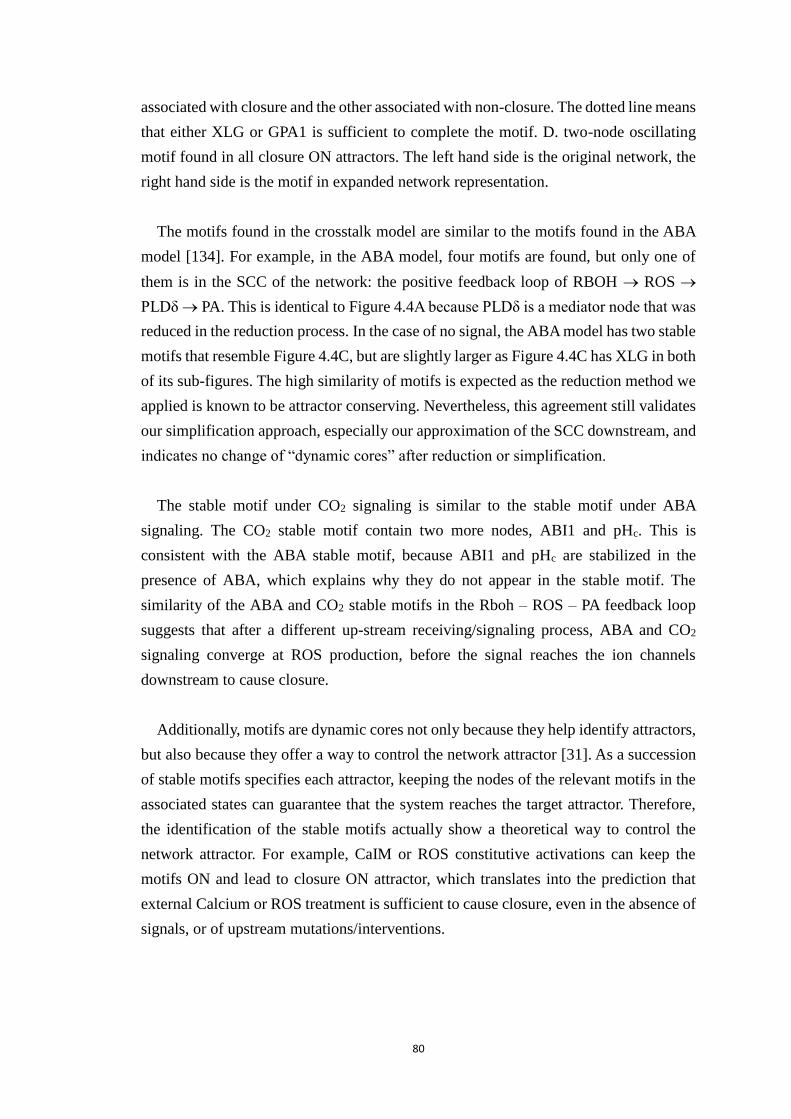
80

associated with closure and the other associated with non-closure. The dotted line means

that either XLG or GPA1 is sufficient to complete the motif. D. two-node oscillating

motif found in all closure ON attractors. The left hand side is the original network, the

right hand side is the motif in expanded network representation.

The motifs found in the crosstalk model are similar to the motifs found in the ABA

model [134]. For example, in the ABA model, four motifs are found, but only one of

them is in the SCC of the network: the positive feedback loop of RBOH ROS

PLDδ PA. This is identical to Figure 4.4A because PLDδ is a mediator node that was

reduced in the reduction process. In the case of no signal, the ABA model has two stable

motifs that resemble Figure 4.4C, but are slightly larger as Figure 4.4C has XLG in both

of its sub-figures. The high similarity of motifs is expected as the reduction method we

applied is known to be attractor conserving. Nevertheless, this agreement still validates

our simplification approach, especially our approximation of the SCC downstream, and

indicates no change of “dynamic cores” after reduction or simplification.

The stable motif under CO2 signaling is similar to the stable motif under ABA

signaling. The CO2 stable motif contain two more nodes, ABI1 and pHc. This is

consistent with the ABA stable motif, because ABI1 and pHc are stabilized in the

presence of ABA, which explains why they do not appear in the stable motif. The

similarity of the ABA and CO2 stable motifs in the Rboh – ROS – PA feedback loop

suggests that after a different up-stream receiving/signaling process, ABA and CO2

signaling converge at ROS production, before the signal reaches the ion channels

downstream to cause closure.

Additionally, motifs are dynamic cores not only because they help identify attractors,

but also because they offer a way to control the network attractor [31]. As a succession

of stable motifs specifies each attractor, keeping the nodes of the relevant motifs in the

associated states can guarantee that the system reaches the target attractor. Therefore,

the identification of the stable motifs actually show a theoretical way to control the

network attractor. For example, CaIM or ROS constitutive activations can keep the

motifs ON and lead to closure ON attractor, which translates into the prediction that

external Calcium or ROS treatment is sufficient to cause closure, even in the absence of

signals, or of upstream mutations/interventions.

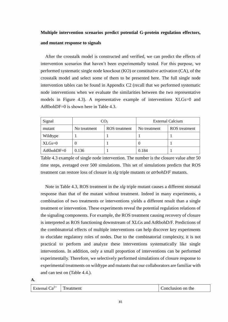
81

Multiple intervention scenarios predict potential G-protein regulation effectors,

and mutant response to signals

After the crosstalk model is constructed and verified, we can predict the effects of

intervention scenarios that haven’t been experimentally tested. For this purpose, we

performed systematic single node knockout (KO) or constitutive activation (CA), of the

crosstalk model and select some of them to be presented here. The full single node

intervention tables can be found in Appendix C2 (recall that we performed systematic

node interventions when we evaluate the similarities between the two representative

models in Figure 4.3). A representative example of interventions XLGs=0 and

AtRbohDF=0 is shown here in Table 4.3.

Signal CO2 External Calcium

mutant No treatment ROS treatment No treatment ROS treatment

Wildtype 1 1 1 1

XLGs=0 0 1 0 1

AtRbohDF=0 0.136 1 0.184 1

Table 4.3 example of single node intervention. The number is the closure value after 50

time steps, averaged over 500 simulations. This set of simulations predicts that ROS

treatment can restore loss of closure in xlg triple mutants or atrbohD/F mutants.

Note in Table 4.3, ROS treatment in the xlg triple mutant causes a different stomatal

response than that of the mutant without treatment. Indeed in many experiments, a

combination of two treatments or interventions yields a different result than a single

treatment or intervention. These experiments reveal the potential regulation relations of

the signaling components. For example, the ROS treatment causing recovery of closure

is interpreted as ROS functioning downstream of XLGs and AtRbohD/F. Predictions of

the combinatorial effects of multiple interventions can help discover key experiments

to elucidate regulatory roles of nodes. Due to the combinatorial complexity, it is not

practical to perform and analyze these interventions systematically like single

interventions. In addition, only a small proportion of interventions can be performed

experimentally. Therefore, we selectively performed simulations of closure response to

experimental treatments on wildtype and mutants that our collaborators are familiar with

and can test on (Table 4.4.).

A.

External Ca2+ Treatment Conclusion on the

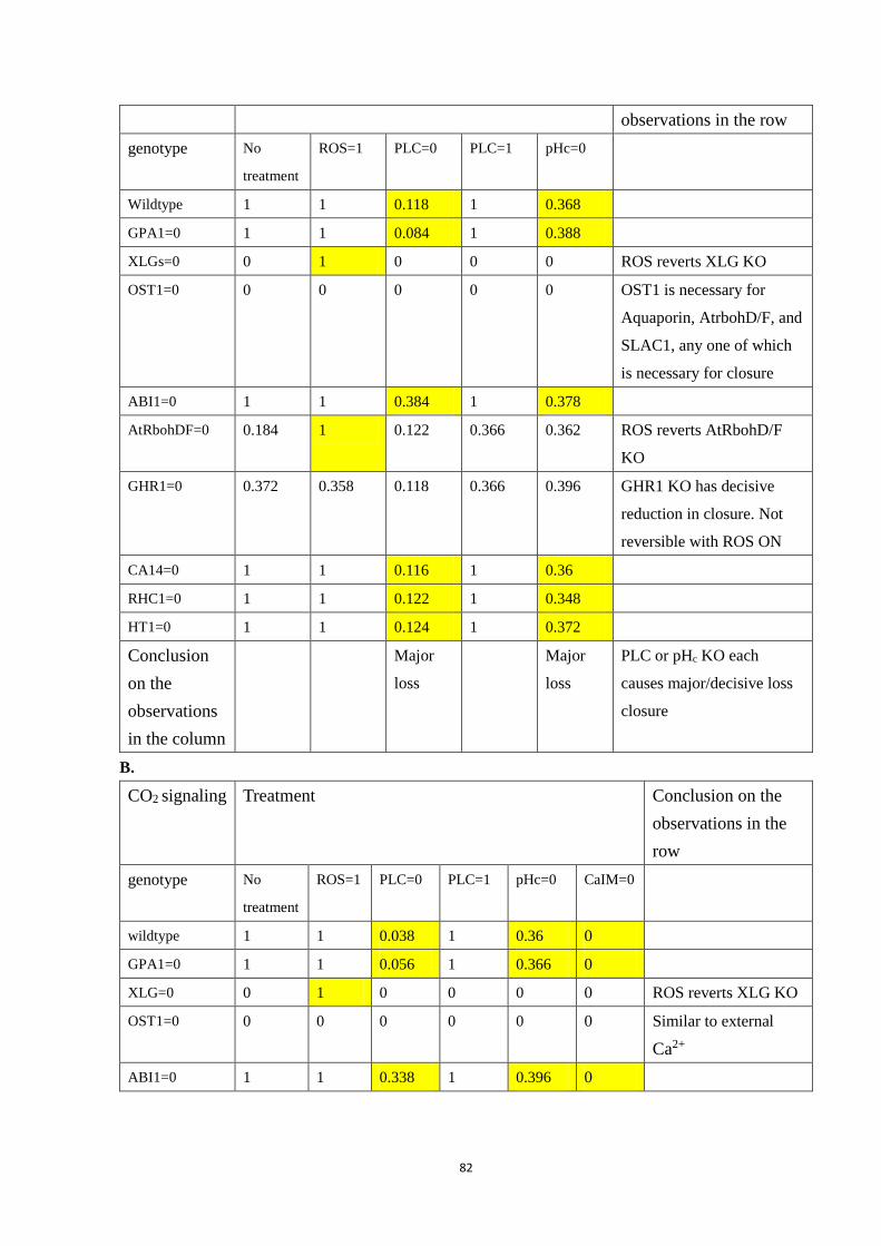
82

observations in the row

genotype No

treatment

ROS=1 PLC=0 PLC=1 pHc=0

Wildtype 1 1 0.118 1 0.368

GPA1=0 1 1 0.084 1 0.388

XLGs=0 0 1 0 0 0 ROS reverts XLG KO

OST1=0 0 0 0 0 0 OST1 is necessary for

Aquaporin, AtrbohD/F, and

SLAC1, any one of which

is necessary for closure

ABI1=0 1 1 0.384 1 0.378

AtRbohDF=0 0.184 1 0.122 0.366 0.362 ROS reverts AtRbohD/F

KO

GHR1=0 0.372 0.358 0.118 0.366 0.396 GHR1 KO has decisive

reduction in closure. Not

reversible with ROS ON

CA14=0 1 1 0.116 1 0.36

RHC1=0 1 1 0.122 1 0.348

HT1=0 1 1 0.124 1 0.372

Conclusion

on the

observations

in the column

Major

loss

Major

loss

PLC or pHc KO each

causes major/decisive loss

closure

B.

CO2 signaling Treatment Conclusion on the

observations in the

row

genotype No

treatment

ROS=1 PLC=0 PLC=1 pHc=0 CaIM=0

wildtype 1 1 0.038 1 0.36 0

GPA1=0 1 1 0.056 1 0.366 0

XLG=0 0 1 0 0 0 0 ROS reverts XLG KO

OST1=0 0 0 0 0 0 0 Similar to external

Ca2+

ABI1=0 1 1 0.338 1 0.396 0

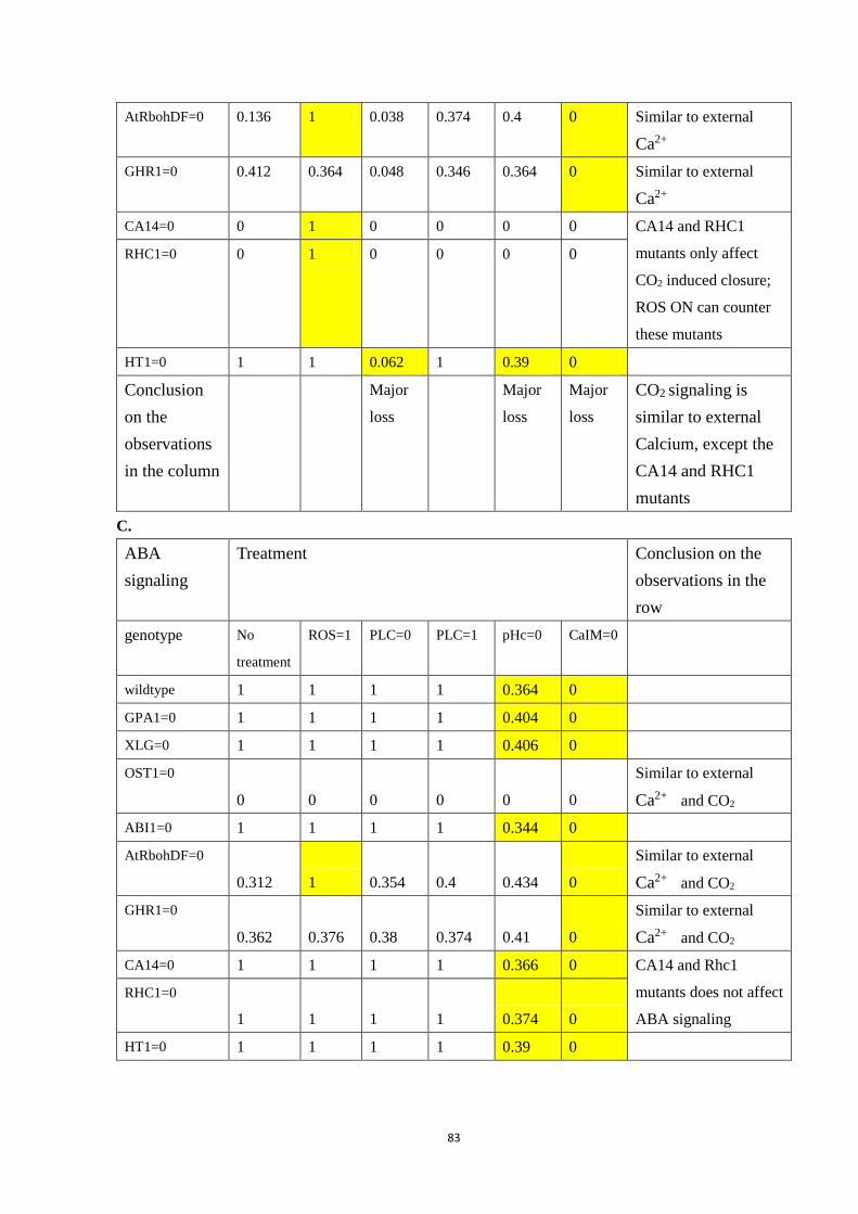
83

AtRbohDF=0 0.136 1 0.038 0.374 0.4 0 Similar to external

Ca2+

GHR1=0 0.412 0.364 0.048 0.346 0.364 0 Similar to external

Ca2+

CA14=0 0 1 0 0 0 0 CA14 and RHC1

mutants only affect

CO2 induced closure;

ROS ON can counter

these mutants

RHC1=0 0 1 0 0 0 0

HT1=0 1 1 0.062 1 0.39 0

Conclusion

on the

observations

in the column

Major

loss

Major

loss

Major

loss

CO2 signaling is

similar to external

Calcium, except the

CA14 and RHC1

mutants

C.

ABA

signaling

Treatment Conclusion on the

observations in the

row

genotype No

treatment

ROS=1 PLC=0 PLC=1 pHc=0 CaIM=0

wildtype 1 1 1 1 0.364 0

GPA1=0 1 1 1 1 0.404 0

XLG=0 1 1 1 1 0.406 0

OST1=0

0 0 0 0 0 0

Similar to external

Ca2+ and CO2

ABI1=0 1 1 1 1 0.344 0

AtRbohDF=0

0.312 1 0.354 0.4 0.434 0

Similar to external

Ca2+ and CO2

GHR1=0

0.362 0.376 0.38 0.374 0.41 0

Similar to external

Ca2+ and CO2

CA14=0 1 1 1 1 0.366 0 CA14 and Rhc1

mutants does not affect

ABA signaling

RHC1=0

1 1 1 1 0.374 0

HT1=0 1 1 1 1 0.39 0

84

Conclusion

on the

observations

in the column

No loss Major

loss

Major

loss

ABA signaling does

not depend of PLC

Table 4.4 Selected double interventions under each signal: A. External Ca2+; B. CO2; C.

ABA. Each row is a genotype (wildtype or the indicated mutant), and each column is a

treatment (including no special treatment). All simulated closure values are reported

after 50 time steps, averaged over 500 simulations. Yellowed slots are those that display

a significantly different value compared with no treatment. Conclusion on the

observations in the row/column are located on the last column/row of each sub-table.

Table 4.4 reveals interesting results: (1) CA14 and RHC1 mutants do not affect

external Ca2+ or ABA signaling. This is expected as CA1/4 and RHC1 are CO2 early

components and are not part of the network’s SCC. (2) ROS treatment can revert closure

loss caused by XLG KO or by AtRbohD/F KO. (3) pHc KO causes loss of closure for

all signals, all mutants. (4) CaIM KO causes loss of closure for all signals, all mutants.

(5) PLC treatment has a different effect under ABA signaling (no loss) than the other

two signals (loss of closure). (6) OST1 KO mutant causes loss of closure and cannot be

recovered by any treatment. (7) GHR1 KO mutant causes loss of closure and cannot be

recovered by any treatment.

To investigate further we performed triple interventions. The full simulation table can

be found in Appendix C3; here we summarize some of the interesting findings.

Examples of interesting findings include: (1) ROS =1 treatment can recover closure

from PLC=0 treatment, under all three signals. (2) ROS ON can revert closure loss due

to pHc KO treatment. (3) pHc KO can induce closure loss despite PLC ON treatment.

Note that some of the “double treatment” interventions may not be practical to perform.

The crosstalk model offers a potential explanation to the seemingly contradictory

stomatal response to CO2 in presence and absence of mesophyll cells

There has been controversy on how mesophyll cells may contribute to the regulation

on stomatal closure under CO2 signaling. Mesophyll cells are in the middle of plant

leaves, below the epidermis where the guard cells are. They have a lot of chloroplasts

in them, and are thus the main sites of photosynthesis [141]. Stomatal closure

experiments are done in different settings: on whole leaves or whole plants, where

85

mesophyll cells are present, or on epidermal peels where mesophyll cells are absent.

Different groups have reported that the stomatal aperture responses to CO2 in whole

leaves and epidermal peels are different: the closure response is much less in epidermal

peels [142, 143]. Our collaborators have also found that the xlg triple mutant retains

closure in live plants, in contrast to their loss of closure response in epidermal peels5.

Despite these observations, whether mesophyll play a significant and independent role

in stomatal closure is still debated. Assumptions of a diffusible factor known as ‘the

mesophyll signal’ that regulates stomatal movement have been expressed in the

literature for a very long time [141, 142, 144]. However, it remains unclear what this

signaling component is.

With the help of our network model, we can evaluate the hypothesis that mesophyll

cells regulate stomatal closure by adding an additional node “mesophyll signal” into the

network. In our model, mesophyll signal is assumed to be regulated by CA1/4, to

represent the fact that mesophyll cells take bicarbonate, the product of CA1/4 mediated

CO2 fixation, for photosynthesis; and to be consistent with the fact that CA1/4 mutant

lose all CO2 induced closure [115]. With the mesophyll signal unknown, we test

potential mesophyll regulation by assuming an additional edge from mesophyll to its

potential second messengers. The mesophyll signal can be mediated by products of

biosynthesis like ABA, sucrose, and apoplastic malate, or the signal can have other

effectors, like apoplastic pH or guard cell ion channels.

Our model has nodes ABA and pHc (cytosolic pH), so a straightforward approach is

to test the hypothesis that mesophyll cells produce ABA, or regulate pHc, by seeing if

the simulations can reproduce the different CO2 response of xlg mutants in whole leaf

and epidermal peel experiments. We start with the hypothesis that mesophyll cells

produce or release ABA. There is evidence in the literature that ABA is being produced

in mesophyll cells to support this hypothesis [145]. We implement this hypothesis into

the network model by adding mesophyll ABA activation edge. The resulting network

model simulations shows that xlg mutant and rhc1 mutant displays different closure

response in the absence or presence of mesophyll (Table 4.5). The simulation also shows

consistency with the knowledge that the ca1/4 mutants are insensitive to CO2 in both

epidermal peels and live plants [115]. Notably, the closure response of rhc1 mutant is

in controversy: Tian et al. reports that rhc1 mutant plants have reduced CO2 sensitivity

in live plant measurements and are insensitive to CO2 in epidermal peels[116]; while a

recent report from Tõldsepp et al. finds normal (or close to normal) sensitivity of rhc1

5 These experiments (unpublished) are done by members of Prof. Sarah M. Assmann’s group.

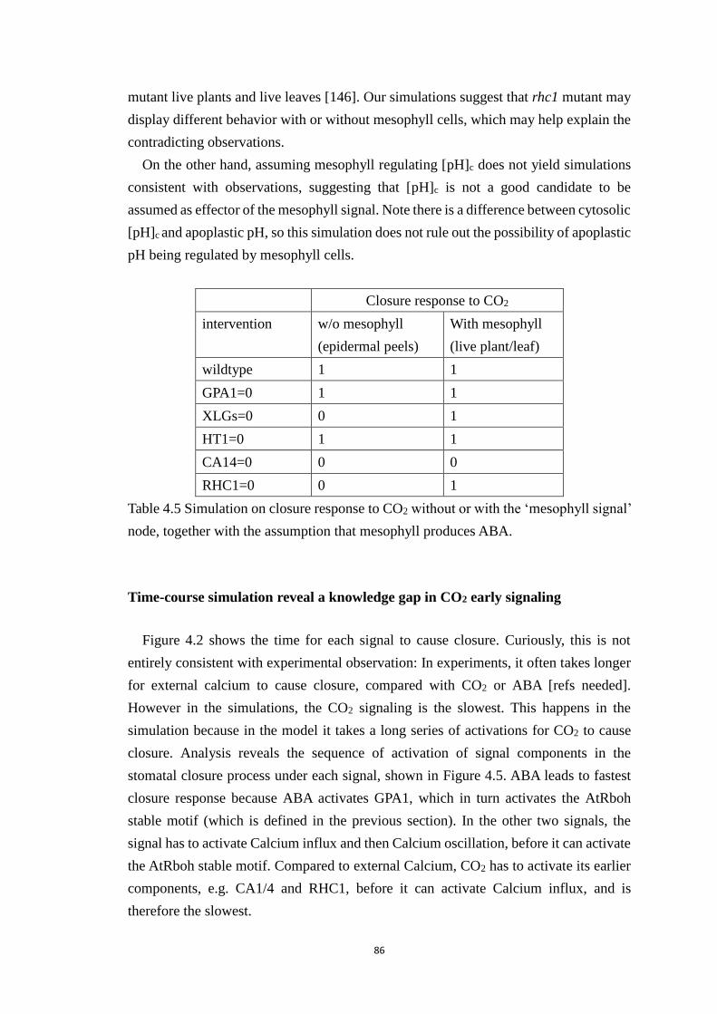
86

mutant live plants and live leaves [146]. Our simulations suggest that rhc1 mutant may

display different behavior with or without mesophyll cells, which may help explain the

contradicting observations.

On the other hand, assuming mesophyll regulating [pH]c does not yield simulations

consistent with observations, suggesting that [pH]c is not a good candidate to be

assumed as effector of the mesophyll signal. Note there is a difference between cytosolic

[pH]c and apoplastic pH, so this simulation does not rule out the possibility of apoplastic

pH being regulated by mesophyll cells.

Closure response to CO2

intervention w/o mesophyll

(epidermal peels)

With mesophyll

(live plant/leaf)

wildtype 1 1

GPA1=0 1 1

XLGs=0 0 1

HT1=0 1 1

CA14=0 0 0

RHC1=0 0 1

Table 4.5 Simulation on closure response to CO2 without or with the ‘mesophyll signal’

node, together with the assumption that mesophyll produces ABA.

Time-course simulation reveal a knowledge gap in CO2 early signaling

Figure 4.2 shows the time for each signal to cause closure. Curiously, this is not

entirely consistent with experimental observation: In experiments, it often takes longer

for external calcium to cause closure, compared with CO2 or ABA [refs needed].

However in the simulations, the CO2 signaling is the slowest. This happens in the

simulation because in the model it takes a long series of activations for CO2 to cause

closure. Analysis reveals the sequence of activation of signal components in the

stomatal closure process under each signal, shown in Figure 4.5. ABA leads to fastest

closure response because ABA activates GPA1, which in turn activates the AtRboh

stable motif (which is defined in the previous section). In the other two signals, the

signal has to activate Calcium influx and then Calcium oscillation, before it can activate

the AtRboh stable motif. Compared to external Calcium, CO2 has to activate its earlier

components, e.g. CA1/4 and RHC1, before it can activate Calcium influx, and is

therefore the slowest.

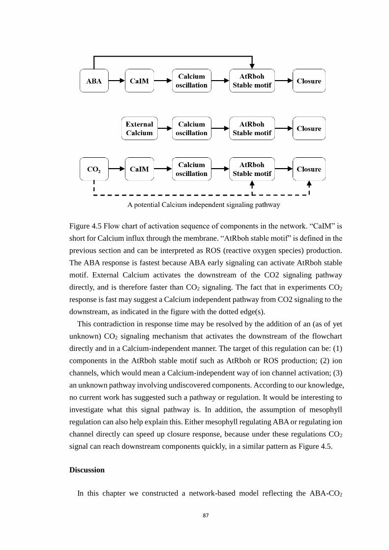
87

Figure 4.5 Flow chart of activation sequence of components in the network. “CaIM” is

short for Calcium influx through the membrane. “AtRboh stable motif” is defined in the

previous section and can be interpreted as ROS (reactive oxygen species) production.

The ABA response is fastest because ABA early signaling can activate AtRboh stable

motif. External Calcium activates the downstream of the CO2 signaling pathway

directly, and is therefore faster than CO2 signaling. The fact that in experiments CO2

response is fast may suggest a Calcium independent pathway from CO2 signaling to the

downstream, as indicated in the figure with the dotted edge(s).

This contradiction in response time may be resolved by the addition of an (as of yet

unknown) CO2 signaling mechanism that activates the downstream of the flowchart

directly and in a Calcium-independent manner. The target of this regulation can be: (1)

components in the AtRboh stable motif such as AtRboh or ROS production; (2) ion

channels, which would mean a Calcium-independent way of ion channel activation; (3)

an unknown pathway involving undiscovered components. According to our knowledge,

no current work has suggested such a pathway or regulation. It would be interesting to

investigate what this signal pathway is. In addition, the assumption of mesophyll

regulation can also help explain this. Either mesophyll regulating ABA or regulating ion

channel directly can speed up closure response, because under these regulations CO2

signal can reach downstream components quickly, in a similar pattern as Figure 4.5.

Discussion

In this chapter we constructed a network-based model reflecting the ABA-CO2

88

crosstalk in inducing stomatal closure, based on previous ABA signaling network and

knowledge of CO2 signaling in the literature. The model offers explanation to how ABA

and high CO2 induce stomatal closure, respectively. It also predicts the role of non-

canonical G-protein alpha subunits and their regulatory relationship with the canonical

G-protein alpha subunit. The crosstalk of ABA and CO2 are interpreted as combinatorial

effects in the single large SCC of the network. The SCC serves as the dynamic core and

determines the system’s long term behavior, i.e. the stomatal closure movement. The

up-stream early signaling components serve as input chains, and the down-stream ion

channels serve as chains of results. The combination of a hierarchical network backbone

structure plus a large core SCC is typical in signal transduction network.

The CO2 signaling pathway is currently under study, and there is debate on the

regulatory role of certain signaling components. For example, RHC1 is reported as a

necessary component for CO2 signaling by Tian et al.[116], in both epidermal peels and

live leaves; but a recent paper present contradicting evidence in live leaves [146]. It is

also worth pointing out that introducing mesophyll regulation (as we did) may be able

to explain different responses between epidermal peels and live leaves of rhc1 mutants.

In another paper, the authors found that unlike ABA, elevated CO2 does not activate

OST1/SnRK2 kinases in guard cells [118], while it is known that ost1 mutant is

insensitive to both ABA and CO2 [147]. The mechanism behind this remains unclear.

Further experimental evidence will reveal more information, allowing a more accurate

version of the model.

G-protein’s regulatory role in plant signal transduction is another mystery. Despite

the predictions made in the model, there are many more potential effectors of the G-

protein. Our collaborator team is performing a comprehensive test of protein-protein

interaction between G-protein alpha subunits (GPA1 and XLGs) and known signaling

components of stomatal closure, with yeast 2/3 hybrid assays, BiFC assays, and Co-IP

assays. These interaction data can help identify more potential regulators and effectors

of the G-protein alpha subunits.

Our discrete network-based modeling framework offers a promising way to uncover,

understand and predict system-level biological behavior by integration of lower-level

knowledge. It offers novel, alternative approaches to explore and predict about signal

transduction in biological systems. As the interaction data between signaling

components grow bigger and bigger, computational methods like ours will become

necessary to complement traditional methods.

89

Chapter 5 Conclusions and outlook

In this dissertation I presented my contributions in both theoretical and computational

aspects of modeling and understanding biological systems. I analyzed a multi-level

model to show its dynamic properties; I developed a general method to analyze the

attractor landscape of any finite discrete model; and I constructed a network-based

dynamic model on the crosstalk of plant responses to different environmental stress. My

work further reinforces the conclusion that of network-based modeling is a promising

pathway to understanding system-level biology.

In the first chapter of this dissertation I reviewed how network analysis and network-

based dynamic modeling can be used to determine the repertoire of cellular behaviors

associated to a within-cell network, and to identify the sub-networks that play a key role

in the cell adopting a certain behavior. Overall, the expanded network representation,

an integration of the network topology with regulatory functions, reveals the indirect

and self-sustaining influences in the system, which ultimately determine the system’s

repertoire of behaviors. The emerging answers indicate that stable motifs are a key

information processing, decision-making connectivity pattern. Stable motifs receive

information from external signals and internal perturbations, and their stabilization

serves as a point of no return in the system’s dynamics. One can characterize attractors

by the stable motifs they are determined by, and one can control the system’s outcome

by controlling stable motifs.

In the second chapter I performed analysis on the attractors of the Sun et al. stomatal

opening model, and found a very strong conclusion: under any combination of sustained

signals, all nodes in the model converge into steady states, with the potential exception

of the cytosolic Ca2+ ([Ca2+]c) and Ca2+ ATPase. Variations in the initial condition of

non-source nodes or in process timing (node update sequence) can drive at most two

nodes, PMV and Kout, into a different attractor. This high degree of attractor similarity

is somewhat unexpected, as the network has a large strongly connected component and

several feedback loops. Thus, despite the decidedly non-linear structure of the network,

most parts of the system behave in the consistent manner of a linear pathway. This is a

distinct feature of the stomatal opening model: many dynamic models of biological

systems have multiple, diverse attractors [24, 148]. The models of these systems will

evolve into drastically different attractors when starting from different initial conditions,

90

sometimes even when starting from the same initial condition, demonstrating different

biological trajectories. In the stomatal opening model, however, the uniqueness of the

steady state stomatal opening level suggests that the final extent of the stomatal opening

response is robust and resilient against changes in initial conditions or in timing. Note

that although a change in the initial condition will not change the steady-state opening

level, it may change the steady state of PMV and Kout, and may change how fast the

system converges to an attractor.

I also showed that the reduced stomatal opening model does not admit additional,

emergent oscillations or multi-stability under any biologically relevant node

perturbation (knockout or constitutive expression). I further demonstrate the robustness

of the system by examining the stomatal opening level under single node knockouts: in

most cases the signals are still likely to propagate and lead to a similar degree of stomatal

opening as in the absence of perturbation. This robustness is unlike a single linear

pathway, which would be very sensitive to node disruption. This suggests that the role

of the strongly connected components in the network could be to provide multiple paths

for the signal to propagate, but at the same time not allowing extensive multistability or

oscillations. The innovative combination of existing methods used in this work offers a

promising way to analyze multi-level models.

Following up the problem of finding attractors, I proposed and developed a general

motif-based reduction method to find both fixed points and complex attractors of any

finite discrete dynamic model, by extending an existing method from Boolean to any

discrete level. As described in Chapter 3, I established a multi-level formalism that can

identify motifs from an expanded representation of the multi-level network. Iteratively

reduction of the network according to the motifs can identify the attractors. I

demonstrated the method’s correctness and effectiveness by implementing an algorithm,

then benchmarking it on synthetic networks, and applying it to biological networks in

the literature.

The integration of the network structure and regulatory logic in the expanded network

can reveal the connectivity patterns that underlie the system’s functional repertoire.

There can be multiple extensions to this work. For example, in the Boolean case,

elementary signaling mode (ESM) has been defined from the expanded network as the

minimal set of nodes that can perform signal transduction independently [29, 32]. It can

be extended to the multi-level as well to help understand signal transduction a multi-

level expanded network. Another direction is to extend the concepts of expanded

network and stable motifs to a continuous framework. If one can distill the causal

relationships wherein a certain value of a continuous variable is sufficient to maintain a

91

certain value of another continuous variable, one can construct an expanded network

from these relationships, and obtain insight into the system’s dynamic repertoire [140].

Furthermore, one can develop the control capability of multi-level motifs. Network

controllability has multiple definitions and frameworks to address it [58, 60, 149, 150].

Motifs can be used to control the system by driving it into one of its natural attractors.

Zañudo et al. proved that in the Boolean case a sequence of stable motifs uniquely

determines an attractor, which means that driving certain nodes into their states in a

stable motif can drive the network into the corresponding attractor; they also

implemented an algorithm to identify driver nodes from Boolean stable motifs [31]. The

same principle applies to multi-level stable motifs as well, and the algorithm to find the

driver nodes to be controlled can be adapted as well. This is particularly valuable in

biological networks, as the control of stable motifs can suggest possible practical

interventions to switch the system from an undesired attractor to a desired one [25].

Another possible aspect of control is target control, i.e., driving a single node or small

set of nodes into a desired state. This can be done by exploiting more of the sufficiency

conditions revealed in an expanded network [151].

As described in Chapter 4, I constructed a network-based model reflecting the ABA-

CO2 crosstalk in inducing stomatal closure, based on previous ABA signaling network

and knowledge of CO2 signaling in the literature. We validate the model by showing

consistency between the model simulations and experimental observations. This

consistency shows the correctness of our assumed regulations, making them valid

predictions, and we propose several ways to further validate these hypotheses with

experiments. We identified the core components that causes closure by applying our

novel attractor analysis method, and thus elucidated the closure mechanism for different

signals and their crosstalk. We also perform systematic single node interventions, and a

selection of double/triple node interventions, which predict the closure responses of

mutants under a list of treatments. These intervention simulations help explain the

regulation roles of each signaling component, and predict the combinatorial effects of

interventions. In addition, we propose that introducing mesophyll regulation into the

network model can resolve the different high CO2 induced closure responses observed

between peeled epidermis and live leaves/plants. Our network-based modeling

framework offers a promising way to uncover, understand and predict system-level

biological behavior by integration of lower-level knowledge.

There have been many updates in knowledge on CO2 induced closure, and more are

expected in the near future. One of the obvious future direction is to keep updating the

model, like the Albert group did with the ABA model, according to new discoveries in

92

the signaling pathways. As the model becomes more comprehensive, the predictions,

e.g. simulations of intervention results, will further improve in accuracy. Moreover,

multi-level behavior of signaling components has been observed [118], suggesting the

potential value of developing a multi-level model, where my generalized multi-level

formalism and motifs method can apply.

This work is also a good demonstration of how to predict important regulations and

guide experiments from an in silico approach. There are too many potential regulators

and effectors for XLGs to be experimentally explored. However with the network-based

analysis, we are able to quickly identify several neccesary conditions for CO2 induced

closure, for example XLGs -| PP2Cs inhibition, and XLG → RbohD/F activation. This

points out a method how to utilize known knowledge in order to make new predictions

on less-understood regualtions. Simulations from a model can also help making

hypotheses of introducing new regulations, e.g. effect of introduction of mesophyll

regulation. Combining expertimental approaches with theoretical/computational

approaches is a promising way to understand system-level biology.

To summarize, my dissertation focuses on how to understand system-level biological

signaling with theoretical and computational approaches. Network-based discrete

modeling of biological systems, plus analyses of such models, is a promising method

toward this goal. My analysis on a complex multi-level model shows how combination

of theoretical and computational tools can reveal dynamic functions of a biological

system. To further extend the capability of theoretical and computational tools, I

developed a general modeling framework with any finite discrete levels that allows a

novel method to find attractors and control of a model. I also constructed the ABA-CO2

crosstalk model, which integrated knowledge in the literature to explain how the two

environmental signals induces closure, to predict new regulations and results of

intervention, and to generate new hypotheses. In short, my dissertation work has offered

a new and general way to analyze complex discrete models, and expanded the

understanding of the mechanism how plants respond to different environmental stress.

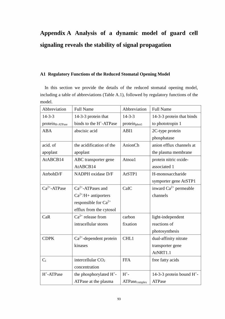
93

Appendix A Analysis of a dynamic model of guard cell

signaling reveals the stability of signal propagation

A1 Regulatory Functions of the Reduced Stomatal Opening Model

In this section we provide the details of the reduced stomatal opening model,

including a table of abbreviations (Table A.1), followed by regulatory functions of the

model.

Abbreviation Full Name Abbreviation Full Name

14-3-3

proteinH-ATPase

14-3-3 protein that

binds to the H+-ATPase

14-3-3

proteinphot1

14-3-3 protein that binds

to phototropin 1

ABA abscisic acid ABI1 2C-type protein

phosphatase

acid. of

apoplast

the acidification of the

apoplast

AnionCh anion efflux channels at

the plasma membrane

AtABCB14 ABC transporter gene

AtABCB14

Atnoa1 protein nitric oxide-

associated 1

AtrbohD/F NADPH oxidase D/F AtSTP1 H-monosaccharide

symporter gene AtSTP1

Ca2+-ATPase Ca2+-ATPases and

Ca2+/H+ antiporters

responsible for Ca2+

efflux from the cytosol

CaIC inward Ca2+ permeable

channels

CaR Ca2+ release from

intracellular stores

carbon

fixation

light-independent

reactions of

photosynthesis

CDPK Ca2+-dependent protein

kinases

CHL1 dual-affinity nitrate

transporter gene

AtNRT1.1

Ci intercellular CO2

concentration

FFA free fatty acids

H+-ATPase the phosphorylated H+-

ATPase at the plasma

H+-

ATPasecomplex

14-3-3 protein bound H+-

ATPase

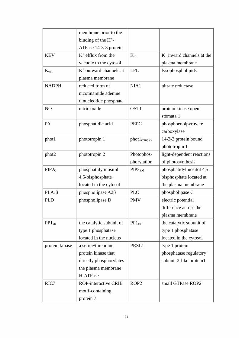
94

membrane prior to the

binding of the H+-

ATPase 14-3-3 protein

KEV K+ efflux from the

vacuole to the cytosol

Kin K+ inward channels at the

plasma membrane

Kout K+ outward channels at

plasma membrane

LPL lysophospholipids

NADPH reduced form of

nicotinamide adenine

dinucleotide phosphate

NIA1 nitrate reductase

NO nitric oxide OST1 protein kinase open

stomata 1

PA phosphatidic acid PEPC phosphoenolpyruvate

carboxylase

phot1 phototropin 1 phot1complex 14-3-3 protein bound

phototropin 1

phot2 phototropin 2 Photophos-

phorylation

light-dependent reactions

of photosynthesis

PIP2C phosphatidylinositol

4,5-bisphosphate

located in the cytosol

PIP2PM phosphatidylinositol 4,5-

bisphosphate located at

the plasma membrane

PLA2β phospholipase A2β PLC phospholipase C

PLD phospholipase D PMV electric potential

difference across the

plasma membrane

PP1cn the catalytic subunit of

type 1 phosphatase

located in the nucleus

PP1cc the catalytic subunit of

type 1 phosphatase

located in the cytosol

protein kinase a serine/threonine

protein kinase that

directly phosphorylates

the plasma membrane

H-ATPase

PRSL1 type 1 protein

phosphatase regulatory

subunit 2-like protein1

RIC7 ROP-interactive CRIB

motif-containing

protein 7

ROP2 small GTPase ROP2

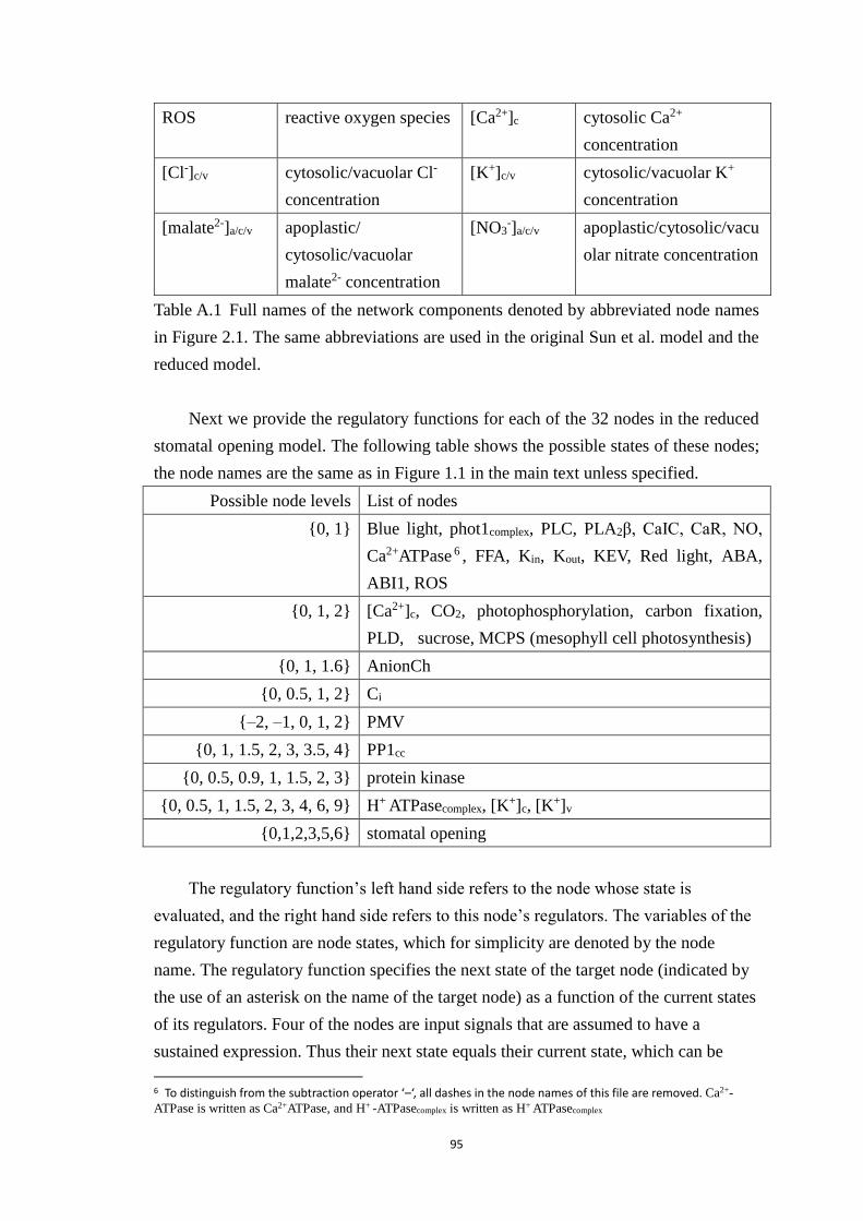
95

ROS reactive oxygen species [Ca2+]c cytosolic Ca2+

concentration

[Cl-]c/v cytosolic/vacuolar Cl-

concentration

[K+]c/v cytosolic/vacuolar K+

concentration

[malate2-]a/c/v apoplastic/

cytosolic/vacuolar

malate2- concentration

[NO3-]a/c/v apoplastic/cytosolic/vacu

olar nitrate concentration

Table A.1 Full names of the network components denoted by abbreviated node names

in Figure 2.1. The same abbreviations are used in the original Sun et al. model and the

reduced model.

Next we provide the regulatory functions for each of the 32 nodes in the reduced

stomatal opening model. The following table shows the possible states of these nodes;

the node names are the same as in Figure 1.1 in the main text unless specified.

Possible node levels List of nodes

{0, 1} Blue light, phot1complex, PLC, PLA2β, CaIC, CaR, NO,

Ca2+ATPase 6 , FFA, Kin, Kout, KEV, Red light, ABA,

ABI1, ROS

{0, 1, 2} [Ca2+]c, CO2, photophosphorylation, carbon fixation,

PLD, sucrose, MCPS (mesophyll cell photosynthesis)

{0, 1, 1.6} AnionCh

{0, 0.5, 1, 2} Ci

{–2, –1, 0, 1, 2} PMV

{0, 1, 1.5, 2, 3, 3.5, 4} PP1cc

{0, 0.5, 0.9, 1, 1.5, 2, 3} protein kinase

{0, 0.5, 1, 1.5, 2, 3, 4, 6, 9} H+ ATPasecomplex, [K+]c, [K

+]v

{0,1,2,3,5,6} stomatal opening

The regulatory function’s left hand side refers to the node whose state is

evaluated, and the right hand side refers to this node’s regulators. The variables of the

regulatory function are node states, which for simplicity are denoted by the node

name. The regulatory function specifies the next state of the target node (indicated by

the use of an asterisk on the name of the target node) as a function of the current states

of its regulators. Four of the nodes are input signals that are assumed to have a

sustained expression. Thus their next state equals their current state, which can be

6 To distinguish from the subtraction operator ‘–‘, all dashes in the node names of this file are removed. Ca2+-

ATPase is written as Ca2+ATPase, and H+ -ATPasecomplex is written as H+ ATPasecomplex

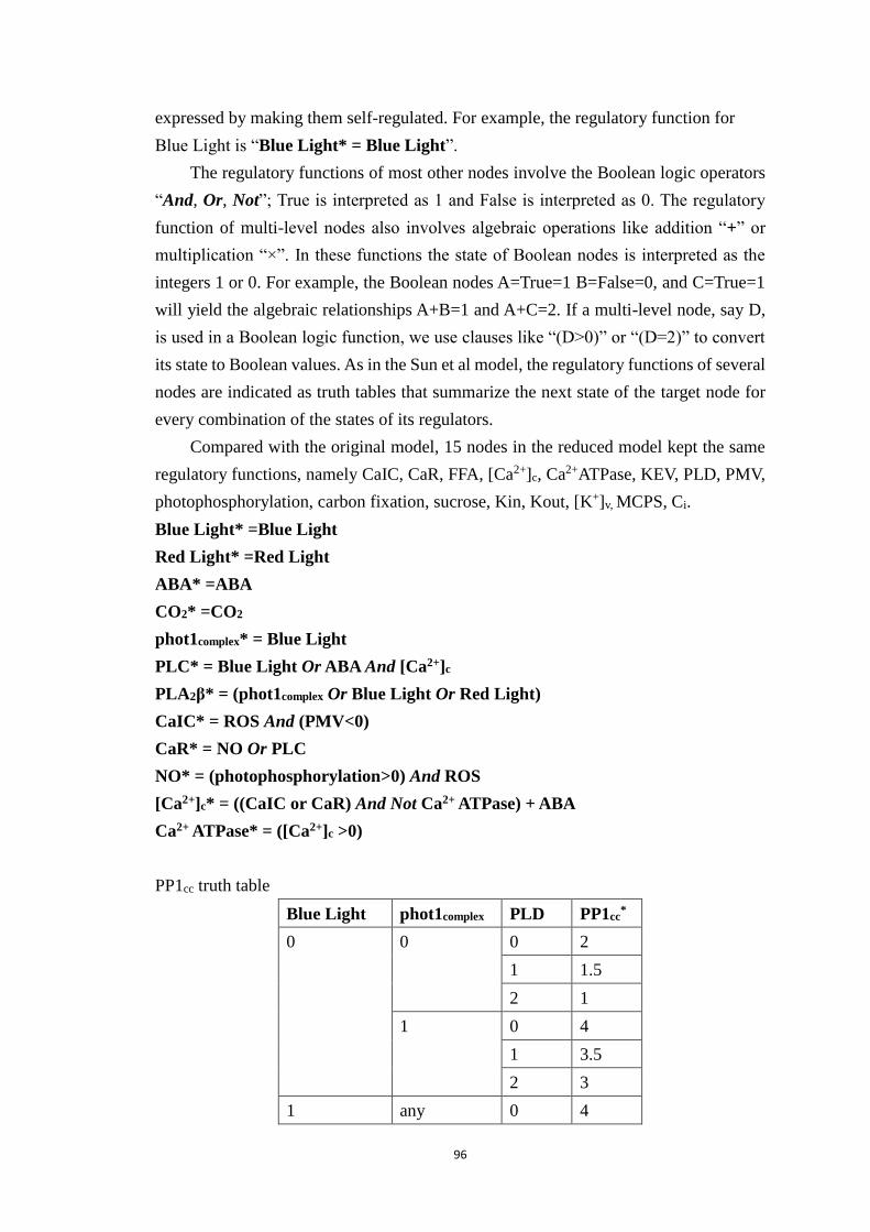
96

expressed by making them self-regulated. For example, the regulatory function for

Blue Light is “Blue Light* = Blue Light”.

The regulatory functions of most other nodes involve the Boolean logic operators

“And, Or, Not”; True is interpreted as 1 and False is interpreted as 0. The regulatory

function of multi-level nodes also involves algebraic operations like addition “+” or

multiplication “×”. In these functions the state of Boolean nodes is interpreted as the

integers 1 or 0. For example, the Boolean nodes A=True=1 B=False=0, and C=True=1

will yield the algebraic relationships A+B=1 and A+C=2. If a multi-level node, say D,

is used in a Boolean logic function, we use clauses like “(D>0)” or “(D=2)” to convert

its state to Boolean values. As in the Sun et al model, the regulatory functions of several

nodes are indicated as truth tables that summarize the next state of the target node for

every combination of the states of its regulators.

Compared with the original model, 15 nodes in the reduced model kept the same

regulatory functions, namely CaIC, CaR, FFA, [Ca2+]c, Ca2+ATPase, KEV, PLD, PMV,

photophosphorylation, carbon fixation, sucrose, Kin, Kout, [K+]v, MCPS, Ci.

Blue Light* =Blue Light

Red Light* =Red Light

ABA* =ABA

CO2* =CO2

phot1complex* = Blue Light

PLC* = Blue Light Or ABA And [Ca2+]c

PLA2β* = (phot1complex Or Blue Light Or Red Light)

CaIC* = ROS And (PMV<0)

CaR* = NO Or PLC

NO* = (photophosphorylation>0) And ROS

[Ca2+]c* = ((CaIC or CaR) And Not Ca2+ ATPase) + ABA

Ca2+ ATPase* = ([Ca2+]c >0)

PP1cc truth table

Blue Light phot1complex PLD PP1cc*

0 0 0 2

1 1.5

2 1

1 0 4

1 3.5

2 3

1 any 0 4

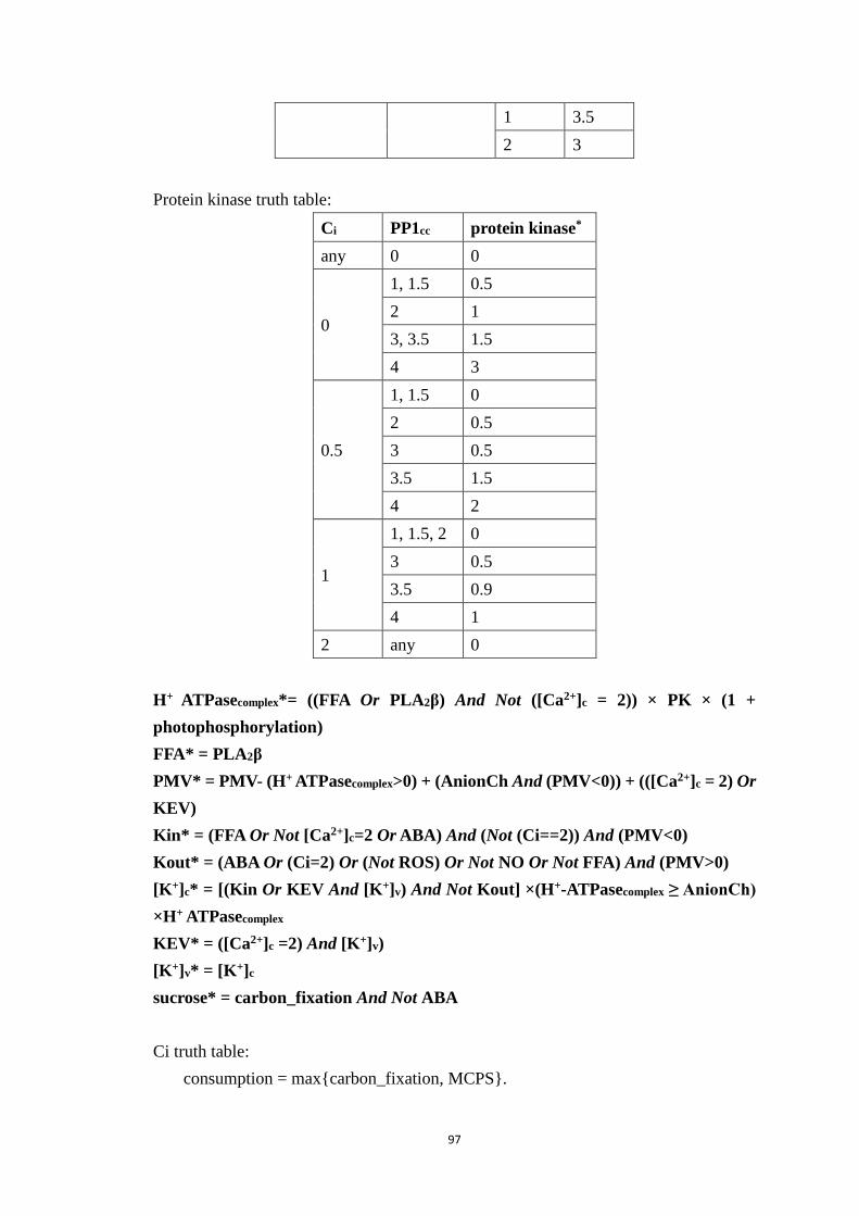
97

1 3.5

2 3

Protein kinase truth table:

Ci PP1cc protein kinase*

any 0 0

0

1, 1.5 0.5

2 1

3, 3.5 1.5

4 3

0.5

1, 1.5 0

2 0.5

3 0.5

3.5 1.5

4 2

1

1, 1.5, 2 0

3 0.5

3.5 0.9

4 1

2 any 0

H+ ATPasecomplex*= ((FFA Or PLA2β) And Not ([Ca2+]c = 2)) × PK × (1 +

photophosphorylation)

FFA* = PLA2β

PMV* = PMV- (H+ ATPasecomplex>0) + (AnionCh And (PMV<0)) + (([Ca2+]c = 2) Or

KEV)

Kin* = (FFA Or Not [Ca2+]c=2 Or ABA) And (Not (Ci==2)) And (PMV<0)

Kout* = (ABA Or (Ci=2) Or (Not ROS) Or Not NO Or Not FFA) And (PMV>0)

[K+]c* = [(Kin Or KEV And [K+]v) And Not Kout] ×(H+-ATPasecomplex ≥ AnionCh)

×H+ ATPasecomplex

KEV* = ([Ca2+]c =2) And [K+]v)

[K+]v* = [K+]c

sucrose* = carbon_fixation And Not ABA

Ci truth table:

consumption = max{carbon_fixation, MCPS}.

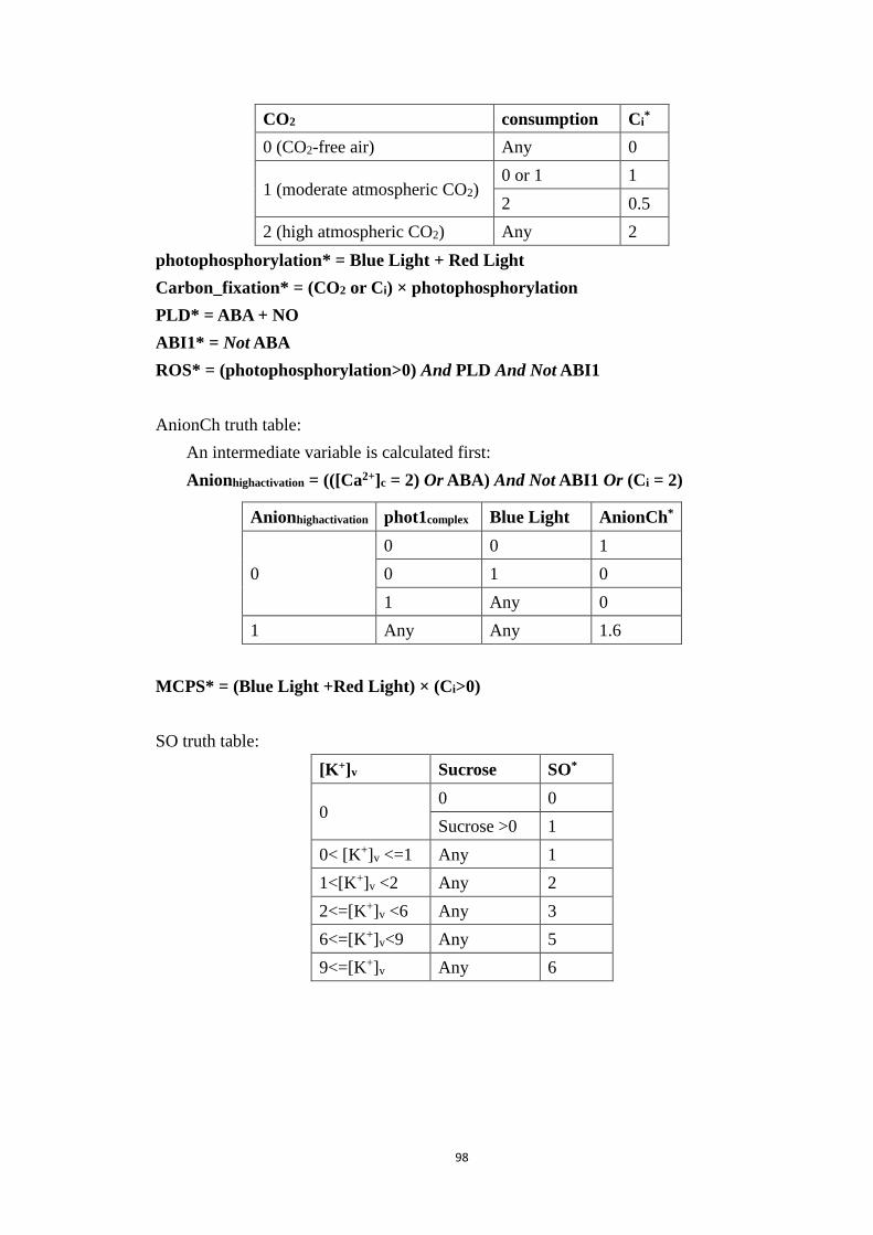
98

CO2 consumption Ci*

0 (CO2-free air) Any 0

1 (moderate atmospheric CO2) 0 or 1 1

2 0.5

2 (high atmospheric CO2) Any 2

photophosphorylation* = Blue Light + Red Light

Carbon_fixation* = (CO2 or Ci) × photophosphorylation

PLD* = ABA + NO

ABI1* = Not ABA

ROS* = (photophosphorylation>0) And PLD And Not ABI1

AnionCh truth table:

An intermediate variable is calculated first:

Anionhighactivation = (([Ca2+]c = 2) Or ABA) And Not ABI1 Or (Ci = 2)

Anionhighactivation phot1complex Blue Light AnionCh*

0

0 0 1

0 1 0

1 Any 0

1 Any Any 1.6

MCPS* = (Blue Light +Red Light) × (Ci>0)

SO truth table:

[K+]v Sucrose SO*

0 0 0

Sucrose >0 1

0< [K+]v <=1 Any 1

1<[K+]v <2 Any 2

2<=[K+]v <6 Any 3

6<=[K+]v<9 Any 5

9<=[K+]v Any 6

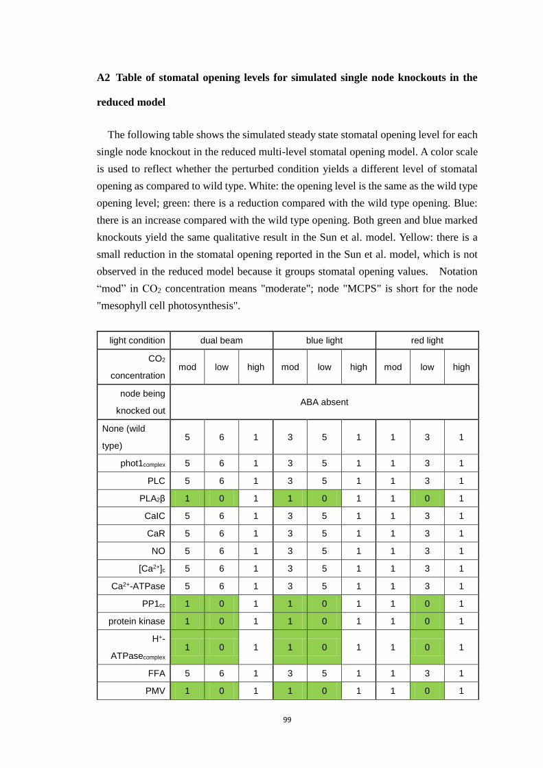
99

A2 Table of stomatal opening levels for simulated single node knockouts in the

reduced model

The following table shows the simulated steady state stomatal opening level for each

single node knockout in the reduced multi-level stomatal opening model. A color scale

is used to reflect whether the perturbed condition yields a different level of stomatal

opening as compared to wild type. White: the opening level is the same as the wild type

opening level; green: there is a reduction compared with the wild type opening. Blue:

there is an increase compared with the wild type opening. Both green and blue marked

knockouts yield the same qualitative result in the Sun et al. model. Yellow: there is a

small reduction in the stomatal opening reported in the Sun et al. model, which is not

observed in the reduced model because it groups stomatal opening values. Notation

“mod” in CO2 concentration means "moderate"; node "MCPS" is short for the node

"mesophyll cell photosynthesis".

light condition dual beam blue light red light

CO2

concentration mod low high mod low high mod low high

node being

knocked out ABA absent

None (wild

type) 5 6 1 3 5 1 1 3 1

phot1complex 5 6 1 3 5 1 1 3 1

PLC 5 6 1 3 5 1 1 3 1

PLA2β 1 0 1 1 0 1 1 0 1

CaIC 5 6 1 3 5 1 1 3 1

CaR 5 6 1 3 5 1 1 3 1

NO 5 6 1 3 5 1 1 3 1

[Ca2+]c 5 6 1 3 5 1 1 3 1

Ca2+-ATPase 5 6 1 3 5 1 1 3 1

PP1cc 1 0 1 1 0 1 1 0 1

protein kinase 1 0 1 1 0 1 1 0 1

H+-

ATPasecomplex 1 0 1 1 0 1 1 0 1

FFA 5 6 1 3 5 1 1 3 1

PMV 1 0 1 1 0 1 1 0 1

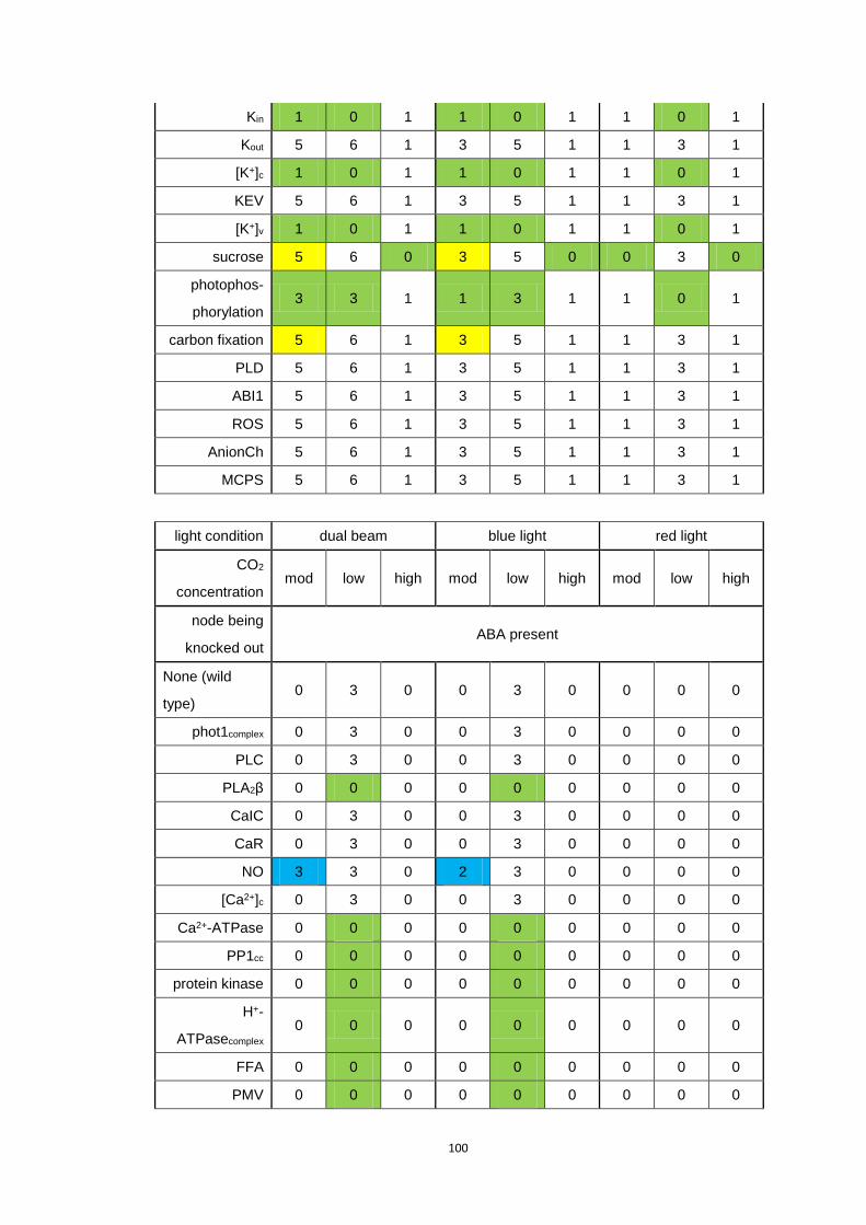
100

Kin 1 0 1 1 0 1 1 0 1

Kout 5 6 1 3 5 1 1 3 1

[K+]c 1 0 1 1 0 1 1 0 1

KEV 5 6 1 3 5 1 1 3 1

[K+]v 1 0 1 1 0 1 1 0 1

sucrose 5 6 0 3 5 0 0 3 0

photophos-

phorylation 3 3 1 1 3 1 1 0 1

carbon fixation 5 6 1 3 5 1 1 3 1

PLD 5 6 1 3 5 1 1 3 1

ABI1 5 6 1 3 5 1 1 3 1

ROS 5 6 1 3 5 1 1 3 1

AnionCh 5 6 1 3 5 1 1 3 1

MCPS 5 6 1 3 5 1 1 3 1

light condition dual beam blue light red light

CO2

concentration mod low high mod low high mod low high

node being

knocked out ABA present

None (wild

type) 0 3 0 0 3 0 0 0 0

phot1complex 0 3 0 0 3 0 0 0 0

PLC 0 3 0 0 3 0 0 0 0

PLA2β 0 0 0 0 0 0 0 0 0

CaIC 0 3 0 0 3 0 0 0 0

CaR 0 3 0 0 3 0 0 0 0

NO 3 3 0 2 3 0 0 0 0

[Ca2+]c 0 3 0 0 3 0 0 0 0

Ca2+-ATPase 0 0 0 0 0 0 0 0 0

PP1cc 0 0 0 0 0 0 0 0 0

protein kinase 0 0 0 0 0 0 0 0 0

H+-

ATPasecomplex 0 0 0 0 0 0 0 0 0

FFA 0 0 0 0 0 0 0 0 0

PMV 0 0 0 0 0 0 0 0 0

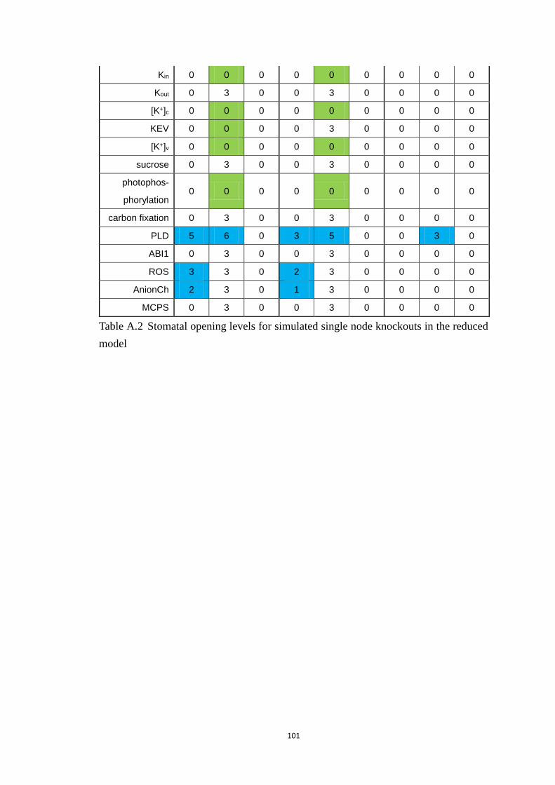
101

Kin 0 0 0 0 0 0 0 0 0

Kout 0 3 0 0 3 0 0 0 0

[K+]c 0 0 0 0 0 0 0 0 0

KEV 0 0 0 0 3 0 0 0 0

[K+]v 0 0 0 0 0 0 0 0 0

sucrose 0 3 0 0 3 0 0 0 0

photophos-

phorylation 0 0 0 0 0 0 0 0 0

carbon fixation 0 3 0 0 3 0 0 0 0

PLD 5 6 0 3 5 0 0 3 0

ABI1 0 3 0 0 3 0 0 0 0

ROS 3 3 0 2 3 0 0 0 0

AnionCh 2 3 0 1 3 0 0 0 0

MCPS 0 3 0 0 3 0 0 0 0

Table A.2 Stomatal opening levels for simulated single node knockouts in the reduced

model

102

Appendix B A general method to find the

attractors of discrete dynamic models of

biological systems

B1 Runtime performance of the multi-level Quine-McCluskey algorithm

The computational complexity of the Boolean Quine–McCluskey algorithm grows

exponentially with the number of variables, because the problem it solves is NP-hard,

and it is shown that the upper bound on the number of prime implicants of a Boolean

function with n variables is 3n ln(𝑛) [152]. Since a Boolean function is a special case

of a discrete function , it is straightforward that finding all prime implicants of a multi-

level function is at least as complex as finding all prime implicants of a Boolean function.

To test whether the multi-level QM algorithm is capable of analyzing biological network

models, we benchmark how long it takes for the algorithm to transform all node

functions on 100 randomly generated heterogeneous networks. The networks have 50

nodes and have a power law in-degree distribution with exponent -3 and maximum

degree 8. Each node has 60% chance of having 2 states, 25% chance of having 3 states,

10% chance of having 4 states, and 5% chance of having 5 states. These parameters

exceed the complexity of current multi-level biological models. The result is shown in

Figure B.1: the multi-level QM algorithm can effectively transform the functions. In

addition, we found that within the algorithm, the complexity of identifying stable or

oscillating motifs is much more than that of the QM transformation. So we conclude

that the complexity of the QM algorithm is acceptable for practical problems.

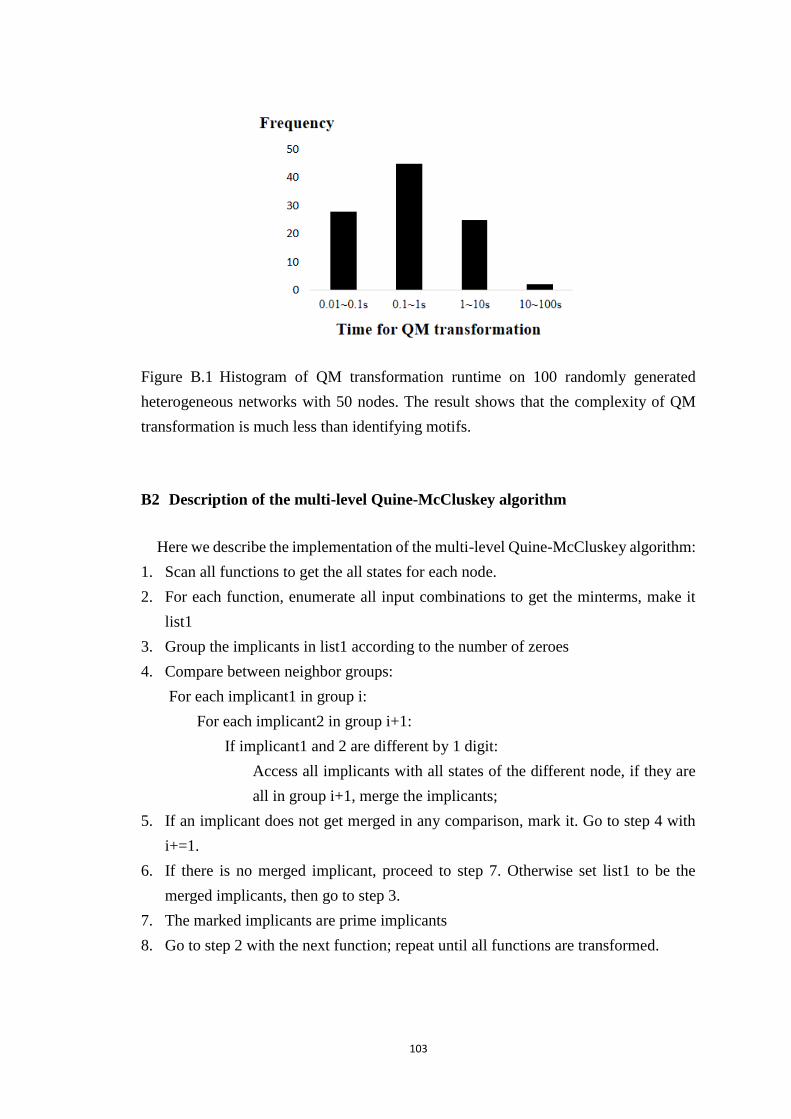
103

Figure B.1 Histogram of QM transformation runtime on 100 randomly generated

heterogeneous networks with 50 nodes. The result shows that the complexity of QM

transformation is much less than identifying motifs.

B2 Description of the multi-level Quine-McCluskey algorithm

Here we describe the implementation of the multi-level Quine-McCluskey algorithm:

1. Scan all functions to get the all states for each node.

2. For each function, enumerate all input combinations to get the minterms, make it

list1

3. Group the implicants in list1 according to the number of zeroes

4. Compare between neighbor groups:

For each implicant1 in group i:

For each implicant2 in group i+1:

If implicant1 and 2 are different by 1 digit:

Access all implicants with all states of the different node, if they are

all in group i+1, merge the implicants;

5. If an implicant does not get merged in any comparison, mark it. Go to step 4 with

i+=1.

6. If there is no merged implicant, proceed to step 7. Otherwise set list1 to be the

merged implicants, then go to step 3.

7. The marked implicants are prime implicants

8. Go to step 2 with the next function; repeat until all functions are transformed.

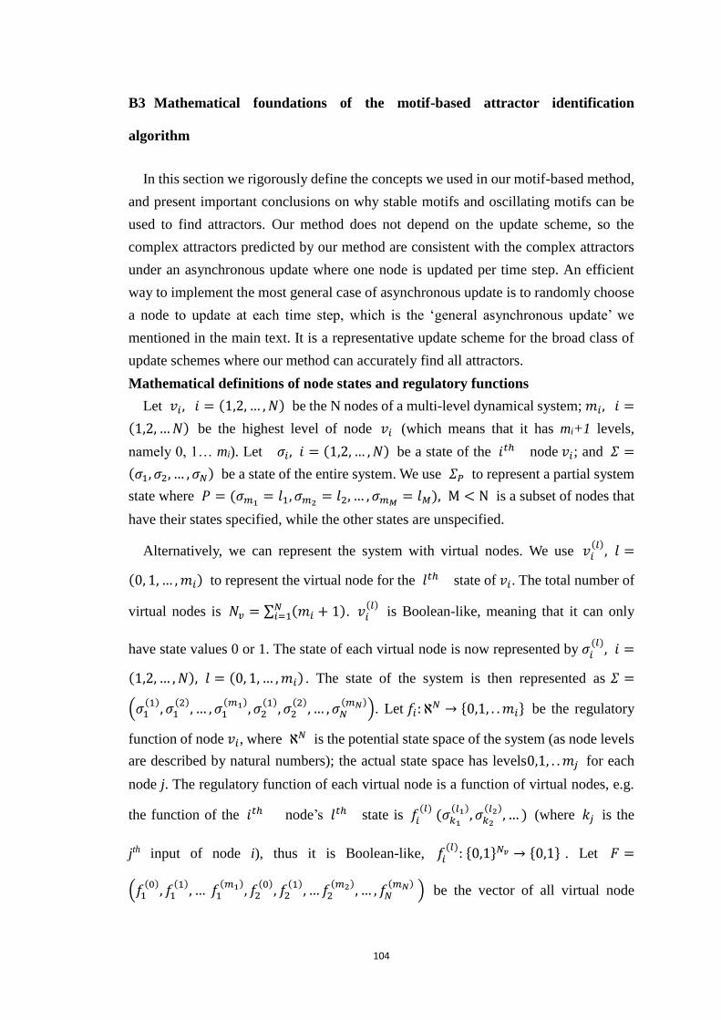
104

B3 Mathematical foundations of the motif-based attractor identification

algorithm

In this section we rigorously define the concepts we used in our motif-based method,

and present important conclusions on why stable motifs and oscillating motifs can be

used to find attractors. Our method does not depend on the update scheme, so the

complex attractors predicted by our method are consistent with the complex attractors

under an asynchronous update where one node is updated per time step. An efficient

way to implement the most general case of asynchronous update is to randomly choose

a node to update at each time step, which is the ‘general asynchronous update’ we

mentioned in the main text. It is a representative update scheme for the broad class of

update schemes where our method can accurately find all attractors.

Mathematical definitions of node states and regulatory functions

Let 𝑣𝑖 , 𝑖 = (1,2, … , 𝑁) be the N nodes of a multi-level dynamical system; 𝑚𝑖, 𝑖 =

(1,2, … 𝑁) be the highest level of node 𝑣𝑖 (which means that it has mi+1 levels,

namely 0, 1… mi). Let 𝜎𝑖, 𝑖 = (1,2, … , 𝑁) be a state of the 𝑖𝑡ℎ node 𝑣𝑖; and 𝛴 =

(𝜎1, 𝜎2, … , 𝜎𝑁) be a state of the entire system. We use 𝛴𝑃 to represent a partial system

state where 𝑃 = (𝜎𝑚1= 𝑙1, 𝜎𝑚2

= 𝑙2, … , 𝜎𝑚𝑀= 𝑙𝑀), M < N is a subset of nodes that

have their states specified, while the other states are unspecified.

Alternatively, we can represent the system with virtual nodes. We use 𝑣𝑖(𝑙)

, 𝑙 =

(0, 1, … , 𝑚𝑖) to represent the virtual node for the 𝑙𝑡ℎ state of 𝑣𝑖. The total number of

virtual nodes is 𝑁𝑣 = ∑ (𝑚𝑖 + 1)𝑁𝑖=1 . 𝑣𝑖

(𝑙) is Boolean-like, meaning that it can only

have state values 0 or 1. The state of each virtual node is now represented by 𝜎𝑖(𝑙)

, 𝑖 =

(1,2, … , 𝑁), 𝑙 = (0, 1, … , 𝑚𝑖) . The state of the system is then represented as 𝛴 =

(𝜎1(1)

, 𝜎1(2)

, … , 𝜎1(𝑚1)

, 𝜎2(1)

, 𝜎2(2)

, … , 𝜎𝑁(𝑚𝑁)

). Let 𝑓𝑖: ℵ𝑁 → {0,1, . . 𝑚𝑖} be the regulatory

function of node 𝑣𝑖, where ℵ𝑁 is the potential state space of the system (as node levels

are described by natural numbers); the actual state space has levels0,1, . . 𝑚𝑗 for each

node j. The regulatory function of each virtual node is a function of virtual nodes, e.g.

the function of the 𝑖𝑡ℎ node’s 𝑙𝑡ℎ state is 𝑓𝑖(𝑙)

(𝜎𝑘1

(𝑙1), 𝜎𝑘2

(𝑙2), … ) (where 𝑘𝑗 is the

jth input of node i), thus it is Boolean-like, 𝑓𝑖(𝑙)

: {0,1}𝑁𝑣 → {0,1} . Let 𝐹 =

(𝑓1(0)

, 𝑓1(1)

, … 𝑓1(𝑚1)

, 𝑓2(0)

, 𝑓2(1)

, … 𝑓2(𝑚2)

, … , 𝑓𝑁(𝑚𝑁)

) be the vector of all virtual node

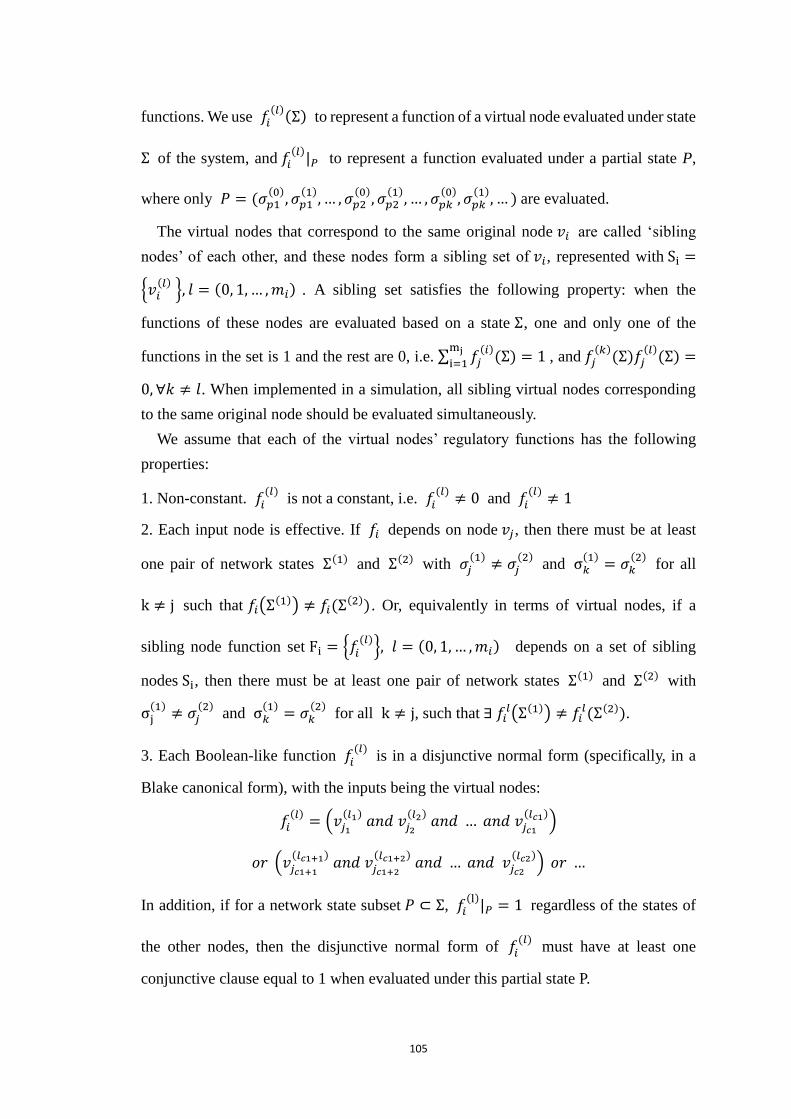
105

functions. We use 𝑓𝑖(𝑙)

(Σ) to represent a function of a virtual node evaluated under state

Σ of the system, and 𝑓𝑖(𝑙)

|𝑃 to represent a function evaluated under a partial state P,

where only 𝑃 = (𝜎𝑝1(0)

, 𝜎𝑝1(1)

, … , 𝜎𝑝2(0)

, 𝜎𝑝2(1)

, … , 𝜎𝑝𝑘(0)

, 𝜎𝑝𝑘(1)

, … ) are evaluated.

The virtual nodes that correspond to the same original node 𝑣𝑖 are called ‘sibling

nodes’ of each other, and these nodes form a sibling set of 𝑣𝑖, represented with Si =

{𝑣𝑖(𝑙)

}, 𝑙 = (0, 1, … , 𝑚𝑖) . A sibling set satisfies the following property: when the

functions of these nodes are evaluated based on a state Σ, one and only one of the

functions in the set is 1 and the rest are 0, i.e. ∑ 𝑓𝑗(𝑖)

(Σ)mj

i=1= 1 , and 𝑓𝑗

(𝑘)(Σ)𝑓𝑗

(𝑙)(Σ) =

0, ∀𝑘 ≠ 𝑙. When implemented in a simulation, all sibling virtual nodes corresponding

to the same original node should be evaluated simultaneously.

We assume that each of the virtual nodes’ regulatory functions has the following

properties:

1. Non-constant. 𝑓𝑖(𝑙)

is not a constant, i.e. 𝑓𝑖(𝑙)

≠ 0 and 𝑓𝑖(𝑙)

≠ 1

2. Each input node is effective. If 𝑓𝑖 depends on node 𝑣𝑗 , then there must be at least

one pair of network states Σ(1) and Σ(2) with 𝜎𝑗(1)

≠ 𝜎𝑗(2)

and σ𝑘(1)

= 𝜎𝑘(2)

for all

k ≠ j such that 𝑓𝑖(Σ(1)) ≠ 𝑓𝑖(Σ(2)). Or, equivalently in terms of virtual nodes, if a

sibling node function set Fi = {𝑓𝑖(𝑙)

}, 𝑙 = (0, 1, … , 𝑚𝑖) depends on a set of sibling

nodes Si, then there must be at least one pair of network states Σ(1) and Σ(2) with

σj(1)

≠ 𝜎𝑗(2)

and σ𝑘(1)

= 𝜎𝑘(2)

for all k ≠ j, such that ∃ 𝑓𝑖𝑙(Σ(1)) ≠ 𝑓𝑖

𝑙(Σ(2)).

3. Each Boolean-like function 𝑓𝑖(𝑙)

is in a disjunctive normal form (specifically, in a

Blake canonical form), with the inputs being the virtual nodes:

𝑓𝑖(𝑙)

= (𝑣𝑗1

(𝑙1) 𝑎𝑛𝑑 𝑣𝑗2

(𝑙2) 𝑎𝑛𝑑 … 𝑎𝑛𝑑 𝑣𝑗𝑐1

(𝑙𝑐1))

𝑜𝑟 (𝑣𝑗𝑐1+1

(𝑙𝑐1+1) 𝑎𝑛𝑑 𝑣𝑗𝑐1+2

(𝑙𝑐1+2) 𝑎𝑛𝑑 … 𝑎𝑛𝑑 𝑣𝑗𝑐2

(𝑙𝑐2)) 𝑜𝑟 …

In addition, if for a network state subset 𝑃 ⊂ Σ, 𝑓𝑖(l)|𝑃 = 1 regardless of the states of

the other nodes, then the disjunctive normal form of 𝑓𝑖(𝑙)

must have at least one

conjunctive clause equal to 1 when evaluated under this partial state P.

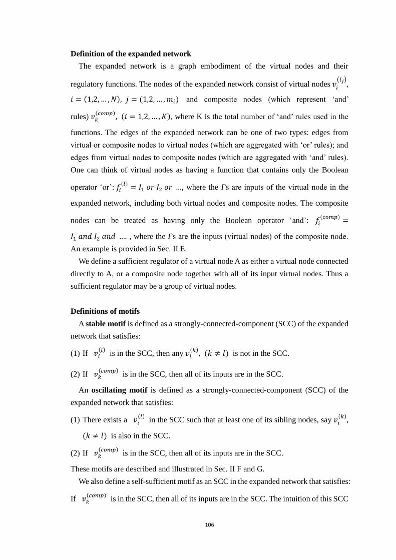
106

Definition of the expanded network

The expanded network is a graph embodiment of the virtual nodes and their

regulatory functions. The nodes of the expanded network consist of virtual nodes 𝑣𝑖

(𝑙𝑗),

𝑖 = (1,2, … , 𝑁), 𝑗 = (1,2, … , 𝑚𝑖) and composite nodes (which represent ‘and’

rules) 𝑣𝑘(𝑐𝑜𝑚𝑝)

, (𝑖 = 1,2, … , 𝐾), where K is the total number of ‘and’ rules used in the

functions. The edges of the expanded network can be one of two types: edges from

virtual or composite nodes to virtual nodes (which are aggregated with ‘or’ rules); and

edges from virtual nodes to composite nodes (which are aggregated with ‘and’ rules).

One can think of virtual nodes as having a function that contains only the Boolean

operator ‘or’: 𝑓𝑖(𝑙)

= 𝐼1 𝑜𝑟 𝐼2 𝑜𝑟 …, where the I’s are inputs of the virtual node in the

expanded network, including both virtual nodes and composite nodes. The composite

nodes can be treated as having only the Boolean operator ‘and’: 𝑓𝑖(𝑐𝑜𝑚𝑝)

=

𝐼1 𝑎𝑛𝑑 𝐼2 𝑎𝑛𝑑 …. , where the I’s are the inputs (virtual nodes) of the composite node.

An example is provided in Sec. II E.

We define a sufficient regulator of a virtual node A as either a virtual node connected

directly to A, or a composite node together with all of its input virtual nodes. Thus a

sufficient regulator may be a group of virtual nodes.

Definitions of motifs

A stable motif is defined as a strongly-connected-component (SCC) of the expanded

network that satisfies:

(1) If 𝑣𝑖(𝑙)

is in the SCC, then any 𝑣𝑖(𝑘)

, (𝑘 ≠ 𝑙) is not in the SCC.

(2) If 𝑣𝑘(𝑐𝑜𝑚𝑝)

is in the SCC, then all of its inputs are in the SCC.

An oscillating motif is defined as a strongly-connected-component (SCC) of the

expanded network that satisfies:

(1) There exists a 𝑣𝑖(𝑙)

in the SCC such that at least one of its sibling nodes, say 𝑣𝑖(𝑘)

,

(𝑘 ≠ 𝑙) is also in the SCC.

(2) If 𝑣𝑘(𝑐𝑜𝑚𝑝)

is in the SCC, then all of its inputs are in the SCC.

These motifs are described and illustrated in Sec. II F and G.

We also define a self-sufficient motif as an SCC in the expanded network that satisfies:

If 𝑣𝑘(𝑐𝑜𝑚𝑝)

is in the SCC, then all of its inputs are in the SCC. The intuition of this SCC

107

is that it is a self-sustaining feedback loop. Stable motifs and oscillating motifs are

special self-sufficient motifs, with extra requirements in the states involved in the motif.

It is important to note that both stable motifs and oscillating motifs correspond to SCCs

in the original network. Stable motifs are SCCs in which all cycles are positive.

Oscillating motifs contain negative cycles. These negative cycles may only be apparent

when considering the specific regulatory functions.

In analogy to source nodes (i.e. nodes that do not have incoming edges), we call an

SCC a source SCC if there are no nodes other than the nodes of the SCC that can reach

the source SCC through directed paths.

There is a one-to-one correspondence between stable motifs and partial fixed

points

We define a partial fixed point (or partial steady state), as a set of nodes and associated

states in which the nodes stabilize regardless of the rest of the network. Note that this

definition expresses a stricter condition than a set of nodes whose states stabilizes in a

certain context (which depends on the rest of the network).

We show that each stable motif corresponds to a partial fixed point of the system, and

that each partial fixed point corresponds to a stable motif.

Proposition 1. A stable motif corresponds to a fixed point of the nodes that participate

in the motif, i.e. the states of the nodes of the stable motif remain the same regardless

of the state of the other nodes. Formally,

Let 𝑀 = (𝑣𝑗1

(𝑙1), 𝑣𝑗2

(𝑙2), … , 𝑣𝑗𝑘

(𝑙𝑘), 𝑣𝑚1

(𝑐𝑜𝑚𝑝), 𝑣𝑚2

(𝑐𝑜𝑚𝑝), … , 𝑣𝑚𝐿

(𝑐𝑜𝑚𝑝)) be a stable motif where

𝑣𝑗1

(𝑙1), 𝑣𝑗2

(𝑙2), … , 𝑣𝑗𝑘

(𝑙𝑘) are virtual nodes and 𝑣𝑚1

(𝑐𝑜𝑚𝑝), 𝑣𝑚2

(𝑐𝑜𝑚𝑝), … , 𝑣𝑚𝐿

(𝑐𝑜𝑚𝑝) are composite

nodes. Let 𝑃 = (𝜎𝑗1= 𝑙1, 𝜎𝑗𝑘

= 𝑙𝑘, … , 𝜎𝑗𝑘= 𝑙𝑘) be a partial system state. Then for any

system state 𝛴𝑃 with 𝜎𝑗𝑖= 𝑙𝑖, we have 𝑓𝑗𝑖

(𝑙𝑘)(𝛴𝑃) = 𝛿𝑖𝑘.

Sketch of proof: We first show that 𝑓𝑗𝑖

(𝑙𝑖)(Σ𝑃) = 1. By definition of a stable motif, each

virtual node’s function must have a conjunctive clause (implicant) that consists of either

of the following: (1) a virtual node of the same stable motif; or (2) a composite node

whose inputs consists only of virtual nodes of the same stable motif. This implicant will

be 1 when 𝑓𝑗𝑖

(𝑙𝑖)(Σ𝑃) is evaluated, fixing the value 𝑓𝑗𝑖

(𝑙𝑖)(Σ𝑃) = 1. Then 𝑓𝑗𝑖

(𝑙𝑘)(Σ𝑀) =

0 ∀𝑘 ≠ 𝑖 is trivially true because the functions of sibling nodes must

108

satisfy: 𝑓𝑗(𝑘)

(Σ)𝑓𝑗(𝑙)

(Σ) = 0 ∀𝑘 ≠ 𝑙.

Proposition 2. (Reverse of proposition 1) For any partial fixed point of the system, i.e.

a set of node states where updating any involved node gives back the same state for the

node, there is a set of stable motifs that correspond to it. Formally,

Let 𝑃 = (𝜎𝑗1= 𝑙1, 𝜎𝑗𝑘

= 𝑙𝑘, … , 𝜎𝑗𝑘= 𝑙𝑘) be a partial system state such

that 𝑓𝑗𝑖

(𝑙𝑖)(𝛴𝑃) = 1, ∀𝑗𝑖. Then (1) there exists a set of stable motifs {𝑀𝑛} where each

stable motif contains only nodes from {𝑣𝑗𝑖

𝑙𝑖}, 𝑖 = 1, … , 𝑘 as virtual nodes; (2) the nodes

specified in P but not in nodes of {𝑀𝑛} are downstream of the nodes of {𝑀𝑛}.

Sketch of proof: From the disjunctive normal form of the functions, 𝑓𝑗𝑖

(𝑙𝑖)(Σ𝑃) = 1

means that at least one of the conjunctive clauses of each function is 1, and consists of

virtual nodes specified in P. Then one can create a sub-network of the expanded network,

whose nodes are these virtual nodes as well as composite nodes representing

conjunctive clauses; and edges are added if a virtual node or composite node is an input

in a virtual node’s function, or if a virtual node is an input of a composite node. Since

each virtual node in this sub-network has at least one input within the sub-network, there

exists at least one SCC. This SCC(s) is/are the stable motif(s) we are looking for.

Stable and oscillating parts of complex attractors

A complex attractor of the whole system consists of a set of states that the system

keeps revisiting. When considering the states visited by each node in a complex attractor,

there may be a subset of nodes whose state remains the same. We call these nodes

stabilized nodes. The remaining nodes (potentially, all nodes) will oscillate, meaning

that they will keep revisiting all, or possibly a subset, of their states. We will call these

nodes oscillating nodes. In the following two propositions we establish the relationships

between these nodes.

Proposition 3. Stabilized nodes in an attractor can be downstream of stabilized nodes

or downstream of oscillating nodes.

Let 𝐴 be an attractor of a multi-level dynamical system under general asynchronous

update, and let 𝑆 and 𝑂 be the stabilized and oscillating nodes, respectively. If 𝑣𝑠 ⊂

𝑆 and 𝑙𝑠 is the node’s stabilized value, then one of the following holds: (1) one of the

conjunctive clauses of 𝑓𝑠(𝑙𝑠)

depends only on nodes of 𝑆 in 𝐴; if (1) is not true, then (2)

109

𝑓𝑠(𝑙𝑠)

and the function of at least one sibling node 𝑓𝑠(𝑘𝑠)

, 𝑘𝑠 ≠ 𝑙𝑠 have at least one

conjunctive clause dependent on the nodes in O.

The first case is self-evident. An example for the second case is a network with Boolean

nodes, A, B and C:

𝑓𝐴(0)

= (𝐴1 or 𝐵1) 𝑎𝑛𝑑 𝐶0,

𝑓𝐴(1)

= 𝐴0 𝑎𝑛𝑑 𝐵0 𝑜𝑟 𝐶1,

𝑓𝐵(0)

= (𝐴1 or 𝐵1) 𝑎𝑛𝑑 𝐶0,

𝑓𝐵(1)

= 𝐴0 𝑎𝑚𝑑 𝐵0 𝑜𝑟 𝐶1,

𝑓𝐶(0)

= 𝐵0 𝑎𝑛𝑑 𝐶0 𝑜𝑟 𝐴0 𝑎𝑛𝑑 𝐶0,

𝑓𝐶(1)

= (𝐴1 𝑎𝑛𝑑 𝐵1) 𝑜𝑟 𝐶1,

where for simplicity the virtual nodes are denoted Xi, X={A,B,C} instead of Xi. This

network has an oscillating attractor with A and B oscillating and C stabilized at 0. C is

stabilized despite being regulated by nodes that oscillate. It does not satisfy (1) in the

proposition; instead, 𝑓𝐶(0)

and 𝑓𝐶(1)

satisfy (2) in the proposition.

Proposition 4. Oscillating nodes in an attractor must be downstream of oscillating

nodes.

Let 𝐴 be an attractor of a multi-level dynamical system under general asynchronous

update, and let 𝑆 and 𝑂 be the stabilized and oscillating nodes, respectively. If 𝑣𝑂 ⊂

𝑂 and 𝑙𝑂1, 𝑙𝑂2

, … , 𝑙𝑂𝑘 are the oscillating states, then the following holds: none of the

conjunctive clauses of 𝑓𝑂𝑖

(𝑙𝑂𝑖), (𝑖 = 1,2, … , 𝑘) depends only on nodes of 𝑆 in 𝐴; or

alternatively, all functions 𝑓𝑂𝑖

(𝑙𝑂𝑖), (𝑖 = 1,2, … , 𝑘) have at least one conjunctive clause

dependent on state of nodes in O.

The proof for proposition 4 is straightforward.

Iterative stable motif based network reduction conserves the attractors of the system

We proceed to the proof of conservation of attractors during iterative network reduction

by stating three lemmas.

Lemma 1. Construction of the stabilized set 𝑆𝑟𝑒𝑑 that corresponds to at least one stable

motif

110

Let 𝐴 be an attractor of a multi-level dynamical system under general asynchronous

update, and let 𝑆 and 𝑂 be the stabilized and oscillating nodes, respectively. If there

is a partial fixed point in A, then: there exists a set of nodes 𝑆𝑟𝑒𝑑 ⊂ 𝑆 such that in the

expanded network representation there will be at least one stable motif composed only

of virtual nodes of 𝑆𝑟𝑒𝑑 in A, or composite nodes composed of such nodes.

Sketch of proof: Each stabilized node in S corresponds to a function 𝑓S(ls)

. By

Proposition 3, we can divide S into nodes whose functions have a conjunctive clause

that depends only on node states (virtual nodes) specified in S, denoted 𝑆0, and nodes

that have at least one conjunctive clause in their rule dependent on the states of nodes

in O, denoted 𝑆𝑜𝑠𝑐. Let 𝑆1 ⊂ 𝑆0 be the nodes that have at least one conjunctive clause

dependent only on nodes’ states specified in 𝑆0. Let 𝑆2 ⊂ 𝑆1 be the nodes that have at

least one conjunctive clause dependent only on node states specified in 𝑆1. One can do

this iteratively until 𝑆𝑖𝑚𝑎𝑥= 𝑆𝑖𝑚𝑎𝑥+1 , and denote 𝑆𝑟𝑒𝑑 = 𝑆𝑖𝑚𝑎𝑥

. Since there exists a

partial fixed point, 𝑆𝑟𝑒𝑑 will contain nodes in the partial fixed point and will not be an

empty set. The iterative selection guarantees that 𝑆𝑟𝑒𝑑 does not depend on oscillating

nodes or nodes influenced by oscillating nodes. And since the function of each node in

𝑆𝑟𝑒𝑑 contains at least one conjunctive clause dependent only on nodes in 𝑆𝑟𝑒𝑑 itself,

there is at least one SCC in 𝑆𝑟𝑒𝑑 and this SCC satisfies the definition of a stable motif.

Lemma 2. Network reduction based on stable motifs stabilizes the nodes in 𝑆𝑟𝑒𝑑

Let 𝑆𝑟𝑒𝑑 ⊂ 𝑆 be the set of nodes constructed in Lemma 1. Then (1) Network reduction

based on stable motifs composed only of nodes from 𝑆𝑟𝑒𝑑 can only stabilize nodes

in 𝑆𝑟𝑒𝑑 . Moreover, (2) if a node i in 𝑆𝑟𝑒𝑑 stabilizes during the reduction, it has to

stabilize at its state specified in A; if a node i does not stabilize during the reduction,

then after the reduction, its function 𝑓𝑖(𝑙𝑠)

, where 𝑙𝑠 is the node’s stabilized state in A,

must have a conjunctive clause that depends only on nodes’ states specified in 𝑆𝑟𝑒𝑑 in

A that did not stabilize during reduction.

Sketch of proof: We first prove (1) by showing that the other nodes, i.e. nodes in S0 −

𝑆𝑟𝑒𝑑 and 𝑆𝑜𝑠𝑐, cannot stabilize from stable motifs composed only of nodes from 𝑆𝑟𝑒𝑑.

This statement is straightforward from the definitions of S0 − 𝑆𝑟𝑒𝑑 and 𝑆𝑜𝑠𝑐. Nodes

in S0 − 𝑆𝑟𝑒𝑑 do not have any conjunctive clauses that depend only on nodes’ states

from 𝑆𝑟𝑒𝑑, otherwise the nodes would be in 𝑆𝑟𝑒𝑑. According to Proposition 3, nodes

in 𝑆𝑜𝑠𝑐 do not have any conjunctive clauses that depend only on nodes’ states from 𝑆𝑟𝑒𝑑.

Therefore reduction based on stable motifs composed only of nodes from 𝑆𝑟𝑒𝑑 is not

sufficient to stabilize these nodes. To show (2), consider the iterative process of

111

reduction by plugging in the stabilized nodes’ states. One starts with a chosen SCC

in 𝑆𝑟𝑒𝑑, and then nodes with at least one conjunctive clause depending only on nodes

states from 𝑆𝑟𝑒𝑑 will stabilize in their value in A. When this reduction is applied

iteratively until it cannot be done anymore, the resulting 𝑆𝑟𝑒𝑑 contains only non-

stabilized nodes, whose functions do not have any dependence on the reduced nodes.

Then these functions must have a conjunctive clause that depends only on nodes’ states

specified in 𝑆𝑟𝑒𝑑 in A that did not stabilize during reduction.

Lemma 3. In a system/reduced system with no stable motifs, all nodes are influenced

by oscillating nodes.

Let 𝐴 be an attractor of a multi-level dynamical system under general asynchronous

update, and let 𝑆 and 𝑂 be the stabilized and oscillating nodes, respectively.

Let 𝑆𝑟𝑒𝑑 ⊂ 𝑆 be the set of nodes constructed in Lemma 1. Assume 𝑆𝑟𝑒𝑑 is empty and

O is not empty. Then in the original system, all nodes in O and S must all be a part of,

or downstream of, a set of source SCCs, each of which contains at least one oscillating

motif. Moreover, the oscillating motifs will contain the virtual nodes corresponding to

all the states visited by the oscillating nodes.

Sketch of proof: We can assume that there are no source nodes in the network

corresponding to the dynamical system, because if there are any, one can reduce them

and substitute their values of the source nodes into the regulatory functions of their

downstream nodes. The network contains one or more source SCCs. Then, any source

SCC in the network must contain at least one oscillating node, otherwise this source

SCC would contain only stabilized nodes, meaning a non-empty 𝑆𝑟𝑒𝑑.

We then show that any of these source SCCs corresponds to at least one oscillating

motif in the expanded network. Suppose that a pair of sibling virtual nodes 𝑣1(𝑙1)

, 𝑣1(𝑙2)

correspond to an oscillating node 𝑣1 in the source SCC. Since it is a source SCC, all

regulators of 𝑣1 are from this SCC, and 𝑣1 regulates at least one other node from this

SCC. Consider the expanded network around 𝑣1(𝑙1)

. We construct an oscillating motif

candidate starting with marking its regulators and selected targets. First we mark all

inputs of 𝑣1(𝑙1)

, including inputs directly connected to 𝑣1(𝑙1)

and inputs connected

to 𝑣1(𝑙1)

via composite nodes. All marked virtual nodes correspond to nodes in the

source SCC. Then we mark the target virtual nodes of 𝑣1(𝑙1)

that satisfy: (1) the target is

regulated directly by 𝑣1(𝑙1)

or via one composite node; (2) the target corresponds to a

112

node in the source SCC. We iteratively continue this marking process for all marked

virtual nodes. Since in each step only virtual nodes corresponding to nodes in the source

SCC are marked, and each node marked must have at least one regulator and one

selected target, we will obtain an SCC in the expanded network all of whose virtual

nodes correspond to the source SCC in the original graph. Because we started the

process in a source SCC in the original network, if a composite node is marked, all of

its inputs will satisfy the marking condition, and will be marked as well. We refer to this

SCC in the expanded network as the expanded motif, and will show that it can be used

to construct an oscillating motif. Notice that for both 𝑣1(𝑙1)

and 𝑣1(𝑙2)

, one can construct

the corresponding expanded motif, respectively. Because this pair of virtual nodes

represents oscillating states under a general asynchronous complex attractor, they must

be connected to each other, otherwise they cannot oscillate. Thus their expanded motifs

are strongly connected, and can be merged to obtain a larger strongly connected motif

that includes both 𝑣1(𝑙1)

and 𝑣1(𝑙2)

. In cases where more than two virtual nodes

corresponding to the same node are involved in an oscillation, the same merging can be

applied, and it similarly results in a single expanded motif. This merging can be done

for each pair of oscillating sibling nodes. The resulting merged motif is an oscillating

motif, because the marking process guarantees that all inputs of composite nodes are

marked; and the merging guarantees that at least two states of oscillating nodes are

marked. In addition, all oscillating virtual nodes in the oscillation are marked, i.e. the

oscillating motif covers all the oscillating states of each oscillating node in the

oscillation.

Therefore, after the reduction of stable motifs, in a reduced network any source SCC

corresponds to at least one oscillating motif, and all nodes in the expanded network are

either part of an oscillating motif or downstream of an oscillating motif.

Remark: It is worth pointing out that complex attractors of a dynamic model depend

on the update scheme. Some complex attractors only exist if a specific update scheme

is imposed (see Appendix B4). Therefore, a timing-independent method like ours is not

able to find candidates of all complex attractors, but only candidates for timing-

independent complex attractors, i.e. complex attractors under asynchronous update. In

the proof of Lemma 3, this is reflected by the condition “Because this pair of virtual

nodes represents oscillating states under a general asynchronous complex attractor, they

must be connected to each other, otherwise they cannot oscillate.” Everything else in

the proof applies for arbitrary update schemes. In addition, the actual oscillation may be

different from the corresponding oscillating motifs, so no exact conclusions can be made

113

regarding nodes downstream of an oscillating motif.

The following theorem is the main result of this section, and it combines the results

of Lemma 1, 2, and 3. It shows that for every attractor of the system, our motif-based

method will find a corresponding quasi-attractor in which:

(1) The state of the nodes in 𝑆𝑟𝑒𝑑 is the same as in the attractor

(2) There is at least one oscillating motif that corresponds to the oscillating part of each

complex attractor.

Theorem 1. Conservation of attractors in motif reduction

Let 𝐴 be an attractor of a multi-level dynamical system under general asynchronous

update, and let 𝑆 and 𝑂 be the stabilized and oscillating nodes, respectively.

Let 𝑆𝑟𝑒𝑑 ⊂ 𝑆 be the set of nodes constructed in Lemma 1. Then, there exists a set of

stable motifs such that, by applying network reduction, all the nodes in 𝑆𝑟𝑒𝑑 will

stabilize in their steady state in A, while the rest of the nodes will be part of the final

reduced network. This final reduced network will be such that all nodes in O and S must

all be a part of, or downstream of a set of source SCCs, each of which contains at least

one oscillating motif. Moreover, the oscillating motifs will contain the virtual nodes

corresponding to all the states visited by the oscillating nodes.

Sketch of proof: Using Lemma 2, the network obtained after reducing any stable motif

composed only of the corresponding states of 𝑆𝑟𝑒𝑑 in A will have a new 𝑆𝑟𝑒𝑑

containing only the nodes in the previous 𝑆𝑟𝑒𝑑 that did not stabilize. One can iteratively

plug in the stable motifs until 𝑆𝑟𝑒𝑑 is empty. Because of Lemma 1, there is always a

stable motif as long as 𝑆𝑟𝑒𝑑 is not empty. In the reduction process only nodes in 𝑆𝑟𝑒𝑑

can stabilize. By Lemma 3, the source SCCs in the resulting reduced network contains

oscillating motifs that cover all virtual nodes corresponding to oscillating states of

oscillating nodes.

Finally we list some straightforward corollaries of the theorem that help demonstrate

the properties of attractors.

Corollary 1. If a multi-level dynamic system does not have oscillating motifs in its

expanded network, the system does not have complex attractors.

Corollary 2. If a multi-level system does not have fixed point attractors, it must have at

least one oscillating motif.

Corollary 3. A quasi-attractor can correspond to multiple complex attractors. Examples

in Appendix B4 illustrate this corollary.

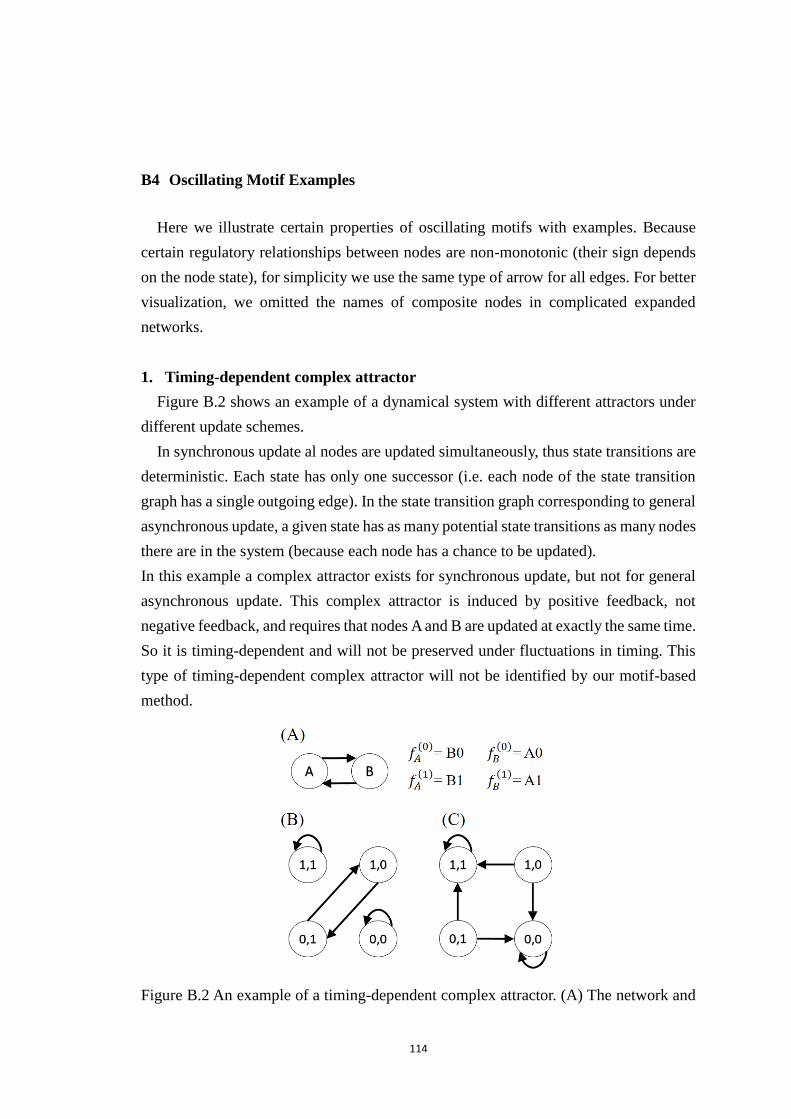
114

B4 Oscillating Motif Examples

Here we illustrate certain properties of oscillating motifs with examples. Because

certain regulatory relationships between nodes are non-monotonic (their sign depends

on the node state), for simplicity we use the same type of arrow for all edges. For better

visualization, we omitted the names of composite nodes in complicated expanded

networks.

1. Timing-dependent complex attractor

Figure B.2 shows an example of a dynamical system with different attractors under

different update schemes.

In synchronous update al nodes are updated simultaneously, thus state transitions are

deterministic. Each state has only one successor (i.e. each node of the state transition

graph has a single outgoing edge). In the state transition graph corresponding to general

asynchronous update, a given state has as many potential state transitions as many nodes

there are in the system (because each node has a chance to be updated).

In this example a complex attractor exists for synchronous update, but not for general

asynchronous update. This complex attractor is induced by positive feedback, not

negative feedback, and requires that nodes A and B are updated at exactly the same time.

So it is timing-dependent and will not be preserved under fluctuations in timing. This

type of timing-dependent complex attractor will not be identified by our motif-based

method.

Figure B.2 An example of a timing-dependent complex attractor. (A) The network and

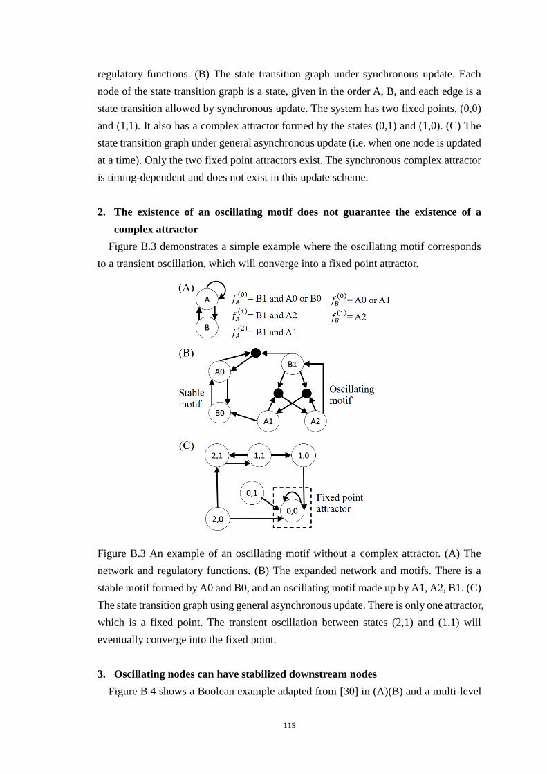
115

regulatory functions. (B) The state transition graph under synchronous update. Each

node of the state transition graph is a state, given in the order A, B, and each edge is a

state transition allowed by synchronous update. The system has two fixed points, (0,0)

and (1,1). It also has a complex attractor formed by the states (0,1) and (1,0). (C) The

state transition graph under general asynchronous update (i.e. when one node is updated

at a time). Only the two fixed point attractors exist. The synchronous complex attractor

is timing-dependent and does not exist in this update scheme.

2. The existence of an oscillating motif does not guarantee the existence of a

complex attractor

Figure B.3 demonstrates a simple example where the oscillating motif corresponds

to a transient oscillation, which will converge into a fixed point attractor.

Figure B.3 An example of an oscillating motif without a complex attractor. (A) The

network and regulatory functions. (B) The expanded network and motifs. There is a

stable motif formed by A0 and B0, and an oscillating motif made up by A1, A2, B1. (C)

The state transition graph using general asynchronous update. There is only one attractor,

which is a fixed point. The transient oscillation between states (2,1) and (1,1) will

eventually converge into the fixed point.

3. Oscillating nodes can have stabilized downstream nodes

Figure B.4 shows a Boolean example adapted from [30] in (A)(B) and a multi-level

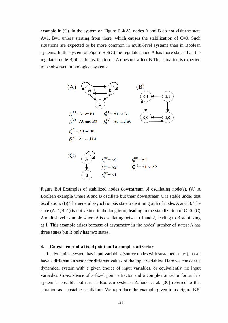
116

example in (C). In the system on Figure B.4(A), nodes A and B do not visit the state

A=1, B=1 unless starting from there, which causes the stabilization of C=0. Such

situations are expected to be more common in multi-level systems than in Boolean

systems. In the system of Figure B.4(C) the regulator node A has more states than the

regulated node B, thus the oscillation in A does not affect B This situation is expected

to be observed in biological systems.

Figure B.4 Examples of stabilized nodes downstream of oscillating node(s). (A) A

Boolean example where A and B oscillate but their downstream C is stable under that

oscillation. (B) The general asynchronous state transition graph of nodes A and B. The

state (A=1,B=1) is not visited in the long term, leading to the stabilization of C=0. (C)

A multi-level example where A is oscillating between 1 and 2, leading to B stabilizing

at 1. This example arises because of asymmetry in the nodes’ number of states: A has

three states but B only has two states.

4. Co-existence of a fixed point and a complex attractor

If a dynamical system has input variables (source nodes with sustained states), it can

have a different attractor for different values of the input variables. Here we consider a

dynamical system with a given choice of input variables, or equivalently, no input

variables. Co-existence of a fixed point attractor and a complex attractor for such a

system is possible but rare in Boolean systems. Zañudo et al. [30] referred to this

situation as unstable oscillation. We reproduce the example given in as Figure B.5.

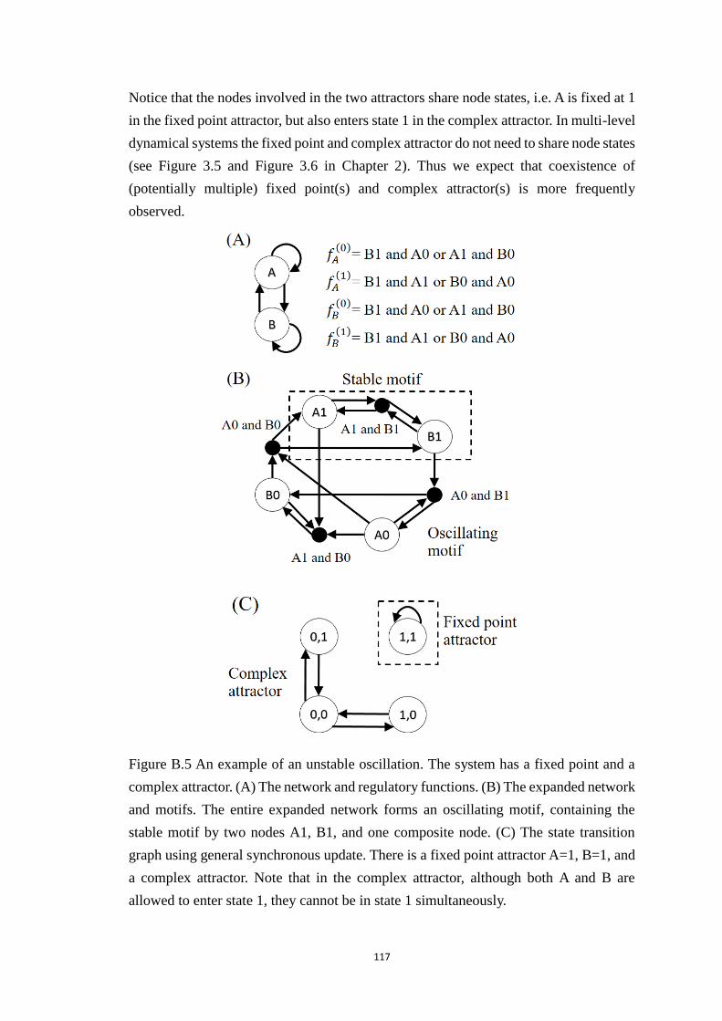
117

Notice that the nodes involved in the two attractors share node states, i.e. A is fixed at 1

in the fixed point attractor, but also enters state 1 in the complex attractor. In multi-level

dynamical systems the fixed point and complex attractor do not need to share node states

(see Figure 3.5 and Figure 3.6 in Chapter 2). Thus we expect that coexistence of

(potentially multiple) fixed point(s) and complex attractor(s) is more frequently

observed.

Figure B.5 An example of an unstable oscillation. The system has a fixed point and a

complex attractor. (A) The network and regulatory functions. (B) The expanded network

and motifs. The entire expanded network forms an oscillating motif, containing the

stable motif by two nodes A1, B1, and one composite node. (C) The state transition

graph using general synchronous update. There is a fixed point attractor A=1, B=1, and

a complex attractor. Note that in the complex attractor, although both A and B are

allowed to enter state 1, they cannot be in state 1 simultaneously.

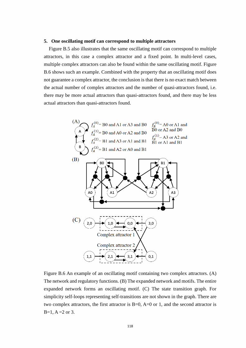
118

5. One oscillating motif can correspond to multiple attractors

Figure B.5 also illustrates that the same oscillating motif can correspond to multiple

attractors, in this case a complex attractor and a fixed point. In multi-level cases,

multiple complex attractors can also be found within the same oscillating motif. Figure

B.6 shows such an example. Combined with the property that an oscillating motif does

not guarantee a complex attractor, the conclusion is that there is no exact match between

the actual number of complex attractors and the number of quasi-attractors found, i.e.

there may be more actual attractors than quasi-attractors found, and there may be less

actual attractors than quasi-attractors found.

Figure B.6 An example of an oscillating motif containing two complex attractors. (A)

The network and regulatory functions. (B) The expanded network and motifs. The entire

expanded network forms an oscillating motif. (C) The state transition graph. For

simplicity self-loops representing self-transitions are not shown in the graph. There are

two complex attractors, the first attractor is B=0, A=0 or 1, and the second attractor is

B=1, A =2 or 3.

119

B5 Generation of regulatory functions in synthetic networks

Here we describe how we randomly generated regulatory functions among those

consistent with the number of regulators and number of states for each node.

In the network generation part, each node’s regulators are generated. In the

benchmarks, we generated networks where each node has two input nodes. For each

target node, we assign to each combination of different states of the regulator nodes a

randomly selected state of the target node. For example, if Boolean target node A is

regulated by Boolean nodes B and C, each of the four state combinations of B and C

will be randomly assigned to either the function of A0 or A1. Different input

combinations assigned to the same target state will be separated by an ‘or’ operator. For

example, combinations B0 C0 and B1 C0 are assigned to A0, then the function of A0 is

just fA(0) = (B0 and C0) or (B1 and C0). If at the end of the assignment a target state did

not get any assigned combination, this function is ineffective, and we discard all the

functions of this target node and start over to generate a new set of functions.

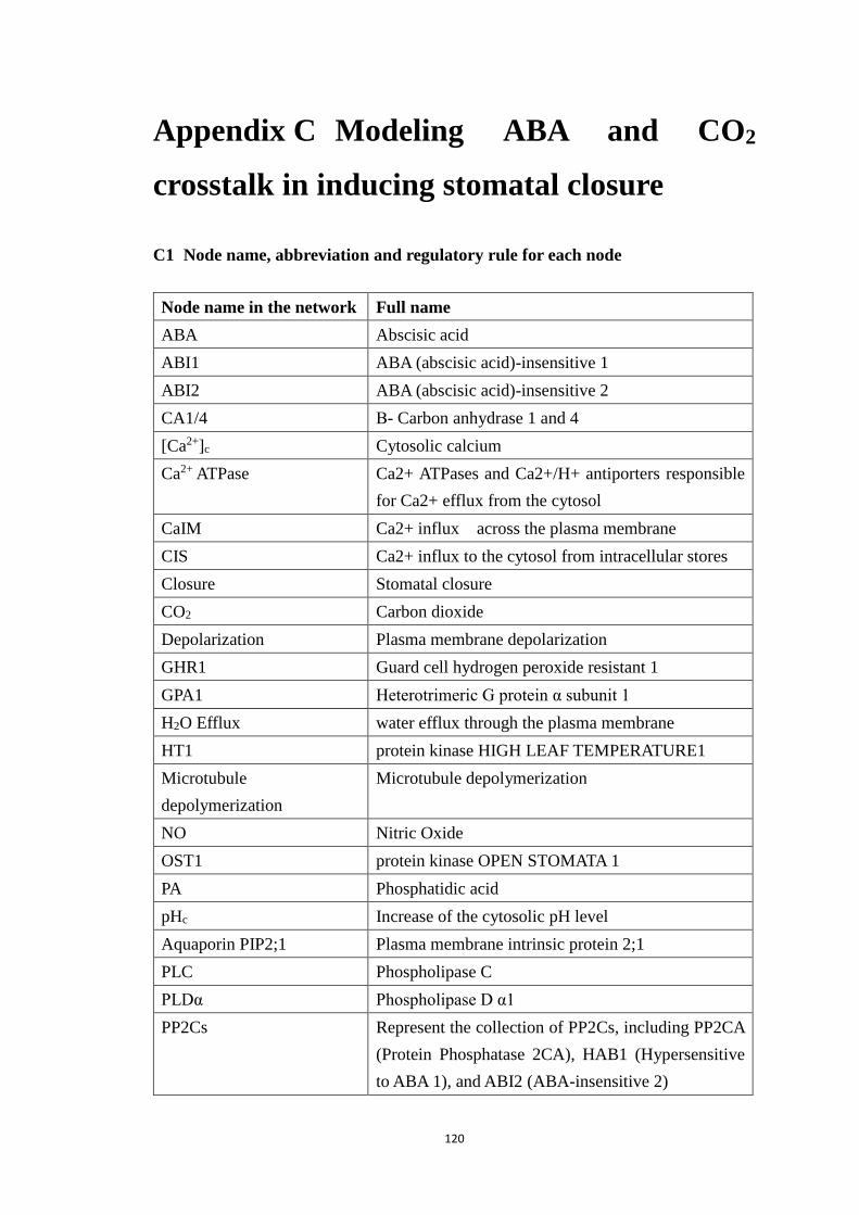
120

Appendix C Modeling ABA and CO2

crosstalk in inducing stomatal closure

C1 Node name, abbreviation and regulatory rule for each node

Node name in the network Full name

ABA Abscisic acid

ABI1 ABA (abscisic acid)-insensitive 1

ABI2 ABA (abscisic acid)-insensitive 2

CA1/4 Β- Carbon anhydrase 1 and 4

[Ca2+]c Cytosolic calcium

Ca2+ ATPase Ca2+ ATPases and Ca2+/H+ antiporters responsible

for Ca2+ efflux from the cytosol

CaIM Ca2+ influx across the plasma membrane

CIS Ca2+ influx to the cytosol from intracellular stores

Closure Stomatal closure

CO2 Carbon dioxide

Depolarization Plasma membrane depolarization

GHR1 Guard cell hydrogen peroxide resistant 1

GPA1 Heterotrimeric G protein α subunit 1

H2O Efflux water efflux through the plasma membrane

HT1 protein kinase HIGH LEAF TEMPERATURE1

Microtubule

depolymerization

Microtubule depolymerization

NO Nitric Oxide

OST1 protein kinase OPEN STOMATA 1

PA Phosphatidic acid

pHc Increase of the cytosolic pH level

Aquaporin PIP2;1 Plasma membrane intrinsic protein 2;1

PLC Phospholipase C

PLDα Phospholipase D α1

PP2Cs Represent the collection of PP2Cs, including PP2CA

(Protein Phosphatase 2CA), HAB1 (Hypersensitive

to ABA 1), and ABI2 (ABA-insensitive 2)

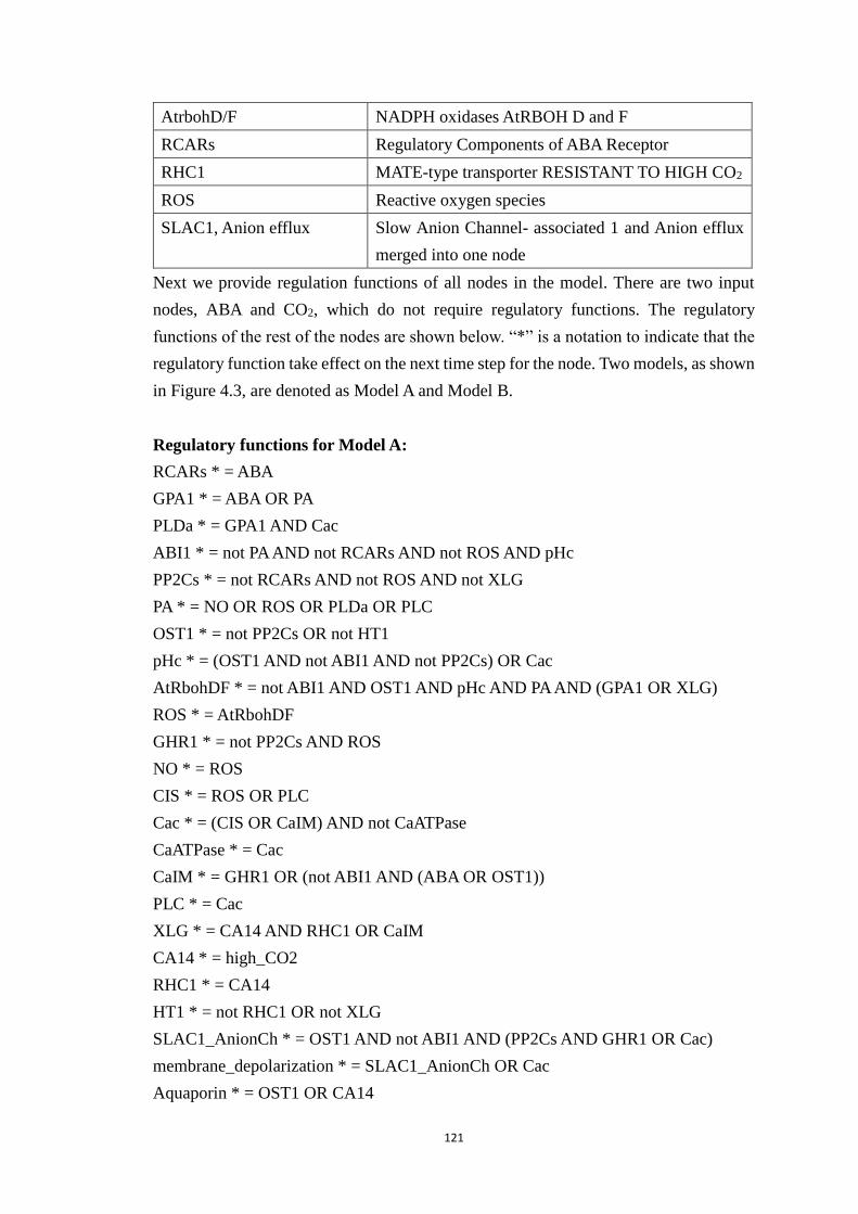
121

AtrbohD/F NADPH oxidases AtRBOH D and F

RCARs Regulatory Components of ABA Receptor

RHC1 MATE-type transporter RESISTANT TO HIGH CO2

ROS Reactive oxygen species

SLAC1, Anion efflux Slow Anion Channel- associated 1 and Anion efflux

merged into one node

Next we provide regulation functions of all nodes in the model. There are two input

nodes, ABA and CO2, which do not require regulatory functions. The regulatory

functions of the rest of the nodes are shown below. “*” is a notation to indicate that the

regulatory function take effect on the next time step for the node. Two models, as shown

in Figure 4.3, are denoted as Model A and Model B.

Regulatory functions for Model A:

RCARs * = ABA

GPA1 * = ABA OR PA

PLDa * = GPA1 AND Cac

ABI1 * = not PA AND not RCARs AND not ROS AND pHc

PP2Cs * = not RCARs AND not ROS AND not XLG

PA * = NO OR ROS OR PLDa OR PLC

OST1 * = not PP2Cs OR not HT1

pHc * = (OST1 AND not ABI1 AND not PP2Cs) OR Cac

AtRbohDF * = not ABI1 AND OST1 AND pHc AND PA AND (GPA1 OR XLG)

ROS * = AtRbohDF

GHR1 * = not PP2Cs AND ROS

NO * = ROS

CIS * = ROS OR PLC

Cac * = (CIS OR CaIM) AND not CaATPase

CaATPase * = Cac

CaIM * = GHR1 OR (not ABI1 AND (ABA OR OST1))

PLC * = Cac

XLG * = CA14 AND RHC1 OR CaIM

CA14 * = high_CO2

RHC1 * = CA14

HT1 * = not RHC1 OR not XLG

SLAC1_AnionCh * = OST1 AND not ABI1 AND (PP2Cs AND GHR1 OR Cac)

membrane_depolarization * = SLAC1_AnionCh OR Cac

Aquaporin * = OST1 OR CA14

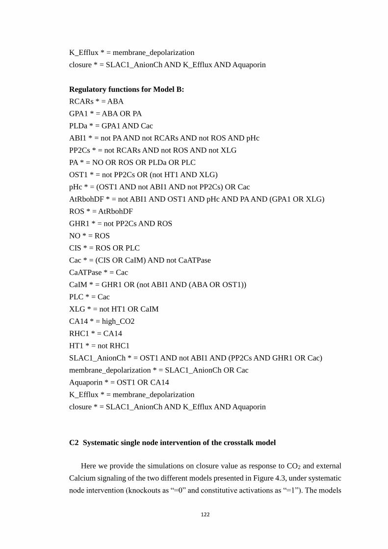
122

K_Efflux * = membrane_depolarization

closure * = SLAC1_AnionCh AND K_Efflux AND Aquaporin

Regulatory functions for Model B:

RCARs * = ABA

GPA1 * = ABA OR PA

PLDa * = GPA1 AND Cac

ABI1 * = not PA AND not RCARs AND not ROS AND pHc

PP2Cs * = not RCARs AND not ROS AND not XLG

PA * = NO OR ROS OR PLDa OR PLC

OST1 * = not PP2Cs OR (not HT1 AND XLG)

pHc * = (OST1 AND not ABI1 AND not PP2Cs) OR Cac

AtRbohDF * = not ABI1 AND OST1 AND pHc AND PA AND (GPA1 OR XLG)

ROS * = AtRbohDF

GHR1 * = not PP2Cs AND ROS

NO * = ROS

CIS * = ROS OR PLC

Cac * = (CIS OR CaIM) AND not CaATPase

CaATPase * = Cac

CaIM * = GHR1 OR (not ABI1 AND (ABA OR OST1))

PLC * = Cac

XLG * = not HT1 OR CaIM

CA14 * = high_CO2

RHC1 * = CA14

HT1 * = not RHC1

SLAC1_AnionCh * = OST1 AND not ABI1 AND (PP2Cs AND GHR1 OR Cac)

membrane_depolarization * = SLAC1_AnionCh OR Cac

Aquaporin * = OST1 OR CA14

K_Efflux * = membrane_depolarization

closure * = SLAC1_AnionCh AND K_Efflux AND Aquaporin

C2 Systematic single node intervention of the crosstalk model

Here we provide the simulations on closure value as response to CO2 and external

Calcium signaling of the two different models presented in Figure 4.3, under systematic

node intervention (knockouts as “=0” and constitutive activations as “=1”). The models

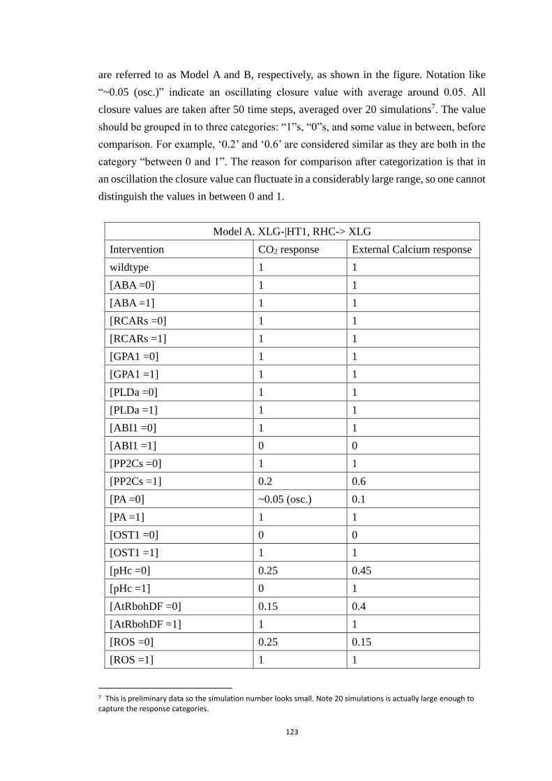
123

are referred to as Model A and B, respectively, as shown in the figure. Notation like

“~0.05 (osc.)” indicate an oscillating closure value with average around 0.05. All

closure values are taken after 50 time steps, averaged over 20 simulations7. The value

should be grouped in to three categories: “1”s, “0”s, and some value in between, before

comparison. For example, ‘0.2’ and ‘0.6’ are considered similar as they are both in the

category “between 0 and 1”. The reason for comparison after categorization is that in

an oscillation the closure value can fluctuate in a considerably large range, so one cannot

distinguish the values in between 0 and 1.

Model A. XLG-|HT1, RHC-> XLG

Intervention CO2 response External Calcium response

wildtype 1 1

[ABA =0] 1 1

[ABA =1] 1 1

[RCARs =0] 1 1

[RCARs =1] 1 1

[GPA1 =0] 1 1

[GPA1 =1] 1 1

[PLDa =0] 1 1

[PLDa =1] 1 1

[ABI1 =0] 1 1

[ABI1 =1] 0 0

[PP2Cs =0] 1 1

[PP2Cs =1] 0.2 0.6

[PA =0] ~0.05 (osc.) 0.1

[PA =1] 1 1

[OST1 =0] 0 0

[OST1 =1] 1 1

[pHc =0] 0.25 0.45

[pHc =1] 0 1

[AtRbohDF =0] 0.15 0.4

[AtRbohDF =1] 1 1

[ROS =0] 0.25 0.15

[ROS =1] 1 1

7 This is preliminary data so the simulation number looks small. Note 20 simulations is actually large enough to capture the response categories.

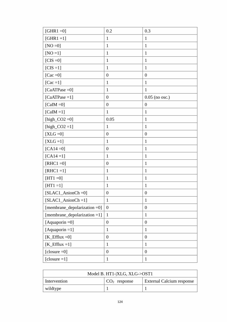
124

[GHR1 =0] 0.2 0.3

[GHR1 =1] 1 1

[NO =0] 1 1

[NO =1] 1 1

[CIS =0] 1 1

[CIS =1] 1 1

[Cac =0] 0 0

[Cac =1] 1 1

[CaATPase =0] 1 1

[CaATPase =1] 0 0.05 (no osc.)

[CaIM =0] 0 0

[CaIM =1] 1 1

[high_CO2 =0] 0.05 1

[high_CO2 =1] 1 1

[XLG =0] 0 0

[XLG =1] 1 1

[CA14 =0] 0 1

[CA14 =1] 1 1

[RHC1 =0] 0 1

[RHC1 =1] 1 1

[HT1 =0] 1 1

[HT1 =1] 1 1

[SLAC1_AnionCh =0] 0 0

[SLAC1_AnionCh =1] 1 1

[membrane_depolarization =0] 0 0

[membrane_depolarization =1] 1 1

[Aquaporin =0] 0 0

[Aquaporin =1] 1 1

[K_Efflux =0] 0 0

[K_Efflux =1] 1 1

[closure =0] 0 0

[closure =1] 1 1

Model B. HT1-|XLG, XLG->OST1

Intervention CO2 response External Calcium response

wildtype 1 1

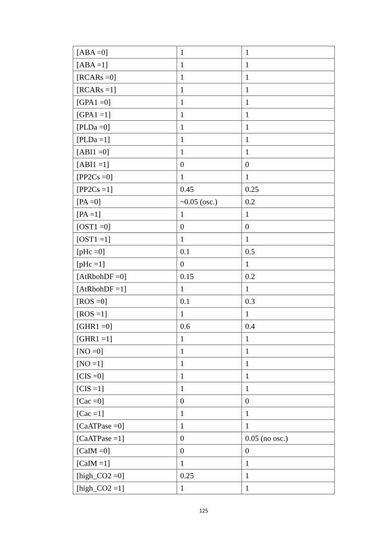
125

[ABA =0] 1 1

[ABA =1] 1 1

[RCARs =0] 1 1

[RCARs =1] 1 1

[GPA1 =0] 1 1

[GPA1 =1] 1 1

[PLDa =0] 1 1

[PLDa =1] 1 1

[ABI1 =0] 1 1

[ABI1 =1] 0 0

[PP2Cs =0] 1 1

[PP2Cs =1] 0.45 0.25

[PA =0] ~0.05 (osc.) 0.2

[PA =1] 1 1

[OST1 =0] 0 0

[OST1 =1] 1 1

[pHc =0] 0.1 0.5

[pHc =1] 0 1

[AtRbohDF =0] 0.15 0.2

[AtRbohDF =1] 1 1

[ROS =0] 0.1 0.3

[ROS =1] 1 1

[GHR1 =0] 0.6 0.4

[GHR1 =1] 1 1

[NO =0] 1 1

[NO =1] 1 1

[CIS =0] 1 1

[CIS =1] 1 1

[Cac =0] 0 0

[Cac =1] 1 1

[CaATPase =0] 1 1

[CaATPase =1] 0 0.05 (no osc.)

[CaIM =0] 0 0

[CaIM =1] 1 1

[high_CO2 =0] 0.25 1

[high_CO2 =1] 1 1

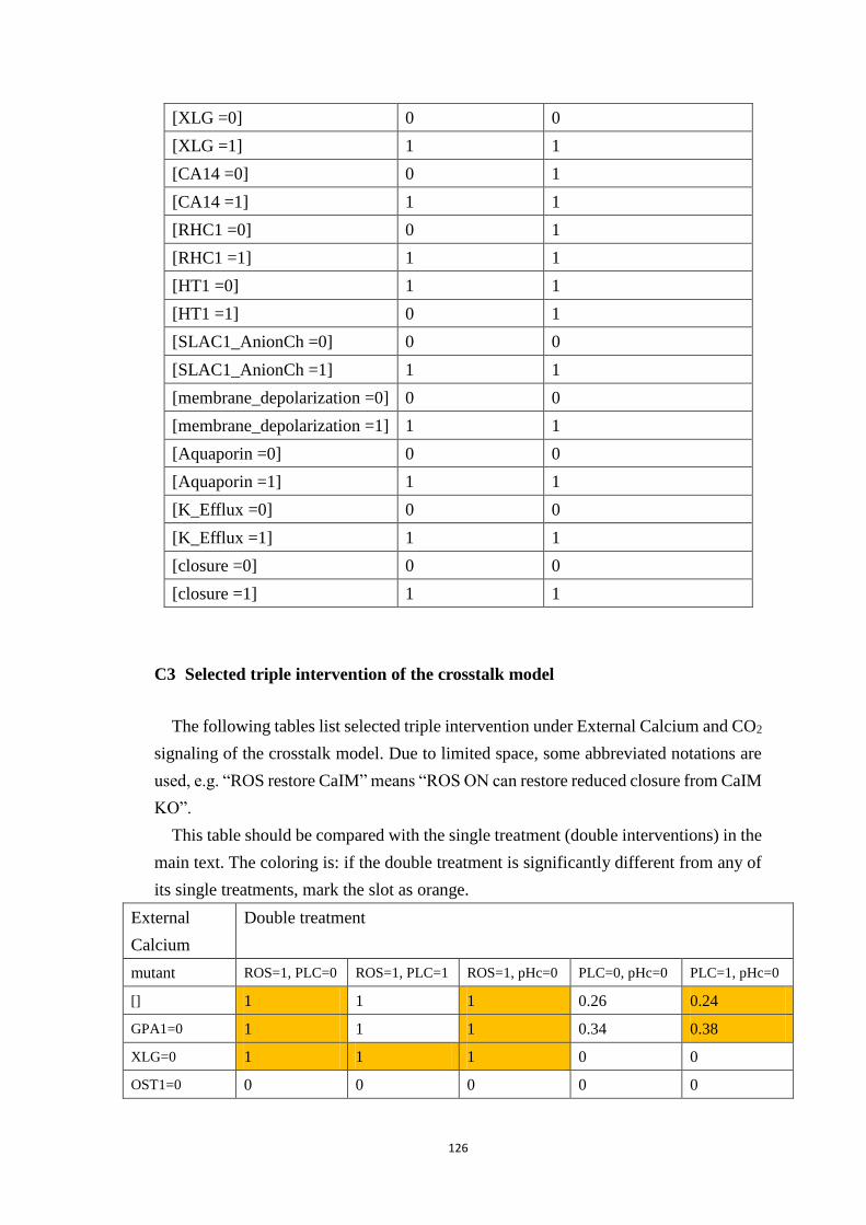
126

[XLG =0] 0 0

[XLG =1] 1 1

[CA14 =0] 0 1

[CA14 =1] 1 1

[RHC1 =0] 0 1

[RHC1 =1] 1 1

[HT1 =0] 1 1

[HT1 =1] 0 1

[SLAC1_AnionCh =0] 0 0

[SLAC1_AnionCh =1] 1 1

[membrane_depolarization =0] 0 0

[membrane_depolarization =1] 1 1

[Aquaporin =0] 0 0

[Aquaporin =1] 1 1

[K_Efflux =0] 0 0

[K_Efflux =1] 1 1

[closure =0] 0 0

[closure =1] 1 1

C3 Selected triple intervention of the crosstalk model

The following tables list selected triple intervention under External Calcium and CO2

signaling of the crosstalk model. Due to limited space, some abbreviated notations are

used, e.g. “ROS restore CaIM” means “ROS ON can restore reduced closure from CaIM

KO”.

This table should be compared with the single treatment (double interventions) in the

main text. The coloring is: if the double treatment is significantly different from any of

its single treatments, mark the slot as orange.

External

Calcium

Double treatment

mutant ROS=1, PLC=0 ROS=1, PLC=1 ROS=1, pHc=0 PLC=0, pHc=0 PLC=1, pHc=0

[] 1 1 1 0.26 0.24

GPA1=0 1 1 1 0.34 0.38

XLG=0 1 1 1 0 0

OST1=0 0 0 0 0 0

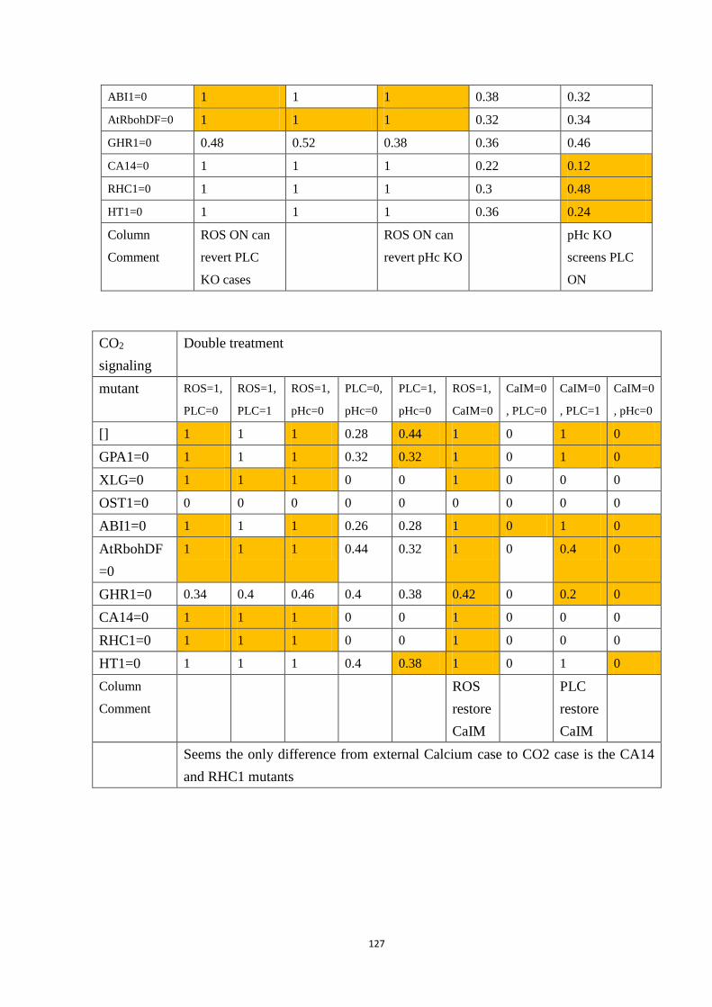
127

ABI1=0 1 1 1 0.38 0.32

AtRbohDF=0 1 1 1 0.32 0.34

GHR1=0 0.48 0.52 0.38 0.36 0.46

CA14=0 1 1 1 0.22 0.12

RHC1=0 1 1 1 0.3 0.48

HT1=0 1 1 1 0.36 0.24

Column

Comment

ROS ON can

revert PLC

KO cases

ROS ON can

revert pHc KO

pHc KO

screens PLC

ON

CO2

signaling

Double treatment

mutant ROS=1,

PLC=0

ROS=1,

PLC=1

ROS=1,

pHc=0

PLC=0,

pHc=0

PLC=1,

pHc=0

ROS=1,

CaIM=0

CaIM=0

, PLC=0

CaIM=0

, PLC=1

CaIM=0

, pHc=0

[] 1 1 1 0.28 0.44 1 0 1 0

GPA1=0 1 1 1 0.32 0.32 1 0 1 0

XLG=0 1 1 1 0 0 1 0 0 0

OST1=0 0 0 0 0 0 0 0 0 0

ABI1=0 1 1 1 0.26 0.28 1 0 1 0

AtRbohDF

=0

1 1 1 0.44 0.32 1 0 0.4 0

GHR1=0 0.34 0.4 0.46 0.4 0.38 0.42 0 0.2 0

CA14=0 1 1 1 0 0 1 0 0 0

RHC1=0 1 1 1 0 0 1 0 0 0

HT1=0 1 1 1 0.4 0.38 1 0 1 0

Column

Comment

ROS

restore

CaIM

PLC

restore

CaIM

Seems the only difference from external Calcium case to CO2 case is the CA14

and RHC1 mutants

128

References

1. Sun, Z., et al., Multi-level modeling of light-induced stomatal opening offers new insights into

its regulation by drought. PLoS Comput Biol, 2014. 10(11): p. e1003930.

2. Gan, X. and R. Albert, Analysis of a dynamic model of guard cell signaling reveals the stability

of signal propagation. BMC Systems Biology, 2016. 10(1): p. 78.

3. Thomas, R. and European Molecular Biology Organization., Kinetic logic : a Boolean approach

to the analysis of complex regulatory systems : proceedings of the EMBO course "Formal

analysis of genetic regulation," held in Brussels, September 6-16, 1977. Lecture notes in

biomathematics. 1979, Berlin ; New York: Springer-Verlag. xiii, 507 p.

4. Albert, R., et al., A new discrete dynamic model of ABA-induced stomatal closure predicts key

feedback loops. PLOS Biology, 2017. 15(9): p. e2003451.

5. Shannon, P., et al., Cytoscape: A Software Environment for Integrated Models of Biomolecular

Interaction Networks. Genome Research, 2003. 13(11): p. 2498-2504.

6. Hagberg, A.A., D.A. Schult, and P.J. Swart. Exploring network structure, dynamics, and function

using NetworkX. in Proceedings of the 7th Python in Science Conference (SciPy2008). 2008.

Pasadena, CA USA.

7. Morris, M.K., et al., Logic-based models for the analysis of cell signaling networks. Biochemistry,

2010. 49(15): p. 3216-24.

8. Abou-Jaoudé, W., et al., Logical Modeling and Dynamical Analysis of Cellular Networks.

Frontiers in Genetics, 2016. 7(94).

9. Wynn, M.L., et al., Logic-based models in systems biology: a predictive and parameter-free

network analysis method. Integr Biol (Camb), 2012. 4(11): p. 1323-37.

10. Laubenbacher, R., et al., Algebraic Models and Their Use in Systems Biology, in Discrete and

Topological Models in Molecular Biology, N. Jonoska and M. Saito, Editors. 2014, Springer Berlin

Heidelberg: Berlin, Heidelberg. p. 443-474.

11. Wang, R.S., A. Saadatpour, and R. Albert, Boolean modeling in systems biology: an overview of

methodology and applications. Phys Biol, 2012. 9.

12. Veliz-Cuba, A., A.S. Jarrah, and R. Laubenbacher, Polynomial algebra of discrete models in

systems biology. Bioinformatics, 2010. 26(13): p. 1637-43.

13. Saadatpour, A., R. Albert, and T.C. Reluga, A Reduction Method for Boolean Network Models

Proven to Conserve Attractors. SIAM J. Appl. Dyn. Syst., 2013. 12.

14. Naldi, A., et al., Dynamically consistent reduction of logical regulatory graphs. Theoretical

Computer Science, 2011. 412(21): p. 2207-2218.

15. Naldi, A., et al., Cooperative development of logical modelling standards and tools with

CoLoMoTo. Bioinformatics, 2015. 31(7): p. 1154-1159.

16. Chaouiya, C., et al., SBML qualitative models: a model representation format and infrastructure

to foster interactions between qualitative modelling formalisms and tools. BMC Syst Biol, 2013.

7: p. 135.

17. Helikar, T., et al., The Cell Collective: Toward an open and collaborative approach to systems

biology. BMC Systems Biology, 2012. 6(1): p. 96.

18. Chaouiya, C., A. Naldi, and D. Thieffry, Logical modelling of gene regulatory networks with

GINsim. Methods Mol Biol, 2012. 804: p. 463-79.

129

19. Albert, I., et al., Boolean network simulations for life scientists. Source Code for Biology and

Medicine, 2008. 3(1): p. 16.

20. Zheng, J., et al., SimBoolNet—a Cytoscape plugin for dynamic simulation of signaling networks.

Bioinformatics, 2010. 26(1): p. 141-142.

21. Müssel, C., M. Hopfensitz, and H.A. Kestler, BoolNet—an R package for generation,

reconstruction and analysis of Boolean networks. Bioinformatics, 2010. 26(10): p. 1378-1380.

22. Zhang, R., et al., Network model of survival signaling in large granular lymphocyte leukemia.

Proc Natl Acad Sci U S A, 2008. 105(42): p. 16308-13.

23. Saadatpour, A., et al., Dynamical and Structural Analysis of a T Cell Survival Network Identifies

Novel Candidate Therapeutic Targets for Large Granular Lymphocyte Leukemia. PLOS

Computational Biology, 2011. 7(11): p. e1002267.

24. Steinway, S.N., et al., Network modeling of TGFbeta signaling in hepatocellular carcinoma

epithelial-to-mesenchymal transition reveals joint sonic hedgehog and Wnt pathway activation.

Cancer Res, 2014. 74(21): p. 5963-77.

25. Steinway, S.N., et al., Combinatorial interventions inhibit TGFβ-driven epithelial-to-

mesenchymal transition and support hybrid cellular phenotypes. 2015. 1: p. 15014.

26. Remy, E., P. Ruet, and D. Thieffry, Graphic requirements for multistability and attractive cycles

in a Boolean dynamical framework. Advances in Applied Mathematics, 2008. 41(3): p. 335-350.

27. Richard, A. and J.-P. Comet, Necessary conditions for multistationarity in discrete dynamical

systems. Discrete Applied Mathematics, 2007. 155(18): p. 2403-2413.

28. Richard, A., Negative circuits and sustained oscillations in asynchronous automata networks.

Advances in Applied Mathematics, 2010. 44(4): p. 378-392.

29. Wang, R.-S. and R. Albert, Elementary signaling modes predict the essentiality of signal

transduction network components. BMC Systems Biology, 2011. 5(1): p. 44.

30. Zanudo, J.G. and R. Albert, An effective network reduction approach to find the dynamical

repertoire of discrete dynamic networks. Chaos, 2013. 23.

31. Zanudo, J.G. and R. Albert, Cell fate reprogramming by control of intracellular network dynamics.

PLoS Comput Biol, 2015. 11(4): p. e1004193.

32. Sun, Z. and R. Albert, Node-independent elementary signaling modes: A measure of redundancy

in Boolean signaling transduction networks. Network Science, 2016. 4(3): p. 273-292.

33. Gan, X. and R. Albert, General method to find the attractors of discrete dynamic models of

biological systems. Phys Rev E, 2018. 97(4-1): p. 042308.

34. Maheshwari, P. and R. Albert, A framework to find the logic backbone of a biological network.

BMC Systems Biology, 2017. 11(1): p. 122.

35. Stigler, B. and H.M. Chamberlin, A regulatory network modeled from wild-type gene expression

data guides functional predictions in Caenorhabditis elegans development. BMC Syst Biol, 2012.

6.

36. Chifman, J., et al., The core control system of intracellular iron homeostasis: a mathematical

model. J Theor Biol, 2012. 300: p. 91-9.

37. Massague, J., TGF-beta signal transduction. Annu Rev Biochem, 1998. 67.

38. Xu, H.L., et al., Construction and Validation of a Regulatory Network for Pluripotency and Self-

Renewal of Mouse Embryonic Stem Cells. Plos Computational Biology, 2014. 10(8).

39. Kestler, H.A., et al., Network modeling of signal transduction: establishing the global view.

Bioessays, 2008. 30(11-12): p. 1110-25.

130

40. Tyson, J.J., K. Chen, and B. Novak, Network dynamics and cell physiology. Nature Reviews

Molecular Cell Biology, 2001. 2(12): p. 908-916.

41. Kauffman, S.A., Metabolic stability and epigenesis in randomly constructed genetic nets. J Theor

Biol, 1969. 22.

42. Glass, L. and S.A. Kauffman, Logical analysis of continuous, nonlinear biochemical control

networks. J Theor Biol, 1973. 39.

43. Miskov-Zivanov, N., et al., The duration of T cell stimulation is a critical determinant of cell fate

and plasticity. Sci Signal, 2013. 6(300): p. ra97.

44. Deritei, D., et al., Principles of dynamical modularity in biological regulatory networks. Sci Rep,

2016. 6: p. 21957.

45. Murrugarra, D. and R. Laubenbacher, Regulatory patterns in molecular interaction networks. J

Theor Biol, 2011. 288.

46. Li, S., S.M. Assmann, and R. Albert, Predicting essential components of signal transduction

networks: a dynamic model of guard cell abscisic acid signaling. PLoS Biol, 2006. 4(10): p. e312.

47. Schroeder, J.I., et al., Guard Cell Signal Transduction. Annu Rev Plant Physiol Plant Mol Biol,

2001. 52: p. 627-658.

48. Shimazaki, K., et al., Light regulation of stomatal movement. Annu Rev Plant Biol, 2007. 58: p.

219-47.

49. Assmann, S.M., Enhancement of the Stomatal Response to Blue Light by Red Light, Reduced

Intercellular Concentrations of CO(2), and Low Vapor Pressure Differences. Plant Physiol, 1988.

87.

50. Bergmann, D.C. and F.D. Sack, Stomatal development. Annu Rev Plant Biol, 2007. 58.

51. MacArthur, B.D., A. Ma'ayan, and I.R. Lemischka, Systems biology of stem cell fate and cellular

reprogramming. Nature Reviews Molecular Cell Biology, 2009. 10(10): p. 672-681.

52. Ansotegui, C. and F. Manya, Mapping problems with finite-domain variables to problems with

Boolean variables. Theory Appl of Satisfiability Test, 2005. 3542.

53. Van Ham, P., How to deal with more than two levels, in Kinetic logic : a Boolean approach to the

analysis of complex regulatory systems : proceedings of the EMBO course "Formal analysis of

genetic regulation," held in Brussels, September 6-16, 1977, R. Thomas, Editor. 1979, Springer-

Verlag: Berlin ; New York. p. 326-344.

54. Didier, G., E. Remy, and C. Chaouiya, Mapping multivalued onto Boolean dynamics. J Theor Biol,

2011. 270.

55. Karlsson, P.E., Blue light regulation of stomata in wheat seedlings. I. Influence of red background

illumination and initial conductance level. Physiologia Plantarum, 1986. 66: p. 5.

56. Veliz-Cuba, A., et al., Steady state analysis of Boolean molecular network models via model

reduction and computational algebra. BMC Bioinformatics, 2014. 15(1): p. 221.

57. Remy, E. and P. Ruet, On differentiation and homeostatic behaviours of Boolean dynamical

systems. Lecture Notes in Bioinformatics, 2007. 4780: p. 92-101.

58. Liu, Y.-Y., J.-J. Slotine, and A.-L. Barabasi, Controllability of complex networks. Nature, 2011.

473(7346): p. 167-173.

59. Lin, C.T., STRUCTURAL CONTROLLABILITY. Ieee Transactions on Automatic Control, 1974.

AC19(3): p. 201-208.

60. Mochizuki, A., et al., Dynamics and control at feedback vertex sets. II: A faithful monitor to

determine the diversity of molecular activities in regulatory networks. Journal of Theoretical

131

Biology, 2013. 335: p. 130-146.

61. Schwartz, A., et al., Anion-Channel Blockers Inhibit S-Type Anion Channels and Abscisic Acid

Responses in Guard Cells. Plant Physiol, 1995. 109(2): p. 651-658.

62. Kim, T.H., et al., Guard cell signal transduction network: advances in understanding abscisic acid,

CO2, and Ca2+ signaling. Annu Rev Plant Biol, 2010. 61: p. 561-91.

63. Arenas, A., et al., Synchronization in complex networks. Physics Reports, 2008. 469(3): p. 93-

153.

64. Tian, X.-J., et al., Achieving diverse and monoallelic olfactory receptor selection through dual-

objective optimization design. Proceedings of the National Academy of Sciences, 2016. 113(21):

p. E2889-E2898.

65. Barabasi, A.-L. and Z.N. Oltvai, Network biology: understanding the cell's functional

organization. Nat Rev Genet, 2004. 5(2): p. 101-113.

66. Albert, R. and R.S. Wang, DISCRETE DYNAMIC MODELING OF CELLULAR SIGNALING NETWORKS,

in Methods in Enzymology: Computer Methods, Part B, M.L. Johnson and L. Brand, Editors. 2009,

Elsevier Academic Press Inc: San Diego. p. 281-306.

67. Pennisi, M., et al., A methodological approach for using high-level Petri Nets to model the

immune system response. BMC Bioinformatics, 2016. 17(19): p. 498.

68. Butchy, A.A. and N. Miskov-Zivanov, Discrete modeling of macrophage differentiation. The

Journal of Immunology, 2017. 198(1 Supplement): p. 67.13-67.13.

69. Albert, R. and J. Thakar, Boolean modeling: a logic-based dynamic approach for understanding

signaling and regulatory networks and for making useful predictions. Wiley Interdiscip Rev Syst

Biol Med, 2014. 6(5): p. 353-69.

70. Li, F., et al., The yeast cell-cycle network is robustly designed. Proceedings of the National

Academy of Sciences of the United States of America, 2004. 101(14): p. 4781-4786.

71. Abou-Jaoude, W., et al., Logical Modeling and Dynamical Analysis of Cellular Networks. Front

Genet, 2016. 7: p. 94.

72. Havlin, S., et al., Challenges in network science: Applications to infrastructures, climate, social

systems and economics. The European Physical Journal Special Topics, 2012. 214(1): p. 273-293.

73. Onnela, J.-P., et al., Structure and tie strengths in mobile communication networks. Proceedings

of the National Academy of Sciences, 2007. 104(18): p. 7332-7336.

74. Federico, B., P. Matjaž, and L. Vito, Determinants of public cooperation in multiplex networks.

New Journal of Physics, 2017. 19(7): p. 073017.

75. Lancichinetti, A., S. Fortunato, and J. Kertész, Detecting the overlapping and hierarchical

community structure in complex networks. New Journal of Physics, 2009. 11(3): p. 033015.

76. Mori, F. and A. Mochizuki, Expected Number of Fixed Points in Boolean Networks with Arbitrary

Topology. Physical Review Letters, 2017. 119(2): p. 028301.

77. Klarner, H., A. Bockmayr, and H. Siebert, Computing maximal and minimal trap spaces of

Boolean networks. Natural Computing, 2015. 14(4): p. 535-544.

78. Garg, A., et al., Synchronous versus asynchronous modeling of gene regulatory networks.

Bioinformatics, 2008. 24(17): p. 1917-1925.

79. Naldi, A., D. Thieffry, and C. Chaouiya, Decision Diagrams for the Representation and Analysis

of Logical Models of Genetic Networks, in Computational Methods in Systems Biology:

International Conference CMSB 2007, Edinburgh, Scotland, September 20-21, 2007.

Proceedings, M. Calder and S. Gilmore, Editors. 2007, Springer Berlin Heidelberg: Berlin,

132

Heidelberg. p. 233-247.

80. Traynard, P., et al., Logical model specification aided by model-checking techniques: application

to the mammalian cell cycle regulation. Bioinformatics, 2016. 32(17): p. i772-i780.

81. Gómez Tejeda Zañudo, J., M. Scaltriti, and R. Albert, A network modeling approach to elucidate

drug resistance mechanisms and predict combinatorial drug treatments in breast cancer.

Cancer Convergence, 2017. 1(1): p. 5.

82. Chifman, J., et al., Activated Oncogenic Pathway Modifies Iron Network in Breast Epithelial Cells:

A Dynamic Modeling Perspective. PLOS Computational Biology, 2017. 13(2): p. e1005352.

83. Dubrova, E., M. Liu, and M. Teslenko, Finding Attractors in Synchronous Multiple-Valued

Networks Using SAT-based Bounded Model Checking. Journal of Multiple-Valued Logic and Soft

Computing, 2012. 19(1-3): p. 109-131.

84. Hinkelmann, F., et al., ADAM: Analysis of Discrete Models of Biological Systems Using Computer

Algebra. BMC Bioinformatics, 2011. 12(1): p. 295.

85. Puniya, B.L., et al., Systems Perturbation Analysis of a Large-Scale Signal Transduction Model

Reveals Potentially Influential Candidates for Cancer Therapeutics. Frontiers in Bioengineering

and Biotechnology, 2016. 4: p. 10.

86. Cheng, X., M. Sun, and J.E.S. Socolar, Autonomous Boolean modelling of developmental gene

regulatory networks. Journal of the Royal Society Interface, 2013. 10(78): p. 20120574.

87. Murrugarra, D., et al., Modeling stochasticity and variability in gene regulatory networks.

EURASIP Journal on Bioinformatics and Systems Biology, 2012. 2012(1): p. 5.

88. Chaves, M., R. Albert, and E.D. Sontag, Robustness and fragility of Boolean models for genetic

regulatory networks. J Theor Biol, 2005. 235(3): p. 431-49.

89. Thomas, R., Regulatory networks seen as asynchronous automata: A logical description. Journal

of Theoretical Biology, 1991. 153(1): p. 1-23.

90. Saadatpour, A., I. Albert, and R. Albert, Attractor analysis of asynchronous Boolean models of

signal transduction networks. J Theor Biol, 2010. 266(4): p. 641-56.

91. Klemm, K. and S. Bornholdt, Topology of biological networks and reliability of information

processing. Proceedings of the National Academy of Sciences of the United States of America,

2005. 102(51): p. 18414-18419.

92. Gan, X. and R. Albert. A general method to find the attractors of discrete dynamic models of

biological systems. in the 8th International Conference on Physics and Control (PhysCon 2017).

2017. Florence, Italy.

93. Brown, F.M., The Blake Canonical Form, in Boolean Reasoning: The Logic of Boolean Equations.

1990, Springer US: Boston, MA. p. 71-86.

94. Quine, W.V., The Problem of Simplifying Truth Functions. The American Mathematical Monthly,

1952. 59(8): p. 521-531.

95. Quine, W.V., A Way to Simplify Truth Functions. The American Mathematical Monthly, 1955.

62(9): p. 627-631.

96. McCluskey, E.J., Minimization of Boolean Functions*. Bell System Technical Journal, 1956. 35(6):

p. 1417-1444.

97. Aldana, M., S. Coppersmith, and L.P. Kadanoff, Boolean Dynamics with Random Couplings, in

Perspectives and Problems in Nolinear Science: A Celebratory Volume in Honor of Lawrence

Sirovich, E. Kaplan, J.E. Marsden, and K.R. Sreenivasan, Editors. 2003, Springer New York: New

York, NY. p. 23-89.

133

98. Wang, R.S. and R. Albert, Effects of community structure on the dynamics of random threshold

networks. Physical Review E, 2013. 87(1).

99. Berenguier, D., et al., Dynamical modeling and analysis of large cellular regulatory networks.

Chaos, 2013. 23(2): p. 025114.

100. Reisig, W., Petri Nets, in Modeling in Systems Biology: The Petri Net Approach, I. Koch, W. Reisig,

and F. Schreiber, Editors. 2011, Springer London: London. p. 37-56.

101. Chaouiya, C., et al., Petri net representation of multi-valued logical regulatory graphs. Natural

Computing, 2011. 10(2): p. 727-750.

102. Samaga, R. and S. Klamt, Modeling approaches for qualitative and semi-quantitative analysis

of cellular signaling networks. Cell Communication and Signaling, 2013. 11(1): p. 43.

103. Johnson, D.B., Finding All the Elementary Circuits of a Directed Graph. SIAM Journal on

Computing, 1975. 4(1): p. 77-84.

104. Assmann, S.M. and T. Jegla, Guard cell sensory systems: recent insights on stomatal responses

to light, abscisic acid, and CO2. Current Opinion in Plant Biology, 2016. 33: p. 157-167.

105. Munemasa, S., et al., Mechanisms of abscisic acid-mediated control of stomatal aperture.

Current Opinion in Plant Biology, 2015. 28: p. 154-162.

106. Davies, W.J. and M.J. Bennett, Achieving more crop per drop. Nature Plants, 2015. 1: p. 15118.

107. Roelfsema, M.R. and H. Kollist, Tiny pores with a global impact. New Phytol, 2013. 197(1): p.

11-5.

108. Acharya, B.R. and S.M. Assmann, Hormone interactions in stomatal function. Plant Mol Biol,

2009. 69(4): p. 451-62.

109. Li, J., et al., Regulation of Abscisic Acid-Induced Stomatal Closure and Anion Channels by Guard

Cell AAPK Kinase. Science, 2000. 287(5451): p. 300-303.

110. Zhang, W., L.-M. Fan, and W.-H. Wu, Osmo-sensitive and stretch-activated calcium-permeable

channels in Vicia faba guard cells are regulated by actin dynamics. Plant physiology, 2007.

143(3): p. 1140-1151.

111. Jiang, K., et al., The ARP2/3 complex mediates guard cell actin reorganization and stomatal

movement in Arabidopsis. The Plant cell, 2012. 24(5): p. 2031-2040.

112. Engineer, C.B., et al., CO2 Sensing and CO2 Regulation of Stomatal Conductance: Advances and

Open Questions. Trends in plant science, 2016. 21(1): p. 16-30.

113. Brearley, J., M.A. Venis, and M.R. Blatt, The effect of elevated CO2 concentrations on K+ and

anion channels of Vicia faba L. guard cells. Planta, 1997. 203: p. 10.

114. ASSMANN, S.M., The cellular basis of guard cell sensing of rising CO2. Plant, Cell & Environment,

1999. 22(6): p. 629-637.

115. Hu, H., et al., Carbonic anhydrases are upstream regulators of CO2-controlled stomatal

movements in guard cells. Nature cell biology, 2010. 12(1): p. 87-18.

116. Tian, W., et al., A molecular pathway for CO(2) response in Arabidopsis guard cells. Nat Commun,

2015. 6: p. 6057.

117. Hõrak, H., et al., A Dominant Mutation in the HT1 Kinase Uncovers Roles of MAP Kinases and

GHR1 in CO₂-Induced Stomatal Closure. The Plant Cell, 2016. 28(10): p. 2493-2509.

118. Hsu, P.-K., et al., Abscisic acid-independent stomatal CO₂ signal transduction

pathway and convergence of CO₂ and ABA signaling downstream of OST1 kinase.

Proceedings of the National Academy of Sciences, 2018. 115(42): p. E9971-E9980.

119. Chakravorty, D. and S.M. Assmann, G protein subunit phosphorylation as a regulatory

134

mechanism in heterotrimeric G protein signaling in mammals, yeast, and plants. Biochemical

Journal, 2018. 475(21): p. 3331-3357.

120. Mishra, G., et al., A Bifurcating Pathway Directs Abscisic Acid Effects on Stomatal Closure and

Opening in <em>Arabidopsis</em>. Science, 2006. 312(5771): p. 264-266.

121. Lee, Y.-R.J. and S.M. Assmann, Arabidopsis thaliana ‘extra-large GTP-binding protein’ (AtXLG1):

a new class of G-protein. Plant Molecular Biology, 1999. 40(1): p. 55-64.

122. Ding, L., S. Pandey, and S.M. Assmann, Arabidopsis extra-large G proteins (XLGs) regulate root

morphogenesis. Plant J, 2008. 53(2): p. 248-63.

123. Pandey, S., et al., Regulation of root-wave response by extra large and conventional G proteins

in Arabidopsis thaliana. Plant J, 2008. 55(2): p. 311-22.

124. Chakravorty, D., et al., Extra-Large G Proteins Expand the Repertoire of Subunits in Arabidopsis

Heterotrimeric G Protein Signaling. Plant Physiol, 2015. 169(1): p. 512-29.

125. Pandey, S., et al., G-protein complex mutants are hypersensitive to abscisic acid regulation of

germination and postgermination development. Plant Physiol, 2006. 141(1): p. 243-56.

126. Urano, D., et al., Saltational evolution of the heterotrimeric G protein signaling mechanisms in

the plant kingdom. Sci Signal, 2016. 9(446): p. ra93.

127. Maruta, N., et al., Membrane-localized extra-large G proteins and Gbg of the heterotrimeric G

proteins form functional complexes engaged in plant immunity in Arabidopsis. Plant Physiol,

2015. 167(3): p. 1004-16.

128. Wang, X.Q., et al., G protein regulation of ion channels and abscisic acid signaling in Arabidopsis

guard cells. Science, 2001. 292(5524): p. 2070-2.

129. Ge, X.M., et al., Heterotrimeric G protein mediates ethylene-induced stomatal closure via

hydrogen peroxide synthesis in Arabidopsis. Plant J, 2015. 82(1): p. 138-50.

130. Jones, A.M. and S.M. Assmann, Plants: the latest model system for G-protein research. EMBO

Rep, 2004. 5(6): p. 572-8.

131. Wu, W.H. and S.M. Assmann, A membrane-delimited pathway of G-protein regulation of the

guard-cell inward K+ channel. Proc Natl Acad Sci U S A, 1994. 91(14): p. 6310-4.

132. Coursol, S., et al., Sphingolipid signalling in Arabidopsis guard cells involves heterotrimeric G

proteins. Nature, 2003. 423(6940): p. 651-4.

133. Li, J.H., et al., A signaling pathway linking nitric oxide production to heterotrimeric G protein

and hydrogen peroxide regulates extracellular calmodulin induction of stomatal closure in

Arabidopsis. Plant Physiol, 2009. 150(1): p. 114-24.

134. Albert, R., et al., A new discrete dynamic model of ABA-induced stomatal closure predicts key

feedback loops. PLoS Biol, 2017. 15(9): p. e2003451.

135. Chater, C., et al., Elevated CO2-Induced Responses in Stomata Require ABA and ABA Signaling.

Curr Biol, 2015. 25(20): p. 2709-16.

136. Clapham, D.E., Calcium signaling. Cell, 1995. 80(2): p. 259-268.

137. BROADLEY, M.R. and P.J. WHITE, Calcium in Plants. Annals of Botany, 2003. 92(4): p. 487-511.

138. Allen, G.J., et al., A defined range of guard cell calcium oscillation parameters encodes stomatal

movements. Nature, 2001. 411: p. 1053.

139. Hashimoto, M., et al., Arabidopsis HT1 kinase controls stomatal movements in response to CO2.

Nature Cell Biology, 2006. 8: p. 391.

140. Rozum, J.C. and R. Albert, Identifying (un)controllable dynamical behavior in complex networks.

PLOS Computational Biology, 2018. 14(12): p. e1006630.

135

141. Lawson, T., et al., Mesophyll photosynthesis and guard cell metabolism impacts on stomatal

behaviour. New Phytologist, 2014. 203(4): p. 1064-1081.

142. MOTT, K.A., Opinion: Stomatal responses to light and CO2 depend on the mesophyll. Plant, Cell

& Environment, 2009. 32(11): p. 1479-1486.

143. Fujita, T., K. Noguchi, and I. Terashima, Apoplastic mesophyll signals induce rapid stomatal

responses to CO2 in Commelina communis. New Phytologist, 2013. 199(2): p. 395-406.

144. Wong, S.C., I.R. Cowan, and G.D. Farquhar, Stomatal conductance correlates with

photosynthetic capacity. Nature, 1979. 282(5737): p. 424-426.

145. McAdam, S.A.M. and T.J. Brodribb, Mesophyll Cells Are the Main Site of Abscisic Acid

Biosynthesis in Water-Stressed Leaves. Plant Physiology, 2018. 177(3): p. 911-917.

146. Tõldsepp, K., et al., Mitogen-activated protein kinases MPK4 and MPK12 are key components

mediating CO2-induced stomatal movements. The Plant Journal, 2018. 96(5): p. 1018-1035.

147. Mustilli, A.C., et al., Arabidopsis OST1 protein kinase mediates the regulation of stomatal

aperture by abscisic acid and acts upstream of reactive oxygen species production. Plant Cell,

2002. 14(12): p. 3089-99.

148. Albert, R. and H.G. Othmer, The topology of the regulatory interactions predicts the expression

pattern of the segment polarity genes in Drosophila melanogaster. J Theor Biol, 2003. 223.

149. Yuan, Z., et al., Exact controllability of complex networks. Nature Communications, 2013. 4: p.

2447.

150. Zañudo, J.G.T., G. Yang, and R. Albert, Structure-based control of complex networks with

nonlinear dynamics. Proceedings of the National Academy of Sciences, 2017. 114(28): p. 7234-

7239.

151. Yang, G., J. Gomez Tejeda Zanudo, and R. Albert, Target Control in Logical Models Using the

Domain of Influence of Nodes. bioRxiv, 2018.

152. K. Chandra, A. and G. Markowsky, On the number of prime implicants. Vol. 24. 1978. 7-11.

Vita

Xiao Gan

Education and Research:

The Pennsylvania State University University Park, USA.

Ph.D. Major: Physics Aug. 2013 – Aug. 2019 (expected)

Advisor: Prof. Réka Albert

National Laboratory of Solid State Microstructures, Nanjing University,

Research assistant Jun. 2012 – Jun. 2013

Advisor: Prof. Xinglong Wu

Nanjing University, Kuang Yaming Honors School Nanjing, China

Bachelor of Science, Major: Physics Aug. 2018 - Jun. 2012

Publications

Gan, X and Albert, R. "Modeling biological information processing networks." In Physics of

Molecular and Cellular Systems, Krastan B. Blagoev and Herbert Levine (eds.) (Invited book

chapter, submitted for publication).

Gan, X and Albert, R. "General method to find the attractors of discrete dynamic models of

biological systems." Physical Review E 97(4): 042308 (2018).

Gan, X and Albert, R. "A general method to find the attractors of discrete dynamic models of

biological systems." Presented at the 8th International Conference on Physics and Control, Florence,

Italy, July 2017, Proceedings paper available at: http://lib.physcon.ru/doc?id=f916c9044267

Gan, X and Albert, R "Analysis of a dynamic model of guard cell signaling reveals the stability of

signal propagation." BMC Systems Biology 10.1 (2016): 78.

Shan, Y., Wu, X., Gan, X., et al. “CdS: Mn–Polysulfido Complex Nanoclusters with H2O2-

Dependent and Site-Specific Color Changes” The Journal of Physical Chemistry C, 118(20),

pp.11085-11092. (2014)

Gan, Z., Xiong, S., Wu, X., Xu, T., Zhu, X., Gan, X., et al. “Mechanism of photoluminescence from

chemically derived graphene oxide: role of chemical reduction.” Advanced Optical Materials, 1(12),

926-932. (2013)

Jiang J., Zhu H., Zhou Y. GAN X., et al. "Research on diffraction of twisted nematic liquid crystal",

Physics Experimentation, 31, No.10, 44-46 (2011)

HONORS AND AWARDS

The Downsbrough Department Head's Chair in Physics (fellowship) in 2019

Financial support for invited talk in Shenzhen Institutes of Advanced Technology (SIAT), Chinese

Academy of Science (2018)

Financial support for NetSciX, Hangzhou, China (2018)

The Downsbrough Graduate Fellowship in Physics, Pennsylvania State University (2017)

NSF travel award for ICSB (International Conference on Systems Biology), Virginia Tech (2017)

The David C. Duncan Graduate Fellowship in Physics, Pennsylvania State University (2016)

The People’s Scholarship - Special Award, Nanjing University (2010)

The People’s Scholarship, Nanjing University (2009 & 2010)