1

Understanding the Decline of The Western Alaskan

Steller Sea Lion: Assessing the Evidence Concerning

Multiple Hypothesis

Prepared by

MRAG Americas, Inc.

Tampa, Florida

For

NOAA Fisheries

Alaska Fisheries Science Center

Seattle, Washington

#AB133F-02-CN-0085:

MRAG Americas, Inc.

110 South Hoover Boulevard

Suite 212

Tampa, FL 33609

Authors: Nicholas Wolf and Marc Mangel

2

Executive Summary

Although millions of dollars have been spent exploring the cause, and a wide variety of

hypotheses have been proposed, the precipitous decline of the western population of

Steller sea lions (Eumatopias jubatus) since the late 1970’s has proven to be very

difficult to explain. We view this as an opportunity for ecological detection, a process in

which multiple hypotheses simultaneously compete and their success is arbitrated by the

relevant data. The authors of a recent comprehensive review of the problem emphasized

repeatedly that the system is in dire need of a modeling approach that takes advantage of

the data available at small spatial scales (at the level of the rookery). Our approach is

designed to do just that.

We begin by summarizing the biology of the Steller sea lion, including life history, prey

base and relevant fisheries, and other marine mammals. The various competing

hypotheses can be viewed in the context of different food webs of increasing complexity.

For the case of Steller sea lions, there exist sufficient data to explore the following ten

hypotheses:

H1: Total prey availability affects fecundity;

H2: Total prey availability affects pup recruitment;

H3: Total prey availability affects non-pup survival;

H4: Pollock fraction in the environment affects fecundity;

H5: Pollock fraction in the environment affects pup recruitment;

3

H6: Pollock fraction in the environment affects non-pup survival;

H7: Fishery activity affects pup recruitment;

H8: Fishery activity affects non-pup survival;

H9: Harbor seal density (predation) affects pup recruitment;

H10: Harbor seal density (predation) affects non-pup survival

We review a variety of previous studies, each of which has provided valuable insight

into the problem. However, none made use of both spatial and temporal variation in sea

lion counts as well as the environmental data. Most of the researchers pooled data across

space, combining all rookery censuses within each year and performing their analyses

using a composite time series representing the entire western population; and the

remainder of the researchers effectively pooled data across time, fitting a single trend line

to all the census data from each rookery.

We assembled, organized, and analyzed or re-analyzed databases at the spatial scale of

the rookery and on an annual time scale concerning:

• Counts of sea lion pups and non-pups in various censuses of rookeries over the

past 25 years;

• Commercial fisheries (both foreign and domestic) effort;

• The NMFS triennial trawl survey for the major prey species of Steller sea lions;

• Harbor seal counts (used as a proxy, via diet breadth theory, for the predation

pressure from killer whales).

4

We obtained counts of Steller sea lions from the NMFS/AFSC/NMML online database.

We assume that fisheries and survey haul data corresponding to locations within a 300-

km foraging radius from a sea lion rookery are relevant to that rookery. We included

eleven taxa that were described as “dominant,” “important,” or “most common” prey

types in a review of Steller sea lion diet studies in the 2001 SSL restricted areas SEIS.

We calculated estimates of fishing activity in minutes per year from the NMFS

groundfish fishery observer database. Our estimates of harbor seal density came from

online NMFS/AFSC marine mammal stock assessments and reports, a Marine Mammal

Commission report, and eight journal articles. We developed new methods (space-time

plots) for presenting the relevant data.

Pup counts should be fairly accurate, because pups are almost always on land during the

summer surveys. Thus, in common with previous investigators, we use a sighting

probability of 1 for pups. In contrast, the number of non-pups counted in any rookery

census is nearly always smaller than the true number of individuals associated with the

site, because an unknown fraction of the non-pups were at sea at the time of counting. To

account for observation error in the counts of non-pups, we extended the traditional beta-

binomial model for simultaneous estimation of the two parameters of a binomial

distribution to account for the situation of summer censuses for non-pups. In particular,

we assume that the probability of sighting in a given census is drawn from a beta density

and that the number of observed animals follows a binomial distribution determined by

the true number of non-pups present and the beta-distributed probability of sighting. We

used data from rookeries that were censused multiple times within a single year to

5

calibrate the parameters in our observation error distribution. We estimate a mean

sighting probability of about 60%.

To account for process uncertainty, we use a stochastic population model in which vital

rates (non-pup fecundity and survival, pup survival) are functions of the local conditions

determined by the abundance of food, the fraction of food that is pollock, the level of

fishing activity, and the abundance of harbor seals. The local conditions modify base

values of fecundity and survival. Each of the functions involving local conditions

contains one unknown parameter, and we design these function in such a way that a value

of the parameter equal to 0 means that the associated hypotheses has no effect on the

population dynamics. We assume a Holling type III functional response for the

relationship between local total prey availability and each vital rate, a power function for

the relationship between local pollock fraction and vital rates, an exponential function for

the relationship between minutes of local fishery activity and survival rates, and a knife-

edge step function (as in standard diet selection theory) for the relationship between local

harbor seal abundance (killer whale predation index) and survival rates.

We estimate the unknown parameters by comparing the predictions of the stochastic

population model with the observed counts. To do this, we start with the beta-binomial

observation error distribution and a two-life-stage stochastic population model employing

the local vital rates and calculate the probability of observing the sequence of reported

pup and non-pup counts at a particular rookery, given (1) relevant local conditions and

(2) a particular set of parameter values in the hypothesized equations. We find this

6

probability using backwards iteration and by “thinking along sample paths,” adapting the

method of path integration used in physics. Analogous probabilities are calculated for all

rookeries and censuses and multiplied together to estimate the likelihood of the data

given the hypotheses and a particular set of parameter values. We compute the maximum

likelihood estimate (MLE) of each parameter and construct 10 one-dimensional profile

likelihoods so that we can examine the support for each parameter, holding the others at

their maximum likelihood estimates. For each parameter, we compute a profile

likelihood interval by finding the area under the curve that contains 95% or 99% of the

total area.

We consider that the data provide strong evidence for a hypothesis if the MLE of the

parameter associated with that hypothesis is non-zero and the profile likelihood interval

does not include 0. The data provide weak evidence for a hypothesis if the MLE of the

parameter associated with that hypothesis is non-zero but the profile likelihood interval

includes 0. If the MLE is 0, the data provide no evidence for the hypothesis.

Furthermore, we will classify the effects as strong effect, weak effect, or no effect,

depending upon how the MLE value of the parameter affects the predicted population

dynamics of Steller sea lions.

7

Our conclusions can be summarized in the following table:

Strong Evidence Weak Evidence No Evidence

Strong Effect H1: Total prey

availability affects

fecundity

H5: Pollock

fraction affects pup

recruitment

Moderate Effect H10: Harbor seal

density (predation)

affects non-pup

survival

Weak or No Effect H4: Pollock

fraction affects

fecundity

H2: Total prey

availability affects

pup recruitment

H3: Total prey

availability affects

non-pup survival

H6: Pollock

fraction affects non-

pup survival

H7: Fishery activity

affects pup

recruitment

H8: Fishery activity

affects non-pup

survival

H9: Harbor seal

density (predation)

affects pup

recruitment

Virtually all of the AIC weight (98.7%) is assigned to models with {H1, H4, H5, H10}

or {H1, H5, H10} and the difference between these two models, hypothesis H4, is about

5%. These results are not unexpected (indeed, each of the 10 hypotheses is plausible and

has been proposed at some point, with associated supporting data). What our work has

8

done is to guide the weight of the evidence, when all plausible hypotheses are competing,

towards those that win the competition.

We compare non-pup census data to the results of forward simulations based on different

model configurations for three rookeries in the western population and one in the eastern

population (as a control). Such simulations are analogous to controlled laboratory

experiments. Although both effects are statistically important, the effect of pollock on

recruitment is stronger than the effect of total prey on fecundity in the sense that the slope

of the predicted decline is much steeper in the case of pollock affecting recruitment.

Thus, the answer to the oft-asked question “Is it food” is yes and that it is both quality

and quantity of food. The more recent question “Is it killer whale predation” can be

answered too – sometimes, if harbor seal populations are sufficiently low, but not with a

large reduction in survival.

Our results suggest a natural framework for adaptive management in which one

designates the areas around some of the rookeries as experimental zones in which to

make fishery quotas contingent upon the results of pre-fishing season survey trawls. The

experimental treatments could be as follows:

• Rookeries around which fishing is not affected by the pre-season survey

information (control type 1).

• Rookeries around which no fishing occurs (control type 2)

9

• Rookeries around which fishing is reduced or prohibited if the total prey

biomass in the pre-season zone is below a critical threshold (which can be

determined using the model we developed).

• Rookeries around which a directed pollock fishery occurs if the pre-season

survey suggests that the fraction of pollock is above a critical threshold.

Our results also suggest a form of “adaptive observation”: Identify rookeries with high

numbers and low numbers of harbor seals (regardless of the number of sea lions). The

prediction of H10 is that the per-capita attack rate of killer whales on sea lions will be

much higher around rookeries where harbor seals are low. The alternative would occur,

for example, if H10 is false and environments that are bad for harbor seals are also bad

for sea lions, and vice versa. In such a case, the prediction is that there will be no

difference in the per capita rate of attack of killer whales.

10

1. Introduction: The Decline of Steller Sea Lions and The Method of

Multiple Hypotheses

The precipitous decline of the western population of Steller sea lions (Eumatopias

jubatus) since the late 1970’s has proven to be very difficult to explain. A significant

problem is that most aspects of the population and the environmental variables proposed

to explain its decline involve a combination of high spatial and temporal variability and

limited data availability. As a result, researchers who have attempted to model the

system have been forced to pool data across rookeries or across time, obscuring spatial

and/or temporal patterns (compare Figures 1.1 and 1.2). An additional complication

stems from the suggestion that the first decline in the 1980’s and the continued decline in

the 1990’s may have had very different causes. Specifically, much of the evidence seems

to point toward a “bottom-up” (food-related) problem in the initial decline and a “top-

down” (predation or other mortality-related) control since 1989 or so, although even

these general conclusions are contentious. This variation can be seen if one computes

annual mortality rates based on non-pup counts (Figure 1.3).

The authors of a recent comprehensive review of the problem (NRC 2003) emphasized

repeatedly that the system is in dire need of a modeling approach that takes advantage of

the data available at small spatial scales. Our approach is designed to do just that. In

this section, we give a broad overview of the biology of the organism (to ensure that our

models have the correct assumptions) and frame the general approach. We begin

(Section 1.1) with a review of the biology of the Steller sea lion that is relevant to the

11

modeling which we undertake here. We describe the fisheries with which the sea lions

may interact (and thus their prey base). We then summarize the problem (Section 1.2) as

one of competing hypotheses (mechanisms) that could explain the decline. Previous

work by MRAG Americas helps frame the issues that must be addressed. We then

(Section 1.3) explain the role of ecological detection (Hilborn and Mangel 1997) in

understanding this particular problem. In contrast to traditional single-hypothesis

statistical approaches, ecological detection is based on the notion of simultaneous

competition among multiple hypotheses, with relative strength assigned to each

hypothesis according to its ability to reproduce the data. Thus, in Section 1.4 we explain

the various hypotheses that we investigate here and in Section 1.5 explain how previous

studies have approached the problem.

Equipped with this background, we then (Section 2) describe the data that we acquired

and how we treated those data in preparation for analysis. In Section 3, we describe the

summarized versions of the data that underlie our work. We introduce the idea of space-

time plots of the data, where space is indexed by rookeries. Such plots of the data

immediately illuminate interesting aspects of the problem. The summarized data are

available at the web site given in Section 3.

Our models involve both process uncertainty and observation error. The latter is

introduced during summer counts of sea lions because, although all pups should be

visible on the beach, some non-pups may be at sea foraging during the time of the survey.

However, the sighting probability is also unknown. The problem of simultaneously

12

estimating the number of trials and the probability of success in a binomial process is an

exceptionally difficult one (Hilborn and Mangel 1997). The best existing solution is still

the beta-binomial model (Martz and Waller 1982; Evans et al 2000), in which the

sighting probability is assumed to follow a beta probability density and, conditioned on

that, the number of animals observed is binomially distributed with unknown true number

of animals and beta-distributed sighting probability. However, even the best existing

work was insufficient for our needs, so we have extended it appropriately in Section 4.

In Section 5, we introduce the vital rates that underlie our analysis. These are the

probabilities of annual non-pup survival and reproductive success and the probability that

a pup successfully recruits to the non-pup population. We also introduce the notion of

local conditions; that is, we assume that the vital rates depend upon the local conditions

within typical foraging range of a rookery. Then, in Section 6 we use a population model

with vital rates determined by local conditions to connect the hypotheses and data. We

adopt a method used in physics (path integration) to help us sort through the different

hypotheses about the cause of the decline; hence we call this the method of thinking

along sample paths.

In Section 6, we describe the details involved in computing likelihood to estimate

parameter values, and in Section 7 we present the results. In Section 8, we provide a

broad discussion about the implications of our work. In the Appendix, we explain what

the next steps in this work might be.

13

1.1 The Steller Sea Lion

The Steller sea lion, Eumatopias jubatus, occupies the north Pacific coastline from

central California to Japan. Evidence from mitochondrial DNA shows that the

population east of 144° W longitude is genetically distinct from the population west of

that line (Bickham et al. 1998), and an analysis of resightings of marked individuals

confirms that there is very little exchange of breeding individuals between the two

regions. Females tend to return either to their natal rookery (about 67% of the time in the

western stock) or to a neighboring rookery (Raum-Suryan et al. 2002). Thus, the set of

rookeries within each region qualifies as a metapopulation (York et al. 1996), a group of

local populations linked by dispersal (Hanski 2000), although our models have no

explicit migration parameter.

Rookeries are generally located on small, remote islands. Most pups (one per pregnant

female) are born within a two-month period centered in June (Pitcher et al. 2002), and

enter the water for the first time when they are 2-4 weeks old (Sandegren 1970). Mothers

alternate between nursing on land and foraging at sea, leaving the pups behind to fend for

themselves for 1-2 days at a time (NRC 2003). Pups depend on their mothers for

nourishment throughout most the first year, during which time they gradually learn to

forage and become proficient at diving. Dive depth increases from 70 m at 6 months of

age to 140 m at 12 months (Rehberg et al. 2001). Most pups wean by the end of their

first year, but a few nurse for a second year (Trites and Porter 2002; Pitcher and Calkins

1981).

14

The sex ratio at birth is approximately 50/50. Sexual maturity for females usually occurs

at around 4.5 years (Harmon 2001, Holmes and York 2003), but females as young as 3

years old have been observed with pups (Raum-Suryan et al. 2002).

After they wean, but before they become proficient at deep diving and catching fast-

swimming fish, pups may rely heavily upon slow-moving, easily captured prey, including

shrimp (Hansen 1997) or crab (P. Dayton, pers. comm..) The abundance of such prey

species could be important in determining the recruitment success of pups (Merrick and

Loughlin 1997).

Mature sea lions typically dive to depths of 250 m or less (Merrick and Loughlin 1997) in

search of their prey, which are mostly various kinds of groundfish. Time-depth recorder

studies indicate that much of the foraging time is spent near the bottom (Merrick et al.

1994). Therefore, the shallower parts of the continental shelf, where the water is less

than about 200 m deep, are generally assumed to be the most important foraging areas

(e.g. Gerber and Van Blaricom 2001).

Steller sea lions are largely opportunistic foragers keying in on locally and temporally

aggregated prey (including Walleye pollock, herring, eulachon, salmon and Pacific cod),

although they may display some prey preference under certain conditions. Walleye

pollock (Theragra chalcogramma) are currently the principal diet component for both the

Western stock and the stocks in the Eastern Aleutians and southeast Alaska (Anderson

and Blackburn 2002; Alverson 1992). Other important prey species include Atka

15

mackerel (Pleurogrammus monopterygius), Pacific cod (Gadus macrocephalus), and

Pacific herring (Clupea pallasi).

Walleye pollock, Atka mackerel, and Pacific cod are harvested primarily using

groundfish trawling gear. The largest groundfish harvests in the area occur in the Bering

Sea. The peak catch was more than 2.1 million mt (metric tons) in 1972, followed by a

decline in the late 1970’s and a recovery in the mid-1980’s. Total annual groundfish

catch since about 1985 has hovered near 1.5 million mt. Pollock comprise the vast

majority (over 76%) of the groundfish caught in the Bering Sea (NRC 2003). In the Gulf

of Alaska, there was a major peak in the pollock catch between 1976 and 1985, when up

to 300,000 mt per year were taken from the Shelikof Strait, between Kodiak Island and

the mainland. Catch restrictions limited the Shelikof Strait fishery to about 80,000 mt

starting in 1986, and total groundfish catch in the Gulf of Alaska has hovered around

200,000 mt per year since then (NRC 2003). Another fishery for groundfish developed in

the Aleutian Islands in the late 1970’s. Total annual catch grew slowly to about 180,000

mt between 1989 and 1996, dominated first by a pollock boom in the eastern Aleutians

and later by a peak in Atka mackerel. The pollock fishery declined to 24,000 mt per year

by 1998, when it was closed as a precautionary measure to protect the sea lions (NRC

2003).

Herring in Alaskan waters are currently harvested for their roe, using gillnets and purse

seines. Catch effort in this fishery is closely associated with known spawning locations

and timed to just precede the spawning period. A record catch of over 140,000 mt in

16

1970 declined to about 30,000 mt by the late 1970’s and remained at approximately that

level through the late 1990’s, with most of the harvest occurring in the eastern Bering

Sea. Catches have declined sharply since about 1997, resulting in closures of the fishery

in Prince William Sound and Cook Inlet (NRC 2003).

The Steller sea lion decline in western Alaska was preceded by declines in the

populations of Northern fur seals, Callorhinus ursinus, and Pacific harbor seals, Phoca

vitulina, occupying the same region. The causes of these declines remain similarly

unexplained (Merrick 1997). One possibility is the killer whale diet breadth hypothesis:

The range of the sea lions’ western population is also home to a large population of Killer

whales, Orcinus orca. Of these, a substantial number (certainly more than 100) belong to

the “transient” race (Barrett-Lennard et al. 1995), whose diet consists mainly of marine

mammals, including Steller sea lions (Matkin et al. 2002). Unfortunately, very little is

known about the spatial or temporal distribution of these whales. But if killer whales

expand and contract their diets in an adaptive manner, then the abundance of alternative

food sources (i.e. other marine mammals) may determine the magnitude of killer whale

predation on Steller sea lions at local scales (Mangel and Wolf, submitted). This

mechanism has recently received considerable attention (Springer et al 2003; Wade et al

2003). Our work allows one to separate plausibility and evidential weight in support of

this and all other hypotheses considered.

17

1.2 Summary of the Problem

While estimates of the eastern population of Steller sea lions have been growing slowly

since survey methods were standardized in the 1970’s, the estimates of the size of the

western population have fallen by more than 80%. The decline appears to have begun in

the eastern Aleutians and spread in both directions from there. The initial decline was

characterized by a loss of about 15% of the population per year (Figure 1.3),

accompanied by reduced size-at-age and other symptoms of nutritional stress (Calkins et

al. 1998; Castellini 1993). After 1989 or so, the rate of decline slowed to about 5% per

year (Sease and Loughlin 1999), and the available evidence suggests that animals in the

western population were actually in better condition than those in the growing eastern

population (Andrews et al. 2002). The western stock was listed as Endangered in 1997.

Numerous competing hypotheses have been proposed to explain the decline of the

western population. We explore these in more detail in subsequent sections and

consider a subset of hypotheses for which sufficient data are available to apply

appropriate analytical and statistical methods. Our approach is to compare the

hypotheses using ecological detection (Hilborn and Mangel 1997), in which alternative

models are confronted with the data and ranked according to their ability to produce it.

From the outset, we do not subscribe to a particular hypothesis and set out to support our

idea. Rather, we seek to understand the role of multiple mechanisms in the decline of the

Steller sea lion.

18

The various competing hypotheses can be viewed in the context of a series of

increasingly complicated food webs (MRAG Americas 2002). For example, the simplest

model for the interactions between marine mammals and a fishery is shown in Figure

1.4a. In this case, the target fish are assumed to be prey for both the fishery and marine

mammals. The interactions can be either indirect and thus bottom up, with the fishery

removing prey that the mammals or birds would otherwise take, or else direct, and thus

top-down, with incidental mortality of mammals or birds occurring during fishing

operations. This food web is one used implicitly when changes in marine mammals or

birds are assumed to be caused by fishery activities.

While Figure 1.4a may be a useful conceptual tool for framing interactions, it is overly

simplified. Potential complexities of the primary interactions include:

• age-specific factors in the interactions between major species;

• temporal and spatial components to the interactions; and

• availability of target species.

These complexities are included in the food web in Figure 1.4b. The trophic level

labeled “mammals and birds” makes no distinction between different life history stages,

such as juveniles and adults. Both the direct and indirect effects of the fishery may differ

between juveniles and adults, for a variety of reasons. Similarly, once this trophic level is

separated into adults and juveniles, effects on growth (especially the transition from

juvenile to adult) and reproduction (the production of new juveniles) may be different.

19

In addition, the simple web in Figure 1.4a is based on the assumption that the fishery

targets a single stock that is also the sole prey source for the marine mammals and birds.

However, marine mammals and birds often have cosmopolitan diets; thus the trophic

level occupied by “target fish” may also be occupied by other fish species that are

competitors of the target species and prey for the mammals and birds. In a similar way,

the marine mammals and birds may themselves be prey for other marine organisms, such

as toothed whales or sharks or marine diseases. These ideas are also captured in Figure

1.4b.

One should expect variation in ecosystems. Thus, the target species may be removed by

the fishery (leading to interference competition with the marine mammals or birds), but it

may also move in space relative to the location of the fishery and the marine mammals or

birds. Although the enlarged food web in Figure 1.4b is more complex, it ignores

environmental factors that affect the production of fish stocks. These factors may be

biotic (e.g. the level of zooplankton or primary production) or abiotic (e.g. different

temperature regimes). Figure 1.4c captures these ideas.

1.3 The Role of Ecological Detection

Each of the food webs in Figure 1.4 can be viewed as a pictorial model for the ecosystem

and its interactions. Now confronted with the information that Steller sea lions have

declined, different hypotheses could be generated by these models. We show some

examples in Table 1.1, knowing that these are “nested” in the sense that more than one of

them could apply.

20

Given a set of data concerning the decline of Steller sea lions, one view of the role of

analysis is that its purpose is to confront each of these putative mechanisms of the decline

with the data and allow the data to arbitrate between the different models. Hilborn and

Mangel (1997) call this process ecological detection. Ecological detection recognizes

that our understanding of the world will always be incomplete and that the goal should be

to achieve the best understanding possible by working with multiple competing

hypotheses and allowing the data to arbitrate the competition.

1.4 The Hypotheses

Numerous competing hypotheses have been proposed to explain the decline of the

western population (Ferrero and Fritz 2002). We will consider a subset of hypotheses for

which sufficient data are available to apply appropriate analytical and statistical methods.

H1-H3: Acute Nutritional Stress (Food Limitation) hypotheses

Fecundity (H1), pup recruitment (H2), or non-pup survival probability (H3) is a positive

function of the local encounter rate with groundfish prey. Specifically, starvation (H2,

H3) or termination of pregnancy (H1) occurs if an animal experiences a long series of

unsuccessful foraging attempts and fails to find enough to eat.

The motivation for these hypotheses is as follows. Prey availability is assumed to affect

body condition. Under poor foraging conditions, animals may lose condition because

they consume less prey, spend more time and energy hunting, or both. Body condition,

21

in turn, is known to be a significant determinant of the probability that a pregnant female

Steller sea lion actually completes her pregnancy and produces a pup (Pitcher et al.

1998). Poor foraging conditions also increase the probability of starvation and expose the

animals to additional predation risk during any extra time spent foraging, leading to

elevated mortality rates. The probability of pup recruitment may be linked indirectly to

prey availability if mothers are more likely to abandon pups under poor foraging

conditions, or it may be linked directly if starvation is a serious concern when the

inexperienced pups begin foraging for themselves near the end of their first year.

H4-H6: Chronic Nutritional Stress (Junk-food) hypotheses

Fecundity (H4), pup recruitment (H5), or non-pup survival probability (H6) is a positive

function of the fraction of prey other than Walleye pollock in the environment.

Specifically, starvation (H5, H6) or termination of pregnancy (H4) occur with higher

probability where prey other than pollock are relatively scarce.

There is general agreement that high fractions of pollock in the environment correlate

with poor performance by Steller sea lions, although the mechanism is still unclear.

Some versions of the mechanism call for the sea lions to suffer ill effects from shifting

their diet to consume too much pollock when it is abundant, while other versions propose

that the sea lions do not shift their diet but rather starve because there is not enough of

something other than pollock. We discuss several possibilities here, although our current

model does not specify the exact mechanism.

22

The idea that a pollock-intensive diet might lead to poor body condition and depressed

vital rates was first proposed by Alverson (1992) and supported by evidence showing a

strong inverse correlation between diet diversity and population decline rate across

rookeries (Merrick et al. 1997). Pollock do not contain as much fat as other prey species

(Rosen and Trites 2000, 2002), and Rosen and Trites (2000) found that captive Steller sea

lions lost weight on a pollock-only diet, even when fed ad-libitum.

Alternative mechanisms involve pups. For example, the limited dive depth and lack of

experience of pups probably restricts them to a subset of easily caught prey that might be

more difficult to find in environments where pollock dominate. Another possibility is

that the stomachs of pups may be too small to ingest enough calories if their diet is

composed primarily of pollock. Thus, pup recruitment probability may be especially

sensitive to prey species composition, and in particular it might be negatively correlated

with relative pollock abundance.

The approach that we develop is effective regardless of the particular mechanism as long

as one agrees that a larger fraction of pollock in the environment is not good for Steller

sea lions (i.e., the negative effect may derive either from too much pollock in the

environment or else from too little of something else; and pollock consumption may be

bad for the animals or it may have no effect).

23

H7, H8: Anthropogenic Activity (Fishery-related mortality) hypotheses

Survival probability of pups (H7) or non-pups (H8) is a declining function of the local

encounter rate with groundfish trawling operations.

The motivation for these hypotheses is as follows. Incidental mortality, usually resulting

from the entanglement of sea lions in fishing gear, was recently estimated to be killing

less than 100 animals per year now (Perez and Loughlin 1991; Loughlin and York 2002),

but at certain times and in certain places (e.g. the Shelikov Strait trawl fishery in the late

1970’s and early 1980’s) it was much higher (NRC 2003). Deliberate shooting of sea

lions by fishers may be another significant source of mortality, although its magnitude is

not well known. It was legal to shoot sea lions in defense of gear until 1990, and there

are anecdotal reports suggesting that shooting (even unrelated to defense of gear) may

still occur (NRC 2003). It may be very difficult to determine whether incidental or

deliberate mortality is the problem, since both might scale with fishing effort. However,

it seems likely that entanglement would be a bigger problem for naïve pups (Loughlin et

al. 1983), whereas adults are more likely to be targeted by shooters.

It is possible, of course, that fishing activity depletes food sources so that the effect of

fisheries is felt not directly (as in H7 or H8) but indirectly (as in H1-H3).

H9, H10: Predation mortality hypotheses

Survival probability of sea lions declines when local harbor seal density falls below a

critical threshold.

24

The motivation for this hypothesis is as follows. Not all Killer whales eat marine

mammals, but members of the transient race do. Steller sea lions in particular may

comprise 5-20% of their diet (Matkin et al. 2002). The stomach of one Killer whale that

washed up on a beach in British Columbia contained flipper tags from 14 different Steller

sea lion pups, all of which had been tagged at the Marmot Island rookery 3-4 years before

(Saulitis et al. 2000). If the transient Killer whale population is stable (as suggested by

Barrett-Lennard et al. 1995), but its more profitable prey types (in the sense of classical

diet choice theory) are being depleted (as suggested by Estes et al. 1998), then (according

to the optimal prey switching argument) Killer whale predation upon sea lions is thus

predicted to be more intense at sea lion rookeries around which there are few harbor

seals. A form of this hypothesis was proposed by Hanna (1922) to account for ‘missing’

fur seals. In Section 5, we lay out very clearly the assumptions associated with this

predation mortality/diet breadth hypothesis

We acknowledge that not all potential causes for the decline of Steller sea lions are

accounted by this list. For example, arrowtooth flounder and halibut are both predators

of pollock and prey of Steller sea lions and their populations have increased (especially

arrowtooth flounder) as Steller sea lion populations declined (Hollowed et al 2000;

Figure 1.5 here). Thus, for example, it might be that competition with these potential

prey species for another prey species has contributed to the decline of Steller sea lions.

Similarly, Hunt et al. (1999) show that a wide variety of marine birds increased during

the period in which Steller sea lions declined, and we have not accounted for the

25

possibility that these birds have outcompeted Steller sea lions for the same prey, thus

inhibiting the recovery of sea lions. Finally, we have not accounted for environmental

change hypotheses explicitly (Ferrero and Fritz 2002), although that could also be done

with our methods (see the Appendix).

1.5 Previous studies

Many attempts have been made over the years to determine why the population has

declined. These include:

1.) Construction of a Leslie matrix model for a stable population, followed by

perturbation of various transition rates in order to find the most parsimonious way to

produce a trajectory matching the observed decline. Using this method, York (1994)

determined that the initial decline could be explained most easily by a 10-20% decrease

in juvenile survival. Pascual and Adkison (1994) went a step further and estimated the

effective mortality and fecundity rates for six individual rookeries by maximum

likelihood methods. Adkison et al. (1993) and Pascual and Adkison (1994) also modified

the matrix model by allowing vital rates to vary according to alternative hypotheses, in

order to see which of them could produce the observed decline.

2.) Assumption of a fixed set of underlying vital rates (Leslie matrix) and calculation of

the number of animals that would have to be removed in order to match the observed

census data (e.g. Blackburn 1990, cited in Castellini 1993; Loughlin and York 2002;

26

NRC 2003). The time series of “missing” animals may be compared with other available

time series.

3) Analysis of trends across space rather than across time. Using linear regression,

Merrick et al. (1997) observed a correlation between population growth rate and diet

diversity (a factor hypothesized to be an important determinant of survival and/or

fecundity rates) among different rookeries.

4) Estimation of vital rates across time using age-structured data and maximum

likelihood estimation. Holmes and York (2003) re-examined aerial census photos to

produce a metric for the juvenile fraction of the broad non-pup age class. Using these

data, they concluded that low juvenile survival drove the early decline, whereas low

fecundity was the major factor after about 1990.

5.) Construction of a simulation model that includes the hypothesized effect (e.g. Barrett-

Lennard et al. 1995), followed by assessment of its ability to match the census data.

6) Use of Ecopath or Ecosim models (e.g. Trites et al 1999, NRC 2003) to capture the

flow of trophic interactions at a highly aggregated scale.

Each of the above studies has provided valuable insight into the problem. However, none

made use of both spatial and temporal variation in sea lion counts as well as the

environmental data. Most of the researchers pooled data across space, combining many

27

rookery censuses within each data point and performing their analyses using a composite

time series representing the entire western population (Figure 1) or a large fraction of it.

The remainder (Pascual and Adkison 1994, Merrick et al. 1997) effectively pooled data

across time, fitting a single trend line to all the census data from each rookery.

The general conclusion from previous work is that it is hard to determine which of the

hypotheses is most likely when one is working with pooled data. The recent NRC (2003,

pg 7) report asserts that “Finer-scale spatial analysis of Steller sea lion populations and

environmental conditions will be required to uncover potential region-specific

determinants that are affecting sea lion survival” and calls for new modeling approaches

that are both spatially and temporally explicit. Our work is aimed squarely at this gap.

Captions for Figures

Figure 1.1. When we only consider data from years in which population estimates are

available for the entire western population, there are only eleven data points for non-

pups. The sheer magnitude of the decline is obvious, but its spatial structure is not.

(Source: Merrick et al. 1987, and NMFS 2002)

Figure 1.2. Even though not every population is censused in every year, many more data

are available when we consider individual rookeries. a) Non-pup census data from six

individual rookeries in the Aleutians. b) Non-pup census data from ten individual

rookeries in the Gulf of Alaska.

28

Figure 1.3. Annual mortality rates across different intervals for the data shown in Figure

1.1 computed according to S(ti) = S(t i−1 )e−M ( ti − ti−1 )

where M is the mortality rate over a

census interval, S(t) is the non-pup count in year t, and ti is the year of the ith census.

Note that in some years mortality is considerably different; we seek to understand the

origins of this difference. (Sources:1956-85, Merrick et al. 1987; 1990-00, Angliss &

Lodge 2002; 2002, Sease 2002.)

Figure 1.4. a) The simplest model for the interaction between marine mammals and

birds and a fishery. In this case, the target fish are assumed to be prey for both the

fishery and marine mammals or birds. The interactions can be either indirect, in which

the fishery removes prey that the mammals or birds would otherwise take, or direct, in

which there is incidental mortality of mammals or birds during fishing operations. b) An

elaboration of the simplest food web to account for age-specific factors in the interactions

between major species, temporal and spatial aspects of the interactions, and availability

of target species. c) A food web that includes environmental factors.

Figure 1.5. Our list of hypotheses does not account for all possible mechanisms. For

example, arrowtooth flounder and halibut are both predators of pollock and prey of sea

lions (right hand panel). In consequence, their increase (left hand panel) may be a

mechanism for the decline of sea lions. The left hand panel is reproduced from Hollowed

et al (2000).

29

Table 1.1. Hypotheses About the Cause of a Decline in Marine Mammals or Birds

Food Web Primary Hypothesis

Figure 1.4a The decline is caused by incidental mortality

in the course of fishing operations

Figure 1.4a The decline is caused by removal of target fish

by the fishery

Figure 1.4b The decline is caused by a diet shift in toothed

whales (increased predation) or the prevalence of

marine disease

Figure 1.4b The decline is caused by a shift in the mixture of

target fish and other fish, which differ in

catchability or else provide different levels of

nutrients to the mammals and birds

Figure 1.4c The decline is caused by a shift in the distribution or

abundance of zooplankton, thus affecting the

resource base for the fish

Figure 1.4c The decline is caused by a shift in abiotic

components, either temporally or spatially, that

affect the distribution of fish stocks and their

accessibility to marine mammals and birds.

30

2. Acquisition and Treatment of Data

We acquired various data concerning prey availability, harbor seal abundance and

commercial fishery activity.

Prey availability and fisheries activity were tallied from July 1 in one year to June 30 in

the next and assumed to affect sea lion survival probabilities across that period and

annual fecundity at the end of the period. These dates are chosen to fall just after new

pups are born, and right around the time that censuses are done. Therefore, the CPUE

and fishery activity estimates averaged across those 12 months should affect survival

rates between two breeding seasons (or for the duration of a pup's first year of life) and/or

fecundity at the end of the 12 months.

Harbor seal counts (which do not include pups) are generally done around the same time

as sea lion censuses, raising the question of whether a harbor seal count in late June/early

July is more representative of conditions in the 12 months prior to the count, or the 12

months after the count. One could probably argue either way, but we chose to assume the

former, reasoning that the non-pup harbor seal count reflects the level to which the

population was depleted in the 12 months prior to the count. That level seems most

relevant to the predation hypotheses. The alternative, i.e. assuming that the harbor seal

count reflects numbers in the 12 months after the count, seems less accurate because we

don't know how many pups were added to the mix right after the count. To be clear, we

estimated the harbor seal non-pup total for a calendar year (using numbers from June and

31

July, or occasionally August) and applied this estimate to the sea lion survival rates in the

12 months leading up to June 30 of that year.

The Foraging Radii

We assume that fisheries and survey haul data corresponding to locations within a 300-

km foraging radius from a sea lion rookery are relevant to that rookery. The 300-km

cutoff was also used by Gerber and Van Blaricom (2001) in their study, and it is intended

to encompass a typical SSL home range. When there were no major land masses

between the rookery and the location, we calculated the intervening distance as the length

of the great-circle arc connecting the two points using their latitudes and longitudes.

When there was a large island (Kodiak or Unimak) or a peninsula (Alaska or Kenai) in

between, we calculated the distance as the sum of the great-circle lengths of the shortest

two legs required to connect the points without going over land. We assume that False

Pass, between Unimak Island and the Alaska Peninsula, is navigable by sea lions.

The specific criteria for including or excluding data by location for all rookeries, from

west to east, are based on the following notation:

d1 = GC (Great Circle) distance between each rookery and Cape Sarichef: 164.947 W,

54.572 N

d2 = GC distance between each rookery and False Pass: 163.409 W, 54.854 N

d3 = GC distance between each rookery and Nagahut Rocks: 151.772 W, 59.100 N

32

The Alaska Peninsula line is a set of four segments separating Bering Sea and Gulf of

Alaska locations:

for (W. Longitude) > 163.25: (N. Latitude) = 84.757 - 0.183(W. Longitude)

for 163.25 > (W. Longitude) > 162.95: (N. Latitude) = 55.15

for 162.95 > (W. Longitude) > 161.20: (N. Latitude) = 78.45 - 0.143(W. Longitude)

for 161.20 > (W. Longitude): (N. Latitude) = 124.07 - 0.426(W. Longitude)

The Kenai Peninsula line separates Cook Inlet locations from Gulf of Alaska locations. It

is:

(N. Latitude) = 163.064 - 0.685(W. Longitude)

With this notation, the criteria for determining whether a location falls within the 300-km

foraging radius of each rookery are:

Attu/Cape Wrangell to Ugamak Complex:

Include all points that are within 300 km of the rookery.

Sea Lion Rock (Amak):

Include all points that are both within 300 km and one or more of the following:

(1) North of the Alaska Peninsula line (defined below);

(2) within (300-d1) km of Cape Sarichef: 164.947 W, 54.572 N;

(2) within (300-d2) km of False Pass: 163.409 W, 54.854 N.

33

Clubbing Rocks, Pinnacle Rock:

Include all points that are both within 300 km and one or more of the following:

(1) South of the Alaska Peninsula line;

(2) within (300-d1) km of Cape Sarichef: 164.947 W, 54.572 N;

(3) within (300-d2) km of False Pass: 163.409 W, 54.854 N.

Chernabura, Atkins:

Include all points that are both within 300 km and one or more of the following:

(1) South of the Alaska Peninsula line;

(2) within (300-d2) km of False Pass: 163.409 W, 54.854 N.

Chowiet, Chirikof:

Include all points that are both within 300 km and south of the Alaska Peninsula line.

Sugarloaf, Marmot, Outer (Pye):

Include all points that are within 300 km of each rookery.

Wooded (Fish):

Include all points that are both within 300 km and one or more of the following:

(1) South of the Kenai Peninsula line (defined below);

(2) within (300-d3) km of Nagahut Rocks: 151.772 W, 59.100 N.

34

Seal Rock:

Include all points that are both within 300 km and south of the Kenai Peninsula line.

White Sisters, Hazy, Forrester Complex:

Include all points that are within 300 km of each rookery.

Local conditions matrices: Prey abundance and Pollock fraction

We calculated total prey availability and Pollock availability, both in CPUE units of kg

per km3 trawled, from NMFS/AFSC (National Marine Fisheries Service/Alaska Fisheries

Science Center) GOA/AI (Gulf of Alaska/Aleutian Islands) triennial groundfish survey

data. We included eleven prey taxa that were described as “dominant,” “important,” or

“most common” prey types in a review of Steller sea lion diet studies in the 2001 SSL

restricted areas SEIS (Supplemental Environmental Impact Statement, available at

http://www.fakr.noaa.gov/sustainablefisheries/seis/sslpm/final/). The eleven prey types

are listed in Table 2.1.

The GOA/AI database we used covered the period from 1980 to 2001. We estimated

CPUE values for each rookery/year combination by averaging across all survey hauls that

either began or ended within the 300 km foraging radius from the rookery. When there

were no data for certain rookery/year combinations, we used linear interpolation to

estimate the missing value from reported values in earlier and later years for the same

rookery. The volume trawled was calculated as the product of the net’s width and height

multiplied by the distance trawled. When one or more of the net dimensions was missing

35

from a haul record, we used an average value from other hauls made by the same ship in

the same year. We calculated the pollock fraction as pollock CPUE divided by total prey

CPUE before interpolation.

Local conditions matrices: Fishery activity

We calculated estimates of fishing activity in minutes per year from the NMFS

groundfish fishery observer database. This database covers foreign and joint-venture

groundfish fisheries from 1973 to 1991 and domestic fisheries from 1986 to 2001. The

estimates of total haul time that we used include foreign, joint-venture, and domestic

fisheries and do not distinguish between different types of fishing gear or target species.

As above, the total haul time for each rookery included only those hauls conducted within

300 km of foraging distance from the rookery.

Local conditions matrices: Harbor seal abundance

Our estimates of harbor seal density came from online NMFS/AFSC marine mammal

stock assessments and reports (Angliss and Lodge 2002; Withrow et al. 2000, 2001,

2002), a Marine Mammal Commission report (Hoover-Miller 1994), and eight journal

articles (Boveng et al. 2003; Small et al. 2003; Pitcher 1990; Jemison and Kelly 2001;

Frost et al. 1999; Bailey and Faust 1980; Everitt and Braham 1980; and Mathews and

Pendleton 2000). Whenever possible, we used mean counts from June and July, when

the seals are onshore for breeding. We constructed time series for nine regions: Aleutian

Islands, Otter Island, N. side AK Peninsula west (Unimak I. - Herendeen Bay), N. side

AK Peninsula east (Pt. Moller - Kvichak Bay), S. side AK Peninsula, Kodiak

36

Archipelago, Cook Inlet/Kenai Peninsula, Prince William Sound/Copper River Delta, and

SE Alaska. We used region-wide counts when they were available, and estimated them

in other years by scaling up from trend route or sub-area counts using the ratio of the total

count to the sub-count as calculated in years when both were reported. When counts

from multiple sub-areas were available in a single year, we scaled up from the one

representing the largest fraction of the region total. Region totals for years in which no

data were available were linearly interpolated from earlier and later counts for the same

region.

We then estimated harbor seal abundance near each sea lion rookery as the sum of all

nine region totals, each multiplied by the fraction of its seals estimated to be within 300

km of swimming distance from the rookery. This fraction was determined from detailed

maps of harbor seal count locations whenever possible; otherwise, it was estimated as the

fraction of the region’s total area or linear extent that fell within the 300-km foraging

radius of the rookery, subject to the geographical constraints outlined above.

Sea lion data

The Steller sea lion counts are from the NMFS/AFSC/NMML (National Marine

Mammal Laboratory) online database

(http://nmml.afsc.noaa.gov/AlaskaEcosystems/sslhome/stellerhome.html). We limited

our consideration to year/rookery combinations in which counts from June or July were

available for both pups and non-pups, and to rookeries for which such censuses from at

least two different years were available. When more than one count was available for a

37

particular rookery in a single year, we took the average. Several sets of adjacent

rookeries were censused as one large rookery early in the data set and as separate

rookeries in later years. In some of these cases, we combined the counts from the

separate rookeries in later years in order to extend the time series for the “joint” rookery.

Acknowledgement: We thank Jason Melbourne for his help with the larger data sets.

Table 2.1. Major Prey Species of Steller Sea Lions (Based on Sinclair and Zeppelin

2002).

Common name Species name(s)

Walleye Pollock Theragra chalcogramma

Atka Mackerel Pleurogrammus monopterygius

Pacific Salmon Oncorhynchus spp.

Pacific Cod Gadus macrocephalus

Arrowtooth Flounder Atheresthes stomias

Pacific Herring Clupea pallasi

Pacific Sand Lance Ammodytes hexapterus

Irish Lords Hemilepidotus spp.

Cephalopods Class Cephalopoda

Capelin Mallotus villosus

Rockfishes Family Scorpaenidae

38

3. The Summarized Data

In summary, then, we have the following sources of data at the scale of individual

rookeries:

• Counts of pups and non-pups in various censuses;

• Fisheries effort;

• The NMFS triennial trawl survey for the major prey species; and

• Harbor seal counts as a proxy for orca predation pressure.

In contrast to the highly aggregated data (Figure 1.1), we now have an enormous amount

of data. In this section, we describe the summarized data that underlies our

computations.

In addition to organizing these data and making them available at a public web site

<http://www.ams.ucsc.edu/projects/sealion/>

we have developed two methods for presenting the information that has spatial and

temporal components. We illustrate the first, the ‘space-time’ plot, in Figure 3.1. In this

plot, the 38 Steller sea lion rookeries are arranged along the abscissa in order from West

to East (one column per rookery; not to scale). The list of rookeries is given in Table 3.1.

The ordinate in each plot indexes years, with time increasing from bottom to top. The

color of each cell reflects the value of the local condition estimated for the corresponding

rookery/year combination (blue = low; red = high). Gray shading indicates that no data

are available for the cell.

39

For example, in Figure 3.2 we show counts of non-pups (panel a), counts of pups (panel

b) and the derived quantity of pups per non-pup (panel c). Simply creating this plot

allows us to recognize possible spatial and temporal patterns in the population dynamics

(Figure 3.3).

Our second tool for the presentation of data are the latitude-longitude locations of

commercial fishing effort, with approximate 300-km foraging radii (introduced earlier)

indicated around each rookery (Figure 3.4). The resulting space-time plot of fishery

effort is shown in Figure 3.5.

For the space time plots of triennial survey data, we report presence/absence (displayed

as the fraction of trawls that were successful), the average catch per trawl, and the

average weight of the fish trawled, by species (Figure 3.6), for all species combined, and

for the pollock catch as a fraction of the total (Figure 3.7).

As described previously, there are insufficient distributional data on the abundance of

Killer whales. As a proxy for the predation pressure induced by orcas, we use the spatial

and temporal abundance of harbor seals (Figure 3.8). The justification proceeds as

follows (Springer et al 2003; Mangel and Wolf, submitted): If Killer whales are assumed

to include Steller sea lions in their diet only if the encounter rate with harbor seals is

sufficiently low (because local harbor seal density is low), then the seal population within

the foraging radius of a rookery should indicate whether or not sea lions are included in

the diet of Killer whales. Thus, low harbor seal density is a proxy for predation risk.

40

A word about Accuracy

By most standards, it was asking a lot of the available data to extract the spatially and

temporally detailed tables (described above) that went into our model. Much of the data

were collected sporadically, and certainly without our purposes in mind. Our use of

interpolation to fill in the gaps probably amplified some inaccuracies. But our sacrifice

of accuracy in favor of detail was, we believe, a necessary compromise, without which

we could never have attempted the novel analyses presented here.

Captions for Figures

Figure 3.1. A space time plot, used to represent the summarized data. Details are

explained in the text and in Table 3.1.

Figure 3.2. Space time plots of counts of non-pups (panel a), counts of pups (panel b),

and the derived quantity of pups per non-pup (panel c).

Figure 3.3. The space time plot of pups per non-pup allows us to recognize a variety of

spatial and temporal patterns, including local peaks and declines, apparent cyclic

behavior, and a cline of recovery in the Aleutians (a wave of increasing “fecundity”

moving from east to west).

41

Figure 3.4. Latitude-longitude plots for foreign and domestic fishery effort. The circles

represent approximate 300-km foraging ranges around each rookery. Each dot indicates

the starting location of a commercial haul.

Figure 3.5. The resulting space-time plot of fishery effort.

Figure 3.6. Space-time plots of the NMFS Triennial Survey Data. a) We show the

fraction of successful hauls by location/year in the upper panel, the average haul (kg/km3)

in the middle panel, and the average weight per fish in the lower panel. The results for b)

arrowtooth flounder, c) Atka mackerel, d) capelin, e) cephalopods, f) Irish Lords, g)

Pacific cod, h) Pacific herring, i) Pacific salmon, j) Pacific sand lance, k) rockfish

(Sebastes spp.), and l) walleye Pollock follow.

Figure 3.7. We combine the data in Figure 3.6 to obtain space time plots for the biomass

trawled (kg/km3) for all species (upper panel) and for the pollock catch as a fraction of

the total (lower panel).

Figure 3.8. The space-time plot of harbor seal abundance, used to index the predation

pressure from killer whales.

42

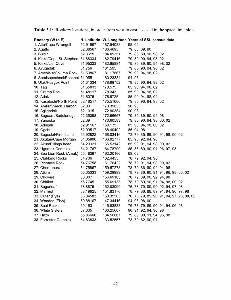
Table 3.1: Rookery locations, in order from west to east, as used in the space time plots.

Rookery (W to E) N. Latitude W. Longitude Years of SSL census data

1. Attu/Cape Wrangell 52.91667 187.54083 98, 02

2. Agattu 52.38567 186.4695 79, 88, 89, 90

3. Buldir 52.3615 184.09351 79, 88, 89, 90, 98, 02

4. Kiska/Cape St. Stephen 51.88334 182.79416 79, 89, 90, 94, 98, 02

5. Kiska/Lief Cove 51.95333 182.65884 79, 85, 89, 90, 94, 98, 02

6. Ayugadak 51.756 181.595 79, 85, 90, 94, 98, 02

7. Amchitka/Column Rock 51.53867 181.17867 79, 90, 94, 98, 02

8. Semisopochnoi/Pochnoi 51.955 180.23334 94, 98

9. Ulak/Hasgox Point 51.31334 178.98752 79, 85, 90, 94, 98, 02

10. Tag 51.55833 178.575 85, 90, 94, 98, 02

11. Gramp Rock 51.48117 178.343 85, 90, 94, 98, 02

12. Adak 51.6075 176.9725 85, 90, 94, 98, 02

13. Kasatochi/North Point 52.18517 175.51666 79, 85, 90, 94, 98, 02

14. Amlia/Sviech. Harbor 52.03 173.39833 90, 98

15. Agligadak 52.1015 172.90384 90, 98

16. Seguam/Saddleridge 52.35058 172.56667 79, 85, 89, 90, 94, 98

17. Yunaska 52.69 170.60583 79, 85, 90, 94, 98, 00, 02

18. Adugak 52.91167 169.175 85, 90, 94, 98, 00, 02

19. Ogchul 52.99517 168.40402 85, 94, 98

20. Bogoslof/Fire Island 53.92822 168.03416 73, 79, 85, 89, 90, 91, 98, 00, 02

21. Akutan/Cape Morgan 54.05906 166.02777 85, 90, 92, 94, 98

22. Akun/Billings head 54.29321 165.53142 85, 90, 91, 94, 98, 00, 02

23. Ugamak Complex 54.21767 164.78799 85, 86, 89, 90, 91, 96, 97, 98

24. Sea Lion Rock (Amak) 55.46367 163.20166 98, 02

25. Clubbing Rocks 54.706 162.4455 78, 79, 92, 94, 98

26. Pinnacle Rock 54.76758 161.76422 78, 79, 91, 94, 98, 00, 02

27. Chernabura 54.75867 159.57278 78, 79, 86, 90, 92, 94, 98

28. Atkins 55.05333 159.28999 78, 79, 86, 90, 91, 94, 96, 98, 00, 02

29. Chowiet 56.007 156.69183 78, 79, 89, 90, 92, 94, 98

30. Chirikof 55.7745 155.69133 78, 79, 89, 90, 91, 94, 98, 00, 02

31. Sugarloaf 58.8875 152.03999 76, 78, 79, 89, 90, 92, 94, 97, 98

32. Marmot 58.19625 151.83176 78, 79, 86, 88, 89, 91, 94, 96, 97, 98

33. Outer (Pye) 58.84583 150.39583 76, 78, 79, 89, 90, 91, 94, 97, 98, 00, 02

34. Wooded (Fish) 59.88167 147.34416 94, 96, 98, 00

35. Seal Rocks 60.163 146.83833 76, 78, 79, 89, 90, 91, 94, 96, 98

36. White Sisters 57.635 136.25667 90, 91, 92, 94, 96, 98

37. Hazy 55.86666 134.56667 79, 89, 90, 91, 94, 96, 98

38. Forrester Complex 54.83833 133.52667 73, 79, 82, 90, 91

43

4. Treating Observation Error

Pup counts should be fairly accurate, because pups are almost always on land during the

summer surveys. Thus, following Pascual and Adkison (1994), we use a sighting

probability of 1 for pups. In contrast, the number of non-pups counted in any rookery

census is nearly always smaller than the true number of individuals associated with the

site, because an unknown fraction of the animals were at sea at the time of counting. We

now show how to account for this observation error.

We estimate the distribution of observation error (the probability distribution for the

observed count given the “true” number of individuals present) using multiple censuses

conducted within the same season at the same site (available for three rookeries; see

below).

We only consider females in the model (Sections 5,6). Since about 75% of the non-pup

sea lions on rookeries are females, and about 50% of the pups are females (NRC 2003),

we multiply all non-pup counts by 0.75 and pup counts by 0.5 before using them.

Our likelihood-based approach requires us to calculate the probability of observing Nobs

non-pups given that Ntrue are actually present. We use a beta-binomial distribution

(Martz and Waller 1982, Evans et al 2000) to describe the number of individuals sighted

in a non-pup survey. In this approach, the probability of sighting an individual, Pobs,

varies from census to census according to a beta distribution defined by the parameters α

and β (Evans et al. 2000), so that the average value of the probability of sighting an

44

individual is α/(α+β). The values of these two parameters are unknown but assumed

constant across time and space. The variance of Pobs between censuses is given by

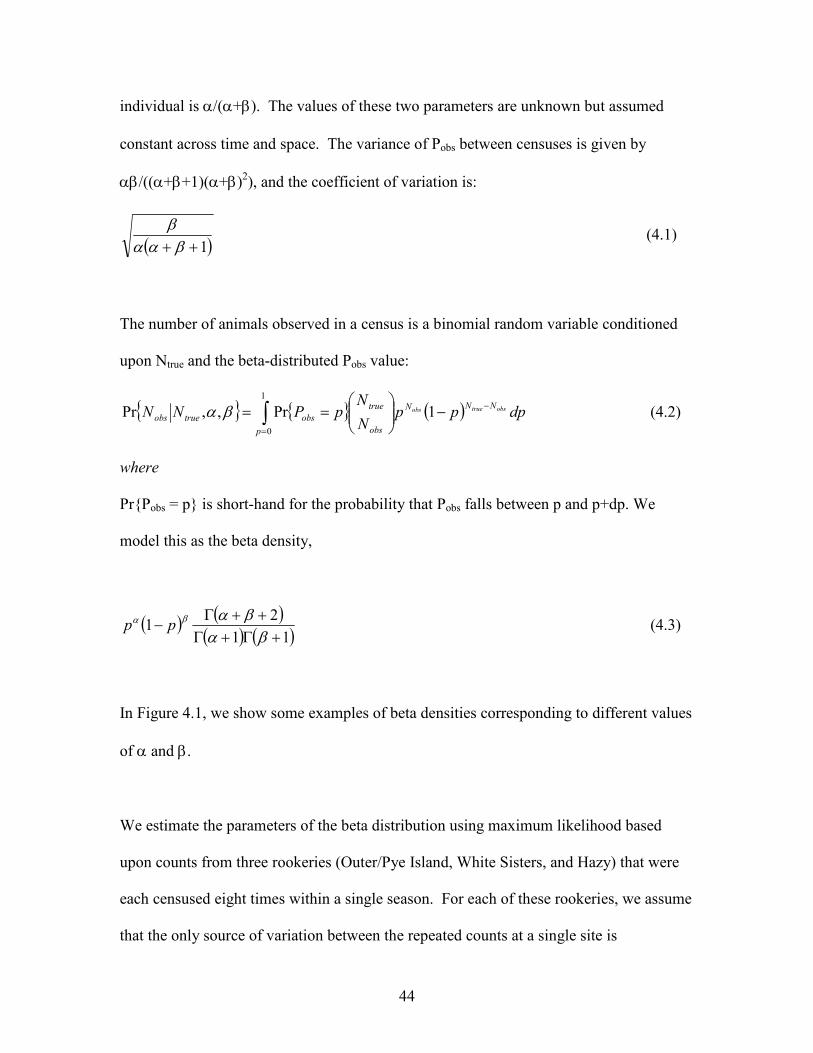
αβ/((α+β+1)(α+β)2), and the coefficient of variation is:

( )1++ βααβ

(4.1)

The number of animals observed in a census is a binomial random variable conditioned

upon Ntrue and the beta-distributed Pobs value:

{ } { } ( )∫=

−−

==

1

0

1Pr,,Prp

NNN

obs

true

obstrueobs dpppN

NpPNN obstrueobsβα (4.2)

where

Pr{Pobs = p} is short-hand for the probability that Pobs falls between p and p+dp. We

model this as the beta density,

( ) ( )( ) ( )11

21

+Γ+Γ++Γ

−βα

βαβα pp (4.3)

In Figure 4.1, we show some examples of beta densities corresponding to different values

of α and β.

We estimate the parameters of the beta distribution using maximum likelihood based

upon counts from three rookeries (Outer/Pye Island, White Sisters, and Hazy) that were

each censused eight times within a single season. For each of these rookeries, we assume

that the only source of variation between the repeated counts at a single site is

45

observation error. Since the true non-pup population numbers that produced the counts

are unknown, we need to integrate across a range of possible Ntrue values at each rookery

in order to calculate the likelihood for each set of α and β values. We do not know the

prior probability distribution for Ntrue, but our choice of error structure implies that the

expected ratio of Ntrue to Nobs at any rookery, given particular values of alpha and beta, is

the inverse of the mean of the beta distribution. Thus, the expected distribution of true

non-pup numbers among rookeries in a single year has the same shape as the distribution

of observed counts, and the distribution of Ntrue can be estimated (given α and β) by

horizontally expanding the Nobs distribution by a factor of (α+β)/α.

We construct prior probability distributions for Ntrue corresponding to each combination

of α and β values by fitting a log-normal distribution to the Nobs values from all rookery

counts recorded in a single year (1998: Fig. 4.2) and scaling it up by a factor of (α+β)/α.

We chose the data from 1998 for this purpose because more rookeries were censused in

that year than in any other. The Ntrue prior distribution is factored into the likelihood

calculations for α and β according to Bayes’ theorem (Hilborn and Mangel 1997).

The likelihood is calculated as follows:

Pr{Ntrue = n} is the prior probability distribution for Ntrue (see Fig. 4.1)

Pr{Pobs = p|α,β} is shorthand for the Beta density, as in Eqn 4.3

datai,k is the kth count recorded at the i

th rookery

and

46

Pr{datai,k|Ntrue = n,Pobs = p} = ( ) kiki datandata

ki

ppdata

n,, 1

,

−−

(4.4)

We then have

( ) { } { } { }∏∑ ∏ ∫=

∞

= = =

=====

3

1 0

8

1

,

1

0

,Pr,PrPr,i n k

obstrueki

p

obstrue dppPnNdatapPnNdataLikelihood βαβα (4.5)

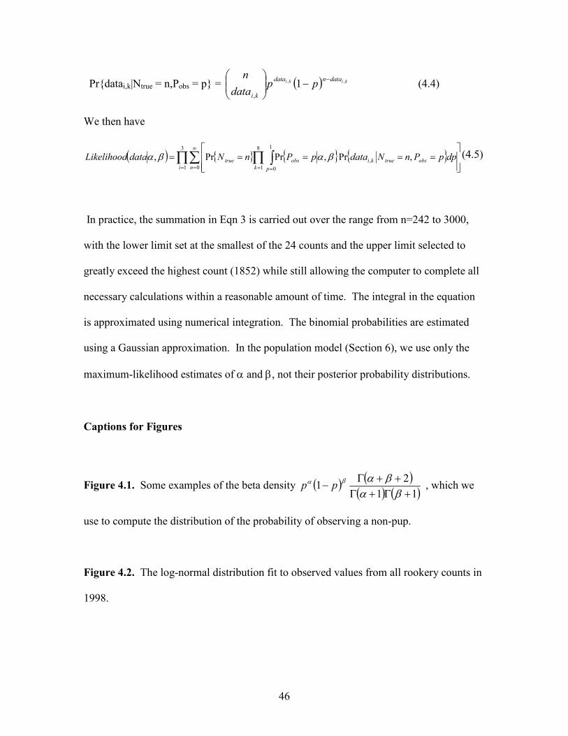
In practice, the summation in Eqn 3 is carried out over the range from n=242 to 3000,

with the lower limit set at the smallest of the 24 counts and the upper limit selected to

greatly exceed the highest count (1852) while still allowing the computer to complete all

necessary calculations within a reasonable amount of time. The integral in the equation

is approximated using numerical integration. The binomial probabilities are estimated

using a Gaussian approximation. In the population model (Section 6), we use only the

maximum-likelihood estimates of α and β, not their posterior probability distributions.

Captions for Figures

Figure 4.1. Some examples of the beta density ( ) ( )( ) ( )11

21

+Γ+Γ++Γ

−βα

βαβα pp , which we

use to compute the distribution of the probability of observing a non-pup.

Figure 4.2. The log-normal distribution fit to observed values from all rookery counts in

1998.

47

Table 4.1. Repeat counts from rookeries used for fitting the beta-binomial model of

observation error.

Rookery (Year)

Outer/Pye (1992)

White Sisters (1991)

Hazy (1991)

242 1040 1582 481 1153 1521 319 857 1562 477 905 1852 370 1011 1413 371 1041 1382 369 932 1375 391 860 1278 Mean 377.5 974.875 1495.625 SD 78.14638 103.826 177.7486 CV 0.20701 0.106502 0.118846

48

5. Vital Rates and Local Conditions

Our investigatory approach is based upon the assumption that sea lion vital rates vary

from rookery to rookery and year to year according to the local conditions around each

rookery in each year. Each of the competing hypotheses that have been raised to explain

the sea lions’ decline can be interpreted as a generalized linear model (Stefansson 1996)

relating mortality or fecundity rates to local conditions.

Population Model: Two Age Classes, Three Vital Rates

We assume that the population dynamics can be satisfactorily described in terms of 2 age

classes: pups and non-pups. We follow York (1994) in considering only females and

assume a 50-50 sex ratio (NRC 2003). Thus, the underlying variables are:

J(i,t) = Number of female pups at rookery i in year t.

Ntrue(i,t) = Number of female non-pups at rookery i in year t. (5.1)

We assume that the number of pups observed equals J(i,t) but that the number of non-

pups observed, Nobs(i,t), is less than or equal to the actual number of non-pups, Ntrue(i,t),

and use the model developed in Section 4 to relate the two.

Because the breeding season is relatively compressed, we assume discrete time dynamics

and no density dependence. In that case, there are three fundamental parameters at

rookery i in year t:

49

ρi,t= Probability of pup survival (recruitment to the non-pup population) from

year t to year t+1

σi,t = Probability of non-pup survival from year t to year t+1 (5.2)

φi,t = Per capita probability for non-pups of successful reproduction in year t.

We set fixed background values for these parameters (denoted by ρ0, σ0, and φ0) that are

modified by local conditions according to parameterized functions reflecting each

hypothesis. We estimate the background values from life tables based on data collected

on the Marmot Island rookery (Calkins and Pitcher 1982) and used by Pascual and

Adkison (1994) and York (1994), with corrections in Holmes and York (2003). The

annual growth rate of a population using the original life table is slightly more than 1%.

Since our model lumps together all age classes above 1 year, we calculate σ0 and φ0 by

integrating the survival and fecundity probabilities across all non-pup classes in the stable

age distribution produced by the life table:

ρ0 = 0.776

σ0 = 0.858

φ0 = 0.197

(5.3)

This fecundity estimate accounts for only about 50% of the pups being female (York

1994, NRC 2003) and for about 45% of the non-pup population being juvenile (Holmes

and York 2003). Our estimate is a little lower than the value used by York (1994), 0.315.

50

However, she only included the sexually mature age classes (3+) in her average, whereas

our simpler model lumps together all non-pup age classes (1+), including non-

reproductive juveniles.

Vital Rates as Functions of Local Conditions

Each hypothesis corresponds to a generalized linear model that produces a scaling factor

between 0 and 1 to modify the fecundity, recruitment, or survival rate at any rookery in

any year according to the corresponding local conditions. The relevant local conditions

may include prey abundance, fishing activity, predator abundance, or other factors,

depending on the hypothesis being tested.

We let ωn denote the symbol for the value of the vital rate modifier produced by the

function corresponding to hypothesis n. Each function contains a parameter, cn, that is

unknown, but which we assume is constant across all rookeries and years and which we

intend to estimate from the data. The local value of each vital rate (ρi,t, σi,t, or φi,t) is

calculated by multiplying the maximum potential rate (ρ0, σ0, or φ0) by all the relevant

scaling factors. We consider ten unknown parameters, one per hypothesis. In each case,

a parameter value of zero indicates that the corresponding hypothesis has no effect. The

ten hypotheses and their functional forms are described in detail below, and summarized

in Table 5.1.

51

H1-H3: Acute Nutritional Stress (Food Limitation) hypotheses

Low abundance of groundfish and other prey causes local fecundity (Hypothesis 1), pup

recruitment (Hypothesis 2), or non-pup survival probability (Hypothesis 3) to be

diminished. Specifically, we assume that the probability with which an animal avoids

starvation (ω2, ω3) or successfully produces a pup (ω1) follows a Type III functional

response (Holling 1959) with respect to the average total prey biomass, λtotal(i,t),

recovered per unit volume of standardized trawling effort within the foraging area around

rookery i during year t (Figure 5.1a):

ωn(i, t) =λtotal

2 (i,t)

cn2 + λtotal

2(i, t) (5.4)

where the subscript n indicates that hypothesis n is being considered, and

c1, c2, and c3 are the (unknown) parameters corresponding to each hypothesis. We refer

to these parameters as the half-saturation constant, since when λtotal(i,t)= cn ,

ωn(i, t) = 0.5.

Our choice of a sigmoid function (a Holling Type III functional response, Turchin 2003)

implies that sea lions are unlikely to find enough to eat when prey are scarce, and

unlikely not to find enough to eat when prey are abundant. The negative effect is

increasingly severe at lower food abundance levels. One could argue whether the Type II

or Type III functional response is more appropriate. This is an empirical, rather than

theoretical, question and a variety of papers in Boyd and Wanless (in prep – ZSL

52

Symposium 22/23 April 2004 “Management of Marine Ecosystems: Monitoring Change

in Upper Trophic Levels”) support the choice of a Type III functional response.

H4-H6: Chronic Nutritional Stress (Junk-food) hypotheses

As described in Section 1, there is general agreement that an abundance of walleye

pollock is not ‘good’ for sea lions, although the mechanism is still not fully understood.

Consequently, we assume that a high proportion of walleye pollock in the environment

causes local fecundity (Hypothesis 4), pup recruitment (Hypothesis 5), or non-pup

survival probability (Hypothesis 6) to be diminished.

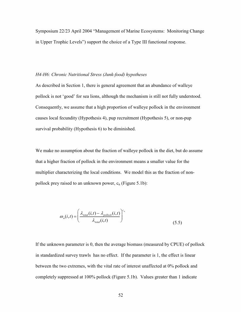
We make no assumption about the fraction of walleye pollock in the diet, but do assume

that a higher fraction of pollock in the environment means a smaller value for the

multiplier characterizing the local conditions. We model this as the fraction of non-

pollock prey raised to an unknown power, cn (Figure 5.1b):

ωn(i, t) =λtotal(i,t) − λpollock (i,t)

λtotal(i,t)

c n

(5.5)

If the unknown parameter is 0, then the average biomass (measured by CPUE) of pollock

in standardized survey trawls has no effect. If the parameter is 1, the effect is linear

between the two extremes, with the vital rate of interest unaffected at 0% pollock and

completely suppressed at 100% pollock (Figure 5.1b). Values greater than 1 indicate

53

strong suppression of the vital rate whenever pollock represents a significant fraction of

the total biomass (assessed via CPUE) in the environment:

H7, H8: Anthropogenic Activity (Fishery-related mortality) hypotheses

As described in Section 1, fisheries may have indirect effects on survival or fecundity by

removing prey or direct effects through entanglement in gear or shooting. For these

hypotheses, we assume that survival probability of pups (Hypothesis 7) or non-pups

(Hypothesis 8) is diminished in areas where there is more commercial fishery activity.

Specifically, the probability with which a pup or non-pup avoids having a fatal encounter

with a fishing boat is the Poisson probability of zero fatal encounters in a single year,

where the rate of fatal encounters is proportional to the total duration (minutes) of

commercial haul activity reported near the rookery, µ(i,t). The unknown proportionality

constant (= mortality rate per encounter) is cn (Figure 5.1c):

( ) ( )tic

nneti

,,

µω −= (5.6)

Equation 5.6 can be derived from first principles of random search (Hilborn and Mangel

1997), but has also been found (Washburn 1981) to effectively characterize encounters

that are non-random.

54

H9, H10: Predation mortality hypotheses

The notion that the sequential collapse of populations of harbor seals, Steller sea lions,

and sea otters (sensu Springer et al 2003) is due to killer whale predation relies on the

assumption of expanding diet breadth for orcas. We approach this from the viewpoint of

rate-maximizing diet choice theory (Stephens and Krebs 1986), which we now briefly

review.

The classic diet choice model begins with the assumption that Darwinian fitness (the

long-term number of descendants, often approximated by the expected lifetime

reproductive success) is maximized when the rate at which energy is obtained is

maximized. As we note below, killer whales often hunt in groups. Group hunting is a

complicating factor, but it does not necessarily affect the validity of the assumption of

rate maximization (Mangel 1992). The suite of prey species is characterized by 1) the net

energy Ei (units, kcal) obtained by chasing, killing and consuming a single individual of

prey type i; 2) the time Hi (units, hours) needed to “handle” (chase, kill and consume) a

single individual of prey type i; and 3) the encounter rate ri (units, 1/hours) with prey type

i. One then assumes that the major activities of the predator consist of searching for prey

and handling prey. Thus, any long period of time T is divided into a total time spent

searching S and a total time spent handling H. These assumptions are sufficient to

compute the long-term rate of energy gain for any diet selection rule that the predator

uses. One then chooses the diet selection composition that maximizes the rate of energy

return.

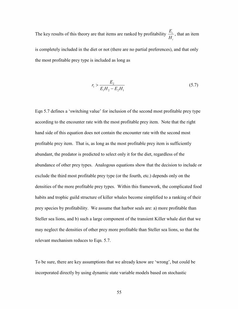
55

The key results of this theory are that items are ranked by profitability i

i

H

E, that an item

is completely included in the diet or not (there are no partial preferences), and that only

the most profitable prey type is included as long as

1221

21

HEHE

Er

−> (5.7)

Eqn 5.7 defines a ‘switching value’ for inclusion of the second most profitable prey type

according to the encounter rate with the most profitable prey item. Note that the right

hand side of this equation does not contain the encounter rate with the second most

profitable prey item. That is, as long as the most profitable prey item is sufficiently

abundant, the predator is predicted to select only it for the diet, regardless of the

abundance of other prey types. Analogous equations show that the decision to include or

exclude the third most profitable prey type (or the fourth, etc.) depends only on the

densities of the more profitable prey types. Within this framework, the complicated food

habits and trophic guild structure of killer whales become simplified to a ranking of their

prey species by profitability. We assume that harbor seals are: a) more profitable than

Steller sea lions, and b) such a large component of the transient Killer whale diet that we

may neglect the densities of other prey more profitable than Steller sea lions, so that the

relevant mechanism reduces to Eqn. 5.7.

To be sure, there are key assumptions that we already know are ‘wrong’, but could be

incorporated directly by using dynamic state variable models based on stochastic

56

dynamic programming (Mangel and Clark 1988, Clark and Mangel 2000). We have

ignored physiological state (both energetic reserves and gut content) of the killer whales,

and these can often affect the predictions of diet breadth (Mangel and Clark 1988,

Mangel 1992, Clark and Mangel 2000) in subtle ways. We also know that killer whales

hunt in groups and that there is individual variation in group formation and social

interactions (Baird 2000). The classic diet choice model can be extended to include each

of these, but such extensions are beyond the scope of this work (Mangel 1992), and rate

maximizing has proven itself to be a reasonable, if not totally realistic, starting point for

many questions in behavioral ecology (Stephens and Krebs 1986).

Thus, we assume that pup survival (Hypothesis 9) and/or non-pup survival (Hypothesis

10) decrease(s) when harbor seal numbers at rookery i in year t, h(i,t), fall below a critical

level, hcrit. Below this harbor seal density, the encounter rate between Killer whales and

harbor seals is so low that the average profitability of a sea lion exceeds the average

intake rate of a Killer whale searching only for seals, and a rate-maximizing whale is

predicted to begin to hunt sea lions as well as seals. In particular, if Killer whales expand

their diets when harbor seal numbers are too low, then ωn(i,t)=1 if h(i,t)>hcrit and

ωn(i,t)=1-cn otherwise, with hcrit and cn to be determined.

Thus, if Killer whale predation is a significant source of mortality for Steller sea lions,

the average density of harbor seals around sea lion rookeries with rising populations

should be higher than that around rookeries with falling populations. The critical harbor

seal density is predicted to lie in between these two distributions. We therefore estimate

57

hcrit as the midpoint between the harbor seal density averages for sea lion rookeries with

rising and falling populations (Section 7).

Putting it all together

The ‘full’ model, which accounts for all 10 hypotheses, is one in which the life history

parameters take the form:

φ(i,t) = φ0ω1( i,t)ω4 (i, t)

ρ(i, t) = ρ0ω2 (i,t)ω5 (i,t)ω7(i,t)ω9 (i, t)

σ(i,t) = σ 0ω3 (i, t)ω 6(i, t)ω8(i,t)ω10(i, t) (5.8)

As mentioned previously, we assume that the parameters c1-c10 in the ten hypothesized

functions are constant across space and time and we estimate them from the relevant data.

Note that if cn=0, then ωn(i,t)=1 and we conclude that Hypothesis n has no effect on the

relevant life history parameter; this gives a prelude of what is to come in the statistical

analysis: If, as a result of our confronting the models with data we conclude that the best

estimate for cn=0, then the associated particular mechanism is unlikely to play a

significant role in the dynamics of the Steller sea lions. If, on the other hand, we

conclude that cn>>0, then the associated mechanism is likely to play a critical role in the

dynamics. In Section 6, we make these ideas more precise in terms of the Maximum

Likelihood Estimate (MLE) of the parameter and the 95% confidence interval for that

parameter.

58

We can also investigate any particular combination of sub-models by setting the

associated cn=0, or (equivalently), ωn(i,t)=1.

Caption for Figure

Figure 5.1. The functional forms that we use to calculate vital rates from the local

conditions matrices according to the acute nutritional stress hypotheses (panel a), the

chronic nutritional stress hypotheses (panel b) and the anthropogenic mortality

hypotheses (panel c).

Table 5.1. The ten hypotheses and their respective parameters.

Hypothesis Parameter

H1: Prey CPUE → fecundity c1, prey density at which fecundity is half of potential rate

H2: Prey CPUE → pup recruitment c2, prey density at which recruitment is half of potential rate

H3: Prey CPUE → non-pup survival c3, prey density at which non-pup survival is half of potential rate

H4: Pollock fraction → fecundity c4, exponent of non-pollock prey fraction in fecundity multiplier

H5: Pollock fraction → pup recruitment c5, exponent of non-pollock prey fraction in recruitment multiplier

H6: Pollock fraction → non-pup survival c6, exponent of non-pollock prey fraction in non-pup survival multiplier

H7: Fishing activity → pup recruitment c7, pup mortality rate per minute of haul time

H8: Fishing activity → non-pup survival c8, non-pup mortality rate per minute of haul time

H9: HS density → SSL pup recruitment c9, fraction of potential recruitment lost when harbor seals < hs_crit

H10: HS density → SSL non-pup survival c10, fraction of potential non-pup survival lost when HS < hs_crit

H9, H10 hcrit, harbor seal density below which sea lions become prey

59

6. A Model that Connects the Hypotheses and the Data

In previous sections, we have defined functional forms for our ten hypotheses, outlined

our population model, and shown how to account for observation error. We must now

connect the observed census data and the unknown local vital rate function parameters

with each other through the stochastic population dynamics of the stock.

The basic approach is as follows: Starting with the beta-binomial observation error

distribution and a two-life-stage stochastic population model employing the local vital

rates, we calculate the probability of observing the sequence of reported pup and non-

pup counts at a particular rookery, given (1) relevant local conditions and (2) a particular

set of parameter values in the hypothesized equations. We find this probability using

backwards iteration and by “thinking along sample paths,” which essentially amounts to

averaging across many possible true population trajectories that each could have

produced the observed sequence of census data.

Analogous probabilities are calculated for all rookeries and censuses and multiplied

together to estimate the likelihood of the data given the hypotheses and each possible set

of parameter values. The likelihood profile for each parameter is calculated while

holding all the other parameters at their respective MLEs (Maximum Likelihood

Estimates). Using Bayes’ theorem (Hilborn and Mangel 1997) and a uniform prior

probability distribution for each parameter, we convert the likelihoods into posterior

probability distributions and estimate confidence intervals from them, allowing us to

60

quantify the relative strengths of the corresponding hypotheses. Strictly speaking, each

parameter’s posterior distribution calculated in this way is contingent upon an assumption

that the MLE values of the other nine parameters are approximately correct. However,

our data set is sufficiently large that we can neglect this issue (Kalbfleisch and Sprott

1970).

In contrast to all previous modeling approaches, we do not require a complete data set,

and we make use of variation both between rookeries and across time. The details of our

approach are outlined below.

The Basic Population Dynamics

As already noted, we assume that the population dynamics can be described by two age

classes: pups (J(i,t), age <1 year) and non-pups (N(i,t), age 1+). We follow York (1994)

in considering only females. The three relevant vital rates are:

ρi,t= Probability of pup survival (recruitment to non-pup class) from year t to t+1

σi,t = Probability of non-pup survival from year t to year t+1

φi,t = Probability of successful pup production by a non-pup in year t. (6.1)

In the absence of stochasticity, the population dynamics would be given by:

N(i,t+1) = ρi,tJ(i,t) + σi,tN(i,t) (6.2a)

J(i,t+1) = φi,tN(i,t+1) (6.2b)

61

If all parameters were constant, then the dynamics in Eqn 6.2 would generate population

growth or decline according to the dynamics

N(i,t+1) = [ρ φ + σ]N(i,t) (6.3)

For the base case parameters given in Eqn 5.3, this corresponds to a growth rate of just

over 1% per year. However, the parameters are not constant (they vary according to local

conditions), and the transitions in Equation 6.3 are stochastic, not deterministic. Thus,

we must deal with process uncertainty.

Accounting for Process Uncertainty

Each of the life history parameters is bounded by 0 and 1, so that we can think of them as

binomial transition probabilities of non-pup survival and reproduction and pup survival.

The probability distributions for true numbers of non-pups and pups at time t, given the

numbers at t-1, are therefore computed from the associated binomial distributions. In the

equation for the non-pup distribution, we sum across all possible numbers of pups

(j=0,1,2...N(t-1)) at time t-1, multiplying the probability associated with each j value by a

convolution of binomials that accounts for all the possible permutations of surviving non-

pups (s = 0,1,2...N(t-1)) and recruiting pups (r = N(t)-s) that could have produced N(t)

non-pups at time t, given N(t-1) non-pups and j pups at time t-1. If we let

( ) ( ){ }1Pr −tNtN denote the probability that the non-pup population in year t is N(t) given

that the non-pup population in year t-1 was N(t-1), then

62

{ })1()(Pr −tNtN

( ) ( ) ( ) ( )( )

∑ ∑−

=

−

=

−−−−−−−−

−

−

−−

−−

−=

)1(

0

)(),1(min

0

)()1()()1()1(1

)(

)1(1

)1(1

)1(tN

j

tNtN

s

stNtJstNstNsjtNj

stN

tJ

s

tN

j

tNρρσσφφ (6.4)

Alternatively, one might consider that at time t-1 there were N(t-1) non-pups and N(t-1)

“potential pups,” reflecting the fact that each non-pup can produce a pup. In this

interpretation, we multiply the fecundity and recruitment probabilities together rather

than dealing with them separately. The resulting equation

{ } ( ) ( ) ( ) ( )( )

∑−

=

−−−−−−

−

−

−−

−=−

)(),1(min

0

)()1()()1(1

)(

)1(1

)1()1()(Pr

tNtN

s

stNtNstNstNs

stN

tN

s

tNtNtN φρφρσσ (6.5)

is therefore equivalent to Equation 6.4.

If the number of pups at time t-1 is known, then we do not need to sum across possible

pup numbers, and Eqn 6.5 becomes:

{ } ( ) ( ) ( )( )

∑−

=

−−−−−−

−

−

−−

−=−−=

)(),1(min

0

)()1()()1(1

)(

)1(1

)1()1(),1()(Pr

tNtN

s

stNtJstNstNs

stN

tJ

s

tNtJtNntN ρρσσ (6.6)

Finally, the probability distribution for pups given the number of non-pups at time t is a

single binomial:

{ } ( ) )()()( 1)(

)()()(Pr

tJtNtJ

tJ

tNtNtJ

−−

= φφ (6.7)

63

What remains is to connect the probabilistic dynamics given by these equations to the

observed data. We do this next.

Thinking Along Sample Paths

We want to find the values of the parameters in the local condition matrix that give the

highest probability of observing all the reported SSL counts, using all of the data at hand.

To do this, we take advantage of the rules of probability. In particular, if Pr{A|B}

indicates the probability of the event A, given the event B, then (Mangel and Clark 1988)

Pr{A | B} = Pr{A | C}Pr{C | B}

C

∑ (6.8)

where the sum is taken over all the events (or states) C that can occur between B and A.

In physics, this approach is known as path integration (Shulman 1981) and was first made

very useful by Richard Feynman in his formulation of quantum mechanics (Feynman

1948). For that reason, we call it the method of ‘thinking along sample paths’.

We illustrate the ideas in Figure 6.1. We begin with a series of censuses, not necessarily

in consecutive years (Figure 6.1a). Associated with each census (represented by the solid

dot in Figure 6.1a) is a probability distribution for the true number of non-pups, which is

larger than the observed number (as discussed in the previous section). We now

recognize (Figure 6.1b) that there is a very large number of trajectories of population size

that might connect the census values. In actual fact, the situation is a bit more

complicated than Figure 6.1b, because we must consider counts of both pups and non-

pups (Figure 6.1c, in which we show one trajectory ).

64

Looking Backward

The likelihood associated with a particular set of parameter values is estimated as the

product of the likelihoods for all rookeries. Likelihood for an individual rookery is

calculated using backwards iteration, which is an efficient way to consider many different

possible “sample paths” simultaneously. First, we consider a range of possible values for

Ntrue(T), the true number of non-pups at the time of the latest available census, and

calculate, for the given combination of parameters, the probability of observing the

reported non-pup and pup counts (Nobs(T) and J(T)), using Eqns 4.2 and 4.3 for non-pups

and assuming no observation error for pups. Second, we move to the previous year (T-1)

and use Equations 6.5 and 6.7 to calculate, for a range of possible Ntrue(T-1), the

probability of making the transition to each Ntrue(T) value considered in the first step.

This involves integrating over all the possible combinations of recruiting pups and

surviving non-pups that could produce each Ntrue(T) value, as in Equation 6.4 or 6.5. For

each Ntrue(T-1), the likelihood of observing J(T) and Nobs(T) is the sum of the

probabilities calculated in the first step, weighted by the integrated binomial probabilities

corresponding to each possible transition from Ntrue(T-1) to Ntrue(T). Formally expressed,

we have:

( ) ( ) ( ){ }1,Pr −TNTNTJ trueobs

( ) ( ){ } ( ) ( ){ } ( ) ( ){ }[ ]( )∑∞

=

=−===TNn

truetruetruetrueobs

obs

nTNTJTNnTNnTNTN Pr1PrPr (6.9)

where

65

( ) ( ){ }nTNTN trueobs =Pr is calculated using numerical integrations of Eqns 4.2 and 4.3,

( ) ( ){ }1Pr −= TNnTN truetrue is calculated using a Gaussian approximation of Eqn 6.5, and

( ) ( ){ }nTNTJ true =Pr is calculated using Eqn 6.7.

In practice, the summation in equation 6.9 is carried out in steps of 20 over the range

from Nobs(T) to 11417, with this upper limit set to the highest estimated female non-pup

count (6380) multiplied by a factor of (α+β)/α. We chose a step size of 20 for Ntrue in

order to minimize computer run-time without noticeably altering the shape of the output

likelihood curves.

If T-1 was a census year, we also multiply by the probability of observing Nobs(T-1) and

J(T-1), given each possible true non-pup count at T-1. That is,

( ) ( ) ( ) ( ) ( ){ }1,,1,1Pr −−− TNTNTJTNTJ trueobsobs

= [ ( ) ( ){ } ( ) ( ){ }11Pr11Pr −−−− TNTJTNTN truetrueobs

( ) ( ){ } ( ) ( ) ( ){ } ( ) ( ){ }[ ]( )∑∞

=

=−−==⋅TNn

truetruetruetrueobs

obs

nTNTJTJTNnTNnTNTN Pr1,1PrPr ] (6.10)

where

( ) ( ){ }11Pr −− TNTN trueobs is calculated using numerical integrations of Eqns 4.2 and 4.3,

( ) ( ){ }11Pr −− TNTJ true is calculated using Equation 6.7,

( ) ( ){ }nTNTN trueobs =Pr and ( ) ( ){ }nTNTJ true =Pr are calculated as above, and

66

( ) ( ) ( ){ }1,1Pr −−= TJTNnTN truetrue is estimated using a Gaussian approximation of Eqn

6.6.

Analogous procedures are used to calculate the probabilities of observing all reported

counts from T-2 onwards, given a range of possible values for Ntrue(T-2). Then the

process is repeated for T-3, T-4, etc. until we reach the earliest recorded census at tstart.

Model likelihood for a single rookery is calculated as the average of the likelihoods of all

possible trajectories starting at each possible combination of observed true pup and

unknown non-pup numbers, J(tstart) and Ntrue(tstart). The equal weight given to each

trajectory likelihood in this average reflects our use of a flat (uniform) prior probability

distribution for the unknown Ntrue(tstart). Overall model likelihood is calculated as the

product of the likelihoods from all rookeries.

The likelihood of a model with parameters {cn, n=1..10} given the census data is then:

{ } ( ){ } ( ) ( ) ( ){ }( )

∑ ∏

=

starttrue tiN

possibleall

censuses

allstarttrueobsstarttrue etcccctiNtiJtiNtiNdatacccL

,

_10211021 .,,,,...,,,,,,Pr,Pr,..., βα

(6.11)

We now view the data as fixed (which it is), so that L{c1,c2 ,...c10 | data} is a 10-

dimensional function of the unknown parameters. In many other settings, some

parameters are known a priori to be of interest and other parameters not; they are often

67

called nuisance parameters. There exists a considerable literature that explores how

likelihood methods can deal with nuisance parameters (e.g. Kalbfleisch and Sprott 1970;

Edwards 1992; Royall 1997; Sorensen and Gianola 2002). The situation that we consider

is somewhat different, because we are a priori interested in all of the 10 parameters, but

seek a practicable way to envision the output. Based on examination of the literature, we

have settled on the following procedure to estimate the values of the parameters and the

evidence that the data provide about the strength of the effect associated with each

parameter. Royall (1997) notes that there is no general solution to this problem and no

existing approach that is theoretically unassailable, but that “there are a variety of quite

satisfactory ad hoc methods for many important applications” (pg 152).

We searched the 10-dimensional parameter space for the values of the constants that

maximize the likelihood function. We denote these maximum likelihood estimates

(MLEs) by ci*

. Next, we constructed 10 one-dimensional functions by holding 9 of the

parameters at their maximum likelihood value and systematically varying the 10th across

the range of values where likelihood is appreciable. Thus, for example, for the parameter

associated with hypothesis H1, the function we consider is ( )datacccL ,,..., *

10

*

21 (for

purposes of presentation in figures, we use log-likelihoods). This is called the profile

likelihood for parameter c1; the definitions of the other 9 profile likelihoods are similar.

In the next section, we will show plots of the 10 profile likelihoods.

We will also introduce the profile likelihood interval, defined as the upper and lower

limits of the shortest segment under the likelihood curve that contains 95% or 99% of the

total area under the curve. These points are often approximated as the intersections

68

between the log-likelihood curve and a horizontal line drawn several units below the

maximum likelihood (Hudson 1971). However, because many of our curves are

asymmetrical and/or have their peak at or near zero, we calculate the confidence intervals

more precisely using numerical integration (with the range of values considered for each

parameter divided into 20 steps) and interpolation. To the extent that the profile

likelihood can be considered a true likelihood curve (see below), this interval can be

interpreted as a true posterior confidence interval given a uniform prior probability

distribution for each parameter.

Kalbfleisch and Sprott (1970) and Sorensen and Gianola (2002) note that problems arise

when the number of parameters to be estimated is large relative to the number of data

points, but that if the number of parameters is relatively small, then the profile likelihood

can be viewed as a true likelihood function. In our case, we have 10 parameters and 167

censuses (123 census intervals), so that the number of parameters is indeed small relative

to the amount of data.

We will say that the data provide strong evidence for a hypothesis if the MLE of the

parameter associated with that hypothesis is non-zero and the profile likelihood interval

does not include 0. The data provide weak evidence for a hypothesis if the MLE of the

parameter associated with that hypothesis is non-zero but the profile likelihood interval

includes 0. If the MLE is 0, the data provide no evidence for the hypothesis.

Furthermore, we will classify the hypotheses as having a strong effect, a weak effect, or

no effect, depending upon how the MLE value of the parameter affects the predicted

69

population dynamics of Steller sea lions. Specifically, for each possible formulation of

the model, we look at the difference between the deterministic annual population growth

rate calculated from Eqn 6.3 according to the model and that calculated from the same

equation using the background vital rates (about 1.1%).

Caption for Figure

Figure 6.1. The method of ‘thinking along sample paths’ allows use to connect censuses

in different years (panel a) with underlying population trajectories (panel b), even in the

more complicated case of both pups and non-pups (panel c). Further details are given in

the text.

70

7. Results and Interpretations

Observation Error

The maximum-likelihood estimates of α and β are approximately 19 and 15, respectively

(Figure 7.1). Our characterization of the distribution for observation error (Figure 7.2)

results in a mean probability of observing a non-pup of about 56%.

Critical Harbor Seal Density

Harbor seal densities around rookeries with rising or falling sea lion populations are

shown in Figure 7.3 for three different years: 1980, 1990, and 2000. Consistent with the

prey switching hypotheses (H9, H10), all three years show higher mean harbor seal

densities (> 5000) where the sea lion population is growing, and lower densities (< 4000)

where the sea lion population is falling. The difference is statistically significant in 1990

(p = 0.004). We chose an intermediate harbor seal density (4500) as the threshold

parameter below which killer whales and/or other predators switch to consuming Steller

sea lions.

Confronting the Hypotheses With Data

The log-profile likelihood plots for the parameters associated with each hypothesis are

shown in Figure 7.4. In Table 7.1, we provide the MLE values for these parameters

along with their 95% confidence intervals. The evidence can be summarized as follows:

71

Strong Evidence Weak Evidence No Evidence

Strong Effect H1: Total prey

availability affects

fecundity

H5: Pollock

fraction affects pup

recruitment

Moderate Effect H10: Harbor seal

density (predation)

affects non-pup

survival

Weak or No Effect H4: Pollock

fraction affects

fecundity

H2: Total prey

availability affects

pup recruitment

H3: Total prey

availability affects

non-pup survival

H6: Pollock

fraction affects non-

pup survival

H7: Fishery activity

affects pup

recruitment

H8: Fishery activity

affects non-pup

survival

H9: Harbor seal

density (predation)

affects pup

recruitment

We consider that H4 only has weak evidence because the 95% and 99% confidence

intervals both include 0.

In Table 7.2, we give the Akaike Information Criterion (AIC) and AIC Weight for

thirteen of the most likely model configurations. Two models, one including H1, H4, H5,

and H10 and the other including only H1, H5, and H10, have very similar AIC weights

and together comprise almost 99% of the total weight. The third most likely model,

72

including H1 and H5, brings the cumulative total to 99.5%.

Forward Comparisons

In Figure 7.5, we compare non-pup census data to the results of forward simulations

based on different model configurations for three rookeries in the western population and

one in the eastern population. In Figure 7.5a, the simulation uses the fixed background

vital rates measured at the Marmot Island rookery (Calkins and Pitcher 1982, York 1994,

Holmes and York 2003). In panels b, c, d, and e, the vital rates are modified according to

hypotheses H1, H4, H5, and H10 alone, using the MLE values of their respective

parameters. Panel f includes both of the significant effects acting simultaneously. The

solid line in each graph shows the annual median value from 10,000 Monte Carlo

simulations starting at a single non-pup count chosen to minimize the sum-of-squares

difference between the observed censuses and the mean of the simulated trajectories. The

dotted lines correspond to the 2.5 and 97.5 percentiles of the simulated observed counts.

If we compare Figures 7.5b, c, d, and e, we see that H5 has by far the strongest effect,

followed by H1, H10, and finally H4. A comparison of Figures 7.5d and f reveals that

H5 can nearly explain the entire decline by itself.

73

Captions for Figures

Figure 7.1. Likelihood contours for the parameters of the beta distribution used to

characterize the observation error.

Figure 7.2. The resulting distribution for the probability of sighting a non-pup has a

peak at about 60%, and essentially all of the probability is contained between 40% and

80%.

Figure 7.3. When we compare the harbor seal populations around rookeries where

Steller sea lion populations were increasing (clear) or declining (grey) we see a clear (and

sometimes statistically significant) division with more harbor seals around those

rookeries that are increasing. We choose a density of 4500 harbor seals within the 300

km foraging radius of a rookery as the threshold for inclusion of Steller sea lions in the

diet of killer whales.

Figure 7.4. Profile likelihoods for the parameters associated with each of the hypotheses.

The weight of the evidence supports only H1 (that fecundity is a function of total prey

availability), H4 (that fecundity is a function of pollock fraction), H5 (that pup

recruitment is a function of pollock fraction), and H10 (that non-pup survival is a

function of harbor seal density).

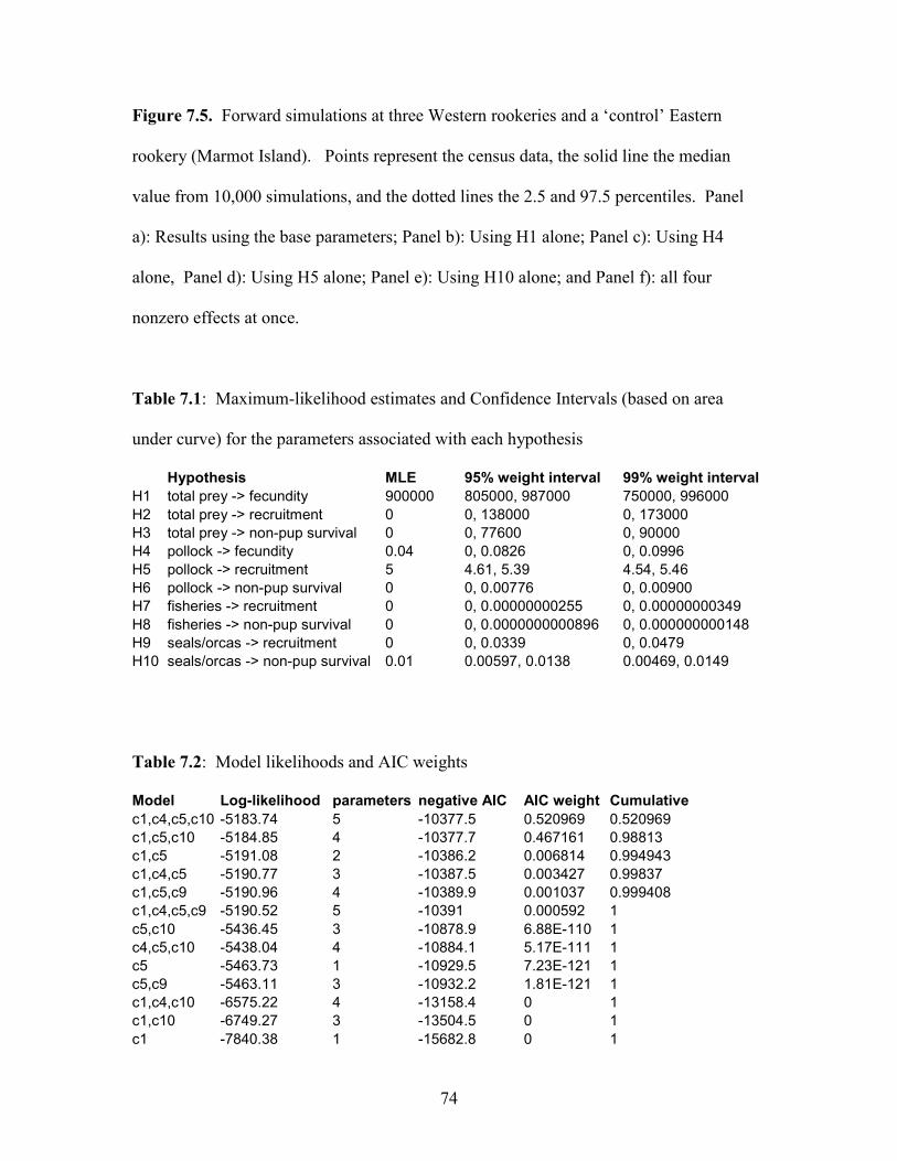
74

Figure 7.5. Forward simulations at three Western rookeries and a ‘control’ Eastern

rookery (Marmot Island). Points represent the census data, the solid line the median

value from 10,000 simulations, and the dotted lines the 2.5 and 97.5 percentiles. Panel

a): Results using the base parameters; Panel b): Using H1 alone; Panel c): Using H4

alone, Panel d): Using H5 alone; Panel e): Using H10 alone; and Panel f): all four

nonzero effects at once.

Table 7.1: Maximum-likelihood estimates and Confidence Intervals (based on area

under curve) for the parameters associated with each hypothesis

Hypothesis MLE 95% weight interval 99% weight interval

H1 total prey -> fecundity 900000 805000, 987000 750000, 996000

H2 total prey -> recruitment 0 0, 138000 0, 173000

H3 total prey -> non-pup survival 0 0, 77600 0, 90000

H4 pollock -> fecundity 0.04 0, 0.0826 0, 0.0996

H5 pollock -> recruitment 5 4.61, 5.39 4.54, 5.46

H6 pollock -> non-pup survival 0 0, 0.00776 0, 0.00900

H7 fisheries -> recruitment 0 0, 0.00000000255 0, 0.00000000349

H8 fisheries -> non-pup survival 0 0, 0.0000000000896 0, 0.000000000148

H9 seals/orcas -> recruitment 0 0, 0.0339 0, 0.0479

H10 seals/orcas -> non-pup survival 0.01 0.00597, 0.0138 0.00469, 0.0149

Table 7.2: Model likelihoods and AIC weights

Model Log-likelihood parameters negative AIC AIC weight Cumulative

c1,c4,c5,c10 -5183.74 5 -10377.5 0.520969 0.520969

c1,c5,c10 -5184.85 4 -10377.7 0.467161 0.98813

c1,c5 -5191.08 2 -10386.2 0.006814 0.994943

c1,c4,c5 -5190.77 3 -10387.5 0.003427 0.99837

c1,c5,c9 -5190.96 4 -10389.9 0.001037 0.999408

c1,c4,c5,c9 -5190.52 5 -10391 0.000592 1

c5,c10 -5436.45 3 -10878.9 6.88E-110 1

c4,c5,c10 -5438.04 4 -10884.1 5.17E-111 1

c5 -5463.73 1 -10929.5 7.23E-121 1

c5,c9 -5463.11 3 -10932.2 1.81E-121 1

c1,c4,c10 -6575.22 4 -13158.4 0 1

c1,c10 -6749.27 3 -13504.5 0 1

c1 -7840.38 1 -15682.8 0 1

75

8 Discussion

The strong message of ecology is that the world changes and that the reasons for change

are manifold. Thus, rather than trying to ‘prove’ one mechanism, we should recognize

that multiple mechanisms will almost always be at work, and we should ask how to

weigh the importance of different mechanisms. It is this approach that we’ve taken in

understanding the decline of the western population of Steller sea lions. Based on the

best set of data examined to date, we conclude that:

There is good evidence for two strong effects

H1: Total prey availability affects fecundity

H5: Pollock fraction in the environment affects pup recruitment.

and one moderate effect,

H10: Harbor seal density (predation) affects non-pup survival

marginal evidence for one weak effect,

H4: Pollock fraction in the environment affects fecundity

and no evidence at all for any of the other six effects considered:

H2: Total prey availability affects pup recruitment

H3: Total prey availability affects non-pup survival

H6: Pollock fraction in the environment affects non-pup survival

H7: Fishery activity affects pup recruitment

76

H8: Fishery activity affects non-pup survival

H9: Harbor seal density (predation) affects pup recruitment

Virtually all of the AIC weight (98.7%) is assigned to two models (one with H1, H4, H5,

and H10 and the other with H1, H5, and H10), suggesting that these three or four

hypotheses (or analogous ones that have the same apparent behavior) are sufficient to

explain the decline.

These results are not unexpected (indeed, each of the 10 hypotheses is plausible and has

been proposed at some point, with associated supporting data). What our work has done

is to guide the weight of the evidence, when all plausible hypotheses are competing,

towards those that win the competition.

However, the predicted population trajectories at Hazy (in the eastern stock) in Figure

7.5f are far too low. This suggests that the current model formulation has not yet

captured some important factor that differs between the western and eastern stocks. This

and a range of other possible follow-on projects are discussed in Appendix A.1.

Implications

Although we use the word mechanism, we recognize that a study such as this one cannot

demonstrate causality. But our work can suggest key empirical studies. To see this, let

us return to the deterministic version of the population model:

77

N(i,t+1) = ρ(i,t)J(i,t) + σ(i,t)N(i,t)

J(i,t+1) = φ(i,t)N(i,t+1) (8.1)

for which we now have life history parameters

φ(i,t) = φ0ω1( i,t)ω4 (i, t)

ρ(i, t) = ρ0ω5(i,t) (8.2)

σ(i,t) = σ 0ω10(i, t)

Eqn 8.1 can also be rewritten as

N(i,t+1) = [φ(i,t) ρ(i,t) + σ(i,t)]N(i,t) (8.3)

which gives us a simple way of measuring the decline or growth of the population.

Combining the various data described in Section 3 with these life history parameters

allows us to construct space-time plots for the decline rate, which we show in Figure 8.1.

Were we to speculate, it would seem that H1 is a relatively clear and simple mechanism:

that lower abundance of all prey types leads to lower fecundity through the direct effect

of reduced resource accumulation by adults and thus reduced storage for reproduction.

H10 also has a clear mechanism, but note that its MLE is about 0.01, so that the effect of

adaptive diet breadth by killer whales leads to only a 1% reduction in non-pup survival,

and then only in cases where harbor seal numbers are sufficiently low.

78

On the other hand, H4 and H5 are more complicated. A high pollock fraction can result

either from high pollock or from low non-pollock, and either of these could be the

underlying factor. Furthermore, the mechanism might be something completely different

for which pollock fraction is only a correlate. For example, juveniles may require some

easily caught subset of prey species because they are unable to dive deep enough or

swim fast enough to catch the prey that is better for them. (In the current data set the fish

biomass is not broken down by size class of fish. However, the really small fish and the

really big ones are probably not useful to sea lions. Thus, some additional thinking is

required about how to modify the survey data to address this question.)

Our results also suggest an adaptive management plan in which one designates the areas

around some of the rookeries as experimental zones in which to make fishery quotas

contingent upon the results of pre-fishing season survey trawls. We envision a series of

treatments:

• Rookeries around which fishing is not affected by the pre-season survey

information (control type 1).

• Rookeries around which no fishing occurs (control type 2)

• Rookeries around which fishing is reduced or prohibited if the total prey biomass

in the pre-season zone is below a critical threshold (determined by c1).

• Rookeries around which a directed pollock fishery occurs if the pre-season survey

suggests pollock fraction is above a critical threshold (determined by c5).

79

This combination of rookery types would allow sufficient variation in treatment, which is

crucial in adaptive management (MRAG Americas 2002). Sea lion vital rates would be

monitored in the same areas to see if the management plan is having a positive effect.

Before organizing any adaptive management, it would be possible to use our model to

simulate forward and suggest a time scale over which results might be expected to

appear.

Our results also suggest a form of “adaptive observation”: Identify rookeries with high

numbers and low numbers of harbor seals (regardless of the number of sea lions). The

prediction of H10 is that the per-capita attack rate of killer whales on sea lions will be

higher around rookeries where harbor seal densities are low. Careful monitoring of killer

whale attack rates would provide a natural test of Hypothesis 10: If low harbor seal

numbers are associated with declining sea lions, but not with elevated Killer whale attack

rates, then there must be some other factor to explain the observed correspondence

between low harbor seals and declining sea lions (Figure 7.3; also see Appendix).

The question “Is it food” has been asked a number of times in the context of the decline

of Steller sea lions. As with most questions in biology, we shall never be able to ‘prove’

that it is food. However, we conclude that the weight of the current evidence is that it is

indeed food – and both the quantity and quality of the food matters. The more recent

question “Is it killer whale predation” can be answered too: Sometimes, if harbor seal

populations are sufficiently low, but not with a large reduction in survival.

80

Caption for Figure

Figure 8.1. Space time plots of the decline rate based on Eqn 8.3 for H1 (total food

affecting fecundity) alone (Panel a), H4 (pollock fraction affecting fecundity) alone

(Panel b), H5 (pollock fraction affecting pup recruitment) alone (Panel c), H10 (harbor

seal density affecting non-pup survival) alone (Panel d), or all four effects together (Panel

e). Note that the warmer colors correspond to greater rates of decline.

81

References

Adkison MD, Pascual MA, Hilborn R, Fritz L, Xi H, Moss J, 1993. Modeling the trophic

relationships between fish and marine mammal populations in Alaskan waters. In:

Is it food? Addressing marine mammal and seabird declines (Keller S, ed).

Fairbanks. Alaska Sea Grant College Program; 54-56.

Alverson DL, 1992. A review of commercial fisheries and the Steller sea lion

(Eumatopias jubatus): the conflict arena. Reviews in Aquatic Sciences 6:203-256.

Anderson PJ, Blackburn JE, 2002. Status of demersal and epibenthic species in the

Kodiak Island and Gulf of Alaska region. In: Steller sea lion decline: Is it food II

(DeMaster D, Atkinson S, eds). Fairbanks: University of Alaska Sea Grant

College Program; 57-60.

Andrews RD, Calkins DG, Davis RW, Norcross BL, Peijnenberg K, Trites AW, 2002.

Foraging behavior and energetics of adult female Steller sea lions. In: Steller sea

lion decline: Is it food II (DeMaster D, Atkinson S, eds). Fairbanks: University of

Alaska Sea Grant College Program; 19-22.

Angliss RP, Lodge KL, 2002. Alaska marine mammal stock assessments, 2002. U.S.

Dep. Commer., NOAA Tech. Memo. NMFS AFSC-133, 224 p.

Bailey EP, Faust NH, 1980. Summer distribution and abundance of marine birds and

mammals in the Sandman Reefs, Alaska, USA. Murrelet 61(1): 6-19.

Baird RW, Whitehead H, 2000. Social organization of mammal-eating whales: group

stability and dispersal patterns. Canadian Journal of Zoology. 78: 2096-2105

Barrett-Lennard LG, Heise KA, Saulitis E, Ellis G, Matkin C, 1995. The impact of killer

whale predation on Steller sea lion populations in British Columbia and Alaska.

Vancouver, BC. North Pacific Universities Marine Mammal Research

Consortium.

Bickham JW, Loughlin TR, Calkins DG, Wickliffe JK, Patton JC, 1998. Genetic

variability and population decline in Steller sea lions from the Gulf of Alaska.

Journal of Mammalogy 79:1390-1395.

Blackburn C, 1990. Sea Lion Briefing Paper. Alaska Groundfish Data Bank, P.O. Box

2298, Kodiak, AK.

Boveng PL, Bengtson JL, Withrow DE, Cesarone JC, Simpkins MA, Frost KJ, Burns JJ,

2003. The abundance of harbor seals in the Gulf of Alaska. Marine Mammal

Science 19(1): 111-127.

82

Calkins D, Pitcher KW, 1982. Population assessment, ecology and trophic relationships

of Steller sea lions in the Gulf of Alaska. In: Environmental assessment of the

Alaskan continental shelf, Final report. Washington, D.C.: U.S. Department of

Commerce and U.S. Department of the Interior; 447-546.

Calkins DG, Becker EF, Pitcher KW, 1998. Reduced body size of female Steller sea lions

from a declining population in the Gulf of Alaska. Marine Mammal Science

14:232-244.

Castellini M, 1993. Report of the Marine Mammal Working Group. In: Is it food?

Addressing marine mammal and seabird declines (Keller S, ed). Fairbanks:

Alaska Sea Grant College Program; 4-11.

Clark CW, Mangel M, 2000. Dynamic State Models in Ecology. Methods and

Applications. Oxford University Press, New York, NY

Edwards AWF, 1992. Likelihood. Johns Hopkins University Press, Baltimore

Estes JA, Tinker MT, Williams TM, Doak DF, 1998. Killer Whale Predation on Sea

Otters Linking Oceanic and Nearshore Ecosystems. Science 282:473-476.

Evans M, Hastings N, Peacock B, 2000. Statistical Distributions, 3rd ed. New York:

Wiley.

Everitt RD, Braham HW, 1981. Aerial survey of pacific harbor seals, Phoca vitulina

richardsi, in the southeastern Bering Sea. Northwest Science 54(4): 281-288.

Ferrero RC, Fritz LW, 2002. Steller Sea Lion Research and Coordination: A Brief

History and Summary of Recent Progress. NOAA Technical Memorandum

NMFS-AFSC-129. U.S. Department of Commerce, National Oceanic and

Atmospheric Administration, National Marine Fisheries Service, Alaska Fisheries

Science Center, Anchorage.

Feynman RP, 1948. Space-Time Approach to Non-relativistic Quantum Mechanics, Rev.

Mod. Phys. v. 20, pgs. 367-387.

Frost KJ, Lowry LF, Ver Hoef JM, 1999. Monitoring the trend of harbor seals in Prince

William Sound, Alaska, after the Exxon Valdez oil spill. Marine Mammal Science

15(2): 494-506.

Gerber LR, Van Blaricom GR, 2001. Implications of three viability models for the

conservation status of the western population of Steller sea lions (Eumetopias

jubatus). Biological Conservation 102:261-269.

Hanna GD, 1922. What becomes of the fur seals? Science 55:505-507

83

Hansen DJ, 1997. Shrimp fishery and capelin decline may influence decline of harbor

seal (Phoca vitulina) and northern sea lion (Eumetopias jubatus) in western gulf of

Alaska. In: Forage Fishes in Marine Ecosystems: Alaska Sea Grant College

Program; 197-207.

Hanski I, 2000. Metapopulation Ecology. Oxford: Oxford University Press.

Harmon HL, 2001. Seasonal reproductive endocrinology and anatomy of Steller sea lions

(Eumatopias jubatus) (M.S.). Fairbanks: University of Alaska.

Hilborn R, Mangel M, 1997. The Ecological Detective: Confronting Models with Data.

Princeton: Princeton University Press.

Holling CS, 1959. Some characteristics of simple types of predation and parasitism: Can.

Entomol. 91: 385–398.

Hollowed AB, Ianelli JN, Livingston PA, 2000. Including predation mortality in stock

assessments: a case study for Gulf of Alaska walleye pollock. ICES Journal of

Marine Science, 57: 279–293.

Holmes EE, York AE, 2003. Using age structure to detect impacts on threatened

populations: A case study with Steller sea lions. Conservation Biology 17(6):

1794-1806.

Hoover-Miller AA, 1994. Harbor Seal (Phoca vituina) biology and management in

Alaska. Washington, D.C. Marine Mammal Commission.

Hudson DJ, 1971. Interval estimation from the likelihood function. Journal of the Royal

Statistical Society B 33:256-262

Hunt GL, Byrd GV, 1999. Marine bird populations and carrying capacity of the Eastern

Bering Sea. in pg 631-650 in DYNAMICS OF THE BERING SEA

Jemison LA, Kelly BP, 2001. Pupping phenology and demography of harbor seals

(Phoca vitulina richardsi) on Tugidak Island, Alaska. Marine Mammal Science

17(3): 585-600.

Kalbfleisch JD, Sprott DA, 1970. Application of likelihood methods to models involving

large numbers of parameters. Journal of the Royal Statistical Society, Series B

(Methodological), Vol. 32(2): 175-208.

Loughlin TR, Consiglieri L, DeLong RL, Actor AT, 1983. Incidental catch of marine

mammals by foreign fishing vessels, 1978-81. Marine Fisheries Review 45:44-49.

84

Loughlin TR, York AE, 2002. An Accounting of the Sources of Steller Sea Lion

Mortality. In: Steller Sea Lion Decline: Is it Food II (DeMaster D, Atkinson S,

eds). Fairbanks: University of Alaska Sea Grant College Program.

Mangel M, Clark CW, 1988. Dynamic Modeling in Behavioral Ecology. Princeton:

Princeton University Press, NJ.

Mangel M, 1992. Rate maximizing and state variable theories of diet selection. Bulletin

of Mathematical Biology, 54:413-422

Martz HF, Waller RA, 1982. Bayesian Reliability Analysis. John Wiley & Sons, New

York.

Mathews EA, Pendleton GW, 2000. Declining trends in harbor seal (Phoca vitulina

richardsi) numbers at glacial ice and terrestrial haulouts in Glacier Bay National

Park, 1992-1998. Final report to Glacier Bay National Park and Preserve,

Resource Management Division, P.O. Box 140, Gustavus, Alaska 99826.

Cooperative agreement 9910-97-0026. 21 pgs.

Matkin CO, Barrett-Lennard LG, Ellis G, 2002. Killer whales and predation on Steller

sea lions. In: Steller sea lion decline: Is it food II (DeMaster D, Atkinson S, eds).

Fairbanks: University of Alaska Sea Grant College Program; 61-66.

Merrick RL, Loughlin TR, Calkins DG, 1987. Decline in abundance of the northern sea

lion, Eumetopias jubatus, in Alaska, 1956-86. Fishery Bulletin 86:351-365.

Merrick RL, 1997. Current and historical roles of apex predators in the Bering Sea

ecosystem. Journal of Northwest Atlantic Fishery Science 22:343-355.

Merrick RL, Chumbley MK, Byrd GV, 1997. Diet diversity of Steller sea lions

(Eumatopias jubatus) and their population decline in Alaska: A potential

relationship. Canadian Journal of Fisheries and Aquatic Sciences 54:1342-1248.

Merrick RL, Loughlin TR, Antonelis GA, Hill R, 1994. Use of satellite-linked telemetry

to study Steller sea lion and northern fur seal foraging. Polar Research 13:105-

114.

Merrick RL, Loughlin TR, 1997. Foraging behavior of adult female and young-of-the-

year Steller sea lions in Alaskan waters. Canadian Journal of Zoology 75:776-

786.

MRAG Americas (Marine Resources Assessment Group), 2002. Technical proposal:

evaluation of alternative management strategies for the recovery of the western

population of Steller sea lions. Seattle, WA: National Marine Fisheries Service.

85

NRC (National Research Council), 2003. Decline of the Steller Sea Lion in Alaskan

waters: Untangling food webs and fishing nets. Washington, D.C.: National

Academy of Sciences Press.

Pascual MA, Adkison MD, 1994. The decline of the Steller sea lion in the northeast

Pacific: demography, harvest, or environment? Ecological Applications 4:393-

403.

Perez MA, Loughlin TR, 1991. Incidental catch of marine mammals by foreign and joint

venture trawl vessels in the U.S. EEZ of the North Pacific, 1973-88. Seattle. U.S.

Department of Commerce, National Oceanographic and Atmospheric

Administration, National Marine Fisheries Service.

Pitcher KW, 1990. Major decline in the number of harbor seals, Phoca vitulina richardsi,

on Tugidak Island, Gulf of Alaska. Marine Mammal Science 6: 121-134.

Pitcher KW, Calkins DG, 1981. Reproductive biology of Steller sea lions in the Gulf of

Alaska. Journal of Mammalogy 62:599-605.

Pitcher KW, Burkanov VN, Calkins DG, Le Boeuf BJ, Mamaev EG, Merrick RL,

Pendleton GW, 2002. Spatial and temporal variation in the timing of births of

Steller sea lions. Journal of Mammalogy 82:1047-1053.

Raum-Suryan KL, Pitcher KW, Calkins DG, Sease JL, Loughlin TR, 2002. Dispersal,

rookery fidelity, and metapopulation structure of Steller sea lions (Eumetopias

jubatus) in an increasing and decreasing population in Alaska. Marine Mammal

Science 18:746-764.

Rehberg MJ, Raum-Suryan KL, Pitcher KW, Gelatt TS, 2001. Development of juvenile

Steller sea lion (Eumatopias jubatus) diving behavior in Alaska. In: 14th Biennial

Conference on the Biology of Marine Mammals. Vancouver, Canada; 177.

Rosen DAS, Trites AW, 2000. Pollock and the decline of Steller sea lions: Testing the

junk-food hypothesis. Canadian Journal of Zoology 78:1243-1250.

Rosen DAS, Trites AW, 2002. What is it about Food? Examining Possible Mechanisms

with Captive Steller Sea Lions. In: Steller Sea Lion Decline: Is it Food II

(DeMaster D, Atkinson S, eds). Fairbanks: University of Alaska Sea Grant

College Program.

Royall R, 1997. Statistical Evidence. A likelihood paradigm. Chapman and Hall, New

York.

Sandegren FE, 1970. Breeding and maternal behavior of the Steller sea lion (Eumatopias

jubatus) in Alaska (M.Sc.): University of Alaska.Saulitis EL, Matkin CO, Heise

KA, Barrett-Lennard LG, Ellis GM, 2000. Foraging strategies of sympatric killer

86

whale (Orcinus orca) populations in Prince William Sound, Alaska. Marine

Mammal Science 16:94-109.

Schulman LS, 1981. Techniques and Applications of Path Integration. Wiley Interscience

Sease J, 2002. Steller Sea Lion Survey Results, June and July 2002. National Marine

Fisheries Service, Alaska Fisheries Science Center, National Marine Mammal

Laboratory, Seattle, Washington.

http://nmml.afsc.noaa.gov/AlaskaEcosystems/sslhome/survey2002.htm

Sease JL, Loughlin TR, 1999. Aerial and land-based surveys of Steller sea lions

(Eumatopias jubatus) in Alaska, June and July 1997 and 1998. National

Oceanographic and Atmospheric Administration; 61.

Sinclair EH, Zeppelin TK, 2002. Seasonal and spatial differences in the diet in the

western stock of Steller sea lions (Eumetopias jubatus). Journal of Mammalogy

83:973-990

Small RJ, Pendleton GW, Pitcher KW, 2003. Trends in abundance of Alaska harbor

seals, 1983-2001. Marine Mammal Science 19(2): 344-362.

Sorensen D, Gianola D, 2002. Likelihood, Bayesian, and MCMC Methods in

Quantitative Genetics. Springer Verlag, New York

Springer AM, Estes JA, Van Vliet GB, Williams TM, Doak DF, Danner EM, Forney KA,

Pfister B, 2003. Sequential megafaunal collapse in the North Pacific Ocean: An

ongoing legacy of industrial whaling? Proc. Nat. Acad. Sci. 100(21): 12223-

12228.

Stefansson G, 1996. Analysis of groundfish survey data: Combining the GLM and delta

approaches. ICES Journal of Marine Science 53:577-588.

Stephens DW, Krebs JR, 1986. Foraging Theory. Princeton University Press, Princeton,

New Jersey. xiv+247 pages.

Trites AW, Porter BT, 2002. Attendance patterns of Steller sea lions (Eumetopias

jubatus) and their young during winter. Journal of Zoology, London 256:547-556.

Trites AW, Livingston PA, Mackinson S, Vasconcellos MC, Springer AM, Pauly D,

1999. Ecosystem Change and the Decline of Marine Mammals in the Eastern

Bering Sea: Testing the Ecosystem Shift and Commercial Whaling Hypotheses.

Fisheries Centre Research Reports Vol. 7, No. 1. University of British Columbia,

Vancouver.

Turchin P, 2003. Complex Population Dynamics. Princeton University Press, Princeton,

NJ

87

Wade P, Barrett-Lennard L, Black N, Brownell R Jr., Cerchio S, Clapham P, Dahlheim

M, Friday, Fritz L, Jacobsen J, Loughlin T, Matkin C, Matkin D, Mehta A,

Mizroch S, Muto M, Rice D, Siniff D, Small R, Straley J, Van Blaricom G, 2003.

Commercial whaling and "whale killers": A reanalysis of evidence for sequential

megafaunal collapse in the North Pacific. Fifteenth Biennial Conference on the

Biology of Marine Mammals. Society for Marine Mammalogy. Greensboro,

North Carolina, USA, Dec. 15, 2003.

Washburn A, 1981. Search and Detection. Military Operations Research Society,

Arlington, VA.

Withrow DE, et al., 2000. Abundance and distribution of harbor seals (Phoca vitulina)

along the Aleutian Islands during 1999, p. 91-115 In: Anita L. Lopez and Douglas

P. DeMaster, editors, Marine Mammal Protection Act and Endangered Species

Act implementation program 1999. U.S. Department of Commerce, Seattle, WA.

Withrow DE, Cesarone JC, Jansen JK, Bengston JL, 2001. Abundance and distribution of

harbor seals (Phoca vitulina richardsi) in Bristol Bay and along the north side of

the Alaska peninsula during 2000. In: Marine Mammal Protection Act and

Endangered Species Act Implementation Program 2000. Lopez, Anita L., and

Angliss, Robyn P., eds. AFSC Processed Report 2001-06. Alaska Fisheries

Science Center, National Marine Fisheries Service, U.S Department of

Commerce.

Withrow DE, Cesarone JC, Hiruki-Raring L, Bengston JL, 2002. Abundance and

distribution of harbor seals (Phoca vitulina) in the Gulf of Alaska (including the

south side of the Alaska Peninsula, Kodiak Island, Cook Inlet and Prince William

Sound) during 2001. In: Marine Mammal Protection Act and Endangered Species

Act Implementation Program 2001. Lopez, Anita L., and Moore, Sue E., eds.

AFSC Processed Report 2002-06. Alaska Fisheries Science Center, National

Marine Fisheries Service, U.S Department of Commerce.

York AE, 1994. The Population Dynamics of Northern sea lions, 1975-1985. Marine

Mammal Science 10:38-51.

York AE, Merrick RL, Loughlin TR, 1996. An analysis of the Steller sea lion

metapopulation in Alaska. In: Metapopulations and Wildlife Conservation

(McCullough DR, ed). Washington, D.C.: Island Press; 259-292.

88

Appendix: Additional hypotheses and other follow-on possibilities

Possible extensions of the work presented here:

1. Either remove or expand the eastern population data set. Currently, the data set covers

35 rookeries in the western population and 3 in the east. The poor fit of simulated

trajectories to the eastern-population data (e.g. Hazy in Figure 7.5f) suggests that the

mechanisms may be different there. Perhaps a larger set of eastern rookeries would force

the model to match them better, or perhaps the two populations should simply be treated

separately.

2. Solve for hcrit (the critical harbor seal density below which SSL become Killer whale

prey) rather than assuming it’s 4500.

3. Try using a “foraging radius” other than 300 km.

4. Investigate alternative explanations for the correlation between low harbor seal

densities and falling sea lion populations. One explanation for the pattern shown in

Figure 7.3 is that declining sea lions and low harbor seals are correlated simply because

poor local conditions depress both species. This can perhaps be tested more directly.

The strategy would be to compare sea lion population trajectories in different areas where

the harbor seal population is either low and rising, or low and falling. Falling sea lion

populations in locations where harbor seal densities are low but rising would support

H10.

5. Divide non-pups into two age classes, following Holmes and York (2003).

6. Run forward simulations to predict how long it might take to get conclusive results

from experimental/adaptive management strategies.

89

7. Add new effects to the model:

a. Consider using the probability of non-zero catch instead of CPUE in H1-H3.

b. Consider making prey availability a function of prey size (biomass per individual)

c. Refine H5 to tease apart the issue of whether the problem derives from too much

pollock or too little non-pollock. Focusing on availability of crabs or other easily caught

prey (perhaps needed by juveniles) would be one possibility.

d. Test for a negative impact of Arrowtooth Flounder due to competition.

e. Use local small boat registration locations or ”fish tickets” as a proxy for small boat

activity, which might correlate with sea lion mortality for a variety of reasons.

f. Consider direct effects of the climate shift. For example, elevated water

temperatures may alter metabolism, leading to a change in minimum caloric intake.

g. Add metapopulation dynamics, either as a diffusion kernel or as a simple

probability of moving to a neighboring rookery.

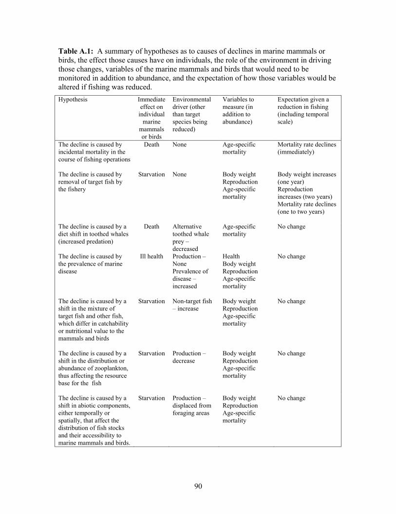
90

Table A.1: A summary of hypotheses as to causes of declines in marine mammals or

birds, the effect those causes have on individuals, the role of the environment in driving

those changes, variables of the marine mammals and birds that would need to be

monitored in addition to abundance, and the expectation of how those variables would be

altered if fishing was reduced.

Hypothesis Immediate

effect on

individual

marine

mammals

or birds

Environmental

driver (other

than target

species being

reduced)

Variables to

measure (in

addition to

abundance)

Expectation given a

reduction in fishing

(including temporal

scale)

The decline is caused by

incidental mortality in the

course of fishing operations

Death None Age-specific

mortality

Mortality rate declines

(immediately)

The decline is caused by

removal of target fish by

the fishery

Starvation None Body weight

Reproduction

Age-specific

mortality

Body weight increases

(one year)

Reproduction

increases (two years)

Mortality rate declines

(one to two years)

The decline is caused by a

diet shift in toothed whales

(increased predation)

Death

Alternative

toothed whale

prey –

decreased

Age-specific

mortality

No change

The decline is caused by

the prevalence of marine

disease

Ill health Production –

None

Prevalence of

disease –

increased

Health

Body weight

Reproduction

Age-specific

mortality

No change

The decline is caused by a

shift in the mixture of

target fish and other fish,

which differ in catchability

or nutritional value to the

mammals and birds

Starvation Non-target fish

– increase

Body weight

Reproduction

Age-specific

mortality

No change

The decline is caused by a

shift in the distribution or

abundance of zooplankton,

thus affecting the resource

base for the fish

Starvation Production –

decrease

Body weight

Reproduction

Age-specific

mortality

No change

The decline is caused by a

shift in abiotic components,

either temporally or

spatially, that affect the

distribution of fish stocks

and their accessibility to

marine mammals and birds.

Starvation Production –

displaced from

foraging areas

Body weight

Reproduction

Age-specific

mortality

No change