Understanding the Interaction Between Blood Flow and an

University of South Florida University of South Florida

Digital Commons @ University of South Florida Digital Commons @ University of South Florida

Graduate Theses and Dissertations Graduate School

10-27-2010

Understanding the Interaction Between Blood Flow and an Understanding the Interaction Between Blood Flow and an

Applied Magnetic Field Applied Magnetic Field

Francy L. Sinatra University of South Florida

Follow this and additional works at: https://digitalcommons.usf.edu/etd

Part of the American Studies Commons, and the Mechanical Engineering Commons

Scholar Commons Citation Scholar Commons Citation Sinatra, Francy L., "Understanding the Interaction Between Blood Flow and an Applied Magnetic Field" (2010). Graduate Theses and Dissertations. https://digitalcommons.usf.edu/etd/3518

This Thesis is brought to you for free and open access by the Graduate School at Digital Commons @ University of South Florida. It has been accepted for inclusion in Graduate Theses and Dissertations by an authorized administrator of Digital Commons @ University of South Florida. For more information, please contact [email protected].

http://scholarcommons.usf.edu/

http://scholarcommons.usf.edu/

https://digitalcommons.usf.edu/

https://digitalcommons.usf.edu/etd

https://digitalcommons.usf.edu/grad

https://digitalcommons.usf.edu/etd?utm_source=digitalcommons.usf.edu%2Fetd%2F3518&utm_medium=PDF&utm_campaign=PDFCoverPages

http://network.bepress.com/hgg/discipline/439?utm_source=digitalcommons.usf.edu%2Fetd%2F3518&utm_medium=PDF&utm_campaign=PDFCoverPages

http://network.bepress.com/hgg/discipline/293?utm_source=digitalcommons.usf.edu%2Fetd%2F3518&utm_medium=PDF&utm_campaign=PDFCoverPages

mailto:[email protected]

Understanding the Interaction Between

Blood Flow and an Applied Magnetic Field

by

Francy L. Sinatra

A thesis submitted in partial fulfillment of the requirements for the degree of

Master of Science in Mechanical Engineering Department of Mechanical Engineering

College of Engineering University of South Florida

Major Professor: Rajiv Dubey, Ph.D. Shiv-Shankar Sundaram, Ph.D.

Rasim Guldiken, Ph.D. Phillip J. Hipol, MSM&AT

Date of Approval: October 27, 2010

Keywords: Magnetization, Static Magnetic Field, Finite Element Model, Pulsatile Blood Flow, Relaxation Time

Copyright © 2010, Francy L. Sinatra

i

Table of Contents

List of Tables ........................................................................................................iv

List of Figures ....................................................................................................... v

Abstract ............................................................................................................... vii

Chapter 1 - Introduction ........................................................................................ 1

1.1 Problem Statement ......................................................................... 1

1.2 Goal of Thesis ................................................................................. 3

1.3 Hypothesis ...................................................................................... 3

Chapter 2 – Background ....................................................................................... 4

2.1 Methods to Measure Blood Flow ..................................................... 4

2.1.1 Thermodilution ...................................................................... 4

2.1.2 Digital Subtraction Angiography ........................................... 5

2.1.3 Electromagnetic Flow Probes ............................................... 6

2.1.4 Doppler Catheter .................................................................. 6

2.1.5 Pulse Oximetry ..................................................................... 7

2.1.6 Laser Doppler Flowmetry ..................................................... 7

2.1.7 Doppler Echocardiography ................................................... 8

2.1.8 Superconducting Quantum Interference Device (SQUID) .. 10

2.1.9 Hall Effect Sensors ............................................................. 10

2.1.10 Impedance Cardiography ................................................... 10

2.1.11 Tomography ....................................................................... 11

2.1.11.1 Ultrafast Computed Tomography ....................... 11

2.1.11.2 Positron-Emission Tomography ......................... 12

2.1.12 Magnetic Resonance Imaging ............................................ 13

2.1.13 Modulated Magnetic Signature of Blood (MMSB) ............... 13

2.2 Magnetism .................................................................................... 15

2.2.1 Magnetization ..................................................................... 16

2.2.2 Magnetic Materials ............................................................. 18

2.2.2.1 Diamagnetic Material............................................ 18

2.2.2.2 Paramagnetic Material ......................................... 19

2.2.2.3 Ferromagnetic Material ........................................ 19

2.2.2.4 Ferrimagnetic Material.......................................... 19

2.2.2.5 Superparamagnetic Material ................................ 20

2.2.3 Magnetic Fluid .................................................................... 20

2.2.3.1 Ferrofluid .............................................................. 21

ii

2.2.3.2 Paramagnetic Solution ......................................... 21

2.2.3.3 Blood .................................................................... 22

Chapter 3 – Experimental Model ........................................................................ 23

3.1 Setup ............................................................................................. 23

3.1.1 Gaussmeter ........................................................................ 24

3.1.2 Permanent Magnets ........................................................... 25

3.1.3 Magnetic Fluids .................................................................. 25

3.1.4 Shielding ............................................................................. 26

3.2 Experimental Trials ....................................................................... 26

3.2.1 Permanent Magnet Characterization .................................. 27

3.2.2 Constant Flow .................................................................... 28

3.2.3 Pulsatile Flow ..................................................................... 28

3.3 Limitations ..................................................................................... 28

3.4 Results .......................................................................................... 29

3.4.1 Permanent Magnet Characterization .................................. 29

3.5 Velocity Trials ................................................................................ 30

3.5.1 Paramagnetic Solution ....................................................... 30

3.5.2 Ferrofluid ............................................................................ 31

3.6 Discussion ..................................................................................... 34

Chapter 4 – Theoretical Model ........................................................................... 37

4.1 Setup ............................................................................................. 37

4.1.1 Governing Equations .......................................................... 37

4.1.1.1 Magnetostatics ..................................................... 38

4.1.1.2 Laminar Flow ........................................................ 39

4.1.2 Geometry ............................................................................ 40

4.1.3 Boundary Conditions .......................................................... 41

4.1.3.1 Magnetostatics ..................................................... 41

4.1.3.2 Laminar Flow ........................................................ 41

4.2 Validation ...................................................................................... 42

4.3 Simulation Trials ............................................................................ 42

4.3.1 Stationary ........................................................................... 43

4.3.2 Transient – Pulsatile Flow .................................................. 44

4.4 Results .......................................................................................... 45

4.4.1 Validation ............................................................................ 45

4.4.2 Magnetostatics ................................................................... 46

4.4.2.1 Single Magnet ...................................................... 46

4.4.2.2 Double Magnet ..................................................... 49

4.4.3 Laminar Flow ...................................................................... 54

4.4.3.1 Stationary ............................................................. 54

4.4.3.2 Transient – Pulsatile Flow .................................... 56

4.4.4 Magnetostatics and Laminar Flow ...................................... 57

4.5 Discussion ..................................................................................... 58

iii

Chapter 5 – Conclusion and Future Work .......................................................... 64

References ......................................................................................................... 67

iv

List of Tables

Table 1 Comparison of current blood flow technologies. .................................... 15

Table 2 Magnetic flux density of the paramagnetic solution. .............................. 30

Table 3 Ferrofluid magnetization values for varying fluid velocities and varying separation values between the permanent magnet and the magnetic sensor. ............................................................................. 31

Table 4 Ferrofluid magnetization for particle concentration of 7.9% by vol. ........ 32

Table 5 Ferrofluid magnetization for particle concentration of 4% by vol. ........... 32

Table 6 Ferrofluid magnetization for a particle concentration of 2% by vol. ........ 33

Table 7 Simulation domain properties ................................................................ 42

v

List of Figures

Figure 1 Reflected signal differences for blood flowing away and towards the Doppler echocardiography probe [42]. .............................................. 8

Figure 2 Pulse rate results captured on an oscilloscope using the MMSB method. ................................................................................................ 14

Figure 3 Electron orbital and spinning motion [57]. ............................................. 16

Figure 4 Graphical illustration of ferromagnetic, ferrimagnetic, paramagnetic and diamagnetic materials [61]. .................................... 18

Figure 5 In-vitro test experimental set-up. .......................................................... 24

Figure 6 5080 F.W. Bell gaussmeter sensor location graphic. ........................... 25

Figure 7 Implemented aluminum shielding ......................................................... 26

Figure 8 Experimental set-up for dual permanent magnet characterization. ...... 27

Figure 9 Dual magnet characterization results, graph of magnetic flux density vs. distance. ............................................................................ 29

Figure 10 Magnetic flux density for dual magnet configuration of 0.125" by 0.5' with varying particle concentration. .............................................. 33

Figure 11 Magnetic relaxation profiles. ............................................................... 36

Figure 12 Finite element model geometry. ......................................................... 40

Figure 13 Comparison between experimental and simulation values of the magnetic flux density with varying distance. ....................................... 46

Figure 14 Single magnet magnetic flux density surface plot ............................... 47

Figure 15 Magnetic flux distance variation with distance for a single magnet along the top boundary of the glass capillary......................... 47

Figure 16 Magnetic flux contribution from blood with a single magnet. .............. 48

vi

Figure 17 Surface plot of the magnetic flux density in the dual magnet configuration.. ..................................................................................... 49

Figure 18 Magnetic flux distance variation with distance for dual magnets along the top boundary of the glass capillary. .................................... 50

Figure 19 Magnetic flux contribution from blood with a dual magnet. ................. 51

Figure 20 Magnetic field variations against the magnetic flux density. ............... 52

Figure 21 Parametric sweep of remnant magnetic flux densities........................ 53

Figure 22 Blood induced magnetic flux density with a remnant magnetic flux. ..................................................................................................... 53

Figure 23 Blood contribution of magnetic flux density with varying mass fraction. ............................................................................................... 54

Figure 24 Surface plot of constant velocity in capillary glass with an input velocity of 0.5 m/s. .............................................................................. 55

Figure 25 Poiseuille flow representation by an arrow plot, observed at the outlet of the capillary tube ................................................................... 56

Figure 26 Constant velocity parametric sweep ................................................... 56

Figure 27 Pulsatile flow parametric sweep. ........................................................ 57

Figure 28 Induced magnetic flux density from blood at a distance of 5mm away from the magnet. ....................................................................... 58

Figure 29 Magnetized particle movement representation of length L in a tube with mean velocity V and Poiseuille flow [76]. ............................ 61

Figure 30 Magnetization distribution with time for particles in Poiseuille flow [76]. ............................................................................................. 62

Figure 31 Magnetization of blood during one heartbeat. .................................... 63

vii

Abstract

Hemodynamic monitoring is extremely important in the accurate

measurement of vital parameters. Current methods are highly invasive or non-

continuous, and require direct access to the patient’s skin. This study intends to

explore the modulated magnetic signature of blood method (MMSB) to attain

blood flow information. This method uses an applied magnetic field to magnetize

the iron in the red blood cells and measures the disturbance to the field with a

magnetic sensor [1]. Exploration will be done by experimentally studying in-vitro,

as well as simulating in COMSOL the alteration of magnetic fields induced by the

flow of a magnetic solution. It was found that the variation in magnetic field is due

to a high magnetization of blood during slow flow and low magnetization during

rapid flow. The understanding of this phenomenon can be used in order to create

a portable, non-invasive, continuous, and accurate sensor to monitor the

cardiovascular system.

1

Chapter 1 - Introduction

1.1 Problem Statement

Circulating blood provides the nourishment (nutrients, oxygen and soluble

factors) needed for supporting life. Hemodynamic monitoring involves keeping

track of oxygen perfusion in tissues in order to prevent ischemia and subsequent

hypoxia (cell death due to lack of oxygen) [2]. Hemodynamic stability is the

proper functioning of the cardiovascular system, being reflected by a blood

pressure of 120 mmHG during the systolic phase and 80 mmHG in the diastolic

phase [3]. Additionally, the beat to beat variability for a healthy adult is

considered to be from 60 to 100 beats/min [4]. Thus, hemodynamic monitoring

involves the accurate measurement of vital parameters of the cardiovascular

system and is common practice in the medical field [5, 6]. It is particularly

important in intensive care units, where continuous hemodynamic monitoring

provides useful information which can help medical personnel predict and

mitigate “early stage” hemodynamic instability, rather than dealing with its after

effects [7]. Measurements commonly used for this purpose include heart rate,

blood pressure, and oxygen saturation. Of these, making beat to beat blood

pressure or volume measurements in a non-invasive and accurate fashion are

the most challenging.

2

Current methods are highly invasive or non-continuous, and often times

require direct access to the patients’ skin. Traditional hemodynamic monitoring is

based on the ability to measure venous and arterial pressure [8]. Changes in

blood pressure often mean late indications of hypoxia due to vasolidation or

vasoconstriction. Thus, pressure can be a misleading late-stage measurement

regarding the hemodynamic condition of a patient [9]. Since the cardiovascular

system is a closed system, every change in a hemodynamic factor triggers

counterbalancing changes in other factors [10]. The current, most popular device

for monitoring the hemodynamic system is the Swan-Ganz catheter which uses

the thermodilution principle to acquire hemodynamic information [11]. This

method is mainly used when patients are exhibiting pronounced hemodynamic

instability. There are other invasive and non-invasive methods which cannot be

utilized for prolonged periods of time, as they are physically inconvenient for the

patient, especially those monitored during strenuous activities.

This study explores a newly reported blood flow monitoring method that

uses an applied magnetic field coupled with a magnetic sensor [1]. COMSOL

Multiphysics modeling and corresponding in-vitro studies are performed to

investigate the alteration of magnetic fields induced by the flow of a magnetic

fluid. The main focus of the project involves understanding the relationship

between the various parameters that affect the magnetization of magnetic

particles within the fluid and thereby the induced magnetic field which can be

measured. These parameters include velocity profile of the solution, magnitude

of applied magnetic field, and magnetic solution concentration. A detailed

3

understanding of this phenomenon portends the design of a portable sensor to

be placed over a patient’s artery, which can non-invasively, continuously, and

accurately monitor critical blood flow properties. Such a sensor can be used in

emergency response vehicles, the ICU, in the field, and at home to aid with early

detection of hemodynamic instability.

1.2 Goal of Thesis

The primary goal of this study is:

• To understand the relationship between the induced magnetic field

created through magnetization of blood analog biomagnetic solution as

well as field parameters.

1.3 Hypothesis

• Variations will exist in the magnetization of the magnetic solution with

particle concentration and applied static magnetic field.

• Variations in the magnetic field will be observed during pulsatile flow of

the magnetic solution.

4

Chapter 2 – Background

2.1 Methods to Measure Blood Flow

Current methods of blood flow monitoring are non-continuous, expensive

and inconvenient, require direct contact of the skin, or are invasive [12-14]. The

most commonly used device in coronary disease units is catheterization of the

pulmonary artery with the Swan-Ganz catheter; which provides continuous

monitoring, but is invasive and causes complications associated with catheter

insertion [15]. Other invasive methods to measure blood flow include digital

subtraction angiography [16], the use of electromagnetic flow probes [17], or

Doppler catheters [18]. Non-invasive methods currently used consist of pulse

oximetry [19-22], Doppler flowmetry [23-26], impedance cardiography [27],

Doppler echocardiography [28], computarized tomography [29], magnetic

resonance imaging, or magnetic sensors such as super quantum interference

devices (SQUID) [30] or Hall effect sensors [31]. The following sections will

describe the various methods of measuring blood flow, along with the

advantages and disadvantages associated with them.

2.1.1 Thermodilution

Thermodilution is the most common method to track coronary blood flow,

highly used since the 1970’s. It involves introducing a Swan-Ganz catheter in the

right coronary sinus [32, 33]. New advances incorporated into the catheter have

5

increased its applications. Fiber optics has allowed for the monitoring of oxygen

saturation levels spectrometrically. In addition, a fast responding thermocouple

and a thermal resistor have been incorporated into the catheter. The

thermocouple indicates the right ventricle ejection fraction and the thermistor,

reveals the cardiac output. Despite its many advantages, several limitations are

associated with the use of thermodilution [17]. The limitations include the lack of

continuous measurements, inability to assess rapid changes in blood flow, and

the failure to estimate perfusion to the right atria or ventricle and to specific

transmural layers. Additionally, the very nature of catheter insertion carries with it

some dangers such as arrhythmia, sepsis, infection, allergic reactions as well as

increased mortality and morbidity [15, 34, 35].

2.1.2 Digital Subtraction Angiography

This method requires the injection of fluorescent contrast media. In digital

subtraction angiography, pre-contrast images are subtracted from the contrasted

images, which aid in visualizing the blood vessels. High spatial resolution is

acquired with this technique; however, the contrast media transit time is slow

which hinders detection of rapid blood flow changes [16]. Absolute blood flow

cannot be determined with this method as it depends on assessment of perfusion

before and after coronary dilation. Several variables that affect the accuracy of

this method include the quantity and method of the contrast injection, effects of

the contrast agent on the blood flow, the protocol for digital angiography

subtraction, and the algorithm used to calculate the changes in perfusion [36-38].

6

2.1.3 Electromagnetic Flow Probes

Electromagnetic flow probes are used to continuously monitor vein bypass

graft blood flow with a millisecond time constant. The electromagnet flow probe is

typically implanted before use, and contact between the vessel wall and the

probe is stabilized using fibrous adhesions. However, when the probe is placed

intra-operatively, major calibration complications. Also, contact with the vessel

can change significantly with pressure alteration and result in erroneous

readings. Even if the probe could be calibrated when used intra-operatively, the

perfusion field is not usually defined thus, limiting the accuracy of the

measurement of blood flow in a graft [39]. Additionally, measurement of coronary

blood flow using the electromagnet flow probe is inherently unsafe since vessel

dissection is required to insert the encircling probe [17].

2.1.4 Doppler Catheter

The Doppler catheter employs a small piezoelectric crystal incorporated

inside the tip of a small probe that is inserted into a catheter. The crystal emits

and receives a signal that reflects off the blood allowing for the detection of blood

velocity. Unlike the electromagnetic flow probe, it is not necessary to encircle the

vessel with the Doppler catheter, and thus perform unsafe vessel dissection [18].

This method makes several assumptions such as a fixed vessel cross-sectional

area, a uniform vessel velocity profile, and a stable angle between the crystal

and the bloodstream. This method can only measure changes in velocity instead

of absolute velocity, which presents a great disadvantage [40, 41]. As mentioned

7

in the thermodilution method, there are again complications associated with the

insertion of a catheter.

2.1.5 Pulse Oximetry

A pulse oximeter measures the saturation of peripheral oxygen in the

blood, also providing a heart rate reading. The principle behind this method

involves the reflection of incident light off red blood cells measured by a photon

sensor. Since this is an optical measurement, the device is limited to use on

fingers, toes, and ear lobes, where interfering tissue absorbance and scattering

is minimal. Furthermore, low signal-to-noise ratio and artifact motion may

constitute significant sources of error and have been noted [20]. Other

confounding factors affecting the accuracy of the pulse oximetry method involve

transducer movement, non-pulsatile vascular bed, peripheral vasoconstriction,

hypothermia, hypotension, anemia, changes in vascular resistance, and

obstructions such as nail polish and tattoos [19]. Studies have also suggested

that finger-probe oximeters may be more accurate than ear-probe, limiting the

versatility of pulse oximetry [22].

2.1.6 Laser Doppler Flowmetry

Another optical method of assessing the microvascular blood perfusion is

Laser Doppler flowmetry. This is done by emitting a single frequency light source

through tissue and processing the frequencies of the scattered light to obtain

blood perfusion. A frequency shift occurs when the light hits the red blood cells in

the blood and bounces back [24, 26]. The disadvantages of this method include

8

long computational time, processing bandwidth, instrument calibration, non-

portability, artifact noise, high cost, and the effect of probe pressure on the skin.

Studies have also recognized interferences when trying to detect vital signs due

to thermal noise, flicker noise, and residual phase [23, 25].

2.1.7 Doppler Echocardiography

In traditional echocardiography, an ultrasound (high frequency) wave is

emitted into the body, and reflected back by the tissues. The probe measures the

change in the returned signal, and it can acquire flow characteristics such as

velocity, direction and turbulence.

Figure 1 Reflected signal differences for blood flowing away and towards the Doppler echocardiography probe [42].

As seen in Figure 1, if the flow is directed away from the emitted signal,

the change in the signal has a lower frequency; when the flow is directed towards

the emitted signal, the reflected signal will have a higher frequency than that

emitted by the probe. This method is highly dependent on the angle the beam is

directed with respect to the blood flow. As shown by the Doppler shift equation,

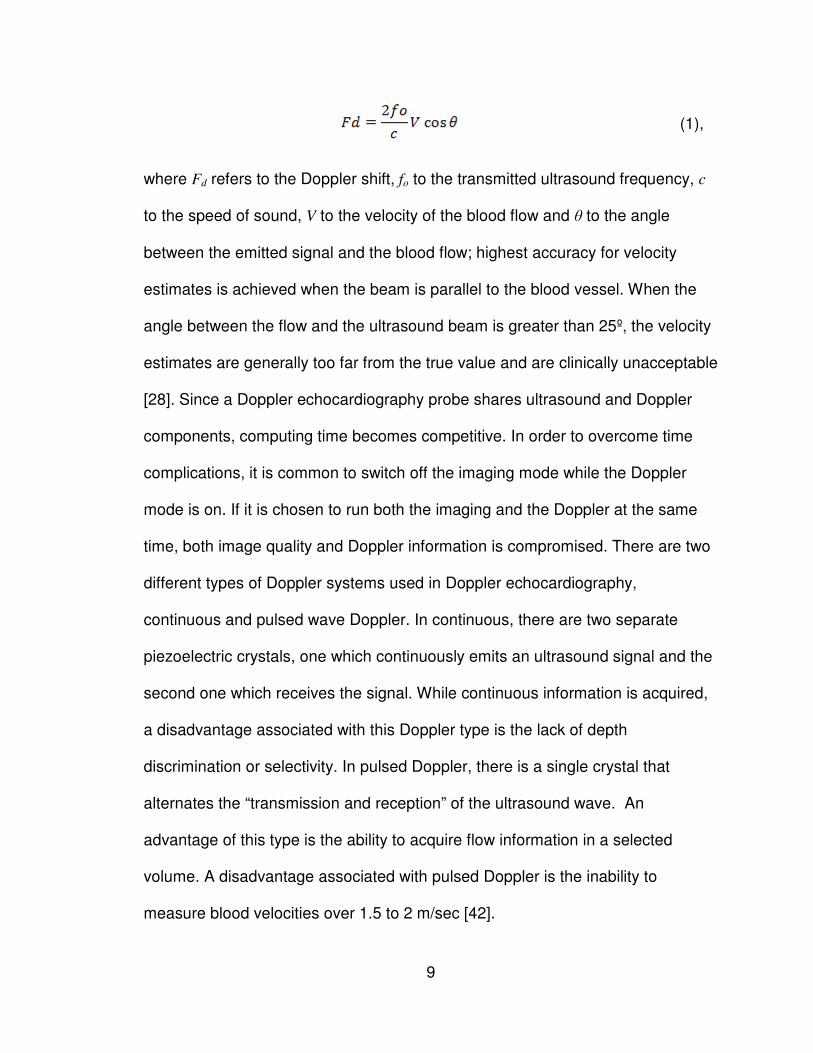
9

(1),

where Fd refers to the Doppler shift, fo to the transmitted ultrasound frequency, c

to the speed of sound, V to the velocity of the blood flow and θ to the angle

between the emitted signal and the blood flow; highest accuracy for velocity

estimates is achieved when the beam is parallel to the blood vessel. When the

angle between the flow and the ultrasound beam is greater than 25º, the velocity

estimates are generally too far from the true value and are clinically unacceptable

[28]. Since a Doppler echocardiography probe shares ultrasound and Doppler

components, computing time becomes competitive. In order to overcome time

complications, it is common to switch off the imaging mode while the Doppler

mode is on. If it is chosen to run both the imaging and the Doppler at the same

time, both image quality and Doppler information is compromised. There are two

different types of Doppler systems used in Doppler echocardiography,

continuous and pulsed wave Doppler. In continuous, there are two separate

piezoelectric crystals, one which continuously emits an ultrasound signal and the

second one which receives the signal. While continuous information is acquired,

a disadvantage associated with this Doppler type is the lack of depth

discrimination or selectivity. In pulsed Doppler, there is a single crystal that

alternates the “transmission and reception” of the ultrasound wave. An

advantage of this type is the ability to acquire flow information in a selected

volume. A disadvantage associated with pulsed Doppler is the inability to

measure blood velocities over 1.5 to 2 m/sec [42].

10

2.1.8 Superconducting Quantum Interference Device (SQUID)

A previous method using a super sensitive magnetic sensor or SQUID has

been used to monitor the heart signal. This method was developed in 1963 by

Baule McFee. The principle behind this method involves the determination of the

magnetic field around the chest area while the magnetic vector of the heart is

recorded. This method is more commonly known as a magneto cardiogram

(MCG) [30]. The magnetic sensors were so sensitive that they often acquired

signal noise from outside sources. Interference problems, combined with the cost

of the magnetic sensor however, have kept this technology from mainstream

medicine.

2.1.9 Hall Effect Sensors

Hall Effect sensors are another way of measuring blood pulse. This

method involves the application of a magnetic field on the body in order to create

the blood polarization. A difference in the magnetic signal is recorded from

electrodes which are placed on the skin around the applied magnetic field.

Unfortunately, this method is very susceptible to noise and interference and

depends on good electrical contact of the electrodes onto the skin [31].

2.1.10 Impedance Cardiography

In impedance cardiography a constant, high frequency, low-amplitude

alternating current is applied to the chest by placing four electrodes, two on the

neck and two on the thorax. The corresponding voltage is measured, which

11

allows for the determination of change in chest impedance. The stroke volume

can be calculated with the measured impedance values by using

(2),

where, SV represents the stroke volume, δ is the actual weight of the patient

divided by the ideal weight, H is the patient’s height, (dZ/dT)max is the maximum

value of the first derivative of the impedance waveform, Zo is the reference

impedance and LVET refers to the left ventricular ejection time [27]. A limitation

associated with the impedance cardiograph is that it tends to consistently

overestimate the stroke volume, by up to ten percent of the true value [43].

2.1.11 Tomography

Tomography is an imaging method that involves creating an image from

its projections. A cross-sectional image is created by illuminating the patient’s

body from various directions and collecting the reflectance data [29]. There are

two main methods used for medical imaging to detect blood flow information,

ultrafast computed tomography and positron-emission tomography.

2.1.11.1 Ultrafast Computed Tomography

Ultrafast computed tomography has been used for the evaluation of

coronary graft bypass [44], the assessment of ventricular function [45, 46],

identification of intracardiac mass and the measurement of myocardial mass [47].

In order to measure blood flow, it is necessary to intravenously inject a contrast

agent (die). The agent is illuminated by exposing the patient to a small dose of

12

radiation (X-ray), and thus flow information is acquired. Specifically, blood flow is

measured by “analysis of contrast medium time-density curves from the

myocardium” [48]. An assumption that is used to simplify the blood flow

calculation is that no venous outflow occurs when the maximum initial slope of

the time-density curve occurs. As a result, if venous outflow does arise, then the

computation of blood flow is greatly underestimated. In contrast, overestimation

of blood flow occurs when the blood vessel that is being imaged is much smaller

than the spatial resolution of the computed tomography scanner. This is due to

volume averaging, which leads to undercutting the of the peak height of the

arterial time-density curve [48].

2.1.11.2 Positron-Emission Tomography

Positron-emission tomography is mainly used to acquire functional and

metabolic information of different organs in the body [49]. In this method, a small

dose of a radio-active isotope is intravenously injected in the body, which is

chosen to be absorbed by a specific tissue. In order to gather blood flow

information, 18F-labeled Fluorodeoxyglucose (FDG) and 18O-labeled water are

used. The targeted area is scanned by a positron-emission tomograph, and the

amount of tracer material absorbed by the cells is measured. Blood flow, as well

as glucose content in the blood is correlated to the FDG uptake by the body [50].

When looking at a positron-emission tomography image, the variation in tracer

material uptake is seen as a variation in color. This method permits accurate

representation of blood flow, even when measuring fast blood velocities. Obvious

13

disadvantages are patient exposure to radio-active materials (in the case of

FDG), cost, and required personnel training in a clinical setting [51].

2.1.12 Magnetic Resonance Imaging

Soft tissue can be imaged with the use of magnetic resonance imaging

(MRI), by exposing the body to a strong magnetic field and a radio frequency

signal. The hydrogen atoms in the body align due to the magnetic field.

Excitement with the radio frequency perturbs the alignment, and the protons in

the body respond by sending a signal as they lose energy which is picked up by

a transmitter. The response signal emitted by the hydrogen protons is unique to

various tissues, which creates the contrast image in an MRI [52]. To calculate

blood flow, a specific radio frequency is used which excites the hydrogen protons

in the blood. In MRI, there is a correlation between blood velocity and T1

relaxation [53]. This parameter refers to the time it takes for the hydrogen protons

to demagnetize (random atom alignment). With the use of the T1 relaxation time

and the signal intensity, it is possible to determine blood flow characteristics [54].

While using MRI is an accurate method for acquiring blood flow, it is very

expensive and requires the use of very specialized equipment.

2.1.13 Modulated Magnetic Signature of Blood (MMSB)

This novel method was published in the International Conference of

Biomedical Engineering (ICBME) in 2009 by Phua et al [1]. It entails placing a

small permanent magnet and a magnetic sensor on top of a major artery; and

capturing the blood pulse by measuring the disturbance created in the magnetic

14

field by the pulsatile motion of blood. The results gathered using this method can

be seen in Figure 2, where a clear signal representing the diastolic and systolic

phases of the heart can be seen. This is the first method that has been

presented, which could be used in order to create a sensor that is portable and

can provide non-invasive and continuous tracking of the cardiovascular system.

The principle behind this method is not well understood, and should be further

investigated to acquire a better understanding of the magnetic contribution of

pulsed blood when flowing underneath an applied field.

Figure 2 Pulse rate results captured on an oscilloscope using the MMSB method [1].

Table 1 serves as a comparison between the commonly used methods to

capture blood flow and pulse and MMSB. Most methods are non-continuous and

non-portable, requiring expensive equipment and the use of trained personnel.

15

Table 1 Comparison of current blood flow technologies.

Method Continuous Portable Non-invasive

Thermodilution ��

Subtraction Angiography ��

��

Electromagnetic Flow

Probe

Doppler Catheter ��

Doppler Echocardiography ��

��

Laser Doppler Flowmetry ��

��

Impedance Cardiography

��

Tomography

��

Pulse Oximetry

��

MRI

��

MMSB ��

2.2 Magnetism

Magnetism is the response of a material to a magnetic field [55]. In this

phenomenon, a magnetic material will exert an attractive or repulsive force on

16

other magnetic materials [56]. The change of magnetic energy in a given volume

is what creates a magnetic field. A magnetic moment is produced by the spinning

and orbital motion of an electron.

Figure 3 Electron orbital and spinning motion [57].

The orbital motion is related to the movement of the electron around its

nucleus. The electron spinning motion is the rotation of the electron around its

own axis. Both of these movements contribute to the magnetic behavior seen in

magnetic materials. Higher magnetization is seen with a greater magnetic

moment alignment of the atoms [57]. As seen in Figure 3, the magnetic moment

is always around the atom’s rotational axis.

2.2.1 Magnetization

Magnetization is the amount of magnetic moment per volume possessed

by a material [58]. The magnetic moment is the tendency of a particle to align

with a magnetic field. The relationship between magnetic moment and

magnetization is shown by

17

(3),

where M is the total magnetization in Amperes/meter (A/m), N is the number of

magnetic moments in the sample and V is the volume of the sample in m3.

Magnetic field is a title used interchangeably for the fields produced by the

magnetic flux density B and the material’s magnetic field H. The difference

between these two fields, is that the B field is generated by the free electrons,

and the H field is generated by bound electrons in a material.

Magnetization relates to a materials magnetic field H, through a constant

called magnetic susceptibility χ, which is material specific (Eq. 4). Since χ is unit

less, the units for H are A/m as well.

(4)

Furthermore, the magnetic flux density B can be inferred by knowing a

material’s magnetization and magnetic field H. This relationship is shown by

(5),

where B is the magnetic flux density measured in Gauss and µ0 is the

permeability of free space with a value of 1.25663e-6 in SI units [59].

These equations describe the basic magnetic behavior of various

materials, and provide the basis for understanding the physics behind the

simulations.

18

2.2.2 Magnetic Materials

Magnetic atoms are those that carry a permanent magnetic moment.

Materials are made by an assembly of atoms, which can either be non-magnetic

or magnetic. A material will have different magnetic behavior as well as total

magnetization, depending on the type of atoms. The main types of magnetic

materials are diamagnetic materials, paramagnetic materials, ferromagnetic

materials, ferrimagnetic materials, and superparamagnetic materials [60]. A brief

description of each will be presented below (Figure 4).

Figure 4 Graphical illustration of ferromagnetic, ferrimagnetic, paramagnetic and diamagnetic materials [61].

2.2.2.1 Diamagnetic Material

Diamagnetic materials are only composed of non-magnetic atoms. When

the material is exposed to a magnetic field, the magnetization of these materials

19

is very weak and is opposite to that of the applied magnetic field. This effect is

due to the change of the electronic orbital motion due to the magnetic field. The

magnetic susceptibility of these materials is usually negative and on the order of

10-5.

2.2.2.2 Paramagnetic Material

Paramagnetic materials are composed of magnetic atoms that are

randomly aligned. When the material is exposed to an external magnetic field,

the direction of the moments is momentarily aligned. A magnetization that is

parallel to the direction of the applied field is created, which adds to total field.

The magnetic susceptibility of these materials is usually positive and on the order

of 10-3 to 10-5.

2.2.2.3 Ferromagnetic Material

Ferromagnetic materials have magnetic atoms that produce large

magnetic moments. When a virgin ferromagnetic material is exposed to an

applied magnetic field, the atoms permanently align. This creates a permanent

magnetization, which is parallel to the applied magnetic field.

2.2.2.4 Ferrimagnetic Material

Ferrimagnetic materials are comprised of atoms that have unequal

adjacent magnetic moments aligned in opposite directions. When exposed to an

applied magnetic field, a permanent magnetization is seen similar to that of

ferromagnetic materials, if the material’s temperature is under the Curie

temperature. Below the Curie temperature, the magnetization exhibited in the

20

ferrimagnetic material is permanent. Above the Curie temperature, thermal

agitation can overcome the magnetization forces and randomize the magnetic

moments. Ferrimagnetic materials are more temperature dependent and they

can achieve much higher magnetization values.

2.2.2.5 Superparamagnetic Material

Superparamagentic materials behave similar to paramagnetic materials.

Instead of the individual atoms aligning to an applied magnetic field, the magnetic

moment of the entire crystalline solution is aligned to the field. When there is no

applied magnetic field, the thermal fluctuations are enough to maintain the net

magnetization of superparamagnetic materials equal to zero.

2.2.3 Magnetic Fluid

A magnetic fluid is a solution that contains magnetic particles suspended

in a carrier fluid. In order to ensure an even dispersion of the particles in the

carrier fluid and, avoid agglomeration or particle settling, a surfactant or coatings

are used. A coating has to be matched to the carrier fluid, and overcome the Van

der Waals forces and magnetic forces in order to prevent particle agglomeration

[57]. The most common magnetic fluids are ferrofluids and paramagnetic

solutions. Blood is also considered a magnetic fluid, which has paramagnetic

properties. The following sections contain brief descriptions of ferrofluids,

paramagnetic solutions and blood.

21

2.2.3.1 Ferrofluid

In a ferrofluid, the particles size can vary from 10 nm – 50 nm in diameter,

and are usually made out of magnetite or ferrite. Ferrofluids contain from 1% to

5% of magnetic particles per volume, 10% surfactant, and the remainder is

carrier fluid. In the absence of a magnetic field, the magnetic moments of the

particles are randomly aligned, such as in a paramagnetic material, and the net

magnetization of the solution is zero. A ferrofluid contains superparamagnetic

particles [62]. When a ferrofluid is exposed to an applied magnetic field, the

magnetic particles are instantly magnetized, meaning their magnetic moments

instantly align with the field lines. The magnetic forces that hold a ferrofluid in

place are proportional to the magnetic particle magnetization and the applied

magnetic field. If the ferrofluid is exposed to a weak magnetic field, thermal

energy from agitation of the solution overcomes the magnetic forces that hold the

ferrofluid in place, and the particles randomly disperse.

2.2.3.2 Paramagnetic Solution

In a paramagnetic solution, the particle diameter usually varies from 1 µm

to 30 µm. Paramagnetic solutions contain magnetic beads that possess a ferrite

core of nanometer size, with a shell made out of polystyrene, which increases the

particle size to the micrometer range. These particles are usually commercially

for drug targeting such as in magnetic separation of polypeptides. The

polystyrene shell is usually covered with an antibody or protein, to promote

binding to various polypeptides. The paramagnetic solutions typically contain

from 2.5% to 5% particles by volume, and the remainder of the solution is the

22

mixture of a surfactant with deionized water. As with ferrofluids, when the

solution is exposed to a magnetic field, the magnetic moments of the ferrite cores

instantly align with the field lines. The strength of the magnetization of

paramagnetic particles is less than that of a ferrofluid, but it is also proportional to

the applied magnetic field.

2.2.3.3 Blood

Blood is mainly composed of plasma, which carries proteins, platelets, red

and white blood cells. Red blood cells contain a protein called hemoglobin which

has a high affinity for iron. The average diameter of a red blood cell is between

4.0 µm to 4.5 µm. The average hemoglobin iron concentration is 17 % wt by

volume for males and approximately 15% wt by volume for females [63]. The

density of blood has been published to be 1050 kg/m3 and the dynamic viscosity

0.0035 Pa.s [64]. Blood has been recorded to have different magnetic

susceptibility values depending on its oxygenation state. Deoxygenated blood,

such as that which travels in veins towards the heart, behaves as a paramagnetic

solution and has a magnetic susceptibility of 3.5x10-6. Oxygenated blood, which

is found in arteries and is pumped from the heart, has diamagnetic properties,

with a magnetic susceptibility of -6.67x10-7 [65-67]. The magnetic relaxation of

blood has been experimentally measured to be in the order of a few seconds,

meaning that it will take at least a second for blood to reach its equilibrium

magnetization when exposed to a magnetic field [67, 68].

23

Chapter 3 – Experimental Model

The main purpose of this study is to verify and understand the method of

continuous blood flow monitoring using an applied magnetic field coupled with a

magnetic sensor. This method was first developed by Phua et al [1], and places

an applied magnetic field in the path of an artery. The in vitro experimentation

developed to study the MMSB method is described in the following section.

Further sections in this chapter include the limitations of the experimental set-up

and the results acquired using a ferrofluid and a paramagnetic solution.

3.1 Setup

The experimental set-up used for the in-vitro model is shown in Figure 5.

A Harvard Apparatus PHD 2000 programmable syringe pump was used to flow

the magnetic particles through a glass capillary tube 2.5 mm in diameter. Since

the MMSB method has reported to magnetize the blood in the radial artery, a

capillary tube diameter was chosen to appropriately mimic this condition. A

permanent magnet configuration was suspended around the capillary tube, to

apply a magnetic field on the fluid. Magnetic flux readings were made with the

transverse probe of a 5080 F.W. Bell gauss / teslameter. The flow of the

magnetic particles went from the syringe pump, through the glass capillary, and

finally to a specimen collection container.

24

Figure 5 In-vitro test experimental set-up. (1) is a PHD 2000 Harvard Apparatus programmable syringe pump, (2) is a 5080 F.W. Bell gauss / teslameter, (3) is the gaussmeter transverse probe, (4) is the specimen

collection container, (5) is the permanent magnet configuration and (6) is the glass capillary.

3.1.1 Gaussmeter

The gaussmeter used to gather the magnetic flux readings is the 5080

F.W. Bell meter. The transverse probe of the gaussmeter has a Hall effect sensor

placed 0.9mm from the edge (Figure 6), and positioned so that it will measure

magnetic flux lines perpendicular to the flat side of the probe. A Hall Effect

sensor consists of a Hall generator that has a constant current flowing through it.

When the Hall generator is exposed to a magnetic field, the magnetic flux lines

bend the current to one edge, creating a voltage differential. Generally, there is a

linear relationship between the generated voltage and the magnetic flux field [69].

The gaussmeter has a measurement range from 0.01 mT to 2.999 T. The

resolution of the readings varies depending on the measurement range that is

being used. A range of 0 G to 300 G has a resolution of 0.1 G, a measurement

range of 300 G to 3 kG has a resolution of 1 G and a measurement range of 3

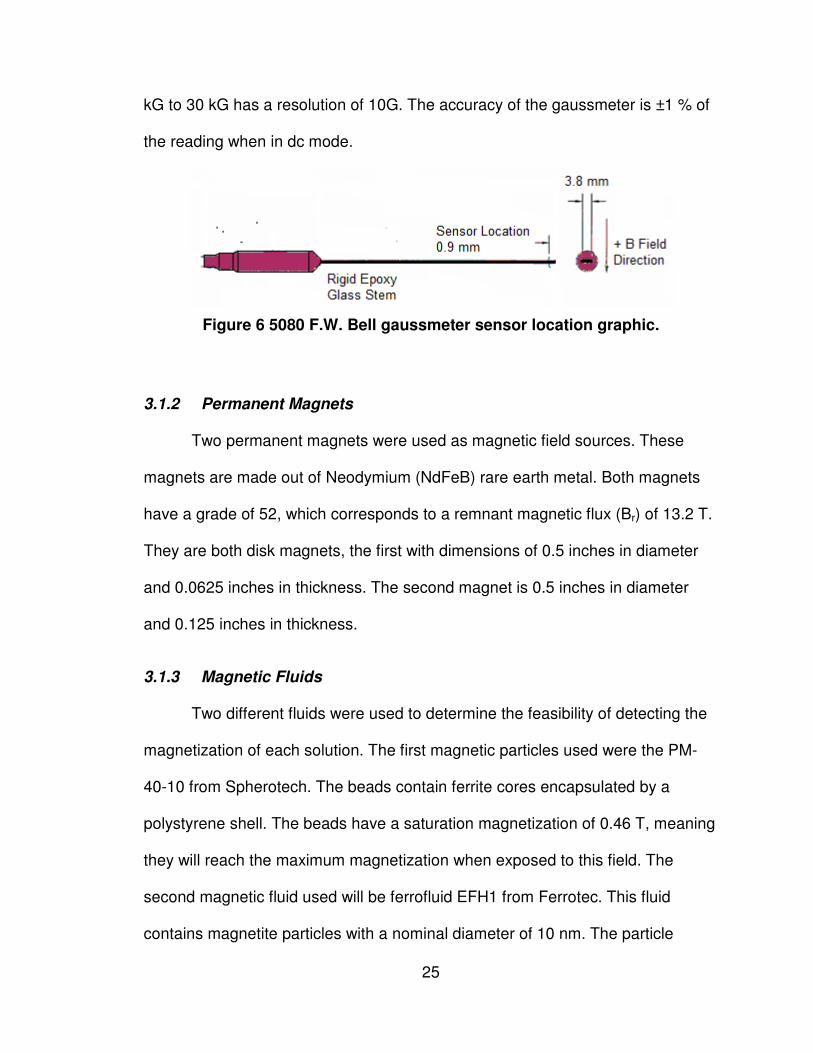
25

kG to 30 kG has a resolution of 10G. The accuracy of the gaussmeter is ±1 % of

the reading when in dc mode.

Figure 6 5080 F.W. Bell gaussmeter sensor location graphic.

3.1.2 Permanent Magnets

Two permanent magnets were used as magnetic field sources. These

magnets are made out of Neodymium (NdFeB) rare earth metal. Both magnets

have a grade of 52, which corresponds to a remnant magnetic flux (Br) of 13.2 T.

They are both disk magnets, the first with dimensions of 0.5 inches in diameter

and 0.0625 inches in thickness. The second magnet is 0.5 inches in diameter

and 0.125 inches in thickness.

3.1.3 Magnetic Fluids

Two different fluids were used to determine the feasibility of detecting the

magnetization of each solution. The first magnetic particles used were the PM-

40-10 from Spherotech. The beads contain ferrite cores encapsulated by a

polystyrene shell. The beads have a saturation magnetization of 0.46 T, meaning

they will reach the maximum magnetization when exposed to this field. The

second magnetic fluid used will be ferrofluid EFH1 from Ferrotec. This fluid

contains magnetite particles with a nominal diameter of 10 nm. The particle

concentration is 7.9% by

The ferrofluid’s magnetic susceptibility is

blood. Hence, it is assumed that the

stronger, which decreases the sensitiv

measuring device. The ferrofluid has

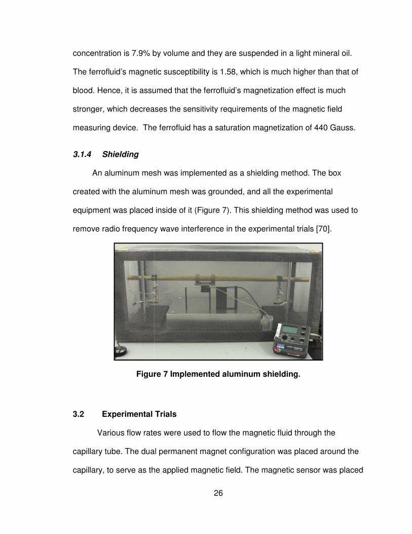
3.1.4 Shielding

An aluminum mesh was implemented as a shielding method. The box

created with the aluminum mesh was grounded, and all the experi

equipment was placed inside

remove radio frequency wave interference in the exp

Figure

3.2 Experimental Trials

Various flow rates were used to flow the magnetic fluid

capillary tube. The dual

capillary, to serve as the

26

by volume and they are suspended in a light mineral oil.

magnetic susceptibility is 1.58, which is much higher than that of

blood. Hence, it is assumed that the ferrofluid’s magnetization effect is much

stronger, which decreases the sensitivity requirements of the magnetic field

The ferrofluid has a saturation magnetization of 440 Gauss.


created with the aluminum mesh was grounded, and all the experi

equipment was placed inside of it (Figure 7). This shielding method was used to

remove radio frequency wave interference in the experimental trials

Figure 7 Implemented aluminum shielding.

Experimental Trials

Various flow rates were used to flow the magnetic fluid through the

tube. The dual permanent magnet configuration was placed around the

, to serve as the applied magnetic field. The magnetic sensor

volume and they are suspended in a light mineral oil.

which is much higher than that of

effect is much

ity requirements of the magnetic field

a saturation magnetization of 440 Gauss.


created with the aluminum mesh was grounded, and all the experimental

shielding method was used to

erimental trials [70].

through the

placed around the

magnetic field. The magnetic sensor was placed

at various distances away from the permanent magnet, also on top of the

capillary tube. Figure 5

3.2.1 Permanent Magnet Characterization

The magnetic field

dual magnet configuration (

center of the two magnets, and the field was m

The magnet configuration was moved away from the probe

Equation 6 describes the magnetic field at the center between both magnets

along the vertical centerline, as a function of separation distance.

B is the magnetic

magnetic flux in G. x1 = (d/2

from the center point, along the vertical centerline of both magnets and

separation distance between the

permanent magnet in cm and

Figure 8 Experimental set

Horizontal centerline

27


5 shows the experimental set-up.

Permanent Magnet Characterization

magnetic field was measured along the horizontal centerline

configuration (Figure 8). The transverse probe was plac

center of the two magnets, and the field was measured starting from t

The magnet configuration was moved away from the probe at intervals of 5 mm.

the magnetic field at the center between both magnets

along the vertical centerline, as a function of separation distance.

is the magnetic field in G, Br is the permanent magnet’s remnant

= (d/2 – x) and x2 = (d/2 + x) where x is the point of interest

along the vertical centerline of both magnets and

between the magnets (Figure 8). R is the radius of the disk

permanent magnet in cm and T is the thickness of the permanent magnet in cm.

Experimental set-up for dual permanent magnet characterization

x = 0

Travel direction up to x = 2 cm

Horizontal centerline

Vertical centerline

Separation distance


al centerline of the

placed at the

starting from the center.

at intervals of 5 mm.

the magnetic field at the center between both magnets

(6)

gnet’s remnant

point of interest

along the vertical centerline of both magnets and d is the

is the radius of the disk

is the thickness of the permanent magnet in cm.

l permanent magnet characterization.

28

3.2.2 Constant Flow

The input flow rate from the syringe pump is constant during these

experimental trials. The flow rates were varied starting at 20 ml/min, every 10

ml/min until reaching 90 ml/min. These flow rates represent the upper and lower

limits the syringe pump is capable of producing. They correspond to fluid

velocities of 0.06 m/s to 0.3 m/s. The magnetic field produced by the permanent

magnet configuration was also varied, by changing the geometry and strength of

the magnets used. The various magnets used were described in section 3.1.2.

3.2.3 Pulsatile Flow

To emulate the pulsed flow the heart produces, the Harvard Apparatus

syringe pump was programmed to create intervals where the magnetic fluid is

flowing at maximum velocity, followed by no flow for 10 seconds. The fluid profile

is not sinusoidal, but a square wave. The maximum velocity and the permanent

magnet strength were also varied as described during the constant flow trials in

section 3.2.2.

3.3 Limitations

• The magnetic fluid used does not reflect the same behavior as blood,

since oxygenated blood behaves as a diamagnetic material and both the

ferrofluid and the Spherotech solution behave as paramagnetic solutions.

No commercially available diamagnetic solutions were found that would

have a greater magnetic susceptibility than blood.

29

• Magnetic solution magnetization signal is limited by the sensitivity of the

gaussmeter, very small signals are not detected and overpowered by the

ambient noise.

• The simulation of pulsatile flow is limited by the syringe pump, and is

replicated as a square wave instead of a sine wave.

3.4 Results

In this section the results from the experimental trials are discussed. First

the permanent magnet characterization will be addressed, followed by the

outcomes seen during the velocity trials using a paramagnetic solution and a

ferrofluid.

3.4.1 Permanent Magnet Characterization

Characterizations were done to the permanent magnet configuration using

the 0.5 inch in diameter by 0.0625 inch in thickness magnets (Figure 9).

Figure 9 Dual magnet characterization results, graph of magnetic flux density vs. distance.

-100

0

100

200

300

400

500

600

0 0.5 1 1.5 2

Ma

gn

eti

c F

lux

De

nsi

ty (

G)

Distance (cm)

Dual Magnet

30

Equation 6 was used to compare the accuracy of the magnetic flux density

at the center of both magnets. Equation 6 yields a value of 513.4 G and the

measured value was 497.2G. There is little error between the experimental and

calculated values, indicating proper measurement of the magnetic field by the

gaussmeter.

3.5 Velocity Trials

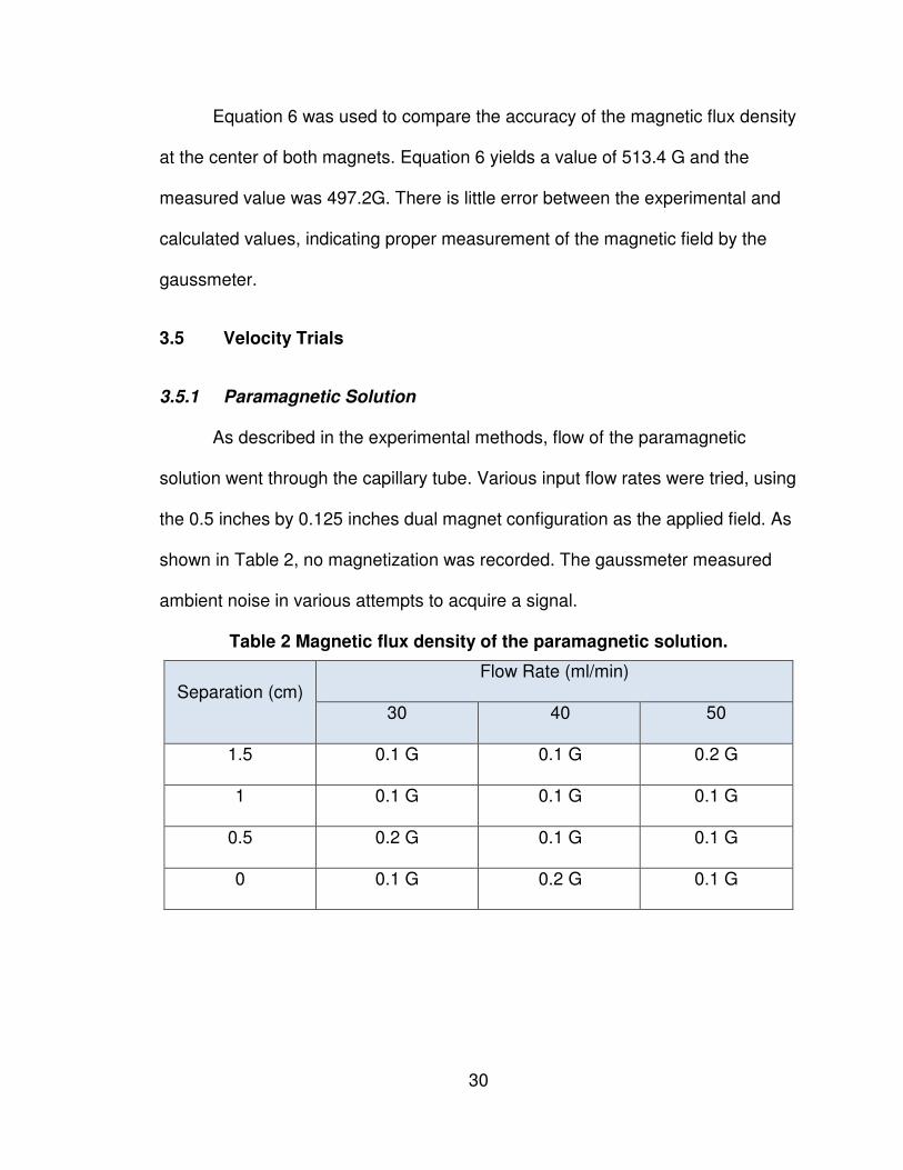
3.5.1 Paramagnetic Solution

As described in the experimental methods, flow of the paramagnetic

solution went through the capillary tube. Various input flow rates were tried, using

the 0.5 inches by 0.125 inches dual magnet configuration as the applied field. As

shown in Table 2, no magnetization was recorded. The gaussmeter measured

ambient noise in various attempts to acquire a signal.

Table 2 Magnetic flux density of the paramagnetic solution.

Separation (cm) Flow Rate (ml/min)

30 40 50

1.5 0.1 G 0.1 G 0.2 G

1 0.1 G 0.1 G 0.1 G

0.5 0.2 G 0.1 G 0.1 G

0 0.1 G 0.2 G 0.1 G

31

3.5.2 Ferrofluid

The input flow rate for the ferrofluid started from 20 mil/min to 90 mil/min

with 10 mil/min intervals. Three magnet configurations were used, two dual

magnets using both permanent magnets described in section 3.1.2 and a single

magnet with thickness of .0625 and diameter of .5 inches. There was no

correlation between increasing velocity and measured magnetic field (Table 3).

Table 3 Ferrofluid magnetization values for varying fluid velocities and varying separation values between the permanent magnet and the

magnetic sensor.

Separation (cm) Flow Rate (ml/min)

30 40 50

1.5 3.6 G 3.6 G 3.6 G

1 - 8.7 G - 8.7 G - 8.7 G

0.5 18 G 18 G 18 G

The results for the variation in magnetization with distance for the different

applied magnetic fields are summarized in Table 4. These magnitudes were

gathered with a ferrofluid particle concentration of 7.9 % by volume. Increase in

the applied magnetic field lead to a greater contribution of the field from the

ferrofluid; confirming the superparamagnetic behavior of the magnetite particles.

There is an inverse correlation between the measured magnetic field and the

separation distance from the permanent magnets. Greater separations lead to a

low field, whereas small separations lead to a larger field. Furthermore, tests

were also run with decreased particle concentration values of 4% and 2%

32

particles by volume (Figure 10). Halving the particle concentration yields half the

magnetic field contribution by the ferrofluid (Table 5 and Table 6).

Table 4 Ferrofluid magnetization for particle concentration of 7.9% by vol.

Separation

(cm)

0.5’x0.125’ Dual

Magnets

0.5’x0.0625’ Dual

Magnets

0.5’x0.0625’ Single

Magnet

B Field

(no fluid)

B Field

of fluid

B Field

(no fluid)

B Field

of fluid

B Field

(no fluid)

B Field

of fluid

1.5 24.5 G 3.6 G 10.4 G 2.5 G 42.2 G 5.2 G

1 - 79.3 G - 8.7 G - 17.5 G - 2.7 G 106.7 G 10.1 G

0.5 253.7 G 18 G 192.9 G 16 G 430.1 G 19 G

Table 5 Ferrofluid magnetization for particle concentration of 4% by vol.

Separation

(cm)

0.5’x0.125’

Dual Magnets

0.5’x0.0625’

Dual Magnets

0.5’x0.0625’

Single Magnet

Measured

Field of Fluid

Measured Field

of Fluid

Measured

Field of Fluid

1.5 1.7 G 1.2 G 2.6 G

1 - 4.4 G - 1.3 G 5.1 G

0.5 7.9 G 8 G 9.6 G

33

Table 6 Ferrofluid magnetization for a particle concentration of 2% by vol.

Separation

(cm)

0.5’x0.125’

Dual Magnets

0.5’x0.0625’

Dual Magnets

0.5’x0.0625’

Single Magnet

Measured

Field of Fluid

Measured Field

of Fluid

Measured Field

of Fluid

1.5 0.9 G 0.6 G 1.2 G

1 - 2.3 G - 0.7 G 2.6

0.5 4 G 4 G 4.8 G

Figure 10 Magnetic flux density for dual magnet configuration of 0.125" by 0.5' with varying particle concentration.

Additionally, the ferrofluid was pulsed using the syringe pump imitating a

square wave profile. A volume of 2 ml of the ferrofluid was flown at a maximum

velocity of 40 ml/min, and then the fluid was paused for ten seconds. No pulsed

-15

-10

-5

0

5

10

15

20

0 0.5 1 1.5 2

Ma

gn

eti

c F

lux

De

nsi

ty (

G)

Distance (cm)

Concentrations vs. Magnetic Flux

7.9 % concentration

4 % concentration

2 % concentration

34

effect was recorded in the magnetic field induced by the ferrofluid. This may be

due to the magnetic relaxation of the ferrofluid. If the demagnetization time is too

fast, then probing for the magnetic field at too great of a separation will not yield

any effects from the magnetization of blood. In contrast, if the demagnetization

time is too slow, then probing for the magnetic field too close to the permanent

magnet will yield a constant magnetization.

3.6 Discussion

The permanent magnet characterizations agreed well with the calculated

values using equation 6. There is an exponential growth in the magnetic field with

decreased separation distance, with the exception at 1 cm, where a decrease in

the magnetic field is observed. This trend may be explained by a change in the

magnetic field lines when getting close to the edge of the permanent magnets.

While performing the experimental trials with the concentration, there was a

decrease in the induced magnetic field by the ferrofluid with decreased particle

concentration. This agrees well with the fundamentals of magnetism; less

amount of particles suspended in the ferrofluid leads to fewer magnetic moments

aligning to the field, which creates a lower magnetic field. Lastly, the lack of

pulsatile nature in the magnetic field when pulsing the ferrofluid may be due to a

fast magnetization time [71]. The ferrofluid is instantly magnetized, whether it

flows by the magnet or sits stationary under it, and thus results in a constant

magnetization regardless of the flow profile of the fluid. Figure 11 shows various

profiles that may occur depending on the magnetic relaxation of the particles. It is

35

desired to have a magnetization profile as in Figure 11 (A), which indicates the

demagnetization of the magnetic particles occurs within the distance of the

permanent magnet. If the magnetization time is very fast, then the solution will

remain magnetized regardless of the profile of the fluid, and appear as a constant

magnetization on the magnetic sensor (B). If the demagnetization time is too

rapid, then the particles will lose magnetization before reaching the magnetic

sensor (C).

36

Figure 11 Magnetic relaxation profiles.

37

Chapter 4 – Theoretical Model

To further understand the interactions between magnetic fluids and an

applied magnetic field, a finite element model using COMSOL Multiphysics 4.0a

was created [72]. The Navier-Stokes relations were used to solve for the velocity

profile of the magnetic fluid. Maxwell’s equations, along with Gauss’ and

Ampere’s Laws were used to determine the magnetic field from the permanent

magnet and the magnetic fluid. The model described below is a derivation of a

previously established model by COMSOL to describe the interactions between a

magnetic fluid and a permanent magnet to use for drug targeting studies. The

finite element model setup, validation, the simulations performed and the

observed results are discussed in this chapter.

4.1 Setup

The following sections include descriptions of the finite element model,

including the governing equations used, the specific geometry, and the boundary

conditions.

4.1.1 Governing Equations

The governing equation for the fluid model is the time-dependent Navier-

Stokes equation [73] and, for the magnetostatic model, the Maxwell-Ampere

38

equation [59]. The next sections will briefly introduce these equations and the

formulation used for the different domains in the finite element model.

4.1.1.1 Magnetostatics

• Maxwell-Ampere’s law:

(7)

• Gauss’ law:

(8)

• Curl of vector field:

(9)

• Continuity equations:

(10)

(11)

(12)

• Magnetic fluid magnetization [74]:

(13)

(14)

39

where,

• H is the magnetic field in Amps/meter

• B is the magnetic flux density in Tesla

• �� is the free permeability of space

• ��,�� is the relative permeability of the magnet

• M is the magnetization in Amps/meter

• Χ is the magnetic susceptibility

• Az is the vector potential in the z direction in Volts*second/meter

4.1.1.2 Laminar Flow

• Navier-Stokes:

(15)

• Continuity equation:

(16)

where,

• ρ is the density in kilogram/meter3

• u is the velocity in meter/second

• η is the dynamic viscosity in Pascals*second

• P is the pressure in Pascals

• F is the force on the fluid in Newtons

40

4.1.2 Geometry

The geometry used in the 2D finite element model is shown in Figure 12.

The green boundaries encompass the magnetic fluid. The blue boundaries refer

to the permanent magnet. Sufficient space for dissipation of the magnetic flux

lines is given by creating a large domain with air surrounding the magnets and

the fluid.

Figure 12 Finite element model geometry.

It is of interest to investigate the difference between the magnetization of

the magnetic fluid when using one magnet as done by Phua et al. [1] and when

using two parallel magnets. The geometry for the single magnet simulations is

identical to that shown for the dual magnet simulations, with the exception of the

removal of the bottom permanent magnet. It is assumed that the magnetic field

between the two parallel magnets will be more uniform, thus having a greater

41

effect with the alignment of the magnetic moments of the magnetic fluid.

Comparison of the results between the simulations using two parallel magnets

and a single magnet were performed.

4.1.3 Boundary Conditions

Proper boundary conditions are declared to find solutions to the model.

Descriptions of the boundary conditions are explained below.

4.1.3.1 Magnetostatics

• Magnetic Insulation: A = 0; Magnetic potential is equal to zero in the

normal direction.

o Boundary condition selected for all boundaries surrounding the

domain containing air.

• Continuity: n x (H1 – H2) = 0; Signifies continuity of the tangential

component of the magnetic field.

o Boundary condition selected for all boundaries surrounding the

magnets and the fluid, with exception of the fluid inlet and outlet.

4.1.3.2 Laminar Flow

• No Slip: u = 0; Refers to the non-slip condition between the fluid and rigid

walls.

o Boundary condition selected for the top and bottom boundary of

the fluid.

• Inlet: u = C; Velocity at the inlet is equal to a constant C.

o Boundary condition selected for the inlet of the fluid.

42

• Outlet: P = 0; Pressure at outlet is equal to zero, signifies an open

boundary.

o Boundary condition selected for the outlet of the fluid.

4.2 Validation

To establish the validity of the finite element model, a simulation using the

dual magnets of 0.5” diameter and 0.125” thickness was performed. The

magnetic flux density was probed at the horizontal centerlines between the

magnets (Figure 8), and compared to experimental results.

4.3 Simulation Trials

The trials simulated the behavior between a magnetic fluid and an applied

magnetic field. There are four main domains set-up in the finite element model.

One corresponds to the air, two to Neodymium Iron Boron permanent magnets

and one to the magnetic fluid. The material properties used in each of the

domains are listed below.

Table 7 Simulation domain properties

Domains Ρ (kg/m3) µ (Pa.s) Χ σ εr

Air N/A N/A 1 0 1

Neodymium Iron Boron

Magnet N/A N/A 1.05 0 1

Magnetic

Fluid

Ferrofluid 1210 0.006 1.56 0 1

Blood 1050 0.0035 -0.667e-6 0 1

43

A parametric study was performed in the finite element model by varying

three different properties. The parameters being varied for the fluid are the profile

of the input velocity along with the input velocity. The magnetostatics domain

also has parameters that are being varied, which are the strength of the

permanent magnet or remnant magnetic flux and the magnetic particle mass

fraction. All parametric simulations will be done using the properties of blood,

since it is of interest to find out how the change in the various parameters affects

the creation of a blood flow sensor. The values were varied for the mass fraction

of the magnetic particles from 0 kg/kg to 1 kg/kg with 0.1 kg/kg intervals.

Additionally, the applied magnetic field was varied by having permanent magnets

with remnant magnetic flux starting at 0 T to 2 T at 0.1 T intervals. The model

was probed for the magnetic flux at various points at the top boundary of the

fluid. The following sections describe the simulations performed for validation

purposes of the finite element model along with the fluid profile variations

implemented in the fluid model.

4.3.1 Stationary

The inlet velocity during the stationary trials is equal to a constant number.

This indicates that the flow profile is uniform, and is constant with time. The inlet

velocity was varied from 0 m/s to 1 m/s with 0.1 m/s intervals. The range for the

velocity variations was chosen, since 0.5 m/s is the average velocity value for

blood flowing in the radial artery.

44

The solver used for this model is the MUMPS direct solver. This solver is a

fast solving algorithm, which is usually necessary when trying to use cluster

computation.

4.3.2 Transient – Pulsatile Flow

The input velocity for the time dependent model is a function of time and it

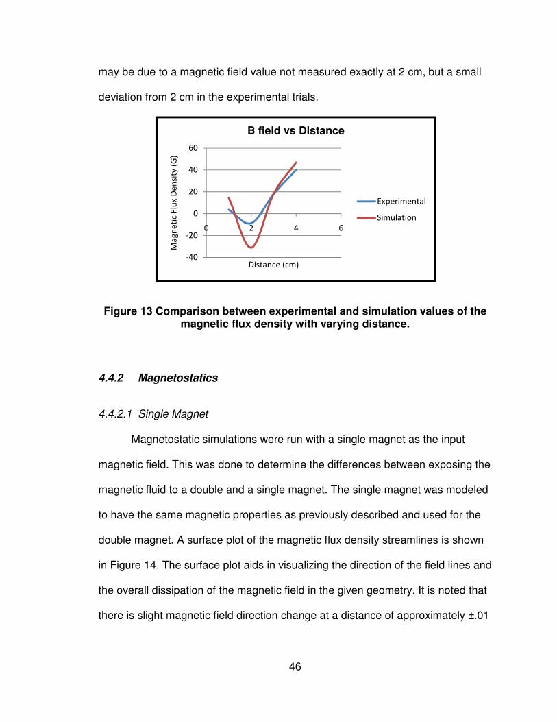
has a sinusoidal profile. This profile represents the pulsatile motion experienced

by the blood from the pumping of the heart. Equation 18 was used as the inlet

boundary condition [72].

(17)

where, U0 is the input velocity magnitude, ω is the frequency in radians and t is

the time in seconds. The addition of the squared square root sinusoidal wave

term eliminates negative values, and thus better represents the motion created

by the pumping of the heart.

During the time dependent model, the input velocity U0, the mass fraction,

the relative permeability and the strength of the permanent magnets are varied

as described in section 4.3 and 4.3.1.

This model initially solves a parametric problem, by slowly increasing the

input velocity U0 from 0 m/s to 0.5 m/s. It then solves the laminar flow model, by

using the BDF solver with two degrees for the time dependency and the

PARADISO solver for the nonlinearities associated with the problem. The

PARADISO solver is a fast solver, appropriate for multi-core capabilities.

Following the laminar flow solution, the model uses these solutions as initial

45

values for the velocity and pressure, and simultaneously solves for the magnetic

field and the new velocities and pressure when magnetic interactions are taken

into consideration. During this last step, the solver used for the time dependency

is the generalized alpha with global tolerances of 0.0000000001 and the MUMPS

solver for the nonlinearities in the model.

4.4 Results

The following section describes the results encountered in the finite

element model for the simulations using a dual magnet configuration and a single

magnet. The parametric variations described in the previous section were

implemented, and the corresponding trends were observed. Comparison of the

parallel magnet configuration and of a single magnet was only done for the

profile of the magnetic flux density with varying distance in the magnetostatics,

section 3.3.1. The general correlations for the remainder of the parametric

sweeps were similar and results were only included for the dual parallel magnet

configuration.

4.4.1 Validation

The results from the validation simulation are seen in Figure 13. The

general profile of the results given by the finite element model and the

experimental results are similar. This indicates that the finite element model must

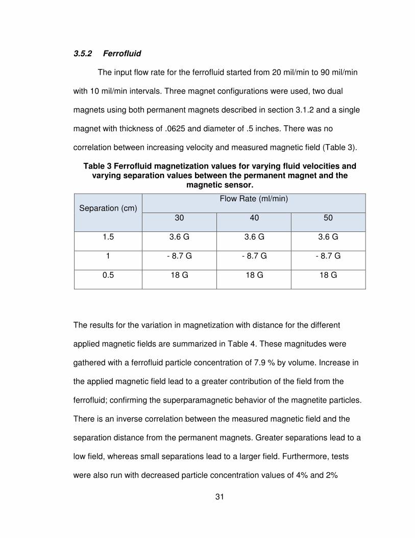
be properly set-up and. The greatest deviations in the results are seen when the

magnetic field lines change in direction at a distance of 2 cm. These differences

46

may be due to a magnetic field value not measured exactly at 2 cm, but a small

deviation from 2 cm in the experimental trials.

Figure 13 Comparison between experimental and simulation values of the magnetic flux density with varying distance.

4.4.2 Magnetostatics

4.4.2.1 Single Magnet

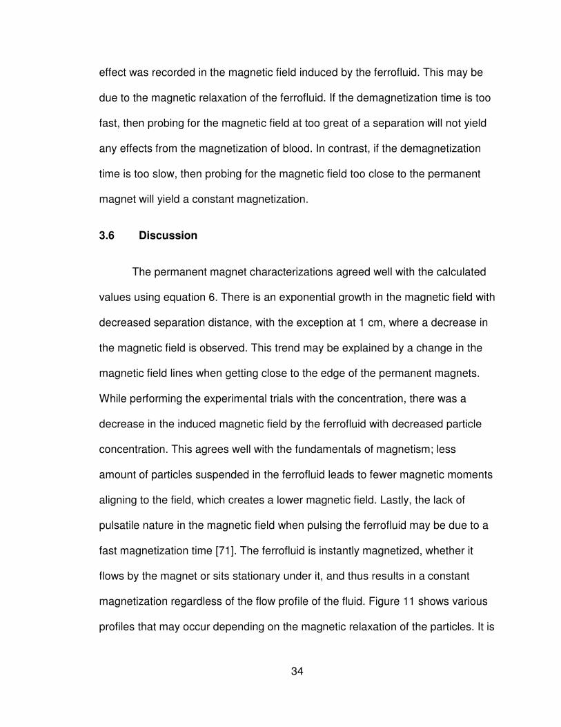
Magnetostatic simulations were run with a single magnet as the input

magnetic field. This was done to determine the differences between exposing the

magnetic fluid to a double and a single magnet. The single magnet was modeled

to have the same magnetic properties as previously described and used for the

double magnet. A surface plot of the magnetic flux density streamlines is shown

in Figure 14. The surface plot aids in visualizing the direction of the field lines and

the overall dissipation of the magnetic field in the given geometry. It is noted that

there is slight magnetic field direction change at a distance of approximately ±.01

-40

-20

0

20

40

60

0 2 4 6

Ma

gn

eti

c F

lux

De

nsi

ty (

G)

Distance (cm)

B field vs Distance

Experimental

Simulation

47

m from the center, when looking at the field on the top boundary of the capillary

glass.

Figure 14 Single magnet magnetic flux density surface plot. Surface indicates the magnetic flux density norm (G), and the contour lines the

magnetic vector potential (Wb/m).

Figure 15 Magnetic flux distance variation with distance for a single magnet along the top boundary of the glass capillary.

0

200

400

600

800

0 0.02 0.04 0.06 0.08 0.1 0.12 0.14Ma

gn

eti

c F

lux

De

nsi

ty (

G)

Distance (m)

Magnetic Flux Density vs Distance

48

Magnetic flux density was tracked along the top boundary of the capillary

tube, to identify the effect of the separation distance from the permanent magnet.

It is observed in Figure 15 that the maximum magnetic flux density reaches a

value of 722.1 G at the center of the magnet. A uniform decay is observed in the

magnetic field as the distance from the permanent magnet is increased. The

magnetization of blood was seen to follow the same shape of the magnetic field

(Figure 16), but with an opposite direction. The opposite shape of the magnetic

flux density contribution from blood represents the behavior of oxygenated blood,

which is diamagnetic in nature. This means its magnetic moments align in the

opposite direction of the applied field, and subtracts from the overall magnetic

flux density. The small dips seen approximately ±.01 m around the center of the

signal are due to the change in the direction of the magnetic field and enhanced

in the magnetization of blood. This dip is not evident in Figure 15 due to the small

nature of the change in the magnetic field, and the large scale of the values

plotted.

Figure 16 Magnetic flux contribution from blood with a single magnet.

-0.000025

-0.00002

-0.000015

-0.00001

-0.000005

0

0 0.02 0.04 0.06 0.08 0.1 0.12 0.14

B B

loo

d (

G)

Distance (m)

Magnetic Flux Density Contribution from Blood

49

4.4.2.2 Double Magnet

The surface plot created in COMSOL, (Figure 17) aids in visualizing the

magnetic fields radiated by the permanent magnets and the magnetization of

blood. In the surface plot, the magnetic flux density magnitude is shown as

varying colors throughout the finite element model, accompanied by the field

streamlines. It is noted that a very uniform field is created between the two

parallel magnets at their center points. The highest magnetic flux density was

observed at the magnet’s edges with a value of 7774 G. The lowest magnetic

flux was seen at the edges of the main domain, with a value of 1.327x10-6 G. Two

symmetrical spots along the centerline between both permanent magnets were

also identified as a low magnitude field in the middle of a high field, with values of

approximately 100G.

Figure 17 Surface plot of the magnetic flux density in the dual magnet configuration. Surface indicates the magnetic flux density norm (G), and

the contour lines the magnetic vector potential (Wb/m).

50

Figure 18 shows a plot of the magnetic flux density with varying distance

from the permanent magnet. The maximum magnetic flux density value is

observed at the center of the magnet with a value of 1211 G. This value is twice

the maximum magnetic flux density observed with a single magnet. A rapid

decay in the magnetic flux is observed from the center of the permanent

magnets. A dip in the magnetic flux is seen at a distance of 1 cm away from the

center of the permanent magnet; this drop corresponds to the spots of low

magnetic flux density seen in the surface plot. This is due to a change in the

magnetic field lines, which corresponds to the changes from the highly uniform

field seen between the magnets and the curved field surrounding the magnets.

Figure 18 Magnetic flux distance variation with distance for dual magnets along the top boundary of the glass capillary.

It was found that the magnetization of the magnetic fluid, in this instance

blood, has a maximum contribution to the magnetic field of 2.06x10-5 G in the

opposite direction (Figure 19). This maximum was observed at the center of the

0

200

400

600

800

1000

1200

1400

0 0.02 0.04 0.06 0.08 0.1 0.12 0.14

Ma

gn

eti

c F

lux

De

nsi

ty N

orm

(G

)

Distance (m)

Magnetic Flux Density vs. Distance

51

permanent magnets, where the highest field concentration occurred. The overall

behavior of the magnetic flux density contribution from the blood with respect to

distance was similar to that of the permanent magnets, but with opposing

direction.

Figure 19 Magnetic flux contribution from blood with a dual magnet.

To verify the relative permeability of the conducting medium, the B-H

curve was reproduced using a 1-D plot in COMSOL (Figure 20). The magnetic

flux density was plotted against the magnetic field; the slope of this line is the

relative permeability of the permanent magnets used. It is observed that the there

is an increase in magnetic flux density with increased magnetic field. This relation

corresponds well with the positive value stated as the relative permeability in air.

Additionally, the line was fitted using linear regression; the resultant is

y = x – 7e-14

(18),

where y represents the magnetic flux density and the magnetic field. The slope of

the fitted equation is 1.0, which is in agreement with the relative permeability of

-0.00003

-0.00002

-0.00001

0

0.00001

0 0.02 0.04 0.06 0.08 0.1 0.12 0.14

B b

loo

d (

G)

Distance (m)

Magnetic Flux Density Contribution from Blood

52

the conducting medium which is air. The y intercept of the equation is -7e-14,

which can be approximated as zero.

Figure 20 Magnetic field variations against the magnetic flux density.

A parametric study was performed by varying the remnant magnetic flux

input value (Figure 21). This corresponds to varying the applied magnetic field

emanating from the permanent magnets. The remnant flux varied from 0 to 2T in

0.1T increments. A linear increase in the magnetic flux density was seen by

increasing the applied field. Accordingly, the blood magnetic flux field contribution

also experienced a linear increase with values varying from zero to a maximum

of 3.21x10-5 G in the opposite direction of the field (Figure 22).

y = x - 7e-14

0

200

400

600

800

1000

1200

1400

0 200 400 600 800 1000 1200 1400Ma

gn

eti

c F

lux

De

nsi

ty (

G)

Magnetic Field (Oe)

BH curve

53

Figure 21 Parametric sweep of remnant magnetic flux densities.

Figure 22 Blood induced magnetic flux density with a remnant magnetic flux.

0

200

400

600

800

1000

1200

1400

1600

1800

2000

0 0.02 0.04 0.06 0.08 0.1 0.12 0.14

Ma

gn

eti

c F

lux

De

nsi

ty (

G)

Distance (m)

Parametric Sweep Remnant Magnetic Flux Density

B rem = 0.0 TB rem = 0.1 TB rem = 0.2 TB rem = 0.3 TB rem = 0.4 TB rem = 0.5 TB rem = 0.6 TB rem = 0.7 TB rem = 0.8 TB rem = 0.9 TB rem = 1.0 TB rem = 1.1 TB rem = 1.2 TB rem = 1.3 TB rem = 1.4 TB rem = 1.5 TB rem = 1.6 TB rem = 1.7 TB rem = 1.8 TB rem = 1.9 T

-0.000035

-0.00003

-0.000025

-0.00002

-0.000015

-0.00001

-0.000005

0

0 5000 10000 15000 20000 25000

B b

loo

d (

G)

Remnant Magnetic Flux (G)

Blood Induced Magnetic Flux Density

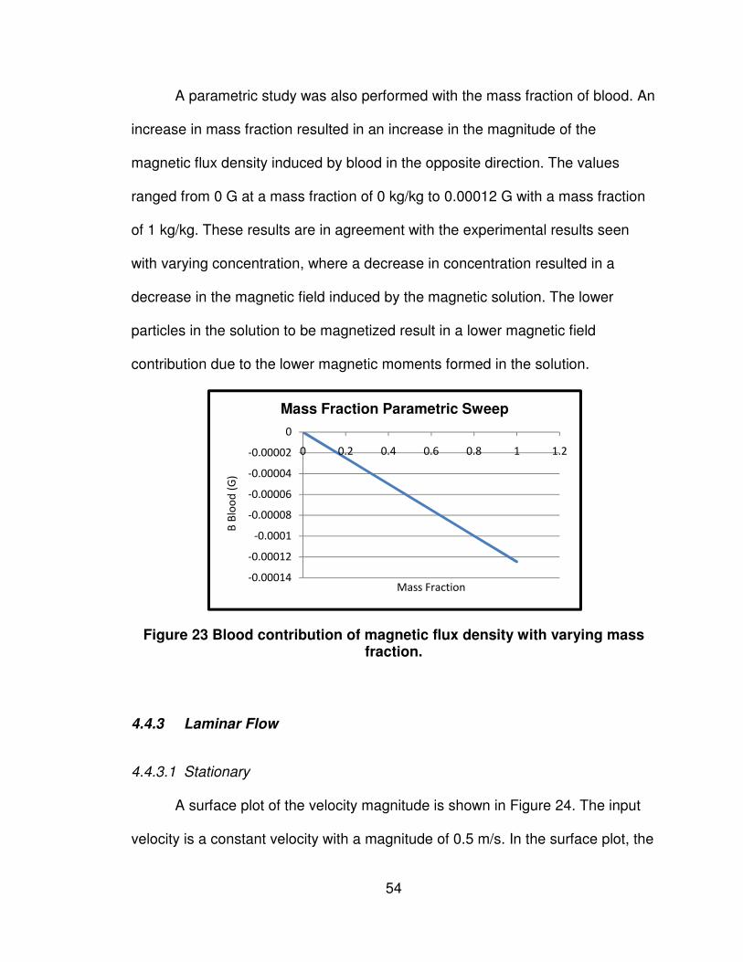
54

A parametric study was also performed with the mass fraction of blood. An

increase in mass fraction resulted in an increase in the magnitude of the

magnetic flux density induced by blood in the opposite direction. The values

ranged from 0 G at a mass fraction of 0 kg/kg to 0.00012 G with a mass fraction

of 1 kg/kg. These results are in agreement with the experimental results seen

with varying concentration, where a decrease in concentration resulted in a

decrease in the magnetic field induced by the magnetic solution. The lower

particles in the solution to be magnetized result in a lower magnetic field

contribution due to the lower magnetic moments formed in the solution.

Figure 23 Blood contribution of magnetic flux density with varying mass fraction.

4.4.3 Laminar Flow

4.4.3.1 Stationary

A surface plot of the velocity magnitude is shown in Figure 24. The input

velocity is a constant velocity with a magnitude of 0.5 m/s. In the surface plot, the

-0.00014

-0.00012

-0.0001

-0.00008

-0.00006

-0.00004

-0.00002

0

0 0.2 0.4 0.6 0.8 1 1.2

B B

loo

d (

G)

Mass Fraction

Mass Fraction Parametric Sweep

55

development of the fluid is seen at the inlet, with a boundary layer at the walls

and the maximum velocity through the centerline of the capillary. The maximum

velocity is 0.753 m/s, due to the development of the fluid. The parabolic nature of

the Poiseuille flow can be seen by the arrow plot shown at the outlet of the

capillary in Figure 25. A parametric study was run, to determine the maximum

flow velocity at various input velocities. The results of the maximum flow

velocities are shown in Figure 26, where the input velocity was varied from 0 m/s

to 0.5 m/s with a step of 0.1 m/s.

Figure 24 Surface plot of constant velocity in capillary glass with an input velocity of .5 m/s.

Figure 25 Poiseuille flow representation by an arrow plot, observed at the

Figure 26 Constant velocity para

4.4.3.2 Transient – Pulsatile Flow

A pulsatile flow was modeled in COMSOL by using equation

input velocity profile. The sinusoidal nature of the fluid profile with respect to time

0

0.1

0.2

0.3

0.4

0.5

0.6

0.7

0.8

0 0.02

Ve

loci

ty (

m/s

)

Constant Input Velocity Parametric Sweep

56

seuille flow representation by an arrow plot, observed at the outlet of the capillary tube.

Constant velocity parametric sweep. Values vary m/s with 0.1 m/s intervals.

Pulsatile Flow

A pulsatile flow was modeled in COMSOL by using equation

The sinusoidal nature of the fluid profile with respect to time

0.02 0.04 0.06 0.08 0.1 0.12Distance (m)

Constant Input Velocity Parametric Sweep

seuille flow representation by an arrow plot, observed at the

from 0 to 0.5

A pulsatile flow was modeled in COMSOL by using equation 18 as the

The sinusoidal nature of the fluid profile with respect to time

V = 0 m/s

V = .1 m/s

V = .2 m/s

V = .3 m/s

V = .4 m/s

V = .5 m/s

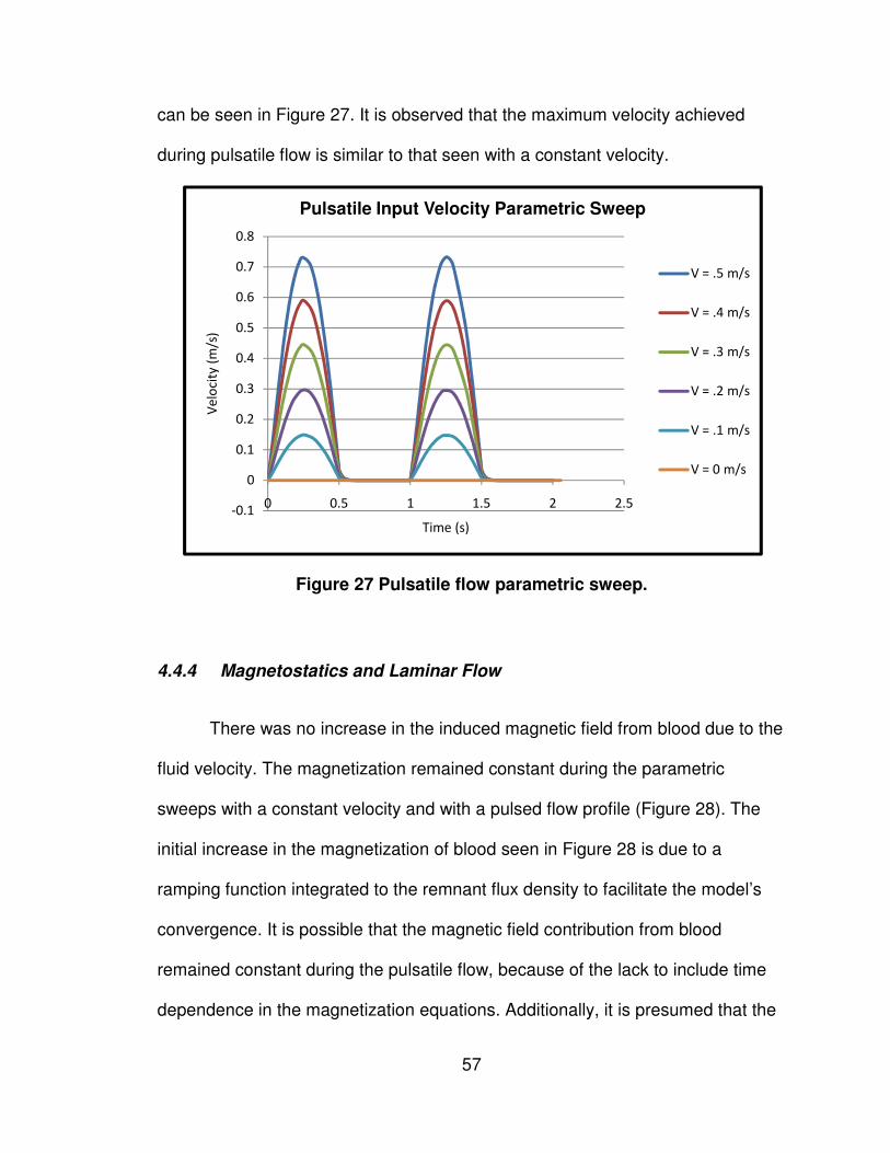
57

can be seen in Figure 27. It is observed that the maximum velocity achieved

during pulsatile flow is similar to that seen with a constant velocity.

Figure 27 Pulsatile flow parametric sweep.

4.4.4 Magnetostatics and Laminar Flow

There was no increase in the induced magnetic field from blood due to the

fluid velocity. The magnetization remained constant during the parametric

sweeps with a constant velocity and with a pulsed flow profile (Figure 28). The

initial increase in the magnetization of blood seen in Figure 28 is due to a

ramping function integrated to the remnant flux density to facilitate the model’s

convergence. It is possible that the magnetic field contribution from blood

remained constant during the pulsatile flow, because of the lack to include time

dependence in the magnetization equations. Additionally, it is presumed that the

-0.1

0

0.1

0.2

0.3

0.4

0.5

0.6

0.7

0.8

0 0.5 1 1.5 2 2.5

Ve

loci

ty (

m/s

)

Time (s)

Pulsatile Input Velocity Parametric Sweep

V = .5 m/s

V = .4 m/s

V = .3 m/s

V = .2 m/s

V = .1 m/s

V = 0 m/s

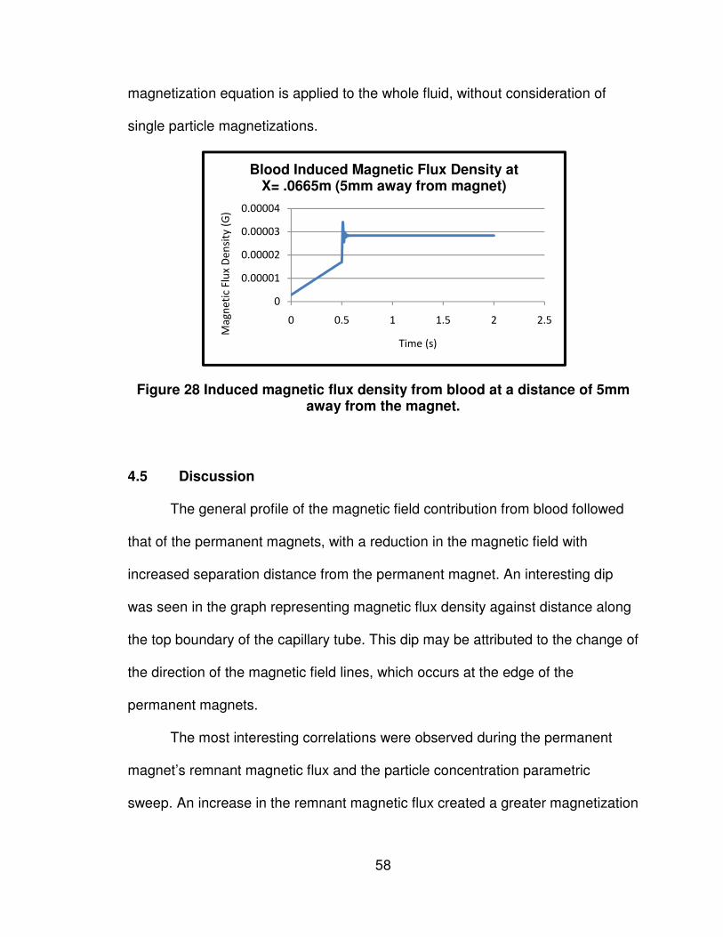
58

magnetization equation is applied to the whole fluid, without consideration of

single particle magnetizations.

Figure 28 Induced magnetic flux density from blood at a distance of 5mm away from the magnet.

4.5 Discussion

The general profile of the magnetic field contribution from blood followed

that of the permanent magnets, with a reduction in the magnetic field with

increased separation distance from the permanent magnet. An interesting dip

was seen in the graph representing magnetic flux density against distance along

the top boundary of the capillary tube. This dip may be attributed to the change of

the direction of the magnetic field lines, which occurs at the edge of the

permanent magnets.

The most interesting correlations were observed during the permanent

magnet’s remnant magnetic flux and the particle concentration parametric

sweep. An increase in the remnant magnetic flux created a greater magnetization

0

0.00001

0.00002

0.00003

0.00004

0 0.5 1 1.5 2 2.5

Ma

gn

eti

c F

lux

De

nsi

ty (

G)

Time (s)

Blood Induced Magnetic Flux Density at X= .0665m (5mm away from magnet)

59

in blood and thus there was a greater contribution to the magnetic field from the

blood. During the concentration parametric sweeps, an increase in concentration

created an increase in the magnetic field contributed from blood. This agrees well

with the fundamentals of magnetism, where greater particle concentration means

a greater net magnetic moment alignment from the solution. Small variations of

the magnetic field were seen during the mass fraction parametric sweep. This

indicates that a sensor to detect blood flow using the magnetization of blood will

be less sensitive to iron concentration fluctuations in the blood, due to anemia or

other biological conditions.

The results when coupling the laminar flow and the magnetostatics did

not yield any correlations between the flow velocity and the contribution to the

magnetic field from the blood. Even when pulsing the fluid flow, the

magnetization of the blood remained constant. It is presumed this is due from not

incorporating a time dependency on the magnetization of the blood. The time

dependency would account for the time it takes a particle to magnetize and

demagnetize. This is represented by

(19),

where M is the magnetization perturbation from the equilibrium magnetization M0

(represented by equation 13 & 14), and � is the relaxation time constant. The

relaxation time constant is defined as

60

(20),

where n f is the viscosity of the fluid, Vh is the volume occupied by the magnetic

particles, m is the magnetic moment of the magnetic particles and H is the

applied magnetic field. For blood, the typical relaxation time constant is in the

order of seconds [67].

Equation 19 may represent an important factor in order to see a varying

disturbance in the magnetic field; it is thought that by using a magnetization

equation which is not time-dependent, it is assumed that the fluid has achieved

an equilibrium magnetization, and will remain constant. Carefully examining

equations 13 & 14, which was used in the simulations, it is noted that the

resultant calculated magnetization value is only dependent in space. Thus, with a

defined fluid magnetic susceptibility and a vector potential that varies in space, a

magnetization is calculated at a given point. The calculated magnetization for the

fluid domain will be the same at a specific coordinate, regardless of time and

velocity variations. It is probable that equations 13 & 14 do not incorporate

particle velocity variations, but simply considers the entire fluid as a whole

substance. In contrast, equation 19 incorporates the effect of magnetizing a

single particle, the time it takes for it to magnetize and demagnetize and

accounts for the influence in the velocity field on the single fluid particle. The

nature of the phenomenon seen by Phua et al. [1] is described in detail by Axel

when explaining the fundamentals of blood flow effects in magnetic resonance

imaging. Suryan et al. observed that a magnetic fluid that flowed through a coil

61

initially had an increased signal and it decreased with the increase of velocity

[75]. During slow flow “the new spins were strongly magnetized and gave a

strong signal, whereas with rapid flow, the upstream fluid was less completely

magnetized due to less time spent in the magnet and gave a weaker signal” [76].

This effect is only seen if the saturation magnetization of the fluid has not been

achieved with the applied magnetic field. If a paramagnetic fluid with Poiseuille

flow is considered, flowing through a tube as shown in Figure 29, the

magnetization effect with respect to time seen during the solution’s flow is

represented by a nonlinear decay as seen in Figure 30. The time it takes to reach

no magnetization change is represented by the length of the magnetized fluid

over the mean velocity of the fluid.

Figure 29 Magnetized particle movement representation of length L in a tube with mean velocity V and Poiseuille flow [76].

62

Figure 30 Magnetization distribution with time for particles in Poiseuille flow [76].

In the case of blood particles with pulsatile flow, the magnetization of the

fluid will yield a dip in the net magnetic field of the permanent magnet. The

distribution of the magnetization of blood with respect to the distance traveled in

one heartbeat, with an input velocity of 0.5 m/s, may be represented with Figure

31. The largest magnitude in magnetization is achieved when the flow dwells

underneath the magnet. The effects of magnetization and demagnetization can

be represented by the time dependent magnetization decay curve. Thus, blood

magnetization is seen as increasing dips in the magnetic field while approaching

the permanent magnet and demagnetization as decreasing dips while flowing

away from the magnet.

63

Figure 31 Magnetization of blood during one heartbeat.

V

64

Chapter 5 – Conclusion and Future Work

The objective of this thesis was to acquire in-depth understanding of the

phenomenon encountered by Phua et al. [1]. It was not possible to replicate this

study neither experimentally nor analytically. During experimentation, it was

difficult to acquire a commercially available sensor that could measure the

magnetic disturbances created by the pulsatile motion of the blood. Moreover,

blood’s sensitivity was found to be in the order of 10-5, which meant that in order

to acquire this signal, custom magnetic shielding and amplification circuitry

needed to be implemented. Furthermore, the magnetic interference of electronics

generated by equipment in laboratories creates a lot of noise in the signal.

An analytical model using COMSOL Multiphysics with the equations

simulating the behavior of blood in an applied magnetic field was also created.

Despite various simulations and attempts in changing the geometry, magnetic

properties, addition of electrical properties and using fine meshes and high

tolerances, the fluctuations in the magnetic field due to blood’s pulsatile motion

were not seen. The magnetization equation used in the model, was only

dependent on space, lacking the variations seen during the time dependent

pulsatile motion of blood. On further investigation, a time dependent

magnetization equation was found. This is thought to be the missing link in the

finite element model which accounts for particle magnetization relaxation, and

65

the velocities of the fluid, and will allow for the visualization of the fluctuations in

the magnetic field due to blood.

At this point it is beneficial to understand the physical behavior behind

disturbances in the magnetic field created by the pulsatile motion of blood. The

most important factor which could be attributed to this phenomenon is the

exposure time. Blood which dwells under the permanent magnet for a longer

time, gets magnetized to a higher degree, and exhibits a greater magnetic

moment alignment. During fast flow, the blood is exposed to the magnetic field

for less time and thus has a much smaller magnetization. Therefore, one would

expect a valley to occur during the lower duration diastolic phase and minimal

magnetization during the longer systolic phase. This theory has been previously

formulated in studies to acquire blood flow during magnetic resonance imaging,

and experimentally proven [75]. A secondary effect, also as important in the

successful acquisition of the disturbance signal, is the relaxation time. If the

relaxation of a magnetic solution is too fast, than the magnetic solution will lose

its magnetization before it reaches the magnetic sensor and no magnetic

disturbance will be measured. Moreover, if the magnetic solution is instantly

magnetized, the magnetic fluid will appear to always be evenly magnetized

regardless of the pulsed nature of the flow. Blood has a magnetic relaxation in

the order of a second, which is important in the successful acquisition of the

disturbance signal when the frequency of the pulsing fluid is 1 Hz.

This thesis has demonstrated that the use of a magnetic sensor to non-

invasively measure blood flow is technically challenging due to the following:

66

• The magnitude of blood’s contribution to a magnetic field of 1200G is in

the order of ~10-5 G, which is much smaller than earth’s magnetic field

(~.3 G) and the magnetic signatures of many electronics in the

environment.

• Blood’s magnetic field contribution can be increased by using larger

applied fields; this is limited by the magnetic sensor and its ability to

maintain the sensitivity needed during larger measurement ranges.

• Magnetic solutions with higher magnetic susceptibilities cannot be used,

since their magnetic properties, such as the magnetization relaxation,

does not match that of blood.

Future work for this project includes the creation or acquisition of a

magnetic sensor with high sensitivities, in order to measure the magnetic

disturbances created by blood. If this is accomplished, it is desired to use blood

in further in vitro experimentation, and perhaps determine the effect of static and

alternating magnetic fields of varying magnitudes. In the finite element model, it

is desired to implement the time dependent magnetization, which should lead to

the successful replication of the MMSB phenomenon. Furthermore, it is desired

to assess the applied field created by varying permanent magnet geometries and

configurations, such as solenoids, shifted dual magnets and large single

magnets.

67

References

[1] Phua, C. T., Lissorgues, G., and Mercier, B., 2009, "Non-Invasive Acquisition of Blood Pulse using Magnetic Disturbance Technique," International Conference of Biomedical Engineering (ICBME), pp. 786-789. [2] Cherniak, R. M., 1983, "Pulmonary Function Testing," Paschalides Publications, pp. 274-276. [3] Frattola, A., 1993, "Prognostic Value of 24-Hour Blood Pressure Variability," Journal of Hypertension.Supplement, 11(10) pp. 1133. [4] Bonnet, M. H., 1998, "Heart Rate Variability in Insomniacs and Matched Normal Sleepers," Psychosomatic Medicine, 60(5) pp. 610. [5] Kanakis, G., Kesisoglou, I., Mpothnavas, A., 1992, "Computers in the Field of Medicine," Health Gazette, 3(4) pp. 48-50. [6] S.M. Burns, 2006, "AACN protocols for practice: noninvasive monitoring," Jones and Bartlett Publishers, . [7] Pinsky, M., and Payen, D., 2005, "Functional Hemodynamic Monitoring." Critical Care, 9(6) pp. 566-572. [8] Gianoulis, N., and Liarmakopoulos, I., 1997, "Invasive Measurement of Blood Pressure," Nosileftiki 1, pp. 40-44. [9] Petrie, J. C., 1986, "Recommendations on Blood Pressure Measurement." British Medical Journal (Clinical Research Ed.1981), 293(6547) pp. 611. [10] Kotrotsiou, E., Tsikragoulas, P., and Ioannidou, C., 2002, "Principles of Hemodynamic Monitoring," ICUs and Nursing Journal, (10) . [11] Weisel, R. D., 1975, "Measurement of Cardiac Output by Thermodilution," The New England Journal of Medicine, 292(13) pp. 682. [12] Kerola, J., 2002, "Non-Invasive Blood Pressure Data Acquisition Employing Pulse Transit Time Detection," Engineering in Medicine and Biology Society, 1996.Bridging Disciplines for Biomedicine.Proceedings of the 18th Annual International Conference of the IEEE, 3pp. 1308.

68

[13] Jacobs, J. L., Embree, P., Glei, M., 2004, "Characterization of a novel heart and respiratory rate sensor," Engineering in Medicine and Biology Society, 2004. IEMBS '04. 26th Annual International Conference of the IEEE, Anonymous 1, pp. 2223-2226. [14] Torres-Pereira, L., Ruivo, P., Torres-Pereira, C., 1997, "A noninvasive telemetric heart rate monitoring system based on phonocardiography," Industrial Electronics, 1997. ISIE '97., Proceedings of the IEEE International Symposium on, Anonymous pp. 856-859 vol.3. [15] Mermel, L. A., McCormick, R. D., Springman, S. R., 1991, "The Pathogenesis and Epidemiology of Catheter-Related Infection with Pulmonary Artery Swan-Ganz Catheters: A Prospective Study Utilizing Molecular Subtyping," The American Journal of Medicine, 91(3, Supplement 2) pp. S197-S205. [16] Vogel, R., Lefree, M., Bates, E., 1984, "Application of Digital Techniques to Selective Coronary Arteriography: Use of Myocardial Contrast Appearance Time to Measure Coronary Flow Reserve," American Heart Journal, pp. 107-153. [17] Marcus, M. L., 1987, "Methods of Measurement of Myocardial Blood Flow in Patients: A Critical Review," Circulation, 76(2) pp. 245. [18] Marcus, M., 1981, "Measurements of Coronary Velocity and Reactive Hyperemia in the Coronary Circulation of Humans," Circulation Research, 49(4) pp. 877. [19] Bowes, W., Corke, B., and Hulka, J., 1989, "Pulse Oximetry: A Review of the Theory, Accuracy, and Clinical Applications.," Obstetrics and Gunecology, 74(3.2) pp. 541-546. [20] Mengelkoch, L., Martin, D., and Lawler, J., 1994, "A Review of the Principles of Pulse Oximetry and Accuracy of Pulse Oximeter Estimates during Exercise.," Physical Therapy, 74(1) pp. 40-49. [21] Aoyagi, T., 2007, "Multiwavelength Pulse Oximetry: Theory for the Future," Anesthesia and Analgesia, 105(6S Suppl) pp. S53. [22] Ericson, M. N., 2002, "In Vivo Application of a Minimally Invasive Oximetry Based Perfusion Sensor," Proceedings of the Annual International Conference of the IEEE Engineering in Medicine and Biology Society, 3pp. 1789. [23] Dung Nguyen, Yamada, S., Byung-Kwon Park, 2007, "Noise Considerations for Remote Detection of Life Signs with Microwave Doppler Radar," Engineering in Medicine and Biology Society, 2007. EMBS 2007. 29th Annual International Conference of the IEEE, pp. 1667-1670.

69

[24] Amit, G., Gavriely, N., Lessick, J., 2005, "Automatic extraction of physiological features from vibro-acoustic heart signals: correlation with echo-doppler," Computers in Cardiology, 2005, Anonymous pp. 299-302. [25] Tropea, C., 1995, "Laser Doppler Anemometry: Recent Developments and Future Challenges," Measurement Science Technology, 6pp. 605. [26] Vennemann, P., 2007, "In Vivo Whole-Field Blood Velocity Measurement Techniques," Experiments in Fluids, 42(4) pp. 495. [27] Van De Water, J. M., 2003, "Impedance Cardiography*," Chest, 123(6) pp. 2028. [28] Hung, J., Lang, R., Flachskampf, F., 2007, "3D Echocardiography: A Review of the Current Status and Future Directions," Journal of the American Society of Echocardiography, (20) pp. 213-233. [29] Brooks, R. A., 1976, "Principles of Computer Assisted Tomography (CAT) in Radiographic and Radioisotopic Imaging," Physics in Medicine and Biology, 21pp. 689. [30] Malmivuo, J., and Plonsey, R., 1995, "Bioelectromagnetism - Principles and Applications of Bioelectric and Biomagnetic Fields," . [31] Kanai, H., Yamano, E., Nakayama, K., 1974, "Transcutaneous Blood Flow Measurement by Electromagnetic Induction," Biomedical Engineering, IEEE Transactions on, BME-21(2) pp. 144-151. [32] Fegler, G., 1954, "Measurement of Cardiac Output in Anaesthetized Animals by a Thermo-Dilution Method," Experimental Physiology, 39(3) pp. 153. [33] Swan, H. J. C., 1970, "Catheterization of the Heart in Man with use of a Flow-Directed Balloon-Tipped Catheter," The New England Journal of Medicine, 283(9) pp. 447. [34] Connors, A. F., 1996, "The Effectiveness of Right Heart Catheterization in the Initial Care of Critically III Patients," JAMA (Chicago, Ill.), 276(11) pp. 889. [35] Sandham, J. D., 2003, "A Randomized, Controlled Trial of the use of Pulmonary-Artery Catheters in High-Risk Surgical Patients," The New England Journal of Medicine, 348(1) pp. 5. [36] Hodgson, J. M., LeGrand, V., Bates, E. R., 1985, "Validation in Dogs of a Rapid Digital Angiographic Technique to Measure Relative Coronary Blood Flow during Routine Cardiac Catheterization," The American Journal of Cardiology, 55(1) pp. 188-193.

70

[37] Cusma, J. T., 1987, "Digital Subtraction Angiographic Imaging of Coronary Flow Reserve," Circulation, 75(2) pp. 461. [38] Mancini, G., and Higgins, C., 1985, "Digital Subtraction Angiography: A Review of Cardiac Applications," Progress in Cardiovascular Disease, 18pp. 111. [39] Vatner, S. F., 1970, "Simultaneous Comparison and Calibration of the Doppler and Electromagnetic Flowmeters," Journal of Applied Physiology, 29(6) pp. 907. [40] Wilson, R. F., 1985, "Transluminal, Subselective Measurement of Coronary Artery Blood Flow Velocity and Vasodilator Reserve in Man," Circulation, 72(1) pp. 82. [41] Wilson, R. F., 1986, "Intracoronary Papaverine: An Ideal Coronary Vasodilator for Studies of the Coronary Circulation in Conscious Humans," Circulation, 73(3) pp. 444. [42] Kisslo, J. L., and Adams, D. B., 2000, "Principles of Echocardiography," 2010(06/21) pp. 25. [43] Yancy, C., 2003, "Noninvasive Hemodynamic Monitoring in Heart Failure: Utilization of Impedance Cardiography," Congestive Heart Failure, 9(5) pp. 241. [44] Nieman, K., 2003, "Evaluation of Patients After Coronary Artery Bypass Surgery: CT Angiographic Assessment of Grafts and Coronary Arteries1," Radiology, 229(3) pp. 749. [45] Rich, S., Chomka, E. V., Stagl, R., 1986, "Determination of Left Ventricular Ejection Fraction using Ultrafast Computed Tomography," American Heart Journal, 112(2) pp. 392-396. [46] Reiter, S. J., 1986, "Precision of Measurements of Right and Left Ventricular Volume by Cine Computed Tomography," Circulation, 74(4) pp. 890. [47] Goldstein, J. A., Schiller, N. B., Lipton, M. J., 1986, "Evaluation of Left Ventricular Thrombi by Contrast-Enhanced Computed Tomography and Two-Dimensional Echocardiography," The American Journal of Cardiology, 57(10) pp. 757-760. [48] Wolfkiel, C. J., 1987, "Measurement of Myocardial Blood Flow by Ultrafast Computed Tomography," Circulation, 76(6) pp. 1262. [49] Lee, T. Y., 2002, "Functional CT: Physiological Models," Trends in Biotechnology, 20(8) pp. 3.

71

[50] Schoder, H., 1999, "Blood Flow-Metabolism Imaging with Positron Emission Tomography in Patients with Diabetes Mellitus for the Assessment of Reversible Left Ventricular Contractile Dysfunction," Journal of the American College of Cardiology, 33(5) pp. 1328. [51] Ching, A., and Au-Yong, T., 2004, "Combined Positron-Emission Tomography-Computed Tomography: Merging Form with Function," Journal of Hong Kong College of Radiologists, (7) pp. 102-111. [52] Frydman, L., 2003, "Principles and Features of Single-Scan Two-Dimensional NMR Spectroscopy," Journal of the American Chemical Society, 125(30) pp. 9204. [53] Peller, M., 2003, "Hyperthermia Induces T1 Relaxation and Blood Flow Changes in Tumors. A MRI Thermometry Study in Vivo* 1," Magnetic Resonance Imaging, 21(5) pp. 545. [54] Koskenvuo, J. W., 2001, "Assessing Coronary Sinus Blood Flow in Patients with Coronary Artery Disease: A Comparison of Phase-Contrast MR Imaging with Positron Emission Tomography," AJR, American Journal of Roentgenology, 177(5) pp. 1161. [55] Hough, R.H., and Boehm, W.M., 1913, "Elementary principles of electricity and magnetism, for students in engineering," The Macmillan Company, Newy York, London, . [56] Molinton, A., 2007, "Basic Electromagnetism and Materials," Springer Science, . [57] Reyes, O. V., 2009, "Numerical Simulation and Development of a Ferrofluid Pumping Device Driven by Electromagnets," . [58] Herbert, P., 1976, "Introductory Electromagnetics," John Wiley & Sons, Inc. [59] Griffiths, D.J., 1999, "Introduction to Electrodynamics," Prentice-Hall, Upper Saddle river, New Jersey, . [60] Anonymous 2005, "Magnetism Fundamentals," Springer Science, Boston, . [61] Callister, W.D., 1997, "Magnetic Properties,". [62] Neuringer, J. L., 1964, "Ferrohydrodynamics," The Physics of Fluids, 7pp. 1927. [63] Ramsay, W. N. M., 1957, "The Determination of Iron in Blood Plasma Or Serum," Clinica Chimica Acta, 2(3) pp. 214-220.

72

[64] Khanafer, K. M., 2006, "Modeling Pulsatile Flow in Aortic Aneurysms: Effect of Non-Newtonian Properties of Blood," Biorheology, 43(5) pp. 661. [65] Motta, M., 1998, "High Magnetic Field Effects on Human Deoxygenated Hemoglobin Light Absorption," Bioelectrochemistry and Bioenergetics, 47(2) pp. 297. [66] Tzirtzilakis, E. E., 2005, "A Mathematical Model for Blood Flow in Magnetic Field," Physics of Fluids, 17pp. 077103. [67] Higashi, T., 1993, "Orientation of Erythrocytes in a Strong Static Magnetic Field," Blood, 82(4) pp. 1328. [68] Pai, V. M., Haik, Y., and Chen, C. J., 1996, "Bio-Magnetic Fluid Dynamics," ASME Publication, 237pp. 761-774. [69] Popović, R. S., 1989, "Hall-Effect Devices," Sensors and Actuators, 17(1-2) pp. 39-53. [70] Hansen, V. W., 2002, "RF Exposure of Biological Systems in Radial Waveguides," IEEE Transactions on Electromagnetic Compatibility, 41(4) pp. 487. [71] Payet, B., Donatini, F., and Noyel, G., 1999, "Longitudinal Magneto-Optical Study of Brown Relaxation in Ferrofluids:: Dynamic and Transient Methods. Application," Journal of Magnetism and Magnetic Materials, 201(1-3) pp. 207-210. [72] Phua, C. t., and Lissorgues, G., 2009, "Modeling of Pulsatile Blood Flow in a Weak Magnetic Field," World Academy of Science, Engineering and Technology, (54) pp. 73-76. [73] Taylor, C. A., 1998, "Finite Element Modeling of Blood Flow in Arteries," Computer Methods in Applied Mechanics and Engineering, 158(1-2) pp. 155. [74] Oldenburg, C. M., 2000, "Numerical Simulation of Ferrofluid Flow for Subsurface Environmental Engineering Applications," Transport in Porous Media, 38(3) pp. 319. [75] Suryan, G., 1951, "Nuclear Resonance in Flowing Liquids," Proceedings Mathematical Sciences, 33(2) pp. 107-111. [76] Axel, L., 1984, "Blood Flow Effects in Magnetic Resonance Imaging," AJR, American Journal of Roentgenology, 143(6) pp. 1157.

Documents

Understanding the Interaction Between Blood Flow and an