Understanding the interest-rate growth differential: its importance in long-term debt projections and for policy

David Turner, OECD

UN DESA Expert Group Meeting on the World Economy, LINK Project

October 24-26, 2011, New York

In long-term, fiscal problems not confined to euro area !

0

50

100

150

200

250

300

1990 1992 1994 1996 1998 2000 2002 2004 2006 2008 2010 2012 2014 2016 2018 2020 2022 2024 2026

Gross government debt projections under a stylised  and gradual fiscal consolidation rule

(% of GDP)

USA Japan Euro area

Δd = ‐pb + (r‐g) d‐1 (+sf)

where    d = debt‐to‐GDP ratiopb = primary balance ratior  = effective interest rate on net debtg = nominal  GDP growthsf = stock‐flow adjustment

Source: OECD Economic Outlook, May 2011, chapter 4.

It matters a lot in the long-term : Small changes in (r-g) have large effects on debt projections

0

20

40

60

80

100

120

140

1990

1993

1996

1999

2002

2005

2008

2011

2014

2017

2020

2023

2026

2029

2032

2035

2038

2041

2044

2047

2050

2053

2056

2059

US gross government debt projections under differnt assumptions about (r‐g) differential

Baseline

(r‐g) less 1% pt

(r‐g) less 2% pt

N.B. Likely to understate differences if additional effect from lower fiscal risk premia.

Pre-crisis (r-g) differential in 2000s was much lower than over 1980s and 1990s. Where next ?

‐3.0

‐2.0

‐1.0

0.0

1.0

2.0

3.0

4.0

5.0

6.0

7.0

1981

1982

1983

1984

1985

1986

1987

1988

1989

1990

1991

1992

1993

1994

1995

1996

1997

1998

1999

2000

2001

2002

2003

2004

2005

2006

2007

2008

2009

2010

Interest rate ‐ growth differential for 23 OECD countries

Median

Lower quartile

Upper quartile

The 23 OECD countries have been chosen for consistent time series estimates for potential output and long-term interest rates on 10-year government bonds from 1983. Using nominal potential growth instead of actual GDP growth abstracts from the cycle and so gives a better impression of trend movements.

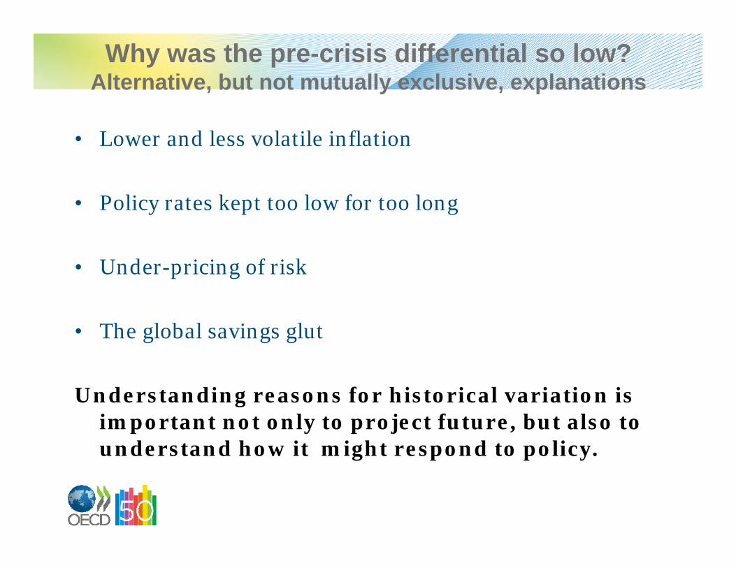
Why was the pre-crisis differential so low? Alternative, but not mutually exclusive, explanations

• Lower and less volatile inflation

• Policy rates kept too low for too long

• Under-pricing of risk

• The global savings glut

Understanding reasons for historical variation is important not only to project future, but also to understand how it might respond to policy.

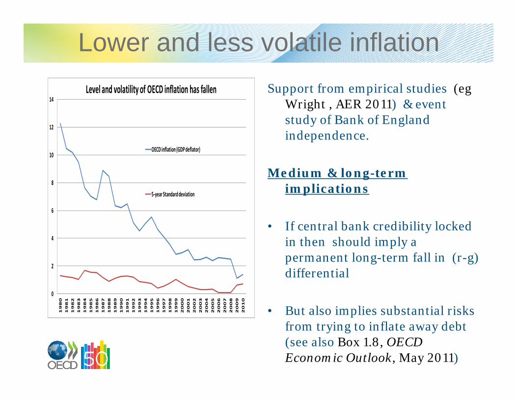
Lower and less volatile inflationSupport from empirical studies (eg

Wright , AER 2011) & event study of Bank of England independence.

Medium & long-term implications

• If central bank credibility locked in then should imply a permanent long-term fall in (r-g) differential

• But also implies substantial risks from trying to inflate away debt (see also Box 1.8, OECD Economic Outlook, May 2011)

0

2

4

6

8

10

12

14

1980

1981

1982

1983

1984

1985

1986

1987

1988

1989

1990

1991

1992

1993

1994

1995

1996

1997

1998

1999

2000

2001

2002

2003

2004

2005

2006

2007

2008

2009

2010

Level and volatility of OECD inflation has fallen

OECD inflation (GDP deflator)

5‐year Standard deviation

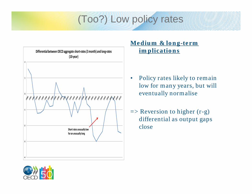
(Too?) Low policy rates

Medium & long-term implications

• Policy rates likely to remain low for many years, but will eventually normalise

=> Reversion to higher (r-g) differential as output gaps close

‐4

‐3

‐2

‐1

0

1

2

Differential between OECD aggregate short‐rates (3 month) and long‐rates (10‐year)

Short rates unusually low for an unusually long 

Risk aversion has increased

Medium & long-term implications

• Financial crisis and new capital requirements have increased risk aversion

• Clear illustration for euro area countries currently under pressure

• Financial markets more discriminating about sovereign debt risk. How much time do USA and Japan have?

‐6.0

‐4.0

‐2.0

0.0

2.0

4.0

6.0

8.0

GRC IRL ITA PRT ESP

(r‐g) differential for euro countries under financial  pressure

Average1980‐95

Average 2000‐07

2010

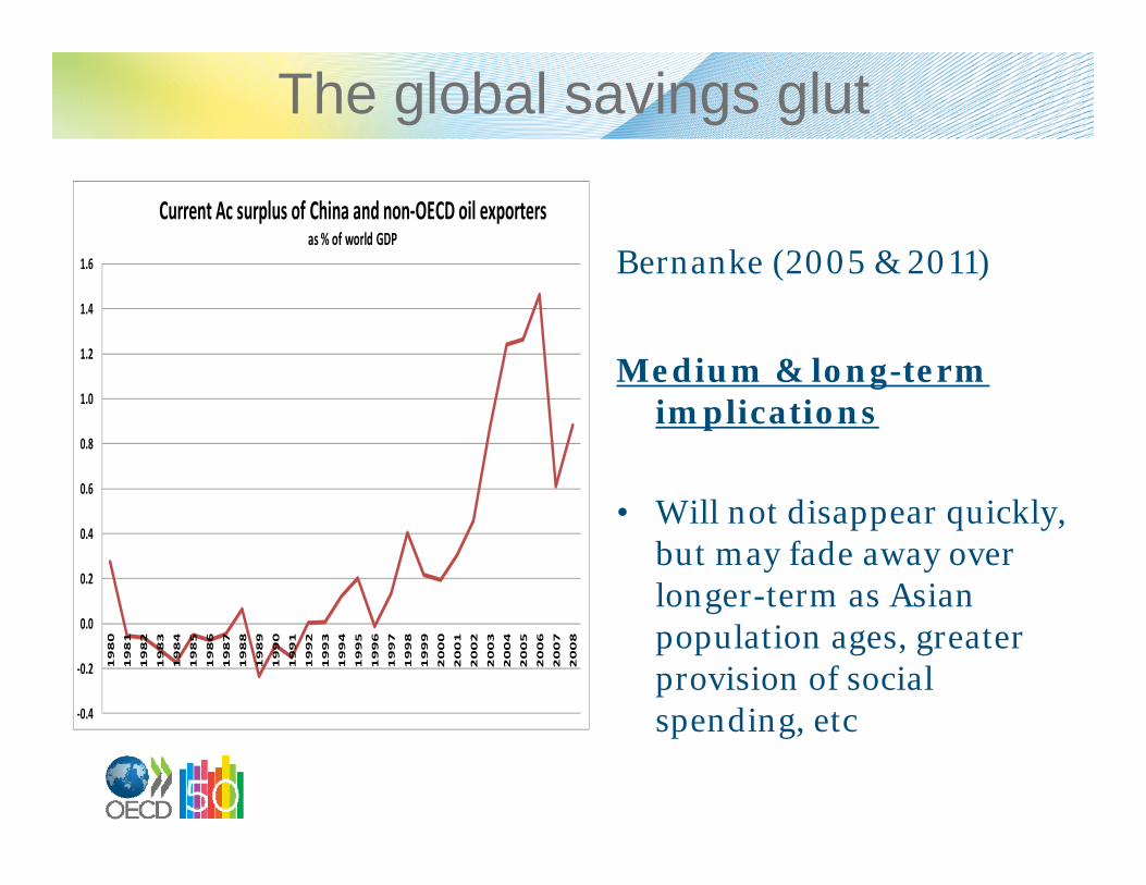
The global savings glut

Bernanke (2005 & 2011)

Medium & long-term implications

• Will not disappear quickly, but may fade away over longer-term as Asian population ages, greater provision of social spending, etc‐0.4

‐0.2

0.0

0.2

0.4

0.6

0.8

1.0

1.2

1.4

1.6

1980

1981

1982

1983

1984

1985

1986

1987

1988

1989

1990

1991

1992

1993

1994

1995

1996

1997

1998

1999

2000

2001

2002

2003

2004

2005

2006

2007

2008

Current Ac surplus of China and non‐OECD oil exportersas % of world GDP

Some simple econometrics to try to discriminate between explanations

• Panel regression, G7 countries, 1980-2010, country fixed effects, Dependent variable (r- g) where r is 10-year govt bond rate and g is growth rate of nominal potential GDP

• All effects statistically significant and correctly signed.

Variable Coefficient t-ratio Long-run

Inflation variability (5 year standard deviation of inflation)

0.29 2.4 0.74

Slope Yield curve(-1)(short minus long rates)

0.25 4.2 0.64

Lagged dependent variable

0.61 10.9 -

..and some support for global savings glut

• Panel regression, G7 countries, 1980-2010, country fixed effects, Dependent variable (r- g) where r is 10-year govt bond rate and g is growth rate of nominal potential GDP.Variable Coeff. t-ratio Long-run

Inflation variability (5 year standard deviation of inflation)

0.19 1.9 0.40

Slope Yield curve(-1)(short minus long rates)

0.31 3.6 0.66

Lagged dependent variable 0.53 8.6 -

Current Ac surplus, China + non-OECD oil exporters (as % world GDP)

-0.77 -2.7 1.64

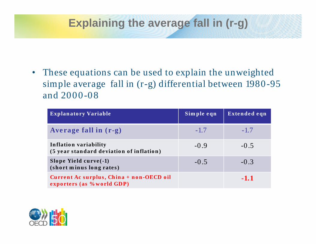
Explaining the average fall in (r-g)

• These equations can be used to explain the unweighted simple average fall in (r-g) differential between 1980-95 and 2000-08

Explanatory Variable Simple eqn Extended eqn

Average fall in (r-g) -1.7 -1.7

Inflation variability (5 year standard deviation of inflation)

-0.9 -0.5

Slope Yield curve(-1)(short minus long rates)

-0.5 -0.3

Current Ac surplus, China + non-OECD oil exporters (as % world GDP)

-1.1

Conclusions (1)

• As policy rates normalise and quantitative easing ends, likely (r-g) will rise as output gaps close.

• Lower and less volatile inflation in 2000s reduced (r-g) by more than 2% pts relative to 1980s & 90s, should be permanent if central banks remain credible, …

• … but this implies risk of substantial cost from trying to inflate debt problems away.

Conclusions (2)• Also some evidence that a part of fall in (r-g) in

2000s is unexplained & so could reappear.

• Experience from euro area that financial markets are now more discriminating about risk.

• Over long-term, countries that are vulnerable include USA and Japan, especially because neither yet has a credible medium-term plan to reduce debt

• To extent that global savings glut is a factor need a global model capable of projecting long-term global savings & investment balances …. Watch this space!

Understanding the interest-rate growth differential: its importance in long-term debt projections and for policy

David Turner, OECD

UN DESA Expert Group Meeting on the World Economy, LINK Project

October 24-26, 2011, New York