Understanding the KST and Asset Allocation - Pring … · Introduction his booklet has been provided with your ... tion within the business cycle and its importance for ... Understanding

1

Understanding the KST

and

Asset Allocation

2

Understanding the KST and Asset Allocation

3

Table of Contents

Introduction .......................................................... 5

Chapter 1: The KST System ................................. 7THE MARKET CYCLE MODEL............................. 11

Chapter 2: Business Cycle Analysis .................... 15THE BOND BAROMETER..................................... 19THE STOCK BAROMETER .................................... 20THE RULE OF 12 .............................................. 21THE INFLATION BAROMETER .............................. 23INFLATION VS. DEFLATION .................................. 23

To order, please call 1.800.221.7514 or 941.364.5850.You can also FAX your order to 941.364.9463 or e-mail yourname and complete shipping address, a credit card numberand expiration date along with a daytime telephone numberto [email protected] and we’ll ship out your order within 48hours of card approval!

For further information on these and other products, pleasevisit our web site at http://www.pring.com.

4


5

Introduction

his booklet has been provided with your subscription oremail registration to provide an understanding of the princi-

pal techniques used in the InterMarket Review and WeeklyUpdate Service, but it is also the basis for my analysis. Whenyou grasp the concepts contained in this booklet, you will have agreater understanding of how markets relate to each other withinthe course of a typical business cycle. Having greater confidencein the conclusions and recommendations from your analysis, willbetter position you, both mentally and emotionally, to act.

Unfortunately, the business cycle approach does not seem towork effectively with individual countries other than the U.S.This is probably due to the fact that external factors have a rela-tively smaller influence on the U.S. economy than on othercountries.

This booklet has been divided into two chapters. The firstdescribes the principal technical vehicle used in the InterMarketReview and Weekly Update Services - the KST system. The sec-ond chapter deals with the business cycle approach and endswith a primer on the relationship between inflation and defla-tion within the business cycle and its importance for assetallocation.

For additional information on the concepts in this publica-tion and other educational materials, please visit our web site atwww.pring.com.

T

Good luck, and good charting!

Martin J. Pring

6


7

The KST System

f you are driving a car in astrange city and need to get

directions, it’s easy to stop at agas station and buy a map.Wouldn’t it be great if youcould also buy an investmentmap pinpointing the marketsproximity to major tops andbottoms?

There’s never been such amap available - until now. Myanalytical approach, the KSTMarket Cycle Model, can helpyou by becoming your invest-ment roadmap. The KST(Know Sure Thing) is a princi-pal technique we use in all ouranalysis for identifying short-,intermediate- and long-termmarket trends. Of course, nosystem is perfect (hence itsname) but the KST approachis dependable enough to helpput the odds in your favor.

The calculation of the KSTassumes that prices at any onetime are determined by the in-teraction of a number ofdifferent time cycles. Mostmomentum indicators or oscil-lators are based on a singletime span and reflect only oneof these cycles. It’s as if youwere guarding the door to abuilding. You could easily see

anyone approaching that par-ticular door, but wouldcompletely miss them trying tobreak in from the other en-trances. The KST gets roundthis problem by including fourdifferent rate of change (ROC)time frames in its calculation.Each one is weighted accord-ing to the length of time span.The longer the span, thegreater the weight. Since rawdata can be very jagged andconfusing, the KST is alsosmoothed so it has a deliber-ate ebb and flow.

How does the KST Systemfit into the bull and bear cycle?Well, there are principally threetrends followed by most inves-tors. These are short, lastingabout 2 to 4 weeks, intermedi-ate, which lasts 6 weeks to aslong as 9 months and the long-term, or primary trend, whichencompasses an 11 month to2 year span.

Chart1-1 shows a long-term KST for the CRB SpotRaw Industrial Material Index.The swings in this indicator areslow and deliberate, butchanges in direction are de-signed to signal trend reversalsat a relatively early stage. Buy-

I

8


ing opportunities typically de-velop when the KST is at, orusually below, zero and start-ing to turn up. The movingaverage has a 9-month timespan. It is the crossovers of thisaverage that trigger KST buyand sell signals.

We can sometimes usechanges in the direction of theKST itself. However, in somesituations we find that the KSTreverses direction and thenquickly whipsaws back. In1990, for instance, the KSTstarted to move sideways butalways remained below its av-erage. The moving average

approach filters out a lot ofthese whipsaw signals whileretaining a good sense of tim-ing. Not all whipsaws arefiltered in this way, but mostare. As an example, look atthe 1993 experience. As longas the KST is above its movingaverage and is rising, the trendis considered to be positive.When it’s below its moving av-erage, it’s considered to benegative. Obviously, the fur-ther this indicator moves awayfrom the equilibrium or zerolevel, the greater the odds thetrend will soon reverse. In sucha situation, the trend is still

CRB Spot Raw Material Index and a Long-term KST

Chart 1-1

9

positive, but the indicator is sooverextended that the risksoutweigh the rewards from thepoint of view of making newpurchases, except for the mostnimble of traders.

The KST is a very useful in-dicator but it does suffer fromsome drawbacks. First, thelongest time span used in itsconstruction is 24-months.This makes it suitable for ana-lyzing trends that revolvearound the 4-year businesscycle, discussed in detail laterin this chapter. Most financialmarkets are sensitive to thistime frame most of the time.

However, when primary trendsare truncated due to politicalor other random and unusualfactors, price reversals developa lot faster than is normally thecase. The highly smoothedKST, on the other hand, can-not react so quickly, whichmeans buy and sell signals de-velop well after the fact.

Second, when bull marketsare long and bear markets rela-tively short, the overall pricemovement encompassing twoor more cycles appears on thechart as a linear trend whichhardly undergoes a correction.The Japanese stock market in

Chart 1-2

Nikkei and a Long-term KST

The KST System

10


the 1980’s (shown in Chart 1-2) and the U.S. market in thelate 1980’s to mid-1990’s, of-fer fine examples. Duringlinear trends where there arevery few cyclic rhythms, a mo-mentum indicator such as theKST may give premature sellsignals, while buy signals willbe unduly late.

For this reason, it’s prudentto remember that KST buy andsell signals are just that - theyare buy and sell signals for mo-mentum, not price. Undernormal circumstances, theprice will go with the momen-tum, but there are many

examples where this does nothappen. Consequently, KSTsignals need to be confirmedwith some kind of trend rever-sal signal in the indicator theyare trying to monitor. We typi-cally use a 12-month movingaverage as featured in Chart 1-1 for the CRB Spot RM Index.Alternatively, it is possible tocombine KST signals withtrendline breaks and price pat-tern completions in the priceindex itself.

We also use KST indicatorsfor identifying other types oftrend changes, specificallyshort (2 to 6 weeks) and inter-

Chart 1-3

Nikkei and a Short-term (Daily) KST

11

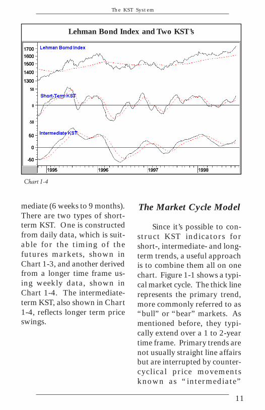
Lehman Bond Index and Two KST’s

Chart 1-4

mediate (6 weeks to 9 months).There are two types of short-term KST. One is constructedfrom daily data, which is suit-able for the timing of thefutures markets, shown inChart 1-3, and another derivedfrom a longer time frame us-ing weekly data, shown inChart 1-4. The intermediate-term KST, also shown in Chart1-4, reflects longer term priceswings.

The Market Cycle Model

Since it’s possible to con-struct KST indicators forshort-, intermediate- and long-term trends, a useful approachis to combine them all on onechart. Figure 1-1 shows a typi-cal market cycle. The thick linerepresents the primary trend,more commonly referred to as“bull” or “bear” markets. Asmentioned before, they typi-cally extend over a 1 to 2-yeartime frame. Primary trends arenot usually straight line affairsbut are interrupted by counter-cyclical price movementsknown as “intermediate”

The KST System

12


trends or “secondary” correc-tions. That’s the thin line inthe figure. These last anywherefrom 6 weeks to many monthsand retrace between 1/3 to 2/3of the previous primary move-ment. Secondary correctionsusually develop because of atemporary change in the per-ceptions of investors towardsthe economic or financialoutlook.

In turn, intermediate trendsare interrupted by even smallerones lasting a couple of weeksor so. These short-term pricemovements are usually causedby random factors which have

little or no bearing on the busi-ness cycle. They are representedin the figure by the dotted line.

From an investment pointof view, the best time to buy iswhen all three trends are bot-toming. Unfortunately, thiscombination is rarely seenbecause the short- and interme-diate-term KST’s usually turnwell ahead of the long-term se-ries. Occasionally, it’s possibleto anticipate a long-term rever-sal. For example, if thelong-term KST starts to flattenout from below zero, theshort- and intermediate-termKST’s trigger a buy signal and

The Four-Year Business Cycle

Figure 1-1

13

the price completes a formation,crosses a moving average, orviolates a moving average. Theimplied reversal in momentumwill usually be strong enoughto allow a reversal in the long-term series. The reverse set ofcircumstances would be true atthe top of a bull market.

This arrangement is alsohelpful once it’s evident thelong-term KST is in a bullishmode vis a vis its moving av-erage, but is not undulyoverextended. This arises fromthe principle that a rising tidelifts all boats. In other words,if the long-term KST is positive

Chart 1-5

Market Cycle Model of the Swiss Franc

Business Cycle Analysis

and not overbought, it’s reason-able to assume the primarytrend is up. Con- sequently,when the short and or the in-termediate series correct andthen reverse direction, this be-comes a signal to buy.

The KST Market CycleModel consists of three oscil-lators that reflect the primary,intermediate- and short-termtime frames as you can see inChart 1-5 featuring the Swissfranc.

The direction of the long-term KST tells us whether theprimary trend is up or downand the level of its maturity.

14


Stock/Bond Ratio and Three KST’s

Chart 1-6

Maximum profit opportunitiesoccur when long-term KST re-verses to the upside from belowzero. When taking short-termpositions, traders should firstconsider the prevailing positionof the long-term KST.

The most important thingto bear in mind is the directionand maturity of the primarytrend. Short and intermediatesignals that are triggered in thesame direction as the maintrend result in the strongest ral-lies, but signals that go againstthe main trend generally givefalse indications.

The KST Market CycleModel can be constructed forany financial market influ-enced by the business cycle andalso is very effective as a toolfor relative strength analysis.Chart 1-6 shows the relativeperformance of stocks againstbonds. These inter-asset rela-tionships can be of invaluablehelp in the asset allocationprocess when combined withthe business cycle barometersdescribed later in this booklet.

15

Figure 2-1

Idealized Business Cycle for the Six Stages of the Business Cycle

Stage I Stage II Stage III Stage IV Stage V Stage VI

Recovery

Recession

BondsStocks

Commodities

CommoditiesStocks

Bonds

¯¯

¯

Chapter 2: Business Cycle Analysis

he 4-year business cyclehas consistently repeated

itself since the beginning of the19th century, when reliable sta-tistics first became available. Atypical cycle averages closer to3.6 years in length and encom-passes an economic expansionand contraction. The contrac-tionary phase normally takesthe form of a decline in the levelof economic activity; i.e., a re-cession, but sometimes islimited to a slowdown in therate of growth, known as agrowth recession.

When an expansion is par-ticularly long, say six to ten

years, it usually includes agrowth recession where theeconomy pauses for breath, butdoesn’t actually contract. Forexample, the recovery that be-gan in 1982 experienced asharp slowdown in growth in1984 and 1985. These“double” cycles are also asso-ciated with two complete“mini” stock and commoditycycles.

This is an important pointbecause the primary trend ofthe financial markets: bonds,stocks, and commodities, aredetermined by the businesscycle.

T

16


Figure 2-1 shows an ideal-ized business cycle. The sinecurve represents the path ofeconomic growth or contrac-tion, while the horizontal lineseparates expansionary periodsfrom those of contraction.History shows an economyundergoes a chronological se-quence of events during acomplete cycle, making it pos-sible to identify turning pointsfor various financial and eco-nomic indicators, as well asbonds, stocks and commodi-ties. Figure 2-1 also showsthese idealized juncture pointsfor the three financial markets.

The six stages of the busi-ness cycle can be identified.Stage 1 occurs when interestrates peak out; i.e., debt pricesturn bullish, but stocks andcommodities are still declining.Stage 2 is signaled when stocksjoin bonds in the bullish campand Stage 3 when all three mar-kets are in uptrends. You canmake more intelligent asset al-location decisions when theprevailing stage of the cycle hasbeen correctly identified. Thechronological sequence hasworked very well (with a fewexceptions) over the last two-hundred-years. However, theleads and lags between these

various events do alter consid-erably from cycle to cycle.Also varying is the magnitudeof price moves by specificmarkets.

We use two techniques toidentify the various stages. Thefirst is a very simple technicalapproach of comparing eachmarket with its 12-month mov-ing average. The proxies weuse are long-term governmentbond prices, the S&P Compos-ite, and the CRB RawIndustrial Commodity Index.We use raw industrial pricesbecause they better reflectchanging conditions in the busi-ness cycle. Inclusion of grainsand other weather driven com-modities only serves to distortthe overall picture. Therefore,eliminate weather as a factor.

When a market is above itsaverage it’s considered to bebullish and vice versa. Thereis no moving average time spanthat can be expected to workperfectly over all markets at alltimes though. The 12-monthspan, however, seems to testbetter than most. Even so, thisapproach does trigger quite afew whipsaw signals. That’swhy we rely on a more ruggedtest of a market’s primary di-rection. For this purpose, we

17

have created a Barometer foreach market.

A Barometer is a collectionof economic, financial andtechnical indicators. Each onehas a good track record ofidentifying bull and bear mar-ket environments for a specificmarket. None of these indica-tors are perfect, but when theyare combined within the Ba-rometer, a consensus of 51%or more of bullish componentstriggers a buy signal for themarket in question.

Even the Barometers haveweak periods, but by and large,their use, along with the 12-month moving average test,works reasonably well. Figure2-2 shows how the Barometersperformed in the 1980’s and1990’s. You can see that byand large they experienced anaccurate chronological se-quence as the environmentswings through the variousstages. Occasionally a stage isskipped, such as Stage I andStage VI in 1989, and Stage Iin 1995. Also, the Barometershave been known to retrogradeas they did in mid 1993 bymoving back from Stage III toStage II and then on throughStage III again.

The varying lengths of each

stage is also apparent from thischart. Stage II, in 1985-86, forexample, was particularlylengthy. However, in 1990 itwas very short. It is importantto note that the barometers justpaint a bullish or bearish envi-ronment for a specific market.The market itself will usuallyrespond to that environment inthe expected way, but that isnot always the case. This iswhy they do not usually catchthe turning points of marketsas close as we would like. Thisis especially true of the stockmarket. The 1995 buy signal,for instance, developed wellafter the December 1994 low.While specific Barometers mayfail from time to time for a spe-cific cycle, this approach worksvery well over the long term.

Table 2-1 highlights the av-erage annualized monthly totalreturn for each asset categoryfor each stage of the cycle (asdefined by the Barometers).For example, bonds in Stage 1have gained 28.6% in the sevendefined cycles since the early1950’s, whereas Stage 4, whenthey first turn bearish, have av-eraged a loss of 7.3%. Stockshave gains of 24.8% in Stage2 and a loss of 12.4% in stage6. In Stage 3, when both stocks


18

Un

derstan

din

g th

e KST

and

Asset A

llocatio

n

Table 2-1

Stage 1

Stage 2

Stage 3

Stage 4

Stage 5

Stage 6

Bonds BullishStocks/InflationBearishBonds/StocksBullishInflation Bearish

All Bullish

Bonds BearishStocks/InflationBullishStocks/BondsBearishInflation Bullish

All Bearish

86 87 89 90 91 92 93 94 95 96 9788 98

Barometer Signals and the Six Stages of the Business Cycle

19

and bonds are positive, equi-ties have earned 20.1%compared to a relatively smallaverage 9.6% for bonds. Stageanalysis is useful both to assesswhether returns will be posi-tive or negative and as a guideto which asset class is likelyto put in the best relativeperformance.

The Bond Barometer

The Bond Barometer isshown in Chart 2-1. It has per-formed reasonably wellbecause it would have kept in-vestors out of the bond marketfor most of the postwar periodprior to the secular, or verylong-term, peak in interestrates in 1981. Since 1981, ithas been able to capture mostof the bull moves, althoughfrom time to time, it does ex-perience difficulty. One such

example occurred in 1980where a sharp reversal in mon-etary policy caught theBarometer off guard during theearly phase of a bear market.In 1995, the buy signal camewell after the bull market be-gan, while the sell signal wasgiven at a lower price in 1996.However, when the rallies sof1982, 1985/86, 1991/93 and1997/98 are considered, theoverall performance was quitesatisfactory. At the same time,it’s important to remember thatmost of the 1981,1984, 1987and 1994 declines wereavoided.

Table 2-1: *As defined by the Barometers

Average Annualized Monthly Returnfor the Six Stages 1953 - 1994*

Stage 1 2 3 4 5 6

Bonds 28.6 15.3 9.6 -7.3 -4.8 0.7

Stocks -0.7 24.8 20.1 16.6 4.3 -12.4

Cash 4.91 8.6 6.8 5.2 8.2 7.7


20


The Stock Barometer

Because stock prices are in-fluenced more by psychologythan economic events, this hasbeen the least accurate of ourthree Barometers (Chart 2-2).Also, the 1980’s and 1990’s ex-perienced the most bullishperiod for equities in the 200-years of stock market history.Therefore, a conservatively de-signed model, such as ourStock Barometer, gave a morecautious outlook than wascalled for in reality. Since sucha strong period is unlikely tobe repeated in the future, wewill probably find this Barom-

eter will eventually give moreaccurate signals, along the linesof those given in the1950’s,1960’s and 1970’s. Thisparticular instrument is largelyinfluenced by the rate of changeof interest rates. Normallywhen rates rise, stocks, after along lag, decline.

The interest rate environ-ment was particularly hostilein 1989, yet stocks ralliedsharply. This was due to alarge extent on an unprec-edented amount of corporatestock retirement. This reducedsupply and placed additionalcash in the hands of investors(raised demand). These types

Shaded areas show when the Barometer is below 50%; i.e. bearish for bonds.

Government Bond Prices and the Bond Barometer

¯

Bond

¯Government

Chart 2-1

21

of factors are unusual and can-not be measured by normalcyclical indicators.

The Rule of 12

The Rule of 12 is a veryprofitable, yet simple, tech-nique for identifying positiveperiods for equity prices. Ittakes advantage of the fact thatdeclining short-term interestrates are positive for equityprices once they start to re-spond. Remember, in mostcycles short-term interest rateslead stock prices, but the leadvaries from cycle to cycle. The

trick is knowing how long thelag might be.

The Rule of 12 uses two12-month moving averages,one for the S&P Compositeand one for short-term inter-est rates. The rule states thatwhen the yield on 3-monthCommercial Paper is below itsmoving average and the S&PComposite is above its average,it is a very positive environ-ment for equities. Chart 2-3shows this in the marketplacewhile figure 2-3 indicates theperformance that was obtainedfor the period between 1948and 1991. As you can see, the

Shaded areas show when the Barometer is below 50; i.e. bearish for stocks.

StockBarometer

¯

S&PComposite

¯

S&P Composite and the Stock Barometer

Chart 2-2


22


average annualize rate of re-turn was just under 25%. Thiscompares to the buy/hold ap-proach (labeled “the entireperiod”) of just under 10%.Also, the risk factor, measuredas volatility, was very lowwhen the Rule of 12 was inforce, compared to the averageperiod for holding stocks,which was much greater. Thus,in a period when the Rule isoperating, the rewards aresubstantial and the risk mini-mal - an ideal combination.

It’s important to under-stand that when the Rule is notoperating it doesn’t mean that

returns are negative — some-times they are and sometimesthey’re not. It merely states thatwhen the Rule of 12 is in force,a well above average allocationto equities is recommended.

Chart 2-3

S&P Composite vs. 3-Month Commercial Paper Yield

The shaded areas in Chart2-3 show when the S&P isabove its 12-month moving

average (MA) and the3-month Commercial

Paper Yield is below its12-month MA.

23

Figure 2-3

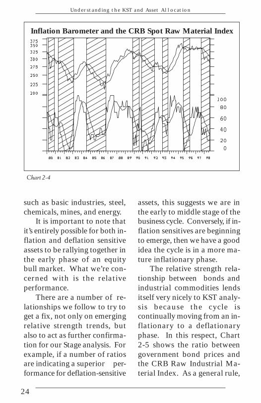
The Inflation Barometer

The Inflation Barometer,shown in Chart 2-4, is ourmost accurate model, havingidentified the majority of busi-ness cycle swings in industrialcommodity prices since the1950’s at a relatively earlystage. Changes in commodityprices are perhaps the most im-portant influence on bonds.Consequently, this indicatorhas provided us with valuableadvance warnings of reversalsin price swings in the bondmarket.

Inflation vs. Deflation

One of the most importantaspects of business-cycle analy-sis from the point of view ofoptimum asset allocation is therelationship between inflationand deflation. During themiddle to late phase of the re-cession and the early stages ofthe recovery, deflation sensitiveassets outperform inflationsensitives. Examples of defla-tion sensitive assets wouldinclude bonds and interest sen-sitive stocks such as preferedsand electric utilities. Inflationsensitive assets would embraceso called earnings driven stocks


* POSITIVE ENVIRONMENT

ENTIRE PERIOD *

NEGATIVE ENVIRONMENT *

10

25

15

20

40

5

6 8 10 12

RE

WA

RD

RISK1614

24


such as basic industries, steel,chemicals, mines, and energy.

It is important to note thatit’s entirely possible for both in-flation and deflation sensitiveassets to be rallying together inthe early phase of an equitybull market. What we’re con-cerned with is the relativeperformance.

There are a number of re-lationships we follow to try toget a fix, not only on emergingrelative strength trends, butalso to act as further confirma-tion for our Stage analysis. Forexample, if a number of ratiosare indicating a superior per-formance for deflation-sensitive

Inflation Barometer and the CRB Spot Raw Material Index

Chart 2-4

assets, this suggests we are inthe early to middle stage of thebusiness cycle. Conversely, if in-flation sensitives are beginningto emerge, then we have a goodidea the cycle is in a more ma-ture inflationary phase.

The relative strength rela-tionship between bonds andindustrial commodities lendsitself very nicely to KST analy-sis because the cycle iscontinually moving from an in-flationary to a deflationaryphase. In this respect, Chart2-5 shows the ratio betweengovernment bond prices andthe CRB Raw Industrial Ma-terial Index. As a general rule,

25

Chart 2-5

Government Bond Prices vs. CRB Raw Material Index


the long-term KST experiencesvery smooth and deliberateswings between the bull andbear phases of the cycle. Whenboth the KST and the Ratio areabove their moving averages,a relative bull market favoringinflation sensitive assets is sig-naled and vice versa. We can

also look to the position of theKST as a guide to the prevail-ing stage of the cycle. Forinstance, if the KST is over-bought and starting to rollover, it’s likely the inflationarypart of the cycle is giving wayto the deflationary part.

Chart 2-6 shows another in-

26


Chart 2-6

Inflation vs. Deflation Sensitive Groups and a Long-term KST

flation/deflation ratio. This oneis an internal stock market mea-surement since it pits an indexof inflation sensitive-equities todeflation-sensitive ones. Infla-tion-sensitives embrace stockgroups that do well when com-modity prices are rising such asmines and energy. Deflationstocks put on a superior rela-tive performance at thebeginning of the cycle as theeconomy is terminating arecessionary phase. They in-clude interest-sensitive stockssuch as electric utilities andfinancials. If you compare thisratio to the ratio betweenbonds and commodities you

will see the cyclical swings arereasonably consistent witheach other.

27

Learning the KST

"I'd recommend itto anyone." J. Bratkovich

$69.95(S/H not included)

he KST is a unique indicator which can be used by bothtraders and investors. Traders like it because it helps

identify those elusive short-term swings in the futures markets.Investors like it because it helps with those time-sensitive deci-sions within their investment portfolios. However, the most valuablefunction of the KST is its ability to provide you with perspective.

You’ve seen market-oriented commercials which make wildclaims about perfect indicators, new systems, black boxes, and soforth. The KST doesn’t need to make extravagant claims. Devel-oped more than 10 years ago, the KST system was successful inidentifying the 1990 bottom in the bond market (as featured in anarticle in the December 10, 1990 issue of Barron’s) and the 1995peak in the Deutsche mark. In Learning the KST you will discoverthe concept behind this useful indicator, together with its strengthsand weaknesses, all in more than a dozen full-color movies andaccompanying charts and illustrations.

Following the 2-hour presentation, you will find a 40-ques-tion, interactive, multimedia quiz to help you understand whatyou have learned. The automatic scoring system allows you tocompare the results of up to three tests so you can monitor yourprogress.

T

To order, please see page 3.

28


Notes

Documents

Understanding the KST and Asset Allocation - Pring … · Introduction his booklet has been provided with your ... tion within the business cycle and its importance for ... Understanding