Understanding the potential and costs for reducing UK aviation … · 2019-03-13 · electric tug taxi ..... 81 electric wheel taxi ... figure 6 open rotor fuel burn improvement by

1

ATA

Understanding the potential and costs for reducing UK aviation emissions

Report to the Committee on Climate Change and the Department for

Transport

Air Transportation Analytics Ltd and Ellondee Ltd

November 2018

2

List of revisions

Issue number

Date Reason for revision

1 November 2018 Initial Issue

Air Transportation Analytics

Air Transportation Analytics (ATA) Ltd was incorporated in May 2018 to support the aviation sector with a new level of economic and analytical capability as it addresses growth challenges. Over the past ten years, experts within ATA team with roots at University College London (UCL) and previously at the University of Cambridge, have been developing and refining a system modelling capability centred around the Aviation Integrated Modelling (AIM) project. The resulting capability can assist with sector needs on forecasting future levels of air transport demand by airline or market, identifying optimum business models for airline profit maximisation, modelling the economic and environmental implications of system and airport capacity expansion and identifying the most promising technology investment strategies of aircraft / engine manufacturers. For more details please contact Roger Gardner at [email protected] or via LinkedIn

Ellondee Ltd Ellondee Ltd’s contribution to this paper has been prepared by Martin Schofield FRAeS. Martin has worked in the civil aerospace industry for over 37 years. Graduating from Loughborough University in 1981 he spent a number of years at both British Aerospace and Deutsch Airbus in aerodynamics before moving on to broader more substantive leadership roles within the aircraft design and operations fields at Rolls-Royce and the Aerospace Technology Institute. He set up Ellondee Ltd in 2018 to act as an aircraft design and operations consultancy.

For more details please contact Martin at [email protected] or via LinkedIn

While the Committee on Climate Change (CCC) and the Department for Transport (DfT) have made every effort to ensure the information in this document is accurate, the CCC and the DfT do not guarantee the accuracy, completeness or usefulness of that information; and cannot accept liability for any loss or damages of any kind resulting from reliance on the information or guidance this document contains.

mailto:[email protected]

mailto:[email protected]

3

Although this report was commissioned by the DfT and CCC, the findings and recommendations are those of the authors and do not necessarily represent the views of the DfT or CCC. The information or guidance in this document (including third party information, products and services) is provided by DfT and the CCC on an 'as is' basis, without any representation or endorsement made and without warranty of any kind whether express or implied. The DfT and CCC have actively considered the needs of blind and partially sighted people in accessing this document. The text will be made available in full on the DfT and CCC websites. The text may be freely downloaded and translated by individuals or organisations for conversion into other accessible formats. If you have other needs in this regard please contact the DfT or CCC. Department for Transport Great Minster House 33 Horseferry Road London SW1P 4DR Telephone 0300 330 3000 General enquiries https://forms.dft.gov.uk Website www.gov.uk/dft The Committe on Climate Change 7 Holbein Place London SW1W 8NR 020 7591 6262 www.theccc.org.uk Queen’s Printer and Controller of Her Majesty’s Stationery Office, 2018, except where otherwise stated Copyright in the typographical arrangement rests with the Crown. You may re-use this information (not including logos or third-party material) free of charge in any format or medium, under the terms of the Open Government Licence v3. To view this licence, visit http://www.nationalarchives.gov.uk/doc/open-government-licence Where we have identified any third-party copyright information you will need to obtain permission from the copyright holders concerned.

https://forms.dft.gov.uk/

http://www.gov.uk/dft

http://www.theccc.org.uk/

4

Contents list

List of revisions .................................................................................................... 2

Air Transportation Analytics ................................................................................. 2

Ellondee Ltd ......................................................................................................... 2

Contents list ......................................................................................................... 4

Table of Figures ................................................................................................... 7

Table of Tables .................................................................................................... 9

Glossary ............................................................................................................ 11

1. Executive Summary ....................................................................................... 14

2. Introduction ..................................................................................................... 28

3. Task 1 – Identifying possible technological and operational changes ............ 28

3.1. Assessment of potential to change aircraft technologies ................................ 30

3.1.1. Reference aircraft types and flight lengths ............................................... 30

3.1.2. Aircraft technologies included in the assessment .................................... 30

3.1.3. Methodology used for the assessment .................................................... 31

3.1.4. Results of the assessment ....................................................................... 34

Ultra-High By-pass Ratio Turbofan (UHBR) ...................................................... 34

Open rotor ......................................................................................................... 39

Boundary Layer Ingestion (BLI) ......................................................................... 42

High Aspect ratio wing ....................................................................................... 45

Ultra-High Aspect ratio wings ............................................................................ 47

Laminar flow ...................................................................................................... 49

Natural laminar flow ........................................................................................... 51

Hybrid laminar flow ............................................................................................ 53

Electric propulsion ............................................................................................. 55

All-electric .......................................................................................................... 56

Hybrid-electric .................................................................................................... 57

Flying wing ......................................................................................................... 61

Composite materials .......................................................................................... 63

Riblets ................................................................................................................ 68

3.1.5. Summary of aircraft technologies and their likelihood of being adopted .. 70

3.2. Assessment of potential to improve airline operations ................................... 71


3.2.2. Improvement to airline operations included in the assessment ................ 72

5


3.2.4. Benefits, timing and uncertainty ............................................................... 72

Formation flying ................................................................................................. 72

Long range cruise to maximum range cruise speed/Mach ................................ 74

Aircraft design for 0.06 lower cruise Mach number ............................................ 76

Taxi out and in ................................................................................................... 79

One engine inoperative taxi ............................................................................... 80

Electric tug taxi .................................................................................................. 81

Electric wheel taxi .............................................................................................. 81

3.2.5. Summary of operational improvements and their likelihood of being adopted 83

3.3. Assessment of the potential to improve Air Traffic Management (ATM) ......... 83


3.3.2. Improvements in ATM included in the assessment .................................. 84


3.3.4. Results of the assessment ....................................................................... 85

Reduced taxi time .............................................................................................. 85

Cruise climb ....................................................................................................... 87

Optimum track ................................................................................................... 89

Continuous descent ........................................................................................... 91

Reduced contingency ........................................................................................ 93

Reduced diversion hold ..................................................................................... 95

3.3.5. Summary of air traffic management improvements and their likelihood of being adopted ....................................................................................................... 97

4. Task 2 – Estimating the value of key costs and benefits ................................ 98

4.1. Aircraft Capital Costs ...................................................................................... 99

4.2. Other Operating Cost Elements ................................................................... 100

5. Task 3 ........................................................................................................... 104

5.1. Scenario development .................................................................................. 104

5.2. Technology bundling .................................................................................... 106

5.2.1. Aircraft ................................................................................................... 107

5.2.2. Operations ............................................................................................. 108

5.2.3. Air Traffic Management .......................................................................... 108

5.2.4. Bundling method .................................................................................... 108

6. Overall results .............................................................................................. 109

6

6.1. Fuel burn changes ........................................................................................ 110

6.1.1. Aircraft ................................................................................................... 110

6.1.2. Operations ............................................................................................. 112

6.1.3. Air Traffic Management .......................................................................... 113

6.1.4. All elements combined ........................................................................... 114

6.1.5. Cost implications .................................................................................... 116

7. Quality Assurance ........................................................................................ 119

8. Bibliography .................................................................................................. 120

7

Table of Figures FIGURE 1 RELATIVE RANGE FACTOR FOR SEAT CLASSES 32 FIGURE 2 COMPARISON OF DFT AND CONSORTIUM FUEL BURNS 33 FIGURE 3 UHBR FUEL BURN IMPROVEMENT BY SEAT CLASS AND RANGE FOR THE

NOMINAL CONDITION 38 FIGURE 4: IMPACT OF CLASS 4 AND 5 CRUISE MACH NUMBER REDUCTION ON BLOCK TIMES

39 FIGURE 5: IMPACT OF CLASS 4 AND 5 CRUISE MACH NUMBER REDUCTION ON THE NUMBER

OF SECTORS FLOWN PER DAY 40 FIGURE 6 OPEN ROTOR FUEL BURN IMPROVEMENT BY SEAT CLASS AND RANGE FOR THE

NOMIONAL CONDITION 42 FIGURE 7 BLI FUEL BURN IMPROVEMENT BY SEAT CLASS AND RANGE FOR THE NOMIONAL

CONDITION 45 FIGURE 8:HIGH ASPECT RATIO FUEL BURN IMPROVEMENT BY SEAT CLASS AND RANGE

FOR THE NOMINAL CONDITION 47 FIGURE 9: ULTRA-HIGH ASPECT RATIO FUEL BURN IMPROVEMENT BY SEAT CLASS AND

RANGE FOR THE NOMINAL CONDITION 49 FIGURE 10: POTENTIAL AERODYNAMIC EFFICIENCY BENEFITS FOR LAMINAR FLOW 51 FIGURE 11:NATURAL LAMINAR FLOW FUEL BURN IMPROVEMENT BY SEAT CLASS AND

RANGE FOR THE NOMINAL CONDITION 53 FIGURE 12: VISCOUS DRAG REDUCTION AND EFFECT ON TOTAL DRAG 54 FIGURE 13:HYBRID LAMINAR FLOW FUEL BURN IMPROVEMENT BY SEAT CLASS AND RANGE

FOR THE NOMINAL CONDITION 55 FIGURE 14: ENERGY DENSITIES OF CHEMICAL FUELS AND THE BEST COMMERCIAL

BATTERY 56 FIGURE 15: PARALLEL HYBRID-ELECTRIC PROPULSION SCHEMATIC 58 FIGURE 16:HYBRID ELECTRIC PROPULSION FUEL BURN IMPROVEMENT BY SEAT CLASS

AND RANGE FOR THE NOMINAL CONDITION 60 FIGURE 17: FLYING WING FUEL BURN IMPROVEMENT BY SEAT CLASS AND RANGE FOR THE

NOMINAL CONDITION 63 FIGURE 18: AIRCRAFT COMPOSITE CONTENT BY YEAR OF INTRODUCTION 64 FIGURE 19:COMPOSITES FUEL BURN IMPROVEMENT BY SEAT CLASS AND RANGE FOR THE

NOMINAL CONDITION 68 FIGURE 20: RIBLETS FUEL BURN IMPROVEMENT BY SEAT CLASS AND RANGE FOR THE

NOMINAL CONDITION 70 FIGURE 21: PERCENTAGE TIME SPENT IN CRUISE AS A FUNCTION OF STAGE LENGTH 73 FIGURE 22:FORMATION FLYING FUEL BURN IMPROVEMENT BY SEAT CLASS AND RANGE

FOR THE NOMINAL CONDITION 74 FIGURE 23: TYPICAL COMMERCIAL TURBOFAN TRANSPORT FUEL MILEAGE AS A FUNCTION

OF MACH NUMBER, WEIGHT AT A GIVEN ALTITUDE 74 FIGURE 24: UNSMOOTHED MRC FUEL BURN IMPROVEMENT BY SEAT CLASS AND RANGE

FOR THE NOMINAL CONDITION 75 FIGURE 25: SMOOTHED MRC FUEL BURN IMPROVEMENT BY SEAT CLASS AND RANGE FOR

THE NOMINAL CONDITION 76 FIGURE 26: 0.06 REDUCTION IN CRUISE MACH NUMBER FUEL BURN IMPROVEMENT BY

SEAT CLASS AND RANGE FOR THE NOMINAL CONDITION 78 FIGURE 27:ONE ENGINE INOPERATIVE TAXI FUEL BURN IMPROVEMENT BY SEAT CLASS

AND RANGE FOR THE NOMINAL CONDITION 80 FIGURE 28: ELECTRIC TUG TAXI FUEL BURN IMPROVEMENT BY SEAT CLASS AND RANGE

FOR THE NOMINAL CONDITION 81 FIGURE 29: ELECTRIC MOTOR TAXI FUEL BURN IMPROVEMENT BY SEAT CLASS AND RANGE

FOR THE NOMINAL CONDITION 82 FIGURE 30: TYPICAL BREAKDOWN OF AN AIRCRAFT MISSION FOR PERFORMANCE

ANALYSIS PURPOSES 85 FIGURE 31:REDUCTION OF 12 MINUTES TAXI OUT AND 6 MINUTES TAXI IN BLOCK FUEL

BURN IMPROVEMENT BY SEAT CLASS AND RANGE FOR THE NOMINAL CONDITION AS CALCULATED BY PIANO-X 86

FIGURE 32: REGRESSED REDUCTION OF 18 MINUTES TAXI TIME IN BLOCK FUEL BURN IMPROVEMENT BY SEAT CLASS AND RANGE FOR THE NOMINAL CONDITION 87

8

FIGURE 33: CRUISE CLIMB PIANO-X BLOCK FUEL BURN IMPROVEMENT BY SEAT CLASS AND RANGE FOR THE NOMINAL CONDITION 88

FIGURE 34: SMOOTHED BLOCK FUEL BURN IMPROVEMENT FOR CRUISE CLIMB BY SEAT CLASS AND RANGE FOR THE NOMINAL CONDITION 89

FIGURE 35: OPTIMUM TRACK PIANO-X BLOCK FUEL BURN IMPROVEMENT BY SEAT CLASS AND RANGE FOR THE NOMINAL CONDITION 90

FIGURE 36: REGRESSED BLOCK FUEL BURN IMPROVEMENT FOR OPTIMUM TRACK BY SEAT CLASS AND RANGE FOR THE NOMINAL CONDITION 91

FIGURE 37: CONTINUOUS DESCENT PIANO-X BLOCK FUEL BURN IMPROVEMENT BY SEAT CLASS AND RANGE FOR THE NOMINAL CONDITION 92

FIGURE 38: REGRESSED BLOCK FUEL BURN IMPROVEMENT FOR CONTINUOUS DESCENT BY SEAT CLASS AND RANGE FOR THE NOMINAL CONDITION 93

FIGURE 39: REDUCED CONTINGENCY PIANO-X BLOCK FUEL BURN IMPROVEMENT BY SEAT CLASS AND RANGE FOR THE NOMINAL CONDITION 94

FIGURE 40: REGRESSED BLOCK FUEL BURN IMPROVEMENT FOR REDUCED CONTINGENCY BY SEAT CLASS AND RANGE FOR THE NOMINAL CONDITION 95

FIGURE 41: REDUCED DIVERSION HOLD PIANO-X BLOCK FUEL BURN IMPROVEMENT BY SEAT CLASS AND RANGE FOR THE NOMINAL CONDITION 96

FIGURE 42:REGRESSED BLOCK FUEL BURN IMPROVEMENT FOR REDUCED DIVERSION HOLD BY SEAT CLASS AND RANGE FOR THE NOMINAL CONDITION 97

FIGURE 43: CURRENT MARKET LANDSCAPE AND POTENTIAL TIMING OF NEW AIRCRAFT PROGRAMMES 105

FIGURE 44: EXAMPLE OF THE DIFFERENCE IN BUNDLING OUTCOME BETWEEN FACTORED AND RMS METHODS 109

FIGURE 45: POTENTIAL AIRCRAFT LEVEL BLOCK FUEL IMPROVEMENT BY 2030-2035 FOR ALL SCENARIOS AND RANGES OF DATA 110

FIGURE 46: POTENTIAL AIRCRAFT LEVEL BLOCK FUEL IMPROVEMENT BY 2045-2050 FOR ALL SCENARIOS AND RANGES OF DATA 111

FIGURE 47: POTENTIAL OPERATIONS BLOCK FUEL IMPROVEMENT BETWEEN 2030-2050 FOR ALL SCENARIOS AND RANGES OF DATA 112

FIGURE 48: POTENTIAL AIR TRAFFIC MANAGEMENT BLOCK FUEL IMPROVEMENT BETWEEN 2030-2050 FOR ALL SCENARIOS AND RANGES OF DATA 113

FIGURE 49: POTENTIAL COMBINED BLOCK FUEL IMPROVEMENT BETWEEN 2030-2035 FOR ALL SCENARIOS AND RANGES OF DATA 114

FIGURE 50: POTENTIAL COMBINED BLOCK FUEL IMPROVEMENT BETWEEN 2045-2050 FOR ALL SCENARIOS AND RANGES OF DATA 115

9

Table of Tables TABLE 1 AIRCRAFT ASSUMPTIONS FOR FUEL BURN DATA 33 TABLE 2 ICCT SFC AND WEIGHT IMPROVEMENTS FOR 2034 35 TABLE 3 ENGINE CHARACTERISTICS FOR DFT REFERENCE AIRCRAFT 35 TABLE 4 SUMMARY OF UHBR ATTRIBUTES FOR FUEL BURN ESTIMATION 37 TABLE 5 SUMMARY OF OPEN ROTOR ATTRIBUTES FOR FUEL BURN ESTIMATION 41 TABLE 6 SUMMARY OF BLI ATTRIBUTES FOR FUEL BURN ESTIMATION 44 TABLE 7:SUMMARY OF HIGH ASPECT RATIO WING ATTRIBUTES FOR FUEL BURN

ESTIMATION 47 TABLE 8: SUMMARY OF ULTRA-HIGH ASPECT RATIO WING ATTRIBUTES FOR FUEL BURN

ESTIMATION 49 TABLE 9: NASA GREEN NLF DRAG IMPROVEMENT BY AIRCRAFT COMPONENTS 51 TABLE 10: SUMMARY OF NATURAL LAMINAR FLOW ATTRIBUTES FOR FUEL BURN

ESTIMATION 52 TABLE 11: SUMMARY OF HYBRID LAMINAR FLOW ATTRIBUTES FOR FUEL BURN ESTIMATION

55 TABLE 12: HYBRID ELECTRIC AIRCRAFT WEIGHT BUILD UP 59 TABLE 13:SUMMARY OF HYBRID ELECTRIC PROPULSION ATTRIBUTES FOR FUEL BURN

ESTIMATION 60 TABLE 14: SUMMARY OF FLYING WING ATTRIBUTES FOR FUEL BURN ESTIMATION 62 TABLE 15: WEIGHT SAVINGS FOR COMPOSITE BY DIFFERENT COMPONENT TYPES 65 TABLE 16: COMPONENT GROUP WEIGHTS RELATIVE TO MAXIMUM TAKE-OFF WEIGHT BY

SEAT CLASS 65 TABLE 17: COMPOSITE AIRFRAME WEIGHT BENEFITS BY SEAT CLASS 66 TABLE 18: 2 SHAFT ENGINE RELATIVE WEIGHT BREAKDOWN 66 TABLE 19: 3 SHAFT ENGINE RELATIVE WEIGHT BREAKDOWN 66 TABLE 20: COMPOSITE ENGINE WEIGHT SAVINGS BY SEAT CLASS 67 TABLE 21: SUMMARY OF COMPOSITE ATTRIBUTES FOR FUEL BURN ESTIMATION 68 TABLE 22: AIRFRAME COMPONENT DRAG REDUCTIONS FOR RIBLETS 69 TABLE 23: FUSELAGE AND TAIL PAINT WEIGHTS FOR DIFFERENT SEAT CLASSES 69 TABLE 24: SUMMARY OF RIBLET ATTRIBUTES FOR FUEL BURN ESTIMATION 70 TABLE 25: SUMMARY OF AIRCRAFT TECHNOLOGY BENEFITS, ENTRY INTO SERVICE DATES

AND LIKELIHOODS 71 TABLE 26: MIT ESTIMATION OF CHANGE IN WEIGHT, DRAG AND SFC WITH REDUCING MACH

NUMBER 77 TABLE 27: NASA ESTIMATION OF CHANGE IN WEIGHT, DRAG AND SFC WITH REDUCING

MACH NUMBER 77 TABLE 28: MAIN ENGINE AND APU TAXI FUEL FLOWS FOR THE DFT SEAT CLASSES 79 TABLE 29: SUMMARY OF OPERATIONAL IMPROVEMENT BENEFITS, ENTRY INTO SERVICE

DATES AND LIKELIHOODS 83 TABLE 30: REGRESSION COEFFICIENTS FOR BLOCK FUEL BURN REDUCTION WITH

REDUCED TAXI TIME 86 TABLE 31:EQUATION COEFFICIENTS FOR BLOCK FUEL BURN REDUCTION FOR CRUISE

CLIMB 88 TABLE 32: REGRESSION COEFFICIENTS FOR BLOCK FUEL BURN REDUCTION FOR OPTIMUM

TRACK 90 TABLE 33: REGRESSION COEFFICIENTS FOR BLOCK FUEL BURN REDUCTION FOR

CONTINUOUS DESCENT 92 TABLE 34: REGRESSION COEFFICIENTS FOR BLOCK FUEL BURN REDUCTION FOR

REDUCED CONTINGENCY 94 TABLE 35:REGRESSION COEFFICIENTS FOR BLOCK FUEL BURN REDUCTION FOR REDUCED

DIVERSION HOLD 96 TABLE 36: SUMMARY OF AIR TRAFFIC MANAGEMENT IMPROVEMENT BENEFITS, ENTRY

INTO SERVICE DATES AND LIKELIHOODS 98 TABLE 37: ESTIMATED ENGINE LIST PRICE MODEL 100 TABLE 38: FORM 41 SCHEDULES USED FOR DOC COMPONENTS 101 TABLE 39: REQUIRED EXPLANATORY VARIABLES FROM SCHEDULE T2 102

10

TABLE 40: ADDITIONAL REQUIRED EXPLANATORY VARIABLES 102 TABLE 41: CREW COSTS 103 TABLE 42: AIRFRAME MAINTENANCE 103 TABLE 43: ENGINE MAINTENANCE 103 TABLE 44: OTHER EXPENDITURES 104 TABLE 45:TIME BETWEEN MAJOR DERIVATIVES FOR CLASSES 2,3 AND 5 105 TABLE 46: TECHNOLOGY IMPLEMENTATION TABLE FOR THE THREE SCENARIOS 107 TABLE 47: AVERAGE FUEL BURN REDUCTIONS FOR AIRCRAFT TECHNOLOGIES IN 2030-2035

111 TABLE 48: AVERAGE FUEL BURN REDUCTIONS FOR AIRCRAFT TECHNOLOGIES IN 2045-2050

111 TABLE 49: AVERAGE FUEL BURN REDUCTIONS FOR OPERATIONAL IMPROVEMENTS IN 2030-

2050 113 TABLE 50: AVERAGE FUEL BURN REDUCTIONS FOR AIR TRAFFIC MANAGEMENT

IMPROVEMENTS IN 2030-2050 114 TABLE 51: AVERAGE FUEL BURN REDUCTIONS FOR ALL IMPROVEMENTS IN 2030-2035 115 TABLE 52: AVERAGE FUEL BURN REDUCTIONS FOR ALL IMPROVEMENTS IN 2045-2050 116 TABLE 53: DIRECT OPERATING COSTS FOR THE REFERENCE AIRCRAFT AND THE

PROJECTED FUTURE VEHICLES FOR THE WORST CASE OF THE LIKELY SCENARIO 117 TABLE 54: DIRECT OPERATING COSTS FOR THE REFERENCE AIRCRAFT AND THE

PROJECTED FUTURE VEHICLES FOR THE NOMINAL CASE OF THE LIKELY SCENARIO 117

TABLE 55: DIRECT OPERATING COSTS FOR THE REFERENCE AIRCRAFT AND THE PROJECTED FUTURE VEHICLES FOR THE BEST CASE OF THE LIKELY SCENARIO 118

TABLE 56: DISCOUNTED CO2 MITIGATION COSTS FOR THE WORST, NOMINAL AND OPTIMISTIC CASE OF THE LIKELY SCENARIO IN £(2015) 118

11

Glossary Aircraft weights. Empty weight is the weight of the aircraft with neither fuel nor payload loaded. Zero fuel weight is the weight of the aircraft with no fuel onboard and with the payload loaded. Take-off weight is the aircraft weight at the start of take-off and is the sum of the empty weight, payload and fuel required to complete the mission including any reserves. Landing weight is the weight of the aircraft having burnt off the fuel to arrive at its destination.

Assessment range covers three possible outcomes for the attributes of each technology. Worst is the lowest level of attribute change: Nominal is expected level of attribute change: Best is the highest level of attribute change. Three scenario options have been created. Pessimistic uses only the most obvious high value low challenge technologies: Likely adopts the most likely technologies based on the current well-developed technology plans: Optimistic introduces some high-risk technologies in addition to the technologies adopted in the “likely” case.

Available seat miles defines the capability of an aircraft type to serve a given airline market and is the number of seats in an aircraft multiplied by the distance flown on all the routes it is used on. Baseline refers to the reference aircraft defined with the DfT seat classes and links the aerodynamic, weight or engine efficiency standard of those aircraft to the changes identified in each technology.

Breguet range equation is algebraically developed from fundamental aeronautics principles to define the aircraft’s range capability as a function of aircraft weights, speed, aerodynamic and engine efficiencies. Drag is the aerodynamic force that opposes the motion of the aircraft through the air. It is made up of a number of components, the key ones used in this document are: Skin friction drag is created by the contact of the aircraft skin with the air and is a consequence of the air’s viscosity: Induced drag is created as the consequence of generating lift: Total drag is the sum of all drag components on the aircraft including skin friction and induced drag. Interference drag is any drag created by the aerodynamic influence of one surface to another when in close proximity. Parasitic drag is created by steps and gaps in the surface caused during design or manufacture. Aerials and antennae are also sources of parasitic drag.

Engine accessories covers components required by the aircraft and powered from the engine. Examples include starter motors, hydraulic pumps and electric generators.

Engine weights uses two separate definitions. Dry weight relates to the engine without nacelle and its associated components or mounting structure or without fluids. Powerplant system (PPS) weight is the dry weight plus the weights for the nacelle and its associated components and mounting structure and with residual fluids.

En-route covers any part of the mission above altitudes of more than 1,500 ft from either the departing or arriving airport.

12

Entry into service is the date when the first revenue service of a new aircraft type occurs.

Fixed is a term to describe a fuel burn change when technologies have been applied to the aircraft but the rest of the aircraft does not change its physical size.

Snowballed is when the aircraft’s physical size is allowed to change to take further advantage of the attributes of the technological change in addition to the benefits brought by the technology itself.

Flight time is the time taken to fly the mission from the point at which the aircraft leaves the ground to the point at which it touches the ground again. Block time is flight time with the addition of the time taken from the moment the aircraft leaves the gate to the moment it returns to the gate.

Fuel burn is the amount of fuel burnt on a mission. Trip fuel is the fuel burnt on the mission from the point at which the aircraft leaves the ground to the point at which it touches the ground again. Block fuel is trip fuel with the addition of the fuel burnt from the moment the aircraft leaves the gate to the moment it returns to the gate.

Great circle distance is the shortest distance between any two points on the earth’s surface measured along the surface.

Lift to drag ratio is a measure of aerodynamic efficiency. The lift is the required output and the resultant drag is the consequence of this output.

Local air quality looks at aircraft emissions such as CO2, NOx, unburnt hydrocarbons and smoke in the airport environment.

Mach number is the ratio of the aircraft’s speed relative to the local speed of sound.

Mission. A flight from an origin to a destination is a mission. The distance flown on this mission can be termed either stage length or range.

Noise. Aircraft noise near the airport is assessed by the certification authorities at three precisely defined points. Take-off – sideline is to the side of the runway during the take-off run. Take-off – cutback is underneath the aircraft once it has lifted off and approach is underneath the aircraft as it approaches to land.

Payload is the weight of the passenger their bags and any additional cargo.

Primary structures are structures that carry flight and ground loads, and whose failure would reduce the structural integrity of the aircraft. Secondary structures are the other structures and their failure would not reduce the structural integrity of the airframe.

Propulsor is a generic term to cover any unit that generates propulsive thrust.

Reserves defines extra fuel carried on the flight to allow for unforeseen circumstances during the flight. Examples include the need to divert away from the destination airport or encountering more severe headwinds than forecast.

13

Specific fuel consumption is a term reflecting the efficiency of a hydrocarbon powered engine. It is the ratio of the amount of thrust being generated (as the output) per unit of fuel being consumed in a given time (as the input).

Strut is a beam that runs between a point along the wing span on the lower surface of the wing and the aircraft fuselage to increase the wing’s stiffness.

Technology Readiness Level is a sliding scale of technology maturity (from 0 to 9) with the higher the level the higher the confidence to apply the technology in a production ready piece of equipment.

Utilisation is the number of flying hours per year that an aircraft achieves.

Wing planform is the shape of the wing when looking down from above.

Wing section is the shape of the upper and lower surface of the wing when a slice has been taken through the wing parallel to the line of flight.

Wing sweep is angle of the wing in relation to the local flow when looking down on the wing from above.

14

1. Executive Summary This research was commissioned by the Committee on Climate Change (the CCC) and the Department for Transport (the DfT) to review the potential for reductions in CO2 emissions from prospective and potential changes to aircraft technology, air traffic management and airline operations. The CCC has previously published advice to the government on how UK aviation emissions could be reduced. References [1] and [2] are based on detailed modelling of the technologies and behaviours that could be deployed. Given the legally-binding targets set by the Climate Change Act, the CCC and the DfT are interested to update advice on potential for aviation emissions reduction, in advance of the planned launch of a new Aviation Strategy in 2019. The research undertaken by the Consortium (Air Transportation Analytics Ltd (ATA) with support from Ellondee Ltd) comprised three tasks:

• First, it examined and quantified the full range of major plausible changes in technology, air traffic management and operational measures that could be made to reduce fuel consumption and CO2 emissions from aviation to 2050 and beyond.

• Second, it estimated the key costs and benefits that could arise from implementation of the identified options.

• Finally, the DfT central scenario for aviation fuel efficiency, air traffic management, and operations improvement was reviewed and additional scenarios produced.

To understand the way in which these technologies may be introduced, timescales have been proposed for new aircraft type introduction. Technology bundles have been created for these new aircraft types and the technology benefits aggregated. Aircraft Technology Changes In consultation with the CCC and the DfT, representative aircraft in each of the 4 central aircraft size (seat class) categories within the DfT aviation model were selected as a baseline for considering technology change. These represent the largest use of aircraft on an available seat miles basis (ASM) from UK airports and are:

• Class 2 (71 to 150 seats): Bombardier DHC8-Q400 (flight length from 125 to 1,500 nautical miles (nm) or Airbus A319CEO (flight length from 125 to 3,000 nm)

• Class 3 (151 to 250 seats): Airbus A320CEO (flight length from 125 to 2,500 nm)

• Class 4 (250 to 350 seats): Boeing 777-200ER (flight length from 125 to 7,500 nm)

• Class 5 (350 to 500 seats): Boeing 747-400 (flight length from 125 to 7,000 nm)

15

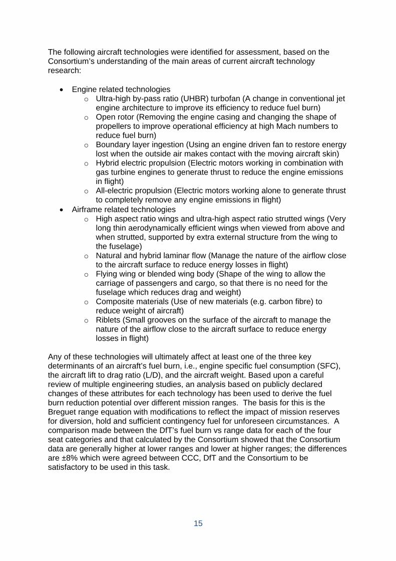
The following aircraft technologies were identified for assessment, based on the Consortium’s understanding of the main areas of current aircraft technology research:

• Engine related technologies o Ultra-high by-pass ratio (UHBR) turbofan (A change in conventional jet

engine architecture to improve its efficiency to reduce fuel burn) o Open rotor (Removing the engine casing and changing the shape of

propellers to improve operational efficiency at high Mach numbers to reduce fuel burn)

o Boundary layer ingestion (Using an engine driven fan to restore energy lost when the outside air makes contact with the moving aircraft skin)

o Hybrid electric propulsion (Electric motors working in combination with gas turbine engines to generate thrust to reduce the engine emissions in flight)

o All-electric propulsion (Electric motors working alone to generate thrust to completely remove any engine emissions in flight)

• Airframe related technologies o High aspect ratio wings and ultra-high aspect ratio strutted wings (Very

long thin aerodynamically efficient wings when viewed from above and when strutted, supported by extra external structure from the wing to the fuselage)

o Natural and hybrid laminar flow (Manage the nature of the airflow close to the aircraft surface to reduce energy losses in flight)

o Flying wing or blended wing body (Shape of the wing to allow the carriage of passengers and cargo, so that there is no need for the fuselage which reduces drag and weight)

o Composite materials (Use of new materials (e.g. carbon fibre) to reduce weight of aircraft)

o Riblets (Small grooves on the surface of the aircraft to manage the nature of the airflow close to the aircraft surface to reduce energy losses in flight)

Any of these technologies will ultimately affect at least one of the three key determinants of an aircraft’s fuel burn, i.e., engine specific fuel consumption (SFC), the aircraft lift to drag ratio (L/D), and the aircraft weight. Based upon a careful review of multiple engineering studies, an analysis based on publicly declared changes of these attributes for each technology has been used to derive the fuel burn reduction potential over different mission ranges. The basis for this is the Breguet range equation with modifications to reflect the impact of mission reserves for diversion, hold and sufficient contingency fuel for unforeseen circumstances. A comparison made between the DfT’s fuel burn vs range data for each of the four seat categories and that calculated by the Consortium showed that the Consortium data are generally higher at lower ranges and lower at higher ranges; the differences are ±8% which were agreed between CCC, DfT and the Consortium to be satisfactory to be used in this task.

16

Three important factors underpinning the analysis are:

• Alterations in one aircraft component will affect others. For example, enhanced use of lightweight materials will result in a lighter airframe, thus requiring smaller engines, a lighter landing gear, less fuel to be carried on board, etc. for the same mission. In this study, the analysis accounted for these propagating or snowball effects by increasing the overall fuel burn benefit by between 20 and 30%.

• To account for the uncertainty associated with the performance of future aircraft technology, the analysis used plausible ranges of literature estimates to form a central (“nominal”) estimate with a lower and upper bound (“worst” and “best”). Entry into service (EIS) dates have been noted where found in literature searches to help define which technologies will be mature enough to be included on new aircraft and by when.

• The modelling assumes that the most promising individual technologies are bundled together into new aircraft types, once they are sufficiently mature (to at least Technology Readiness Level 6).

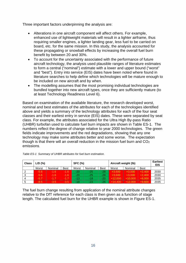
Based on examination of the available literature, the research developed worst, nominal and best estimates of the attributes for each of the technologies identified above and yields a summary of the technology attributes for each of the four seat classes and their earliest entry in service (EIS) dates. These were separated by seat class. For example, the attributes associated for the Ultra High By-pass Ratio (UHBR) turbofan used to calculate fuel burn impacts are shown in Table ES-1. The numbers reflect the degree of change relative to year 2000 technologies. The green fields indicate improvements and the red degradations, showing that any one technology may make some attributes better and some worse. The expectation though is that there will an overall reduction in the mission fuel burn and CO2 emissions. Table ES-1 Summary of UHBR attributes for fuel burn estimation.

Class L/D (%) SFC (%) Aircraft weight (lb) Earliest EIS

Worst Nominal Best Worst Nominal Best Worst Nominal Best 2 -5.6 -1.6 -1.6 -20 -25 -28 +3,600 +3,000 +2,400 2030 3 -5.6 -1.6 -1.6 -20 -25 -28 +3,600 +3,000 +2,400 2030 4 -5.7 -1.7 -1.7 -13 -18 -20 +12,000 +10,000 +8,000 2035 5 -8.5 -3.5 -3.5 -18 -23 -26 +14,400 +12,000 +9,600 2035

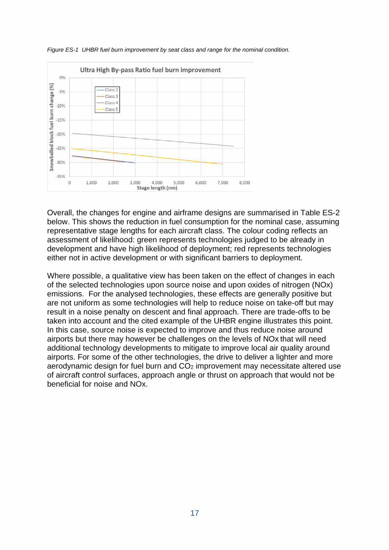
The fuel burn change resulting from application of the nominal attribute changes relative to the DfT reference for each class is then given as a function of stage length. The calculated fuel burn for the UHBR example is shown in Figure ES-1.

17

Figure ES-1 UHBR fuel burn improvement by seat class and range for the nominal condition.

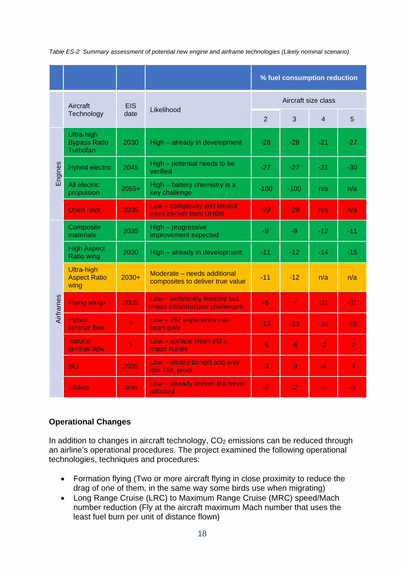
Overall, the changes for engine and airframe designs are summarised in Table ES-2 below. This shows the reduction in fuel consumption for the nominal case, assuming representative stage lengths for each aircraft class. The colour coding reflects an assessment of likelihood: green represents technologies judged to be already in development and have high likelihood of deployment; red represents technologies either not in active development or with significant barriers to deployment. Where possible, a qualitative view has been taken on the effect of changes in each of the selected technologies upon source noise and upon oxides of nitrogen (NOx) emissions. For the analysed technologies, these effects are generally positive but are not uniform as some technologies will help to reduce noise on take-off but may result in a noise penalty on descent and final approach. There are trade-offs to be taken into account and the cited example of the UHBR engine illustrates this point. In this case, source noise is expected to improve and thus reduce noise around airports but there may however be challenges on the levels of NOx that will need additional technology developments to mitigate to improve local air quality around airports. For some of the other technologies, the drive to deliver a lighter and more aerodynamic design for fuel burn and CO2 improvement may necessitate altered use of aircraft control surfaces, approach angle or thrust on approach that would not be beneficial for noise and NOx.

18

Table ES-2 Summary assessment of potential new engine and airframe technologies (Likely nominal scenario)

% fuel consumption reduction

Aircraft Technology

EIS date Likelihood

Aircraft size class

2 3 4 5

Engi

nes

Ultra-high Bypass Ratio Turbofan

2030 High – already in development -28 -28 -21 -27

Hybrid electric 2045 High – potential needs to be verified -27 -27 -31 -30

All electric propulsion 2055+ High – battery chemistry is a

key challenge -100 -100 n/a n/a

Open rotor 2035 Low – complexity and limited extra benefit from UHBR -29 -29 n/a n/a

Airfr

ames

Composite materials 2035 High – progressive

improvement expected -9 -9 -12 -11

High Aspect Ratio wing 2030 High – already in development -11 -12 -14 -15

Ultra-high Aspect Ratio wing

2030+ Moderate – needs additional composites to deliver true value -11 -12 n/a n/a

Flying wings 2035 Low – technically feasible but major infrastructure challenges -6 -7 -31 -31

Hybrid laminar flow ? Low – 787 experience has

been poor -13 -13 -10 -10

Natural laminar flow ? Low – surface finish still a

major hurdle -6 -6 -2 -2

BLI 2035 Low – limited benefit and only low TRL proof -3 -3 -4 -4

Riblets Now Low – already proven but never adopted -2 -2 -3 -3

Operational Changes In addition to changes in aircraft technology, CO2 emissions can be reduced through an airline’s operational procedures. The project examined the following operational technologies, techniques and procedures:

• Formation flying (Two or more aircraft flying in close proximity to reduce the drag of one of them, in the same way some birds use when migrating)

• Long Range Cruise (LRC) to Maximum Range Cruise (MRC) speed/Mach number reduction (Fly at the aircraft maximum Mach number that uses the least fuel burn per unit of distance flown)

19

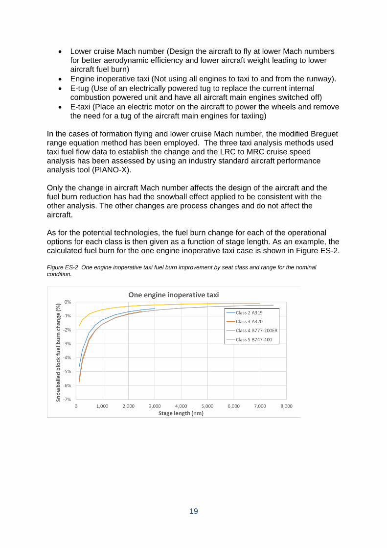
• Lower cruise Mach number (Design the aircraft to fly at lower Mach numbers for better aerodynamic efficiency and lower aircraft weight leading to lower aircraft fuel burn)

• Engine inoperative taxi (Not using all engines to taxi to and from the runway). • E-tug (Use of an electrically powered tug to replace the current internal

combustion powered unit and have all aircraft main engines switched off) • E-taxi (Place an electric motor on the aircraft to power the wheels and remove

the need for a tug of the aircraft main engines for taxiing) In the cases of formation flying and lower cruise Mach number, the modified Breguet range equation method has been employed. The three taxi analysis methods used taxi fuel flow data to establish the change and the LRC to MRC cruise speed analysis has been assessed by using an industry standard aircraft performance analysis tool (PIANO-X). Only the change in aircraft Mach number affects the design of the aircraft and the fuel burn reduction has had the snowball effect applied to be consistent with the other analysis. The other changes are process changes and do not affect the aircraft. As for the potential technologies, the fuel burn change for each of the operational options for each class is then given as a function of stage length. As an example, the calculated fuel burn for the one engine inoperative taxi case is shown in Figure ES-2. Figure ES-2 One engine inoperative taxi fuel burn improvement by seat class and range for the nominal condition.

20

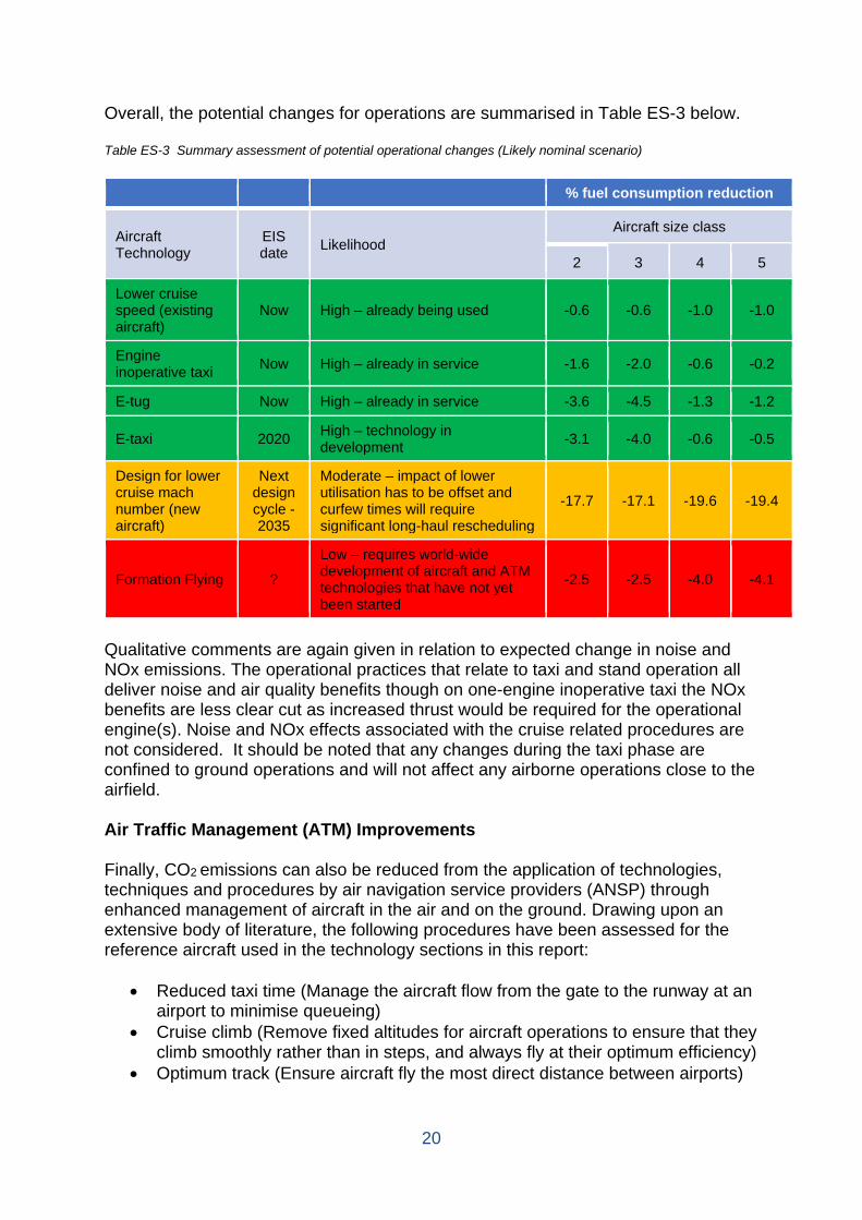
Overall, the potential changes for operations are summarised in Table ES-3 below. Table ES-3 Summary assessment of potential operational changes (Likely nominal scenario)


Aircraft Technology

EIS date Likelihood

Aircraft size class

2 3 4 5

Lower cruise speed (existing aircraft)

Now High – already being used -0.6 -0.6 -1.0 -1.0

Engine inoperative taxi Now High – already in service -1.6 -2.0 -0.6 -0.2

E-tug Now High – already in service -3.6 -4.5 -1.3 -1.2

E-taxi 2020 High – technology in development -3.1 -4.0 -0.6 -0.5

Design for lower cruise mach number (new aircraft)

Next design cycle -2035

Moderate – impact of lower utilisation has to be offset and curfew times will require significant long-haul rescheduling

-17.7 -17.1 -19.6 -19.4

Formation Flying ?

Low – requires world-wide development of aircraft and ATM technologies that have not yet been started

-2.5 -2.5 -4.0 -4.1

Qualitative comments are again given in relation to expected change in noise and NOx emissions. The operational practices that relate to taxi and stand operation all deliver noise and air quality benefits though on one-engine inoperative taxi the NOx benefits are less clear cut as increased thrust would be required for the operational engine(s). Noise and NOx effects associated with the cruise related procedures are not considered. It should be noted that any changes during the taxi phase are confined to ground operations and will not affect any airborne operations close to the airfield. Air Traffic Management (ATM) Improvements Finally, CO2 emissions can also be reduced from the application of technologies, techniques and procedures by air navigation service providers (ANSP) through enhanced management of aircraft in the air and on the ground. Drawing upon an extensive body of literature, the following procedures have been assessed for the reference aircraft used in the technology sections in this report:

• Reduced taxi time (Manage the aircraft flow from the gate to the runway at an airport to minimise queueing)

• Cruise climb (Remove fixed altitudes for aircraft operations to ensure that they climb smoothly rather than in steps, and always fly at their optimum efficiency)

• Optimum track (Ensure aircraft fly the most direct distance between airports)

21

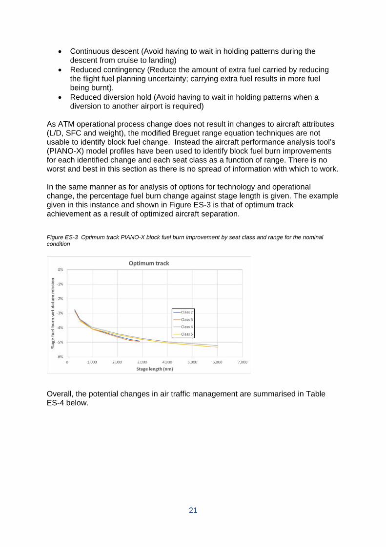
• Continuous descent (Avoid having to wait in holding patterns during the descent from cruise to landing)

• Reduced contingency (Reduce the amount of extra fuel carried by reducing the flight fuel planning uncertainty; carrying extra fuel results in more fuel being burnt).

• Reduced diversion hold (Avoid having to wait in holding patterns when a diversion to another airport is required)

As ATM operational process change does not result in changes to aircraft attributes (L/D, SFC and weight), the modified Breguet range equation techniques are not usable to identify block fuel change. Instead the aircraft performance analysis tool’s (PIANO-X) model profiles have been used to identify block fuel burn improvements for each identified change and each seat class as a function of range. There is no worst and best in this section as there is no spread of information with which to work. In the same manner as for analysis of options for technology and operational change, the percentage fuel burn change against stage length is given. The example given in this instance and shown in Figure ES-3 is that of optimum track achievement as a result of optimized aircraft separation. Figure ES-3 Optimum track PIANO-X block fuel burn improvement by seat class and range for the nominal condition

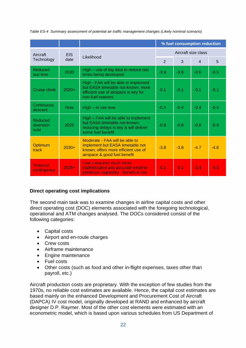
Overall, the potential changes in air traffic management are summarised in Table ES-4 below.

22

Table ES-4 Summary assessment of potential air traffic management changes (Likely nominal scenario)


Aircraft Technology

EIS date Likelihood

Aircraft size class

2 3 4 5

Reduced taxi time 2030 High – use of big data to reduce taxi

times being developed -3.9 -3.8 -0.6 -0.5

Cruise climb 2020+

High - FAA will be able to implement but EASA timetable not known; more efficient use of airspace is key for non-fuel reasons

-0.1 -0.1 -0.1 -0.1

Continuous descent Now High – in use now -0.4 -0.4 -0.4 -0.4

Reduced diversion hold

2025

High – FAA will be able to implement but EASA timetable not known; reducing delays is key & will deliver some fuel benefit

-0.9 -0.8 -0.8 -0.9

Optimum track 2030+

Moderate - FAA will be able to implement but EASA timetable not known; offers more efficient use of airspace & good fuel benefit

-3.8 -3.8 -4.7 -4.8

Reduced contingency 2025+

Low – requires much more sophisticated and accurate weather prediction capability. Benefit is low

-0.1 -0.1 -0.4 -0.5

Direct operating cost implications The second main task was to examine changes in airline capital costs and other direct operating cost (DOC) elements associated with the foregoing technological, operational and ATM changes analysed. The DOCs considered consist of the following categories:

• Capital costs • Airport and en-route charges • Crew costs • Airframe maintenance • Engine maintenance • Fuel costs • Other costs (such as food and other in-flight expenses, taxes other than

payroll, etc.) Aircraft production costs are proprietary. With the exception of few studies from the 1970s, no reliable cost estimates are available. Hence, the capital cost estimates are based mainly on the enhanced Development and Procurement Cost of Aircraft (DAPCA) IV cost model, originally developed at RAND and enhanced by aircraft designer D.P. Raymer. Most of the other cost elements were estimated with an econometric model, which is based upon various schedules from US Department of

23

Transport (D.O.T) Form 41 data that US airlines are required to submit on financial and operating information. The enhanced DAPCA IV model employs aircraft empty weight, maximum aircraft speed, maximum engine thrust and the number of aircraft produced as key determinants of aircraft capital cost. The model estimates the non-recurring (development and validation) costs and the recurring (production) costs of airframes using statistical relationships for engineering, tooling, manufacturing and quality control. For aircraft largely relying on other materials than aluminium, some cost elements are adjusted with material-specific correction factors. The DAPCA IV model provides estimation relationships for engine prices depending on engine thrust, maximum Mach number, turbine inlet temperature and production quantity. On account of difficulties in accessing turbine inlet temperature data for modern engines, ATA developed a different engine price model which explains the engine list price as a function of maximum thrust, cruise engine specific fuel consumption and certification year and then applied typical discounts to arrive at the engine research and technology and production costs. Following this approach, capital costs of all anticipated future aircraft are projected to increase over those of the reference aircraft because of the assumed high content of carbon-fibre composites and higher engine costs. The method employed for estimating DOC components other than capital costs is based mainly upon an econometric model of U.S. Form 41 economic and operations data. These data were complemented with additional explanatory variables from other identified sources. Whereas DOC costs associated with flight crew were assumed to remain unchanged, those describing airframe and engine maintenance, airport/en-route charges and fuel expenditures are projected to decrease because of the beneficial effects of the technologies, which include mainly lower aircraft weight, lower-thrust engines and reduced aircraft fuel consumption in general. Scenario analysis As well as reviewing the DfT central scenario, the project created three additional scenarios that were considered and agreed with the CCC and the DfT. These scenarios were quantified out to 2050 in a form suitable for inclusion in the DfT aviation model. The civil aircraft manufacturing sector usually takes a number of technologies and “bundles” them into the next aircraft design to show a significant fuel burn and cash operating cost improvement relative to the current in-service types. The appetite for airlines to migrate to a higher level “bundled” product is also affected by the competitive landscape and the report assumes that new aircraft are introduced every 15 years in each seat class. The current market place has seen major derivatives introduced such as the A320NEO in 2016 and the B737MAX family in 2017 which suggests that new programmes are unlikely to be introduced before 2030. Similar new aircraft introductions and outcomes are visible for key aircraft families in seat classes 4 and 5. Given the timing of key aircraft programmes in their development cycle and the typical 7-year development timeline for new aircraft and a typical 15-year timespan

24

between introduction of new aircraft designs, it was concluded that there will be two new aircraft cycles between now and 2050 for each seat class:

• Seat classes 2 and 3: 2030 and 2045 • Seat classes 4 and 5: 2035 and 2050

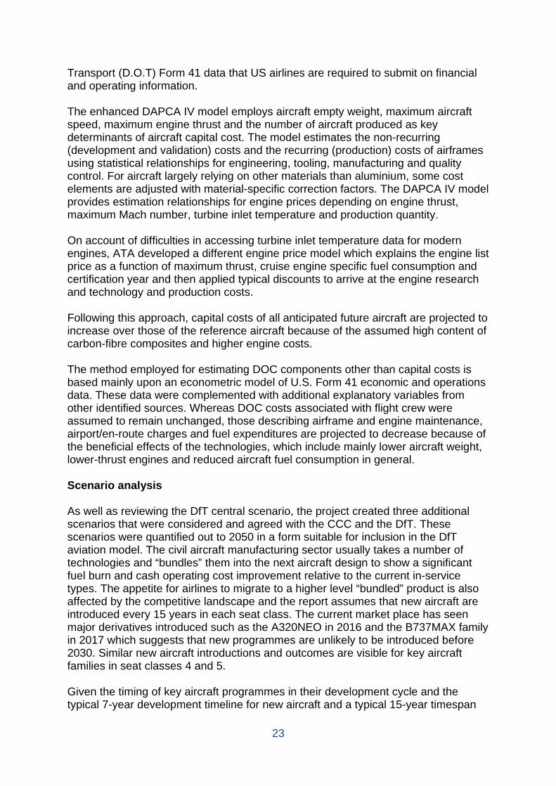
Technology bundling The technology analysis task has defined aircraft, air traffic management and operational technologies, techniques and procedural changes and quantified them in terms of fuel burn improvement and likely entry into service date. In conjunction with CCC and DfT, three definitions have been established that allow the likelihood of adoption that, in conjunction with the entry into service date, can be mapped into detailed scenarios. These definitions are:

• Pessimistic – only the most obvious high-value low-challenge technologies are adopted

• Likely – the most likely technologies are adopted based on the current well-developed technology plans

• Optimistic – some high-risk technologies are adopted in addition to the “Likely” case

Table ES-5 shows the technology content of these three scenarios. Table ES-5 Technology content of the Pessimistic, Likely and Optimistic Scenario

25

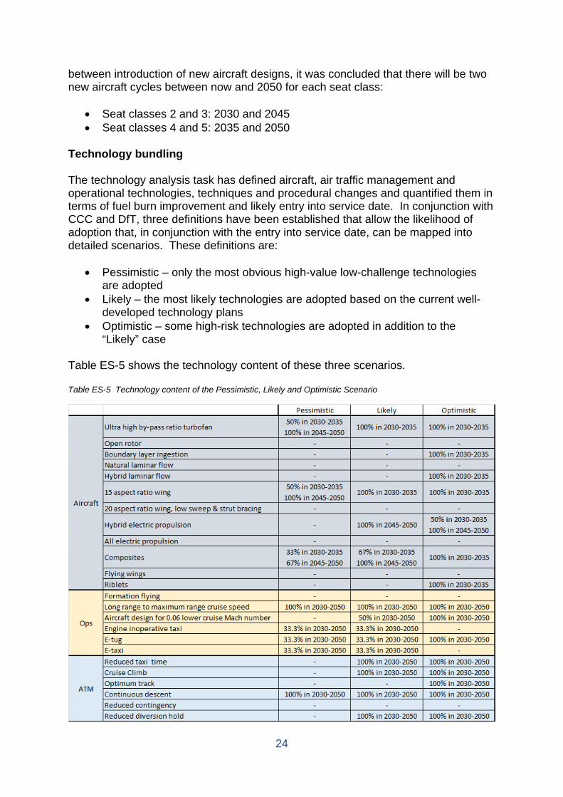
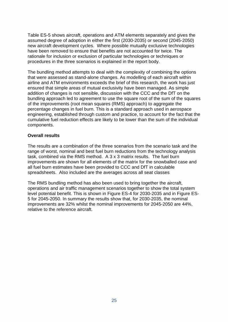
Table ES-5 shows aircraft, operations and ATM elements separately and gives the assumed degree of adoption in either the first (2030-2035) or second (2045-2050) new aircraft development cycles. Where possible mutually exclusive technologies have been removed to ensure that benefits are not accounted for twice. The rationale for inclusion or exclusion of particular technologies or techniques or procedures in the three scenarios is explained in the report body. The bundling method attempts to deal with the complexity of combining the options that were assessed as stand-alone changes. As modelling of each aircraft within airline and ATM environments exceeds the brief of this research, the work has just ensured that simple areas of mutual exclusivity have been managed. As simple addition of changes is not sensible, discussion with the CCC and the DfT on the bundling approach led to agreement to use the square root of the sum of the squares of the improvements (root mean squares (RMS) approach) to aggregate the percentage changes in fuel burn. This is a standard approach used in aerospace engineering, established through custom and practice, to account for the fact that the cumulative fuel reduction effects are likely to be lower than the sum of the individual components. Overall results The results are a combination of the three scenarios from the scenario task and the range of worst, nominal and best fuel burn reductions from the technology analysis task, combined via the RMS method. A 3 x 3 matrix results. The fuel burn improvements are shown for all elements of the matrix for the snowballed case and all fuel burn estimates have been provided to CCC and DfT in calculable spreadsheets. Also included are the averages across all seat classes The RMS bundling method has also been used to bring together the aircraft, operations and air traffic management scenarios together to show the total system level potential benefit. This is shown in Figure ES-4 for 2030-2035 and in Figure ES-5 for 2045-2050. In summary the results show that, for 2030-2035, the nominal improvements are 32% whilst the nominal improvements for 2045-2050 are 44%, relative to the reference aircraft.

26

Figure ES-4 Potential combined block fuel improvement between 2030-2035.

Figure ES-5 Potential combined block fuel improvement between 2045-2050.

The resulting DOCs by category for the reference aircraft and the projected 2030-2035 and 2045-2050 period are shown in the report by cost category and aircraft seat class (see Tables 53-55). Irrespective of the scenario, the DOC of all future designs in all scenarios are projected to be below those of reference aircraft if assuming a jet fuel price of £(2015) 1.3 per gallon, in line with the BEIS fossil fuel price projections. This is the result of two contrasting trends, i.e., a decline in operating costs (predominantly fuel costs due to the higher fuel efficiency of future designs) which dominates an increase in capital costs (due to the more expensive fuel-saving technology employed). In addition, airport & en-route charges are also expected to slightly decline due to the declining aircraft weight. Similarly, airframe maintenance is projected to decline, mainly because of a time trend of -0.1%/yr and engine maintenance is projected to be lower because of the lower thrust levels required for lighter-weight aircraft.

-60%

-50%

-40%

-30%

-20%

-10%

0%

Pess

imist

ic

Like

ly

Opt

imist

ic

Pess

imist

ic

Like

ly

Opt

imist

ic

Pess

imist

ic

Like

ly

Opt

imist

ic

Pess

imist

ic

Like

ly

Opt

imist

ic

Class 2 Class 3 Class 4 Class 5

2030-35 - all improvements

-70%

-60%

-50%

-40%

-30%

-20%

-10%

0%

Pess

imist

ic

Like

ly

Opt

imist

ic

Pess

imist

ic

Like

ly

Opt

imist

ic

Pess

imist

ic

Like

ly

Opt

imist

ic

Pess

imist

ic

Like

ly

Opt

imist

ic


2045-50 - all improvements

27

Because the estimated DOCs of the projected aircraft designs are below those of the reference vehicles, the CO2 mitigation costs will be negative. According to Table ES-6, the discounted mitigation costs are projected to be in the order of -50 to -100 £(2015) per tonne of CO2 in the nominal case of the likely scenario, depending on the aircraft size class and time frame. These numbers are based on a social discount rate of 3.5%. Slightly lower (higher) values result for the Worst (Optimistic) case. If, instead, a private-sector discount rate of 10% is used, the discounted value of the mitigation costs increase but remain negative. These range from -4£(2015) per tonne of CO2 in the Worst case for Class 5 aircraft in 2050 to -42£(2015) per tonne of CO2 in the Best case for Class 2 and 3 aircraft in 2030. Table ES-6 Discounted CO2 mitigation costs in £(2015)/tCO2 in the Likely Scenario, based on a discount rate of 3.5% 2030-2035 2045-2050 Class

2 Class

3 Class

4 Class

5 Class

2 Class

3 Class

4 Class

5 Worst Case -83 -89 -63 -69 -35 -39 -46 -37 Nominal Case -99 -100 -95 -91 -49 -50 -50 -49

Optimistic Case -105 -104 -99 -93 -53 -53 -53 -50

28

2. Introduction Air Transport Analytics Ltd (ATA) and Ellondee Ltd as sub-contractor (hereafter referred to as The Consortium) has been awarded a contract by the Committee on Climate Change (CCC) and UK Government Department for Transport (DfT) on the subject of understanding the potential and costs for reducing UK aviation emissions. The key aims are: -

• Identify the full range of changes that could be made to aircraft engines and airframes, air traffic management and airline operations to reduce the CO2 emissions and fuel consumption from aviation in the future, including both evolutionary and radical developments;

• For each of the changes identified, provide estimates of the potential to reduce CO2 emissions and fuel consumption, both individually and accounting for interactions between them;

• Provide estimates of the costs and benefits that could arise from implementation of the changes identified;

• Identify any significant positive or negative impacts that each of these changes could have on the non-CO2 effects of aviation and aviation’s other environmental impacts (such as noise and air quality);

• Using the above information, review the DfT central scenario set out in their 2017 forecasts for future aircraft fuel burn, air traffic management, and airline operations, and where appropriate, propose revised assumptions; and

• Create up to three additional scenarios for future aircraft fuel burn, Air Traffic Management, and airline operation improvements to allow the range of the potential future emission savings from these options to be fully assessed.

The aims have been allocated into three separate and interconnected tasks: - • Task 1: Identify the full range of changes that could be made to aircraft

engines & airframes, and air traffic management and airline operations (including ground movements) to reduce the CO2 emissions and fuel consumption from aviation in the future; and quantify the reduction that these could deliver.

• Task 2: Estimate the value of the key costs and benefits (e.g. investment costs and fuel savings) that could arise from implementation of the measures identified in Task 1.

• Task 3: Using the evidence from Task 1 and Task 2, review the DfT central emissions scenario and create up to three additional scenarios.

This report provides the background information, analyses and supporting comments to justify the data provided to CCC and DfT for all three tasks in fulfilment of this project. 3. Task 1 – Identifying possible technological and operational changes The following detail describes the detailed deliverables required to complete task 1. Task 1 is to “Identify the full range of changes that could be made to aircraft engines and airframes, and air traffic management and airline operations (including ground

29

movements), to reduce the CO2 emissions and fuel consumption from aviation in the future; and quantify the reduction that these could deliver”.

• These changes should cover both evolutionary and radical concepts that could be developed in the global - not just UK - market (including alternative propulsion systems - for example, electric and hybrid-electric aircraft), and include retrofit options where appropriate.

o The changes that are in scope of this project are subject to the agreement of the project steering group.

o It should be noted that sustainable biofuels are out of scope of this project.

• Provide an assessment of the timing for when each of these changes could be introduced and the likelihood of each of these changes being commercially deployed.

• Provide an assessment of the likelihood of these changes being introduced given current policy and incentives, or whether additional policy action would be required.

• Identify any key interactions between these changes, including in terms of their impact on the CO2 emissions and fuel consumption from aviation.

• Using the best available evidence, quantify the reduction in CO2 emissions and fuel consumption that could be delivered by each of the changes that could be introduced over the period to 2050, both individually and when accounting for any key interactions with other changes.

o Quantification of the reduction in CO2 emissions and fuel consumption should be expressed at a granular level that can be converted by DfT into an input for inclusion in its aviation demand and CO2 forecasting model. The contractor should agree with the project lead the baseline that these improvements are made against. For example, this could take the form of percentage rates of improvement in existing aircraft type fuel efficiency, percentage improvements in operational efficiency, or a change in the supply pool of types of aircraft. Alternatively, CO2 adjustment factors could be developed and applied off-model. Estimates should be provided at the aircraft-level for different aircraft types where appropriate. The precise metrics that should be estimated are likely to vary by measure. The precise metrics that should be estimated and the format that these estimates should be provided in must therefore both be agreed with the Project Steering Group in advance of this analysis being undertaken.

o However, we do not expect the contractor to provide aggregate estimates of the reduction in the total CO2 emissions from aviation at either a national or international level. Any analysis of this type will be done outside this contracted project.

o Ranges should be provided to illustrate the uncertainty regarding the scale of the estimated reduction in CO2 emissions and fuel consumption.

• Provide an assessment of the robustness and scale of the uncertainty regarding the evidence on each of these changes produced under Task 1.

30

3.1. Assessment of potential to change aircraft technologies 3.1.1. Reference aircraft types and flight lengths

Environmental analysis methods and processes within DfT employ a classification of aircraft groups based on seat classes. These have been created based on the DfT fleet mix data for the aircraft that generate the highest available seat miles (ASM) within each seat class at UK airports.

Initial discussions between CCC, DfT and the Consortium agreed a set of different commercial transport aircraft types and flight lengths that would be considered for the analysis. These were based upon the following DfT seat number classes: -

• Class 2 (71 to 150 seats): Bombardier DHC8-Q400 (flight length from 125 to 1,500 nautical miles (nm) or Airbus A319CEO (flight length from 125 to 3,000 nm)

• Class 3 (151 to 250 seats): Airbus A320CEO (flight length from 125 to 2,500 nm)

• Class 4 (250 to 350 seats): Boeing 777-200ER (flight length from 125 to 7,500 nm)

• Class 5 (350 to 500 seats): Boeing 747-400 (flight length from 125 to 7,000 nm)

It was also agreed that the A319, being turbofan powered, better represented technology development opportunities than the propeller powered DHC8-Q400 and would be used as baseline for class 2. This is mainly driven by the higher investment levels in turbofan engine technologies relative to turboshaft engines and also recognises that a number of aerodynamic technology challenges become even more difficult in the presence of propellers. In the time available it has not been possible to explore the DHC8-Q400. The flight lengths ranges chosen covers the full useful range of aircraft in each class as described in the class descriptions above.

3.1.2. Aircraft technologies included in the assessment The following aircraft technologies were identified for assessment, based on the Consortium’s understanding of the main areas of current aircraft technology research: -

• Engine related technologies o Ultra-high by-pass ratio (UHBR) turbofan o Open rotor o Boundary layer ingestion o Hybrid electric propulsion o All electric propulsion

• Airframe related technologies o High aspect ratio wings and ultra-high aspect ratio strutted wings o Natural and hybrid laminar flow o Flying wing or blended wing body o Composites materials

31

o Riblets 3.1.3. Methodology used for the assessment

To assess the potential of these technologies to reduce aircraft fuel burn and CO2 on the ground and in the air, an analysis based on publicly declared changes in aircraft lift to drag ratio (L/D), empty weight and engine specific fuel consumption (SFC) for each technology has been used. The basis for this is the well-established Breguet range equation (shown below) with modifications to reflect the impact of mission reserves for diversion, hold and sufficient contingency fuel for unforeseen circumstances. This approach enables high level changes to be assessed without the complexity of undertaking detailed and time-consuming aircraft conceptual designs for each technology. Reserves and contingency assumptions are required for this model and have been chosen to represent the fuel requirements section of reference [3]. They are: -

• Diversion: 200 nm • Hold: 30 minutes at 1,500 feet above ground level • Contingency: 5% of trip fuel

The Breguet range equation in its modified form is shown below:

𝑅𝑅 =1𝐴𝐴∗ 𝑙𝑙𝑙𝑙 �

𝑇𝑇𝑇𝑇𝑇𝑇𝑍𝑍𝑍𝑍𝑇𝑇

+ 𝐵𝐵� ∗𝑉𝑉𝑇𝑇 ∗ 𝐿𝐿𝐷𝐷𝑆𝑆𝑍𝑍𝑆𝑆

Where A = 1.0435 and is the correction for specific contingency used B = 753 nm and is the correction for specific diversion and hold used TOW = mission take-off weight and is the weight of the aircraft at the point of take-off ZFW = mission zero fuel weight and is the sum of the aircraft operating empty weight and the payload VT = aircraft true speed in knots L/D = aircraft lift to drag ratio SFC = engine specific fuel consumption And

𝑉𝑉𝑇𝑇 ∗ 𝐿𝐿𝐷𝐷𝑆𝑆𝑍𝑍𝑆𝑆

= 𝑅𝑅𝑍𝑍 𝑜𝑜𝑜𝑜 𝑜𝑜𝑟𝑟𝑙𝑙𝑟𝑟𝑟𝑟 𝑓𝑓𝑟𝑟𝑓𝑓𝑓𝑓𝑜𝑜𝑜𝑜 The mission fuel burn is

𝑍𝑍𝐵𝐵 = 𝑇𝑇𝑇𝑇𝑇𝑇 − 𝐿𝐿𝑇𝑇 Where LW = landing weight (the weight of the aircraft at the point of touch down at the destination) and

𝐿𝐿𝑇𝑇 = 𝑍𝑍𝑍𝑍𝑇𝑇 ∗ 𝑟𝑟��(𝐴𝐴−1)∗𝑅𝑅+𝐶𝐶

𝑅𝑅𝑅𝑅∗𝑓𝑓 ��

Where most symbols are defined above and C = 561 nm and is the correction for hold only in the landing weight case And, take-off weight (TOW)

32

𝑇𝑇𝑇𝑇𝑇𝑇 = 𝑍𝑍𝑍𝑍𝑇𝑇 ∗ 𝑟𝑟��𝐴𝐴∗𝑅𝑅+𝐵𝐵𝑅𝑅𝑅𝑅∗𝑓𝑓 ��

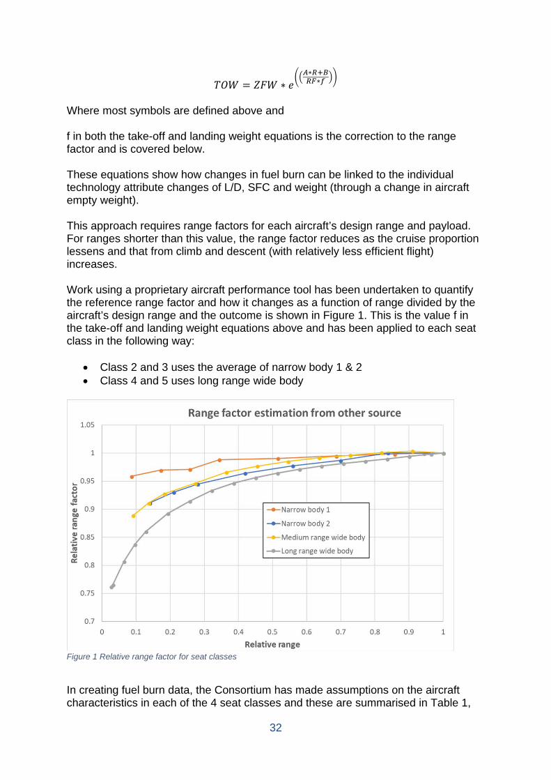
Where most symbols are defined above and f in both the take-off and landing weight equations is the correction to the range factor and is covered below. These equations show how changes in fuel burn can be linked to the individual technology attribute changes of L/D, SFC and weight (through a change in aircraft empty weight). This approach requires range factors for each aircraft’s design range and payload. For ranges shorter than this value, the range factor reduces as the cruise proportion lessens and that from climb and descent (with relatively less efficient flight) increases. Work using a proprietary aircraft performance tool has been undertaken to quantify the reference range factor and how it changes as a function of range divided by the aircraft’s design range and the outcome is shown in Figure 1. This is the value f in the take-off and landing weight equations above and has been applied to each seat class in the following way:

• Class 2 and 3 uses the average of narrow body 1 & 2 • Class 4 and 5 uses long range wide body

Figure 1 Relative range factor for seat classes

In creating fuel burn data, the Consortium has made assumptions on the aircraft characteristics in each of the 4 seat classes and these are summarised in Table 1,

33

where MTOW is the maximum take-off weight and OWE is the operating empty weight. Table 1 Aircraft assumptions for fuel burn data

Seat class Aircraft MTOW (lb) OWE (lb) Payload (lb)

Range factor

2 A319CEO 166,449 93,120 27,720 13,181 3 A320CEO 171,960 95,840 33,600 13,101 4 B777-200ER 656,000 319,700 63,420 16,399 5 B747-400 875,000 398,000 88,620 14,370

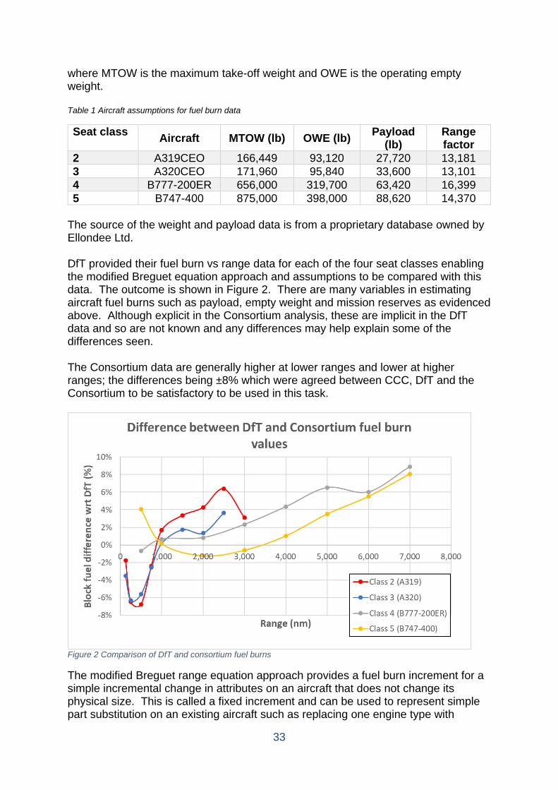
The source of the weight and payload data is from a proprietary database owned by Ellondee Ltd. DfT provided their fuel burn vs range data for each of the four seat classes enabling the modified Breguet equation approach and assumptions to be compared with this data. The outcome is shown in Figure 2. There are many variables in estimating aircraft fuel burns such as payload, empty weight and mission reserves as evidenced above. Although explicit in the Consortium analysis, these are implicit in the DfT data and so are not known and any differences may help explain some of the differences seen. The Consortium data are generally higher at lower ranges and lower at higher ranges; the differences being ±8% which were agreed between CCC, DfT and the Consortium to be satisfactory to be used in this task.

Figure 2 Comparison of DfT and consortium fuel burns

The modified Breguet range equation approach provides a fuel burn increment for a simple incremental change in attributes on an aircraft that does not change its physical size. This is called a fixed increment and can be used to represent simple part substitution on an existing aircraft such as replacing one engine type with

34

another on an unchanged airframe. Improvements in weight, aerodynamic efficiency (L/D) and engine efficiency (specific fuel consumption (SFC)) also offer the potential for the aircraft to change the size of key components such as wing and engine to take advantage of the underlying attribute benefits. This is referred to in this report as a snowballed (also known as rubber) increment and will be larger than the fixed increment. The ratio between snowballed and fixed depends on what is allowed to change and what is kept fixed. For the purposes of this report a 20% increment has been applied to classes 2 and 3 and 30% to classes 4 and 5; these values were chosen based on the Consortium’s previous experience. It must be emphasised that this technique only applies when an aircraft technological change is being proposed.

3.1.4. Results of the assessment This section looks at each of the individual technologies from a weight, aerodynamic efficiency (L/D) and engine efficiency (specific fuel consumption (SFC)) perspective as defined by publicly available information. Where possible, a view on the spread of such attributes has been taken on a worst, nominal and best basis and has been determined by the spread of outcomes from the various reports found in the literature search. Entry into service dates have also been noted where they have been found as well as some commentary on their likely insertion into a new aircraft programme. The Consortium believes that the best individual technologies will be bundled together into new aircraft types, once they are sufficiently mature. Technology developers use a sliding scale of technology maturity; the higher the level the higher the confidence to apply the technology. This report uses the NASA technology readiness level (TRL) definitions (reference [4]) and, based on these definitions sets the minimum level for consideration in an aircraft programme to be at least TRL6. There also needs to be a market opportunity for a new aircraft through either new market development or replacement of older aircraft. This bundling of technologies will be covered in more detail in tasks 2 and 3.

Ultra-High By-pass Ratio Turbofan (UHBR) The rationale behind the UHBR is to achieve a large increase in the amount of air entering the engine rather than going through the core; it by-passes the core down the by-pass duct. The greater the ratio of by-pass to core air, the greater the propulsive efficiency and the lower the SFC. On the negative side it increases engine physical size, weight and drag for a given thrust. For it to reduce fuel burn, the contribution to fuel burn from SFC reduction has to be greater than the increase from the weight and drag increases. Massachusetts Institute of Technology and NASA in references [5] and [6] compare the UBHR performance on an aircraft to replace the 737-800 (very similar timescales and technology to classes 2 and 3). An engine of 20 by-pass ratio (BPR) will reduce fuel burn by 4.2% relative to the baseline [5] whilst [6] suggests a cruise SFC of 0.37 lb/lbf/lhr at 0.74 Mach number in a Boundary Layer Ingestion (BLI) installation with a BPR 20 engine. Later in the report an SFC of 0.43 lb/lbf/hr is quoted and it also shows how SFC varies with Mach number for the same engine suggesting that SFC reduces by 0.01 lb/lbf/hr when Mach number reduces from 0.76 to 0.72. These reports believe that TRL4 will be achieved by 2025 for such an engine.

35

NASA and GE in reference [7] quote a cruise SFC of 0.442 lb/lbf/hr for a similar engine (with a fan diameter of 71 inches) and a dry weight of 6,400 lb but a sea level static thrust of only 22,000 lbf (cf 33,000 lbf for the reference A320 CFM56 engine). Another NASA publication, reference [8], quotes fuel burn savings of 13 to 15% relative to the CFM56-7 (the engine on the 737-800), whilst reference [9] suggests a 28% SFC reduction to a CFM56 (subtype not specified) and a dry weight increase of 1,500lb for an engine with a 77 inch diameter fan and 13 BPR. A round up of SFC and weight changes for UHBR has been included in reference [10], from ICCT, and are summarised in Table 2. In this report the use of EVO (evolutionary), MOD (moderate) and AGG (aggressive) values are taken to have the same broad meaning as worst, nominal and best respectively in this work. Table 2 ICCT SFC and weight improvements for 2034

2034 Reference engine SFC (%) Weight (lb)

EVO MOD AGG EVO MOD AGG Regional jet CF34 -15 -20 -30 -60 -400 -500 Single aisle CFM56 -17 -22 -30 -600 -610 -1,000 Twin aisle GE90 -11 -13 -15 -800 -2,000 -3,500

Fuel burn improvement forecasts can be found in references [11] from ENOVAL and [12] from Rolls-Royce where values of 26% for a long-range engine relative to year 2000 technology and 25% relative to Trent 700 are quoted respectively. Reference [12] also projects a launch for an UHBR in 2025. There is a wealth of information that needs digesting into a consistent set of data for each seat class against their representative technology standards. Reference [13], from Jenkinson and [14] from Rolls-Royce contain engine data that have been used to baseline the reference aircraft. These are shown in Table 3. Table 3 Engine characteristics for DfT reference aircraft

Engine BPR Fan diameter(in)

Dry weight (lb)

Cruise SFC

(lb/lbf/hr)

Reference thrust (lbf)

Class 2 CFM56-5B 5.5 68.3 5,250 0.598 30,000

Class 3 CFM56-5B 5.5 68.3 5,250 0.598 30,000

Class 4 GE90-94B 8.4 123 16,664 0.528 80,000

Class 5 CF6-80C2 5.0 93 9,499 0.564 60,000

A 28% reduction in SFC on the CFM56 from [9] equates to an SFC of 0.43 and this is consistent with [6] and [7]. 22% is the value in [10] and so an aggregate of 25% will be used for the nominal value and 28% for the best value. Other than the ICCT data, there is no easy way to define the worst case as the data are well grouped. It is proposed that the ICCT increment of 5% be taken to represent the worst case.

36

Class 4’s engine is some 12% better on SFC (because of its technology, physical size and BPR) than those in classes 2, 3 and 5. The ICCT data [10] for this class have been set to 13% (probably in recognition of this) and the only other data found in the literature search looks at fuel burn improvement rather than SFC. This equates to the same absolute SFC as the CFM56 and that will not be correct given the benefits that should accrue from physical size. This can be seen in the difference between the CFM56 and CF6-80C2 SFC values (which are similar technology levels and BPR). Application of a 6% increment to the 13% from ICCT (to account for engine size) yields an 18% improvement and this will be used for the nominal value and the same increments used in classes 2 and 3 will be used for the worst and best. Class 5 should achieve the same cruise SFC as class 4 (given similar technology, size and BPR) and that requires a 23% improvement. The same increments used in classes 2 and 3 will be used for the worst and best. Two weight data points have been found for engines in classes 2 and 3. An increment of 1,200 lb can be discerned when comparing the baseline engine with that dry weight quoted in [7] and an increment of 1,500 lb in [9]. The ICCT data in [10] points to weight reductions rather than increases; this is not what recent industry trends of increased BPR have highlighted. The latest technology CFM56 sized engines such as the CFMLeap and the Pratt & Whitney Pure PW1000 series engines are some 1,000 lb heavier than the CFM56 even with the application of the latest weight saving technologies (references [15] [16] and [17], all from EASA apply); the ICCT data are therefore discounted in this report. A nominal weight increment of 1,500 lb per engine is to be used for classes 2 and 3 and a best of 1,200 lb. The worst will take the same increment as between best and nominal. Allowing the same thrust to weight decrease to apply to the classes 4 and 5 will increase weight by 28%. Based on Table 3, class 4 weight per engine will increase by ~5,000 lb and class 5 by ~ 3,000 lb. The same percentage increments will be applied as for classes 2 and 3. There has been no discussion on drag in any of the references found on this topic. A simple analytical assessment approach has been used to assess the change in nacelle drag for the increase in fan diameter required to increase the BPR of the engine; this assumes that nacelle drag change is proportional to diameter2. Any interference drag effects between the nacelle and the rest of the airframe have not been included as industry best practice will seek to remove these through careful aerodynamic tailoring of the local surfaces. For classes 2 and 3, fan diameters of 71 and 77 inches have been declared in [7] and [9] respectively. Taking the 71-inch fan diameter as baseline this equates to a nacelle drag change of 27% for the 77-inch nacelle. A typical cruise drag breakdown by component is shown in [9] and nacelles contribute ~10% to the skin friction drag and skin friction drag contributes ~60% to the total aircraft drag. The resultant drag is around 1.5%. It is unlikely that the drag is going to get any better than this and so the best will be set to the same as the nominal. Under worst conditions, interference drag will not be dealt with and that could be as high as an additional 5% of aircraft drag.

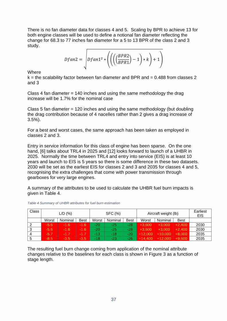
37

There is no fan diameter data for classes 4 and 5. Scaling by BPR to achieve 13 for both engine classes will be used to define a notional fan diameter reflecting the change for 68.3 to 77 inches fan diameter for a 5 to 13 BPR of the class 2 and 3 study.

𝐷𝐷𝑓𝑓𝑟𝑟𝑙𝑙2 = �𝐷𝐷𝑓𝑓𝑟𝑟𝑙𝑙12 ∗ ��𝐵𝐵𝐵𝐵𝑅𝑅2𝐵𝐵𝐵𝐵𝑅𝑅1�

− 1� ∗ 𝑘𝑘� + 1�

Where k = the scalability factor between fan diameter and BPR and = 0.488 from classes 2 and 3 Class 4 fan diameter = 140 inches and using the same methodology the drag increase will be 1.7% for the nominal case Class 5 fan diameter = 120 inches and using the same methodology (but doubling the drag contribution because of 4 nacelles rather than 2 gives a drag increase of 3.5%). For a best and worst cases, the same approach has been taken as employed in classes 2 and 3. Entry in service information for this class of engine has been sparse. On the one hand, [6] talks about TRL4 in 2025 and [12] looks forward to launch of a UHBR in 2025. Normally the time between TRL4 and entry into service (EIS) is at least 10 years and launch to EIS is 5 years so there is some difference in these two datasets. 2030 will be set as the earliest EIS for classes 2 and 3 and 2035 for classes 4 and 5, recognising the extra challenges that come with power transmission through gearboxes for very large engines. A summary of the attributes to be used to calculate the UHBR fuel burn impacts is given in Table 4. Table 4 Summary of UHBR attributes for fuel burn estimation


Worst Nominal Best Worst Nominal Best Worst Nominal Best 2 -5.6 -1.6 -1.6 -20 -25 -28 +3,600 +3,000 +2,400 2030 3 -5.6 -1.6 -1.6 -20 -25 -28 +3,600 +3,000 +2,400 2030 4 -5.7 -1.7 -1.7 -13 -18 -20 +12,000 +10,000 +8,000 2035 5 -8.5 -3.5 -3.5 -18 -23 -26 +14,400 +12,000 +9,600 2035

The resulting fuel burn change coming from application of the nominal attribute changes relative to the baselines for each class is shown in Figure 3 as a function of stage length.

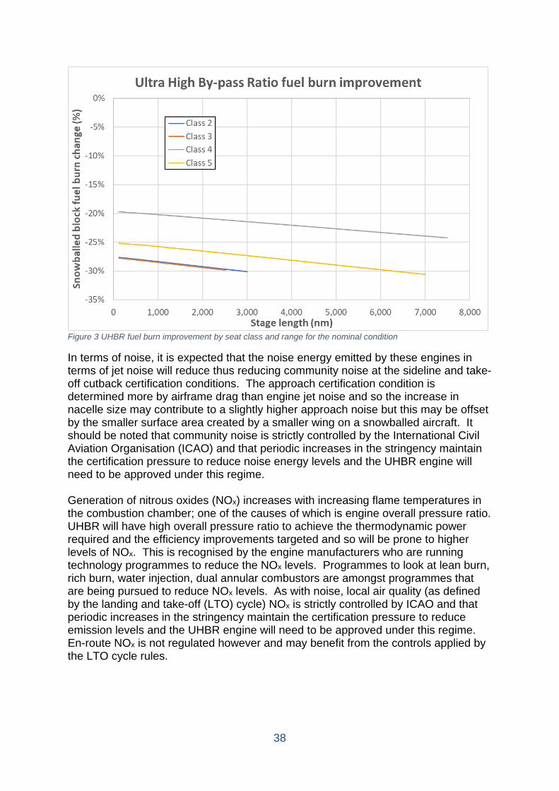
38

Figure 3 UHBR fuel burn improvement by seat class and range for the nominal condition

In terms of noise, it is expected that the noise energy emitted by these engines in terms of jet noise will reduce thus reducing community noise at the sideline and take-off cutback certification conditions. The approach certification condition is determined more by airframe drag than engine jet noise and so the increase in nacelle size may contribute to a slightly higher approach noise but this may be offset by the smaller surface area created by a smaller wing on a snowballed aircraft. It should be noted that community noise is strictly controlled by the International Civil Aviation Organisation (ICAO) and that periodic increases in the stringency maintain the certification pressure to reduce noise energy levels and the UHBR engine will need to be approved under this regime. Generation of nitrous oxides (NOx) increases with increasing flame temperatures in the combustion chamber; one of the causes of which is engine overall pressure ratio. UHBR will have high overall pressure ratio to achieve the thermodynamic power required and the efficiency improvements targeted and so will be prone to higher levels of NOx. This is recognised by the engine manufacturers who are running technology programmes to reduce the NOx levels. Programmes to look at lean burn, rich burn, water injection, dual annular combustors are amongst programmes that are being pursued to reduce NOx levels. As with noise, local air quality (as defined by the landing and take-off (LTO) cycle) NOx is strictly controlled by ICAO and that periodic increases in the stringency maintain the certification pressure to reduce emission levels and the UHBR engine will need to be approved under this regime. En-route NOx is not regulated however and may benefit from the controls applied by the LTO cycle rules.

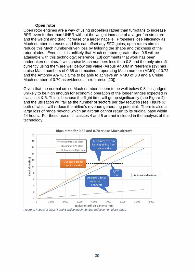
39

Open rotor Open rotor engines are a way of using propellers rather than turbofans to increase BPR even further than UHBR without the weight increase of a larger fan structure and the weight and drag increase of a larger nacelle. Propellers lose efficiency as Mach number increases and this can offset any SFC gains; open rotors aim to reduce this Mach number-driven loss by tailoring the shape and thickness of the rotor blades. Even so, it is unlikely that Mach numbers greater than 0.8 will be attainable with this technology; reference [18] comments that work has been undertaken on aircraft with cruise Mach numbers less than 0.8 and the only aircraft currently using them are well below this value (Airbus A400M in reference [19] has cruise Mach numbers of 0.68 and maximum operating Mach number (MMO) of 0.72 and the Antonov An-70 claims to be able to achieve an MMO of 0.8 and a Cruise Mach number of 0.70 as evidenced in reference [20]). Given that the normal cruise Mach numbers seem to be well below 0.8, it is judged unlikely to be high enough for economic operation of the longer ranges expected in classes 4 & 5. This is because the flight time will go up significantly (see Figure 4) and the utilisation will fall as the number of sectors per day reduces (see Figure 5); both of which will reduce the airline’s revenue generating potential. There is also a large loss of range beyond which an aircraft cannot return to its original base within 24 hours. For these reasons, classes 4 and 5 are not included in the analysis of this technology.

Figure 4: Impact of class 4 and 5 cruise Mach number reduction on block times

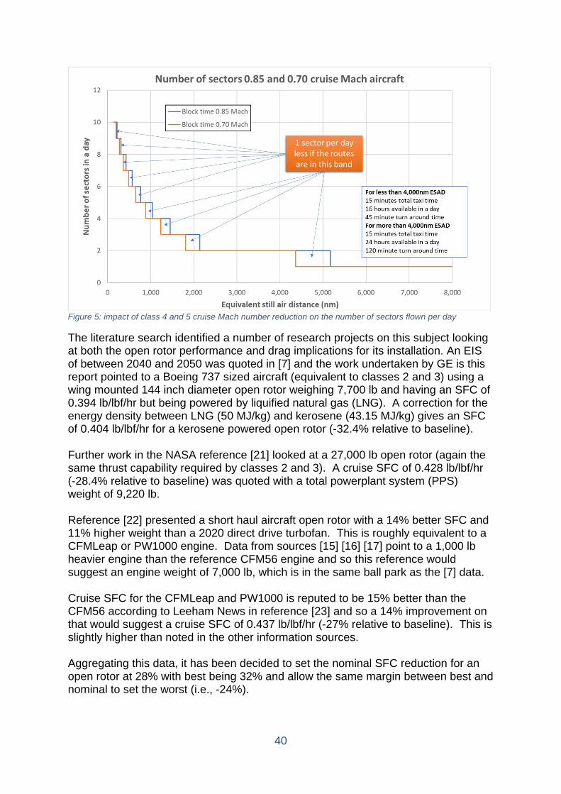
40

Figure 5: impact of class 4 and 5 cruise Mach number reduction on the number of sectors flown per day

The literature search identified a number of research projects on this subject looking at both the open rotor performance and drag implications for its installation. An EIS of between 2040 and 2050 was quoted in [7] and the work undertaken by GE is this report pointed to a Boeing 737 sized aircraft (equivalent to classes 2 and 3) using a wing mounted 144 inch diameter open rotor weighing 7,700 lb and having an SFC of 0.394 lb/lbf/hr but being powered by liquified natural gas (LNG). A correction for the energy density between LNG (50 MJ/kg) and kerosene (43.15 MJ/kg) gives an SFC of 0.404 lb/lbf/hr for a kerosene powered open rotor (-32.4% relative to baseline). Further work in the NASA reference [21] looked at a 27,000 lb open rotor (again the same thrust capability required by classes 2 and 3). A cruise SFC of 0.428 lb/lbf/hr (-28.4% relative to baseline) was quoted with a total powerplant system (PPS) weight of 9,220 lb. Reference [22] presented a short haul aircraft open rotor with a 14% better SFC and 11% higher weight than a 2020 direct drive turbofan. This is roughly equivalent to a CFMLeap or PW1000 engine. Data from sources [15] [16] [17] point to a 1,000 lb heavier engine than the reference CFM56 engine and so this reference would suggest an engine weight of 7,000 lb, which is in the same ball park as the [7] data. Cruise SFC for the CFMLeap and PW1000 is reputed to be 15% better than the CFM56 according to Leeham News in reference [23] and so a 14% improvement on that would suggest a cruise SFC of 0.437 lb/lbf/hr (-27% relative to baseline). This is slightly higher than noted in the other information sources. Aggregating this data, it has been decided to set the nominal SFC reduction for an open rotor at 28% with best being 32% and allow the same margin between best and nominal to set the worst (i.e., -24%).

41

The only source on aircraft drag due to open rotors was found in reference [24] and looked at both fuselage and wing mounted open rotors. Based on computational fluid dynamic (CFD) assessments the wing mounted installation increased drag by 3% whereas the fuselage mounted installation reduced drag by about 0.5%. From a drag perspective there is only one data point that suggests wing mounted engines will have a drag increase of 3% and rear fuselage mounted as 0.5%. These will be used to set nominal and best. As with UHBR an additional 5% will be added to nominal to allow for the worst possible interference drag standard. Where the weight is declared as a dry engine weight, the increment is around 1,500 lb giving a total increment of around 2,500 lb when corrected for the year 2020 technology baseline point. The higher weight of 9,220 lb is a PPS weight and will include accessories and other installation fitments so is not directly comparable with the dry engine weight. Massachusetts Institute of Technology reference [25] suggests that these items contribute about 18% to a PPS and so this allows a simple correction to be made to get a rough dry engine weight estimate of ~7,600 lb. This is remarkably close to the other data point. The nominal weight increase per engine has thus been set at 2,500 lb based on this data with a margin of best and worst set at 1,800 lb and 3,200 lb. EIS is only referenced in one document and points to between 2040 and 2050. It is known that Safran have been running an open rotor demonstration programme as part of EU research programme CleanSky2 and that there are no active programmes in the US. Whilst the original intent was to fly the engine on the CleanSky2 project, it is understood that this has been downgraded to a series of ground tests, possibly suggesting that the impetus to develop this technology within Europe has reduced. This is consistent with a late entry into service although it is possible that rapid and large increases in fuel price may re-energise the interest in the technology. It is proposed that 2040 be set as the EIS. Table 5 Summary of Open Rotor attributes for fuel burn estimation


Worst Nominal Best Worst Nominal Best Worst Nominal Best 2 -5% -3% -0.5% -24 -28 -32 +6,400 +5,000 +3,600 2040 3 -5% -3% -0.5% -24 -28 -32 +6,400 +5,000 +3,600 2040

The resulting fuel burn change coming from application of the nominal attribute changes relative to the baselines for each class and stage length is shown in Figure 6.

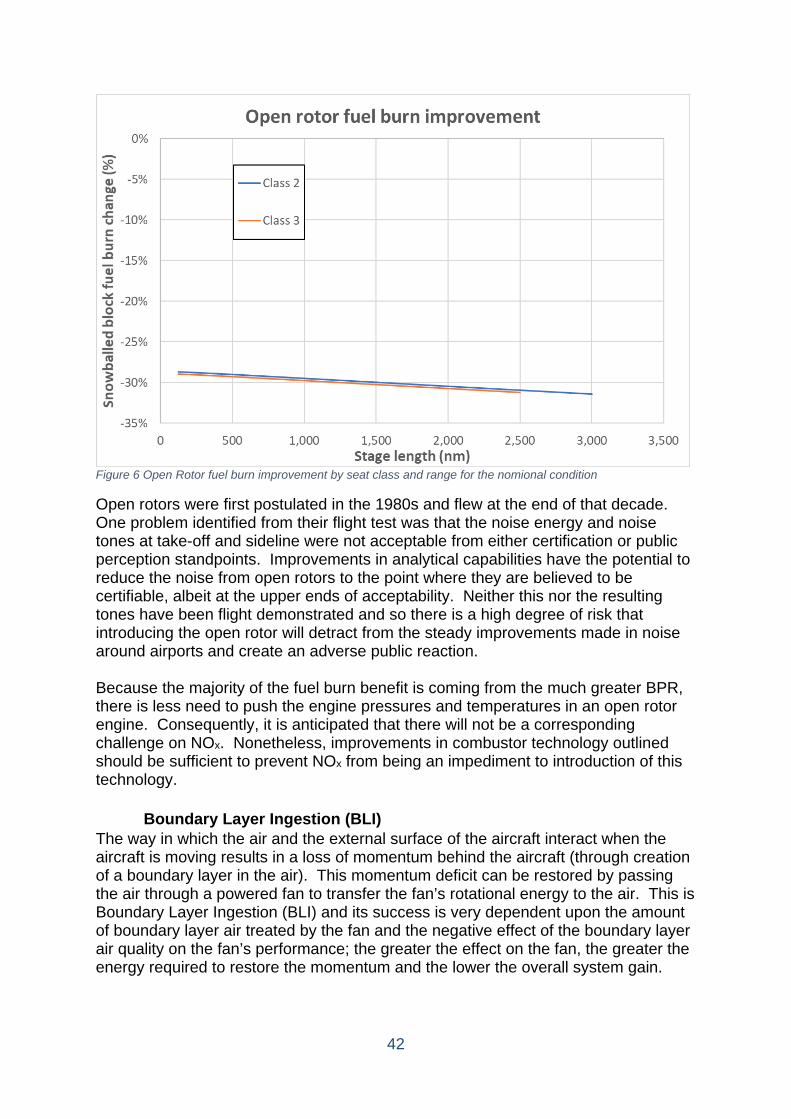
42

Figure 6 Open Rotor fuel burn improvement by seat class and range for the nomional condition

Open rotors were first postulated in the 1980s and flew at the end of that decade. One problem identified from their flight test was that the noise energy and noise tones at take-off and sideline were not acceptable from either certification or public perception standpoints. Improvements in analytical capabilities have the potential to reduce the noise from open rotors to the point where they are believed to be certifiable, albeit at the upper ends of acceptability. Neither this nor the resulting tones have been flight demonstrated and so there is a high degree of risk that introducing the open rotor will detract from the steady improvements made in noise around airports and create an adverse public reaction. Because the majority of the fuel burn benefit is coming from the much greater BPR, there is less need to push the engine pressures and temperatures in an open rotor engine. Consequently, it is anticipated that there will not be a corresponding challenge on NOx. Nonetheless, improvements in combustor technology outlined should be sufficient to prevent NOx from being an impediment to introduction of this technology.

Boundary Layer Ingestion (BLI) The way in which the air and the external surface of the aircraft interact when the aircraft is moving results in a loss of momentum behind the aircraft (through creation of a boundary layer in the air). This momentum deficit can be restored by passing the air through a powered fan to transfer the fan’s rotational energy to the air. This is Boundary Layer Ingestion (BLI) and its success is very dependent upon the amount of boundary layer air treated by the fan and the negative effect of the boundary layer air quality on the fan’s performance; the greater the effect on the fan, the greater the energy required to restore the momentum and the lower the overall system gain.

43

As the drag reduces there is the potential to reduce the size of the main engines thereby reducing overall weight and drag to compensate for the increase in weight and drag for the BLI propulsor. This topic has been of great interest to researchers in recent times and reference [5] thought that BLI would get to TRL 4 by 2025. Other reports focus on overall fuel burn benefits and show a large variation in outcomes such as [6] (9.5%),and NASA studies in references [26] (up to 16%) and [27] (~10%), reference [28] (3.8%), and Pittsburgh University reference [29] (5 to 10%). Only two reports sought to look at weight, drag and SFC contributions to the BLI fuel burn improvement. A 9% fuel burn reduction was claimed in a NASA reference [30] made up of a 6% drag reduction, 4,500 lb weight reduction but a 4% SFC increase on a 450-seater blended wing body (BWB) aircraft (similar to class 5). A 5% fuel burn saving is claimed in another NASA reference [31], also for a BWB. A 2% drag improvement is postulated along with a 6,000 lb weight reduction and a 2% SFC increase. There is no reported data for classes 2 and 3. SFC will increase because of the effect of ingesting the boundary layer and its negative impact on fan performance. Only two reports quote values of between 2 and 4% increase and this is very dependent on the integration of fuselage and intake, the degree of the boundary layer swallowed and the design of the fan to balance performance and integrity. It is proposed to use the higher value of SFC loss (4%) as nominal (for all classes) the integration challenges are not yet well understood and the 2% as best. It is also noted that these are both for engines mounted on the upper surface of a BWB and not on the rear fuselage of a conventional layout; the BWB layout may provide easier intake conditions for the intake during most flight phases as the air flow is largely two dimensional, unlike a cylindrical fuselage that is always three dimensional, especially in the presence of any upsweep. Worst could be almost any value given the potential mechanical and aerodynamic impact of boundary layer air on fan performance and will be driven the need to gain an overall system advantage if the technology is to be adopted. This report will arbitrarily set the worst case at 10% loss of SFC. Weight information has only been provided from two data points and both on BWB-450 and this is driven mainly by reduced engine sizes because of the lower overall aircraft drag. Take-off weight for this aircraft is quoted at ~ 800,000 lb with three engines. Taking a simple all engines operating take-off thrust to weight ratio for take-off of 0.3 (industry standard) then the engine size for the reported BWB will be ~80,000 lb each. In simple terms, engine weight is proportional to an “engine linear dimension” cubed and thrust is proportional to “engine linear dimension” squared. Incremental engine weight can therefore be simply scaled by thrust to the power of 1.5. Engines for classes 2 and 3 are in the 30,000 lb thrust class and so the 2,000 lb reduction in per engine weight (6,000l b over three engines on the BWB) translates into 500 lb/engine for these smaller aircraft classes. Similarly, the weight increment for the 90,000 lb thrust engines of class 4 becomes 2,400 lb/engine and the 60,000 lb thrust class on the four-engine class 5 becomes 1,300 lb/engine. At an aircraft

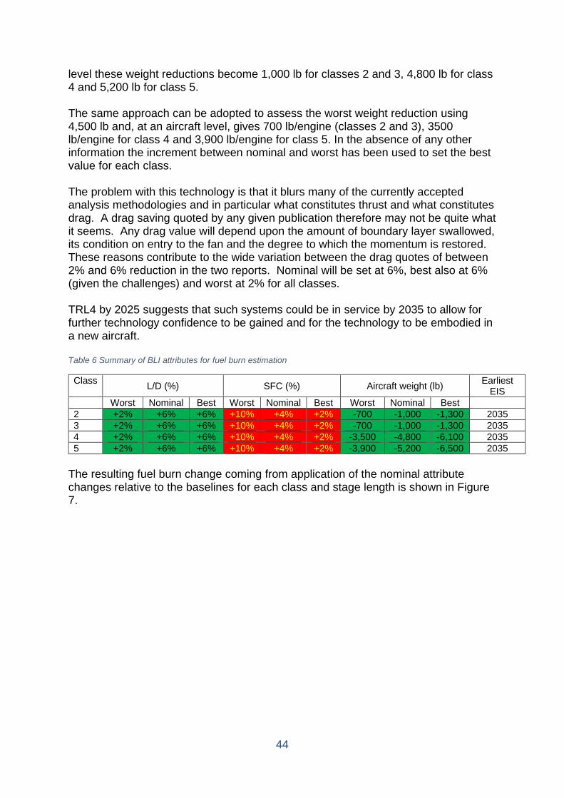
44

level these weight reductions become 1,000 lb for classes 2 and 3, 4,800 lb for class 4 and 5,200 lb for class 5. The same approach can be adopted to assess the worst weight reduction using 4,500 lb and, at an aircraft level, gives 700 lb/engine (classes 2 and 3), 3500 lb/engine for class 4 and 3,900 lb/engine for class 5. In the absence of any other information the increment between nominal and worst has been used to set the best value for each class. The problem with this technology is that it blurs many of the currently accepted analysis methodologies and in particular what constitutes thrust and what constitutes drag. A drag saving quoted by any given publication therefore may not be quite what it seems. Any drag value will depend upon the amount of boundary layer swallowed, its condition on entry to the fan and the degree to which the momentum is restored. These reasons contribute to the wide variation between the drag quotes of between 2% and 6% reduction in the two reports. Nominal will be set at 6%, best also at 6% (given the challenges) and worst at 2% for all classes. TRL4 by 2025 suggests that such systems could be in service by 2035 to allow for further technology confidence to be gained and for the technology to be embodied in a new aircraft. Table 6 Summary of BLI attributes for fuel burn estimation


Worst Nominal Best Worst Nominal Best Worst Nominal Best 2 +2% +6% +6% +10% +4% +2% -700 -1,000 -1,300 2035 3 +2% +6% +6% +10% +4% +2% -700 -1,000 -1,300 2035 4 +2% +6% +6% +10% +4% +2% -3,500 -4,800 -6,100 2035 5 +2% +6% +6% +10% +4% +2% -3,900 -5,200 -6,500 2035


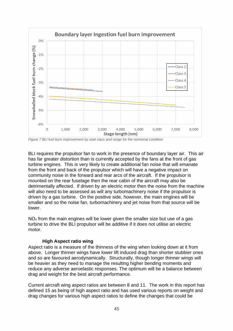
45

Figure 7 BLI fuel burn improvement by seat class and range for the nomional condition

BLI requires the propulsor fan to work in the presence of boundary layer air. This air has far greater distortion than is currently accepted by the fans at the front of gas turbine engines. This is very likely to create additional fan noise that will emanate from the front and back of the propulsor which will have a negative impact on community noise in the forward and rear arcs of the aircraft. If the propulsor is mounted on the rear fuselage then the rear cabin of the aircraft may also be detrimentally affected. If driven by an electric motor then the noise from the machine will also need to be assessed as will any turbomachinery noise if the propulsor is driven by a gas turbine. On the positive side, however, the main engines will be smaller and so the noise fan, turbomachinery and jet noise from that source will be lower. NOx from the main engines will be lower given the smaller size but use of a gas turbine to drive the BLI propulsor will be additive if it does not utilise an electric motor.

High Aspect ratio wing Aspect ratio is a measure of the thinness of the wing when looking down at it from above. Longer thinner wings have lower lift induced drag than shorter stubbier ones and so are favoured aerodynamically. Structurally, though longer thinner wings will be heavier as they need to manage the resulting higher bending moments and reduce any adverse aeroelastic responses. The optimum will be a balance between drag and weight for the best aircraft performance. Current aircraft wing aspect ratios are between 8 and 11. The work in this report has defined 15 as being of high aspect ratio and has used various reports on weight and drag changes for various high aspect ratios to define the changes that could be

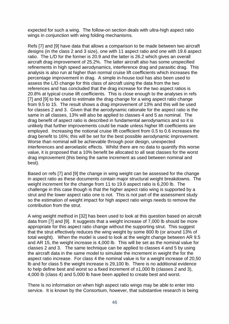
46

expected for such a wing. The follow-on section deals with ultra-high aspect ratio wings in conjunction with wing folding mechanisms. Refs [7] and [9] have data that allows a comparison to be made between two aircraft designs (in the class 2 and 3 size), one with 11 aspect ratio and one with 19.6 aspect ratio. The L/D for the former is 20.9 and the latter is 26.2 which gives an overall aircraft drag improvement of 25.2%. The latter aircraft also has some unspecified refinements in high speed aerodynamics, interference drag and parasitic drag. This analysis is also run at higher than normal cruise lift coefficients which increases the percentage improvement in drag. A simple in-house tool has also been used to assess the L/D change for this class of aircraft using the data from the two references and has concluded that the drag increase for the two aspect ratios is 20.8% at typical cruise lift coefficients. This is close enough to the analyses in refs [7] and [9] to be used to estimate the drag change for a wing aspect ratio change from 9.5 to 15. The result shows a drag improvement of 13% and this will be used for classes 2 and 3. Given that the aerodynamic rationale for the aspect ratio is the same in all classes, 13% will also be applied to classes 4 and 5 as nominal. The drag benefit of aspect ratio is described in fundamental aerodynamics and so it is unlikely that further improvements could be made unless higher lift coefficients are employed. Increasing the notional cruise lift coefficient from 0.5 to 0.6 increases the drag benefit to 16%; this will be set for the best possible aerodynamic improvement. Worse than nominal will be achievable through poor design, unexpected interferences and aeroelastic effects. Whilst there are no data to quantify this worse value, it is proposed that a 10% benefit be allocated to all seat classes for the worst drag improvement (this being the same increment as used between nominal and best). Based on refs [7] and [9] the change in wing weight can be assessed for the change in aspect ratio as these documents contain major structural weight breakdowns. The weight increment for the change from 11 to 19.6 aspect ratio is 6,200 lb. The challenge in this case though is that the higher aspect ratio wing is supported by a strut and the lower aspect ratio one is not. This is not part of the assessment study so the estimation of weight impact for high aspect ratio wings needs to remove the contribution from the strut. A wing weight method in [32] has been used to look at this question based on aircraft data from [7] and [9]. It suggests that a weight increase of 7,000 lb should be more appropriate for this aspect ratio change without the supporting strut. This suggest that the strut effectively reduces the wing weight by some 800 lb (or around 13% of total weight). When the model is used to look at the weight change between AR 9.5 and AR 15, the weight increase is 4,000 lb. This will be set as the nominal value for classes 2 and 3. The same technique can be applied to classes 4 and 5 by using the aircraft data in the same model to simulate the increment in weight the for the aspect ratio increase. For class 4 the nominal value is for a weight increase of 20,50 lb and for class 5 the weight increase is 29,100 lb. There is no additional evidence to help define best and worst so a fixed increment of ±1,000 lb (classes 2 and 3), 4,000 lb (class 4) and 5,000 lb have been applied to create best and worst. There is no information on when high aspect ratio wings may be able to enter into service. It is known by the Consortium, however, that substantive research is being

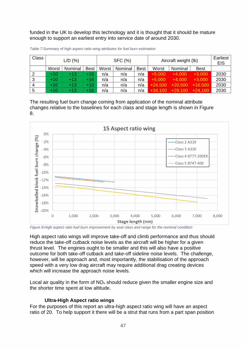
47

funded in the UK to develop this technology and it is thought that it should be mature enough to support an earliest entry into service date of around 2030. Table 7:Summary of high aspect ratio wing attributes for fuel burn estimation


Worst Nominal Best Worst Nominal Best Worst Nominal Best 2 +10 +13 +16 n/a n/a n/a +5,000 +4,000 +3,000 2030 3 +10 +13 +16 n/a n/a n/a +5,000 +4,000 +3,000 2030 4 +10 +13 +16 n/a n/a n/a +24,500 +20,500 +16,500 2030 5 +10 +13 +16 n/a n/a n/a +34,100 +29,100 +24,100 2030


Figure 8:High aspect ratio fuel burn improvement by seat class and range for the nominal condition

High aspect ratio wings will improve take-off and climb performance and thus should reduce the take-off cutback noise levels as the aircraft will be higher for a given thrust level. The engines ought to be smaller and this will also have a positive outcome for both take-off cutback and take-off sideline noise levels. The challenge, however, will be approach and, most importantly, the stabilisation of the approach speed with a very low drag aircraft may require additional drag creating devices which will increase the approach noise levels. Local air quality in the form of NOx should reduce given the smaller engine size and the shorter time spent at low altitude.

Ultra-High Aspect ratio wings For the purposes of this report an ultra-high aspect ratio wing will have an aspect ratio of 20. To help support it there will be a strut that runs from a part span position

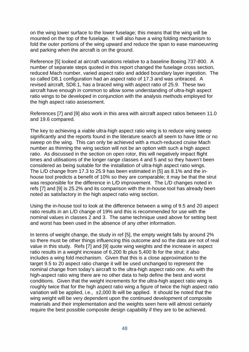
48

on the wing lower surface to the lower fuselage; this means that the wing will be mounted on the top of the fuselage. It will also have a wing folding mechanism to fold the outer portions of the wing upward and reduce the span to ease manoeuvring and parking when the aircraft is on the ground. Reference [5] looked at aircraft variations relative to a baseline Boeing 737-800. A number of separate steps quoted in this report changed the fuselage cross section, reduced Mach number, varied aspect ratio and added boundary layer ingestion. The so called D8.1 configuration had an aspect ratio of 17.3 and was unbraced. A revised aircraft, SD8.1, has a braced wing with aspect ratio of 25.9. These two aircraft have enough in common to allow some understanding of ultra-high aspect ratio wings to be developed in conjunction with the analysis methods employed for the high aspect ratio assessment. References [7] and [9] also work in this area with aircraft aspect ratios between 11.0 and 19.6 compared. The key to achieving a viable ultra-high aspect ratio wing is to reduce wing sweep significantly and the reports found in the literature search all seem to have little or no sweep on the wing. This can only be achieved with a much-reduced cruise Mach number as thinning the wing section will not be an option with such a high aspect ratio. As discussed in the section on open rotor, this will negatively impact flight times and utilisations of the longer range classes 4 and 5 and so they haven’t been considered as being suitable for the installation of ultra-high aspect ratio wings. The L/D change from 17.3 to 25.9 has been estimated in [5] as 8.1% and the in-house tool predicts a benefit of 10% so they are comparable; it may be that the strut was responsible for the difference in L/D improvement. The L/D changes noted in refs [7] and [9] is 25.2% and its comparison with the in-house tool has already been noted as satisfactory in the high aspect ratio wing section. Using the in-house tool to look at the difference between a wing of 9.5 and 20 aspect ratio results in an L/D change of 19% and this is recommended for use with the nominal values in classes 2 and 3. The same technique used above for setting best and worst has been used in the absence of any other information. In terms of weight change, the study in ref [5], the empty weight falls by around 2% so there must be other things influencing this outcome and so the data are not of real value in this study. Refs [7] and [9] quote wing weights and the increase in aspect ratio results in a weight increase of 6,200 lb plus 5,400 lb for the strut; it also includes a wing fold mechanism. Given that this is a close approximation to the target 9.5 to 20 aspect ratio change it will be used unchanged to represent the nominal change from today’s aircraft to the ultra-high aspect ratio one. As with the high-aspect ratio wing there are no other data to help define the best and worst conditions. Given that the weight increments for the ultra-high aspect ratio wing is roughly twice that for the high aspect ratio wing a figure of twice the high aspect ratio variation will be applied, i.e., ±2,000 lb will be applied. It should be noted that the wing weight will be very dependent upon the continued development of composite materials and their implementation and the weights seen here will almost certainly require the best possible composite design capability if they are to be achieved.

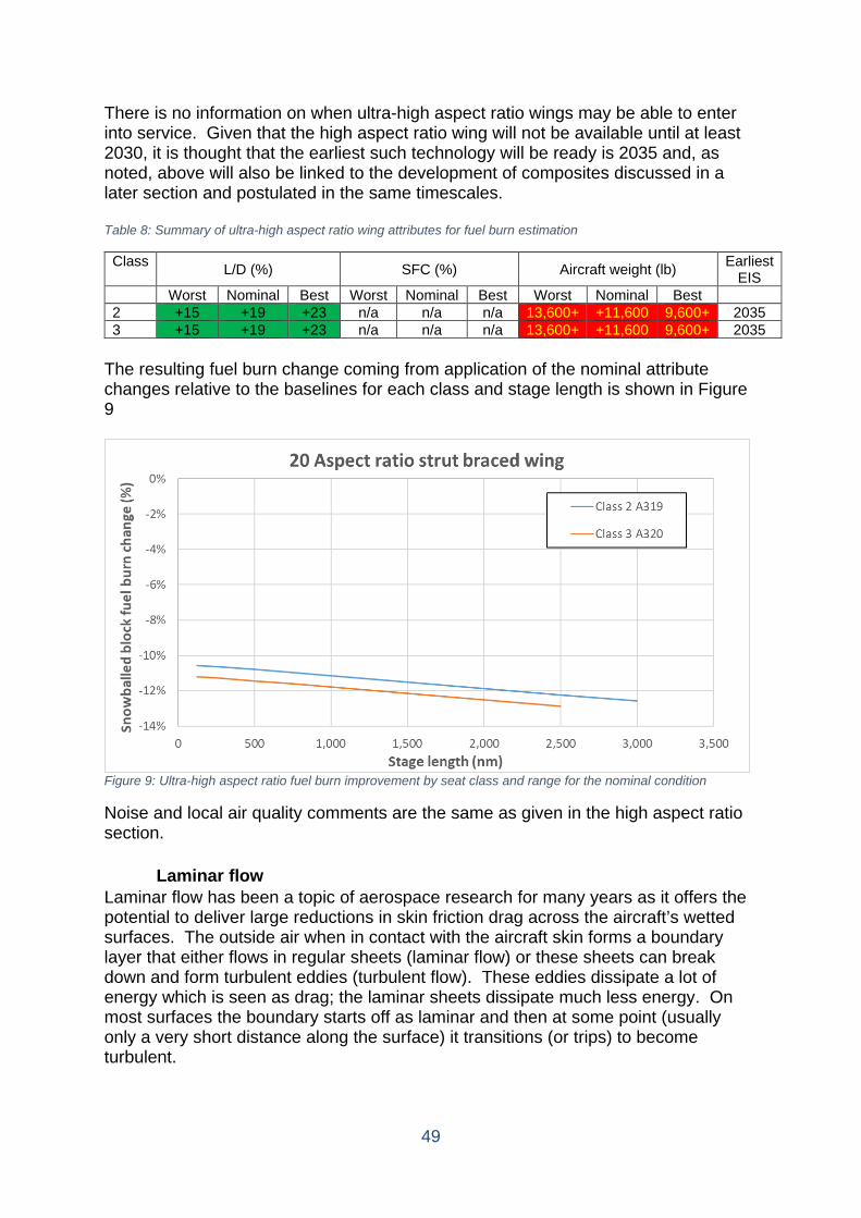
49

There is no information on when ultra-high aspect ratio wings may be able to enter into service. Given that the high aspect ratio wing will not be available until at least 2030, it is thought that the earliest such technology will be ready is 2035 and, as noted, above will also be linked to the development of composites discussed in a later section and postulated in the same timescales. Table 8: Summary of ultra-high aspect ratio wing attributes for fuel burn estimation


Worst Nominal Best Worst Nominal Best Worst Nominal Best 2 +15 +19 +23 n/a n/a n/a 13,600+ +11,600 9,600+ 2035 3 +15 +19 +23 n/a n/a n/a 13,600+ +11,600 9,600+ 2035

The resulting fuel burn change coming from application of the nominal attribute changes relative to the baselines for each class and stage length is shown in Figure 9

Figure 9: Ultra-high aspect ratio fuel burn improvement by seat class and range for the nominal condition

Noise and local air quality comments are the same as given in the high aspect ratio section.

Laminar flow Laminar flow has been a topic of aerospace research for many years as it offers the potential to deliver large reductions in skin friction drag across the aircraft’s wetted surfaces. The outside air when in contact with the aircraft skin forms a boundary layer that either flows in regular sheets (laminar flow) or these sheets can break down and form turbulent eddies (turbulent flow). These eddies dissipate a lot of energy which is seen as drag; the laminar sheets dissipate much less energy. On most surfaces the boundary starts off as laminar and then at some point (usually only a very short distance along the surface) it transitions (or trips) to become turbulent.

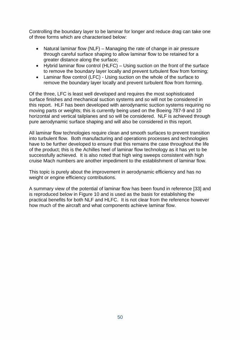
50

Controlling the boundary layer to be laminar for longer and reduce drag can take one of three forms which are characterised below:

• Natural laminar flow (NLF) – Managing the rate of change in air pressure through careful surface shaping to allow laminar flow to be retained for a greater distance along the surface;

• Hybrid laminar flow control (HLFC) – Using suction on the front of the surface to remove the boundary layer locally and prevent turbulent flow from forming;

• Laminar flow control (LFC) - Using suction on the whole of the surface to remove the boundary layer locally and prevent turbulent flow from forming.

Of the three, LFC is least well developed and requires the most sophisticated surface finishes and mechanical suction systems and so will not be considered in this report. HLF has been developed with aerodynamic suction systems requiring no moving parts or weights; this is currently being used on the Boeing 787-9 and 10 horizontal and vertical tailplanes and so will be considered. NLF is achieved through pure aerodynamic surface shaping and will also be considered in this report. All laminar flow technologies require clean and smooth surfaces to prevent transition into turbulent flow. Both manufacturing and operations processes and technologies have to be further developed to ensure that this remains the case throughout the life of the product; this is the Achilles heel of laminar flow technology as it has yet to be successfully achieved. It is also noted that high wing sweeps consistent with high cruise Mach numbers are another impediment to the establishment of laminar flow. This topic is purely about the improvement in aerodynamic efficiency and has no weight or engine efficiency contributions. A summary view of the potential of laminar flow has been found in reference [33] and is reproduced below in Figure 10 and is used as the basis for establishing the practical benefits for both NLF and HLFC. It is not clear from the reference however how much of the aircraft and what components achieve laminar flow.

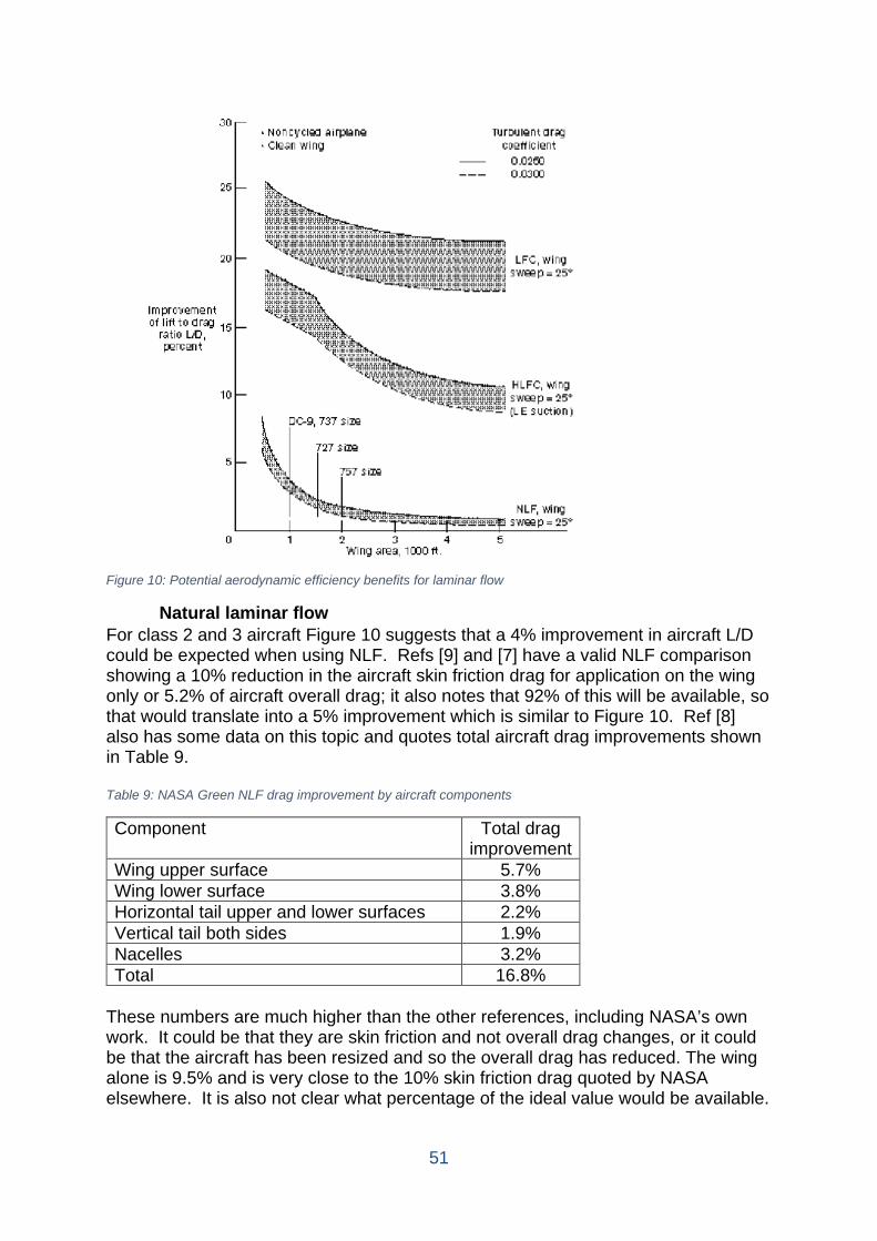
51

Figure 10: Potential aerodynamic efficiency benefits for laminar flow

Natural laminar flow For class 2 and 3 aircraft Figure 10 suggests that a 4% improvement in aircraft L/D could be expected when using NLF. Refs [9] and [7] have a valid NLF comparison showing a 10% reduction in the aircraft skin friction drag for application on the wing only or 5.2% of aircraft overall drag; it also notes that 92% of this will be available, so that would translate into a 5% improvement which is similar to Figure 10. Ref [8] also has some data on this topic and quotes total aircraft drag improvements shown in Table 9. Table 9: NASA Green NLF drag improvement by aircraft components

Component Total drag improvement

Wing upper surface 5.7% Wing lower surface 3.8% Horizontal tail upper and lower surfaces 2.2% Vertical tail both sides 1.9% Nacelles 3.2% Total 16.8%

These numbers are much higher than the other references, including NASA’s own work. It could be that they are skin friction and not overall drag changes, or it could be that the aircraft has been resized and so the overall drag has reduced. The wing alone is 9.5% and is very close to the 10% skin friction drag quoted by NASA elsewhere. It is also not clear what percentage of the ideal value would be available.

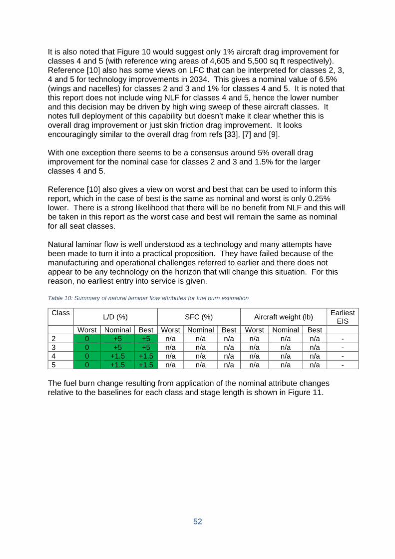
52

It is also noted that Figure 10 would suggest only 1% aircraft drag improvement for classes 4 and 5 (with reference wing areas of 4,605 and 5,500 sq ft respectively). Reference [10] also has some views on LFC that can be interpreted for classes 2, 3, 4 and 5 for technology improvements in 2034. This gives a nominal value of 6.5% (wings and nacelles) for classes 2 and 3 and 1% for classes 4 and 5. It is noted that this report does not include wing NLF for classes 4 and 5, hence the lower number and this decision may be driven by high wing sweep of these aircraft classes. It notes full deployment of this capability but doesn’t make it clear whether this is overall drag improvement or just skin friction drag improvement. It looks encouragingly similar to the overall drag from refs [33], [7] and [9]. With one exception there seems to be a consensus around 5% overall drag improvement for the nominal case for classes 2 and 3 and 1.5% for the larger classes 4 and 5. Reference [10] also gives a view on worst and best that can be used to inform this report, which in the case of best is the same as nominal and worst is only 0.25% lower. There is a strong likelihood that there will be no benefit from NLF and this will be taken in this report as the worst case and best will remain the same as nominal for all seat classes. Natural laminar flow is well understood as a technology and many attempts have been made to turn it into a practical proposition. They have failed because of the manufacturing and operational challenges referred to earlier and there does not appear to be any technology on the horizon that will change this situation. For this reason, no earliest entry into service is given. Table 10: Summary of natural laminar flow attributes for fuel burn estimation


Worst Nominal Best Worst Nominal Best Worst Nominal Best 2 0 +5 +5 n/a n/a n/a n/a n/a n/a - 3 0 +5 +5 n/a n/a n/a n/a n/a n/a - 4 0 +1.5 +1.5 n/a n/a n/a n/a n/a n/a - 5 0 +1.5 +1.5 n/a n/a n/a n/a n/a n/a -

The fuel burn change resulting from application of the nominal attribute changes relative to the baselines for each class and stage length is shown in Figure 11.

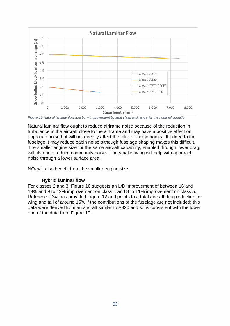
53

Figure 11:Natural laminar flow fuel burn improvement by seat class and range for the nominal condition

Natural laminar flow ought to reduce airframe noise because of the reduction in turbulence in the aircraft close to the airframe and may have a positive effect on approach noise but will not directly affect the take-off noise points. If added to the fuselage it may reduce cabin noise although fuselage shaping makes this difficult. The smaller engine size for the same aircraft capability, enabled through lower drag, will also help reduce community noise. The smaller wing will help with approach noise through a lower surface area. NOx will also benefit from the smaller engine size.

Hybrid laminar flow For classes 2 and 3, Figure 10 suggests an L/D improvement of between 16 and 19% and 9 to 12% improvement on class 4 and 8 to 11% improvement on class 5. Reference [34] has provided Figure 12 and points to a total aircraft drag reduction for wing and tail of around 15% if the contributions of the fuselage are not included; this data were derived from an aircraft similar to A320 and so is consistent with the lower end of the data from Figure 10.

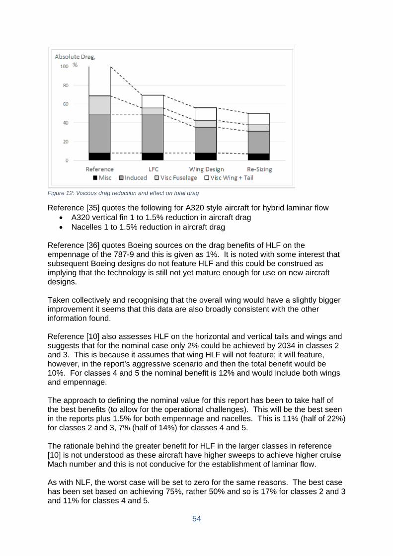
54

Figure 12: Viscous drag reduction and effect on total drag

Reference [35] quotes the following for A320 style aircraft for hybrid laminar flow • A320 vertical fin 1 to 1.5% reduction in aircraft drag • Nacelles 1 to 1.5% reduction in aircraft drag

Reference [36] quotes Boeing sources on the drag benefits of HLF on the empennage of the 787-9 and this is given as 1%. It is noted with some interest that subsequent Boeing designs do not feature HLF and this could be construed as implying that the technology is still not yet mature enough for use on new aircraft designs. Taken collectively and recognising that the overall wing would have a slightly bigger improvement it seems that this data are also broadly consistent with the other information found. Reference [10] also assesses HLF on the horizontal and vertical tails and wings and suggests that for the nominal case only 2% could be achieved by 2034 in classes 2 and 3. This is because it assumes that wing HLF will not feature; it will feature, however, in the report’s aggressive scenario and then the total benefit would be 10%. For classes 4 and 5 the nominal benefit is 12% and would include both wings and empennage. The approach to defining the nominal value for this report has been to take half of the best benefits (to allow for the operational challenges). This will be the best seen in the reports plus 1.5% for both empennage and nacelles. This is 11% (half of 22%) for classes 2 and 3, 7% (half of 14%) for classes 4 and 5. The rationale behind the greater benefit for HLF in the larger classes in reference [10] is not understood as these aircraft have higher sweeps to achieve higher cruise Mach number and this is not conducive for the establishment of laminar flow. As with NLF, the worst case will be set to zero for the same reasons. The best case has been set based on achieving 75%, rather 50% and so is 17% for classes 2 and 3 and 11% for classes 4 and 5.

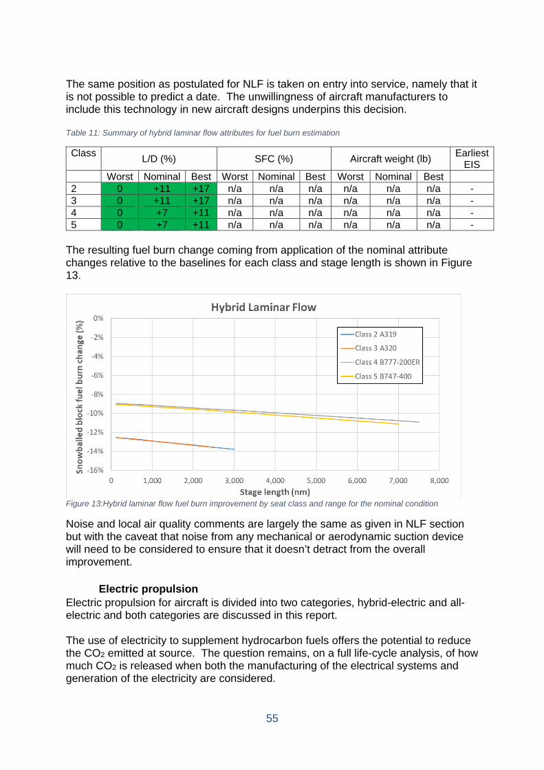
55

The same position as postulated for NLF is taken on entry into service, namely that it is not possible to predict a date. The unwillingness of aircraft manufacturers to include this technology in new aircraft designs underpins this decision. Table 11: Summary of hybrid laminar flow attributes for fuel burn estimation


Worst Nominal Best Worst Nominal Best Worst Nominal Best 2 0 +11 +17 n/a n/a n/a n/a n/a n/a - 3 0 +11 +17 n/a n/a n/a n/a n/a n/a - 4 0 +7 +11 n/a n/a n/a n/a n/a n/a - 5 0 +7 +11 n/a n/a n/a n/a n/a n/a -


Figure 13:Hybrid laminar flow fuel burn improvement by seat class and range for the nominal condition

Noise and local air quality comments are largely the same as given in NLF section but with the caveat that noise from any mechanical or aerodynamic suction device will need to be considered to ensure that it doesn’t detract from the overall improvement.

Electric propulsion Electric propulsion for aircraft is divided into two categories, hybrid-electric and all-electric and both categories are discussed in this report. The use of electricity to supplement hydrocarbon fuels offers the potential to reduce the CO2 emitted at source. The question remains, on a full life-cycle analysis, of how much CO2 is released when both the manufacturing of the electrical systems and generation of the electricity are considered.

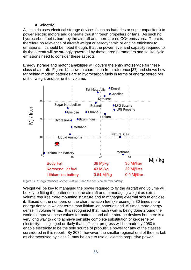
56

All-electric All electric uses electrical storage devices (such as batteries or super capacitors) to power electric motors and generate thrust through propellers or fans. As such no hydrocarbon fuel is burnt by the aircraft and there are no CO2 emissions. There is therefore no relevance of aircraft weight or aerodynamic or engine efficiency to emissions. It should be noted though, that the power level and capacity required to fly the aircraft will be strongly governed by these three parameters and so life cycle emissions need to consider these aspects. Energy storage and motor capabilities will govern the entry into service for these class of aircraft. Figure 14 shows a chart taken from reference [37] and shows how far behind modern batteries are to hydrocarbon fuels in terms of energy stored per unit of weight and per unit of volume.

Figure 14: Energy densities of chemical fuels and the best commercial battery

Weight will be key to managing the power required to fly the aircraft and volume will be key to fitting the batteries into the aircraft and to managing weight as extra volume requires more mounting structure and to managing external skin to enclose it. Based on the numbers on the chart, aviation fuel (kerosene) is 80 times more energy dense in weight terms than lithium ion batteries and 35 times more energy dense in volume terms. It is recognised that much work is being done around the world to improve these values for batteries and other storage devices but there is a very long way to go to achieve sensible complete substitution of kerosene by electricity. It is judged unlikely that sufficient progress will be made by 2050 to enable electricity to be the sole source of propulsive power for any of the classes considered in this report. By 2075, however, the smaller regional end of the market, as characterised by class 2, may be able to use all electric propulsive power.

57

Noise considerations from all electric propulsion are very dependent upon electric motor and system noise and the way in which the thrust is generated, be it via propeller or ducted fan. Careful design will have to be undertaken to ensure that noise is kept low especially if the potential exists for interactions between multiple propellers/fans and the airframe. NOx will not be a problem at the airfield but may need to be considered in the generation of electricity.

Hybrid-electric Given the technological development challenges for all-electric power, as demonstrated in Figure 14, a solution that uses both hydrocarbon and electrical power sources is a possible interim step. There are a number of different ways in which hydrocarbon and electrical power can be combined. References [7] and [38] explore one particular method and that is known as parallel hybrid-electric, where an electric motor is embedded in a gas turbine engine to provide supplementary power to the gas turbine shafts and powered by batteries. The motor may also be a generator and re-charge the battery when excess power is available from the gas turbine. A schematic of this design is shown in Figure 15 and has been taken from [39].

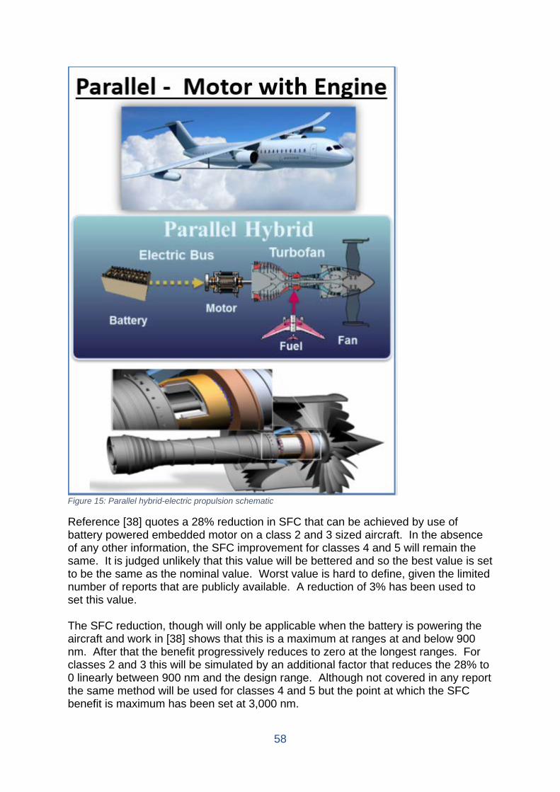
58

Figure 15: Parallel hybrid-electric propulsion schematic

Reference [38] quotes a 28% reduction in SFC that can be achieved by use of battery powered embedded motor on a class 2 and 3 sized aircraft. In the absence of any other information, the SFC improvement for classes 4 and 5 will remain the same. It is judged unlikely that this value will be bettered and so the best value is set to be the same as the nominal value. Worst value is hard to define, given the limited number of reports that are publicly available. A reduction of 3% has been used to set this value. The SFC reduction, though will only be applicable when the battery is powering the aircraft and work in [38] shows that this is a maximum at ranges at and below 900 nm. After that the benefit progressively reduces to zero at the longest ranges. For classes 2 and 3 this will be simulated by an additional factor that reduces the 28% to 0 linearly between 900 nm and the design range. Although not covered in any report the same method will be used for classes 4 and 5 but the point at which the SFC benefit is maximum has been set at 3,000 nm.

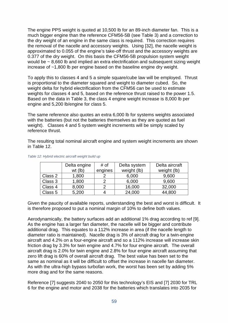
59

The engine PPS weight is quoted at 10,500 lb for an 89-inch diameter fan. This is a much bigger engine than the reference CFM56-5B (see Table 3) and a correction to the dry weight of an engine in the same class is required. This correction requires the removal of the nacelle and accessory weights. Using [32], the nacelle weight is approximated to 0.055 of the engine’s take-off thrust and the accessory weights are 0.377 of the dry weight. On this basis the CFM56-5B propulsion system weight would be ~ 8,660 lb and implied an extra electrification and subsequent sizing weight increase of ~1,800 lb per engine based on the baseline engine dry weight. To apply this to classes 4 and 5 a simple square/cube law will be employed. Thrust is proportional to the diameter squared and weight to diameter cubed. So, the weight delta for hybrid electrification from the CFM56 can be used to estimate weights for classes 4 and 5, based on the reference thrust raised to the power 1.5. Based on the data in Table 3, the class 4 engine weight increase is 8,000 lb per engine and 5,200 lb/engine for class 5. The same reference also quotes an extra 6,000 lb for systems weights associated with the batteries (but not the batteries themselves as they are quoted as fuel weight). Classes 4 and 5 system weight increments will be simply scaled by reference thrust. The resulting total nominal aircraft engine and system weight increments are shown in Table 12. Table 12: Hybrid electric aircraft weight build up

Delta engine wt (lb)

# of engines

Delta system weight (lb)

Delta aircraft weight (lb)

Class 2 1,800 2 6,000 9,600 Class 3 1,800 2 6,000 9,600 Class 4 8,000 2 16,000 32,000 Class 5 5,200 4 24,000 44,800

Given the paucity of available reports, understanding the best and worst is difficult. It is therefore proposed to put a nominal margin of 10% to define both values. Aerodynamically, the battery surfaces add an additional 1% drag according to ref [9]. As the engine has a larger fan diameter, the nacelle will be bigger and contribute additional drag. This equates to a 112% increase in area (if the nacelle length to diameter ratio is maintained). Nacelle drag is 3% of aircraft drag for a twin-engine aircraft and 4.2% on a four-engine aircraft and so a 112% increase will increase skin friction drag by 3.3% for twin engine and 4.7% for four engine aircraft. The overall aircraft drag is 2.0% for twin engine and 2.8% for four engine aircraft assuming that zero lift drag is 60% of overall aircraft drag. The best value has been set to the same as nominal as it will be difficult to offset the increase in nacelle fan diameter. As with the ultra-high bypass turbofan work, the worst has been set by adding 5% more drag and for the same reasons. Reference [7] suggests 2040 to 2050 for this technology’s EIS and [7] 2030 for TRL 6 for the engine and motor and 2038 for the batteries which translates into 2035 for

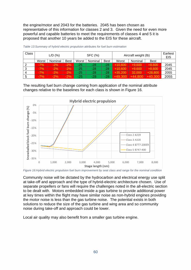
60

the engine/motor and 2043 for the batteries. 2045 has been chosen as representative of this information for classes 2 and 3. Given the need for even more powerful and capable batteries to meet the requirements of classes 4 and 5 it is proposed that another 10 years be added to the EIS for these aircraft. Table 13:Summary of hybrid electric propulsion attributes for fuel burn estimation


Worst Nominal Best Worst Nominal Best Worst Nominal Best 2 -7% -2% -2% -25 -28 -28 +10,600 +9,600 +8,600 2045 3 -7% -2% -2% -25 -28 -28 +10,600 +9,600 +8,600 2045 4 -7% -2% -2% -25 -28 -28 +35,200 32,000 +28,800 2055 5 -7% -2% -2% -25 -28 -28 +49,300 +44,800 +40,300 2055

The resulting fuel burn change coming from application of the nominal attribute changes relative to the baselines for each class is shown in Figure 16.

Figure 16:Hybrid electric propulsion fuel burn improvement by seat class and range for the nominal condition

Community noise will be dictated by the hydrocarbon and electrical energy use split at take-off and approach and the type of hybrid-electric architecture chosen. Use of separate propellers or fans will require the challenges noted in the all-electric section to be dealt with. Motors embedded inside a gas turbine to provide additional power at key times within the flight may have similar noise as non-hybrid engines providing the motor noise is less than the gas turbine noise. The potential exists in both solutions to reduce the size of the gas turbine and wing area and so community noise during take-off and approach could be lower. Local air quality may also benefit from a smaller gas turbine engine.

61

Flying wing On conventional aircraft, the fuselage is a perfect structural way to contain passengers (in pressurised comfort) and cargo. It is, however, aerodynamically very inefficient as it produces a lot of drag but very little lift. The flying wing aims to remove this inefficiency by placing passengers and cargo within the wing and removing as much of the fuselage as possible. This design may also make it possible to remove the horizontal tail. It is anticipated that, as a consequence, a larger improvement in drag will result. There will also be a reduction in weight due to the removal of the fuselage and horizontal tail but the pressurised passenger cabin will no longer be cylindrical and is therefore likely to be much heavier as cylinders are an efficient way to manage forces associated with pressure differences. At this level there are no engine implications and so there will be no change in engine efficiency specially from the flying wing. Reference [5] has developed a large transport flying wing concept (somewhere between class 4 and class 5 categories in capability) that has a 16% improvement in L/D. [40] also looked at a similar aircraft and found an improvement in L/D of between 17.5 and 25%. Reference [41] looked at a very large aircraft and estimated an L/D improvement of 21%. On the smaller side, the flying wing in reference [9] looked at a class 3 sized aircraft and achieved an L/D improvement of 44% but this also included riblets (over the wing body area) and natural laminar flow (over wing and vertical tailplane). It is estimated that around 10% of the overall benefit comes from the riblets and laminar flow and so a value of around 35% could be attributed to the flying wing shape alone. It is also flying much slower at 0.70 cruise Mach number and that will also contribute to the drag improvement seen. For classes 4 and 5 a nominal drag improvement of 17.5% has been taken as a reasonable average of the data found. The best value has been set at 25% being the best value found and the worst has been set at 16% being the worst that has been found. For the smaller aircraft, it is much less clear given the single data point and the additional drag reducing technologies and cruise Mach number. 35% is a long way above the values of the larger aircraft and there is no explanation for why other than the Mach number change. It is proposed to keep the same values used in the larger aircraft in the absence of any other information. Operating empty weight has also been covered by the same references. Reference [5] suggested a weight saving of 34% or 110,000 lb which seems high (and may have been influenced by the aircraft resizing that was undertaken). Reference [40] ended up with a 7,000 lb increase and [41] with a 58,000lb or 12% reduction on one design and 19% on another (but compared against a weight inefficient shrink of the A380). The scatter is very wide and lies around a 10% weight reduction, if the 34% weight reduction is not included. Reference [42] has also looked at this and projects an 11% improvement in aircraft empty weight. On this basis a 31,900 lb reduction

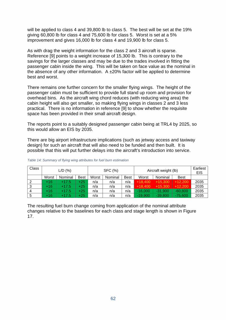
62

will be applied to class 4 and 39,800 lb to class 5. The best will be set at the 19% giving 60,800 lb for class 4 and 75,600 lb for class 5. Worst is set at a 5% improvement and gives 16,000 lb for class 4 and 19,900 lb for class 5. As with drag the weight information for the class 2 and 3 aircraft is sparse. Reference [9] points to a weight increase of 15,300 lb. This is contrary to the savings for the larger classes and may be due to the trades involved in fitting the passenger cabin inside the wing. This will be taken on face value as the nominal in the absence of any other information. A ±20% factor will be applied to determine best and worst. There remains one further concern for the smaller flying wings. The height of the passenger cabin must be sufficient to provide full stand up room and provision for overhead bins. As the aircraft wing chord reduces (with reducing wing area) the cabin height will also get smaller, so making flying wings in classes 2 and 3 less practical. There is no information in reference [9] to show whether the requisite space has been provided in their small aircraft design. The reports point to a suitably designed passenger cabin being at TRL4 by 2025, so this would allow an EIS by 2035. There are big airport infrastructure implications (such as jetway access and taxiway design) for such an aircraft that will also need to be funded and then built. It is possible that this will put further delays into the aircraft’s introduction into service. Table 14: Summary of flying wing attributes for fuel burn estimation


Worst Nominal Best Worst Nominal Best Worst Nominal Best 2 +16 +17.5 +25 n/a n/a n/a +18,400 +15,300 +12,200 2035 3 +16 +17.5 +25 n/a n/a n/a +18,400 +15,300 +12,200 2035 4 +16 +17.5 +25 n/a n/a n/a -16,000 -31,900 -60,800 2035 5 +16 +17.5 +25 n/a n/a n/a -19,900 -39,800 -75,600 2035


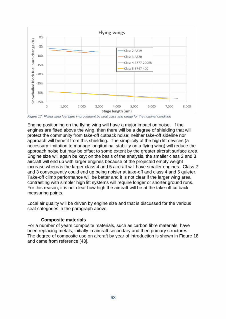
63

Figure 17: Flying wing fuel burn improvement by seat class and range for the nominal condition

Engine positioning on the flying wing will have a major impact on noise. If the engines are fitted above the wing, then there will be a degree of shielding that will protect the community from take-off cutback noise; neither take-off sideline nor approach will benefit from this shielding. The simplicity of the high lift devices (a necessary limitation to manage longitudinal stability on a flying wing) will reduce the approach noise but may be offset to some extent by the greater aircraft surface area. Engine size will again be key; on the basis of the analysis, the smaller class 2 and 3 aircraft will end up with larger engines because of the projected empty weight increase whereas the larger class 4 and 5 aircraft will have smaller engines. Class 2 and 3 consequently could end up being noisier at take-off and class 4 and 5 quieter. Take-off climb performance will be better and it is not clear if the larger wing area contrasting with simpler high lift systems will require longer or shorter ground runs. For this reason, it is not clear how high the aircraft will be at the take-off cutback measuring points. Local air quality will be driven by engine size and that is discussed for the various seat categories in the paragraph above.

Composite materials For a number of years composite materials, such as carbon fibre materials, have been replacing metals, initially in aircraft secondary and then primary structures. The degree of composite use on aircraft by year of introduction is shown in Figure 18 and came from reference [43].

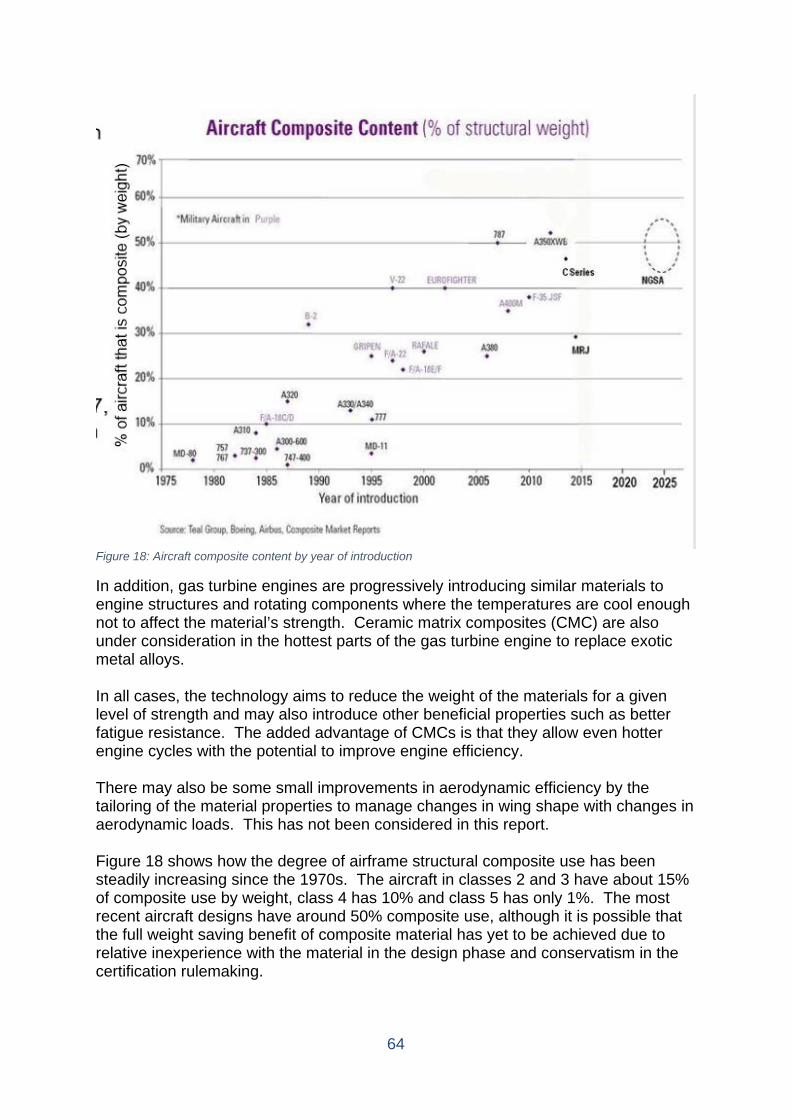
64

Figure 18: Aircraft composite content by year of introduction

In addition, gas turbine engines are progressively introducing similar materials to engine structures and rotating components where the temperatures are cool enough not to affect the material’s strength. Ceramic matrix composites (CMC) are also under consideration in the hottest parts of the gas turbine engine to replace exotic metal alloys. In all cases, the technology aims to reduce the weight of the materials for a given level of strength and may also introduce other beneficial properties such as better fatigue resistance. The added advantage of CMCs is that they allow even hotter engine cycles with the potential to improve engine efficiency. There may also be some small improvements in aerodynamic efficiency by the tailoring of the material properties to manage changes in wing shape with changes in aerodynamic loads. This has not been considered in this report. Figure 18 shows how the degree of airframe structural composite use has been steadily increasing since the 1970s. The aircraft in classes 2 and 3 have about 15% of composite use by weight, class 4 has 10% and class 5 has only 1%. The most recent aircraft designs have around 50% composite use, although it is possible that the full weight saving benefit of composite material has yet to be achieved due to relative inexperience with the material in the design phase and conservatism in the certification rulemaking.

65

Reference [26] suggests that 15% weight saving can be achieved through the use of composites in place of traditional aerospace metals. Reference [9] provides further definition on weight saving potential for different component types and this is shown in Table 15. Table 15: Weight savings for composite by different component types

Strength structure 15%

Stiffness structure 25%

Landing gear 25%

Joining 15% Reference [10] has also explored this technology and suggests that the nominal improvement in 2034 for classes 2, 3, 4 and 5 will be a 17% reduction. Best value for all classes will be 31% and worst value will be 14%. Structural weight reductions of the order of 15 to 25% seem to be common to all references. These are mainly related to engine, airframe and undercarriage structural components. A weight breakdown by major components for each class can be found in reference [32] for transport aircraft and is summarised in Table 16 as a percentage of MTOW (rounded to the nearest percentage point). Table 16: Component group weights relative to maximum take-off weight by seat class

Aircraft type

Wing & controls Fuselage Tail Undercarriage Nacelle Total

Class 2 13% 12% 3% 4% 1% 33%

Class 3 13% 12% 3% 4% 1% 33%

Class 4 16% 11% 2% 4% 2% 35%

Class 5 13% 9% 2% 4% 1% 28% As noted above the aircraft in classes 2 and 3 aircraft have around 15% of current structural weight in composite; class 4 is at 10% and class 5 at 1% and so there are many opportunities in all seat classes. Based on the various reports, it is assumed that 17.5% benefit and 50% of the structure is amenable to use of composites in all classes, then based on the values in Table 16, the resulting weight benefits for the airframe have been estimated and are shown in Table 17.

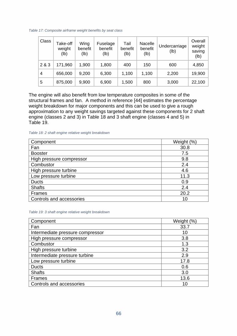
66

Table 17: Composite airframe weight benefits by seat class

Class Take-off weight

(lb)

Wing benefit

(lb)

Fuselage benefit

(lb)

Tail benefit

(lb)

Nacelle benefit

(lb)

Undercarriage (lb)

Overall weight saving

(lb)

2 & 3 171,960 1,900 1,800 400 150 600 4,850

4 656,000 9,200 6,300 1,100 1,100 2,200 19,900

5 875,000 9,900 6,900 1,500 800 3,000 22,100 The engine will also benefit from low temperature composites in some of the structural frames and fan. A method in reference [44] estimates the percentage weight breakdown for major components and this can be used to give a rough approximation to any weight savings targeted against these components for 2 shaft engine (classes 2 and 3) in Table 18 and 3 shaft engine (classes 4 and 5) in Table 19. Table 18: 2 shaft engine relative weight breakdown

Component Weight (%) Fan 30.8 Booster 7.5 High pressure compressor 9.8 Combustor 2.4 High pressure turbine 4.6 Low pressure turbine 11.3 Ducts 0.9 Shafts 2.4 Frames 20.2 Controls and accessories 10

Table 19: 3 shaft engine relative weight breakdown

Component Weight (%) Fan 33.7 Intermediate pressure compressor 10 High pressure compressor 3.8 Combustor 1.3 High pressure turbine 3.2 Intermediate pressure turbine 2.9 Low pressure turbine 17.8 Ducts 0.6 Shafts 3.0 Frames 13.6 Controls and accessories 10

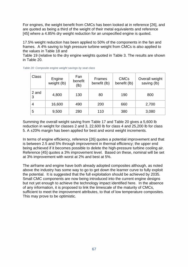
67

For engines, the weight benefit from CMCs has been looked at in reference [26], and are quoted as being a third of the weight of their metal equivalents and reference [45] where a 4.85% dry weight reduction for an unspecified engine is quoted. 17.5% weight reduction has been applied to 50% of the components in the fan and frames. A 4% saving to high pressure turbine weight from CMCs is also applied to the values in Table 18 and Table 19 (relative to the dry engine weights quoted in Table 3. The results are shown in Table 20. Table 20: Composite engine weight savings by seat class

Class Engine weight (lb)

Fan benefit

(lb)

Frames benefit (lb)

CMCs benefit (lb)

Overall weight saving (lb)

2 and 3 4,800 130 80 190 800

4 16,600 490 200 660 2,700

5 9,500 280 110 380 3,080 Summing the overall weight saving from Table 17 and Table 20 gives a 5,600 lb reduction in weight for classes 2 and 3, 22,600 lb for class 4 and 25,200 lb for class 5. A ±20% margin has been applied for best and worst weight increments. In terms of engine efficiency, reference [26] quotes a potential improvement and that is between 2.5 and 5% through improvement in thermal efficiency; the upper end being achieved if it becomes possible to delete the high-pressure turbine cooling air. Reference [45] quotes a 3% improvement level. Based on these, nominal will be set at 3% improvement with worst at 2% and best at 5%. The airframe and engine have both already adopted composites although, as noted above the industry has some way to go to get down the learner curve to fully exploit the potential. It is suggested that the full exploitation should be achieved by 2035. Small CMC components are now being introduced into the current engine designs but not yet enough to achieve the technology impact identified here. In the absence of any information, it is proposed to link the timescale of the maturity of CMCs, sufficient to meet the improvement attributes, to that of low temperature composites. This may prove to be optimistic.

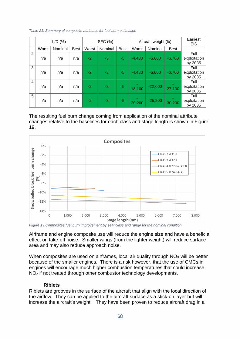
68

Table 21: Summary of composite attributes for fuel burn estimation

L/D (%) SFC (%) Aircraft weight (lb) Earliest

EIS Worst Nominal Best Worst Nominal Best Worst Nominal Best 2

n/a n/a n/a -2 -3 -5 -4,480 -5,600 -6,700 Full

exploitation by 2035

3 n/a n/a n/a -2 -3 -5 -4,480 -5,600 -6,700

Full exploitation

by 2035 4

n/a n/a n/a -2 -3 -5 -18,100 -22,600 -

27,100

Full exploitation

by 2035 5

n/a n/a n/a -2 -3 -5 -20,200 -25,200 -

30,200

Full exploitation

by 2035 The resulting fuel burn change coming from application of the nominal attribute changes relative to the baselines for each class and stage length is shown in Figure 19.

Figure 19:Composites fuel burn improvement by seat class and range for the nominal condition

Airframe and engine composite use will reduce the engine size and have a beneficial effect on take-off noise. Smaller wings (from the lighter weight) will reduce surface area and may also reduce approach noise. When composites are used on airframes, local air quality through NOX will be better because of the smaller engines. There is a risk however, that the use of CMCs in engines will encourage much higher combustion temperatures that could increase NOX if not treated through other combustor technology developments.

Riblets Riblets are grooves in the surface of the aircraft that align with the local direction of the airflow. They can be applied to the aircraft surface as a stick-on layer but will increase the aircraft’s weight. They have been proven to reduce aircraft drag in a

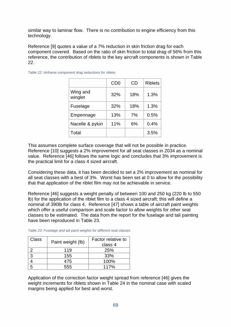
69

similar way to laminar flow. There is no contribution to engine efficiency from this technology. Reference [9] quotes a value of a 7% reduction in skin friction drag for each component covered. Based on the ratio of skin friction to total drag of 56% from this reference, the contribution of riblets to the key aircraft components is shown in Table 22. Table 22: Airframe component drag reductions for riblets

CD0 CD Riblets

Wing and winglet 32% 18% 1.3%

Fuselage 32% 18% 1.3%

Empennage 13% 7% 0.5%

Nacelle & pylon 11% 6% 0.4%

Total 3.5% This assumes complete surface coverage that will not be possible in practice. Reference [10] suggests a 2% improvement for all seat classes in 2034 as a nominal value. Reference [46] follows the same logic and concludes that 3% improvement is the practical limit for a class 4 sized aircraft. Considering these data, it has been decided to set a 2% improvement as nominal for all seat classes with a best of 3%. Worst has been set at 0 to allow for the possibility that that application of the riblet film may not be achievable in service. Reference [46] suggests a weight penalty of between 100 and 250 kg (220 lb to 550 lb) for the application of the riblet film to a class 4 sized aircraft; this will define a nominal of 390lb for class 4. Reference [47] shows a table of aircraft paint weights which offer a useful comparison and scale factor to allow weights for other seat classes to be estimated. The data from the report for the fuselage and tail painting have been reproduced in Table 23. Table 23: Fuselage and tail paint weights for different seat classes

Class Paint weight (lb) Factor relative to class 4

2 119 25% 3 155 33% 4 475 100% 5 555 117%

Application of the correction factor weight spread from reference [46] gives the weight increments for riblets shown in Table 24 in the nominal case with scaled margins being applied for best and worst.

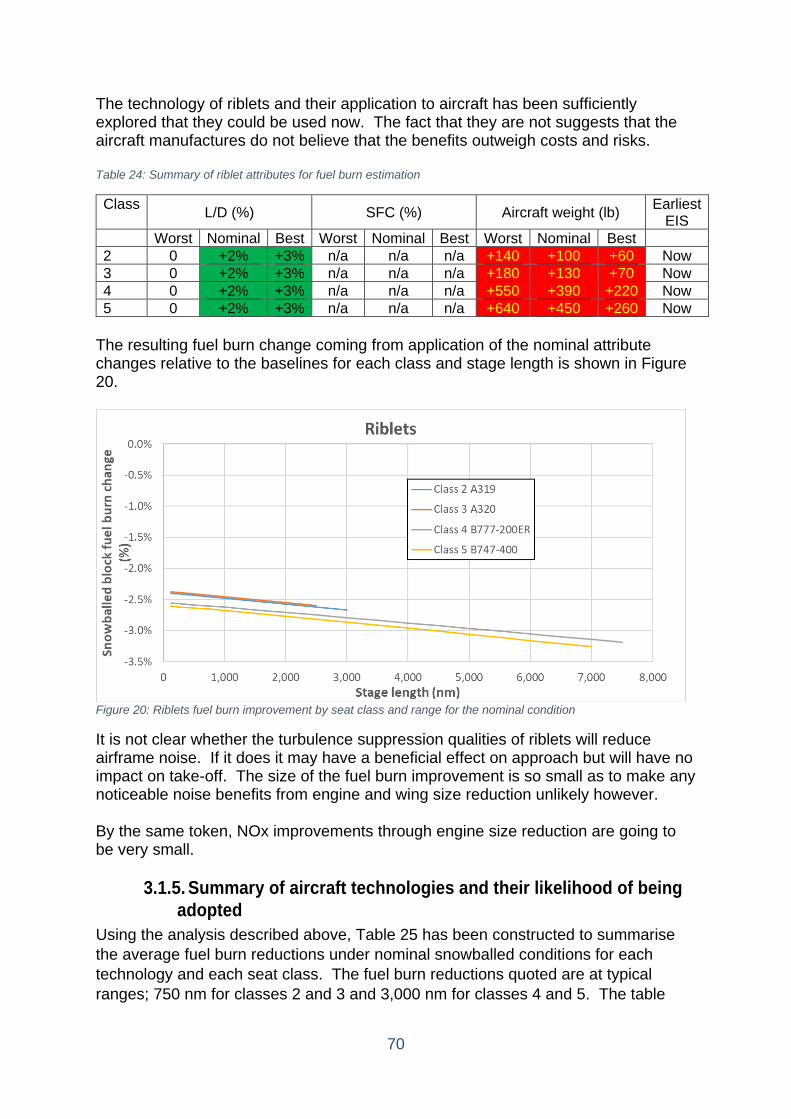
70

The technology of riblets and their application to aircraft has been sufficiently explored that they could be used now. The fact that they are not suggests that the aircraft manufactures do not believe that the benefits outweigh costs and risks. Table 24: Summary of riblet attributes for fuel burn estimation


Worst Nominal Best Worst Nominal Best Worst Nominal Best 2 0 +2% +3% n/a n/a n/a +140 +100 +60 Now 3 0 +2% +3% n/a n/a n/a +180 +130 +70 Now 4 0 +2% +3% n/a n/a n/a +550 +390 +220 Now 5 0 +2% +3% n/a n/a n/a +640 +450 +260 Now


Figure 20: Riblets fuel burn improvement by seat class and range for the nominal condition

It is not clear whether the turbulence suppression qualities of riblets will reduce airframe noise. If it does it may have a beneficial effect on approach but will have no impact on take-off. The size of the fuel burn improvement is so small as to make any noticeable noise benefits from engine and wing size reduction unlikely however. By the same token, NOx improvements through engine size reduction are going to be very small.

3.1.5. Summary of aircraft technologies and their likelihood of being adopted

Using the analysis described above, Table 25 has been constructed to summarise the average fuel burn reductions under nominal snowballed conditions for each technology and each seat class. The fuel burn reductions quoted are at typical ranges; 750 nm for classes 2 and 3 and 3,000 nm for classes 4 and 5. The table

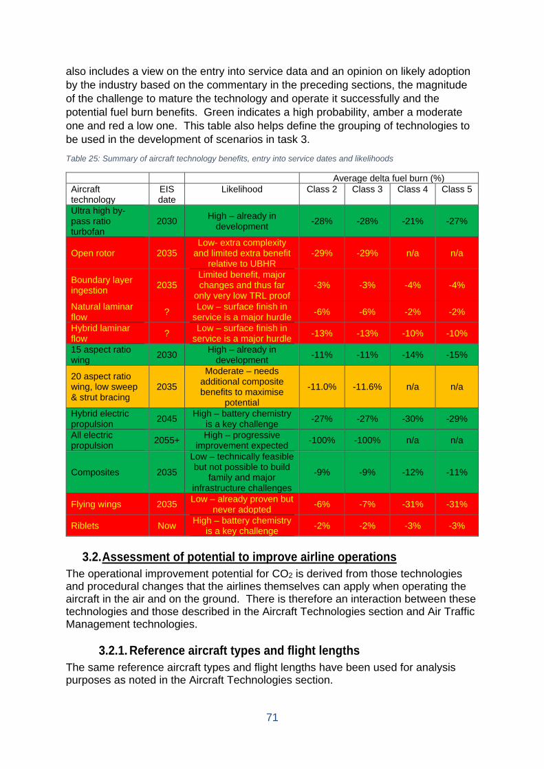
71

also includes a view on the entry into service data and an opinion on likely adoption by the industry based on the commentary in the preceding sections, the magnitude of the challenge to mature the technology and operate it successfully and the potential fuel burn benefits. Green indicates a high probability, amber a moderate one and red a low one. This table also helps define the grouping of technologies to be used in the development of scenarios in task 3. Table 25: Summary of aircraft technology benefits, entry into service dates and likelihoods

Average delta fuel burn (%) Aircraft technology

EIS date

Likelihood Class 2 Class 3 Class 4 Class 5

Ultra high by-pass ratio turbofan

2030 High – already in development -28% -28% -21% -27%

Open rotor 2035 Low- extra complexity

and limited extra benefit relative to UBHR

-29% -29% n/a n/a

Boundary layer ingestion 2035

Limited benefit, major changes and thus far

only very low TRL proof -3% -3% -4% -4%

Natural laminar flow ? Low – surface finish in

service is a major hurdle -6% -6% -2% -2%

Hybrid laminar flow ? Low – surface finish in

service is a major hurdle -13% -13% -10% -10%

15 aspect ratio wing 2030 High – already in

development -11% -11% -14% -15%

20 aspect ratio wing, low sweep & strut bracing

2035

Moderate – needs additional composite benefits to maximise

potential

-11.0% -11.6% n/a n/a

Hybrid electric propulsion 2045 High – battery chemistry

is a key challenge -27% -27% -30% -29%

All electric propulsion 2055+ High – progressive

improvement expected -100% -100% n/a n/a

Composites 2035

Low – technically feasible but not possible to build

family and major infrastructure challenges

-9% -9% -12% -11%

Flying wings 2035 Low – already proven but never adopted -6% -7% -31% -31%

Riblets Now High – battery chemistry is a key challenge -2% -2% -3% -3%

3.2. Assessment of potential to improve airline operations

The operational improvement potential for CO2 is derived from those technologies and procedural changes that the airlines themselves can apply when operating the aircraft in the air and on the ground. There is therefore an interaction between these technologies and those described in the Aircraft Technologies section and Air Traffic Management technologies.

3.2.1. Reference aircraft types and flight lengths The same reference aircraft types and flight lengths have been used for analysis purposes as noted in the Aircraft Technologies section.

72

3.2.2. Improvement to airline operations included in the assessment The technologies and procedures covered in this section are as follows and have been derived from a subject literature search and previous knowledge of areas being researched:

• Formation flying • Long Range Cruise to Maximum Range Cruise speed/Mach number reduction • 0.06 lower cruise Mach number • Engine inoperative taxi • E-tug • E-taxi

3.2.3. Methodology used for the assessment

In the cases of formation flying and 0.06 lower cruise Mach number, the modified Breguet range equation method described in the methodology section has been employed as they both affect the key attributes. The three taxi analysis methods use simple taxi fuel flow data to establish the fuel burn change and the LRC to MRC cruise speed analysis has been assessed by undertaking mission assessments with PIANO-X (reference [48]) in conjunction with a proprietary aircraft performance analysis tool and the modified Breguet method. In all of these cases the fuel burn data are equivalent to a snowballed condition as, with one exception, the aircraft design is not directly affected. In the latter case the data taken from public reports have already been snowballed.

3.2.4. Benefits, timing and uncertainty Formation flying

The idea of formation flying has been taken from migrating bird formations, where a V formation is used as a way of easing the flying workload for the majority of the flock during long flights. In simple terms, correct positioning of one wing tip on the leading aircraft relative to another on the trailing aircraft will reduce the drag of the trailing aircraft, whilst having no impact on the leading aircraft. There is no weight or engine efficiency impact of this approach although aircraft and ATM systems will have to be changed to allow vehicles to fly in very close proximity. The technique will be at its most useful well away from congested airspace and where long periods of straight and level flight are anticipated; cruise conditions on long haul flights are consequently where this is most likely to happen. Reference [49] claims a 12% fuel burn improvement for a 2 aircraft formation based upon a 30% reduction in induced drag and a 40% induced drag contribution to total aircraft drag. This increases to a 40% induced drag change for a 3 aircraft formation. The reference postulates a ±3% error for the first case and ±6% for the second case. Reference [50] also covers this topic and suggests a 5 to 10% fuel burn improvement when applying aerodynamic improvements to real airline flight

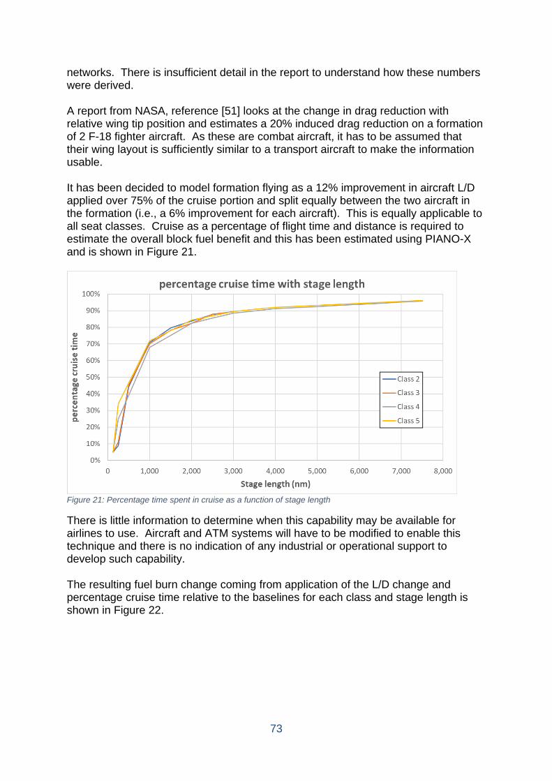
73

networks. There is insufficient detail in the report to understand how these numbers were derived. A report from NASA, reference [51] looks at the change in drag reduction with relative wing tip position and estimates a 20% induced drag reduction on a formation of 2 F-18 fighter aircraft. As these are combat aircraft, it has to be assumed that their wing layout is sufficiently similar to a transport aircraft to make the information usable. It has been decided to model formation flying as a 12% improvement in aircraft L/D applied over 75% of the cruise portion and split equally between the two aircraft in the formation (i.e., a 6% improvement for each aircraft). This is equally applicable to all seat classes. Cruise as a percentage of flight time and distance is required to estimate the overall block fuel benefit and this has been estimated using PIANO-X and is shown in Figure 21.

Figure 21: Percentage time spent in cruise as a function of stage length

There is little information to determine when this capability may be available for airlines to use. Aircraft and ATM systems will have to be modified to enable this technique and there is no indication of any industrial or operational support to develop such capability. The resulting fuel burn change coming from application of the L/D change and percentage cruise time relative to the baselines for each class and stage length is shown in Figure 22.

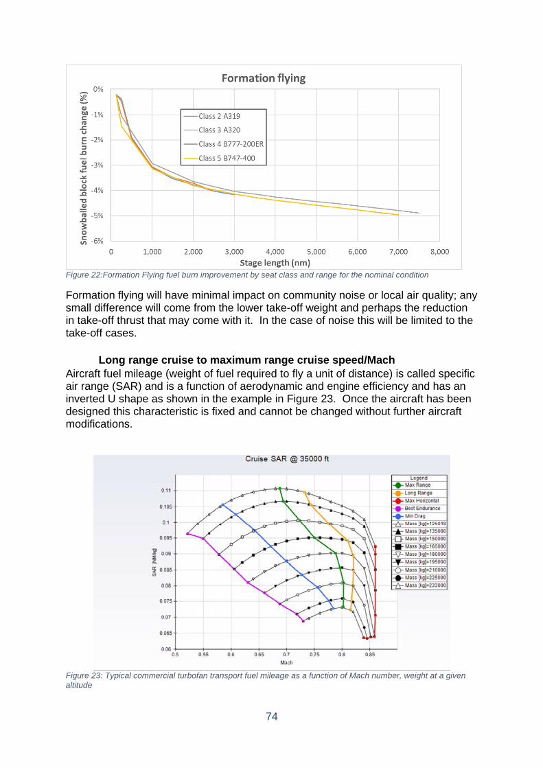
74

Figure 22:Formation Flying fuel burn improvement by seat class and range for the nominal condition

Formation flying will have minimal impact on community noise or local air quality; any small difference will come from the lower take-off weight and perhaps the reduction in take-off thrust that may come with it. In the case of noise this will be limited to the take-off cases.

Long range cruise to maximum range cruise speed/Mach Aircraft fuel mileage (weight of fuel required to fly a unit of distance) is called specific air range (SAR) and is a function of aerodynamic and engine efficiency and has an inverted U shape as shown in the example in Figure 23. Once the aircraft has been designed this characteristic is fixed and cannot be changed without further aircraft modifications.

Figure 23: Typical commercial turbofan transport fuel mileage as a function of Mach number, weight at a given altitude

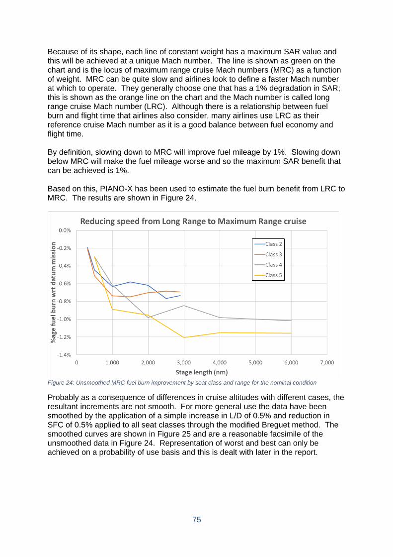
75

Because of its shape, each line of constant weight has a maximum SAR value and this will be achieved at a unique Mach number. The line is shown as green on the chart and is the locus of maximum range cruise Mach numbers (MRC) as a function of weight. MRC can be quite slow and airlines look to define a faster Mach number at which to operate. They generally choose one that has a 1% degradation in SAR; this is shown as the orange line on the chart and the Mach number is called long range cruise Mach number (LRC). Although there is a relationship between fuel burn and flight time that airlines also consider, many airlines use LRC as their reference cruise Mach number as it is a good balance between fuel economy and flight time. By definition, slowing down to MRC will improve fuel mileage by 1%. Slowing down below MRC will make the fuel mileage worse and so the maximum SAR benefit that can be achieved is 1%. Based on this, PIANO-X has been used to estimate the fuel burn benefit from LRC to MRC. The results are shown in Figure 24.

Figure 24: Unsmoothed MRC fuel burn improvement by seat class and range for the nominal condition

Probably as a consequence of differences in cruise altitudes with different cases, the resultant increments are not smooth. For more general use the data have been smoothed by the application of a simple increase in L/D of 0.5% and reduction in SFC of 0.5% applied to all seat classes through the modified Breguet method. The smoothed curves are shown in Figure 25 and are a reasonable facsimile of the unsmoothed data in Figure 24. Representation of worst and best can only be achieved on a probability of use basis and this is dealt with later in the report.

76

Figure 25: Smoothed MRC fuel burn improvement by seat class and range for the nominal condition

Airlines can use this technique today as there are no aircraft changes required and the ATM system is well able to cope with the speed variations it creates. The implementation in the cockpit is via a dedicated function within the Flight Management System (FMS). Moving from LRC to MRC will have minimal impact on community noise or local air quality; any difference will come from the lower take-off weight and perhaps the reduction in take-off thrust that may come with it. In the case of noise this will be limited to the take-off cases.

Aircraft design for 0.06 lower cruise Mach number Given the very limited benefit for reducing cruise Mach number on existing aircraft, the other option is to design new aircraft to operate at lower Mach numbers from the outset. This will reduce the aircraft drag and hence the thrust required; the engine will be smaller and lighter and the wing sweep can be reduced further reducing weight and improving aerodynamics. The engine is also more fuel efficient at lower speeds. All of these factors work together to significantly reduce the aircraft size and weight and reduce fuel burn for the same mission. Aircraft in seat classes 2 and 3 currently operate at around 0.78Mach in cruise; class 4 at 0.84Mach and class 5 at 0.85Mach. A nominal reduction of 0.06 reduction in cruise Mach number has been assessed based on a number of public reports for all of these classes and cruise Mach numbers. This equates to an 8% reduction for classes 2 and 3 and a 7% reduction for classes 4 and 5. The Mach number reduction will increase block time (see Figure 4) and may reduce the number of flights per day (see Figure 5), there may also be mitigations from some of the Operational improvements (covered in section 3.3) such as optimum track that could offset the operational penalties of reduced Cruise Mach number. References [5] and [6] show the impact of moving from cruise at 0.78Mach number to 0.72Mach number on a 737-800 aircraft design (similar to classes 2 and 3) in

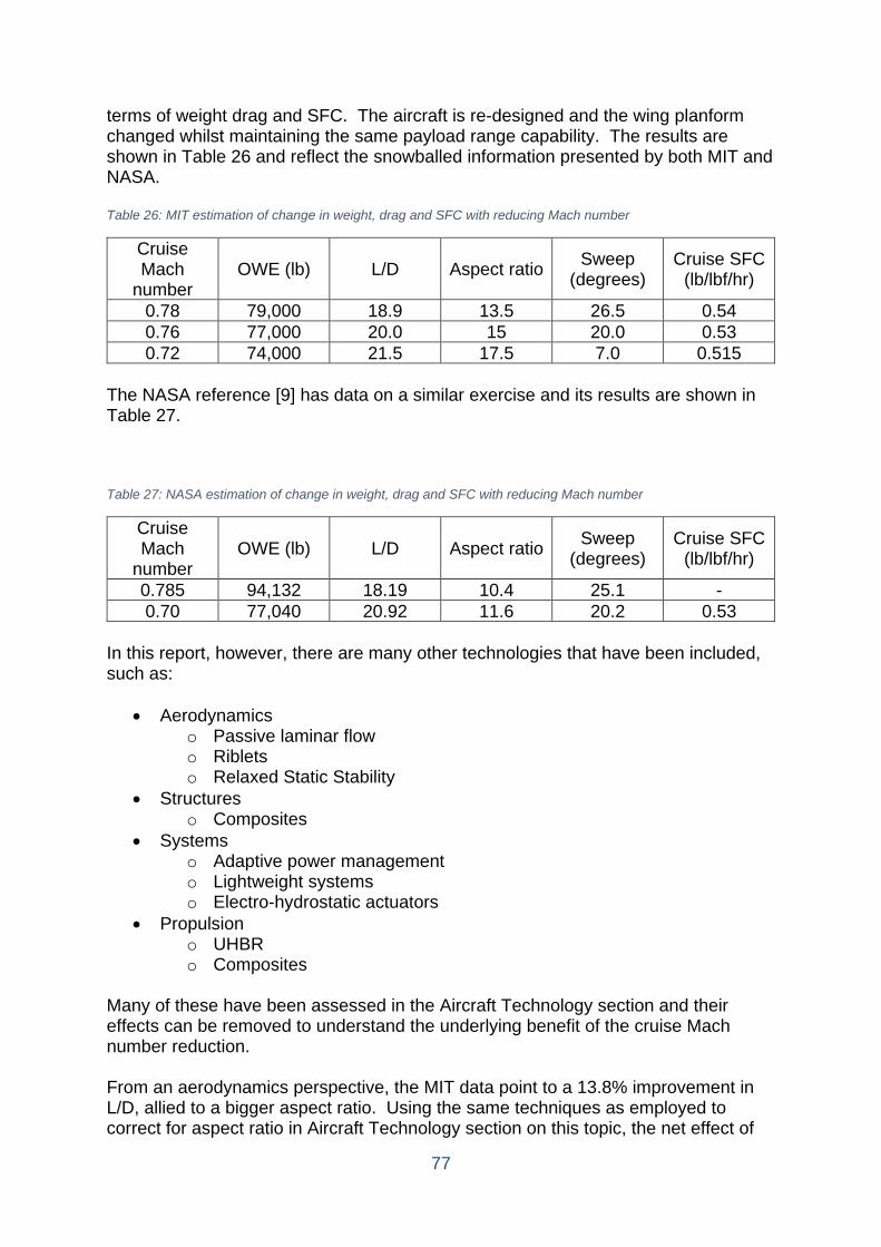
77

terms of weight drag and SFC. The aircraft is re-designed and the wing planform changed whilst maintaining the same payload range capability. The results are shown in Table 26 and reflect the snowballed information presented by both MIT and NASA. Table 26: MIT estimation of change in weight, drag and SFC with reducing Mach number

Cruise Mach

number OWE (lb) L/D Aspect ratio Sweep

(degrees) Cruise SFC

(lb/lbf/hr)

0.78 79,000 18.9 13.5 26.5 0.54 0.76 77,000 20.0 15 20.0 0.53 0.72 74,000 21.5 17.5 7.0 0.515

The NASA reference [9] has data on a similar exercise and its results are shown in Table 27. Table 27: NASA estimation of change in weight, drag and SFC with reducing Mach number

Cruise Mach

number OWE (lb) L/D Aspect ratio Sweep

(degrees) Cruise SFC

(lb/lbf/hr)

0.785 94,132 18.19 10.4 25.1 - 0.70 77,040 20.92 11.6 20.2 0.53

In this report, however, there are many other technologies that have been included, such as:

• Aerodynamics o Passive laminar flow o Riblets o Relaxed Static Stability

• Structures o Composites

• Systems o Adaptive power management o Lightweight systems o Electro-hydrostatic actuators

• Propulsion o UHBR o Composites

Many of these have been assessed in the Aircraft Technology section and their effects can be removed to understand the underlying benefit of the cruise Mach number reduction. From an aerodynamics perspective, the MIT data point to a 13.8% improvement in L/D, allied to a bigger aspect ratio. Using the same techniques as employed to correct for aspect ratio in Aircraft Technology section on this topic, the net effect of

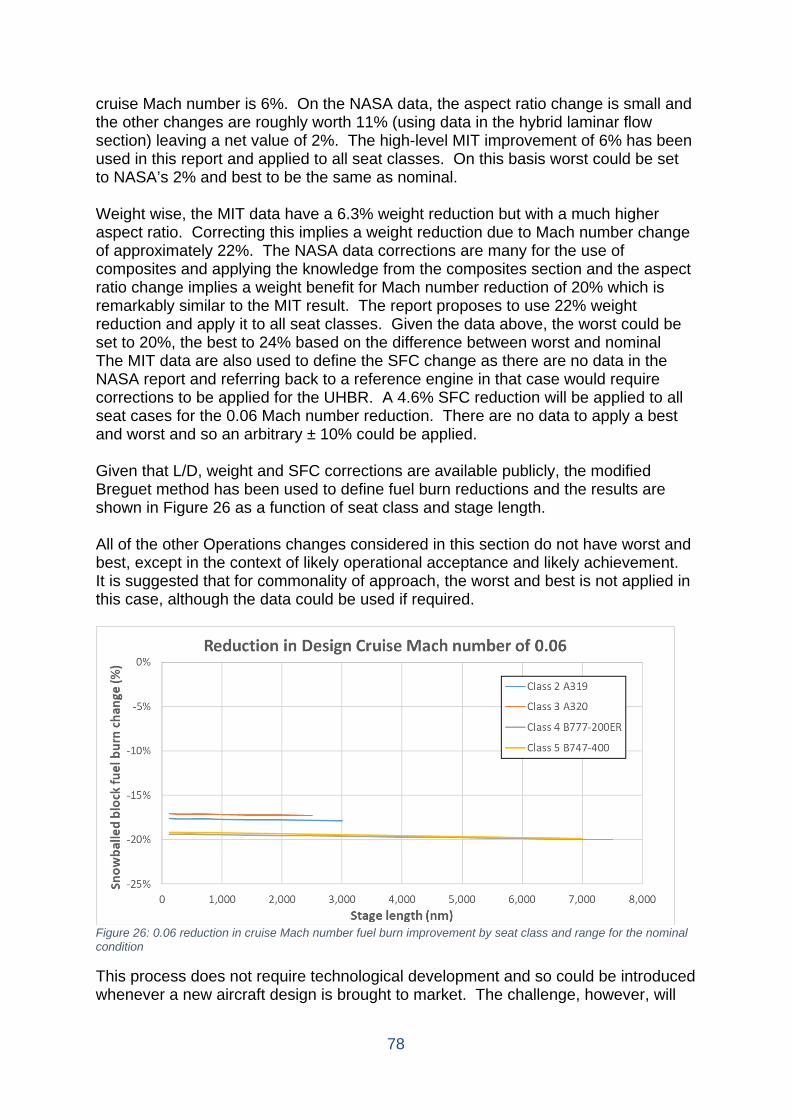
78

cruise Mach number is 6%. On the NASA data, the aspect ratio change is small and the other changes are roughly worth 11% (using data in the hybrid laminar flow section) leaving a net value of 2%. The high-level MIT improvement of 6% has been used in this report and applied to all seat classes. On this basis worst could be set to NASA’s 2% and best to be the same as nominal. Weight wise, the MIT data have a 6.3% weight reduction but with a much higher aspect ratio. Correcting this implies a weight reduction due to Mach number change of approximately 22%. The NASA data corrections are many for the use of composites and applying the knowledge from the composites section and the aspect ratio change implies a weight benefit for Mach number reduction of 20% which is remarkably similar to the MIT result. The report proposes to use 22% weight reduction and apply it to all seat classes. Given the data above, the worst could be set to 20%, the best to 24% based on the difference between worst and nominal The MIT data are also used to define the SFC change as there are no data in the NASA report and referring back to a reference engine in that case would require corrections to be applied for the UHBR. A 4.6% SFC reduction will be applied to all seat cases for the 0.06 Mach number reduction. There are no data to apply a best and worst and so an arbitrary ± 10% could be applied. Given that L/D, weight and SFC corrections are available publicly, the modified Breguet method has been used to define fuel burn reductions and the results are shown in Figure 26 as a function of seat class and stage length. All of the other Operations changes considered in this section do not have worst and best, except in the context of likely operational acceptance and likely achievement. It is suggested that for commonality of approach, the worst and best is not applied in this case, although the data could be used if required.

Figure 26: 0.06 reduction in cruise Mach number fuel burn improvement by seat class and range for the nominal condition

This process does not require technological development and so could be introduced whenever a new aircraft design is brought to market. The challenge, however, will

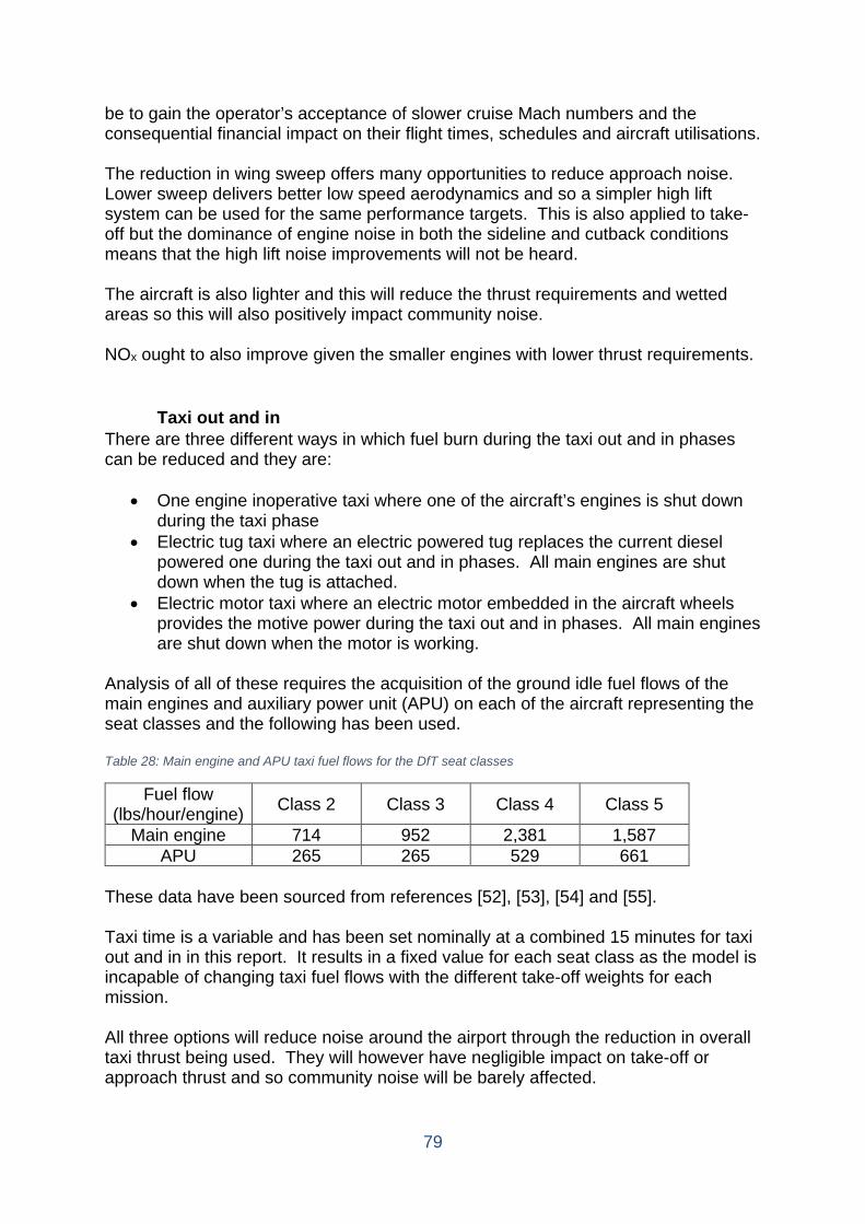
79

be to gain the operator’s acceptance of slower cruise Mach numbers and the consequential financial impact on their flight times, schedules and aircraft utilisations. The reduction in wing sweep offers many opportunities to reduce approach noise. Lower sweep delivers better low speed aerodynamics and so a simpler high lift system can be used for the same performance targets. This is also applied to take-off but the dominance of engine noise in both the sideline and cutback conditions means that the high lift noise improvements will not be heard. The aircraft is also lighter and this will reduce the thrust requirements and wetted areas so this will also positively impact community noise. NOx ought to also improve given the smaller engines with lower thrust requirements.

Taxi out and in There are three different ways in which fuel burn during the taxi out and in phases can be reduced and they are:

• One engine inoperative taxi where one of the aircraft’s engines is shut down during the taxi phase

• Electric tug taxi where an electric powered tug replaces the current diesel powered one during the taxi out and in phases. All main engines are shut down when the tug is attached.

• Electric motor taxi where an electric motor embedded in the aircraft wheels provides the motive power during the taxi out and in phases. All main engines are shut down when the motor is working.

Analysis of all of these requires the acquisition of the ground idle fuel flows of the main engines and auxiliary power unit (APU) on each of the aircraft representing the seat classes and the following has been used. Table 28: Main engine and APU taxi fuel flows for the DfT seat classes

Fuel flow (lbs/hour/engine) Class 2 Class 3 Class 4 Class 5

Main engine 714 952 2,381 1,587 APU 265 265 529 661

These data have been sourced from references [52], [53], [54] and [55]. Taxi time is a variable and has been set nominally at a combined 15 minutes for taxi out and in in this report. It results in a fixed value for each seat class as the model is incapable of changing taxi fuel flows with the different take-off weights for each mission. All three options will reduce noise around the airport through the reduction in overall taxi thrust being used. They will however have negligible impact on take-off or approach thrust and so community noise will be barely affected.

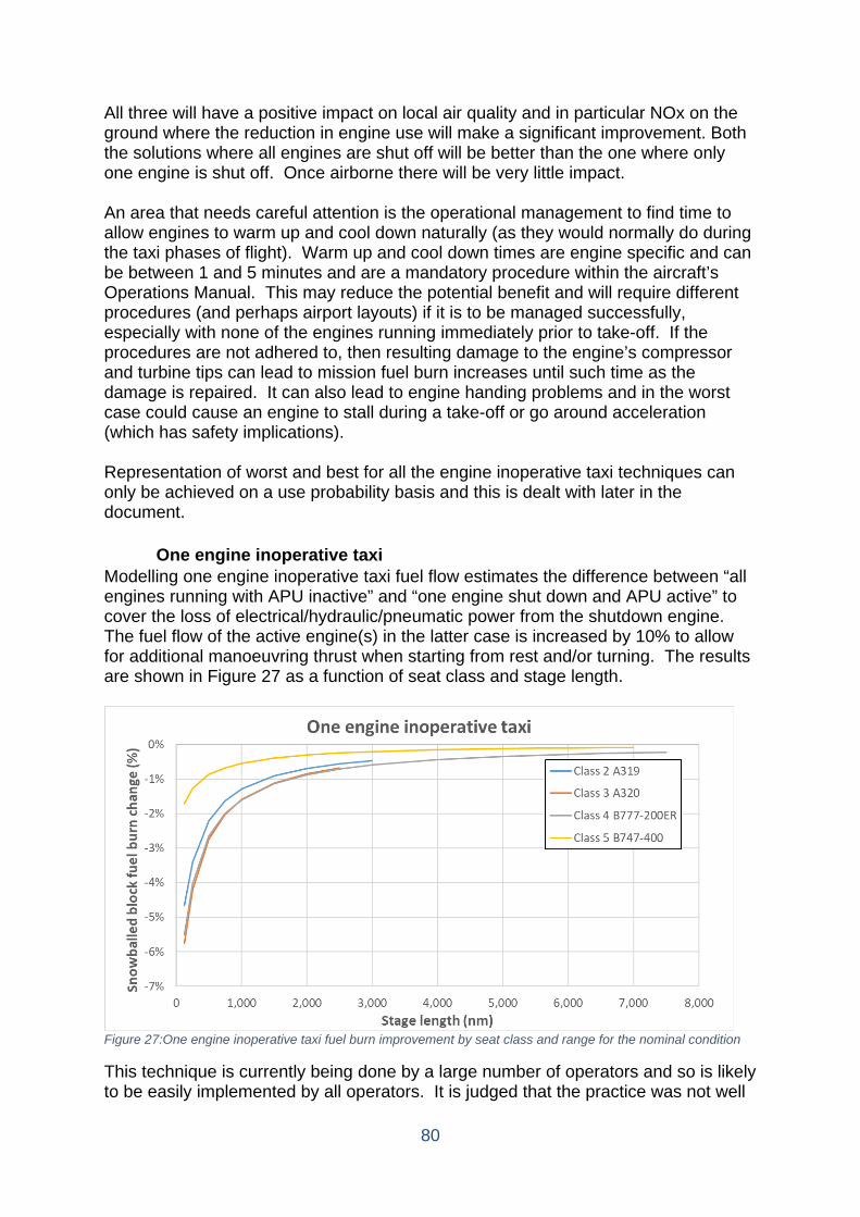
80

All three will have a positive impact on local air quality and in particular NOx on the ground where the reduction in engine use will make a significant improvement. Both the solutions where all engines are shut off will be better than the one where only one engine is shut off. Once airborne there will be very little impact. An area that needs careful attention is the operational management to find time to allow engines to warm up and cool down naturally (as they would normally do during the taxi phases of flight). Warm up and cool down times are engine specific and can be between 1 and 5 minutes and are a mandatory procedure within the aircraft’s Operations Manual. This may reduce the potential benefit and will require different procedures (and perhaps airport layouts) if it is to be managed successfully, especially with none of the engines running immediately prior to take-off. If the procedures are not adhered to, then resulting damage to the engine’s compressor and turbine tips can lead to mission fuel burn increases until such time as the damage is repaired. It can also lead to engine handing problems and in the worst case could cause an engine to stall during a take-off or go around acceleration (which has safety implications). Representation of worst and best for all the engine inoperative taxi techniques can only be achieved on a use probability basis and this is dealt with later in the document.

One engine inoperative taxi Modelling one engine inoperative taxi fuel flow estimates the difference between “all engines running with APU inactive” and “one engine shut down and APU active” to cover the loss of electrical/hydraulic/pneumatic power from the shutdown engine. The fuel flow of the active engine(s) in the latter case is increased by 10% to allow for additional manoeuvring thrust when starting from rest and/or turning. The results are shown in Figure 27 as a function of seat class and stage length.

Figure 27:One engine inoperative taxi fuel burn improvement by seat class and range for the nominal condition

This technique is currently being done by a large number of operators and so is likely to be easily implemented by all operators. It is judged that the practice was not well

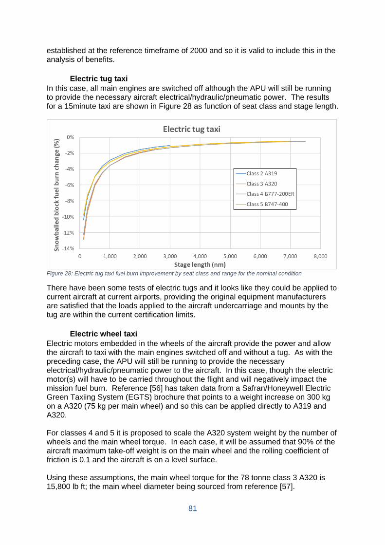
81

established at the reference timeframe of 2000 and so it is valid to include this in the analysis of benefits.

Electric tug taxi In this case, all main engines are switched off although the APU will still be running to provide the necessary aircraft electrical/hydraulic/pneumatic power. The results for a 15minute taxi are shown in Figure 28 as function of seat class and stage length.

Figure 28: Electric tug taxi fuel burn improvement by seat class and range for the nominal condition

There have been some tests of electric tugs and it looks like they could be applied to current aircraft at current airports, providing the original equipment manufacturers are satisfied that the loads applied to the aircraft undercarriage and mounts by the tug are within the current certification limits.

Electric wheel taxi Electric motors embedded in the wheels of the aircraft provide the power and allow the aircraft to taxi with the main engines switched off and without a tug. As with the preceding case, the APU will still be running to provide the necessary electrical/hydraulic/pneumatic power to the aircraft. In this case, though the electric motor(s) will have to be carried throughout the flight and will negatively impact the mission fuel burn. Reference [56] has taken data from a Safran/Honeywell Electric Green Taxiing System (EGTS) brochure that points to a weight increase on 300 kg on a A320 (75 kg per main wheel) and so this can be applied directly to A319 and A320. For classes 4 and 5 it is proposed to scale the A320 system weight by the number of wheels and the main wheel torque. In each case, it will be assumed that 90% of the aircraft maximum take-off weight is on the main wheel and the rolling coefficient of friction is 0.1 and the aircraft is on a level surface. Using these assumptions, the main wheel torque for the 78 tonne class 3 A320 is 15,800 lb ft; the main wheel diameter being sourced from reference [57].

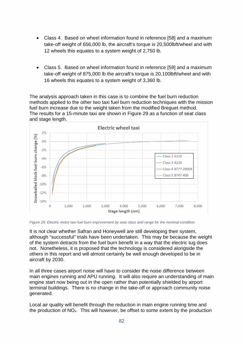
82

• Class 4. Based on wheel information found in reference [58] and a maximum

take-off weight of 656,000 lb, the aircraft’s torque is 20,500lbft/wheel and with 12 wheels this equates to a system weight of 2,750 lb.

• Class 5. Based on wheel information found in reference [59] and a maximum

take-off weight of 875,000 lb the aircraft’s torque is 20,100lbft/wheel and with 16 wheels this equates to a system weight of 3,360 lb.

The analysis approach taken in this case is to combine the fuel burn reduction methods applied to the other two taxi fuel burn reduction techniques with the mission fuel burn increase due to the weight taken from the modified Breguet method. The results for a 15-minute taxi are shown in Figure 29 as a function of seat class and stage length.

Figure 29: Electric motor taxi fuel burn improvement by seat class and range for the nominal condition

It is not clear whether Safran and Honeywell are still developing their system, although “successful” trials have been undertaken. This may be because the weight of the system detracts from the fuel burn benefit in a way that the electric tug does not. Nonetheless, it is proposed that the technology is considered alongside the others in this report and will almost certainly be well enough developed to be in aircraft by 2030. In all three cases airport noise will have to consider the noise difference between main engines running and APU running. It will also require an understanding of main engine start now being out in the open rather than potentially shielded by airport terminal buildings. There is no change in the take-off or approach community noise generated. Local air quality will benefit through the reduction in main engine running time and the production of NOx. This will however, be offset to some extent by the production

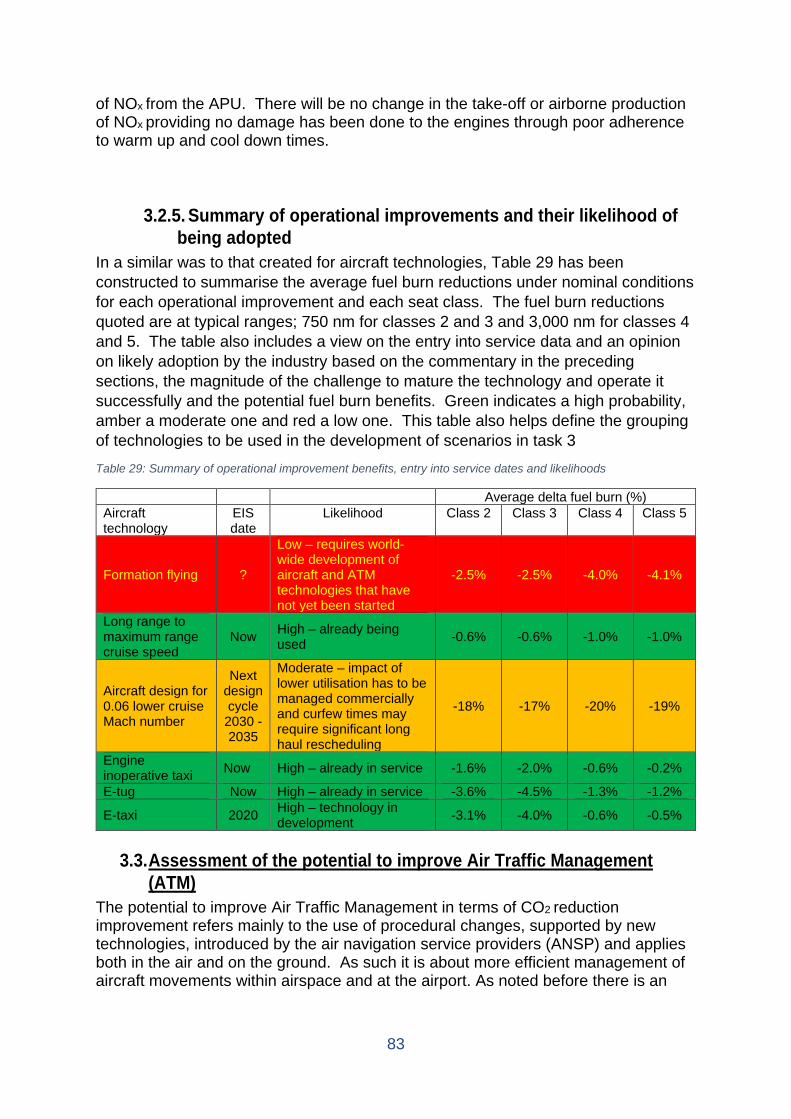
83

of NOx from the APU. There will be no change in the take-off or airborne production of NOx providing no damage has been done to the engines through poor adherence to warm up and cool down times.

3.2.5. Summary of operational improvements and their likelihood of being adopted

In a similar was to that created for aircraft technologies, Table 29 has been constructed to summarise the average fuel burn reductions under nominal conditions for each operational improvement and each seat class. The fuel burn reductions quoted are at typical ranges; 750 nm for classes 2 and 3 and 3,000 nm for classes 4 and 5. The table also includes a view on the entry into service data and an opinion on likely adoption by the industry based on the commentary in the preceding sections, the magnitude of the challenge to mature the technology and operate it successfully and the potential fuel burn benefits. Green indicates a high probability, amber a moderate one and red a low one. This table also helps define the grouping of technologies to be used in the development of scenarios in task 3 Table 29: Summary of operational improvement benefits, entry into service dates and likelihoods


EIS date

Likelihood Class 2 Class 3 Class 4 Class 5

Formation flying ?

Low – requires world-wide development of aircraft and ATM technologies that have not yet been started

-2.5% -2.5% -4.0% -4.1%

Long range to maximum range cruise speed

Now High – already being used -0.6% -0.6% -1.0% -1.0%

Aircraft design for 0.06 lower cruise Mach number

Next design cycle 2030 -2035

Moderate – impact of lower utilisation has to be managed commercially and curfew times may require significant long haul rescheduling

-18% -17% -20% -19%

Engine inoperative taxi Now High – already in service -1.6% -2.0% -0.6% -0.2%

E-tug Now High – already in service -3.6% -4.5% -1.3% -1.2%

E-taxi 2020 High – technology in development -3.1% -4.0% -0.6% -0.5%

3.3. Assessment of the potential to improve Air Traffic Management

(ATM) The potential to improve Air Traffic Management in terms of CO2 reduction improvement refers mainly to the use of procedural changes, supported by new technologies, introduced by the air navigation service providers (ANSP) and applies both in the air and on the ground. As such it is about more efficient management of aircraft movements within airspace and at the airport. As noted before there is an

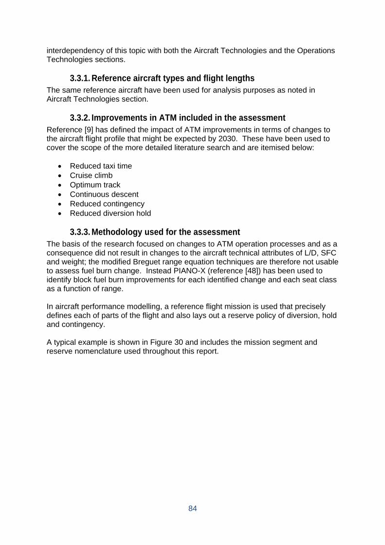
84

interdependency of this topic with both the Aircraft Technologies and the Operations Technologies sections.

3.3.1. Reference aircraft types and flight lengths The same reference aircraft have been used for analysis purposes as noted in Aircraft Technologies section.

3.3.2. Improvements in ATM included in the assessment Reference [9] has defined the impact of ATM improvements in terms of changes to the aircraft flight profile that might be expected by 2030. These have been used to cover the scope of the more detailed literature search and are itemised below:

• Reduced taxi time • Cruise climb • Optimum track • Continuous descent • Reduced contingency • Reduced diversion hold

3.3.3. Methodology used for the assessment

The basis of the research focused on changes to ATM operation processes and as a consequence did not result in changes to the aircraft technical attributes of L/D, SFC and weight; the modified Breguet range equation techniques are therefore not usable to assess fuel burn change. Instead PIANO-X (reference [48]) has been used to identify block fuel burn improvements for each identified change and each seat class as a function of range. In aircraft performance modelling, a reference flight mission is used that precisely defines each of parts of the flight and also lays out a reserve policy of diversion, hold and contingency. A typical example is shown in Figure 30 and includes the mission segment and reserve nomenclature used throughout this report.

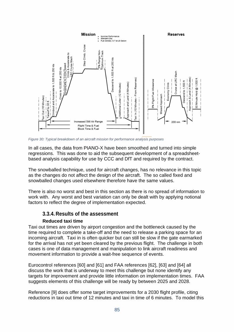
85

Figure 30: Typical breakdown of an aircraft mission for performance analysis purposes

In all cases, the data from PIANO-X have been smoothed and turned into simple regressions. This was done to aid the subsequent development of a spreadsheet-based analysis capability for use by CCC and DfT and required by the contract. The snowballed technique, used for aircraft changes, has no relevance in this topic as the changes do not affect the design of the aircraft. The so called fixed and snowballed changes used elsewhere therefore have the same values. There is also no worst and best in this section as there is no spread of information to work with. Any worst and best variation can only be dealt with by applying notional factors to reflect the degree of implementation expected.

3.3.4. Results of the assessment Reduced taxi time

Taxi out times are driven by airport congestion and the bottleneck caused by the time required to complete a take-off and the need to release a parking space for an incoming aircraft. Taxi in is often quicker but can still be slow if the gate earmarked for the arrival has not yet been cleared by the previous flight. The challenge in both cases is one of data management and manipulation to link aircraft readiness and movement information to provide a wait-free sequence of events. Eurocontrol references [60] and [61] and FAA references [62], [63] and [64] all discuss the work that is underway to meet this challenge but none identify any targets for improvement and provide little information on implementation times. FAA suggests elements of this challenge will be ready by between 2025 and 2028. Reference [9] does offer some target improvements for a 2030 flight profile, citing reductions in taxi out time of 12 minutes and taxi in time of 6 minutes. To model this

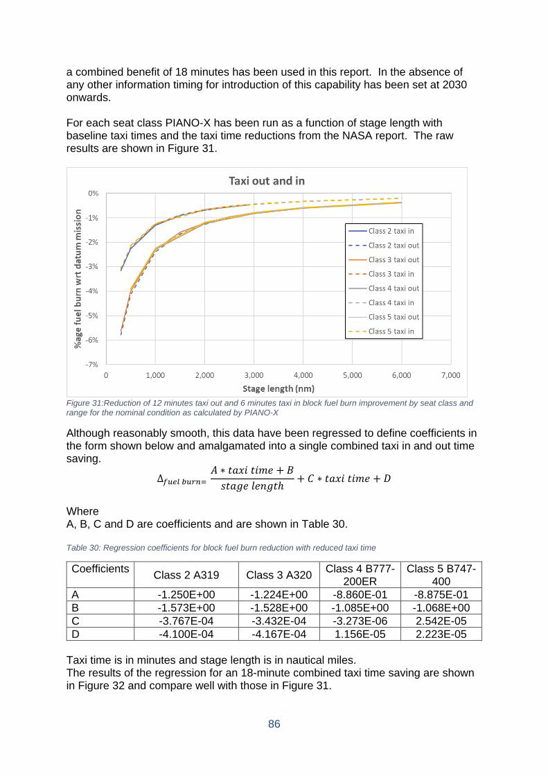
86

a combined benefit of 18 minutes has been used in this report. In the absence of any other information timing for introduction of this capability has been set at 2030 onwards. For each seat class PIANO-X has been run as a function of stage length with baseline taxi times and the taxi time reductions from the NASA report. The raw results are shown in Figure 31.

Figure 31:Reduction of 12 minutes taxi out and 6 minutes taxi in block fuel burn improvement by seat class and range for the nominal condition as calculated by PIANO-X

Although reasonably smooth, this data have been regressed to define coefficients in the form shown below and amalgamated into a single combined taxi in and out time saving.

∆𝑓𝑓𝑓𝑓𝑓𝑓𝑓𝑓 𝑏𝑏𝑓𝑓𝑏𝑏𝑏𝑏= 𝐴𝐴 ∗ 𝑓𝑓𝑟𝑟𝑡𝑡𝑡𝑡 𝑓𝑓𝑡𝑡𝑡𝑡𝑟𝑟 + 𝐵𝐵𝑠𝑠𝑓𝑓𝑟𝑟𝑟𝑟𝑟𝑟 𝑙𝑙𝑟𝑟𝑙𝑙𝑟𝑟𝑓𝑓ℎ

+ 𝑆𝑆 ∗ 𝑓𝑓𝑟𝑟𝑡𝑡𝑡𝑡 𝑓𝑓𝑡𝑡𝑡𝑡𝑟𝑟 + 𝐷𝐷

Where A, B, C and D are coefficients and are shown in Table 30. Table 30: Regression coefficients for block fuel burn reduction with reduced taxi time

Coefficients Class 2 A319 Class 3 A320 Class 4 B777-200ER

Class 5 B747-400

A -1.250E+00 -1.224E+00 -8.860E-01 -8.875E-01 B -1.573E+00 -1.528E+00 -1.085E+00 -1.068E+00 C -3.767E-04 -3.432E-04 -3.273E-06 2.542E-05 D -4.100E-04 -4.167E-04 1.156E-05 2.223E-05

Taxi time is in minutes and stage length is in nautical miles. The results of the regression for an 18-minute combined taxi time saving are shown in Figure 32 and compare well with those in Figure 31.

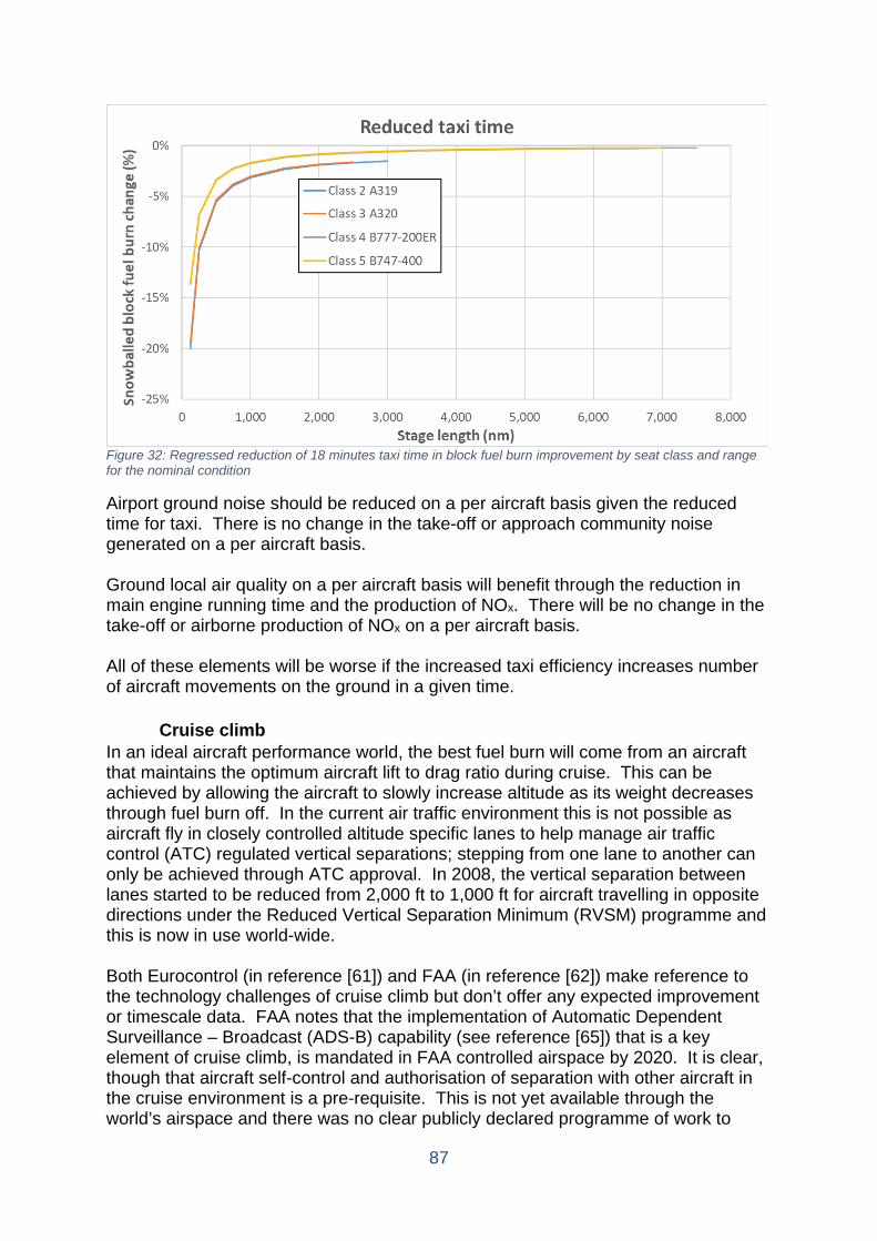
87

Figure 32: Regressed reduction of 18 minutes taxi time in block fuel burn improvement by seat class and range for the nominal condition

Airport ground noise should be reduced on a per aircraft basis given the reduced time for taxi. There is no change in the take-off or approach community noise generated on a per aircraft basis. Ground local air quality on a per aircraft basis will benefit through the reduction in main engine running time and the production of NOx. There will be no change in the take-off or airborne production of NOx on a per aircraft basis. All of these elements will be worse if the increased taxi efficiency increases number of aircraft movements on the ground in a given time.

Cruise climb In an ideal aircraft performance world, the best fuel burn will come from an aircraft that maintains the optimum aircraft lift to drag ratio during cruise. This can be achieved by allowing the aircraft to slowly increase altitude as its weight decreases through fuel burn off. In the current air traffic environment this is not possible as aircraft fly in closely controlled altitude specific lanes to help manage air traffic control (ATC) regulated vertical separations; stepping from one lane to another can only be achieved through ATC approval. In 2008, the vertical separation between lanes started to be reduced from 2,000 ft to 1,000 ft for aircraft travelling in opposite directions under the Reduced Vertical Separation Minimum (RVSM) programme and this is now in use world-wide. Both Eurocontrol (in reference [61]) and FAA (in reference [62]) make reference to the technology challenges of cruise climb but don’t offer any expected improvement or timescale data. FAA notes that the implementation of Automatic Dependent Surveillance – Broadcast (ADS-B) capability (see reference [65]) that is a key element of cruise climb, is mandated in FAA controlled airspace by 2020. It is clear, though that aircraft self-control and authorisation of separation with other aircraft in the cruise environment is a pre-requisite. This is not yet available through the world’s airspace and there was no clear publicly declared programme of work to

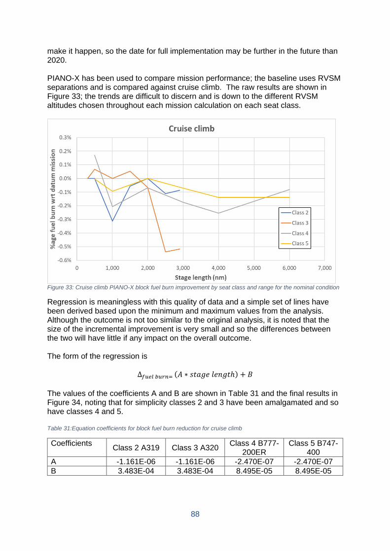
88

make it happen, so the date for full implementation may be further in the future than 2020. PIANO-X has been used to compare mission performance; the baseline uses RVSM separations and is compared against cruise climb. The raw results are shown in Figure 33; the trends are difficult to discern and is down to the different RVSM altitudes chosen throughout each mission calculation on each seat class.

Figure 33: Cruise climb PIANO-X block fuel burn improvement by seat class and range for the nominal condition

Regression is meaningless with this quality of data and a simple set of lines have been derived based upon the minimum and maximum values from the analysis. Although the outcome is not too similar to the original analysis, it is noted that the size of the incremental improvement is very small and so the differences between the two will have little if any impact on the overall outcome. The form of the regression is

∆𝑓𝑓𝑓𝑓𝑓𝑓𝑓𝑓 𝑏𝑏𝑓𝑓𝑏𝑏𝑏𝑏= (𝐴𝐴 ∗ 𝑠𝑠𝑓𝑓𝑟𝑟𝑟𝑟𝑟𝑟 𝑙𝑙𝑟𝑟𝑙𝑙𝑟𝑟𝑓𝑓ℎ) + 𝐵𝐵 The values of the coefficients A and B are shown in Table 31 and the final results in Figure 34, noting that for simplicity classes 2 and 3 have been amalgamated and so have classes 4 and 5. Table 31:Equation coefficients for block fuel burn reduction for cruise climb


Class 5 B747-400

A -1.161E-06 -1.161E-06 -2.470E-07 -2.470E-07 B 3.483E-04 3.483E-04 8.495E-05 8.495E-05

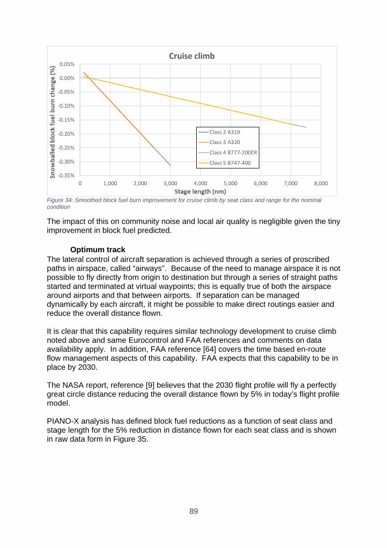
89

Figure 34: Smoothed block fuel burn improvement for cruise climb by seat class and range for the nominal condition

The impact of this on community noise and local air quality is negligible given the tiny improvement in block fuel predicted.

Optimum track The lateral control of aircraft separation is achieved through a series of proscribed paths in airspace, called “airways”. Because of the need to manage airspace it is not possible to fly directly from origin to destination but through a series of straight paths started and terminated at virtual waypoints; this is equally true of both the airspace around airports and that between airports. If separation can be managed dynamically by each aircraft, it might be possible to make direct routings easier and reduce the overall distance flown. It is clear that this capability requires similar technology development to cruise climb noted above and same Eurocontrol and FAA references and comments on data availability apply. In addition, FAA reference [64] covers the time based en-route flow management aspects of this capability. FAA expects that this capability to be in place by 2030. The NASA report, reference [9] believes that the 2030 flight profile will fly a perfectly great circle distance reducing the overall distance flown by 5% in today’s flight profile model. PIANO-X analysis has defined block fuel reductions as a function of seat class and stage length for the 5% reduction in distance flown for each seat class and is shown in raw data form in Figure 35.

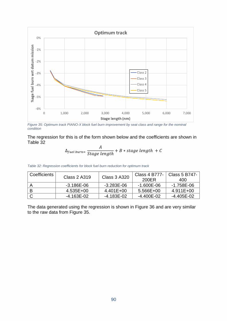
90

Figure 35: Optimum track PIANO-X block fuel burn improvement by seat class and range for the nominal condition

The regression for this is of the form shown below and the coefficients are shown in Table 32

∆𝑓𝑓𝑓𝑓𝑓𝑓𝑓𝑓 𝑏𝑏𝑓𝑓𝑏𝑏𝑏𝑏= 𝐴𝐴

𝑆𝑆𝑓𝑓𝑟𝑟𝑟𝑟𝑟𝑟 𝑙𝑙𝑟𝑟𝑙𝑙𝑟𝑟𝑓𝑓ℎ+ 𝐵𝐵 ∗ 𝑠𝑠𝑓𝑓𝑟𝑟𝑟𝑟𝑟𝑟 𝑙𝑙𝑟𝑟𝑙𝑙𝑟𝑟𝑓𝑓ℎ + 𝑆𝑆

Table 32: Regression coefficients for block fuel burn reduction for optimum track


Class 5 B747-400

A -3.186E-06 -3.283E-06 -1.600E-06 -1.758E-06 B 4.535E+00 4.401E+00 5.566E+00 4.911E+00 C -4.163E-02 -4.183E-02 -4.400E-02 -4.405E-02

The data generated using the regression is shown in Figure 36 and are very similar to the raw data from Figure 35.

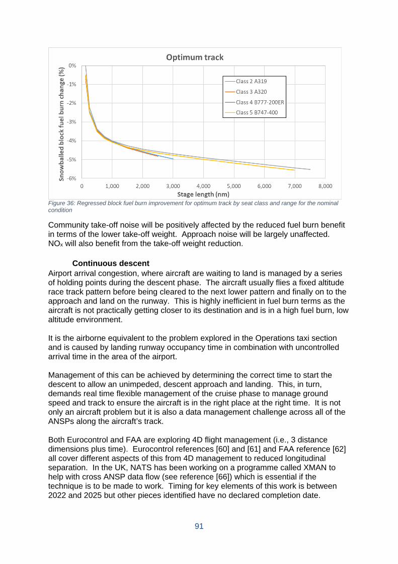
91

Figure 36: Regressed block fuel burn improvement for optimum track by seat class and range for the nominal condition

Community take-off noise will be positively affected by the reduced fuel burn benefit in terms of the lower take-off weight. Approach noise will be largely unaffected. NOx will also benefit from the take-off weight reduction.

Continuous descent Airport arrival congestion, where aircraft are waiting to land is managed by a series of holding points during the descent phase. The aircraft usually flies a fixed altitude race track pattern before being cleared to the next lower pattern and finally on to the approach and land on the runway. This is highly inefficient in fuel burn terms as the aircraft is not practically getting closer to its destination and is in a high fuel burn, low altitude environment. It is the airborne equivalent to the problem explored in the Operations taxi section and is caused by landing runway occupancy time in combination with uncontrolled arrival time in the area of the airport. Management of this can be achieved by determining the correct time to start the descent to allow an unimpeded, descent approach and landing. This, in turn, demands real time flexible management of the cruise phase to manage ground speed and track to ensure the aircraft is in the right place at the right time. It is not only an aircraft problem but it is also a data management challenge across all of the ANSPs along the aircraft’s track. Both Eurocontrol and FAA are exploring 4D flight management (i.e., 3 distance dimensions plus time). Eurocontrol references [60] and [61] and FAA reference [62] all cover different aspects of this from 4D management to reduced longitudinal separation. In the UK, NATS has been working on a programme called XMAN to help with cross ANSP data flow (see reference [66]) which is essential if the technique is to be made to work. Timing for key elements of this work is between 2022 and 2025 but other pieces identified have no declared completion date.

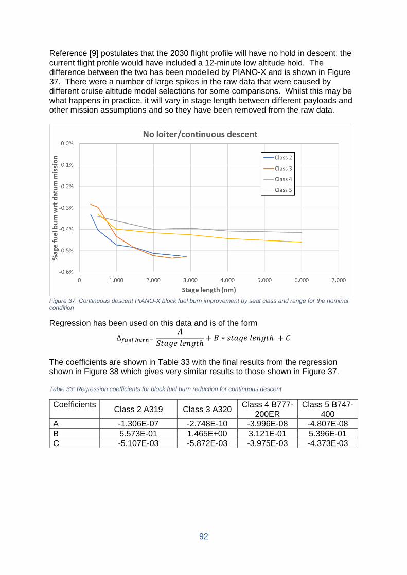
92

Reference [9] postulates that the 2030 flight profile will have no hold in descent; the current flight profile would have included a 12-minute low altitude hold. The difference between the two has been modelled by PIANO-X and is shown in Figure 37. There were a number of large spikes in the raw data that were caused by different cruise altitude model selections for some comparisons. Whilst this may be what happens in practice, it will vary in stage length between different payloads and other mission assumptions and so they have been removed from the raw data.

Figure 37: Continuous descent PIANO-X block fuel burn improvement by seat class and range for the nominal condition

Regression has been used on this data and is of the form



The coefficients are shown in Table 33 with the final results from the regression shown in Figure 38 which gives very similar results to those shown in Figure 37. Table 33: Regression coefficients for block fuel burn reduction for continuous descent


Class 5 B747-400

A -1.306E-07 -2.748E-10 -3.996E-08 -4.807E-08 B 5.573E-01 1.465E+00 3.121E-01 5.396E-01 C -5.107E-03 -5.872E-03 -3.975E-03 -4.373E-03

93

Figure 38: Regressed block fuel burn improvement for continuous descent by seat class and range for the nominal condition

The impact of this on community noise and local air quality is negligible given the tiny improvement in block fuel predicted. More practically however, removing holds over populated areas will reduce the noise and improve local air quality even if it isn’t part of the formal definition of community noise and local air quality.

Reduced contingency There are formal requirements that aircraft carry sufficient extra fuel to account for unforeseen circumstances en-route (see reference [3]). These can include stronger than forecast winds, longer than planned flight tracks and lower than planned cruise altitudes, all of which increase the amount of fuel burnt. This extra fuel is called contingency and is shown on the diagram in Figure 30 as a “5% flight fuel allowance”. The practice of carrying extra fuel causes more fuel to be burnt to carry it. Any reduction in the extra fuel carried will help reduce fuel burn. Greater robustness in forecasting and flight planning in terms of winds, routes and altitudes is the key to reducing the contingency carried. FAA reference [62] identifies data management systems and improved weather prediction capabilities as areas being worked on. The former project is due to be completed in 2025 but the latter one has no date; there is also no indication of any potential benefit. It is also clear that work required to deliver all of the other flight phase improvements cited above will support more robust flight planning. Reference [9] suggests that today’s assumption of a 5% contingency can be reduced to 3% by 2030. This has been used in the PIANO-X model and the raw data are shown in Figure 39.

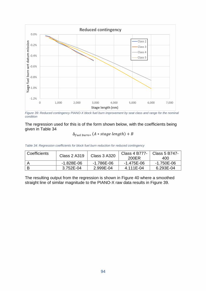
94

Figure 39: Reduced contingency PIANO-X block fuel burn improvement by seat class and range for the nominal condition

The regression used for this is of the form shown below, with the coefficients being given in Table 34

∆𝑓𝑓𝑓𝑓𝑓𝑓𝑓𝑓 𝑏𝑏𝑓𝑓𝑏𝑏𝑏𝑏= (𝐴𝐴 ∗ 𝑠𝑠𝑓𝑓𝑟𝑟𝑟𝑟𝑟𝑟 𝑙𝑙𝑟𝑟𝑙𝑙𝑟𝑟𝑓𝑓ℎ) + 𝐵𝐵

Table 34: Regression coefficients for block fuel burn reduction for reduced contingency


Class 5 B747-400

A -1.828E-06 -1.786E-06 -1.475E-06 -1.750E-06 B 3.752E-04 2.999E-04 4.111E-04 6.293E-04

The resulting output from the regression is shown in Figure 40 where a smoothed straight line of similar magnitude to the PIANO-X raw data results in Figure 39.

95

Figure 40: Regressed block fuel burn improvement for reduced contingency by seat class and range for the nominal condition

The impact of this on community noise and local air quality is negligible given the small improvement in block fuel predicted. It should be noted however, that the aircraft landing weight will be slightly lower given the reduction in fuel carried on a normal landing and so any benefits will accrue there as well as during take-off.

Reduced diversion hold Another key part of the reserve fuel philosophy is the diversion, where an aircraft carries sufficient fuel to fly to an alternative pre-specified destination in the event that the original destination is closed (through, for example, unexpected weather or a runway incident or accident). It is shown in Figure 30 as a notional distance of 200 nm to simulate the flight to the alternative destination and this part of the reserve is unlikely ever to be removed. What is open to improvement though, is the extra hold in preparation for landing at the alternative destination. It is included because the destination airport is not expecting all of the extra flights and gets congested so that it has to put aircraft in the hold prior to landing (in the same way as covered for continuous descent but more extreme). As noted above, the practice of carrying extra fuel causes more fuel to be burnt to carry it and so any reduction in the extra fuel carried will help reduce fuel burn. The solution is very similar to that section although has to be more flexible to manage the sudden emergence of a stream of diversions. The research comments from the continuous descent section are equally valid in this case. The difference is in the degree of change that can be anticipated. The NASA report, reference [9] points to reducing diversion hold time from 30 minutes to 10 minutes and this has been modelled in PIANO-X; the raw data are shown in Figure 41.

96

Figure 41: Reduced diversion hold PIANO-X block fuel burn improvement by seat class and range for the nominal condition

The resulting regression is of the following form with the relevant coefficients being given in Table 35.



Table 35:Regression coefficients for block fuel burn reduction for reduced diversion hold


Class 5 B747-400

A -4.741E-07 -8.019E-07 -5.672E-08 -1.251E-07 B 9.308E-01 1.119E+00 8.587E-01 1.037E+00 C -9.546E-03 -9.048E-03 -8.103E-03 -8.603E-03

The values created when using the regression are shown in Figure 42 and are a good representation of the PIANO-X raw data from Figure 41.

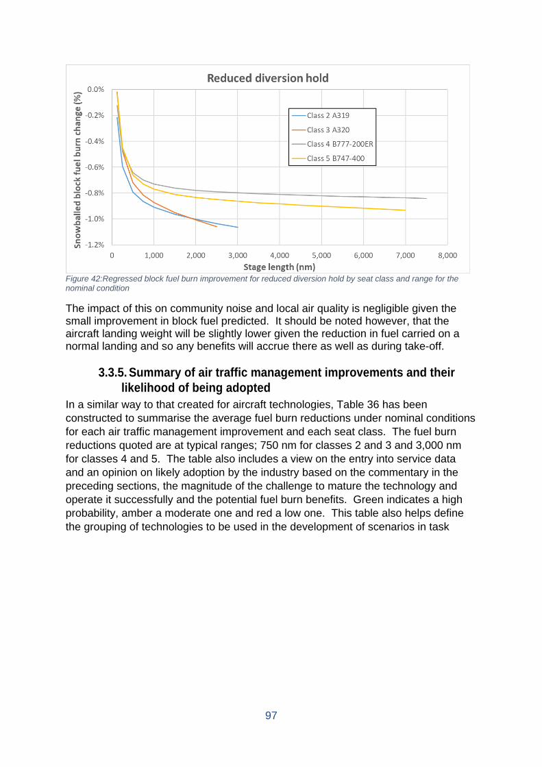
97

Figure 42:Regressed block fuel burn improvement for reduced diversion hold by seat class and range for the nominal condition

The impact of this on community noise and local air quality is negligible given the small improvement in block fuel predicted. It should be noted however, that the aircraft landing weight will be slightly lower given the reduction in fuel carried on a normal landing and so any benefits will accrue there as well as during take-off.

3.3.5. Summary of air traffic management improvements and their likelihood of being adopted

In a similar way to that created for aircraft technologies, Table 36 has been constructed to summarise the average fuel burn reductions under nominal conditions for each air traffic management improvement and each seat class. The fuel burn reductions quoted are at typical ranges; 750 nm for classes 2 and 3 and 3,000 nm for classes 4 and 5. The table also includes a view on the entry into service data and an opinion on likely adoption by the industry based on the commentary in the preceding sections, the magnitude of the challenge to mature the technology and operate it successfully and the potential fuel burn benefits. Green indicates a high probability, amber a moderate one and red a low one. This table also helps define the grouping of technologies to be used in the development of scenarios in task

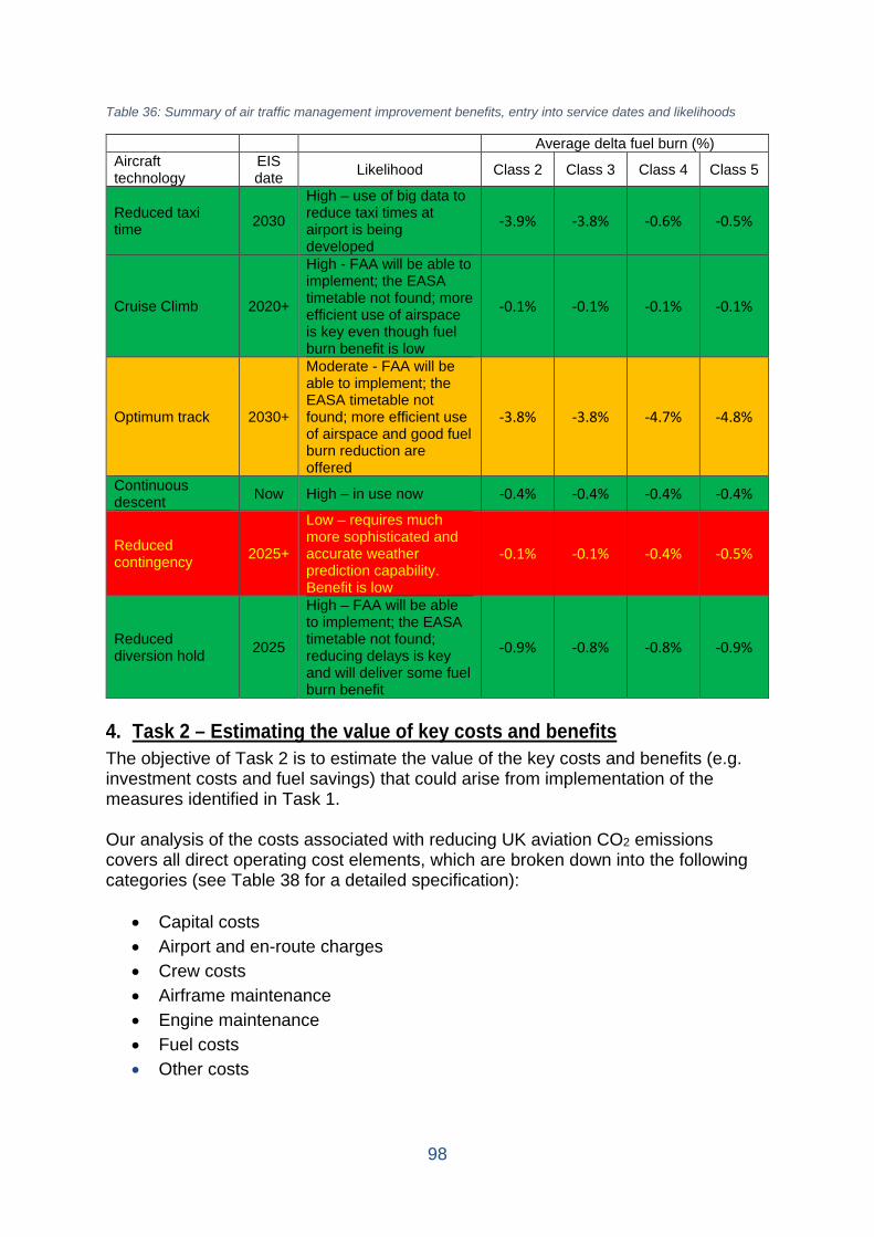
98

Table 36: Summary of air traffic management improvement benefits, entry into service dates and likelihoods


EIS date Likelihood Class 2 Class 3 Class 4 Class 5

Reduced taxi time 2030

High – use of big data to reduce taxi times at airport is being developed

-3.9% -3.8% -0.6% -0.5%

Cruise Climb 2020+

High - FAA will be able to implement; the EASA timetable not found; more efficient use of airspace is key even though fuel burn benefit is low

-0.1% -0.1% -0.1% -0.1%

Optimum track 2030+

Moderate - FAA will be able to implement; the EASA timetable not found; more efficient use of airspace and good fuel burn reduction are offered

-3.8% -3.8% -4.7% -4.8%

Continuous descent Now High – in use now -0.4% -0.4% -0.4% -0.4%

Reduced contingency 2025+

Low – requires much more sophisticated and accurate weather prediction capability. Benefit is low

-0.1% -0.1% -0.4% -0.5%

Reduced diversion hold 2025

High – FAA will be able to implement; the EASA timetable not found; reducing delays is key and will deliver some fuel burn benefit

-0.9% -0.8% -0.8% -0.9%

4. Task 2 – Estimating the value of key costs and benefits The objective of Task 2 is to estimate the value of the key costs and benefits (e.g. investment costs and fuel savings) that could arise from implementation of the measures identified in Task 1. Our analysis of the costs associated with reducing UK aviation CO2 emissions covers all direct operating cost elements, which are broken down into the following categories (see Table 38 for a detailed specification):

• Capital costs • Airport and en-route charges • Crew costs • Airframe maintenance • Engine maintenance • Fuel costs • Other costs

99

The capital cost estimates are based upon a cost model which is described in section 6.1. Most of the other cost elements were estimated with an econometric model, which is based upon various schedules from publicly available U.S. operations and cost data (US Form 41) in Reference [67] and explained in detail in section 4.2.

4.1. Aircraft Capital Costs Aircraft production costs are proprietary. With the exception of a few studies from the 1970s, no reliable cost estimates are available. Hence, this study relies on aircraft cost models. Aircraft cost estimation models are typically based upon statistical relationships from past aircraft programmes. (As such, they exclude research and technology costs). Perhaps the two most well-known cost models are those by Roskam (reference [68]) and the Development and Procurement Cost of Aircraft (DAPCA) model, originally developed at RAND and further improved by Raymer in reference [69]. Both models identify aircraft weight (empty or take-off weight), maximum aircraft speed, maximum engine thrust, and the number of aircraft produced as the key determinants of aircraft capital costs. The relationship between aircraft costs and aircraft weight, maximum aircraft speed and maximum engine thrust is direct, that is, an increase in any of these variables leads to an increase in aircraft capital costs. In contrast, the relationship between aircraft costs and the number of aircraft produced is indirect due technological learning and economies of scale. The weight dependence implies that heavier and thus larger aircraft experience higher capital costs, everything else equal. However, without adjusting for the share of light-weight materials, the weight-based approach could be misleading as it would project lower capital costs of a carbon fibre composite-intensive aircraft compared to a comparable metal-intensive aircraft, all other factors equal. Because only the enhanced DAPCA IV model allows for differences in material composition, it was chosen for this study. The DAPCA IV model, which is the most recent in a series of DAPCA cost models, estimates the non-recurring (research and technology) costs and the recurring (production) costs of airframes using statistical relationships for engineering, tooling, manufacturing, and quality control, and various material and component costs (see reference [69]). The key determinants of airframe development and manufacturing costs are aircraft empty weight, maximum cruise speed, and the number of aircraft produced. Costs for avionics and interior require an exogenous input. We assumed a typical production run of 500 aircraft. Because engine research and technology costs are excluded in the DAPCA model, Raymer provided cost estimation relationships for engine manufacturing costs depending on engine thrust, maximum Mach number, turbine inlet temperature, and production quantity in 2012 U.S. dollars. Partly because of the challenge of collecting turbine inlet temperatures for current and future engines, we developed a different engine cost model, which explains the engine list price as a function of maximum thrust, cruise engine specific fuel consumption, and certification year. We then applied a typical discount of 70% to arrive at the engine research and technology and production costs, which is based upon confidential discussions with industry experts. The engine list price model is specified as follows:

100

ln 𝐿𝐿𝐵𝐵_𝐸𝐸𝑙𝑙𝑟𝑟𝑡𝑡𝑙𝑙𝑟𝑟 = 𝛽𝛽0 + 𝛽𝛽1 ln𝑇𝑇𝑇𝑇𝑅𝑅 +𝛽𝛽2 ln 𝑆𝑆𝑍𝑍𝑆𝑆 + 𝛽𝛽3 CYR + 𝜀𝜀

The underlying data sources consist of the Airliner Price Guide in reference [70], which reports historical engine prices, maximum thrust levels, and some engine SFC data. The latter was complemented with historical data from Ellondee Ltd. Ellondee Ltd. also provided historical certification years. Table 37 reports the parameter estimates and t-statistics (in parenthesis), which were derived with OLS. As expected, the engine list price correlates directly with the maximum thrust and the certification year, and indirectly with specific fuel consumption. Table 37: Estimated Engine List Price Model

Number of Observations 71 Adjusted R2 0.9624 β0 Constant -34.08 (-8.65) β1 Total thrust THR 0.655 (21.2) β2 Engine specific fuel consumption SFC -0.696 (-2.23) β3 Certification year CYR 0.015 (7.48)

These parametric relationships produce plausible cost estimates. For example, applying the enhanced DAPCA IV model with our engine cost model yields production costs of $49.7 mln for the A320-200 aircraft. This value compares to the average aircraft price of $46.6 mln in 2012 from reference [70]. However, after subtracting $12.1 mln for non-recurring costs (as far more than 500 aircraft have been produced to date), the remaining recurring costs result in $39.3 mln, resulting in a 19% mark up. To account for the significantly larger amount of carbon fibre materials projected to be employed in future versions of single-aisle, narrow-body aircraft, we used an adjustment factor of 1.45 for the extra time dedicated to tooling, manufacturing, and quality control, which is the midpoint value of the range 1.1 to 1.8 given in reference [68]. Based upon a review of studies and news stories, we also added $(2012) 1,750 per seat for Class 2 and 3 aircraft and twice that amount for the Class 4 and 5 aircraft, due to the significantly more expensive business class seats, which is more prevalent in these vehicles. In addition, in line with FAA estimates (see reference [71]), we added $670k per aircraft to be compliant with advanced air traffic management procedures (see Section 3.3). We annualized the capital costs using a residual value of 10% and an economic lifetime of 20 years following a linear depreciation. Interest on the investment was assumed to be 4%/yr and insurance to be 0.5%/yr (reference [13]).

4.2. Other Operating Cost Elements The method employed for estimating operating cost components other than capital costs essentially follows the work by Harris, reference [72]. Table 38 reports the composition of DOC components and the respective reporting schedule from the US Form 41 entries. The top 10 airlines (Alaska, American, Delta, Hawaiian, Jet Blue, Skywest, Southwest, United, US Air, Virgin) were analysed, jointly accounting for 85% of domestic RPK. Only domestic travel is considered.

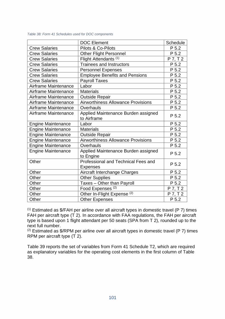
101

Table 38: Form 41 Schedules used for DOC components

DOC Element Schedule Crew Salaries Pilots & Co-Pilots P 5.2 Crew Salaries Other Flight Personnel P 5.2 Crew Salaries Flight Attendants (1) P 7, T 2 Crew Salaries Trainees and Instructors P 5.2 Crew Salaries Personnel Expenses P 5.2 Crew Salaries Employee Benefits and Pensions P 5.2 Crew Salaries Payroll Taxes P 5.2 Airframe Maintenance Labor P 5.2 Airframe Maintenance Materials P 5.2 Airframe Maintenance Outside Repair P 5.2 Airframe Maintenance Airworthiness Allowance Provisions P 5.2 Airframe Maintenance Overhauls P 5.2 Airframe Maintenance Applied Maintenance Burden assigned

to Airframe P 5.2

Engine Maintenance Labor P 5.2 Engine Maintenance Materials P 5.2 Engine Maintenance Outside Repair P 5.2 Engine Maintenance Airworthiness Allowance Provisions P 5.2 Engine Maintenance Overhauls P 5.2 Engine Maintenance Applied Maintenance Burden assigned

to Engine P 5.2

Other Professional and Technical Fees and Expenses P 5.2

Other Aircraft Interchange Charges P 5.2 Other Other Supplies P 5.2 Other Taxes – Other than Payroll P 5.2 Other Food Expenses (2) P 7, T 2 Other Other In-Flight Expense (2) P 7, T 2 Other Other Expenses P 5.2

(1) Estimated as $/FAH per airline over all aircraft types in domestic travel (P 7) times FAH per aircraft type (T 2). In accordance with FAA regulations, the FAH per aircraft type is based upon 1 flight attendant per 50 seats (SPA from T 2), rounded up to the next full number. (2) Estimated as $/RPM per airline over all aircraft types in domestic travel (P 7) times RPM per aircraft type (T 2). Table 39 reports the set of variables from Form 41 Schedule T2, which are required as explanatory variables for the operating cost elements in the first column of Table 38.

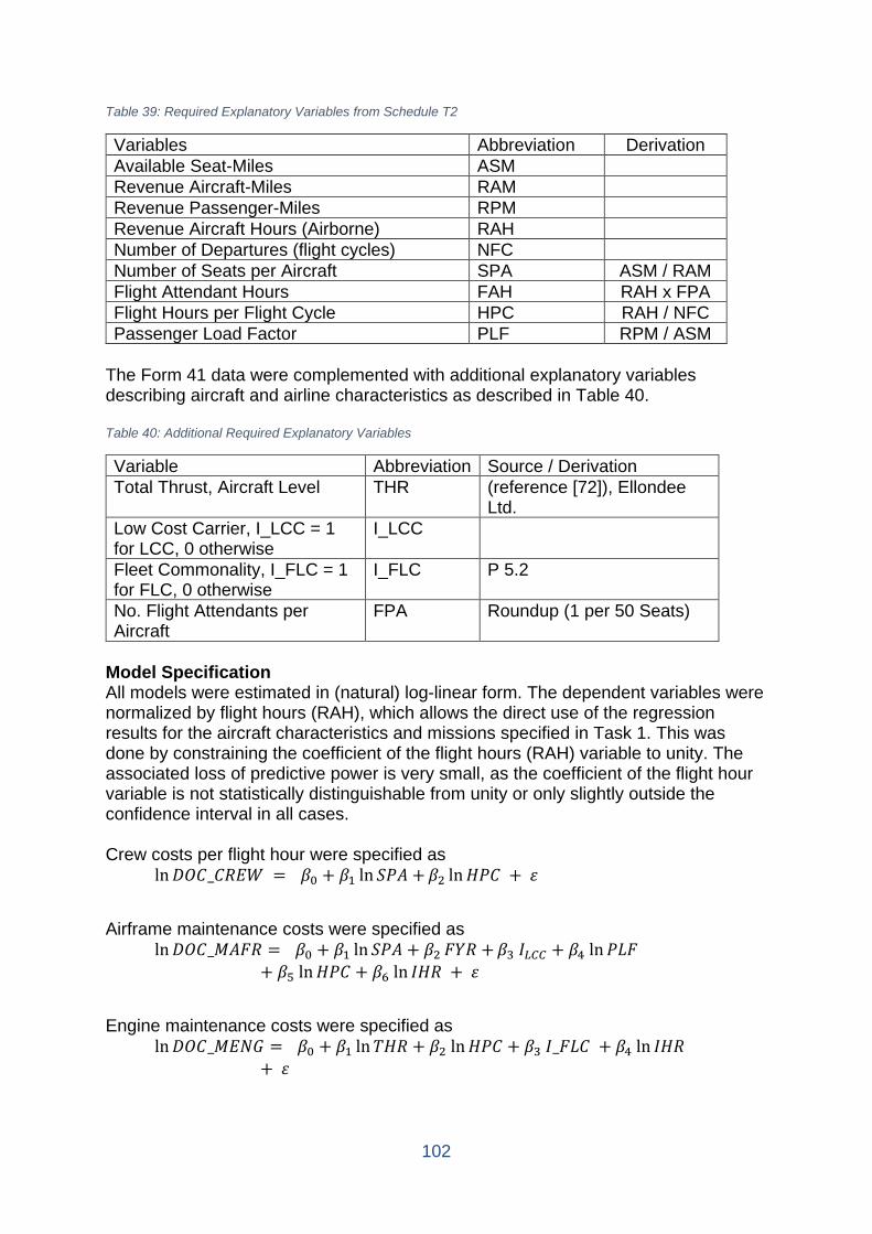
102

Table 39: Required Explanatory Variables from Schedule T2

Variables Abbreviation Derivation Available Seat-Miles ASM Revenue Aircraft-Miles RAM Revenue Passenger-Miles RPM Revenue Aircraft Hours (Airborne) RAH Number of Departures (flight cycles) NFC Number of Seats per Aircraft SPA ASM / RAM Flight Attendant Hours FAH RAH x FPA Flight Hours per Flight Cycle HPC RAH / NFC Passenger Load Factor PLF RPM / ASM

The Form 41 data were complemented with additional explanatory variables describing aircraft and airline characteristics as described in Table 40. Table 40: Additional Required Explanatory Variables

Variable Abbreviation Source / Derivation Total Thrust, Aircraft Level THR (reference [72]), Ellondee

Ltd. Low Cost Carrier, I_LCC = 1 for LCC, 0 otherwise

I_LCC

Fleet Commonality, I_FLC = 1 for FLC, 0 otherwise

I_FLC P 5.2

No. Flight Attendants per Aircraft

FPA Roundup (1 per 50 Seats)

Model Specification All models were estimated in (natural) log-linear form. The dependent variables were normalized by flight hours (RAH), which allows the direct use of the regression results for the aircraft characteristics and missions specified in Task 1. This was done by constraining the coefficient of the flight hours (RAH) variable to unity. The associated loss of predictive power is very small, as the coefficient of the flight hour variable is not statistically distinguishable from unity or only slightly outside the confidence interval in all cases. Crew costs per flight hour were specified as ln𝐷𝐷𝑇𝑇𝑆𝑆_𝑆𝑆𝑅𝑅𝐸𝐸𝑇𝑇 = 𝛽𝛽0 + 𝛽𝛽1 ln 𝑆𝑆𝐵𝐵𝐴𝐴 +𝛽𝛽2 ln𝑇𝑇𝐵𝐵𝑆𝑆 + 𝜀𝜀

Airframe maintenance costs were specified as ln𝐷𝐷𝑇𝑇𝑆𝑆_𝑀𝑀𝐴𝐴𝑍𝑍𝑅𝑅 = 𝛽𝛽0 + 𝛽𝛽1 ln 𝑆𝑆𝐵𝐵𝐴𝐴 + 𝛽𝛽2 𝑍𝑍𝐹𝐹𝑅𝑅 +𝛽𝛽3 𝐼𝐼𝐿𝐿𝐶𝐶𝐶𝐶 + 𝛽𝛽4 ln𝐵𝐵𝐿𝐿𝑍𝑍

+ 𝛽𝛽5 ln𝑇𝑇𝐵𝐵𝑆𝑆 + 𝛽𝛽6 ln 𝐼𝐼𝑇𝑇𝑅𝑅 + 𝜀𝜀

Engine maintenance costs were specified as ln𝐷𝐷𝑇𝑇𝑆𝑆_𝑀𝑀𝐸𝐸𝑀𝑀𝑀𝑀 = 𝛽𝛽0 + 𝛽𝛽1 ln𝑇𝑇𝑇𝑇𝑅𝑅 + 𝛽𝛽2 ln𝑇𝑇𝐵𝐵𝑆𝑆 + 𝛽𝛽3 𝐼𝐼_𝑍𝑍𝐿𝐿𝑆𝑆 + 𝛽𝛽4 ln 𝐼𝐼𝑇𝑇𝑅𝑅

+ 𝜀𝜀

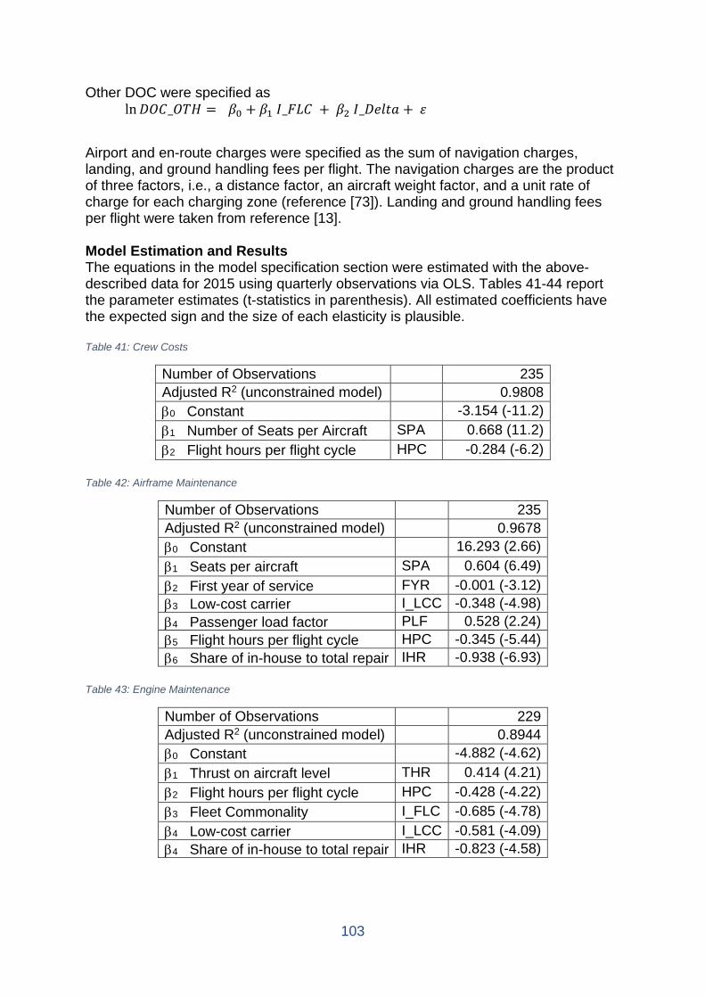
103

Other DOC were specified as ln𝐷𝐷𝑇𝑇𝑆𝑆_𝑇𝑇𝑇𝑇𝑇𝑇 = 𝛽𝛽0 + 𝛽𝛽1 𝐼𝐼_𝑍𝑍𝐿𝐿𝑆𝑆 + 𝛽𝛽2 𝐼𝐼_𝐷𝐷𝑟𝑟𝑙𝑙𝑓𝑓𝑟𝑟 + 𝜀𝜀

Airport and en-route charges were specified as the sum of navigation charges, landing, and ground handling fees per flight. The navigation charges are the product of three factors, i.e., a distance factor, an aircraft weight factor, and a unit rate of charge for each charging zone (reference [73]). Landing and ground handling fees per flight were taken from reference [13]. Model Estimation and Results The equations in the model specification section were estimated with the above-described data for 2015 using quarterly observations via OLS. Tables 41-44 report the parameter estimates (t-statistics in parenthesis). All estimated coefficients have the expected sign and the size of each elasticity is plausible. Table 41: Crew Costs

Number of Observations 235 Adjusted R2 (unconstrained model) 0.9808 β0 Constant -3.154 (-11.2) β1 Number of Seats per Aircraft SPA 0.668 (11.2) β2 Flight hours per flight cycle HPC -0.284 (-6.2)

Table 42: Airframe Maintenance

Number of Observations 235 Adjusted R2 (unconstrained model) 0.9678 β0 Constant 16.293 (2.66) β1 Seats per aircraft SPA 0.604 (6.49) β2 First year of service FYR -0.001 (-3.12) β3 Low-cost carrier I_LCC -0.348 (-4.98) β4 Passenger load factor PLF 0.528 (2.24) β5 Flight hours per flight cycle HPC -0.345 (-5.44) β6 Share of in-house to total repair IHR -0.938 (-6.93)

Table 43: Engine Maintenance

Number of Observations 229 Adjusted R2 (unconstrained model) 0.8944 β0 Constant -4.882 (-4.62) β1 Thrust on aircraft level THR 0.414 (4.21) β2 Flight hours per flight cycle HPC -0.428 (-4.22) β3 Fleet Commonality I_FLC -0.685 (-4.78) β4 Low-cost carrier I_LCC -0.581 (-4.09) β4 Share of in-house to total repair IHR -0.823 (-4.58)

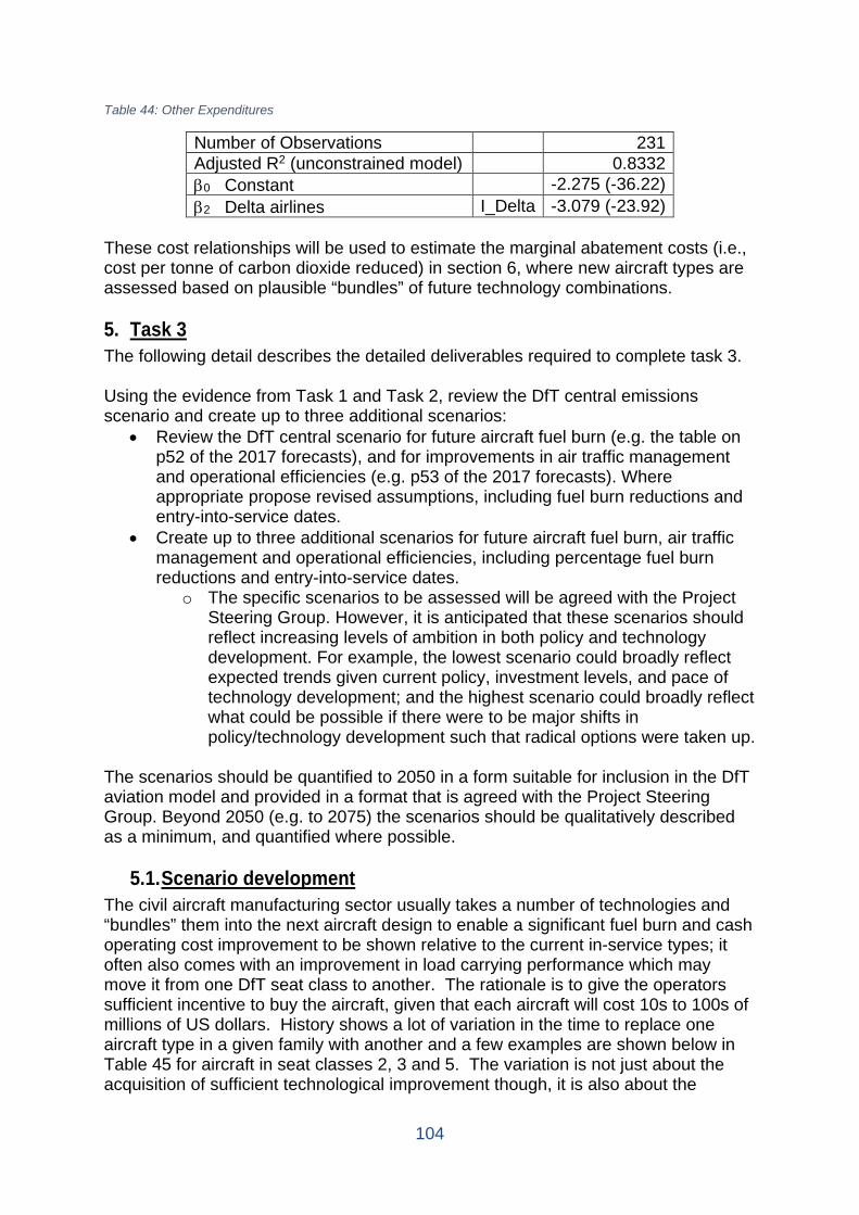
104

Table 44: Other Expenditures

Number of Observations 231 Adjusted R2 (unconstrained model) 0.8332 β0 Constant -2.275 (-36.22) β2 Delta airlines I_Delta -3.079 (-23.92)

These cost relationships will be used to estimate the marginal abatement costs (i.e., cost per tonne of carbon dioxide reduced) in section 6, where new aircraft types are assessed based on plausible “bundles” of future technology combinations. 5. Task 3 The following detail describes the detailed deliverables required to complete task 3. Using the evidence from Task 1 and Task 2, review the DfT central emissions scenario and create up to three additional scenarios:

• Review the DfT central scenario for future aircraft fuel burn (e.g. the table on p52 of the 2017 forecasts), and for improvements in air traffic management and operational efficiencies (e.g. p53 of the 2017 forecasts). Where appropriate propose revised assumptions, including fuel burn reductions and entry-into-service dates.

• Create up to three additional scenarios for future aircraft fuel burn, air traffic management and operational efficiencies, including percentage fuel burn reductions and entry-into-service dates.

o The specific scenarios to be assessed will be agreed with the Project Steering Group. However, it is anticipated that these scenarios should reflect increasing levels of ambition in both policy and technology development. For example, the lowest scenario could broadly reflect expected trends given current policy, investment levels, and pace of technology development; and the highest scenario could broadly reflect what could be possible if there were to be major shifts in policy/technology development such that radical options were taken up.

The scenarios should be quantified to 2050 in a form suitable for inclusion in the DfT aviation model and provided in a format that is agreed with the Project Steering Group. Beyond 2050 (e.g. to 2075) the scenarios should be qualitatively described as a minimum, and quantified where possible.

5.1. Scenario development The civil aircraft manufacturing sector usually takes a number of technologies and “bundles” them into the next aircraft design to enable a significant fuel burn and cash operating cost improvement to be shown relative to the current in-service types; it often also comes with an improvement in load carrying performance which may move it from one DfT seat class to another. The rationale is to give the operators sufficient incentive to buy the aircraft, given that each aircraft will cost 10s to 100s of millions of US dollars. History shows a lot of variation in the time to replace one aircraft type in a given family with another and a few examples are shown below in Table 45 for aircraft in seat classes 2, 3 and 5. The variation is not just about the acquisition of sufficient technological improvement though, it is also about the

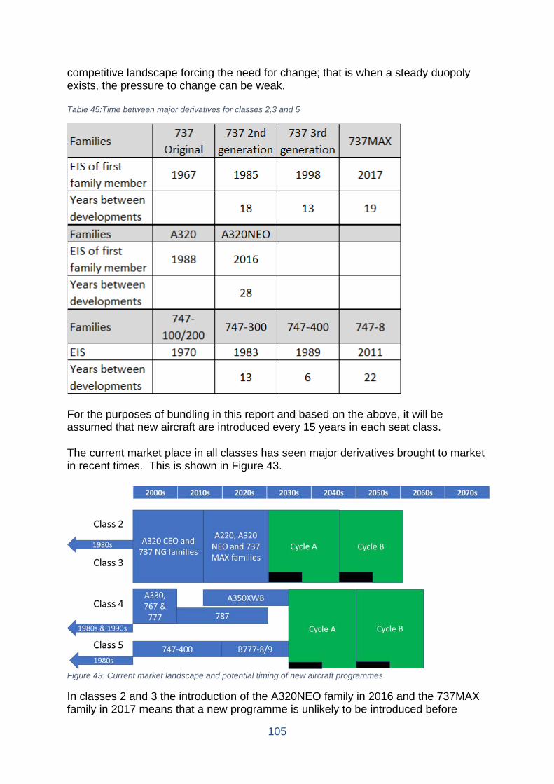
105

competitive landscape forcing the need for change; that is when a steady duopoly exists, the pressure to change can be weak. Table 45:Time between major derivatives for classes 2,3 and 5

For the purposes of bundling in this report and based on the above, it will be assumed that new aircraft are introduced every 15 years in each seat class. The current market place in all classes has seen major derivatives brought to market in recent times. This is shown in Figure 43.

Figure 43: Current market landscape and potential timing of new aircraft programmes

In classes 2 and 3 the introduction of the A320NEO family in 2016 and the 737MAX family in 2017 means that a new programme is unlikely to be introduced before

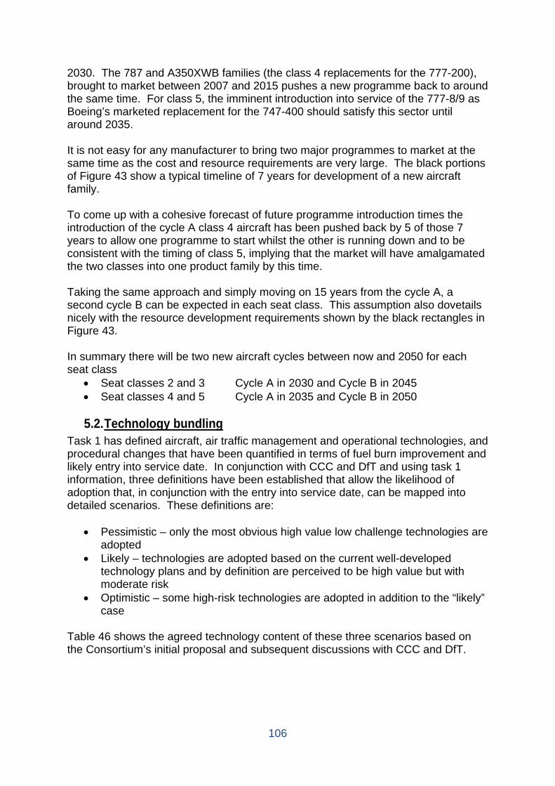
106

2030. The 787 and A350XWB families (the class 4 replacements for the 777-200), brought to market between 2007 and 2015 pushes a new programme back to around the same time. For class 5, the imminent introduction into service of the 777-8/9 as Boeing’s marketed replacement for the 747-400 should satisfy this sector until around 2035. It is not easy for any manufacturer to bring two major programmes to market at the same time as the cost and resource requirements are very large. The black portions of Figure 43 show a typical timeline of 7 years for development of a new aircraft family. To come up with a cohesive forecast of future programme introduction times the introduction of the cycle A class 4 aircraft has been pushed back by 5 of those 7 years to allow one programme to start whilst the other is running down and to be consistent with the timing of class 5, implying that the market will have amalgamated the two classes into one product family by this time. Taking the same approach and simply moving on 15 years from the cycle A, a second cycle B can be expected in each seat class. This assumption also dovetails nicely with the resource development requirements shown by the black rectangles in Figure 43. In summary there will be two new aircraft cycles between now and 2050 for each seat class

• Seat classes 2 and 3 Cycle A in 2030 and Cycle B in 2045 • Seat classes 4 and 5 Cycle A in 2035 and Cycle B in 2050

5.2. Technology bundling

Task 1 has defined aircraft, air traffic management and operational technologies, and procedural changes that have been quantified in terms of fuel burn improvement and likely entry into service date. In conjunction with CCC and DfT and using task 1 information, three definitions have been established that allow the likelihood of adoption that, in conjunction with the entry into service date, can be mapped into detailed scenarios. These definitions are:

• Pessimistic – only the most obvious high value low challenge technologies are adopted

• Likely – technologies are adopted based on the current well-developed technology plans and by definition are perceived to be high value but with moderate risk

• Optimistic – some high-risk technologies are adopted in addition to the “likely” case

Table 46 shows the agreed technology content of these three scenarios based on the Consortium’s initial proposal and subsequent discussions with CCC and DfT.

107

Table 46: Technology implementation table for the three scenarios

The table breaks out the aircraft, operations and ATM elements separately and shows the degree of adoption by technology, technique or process in either the first (2030-2035) or second (2045-2050) new aircraft development cycle. Where possible mutually exclusive technologies have been removed to ensure that double accounting of fuel burn improvement is avoided.

5.2.1. Aircraft The 50% embodiment for ultra-high by-pass ratio turbofan and 15 aspect ratio wings in 2030-2035 has been applied because it is not expected that every new design will feature the technology in that time; the 100% by 2045-2050 means that all new aircraft designs will be using the technology by the later date. Open rotor is not expected in any scenario because the level of fuel burn improvement predicted for the ultra-high by-pass ratio engine is nearly as good as the open rotor and there doesn’t appear to be a compelling case to deploy resources for a small incremental improvement. Natural laminar flow is not expected in any scenario because hybrid laminar flow offers greater benefit and if the challenges for introduction can be overcome, that are common to both, then hybrid laminar flow will be the better solution. All-electric aircraft may be applicable to smaller aircraft in class 2 but is more likely to appear in a third aircraft iteration after 2050 and so is not part of these scenarios.

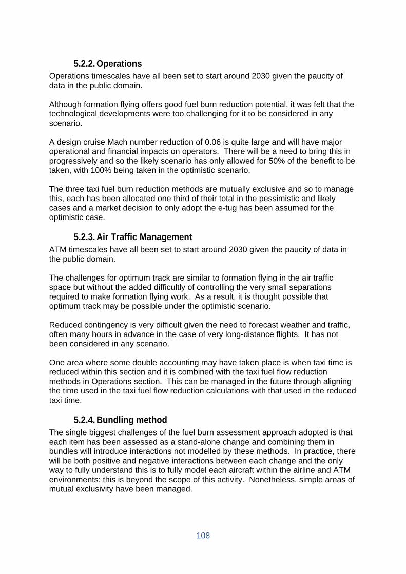
108

5.2.2. Operations

Operations timescales have all been set to start around 2030 given the paucity of data in the public domain. Although formation flying offers good fuel burn reduction potential, it was felt that the technological developments were too challenging for it to be considered in any scenario. A design cruise Mach number reduction of 0.06 is quite large and will have major operational and financial impacts on operators. There will be a need to bring this in progressively and so the likely scenario has only allowed for 50% of the benefit to be taken, with 100% being taken in the optimistic scenario. The three taxi fuel burn reduction methods are mutually exclusive and so to manage this, each has been allocated one third of their total in the pessimistic and likely cases and a market decision to only adopt the e-tug has been assumed for the optimistic case.

5.2.3. Air Traffic Management ATM timescales have all been set to start around 2030 given the paucity of data in the public domain. The challenges for optimum track are similar to formation flying in the air traffic space but without the added difficultly of controlling the very small separations required to make formation flying work. As a result, it is thought possible that optimum track may be possible under the optimistic scenario. Reduced contingency is very difficult given the need to forecast weather and traffic, often many hours in advance in the case of very long-distance flights. It has not been considered in any scenario. One area where some double accounting may have taken place is when taxi time is reduced within this section and it is combined with the taxi fuel flow reduction methods in Operations section. This can be managed in the future through aligning the time used in the taxi fuel flow reduction calculations with that used in the reduced taxi time.

5.2.4. Bundling method The single biggest challenges of the fuel burn assessment approach adopted is that each item has been assessed as a stand-alone change and combining them in bundles will introduce interactions not modelled by these methods. In practice, there will be both positive and negative interactions between each change and the only way to fully understand this is to fully model each aircraft within the airline and ATM environments: this is beyond the scope of this activity. Nonetheless, simple areas of mutual exclusivity have been managed.

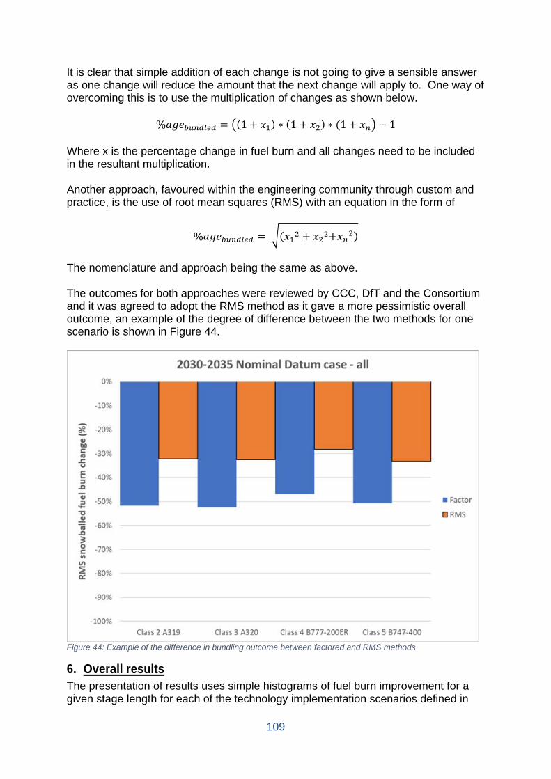
109

It is clear that simple addition of each change is not going to give a sensible answer as one change will reduce the amount that the next change will apply to. One way of overcoming this is to use the multiplication of changes as shown below.

%𝑟𝑟𝑟𝑟𝑟𝑟𝑏𝑏𝑓𝑓𝑏𝑏𝑏𝑏𝑓𝑓𝑓𝑓𝑏𝑏 = �(1 + 𝑡𝑡1) ∗ (1 + 𝑡𝑡2) ∗ (1 + 𝑡𝑡𝑏𝑏� − 1 Where x is the percentage change in fuel burn and all changes need to be included in the resultant multiplication. Another approach, favoured within the engineering community through custom and practice, is the use of root mean squares (RMS) with an equation in the form of

%𝑟𝑟𝑟𝑟𝑟𝑟𝑏𝑏𝑓𝑓𝑏𝑏𝑏𝑏𝑓𝑓𝑓𝑓𝑏𝑏 = �(𝑡𝑡12 + 𝑡𝑡22+𝑡𝑡𝑏𝑏2) The nomenclature and approach being the same as above. The outcomes for both approaches were reviewed by CCC, DfT and the Consortium and it was agreed to adopt the RMS method as it gave a more pessimistic overall outcome, an example of the degree of difference between the two methods for one scenario is shown in Figure 44.

Figure 44: Example of the difference in bundling outcome between factored and RMS methods

6. Overall results The presentation of results uses simple histograms of fuel burn improvement for a given stage length for each of the technology implementation scenarios defined in

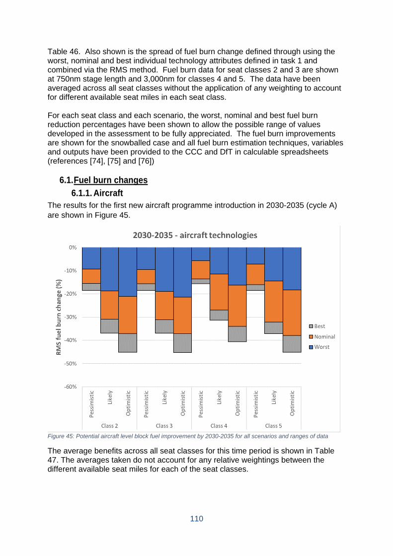
110

Table 46. Also shown is the spread of fuel burn change defined through using the worst, nominal and best individual technology attributes defined in task 1 and combined via the RMS method. Fuel burn data for seat classes 2 and 3 are shown at 750nm stage length and 3,000nm for classes 4 and 5. The data have been averaged across all seat classes without the application of any weighting to account for different available seat miles in each seat class. For each seat class and each scenario, the worst, nominal and best fuel burn reduction percentages have been shown to allow the possible range of values developed in the assessment to be fully appreciated. The fuel burn improvements are shown for the snowballed case and all fuel burn estimation techniques, variables and outputs have been provided to the CCC and DfT in calculable spreadsheets (references [74], [75] and [76])

6.1. Fuel burn changes 6.1.1. Aircraft

The results for the first new aircraft programme introduction in 2030-2035 (cycle A) are shown in Figure 45.

Figure 45: Potential aircraft level block fuel improvement by 2030-2035 for all scenarios and ranges of data

The average benefits across all seat classes for this time period is shown in Table 47. The averages taken do not account for any relative weightings between the different available seat miles for each of the seat classes.

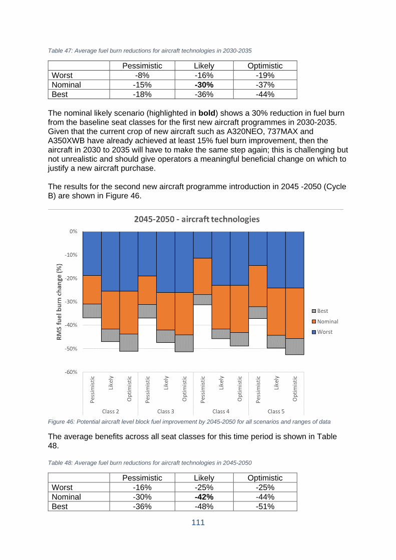
111

Table 47: Average fuel burn reductions for aircraft technologies in 2030-2035

Pessimistic Likely Optimistic Worst -8% -16% -19% Nominal -15% -30% -37% Best -18% -36% -44%

The nominal likely scenario (highlighted in bold) shows a 30% reduction in fuel burn from the baseline seat classes for the first new aircraft programmes in 2030-2035. Given that the current crop of new aircraft such as A320NEO, 737MAX and A350XWB have already achieved at least 15% fuel burn improvement, then the aircraft in 2030 to 2035 will have to make the same step again; this is challenging but not unrealistic and should give operators a meaningful beneficial change on which to justify a new aircraft purchase. The results for the second new aircraft programme introduction in 2045 -2050 (Cycle B) are shown in Figure 46.

Figure 46: Potential aircraft level block fuel improvement by 2045-2050 for all scenarios and ranges of data

The average benefits across all seat classes for this time period is shown in Table 48. Table 48: Average fuel burn reductions for aircraft technologies in 2045-2050


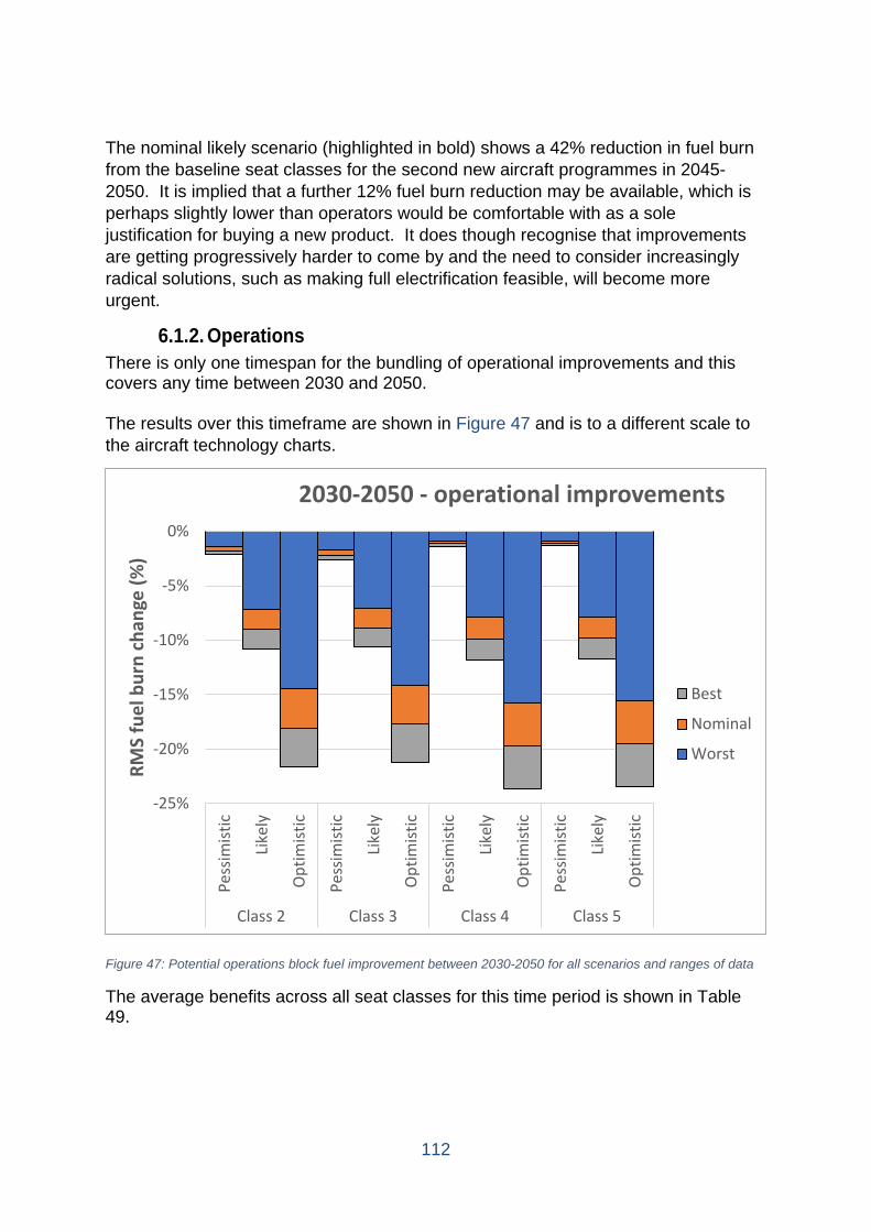
112

The nominal likely scenario (highlighted in bold) shows a 42% reduction in fuel burn from the baseline seat classes for the second new aircraft programmes in 2045-2050. It is implied that a further 12% fuel burn reduction may be available, which is perhaps slightly lower than operators would be comfortable with as a sole justification for buying a new product. It does though recognise that improvements are getting progressively harder to come by and the need to consider increasingly radical solutions, such as making full electrification feasible, will become more urgent.

6.1.2. Operations There is only one timespan for the bundling of operational improvements and this covers any time between 2030 and 2050. The results over this timeframe are shown in Figure 47 and is to a different scale to the aircraft technology charts.

Figure 47: Potential operations block fuel improvement between 2030-2050 for all scenarios and ranges of data

The average benefits across all seat classes for this time period is shown in Table 49.

-25%

-20%

-15%

-10%

-5%

0%

Pess

imist

ic

Like

ly

Opt

imist

ic

Pess

imist

ic

Like

ly

Opt

imist

ic

Pess

imist

ic

Like

ly

Opt

imist

ic

Pess

imist

ic

Like

ly

Opt

imist

ic


RMS

fuel

bur

n ch

ange

(%)

2030-2050 - operational improvements

Best

Nominal

Worst

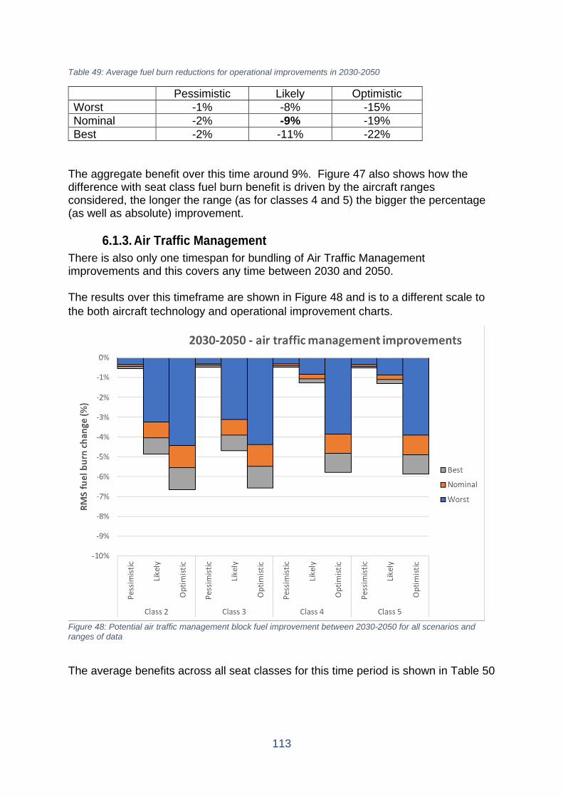
113

Table 49: Average fuel burn reductions for operational improvements in 2030-2050


The aggregate benefit over this time around 9%. Figure 47 also shows how the difference with seat class fuel burn benefit is driven by the aircraft ranges considered, the longer the range (as for classes 4 and 5) the bigger the percentage (as well as absolute) improvement.

6.1.3. Air Traffic Management There is also only one timespan for bundling of Air Traffic Management improvements and this covers any time between 2030 and 2050. The results over this timeframe are shown in Figure 48 and is to a different scale to the both aircraft technology and operational improvement charts.

Figure 48: Potential air traffic management block fuel improvement between 2030-2050 for all scenarios and ranges of data

The average benefits across all seat classes for this time period is shown in Table 50

114

Table 50: Average fuel burn reductions for air traffic management improvements in 2030-2050

Pessimistic Likely Optimistic Worst -0.3% -2.0% -4.1% Nominal -0.4% -2.5% -5.2% Best -0.5% -3.0% -6.2%

The aggregate benefit over this time is around 2.5%. The difference with seat class fuel burn benefit (shown in Figure 48) is driven by the inverse of aircraft ranges modelled, the longer the range (as for classes 4 and 5) the smaller the percentage improvement. This is because many ATM improvements are fixed values and so as the absolute fuel burn gets higher the percentage benefit gets lower.

6.1.4. All elements combined The RMS bundling method has also been used to bring together the aircraft technologies, operations and air traffic management improvement scenarios together to show the total system level potential benefit. The presentation style is the same as used for the Aircraft, Operations an ATM fuel burn improvements and the same stage lengths have been used. The results for the first new aircraft programme introduction in 2030-2035 combined with the single operations and air traffic management improvement levels are shown in Figure 49. The axis scale is the same as used for the aircraft technologies charts.

Figure 49: Potential combined block fuel improvement between 2030-2035 for all scenarios and ranges of data

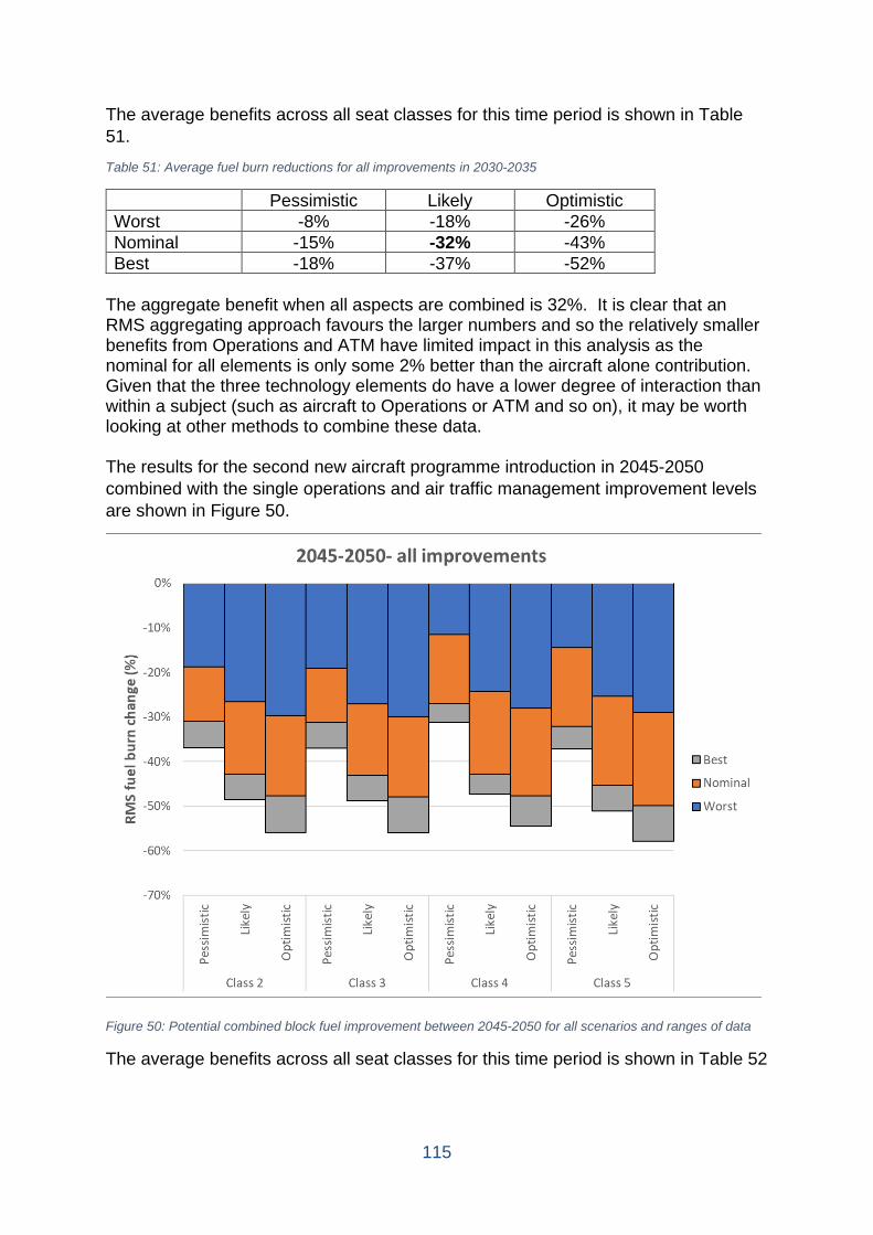
115

The average benefits across all seat classes for this time period is shown in Table 51. Table 51: Average fuel burn reductions for all improvements in 2030-2035


The aggregate benefit when all aspects are combined is 32%. It is clear that an RMS aggregating approach favours the larger numbers and so the relatively smaller benefits from Operations and ATM have limited impact in this analysis as the nominal for all elements is only some 2% better than the aircraft alone contribution. Given that the three technology elements do have a lower degree of interaction than within a subject (such as aircraft to Operations or ATM and so on), it may be worth looking at other methods to combine these data. The results for the second new aircraft programme introduction in 2045-2050 combined with the single operations and air traffic management improvement levels are shown in Figure 50.

Figure 50: Potential combined block fuel improvement between 2045-2050 for all scenarios and ranges of data

The average benefits across all seat classes for this time period is shown in Table 52

116

Table 52: Average fuel burn reductions for all improvements in 2045-2050


The average results for the overall scenario between 2045 and 2050 shown a nominal improvement of 44%. The increment relative to aircraft alone in the same timeframe is only 1% in this case and for the same reasons as described above with the added difficulty that there is no magnitude change in the Operations and Air Traffic Management outcomes between the two new aircraft introduction timeframes whereas the aircraft values increase significantly between the first and second new aircraft introductions.

6.1.5. Cost implications The estimated DOC by category from section 4 for the reference aircraft and those of the projected aircraft in 2030-2035 and 2045-2050 are shown in Tables 53-55 for the worst, nominal and best case for the likely scenario. US$(2012) were converted into £(2015) via a multiplier of 0.66 based upon the IMF International Financial Statistics Yearbook. The entries for capital costs, airport & en-route charges, crew costs, airframe and engine maintenance and other costs were derived as described in the Task 2 section. The fuel costs are based upon the projected aircraft fuel burn and a fuel price of £(2015) 1.3/Gal. No carbon price has been applied. As can be seen from Tables 53-55, the DOC in £ (2015) of all future designs in all scenarios are projected to be below those of the reference aircraft, irrespective of the scenario. The decline is the result of two contrasting trends:

• An increase in capital costs due to the more expensive fuel-saving technology employed

• A simultaneous, stronger decline in other operating cost components, predominantly fuel costs due to the projected higher fuel efficiency of future designs.

In addition, the aircraft weight-dependent airport & en-route charges are also expected to slightly decline due to the projected lower aircraft weight. Similarly, airframe maintenance is projected to decline, mainly because of a time trend of -0.1%/yr (Table 42) and engine maintenance is projected to be lower because of the lower thrust levels required for lighter-weight aircraft.

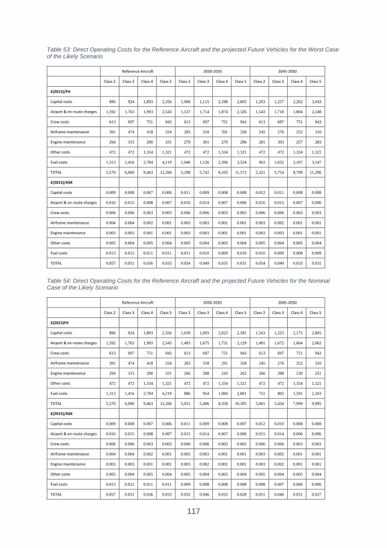
117

Table 53: Direct Operating Costs for the Reference Aircraft and the projected Future Vehicles for the Worst Case of the Likely Scenario

Reference Aircraft 2030-2035 2045-2050

Class 2 Class 3 Class 4 Class 5 Class 2 Class 3 Class 4 Class 5 Class 2 Class 3 Class 4 Class 5

£(2015)/FH

Capital costs 896 924 1,893 2,356 1,068 1,115 2,188 2,805 1,203 1,257 2,202 3,043

Airport & en-route charges 1,592 1,763 1,993 2,543 1,537 1,714 1,874 2,326 1,543 1,718 1,804 2,248

Crew costs 613 697 751 943 613 697 751 943 613 697 751 943

Airframe maintenance 391 474 418 554 283 318 291 358 245 276 252 310

Engine maintenance 294 315 290 331 279 301 270 296 281 303 257 283

Other costs 472 472 1,334 1,321 472 472 1,334 1,321 472 472 1,334 1,321

Fuel costs 1,313 1,416 2,784 4,219 1,046 1,126 2,396 3,524 963 1,032 2,107 3,147

TOTAL 5,570 6,060 9,463 12,266 5,298 5,742 9,105 11,572 5,321 5,754 8,709 11,296

£(2015)/ASK

Capital costs 0.009 0.008 0.007 0.006 0.011 0.009 0.008 0.008 0.012 0.011 0.008 0.008

Airport & en-route charges 0.016 0.015 0.008 0.007 0.016 0.014 0.007 0.006 0.016 0.015 0.007 0.006

Crew costs 0.006 0.006 0.003 0.003 0.006 0.006 0.003 0.003 0.006 0.006 0.003 0.003

Airframe maintenance 0.004 0.004 0.002 0.001 0.003 0.003 0.001 0.001 0.003 0.002 0.001 0.001

Engine maintenance 0.003 0.003 0.001 0.001 0.003 0.003 0.001 0.001 0.003 0.003 0.001 0.001

Other costs 0.005 0.004 0.005 0.004 0.005 0.004 0.005 0.004 0.005 0.004 0.005 0.004

Fuel costs 0.013 0.012 0.011 0.011 0.011 0.010 0.009 0.010 0.010 0.009 0.008 0.009

TOTAL 0.057 0.051 0.036 0.033 0.054 0.049 0.035 0.031 0.054 0.049 0.033 0.031

Table 54: Direct Operating Costs for the Reference Aircraft and the projected Future Vehicles for the Nominal Case of the Likely Scenario



£(2015)FH

Capital costs 896 924 1,893 2,356 1,039 1,093 2,023 2,581 1,163 1,225 2,175 2,805


Crew costs 613 697 751 943 613 697 751 943 613 697 751 943



Other costs 472 472 1,334 1,321 472 472 1,334 1,321 472 472 1,334 1,321

Fuel costs 1,313 1,416 2,784 4,219 886 954 1,984 2,801 751 805 1,591 2,303

TOTAL 5,570 6,060 9,463 12,266 5,051 5,496 8,358 10,395 5,001 5,434 7,999 9,995

£(2015)/ASK

Capital costs 0.009 0.008 0.007 0.006 0.011 0.009 0.008 0.007 0.012 0.010 0.008 0.008


Crew costs 0.006 0.006 0.003 0.003 0.006 0.006 0.003 0.003 0.006 0.006 0.003 0.003



Other costs 0.005 0.004 0.005 0.004 0.005 0.004 0.005 0.004 0.005 0.004 0.005 0.004

Fuel costs 0.013 0.012 0.011 0.011 0.009 0.008 0.008 0.008 0.008 0.007 0.006 0.006

TOTAL 0.057 0.051 0.036 0.033 0.052 0.046 0.032 0.028 0.051 0.046 0.031 0.027

118

Table 55: Direct Operating Costs for the Reference Aircraft and the projected Future Vehicles for the Best Case of the Likely Scenario



£(2015)/FH

Capital costs 896 924 1,893 2,356 1,021 1,079 1,970 2,523 1,144 1,211 2,118 2,734


Crew costs 613 697 751 943 613 697 751 943 613 697 751 943



Other costs 472 472 1,334 1,321 472 472 1,334 1,321 472 472 1,334 1,321

Fuel costs 1,313 1,416 2,784 4,219 805 867 1,852 2,575 676 726 1,466 2,060

TOTAL 5,570 6,060 9,463 12,266 4,915 5,362 8,117 10,047 4,875 5,312 7,762 9,614

£(2015)/ASK

Capital costs 0.009 0.008 0.007 0.006 0.010 0.009 0.008 0.007 0.012 0.010 0.008 0.007


Crew costs 0.006 0.006 0.003 0.003 0.006 0.006 0.003 0.003 0.006 0.006 0.003 0.003



Other costs 0.005 0.004 0.005 0.004 0.005 0.004 0.005 0.004 0.005 0.004 0.005 0.004

Fuel costs 0.013 0.012 0.011 0.011 0.008 0.007 0.007 0.007 0.007 0.006 0.006 0.006

TOTAL 0.057 0.051 0.036 0.033 0.050 0.045 0.031 0.027 0.050 0.045 0.030 0.026

Combining the DOC from Tables 53-55 with the anticipated fuel burn reductions from Figures 49 and 50 allows us to calculate the CO2 mitigation costs. Using a social discount rate of 3.5%, they are shown in Table 56 for the worst, nominal and optimistic case of the Likely Scenario. As the DOC of the future aircraft designs were projected to be below those of the reference aircraft in all cases, the respective mitigation costs turn out to be negative. Table 56: Discounted CO2 mitigation costs for the Worst, Nominal and Optimistic Case of the Likely Scenario in £(2015)

2030-2035 2045-2050 Class 2 Class 3 Class 4 Class 5 Class 2 Class 3 Class 4 Class 5 Worst Case -83 -89 -63 -69 -35 -39 -46 -37 Nominal Case -99 -100 -95 -91 -49 -50 -50 -49 Optimistic Case -105 -104 -99 -93 -53 -53 -53 -50

119

7. Quality Assurance Quality Assurance on the project technology spreadsheet calculations was carried out by Dr. Lynnette Dray (Senior Research Associate at the Bartlett School of Environment, Energy and Resources in University College London), who was not involved in the creation of the spreadsheet. It consisted of the following checks: -

1. The model input values were checked for internal consistency and compared against other sources of the same data, where available, to ensure that values were reasonable.

2. Key model equations were checked throughout, both in terms of making sure the functional form was correct and that the references to input values referred to the correct values.

3. Results for a range of different user input values were generated and checked to ensure that the modelling behaved as expected given reasonable user input.

4. The model response to non-reasonable user input was checked to ensure that misleading numbers could not be generated in the case that incorrect input was used.

5. The model formatting, text references to data sources and sheet and section headers were checked to ensure consistency throughout.

120

8. Bibliography

[1] Committee on Climate Change, “Meeting the UK aviation target – options for reducing emissions to 2050,” 2009. [Online].

Available: https://www.theccc.org.uk/wp-content/uploads/2009/12/CCC-Meeting-the-UK-Aviation-target-2009.pdf.

[2] Committee on Climate Change, “Scope of carbon budgets – Statutory advice on inclusion of international aviation and shipping,” 2012. [Online]. Available: https://www.theccc.org.uk/wp-content/uploads/2012/04/CCC_IAS_Core_ScopeOfBudgets_April2012.pdf .

[3] “Operation of Aircraft Part 1 International Commercial Air Transport - Aeroplanes,” International Civil Aviation Organisation, 2013.

[4] “Technology Readiness Level,” NASA, [Online]. Available: https://www.nasa.gov/directorates/heo/scan/engineering/technology/txt_accordion1.html.

[5] E. Greitzer, “N+3 Aircraft Concept Designs and Trade Studies, Final Report Volume 1 NASA/CR-2010-216794/VOL1,” NASA, 2010.

[6] Massachusetts Institute of Technology, NASA N+3 MIT Team Final Review, 2010.

[7] M. Bradley, “Subsonic Ultra Green Aircraft Research Phase II: N+4 Advanced Concept Development NASA/CR-2012-217556,” NASA, 2012.

[8] F. Collier, Concepts and Technologies for Green Aviation, Green Engineering Masters Forum September 30-October 3, 2009, 2009.

[9] M. Bradley, “Subsonic Ultra Green Aircraft Research: Phase I Final Report NASA/CR-2011-216847,” NASA, 2011.

[10] A. Kharina, “Cost Assessment of Near and Mid-term Technologies to Improve New Aircraft Fuel Efficiencies,” International Council on Clean Transportation, 2016.

121

[11] “Ultra High Bypass Ratio Engines,” ENOVAL, 2014. [Online]. Available: http://www.enoval.eu/page/about-enoval/objectives.php.

[12] “A Ground Breaking Solution,” Rolls-Royce. [Online].

[13] L. Jenkinson, Civil Jet Aircraft Design, Butterworth-Heinemann, 2001.

[14] Rolls-Royce Aero Data, Rolls-Royce, 2006.

[15] https://www.easa.europa.eu/sites/default/files/dfu/TCDS%20E.003%20issue%2004_20170928.pdf, “Type Certificate Data Sheet for CFM56-5B and CFM56-5C series engines,” 28 September 2017. [Online].

[16] “Type Certificate Data Sheet for LEAP-1A & 1C series engines,” 11 March 2016. [Online]. Available: https://www.easa.europa.eu/sites/default/files/dfu/EASA%20E%20110%20TCDS%20Issue%202%20LEAP-1A_1C_20161103_1.0.pdf.

[17] “Type Certificate Data Sheet for PW1100G-JM series engines,” [Online]. Available: https://www.easa.europa.eu/sites/default/files/dfu/TCDS%20EASA.IM_.E.093%20Issue%2004.pdf.

[18] M. D. Guynn, “Initial Assessment of Open Rotor Propulsion Applied to an Advanced Single-Aisle Aircraft,” in 11th AIAA Aviation Technology, Integration, and Operations (ATIO) Conference, 2011.

[19] “Pilot Report Proves A400M’s Capabilities,” Aviation Week, 13 June 2013.

[20] P. Balabuyev, “AN-70 STOL Aircraft Characteristics at High Angles of Attack and Take-off and Landing Characteristics,” in ICAS 2002 Congress, 2002.

[21] E. Hendricks, “Performance and Weight Estimates for an Advanced Open Rotor Engine NASA/TM-2012-217710,” NASA, 2012.

[22] L. Larsson, “Conceptual Design and Mission Analysis for a Geared Turbofan and an Open Rotor Configuration GT2011-46451,” in Proceedings of ASME Turbo Expo 2011, Vancouver, 2011.

122

[23] “Fundamentals of airliner performance, Part 6; The engine,” Leeham News, 15 January 2015. [Online]. Available: https://leehamnews.com/2015/01/19/fundamentals-of-airliner-performance-part-6-the-engine/.

[24] M. Chao, “A Conceptual Analysis of an Aircraft with Rear-Mounted Open Rotor Engines,” in ICAS 2016, Daejeon, 2016.

[25] H. Kim, “Volume 2: Appendices – Design Methodologies for Aerodynamics, Structures, Weight, and Thermodynamic Cycles,” Massachusetts Institute of Technology, 2010.

[26] S. W. Ashcroft, “Review of Propulsion Technologies for N+3 Subsonic Vehicle Concepts NASA/TM-2011-217239,” NASA, 2011.

[27] J. Felder, NASA Electric Propulsion System Studies, Cleveland: NASA, 2016.

[28] J. Hileman, “Airframe Design for “Silent Aircraft” AIAA 2007-453,” in 45th AIAA Aerospace Sciences Meeting and Exhibit 8 - 11 January 2007, Reno, Nevada, 2007.

[29] D. Karas, “Boundary Layer Ingestion,” University of Pittsburgh, 2014.

[30] R. ,. Kawai, “Blended Wing Body (BWB) Boundary Layer Ingestion (BLI) Inlet Configuration and System Studies NASA/CR-2006-214534,” NASA, 2006.

[31] D. Daggett, “Blended Wing Body Systems Studies: Boundary Layer Ingestion Inlets With Active Flow Control NASA/CR-2003-212670,” NASA, 2003.

[32] E. Torenbeek, Synthesis of Subsonic Airplane Design, 1986: Delft University Press.

[33] A. Braslow, “A History of Suction-Type Laminar-Flow Control with Emphasis on Flight Research,” NASA, 1999.

[34] N. Beck, “Drag Reduction by Laminar Flow Control,” Energies, vol. 11, no. 1, 2018.

[35] R. Joslin, “Overview of Laminar Flow Control NASA/TP-1998-208705,” NASA, 1998.

123

[36] “Boeing tests hybrid laminar flow control for 787-9,” FlightGlobal, 11 June 2011.

[37] “Meeting the Energy and Climate Challenge,” in Energy Information Administration 2010 Energy Conference, 2010.

[38] M. Bradley, “Subsonic Ultra Green Aircraft Research: Phase II – Volume II – Hybrid Electric Design Exploration NASA/CR-2015/218704/Volume II,” NASA, 2015.

[39] D. R. Dyson, “NASA Hybrid Electric Aircraft Propulsion,” in NIEA Biomimicry Summit, 2017.

[40] A. Plas, “Performance of a Boundary Layer Ingesting (BLI) AIAA 2007-450,” in 45th AIAA Aerospace Sciences Meeting and Exhibit, Reno, Nevada, 2007.

[41] R. H. Liebeck, “Design of the Blended Wing Body Subsonic Transport,” Journal of Aircraft, vol. 41, no. 1, 2004.

[42] E. Torenbeek, Advanced Aircraft Design - Conceptual Design, Analysis and Optimisation of Subsonic Civil Airplanes, Wiley, 2013.

[43] F. Smith, “The Use of Composites in Aerospace: Past, Present and Future Challenges,” Avalon Consultancy, 2013.

[44] P. Lolis, “Development of a Preliminary Weight Estimation Method for Advanced Turbofan Engines,” Cranfield University, 2014.

[45] J. Grady, “CMC Technology Advancements for Gas Turbine Engine Applications,” in American Ceramic Society’s 10th Pacific Rim Conference on Ceramic and Glass Technology , 2013.

[46] W. Hage, “Artificial Shark Skin on its way to Technical Application,” in 3rd International Conference on Flow Interaction of Science and Art, 2000.

[47] “Painting versus Polishing of Airplane Exterior Surfaces,” Boeing, [Online]. Available: https://www.boeing.com/commercial/aeromagazine/aero_05/textonly/fo01txt.html.

[48] “PIANO-X,” Lysis, [Online]. Available: http://www.lissys.demon.co.uk/PianoX.html.

124

[49] S. Ning, “Aircraft Drag Reduction Through Extended Formation Flight,” Stanford University, 2011.

[50] C. Verhagen, “Formation Fight in Civil Aviation. Development of a Decentralized Approach to Formation Fight Routing,” Delft University of Technology, 2015.

[51] R. J. Ray, “Flight Test Techniques Used to Evaluate Performance Benefits During Formation Flying NASA/TP-2002-210730,” NASA, 2002.

[52] H. Khadilkar, “Estimation of Aircraft Taxi-out Fuel Burn using Flight Data Recorder Archives,” in American Institute of Aeronautics and Astronautics.

[53] E. Fleuti, “Aircraft APU Emissions at Zurich Airport,” Unique (Flughafen Zürich AG), 2005.

[54] “Auxiliary Power Units Directory,” FlightGlobal, 22 January 1997.

[55] “Boeing 747-400 fuel plan,” Pprune, [Online]. Available: https://www.pprune.org/tech-log/453707-747-400-fuel-plan.html.

[56] “EGTS,” Wikipedia, [Online]. Available: https://en.wikipedia.org/wiki/EGTS.

[57] “A320 Airport Maintenance and Planning,” Airbus, 2018.

[58] “Boeing 777-200/200ER/300 Airplane Characteristics for Airport Planning D6-58329 rev C,” Boeing, 2011.

[59] “Boeing 747-400/400ER Airplane Characteristics for Airport Planning D6-58326-1 rev D,” Boeing, 2011.

[60] “Future Airport Operations,” Eurocontrol, [Online]. Available: https://www.eurocontrol.int/articles/future-airport-operations.

[61] “Future ATC Operations & Systems,” Eurocontrol, [Online]. Available: https://www.eurocontrol.int/articles/future-atc-operations-systems.

[62] “New Technology,” Federal Aviation Administration, [Online]. Available: https://www.faa.gov/nextgen/how_nextgen_works/new_technology/.

125

[63] “SWIM Technology and Implementation,” Federal Aviation Administration, 08 February 2018. [Online]. Available: https://www.faa.gov/air_traffic/technology/swim/overview/technology/.

[64] “Terminal Flight Data Manager (TFDM),” Federal Aviation Administration, 07 November 2017. [Online]. Available: https://www.faa.gov/air_traffic/technology/tfdm/.

[65] “Automatic Dependent Surveillance–Broadcast,” Federal Aviation Administration, [Online]. Available: https://www.faa.gov/nextgen/how_nextgen_works/new_technology/adsb/.

[66] R. Raposo, “TOPFLIGHT B1 Demonstration Report,” SESAR, 2014.

[67] “Form 41 Schedules P 5.2, P 7, T 2,” 2016. [Online]. Available: https://www.transtats.bts.gov/Tables.asp?DB_ID=135.

[68] J. Roskam, Airplane Design, University of Kansas, 1990.

[69] D. P. Raymer, Aircraft design: A Conceptual Approach, AIAA Educational Series, 2012.

[70] Airliner Price Guide 2018 Future Market values Volume 10/82, 2018.

[71] NextGen - The Business Case for the Next Generation Air Transportatation System, FAA, 2014.

[72] F. D. Harris, “An Economic Model of US Airline Operating Expenses NASA/CR-2005-213476,” NASA, 2005.

[73] Customer Guide to Charges, EuroControl, 2018.

[74] N. Madavan, NASA Investments in Electric Propulsion Technologies for Large Commercial Aircraft, Electric and Hybrid Aerospace Technology Symposium 2016, 2016.

[75] J. Felder, NASA N3-X with Turboelectric Distributed Propulsion, NASA, 2018.

[76] M. Laban, “AIRcraft Drag And Thrust Analysis (AIRDATA),” NLR, 2001.

126

[77] M. Marino, “Benefits of the Blended Wing Body Aircraft Compared to Current Aircraft,” in International Symposium on Sustainable Aviation, Istanbul, Turkey, 2015. , 2015.

[78] C. Liu, “Turboelectric Distributed Propulsion System Modelling,” Cranfield University, 2013.

[79] G. Bremer, “NATS (En Route) plc Airspace & Technology Programmes 2017 Independent Reviewer Report,” Chase Partners Limited, 2017.

[80] “Digital Aeronautical Information Management (D-AIM),” EUROCONTROL, [Online]. Available: https://www.eurocontrol.int/services/digital-aeronautical-information-management-d-aim.

[81] F. Collier, “NASA Aeronautics Strategic Implementation Plan Strategic Thrust 3A Roadmap Overview Ultra-Efficient Commercial Vehicles - Subsonic Transports,” NASA, 1 June 2016. [Online]. Available: https://nari.arc.nasa.gov/sites/default/files/attachments/Thrust%203a_1june2016-web.pdf.

[82] [Online]. Available: https://books.google.co.uk/books?id=tAXoCAAAQBAJ&pg=PA172&lpg=PA172&dq=aircraft+riblets+weight&source=bl&ots=4DkHG4-6Db&sig=EZhOQ8qcmRsrpT1fubi_HNy3JhQ&hl=en&sa=X&ved=0ahUKEwiP6Mfa1arcAhVNTcAKHUZwBvIQ6AEIJzAA#v=onepage&q=aircraft%20riblets%20weight&f=fals.

[83] Boeing, “Painting versus Polishing of external Airplane Surfaces,” [Online]. Available: https://www.boeing.com/commercial/aeromagazine/aero_05/textonly/fo01txt.html.

[84] R. Ali, “Aircraft Weight Estimation in Interactive Design Process,” University of Hertfordshire.

[85] H. Kim, “Distributed Propulsion Vehicles,” in 27th International Congress of the Aeronautical Sciences, 2010.

[86] A. Isikveren, “Final Report Summary - DISPURSAL (Distributed Propulsion and Ultra-High By-pass Rotor Study at Aircraft Level),” 23 June 2015. [Online]. Available: https://cordis.europa.eu/result/rcn/165361_en.html.

127

[87] T. Reynolds, “Evaluation of Potential Near-Term Operational Changes to Mitigate Environmental Impacts of Aviation,” in 27th International Congress of the Aviation Sciences, 2010.

[88] “Sustainable Aviation CO2 Road-map,” Sustaianle Aviation, December 2016. [Online]. Available: https://www.sustainableaviation.co.uk/goals/climate-change/.

[89] M. R. Schofield, “DfT Fuel burn_V1.0_worst.xlsm 22/10/2018 16:02,” 2018.

[90] M. R. Schofield, “DfT Fuel burn_V1.0_nominal.xlsm 22/10/2018 16:02,” 2018.

[91] M. R. Schofield, “DfT Fuel burn_V1.0_best.xlsm 22/10/2108 16:02,” 2018.

Documents

Understanding the potential and costs for reducing UK aviation … · 2019-03-13 · electric tug taxi ..... 81 electric wheel taxi ... figure 6 open rotor fuel burn improvement by