Embed Size (px)
Citation preview
ARTICLE IN PRESS
Energy Policy 37 (2009) 190–203
Contents lists available at ScienceDirect
Energy Policy
0301-42
doi:10.1
� Corr
Tel.: +31
E-m
journal homepage: www.elsevier.com/locate/enpol
Understanding the reductions in US corn ethanol production costs:An experience curve approach
W.G. Hettinga a,�, H.M. Junginger a, S.C. Dekker b, M. Hoogwijk c, A.J. McAloon d, K.B. Hicks d
a Department of Science, Technology and Society, Copernicus Institute, Utrecht University, Heidelberglaan 2, 3584 CS Utrecht, The Netherlandsb Department of Innovation and Environmental Sciences, Copernicus Institute, Utrecht University, Heidelberglaan 2, 3584 CS Utrecht, The Netherlandsc Ecofys Netherlands BV, P.O. Box 8408, 3503 RK Utrecht, The Netherlandsd Eastern Regional Research Center, ARS, United States Department of Agriculture, 600 E. Mermaid Lane, Wyndmoor, PA 19038, USA
a r t i c l e i n f o
Article history:
Received 19 February 2008
Accepted 1 August 2008Available online 30 September 2008
Keywords:
Ethanol
Production cost reductions
Experience curve
15/$ - see front matter & 2008 Elsevier Ltd. A
016/j.enpol.2008.08.002
esponding author. Currently working at: Ecof
306623279; fax: +31302808301.
ail address: [email protected] (W.G. Het
a b s t r a c t
The US is currently the world’s largest ethanol producer. An increasing percentage is used as
transportation fuel, but debates continue on its costs competitiveness and energy balance. In this study,
technological development of ethanol production and resulting cost reductions are investigated by
using the experience curve approach, scrutinizing costs of dry grind ethanol production over the
timeframe 1980–2005. Cost reductions are differentiated between feedstock (corn) production and
industrial (ethanol) processing. Corn production costs in the US have declined by 62% over 30 years,
down to 100$2005/tonne in 2005, while corn production volumes almost doubled since 1975. A progress
ratio (PR) of 0.55 is calculated indicating a 45% cost decline over each doubling in cumulative
production. Higher corn yields and increasing farm sizes are the most important drivers behind this cost
decline. Industrial processing costs of ethanol have declined by 45% since 1983, to below 130$2005/m3 in
2005 (excluding costs for corn and capital), equivalent to a PR of 0.87. Total ethanol production costs
(including capital and net corn costs) have declined approximately 60% from 800$2005/m3 in the early
1980s, to 300$2005/m3 in 2005. Higher ethanol yields, lower energy use and the replacement of beverage
alcohol-based production technologies have mostly contributed to this substantial cost decline. In
addition, the average size of dry grind ethanol plants increased by 235% since 1990. For the future it is
estimated that solely due to technological learning, production costs of ethanol may decline 28–44%,
though this excludes effects of the current rising corn and fossil fuel costs. It is also concluded that
experience curves are a valuable tool to describe both past and potential future cost reductions in US
corn-based ethanol production.
& 2008 Elsevier Ltd. All rights reserved.
1. Introduction
Worldwide, countries are facing the consequences of finite andunequal distributed fossil resources, such as increasing concernson the security of energy supply and increasing fossil fuel prices.Also, the reduction of anthropogenic greenhouse gas emission is akey policy priority in many countries of the world. Subsequently,there is a growing demand for biofuels in the transportationsector, stimulating the production of biodiesel, derived fromvegetable oils such as rape seed and soybean oil, and ethanol fromfeedstock such as sugarcane and corn.
In 2006, the US has surpassed Brazil as largest producer ofethanol in the world, which production has increased from as
ll rights reserved.
ys, Utrecht, The Netherlands.
tinga).
little as 0.7 million cubic metre (m3) in 1980 to over 18 million m3
in 2006. In the 2006 and 2007 State of the Union, the US wasclaimed to be ‘addicted to oil’ and large increases in biofuelproduction were announced, up to 130 million m3 in 2017.
While US ethanol production is expanding rapidly, debatescontinue on its cost competitiveness and energy balance. Someclaim that ethanol is only viable with subsidies, at high oil prices,and tariffs still protect US ethanol producers from cheap importsfrom Brazil. Insight into historical technology development ofethanol production can provide valuable information on (thesuccess or failure of) the biofuel production chain and supportsystem; moreover, this could indicate the potential for futurereduction of production costs. One method that enables us toquantify technology development over an extended period of timeis the experience curve approach.
The experience curve concept links developments in produc-tion costs (or prices) with cumulative production, representingaccumulated experience of production. Production costs tend to

ARTICLE IN PRESS
0
50
100
150
200
250
300
1980
Cor
n pr
oduc
tion
[10
6 ton
ne]
0
10
20
30
40
50
60
Eth
anol
pro
duct
ion
[106 m
3 ]
Dry grind ethanol productionWet milling ethanol productionCorn production (left axis)Renewable Fuels StandardProjected ethanol production (Urbanchuk, 2007)Total ethanol production
1985 1990 1995 2000 2005 2010 2015
Fig. 1. US Corn and ethanol production volumes 1980–2005. Ethanol is separated
in dry grind and wet milling. The horizontal bars represent mandated ethanol
production by the RFS. Projected production by Urbanchuk (2007) exceeds the RFS
largely. (Data sources: Keim, 1983; Swank et al., 1987; RFA, 2007; Urbanchuk, 2007;
USDA/ERS, 2007).
W.G. Hettinga et al. / Energy Policy 37 (2009) 190–203 191
decline with a fixed percentage over each doubling in cumula-tive production. For the energy sector, this concept has beenapplied to production costs of several renewable energy techno-logies in order to evaluate policies and chart possible futuredevelopments (see McDonald and Schrattenholzer (2001) for anoverview).
A variety of studies exist on US ethanol production costs1 forparticular time periods and production technologies. However, todate, no comprehensive overview of the developments inproduction costs in US ethanol production has been published.Insights into the declining costs and driving factors behind thecost reductions can provide both valuable lessons and indicatefurther potential for cost reductions. Furthermore, to the authors’knowledge, an experience curve approach has never been appliedto ethanol production in the US.
The objective of this study is to assess technological learning inUS ethanol production by quantifying the reductions in produc-tion costs. Underlying reasons for these reductions will beidentified by means of a qualitative analysis of the technologydevelopment and allocated to either feedstock production (corn)or industrial processing (ethanol). The study focuses on corn-derived ethanol production in a dry grind production process only,over the timeframe 1980–2005.
Background and case setting are presented in Section 2. Theoryand methodology are described in Section 3. In Section 4, anoverview of the data collection is provided. Next, in Section 5results are presented, subdivided in qualitative developments,corn production costs and ethanol processing costs. In Section 6,the context and limitations of the study are described. In Section 7,the results are compared with a similar study scrutinizing costreductions for ethanol from sugarcane in Brazil (Van den WallBake et al., 2008). An outlook for potential future cost reductionsfor ethanol from corn is presented in Section 8, and finally generalconclusions are presented in Section 8.
2. Case background: US ethanol production
2.1. Corn and ethanol production volumes
In 2005, the US consumed 530 million m3 of gasoline (EIA,2007). In that year the production of ethanol reached 15 millionm3 (RFA, 2007). Ethanol made up 2.8% of US fuel supply byvolume (1.9% based on HHV energy content). With US productiongrowing to 18 million m3 in 2006, the US has become the world’slargest ethanol producer. Ethanol is now blended in 46% of USgasoline. Historic and mandated ethanol production is displayedin Fig. 1. Future production is likely to exceed prescribed levels inthe Renewable Fuels Standard (RFS) considerably (Urbanchuk,2006).
Corn-based ethanol accounts for 97% of total US ethanolproduction (Urbanchuk, 2007). The US is the largest corn producerin the world, with production in 2005 reaching 282 million tonnes(see Fig. 1), representing 40% of the world’s corn production.Highest corn yields up to 10 tonnes/ha are obtained in the US(USDA/FAS, 2007). US corn supply almost doubled between 1975and 2006. In 2006, 17% of total US corn supply went to ethanolproduction (equal to at least 7% of world corn production). Theincreased share for ethanol is mostly compensated for by lowerstock levels, which are presently at a historical low level. Relative
1 Among which the US Department of Agriculture (USDA) has conducted three
cost-of-production surveys (years 1987, 1998, 2002), McAloon et al. (2000) have
developed cost models for ethanol production. BBI and Novozymes (2002, 2005)
have documents in which developments are visually presented. For a comprehen-
sive overview, see Hettinga (2007).
corn exports decreased as well, while the share for animal feedremained constant (USDA/ERS, 2007).
Ethanol is currently produced in 136 plants with a further 77under construction, mostly located in the corn rich Midwest area,or ‘Corn Belt’2 (RFA, 2007). A significant share of the plants isowned by farmers’ cooperatives, but investments from WallStreet are rising. Ethanol plants generally require feedstocksourcing within a 80 km radius to keep transportation costs low(BBI, 2000). Farmers’ cooperatives are closely located to cornsupply and involved farmers are obliged to bring a share of theircorn to the ethanol plant. However, the production of corn ethanolis a non-vertically integrated market, since ethanol producers stillpay market prices for corn. This is in contrast with Brazil, wereethanol producers own (shares of the) sugarcane plantations. Themajority of the growth in US ethanol production has been theresult of farmer ownership and investment in dry grind ethanolfacilities, but significant investments now come from non-farmerinvestors (Hansen, 2006).
2.2. Ethanol production technology
Two processes for producing ethanol from corn exist: wetmilling and dry grinding. Fig. 1 shows the growing contribution ofdry grind production within total US ethanol production. In thewet milling process, the corn kernel is fractionated into starch,fibre, corn germ and protein. Only pure starch is used in theproduction of ethanol. Various co-products are produced, i.e. cornoil, corn gluten meal, corn gluten feed, and carbon dioxide andsome large wet milling plants also produce vitamins, food andfeed additives. Market prices determine which product will beproduced most (Coltrain et al., 2004).
In the dry grind process, the whole kernel is grinded and wateris added. The corn mash is cooked, and enzymes are added toconvert starch to glucose. The glucose is then converted to ethanolthrough fermentation. After the ethanol is removed and distilled,a denaturant (generally gasoline) is added to make it non-potable.The residual liquid passes through a centrifuge and is converted to
2 Consisting of the states Illinois, Iowa, Indiana, Ohio (together accounting for
50% of the US corn production) and parts of South Dakota, Nebraska, Kansas,
Missouri, Wisconsin, Minnesota, Michigan and Kentucky.

ARTICLE IN PRESS
W.G. Hettinga et al. / Energy Policy 37 (2009) 190–203192
thin stillage and wet distiller’s grains. This can only be fed to dairyand beef cattle within close distance to the plant, since the shelflife is limited. In most cases the distillers dried grains with soluble(DDGS) is dried and fed to cattle within a wider radius.
Consistent annual data on the type of production process isonly available for years 1990–2005. These numbers provided byUrbanchuk (2007) have been combined with a small number ofstudies that describe the state of the industry in the 1980s (Keim,1983; Swank et al., 1987). Fig. 1 shows ethanol production dividedin dry grind and wet milling production. The increasing share ofdry grind capacity passed wet mill capacity in 2002 as theprevalent technology, and in 2005, the share of dry grind plantsrepresented 67% of total installed capacity (73 out of a total of 92plants).
Yield in wet milling plants is generally lower compared withyields in dry grind plants (approximately 0.37 vs. 0.40 m3/tonne asindustry average in 2002 (Shapouri and Gallagher, 2005) since inwet mills a fraction of the starch is processed into other products.Dry mills are typically smaller and cost less to build. Wet millsfocus on a variety of products, while dry grind plants are solelyoptimised on ethanol production. No new wet milling plants havebeen built since 1990, whereas the number of dry grind plants isexpanding rapidly. The major development in technologyhas occurred in the dry grinding industry, primarily because ofthe variety of technologies from which to learn (Madson andMonceaux, 1999). For the future, dry grind production is likelyto remain the dominant production process. Therefore, in theremainder of this paper, only dry grind ethanol plants arediscussed. However, the technological gap between wet millsand dry grind operations is closing, since new technologies in drygrind plants can fractionate the corn kernel before liquefaction.The trend for new plants it to become ‘bio-refineries’ thatproduce a larger variety of valuable co-products (Rendlemanand Shapouri, 2007).
3. Methodology
3.1. General experience curve theory
The way new technologies develop and diffuse is characterisedby various stages from invention to wide spread implementation(Grubler et al., 1999). In each of these stages, different learningmechanisms play a role that lead to technological change andresult in cost reductions (see e.g. Neij et al., 2003; Junginger,2005).
A concept to measure and quantify the aggregated effect oftechnological development is the experience curve approach. Thisconcept states that costs decline with a fixed percentage over eachdoubling in cumulative production. The experience curve can beexpressed as
CCum ¼ C0Cumb, (1)
PR ¼ 2b, (2)
where C0 is defined as the cost of the first unit of production; Cum
is the cumulative unit production at present; b is the experienceindex; Ccum is the cost per unit at present; and PR the progressratio. The progress ratio (PR) expresses the rate at which costsdecline for each doubling in cumulative production. For instance,a PR of 0.80 implies that unit costs are reduced by 20% over eachdoubling in cumulative production. The error in the PR, derivedfrom sb that represents the standard error in the experience index(b), can be determined as follows (Sark, 2007):
sPR ¼ ln 2PRsb. (3)
Experience curves can be used for a number of purposes: toestimate future costs and to formulate a corporate strategy,as input for energy models, for policy evaluation and newpolicy formulation. For an overview, see Neij et al. (2003) orJunginger (2005).
Most publications on experience curves relate prices orproduction costs to the cumulative production of a technology(IEA/OECD, 2000; McDonald and Schrattenholzer, 2001). Produc-tion costs are preferably used as a performance indicator fortechnological learning. Prices can be used as proxy for costs, butonly in a competitive market where profit margins are a fairlyconstant share of total prices and no forward pricing, priceumbrella or shakeout effects exist (IEA/OECD, 2000). As analternative, energy consumption in the production process(‘specific energy consumption’) can be used as a performanceindicator for technological learning, this has been assessed byRamirez and Worrell (2006) and Hettinga (2007).
The cost of most renewable energy technologies are deter-mined by investment, and operating and maintenance costs.The use of experience curves for bioenergy systems differs frommost other (renewable) energy technologies since they alsorequire fuel, which is produced in a different (agricultural)system. We analyse these two learning systems separately,following the compound learning system for biomass energysystems suggested by Junginger (2005), allowing a more detailedanalysis of the contribution of specific processes in each system.Costs for feedstock production are separated from the industrialprocessing costs of ethanol. Capital costs form a third separatecategory in this study.
3.2. Definition of the learning system
For constructing experience curves on US corn production,annual production numbers are aggregated to a cumulativeproduction volume. Important here is the point in time whereyou start to count production volumes (‘initial value’) and whatproduction you take into account (system boundaries), as thesedetermine the number of cumulative doublings to a large extent.All production between 1950 and 1975 is taken as initial value onthe x-axis of the experience curve. During this time period 65% oftotal cumulative corn production since 1866 occurred. Yields haveincreased considerably since 1950, indicating the start of largescale commercial production. Geographical system boundaries areset on a domestic scale, whereby the learning from othercountries’ corn production is neglected. The US is the largestproducer of corn in the world and is achieving highest yields.A national approach to analyse technological learning is in thisstudy justified, since little technology and knowledge transfer isoccurring between the US and China due to different productiontechnologies, country and local markets. To measure the perfor-mance, all production costs in corn production are assessed,including costs for machinery and equipment, inputs (fertilizer,chemicals, etc.), energy, operation and maintenance, and labour.This also includes economic costs, such as ‘opportunity costs forlabour’ that farmers do not directly consider as productionexpenses (McBride, 2007).
The system for industrial processing consists of all stages of theprocess of converting corn to ethanol and its co-product (distillersdried grain with soluble, DDGS) in a dry grind production process.Transportation of ethanol to blenders has not been taken intoaccount neither has the transportation of fuel blends (E10 or E85)to the pump been included. By constructing experience curves forindustrial processing, experience is represented by cumulativeethanol production in US dry grind processes. The productionprocess in the US differs strongly from processes in other
ARTICLE IN PRESS
W.G. Hettinga et al. / Energy Policy 37 (2009) 190–203 193
countries, mostly because other feedstock is used (e.g. sugarcanein Brazil). The dry grind production process of corn (starch)-basedethanol is unique and cannot be compared with existing wetmilling processes, which legitimates our focus on national, drygrind ethanol production only. Early fuel ethanol dry grind plantsused technologies originating from the beverage alcohol industry,and some plants produced both for a while (Keim, 1983). Theexperience gained in beverage alcohol production cannot beneglected. In this study, we choose to represent this experience byusing an initial value of 5 years of overlapping fuel and beveragealcohol production of 75,000 m3/year between 1978 and 1983.
Production costs in industrial processing include all costs forequipment, operation and maintenance, inputs and labour. Costsfor corn (input) are excluded, since a separate analysis on cornproduction has been conducted. Capital charges (costs annuallycharged for operating capital and initial investment) have beenexcluded from the analysis on industrial processing costs, as therewere only very limited amounts of data available. However, inparts where total ethanol production costs are analysed in thisstudy, feedstock and industrial costs are combined with estimateson capital charges, based on calculated expected capital costs,using a scaling factor and a few studies that reported capitalcharges.
Next to ethanol, DDGS is produced. A portion of the industrialprocessing costs has to be allocated to this co-product. This isbased on market value, by calculating the value of DDGS producedfor each volume unit of ethanol. This credit lowers the overallethanol production costs and has been subtracted in parts wherewe look at total ethanol production costs (including costs forcorn).
The effect of varying most of these methodological assump-tions is discussed in Section 6.1.
4. Data collection and processing
4.1. Data collection
Data on corn production volumes has been collected fromdatabases of the Economic Research Service (USDA/ERS, 2007) andNational Agricultural Statistics Service (USDA/NASS, 2007) of theUSDA. Data on ethanol production volumes has been acquiredfrom the Renewable Fuels Association (RFA), Bryan & BryanInternational (BBI) and John Urbanchuk (LECG consultancy).3
Data on corn production costs has been acquired from USDA/ERS in two separate data sets (1975–1995; 1995–2004). Cornprices were obtained from USDA/ERS and USDA/NASS. Data onethanol production costs are not documented systematically andhave in most cases been acquired in individual studies. The USDAhas conducted three cost-of-production surveys (i.e. Kane andReilly, 1989; Shapouri et al., 2002b; Shapouri and Gallagher,2005), which provide representative industry average productioncosts. McAloon et al. (2000) have assessed ethanol productioncosts in a cost model. Several other feasibility and engineeringstudies are used (among Keim, 1983, 1989; Wood, 1993) and(BBI, 2000; BBI and Novozymes, 2005).4 Ethanol prices wereobtained via OPIS and Hart Oxyfuel News.
For assessment and insights in corn and ethanol productionseveral interviews were held with experts and plant operators.Hosein Shapouri (Office of the Chief Economist/USDA) and JohnUrbanchuk (LECG) have provided additional data. Furthermore, an
3 John Urbanchuk has kindly provided unpublished datasheets on production
volumes between 1990 and 2005.4 In total 16 studies have been used for ethanol production costs over the
period 1983–2005.
ethanol production cost model is available at the Eastern RegionalResearch Center (ARS/USDA). This process and economic model isbased on data from ethanol producers, engineering firms andequipment manufacturers, and was used to estimate productioncosts for 2005.
4.2. Data processing
All corn and ethanol production numbers have been convertedto SI units. Costs and prices have been corrected for inflation usingthe US Gross Domestic Product (GDP)-deflator, and have beenconverted to constant US dollars of 2005 ($2005).
To enable the comparison with ethanol data, corn productionvolumes have been converted from marketing years (September–August) to calendar years. In parts of the study where corn andethanol data are treated separately, data for corn are quoted inmarketing years.
Two different datasets (USDA/ERS, 2007) on corn productioncosts have been combined by structuring cost contributors intoidentical categories. Ethanol production costs are reportedinconsistently but have been grouped as much as possible. Inorder to avoid large differences in quoted costs, only datarepresenting average-sized plants are taken into account. There-fore some existing studies have been left out of the analysis andfrom other studies that provide production costs for a range ofsizes an average plant size for 2005 of 150,000 m3/year wastaken.5 Capital charges in the 1980s have been estimated by usingscaling factors and the use of representative numbers on capitalcosts in literature.
Several (pre-)feasibility studies examine dry grind ethanolproduction costs in the early 1980s when no commercial dry grindethanol production existed (e.g. Katzen Int., 1979; Office ofTechnology Assessment, 1979; Meekhof et al., 1980; Keim, 1983).These are mostly based on best available technologies, and do notrepresent industry averages. Still, it provides valuable (historic)data on technologies and the breakdown of costs. Numbersquoted in these publications are assumed to represent data for 2years after the publication date, thereby representing productioncosts for early dry grind ethanol production.
5. Results
In Section 5.1, first qualitative developments in the corn andethanol production are described. In Sections 5.2–5.4, theresulting cost reductions are quantified.
5.1. Qualitative description of developments
Increasing corn yields, upscaling of farms and the ‘industria-lisation’ of agriculture have affected US corn production volumesand production costs. Key drivers are summarised in Table 1 anddescribed below.
1.
due
sca
Yield: Yields have increased by 70% over 30 years. Before 1950,corn grew by open pollination with stable yields below2 tonnes/ha. The first large increase was observed after 1950when corn production became more commercialised andfertilizers were introduced. The introduction of better cornhybrids was a key driver behind the average yield increase to5 tonnes/ha by 1970 (Haefele, 2006). Single cross hybrids have
5 This had probably led to the reporting of lower costs than industry averages,
to smaller plant sizes in the early years and subsequently lower economies of
le.

ARTICLE IN PRESS
Table 1Changes in corn production and productivity (Data sources: Leath et al., 1982; Foreman, 2001, 2006)
1980–1985 1985–1990 1990–1995 1995–2000 2000–2005 Unit
Corn yield 6.5 7.1 7.4 8.1 8.9 tonnes/ha year
Annual corn production 185 189 206 233 260 106 tonnes/year
Number of corn farms 700 630 500 450 350 1000 farms
Average scale 40 40 55 65 80 ha/farm
Table 2Industry and production process overview (Data sources: Keim, 1983; Swank et al.,
1987; RFA, 2007; Urbanchuk, 2007)
1990 1995 2000 2005 Unit
Annual production 3.9 5.7 7.2 16 106 m3
Wet mill prod. 2.5 3.9 3.8 5.4
Dry grind prod. 1.3 1.7 3.2 11
Number of plants 37 45 53 92
Wet mills (av. capacity) 9 11 10 10
Dry grind plants (av cap.) 20 26 34 73
Top 5 market share (%) 87 78 64 39
W.G. Hettinga et al. / Energy Policy 37 (2009) 190–203194
been used since then, further increasing yield to a recordheight of 10 tonnes/ha in 2004.
2.
Average size: US corn farms sizes have increased by 180% since1974. While the number of corn farms more than halved, cornproduction almost doubled. The average operating and own-ership costs per hectare and the total costs per hectare do notvary significantly among farms of different sizes. However,significant economies of scale exist in production per tonne.There are some major differences in the costs, characteristicsand production practices that depend on the size of cornenterprises (see Foreman, 2001, 2006). For a more compre-hensive description, see (Hettinga, 2007).The industrial process of converting corn to ethanol has experi-enced changes in production technology, adoption of moreenergy-efficient technologies and plants have been upscaled overthe last 25 years. Key drivers behind the decline in processingcosts are summarised in Table 2 and described below.
1.
Shift from beverage alcohol-based technologies: Early dry grindethanol plants used production technologies that were basedon beverage alcohol production. A large reduction in produc-tion costs and energy use has occurred when these technol-ogies were substituted for specific and more optimal fuelethanol technologies (Madson and Murtagh, 1991). These newtechnologies focussed on high ethanol yields, required adehydration step and made use of automation leading tolower labour requirements.2.
Structural changes in prevalent technology: Several structuralchanges in US ethanol production and market have led tosignificant cost reductions. The large shift in prevalentproduction technology has been described in Section 2.2; thishas led to a fast development of dry grind ethanol plants.3.
Farmers’ involvement: Ethanol production in the mid 1980s wasdominated by farmers’ involvement. During the mid 1980s, ahigh numbers of small-scale dry grind plants switched frombeverage alcohol to fuel ethanol production, but many of thesesmall plants ceased operation before 1990 (Madson andMurtagh, 1991). In the early 1990s larger companies enteredthe market, and dominated it. However, since the year 2000 arenewed farmers involvement is observed. In 1991, the largestproducer Archer Daniels Midland (ADM) was responsible for64% of total US ethanol production, this share dropped to 25%in 2005. The production has become more diffused: the topfive companies made up 87% of total production in 1991, thisshare fell to 39% in 2005. In 2005, 46 plants were farmerowned accounting for 38% of total installed capacity. Largerscale generally relates to more efficient operations, but somevery small-scale plants have benefits as well. These plants canoften sell the DDGS to local cattle without drying, are in closedistance with corn supply and require minimal overheadbecause ethanol production is carried out next to usualfarming (Kane and Reilly, 1989).
4.
Upscaling: Farmers cooperatives generally operate dry grindplants with low average capacities (137,000 m3/year). Theseplants cost less and are easy to operate. Dry grind processeshave been upscaled between 1990 and 2005 (135%). Thenumber of plants (both wet and dry) has increased by 148%since 1990, whereas installed capacity increased 325%. Upscal-ing is responsible for 43% of total increase in capacity since1990 and 57% by building new plants.Next to the increasing scale of ethanol plants, six other major(technological) drivers for cost reductions have been identified(see Hettinga (2007) for an comprehensive overview):
1.
Higher ethanol yields: Average ethanol yield has increased by8%, from 0.37 m3/tonne in the early 1980s to 0.40 m3/tonne onaverage presently. Optimising ethanol yield results in lowercosts for (expensive) feedstock and lower processing costs thatrelate to feedstock handling.2.
Reduced enzyme costs: Enzymes have decreased in prices andhave become more efficient. This has reduced enzyme costs by70% since 1980 (BBI and Novozymes, 2005).3.
Better fermentation technologies: Yeast propagation, SSF andSSYPF techniques have resulted in higher fermentation rates(presently: 15% ethanol concentration) that has reducedenergy needs for evaporation.4.
Distillation and dehydration: Molecular sieves have replacedenergy intensive dehydration technologies resulting in lowerenergy use and reduced investment costs.5.
Heat integration: Heat recovery and reuse of energy in theprocess have improved across the industry. Especially reuse ofenergy from liquefaction and saccharification to remove waterin the distillation column is applied in many plants (Shapouriand Gallagher, 2005).6.
Automation: Distributed control systems have cut costs inethanol plants mainly by reducing the labour requirements,but they have also improved production efficiency in otherways.5.2. Development of corn production costs
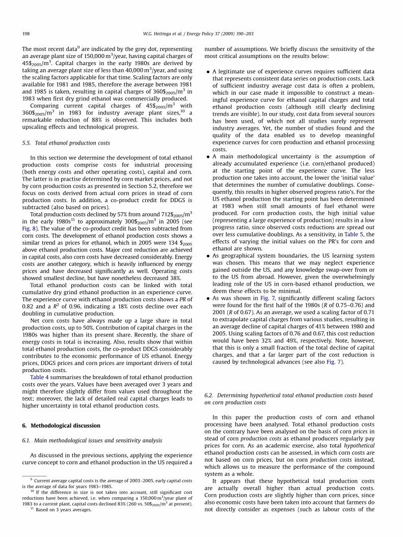
Fig. 2 shows the decline in US corn production costs over theperiod 1975–2005. Production costs of corn declined by 62%, from

ARTICLE IN PRESS
0
50
100
150
200
250
300
350
1975
Cor
n pr
oduc
tion
cos
ts [
$(20
05)/
tonn
e]
General farm overheadCustom operationsRepairsLabour (hired and unpaid labour)ChemicalsSeedFuel, lube and electrictyFertilizer (incl soil conditioners: lime and gypsum)Taxes, insurance and land rentCapital recovery incl interest
1980 1985 1990 1995 2000 2005
Fig. 2. Breakdown of corn production costs 1975–2005. (Data source: USDA/ERS, 2007).
Cumulative corn production [109 T]
1052.5
Cor
n pr
oduc
tion
cost
s [$
2005
/tonn
e]
100
200
400
Corn production costs per tonnePR = 0.55 ±± 0.02 (R2 = 0.87)
1975
2005
Fig. 3. Experience curve on corn production costs.
W.G. Hettinga et al. / Energy Policy 37 (2009) 190–203 195
260$2005/tonne in 1975 to 100$2005/tonne in 2005.6 If the effect ofincreasing yields is excluded by analysing costs per hectare, stillcosts have declined by 35%. High cost reductions are observed inthe early 1980s. After 1985 costs per hectare remained fairlyconstant, but ever increasing yields drove the production costsfurther down. Due to crop losses in 1980, 1983, 1988, 1993 and1995, costs per tonne were considerably higher (for underlyingcauses, see: Hettinga, 2007).
Costs for ‘taxes, insurance and land rent’, ‘capital recovery’ and‘fertilizer’ are the most important categories showing both highestshares in total production costs, and largest contributions tooverall cost decline. Also ‘farm overhead’ costs have declinedremarkably. Rising energy prices over the last 3 years resulted inhigher costs for fuels, electricity and fertilizer. But increasing yieldoutbalanced the higher costs for fertilizer, resulting in a decline offertilizer costs per tonne. Costs for fuels and electricity havenonetheless increased per tonne. Fig. 2 shows the breakdown ofcorn production costs.
Fig. 3 shows the relationship between corn production andproduction costs by means of an experience curve. Corn produc-tion costs have been reduced by 62% over 1.85 doublings incumulative production, resulting in a PR of 0.5570.02(R2¼ 0.87).7 This states that corn production costs per tonne
declined 45% over each doubling in cumulative production. Byexcluding major weather influences (as identified in Hettinga,2007) the PR is unchanged, but the fit improves (R2
¼ 0.91), whichindicates of good representation of reality.
The sharp decline of production costs in 1986 is mostlycaused by decreasing capital and land costs. Likely, the observedshakeout among small-scale farmers led to a higher availability ofcapital and land, and thus to lower prices for these categories. Ingeneral, much of the cost decline can be attributed to indirect‘overhead’ categories, direct input costs have decreased less. Thefact that several inputs categories have a direct positive effect onachieving higher yields strengthens this observation. Indirectcosts are more dependent on farm size and subject to economiesof scale.
6 Three year averages have been used, so 1975–1977 and 2003–2005 to
exclude annual fluctuations.7 R2 gives an estimate in the amount of variation explained by the model and
provides information about the goodness-of-fit of a model. R2’s are commonly
quoted in papers on experience curves.
5.3. Development of ethanol processing costs
Fig. 4 shows the development of industrial processing costsover time and presents a breakdown into several categories.Industrial processing costs mainly include costs for energy,enzymes, labour, maintenance and chemicals. Costs for corn andcapital are not assessed in this section. Processing costs of ethanoldeclined between 40% and 50%, from around 240$2005/m3 in 1983to below 130$2005/m3 in 2005.8
The largest cost decline occurred in the early 1990s, when costsdropped from levels above 200$2005/m3 to below 150$2005/m3.The slight increase towards 2005 is mainly caused by increasingenergy prices. The available studies also show a larger decrease atfirst (1987–1998), which flattens out towards the end(1998–2002).
Energy costs (fossil fuels and electricity) represent the largestpart (�40% in 3 surveyed years). Important other cost categoriesare labour, enzymes and chemicals (mostly yeast and chemicalsused for boiler and process water treatment). Insufficient datalimits a detailed quantitative analysis of the various categories to
8 The average processing costs for 1983–1984 and 2004–2005 have been
averaged.

ARTICLE IN PRESS
0
50
100
150
200
250
300
1981
1982
(LeB
lanc &
Pra
to, 1
982)
198
3
(Keim
, 198
3) 1
984
(Halb
ach
& F
ruin
, 198
6) 1
985
(Swan
k et
al., 1
987)
198
6
Kane &
Reil
ly, 1
989)
198
7
(Keim
, 198
9) 1
988
(Woo
d, 1
993)
199
2
(Katz
en et
al.,
1994
) 199
4(S
hapo
uri e
tal .,
200
2b) 1
998
(McA
loon
et al
., 20
00) 1
999
(BBI,
2000
) 200
0
(Whi
ms,
2002
) 200
1
(Sha
pour
i & G
allag
her,
2005
) 200
2
(Tiff
any
& E
idm
an, 2
003)
200
3
(R.W
.Bec
k,20
04) 2
004
(ERRC, 2
007)
200
5
Indu
stri
al p
roce
ssin
g co
sts
[$(2
005)
/m3 ]
FuelsElectricityTotal energy costsOtherGeneral administrationTax and insuranceChemicals (incl. yeast and water)DenaturantMaintenanceEnzymesLabour
Fig. 4. Breakdown of ethanol processing costs between 1980 and 2005. Engineering studies of 1981 and 1982 are assumed to represent actual costs for 1983 and 1984. Note
that different studies use different cost structures (LeBlanc and Prato, 1983; Keim, 1983; Halbach and Fruin, 1986; Swank et al., 1987; Kane and Reilly, 1989; Keim, 1989;
Wood, 1993; Katzen et al., 1994; Shapouri et al., 2002b; McAloon et al., 2000; BBI, 2000; Whims, 2002; Shapouri and Gallagher, 2005; Tiffany and Eidman, 2003; Beck,
2004; ERRC, 2007).
Table 3The decline in ethanol processing costs and its main contributors
Early 1980s 2005 Reduction (%)
$2005/m3 Share in total costs (%) $2005/m3 Share in total costs (%)
Energy costs 140 58 70 54 50
Labour costs 55 23 16 12 70
Enzyme costs 40 17 10 8 75
Total 240 98 130 74 40–50
W.G. Hettinga et al. / Energy Policy 37 (2009) 190–203196
development in costs for energy, labour and enzymes, but mostimportant categories are highlighted in Table 3. Other qualitativecost-reducing developments and technological changes have beendescribed in Section 5.1.
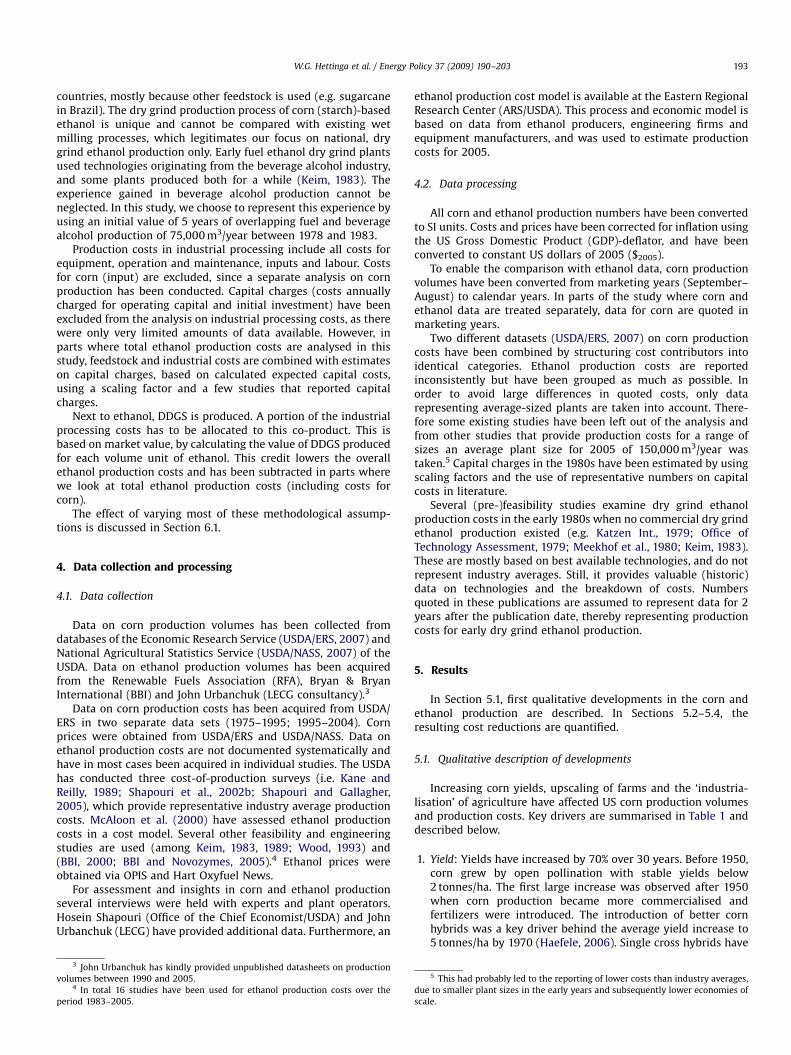
Energy costs are the largest contributor of processing costs.The cost reduction is caused by the decrease in energy consump-tion as can be seen in Fig. 5. Increasing prices for energy haveincreased the pressure on producers to implement energy-efficient production technologies. Furthermore, debates on theenergy balance of US ethanol have stimulated optimisation onenergy use. Average dry grind plants used 22 GJ/m3 in the early1980s that has been reduced to below 10 GJ/m3 for presentaverage dry grind plants. In Fig. 5, various studies on energyconsumption in ethanol production over the years is plotted. Inthis graph only industrial energy use is displayed. Large energyefficiency gains are visible in the late 1980s. This is mostly causedby the replacement of dehydration technologies, and otherdevelopments described in Section 5.2. Hettinga (2007) assessedenergy consumption as a performance indicator for technologicallearning in experience curves.
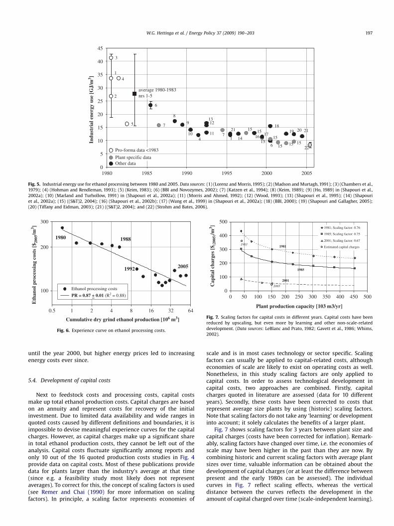
By plotting cumulative dry grind ethanol production againstindustrial processing costs, an experience curve is constructed(see Fig. 6). Cumulative dry grind ethanol production doubled 7.2times since 1983 (see gridlines in graph). Over the sametimeframe costs have been reduced by 45% on average. Theprogress ratio of this curve is given 0.8770.01 with a reliable fit ofR2¼ 0.88. This indicates that ethanol processing costs decline 13%
per doubling in cumulative production.The large decline in ethanol processing costs between 1988
and 1992 parallels with the shift in the industry towardsoptimised ethanol production technologies that were designedfor fuel ethanol production only. Beverage-based technologies wasphased out in the industry, since new dry grind plants were beingbuilt rapidly. Most of the described technological developments inSection 5.1 occurred at the end of the 1980s, such as theintroduction of molecular sieves, distributed control systemsand SSF technologies. Industry average costs from the 1990sonwards settled at about 125$2005/m3. Improved efficiencies andoperation lowered operating expenses, even though since 2003varying numbers are quoted. Costs for energy have decreased
ARTICLE IN PRESS
Cumulative dry grind ethanol production [106 m3]
0.5 1 2 4 8 16 32 64
Eth
anol
pro
cess
ing
cost
s [$
2005
/m3 ]
100
200
300
Ethanol processing costs
PR = 0.87 + 0.01 (R2 = 0.88)
2005
1980 1988
1992
Fig. 6. Experience curve on ethanol processing costs.
1981
1985
2001
2005
1983
0
100
200
300
400
500
0
Plant production capacity [103 m3/yr]
Cap
ital
cha
rges
[$ (
2005
)/m3 ] 1981; Scaling factor: 0.76
1985; Scaling factor: 0.75
2001; Scaling factor: 0.67
Estimated capital charges
50 100 150 200 250 300 350 400 450 500
Fig. 7. Scaling factors for capital costs in different years. Capital costs have been
reduced by upscaling, but even more by learning and other non-scale-related
development. (Data sources: LeBlanc and Prato, 1982; Gavett et al., 1986; Whims,
2002).
3
5
6
7 18
Plant specific data
Pro-forma data <1983
Other data
1
1
2
4
4
6
7
8
9
10 11
1213
14
1515
1515
15 15 1516 17
19
22
20
average 1980-1983nrs 1-5
2121
0
5
10
15
20
25
30
35
40
45
1980
Indu
stri
al e
nerg
y us
e [G
J/m
3 ]
1985 1990 1995 2000 2005
Fig. 5. Industrial energy use for ethanol processing between 1980 and 2005. Data sources: (1) (Lorenz and Morris, 1995); (2) (Madson and Murtagh, 1991); (3) (Chambers et al.,
1979); (4) (Hohman and Rendleman, 1993); (5) (Keim, 1983); (6) (BBI and Novozymes, 2002); (7) (Katzen et al., 1994); (8) (Keim, 1989); (9) (Ho, 1989) in (Shapouri et al.,
2002a); (10) (Marland and Turhollow, 1991) in (Shapouri et al., 2002a); (11) (Morris and Ahmed, 1992); (12) (Wood, 1993); (13) (Shapouri et al., 1995); (14) (Shapouri
et al., 2002a); (15) ((S&T)2, 2004); (16) (Shapouri et al., 2002b); (17) (Wang et al., 1999) in (Shapouri et al., 2002a); (18) (BBI, 2000); (19) (Shapouri and Gallagher, 2005);
(20) (Tiffany and Eidman, 2003); (21) ((S&T)2, 2004); and (22) (Strohm and Bates, 2006).
W.G. Hettinga et al. / Energy Policy 37 (2009) 190–203 197
until the year 2000, but higher energy prices led to increasingenergy costs ever since.
5.4. Development of capital costs
Next to feedstock costs and processing costs, capital costsmake up total ethanol production costs. Capital charges are basedon an annuity and represent costs for recovery of the initialinvestment. Due to limited data availability and wide ranges inquoted costs caused by different definitions and boundaries, it isimpossible to devise meaningful experience curves for the capitalcharges. However, as capital charges make up a significant sharein total ethanol production costs, they cannot be left out of theanalysis. Capital costs fluctuate significantly among reports andonly 10 out of the 16 quoted production costs studies in Fig. 4provide data on capital costs. Most of these publications providedata for plants larger than the industry’s average at that time(since e.g. a feasibility study most likely does not representaverages). To correct for this, the concept of scaling factors is used(see Remer and Chai (1990) for more information on scalingfactors). In principle, a scaling factor represents economies of
scale and is in most cases technology or sector specific. Scalingfactors can usually be applied to capital-related costs, althougheconomies of scale are likely to exist on operating costs as well.Nonetheless, in this study scaling factors are only applied tocapital costs. In order to assess technological development incapital costs, two approaches are combined. Firstly, capitalcharges quoted in literature are assessed (data for 10 differentyears). Secondly, these costs have been corrected to costs thatrepresent average size plants by using (historic) scaling factors.Note that scaling factors do not take any ‘learning’ or developmentinto account; it solely calculates the benefits of a larger plant.
Fig. 7 shows scaling factors for 3 years between plant size andcapital charges (costs have been corrected for inflation). Remark-ably, scaling factors have changed over time, i.e. the economies ofscale may have been higher in the past than they are now. Bycombining historic and current scaling factors with average plantsizes over time, valuable information can be obtained about thedevelopment of capital charges (or at least the difference betweenpresent and the early 1980s can be assessed). The individualcurves in Fig. 7 reflect scaling effects, whereas the verticaldistance between the curves reflects the development in theamount of capital charged over time (scale-independent learning).
ARTICLE IN PRESS
W.G. Hettinga et al. / Energy Policy 37 (2009) 190–203198
The most recent data9 are indicated by the grey dot, representingan average plant size of 150,000 m3/year, having capital charges of45$2005/m3. Capital charges in the early 1980s are derived bytaking an average plant size of less than 40,000 m3/year, and usingthe scaling factors applicable for that time. Scaling factors are onlyavailable for 1981 and 1985, therefore the average between 1981and 1985 is taken, resulting in capital charges of 360$2005/m3 in1983 when first dry grind ethanol was commercially produced.
Comparing current capital charges of 45$2005/m3 with360$2005/m3 in 1983 for industry average plant sizes,10 aremarkable reduction of 88% is observed. This includes bothupscaling effects and technological progress.
5.5. Total ethanol production costs
In this section we determine the development of total ethanolproduction costs comprise costs for industrial processing(both energy costs and other operating costs), capital and corn.The latter is in practise determined by corn market prices, and notby corn production costs as presented in Section 5.2, therefore wefocus on costs derived from actual corn prices in stead of cornproduction costs. In addition, a co-product credit for DDGS issubtracted (also based on prices).
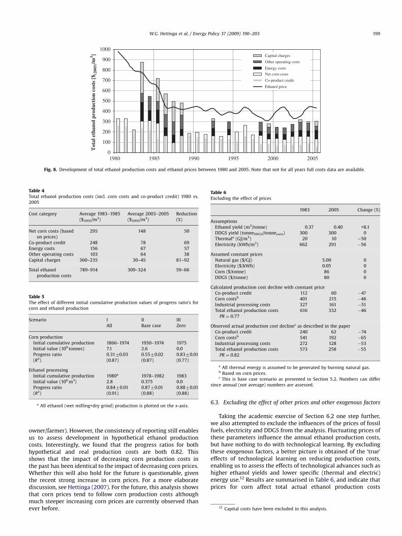
Total production costs declined by 57% from around 712$2005/m3
in the early 1980s11 to approximately 300$2005/m3 in 2005 (seeFig. 8). The value of the co-product credit has been subtracted fromcorn costs. The development of ethanol production costs shows asimilar trend as prices for ethanol, which in 2005 were 134 $2005
above ethanol production costs. Major cost reduction are achievedin capital costs, also corn costs have decreased considerably. Energycosts are another category, which is heavily influenced by energyprices and have decreased significantly as well. Operating costsshowed smallest decline, but have nonetheless decreased 38%.
Total ethanol production costs can be linked with totalcumulative dry grind ethanol production in an experience curve.The experience curve with ethanol production costs shows a PR of0.82 and a R2 of 0.96, indicating a 18% costs decline over eachdoubling in cumulative production.
Net corn costs have always made up a large share in totalproduction costs, up to 50%. Contribution of capital charges in the1980s was higher than its present share. Recently, the share ofenergy costs in total is increasing. Also, results show that withintotal ethanol production costs, the co-product DDGS considerablycontributes to the economic performance of US ethanol. Energyprices, DDGS prices and corn prices are important drivers of totalproduction costs.
Table 4 summarises the breakdown of total ethanol productioncosts over the years. Values have been averaged over 3 years andmight therefore slightly differ from values used throughout thetext; moreover, the lack of detailed real capital charges leads tohigher uncertainty in total ethanol production costs.
6. Methodological discussion
6.1. Main methodological issues and sensitivity analysis
As discussed in the previous sections, applying the experiencecurve concept to corn and ethanol production in the US required a
9 Current average capital costs is the average of 2003–2005, early capital costs
is the average of data for years 1983–1985.10 If the difference in size is not taken into account, still significant cost
reductions have been achieved, i.e. when comparing a 150,000 m3/year plant of
1983 to a current plant, capital costs declined 83% (260 vs. 50$2005/m3 at present).11 Based on 3 years averages.
number of assumptions. We briefly discuss the sensitivity of themost critical assumptions on the results below:
�
A legitimate use of experience curves requires sufficient datathat represents consistent data series on production costs. Lackof sufficient industry average cost data is often a problem,which in our case made it impossible to construct a mean-ingful experience curve for ethanol capital charges and totalethanol production costs (although still clearly decliningtrends are visible). In our study, cost data from several sourceshas been used, of which not all studies surely representindustry averages. Yet, the number of studies found and thequality of the data enabled us to develop meaningfulexperience curves for corn production and ethanol processingcosts. � A main methodological uncertainty is the assumption ofalready accumulated experience (i.e. corn/ethanol produced)at the starting point of the experience curve. The lessproduction one takes into account, the lower the ‘initial value’that determines the number of cumulative doublings. Conse-quently, this results in higher observed progress ratio’s. For theUS ethanol production the starting point has been determinedat 1983 when still small amounts of fuel ethanol wereproduced. For corn production costs, the high initial value(representing a large experience of production) results in a lowprogress ratio, since observed costs reductions are spread outover less cumulative doublings. As a sensitivity, in Table 5, theeffects of varying the initial values on the PR’s for corn andethanol are shown.
� As geographical system boundaries, the US learning systemwas chosen. This means that we may neglect experiencegained outside the US, and any knowledge swap-over from orto the US from abroad. However, given the overwhelminglyleading role of the US in corn-based ethanol production, wedeem these effects to be minimal.
� As was shown in Fig. 7, significantly different scaling factorswere found for the first half of the 1980s (R of 0.75–0.76) and2001 (R of 0.67). As an average, we used a scaling factor of 0.71to extrapolate capital charges from various studies, resulting inan average decline of capital charges of 41% between 1980 and2005. Using scaling factors of 0.76 and 0.67, this cost reductionwould have been 32% and 49%, respectively. Note, however,that this is only a small fraction of the total decline of capitalcharges, and that a far larger part of the cost reduction iscaused by technological advances (see also Fig. 7).
6.2. Determining hypothetical total ethanol production costs based
on corn production costs
In this paper the production costs of corn and ethanolprocessing have been analysed. Total ethanol production costson the contrary have been analysed on the basis of corn prices instead of corn production costs as ethanol producers regularly payprices for corn. As an academic exercise, also total hypothetical
ethanol production costs can be assessed, in which corn costs arenot based on corn prices, but on corn production costs instead,which allows us to measure the performance of the compoundsystem as a whole.
It appears that these hypothetical total production costsare actually overall higher than actual production costs.Corn production costs are slightly higher than corn prices, sincealso economic costs have been taken into account that farmers donot directly consider as expenses (such as labour costs of the
ARTICLE IN PRESS
0
100
200
300
400
500
600
700
800
900
1000
1980
Tot
al e
than
ol p
rodu
ctio
n co
sts
[$(2
005)
/m3 ] Capital charges
Other operating costs
Energy costs
Net corn costs
Co-product credit
Ethanol price
1985 1990 1995 2000 2005
Fig. 8. Development of total ethanol production costs and ethanol prices between 1980 and 2005. Note that not for all years full costs data are available.
Table 4Total ethanol production costs (incl. corn costs and co-product credit) 1980 vs.
2005
Cost category Average 1983–1985
($2005/m3)
Average 2003–2005
($2005/m3)
Reduction
(%)
Net corn costs (based
on prices)
295 148 50
Co-product credit 248 78 69
Energy costs 156 67 57
Other operating costs 103 64 38
Capital charges 360–235 30–45 81–92
Total ethanol
production costs
789–914 309–324 59–66
Table 5The effect of different initial cumulative production values of progress ratio’s for
corn and ethanol production
Scenario I II III
All Base case Zero
Corn production
Initial cumulative production 1866–1974 1950–1974 1975
Initial value (109 tonnes) 7.1 2.6 0.0
Progress ratio 0.3170.03 0.5570.02 0.8370.01
(R2) (0.87) (0.87) (0.77)
Ethanol processing
Initial cumulative production 1980a 1978–1982 1983
Initial value (106 m3) 2.8 0.375 0.0
Progress ratio 0.8470.01 0.8770.01 0.8870.01
(R2) (0.91) (0.88) (0.88)
a All ethanol (wet milling+dry grind) production is plotted on the x-axis.
Table 6Excluding the effect of prices
1983 2005 Change (%)
Assumptions
Ethanol yield (m3/tonne) 0.37 0.40 +8.1
DDGS yield (tonneDDGS/tonnecorn) 300 300 0
Thermala (GJ/m3) 20 10 �50
Electricity (kWh/m3) 662 291 �56
Assumed constant prices
Natural gas ($/GJ) 5.00 0
Electricity ($/kWh) 0.05 0
Corn ($/tonne) 86 0
DDGS ($/tonne) 80 0
Calculated production cost decline with constant price
Co-product credit 112 60 �47
Corn costsb 401 215 �46
Industrial processing costs 327 161 �51
Total ethanol production costs 616 332 �46
PR ¼ 0.77
Observed actual production cost declinec as described in the paper
Co-product credit 240 62 �74
Corn costsb 541 192 �65
Industrial processing costs 272 128 �53
Total ethanol production costs 573 258 �55
PR ¼ 0.82
a All thermal energy is assumed to be generated by burning natural gas.b Based on corn prices.c This is base case scenario as presented in Section 5.2. Numbers can differ
since annual (not average) numbers are assessed.
12 Capital costs have been excluded in this analysis.
W.G. Hettinga et al. / Energy Policy 37 (2009) 190–203 199
owner/farmer). However, the consistency of reporting still enablesus to assess development in hypothetical ethanol productioncosts. Interestingly, we found that the progress ratios for bothhypothetical and real production costs are both 0.82. Thisshows that the impact of decreasing corn production costs inthe past has been identical to the impact of decreasing corn prices.Whether this will also hold for the future is questionable, giventhe recent strong increase in corn prices. For a more elaboratediscussion, see Hettinga (2007). For the future, this analysis showsthat corn prices tend to follow corn production costs althoughmuch steeper increasing corn prices are currently observed thanever before.
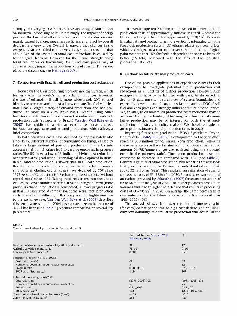
6.3. Excluding the effect of other prices and other exogenous factors
Taking the academic exercise of Section 6.2 one step further,we also attempted to exclude the influences of the prices of fossilfuels, electricity and DDGS from the analysis. Fluctuating prices ofthese parameters influence the annual ethanol production costs,but have nothing to do with technological learning. By excludingthese exogenous factors, a better picture is obtained of the ‘true’effects of technological learning on reducing production costs,enabling us to assess the effects of technological advances such ashigher ethanol yields and lower specific (thermal and electric)energy use.12 Results are summarised in Table 6, and indicate thatprices for corn affect total actual ethanol production costs
ARTICLE IN PRESS
W.G. Hettinga et al. / Energy Policy 37 (2009) 190–203200
strongly, but varying DDGS prices have also a significant impacton industrial processing costs. Interestingly, the impact of energyprices is the lowest of all variable categories. Cost reductions aremainly caused by increasing energy efficiencies and not by overalldecreasing energy prices Overall, it appears that changes in theexogenous factors added to the overall costs reductions, but thatabout 84% of the overall ethanol cost reductions is caused bytechnological learning. However, for the future, strongly risingfossil fuel prices or fluctuating DGGS and corn prices may ofcourse strongly impact the production costs of ethanol. For a moreelaborate discussion, see Hettinga (2007).
7. Comparison with Brazilian ethanol production cost reductions
Nowadays the US is producing more ethanol than Brazil, whichformerly was the world’s largest ethanol producer. However,the use of ethanol in Brazil is more widespread: 20% ethanolblends are common and almost all new cars are flex fuel vehicles.Brazil has a longer history of ethanol production and has pro-duced far more on a cumulative basis. Despite using otherfeedstock, similarities can be drawn in the reduction of feedstockproduction costs (sugarcane for Brazil). Van den Wall Bake et al.(2008) has published a similar experience curve analysisfor Brazilian sugarcane and ethanol production, which allows abrief comparison.
In both countries costs have declined by approximately 60%since 1975. Different numbers of cumulative doublings, caused bytaking a large amount of previous production in the US intoaccount (high initial value) lead to varying outcomes in progressratios. The US shows a lower PR, indicating higher cost reductionsover cumulative production. Technological development in Brazi-lian sugarcane production is slower than in US corn production.Brazilian ethanol production started earlier and ethanol proces-sing costs (including capital costs) have declined by 70% since1975 versus 49% reduction is US ethanol processing costs (withoutcapital costs) since 1983. Taking these reductions into account aswell as the lower number of cumulative doublings in Brazil (moreprevious ethanol production is considered), a lower progress ratioin Brazil is calculated. A comparison of the actual total productioncosts of ethanol is difficult, as this comparison is highly sensitiveto the exchange rate. Van den Wall Bake et al. (2008) describesthis sensitiveness and for 2004 costs an average exchange rate of3.6 R$ has been used Table 7 presents a comparison on several keyparameters.
Table 7Comparison of ethanol production in Brazil and the US
Total cumulative ethanol produced by 2005 (million m3)
Agricultural yield (tonnecane/ha)
Ethanol yield (m3/tonnecane)
Feedstock production (1975–2005)
Cost reduction (%)
Number of doublings in cumulative production
Progress ratio
2005 costs ($/tonnecane)
Industrial processing (start-2005)
Cost reduction
Number of doublings in cumulative production
Progress ratio
2005 costs ($/m3)
Current total ethanol production costs ($/m3)
Current ethanol price ($/m3)
The overall experience of production has led to current ethanolproduction costs of approximately 188$/m3 in Brazil, whereas theUS is producing ethanol for approximately 310$/m3. WhereasBrazilian ethanol production is more vertically integrated with thefeedstock production system, US ethanol plants pay corn prices,which are subject to a current increases. From a methodologicalpoint we note that PR’s for feedstock production seem to be muchbetter (55–68%) compared with the PR’s of the industrialprocessing (81–87%).
8. Outlook on future ethanol production costs
One of the possible applications of experience curves is theirextrapolation to investigate potential future production costreductions as a function of further production. However, suchextrapolations have to be handled with care. As discussed, inSection 6, data uncertainties, choices of system boundaries andespecially development of exogenous factors such as DDG, fossilfuel and corn prices can strongly influence future ethanol prices.Yet, an analysis on how much production costs reductions may beachieved through technological learning as a function of cumu-lative production may be of interest for both the ethanol-producing industry and policy makers. We therefore made anattempt to estimate ethanol production costs in 2020.
Regarding future corn production, USDA’s Agricultural Projec-tion to 2016 (USDA/OCE, 2007) is extrapolated to the year 2020,reaching 370 million tonnes annual corn production. Followingthe experience curve the estimated corn production costs in 2020amount 74–76$/tonne (ranges are achieved using the standarderror in the progress ratio). Thus, corn production costs areestimated to decrease 30% compared with 2005 (see Table 8).Concerning future ethanol production, two scenarios are assessed:firstly, extrapolation of the Renewable Fuels Standard until 2020(up to 52 million m3/year). This results in an estimation of ethanolprocessing costs of 69–77$/m3 in 2020. Secondly, extrapolation ofan outlook provided by Urbanchuk (2007) forecasts production ofup to 68 million m3/year in 2020. The higher predicted productionvolumes will lead to higher cost decline that results in processingcosts of 60–70$/m3 in 2020. On average the same percentage ofcost reduction for the future is expected as has occurred over1983–2005 (46%).
This analysis shows that lower (i.e. better) progress ratios(for corn) do not per se lead to high cost decline, as until 2020,only few doublings of cumulative production will occur. On the
Brazil (data from Van den Wall
Bake et al., 2008)
US
300 125
75–82 9–10
0.082 0.4
60 63
3 1.9
0.6870.03 0.5570.02
14.9 107
(1975–2005) 70% (1983–2005) 49%
5 7.2
0.8170.02 0.8770.01
103 128 (+50$ capital)
�188 �310
365 430

ARTICLE IN PRESS
Table 8Corn and ethanol production costs in 2020, calculated by extrapolating the experience curve (RFA, 2008; Urbanchuk, 2007; USDA/OCE, 2007)
Corn production USDA agricultural projection (extrapolated)
2005 production costs 107$2005/tonne
Predicted cumulative production in 2020 (1975–2020) 14�109 tonne
2020 predicted production costs 74–76$2005/tonne
Ethanol processing I. RFS extrapolated II. Urbanchuk outlook
2005 production costs (minus corn and capital costs) ($2005/m3) 128 128
Predicted cumulative production in 2020 (1983–2020) (�106 m3) 560 767
2020 predicted production costs ($2005/m3) 69–77 60–70
W.G. Hettinga et al. / Energy Policy 37 (2009) 190–203 201
other hand, a high (i.e. less benign) progress ratio for ethanolprocessing nevertheless results in relatively high cost reductionbecause of large predicted future ethanol production volumes,leading to several further doublings of cumulative production.
Ideally, to support these findings, they should be comparedwith expectations from bottom-up engineering studies for futurecost reduction potentials. Unfortunately, while several studiesexist that examine the impact of new production processtechnologies on production costs, and these clearly show furthertechnical improvement potential, we did not find an integratedanalysis that combines these various studies. Rendleman andShapouri (2007) expect savings in the future to be smaller thanthose of the last 10–15 years, since ethanol production isbecoming a mature industry, thus representing a more conserva-tive estimate than our analysis. A brief analysis of a paper that waspublished by Argonne National Laboratory (Wu, 2008) shortlyafter the final findings of this paper shows that significantefficiency gains have been observed in the ethanol industry since2002. Amongst others, ethanol yield increased by 6%, lessproducers dry the DDG, which saves energy. The industry’saverage energy use in 2007 amounted 7.8 GJ/m3, which issupported by our data and extrapolation. This strengthens ouranalysis on energy and its decline over time or accumulatedproduction. We recommend further research on a better compar-ison of bottom-up engineering and top-down experience curveanalysis results in order to identify areas of possible furtherimprovement.
We emphasise again, that the cost reduction outlook is solelybased on further technological progress. Although this studyshows that ethanol processing costs (including energy costs,excluding corn and capital costs) have decreased in the past,especially corn price developments are highly uncertain. Currentspeculation on ethanol demand leads to extraordinary high cornspot prices (up to 160$/tonne). While these have so far littleinfluenced long-term corn supply contracts of ethanol plants, alsoin long-term projections (USDA/OCE, 2007) an increase in cornprices is expected.
9. Summary and conclusions
The objective of this study was to assess technological learningby quantifying reductions in production costs and energy use inUS ethanol production. This technological learning can beidentified in two separate systems: corn production and ethanolprocessing.
Corn production costs declined by 62% over the period1975–2005. Main drivers behind cost reductions are higher cornyields and the upscaling of farms. Ethanol processing costs(without corn and capital costs) declined by 45% over the period1983–2005. Costs for energy, labour and enzymes contribute most
to overall cost decline. Key drivers behind these reductions arehigher ethanol yields, the introduction of fuel ethanol specific andautomated technologies that require less energy and labour.Recent higher energy prices have partly outbalanced reductions inother operating costs. Overall, corn prices determine feedstockcosts for the ethanol producer, which have shown decreases aswell (caused by more than just technological learning in cornproduction). Total ethanol production costs, which include capitaland net corn costs, have declined by 57% since 1983. Costsreductions have been achieved throughout the entire productionchain, i.e. net corn costs, industrial processing costs and capitalcosts have all contributed to overall cost decline.
The analysis has shown that corn production and ethanolprocessing costs have decreased with cumulative production andthat the experience curve concept can be used to describe thistrend reliably. The calculations on the experience curve present aprogress ratio of 0.5570.02 for corn production costs over theperiod 1975–2005. A progress ratio of 0.8770.01 is calculated forindustrial processing costs (without costs for corn and capital)since 1983. A comparison with Brazilian sugarcane and ethanolproduction reveal similar PRs for feedstock and industrialprocessing cost reductions.
Experience curves can also be used as a tool to assess futurecost decline by taking projected production and detailed costbreakdowns into account. Extrapolating these experience curvesto 2020, corn production costs are estimated to amount 75$ pertonne in 2020. Ethanol processing costs (without costs for cornand capital) are expected to come with the range of $60–$77 perm3 in 2020. These are both significant further reductions, mostlydriven by the large expected volumes of future (corn-derived)ethanol production. On the other hand, prices for corn and energyare expected to rise in the future, which ultimately determineethanol production costs for the producer of which prices paid forcorn will be most decisive. Also, ethanol prices closely correlatewith gasoline prices, leading to expected higher ethanol prices inthe future as well.
We conclude that experience curves are an adequate tool toanalyse past technological learning and resulting cost reductionsfor US corn-based ethanol production, and, keeping all limitationsof the analysis in mind, also show a significant cost reductionpotential for the future.
Next to use within the ethanol-producing industry itself, theinsights gained from this analysis may also be of relevance forpolicy makers. They show that despite being a ‘first-generation’technology, significant further cost reductions may occur due totechnological learning in the coming years. This indicates thatfuture second-generation fuels (e.g. cellulose-derived ethanol)may have to receive extra support not only to compete withgasoline, but also with corn-derived ethanol. Furthermore, theexpected cost reductions could be useful to review US policies one.g. the future level of corn subsidy programs, and the blender tax
ARTICLE IN PRESS
W.G. Hettinga et al. / Energy Policy 37 (2009) 190–203202
credit, and the necessity of ethanol import tariffs (for Brazilianethanol). Discussing this in detail would extend the scope of thispaper, we refer to Hettinga (2007) for a more detailed treatmentof the topic.
Finally, the empirically found PR’s for corn and ethanolproduction may also be of use for science, e.g. for use inenergy models. Regarding recommendations or further research,we would like to emphasise that the developments in theenergy efficiency of corn-based ethanol production deservesfurther attention. As shown in Fig. 5, energy inputs have decreasedsignificantly since 1980, though especially within the firsthalf of the 1980s. Future improvements in energy efficiency maylead to lower costs, but also to lower GHG emissions. Whetherthese efficiency improvements actually also follow an experiencecurve pattern (e.g. similar to ammonia production as found byRamirez and Worrell, 2006) is a question worthwhile exploringfurther.
Acknowledgements
The authors would like to thank the following persons: HoseinShapouri (Office of the Chief Economist, USDA), JohnUrbanchuk (LECG consultancy), Phil Madson (Katzen Interna-tional), Larry Schafer (Renewable Fuels Association), Kelly Davis(Chippewa Valley Ethanol Company), Bruce Strohm & David Bates(Genencor), Doug Haefele (Pioneer), Paul Gallagher (Iowa StateUniversity), Philip Shane (Illinois Corn Growers Association),Charles Abbas & Kyle Beery (Archer Daniels Midland), and MaxStarbuck & Geoff Cooper (National Corn Growers Association) forsharing their valuable insights and data. The first author wouldlike to express his gratitude to the Eastern Regional ResearchCenter (ARS/USDA) for financial and logistic support.
References
BBI, 2000. Iowa Ethanol Plant Pre-Feasibility Study. Bryan & Bryan InternationalInc. (BBI), Cotopaxi, CO, USA.
BBI and Novozymes, 2002. Fuel Ethanol Production: Technological and Environ-mental Improvements. Novozymes and BBI, Colorado, USA.
BBI and Novozymes, 2005. Fuel Ethanol: A Technological Evolution. Novozymesand BBI, Colorado, USA.
Beck, R.W., 2004. Corn to Ethanol Bulletins. Renewable Energy Bulletin.Chambers, R.S., Herendeen, R.A., Joyce, J.J., Penner, P.S., 1979. Gasohol: does it or
doesn’t it produce positive net energy. Science 206, 189–795.Coltrain, D., Dean, E., Barton, D., 2004. Risk Factors in Ethanol Production.
Department of Agricultural Economics, Kansas State University.EIA, 2007. Official Energy Statistics from the US Government. Energy Information
Administration, United States Department of Energy Available at /http://eia.doe.govS Visited between August 2006–May 2007.
ERRC, 2007. 40 Million Gallon Dry Grind Ethanol Production Process and CostModel. Available from Andrew McAloon at the Eastern Regional ResearchCenter, ARS, USDA.
Foreman, L., 2001. Characteristics and Production Costs of US Corn Farms. SBN-974.USDA, Economic Research Service.
Foreman, L., 2006. Characteristics and Production Costs of US Corn Farms, 2001.Economic Research Service, Economic Information Bulletin no. 7, Washington,DC.
Gavett, E.E., Grinnell, G.E., Smith, N.L., 1986. Fuel Ethanol and Agriculture: AnEconomic Assessment. Office of Energy, USDA, AER-562, Washington, DC.
Grubler, A., Nakicenovic, N., Victor, D.G., 1999. Dynamics of Energy Technologiesand Global Change. Energy Policy 27, 247–280.
Haefele, D., 2006. Pioneer. Personal Communication. Several email communica-tions, August–December 2006.
Halbach, D.W., Fruin, J.E., 1986. The Economics of ethanol production and itsimpact on the Minnesota farm community. Staff Paper P0090-1334 Universityof Minnesota, Department of Agricultural and Applied Economics.
Hansen, R., 2006. Ethanol Profile. Agricultural Marketing Resource Center (AgMRC),Iowa State University.
Hettinga, W.G., 2007. Technological learning in US ethanol production. Includingappendices, Master Thesis, Copernicus Institute, Utrecht University, TheNetherlands, available at website.
Ho, S.P., 1989. Global warming impact of ethanol versus gasoline. Presented at 1989National Conference. Clean Air Issues and America’s Motor Fuel Business,Washington, DC.
Hohman, N., Rendleman, C.M., 1993. Emerging Technologies in Ethanol Production.AIB-663, USDA, Economic Research Service.
IEA/OECD, 2000. Experience Curves for Energy Technology Policy. Paris, France.Junginger, M., 2005. Learning in Renewable Energy Technology Development. Ph.D.
Thesis, Utrecht University, The Netherlands.Kane, S.M., Reilly, J.M., 1989. Economics of Ethanol Production in the United States.
AER-607, USDA, Economic Research Service.Katzen, R., Madson, P.W., Shroff, B.S., 1994. Ethanol from corn: state-of-the-art
technology and economics. Prepared for Presentation at National CornGrowers Association Con Utilization Conference V, Unpublished, June 1994.
Katzen Int., 1979. Grain Motor Fuel Ethanol: Technical and Economic AssessmentStudy. US Department of Energy, Cincinnati, OH, USA.
Keim, C.R., 1983. Technology and economics of fermentation alcohol—an update.Enzyme and Microbiology Technology 5 (March), 103–114.
Keim, C.R., 1989. Fuel ethanol. In: U.S. Gasoline Outlook 1989–2004: ChangingDemands, Values and Regulations. Information Resources, Washington, DC.
Leath, M.N., Meyer, L.H., Hill, L.D., 1982. U.S. Corn Industry. AER-479, USDA,Economic Research Service, National Economics Division, Washington, DC.
LeBlanc, M., Prato, A., 1982. Producing Ethanol from Grains: Agricultural Impactsand Feasibility. National Economics Devision, Economic Research Service,USDA, National Technical Information Service, Washington, DC, USA.
LeBlanc, M., Prato, A., 1983. Producing ethanol from grain in the United States:agricultural impacts and economic feasibility. Canadian Journal of AgriculturalEconomics 31 (July).
Lorenz, D., Morris, D., 1995. How Much Energy Does it Take to Make a Gallon ofEthanol Revised and updated. Institute for Local Self-Reliance, Washington, DC,USA.
Madson, P.W., Monceaux, D.A., 1999. Fuel ethanol production. In: The AlcoholTextbook: A Reference for the Beverage, Fuel and Industrial Alcohol Industries.Jacques, Lyons and Kelsall (Chapter 17).
Madson, P.W., Murtagh, J.E., 1991. Fuel ethanol in the USA: review of reasons for75% failure rate of plants built. In: Presented at the International Symposiumon Alcohols Fuel, Firenze, Italy.
Marland, G., Turhollow, A.F., 1991. CO2 Emissions from the Production andCombustion of Fuel Ethanol from Corn. Oak Ridge National Laboratory, OakRidge, TN. Atmospheric and Climate Research Division, Office of Health andEnvironmental Research, US Department of Energy.
McAloon, A., Taylor, F., Yee, W., Ibsen, K., et al., 2000. Determining the Cost ofProducing Ethanol from Corn Starch and Lignocellulosic Feedstocks. USDA/ARS/ERRC Wyndmoor, NREL, Colorado, USA.
McBride, W., 2007. USDA, Economic Research Service. Personal Communication.Several e-mail communications.
McDonald, A., Schrattenholzer, A., 2001. Learning rates for energy technologies.Energy Policy 29 (4), 255–261.
Meekhof, R., Gill, M., Tyner, W., 1980. Gasohol: Prospects and Implications.National Economics Division, Economics, Statistics and Cooperatives Service,USDA, AER no 458, Washington, DC.
Morris, D., Ahmed, I., 1992. How Much Energy Does it Take to Make a Gallon ofEthanol. Institute for Local Self-Reliance, Washington, DC, USA.
Neij, L., Andersen, P.D., Durstewitz, M., Helby, P., et al., 2003. Experience Curves:A Tool for Energy Policy Assessment. Lund, Sweden.
Office of Technology Assessment, 1979. Gasohol: A Technical MemorandumCongress of the United States. NTIS order no. PB80-105885, Washington, DC.
Ramirez, A., Worrell, E., 2006. Feeding fossil fuels to the soil: an analysis of energyembedded and technological learning in the fertilizer industry. ResourceConservation and Recycling 46, 75–93.
Remer, D.S., Chai, L.H., 1990. Design cost factors for scaling-up engineeringequipment. Chemical Engineering Progress 86 (8), 77.
Rendleman, C.M., Shapouri, H., 2007. New Technologies in Ethanol Production.AER-842, USDA, Office of Energy Policy and New Uses.
RFA, 2007. Online information. Renewable Fuels Association, Visited betweenAugust 2006 and April 2007, Available at /www.ethanolrfa.orgS.
Sark, W., 2007. Introducing errors in progress ratios determined from experiencecurves. Technological Forecasting and Social Change.
Shapouri, H., Gallagher, P., 2005. USDA’s 2002 Ethanol Cost-of-Production SurveyAER-841. USDA, Office of Energy Policy and New Uses.
Shapouri, H., Duffield, J., Graboski, S., 1995. Estimating the Net Energy Balance ofCorn Ethanol. AER-721, USDA, Economic Research Service, Office of Energy.
Shapouri, H., Duffield, J.A., Wang, M., 2002a. The Energy Balance of Corn Ethanol:An Update. AER-814, USDA, Office of Energy Policy and New Uses.
Shapouri, H., Gallagher, P., Graboski, S., 2002b. The USDA 1998 US Ethanol Cost ofProduction Survey. AER-808, USDA, Office of Energy Policy and New Uses.
(S&T)2, 2004. Economic, Financial, Social Analysis and Public Policies for FuelEthanol. (S&T)2 Consultants Inc. and Meyers Norris Penny LLP, Ottawa, Canada.
Strohm, B., Bates, D., 2006. Genencor. Personal Communication. Beloit, WI, USA,Oct 20, 2006.
Swank, C.W., Ball, S.A., Gavett, E.E., Johnson, L.L., et al., 1987. Fuel Ethanol Cost-Effectiveness Study. National Advisory Panel on Cost-Effectiveness of FuelEthanol Production, Final Report.
Tiffany, D.G., Eidman, V.R., 2003. Factors Associated with Success of Fuel EthanolProducers. Staff Paper Series, Department of Applied Economics, University ofMinnesota.
Urbanchuk, J., 2006. Director LECG Consultancy. Various meetings betweenAugust–December 2006. Personal Communication. Wayne, PA, USA.
Urbanchuk, J., 2007. Various Unpublished Datasheets on Annual ProductionVolumes, Technology and Location. LECG Consultancy.

ARTICLE IN PRESS
W.G. Hettinga et al. / Energy Policy 37 (2009) 190–203 203
USDA/ERS, 2007. Feed Grains Data Base. Economic Research Service, United StatesDepartment of Agriculture Available at /http://www.ers.usda.gov/Data/FeedGrainsS Visited between August 2006–May 2007.
USDA/FAS, 2007. Production, Supply and Distribution Online. Foreign AgriculturalService, United States Department of Agriculture Available at /http://www.fas.usda.gov/psdonlineS Visited between August 2006 and May 2007.
USDA/NASS, 2007. Agricultural Statistics Data Base. National Agricultural StatisticsService, United States Department of Agriculture Available at /http://www.nass.usda.govS Visited between August 2006 and May 2007.
USDA/OCE, 2007. USDA Agricultural Projections to 2016. Office of the ChiefEconomist, United States Department of Agriculture, Interagency AgriculturalProjections Committee.
Van den Wall Bake, J.D., Junginger, M., Faaij, A., Poot, T., et al., 2008. Explaining theexperience curve: cost reductions of Brazilian ethanol from sugarcane.Biomass and Bioenergy, accepted for publication.
Wang, M., Saricks, C., Santini, D., 1999. Effects of Fuel Ethanol Use on Fuel-CycleEnergy and Greenhouse Gas Emissions. Center for Transportation Research,Argonne National Laboratory, IL.
Whims, J., 2002. Corn Based Ethanol Costs and Margins, Attachtment 1. SparksCompanies Inc., Department of Agricultural Economics Kansas State University.
Wood, P.R., 1993. Fuel oxygenates: new ethanol process technology reduces capitaland operating costs for ethanol production facilities. Fuel Reformulation 3 (4).
Wu, M., 2008. Analysis of the Efficiency of the US Ethanol Industry 2007. Center forTransportation Research; Argonne National Laboratory.