Understanding the Relationship Between Natural Conditions

Understanding the Relationship Between Natural Conditions and Loadings on Eutrophication: Algal Indicators of Eutrophication

for New Jersey Streams

Final Report Year 2

Report No. 03-04

Submitted to the

New Jersey Department of Environmental Protection Division of Science, Research and Technology

by Karin Ponader and Donald Charles

Patrick Center for Environmental Research The Academy ofNatural Sciences 1900 Benjamin Franklin Parkway

Philadelphia, PA 19103-1195

April2003

Executive Summary

Nuisance levels of algae inN ew Jersey rivers and streams result primarily from high levels of nutrients coming from a variety of agricultural, residential and urban sources. This report presents results of the first two years of a project to develop algal indicators for streams and rivers in the Piedmont ecoregion ofN ew Jersey. These indicators are designed to assess levels and causes of cultural eutrophication. All sites (37) studied for this project are part of the NJ Ambient Monitoring Network. They were sampled in 2000 and 2001 for diatoms, soft-algae and water chemistry. Measurements of algal biomass, algal species composition, physical stream conditions and water chemistry were used to develop models and metrics for quantifYing algal biomass and inferring nutrient concentrations from diatoms and soft-algae.

The following summarizes findings of the research presented in this report :

• The relationships between algal biomass measures ( Chl a and AFD M) and nutrient concentrations were not strong or significant, based on Spearman's rank-order correlations that included data from all the sites. However, variations in contents of Chl a can be explained through a combination of basin size (also reflecting river width and light conditions) and nitrogen (N03-N) (highly correlated with phosphorus).

• Three hundred and nine diatom taxa were found in the samples. Most were pollutiontolerant species. Only a few soft-algae species, the most common being Cladophora, a filamentous green alga, were found often in high abundance in nutrient enriched streams.

• Multivariate analysis of species and environmental variables shows that total phosphorus (TP), orthophosphate (0-P), nitrogen (N03-N) and ammonia (NH3-N) explain significant differences in diatom assemblage composition. This finding provides statistical justification for developing diatom-based models and indices of nutrient conditions.

• Nutrient inference models and indices will be useful as water quality management tools. A model for inferring TP (?(apparent)= 0.72; RMSE (boot)= 0.33 log jlg TP) developed using the complete 2000 dataset (n=85), has good predictive ability with a bootstrapped r 2=0.55, and when tested on the samples collected in 2001 (r=0.61).

• Three indices developed for European rivers (Biological Diatom Index, the Polluosensitivity Index and the Trophic Diatom Index) all correlated relatively well with either 0-P and/or TP. This suggests that all three methods would provide good nutrient monitoring tools for the rivers of the NJ Piedmont. Simple community metrics (e.g., species diversity) were generally not good indicators of nutrient conditions.

• A combination of indicators is best for monitoring nuisance levels of algae and nutrients in NJ rivers. For monitoring algal biomass, use the EPA Rapid Bioassessment Protocol and measure Chl a. To assess levels of phosphorus concentration and their influence on algae,

The Academy of Nat ural Sciences Patrick Center for Environmental Research

we recommend using diatom inference models and the European Trophic Diatom Index (TDI).

• In Year 3 of this project a larger data set will be used to further explore the relationships between biomass and nutrients, and to develop and test additional metrics and models. The roles of river size, light and nitrogen concentrations as influences on biomass-nutrient relationships will be further quantified and be accounted for in developing and applying models and metrics.

The Academy of Nat ural Sciences ii Patrick Center for Environmental Research

Table of Contents

Executive Summary . . . . . . . . . . . . . . . . . . . . . . . . . . . . . . . . . . . . . . . . . . . . . . . . . . . . . . . . . . i

List of Tables . . . . . . . . . . . . . . . . . . . . . . . . . . . . . . . . . . . . . . . . . . . . . . . . . . . . . . . . . . . . . . vi

List of Figures ............................................................. vii

List of Abbreviations . . . . . . . . . . . . . . . . . . . . . . . . . . . . . . . . . . . . . . . . . . . . . . . . . . . . . . . viii

1 Introduction . . . . . . . . . . . . . . . . . . . . . . . . . . . . . . . . . . . . . . . . . . . . . . . . . . . . . . . . . . . . 1

2 Study hypotheses, goals and approach ......................................... 3

3 Study area .............................................................. 5

4 Methods ............................................................... 7 4.1 Site selection ........................................................ 7 4.2 Sampling period ..................................................... 10 4.3 Collection of samples/data ............................................. 10

4.3.1 Site characterization/establishment of sampling reaches ................... 10 4.3.2 Water chemistry samples ......................................... 11 4.3.3 Diatom and biomass/soft algae samples ............................... 11 4.3.4 Visual biomass estimate (EPA rapid bioassessment protocol) .............. 11 4.3.5 Additional data (water chemistry, landuse) ............................ 12

4.4 Algal sample prs;maration and analysis ..................................... 12 4.5 Data storage and documentation ......................................... 13 4.6 Data analysis ........................................................ 13

4.6.1 Water chemistry: PCA to explore gradients and variability among sites . . . . . . . . . . . . . . . . . . . . . . . . . . . . . . . . . . . . . . . . . . . . . . . . . . . 13

4.6.2 Algal biomass .................................................. 13 4.6.2.1 Spearman's rank-order correlation (correlations between nutrients,

algal biomass and algal species composition) . . . . . . . . . . . . . . . . . . . 13 4.6.2.2 Forward stepwise regression (analysis of principal factors influencing

algal biomass) ........................................... 14 4.6.3 Diatom assemblages ............................................. 14

4.6.3.1 Detrended Correspondence Analysis (DCA) to determine principal patterns of variation in diatom species composition . . . . . . . . 14

4.6.3.2 Data screening: environmental variable with extreme influence on species composition . . . . . . . . . . . . . . . . . . . . . . . . . . . . . . . . . . . . . . . 14

4.6.3.3 Ordination analysis: CCA (influence of environmental variables on diatom species composition) . . . . . . . . . . . . . . . . . . . . . . . . . . . . . . . . . 15

The Academy of Nat ural Sciences iii Patrick Center for Environmental Research

4.6.3.4 WA-regression and calibration (development and testing of nutrient iriference models) ......................................... 15

4.6.4 Calculation of diatom metrics ...................................... 15 4.6.4.1 Diversity metrics and other simple metrics ...................... 15 4.6.4.2 European diatom indices ................................... 16

5 Results . . . . . . . . . . . . . . . . . . . . . . . . . . . . . . . . . . . . . . . . . . . . . . . . . . . . . . . . . . . . . . . . 17 5.1 Environmental data ................................................... 17

5.1.1 Water chemistry, biomass concentrations and summary of site characteristics .. 17 5 .1.2 PCA: gradients and variability in environmental data . . . . . . . . . . . . . . . . . . . . . 19

5.2 Algal biomass ....................................................... 21 5.2.1 Spearman's rank-order correlation .................................. 21

5.2.1.1 Comparison between results of different biomass measures/estimates (Chl a, AFDM, visual estimate (RBA) and % biomass estimate (semi-quantitative count method) .................................. 22

5.2.1.2 Relationships between algal biomass measures and nutrient conditions 22 5.2.2 Analysis of principal factors influencing algal biomass

(forward stepwise regression) ..................................... 23 5.3 Algal flora- species composition ......................................... 23

5.3.1 Composition of algal flora in biomass samples (soft-algae flora) ............ 23 5.3.2 Principal patterns in the variation of diatom assemblage composition (DCA) ... 25 5.3.3 Relationship between species composition and environmental variables,

especially nutrients .............................................. 25 5.3.3.1 Soft algae: Spearman's rank-order correlation ................... 25 5.3.3.2 Diatoms: ordination analysis; influence of environmental variables on

diatom species composition ................................. 26 5.4 Development of nutrient inference models based on diatom

species composition .................................................. 28 5.4.1 Data screening ................................................. 28 5.4.2 Weighted averaging- nutrient inference models ........................ 28 5.4.3 Evaluation of the performance of the TP model ........................ 29

5.5 Evaluation of diatom metrics, indices and inference models ..................... 30 5.5.1 Test of the NJ Piedmont nutrient inference model on the year 2 samples ...... 30 5.5.2 Diversity metrics and other simple metrics ............................ 31 5.5.3 European Indices (TDI, IBD and IPS) ............................... 31

6 Discussion ............................................................. 35 6.1 Principal factors influencing algal biomass .................................. 35

6.1.1 Principal variables influencing algal biomass ........................... 35 6.1.2 Nutrient-biomass relationships as assessed by correlations ................ 35

6.2 Comparison and evaluation of methods for estimating algal biomass .............. 36 6.3 Comparison and evaluation of diatom metrics and models ...................... 37

6.3.1 Nutrient-inference models ......................................... 37 6.3.2 Simple metrics ................................................. 37

The Academy of Nat ural Sciences iv Patrick Center for Environmental Research

6.3.3 European indices ............................................... 38 6.4 Comparison diatom inferred TP and impairment classifications based on

macroinvertebrate metrics (AMNET) ..................................... 38 6.5 Evaluation of the EPA percentile method for determining reference conditions ...... 38

7 Conclusion: Recommendation for use of the ideal algal indicator monitoring program for the NJ Piedmont ............................................... 40

References ................................................................ 41

Appendix 1: Summary of site characteristics .................................... 46

Appendix 2: Diatom species list .............................................. 51

Appendix 3: Spearman's rank-order correlation .................................. 58

Appendix 4: Results of forward stepwise regression for dependent variables Chl a and AFDM .............................................. 68

The Academy of Nat ural Sciences v Patrick Center for Environmental Research

List of Tables

Table 1 List of sites sampled in 2000 ............................................. 9

Table 2 List of sites sampled in 2001 ............................................. 9

Table 3 Summary of nutrient data characteristics and concentrations at all sampling sites . . . . . . . . . . . . . . . . . . . . . . . . . . . . . . . . . . . . . . . . . . . . . . . . . . . 17

Table 4 Variables significantly influencing algal biomass, as determined by Forward Stepwise regression ........................................... 24

Table 5 Percentage estimates of the most common species of algae that make up the largest proportion of algal cells and algal biomass ................................. 24

Table 6 Predictive power of diatom inference models for TP, 0-P NH3-N and N03-N, as determined using WA-regression and calibration ........................... 29

Table 7 Spearman's rank-order correlation between diatom metrics and different variables expressing nutrient impairment ............................ 32

Table 8 Pearson's product-moment correlation matrix comparing European diatom indices with different measures of nutrient impairment ........................ 32

The Academy of Nat ural Sciences vi Patrick Center for Environmental Research

List of Figures

Figure 1

Figure 2

Figure 3

Figure 4

Figure 5

Figure 6

Figure 7

Figure 8

Figure 9

Figure 10

Figure 11

Figure 12

Figure 13

Location of the NJ Northern Piedmont physiographic province within Omernik's Level III ecoregion 64, the "northern Piedmont" ................ 6

Site locations in the Piedmont physiographic province ofNew Jersey for sampling years 2000 and 2001. . .................................. 8

TP and Chl a concentrations measured in 2000 and 2001 . . . . . . . . . . . . . . . . . 18

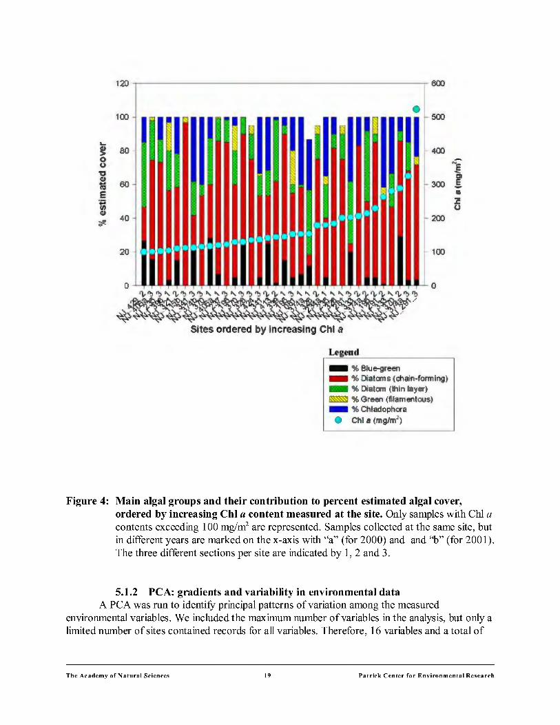
Main algal groups and their contribution to percent estimated algal cover, ordered by increasing Chl a content measured at the site . . . . . . . . . . . . . . . . . . 19

PCA including 24 sites and 16 variables sampled in 2000 and 2001 .......... 20

Correlations ofO-P and TP with Chl a concentrations ................... 21

DCA showing site scores ......................................... 26

CCA of diatom assemblage scores .................................. 27

Observed versus predicted TP for the W A inference model developed based on 85 diatom samples collected in 2000 ................................. 29

Test ofTP inference model: plot of measured versus diatom- inferred TP ..... 30

Scatterplot of measured 0-P versus the indices calculated by Specific Polluosensitivity index (IPS) for a112000 and 2001 samples ............... 33

Map showing the difference in the ratings of river quality as calculated by two European diatom indices, the Specific Polluosensitivity index (IPS) and the Biological Diatom Index (IBD) ..................................... 34

Box-plots comparing diatom inferred TP to AMNET macroinvertebrate impairment ratings .............................................. 39

The Academy of Nat ural Sciences vii Patrick Center for Environmental Research

List of Abbreviations

AFDM AMNET ANSP boot CCA Chla DCA IBI NAWQA NJDEP 0-P PCA PCER RBA RMSEP SWQS TN TKN TP USGS U.S. EPA WA

ash free dry mass Ambient Biomonitoring Network The Academy ofNatural Sciences, Philadelphia bootstrapped Canonical Correspondence Analysis chlorophyll a Detrended Correspondence Analysis index ofbiotic integrity National Water-Quality Assessment New Jersey Department of Environmental Protection orthophosphate Principal Component Analysis Patrick Center for Environmental Research rapid bioassessment root mean square error ofprediction Surface Water Quality Standards total nitrogen total Kjeldahl nitrogen total phosphorus United States Geological Survey United States Environmental Protection Agency weighted averaging

The Academy of Nat ural Sciences viii Patrick Center for Environmental Research

1 Introduction

Nuisance levels of algae in New Jersey (NJ) rivers and streams result primarily from high levels of inorganic nutrients coming from a variety of natural, agricultural, residential and urban sources. Excessive algal growth can cause water quality problems and can harm the designated use ofrivers and stream in different ways (Dodds and Welch 2000, U.S. EPA 2000b, ENSR 2001). Nutrient enrichment has been shown to increase benthic algal biomass in rivers through addition ofboth nitrogen and phosphorus (Blum 1956, Francoeur 2001). Many recent studies focus on understanding the effect of nutrient enrichment on excessive periphyton growth in rivers in order to develop management strategies for stream and river eutrophication (Dodds and Welch 2000, Dodds et al. 2002, Biggs 2000, Smith et al 1999).

Nationwide there is a continuous discussion concerning the establishment of nutrient limits and thresholds; their implementation is different from state to state. The U.S. EPA technical guidance manual for rivers and streams (U.S. EPA 2000a) recommends three approaches for development of nutrient and algal criteria: (1) the use of reference streams, (2) applying predictive relationships to select nutrient concentrations that will result in appropriate levels of algal biomass and (3) developing criteria from thresholds established in the literature. Also, in the Ambient Water Quality recommendations for U.S. EPA Rivers and Streams Aggregate Nutrient Ecoregion IX (U.S. EPA 2000b), U.S. EPA recommends establishing nutrient reference conditions in rivers and streams, using two methods: 1) establishing reference conditions based on the upper 25th percentile (75th percentile) of all nutrient data from all reaches sampled, or 2) determining the lower 25th percentile of the population of all streams within a region. A review of this approach for the New England Interstate Water Pollution Control Commission revealed that the ranges of predicted biomass production responses to nutrients, as tested for the subecoregions 59 and 84, would be below consensus threshold values (ENSR 2001). Nevertheless, the establishment of reference conditions based on percentiles will set different threshold values in different regions, depending on the range of overall water quality in the rivers of each particular region. These thresholds will be too high in ecoregions with rivers having predominantly high nutrient concentrations as compared to ecoregions with mainly low nutrient rivers and vice versa. The applicability of this method to the NJ Piedmont ecoregion needs further review. In this study, we apply the proposed U.S. EPA percentile method to the NJ Northern Piedmont dataset, in order to calculate reference conditions. We compare our results to the suggested Level III Subecoregion 64 reference conditions, Ecoregion IX (U.S. EPA 2000b) (see Discussion).

The current NJ Surface Water Quality Standards (SWQS) N.J.A.C. 7:9B-1.14(c) state that ''phosphorus as total P shall not exceed 0.1 (mg/L) in any stream, unless it can be demonstrated that total Pis not a limiting nutrient and will not otherwise render the waters unsuitable for the designated uses." (NJ DEP 2001). The SWQS further state as a nutrient policy, N.J.A.C. 7:9B-1.5(g)2: "Except as due to natural conditions, nutrients shall not be allowed in concentrations that cause objectionable algal densities, nuisance aquatic vegetation, or otherwise render the waters unsuitable for the designated uses." Therefore, current NJ Surface Water Quality Standards are recommending a threshold of0.1 mg/L TP in streams. Nevertheless,

The Academy of Nat ural Sciences Patrick Center for Environmental Research

the validity of this threshold value and the impact of nutrient inputs on algal growth in NJ rivers has not been studied in detail. The NJ DEP therefore needs a better understanding of the impact of the nutrients nitrogen and phosphorous on river and stream systems. Furthermore, nutrientalgal biomass relationships need to be investigated in more detail to develop alternative nutrient criteria and thresholds that can be applied to the state's rivers and streams.

The state ofNJ monitors river quality through an extensive Surface Water Quality Monitoring Network, originally measuring chemistry parameters 5 times a year at 200 stations from 1976 to the mid 1990s. Since 1997, 115 stations are measured 4 times a year statewide (NJ DEP 2000). Also, biological indicators are used to monitor river health through the state's Ambient Biomonitoring Network (AMNET) established in 1992. AMNET is an extensive network of 820 stations statewide. Macroinvertebrates are used to assess the biological impairment and geomorphologic conditions ofNJ rivers (NJ DEP 2000). Macroinvertebrates are widely used as indicators for organic pollution (Barbour et al. 1999), but they do not reflect inorganic nutrient levels well (Kelly and Whitton 1998, Schwoerbel1999). Therefore the NJ DEP has a need for application of different additional biological indicators to assess eutrophication and relationships between nutrient conditions and related excessive algal growth in NJ streams.

Algae, especially diatoms, are known to be good indicators of water quality and have been used in the United States since the 1950s (Patrick 1951). Algae are important ecosystem components and they are widely distributed in many habitats. The main advantages of using diatoms as indicators are the following: taxa are numerous and large numbers of individuals can be collected easily; diatoms can be identified to the lowest taxonomic level and strongly correlate with environmental characteristics; they are sensitive to stress, and respond rapidly to environmental change; and fmally, they can be stored efficiently. For all these reasons diatoms are valuable and cost-effective indicators for monitoring water quality (Barbour et al. 1999, Dixit et al.1992, Stevenson and Pan 1999).

This study was designed as a two-year project, initiated in July 2000. The purpose of this project was to develop algal indicators of stream and river eutrophication that can be applied in a regulatory context as secondary criteria for identifYing nutrient impairment. These indicators are based on relationships between extant water quality criteria (e.g., phosphorus and nitrogen concentrations) and overt signs of eutrophication. They are based on an understanding of algal dynamics in New Jersey streams, and help to distinguish between situations in which nutrient concentrations are high due to natural environmental conditions and those that result from anthropogenic influences.

The Academy of Nat ural Sciences 2 Patrick Center for Environmental Research

2 Study hypotheses, goals and approach

Hypotheses:

Goals:

This study is based on the following working hypotheses:

1) nuisance levels ofbenthic algal growth in NJ Piedmont rivers are caused by high concentrations of nutrients, especially phosphorus and nitrogen;

2) benthic algal biomass and species composition can be used as indicators of levels and causes of ecological impairment, primarily those related to the nutrients phosphorus and nitro gen.

To address these working hypotheses, the general objectives ofthis study were to:

1) explore the relationships between algal biomass as well as algal species composition and nutrients;

2) develop and test algal indicators of nutrients and water quality applicable to NJ Piedmont rivers;

3) make recommendations to the NJ DEP as to which indicators are best for monitoring nutrient impairment in NJ Piedmont rivers.

Approach:

In order to meet these objectives, the following approach was used in the analysis of the collected data.

1) First, all data were assembled in a database and files were created for data analysis and to present basic data in tables and appendices.

2) We examined site environmental data and created tables. We ran a PCA of environmental variables to understand the relative importance of major gradients and variability among sites.

3) The algal biomass data were summarized and characterized. Basic data were prepared in tables, graphics and appendices, and statistical programs were used to do correlations and regressions among the different measures and to determine how well they agree with each other.


4) The relationships among algal biomass measures and environmental characteristics, especially nutrients, were evaluated. We used ordination and correlation techniques to evaluate the potential for predictive relationships between nutrients, other environmental characteristics and algal biomass.

5) Biomass indicators of nutrient concentrations were developed and evaluated using simple and multiple regressions.

6) The relationships among algal species composition and environmental characteristics, especially nutrients, were evaluated using ordination methods and regressions with diatoms and soft-algae groups.

7) We developed and evaluated species composition-based indicators of nutrient concentrations. We used indicator taxa, simple metrics, European metrics, inference models, a Northern Piedmont TP model and other metrics/indicators.

8) Potential indicators for estimating algal biomass and for inferring relative phosphorus concentrations and overall water quality were compared.

9) Based on our results, we recommended the optimal set of available indicators for use in a monitoring program.


3 Study area

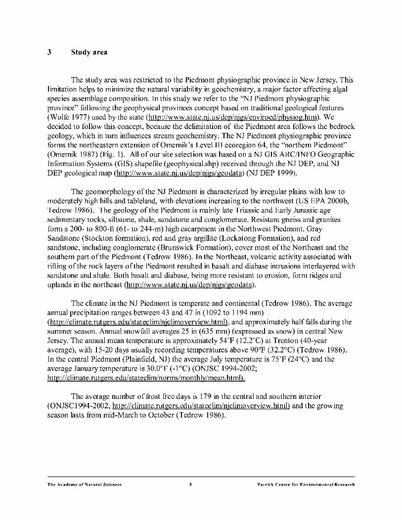
The study area was restricted to the Piedmont physiographic province in New Jersey. This limitation helps to minimize the natural variability in geochemistry, a major factor affecting algal species assemblage composition. In this study we refer to the ''NJ Piedmont physiographic province" following the geophysical provinces concept based on traditional geological features (Wolfe 1977) used by the state (http://www.state.nj.us/dep/njgs/enviroed/physiog.htm). We decided to follow this concept, because the delimitation of the Piedmont area follows the bedrock geology, which in turn influences stream geochemistry. The NJ Piedmont physiographic province forms the northeastern extension ofOmernik's Level III ecoregion 64, the "northern Piedmont" (Omernik 1987) (Fig. 1). All of our site selection was based on a NJ GIS ARC/INFO Geographic Information Systems (GIS) shapeftle (geophysical.shp) received through the NJ DEP, and NJ DEP geological map (http://www.state.nj.us/dep/njgs/geodata) (NJ DEP 1999).

The geomorphology of the NJ Piedmont is characterized by irregular plains with low to moderately high hills and tableland, with elevations increasing to the northwest (US EPA 2000b, Tedrow 1986). The geology of the Piedmont is mainly late Triassic and Early Jurassic age sedimentary rocks, siltstone, shale, sandstone and conglomerate. Resistant gneiss and granites form a 200- to 800-ft (61- to 244-m) high escarpment in the Northwest Piedmont. Gray Sandstone (Stockton formation), red and gray argillite (Lockatong Formation), and red sandstone, including conglomerate (Brunswick Formation), cover most of the Northeast and the southern part of the Piedmont (Tedrow 1986). In the Northeast, volcanic activity associated with rifting of the rock layers of the Piedmont resulted in basalt and diabase intrusions interlayered with sandstone and shale. Both basalt and diabase, being more resistant to erosion, form ridges and uplands in the northeast (http://www.state.nj.us/dep/njgs/geodata).

The climate in the NJ Piedmont is temperate and continental (Tedrow 1986). The average annual precipitation ranges between 43 and 4 7 in ( 1092 to 1194 mm) (http://climate.rutgers.edu/stateclim/njclimoverview.html), and approximately half fulls during the summer season. Annual snowfall averages 25 in (635 mm) (expressed as snow) in central New Jersey. The annual mean temperature is approximately 54 0F (12.2°C) at Trenton (40-year average), with 15-20 days usually recording temperatures above 90°F (32.2°C) (Tedrow 1986). In the central Piedmont (Plainfield, NJ) the average July temperature is 7YF (24°C) and the average January temperature is 30.0°F ( -1 °C) (ONJSC 1994-2002; http:/ I climate.rutgers. edu/ stateclim/norms/monthly/mean.html).

The average number of frost free days is 179 in the central and southern interior (ONJSC1994-2002, http://climate.rutgers.edu/stateclim/njclimoverview.html) and the growing season lasts from mid-March to October (Tedrow 1986).


Pennsylvania

flllllllllll N.J Pledmonc c::::::::l sludv area

Figure 1: Location of the NJ Northern Piedmont physiographic province within Omernik's Level III ecoregion 64, the "northern Piedmont."

Landuse in the NJ Piedmont is primarily a mix of farmland and urban areas. The urban and industrial areas are concentrated in the northeastern, and to a lesser degree, the southwestern portion of the Piedmont. Nutrient inputs into the rivers of the NJ Piedmont come from a variety of natural, agricultural, residential and urban sources and make this area an ideal region to investigate impacts of nutrient input from different sources. The rivers and streams of this area fall within the U.S. EPA Rivers and Streams Aggregate Nutrient Ecoregion IX, the southeastern temperate forested plains and hills. This Aggregate Ecoregion contains 11 subecoregions, including the Northern Piedmont as subecoregion 64 (Omernik's Level III ecoregion) (US. EPA 2000b ). The rivers in this subecoregion have relatively high nutrient concentrations. The median total phosphorous (TP) values, calculated over one decade, range from 2.5 to 1760 ).lg/L, with a summer mean of 150 ).lg/L and a median of 70 ).lg/L. Median total nitrogen (TN) values range from 0.5 to 12 mg/L with a summer mean of 4.8 mg/L and a median of 4.2 mg/L (U.S. EPA 2000b).


4 Methods

4.1 Site selection

We selected an initial set of30 study sites to be sampled in fall2000 in cooperation with NJ DEP staff, mainly Tom Belton. Because a goal of this study was to develop algal indicators of anthropogenic nutrient increases, it was important to select a suite of sites with relatively similar natural environmental conditions, but with a wide range of nutrient concentrations. The sites are restricted to the Piedmont physiographic province in northern New Jersey, and have a relatively limited range of hydrology, morphology and substrate type. This limitation helps to minimize the variability in geochemistry, a major factor affecting algal species composition. In addition, we used nutrient concentration data from the NJ DEP as an indication of watershed sources of anthropogenic phosphorus and nitrogen. For all sites, chemistry data were available either through the NJ monitoring network program or through the USGS for their monitoring stations. All sites are part of the NJ Ambient Monitoring Network. We selected sites with a range of impairment from no impairment to severe impairment, based on AMNET Macroinvertebrate classifications made in 1992/93 and 1998/99 (Table 1). About one-third ofthe selected sites were studied in the same year (2000) by the NJ DEP to develop a fish IBI. Three sites (AN0215, AN0318 and AN0321) sampled during 2000 were accidentally located in the Highlands and two sites (AN0382, AN0439) were sampled in the Inner Coastal Plains physiographic provinces (Fig. 2), due to initially inaccurate interpretation of the NJ Piedmont province delimitation. This error was corrected later, and the samples were excluded from development of indicator metrics.

During the second study year (200 1) we selected 13 sites (in cooperation with NJ DEP staff), classified in three categories: 1) "new sites" to fill in data gaps in the gradient of phosphorus concentrations, and to supplement the "calibration" set chosen during the first year, 2) "test sites" to evaluate indicators developed during the frrst year and, 3) "duplicate sites" to investigate variation in algal biomass and diatom assemblage composition between years one and two. Selection criteria were the same as those used during year one with an altered focus within each category: "new sites" have high concentrations ofTP (as recorded by the NJ DEP and/or USGS). "Test sites" cover a range from no- to severe-impairment based on AMNET results and have a USGS gaging station. We selected as "duplicate sites," AMNET sites with severe impairment in 1998 and/or that were planned to be Fish IBI sites in 2001 (see Table 2).

All rivers selected for both years are 1st to 6th order wadeable streams. The classification is based on information from the NJ DEP' s GIS hydrography stream network line shape files for New Jersey counties, generated as line Arclnfo coverages from USGS 1:24,000 Digital Line Graph (DLG) files (http://www.state.nj.us/dep/gis/GIS maps). The sites sampled are located in the following USGS Watershed Management Areas: Central Delaware, Millstone, Lower Raritan, North and South Branch Raritan River, Upper Passaic, Whippany and Rockaway, Arthur Kill, Lower Passaic and Saddle, Hackensack and Packsack and Pompton, Wanaque and Ramapo. Most of them are located in Somerset, Morris and Bergen counties, and a lesser portion are distributed over Mercer, Hunterdon, Middlesex, Union, Passaic and Essex counties.


Legend

• 2000 sites 2001 sites

37238 • 231

Figure 2: Site locations in the Piedmont physiographic province of New Jersey for sampling years 2000 and 2001. Site numbers correspond to New Jersey AMNET site location IDs. See Tables 1 and 2 for site names and locations.


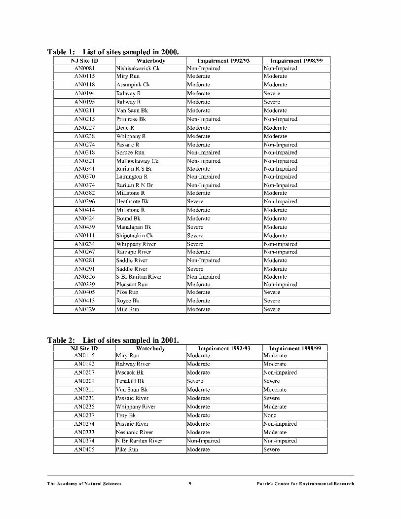
Table 1: List of sites sam led in 2000. NJ Site ID I Water body I Impairment 1992/93 I Impairment 1998/99

AN0081 INishisakawick Ck IN on-Impaired IN on-Impaired AN0115 IMiryRun !Moderate !Moderate

AN0118 IAssunpink Ck !Moderate !Moderate

AN0194 IRahwayR !Moderate !severe

AN0195 IRahwayR !Moderate !Severe

AN0211 IVan SaunBk !Moderate !Moderate

AN0215 I Primrose Bk IN on-Impaired IN on-Impaired

AN0227 IDeadR !Moderate !Moderate

AN0238 IWhippanyR !Moderate !Moderate

AN0274 !Passaic R I Moderate !Non-Impaired AN0318 !Spruce Run IN on-Impaired IN on-Impaired

AN0321 I Mulhockaway Ck IN on-Impaired IN on-Impaired AN0341 !Raritan R S Br !Moderate IN on-Impaired AN0370 I Lamington R IN on-Impaired IN on-Impaired

AN0374 I Raritan R N Br IN on-Impaired IN on-Impaired AN0382 I Millstone R !Moderate !Moderate

AN0396 I Heathcote Bk !severe IN on-Impaired

AN0414 I Millstone R !Moderate !Moderate

AN0424 IBoundBk !Moderate !Moderate

AN0439 !Manalapan Bk I severe !Moderate

ANOlll I Shipetaukin Ck !severe !Moderate

AN0234 !Whippany River I severe IN on-impaired AN0267 !Ramapo River !Moderate IN on-impaired

AN0281 I Saddle River IN on-Impaired !Moderate

AN0291 I Saddle River I severe I Moderate AN0326 IS Br Raritan River IN on-Impaired I Moderate AN0339 I Pleasant Run I Moderate IN on-impaired AN0405 I Pike Run !Moderate I severe

AN0413 !Royce Bk !Moderate !severe

AN0429 I Mile Run !Moderate I severe

Table 2: List of sites sam led in 2001. NJ Site ID I

AN0115

AN0192 !Rahway River !Moderate !Moderate

AN0207 IPascack Bk !Moderate IN on-impaired

AN0209 ITenakill Bk I severe I severe

AN0211 IVan SaunBk !Moderate !Moderate

AN0231 !Passaic River !Moderate !Severe

AN0235 !Whippany River !Moderate !Moderate

AN0237 !Troy Bk !Moderate IN one

AN0274 !Passaic River !Moderate IN on-impaired

AN0333 !Neshanic River !Moderate !Moderate

AN0374 IN Br Raritan River IN on-Impaired IN on-impaired

AN0405 IPike Run !Moderate I severe


4.2 Sampling period

During both years, samples were collected by ANSP staffMike Hoffmann, Diane Winter and Karin Ponader from August through October. The first year sites were sampled from 9 August through 3 October 2000. In the second year, sampling was completed between 20 and 26 August 2001. During the 2000 field season, sampling was suspended for two weeks to wait for rivers to recover from the scouring effect of high flow conditions caused by very heavy rainfall events during the second week in August. We chose to sample in late summer because the influence of higher streamflow velocity and discharge on algal assemblage composition is lowest during this period. Based on the average of monthly mean streamflow calculated for 77 years (since 1925), the lowest flow records in NJ rivers were measured in August, September and October (http://www.waterdata.usgs.gov). Samples collected during this time are also most directly comparable with sample data from other studies conducted in the area, such as the National Water-Quality Assessment Program (NAWQA), the EPA Riparian Reforestation Project and the Growing Greener Project all conducted at the PCER (http://www.acnatsci.org/research/pcer/projects.html). All these projects were conducted at the ANSP and follow USGS NAWQA Periphyton sampling protocols recommending sampling periods to be conducted during normaL low- or stable-flow periods (Moulton et al. 2002, Porter et al. 1993).

4.3 Collection of samples/data

4.3.1 Site characterization/establishment of sampling reaches All sites sampled are located at NJ DEP AMNET monitoring stations, which are defined

as the intersection of a road and the river to be sampled. According to NJ DEP field sampling protocols, we sampled on the upstream side of the bridge to minimize the effect of inputs from automobile use/traffic and street maintenance. Some exceptions were made at sites where conditions did not allow sampling upstream and where the downstream side was considered more representative of the river habitat. Prior to collection of water chemistry and algal samples, we took detailed notes on general physical site characteristics, geomorphology, weather conditions, overt signs ofhuman impact, etc. The sampling area was divided into three sampling reaches, so that variability among different sections ofthe rivers could be assessed. The three sections were determined using the following criteria: each section should contain a minimum of2 riffies and 2 pools and the length of each reach should be approximately 10 times the channel width. Commonly used guidelines (Fitzpatrick et a1.1998) recommend a minimum reach length of 150m for wadeable streams. We did not follow these guidelines and established shorter reaches because of the generally smaller width of the rivers sampled in the NJ Piedmont area. The average width of the rivers sampled was 13 m (range of 3-50 m) and the average length of the established sampling reaches was 44 m (see Appendix 1a). We believe our criteria were satisfactory for establishing reaches that represented the local variability within the river. Once the reaches were established, we recorded information on all three sections, made site drawings, and measured the physical characteristics of the sampling sites. Sites are documented with digital images (Sony MVC-CD1000), burnt on a CD and submitted to the NJ DEP. For each section, we made a visual


estimate of percent substrate type (boulder, cobble, gravel, sand, silt, bedrock) and flow velocity. Light conditions (percent open canopy cover) were measured using a spherical densiometer.

4.3.2 Water chemistry samples Water chemistry samples were taken prior to algal sampling to avoid disturbance of the

water column and sediments. Samples were taken using a plastic syringe with an attached filtration device. Laboratory analysis ofN03-N, NH3-N, 0-P and TP was performed by the PCER Geochemistry Section (V elinsky 2000). In 2001, we took additional samples for analysis of chloride, total alkalinity, total hardness and conductivity. Samples were cooled immediately on ice in the field and shipped to the ANSP where samples for nutrient analysis were frozen immediately. Results ofthese analyses were used to supplement those collected by the NJ DEP. Samples collected directly by ANSP in the field better represent conditions near the time that algal samples were collected, and provide information ofthe nature and magnitude of variation in water chemistry.

4.3.3 Diatom and biomass/soft algae samples Samples were collected from natural rock substrates using techniques consistent with

those used in the USGS NAWQA program (Moulton et al. 2002) and the EPA Rapid Bioassessment protocols for periphyton (Barbour et al. 1999). All sampling procedures are documented in a PCER protocol (Charles et al. 2002). Two types of samples were taken. One, a composite diatom sample, was created by randomly selecting 4-5 rocks of ca. 5 em diameter. The rocks were carefully selected from mid-stream and were free of visible filamentous algae. In 2000, samples from sticks, gravel or sand were collected at five sites where no rocks were available (AN0194, AN0227, AN0238, AN0382, AN0414). Algae were removed from the rocks by scraping and brushing, placed in plastic containers and preserved in the field by keeping them on ice in a cooler. The second type of sample was a quantitative composite biomass sample collected for measurement of chlorophyll a and ash-free dry mass (AFDM). These samples were analyzed by the Patrick Center for Environmental Research's (PCER) Geochemistry Section. Three bigger rocks (with an average diameter of ca.1 0 em) were selected randomly to represent the distribution of algal coverage within each reach section. Rock surfaces were scraped, and outlines of rocks were drawn on waterproof paper. Surface area was measured using an aluminum foil method (Moulton et al. 2002, Ennis and Albright 1982). NJ DEP guidelines were followed for preservation and storage ofChl a samples. All samples (diatoms and Chl a) were preserved by keeping them on ice in a cooler and were shipped to the ANSP over night for immediate treatment in the laboratory the next morning. In total, 85 diatom samples were taken during 2000. Only 71 samples were collected for biomass in 2000; biomass samples were not collected at 6 sites with sandy substrate. In 2001, we only sampled rock substrate, collecting 35 diatom and biomass samples in total. Both year's datasets combined contain a total of 120 diatom samples and 106 biomass samples.

4.3.4 Visual biomass estimate (EPA rapid bioassessment protocol) In addition to algal sample collection, the percent cover and thickness of algal growth was

measured using the Rapid Periphyton Survey Method (EPA Rapid Bioassessment Protocol) developed by the U.S. EPA (Barbour et al. 1999). This method provides a quantitative estimate of


filamentous and other types of algae that often have patchy distributions and whose biomass is difficult to quantifY. For each sampling section, we measured percent biomass cover for each algal group along three transects across the river. Length of filamentous strains and thickness of algal mats per algal group were also recorded. For each section, an average was calculated from the three transects and used in data analysis. We collected additional samples for algal identification and examination under the microscope when identification in the field was not possible.

4.3.5 Additional data (water chemistry, landuse) In addition to the water chemistry and biomass data produced at the PCER, all other data

were provided by the NJ DEP through Tom Belton. Landuse data for each watershed were assembled by Jack Pflaumer (NJ DEP). Also, Jack Pflaumer sent ANSP most of the additional chemistry data records collected by USGS and NJ DEP at the surface water monitoring stations. He assembled available data for the sampled periphyton sites for each sampling year. Additional data were retrieved by Karin Ponader through the USGS "water quality samples for USA" webpage (http://www.waterdata.usgs.gov/nwis/qwdata) and the NJ 2001 Water-Resources Data report (Reed et al. 2002). Because sampling was not necessarily done at the same time by USGS and PCER staff, all USGS/NJ DEP data used in our analysis were measured within a maximum of 4 weeks from algal sampling in the same year.

4.4 Algal sample preparation and analysis

Samples were prepared for algal analysis using standard protocols (Velinsky and DeAlteris 2000). Chlorophyll a and ash-free dry mass (AFDM) samples were analyzed by the PCER Geochemistry Section using methods as described in Standard Methods and US EPA method 445 (APHA, AWWA AND WPCF 1992, U.S. EPA 1992). Diatoms were permanently mounted on microscope slides following routine protocols (Charles et al. 2002). A total of 85 slides was prepared for year 1 and a total of35 slides was prepared for year 2. Per slide, 600 valves were identified to lowest taxonomic level and counted using USGS NA WQA protocols (Charles et al. 2002). Identification was done using common taxonomic references available at the ANSP as well as type material from the ANSP Diatom Herbarium. Over 900 digital images were taken, recording nearly all identified and unidentified taxa. Taxonomic problems were discussed with PCER Phycology Section members, and problematic and unknown species were described and recorded in the ANSP Algae Image database (http://diatom.acnatsci.org). Also, the active participation ofKarinPonader in the Fourth through the Eighth NAWQA Taxonomy Workshops on Harmonization of Algal Taxonomy held at the Academy ofNatural Sciences in October 2000, June and October 2001 and May and October 2002 helped in solving taxonomic issues in the NJ Piedmont diatom flora.

Diatoms were counted and recorded directly into a database using the computer pro gram Tabulator, version 3.7.0 (Cotter 1999-2000, Cotter 2001). Count reports are created for each count, including information on assemblage composition, taxonomic notes, etc. The common filamentous algae were identified and semi-quantitative estimates were made of their abundance using a new count method developed specifically for this project (Ponader and Winter 2002). This semi-quantitative procedure is designed to provide percentage estimates of the most common


species of algae that make up the largest proportion of the algal biomass for each sample. The method consists of two steps. The frrst step involves identifYing the most common genera/species and estimating the relative percentage of each of these in the algal assemblage. In the second step, the relative percentage that each genus/species contributes to the algal biovolume in the sample is estimated. Because this is a semi-quantitative method, cells are not counted or measured, but a general estimate is made, which describes the relative proportions of the common genera and species observed in the sample through examination of several transects.

4.5 Data storage and documentation

All data collected during this project were properly stored in the PCER Phycology section's database management system, the North American Diatom Ecological Database (NADED) using Microsoft Access 2000. The field sheets were scanned and all digital images of sites and samples were burnt on CDS. Copies are available on request. All image documentation and site information were archived in the database.

4.6 Data analysis

4.6.1 Water chemistry: PCA to explore gradients and variability among sites Prior to examining the relationships among algal biomass, species composition and

environmental variables, we performed a Principal Component Analysis (PCA) using Canoco for Windows version 4.02 (ter Braak and Prentice1998). The environmental variables were centered and standardized. The aim of running a PCA was to discover the principal patterns of variation within the environmental variables measured and how they relate to sampling sites. Outliers were defined as samples with scores falling outside the 95% confidence limit about the sample score means in a PCA of the environmental variables (Hall and Smol1992, Birks et al. 1990b).

4.6.2 Algal biomass

4.6.2.1 Spearman's rank-order correlation (correlations between nutrients, algal biomass and algal species composition)

A Spearman's rank-order correlation was run using the program SPSS version 11.0 for Windows. We chose to run this analysis because many of the algal biomass variables listed below are not measured on a continuous scale and none ofthemhad normal distribution (Dytham 1999). Included in this analysis were the following data for all1 06 samples collected during both years: Chl a and AFDM data, nutrient measurements (TP, 0-P, NH3-N, N03-N), percent open canopy cover and substrate type, soft algal species composition data obtained through the semiquantitative analysis for all 106 samples, as well as different measures of algal biomass. The latter were created through combination of different categories, e.g., different algae types and their abundances multiplied by estimated algal thickness and length rank. In total, 110 variables and combinations of variables/categories were used in the analysis. Because of the size of the complete report file (over 100 pages) we only list here (Appendix 3) the results of a reduced set of 67 selected variables, excluding the combinations (e.g., algal type multiplied with length rank


or thickness etc.). The results of the strongest and most significant relationships are listed in sections 5 .2.1.1 and 5 .2.2.2.

4.6.2.2 Forward stepwise regression (analysis of principal factors influencing algal biomass)

To help determine the principal factors influencing algal biomass, we examined correlations among algal biomass, nutrients, geomorphology and light conditions, running a Forward Stepwise regression with Sigma Stat 2.03. All chemical variables (except pH) were loglO transformed. The substrate categories were analyzed both separately and combined into different categories. We separated bigger hard substrate types into two categories, one including only bedrock and boulder and the other containing cobble and gravel. We created two other categories, one including all bigger substrate from bedrock to gravel and another combining all smaller and soft substrate (sand, silt and clay).

4.6.3 Diatom assemblages Numerical analyses were performed to investigate the factors affecting diatom species

composition, and to determine whether species composition was influenced by nutrients strongly enough to justify development of inference models. We used Canoco for Windows version 4.02 (ter Braak and Prentice1998) to perform these analyses. Because their distributions were skewed, we log 10 transformed all water-quality variables included in the analysis, except pH. All diatom species identified in the counts from all the sites sampled in 2000 were included in the ordinations.

4.6.3.1 Detrended Correspondence Analysis (DCA) to determine principal patterns of variation in diatom species composition

A detrended correspondence analysis (DCA) was performed to determine the gradient length as a measure of the maximum amount of variation in the diatom data. The gradient length was 2.6 for the first axis, exceeding the value of 2 standard deviation (SD) units, recommended as the point above which unimodal techniques should be used for further analysis and development of calibration sets (Jongmann et al. 1995, ter Braak and Prentice 1998). In the same DCA ofthe species data, outliers were determined as samples with sample scores falling outside the 95% confidence limit about the sample score means (Hall and Smol1992).

4.6.3.2 Data screening: environmental variable with extreme influence on species composition

All methods for screening data to remove outliers prior to developing diatom inference models follow standard procedures used in several publications (Fallu et al. 2000, Hall and Smol 1992, Winter and Duthie 2000). In our study, after outliers were determined in a PCA of the environmental variables and/or in a DCA of the species data (see sections 4.6.1. and 4.6.3.1), the second step was to delete samples that had an environmental variable with an extreme influence other than either TP, 0-P, N03-N or NH3-N on the diatom species composition (Birks et al. 1990b, Hall and Smol1992). In this case, samples were deleted if their residual length on the environmental variable axis fell outside a 95% confidence limit as detected in a CCA constrained to the variable to be reconstructed (Hall and Smol1992).


4.6.3.3 Ordination analysis: CCA (influence of environmental variables on diatom species composition)

To identify the variables that explained a significant amount of variation in diatom species composition and that had an independent influence on diatom species distribution, we ran a series ofCCAs constrained to one variable at a time. We calculated the ratio of the sum of the first constrained eigenvalues (A. 1) to the sum of the second unconstrained eigenvalues (A.2). The variables with highest values of A1 /A.2 were selected as likely to have the most influence on diatom species distribution (Winter and Duthie 2000). Also, as part of the same CCAs that were constrained to one variable, the statistical significance of each variable on the first canonical ordination axis was evaluated using Monte Carlo permutation tests (199 permutations, p:0: 0.05) (Fallu et al. 2000). Variables that did not explain a significant amount of variation in diatom composition were excluded from the dataset used for development of inference models.

4.6.3.4 W A-regression and calibration (development and testing of nutrient inference models)

Nutrient inference models were developed with weighted averaging (W A) regression and calibration techniques using WACALIB version 3.5 (Birks 2001, Line et al. 1994). Diatom species optima and tolerances were calculated for the nutrient variables TP, 0-P, NH3-N and N03-N. The models included all diatom species. Species abundance(%) was transformed by calculating the square root of each value. Species tolerances were corrected by deshrinking with an inverse regression procedure (ter Braak and van Dam 1989). We used bootstrapping (1 OOOx) (Birks et al. 1990b) to estimate the root mean square error of prediction (RMSEP) of each model developed. The predictive power of the developed models was assessed based on the r(bootland the RMSEP(boot). The model with the highest predictive power and the lowest RMSEP is the best model calculated. To evaluate the performance of the TP model developed, we tested them on samples collected in 2001, performing WA-calibration using CALIBRATE version 0.61 (Juggins and ter Braak 1997, Juggins and ter Braak 2001). The performance of the model applied was assessed using statistics describing the correlation between the observed versus inferred values (Birks et al. 1990b).

4.6.4 Calculation of diatom metrics

4.6.4.1 Diversity metrics and other simple metrics Diatom diversity indices and other simple metrics were calculated using 98 diatom samples

from both years, following Barbour et al. (1999). We calculated the number of diatom taxa in the sample(# Taxa), the Shannon-Weiner diversity index (S-W Index), the percent oftotal diatom valves made up of taxa that occurred in> 10% abundance (Percent Dominants), the percent of total diatom valves made up by the most abundant taxon (% Dominant Taxon), the ratio Centrales /Pennales C/P), and finally, the Siltation Index(% Siltation Index), which is the sum of the percent abundances of all species in the genera Navicula, Nitzschia, Cylindrotheca, and Surirella. These are common genera of predominantly motile taxa that are able to maintain their positions on the substrate surface in depositional environments (Bahls 1993). We evaluated the use of these


indices in conjunction with different types oflanduse, running a Spearman's rank-order correlation using Sigma Stat 2.03.

4.6.4.2 European diatom indices Twelve different diatom indices, widely used in Europe, were calculated for the NJ diatom

dataset. In our study we were specifically interested in the results of the Trophic Diatom Index (TDI) (Kelly and Whitton 1995, Kelly 1998), mainly reflecting nutrient conditions (especially TN and TP), as well as in the Biological Diatom Index (IBD) (Prygiel and Coste 1999) and the Specific Polluosensitivity index (IPS) (Coste in Cemagref 1982), both reflecting overall impairment conditions. The calculations were done by Luc Ector (Centre de Recherche Gabriel Littmann, Luxembourg) with OMNIDIA, a program specifically designed for calculations of diatom indices (Lecointe et al. 1993 ).


5 Results

5.1 Environmental data

5.1.1 Water chemistry, biomass concentrations and summary of site characteristics

Table 3 summarizes the nutrient and biomass characteristics measured at all sites in both years. TN concentrations were calculated for 25 samples only, due to missing TKN measures in the available USGS data. For information on the full dataset used and all variables measured, see Appendices la and lb.

Table 3: Statistical summary of nutrient and biomass concentrations at all sampling sites. Data include 2000 and 2001 samples. TP, 0-P, N03-N, NH3-N, Chl a and AFDM were measured at the PCER. TN is calculated combining PCER data (N03-N) and USGS data (TKN available from 25 stations only).

Variable Minimum Maximum n samples

TP (mg/L) 0.15 0.07 0.01 1.30 41

0-P (mg/L) 0.11 0.04 <0.01 1.14 41

TN (mg/L) 2.13 1.77 0.89 5.74 25

N03-N (mg/L) 1.92 1.33 0.23 7.55 41

NH3-N (mg/L) 0.05 0.03 <0.01 0.18 41

Chi a (mg/nt) 109 81.0 2.19 1115 106

AFDM (g/m2) 20.5 12.7 3.80 153 106

Figure 3 shows TP and Chl a concentrations measured for both sampling years. The sites are ordered by increasing TP concentrations. In comparison, the sites sampled in 2001 have generally higher TP concentrations than in 2000, which was one of our goals when selecting sites for 2001. Comparison ofTP and Chl a values at sites that were resampled in 2001 does not show significant differences between both sampling years. Figure 3 also shows that Chl a values do not increase significantly with increasing TP, reflecting challenges of using Chl a as an indicator of increased nutrient contents. This is discussed further in the statistical analysis and the discussion. In our dataset, 46% of the samples that were collected from sites with concentrations of 0.1 mg/L ofTP in the water column show Chl a concentrations greater than 100 mg/m2

• The mean for all samples collected in 2001 and 2002 is 109 mg/m2 Chl a. Observations in the field have shown that samples with Chl a > 150 mg/m2 were taken from sites with extreme algal growth based on visual estimates.


800 ~--------------------------------------------~------~

600 ,.........

1: ........ Ol 00

E

200

0

• TP (mgll) Chi a median value/ lte (m 1m2

)

---- ChI a concentration of 100 mg 1m 2

••••••• ••••••••••••• ••••••••••

•

• • 0.8

0.6

,......... -........ C)

o.4 E

a.. 1--

Figure 3: TP and Chi a concentrations measured in 2000 and 2001. Sites ordered by increasing TP (black circles). At each site three Chl a measurements were taken (one per reach). Green circles represent median Chl a concentrations and error bars indicate maximum and minimum Chl a concentrations per site. Site numbers a and b indicate that sites were sampled in both years ( a=2000 and b=200 1 ).

The visual estimates of algal cover along transects (see description of method under section 3.3.4) are summarized in Figure 4. To highlight the major trends, only samples with Chl a concentration exceeding 100 mg/m2 are represented in this graph. Sites are ordered by increasing Chl a content. Estimates of filamentous algal cover showed that at most sites% estimated diatom (chain-forming) cover was most important, followed by% Cladophora. The third important group was % thin diatom cover, represented by thin diatom mats that do not form chains or filaments. Finally, % blue-green algae was the next most abundant cover, followed by % green algae cover. There was no clear correlation between percent visual estimate of algal cover of individual algal groups and measured Chl a. Therefore, we further investigated whether the visual estimate of total biomass shows any significant relationship with measured biomass (Chl a and AFDM) using correlation analyses as described in section 5.2.


120

100

'-

~ 80 0 u "0 Ql

60 ... 1'01

E ~ Ql

~ 40 ..

20

600

500

400

300

200

100

0

% Blue-green % Diatoms (chain-form ing) %Diatom (thin layer) % Green (filamentous) % Chlad ophora

Chi a (m g/m)

-"'E 0, .5. til

:c 0

Figure 4: Main algal groups and their contribution to percent estimated algal cover, ordered by increasing Chi a content measured at the site. Only samples with Chl a contents exceeding 1 00 mg/m2 are represented. Samples collected at the same site, but in different years are marked on the x-axis with "a" (for 2000) and and ''b" (for 2001). The three different sections per site are indicated by 1, 2 and 3.

5.1.2 PCA: gradients and variability in environmental data A PCA was run to identifY principal patterns of variation among the measured

environmental variables. We included the maximum number of variables in the analysis, but only a limited number of sites contained records for all variables. Therefore, 16 variables and a total of


24 samples in 2000 and 2001 were included. The PCA shows that the sites are distributed along three main axes (Fig. 5). The percentage ofvariance explained by the first two axes was 54%, with eigenvalues of A. 1= 0.34 and A2 =0.20, respectively. Axis 1 reflected a gradient of several nutrients (TKN, TN, 0-P, TP, N03-N) and separated sites with low nutrient concentrations from sites with higher nutrient values. The second axis is mainly influenced by a combination of pH, basin size, DO, and DOC. This axis reflects mainly river width and related DOC loadings, separating narrower rivers with higher DOC loadings from wider rivers with lower DOC concentration. The third axis is influenced mainly by % urban, conductivity and % agriculture, showing that sites are mainly distributed along an urban gradient. Agriculture does not show a strong gradient, as most sites in the NJ Piedmont were sampled in urban areas. Generally, this analysis shows that the sites follow a strong nutrient gradient. The following samples were determined to be outliers: Sites AN0291 and AN0231 showed extreme 0-P, TP and N03-N concentrations. Site ANO 118 was identified to have extreme Chl a and nutrient values.

en 0

en 0

I

oFOREST

-1.0

I

pH BA IN SIZ~ 274 0

081

.

2098 ! 21 1 b

0 : 3 195 ! 192

iO ! I

!234 0 0

! 115 2 • •

DOC

2310

2910

TKN

NH3- N 'Yo RB- N

1.0

Figure 5: PCA including 24 sites (circles) and 16 variables (arrows) sampled in 2000 and 2001. Numbers represent the last three digits of the NJ site ID (see Table 1). The length of each arrow expresses the "strength" of the influence of the variable on site distribution. Each axis is determined by a combination of variables. The variables are color-coded corresponding to the axes: axis1 =blue, axis 2 =red, axis 3 =green.


5.2. Algal biomass

The different methods of assessing biomass in the field and in the laboratory produced a multitude of variables, all expressing algal biomass in a different way. One ofthe main goals of this studywas to identifY the strength ofnutrient-biomass relationships and their use for development of indicators. Therefore, we needed to know: a) How well do the different measures ofbiomass correlate? and b) How well does measured/estimated biomass reflect nutrient conditions? To answer both questions a Spearman's rank-order correlation was performed, as described below. The results are presented in sections 5.2.1.1 and 5.2.1.2, answering the above two questions. Finally, we explored how strongly other environmental factors influence algal biomass measures by running a Forward Stepwise regression.

5.2.1 Spearman's rank-order correlation Relationships among all nutrient variables and biomass data for the full data set from both

years' (n=106) data were explored using a Spearman's rank-order correlation matrix. To fmd out what type of correlation was appropriate to run, we needed to determine if variables in the dataset were normally distributed. We tested each variable using Kolmogorov-Smirnov (K-S) tests (Dytham 1999) using the procedure in Sigma-Stat 2.03. Normality tests failed for all variables when tested on untransformed data, showing that all data were skewed. After log transformation, another K-S normality test was run. The results showed that only Chl a (log) passed the test, and that the data were still skewed for most of the variables. Scatterplots using log transformed nutrient data (Fig. 6) show no significant trend in correlations ofO-P or TP with Chl a concentrations. Therefore we decided to run a Spearman's rank-order correlation, to investigate if nutrients showed a significant influence on biomass concentrations.

1200 •

1000 r 2 = 0.093

N 800 E ......_ Ul 600 • E • ltl 400

J: • 0

200

0 , . •

0.5 1.0 1.5 2.0 2.5

TP (IJg/1) log1 0

1200

1000

1: 800 ......_ Ul E

600

-ltl 400

J: 200 0

0

3.0 0.0

r' = 0.087

0.5 1.0

•

•

• •

• I .; • •

1.5 2.0 2.5 3.0

P04 (IJg/1) log1 o

Figure 6: Correlations of P04 and TP with 3 Chi a concentrations. All samples from 2000 and 2001 are included. P04 and TP values are log transformed.

The variables in the Spearman's rank-order correlation included all measures of algal biomass (Chl a and AFDM data, RBA visual estimate and semi-quantitative count procedure) for all106 samples collected during both years, and all nutrient measurements (TP, 0-P, NH3-N,


N03-N). For explanation of the different variables included in the correlation, and results of the correlation matrix, see Appendix 3. We used the following abbreviations to identifY the method or analysis from which the data were derived: Rapid bioassessment (RBA) and semi-quantitative count method (SQCM).

5.2.1.1 Comparison between results of different biomass measures/estimates (Chl a, AFDM, visual estimate (RBA) and % biomass estimate (semiquantitative count method)

The following correlations are significant at the 0.01level using Spearman's rank-order correlation, two-tailed test. Chl a is significantly correlated with% visually estimated Cladophora sp. cover (RBA) (r= 0.40), with visually estimated % Cladophora sp. cover multiplied by its length rank (RBA) r = 0.41), and with visually estimated% blue-green cover multiplied by its length rank (RBA) r = 0.26). In contrast, AFDM is not significantly correlated at the 0.01level (two-tailed) with any% biomass estimate. Correlations at the 0.05 level are more frequent but less strong showing the following results: Chl a correlates with estimated % Cladophora sp. biomass (SQCM) r =0.24), with % estimate blue-green algae cover (RBA) (r=0.25) and with estimated % cover of green algae (RBA) r =0.21). AFDM is correlated (at the 0. 05 level, twotailed) with estimated % Oegodonium sp. biomass (SQCM) (r=0.22), estimated % biomass green filamentous algae (RBA) ( r= 0.19), and estimated % biomass green filamentous algae multiplied by its maximum length rank (RBA) r =0.19). AFDM is negatively correlated with diatom estimated biomass (SQCM) r = -0.20), estimate of% thin layer of diatoms (RBA) (r= -0.19) and estimate of %thin layer of diatoms multiplied by their thickness rank (RBA) (r= -0.23).

In summary, the results of the Spearman's rank-order correlation show that both,% estimate of Cladophora sp. biomass (RBA) and % estimate of Cladophora sp. biomass multiplied by its length rank (RBA), and visually estimated % blue-green cover multiplied by its length rank (RBA) are the two groups that are correlated strongest and most significantly (at the 0.01 level) with Chl a. AFDM correlates with mainly Oegodonium sp. biomass (RBA) and cell counts (SQCM), and green filamentous algae thickness and maximum length (RBA), but the correlations are weaker and less significant. In general, biomass measures (Chl a and AFDM) show stronger correlations with the results of the RBA than with the semi-quantitative count method. This study shows that the Rapid Bioassessment method is a good tool to estimate biomass impairment in rivers ofNJ, and especially seems to reflect well extreme growths of Cladophora sp. Nevertheless, besides the correlation with Cladophora sp., none ofthe correlations is very strong and interpretations should be made with caution.

5.2.1.2 Relationships between algal biomass measures and nutrient conditions We explored the relationships between algal biomass measures and nutrient conditions

using Spearman's rank-order correlation, two-tailed test (Appendix 3). The only correlation that was significant at the 0.01level was a positive relationship between AFDM and nitrate (N03-N) r = 0.26), and a negative relationship between estimated% blue-green cover (RBA) r =-0.31) and estimated% blue-green cover multiplied by its thickness rank (RBA) r =-0.29) and NH4-N. In summary, except for AFDM and N03-N, we did not find significant trends or strong positive relationships between amount ofChl a, AFDM, visual biomass estimate and nutrient


measurements. The results of the data analysis performed during the frrst two years of our study reveal that nutrient concentrations measured in NJ Piedmont rivers do not show strong and significant correlations with any of the different biomass measures. However, the results of forward stepwise regression (section 5.2.2.) suggest that if the influence of river width (light conditions) and substrate are accounted for, nutrient concentrations will have a stronger relationship with algal biomass. We will perform detailed analysis of a bigger dataset (including year 3 data from this study) to investigate this relationship further.

5.2.2 Analysis of principal factors influencing algal biomass (forward stepwise regression)

We analyzed algal biomass (AFDM an Chl a) and its relationship with nutrients (TP, 0-P, NH3-N, N03-N), other chemical variables (dissolved oxygen, pH, conductivity), geomorphic variables (river basin size, river width, section length, percent type of substrate) and light conditions (percent open canopy cover) with Forward Stepwise regression using Sigma Stat version 2.03. Table 4 summarizes the results of the regression. The full results of the regression are attached in Appendix 4. The analysis was run twice, once each with either Chl a or AFDM as dependent variables. The results show that the dependent variables Chl a and AFDM can both be predicted from a linear combination of the independent variables N03-N and river basin size. In the case of Chl a only, size of substrate (sum of percent bedrock, boulder, cobble and gravel) had a significant influence on algal biomass. The correlations are significant at the 0.001level for N03-N in both regressions, indicating that this variable shows the strongest influence. In the regression with Chl a as the dependent variable, N03-N is strongly correlated with TP and 0-P, whereas in the second regression with AFDM as dependent variable, N03-N is independently having the strongest influence (strongest F-value of 18.62) in the dataset. In both regressions, basin size is strongly correlated with percent open canopy cover and average river width and section length (see results in Appendix 4). Basin size is correlated with light, river with, and section length and is therefore an indirect variable expressing light conditions. This shows that in our analysis, a bigger river basin reflects a wider river, with more light reaching the river bottom and therefore causing higher algal biomass.

5.3 Algal flora- species composition

5.3.1 Composition of soft-algae flora in biomass samples (soft-algae flora) The soft algal flora is composed mainly of Cladophora sp. and Audouinella sp. Other

algal groups like Oscillatoria sp., Oegodonium sp., Rhizoclonium, Spirogyra sp. and Merismopedia sp. are represented in much lower abundances and lower number of occurrences (see Table 5). The percentage estimates (or proportions) ofthe most common species of algae, identified though the semi-quantitative analysis (see section 4.4), showed the following composition (Table 5). The assemblages were strongly dominated by diatoms throughout the whole dataset. The second most important groups were Cladophora sp. and Audouinella sp. with n of 11 and 12 and median percentages of estimated biomass of 18 and 20 respectively. Finally Oscillatoria sp., Oegodonium sp., and Rhizoclonium sp. occurred less often ( n = 2 to 4) but with relatively high medians. The least common groups, Spirogyra sp. and Merismopedia sp., were


Table 4: Variables significantly influencing algal biomass, as determined by Forward Stepwise regression.

Dependent Step Variables F- to enter p r Variable Entered

I Chla 1 I Basin size 31.019 <0.001 0.479

I 2 I N03-N 9.104 <0.001 0.541

I 3 I bigger substrate 10.18 0.002 0.597

I AFDM 1 I N03-N 18.62 <0.001 0.39

I 2 I Basin size 5.519 0.021 0.442

r-

0.23

0.292

0.357

0.152

0.195

Table 5: Percentage estimates of the most common species of algae that make up the largest proportion of algal cells and algal biomass.

I Median Diatoms (% # cells) 85.0 !Diatoms (%biomass) 95.2 100.0 !Cladophora sp.(% # cells) 18.0 12.5 !Cladophora sp.(%biomass) 4 16.1 18.0 r;4udouinella sp.(% # cells) 3 12.2 12.5 r;4udouinella sp.(%biomass) 40 4 18.6 20.0 loscillatoria sp.(% # cells) 3 3 3.0 3.0 loscillatoria sp.(%biomass) 4 4 4.0 4.0 loedogonium sp.(% # cells) 12.5 0.5 5.3 3.0 loedogonium sp.(%biomass) 19 1 8.0 4.0 IRhizoclonium sp.(% # cells) 2 12.5 3 7.8 7.8 IRhizoclonium sp.(%biomass) 2 20 3 11.5 11.5 lscenedesmus sp.(% # cells) 1 0.5 0.5 0.5 0.5 lscenedesmus sp.(%biomass) 1 1 1 1.0 1.0 ISpirogyra sp.(% # cells) 1 12.5 12.5 12.5 12.5 ISpirogyra sp.(%biomass) 1 18 18 18.0 18.0 IMerismopedia sp.(% #cells) 1 0.5 0.5 0.5 0.5 IMerismo[!_edia SQ.(%biomass} 1 1 1 1.0 1


observed in samples from one site each. Despite its low occurrence, Spirogyra sp. was estimated to contribute up to 18% ofthe estimate ofbiomass, in contrast to Merismopedia sp., with 0.5% estimated biomass.

5.3.2 Principal patterns in the variation of diatom assemblage composition (DCA)

The diatom flora is composed of 306 taxa (Appendix 2) dominated by pollution-tolerant species. The 10 most abundant species, determined by high abundances and high numbers of occurrences (see Appendix 2), are Navicula minima Grun., Rhoicosphenia curvata, (Kiitz.) Grun. ex Rabh, Nitzschia inconspicua Grun., Planothidiumfrequentissimum (L-B) Round & Bukht., Nitzschia amphibia Grun., Sellaphora seminulum (Grun.) Mann, Melosira varians Ag., Cocconeis placentula var. lineata (Ehr.) V. H., Navicula lanceolata (Ag.) Ehr. and Navicula gregaria Donk.

The DCA analysis of species served to measure the maximum amount of variation in the diatom data, and also to help identifY outliers (see section 4.6.3.1 ). Figure 7 shows samples with sample scores falling outside the 95% confidence limit about the sample score means on axis 1 and 2 (Hall and Smol1992): site AN0115 section 1, 2 and 3, site AN0439 section 1, site AN0227 section 1, 2 and 3 and site AN0318 section 1, 2 and 3.

5.3.3 Relationship between species composition and environmental variables, especially nutrients

5.3.3.1 Soft algae: Spearman's rank-order correlation Relationships among the semi-quantitative algal counts and nutrients and other

environmental variables were examined by running a second Spearman's rank-order correlation (see section 4.6.2.1 ). Detailed results are given in Appendix 3. The following correlations were significant: the estimated number of Cladophora sp. cells correlate at the 0.05 level with Chl a r =0.25), average width of the river r =22) and sampling section length r =0.23). Furthermore, the estimated number of Cladophora sp. cells correlated significantly (at the 0.0 1level) with dissolved oxygen r =0.25), pH r =0.33) and% open canopy (=light) r =0.29). For diatom cells, estimated numbers correlate significantly (at the 0.01 level) with amount ofChl a r =0.22) , the average width of the river r =27) and section length r =0.27), and at the (0.05 level) with% open canopy (=light) r =0.21). Furthermore, the estimated number of cells of Oegodonium sp. (r=0.22) is correlated significantly with AFDM (at the 0.05 level). Estimated number of cells of Audouinella sp. r =0.22) is correlated at the 0.05 level with NH3-N.

In summary, the strongest and most significant correlations between soft algal species composition and environmental variables were found between abundance of Cladophora sp. cells and pH and% open canopy, and also between abundance of diatom cells and average width of the river and section length. Correlation between abundance of Cladophora sp. and pH might express high rates of photosynthesis, which influence the pH conditions in the water column, but could also be related to a preference by Cladophora sp for pH-neutral waters. Therefore, overall light conditions seem to have strongest influence on abundance of diatoms and Cladophora sp.


LO 0

NJ 318 3 NJ_318_1 - - . •• NJ_318_2

NJ 215 1 NJ_215_2 - 0 0 0

NJ_215_3

NJ 11 . -eNJ_115_1

eNJ_115_2 0 NJ_439_3

NJ_396_3 ~J-396-2 0 0 NJ_439_2

NJ 396 1 0 - -

NJ_227_1

NJ 439 1 .- -

I ~----~----~------+-----~------~----~----~

-0.5 3.0

Figure 7: DCA showing site scores. Samples indicated with filled circles were identified as outliers.

Nevertheless, all correlations found are rather weak. Finally, except for Audouinella sp., which is correlated at the 0.05 level with NH3-N, no significant correlations were found between soft algal species composition and nutrients.

5.3.3.2 Diatoms: ordination analysis; influence of environmental variables on diatom species composition

Development of nutrient inference models requires a strong statistical relationship between diatom species composition and the variable to be modeled (Winter and Duthie 2000, Birks et al. 1990a). Therefore, we identified the variables that explained a significant amount of variation in diatom species composition, running CCAs constrained to each variable separately (see section 4.6.3.3.). The 'A/'A2 ratio was high for TP (0.467) and 0-P (0.474). These variables were therefore determined to have strong influence on diatom species distribution (Winter and Duthie 2000). The 'A/'A2 ratios for conductivity (0.331 ), N03-N (0.298), NH3-N (0.264) and pH (0.263) showed some influence, but were weaker. Monte Carlo Permutation tests (199 permutations)


revealed that significant (p<0.05) amounts of the variability in diatom assemblage composition are explained by all measured inorganic nutrients (TP, 0-P and N03-N, NH3-N). A fmal CCA was produced to show the strength ofthe influence of each variable mentioned above on diatom species composition (Fig. 8).

0

co 0

I

119 6

267 ~96

A

-0.4

66 b.

' 6

i~fH [fJY

' ' ' ' I 6 1 0

291

NH3-N TP 249 41

O-P 3 6 2tlJ1 1

23

Conductivity

1.0

Figure 8: CCA of diatom assemblages, including 85 samples (outliers included) and 6 environmental variables having strong influence on the 306 the species included. Triangles represent samples and numbers represent species names as listed in Appendix2.


5.4 Development of nutrient inference models based on diatom species composition

5.4.1 Data screening In order to select the variables that have independent and significant influence on species

composition, we ran a series of specialized analyses. The purpose of these analyses was to screen the data for unusual samples, and to remove those from the dataset to be used for development of models. Unusual samples ("rogues" or "outliers") were defined as samples that have either unusual diatom assemblages that are weakly related to the variable to be reconstructed, that have an unusual combination of environmental variables, or that have environmental variables that have a stronger influence than the variable to be reconstructed (Birks et al. 1990b, Hall and Smol 1992).

Because they were taken from sandy substrate, the following samples were deleted from the dataset used for diatom inference models: AN194, AN227, AN0238, AN0382 and AN0414. Furthermore, all samples from the five sites that were not located in the Piedmont were excluded from the dataset (AN0215, AN0318 and AN0321, N0382, AN0439). Due to extreme environmental variables and species scores, as previously described, the samples coming from site AN0291 sections 1, 2 and 3, from site AN0118 sections!, 2 and 3 and from site AN0115 section 1, 2 and 3 were deleted from the dataset used for inference models (see sections 5.1.2 and 5.3.2). Based on the above data screening process, 3 7 diatom samples were deleted from the original dataset. The fmal training set to be used for development of inference models contained 54 out of the 85 diatom samples, all collected in 2000. Nevertheless, as the screened dataset was reduced by nearly 50%, we decided to use both datasets, the full dataset (n= 85) and the reduced dataset (n= 54), as training sets for comparison of development of inference models.

5.4.2 Weighted averaging- nutrient inference models In order to develop nutrient inference models, a strong statistical relationship between

diatom species composition and the variable to be modeled is required (Winter and Duthie 2000, Birks et al. 1990a). As identified through CCAs constrained to each variable separately, we determined that 0-P and TP have strong influence and that N03-N and NH3-N have moderately strong influence on diatom species distribution. Based on the results of the Monte Carlo permutation tests, development of nutrient inference models was possible for all four variables (see section 5.3.3.2). We developed inference models for the nutrient variables 0-P, TP, NH3-N and N03-N using weighted averaging regression and calibration on 2 different datasets: the first set included all85 samples, and all species; the second set included only 54 samples (see section 4.5.2). The results indicate that all models have relatively high predictive power, and that the root mean square errors of prediction are relatively low (see Table 6). The two best models developed using the full dataset (n=84) are: the TP inference model (n=84), with an apparent r 2 of0.72 and a RMSEP (boot) (log) of 0.33 ).lg/L and the N03-N inference model (n=84) with an apparent r 2 of 0.68 and an RMSEP (boot) (log) of 0.26 ).lg/L. The two best models developed using the reduced dataset (n=54) are: the TP inference model (n=54), with an apparent r 2 of 0.69 and a RMSEP (boot) (log) of 0.22 ).lg/L and the N03-N inference model (n=54) with an apparent r 2 of 0.64 and an RMSEP (boot) (log) of 0.21 ).lg/L.


Table 6: Predictive power of diatom inference models for TP, 0-P NH3-N and N03-N, as determined using W A-regression and calibration.

n=85 n=54

Parameter r2 RMSEp(boot) (log) r2 RMSEp(boot) (log) (apparent) ~-tg/L (apparent) ~-tg/L

TP 0.72 0.33 0.69 0.22

0-P 0.69 0.42 0.67 0.31

0.71 0.36 0.68 0.34

0.68 0.26 0.64 0.21

5.4.3 Evaluation of the performance of the TP model

The TP model (n=85) has relatively high predictive power r 2 (boot)= 0.55) (Fig. 9).

3 .5

::::::- r2: 0.72 - 3.0 r2(boot)= 0.55 0) - RMSEp = 0.325 n..

1-- 2.5 n = 85 0 • ~ I 0) 2.0 • 0

"'0 ~ 1.5 ... u

"'0 ~ I ~ 1.0 I n..

0 .5 0.5 1.0 1.5 2.0 2.5 3.0 3.5

Observed log 10 TP (JLQ/1)

Figure 9: Observed versus predicted TP for the W A inference model developed based on 85 diatom samples collected in 2000.

Tbe Academy of Nat ural Sciences 29 Patrick Center for EnvironmentalResearcb

5.5 Evaluation of diatom metrics, indices and inference models

Several different diatom indices and inference models were applied to the NJ Piedmont dataset to assess weather any of the existing indices could produce reliable results when applied to NJ river diatoms. The different indices and the results obtained are described below.

5.5.1 Test of the NJ Piedmont nutrient inference model on the year 2 samples To evaluate the performance of the TP model developed, it was tested on the full year 2

dataset (12 sites) including the 5 duplicate sites AN0374, AN0274, AN0115, AN0211 and AN0405. To run the test, we performed WA-calibrations using CALIBRATE version 0.61 (Juggins and ter Braak 1997, 2001) and applied the model developed using sites sampled in 2000 to the samples collected in 2001. The performance of the TP model was assessed by evaluating the distribution of the observed versus inferred values (Birks et al. 1990b). With a correlation coefficient of0.78 ( r= 0.61) our test showed good results (Fig. 10). This analysis demonstrates that the developed TP model could be applied successfully to other diatom samples collected in the rivers of the NJ Piedmont to reliably predict TP concentrations.

350 "'C C1) 300 .... .... r = 0.78 C1) 250

"t-£: 200 ....... ' --.... 150 C) • ::l 100 -a..

50 t-0 •

0 200 400 600 800

TP (JLQ/1 ) measured

Figure 10: Test ofTP inference model: plot of measured (samples taken in 2001) versus diatom- inferred TP (TP model based on samples taken in 2000).


5.5.2 Diversity metrics and other simple metrics Six different diatom diversity indices and other simple metrics were calculated based on

98 diatom samples collected in 2000 and 2001. A Spearman's rank-order correlation was run to evaluate how strongly these indices were correlated with different environmental variables expressing river impairment, e.g. types oflanduse, nutrient and biomass concentrations. The main goal of this analysis was to identify metrics that can be used to assess nutrient impairment in NJ Piedmont rivers. The main results are shown in Table 7; the different types ofmetrics are explained in section 4.6.4.1. Considering the indirect relationship between the metrics and the variables they were correlated with, we consider that any correlations with an r greater than 0.4 are relatively strong, that correlations between r = 0.2 and 0.4 are moderate and that any correlations below an r of 0.2 are weak. The following indices showed significant (at 0.01 level) and strong correlations. Number of taxa was strongly correlated with N03-N and TP, and moderately correlated with basin size and NH3-N and 0-P. S-W diversity was moderately correlated with basin size, 0-P and TP. Centrics/Pennates is strongly correlated with 0-P and T -P and moderately correlated with basin size, N03-N and NH3-N and% urban landuse. The Siltation Index is strongly correlated with basin size, 0-P and T-P and moderately correlated with Chl a. In summary, the Siltation Index, the Centrics/Pennates and number of taxa, showed the strongest correlations with basin size, N03-N, 0-P and TP (p < 0.01). Therefore, these diatom indicators could be used to monitor river impairment, especially of the nutrients N03-N, 0-P and TP.

5.5.3 European indices (TDI, IBD and IPS) The results of the Trophic Diatom Index (TDI), the Biological Diatom Index (IBD) and

the Specific Polluosensitivity index (IPS) were calculated for samples taken in 2000 and 2001 and the results were tested for correlation with nutrient measurements. The European diatom flora used for the development of the indices differs from the NJ flora in species composition, hence we could only include 80% of the diatom species contained in our counts in the calculation of the European diatom indices. In particular, three North American species, Gomphonema kobayassii, Gomphonema patrickii and Achnanthes sp.1 were abundant and reached high numbers of occurrences in our dataset, but are not included in the European index. We used a Pearson's product-moment correlation matrix to assess how well the different indices reflect nutrient impairment (0-P, TP, Chl a, AFDM,% Urban,% Agriculture) in NJ Piedmont rivers (Table 8). The strongest correlation r =-0.65) was obtained for the IPS versus measured 0-P, also presented in a scatterplot (Fig. 11 ). Because the TDI was developed mainly to reflect trophic conditions, it shows strong correlation with 0-P r =0.64) and TP r =0.54), but a rather weak correlation with N03-N r =0.27) and NH3-N r =0.08).

The IPS and the IBD were both developed to reflect overall impairment conditions, using the same approach. The difference between the two indices is that the IPS is based on a bigger dataset of diatom species (Prygiel and Coste 1999). When comparing the results of both indices, we found that the IPS shows stronger correlation with 0-P and TP and NH3-N but the IBD showed slightly stronger correlation with N03-N. Figure 12 shows that, in general, the IBD gives higher ratings for NJ river quality than the IPS.


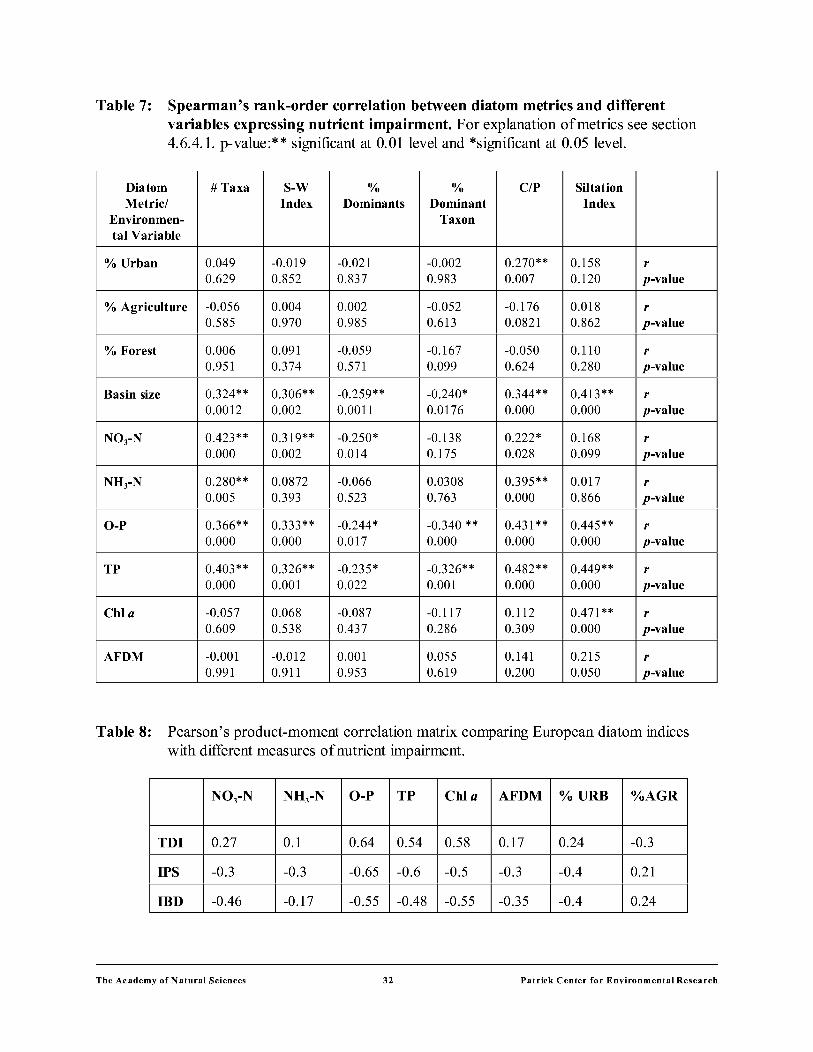
Table 7: Spearman's rank-order correlation between diatom metrics and different variables expressing nutrient impairment. For explanation ofmetrics see section 4.6.4.1. p-value:** significant at 0.01 level and *significant at 0.05 level.

Diatom #Taxa S-W 0/o 0/o C/P Siltation Metric/ Index Dominants Dominant Index

Environmen- Taxon tal Variable

%Urban 0.049 -0.019 -0.021 -0.002 0.270** 0.158 r 0.629 0.852 0.837 0.983 0.007 0.120 p-value

% Agriculture -0.056 0.004 0.002 -0.052 -0.176 O.ol8 r 0.585 0.970 0.985 0.613 0.0821 0.862 p-value

%Forest 0.006 0.091 -0.059 -0.167 -0.050 0.110 r 0.951 0.374 0.571 0.099 0.624 0.280 p-value

Basin size 0.324** 0.306** -0.259** -0.240* 0.344** 0.413** r 0.0012 0.002 0.0011 0.0176 0.000 0.000 p-value

N03-N 0.423** 0.319** -0.250* -0.138 0.222* 0.168 r 0.000 0.002 0.014 0.175 0.028 0.099 p-value

NH3-N 0.280** 0.0872 -0.066 0.0308 0.395** 0.017 r 0.005 0.393 0.523 0.763 0.000 0.866 p-value

0-P 0.366** 0.333** -0.244* -0.340 ** 0.431 ** 0.445** r 0.000 0.000 0.017 0.000 0.000 0.000 p-value

TP 0.403** 0.326** -0.235* -0.326** 0.482** 0.449** r 0.000 0.001 0.022 0.001 0.000 0.000 p-value

Chla -0.057 0.068 -0.087 -0.117 0.112 0.471 ** r 0.609 0.538 0.437 0.286 0.309 0.000 p-value

AFDM -0.001 -0.012 0.001 0.055 0.141 0.215 r 0.991 0.911 0.953 0.619 0.200 0.050 p-value

Table 8: Pearson's product-moment correlation matrix comparing European diatom indices with different measures of nutrient impairment.

I I NO,-N I NH,-N I 0-P I TP I Chi a IAFDM I %URB

I %AGR

I TDI 1 0.27 1 0.1 1 0.64 1 0.54 1 0.58 1 0.17 1 0.24 1-0.3 I IPS 1-0.3 1-0.3 1-0.65 1-0.6 1-0.5 1-0.3 1-0.4 1 0.21 I IBD 1-0.46 1-0.17 1-0.55 1-0.48 1-0.55 1-0.35 1-0.4 1 0.24


Orthophoshate versus IPS

22

20 r = -0.65 I • r 2= 0.42

18 I

• 16

• • • • • en • a.. 14 I • • 12 • •

• I • • 10 • •• • • • • • • 8 •

• • 6

0.5 1.0 1.5 2.0 2.5 3.0

log 0-P {microg/L)

Figure 11: Scatterplot of measured 0-P versus the indices calculated by Specific Polluosensitivity index (IPS) for all 2000 and 2001 samples.

In summary, the three European diatom indices were good predictors of orthophosphate and total phosphorus. Nevertheless, these results should be interpreted with caution due to differences between the European diatom flora used for the development of the indices and the diatom flora in NJ. Overall the results show that there is potential for expanding the existing European diatom models by including data for North American species.


LEGEND

WATER QUALITY

IBD

• VERY GOOD .6.

• GOOD .6.

• FAIR 6 POOR

Figure 12: Map showing the difference in the ratings of river quality as calculated by two European diatom indices, the Specific Polluosensitivity index (IPS) and the Biological Diatom Index (ffiD). The numbers correspond to NJ site ID's (see Tables 1 and 2).


6 Discussion

A main goal of this study was to explore the relationships among algal biomass, algal species composition and nutrients. A further goal was to identifY the most promising indicators for assessing excess nutrients in NJ rivers and streams using biomass and algal species composition (soft algae and diatoms). In the following paragraphs we summarize nutrient-algal relationships identified from this study and discuss the outcome of all different methods used. Finally, we discuss applicability of the indicators developed and provide recommendations towards their use and further development.

6.1 Principal factors influencing algal biomass

6.1.1 Principal variables influencing algal biomass A multitude of recent studies have been conducted to understand which combination of

factors determines algal biomass. A large amount of literature is available on this subject and a comprehensive review is published in a report presented by the New England Interstate Water Pollution Control Commission (ENSR 2001). The main factors influencing biomass accrual are nutrients, light, temperature, substrate availability and stream velocity (Biggs 1996). To determine the principal variables influencing algal biomass in our study, we analyzed all variables measured in the field and in the lab using forward stepwise regression. All factors mentioned above were included in this analysis, except for temperature measurements. To include temperature measurements we would need a long-termrecord of average daily temperatures for weeks before each sampling date. No such detailed record was available for most sites sampled. The results of a stepwise regression showed that the dependent variables Chl a and AFDM can both be predicted from a linear combination of the independent variables N03- N and river basin size. In the case of Chl a only, bigger substrate size (sum of percent bedrock, boulder, cobble and gravel) also has a significant influence on algal biomass. These results show that algal biomass in the NJ dataset is influenced by a combination of light conditions (reflected through basin size) nitrogen (N03-N) and factors closely associated with these. In our dataset TP and 0-P are strongly correlated with N03-N, therefore correlation ofChl a with N03-N also reflects correlation with phosphorus. Also, in the case of Chl a , the size of the type of substrate, and the availability of algae to attach is an additional important factor. In summary, we can deduce from this analysis that in the NJ Piedmont rivers a combination of three factors together- high light levels, high nutrient concentration, and high proportion oflarger-sized substrate - lead to the greatest quantities of algal biomass in NJ Piedmont rivers. These results suggest that there is potential for development of a metric for biomass combining all of these factors. We will explore the possibility of developing such a metric further, especially in combination with the third year data of this study.

6.1.2 Nutrient-biomass relationships as assessed by correlations After determining the main factors influencing algal biomass, we investigated the strength

ofthe relationship of individual nutrients on different measures ofbiomass. Spearman's correlation analyses showed that there is no significant and strong relationship between measured biomass concentrations ofChl a, AFDM or estimate ofbiomass as assessed through the RBA with the nutrients TP, 0-P, N03-N and NH3-N. Only the correlation betweenAFDM and nitrate


(N03-N) shows a significant trend, but the correlation is weak r = 0.26). As shown in section 6.1.1, biomass can only be explained through a combination of factors including nutrients. There is need for more detailed analysis of this dataset including the larger dataset with year 3 samples to explore the strength of the relationship between biomass and nutrients. A recent study on large datasets (national and international) on temperate streams revealed that a significant portion of variance in annual mean and maximum biomass can be explained by total nitrogen and total phosphorus concentrations (Dodds et al. 2002). The same study also shows that such relationships are very weak at the regional scale. Our study is consistent with this observation, and demonstrates the challenges offmding clear relationships at smaller (regional) scales, such as the NJ Piedmont. It demonstrates that a strong correlation between nutrient and biomass is at best difficult to establish, and that other factors such as light (as a function of river basin size) and substrate must be taken into account when estimating nutrient-biomass relationships (see section6.1.1). Therefore, commonly used biomass measures (Chl a, AFDM) must be interpreted with caution, and inferences of nutrient levels in rivers based on these measures should be made only in conjunction with analyzing other variables.

6.2 Comparison and evaluation of methods for estimating algal biomass

Algal biomass was measured in three different ways: a) we measured the contents of Chl a and AFDM contained in the composite biomass samples collected in the field; b) we estimated the proportion of cells making up most of the biomass in the composite biomass samples, using a specially designed semi-quantitative analysis and fmally c) we visually estimated proportions of abundance and thickness of algal cover in the rivers as assessed through the Rapid Bioassessment (RBA). Spearman's rank-order correlation between the different measures of biomass shows significant correlations between Chl a and with RBA estimates of biomass, with the strongest correlation between Chl a and Cladophora sp.( r = 40). In contrast, both the measures of AFDM and the estimates ofbiomass through the semi-quantitative analysis do not show significant and strong correlations with any other measures ofbiomass. Therefore, we do not recommend the use of the semi-quantitative analysis method for estimating biomass. Also, when given the choice between measuring either Chl a or AFDM as a variable to be used for biomass-algal group relationships, Chl a should be given priority.

Our study shows that a combination of measuring Chl a from composite diatom samples and using the RBA method seems to assess the amount of algal biomass best. When using those two approaches in combination, a good assessment of the biomass impairment in rivers of the NJ Piedmont can be achieved. Cladophora sp. is, based on our results, the species that correlates most closely with Chl a and is therefore the algal group that needs to be monitored most. The assessment through the RBA in combination with measuring Chl a from composite biomass samples provides a good tool for monitoring growth of Cladophora sp. Nevertheless, none of the correlations found between the different measures of biomass is very strong and therefore a combination of different methods should be used to assess biomass.


6.3 Comparison and evaluation of diatom metrics and models

In the following sections we compare the results ofthe diatommetrics and models with the objective of determining the best method for estimating phosphorus concentrations and overall water quality in NJ Piedmont rivers. The relative advantages and disadvantages of each method are discussed. Performance of all are potentially limited by how well the environmental measurements, especially nutrient concentrations, represent the variability of conditions to which the algae are exposed. It would be useful for evaluating metric effectiveness if the variability of these conditions could be quantified.

6.3.1 Nutrient-inference models The diatom species composition found in the NJ Piedmont dataset was strongly influenced

by the measured nutrient variables (0-P, TP, N03-N and NH4-N). Therefore, development of W A - inference models for nutrients was possible. We developed 4 different nutrient inference models based on the full (n=85) and a reduced dataset (n= 54). All models have relatively high predictive power. The best models developed are the TP and the N03-N inference models for the full (n=85) and a reduced dataset (n= 54). For both variables, the model developed with the full dataset (n=85) has a higher r, but the model based on the reduced dataset (n= 54) has a lower RMSEP (boot)' respectively. This means that the errors obtained for the values inferred using the TP and N03-N models developed for the full dataset will be higher than those based on the reduced dataset. Nevertheless, when we tested observed versus predicted TP for the full dataset inference model (n=85), we found that the model has relatively high predictive power r 2

(boot) = 0.55. Also, testing of the same model on the year 2 samples produced reliable results ( r 2 = 0. 61). In the future, different techniques will be applied to improve the model to increase its predictive power. Also, we plan on including samples taken during the second (2001) and the third year (2002) of this project to increase the predictive power of these two WA-inference models for N03-N and TP.

In summary, in contrast to soft algal species composition, we found good correlation between diatom assemblage composition and nutrients. The WA nutrient-inference models developed showed reliable results when tested, and we intend to improve them further. The diatom inference models seem to be better indicators for nutrients and river eutrophication than biomass. In general, species composition based indicators correlate better with nutrient concentrations, because the ecological information from diatoms is not as variable as biomass (e. g., Chl a) concentrations over time. The application of diatom inference models to N J Piedmont rivers and streams is highly recommended as a tool for monitoring eutrophication. Nutrient inference models are relatively easy to apply as a regular monitoring tool. Nevertheless, their use requires appropriate software and expertise.

6.3.2 Simple metrics The usefulness of the of the six diversity and simple metrics was evaluated by comparing

their correlations with nutrient impairment measures. Siltation Index, the Centrics/Pennates and number of taxa index, showed moderate, but significant correlations with N03-N, 0-P and TP. Therefore, it is possible to use these diatom indicators to monitor river impairment, especially of


the nutrients N03-N, 0-P and TP. The formulas for the indices are simple and calculation is easy. They could be included in the list ofmetrics in the EDAS database and analysis system used by the NJ DEP. Nevertheless the correlations obtained between the indices and the nutrient variables are not very strong and the significance of the results is questionable. We consider the results obtained through the nutrient inference models by far more reliable and recommend using simple metrics only as complementary method.

6.3.3 European indices The three European diatom indices (TDI, IBD, IPS) showed good results and relatively

strong correlation with orthophosphate and total phosphorus in the NJ Piedmont dataset. It is interesting to note that the strength of the correlation of the Northern Piedmont Diatom TP index and the British Trophic Diatom Index with Orthophosphate is similar r = 0.66 and r = 0.64 respectively). Nevertheless, we do not recommend using the European indices solely, because of important differences between the European diatom flora used for the development of the indices and the diatom flora in the NJ Piedmont.

6.4 Comparison of diatom inferred TP and impairment classifications based on macroinvertebrate metrics (AMNET)

We compared TP calculated using the diatom TP diatom inference model (n=85) to macroinvertebrate impairment ratings based on the 1998/99 assessment. The results (Fig. 13) show that the diatom inferred TP values do not correspond strongly to the macroinvertebrate impairment groups of "non-impaired," "moderately impaired" and " severely impaired." No significant separation is found between ratings, as all groups' lOth and 90th percentiles overlap to a high degree with the adjacent category. The"moderately impaired" category in particular includes a large number of sites that are indicated by the diatoms to have a wide range of TP values. Nevertheless, the sites rated "non-impaired" and "severely impaired" do show a trend ofhaving lower and higher diatom inferred TP, respectively. More detailed analysis comparing diatom inferred nutrient concentrations with macroinvertebrate metrics that best reflect nutrient (e.g., % EPT etc.) will be performed in collaboration with the NJ Integrated Assessment (Horwitz and Flinders 2003) including Year 3 data of this study.

6.5 Evaluation of the EPA percentile method for determining reference conditions

We applied the proposed U.S. EPA percentile method (U.S. EPA 2000b) to the NJ Northern Piedmont dataset to calculate reference conditions. In our study, the 25th percentile was calculated using all nutrient data from all reaches (Appendix 1 b). We compared our value to those for the aggregate of all Level III Subecoregions ofNutrient Ecoregion IX, and to the Northern Piedmont subecoregion (64) only, as given in the Ambient Water Quality Criteria Recommendations (U.S. EPA 2000b). The range ofTP reference conditions given for all subecoregions is 22.5-100 J..Lg/1; for the Northern Piedmont subecoregion it is 40 ).lg/L. We calculated a reference condition of 51 ).lg/L for the NJ Northern Piedmont, which is only 10 ).lg/L greater than the one proposed in the EPA document. The range of EPA total nitrogen reference conditions is 0.07-1.00 mg/L; it is 1.30 for the Northern Piedmont. Our dataset shows a


C> 0 C>

350 N -~ 300 C') ::::&.

250 -Q. .... 200 '"0 G> 150 t:: .! 100 c:

E 50

0 0 t;S ·-c

0

•

•

_l_ •

1 2 3

AMNET ratings 1998

n- lmpaired odent ly imp "re d

Severely impaired

4

Figure 13: Box-plots comparing diatom inferred TP to AMNET macroinvertebrate impairment ratings. Upper limit of error bars indicate the 1Oth and the 90th percentile. Filled circles indicate outliers.

25th percentile of total nitrogen of 1.28 mg/L, which is relatively near EPA's value for the Northern Piedmont. Also, the periphyton chlorophyll a measured in our dataset shows a 25th percentile of 48.07 mg/m2 which substantially exceeds the range given by EPA of 3.13-20.35 mg/m2 and the value for the Northern Piedmont of20.35. This comparison shows that, using the percentile method, there is reasonable good agreement between TP and TN reference values derived from data in the EPA study and this study, but that there is a substantial difference for Chl a values.


7 Conclusion: Recommendation for use of the ideal algal indicator monitoring program for the NJ Piedmont

Based on our study, we recommend the use of a combination of algal indicators and metrics for monitoring nutrients and biomass. For monitoring biomass, we recommend using the EPA Rapid bioassessment Protocol in combination with measuring chlorophyll a. Our results show that chlorophyll a correlates especially well with Cladophora sp. cover and that measuring both of these variables provides a good monitoring tool. Biomass can be explained by a combination of factors, such as nutrients and light conditions and there is potential for developing a biomass metric that incorporates these factors. More detailed analysis of our dataset is needed to develop such a metric, especially in combination with the third year data of this study.

Diatom assemblage composition is strongly influenced by nutrients, especially phosphorus (0-P and TP), we were therefore able to develop phosphorus inference models and indices. Inferred values and metrics were tested by comparing them with measured phosphorus values. The best results were achieved with the TP diatom inference models developed for the NJ Piedmont. We compared the results obtained for the European indices, the Biological Diatom Index, the Polluosensitivity Index and the Trophic Diatom index. All three indices showed relatively good correlations with either 0-P and/or TP, suggesting that all three methods could potentially be applied and the results compared, when using diatoms as indicators of river phosphorus in the NJ Piedmont. The biggest limitation to further development of models and metrics is probably the representativeness of nutrient values that are based on very few samples per site. Increasing the number of samples per site is recommended for future studies.

In summary, this study shows that algae can be used as indicators of nutrient impairment for the NJ Piedmont. Diatoms especially show good response to nutrients and their use as monitoring tool is highly recommended. Biomass metrics need further analysis, the possibility of developing metrics combining different factors influencing algal growth, especially nutrients is promiSmg.


References

American Public Health Association, American Water Works Association and Water Pollution Control Federation (APHA, A WW A and WPCF) 1992. Standard Methods for the Examination of Water and Wastewater, 19th ed. Washington, DC.

Bahls, L. L. 1993. Periphyton bioassessment methods for Montana streams. Montana Water Quality Bureau, Department ofHealth and Environmental Science, Helena, MT.

Barbour, M. T., J. Gerritsen, B. D. Snyder, and J. B. Stribling. 1999. Rapid bioassessment protocols for use in streams and wadeable rivers: Periphyton, benthic macro invertebrates, and fish, Second Edition. EPA 841-B-99-002, Washington, D.C., U.S. Environmental Protection Agency, Office ofWater.

Biggs, B. J. F. 1996. Patterns in benthic algae of streams. In Algal Ecology, Freshwater Benthic Ecosystems. R. J. Stevenson, M. L. Bothwell, and R. L. Lowe (eds.). Academic Press, NY.

Biggs, B. J. F. 2000. Eutrophication of streams and rivers: Dissolved nutrient-chlorophyll relationships for benthic algae. Journal ofNorth American Benthological Society 19: 17-31.

Birks, H. J. B., S. Juggins, and J. M. Line. 1990a. Lake surface-water chemistryreconstruction from paleolimnological data. In: The Surface Water Acidification Programme. Edited by B.J. Mason. Cambridge Press, Cambridge. Pp.: 301-311.

Birks, H. J. B., J. M. Line, S. Juggins, A C. Stevenson, and C. J. F. ter Braak. 1990b. Diatoms and pH reconstructions. Philosophical Transactions of the Royal Society ofLondon, series B 327: 263-278.

Birks, H. J. B. 2001. Maximum likelihood calibration and the compute program WACALIB a correction. Journal of Paleolimnology 25(1): 111-115.

Blum, J. L. 1956. The ecology ofriver algae. Botanical Review 22: 291-331.

Charles, D., D. Winter, and M. Hoffman. 2000. Field Sampling procedures for the New Jersey Algae Indicators project. PCER Procedure P-13-64. Patrick Center for Environmental Research, Academy ofNatural Sciences, Philadelphia, PA. 18 pp.

Charles, D. F., C. Knowles, R. Davis ( eds.). 2002. Protocols for the analysis of algal samples collected as part ofthe U.S. Geological Survey, National Water-Quality Assessment Program. Report No. 02-06. The Academy ofNatural Sciences. Patrick Center for Environmental Research, Academy ofNatural Sciences, Philadelphia, PA. 124 pp.


Cemagref. 1982. Etude des methodes biologiques quantitatives d'appreciation de la qualite des eaux. Rapport Division Qualite des eaux Lyon- Agence fmanciere de Bassin RhoneMediterranee- Corse, Pierre-Benite, 28 pp.

Cotter, P. 1999-2000. Tabulator, version 3.7.0. Patrick Center for Environmental Research, ANSP, Philadelphia, P A

Cotter, P. 2001. Tabulator Installation and Users Guide. Patrick Center for Environmental Research, ANSP, Philadelphia, P A. 24 pp.

Cuffuey, T. F., Gurtz, M .. E., andM. R. Meador. 1993. Methods for collecting benthic invertebrate samples as part of the National Water-Quality Assessment Program. Open-File Report 93-406. U.S. Geological Survey, Raleigh, NC. 66 pp.

Dixit, S. S., Smol, J.P., Kingston, J. C., and D. F. Charles. 1992. Diatoms: Powerful indicators of environmental change. Environmental Science and Technology 26 (1 ): 23-33.

Dodds, W. K, V. H. Smith, and K Lohman. 2002. Nitrogen and phosphorus relationships to benthic algal biomass in temperate streams. Canadian Journal of Fisheries and Aquatic Sciences 59: 865-874.

Dodds, W. K, and E. B. Welch. 2000. Establishing nutrient criteria in streams. Journal of the North American Benthological Society 19: 186-196.

Dytham, C. 1999. Choosing and Using Statistics. A Biologist's Guide. Blackwell. Oxford.

Ennis, G. L., and L. J. Albright. 1982. Distribution and abundance ofperiphyton and phytoplankton species in two Subarctic Canadian rivers. Canadian Journal of Botany 60:224-236.

Environmental and Energy Development Solutions (ENSR). 2001. The Relationships Between Nutrient Concentrations and Periphyton Levels in Rivers and Streams- A Review of Scientific Literature. New England Interstate Water Pollution Control Commission. Document Number 4933-001-400.

Fallu, M.A., N. Allaire, and R. Pienitz. 2000. Freshwater diatoms from northern Quebec and Labrador (Canada). Bibliotheca Diatomologica, Band 45: 1-200.

Fitzpatrick, F. A., Waite, I. R., D'Arconte, P. J., Meador, M. R., Maupin, M.A., and Gurtz, M. E. 1998. Revised Methods for Characterizing Stream Habitat in the National Water-Quality Assessment Program: U.S. Geological Survey Water-Resources Investigations Report 98-4052. 67 pp.

Francoeur, S.N. 2001. Meta-analysis oflotic nutrient amendment experiments: Detecting and quantifYing subtle responses. Journal of North American Benthological Society 20(3): 358-368.


Hall, R. L., and J. P. Smol. 1992. A weighted averaging regression and calibration model for inferring total phosphorous concentration from diatoms in British Columbia (Canada) lakes. Freshwater Biology27: 417-434.

Horwitz, R. and C. Flinders. 2003. Bioassessment Integration Study: Systems Ecology Evaluation ofUS EPA Rapid Bioassessment Protocols in New Jersey (Macroinvertebrates, Periphyton, Fish and Habitat) Quality ControVQuality Assurance Project Plan.

Jongman, R. H. G., C. J. F. ter Braak, andO. F. R. van Tongeren.1995. DataAnalysis in Community and Landscape Ecology. Cambridge University Press, Cambridge.

Juggins, S., and C. J. F. ter Braak. 1997. CALIBRATE- a computer program for speciesenvironmental calibration by Weighted averaging Partial least square regression. 0 .81. University ofNewcastle. Newcastle, UK.

Juggins, S., and C. J. F. ter Braak. 2001. CALIBRATE Version 1.0. A C++ Program for analysing and visualising species environment relationships and for predicting environmental values from species assemblages. User Guide Version 1.0. Department of Geography. University ofNewcastle. Newcastle, UK.

Kelly, M.G. 1998. Use of the trophic diatom index for monitoring eutrophication in rivers. Water Resources 32: 236-242.

Kelly, M. G., and B. A. Whitton, 1995. The trophic diatom index. A new index for monitoring eutrophication in rivers. Journal of Applied Phycology: 7: 433-444.

Kelly, M. G., and B. A. Whitton. 1998. Biological monitoring of eutrophication in rivers. Hydrobiologia 384: 55-67.

Kiry, P., D. Velinsky, and A.-M. Compton. 1999. Determination of dry weight and percent organic matter for sediments, tissues and benthic algae. PCER Procedure P-16-113. Patrick Center for Environmental Research, Academy ofNatural Sciences, Philadelphia, PA. 3 pp.

Lecointe, C., M. Coste. and J. Prygiel. 1993. OMNIDIA: A software for taxonomy, calculation of diatom indices and inventories management. Hydrobiologia 269/270: 590-513.

Line, J. M., C. J. F. ter Braak, and H. J. B. Birks. 1994. WACALIB version 3.3- a computer program to reconstruct environmental variables from fossil assemblages by weighted averaging and to derive sample-specific errors of prediction. Journal of Paleolimnology 10: 147-152.

New Jersey Department of Environmental Protection (NJ DEP). 1999. Geologic Map ofNew Jersey. NJ DEP, Division of Science and Research, Geological Survey.


New Jersey State Department of Environmental Protection (NJ DEP). 1994. The establishment of ecoregion biological reference sites for New Jersey streams. Incorporating Habitat Quality and Benthic Macroinvertebrate Communities 1989 - 1993 Monitoring Data. State ofNew Jersey, Christine Todd Whitman Governor, Robert C. Shinn, Jr. Commissioner. Trenton, NJ.

New Jersey Department of Environmental Protection. (NJ DEP). 2000. Water Quality Monitoring Networks 2000. NJ DEP Division of Watershed Management. Trenton, NJ.

New Jersey Department of Environmental Protection (NJ DEP). 2001. Surface water quality standards. N.J.A.C. 7:9B. Trenton, NJ. 129 pp.

Moulton, S. R., J. G. Kennen, R. M. Goldstein, and J. A. Hambrook. 2002. Revised Protocols for Sampling Algal, Invertebrate and Fish Communities as Part of the National Water-Quality Assessment Program. Open-File Report 02-150. US Geological Survey, Reston, VA. 75 pp.

Omernik, J. M. 1987. Ecoregions of the conterminous United States. Annals ofthe Association of American Geographers. 77(1):118-125.

Office ofthe New Jersey State Climatologist (ONJSC). 1994-2002. Rutgers University.

Patrick Center for Environmental Research. 2000. Quality Assurance Project Plan, Project Name: Understanding the Relationship Between Natural Conditions And Loadings on Eutrophication: Algal Indicators ofEutrophication for New Jersey Streams, The Academy of Natural Sciences, Philadelphia, P A.

Patrick, R. 1951. A proposed biological measure of stream conditions. Verhandlungen. Internationale Vereinigung fur Theoretische und Angewandte Limnologie 11: 299-307.

Ponader, K., and D. Winter. 2002. Procedure for semi-quantitative analysis of soft-algae and diatoms. Patrick Center for Environmental Research. Procedure No. P-13-65. Patrick Center for Environmental Research, The Academy ofNatural Sciences, Philadelphia, PA. 6 pp.

Porter, S.D., T. F. Cuffuey, M. E. Gurtz, and M. R. Meador. 1993. Methods for Collecting Algal Samples as Part of the National Water-Quality Assessment Program. Open-File Report 93-409. U.S. Geological Survey, Raleigh, NC. 39 pp.

Prygiel J. and M. Coste. 1999. Progress in the use of diatoms for monitoring rivers in France. In: J. Prygiel, B. A Whitton. and J. Bukowska ( eds.), Use of Algae for Monitoring Rivers III. Agence de l'eau Artois-Picardie, Douai, (France). pp. 165-179.

Reed, T. J., B. T. White, G. L. Centinaro, J. F. Dudek, V. Corcino, A. B Spehar, and A. R. Protz. 2002. Water Resources Data, New Jersey, Water Year 2001. Volume 1. Surface-Water Data. Water-Data Report, NJ-01-1. West Trenton, NJ. 297 pp.


Schwoerbel, J. 1999. Einfiihrung in die Limnologie. Gustav Fischer Verlag. Stuttgart.

Smith, V. H., Tilman, G. D., and J. C. Nekola. 1999. Eutrophication: Effects of excess nutrient inputs on freshwater, marine, and terrestrial ecosystems. Environmental Pollution 100: 179-196.

Stevenson, R. J. andY. Pan. 1999. Assessing environmental conditions in rivers and streams with diatoms. In: Stoermer E. F. and J. P. Smol (eds.). The Diatoms: Applications for the Environmental and Earth Sciences. Cambridge University Press, Cambridge, UK. Pp.11-40.

Tedrow, J. C. F. 1986. Soils ofNew Jersey. Robert E. Krieger Publishing Company, Inc., Malabar, FL.

ter Braak, C. J. F. and I. C. Prentice, 1998. A theory of gradient analysis. Advances in Ecological Research 18:221-317.

ter Braak, C. J. F. and H. Van Dam. 1989. Inferring pH from diatoms: A comparison of old and new calibration methods. Hydrobiologia 178: 209-223.

U.S. EPA. 1992. Methods for the determination of chemical substances in marine and estuarine environmental samples. EPA/600/R-92/121, Office ofResearch and Development, U.S. EPA, Washington, D.C.

US. EPA. 2000a. Nutrient Criteria Technical Guidance Manual: Rivers and Streams, U.S. Environmental Protection Agency, Washington, DC. EPA-822-B-00-002.

US. EPA. 2000b. Ambient Water Quality Criteria Recommendations: Rivers and Streams in Nutrient Ecoregion IX. U.S. Environmental Protection Agency, Washington, DC. EPA-822-B-00-019.

Velinsky, D. 2000. Syringe water sampling and filtration for the collection of filtered nutrient samples and unfiltered nutrient samples. PCER Procedure P-16-119. Patrick Center for Environmental Research, Academy of Natural Sciences, Philadelphia, P A. 4 pp.

Velinsky, D., and J. DeAlteris. 2000. Benthic algae and sediment chlorophyll a preparation and analysis. PCER Procedure P-16-117. Patrick Center for Environmental Research, Academy of Natural Sciences, Philadelphia, PA. 4 pp.

Winter, J. G. and H. C. Duthie. 2000. Epilithic diatoms as indicators of stream total N and total P concentration. Journal of the North American Benthological Society 19(1): 32-49.

Wolfe, P. E. 1977. The Geology and Landscapes ofN ew Jersey. Crane, Russak and Company, Inc., N.Y. 351 pp.


Appendix 1 Summary of site characteristics. All sites sampled in 2000 and 2001.

la) Raw environmental data for variables measured at each site reach.

Note: All variables were measured by PCER staff in the field at time of algal sampling and/or in the laboratory. General site characteristics: Sr_no, site reach number; S_date, algae sampling date; B_size, basin size; %0, percent open canopy cover; R _len, reach length; R _wid, average river width at reach; Flow, flow estimate in categories (1 =slow; 2=moderate; 3=fast); Substrate: %Bed, %bedrock; %Bo, %boulder; %Cob, % cobble; %Gra, % gravel; %S, % sand; %Si/Cl, % silt and clay. Biomass: AFDM, Ash free dry mass; Chl_ a, chlorophyll a;

SitelD

IIAN0081

IIAN0081

IIAN0081

llANO! II

llANO! II

IIANOII5

IIANOII5

IIANOII5

IIANOII5

IIANOII5

IIANOII5

IIAN0118

IIAN0118

IIAN0118

IIAN0192

IIAN0192

IIAN0192

IIAN0194

IIAN0194

IIAN0194

IIANOI95

IIANOI95

IIANOI95

IIAN0207

IIAN0207

IIAN0207

IIAN0209

IIAN0209

IIAN0209

IIAN0211

IIAN0211

IIAN0211

IIAN0211

IIAN0211

IIAN0211

IIAN0215

IIAN0215

IIAN0215

IIAN0227

IIAN0227

IIAN0227

IIAN0231

IIAN0234

IIAN0234

Sr_no S_date

NJ_081 10:22 am

NJ_081_2 10:22 am

NJ_081_3 10:22 am

NJ_lll_l 10:22 am

NJ_lll_2 10:22 am

NJ_ll5_1 10:22 am

NJ_ll5_2 10:22 am

NJ_ll5_3 10:22 am

NJ_ll5_1 10:22 am

NJ_ll5_2 10:22 am

NJ_ll5_3 10:22 am

NJ_ll8_1 !0:22am

NJ_ll8_2 !0:22am

NJ_ll8_3 !0:22am

NJ_l92_1 10:22 am

NJ_l92_2 10:22 am

NJ_l92_3 10:22 am

NJ_l94_1 10:22 am

NJ_l94_2 10:22 am

NJ_l94_3 10:22 am

NJ_l95_1 10:22 am

NJ_l95_2 10:22 am

NJ_l95_3 10:22 am

NJ_207 _I 10:22 am

NJ_207 _2 10:22 am

NJ_207 _3 10:22 am

NJ_209_1 10:22 am

NJ_209_2 10:22 am

NJ_209_3 10:22 am

NJ_211_1 !0:22am

NJ_211_2 !0:22am

NJ_211_3 !0:22am

NJ_211_1 !0:22am

NJ_211_2 !0:22am

NJ_211_3 !0:22am

NJ_215_1 10:22 am

NJ_215_2 10:22 am

NJ_215_3 10:22 am

NJ_227_1 10:22 am

NJ_227_2 10:22 am

NJ_227_3 10:22 am

NJ_231_1 10:22 am

NJ_234_1 10:22 am

NJ_234_2 10:22 am

Tbe Academy of Nat ural Sciences

% 0 %Bed %Bo %Cob %Gra %San %Si/Cl

100 0 16.7 35 38.3 10 0

62.4 20 15 35 31.7 11.7 0

12.48 23.3 10 18.3 20 8.3 0

16.64 0 20 45 30 0

6.24 0 30 15 30 20

23.92 0 0 15 80 0

31 .2 0 0 2 25 73 0

26 0 0 0 15 85 0

9.375 0 0 15 80 0

11.46 0 0 2 25 73 0

19.79 0 0 0 15 85 0

82.16 0 50.8 20.8 25.8 4.2 0

86.32 0 21.7 39.2 38.3 0.8 0

22.88 0 35 60 0 0

14.58 0 40 30 20 10 0

18.75 0 10 20 30 30 10

53.13 0 20 70 0

82.16 0 0 0 0 50 50

100 0 0 0 0 50 50

100 0 0 0 0 50 50

21.84 0 0 35 55 10 0

26 0 0 45 45 10 0

76.96 0 0 35 60 0

69.79 0 0 0 90

55.21 0 15 25 40 20 0

28.13 0 20 40 30 10 0

1.042 0 0 30 30 40 0

50 0 15 30 20 40

7.292 0 10 50 10 30 0

5.2 0 I 0 40 20 30 0

17.16 0 10 20 10 60 0

14.56 0 30 25 40 0

9.375 0 10 40 20 30 0

15.63 0 10 20 10 60 0

16.67 0 30 25 40 0

53.04 0 25 20 45

3.12 0 30 20 40

5.2 0 15 70

75.92 0 0 0 0 50 50

58.76 0 0 0 0 50 50

78.52 0 0 0 0 50 50

100 0 0 0 0 50 50

11.44 0 45 45 0

10.4 0 15 40 30 15 0

46

7

7

4

4

4

4

4

4

20

20

20

2. 75

2. 75

2. 75

6

6

6

11.5

11.5

11.5

15

15

15

3.5

3.5

3.5

7

7

7

50

9

9

50

50

50

15

30

25

25

30

25

25

50

50

50

20

20

20

30

30

30

40

40

40

50

50

50

30

30

30

20

20

20

20

20

20

16.5

16.5

16.5

25

25

25

50

40

40

2

2

2

1.5

2

2

2

1.5

2

1.5

2.5

2

1.5

2

2

2.5

1.5

2

2

1.5

2

1.5

1.5

1.5

1.5

2

2

2.5

2.5

16.3

8.9

4.8

17 .I

12.6

78.9

10.8

32 .I

22.7

24.8

20.1

15 3.1

11.8

7.6

8.8

5.4

8.1

23.2

33 .I

22.8

4.2

9.5

8.5

16.1

11.5

12.5

18.7

21.9

16.9

17.5

11.9

14.4

5.6

3.8

5.0

30.2

17.9

8.1

15 2.81

83.31

37.41

73 .41

64.21

98.41

30.91

32.81

69.71

85 .1l 111.51

lll4.71 64.51

14.41

41.41

17.21

69.91

--I --I --I

12 8.81

22 8.51

15 2.31

36.71

40.41

48.91

86.01

70.61

62.71

67.61

75 .ol 80.91

52.31

43 .1l 75.81

32.61

2.21

5.51

--I --I --I

29.21

179.31

47.81

Patrick Center for EnvironmentalResearcb

SitelD Sr_no S_date % 0 %Bed %Bo %Cob %Gra %San %Si/Cl

IIAN0234 NJ_234 10:22 am 21.84

IIAN0234 NJ_234_1 10:22 am 89.58

IIAN0234 NJ_234_2 10:22 am 7.292

IIAN0234 NJ_234_3 10:22 am 100

IIAN0235 NJ_235_1 10:22 am 59.38

IIAN0235 NJ_235_2 10:22 am 48.96

IIAN0235 NJ_235_3 10:22 am 39.58

IIAN0237 NJ_237_1 10:22 am 2.083

IIAN0237 NJ_237_2 10:22 am 7.292

IIAN0237 NJ_237_3 10:22 am 30.21

IIAN0238 NJ 238 I 10:22 am 46.8

IIAN0238 NJ 238 2 10:22 am 6.24

IIAN0238 NJ 238 3 10:22 am 14.56

IIAN0267 NJ_267 _I 10:22 am 80.08

IIAN0267 NJ_267_2 10:22 am 88.4

IIAN0267 NJ_267_3 10:22 am 82.16

IIAN0274 NJ_274_1 10:22 am 100

IIAN0274 NJ 274 I 10:22 am 64.48

IIAN0281 NJ_281_1 10:22 am 5.2

IIAN0281 NJ_281_2 10:22 am 13.52

IIAN0281 NJ_281_3 10:22 am 79.04

IIAN0291 NJ_291_1 10:22 am 64.89

IIAN0291 NJ_291_2 10:22 am 78

IIAN0291 NJ_291_3 10:22 am 74.36

IIAN0318 NJ_318_1 10:22 am 16.64

IIAN0318 NJ_318_2 10:22 am 19.76

IIAN0318 NJ_318_3 10:22 am 38.48

IIAN0321 NJ_321_1 10:22 am 40.56

IIAN0321 NJ_321_2 10:22 am 77.48

IIAN0321 NJ_321_3 10:22 am 16.02

IIAN0326 NJ_326_1 10:22 am 92.56

IIAN0326 NJ_326_2 10:22 am 87.36

IIAN0326 NJ_326_3 10:22 am 84.24

IIAN0333 NJ_333_1 10:22 am 65.63

IIAN0333 NJ_333_2 10:22 am 65.63

IIAN0333 NJ_333_3 10:22 am 92.71

IIAN0339 NJ_339_1 10:22 am 29.12

IIAN0339 NJ_339_2 10:22 am 11.44

IIAN0339 NJ_339_3 10:22 am 29.12

IIAN0341 NJ_341_1 10:22 am 100

IIAN0341 NJ_341_2 10:22 am 100

IIAN0341 NJ_341_3 10:22 am 100

IIAN0370 NJ_370_1 10:22 am 100

IIAN0370 NJ_370_2 10:22 am 100

IIAN0370 NJ_370_3 10:22 am 100

IIAN0374 NJ_374_1 10:22 am 100

IIAN0374 NJ_374_2 10:22 am 100

IIAN0374 NJ_374_3 10:22 am 100

IIAN0374 NJ_374_1 10:22 am 86.46

IIAN0374 NJ_374_2 10:22 am 75

IIAN0374 NJ_374_3 10:22 am 87.5

IIAN03 82 NJ 3 82 I I 0:22 am 87

IIAN0382 NJ 382 2 10:22 am 100


0

0

0

0

0

0

0

0

0

0

0

0

0

0

0

0

0

0

0

0

0

0

0

0

0

0

0

0

0

0

0

0

0

0

0

0

0

0

0

0

0

0

0

0

0

0

0

0

0

0

0

0

0

15 50

45

15 40

15 50

15 30

0 25

0 10

30 30

60 30

70 20

0 0

0 0

0 0

23.3 44.2

16.7 34.2

25

30 30

33 .3 33 .3

6.7 26.7

10 16.7

25

20 40

0 3.3

1.7 15

55 16.7

40 30

21.7 28.3

13.3 38.3

6.7 41.7

2.5 35

15 35

15 35

15 35

0 20

0 30

0 30

6.7 36.7

20

0 45

1.7 58.3

0 35

8.3 26.7

0 14.2

0 44.2

0 23.3

16.7 16.7

1.7 43 .3

0 38.3

16.7 16.7

1.7 43 .3

0 38.3

0 0

0 0

47

30

45

30

30

25

35

30

20

10

10

0

0

0

17.5

30

46.7

30

33.3

35

35

41.7

35

31.7

30

10

13.3

13.3

18.3

25

25

35

35

35

65

50

50

51.7

53.3

38.3

31.7

40

30

59.2

30

51.7

36.7

35

36.7

36.7

35

36.7

0

0

15

30

40

60

20

0

0

50

50

50

15

19.2

23.3

10

0

31.7

38.3

31.7

65

53.3

18.3

16.7

36.7

30

26.7

37.5

15

15

15

10

10

10

21.7

16.7

6.7

16.7

30

26.7

25.8

25

25

18.3

25

25

18.3

25

0

0

0

0

0

0

0

0

0

0

0

0

50

50

50

0

0

0

0

0

0

0

0

0

0

0

0

0

0

0

0

0

0

0

0

10

10

0

0

0

1.7

8.3

0

0

0

1.7

0

1.7

0

100

100

9

9

9

9

20

20

20

12

12

12

34

34

34

45

45

4.5

4.5

4.5

16.5

16.5

16.5

8.5

8.5

8.5

27

27

27

II

II

II

25

25

25

20

20

20

35

35

35

35

35

35

20

20

40 2.5

40 2.5

40 2

40 2

60 2

60 2.5

60 1.5

20 1.5

30 2.5

30 2

40 1.5

40 1.5

40 1.5

125 2

I 00 1.5

120 2

12.5

12.5 2.5

25 2.5

32 2.5

32 2.5

60 2.5

50 1.5

50 2

40 2

40 2

40 1.5

40 2.5

40 2

40 2

90 2

90 2

90 2

50

50

50

25 2

25 1.5

25 2

77.5 2

77.5 2

75 2

75 2.5

65 2

65 2

100 2.5

75 2.5

75

100 2

75 2.5

75 2

25

25

9.1 87.21

12.9 82.51

9.2 42.31

9.8 52.51

22.9 183.51

13.2 97.91

9.9 101.81

5.2 43 .ol 7.5 58.81

10.0 122.11

--I --I --I

11.4 82.41

9.0 80.61

6.3 44.61

10.1 86.81

--I 9.9 24.91

4.5 29.41

18.9 202.21

73.5 592.81

45.0 262.71

44.9 522.61

7.6 53.21

10.0 63.21

8.0 69.d

12.4 93.81

13.4 109.81

6.9 36.91

25.5 200.21

20.7 178.41

18.0 134.81

26.4 28 0.61

27.9 206.21

12.7 95.71

28.9 145.01

12.0 51.31

8.7 66 .ol 9.4 60.41

19.9 140.81

15.2 112.01

30.8 117.01

71.9 288.d

20.1 129.11

7.0 15 3.31

29.3 214.21

48.1 324.81

13 .I 91.61

3.8 21.91

18 .I 115.0 I --I --I


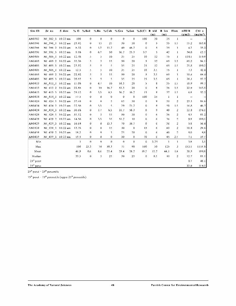
SitelD Sr_no S_date % 0 %Bed %Bo %Cob %Gra %San %Si/Cl

IIAN0382 NJ 382 10:22 am 100 0

IIAN0396 NJ_396_1 10:22 am 23.92 0

IIAN0396 NJ_396_2 10:22 am 8.32 0

IIAN0396 NJ_396_3 10:22 am 9.88 0

IIAN0405 NJ_ 405_1 10:22 am 12.48

IIAN0405 NJ_ 405_2 10:22 am 35.36

IIAN0405 NJ_ 405_3 10:22 am 23.92

IIAN0405 NJ_405_1 !0:22am 12.5

IIAN0405 NJ_ 405_2 10:22 am 22.92

IIAN0405 NJ_ 405_3 10:22 am 20.83

IIAN0413 NJ_ 413_1 10:22 am 15.08 0

IIAN0413 NJ_ 413_2 10:22 am 22.88 0

IIAN0413 NJ_ 413_3 10:22 am 29.12 0

IIAN0414 NJ 414 I 10:22 am 57.5 0

IIAN0424 NJ_ 424_1 10:22 am 37.44 0

IIAN0424 NJ_ 424_2 10:22 am 27.56 0

IIAN0424 NJ_ 424_3 10:22 am 30.68 0

IIAN0429 NJ_429_1 !0:22am 55.12 0

IIAN0429 NJ_ 429_2 10:22 am 14.56 0

IIAN0429 NJ_429_3 !0:22am 16.64 0

IIAN0439 NJ_439_1 !0:22am 13.78 0

IIAN0439 NJ_ 439_2 10:22 am 18.2 0

AN0439 NJ 439 3 10:22 am 19.5 0

M~ 0

Max 100 23.3

Mean 46 .9 0.6

Median 33 .3 0

25'h perc!

75th erct

25'h perc!= 25'h percentile

75'h perc!= 75'h percentile (upper 25'h percentile)


0

15

1.7

6.7

6.7

10

3.3

0

0

3.3

1.7

3.3

0

0

0

0

0

70

8.6

0

25

11.7

30

10

15

10

15

10

16.7

8.3

0

8.3

15

35

13.3

15

0

0

58.3

22.4

25

48

0 0

30 30

40 46.7

36.7 23 .3

35 35

50 20

35 25

35 35

50 20

35 25

58.3 20

53 .3 20

56.7 16.7

0 0

65 30

20 71.7

31.7 58.3

50 30

51.7 10

70 16.7

40 0

75 20

30 0

0 0

75 90

29.4 28.7

30 25

100

0

0

3.3

10

25

10

25

0

15

100

0

0

0

0

0

0

45

0

70

0

100

10.2

0

20

12

12

12

3.5

3.5

3.5

35

9

9

9

6

6

6

6

6

6

2. 75

50

12.7

8.5

25

35 1.5

35

42

75

65 1.5

65 1.5

75

65

65

35 1.5

36 1.5

37 1.5

50 2

50 1.5

40 2

36 2

36 2

36 2

60 2

40 2

45 2.5

125

44.1 1.8

40 2

--I 55.2 103.81

4.7 35.21

34.0 62.51

118.1 119.91

65.2 94.d

75.8 100.21

7.3 42 .ol 10.4 69.41

28 .I 87.31

10.9 99.71

22.9 143.51

6.8 52.21

--I 23 .I 84.81

16.8 46.31

22.8 136.11

8.5 sui 9.9 100.d

5.8 56.61

10.8 29.81

8.0 9.81

7.1 19.51

3.8 2.d

15 3.1 1114.81

20.5 109.81

12.1 sui 8.7 48.d

22.9 119.2


Appendix 1 Summary of site characteristics. All sites sampled in 2000 and 2001.

1 b) Raw environmental data for variables measured at each site.

Note: S_date, algae sampling date2l; Landuse: Urb %, percent urban1

l; Agr %, percent agriculture1l; For%,

percent forestry1l; Waterchemistry: Cond, specific conductivity); NH3-N

2l; N03-N2); TN, total nitrogen1

l (*TN calculated from combination ofTKN1

) and N03-N2)); TKN, total Kjeldahl nitrogen1); P04 , orthophospate2

); TP,

total phosphorus2); pH1

); Alk, alkalinity); Hard, hardness2);

t) data provided byNJ DEP and/or data records collected by NJ DEP and USGS at surface water monitoring stations, measured within a maxiumum of 4 weeks from algal sampling. 2

) variable measured by PCER Geochemistry section.

Site ID Lat Long S_date Area Urb Agr For Cond NH,-N NO,-N TN TKN

IAN0081

IANOIII

IANOII5

IANOII5

IANOII8

IANOI92

IANOI94

IANOI95

IAN0207

IAN0209

IAN0211

IAN0211

IAN0215

IAN0227

IAN0231

IAN0234

IAN0234

IAN0235

IAN0237

IAN0238

IAN0267

IAN0274

IAN0274

IAN0281

IAN0291

IAN0318

IAN0321

IAN0326

IAN0333

IAN0339

IAN0341

IAN0370

IAN0374

IAN0374

IAN0382

IAN0396

IAN0405

IAN0405

IAN0413

IAN0414

N W

40" 32' 75" 02'

40" 17' 74" 42'

40" 14' 74" 41'

40" 14' 74" 41'

40" 13' 74" 45'

40" 46' 74" 16'

40" 40' 74" 18'

40" 37' 74" 16'

40" 59' 74" 01'

40" 58' 73" 58'

40" 54' 74. 02'

40" 54' 74. 02'

40" 46' 74. 32'

40" 38' 74" 31'

40" 49' 74. 20'

40" 48' 74. 27'

40" 48' 74. 27'

40" 49' 74. 26'

40" 51' 74" 23'

40" 50' 74. 20'

41" 02' 74" 14'

40" 53' 74" 13'

40" 53' 74" 13'

41"01' 74"06'

40" 51' 74" 06'

40" 43' 74. 54'

40" 38' 74" 58'

40" 34' 74. 52

40" 28' 74. 49'

40" 33' 74" 47'

40" 32' 74" 41

40"38' 74"41'

40" 34' 74. 40'

40" 34' 74. 40'

40" 19' 74" 36'

40" 22' 74. 36'

40" 25' 74" 38'

40" 25' 74" 38'

40" 32' 74. 35'

40" 32' 74. 34'

36782

36793

36746

37128

36801

37124

36796

36787

37125

37125

36796

37126

36783

36800

37124

36795

37123

37123

37124

36800

36794

km'

24.8

15.7

27 .I

27 .I

23 3.2

10.1

78.2

104.9

42.1

22.3

15 .4

15 .4

1.4

146.6

33 9.1

72.6

72.6

82.6

27.2

17 8.9

72.2

36800 1612.2

371 26 1612.2

36788

36797

36781

36781

36782

37122

36775

36780

36775

36779

37122

36801

36774

36776

37128

36780

36800

19.6

135.4

14.4

30

386.9

65.5

10.3

685.6

25 6.3

484.2

484.2

112.6

24.2

56.3

56.3

40.6

734.3

% 16

39

46

46

43

76

75

79

80

86

92

92

6

37

48

47

47

51

61

55

29

37

37

82

82

13

24

25

24

31

25

24

28

28

22

30

28

28

48

31

% 53

30

23

23

20

0

0

0

0

0

0

0

7

4

2

0

0

19

20

21

41

30

28

23

21

21

32

14

23

23

16

25

% 21

13

10

20

20

16

II

10

93

26

23

43

43

39

23

27

60

43

43

II

10

51

43

41

22

33

33

43

42

42

16

25

31

31

17

22

144 0.006

298 0.045

93 0.066

192 0.16

292 0.126

983 0.086

0.075

407 0.033

552 0.159

453 0.177

658 0.068

214 0.116

0.008

0.023

670 0.097

209 0.068

327 0.061

434 0.012

436 0.023

0.082

303 0.027

389 0.032

478 0.022

493 0.024

595 0.14

0.002

0.004

269 0.008

275 0.012

210 0.003

269 0.026

255 0.005

251 0.006

298 0.021

0.032

212 0.012

285 0.024

529 0.016

282 0.012

0.077

1.579 1.6

I. 744

1.154 l.ll

2.565 3.315*

2.492 3·7

0.397 0.937*

1.349

0.966 1.303

2.535 3.175*

1.529 1.829*

1.102 2.008

1.128 1.688*

0.265

7.553

5.032 5.742*

1.974 0.89

1.366 1.856*

2.306

0.232

2.099

1.238 0.987

3.106 2·5

2.591

1.924

5.524 5 · 11

0.342

0.822

1.308 I. 766

1.091 1.381 *

1.104

1.275 1.9

1.046 1.5

0.516 1.421

0.652 0.982*

4.273

4.557 2 ·071

3.11

5. 73

1.344

2.546

0.5

0.8

0.75

0.7

0.54

0.428

0.64

0.3

0.323

0.56

0.71

0.7

0.49

0.286

0.8

0.66

0.804

0.326

0.29

0.5

0.4

0.457

0.33

0.536

PO, TP pH Alk

0.041 0.051

0.04 0.071

0.004 0.026

0.001 0.012

0.268 0.322

0.034 0.056

0.019 0.063

0.041 0.075

0.232 0.337

0.015 0.055

0.02 0.05

0.042 0.082

0.008 0.022

1.1 35 1.297

0.573 0.699

0.116 0.153

0.07 0.125

0.078 0.118

0 ·02 0.064

0.168 0.262

0.088 0.11

0.447 0.506

0.359 0.458

0.011 0.032

0.662 0. 73

0.006 0.011

0.015 0.034

0.022 0.042

0.01 0.035 0 ·06 0.068

0.079 0.103

0.064 0.082

0.012 0.032

0.044 0.063

0.041 0.065

0.014 0.024

0.077 0.103

0.045 0.06

0.087 0.11

0.247 0.288

7

7

7

7

7

7

8

9

7

7

20

80

90

100

48

90

55

70

95

70

78

72

80

-I -I -I

551

-I 2801

-I -I

1401

15ol

-I 651

-I -I

15ol

I 951

1151 1581

-I -I -I

1201 -I -I -I -I -I

1051

-I -I -I -I

1051

-I -I -I

1701

-I -I

Tbe Academy of Nat ural Sciences 49 Patrick Center for EnvironmentaiResearcb

SitelD Lat Long S_date Area Urb Agr For Cond NH,-N NO,-N TN TKN PO, TP pH Alk

N w km' % % % /L

IAN0424 40" 34' 74" 29' 36786 60.1 79 0 460 0.15 0.969 0.6 0.067 0.1 -I

IAN0429 40" 30' 74" 28' 36786 14.8 91 0 461 0.024 1.307 0.076 0.093

:I AN0439 40" 17' 74" 23' 36773 51.9 23 24 19 0.057 0.538 0.012 0.062

IMin 40" 13' 73. 58' 36746 1.4 6 0 93 0.002 0.232 0.89 0.286 0.001 0.011 7 20 551

IMax 41" 02' 75" 02' 37128 1612.2 92 53 93 983 0.177 7.553 5.742 0.804 1.135 1.297 9 100 2801

!Mean 199 46 13 26 373 0.052 2.007 1.941 0.537 0.127 0.166 73 ml

!Median 60.1 39 7 23 300 0.027 1.349 1.6 0.536 0.044 0.071 78 1201

l25'h perct 24.5 28 0 12 259 0.012 1.069 1.277 0.4 0.017 0.051 70 1051

175'h Eerct 162.8 68 23 41 461 0.067 2.541 2.04 0.7 0.088 0.122 90 15ol

25'h perc!= 25'h percentile

75'h perc!= 75'h percentile (upper 25'h percentile)

Tbe Academy of Nat ural Sciences 50 Patrick Center for EnvironmentalResearcb

Appendix 2: Diatom species list

Taxonomic index of 306 diatom species from samples collected in 2000 and 2001, used for development of models and metrics. Numbers correspond to numbers used in graphs in the text.

No. Taxon name

Achnanthidium minutissimum (Kiitzing) Czarnecki 2 Achnanthes exigua Grunow 3 Achnanthes lanceolata (Brebisson in Kiitzing) Grunow 4 Achnanthes lapidosa Krasske 5 Achnanthes linearis (Smith) Grunow 6 Achnanthes sp.1 NEW JERSEY KCP 7 Achnanthes peragalli Brun et Heribaud 8 Achnanthes pinnata Hustedt 9 Achnanthes lanceolata var. apiculata Patrick 10 Achnanthes delicatula (Kiitzing) Grunow 11 Achnanthes lanceolata subsp. rostrata (0estrup) Lange-Bertalot 12 Achnanthes chlidanos Hohn et HeUermann 13 Achnanthes lanceolata var. abbreviata Reimer 14 Achnanthes subhudsonis var. kraeuselii Cholnoky 15 Achnanthes minutissima var. saprophila Kobayasi et Mayama 16 Achnanthes harveyi Reimer 17 Achnanthes exigua var. constricta Torka 18 Achnanthes petersonii Hustedt 19 Achnanthes rupestoides Hohn 20 Achnanthes minutissima var. scotica (Carter) Lange-Bertalot 21 Achnanthes subatomus Hustedt 22 Achnanthes daui Foged 23 Achnanthes grana Hohn & HeUermann 24 Achnanthes lanceolata subsp. frequentissima Lange-Bertalot 25 Amphora ovalis (Kiitzing) Kiitzing 26 Amphora libyca Ehrenberg 27 Amphora montana Krasske 28 Amphora pediculus (Kiitzing) Grun. 29 Asterionella formosa Has sal 30 Aulacoseira pfaffiana (Reinsch) Krammer 31 Aulacoseira ambigua (Grunow) Simonsen 32 Aulacoseira distans (Ehrenberg) Simonsen 33 Aulacoseira subartica (0. Muller) Haworth 34 Aulacoseira granulata (Ehrenberg) Simonsen 35 Aulacoseira italica (Ehrenberg) Simonsen 36 Caloneis bacillum (Grunow) Cleve 37 Caloneis hyalina Hustedt 38 Caloneis silicula (Ehrenberg) Cleve 39 Capartogramma crucicula (Grunow ex Cleve) Ross 40 Cocconeis placentula var. lineata (Ehrenberg) Van Heurck 41 Cocconeis placentula var. euglypta (Ehrenberg) Cleve


4 2 Cocconeis fluviatilis Wall ace 43 Cocconeis pediculus Ehrenberg 44 Cyclostephanos tholiformis Stoermer, Hakansson et Theriot 45 Cyclostephanos invisitatus (Hohn et Hellermann) Theriot, Stoermer et Hakansson 46 Cyclotella atomus Hustedt 4 7 Cyclotella meneghiniana Kiitzing 48 Cyclotella ocellata Pantosek 49 Cyclotella stelligera (Cleve et Grunow) Van Heurck 50 Cyclotella pseudostelligera Hustedt 51 Cyclotella operculata (Agardh) Kiitzing 52 Cyclotella sp. 1 ANS NEW JERSEY KCP 53 Craticula cuspidata (Kiitzing) Mann 54 Cymatopleura solea (Brebisson) Smith 55 Cymbella naviculiformis Auerswald ex Heribaud 56 Cymbella aspera (Ehrenberg) Peragallo 57 Cymbella tumida (Brebisson ex Kiitzing) Van Heurck 58 Cymbella proxima Reimer 59 Cymbella tumidula Grunow ex Schmidt 60 Denticula elegans Kiitzing 61 Diatoma mesodon (Ehrenberg) Kiitzing 62 Diatoma vulgaris Bory 63 Diploneis oblongella (Naegeli ex Kiitzing) Ross 64 Diploneis puella (Schumann) Cleve 65 Epithemia turgida var. westermannii (Ehrenberg) Grunow 66 Eunotia exigua (Brebisson ex Kiitzing) Rabenhorst 67 Eunotia formica Ehrenberg 68 Eunotia pectinalis var. minor (Kiitzing) Rabenhorst 69 Eunotia praerupta Ehrenberg 70 Eunotia praerupta var. bidens (Ehrenberg) Grunow 71 Eunotia minor (Kiitzing) Grunow 72 Eunotia bilunaris (Ehrenberg) Mills 73 Fragilaria capucina Desmazieres 7 4 Fragilaria construens (Ehrenberg) Grunow 75 Fragilaria crotonensis Kitton 76 Fragilaria pinnata Ehrenberg 77 Fragilaria pinnata var. lancettula (Schumann) Hustedt 78 Fragilaria vaucheriae (Kiitzing) Petersen 79 Fragilaria brevistriata var. inflata (Pantocsek) Hustedt 80 Fragilaria fasciculata (Agardh) Lange-Bertalot 81 Fragilaria nanana Lange-Bertalot 82 Fragilaria capucina var. gracilis (Oestrup) Hustedt 83 Fragilaria capucina var. rumpens (Kiitzing) Lange-Bertalot 84 Fragilaria parasitica var. subconstricta Grunow 85 Fragilaria sp. 1 ANS NEW JERSEY KCP 86 Fragilaria sp. 1 ? 87 Frustulia rhomboides (Ehrenberg) De Toni 88 Frustulia rhomboides var. amphipleuroides (Grun.) DeT. 89 Frustulia vulgaris (Thwaites) DeT.


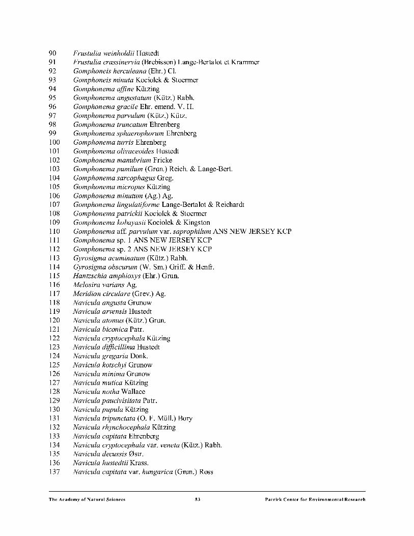
90 Frustulia weinholdii Hustedt 91 Frustulia crassinervia (Brebisson) Lange-Bertalot et Krammer 92 Gomphoneis herculean a (Ehr.) Cl. 93 Gomphoneis minuta Kociolek & Stoermer 94 Gomphonema affine Kiitzing 95 Gomphonema angustatum (Kiitz.) Rabh. 96 Gomphonema gracile Ehr. emend. V. H. 97 Gomphonema parvulum (Kiitz.) Kiitz. 98 Gomphonema truncatum Ehrenberg 99 Gomphonema sphaerophorum Ehrenberg 1 00 Gomphonema turris Ehrenberg 101 Gomphonema olivaceoides Hustedt 102 Gomphonema manubrium Fricke 103 Gomphonema pumilum (Grun.) Reich. & Lange-Bert. 1 04 Gomphonema sarcophagus Greg. 105 Gomphonema micro pus Kiitzing 106 Gomphonema minutum (Ag.) Ag. 107 Gomphonema lingulatiforme Lange-Bertalot & Reichardt 108 Gomphonema patrickii Kociolek & Stoermer 109 Gomphonema kobayasii Kociolek & Kingston 110 Gomphonema af£ parvulum var. saprophilum ANS NEW JERSEY KCP Ill Gomphonema sp. 1 ANS NEW JERSEY KCP 112 Gomphonema sp. 2 ANS NEW JERSEY KCP 113 Gyrosigma acuminatum (Kiitz.) Rabh. 114 Gyrosigma obscurum (W. Sm.) Griff. & Henfr. 115 Hantzschia amphioxys (Ehr.) Grun. 116 Melosira varians Ag. 117 Meridian circulare (Grev.) Ag. 118 Navicula angusta Grunow 119 Navicula arvensis Hustedt 120 Navicula atomus (Kiitz.) Grun. 121 Navicula biconica Patr. 122 Navicula cryptocephala Kiitzing 123 Navicula difficillima Hustedt 124 Navicula gregaria Donk. 125 Navicula kotschyi Grunow 126 Navicula minima Grunow 127 Navicula mutica Kiitzing 128 Navicula notha Wallace 129 Navicula paucivisitata Patr. 130 Navicula pupula Kiitzing 131 Navicula tripunctata (0. F. Miill.) Bory 132 Navicula rhynchocephala Kiitzing 133 Navicula capitata Ehrenberg 134 Navicula cryptocephala var. veneta (Kiitz.) Rabh. 135 Navicula decussis 0str. 136 Navicula hustedtii Krass. 137 Navicula capitata var. hungarica (Grun.) Ross


138 Navicula peregrina (Ehr.) Kiitz. 139 Navicula trivia/is Lange-Bert. 140 Navicula canalis Patr. 141 Navicula capitata var. lueneburgensis (Grun.) Patr. 142 Navicula ingenua Hustedt 143 Navicula integra (W. Sm.) Ra1fs 144 Navicula menisculus Schum. 145 Navicula placenta Ehrenberg 146 Navicula schroeteri var. escambia Patr. 147 Navicula secreta var. apiculata Patr. 148 Navicula salinarum Grunow 149 Navicula symmetrica Patr. 150 Navicula tenelloides Hustedt 151 Navicula tenera Hustedt 152 Navicula viridula var. rostellata (Kiitz.) Cl. 153 Navicula agrestis Hustedt 154 Navicula protracta (Grun.) Cl. 155 Navicula minuscula Grunow 156 Navicula heufleri var. leptocephala (Breb ex Grun.) Perag. 157 Navicula bacilloides Hustedt 158 Navicula absoluta Hustedt 159 Navicula veneta Kiitzing 160 Navicula longicephala Hustedt 161 Navicula molestiformis Hustedt 162 Navicula ignota var. acceptata (Hust.) Lange-Bert. 163 Navicula cryptotenella L.B. in Kramm. & L.-B. 164 Navicula perminuta Grunow 165 Navicula subminuscula Mang. 167 Navicula germainii Wallace 168 Navicula erifuga Lange-Bert. 169 Navicula recens Lange-Bert. 170 Navicula capitatoradiata Germain 171 Navicula atomus var. permitis (Hust.) Lange-Bert. 172 Navicula suchlandtii Hustedt 173 Navicula longicephala var. vilaplanii Lange-Berta1ot & Sa bater 175 Navicula lanceolata (Ag.) Ehr. 176 Navicula menisculus var. grunowii Lange-Berta1ot 177 Navicula ruttnerii var. capitata Hustedt 178 Navicula parabilis Hohn & Hellerman 179 Navicula sp. 1 ANS NEW JERSEY KCP 180 Neidium affine (Ehr.) Pfitz. 181 Neidium alpinum Hustedt 182 Nitzschia acicularioides Hustedt 183 Nitzschia acicularis (Kiitz.) W. Sm. 184 Nitzschia amphibia Grunow 185 Nitzschia capitellata Hustedt 186 Nitzschia dissipata (Kiitz.) Grun. 187 Nitzschia fonticola Grunow


188 Nitzschia frustulum (Kiitz.) Grun. 189 Nitzschia gracilis Hantz. ex Rabh. 190 Nitzschia heufleriana Grunow 191 Nitzschia linearis (Ag. ex W. Sm.) W. Sm. 192 Nitzschia microcephala Grunow 193 Nitzschia palea (Kiitz.) W. Sm. 194 Nitzschia palea var. tenuirostris Grunow 195 Nitzschia recta Hantz. ex Rabh. 196 Nitzschia sigma (Kiitz.) W. Sm. 197 Nitzschia dissipata var. media (Hantz.) Grun. 198 Nitzschia hungarica Grunow 199 Nitzschia inconspicua Grunow 200 Nitzschia perminuta (Grun.) Peragallo 201 Nitzschia clausii Hantz. 202 Nitzschia constricta var. subconstricta Grun. in Cl. et Grun. 203 Nitzschia filiformis (W. Sm.) V. H. 204 Nitzschia gracilis var. minor Skabitschevsky in Proschkina-Lavrenko 205 Nitzschia intermedia Hantz. ex Cl. et Grun. 206 Nitzschia liebethruthii Rabenhorst 207 Nitzschia littoralis Grun. inCl. et Grun. 208 Nitzschia lorenziana var. subtilis Grun. inCl. et Grun. 209 Nitzschia paleacea Grun. in V. H. 210 Nitzschia rosenstockii Lange-Berta1ot 211 Nitzschia tryblionella var. debilis (Arnott) Hust. 212 Nitzschia vermicularis (Kiitz.) Hantz. in Rabh. 213 Nitzschia brevissima Grun. in V. H. 214 Nitzschia commutata Grunow 215 Nitzschia sociabilis Hustedt 216 Nitzschia palea var. debilis (Kiitz.) Grun. 217 Nitzschia angustatula Lange-Bert. 218 Nitzschia sinuata var. delognei (Grun.) Lange-Bert. 219 Nitzschia flex aides Geit1er 220 Nitzschia acidoclinata Lange-Bert. 221 Nitzschia tubicola Grun. inCl. et Grun. 222 Nitzschia terrestris (Peterson) Hust. 223 Nitzschia coarctata Grunow 224 Nitzschia levidensis var. salinarum Grunow 225 Nitzschia lorenziana Grunow 226 Nitzschia levidensis var. victoriae Grunow 227 Nitzschia tryblionella var. salinarum Grun. inCl. et Grun. 228 Nitzschia aff.jonticola ANS NEW JERSEY KCP 229 Nitzschia archibaldii Lange-Berta1ot 230 Nitzschia sp. 1 ANS NEW JERSEY KCP 231 Nitzschia subconstricta Grunow 232 Pinnularia divergens W. Sm. 233 Pinnularia maior (Kiitz.) Rabh. 234 Pinnularia mesolepta (Ehr.) W. Sm. 235 Pinnularia microstauron (Ehr.) Cl.


236 Pinnularia obscura Krass. 237 Pinnularia rupestris Hautz. 238 Pinnularia subcapitata Greg. 239 Pinnularia lundii Hustedt 240 Pinnularia interrupta W. Sm. 241 Pinnularia parvulissima Kram. 242 Plagiotropis Iepidoptera var. proboscidea (Cl.) Reim. 243 Pleurosigma angulatum (Quek.) W. Sm. 244 Reimeria sinuata (Greg.) Kociolek & Stoermer 245 Rhoicosphenia curvata (Kiitz.) Grun. ex Rabh. 246 Stauroneis anceps Ehrenberg 24 7 Stauroneis smithii Grunow 248 Stauroneis phoenicenteron (Nitz.) Ehr. 249 Stauroneis agrestis Peters. 250 Stenopterobia intermedia (Lewis) V. H. 251 Stephanodiscus niagarae Ehrenberg 252 Stephanodiscus hantzschii Grunow 253 Stephanodiscus minutus H. L. Sm. 254 Surirella angusta Kiitzing 255 Surirella linearis W. Sm. 256 Surirella robusta Ehrenberg 257 Surirella stalagma Hohn & Hellerm. 258 Surirella minuta Breb. 259 Surirella brebissonii var. kuetzingii Kramm. & Lange-Bert. 260 Surirella brebissonii Kramm. & Lange-Bert. 261 Surirella amphioxys W. Sm. 262 Surirella splendida (Ehr.) Kiitz. 263 Synedra parasitic a (W. Sm.) Hust. 264 Synedra rumpens var. familiaris (Kiitz.) Hust. 265 Synedra ulna (Nitz.) Ehr. 266 Synedra ulna var. oxyrhynchus fo. mediocontracta (Fonti) Hust. 267 Synedra delicatissima var. angustissima Grunow 268 Synedra parasitica var. subconstricta (Grun.) Hust. 269 Tabellariaflocculosa (Roth) Kiitz. 270 Thalassiosira weissflogii (Grun.) Fryxell & Hasle 271 Pseudostaurosira brevistriata (Grun. in V.H.) Williams & Round 272 Bacillaria paradoxa Gmelin 273 Nupela neglecta Ponader, Lowe & Potapova 274 Nupela wellneri (Lange-Bert.) Lange-Bert. 275 Navicula sp. 2 ANS NEW JERSEY KCP 276 Navicula sp. 3 ANS NEW JERSEY KCP 277 Encyonema minutum (Hilse) Mann 278 Encyonema silesiacum (Bleisch) Mann 279 Encyonema prostratum (Berkeley) Kiitzing 280 Fallacia pygmaea (Kiitzing) Stickle et Mann 281 Fallacia auriculata (Hustedt) Mann 282 Fallacia omissa (Hustedt) Mann 283 Fallacia tenera (Hustedt) Mann


284 Karayevia clevei (Grunow) Round & Buktyiarova 285 Karayevia laterostrata (Hant.) Round and Bukt. 286 Luticola goeppertiana (Bleisch) Mann 287 Sellaphora seminulum (Grun.) Mann 288 Staurosira construens var. binodis (Ehrenberg) Hamilton 289 Staurosira construens var. venter (Ehr.) Hamilton 290 Staurosirella leptostauron (Ehrenberg) Williams et Round 291 Staurosirella pinnata (Her.) Williams & Round 292 Tryblionella apiculata Greg. 293 Tryblionella levidensis Wm. Sm. 294 Tryblionella aerophila 295 Psammothidium bioretii (Germ.) Bukht. et Round 296 Psammothidium subatomoides (Hustedt) Bukhtiyarova et Round 297 Psammothidium ventralis (Kras.) Bukht. et Round 298 Eucocconeis laevis (Oestrup) Lange-Bertalot 299 Fragilariforma constricta (Ehrenberg) Williams et Round 300 Fragilariforma virescens (Ralfs) Williams et Round 301 Placoneis clementis (Grun) Cox 302 Placoneis elginensis (Greg.) Cox 303 Placoneis explanata (Hust.) Cox 304 Cavinula pseudoscutiformis (Grunow ex Schmidt) Mann et Stickle 305 Diadesmis confervacea Kiitzing 306 Diadesmis contenta (Grunow ex Van Heurck) Mann


Appendix 3: Spearman's rank-order correlation for full dataset for both years (n=106)

Note: Waterchemistry: Cond, specific conductivity); NH3-N2); N03-N

2); TN, total nitrogen1

) (*TN calculated from combination of TKN1

) and N03-N2) ); TKN, total Kjeldahl nitrogen1); P04, orthophospate2

); TP, total phosphorus2l; Alk, alkalinitfl; Hard, hardness2l; pWl; DO, dissoved oxygen1l; General site characteristics: B _size, basin size; %0, percent open canopy cover; R_len, reach length; R_wid, average river width at reach; Flow, flow estimate in categories (1 =slow; 2=moderate; 3=fust); Substrate: %Bed, percent bedrock; %Bo, percent boulder; %Cob, percent cobble; %Gra, percent gravel; %S, percent sand; %Si/Cl, percent silt and clay, BRBDCOG, percent bedrock, boulder, cobble and gravel combined; SDSTCL, percent sand, silt and clay combined; BRBD, percent bedrock and boulder combined; CBGR, percent cobble and gravel combined; Biomass: AFDM, Ash free dry mass; Chl_a, chlorophyll a; 1ldata provided byNJ DEP and/or data records collected by NJ DEP and USGS at surface water monitoring stations, measured within a maxiumum of 4 weeks from algal sampling; 2lvariable measured by PCER Geochemistry section. Algal cover/biomass estimate: Rapid biomass assessment (REA). visual estimate o(percent cover ('Yr£stimated cover): %DGCov, %Dark Green (%estimated cover); %LsSCov, %Long spiny Spirogira (%estimated cover); %MdbCov, %Moss-like (Dark brown) (%estimated cover); %Bgs1Cov, blue-green (slimey) (%estimated cover), BlgrCov, %blue-green (%estimated cover); %BCCov, %Brown Coating (%estimated cover); %ChldCov, %Chladophora (%estimated cover); %Dfi1Cov, %Diatoms (filamentous) (%estimated cover); %DTBCov, %Diatoms (thin layer)+ Bare (%estimated cover); %GrFthCov, %Green (Feathery) (%estimated cover); %GrF1Cov, %Green Filamentous #1 (%estimated cover); %GrF2Cov, %Green Filamentous #2 (%estimated cover); %GFBCov, %Green Filamentous (Bushy) (%estimated cover); %GrFCov, %green filamentous (moss-like) (%estimated cover); %GrFsCov, %Green Fliamentous (Segemented branches) (%estimated cover); %HBCov, %Honey-Brown (%estimated cover); %LlGCov, %Long light green (%estimated cover); %0rgCov, %Orange (%estimated cover); %TgLCov, %thin green layer (%estimated cover); %TsCdCov, %Thin short Cladophera (%estimated cover); %GrBGCov, %Green (blue-green) (%estimated cover). Semi-quantitative count method (SQCM): percent estimate o(numbers o(cells (%

#cells): %DiatC, Diatoms(%# cell); %ChladC, Cladophora sp.(% #cell); %0egodC, Oedogonium sp.(% #cells); %RhizC, Rhizoclonium sp.(% #cells); %Scene, Scenedesmus sp.(% #cells); %SpirogC, Spirogyra sp.(% #cells); %MerismopC, Merismopedia sp.(% #cells); %0scillC, Oscillatoria sp.(% #cells); %AudouC, Audouinella sp.(% #cells);

p- value: ** correlation significant at the 0.01 level (2-tailed test) * correlation significant at the 0.05 level (2-tailed test)

NH,_N PO, TP Chl_a AFDM R_wid R_len Flow

NO,-N 0.32 ** 0.45 4** 0.383** 0.115 0.261 ** 0.141 0.222* -0.176 r

0 0 0 0.242 0.00703 0.149 0.0226 0.0718 p-value

NH,-N 0.233* 0.36 6** -0.164 0.113 -0.161 -0.232* -0.0547 r

0.0165 0 0.0939 0.247 0.0987 0.0169 0.577 p-value

PO, 0.95 ** 0.167 0.0637 0.374** 0.207* 0.236* r

0 0.0873 0.516 0 0.0338 0.0151 p-value

TP 0.127 0.0679 0.361 ** 0.138 0.235* r

0.195 0.488 0 0.159 0.0156 p-value

Chl_a 0. 716** 0.40 8** 0.341 ** 0.0771 r

0 0 0 0.431 p-value

AFDM 0.251 ** 0.222* -0.141 r

0.00968 0.0224 0.15 p-value

R_wid 0. 75 7** 0.28 ** r

0 0.00373 p-value

R_len 0.143 r

0.144


NO,-N

NH,-N

PO,

TP

chl_a

AFDM

R_wid

R_len

Flow

B_size

DO

pH

Cond

%0

%DiatC

%ChladC

NO,-N

NH,-N

PO,

TP

Chl_a

AFDM

R_wid

R_len

Flow

B size

0.0397

0.703

-0.105

0.315

0.177

0.0881

0.164

0.115

0.0261

0.803

-0.0869

0.404

0.14

0.179

0.0535

0.608

0.145

0.163

%RhizC

-0.063

0.52

0.11

0.26

0.123

0.209

0.116

0.236

0.00552

0.955

-0.0399 0.684

-0.06

0.541

-0.0562

0.567

0.116

0.236

DO

-0.0901

0.358

-0.648**

0

0.047

0.632

-0.0382

0.697

0.177

0.0688

-0.115

0.24

0.191 *

0.0497

0.36 8**

0

0.0652

0.506

0.0984

0.345

%Scene

-0.0877

0.37

0.0303

0.757

-0.00957

0.922

0.0239

0.807

0.0909

0.353

0.0941

0.337

0.0528

0.59

-0.0112

0.909

-0.0802

0.413

The Academy of Nat ural Sciences

pH

-0.28 9**

0.00273

-0.243*

0.0121

-0.00448

0.964

-0.0374

0.703

0.107

0.274

-0.199*

0.0413

0.227*

0.0193

0.159

0.104

0.13

0.183

0.0783

0.452

0.55 6**

0

Cond

0.215*

0.0267

0.43 I**

0

0.49 2**

0

0.49 7**

0

0.0663

0.499

0.0155

0.875

0.084

0.391

0.0377

0.701

-0.0581

0.554

0.215*

0.0371

-0.0358

0.715

0.31 **

0.00128

%0

0.0125

0.899

-0.199*

0.0405

0.195*

0.0449

0.158

0.106

0.42 **

0

0.241 *

0.013

0.69 8**

0

0.606**

0

0.2*

0.0401

0.222*

0.0314

0.209*

0.0315

0.209*

0.0316

0.0671

0.494

% SpirogC % M erismoC % OscillC

-0.136

0.165

0.0942

0.336

-0.0303

0.757

-0.0399

0.684

-0.107

0.275

-0.0813

0.407

-0.165

0.0915

-0.135

0.168

-0.147

0.132

0.0638

0.515

0.0383

0.696

-0.0223

0.82

0.016

0.871

-0.0144

0.884

0.0367

0.708

-0.032

0.744

-0.162

0.0972

-0.0802

0.413

59

-0.11

0.261

0

0.0502

0.609

0.0502

0.609

0.0971

0.322

0.0712

0.468

-0.0162

0.869

-0.0561

0.567

-0.0331

0.736

%DiatC

0.152

0.12

-0.0245

0.803

0.174

0.0739

0.158

0.106

0.216*

0.0264

0.152

0.12

0.26 9**

0.00535

0.26 8**

0.00551

0.0487

0.619

-0.0196

0.851

0.0211

0.83

-0.0355

0.717

0.158

0.105

0.21 *

0.0307

%ChladC %0egodC

-0.0996

0.309

-0.128

0.192

-0.115

0.24

-0.0953

0.331

0.246*

0.0112

0.127

0.194

0.222*

0.0222

0.229*

0.0184

0.0589

0.548

0.0191

0.854

0.252**

0.00918

0.32 8**

0

-0.0353

0.719

0.28 8**

0.00282

-0.0925

0.345

0.0443

0.652

-0.0386

0.694

0.107

0.274

0.112

0.252

0.18

0.0644

0.219*

0.0244

0.0588

0.549

0.0265

0.787

-0.178

0.0672

-0.0744

0.475

0.0944

0.335

-0.014

0.886

0.0227

0.817

-0.0382

0.697

0.0338

0.731

-0.0608

r

p-value

r

p-value

r

p-value

r

p-value

r

p-value

r

p-value

r

p-value

r

p-value

r

p-value

r

p-value

r

p-value

r

p-value

r

p-value

r

p-value

r

p-value

r

0.535 p-value

%AudouC %DGCov %LsSCov

0.136

0.164

0.235*

0.0157

-0.111

0.258

-0.0976

0.319

-0.0612

0.533

0.0507

0.605

0.0272

0.781

-0.0352

0.72

0.0866

0.376

-0.0363

0.712

0.114

0.242

-0.271 **

0.00513

-0.22*

0.0233

-0.122

0.213

0.148

0.13

-0.213*

0.0289

-0.171

0.0796

0.0526

0.592

-0.193*

0.0479

0.134

0.171

-0.0431

0.661

-0.0567

0.563

-0.186

0.0561

-0.159

0.103

-0.234*

0.0159

-0.191 *

0.0495

-0.161

0.099

r

p-value

r

p-value

r

p-value

r

p-value

r

p-value

r

p-value

r

p-value

r

p-value

r

p-value

Patrick Center for Environmental Research

B_size

DO

pH

Cond

%0

%DiatC

%ChladC

%0egodC

%RhizC

%Scene

%SpirogC

%Merismopl

% OscillC

%AudouC

%DGCov

NO,-N

NH,-N

PO,

TP

chi_ a

AFDM

R_wid

R_len

Flow

B_size

DO

%RhizC

-0.0936

0.369

-0.0254

0.796

0.0359

0.714

0.145

0.137

0.0708

0.47

0.0275

0.78

-0.0494

0.614

-0.0237

0.809

%Scene

0.0861

0.409

-0.0942

0.336

-0.0208

0.832

0.0526

0.591

-0.0383

0.696

0.0193

0.844

-0.0348

0.723

-0.0167

0.865

-0.0135

0.89

%MdhCov %BGslCov

-0.0363 0.0307

0.712 0.754

0.114 -0.17

0.242 0.0809

-0.271 ** -0.0698

0.00513 0.477

-0.22*

0.0233

-0.12

0.221

0.152

0.12

-0.213*

0.0289

-0.171

0.0801

0.0526

0.592

-0.1

0.335

-0.246*

0.0113

-0.137

0.162

0.205*

0.0347

0.125

0.2

0.227*

0.0197

0.261 **

0.00706

0.0526

0.592

0.211 *

0.0413

0.262**

0.00669


%SpirogC

0.0574

0.582

-0.117

0.234

-0.0978

0.318

0.164

0.0922

0.0431

0.66

0.0193

0.844

-0.0348

0.723

-0.0167

0.865

-0.0135

0.89

-0.00952

0.923

%BlgrCov

-0.106

0.279

-0.31 **

0.00129

0.16

0.1

0.0527

0.591

0.247*

0.0107

0.0843

0.39

0.197*

0.0426

0.15

0.124

0.192*

0.0486

-0.133

0.201

0.248*

0.0105

%MerismoC

-0.119

0.254

-0.0942

0.336

-0.0577

0.556

0.0207

0.833

-0.0718

0.464

0.0193

0.844

-0.0348

0.723

-0.0167

0.865

-0.0135

0.89

-0.00952

0.923

-0.00952

0.923

%BCCov

-0.126

0.198

-0.121

0.215

-0.0973

0.32

-0.112

0.254

0.12

0.222

-0.123

0.209

0.154

0.116

0.159

0.104

0.132

0.177

-0.0287

0.783

0.0686

0.484

60

% OscillC

-0.00389

0.97

-0.00081

0.993

0.0195

0.842

0.136

0.164

0.0324

0.741

0.0392

0.689

-0.0706

0.471

-0.0338

0.73

-0.0275

0.78

-0.0193

0.844

-0.0193

0.844

-0.0193

0.844

%ChldCov

0.0231

0.813

-0.00124

0.99

0.164

0.0922

0.137

0.161

0.403**

0

0.124

0.206

0.173

0.076

0.197*

0.0429

0.175

0.0736

0.00971

0.926

0.103

0.291

%AudouC

-0.101

0.334

-0.28 9**

0.00271

-0.192*

0.0489

-0.0409

0.677

-0.0688

0.483

-0.105

0.283

-0.0286

0.771

-0.058

0.554

-0.0471

0.631

-0.0332

0. 735

-0.0332

0. 735

-0.0332

0. 735

-0.0673

0.493

%DFilCov

0.245*

0.0114

0.149

0.128

0.137

0.162

0.144

0.141

-0.0177

0.857

0.0469

0.632

-0.136

0.163

-0.188

0.0543

-0.441 **

0

0.108

0.298

-0.0579

0.555

%DGCov

-0.1

0.335

-0.246*

0.0113

-0.247*

0.0109

-0.28 7**

0.0029

-0.0109

0.912

0.0338

0.731

-0.0608

0.535

-0.0291

0.767

-0.0237

0.809

-0.0167

0.865

-0.0167

0.865

-0.0167

0.865

-0.0338

0.73

0.113

0.25

%LsSCov

0.132

0.203

-0.166

0.0897

-0.139

0.155

0.233*

0.0161

-0.0326

0.739

0.0275

0.78

-0.0494

0.614

-0.0237

0.809

-0.0192

0.845

-0.0135

0.89

0.69 7**

0

-0.0135

0.89

-0.0275

0.78

-0.0471

0.631

-0.0237

r

p-value

r

p-value

r

p-value

r

p-value

r

p-value

r

p-value

r

p-value

r

p-value

r

p-value

r

p-value

r

p-value

r

p-value

r

p-value

r

p-value

r

0.81 p-value

% DTBCov %GrFthCov

-0.239*

0.0138

-0.187*

0.0556

-0.183

0.0602

-0.16

0.102

-0.186

0.0561

-0.193*

0.0476

0.0784

0.424

0.123

0.207

0.389**

0

-0.117

0.261

0.132

0.176

0.0307

0.754

-0.17

0.0809

-0.0698

0.477

-0.137

0.162

0.205*

0.0347

0.125

0.2

0.227*

0.0197

0.261 **

0.00706

0.0526

0.592

0.211 *

0.0413

0.262**

0.00669

r

p-value

r

p-value

r

p-value

r

p-value

r

p-value

r

p-value

r

p-value

r

p-value

r

p-value

r

p-value

r

p-value


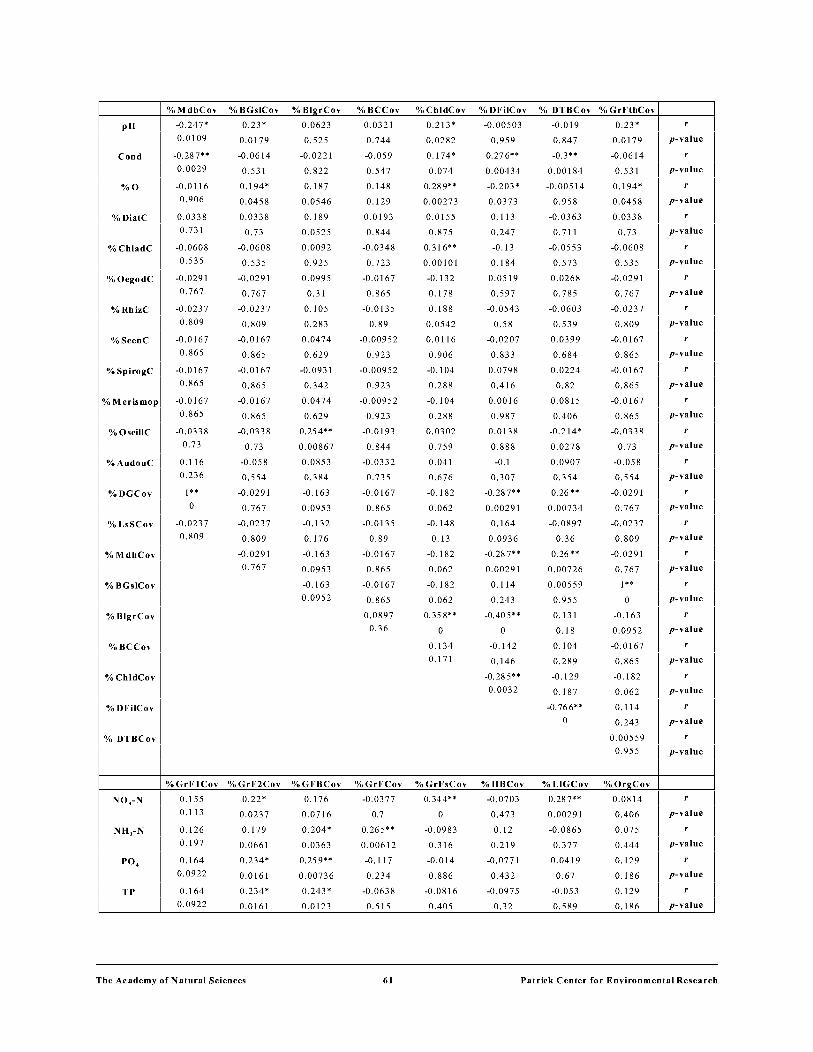
I %MdbCov %BGslCov %BlgrCov %BCCov %CbldCov %DFilCov % DTBCov %GrFtbCov I I pH

Cond

%0

%DiatC

%CbladC

%0egodC

%RbizC

%Scene

%SpirogC

-0.247*

0.0109

-0.28 7**

0.0029

-0.0116

0.906

0.0338

0.731

-0.0608

0.535

-0.0291

0.767

-0.0237

0.809

-0.0167

0.865

-0.0167

0.865

%Merismop -0.0167

% OscillC

%AudouC

%DGCov

%LsSCov

%MdbCov

%BGslCov

%BlgrCov

%BCCov

%CbldCov

%DFilCov

% DTBCov

NO,-N

NH,-N

PO,

TP

0.865

-0.0338

0.73

0.116

0.236

I**

0

-0.0237

0.809

I %GrF1Cov

1 o.l55

1 o.ll3

1 o.l26

1 o.l97

1 o.l64

Il

l 0.0922

0.164

0.0922

0.23*

0.0179

-0.0614

0.531

0.194*

0.0458

0.0338

0.73

-0.0608

0.535

-0.0291

0.767

-0.0237

0.809

-0.0167

0.865

-0.0167

0.865

-0.0167

0.865

-0.0338

0.73

-0.058

0.554

-0.0291

0.767

-0.0237

0.809

-0.0291

0.767

%GrF2Cov

0.22*

0.0237

0.179

0.0661

0.234*

0.0161

0.234*

0.0161


0.0623

0.525

-0.0221

0.822

0.187

0.0546

0.189

0.0525

0.0092

0.925

0.0995

0.31

0.105

0.283

0.0474

0.629

-0.0931

0.342

0.0474

0.629

0.254**

0.00867

0.0853

0.384

-0.163

0.0953

-0.132

0.176

-0.163

0.0953

-0.163

0.0952

%GFBCov

0.176

0.0716

0.204*

0.0363

0.25 9**

0.00736

0.243*

0.0123

0.0321

0.744

-0.059

0.547

0.148

0.129

0.0193

0.844

-0.0348

0.723

-0.0167

0.865

-0.0135

0.89

-0.00952

0.923

-0.00952

0.923

-0.00952

0.923

-0.0193

0.844

-0.0332

0. 735

-0.0167

0.865

-0.0135

0.89

-0.0167

0.865

-0.0167

0.865

0.0897

0.36

%GrFCov

-0.0377

0.7

0.265**

0.00612

-0.117

0.234

-0.0638

0.515

61

0.213*

0.0282

0.174*

0.074

0.28 9**

0.00273

0.0155

0.875

0.316**

0.00101

-0.132

0.178

0.188

0.0542

0.0116

0.906

-0.104

0.288

-0.104

0.288

0.0302

0.759

0.041

0.676

-0.182

0.062

-0.148

0.13

-0.182

0.062

-0.182

0.062

0.35 8**

0

0.134

0.171

%GrFsCov

0.344**

0

-0.0983

0.316

-0.014

0.886

-0.0816

0.405

-0.00503

0.959

0.27 6**

0.00434

-0.203*

0.0373

0.113

0.247

-0.13

0.184

0.0519

0.597

-0.0543

0.58

-0.0207

0.833

0.0798

0.416

0.0016

0.987

0.0138

0.888

-0.1

0.307

-0.28 7**

0.00291

0.164

0.0936

-0.28 7**

0.00291

0.114

0.243

-0.40 5**

0

-0.142

0.146

-0.285**

0.0032

%HBCov

-0.0703

0.473

0.12

0.219

-0.0771

0.432

-0.0975

0.32

-0.019

0.847

-0.3**

0.00184

-0.00514

0.958

-0.0363

0.711

-0.0553

0.573

0.0268

0.785

-0.0603

0.539

0.0399

0.684

0.0224

0.82

0.0815

0.406

-0.214*

0.0278

0.0907

0.354

0.26 **

0.00734

-0.0897

0.36

0.26 **

0.00726

0.00559

0.955

0.131

0.18

0.104

0.289

-0.129

0.187

-0.76 6**

0

%LIGCov

0.28 7**

0.00291

-0.0865

0.377

0.0419

0.67

-0.053

0.589

0.23*

0.0179

-0.0614

0.531

0.194*

0.0458

0.0338

0.73

-0.0608

0.535

-0.0291

0.767

-0.0237

0.809

-0.0167

0.865

-0.0167

0.865

-0.0167

0.865

-0.0338

0.73

-0.058

0.554

-0.0291

0.767

-0.0237

0.809

-0.0291

0.767

I**

0

-0.163

0.0952

-0.0167

0.865

-0.182

0.062

0.114

0.243

0.00559

r

p-value

r

p-value

r

p-value

r

p-value

r

p-value

r

p-value

r

p-value

r

p-value

r

p-value

r

p-value

r

p-value

r

p-value

r

p-value

r

p-value

r

p-value

r

p-value

r

p-value

r

p-value

r

p-value

r

p-value

r

0.955 p-value

%0rgCov I o.o814 1 r

0.406 p-value

0.075 r

0.444 p-value

0.129 r

0.186 p-value

0.129 r

0.186 p-value

I


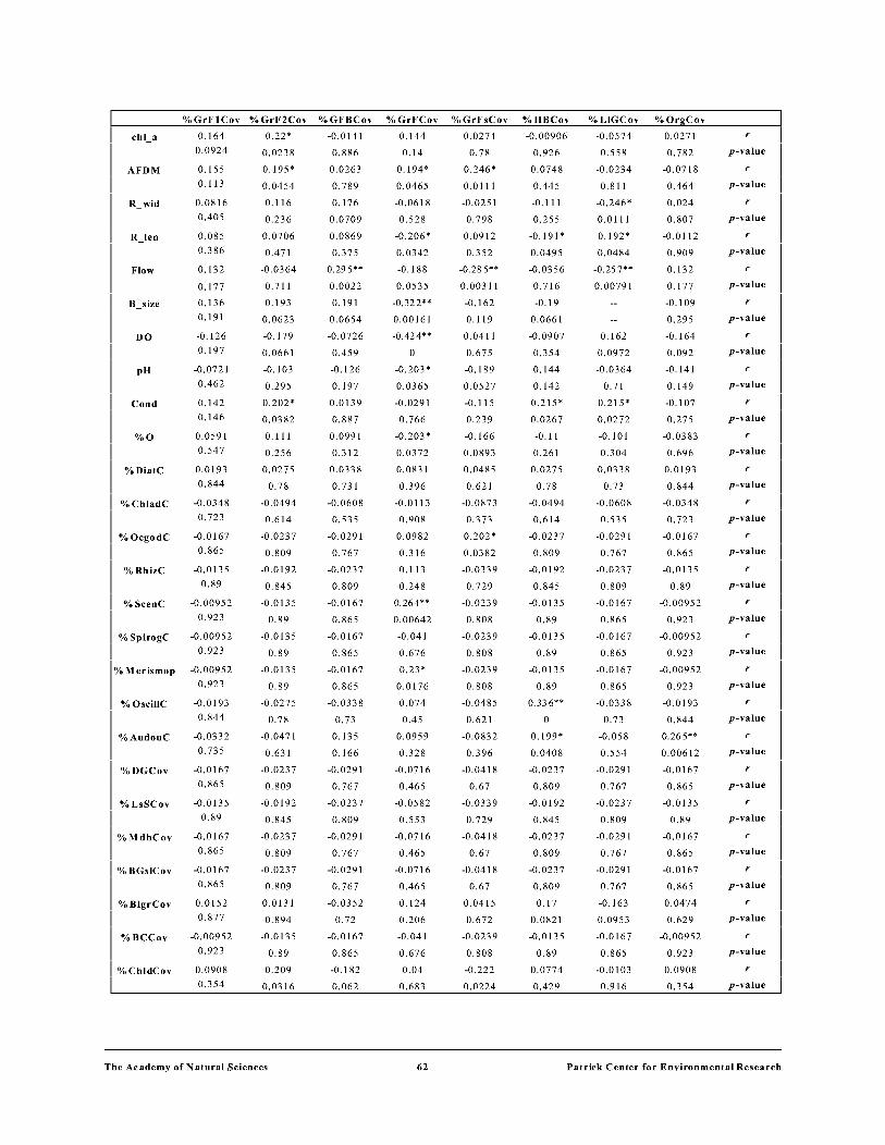
%GrF1Cov %GrF2Cov %GFBCov %GrFCov %GrFsCov %HBCov %LIGCov %0rgCov

chi_ a

AFDM

R_wid

R_len

Flow

B size

DO

pH

Cond

%0

%DiatC

%ChladC

%0egodC

0.164

0.0924

0.155

0.113

0.0816

0.405

0.085

0.386

0.132

0.177

0.136

0.191

-0.126

0.197

-0.0721

0.462

0.142

0.146

0.0591

0.547

0.0193

0.844

-0.0348

0.723

-0.0167

0.865

%RhizC -0.0135

0.89

%Scene -0.00952

0.923

% SpirogC -0.00952

0.923

%Merismop -0.00952

0.923

%0scillC -0.0193

0.844

%AudouC -0.0332

0. 735

%DGCov -0.0167

0.865

%LsSCov -0.0135

0.89

%MdhCov -0.0167 0.865

%BGslCov -0.0167 0.865

%BlgrCov 0.0152 0.877

% BCCov -0.00952

0.923

% ChldCov 0.0908 0.354

0.22*

0.0238

0.195*

0.0454

0.116

0.236

0.0706

0.471

-0.0364

0.711

0.193

0.0623

-0.179

0.0661

-0.103

0.295

0.202*

0.0382

0.111

0.256

0.0275

0.78

-0.0494

0.614

-0.0237

0.809

-0.0192

0.845

-0.0135

0.89

-0.0135

0.89

-0.0135

0.89

-0.0275

0.78

-0.0471

0.631

-0.0237

0.809

-0.0192

0.845

-0.0237

0.809

-0.0237

0.809

0.0131

0.894

-0.0135

0.89

0.209

0.0316


-0.0141

0.886

0.0263

0.789

0.176

0.0709

0.0869

0.375

0.295**

0.0022

0.191

0.0654

-0.0726

0.459

-0.126

0.197

0.0139

0.887

0.0991

0.312

0.0338

0.731

-0.0608

0.535

-0.0291

0.767

-0.0237

0.809

-0.0167

0.865

-0.0167

0.865

-0.0167

0.865

-0.0338

0.73

0.135

0.166

-0.0291

0.767

-0.0237

0.809

-0.0291

0.767

-0.0291

0.767

-0.0352

0.72

-0.0167

0.865

-0.182

0.062

0.144

0.14

0.194*

0.0465

-0.0618

0.528

-0.206*

0.0342

-0.188

0.0535

-0.322**

0.00161

-0.424**

0

-0.203*

0.0365

-0.0291

0.766

-0.203*

0.0372

0.0831

0.396

-0.0113

0.908

0.0982

0.316

0.113

0.248

0.264**

0.00642

-0.041

0.676

0.23*

0.0176

0.074

0.45

0.0959

0.328

-0.0716

0.465

-0.0582

0.553

-0.0716

0.465

-0.0716

0.465

0.124

0.206

-0.041

0.676

0.04

0.683

62

0.0274

0.78

0.246*

0.0111

-0.0251

0.798

0.0912

0.352

-0.285**

0.00311

-0.162

0.119

0.0411

0.675

-0.189

0.0527

-0.115

0.239

-0.166

0.0893

0.0485

0.621

-0.0873

0.373

0.202*

0.0382

-0.0339

0.729

-0.0239

0.808

-0.0239

0.808

-0.0239

0.808

-0.0485

0.621

-0.0832

0.396

-0.0418

0.67

-0.0339

0.729

-0.0418

0.67

-0.0418

0.67

0.0415

0.672

-0.0239

0.808

-0.222

0.0224

-0.00906

0.926

0.0748

0.445

-0.111

0.255

-0.191 *

0.0495

-0.0356

0.716

-0.19

0.0661

-0.0907

0.354

0.144

0.142

0.215*

0.0267

-0.11

0.261

0.0275

0.78

-0.0494

0.614

-0.0237

0.809

-0.0192

0.845

-0.0135

0.89

-0.0135

0.89

-0.0135

0.89

0.33 6**

0

0.199*

0.0408

-0.0237

0.809

-0.0192

0.845

-0.0237

0.809

-0.0237

0.809

0.17

0.0821

-0.0135

0.89

0.0774

0.429

-0.0574

0.558

-0.0234

0.811

-0.246*

0.0111

0.192*

0.0484

-0.25 7**

0.00791

0.162

0.0972

-0.0364

0.71

0.215*

0.0272

-0.101

0.304

0.0338

0.73

-0.0608

0.535

-0.0291

0.767

-0.0237

0.809

-0.0167

0.865

-0.0167

0.865

-0.0167

0.865

-0.0338

0.73

-0.058

0.554

-0.0291

0.767

-0.0237

0.809

-0.0291

0.767

-0.0291

0.767

-0.163

0.0953

-0.0167

0.865

-0.0103

0.916

0.0271

0.782

-0.0718

0.464

0.024

0.807

-0.0112

0.909

0.132

0.177

-0.109

0.295

-0.164

0.092

-0.141

0.149

-0.107

0.275

-0.0383

0.696

0.0193

0.844

-0.0348

0.723

-0.0167

0.865

-0.0135

0.89

-0.00952

0.923

-0.00952

0.923

-0.00952

0.923

-0.0193

0.844

0.265**

0.00612

-0.0167

0.865

-0.0135

0.89

-0.0167

0.865

-0.0167

0.865

0.0474

0.629

-0.00952

0.923

0.0908

0.354

r

p-value

r

p-value

r

p-value

r

p-value

r

p-value

r

p-value

r

p-value

r

p-value

r

p-value

r

p-value

r

p-value

r

p-value

r

p-value

r

p-value

r

p-value

r

p-value

r

p-value

r

p-value

r

p-value

r

p-value

r

p-value

r

p-value

r

p-value

r

p-value

r

p-value

r

p-value


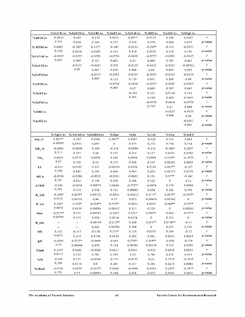
%GrF1Cov %GrF2Cov %GFBCov %GrFCov %GrFsCov %HBCov %LIGCov %0rgCov

I % DFilCov -0.0925

1 o.345

I% DTBCov 0.0607

1 o.536

%GrFthCov -0.0167

%GrF1Cov

%GrF2Cov

%GFBCov

%GrFCov

%GrFsCov

%HBCov

%LIGCov

NO,-N

NH,-N

PO,

TP

chi_ a

AFDM

R_wid

R_len

Flow

B size

DO

pH

Cond

%0

%DiatC

0.865

%TgLCov

0.28 7**

0.00291

-0.0865

0.377

0.0418

0.67

-0.053

0.589

-0.0594

0.545

-0.026

0.791

-0.246*

0.0111

0.193*

0.0478

-0.25 7**

0.00791

0.162

0.0972

-0.0364

0.71

0.215*

0.0272

-0.102

0.296

0.0338

0.731

-0.005

0.959

-0.209*

0.0318

-0.0237

0.809

-0.0135

0.89

-0.135

0.166

0.213*

0.0283

-0.0291

0.767

-0.0167

0.865

-0.0237

0.809

% TsCdCov % GrBGCov

-0.187

0.0551

-0.0698

0.477

0.0251

0.798

-0.0195

0.842

-0.0206

0.833

-0.0634

0.518

0.26 8**

0.00551

0.239*

0.0139

0.111

0.255

-0.112

0.254

0.255**

0.00844

0.0363

0.712

0.172

0.0774

0.0338

0.73

0.0398

0.685

0.104

0.29

0.0974

0.32

0.131

0.182

-0.0315

0.748

0.00935

0.924

0.00733

0.94

-0.254**

0.00885

0.00761

0.938

-0.00764

0.942

-0.174

0.0748

-0.0696

0.478

-0.0268

0.785

-0.0248

0.8

-0.254**

0.00887


0.0641

0.513

-0.142

0.145

-0.0716

0.465

-0.041

0.676

-0.0582

0.553

-0.0716

0.465

%Bed

0.363**

0

-0.156

0.111

0.106

0.279

0.00418

0.966

-0.0101

0.918

0.0644

0.511

-0.0955

0.33

0.27 5**

0.00437

-0.245*

0.0114

-0.273**

0.00788

0.237*

0.0144

-0.061

0.534

0.0257

0.793

-0.123

0.207

0.0565

0.564

63

0.0977

0.318

-0.0151

0.878

-0.0418

0.67

-0.0239

0.808

-0.0339

0.729

-0.0418

0.67

-0.103

0.294

%Bo

0.0207

0.833

-0.0984

0.315

0.0829

0.398

0.0142

0.885

-0.0832

0.396

-0.25 7**

0.00802

-0.00311

0.975

-0.0621

0.527

0.231 *

0.0174

0.168

0.106

0.125

0.203

0.27 9**

0.00391

0.0915

0.35

-0.0575

0.557

-0.0699

0.476

0.0544

0.579

-0.209*

0.0318

-0.0237

0.809

-0.0135

0.89

-0.0192

0.845

-0.0237

0.809

0.135

0.169

-0.0339

0.729

%Cob

-0.122

0.212

-0.153

0.117

0.0909

0.353

0.0738

0.452

0.151

0.122

-0.0434

0.658

0.27 7**

0.00418

0.0957

0.329

0.382**

0

0.341 **

0

0.0723

0.461

0.30 8**

0.00139

-0.025

0.798

0.16

0.101

-0.0484

0.622

0.169

0.084

-0.121

0.218

-0.0291

0.767

-0.0167

0.865

-0.0237

0.809

-0.0291

0.767

-0.0716

0.465

-0.0418

0.67

-0.0237

0.809

%Gra

0.112

0.254

-0.206*

0.0341

0.316**

0.00102

0.285**

0.00317

0.33 **

0

0.158

0.106

0.283**

0.00342

0.344**

0

0.063

0.521

0.0748**

0.473

0.198

0.0415

-0.036

0.713

0.0638

0.515

0.231 *

0.0175

0.229*

0.0181

0.0207

0.833

-0.0527

0.591

-0.0167

0.865

-0.00952

0.923

-0.0135

0.89

-0.0167

0.865

0.192

0.0487

-0.0239

0.808

-0.0135

0.89

-0.0167

r

p-value

r

p-value

r

p-value

r

p-value

r

p-value

r

p-value

r

p-value

r

p-value

r

p-value

r

0.865 p-value

%Si/Cl

0.064

0.514

0.202*

0.0382

-0.197*

0.0428

-0.23*

0.0179

-0.141

0.15

0.0904

0.356

-0.33 8**

0

-0.29 **

0.00261

-0.33 **

0

-0.17

0.101

-0.17

0.0814

-0.176

0.0705

0.0412

0.675

-0.192*

0.0485

-0.197*

0.0431

r

p-value

r

p-value

r

p-value

r

p-value

r

p-value

r

p-value

r

p-value

r

p-value

r

p-value

r

p-value

r

p-value

r

p-value

r

p-value

r

p-value

r

p-value


% TgLCov % TsCdCov % GrBGCov

%ChladC

%0egodC

-0.0608

0.535

-0.0291

0.767

%RhizC -0.0237

0.809

%Scene -0.0167

0.865

%SpirogC -0.0167 0.865

%Merismop -0.0167 0.865

%0scillC -0.0338

0.73

%AudouC -0.058 0.554

%DGCov -0.0291

0.767

%LsSCov -0.0237 0.809

%MdhCov -0.0291 0.767

% BGsiCov -0.0291 0.767

%BigrCov -0.163 0.0953

%BCCov -0.0167

0.865

%ChldCov -0.0108 0.913

%Dfi1Cov 0.168 0.0853

% DTBCov -0.12 0.222

%GrFthCov -0.0291

%GrF1Cov

%GrF2Cov

%GFBCov

%GrFCov

%GrFsCov

%HBCov

%LIGCov

%0rgCov

0.767

-0.0167

0.865

-0.0237

0.809

-0.0291

0.767

-0.0716

0.465

-0.0418

0.67

-0.0237

0.809

I**

0

-0.0167

0.865

0.118

0.227

-0.0291

0.767

-0.0237

0.809

-0.0167

0.865

-0.0167

0.865

-0.0167

0.865

-0.0338

0.73

-0.058

0.554

-0.0291

0.767

-0.0237

0.809

-0.0291

0.767

-0.0291

0.767

-0.163

0.0953

-0.0167

0.865

-0.126

0.199

-0.143

0.143

0.0617

0.529

-0.0291

0.767

-0.0167

0.865

-0.0237

0.809

-0.0291

0.767

-0.0716

0.465

-0.0418

0.67

-0.0237

0.809

-0.0291

0.767

-0.0167

0.865


-0.0608

0.535

-0.0291

0.767

-0.0237

0.809

-0.0167

0.865

-0.0167

0.865

-0.0167

0.865

-0.0338

0.73

0.14

0.151

-0.0291

0.767

-0.0237

0.809

-0.0291

0.767

-0.0291

0.767

-0.163

0.0953

-0.0167

0.865

-0.00223

0.982

0.205*

0.0355

-0.25 7**

0.00796

-0.0291

0.767

-0.0167

0.865

-0.0237

0.809

-0.0291

0.767

-0.0716

0.465

-0.0418

0.67

-0.0237

0.809

-0.0291

0.767

-0.0167

0.865

%Bed

-0.102

0.298

0.166*

0.0882

-0.0396

0.686

-0.0279

0.776

-0.0279

0.776

-0.0279

0.776

-0.0565

0.564

-0.097

0.322

-0.0487

0.619

-0.0396

0.686

-0.0487

0.619

-0.0487

0.619

0.0515

0.6

-0.0279

0.776

-0.064

0.514

0.175

0.072

-0.113

0.248

-0.0487

0.619

-0.0279

0.776

-0.0396

0.686

-0.0487

0.619

-0.12

0.221

0.372**

0

-0.0396

0.686

0.585**

0

-0.0279

0.776

64

%Bo

-0.0802

0.413

-0.0403

0.681

-0.0515

0.6

-0.123

0.208

-0.00811

0.934

-0.00811

0.934

-0.0642

0.513

0.156

0.11

-0.215*

0.0267

0.106

0.279

-0.215*

0.0267

0.17

0.0812

0.00911

0.926

0.123

0.208

-0.0631

0.52

0.0903

0.356

0.056

0.568

0.17

0.0812

0.133

0.174

-0.134

0.17

0.172

0.0779

-0.202

0.0379

0.0195

0.843

0.0369

0.707

-0.0142

0.885

0.0973

0.321

%Cob

0.203*

0.037

-0.0283

0.773

-0.0902

0.357

0.0752

0.443

-0.131

0.18

-0.04

0.684

-0.026

0.791

0.126

0.196

-0.25 8**

0.00769

-0.0705

0.472

-0.25 8**

0.00771

0.131

0.179

0.172

0.0781

-0.0624

0.525

0.19

0.0506

0.00391

0.968

-0.0635

0.517

0.131

0.179

0.118

0.227

-0.161

0.0999

0.0893

0.362

-0.034

0.729

-0.162

0.0974

-0.00682

0.945

-0.185

0.0583

0.162

0.098

%Gra

0.0744

0.448

0.149

0.126

0.0631

0.52

0.139

0.154

-0.096

0.327

0.096

0.327

0.0795

0.417

-0.21

0.031

-0.187

0.0553

-0.136

0.163

-0.188

0.0536

0.0476

0.628

0.209*

0.0319

0.056

0.568

0.199*

0.0413

-0.209*

0.032

0.15

0.125

0.0476

0.628

0.0272

0.782

-0.0214

0.827

0.0947

0.334

-0.0224

0.819

0.114

0.244

-0.156

0.111

0.0984

0.315

-0.0304

0.757

%S

-0.109

0.264

-0.0677

0.49

0.137

0.161

-0.102

0.296

0.141

0.15

0.0479

0.625

0.0454

0.644

0.0149

0.879

0.274**

0.00464

0.0256

0.794

0.274**

0.00461

-0.129

0.189

-0.0666

0.497

0.00799

0.935

0.0191

0.846

0.0564

0.565

-0.163

0.0942

-0.129

0.189

-0.136

0.165

0.182

0.0623

-0.26 9**

0.00541

0.0908

0.354

0.0896

0.361

0.162

0.0963

0.0345

0.725

-0.136

0.165

r

p-value

r

p-value

r

p-value

r

p-value

r

p-value

r

p-value

r

p-value

r

p-value

r

p-value

r

p-value

r

p-value

r

p-value

r

p-value

r

p-value

r

p-value

r

p-value

r

p-value

r

p-value

r

p-value

r

p-value

r

p-value

r

p-value

r

p-value

r

p-value

r

p-value

r

p-value


I %TgLCov

I %TgLCov

I %TsCdCov

I %GrBGCov

%Bed

%Bo

%Cob

%Gra

NO,-N

NH,-N

PO,

TP

cbl_a

AFDM

R_wid

R_len

Flow

B_size

DO

pH

COND

%0

%DiatC

%CbladC

%0egodC

%RbizC

%Si/Cl

0.0177

0.857

-0.105

0.281

-0.0434

0.658

-0.049

0.618

-0.113

0.248

-0.0469

0.632

0.00415

0.966

0.216

0.026

-0.311 **

0.00123

-0.235*

0.023

0.27 **

0.00516

0.117

0.233

-0.0148

0.88

0.0396

0.687

-0.182

0.0614

0.103

0.294

0.0502

0.608

-0.0838

0.393

% TsCdCov % GrBGCov

-0.0291

0.767

-0.0291

0.767

-0.0291

0.767

BRBDCOG SDSTCL

-0.0571

0.561

-0.22*

0.0234

0.233*

0.0162

0.223*

0.0215

0.226*

0.02

-0.0693

0.479

0.35 8**

0

0.23*

0.0181

0.37**

0

0.274**

0.00757

0.159

0.104

0.26 7**

0.00576

0.0226

0.818

0.249*

0.0101

0.164

0.0924

0.135

0.168

0.032

0.744

-0.0855

0.383

0.0493

0.615

0.224*

0.0212

-0.235*

0.0156

-0.223*

0.0218

-0.211 *

0.0298

0.0785

0.423

-0.35 6**

0

-0.226*

0.0197

-0.373**

0

-0.271 **

0.00849

-0.149

0.128

-0.255**

0.00844

-0.0109

0.912

-0.217*

0.0255

-0.178

0.0683

-0.126

0.198

-0.0302

0. 758

0.115

0.239


%Bed

0.585**

0

-0.0487

0.619

-0.0487

0.619

BRBD

0.0797

0.416

-0.124

0.206

0.0938

0.338

0.0114

0.908

-0.0845

0.389

-0.245*

0.0115

-0.00729

0.941

0.000828

0.993

0.188

0.0539

0.117

0.262

0.16

0.101

0.264**

0.00634

0.0908

0.354

-0.0702

0.474

-0.0517

0.598

-0.0899

0.359

-0.0132

0.893

-0.0583

0.552

65

%Bo

-0.0142

0.885

-0.0354

0.718

0.118

0.227

0.0432

0.66

CBGR

-0.00966

0.922

-0.196*

0.0446

0.25 9**

0.00756

0.252**

0.0094

0.294**

0.00229

0.115

0.241

0.413**

0

0.33 3**

0

0.261 **

0.00711

0.248*

0.0162

0.163

0.0945

0.154

0.114

-0.00373

0.97

0.262**

0.00688

0.141

0.15

0.217*

0.0254

0.13

0.185

-0.104

0.288

%Cob

-0.185

0.0579

0.0987

0.314

0.103

0.291

-0.219*

0.0242

0.32 8**

0

r

p-value

r

p-value

r

p-value

r

p-value

r

p-value

r

p-value

r

p-value

r

p-value

r

p-value

r

p-value

r

p-value

r

p-value

r

p-value

r

p-value

r

p-value

r

p-value

r

p-value

r

p-value

%Gra

0.097

0.322

0.0813

0.407

-0.113

0.248

0.0831

0.396

-0.313**

0.00116

0.0507

0.605

%8

0.0365

0.71

-0.0156

0.874

0.0244

0.803

-0.0356

0.717

-0.317**

0

-0.53 **

0

-0.41 7**

0

r

p-value

r

p-value

r

p-value

r

p-value

r

p-value

r

p-value

r

p-value


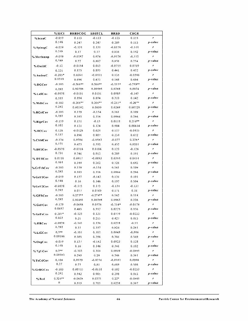
%Si/Cl

%Scene -0.059 0.548

% SpirogC -0.059 0.548

%Merismop -0.059 0.548

% OscillC -0.12

0.221

%AudouC -0.205* 0.0349

%DGCov -0.103

0.292

%LsSCov -0.0838

%MdbCov

%BGs1Cov

%B1grCov

%BCCov

%Cb1dCov

%DFi!Cov

% DTBCov

%GrFtbCov

%GrF1Cov

%GrF2Cov

%GFBCov

%GrFCov

%GrFsCov

%HBCov

%LIGCov

%0rgCov

0.393

-0.103

0.292

-0.103

0.292

-0.159

0.102

0.138

0.157

-0.134

0.171

-0.0338

0.731

0.0718

0.464

-0.103

0.292

-0.059

0.548

-0.0838

0.393

-0.103

0.292

-0.179

0.0657

0.207*

0.033

-0.0838

0.392

0.3**

0.00186

-0.059

0.548

% TgLCov 0.3** 0.00183

%TsCdCov 0.108 0.27

I%GrBGCov -0.103

0.292 I I %Bed

I 0.324**

0

BRBDCOG SDSTCL

0.113 -0.113

0.247 0.247

-0.134 0.134

0.17 0.17

-0.0287 0.024

0.77 0.807

-0.0154 0.013

0.875 0.895

0.0384 -0.0411

0.696 0.675

-0.26 6** 0. 26 6**

0.00598 0.00595

-0.0131 0.0131

0.894

-0.26 6**

0.00592

0.159

0.103

0.151

0.121

-0.0128

0.896

0.0704

0.473

-0.0318

0.746

0.0917

0.349

0.159

0.103

0.137

0.16

-0.173

0.077

0.273**

0.00481

-0.0688

0.483

-0.123

0.21

-0.141

0.15

-0.101

0.303

0.137

0.16

-0.103

0.295

0.0339

0.73

0.00715

0.942

-0.0638

0.515

0.894

0.26 6**

0.0059

-0.154

0.116

-0.15

0.124

0.024

0.807

-0.0583

0.552

0.0108

0.912

-0.0893

0.362

-0.154

0.116

-0.142

0.146

0.173

0.0769

-0.27 8**

0.00398

0.0576

0.557

0.121

0.215

0.138

0.157

0.102

0.298

-0.142

0.146

0.104

0.29

-0.0236

0.81

-0.0118

0.905

0.0371

0.705


BRBD

-0.123

0.209

-0.0178

0.856

-0.0178

0.856

-0.0755

0.441

0.135

0.168

-0.215*

0.0269

0.0989

0.313

-0.215*

0.0269

0.161

0.0984

0.0118

0.904

0.117

0.234

-0.077

0.432

0.123

0.209

0.0344

0.726

0.161

0.0984

0.126

0.197

-0.134

0.171

0.162

0.0963

-0.214*

0.0275

0.0779

0.427

0.0218

0.824

0.0849

0.386

0.0923

0.346

0.0849

0.386

-0.0392

0.689

0.102

0.298

0.22*

0.0238

66

CBGR

0.155

0.113

-0.144

0.142

-0.112

0.254

0.0769

0.432

-0.0396

0.686

-0.25 9**

0.0074

-0.143

0.142

-0.26 **

0.00729

0.109

0.266

0.25 6**

0.00814

-0.0415

0.672

0.226*

0.0201

-0.128

0.191

0.0454

0.643

0.109

0.266

0.101

0.304

-0.137

0.16

0.118

0.226

-0.0178

0.856

-0.0232

0.813

-0.11

0.261

-0.088

0.369

0.128

0.192

-0.0895

0.361

0.0998

0.308

-0.0233

0.813

-0.0885

0.367

r

p-va1ue

r

p-va1ue

r

p-va1ue

r

p-va1ue

r

p-va1ue

r

p-va1ue

r

p-va1ue

r

p-va1ue

r

p-va1ue

r

p-va1ue

r

p-va1ue

r

p-va1ue

r

p-va1ue

r

p-va1ue

r

p-value

r

p-value

r

p-value

r

p-value

r

p-value

r

p-value

r

p-value

r

p-value

r

p-value

r

p-value

r

p-value

r

p-value

r

p-value


%Si/Cl BRBDCOG SDSTCL BRBD CBGR

%Bo -0.19 0.42 ** -0.42 2** 0.983** -0.0829 r

0.0512 0 0 0 0.398 p-va1ue

%Cob -0.26 9** 0.67 7** -0.66 9** 0.27 8** 0.641 ** r

0.00534 0 0 0.00396 0 p-va1ue

%Gra 0.0801 0.407** -0.384** -0.3** 0.66 ** r

0.414 0 0 0.00184 0 p-va1ue

%8 -0.00147 -0.87 8** 0. 89 2** -0.32 8** -0.603** r

0.988 0 0 0 0 p-va1ue

%Si/Cl -0.28 6** 0.29 9** -0.137 -0.0783 r

0.00307 0.0019 0.161 0.424 p-va1ue

BRBDCOG -0.98 6** 0.407** 0.674** r

0 0 0 p-va1ue

SDSTCL -0.41 7** -0.65 6** r

0 0 p-va1ue

BRBD -0.102 r

0.295 p-va1ue

CBGR r

Tbe Academy of Nat ural Sciences 67 Patrick Center for Environmenta!Researcb

Appendix 4: Results of Forward stepwise regression for dependent variables Chi a and AFDM. Abbreviations used for variables are the same as listed under Notes in Appendix 3.

a) Forward Stepwise Regression: Dependent Variable: chl_a F-to-Enter: 4.000 P = 0.048 F-to-Remove: 3.900 P = 0.051

Step 0: Standard Error of Estimate= 0.380

Analysis of Variance: Group DF ss MS F p

Residual 105 15.130 0.144

Variables in Model Group Coef. Std. Coeff. Std. Error F-to-Remove p

Constant 1.879 0.0369

Variables not in Model Group F-to-Enter p

NH3-N 0.275 0.601 P04 7.278 0.008 TP 5.272 0.024 N03-N 9.949 0.002 DO 0.00381 0.951 pH 1.534 0.218 COND 3.718 0.057 B size 31.019 <0.001 %0 30.218 <0.001 %Bed 0.0771 0.782 %Bo 0.0157 0.901 %Cob 3.969 0.049 %Gra 6.569 0.012 %S 1.716 0.193 %Si/Cl 4.349 0.039 BBDCOGR 7.793 0.006 SDSTCL 5.617 0.020 BRBD 0.00291 0.957 CBGR 6.045 0.016 R wid 19.025 <0.001 R len 13.716 <0.001 Flow 0.298 0.587

Step 1: BASIN Entered R = 0.479 Rsqr = 0.230 Adj Rsqr = 0.222 Standard Error of Estimate= 0.335


Regression 3.476 3.476 31.019 <0.001 Residual 104 11.654 0.112



Constant 1.259 0.116 B size 0.421 0.479 0.0756 31.019 <0.001

Variables not in Model Group F-to-Enter p NH3-N 0.113 0.738 P04 1.418 0.236 TP 0.941 0.334 N03-N 9.104 0.003 DO 0.951 0.332 pH 0.351 0.555 COND 3.643 0.059 %0 0.245 0.622 %Bed 0.00813 0.928 %Bo 0.292 0.590 %Cob 3.126 0.080 %Gra 3.266 0.074 %S 0.517 0.474 %Si/Cl 5.433 0.022 BRBDCOGR 6.164 O.ol5 SDSTCL 3.127 0.080 BRBD 0.275 0.601 CBGR 4.119 0.045 R wid 1.014 0.316 R len 0.900 0.345 Flow 0.0631 0.802

Step 2: N03-N Entered R = 0.541 Rsqr = 0.292 Adj Rsqr = 0.279 Standard Error of Estimate= 0.322

Analysis of Variance: Group DF ss MS F p Regression 2 4.423 2.211 21.270 <0.001 Residual 103 10.708 0.104


Constant 0.407 0.304 N03-N 0.285 0.251 0.0943 9.104 0.003 B size 0.400 0.455 0.0732 29.833 <0.001

Variables not in Model Group F-to-Enter p NH3-N 0.445 0.506 P04 0.0309 0.861 TP 0.115 0.735 DO 0.344 0.559 pH 3.190 0.077 COND 1.712 0.194


%0 0.765 0.384 %Bed 0.636 0.427 %Bo 1.348 0.248 %Cob 6.115 O.ol5 %Gra 2.012 0.159 %S 1.563 0.214 %Si/Cl 6.686 0.011 BRBDCOGR10.180 0.002 SDSTCL 5.350 0.023 BRBD 0.942 0.334 CBGR 4.708 0.032 R wid 0.539 0.465 R len 0.197 0.658 Flow 0.135 0.714

Step 3: BRBDCOGR Entered R = 0.597 Rsqr = 0.357 Adj Rsqr = 0.338 Standard Error of Estimate= 0.309


Regression 3 5.394 1.798 18.837 <0.001 Residual 102 9.736 0.0955


Constant -0.156 0.340 N03-N 0.333 0.294 0.0917 13.201 <0.001 B size 0.369 0.420 0.0708 27.187 <0.001 BRBDCOGR0.0566 0.259 0.0177 10.180 0.002


NH3-N 0.0289 0.865 P04 1.144 0.287 TP 0.720 0.398 DO 1.460 0.230 pH 0.672 0.414 COND 1.251 0.266 %0 0.455 0.501 %Bed 1.365 0.245

%Bo 0.0409 0.840 %Cob 0.00237 0.961 %Gra 0.274 0.602 %S 2.654 0.106 %Si/Cl 2.690 0.104 SDSTCL 1.172 0.282 BRBD 0.185 0.668 CBGR 0.852 0.358 R wid 0.0434 0.835 R len 0.0343 0.854 Flow 0.682 0.411


Summary Table Step# Vars. Entered V ars. Removed R RSqr Delta RSqr V ars in Model 1 B size 0.479 0.230 0.230 1 2 N03-N 0.541 0.292 0.0626 2 3 BRBDCOGR 0.597 0.357 0.0642 3

The dependent variable chl_a can be predicted from a linear combination of the independent variables: p

N03-N B size BRBDCOGR

<0.001 <0.001

0.002

J'he followin_g variables did not significantly add to the ability of the equation to predict chl_a and were not mcluded m tfie tmal equatwn:

t;\~.a;N P04 TP DO pH COND %0 %Bed %Bo %Cob %Gra %S %Si/Cl SDSTCL BRBD CBGR R_wid R_len

Normality Test: Passed (P = 0.657) Constant Variance Test: Passed (P = 1.000) Power of performed test with alpha= 0.050: 1.000


Appendix 4

b) Forward Stepwise Regression: Dependent Variable: AFDM F-to-Enter: 4.000 P = 0.048 F-to-Remove: 3.900 P = 0.051

Step 0: Standard Error of Estimate= 0.332

Analysis of Variance: Group DF ss MS Residual 105 11.561 0.110

Variables in Model Group Coef. Std. Coeff. Constant 1.165


NH3-N 1.382 0.242 P04 1.970 0.163 TP 2.534 0.114 N03-N 18.620 <0.001 DO 1.155 0.285 pH 3.669 0.058 COND 0.00651 0.936 B size 6.616 0.012 %0 5.824 O.ol8 %Bed 0.263 0.609 %Bo 3.708 0.057 %Cob 0.824 0.366 %Gra 1.132 0.290 %S 0.804 0.372 %Si/Cl 0.00152 0.969 BRBDCOGR 0.540 0.464 SDSTCL 0.591 0.444 BRBD 3.357 0.070 CBGR 0.0408 0.840 R wid 5.040 0.027 R_leng 4.552 0.035 Flow 0.734 0.394

Step 1: N03-N Entered

F p

Std. Error 0.0322

F-to-Remove

R = 0.390 Rsqr = 0.152 Adj Rsqr = 0.144 Standard Error of Estimate= 0.307

Analysis of Variance: Group DF Regression Residual 104

ss 1.755 9.805


MS 1.755 0.0943

F 18.620

72

p <0.001

p


Variables in Model Group Coef. Std. Coeff. Std. Error Constant -0.0332 0.279 N03-N 0.386 0.390 0.0894

Variables not in Model Group F-to-Enter p NH3-N 0.00181 0.966 P04 0.312 0.578 TP 0.0512 0.821 DO 0.408 0.524 pH 0.453 0.502 COND 0.874 0.352 B size 5.519 0.021 %0 5.404 0.022 %Bed 0.432 0.513 %Bo 1.526 0.220 %Cob 0.0545 0.816 %Gra 0.184 0.669 %S 0.122 0.727 %Si/Cl 0.0253 0.874 BRBDCOGR 0.0198 0.888 SDSTCL 0.0923 0.762 BRBD 1.834 0.179 CBGR 0.0577 0.811 R wid 3.259 0.074 R len 2.035 0.157 Flow 0.0139 0.906

Step 2: BASIN Entered R = 0.442 Rsqr = 0.195 Adj Rsqr = 0.179 Standard Error ofEstimate = 0.301

Analysis of Variance: Group DF Regression 2 Residual 103

Variables in Model Group Coef. Constant -0.207 N03-N 0.366 B size 0.160

Variables not in Model Group F-to-Enter NH3-N 0.203 P04 2.024 TP 0.851

DO 1.315 pH 1.336 COND 1.045

ss 2.254 9.307

MS 1.127 0.0904

Std. Coeff.

0.369 0.209

p

0.653 0.158 0.358

0.254 0.250 0.309


F 12.474

Std. Error 0.283 0.0879 0.0682

73

F-to-Remove

18.620

p <0.001

F-to-Remove

17.295 5.519

p

<0.001

p

<0.001 0.021


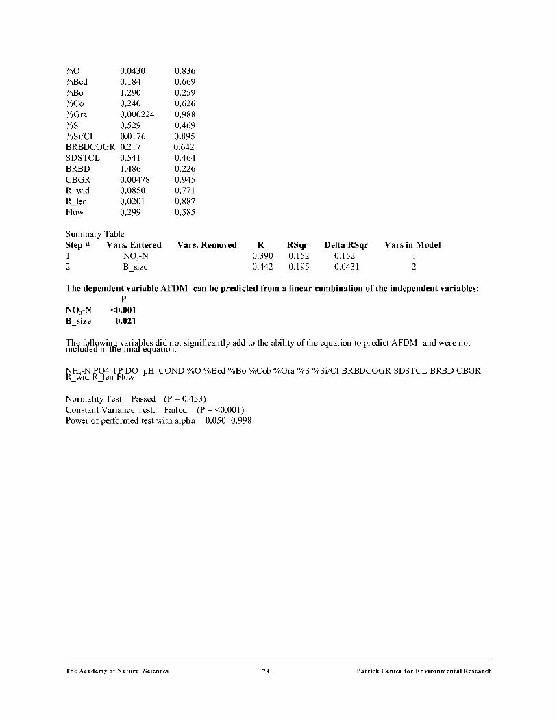
%0 0.0430 %Bed 0.184 %Bo 1.290 %Co 0.240 %Gra 0.000224 %S 0.529 %Si/Cl 0.0176 BRBDCOGR 0.217 SDSTCL 0.541 BRBD 1.486 CBGR 0.00478 R wid 0.0850 R len 0.0201 Flow 0.299

Summary Table Step# Vars. Entered 1 N03-N 2 B size

0.836 0.669 0.259 0.626 0.988 0.469 0.895 0.642 0.464 0.226 0.945 0.771 0.887 0.585

V ars. Removed R 0.390 0.442

RSqr 0.152 0.195

Delta RSqr 0.152 0.0431

V ars in Model 1 2

The dependent variable AFDM can be predicted from a linear combination of the independent variables: p

<0.001 0.021

J'he followin_g variables did not significantly add to the ability of the equation to predict AFDM and were not mcluded m tne tmal equatwn:

NH3-N P04 TP DO pH COND %0 %Bed %Bo %Cob %Gra %S %Si/Cl BRBDCOGR SDSTCL BRBD CBGR R wid R len Flow - -

Normality Test: Passed (P = 0.453) Constant Variance Test: Failed (P = <0.001) Power of performed test with alpha= 0.050: 0.998


Documents

Understanding the Relationship Between Natural Conditions