Embed Size (px)
Citation preview
Understanding the Role of Adolescent Social Networks
and Neighborhood Peer Effects on Obesogenic Behaviors
and Weight Outcomes using Spatial Analysis Author: Olugbenga Ajilore
Affiliation: University of Toledo
E-mail: [email protected]
JEL Classification: A14, C21, D85, R12
Keywords: Obesity, Social networks, Neighborhood Effects, Spatial Econometrics
ABSTRACT There is an ongoing debate as to the degree to which an adolescent’s peer group affects whether they engage in activity that leads to obesity. This paper moves beyond the standard peer effects literature by using spatial econometrics to answer questions on how peers influence adolescent obesity. There have been significant advances in the use of spatial econometrics to estimate peer effects. There are a variety of models that can solve the well-known “reflection problem” that plagues the peer effects literature. This paper furthers the literature by looking at the community contexts of peer effects as well as the school contexts. I specify alternative spatial weight matrices to account for peer effects in the school environment and peer effects in the neighborhood environment. I use data from the National Longitudinal Study on Adolescent Health Survey to answer these questions since it provides the data necessary to estimate spatial models. This is an important study since neighborhood effects can either enhance or detract from school-based policies to combat obesity among youth.
1 | P a g e
1 INTRODUCTION
Childhood obesity is a serious problem that plagues American youth. Data shows that the
percentage of children ages 12 to 19 who are considered obese has increased from 5% in 1980 to
18% in 2010 (Ogden et al, 2012). Obesity in youth can lead to short-run as well as long-run
adverse health effects. These adolescents are also subject to social and psychological problems
stemming from their weight issues (Crosnoe et al, 2008). This problem has been the subject of
much study and scholars have found many reasons for the increases in childhood obesity.
Papoutsi et al (2012) find three major factors that can explain the rise in childhood obesity: the
environment created by parental work intensity, diet, and food advertising. Larson et al (2013)
find that the influence of multiple contexts, including family, peer, and neighborhood contexts,
impact childhood obesity.
Recently, the focus of study on childhood obesity has been on the role of peers and their
influence of obesity and obesity-related behaviors. Recent studies show that the one’s peers have
a large impact on obesity (Cunningham et al, 2012). The study of peer effects in health behaviors
has flourished because of the realization while individuals make choices based on individual
preferences, their decisions can be influenced by others (Blume et al, 2010). While the analysis
of peer influence on obesity is well researched, there are noted methodological issues with the
estimation of peer effects (Manski, 1993). Many studies on peer effects do not account for these
issues and in the studies that try to correct for these issues, most scholars use either school fixed
effects or instrumental variable regression techniques to model the endogenous interactions
(Fletcher, 2011).
Recent advances in spatial econometrics using social networks have been shown to be an
improvement on identification (Lee, Liu, and Lin, 2010). Several authors have used spatial
2 | P a g e
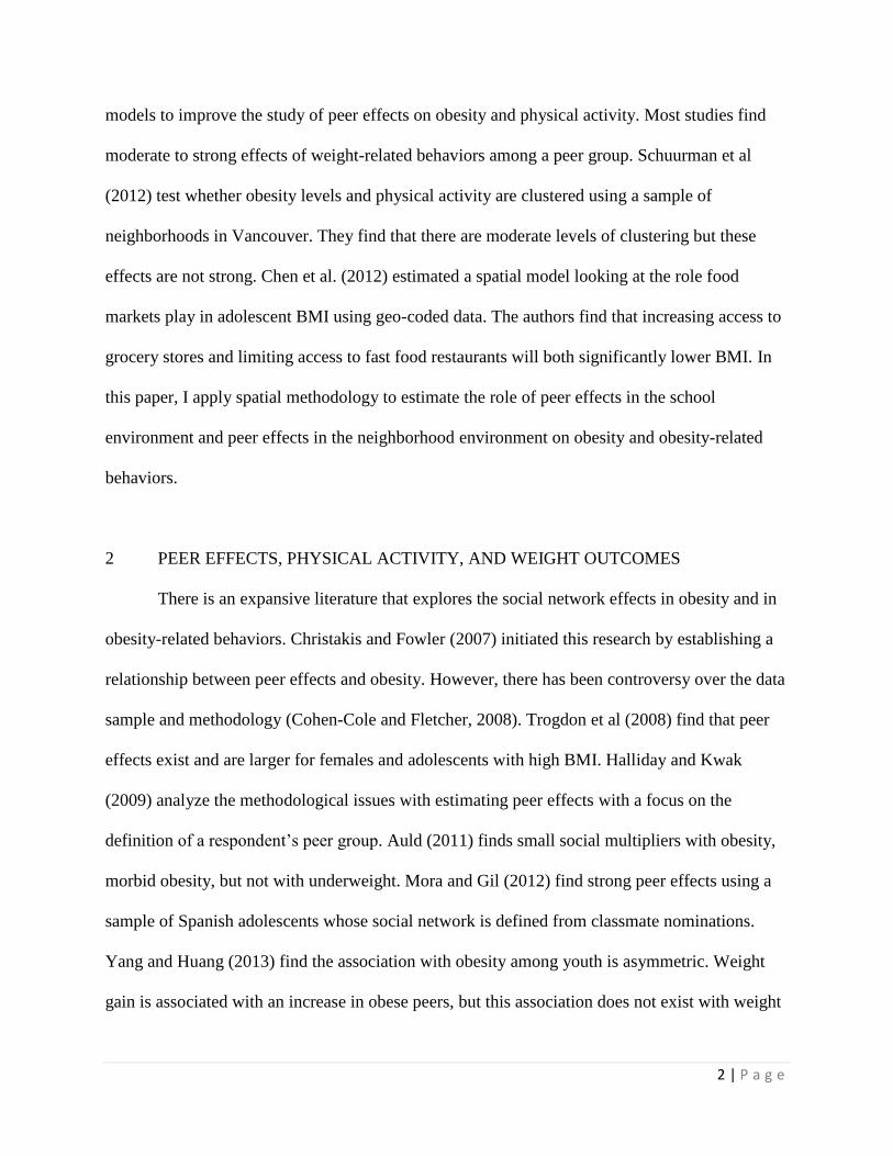
models to improve the study of peer effects on obesity and physical activity. Most studies find
moderate to strong effects of weight-related behaviors among a peer group. Schuurman et al
(2012) test whether obesity levels and physical activity are clustered using a sample of
neighborhoods in Vancouver. They find that there are moderate levels of clustering but these
effects are not strong. Chen et al. (2012) estimated a spatial model looking at the role food
markets play in adolescent BMI using geo-coded data. The authors find that increasing access to
grocery stores and limiting access to fast food restaurants will both significantly lower BMI. In
this paper, I apply spatial methodology to estimate the role of peer effects in the school
environment and peer effects in the neighborhood environment on obesity and obesity-related
behaviors.
2 PEER EFFECTS, PHYSICAL ACTIVITY, AND WEIGHT OUTCOMES
There is an expansive literature that explores the social network effects in obesity and in
obesity-related behaviors. Christakis and Fowler (2007) initiated this research by establishing a
relationship between peer effects and obesity. However, there has been controversy over the data
sample and methodology (Cohen-Cole and Fletcher, 2008). Trogdon et al (2008) find that peer
effects exist and are larger for females and adolescents with high BMI. Halliday and Kwak
(2009) analyze the methodological issues with estimating peer effects with a focus on the
definition of a respondent’s peer group. Auld (2011) finds small social multipliers with obesity,
morbid obesity, but not with underweight. Mora and Gil (2012) find strong peer effects using a
sample of Spanish adolescents whose social network is defined from classmate nominations.
Yang and Huang (2013) find the association with obesity among youth is asymmetric. Weight
gain is associated with an increase in obese peers, but this association does not exist with weight
3 | P a g e
loss. There is a general consensus that peer effects do play a role in obesity, but the mechanisms
by which they influence obesity need better understanding.
Many researchers have estimated the role that peer effects play in the link between
physical activity and weight. Peer effects have been found at all ages from children to college
age individuals. Ali et al (2011) find that that peer effects play a role in physical activity, which
has implications for adolescent obesity. Carrell et al (2011) find that college peers who had poor
fitness levels influence others. Gesell et al (2012) find that increasing activity levels in an
afterschool program can boost the activity levels of a child through their immediate social
network. Fitzgerald et al (2012) review of adolescent physical activity and their peers. De la
Haye et al (2010) find gender based similarities in obesogenic behaviors. Female friends are
more likely to engage in screen-time activities while male friends engage in high calorie food
consumption. De la Haye et al (2011) find that friends to not only engage in similar behavior but
also tend to choose friends based on similar levels of physical activities. This literature shows
that interventions geared towards weight-reducing behavior can spread in individual’s peer
group.
While a major focus of the peer effects literature is on an adolescent’s social network,
neighborhoods can play a role in individual behavior. Diez-Roux and Mair (2010) explore the
role of residential environments on various health outcomes and health inequities. The structural
conditions of neighborhoods can play a role in the development of attitudes and norms that can
influence the behavior of individuals within those neighborhoods (Galster, 2012). Research on
neighborhood effects and obesity focus on the built environment and how home location affect
obesity. Neighborhood effects could pick up the fact that people in a community can encourage
or discourage positive obesity reducing behavior. Cohen et al (2006) show that increased
4 | P a g e
neighborhood collective efficacy can reduce the probability of obesity risk and overweight.
Neighborhood effects can influence weight-related behaviors through a variety of geographic
mechanisms (Li et al, 2009; Lopez, 2007; Nelson et al, 2006). However, the study of
neighborhood peer effects has not taken advantage of the framework used in social network
studies to understand the role of peer effects and obesity. In this paper, I look at the both types of
peer effects using a social interactions framework to compare and contrast the different effects of
peers on obesity and obesity related behavior.
3 SOCIAL INTERACTION MODELS
Social interaction models study the relationship between interactions among individuals
and collective behavior. These models can help explain the observation that individuals within
the same group tend to exhibit the same behavior. Akerlof (1997) emphasized the importance of
group behavior as a primary driver of individual’s choices: “As a consequence, the impact of my
choices on my interactions with other members of my social network may be the primary
determinant of my decision, with the ordinary determinants of choice of only secondary
importance.” Social interaction models can be used to identify peer group effects from the data.
Peer groups can influence adolescent decision-making through three mechanisms: endogenous
interactions, contextual interactions, and correlated effects (Manski, 2000). Endogenous
interactions occur when the behavior of the group affects the behavior of the individual,
contextual interactions occur when characteristics of the group like age, gender, or race affect the
behavior of the individual, and correlated effects occur when the environment plays a role in the
behavior of individuals within a group. Several authors have sought to empirically test these
interactions and effects, mostly the endogenous interactions (Blume and Durlauf, 2005).
5 | P a g e
A problem with the estimation of social interaction models is the “reflection” problem
(Manski, 1993). While peers’ outcome affects the individual’s decision, the individual’s decision
could influence the peers’ outcome. In the reduced form of the social interaction framework, the
endogenous interactions and the contextual interactions cannot be separated (Durlauf and
Ioannides, 2010). The key question in the literature has been how to disentangle these
interactions and properly identify the model. The application of spatial econometrics using social
networks has been shown to be an improvement on identification (Bramoulle, Djebbari, and
Fortin, 2009; Lee, 2007; Lee, Liu, and Lin, 2010). Blume et al (2010) argue, “Social network
models provide further focus on the microstructure of interactions among agents and allow for
heterogeneity of interactions across pairs of agents.” Instead of using peers’ means, we are able
to explicitly model the interactions between members of the same group. Lin (2010) argues that
the spatial autoregressive (SAR) model provides enough information to identify the endogenous
and contextual interactions, thus avoiding the reflection problem.
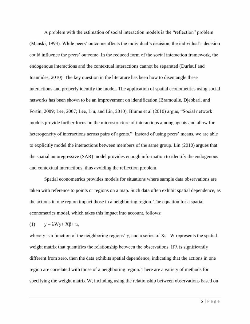
Spatial econometrics provides models for situations where sample data observations are
taken with reference to points or regions on a map. Such data often exhibit spatial dependence, as
the actions in one region impact those in a neighboring region. The equation for a spatial
econometrics model, which takes this impact into account, follows:
(1) y = λWy+ Xβ+ u,
where y is a function of the neighboring regions’ y, and a series of Xs. W represents the spatial
weight matrix that quantifies the relationship between the observations. If λ is significantly
different from zero, then the data exhibits spatial dependence, indicating that the actions in one
region are correlated with those of a neighboring region. There are a variety of methods for
specifying the weight matrix W, including using the relationship between observations based on
6 | P a g e
Euclidean distances (a nearest-neighbors matrix) or assigning values of 1 if regions are adjacent
and 0 otherwise (first-order contiguity matrix).
In the social interactions literature, W represents a social network weight matrix where
individuals are assigned a 1 if they are in the same peer group and a 0 otherwise. The
endogenous peer effect is represented by λ in (1). To fully incorporate all the mechanisms in a
social interactions model we outline a generalized version of the Cliff-Ord spatial model that
allows for spatial interactions in the dependent variable, explanatory variables, and the
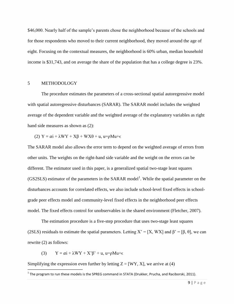
disturbances. The empirical specification is given in (2):
(2) Y = 𝛼i + λWY + Xβ + WXθ + u, u=ρMu+ϵ
In the social interactions framework, the first term (λWy) is the endogenous interaction, the
spatially lagged explanatory variables (WXθ) are the contextual interactions, and the spatial
interactions in the disturbances (ρMu) are the correlated effects. While the group fixed effects
(𝛼i) represent common environmental factors, there may be correlated effects beyond these
factors. The spatial interactions on the disturbance also controls for network formation. A
positive coefficient denotes that the group forms over similar behavior and a negative coefficient
denotes the group does not form over similar behavior. W and M are the weight matrices that
specify the relationship between units. In the next section, we describe the data that allows us to
estimate the spatial model.
4 DATA
The data is taken from the National Longitudinal Study on Adolescent Health (Add
Health). Beginning with an in-school questionnaire administered to a nationally representative
sample of students in grades 7 through 12 in 1994-95, the study follows up with a series of in-
7 | P a g e
home interviews of respondents in subsequent years. A unique feature of Add Health is that the
first wave contains information on individuals’ nominations of their closest friends. Since these
friends were also surveyed, this allows us to craft weight matrices based off of this friendship
network. The data is taken from the in-home survey of Wave 1. The number of observations in
the sample is 12,398.
There are several dependent variables chosen to represent behavior that influences
obesity that have been used in the literature (Rees and Sabia, 2010; Ali et al, 2011). The first
dependent variable measures the number of times per week the respondent engaged in exercise,
sport, or physical activities like rollerblading and biking. This measure is a continuous variable
that aggregates the number of times per week the respondent engaged in rollerblading or roller
skating, played an active sport like basketball or baseball, and exercised. The next set of
dependent variables indicate how many days during the week the individual engages in physical
activities and how many days during the week the individual engage in screen-time activities.
We also measure the number of hours the respondent watches television or plays video games.
The explanatory variables include basic demographics like age, grade, gender, race and
ethnic status. Also included is if the respondent was born in the United States, if they are the first
born, the number of siblings, age when they moved to their current home, if they were taught
about weight issues in school, and their test score on the Peabody Picture Vocabulary Test
(PVT). We include characteristics of the parents like whether they are college educated, whether
work full time, their pre-tax income, and if they chose the neighborhood because of the schools.
The price of groceries and the price of junk food are included. Contextual data about the
community are included like the percent of the block that is urban, median household income,
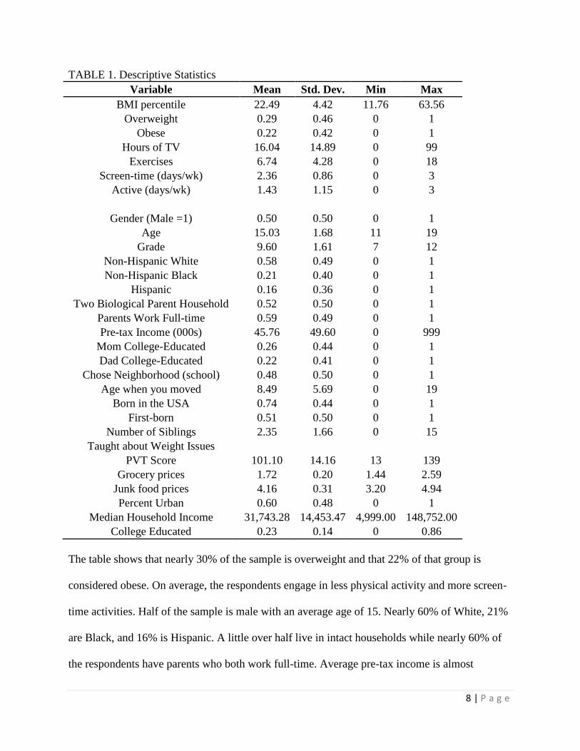
and the percentage that have college degrees. Table 1 gives a summary of the variables.
8 | P a g e
TABLE 1. Descriptive Statistics
Variable Mean Std. Dev. Min Max
BMI percentile 22.49 4.42 11.76 63.56
Overweight 0.29 0.46 0 1
Obese 0.22 0.42 0 1
Hours of TV 16.04 14.89 0 99
Exercises 6.74 4.28 0 18
Screen-time (days/wk) 2.36 0.86 0 3
Active (days/wk) 1.43 1.15 0 3
Gender (Male =1) 0.50 0.50 0 1
Age 15.03 1.68 11 19
Grade 9.60 1.61 7 12
Non-Hispanic White 0.58 0.49 0 1
Non-Hispanic Black 0.21 0.40 0 1
Hispanic 0.16 0.36 0 1
Two Biological Parent Household 0.52 0.50 0 1
Parents Work Full-time 0.59 0.49 0 1
Pre-tax Income (000s) 45.76 49.60 0 999
Mom College-Educated 0.26 0.44 0 1
Dad College-Educated 0.22 0.41 0 1
Chose Neighborhood (school) 0.48 0.50 0 1
Age when you moved 8.49 5.69 0 19
Born in the USA 0.74 0.44 0 1
First-born 0.51 0.50 0 1
Number of Siblings 2.35 1.66 0 15
Taught about Weight Issues
PVT Score 101.10 14.16 13 139
Grocery prices 1.72 0.20 1.44 2.59
Junk food prices 4.16 0.31 3.20 4.94
Percent Urban 0.60 0.48 0 1
Median Household Income 31,743.28 14,453.47 4,999.00 148,752.00
College Educated 0.23 0.14 0 0.86
The table shows that nearly 30% of the sample is overweight and that 22% of that group is
considered obese. On average, the respondents engage in less physical activity and more screen-
time activities. Half of the sample is male with an average age of 15. Nearly 60% of White, 21%
are Black, and 16% is Hispanic. A little over half live in intact households while nearly 60% of
the respondents have parents who both work full-time. Average pre-tax income is almost
9 | P a g e
$46,000. Nearly half of the sample’s parents chose the neighborhood because of the schools and
for those respondents who moved to their current neighborhood, they moved around the age of
eight. Focusing on the contextual measures, the neighborhood is 60% urban, median household
income is $31,743, and on average the share of the population that has a college degree is 23%.
5 METHODOLOGY
The procedure estimates the parameters of a cross-sectional spatial autoregressive model
with spatial autoregressive disturbances (SARAR). The SARAR model includes the weighted
average of the dependent variable and the weighted average of the explanatory variables as right
hand side measures as shown as (2):
(2) Y = 𝛼i + λWY + Xβ + WXθ + u, u=ρMu+ϵ
The SARAR model also allows the error term to depend on the weighted average of errors from
other units. The weights on the right-hand side variable and the weight on the errors can be
different. The estimator used in this paper, is a generalized spatial two-stage least squares
(GS2SLS) estimator of the parameters in the SARAR model1. While the spatial parameter on the
disturbances accounts for correlated effects, we also include school-level fixed effects in school-
grade peer effects model and community-level fixed effects in the neighborhood peer effects
model. The fixed effects control for unobservables in the shared environment (Fletcher, 2007).
The estimation procedure is a five-step procedure that uses two-stage least squares
(2SLS) residuals to estimate the spatial parameters. Letting X’ = [X, WX] and β’ = [β, θ], we can
rewrite (2) as follows:
(3) Y = 𝛼i + λWY + X’β’ + u, u=ρMu+ϵ
Simplifying the expression even further by letting Z = [WY, X], we arrive at (4) 1 The program to run these models is the SPREG command in STATA (Drukker, Prucha, and Raciborski, 2011).

10 | P a g e
(4) Y=Zδ + u, u=ρMu+ϵ
Step one in the procedure estimates δ by 2SLS using an instrument matrix H comprised of
linearly independent columns (X, WX, W2X, …, W
qX, MX, M
2X, …,, M
qX). Step two provides
an initial GMM estimator of ρ based on 2SLS residuals. This initial estimator is consistent but
not efficient, so in step three an efficient GMM estimator of ρ using a weight nonlinear least
squares estimator, again based on 2SLS residuals. The G2SSLS estimator of δ is the 2SLS
estimator of the transformed model, where we pre-multiply (4) by I – ρM, with Y* = Y – ρMY
and Z* = Z – ρMZ, and replacing ρ with the ρ calculated from step three. The final step is to get
the efficient GMM estimator of ρ based on GS2SLS results.
6 FINDINGS
There are two peer groups used in the specification of the weight matrices. The first
matrix comprises of individuals who are in the same grade at the same school (school-grade).
The second weight matrix comprises of individuals who live within a similar distance from the
school (neighborhood). I create a 10 nearest neighbor matrix, where the peer receives a 1 if they
are one of the ten nearest neighbors to the respondent. Table 2 provides the results of the
GS2SLS estimation of both school-grade peer effects and neighborhood peer effects on obesity
and obesity status. The table reports the coefficients on the spatial parameters2.
Table 2. GS2SLS Estimation of Peer Effects on Obesity and Obesity Status
Peer Group Spatial Parameter BMI Percentile Overweight Obese
School-Grade λ -0.9677*** -1.0534*** -0.7114***
ρ 0.4417*** 0.4556*** 0.5357***
Neighborhood λ 0.7282*** 0.8133*** 0.9400***
ρ -0.5287*** -0.5083*** -0.7667***
*** - sig. at 1% level; ** - sig. at 5% level
2 Full results are available upon request.

11 | P a g e
The results from Table 2 show that the endogenous peer effect is different depending on the peer
group definition. The BMI of individuals are negatively affected by the BMI of school-grade
peers, while an individual’s BMI is positively affected by the BMI of neighborhood peers.
Spatial parameter on errors is significant and positive in the school-grade model, but it is
significant and negative in the neighborhood model. This signifies that an exogenous shock to
one individual will cause moderate changes in the BMI in those in the peer groups.
The next analysis focuses on the role of peer effects on physical activity like sports and
exercise and on sedentary activities like watching television or videos. Table 3 provides the
results of school-grade peers on physical activity and sedentary activity.
Table 3. GS2SLS Estimation of Peer Effects on Obesogenic Behaviors
Peer Group Spatial Parameter Exercise Active Screen-time Hours of TV
School-Grade λ -1.1473*** -1.1427*** -0.7999*** -1.0330***
ρ 0.5483*** 0.5845*** 0.3493*** 0.4864***
Neighborhood λ 0.8354*** 0.8043*** 0.8625*** 0.8157***
ρ -0.6010*** -0.6804*** -0.6253*** -0.5818***
*** - sig. at 1% level; ** - sig. at 5% level
The results are similar to Table 2 where the endogenous peer effect is negative for school-grade
peers and positive for neighborhood peers, while the spatial parameter on the disturbances is
positive for school-grade peers and negative for neighborhood peers.
7 CONCLUSION
This paper is the first to compare peer effects within the school environment with peer
effects in the neighborhood using a spatial approach. The spatial approach to modeling peer
effects has become popular over the last few years with the application of spatial econometric
12 | P a g e
models to networks (see Bramoulle, Djebbari, and Fortin (2009), Lee (2007), Lee, Liu, and Lin
(2010)). Currently, this approach has been used to study peer effects in education (Calvo-
Armengol et al, 2009) and peer effects in crime (Patacchini and Zenou, 2012). This approach has
yet to be applied to the study of peer effects and obesity-related behaviors. This paper showed
that peer effects exist with obesity-related behaviors.
13 | P a g e
REFERENCES
Akerlof, George A. "Social distance and social decisions." Econometrica: Journal of the
Econometric Society (1997): 1005-1027.
Ali, Mir M., Aliaksandr Amialchuk, and Frank W. Heiland. "Weight-related behavior among
adolescents: the role of peer effects." PloS one 6.6 (2011): e21179.
Anselin, Luc. Spatial econometrics: methods and models. Vol. 4. Springer, 1988.
Arraiz, Irani, David M. Drukker, Harry H. Kelejian, and Ingmar R. Prucha. "A SPATIAL
CLIFF‐ORD‐TYPE MODEL WITH HETEROSKEDASTIC INNOVATIONS: SMALL AND
LARGE SAMPLE RESULTS*." Journal of Regional Science 50, no. 2 (2009): 592-614.
Auld, M. Christopher. "Effect of large-scale social interactions on body weight."Journal of
Health Economics 30.2 (2011): 303-316.
Blume, Lawrence E., and Steven N. Durlauf. Identifying social interactions: A review. Social
Systems Research Institute, University of Wisconsin, 2005.
Blume, Lawrence E., William A. Brock, Steven N. Durlauf, and Yannis Ioannides.
"Identification of social interactions." (2010).
Bramoullé, Yann, Habiba Djebbari, and Bernard Fortin. "Identification of peer effects through
social networks." Journal of econometrics 150.1 (2009): 41-55.
Calvó-Armengol, Antoni, Eleonora Patacchini, and Yves Zenou. "Peer effects and social
networks in education." The Review of Economic Studies 76.4 (2009): 1239-1267.
Carrell, Scott E., Mark Hoekstra, and James E. West. "Is poor fitness contagious?: Evidence
from randomly assigned friends." Journal of Public Economics 95.7 (2011): 657-663.
Chen, S. E., Florax, R. J., & Snyder, S. D. (2012). Obesity and fast food in urban markets: a new
approach using geo‐referenced micro data. Health Economics
Christakis, Nicholas A., and James H. Fowler. "The spread of obesity in a large social network
over 32 years." New England journal of medicine 357.4 (2007): 370-379.
Cohen, Deborah A., et al. "Collective efficacy and obesity: the potential influence of social
factors on health." Social Science & Medicine 62.3 (2006): 769-778.
Cohen-Cole, Ethan, and Jason M. Fletcher. "Detecting implausible social network effects in
acne, height, and headaches: longitudinal analysis." BMJ: British Medical Journal 337 (2008).
Crosnoe, R., Frank, K., & Mueller, A. S. (2008). Gender, body size and social relations in
American high schools. Social Forces, 86(3), 1189-1216.
14 | P a g e
Cunningham, S. A., Vaquera, E., Maturo, C. C., & Venkat Narayan, K. M. (2012). Is there
evidence that friends influence body weight? A systematic review of empirical research. Social
Science & Medicine
De La Haye, Kayla, et al. "Homophily and contagion as explanations for weight similarities
among adolescent friends." Journal of Adolescent Health 49.4 (2011): 421-427.
De La Haye, Kayla, et al. "How physical activity shapes, and is shaped by, adolescent
friendships." Social science & medicine 73.5 (2011): 719-728.
Diez Roux, Ana V., and Christina Mair. "Neighborhoods and health." Annals of the New York
Academy of Sciences 1186.1 (2010): 125-145.
Durlauf, Steven N., and Yannis M. Ioannides. "Social interactions." Annu. Rev. Econ. 2.1 (2010):
451-478.
Fitzgerald, Amanda, Noelle Fitzgerald, and Cian Aherne. "Do peers matter? A review of peer
and/or friends’ influence on physical activity among American adolescents." Journal of
adolescence 35.4 (2012): 941-958.
Fletcher, Jason M. "Social multipliers in sexual initiation decisions among US high school
students." Demography 44.2 (2007): 373-388.
Fletcher, J. M. (2011). Peer influences on adolescent alcohol consumption: evidence using an
instrumental variables/fixed effect approach. Journal of Population Economics, 1-22
Franzini, Luisa, et al. "Influences of physical and social neighborhood environments on
children's physical activity and obesity." American Journal of Public Health 99.2 (2009).
Fortin, Bernard, and Myra Yazbeck. "Peer effects, fast food consumption and adolescent weight
gain." CIRANO-Scientific Publications 2011s-20 (2011).
Galster, George C. "The mechanism (s) of neighbourhood effects: Theory, evidence, and policy
implications." Neighbourhood Effects Research: New Perspectives (2012): 23-56.
Gesell, Sabina B., Eric Tesdahl, and Eileen Ruchman. "The Distribution of Physical Activity in
an After-school Friendship Network." Pediatrics 129.6 (2012): 1064-1071.
Halliday, Timothy J., and Sally Kwak. "Weight gain in adolescents and their peers." Economics
& Human Biology 7.2 (2009): 181-190.
Halliday, Timothy J., and Sally Kwak. "What is a peer? The role of network definitions in
estimation of endogenous peer effects." Applied Economics 44.3 (2012): 289-302.
15 | P a g e
Kelejian, Harry H., and Ingmar R. Prucha. "A generalized spatial two-stage least squares
procedure for estimating a spatial autoregressive model with autoregressive disturbances." The
Journal of Real Estate Finance and Economics 17.1 (1998): 99-121.
Larson, N. I., et al. "Home/family, peer, school, and neighborhood correlates of obesity in
adolescents." Obesity (2013).
Lee, Lung-fei. "Identification and estimation of econometric models with group interactions,
contextual factors and fixed effects." Journal of Econometrics140.2 (2007): 333-374.
Lee, Lung‐fei, Xiaodong Liu, and Xu Lin. "Specification and estimation of social interaction
models with network structures." The Econometrics Journal 13.2 (2010): 145-176.
LeSage, James, and Robert Kelley Pace. Introduction to spatial econometrics. Vol. 196.
Chapman & Hall/CRC, 2009.
Li, Fuzhong, et al. "Obesity and the built environment: does the density of neighborhood fast-
food outlets matter?." American Journal of Health Promotion23.3 (2009): 203-209.
Lin, Xu. "Identifying peer effects in student academic achievement by spatial autoregressive
models with group unobservables." Journal of Labor Economics28.4 (2010): 825-860.
Lopez, Russ P. "Neighborhood risk factors for obesity." Obesity 15.8 (2012): 2111-2119.
Manski, Charles F. "Identification of endogenous social effects: The reflection problem." The
review of economic studies 60.3 (1993): 531-542.
Manski, Charles F. Economic analysis of social interactions. No. w7580. National Bureau of
Economic Research, 2000.
Nelson, Melissa C., et al. "Built and Social Environments." American journal of preventive
medicine 31.2 (2006): 109-117.
Ogden CL, Carroll MD, Kit BK, Flegal KM. Prevalence of obesity and trends in body mass
index among US children and adolescents, 1999-2010. Journal of the American Medical
Association2012;307(5):483-490
Papoutsi, G. S., Drichoutis, A. C., & Nayga Jr, R. M. (2012). The causes of childhood obesity: A
survey. Journal of Economic Surveys.
Patacchini, Eleonora, and Yves Zenou. "Juvenile delinquency and conformism."Journal of Law,
Economics, and Organization 28.1 (2012): 1-31.
Rees, Daniel I., and Joseph J. Sabia. "Sports participation and academic performance: Evidence
from the National Longitudinal Study of Adolescent Health." Economics of Education
Review 29.5 (2010): 751-759.
16 | P a g e
Schuurman, N., Peters, P. A., & Oliver, L. N. (2012). Are obesity and physical activity
clustered? A spatial analysis linked to residential density. Obesity,17(12), 2202-2209
Trogdon, Justin G., James Nonnemaker, and Joanne Pais. "Peer effects in adolescent
overweight." Journal of Health Economics 27.5 (2008): 1388-1399.
Yang, Muzhe, and Rui Huang. "Asymmetric Association between Exposure to Obesity and
Weight Gain among Adolescents." Eastern Economic Journal (2013).