UNDERWATER COMMUNICATION

THROUGHT MAGNETIC INDUCTION (MI)

by

Sana Ramadan

Submitted in partial fulfilment of the requirements

for the degree of Master of Applied Science

at

Dalhousie University

Halifax, Nova Scotia

October 2017

© Copyright by Sana Ramadan, 2017

.

ii

TABLE OF CONTENTS

LIST OF TABLES ...................................................................................................................................................... iii

LIST OF FIGURES .................................................................................................................................................... iv

ABSTRACT ................................................................................................................................................................... v

LIST OF SYMBOLS USED ...................................................................................................................................... vi

ACKNOWLEDGEMENTS ..................................................................................................................................... viii

CHAPTER1 INTRODUCTION ............................................................................................... 1

CHAPTER2 MI COMUNICATION .................................................................................................................... 3

2.1 Related Work ..................................................................................................................................................... 3

2.2 Background ......................................................................................................................................................... 4

CHAPTER3 METHODOLOGIES .......................................................................................... 8

3.1 The Magneto Inductive Channel................................................................................................................. 8

3.1.1 The Magneto Inductive Transmitter ........................................................................................................ 8

3.1.2 The Magneto Communications Channel .............................................................................................. 11

3.1.3 The Magneto -Inductive Receiver ........................................................................................................... 21

3.2 Channel with Noise ........................................................................................................................................ 22

3.2.1 Thermal Noise .................................................................................................................................................. 15

3.2.2 Atmospheric Noise ......................................................................................................................................... 15

3.3 Channel Capacity ............................................................................................................................................ 16

CHAPTER4 RESULTS AND DISCUSSION .......................................................................... 18

4.1 MI Channel ........................................................................................................................................................ 18

4.2 Channel Attenuation ..................................................................................................................................... 21

4.3 Channel Noise .................................................................................................................................................. 26

4.4 Up-link and Downlink Operation ............................................................................................................. 30

CHAPTER5 CONCLUSION ............................................................................................................................... 43

BIBLIOGRAPHY ....................................................................................................................................................... 46

iii

LIST OF TABLES

Table 1 The boundary conditions of the near field, transition zone, and far-field ........... 17

Table 2 The results of reaching maximum distance for different frequencies in both

fresh and sea water .................................................................................................... 30

Table 3 Channel Characteristic-Seawater ..................................................................... 33

Table 4 Channel Characteristic-Fresh water ................................................................. 33

Table 5 Capacity calculations for Seawater MI communication .................................. 37

Table 6 Capacity calculation for Fresh water MI communication ................................ 38

Table 7 Channel characteristics (flat attenuation)-Seawater ......................................... 41

Table 8 Channel characteristics (flat attenuation)-Fresh water ..................................... 42

Table 9 Flat attenuation downlink (SNR)-Seawater (Example1) ................................. 43

Table 10 Flat attenuation downlink (SNR)-Fresh water (Example1) ........................... 44

Table 11 Flat attenuation uplink and downlink (SNR)-Seawater (Example2) ............. 47

Table 12 Flat attenuation uplink and downlink (SNR)-Fresh water (Example2) .......... 48

iv

LIST OF FIGURES

Figure 1 Inductive transmitter and receiver [4] .................................................................................. 12 Figure 2 Magnetic moment [5] ............................................................................................................. 13 Figure 3 Model of a magneto-inductive communication system .................................................... 16 Figure 4 Illustration of a loop antenna at the transmitter side .......................................................... 18 Figure 5 Illustration of the second loop at the receiver ..................................................................... 21 Figure 6 Skin depths as a function of frequency and conductivity for both seawater and fresh

water ................................................................................................................................................. 26 Figure 7 Induced received voltage as a function of frequency for different separation distances

between Tx and Rx ......................................................................................................................... 27 Figure 8 Induced voltages for a coaxial receiver loop as a function of frequency for different

separation distances between Tx and Rx ....................................................................................... 28 Figure 9 Distance and frequency dependent attenuation of the magneto-inductive signal for a

typical value of σ=4S/m for seawater .......................................................................................... 29 Figure 10 Illustration the channel attenuation in seawater with σ = 4s/m and in fresh water

with σ = 0.01s/m .......................................................................................................................... 31 Figure 11 System transfer function Hf with different penetration depths for both seawater and

fresh water ........................................................................................................................................ 32 Figure 12 SNR for various communication ranges and different penetration depths. ................. 35 Figure 13 SNR for seawater, figure shows two conditions when Fkϕ < 0.5, and Fkϕ > 2 ...... 36 Figure 14 Example 1 on uplink and downlink communications ..................................................... 39 Figure 15 Flat attenuation uplink (SNR)-Seawater (Example1)...................................................... 41 Figure 16 Flat attenuation uplink (SNR)-Fresh water (Example1) ................................................. 42 Figure 17 Flat attenuation downlink (SNR)-Seawater (Example1) ................................................ 44 Figure 18 Flat attenuation downlink (SNR)-fresh water (Example1) ............................................. 45 Figure 19 Example 2 for uplink and downlink communication ...................................................... 46 Figure 20 SNR comparison for up-link and downlink operation .................................................... 49

v

ABSTRACT

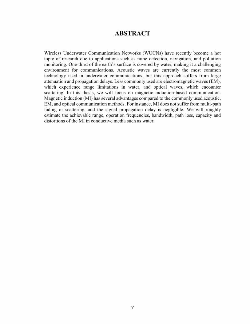
Wireless Underwater Communication Networks (WUCNs) have recently become a hot

topic of research due to applications such as mine detection, navigation, and pollution

monitoring. One-third of the earth’s surface is covered by water, making it a challenging

environment for communications. Acoustic waves are currently the most common

technology used in underwater communications, but this approach suffers from large

attenuation and propagation delays. Less commonly used are electromagnetic waves (EM),

which experience range limitations in water, and optical waves, which encounter

scattering. In this thesis, we will focus on magnetic induction-based communication.

Magnetic induction (MI) has several advantages compared to the commonly used acoustic,

EM, and optical communication methods. For instance, MI does not suffer from multi-path

fading or scattering, and the signal propagation delay is negligible. We will roughly

estimate the achievable range, operation frequencies, bandwidth, path loss, capacity and

distortions of the MI in conductive media such as water.

vi

LIST OF SYMBOLS USED

𝛿 Skin depth

휀 Electrical permittivity or dielectric constant

휀0 Electrical permittivity of free space ≈ 8.85 × 10−12 𝐹𝑚−1

휀𝑟 Relative permittivity

𝜆 Wavelength

𝜇 Magnetic permeability

𝜇0 Magnetic permeability of free space ≈ 4𝜋 × 10−7 𝐻𝑚−1

𝜇𝑟 Relative permeability

𝜌 Mass density

𝜎 Electrical conductivity

𝜙 Specific aperture (merit factor)

𝜔 Angular frequency, 𝜔 = 2𝜋𝑓

𝐵 Flux density

𝑐 Speed of light, ≈ 3 × 108 𝑚/𝑠

f Frequency

𝐹𝑎 Atmospheric noise temperature

𝐹𝑘 Atmospheric noise

𝐻 Magnetic field

𝑘 Boltzmann constant, ≈ 1.38 × 10−23𝐽𝑘−1

𝑘0 Wave number for free space

𝑚𝑑 Magnetic moment

vii

𝑁 Noise voltage or power

𝑆 Signal voltage or power

𝑇 Temperature [K]

𝑇𝑎 Atmospheric noise temperature

𝑍0 Wave impedance of free space, 𝑍0 = √𝜇0

0

viii

ACKNOWLEDGEMENTS

I would like to express my appreciation to my supervisor Schlegel who has

cheerfully answered my queries, provided me with materials, checked my

examples, assisted me in a myriad way with the writing and helpfully

commented on earlier drafts of this project. Also, I am very grateful to my

family and friends for their support throughout the production of this project.

CHAPTER1 INTRODUCTION

Traditional wireless networks that use EM suffer from high path loss, which limits their

communication range. To increase the EM range, a large antenna is used for low

frequencies, but this is unsuitable for small underwater vehicles. Optical waves experience

multiple scattering, limiting the application of optical signals to short-range distances.

Additionally, the transmission of optical signals requires a direct line of sight, which is

another challenge for mobile underwater vehicles and robots [10]. Radio waves suffer from

large attenuation and their range is limited to skin depth, which is associated with water

conductivity. Seawater has high conductivity, but the salinity and physical properties of

each type of seawater differ. Seawater measures around 4 S/m, whereas for pure water,

typical values range between 0.005 and 0.01 S/m [4].

Acoustic waves are widely used in underwater communication because they can travel long

distances. However, acoustic signals suffer from low bandwidth and data rates as well as

large propagation delays because the sound speed equals 1500 m/s [10]. Magnetic

induction (MI), however, is a promising solution for underwater short-range

communication.

MI technology has already proved to be a useful tool for underwater exploration. Due to

the high velocity of MI propagation, frequency offsets due to the Doppler effect are

negligible. Time-varying magnetic induction, generated by a primary coil or loop and

sensed by a secondary coil or loop, is the fundamental basis for magneto-inductive

communications. Transformers consisting of two coils positioned very close to each other

are the most common application of magnetic induction.

10

Ideally, total power is transferable from one coil to another. However, a regular magneto-

inductive communication system featuring a large distance between primary and secondary

coils rapidly experiences a power drop to a very small fraction. For this reason, coils are

usually asymmetric, meaning that the transmitter coils are large and heavy, whereas the

receiving coils are tiny and light [2]. A steering current drives the primary coil which

generates a reactive magnetic field and makes MI communication possible. By using such

a method, the energy stays local and is not transferrable at large distances that typical radio

waves can propagate. Thus, because the receiving signal strength will experience a rapid

decline over communication distance, it pushes MI communications out of the running as

an alternative to regular wireless communications.

MI communication has the potential to be used for underwater communications, as less

power loss occurs in comparison to electro-magnetic (EM) radio waves, which are rapidly

absorbed in water. From a theoretical communication perspective, MI channels do not

differ significantly from other electro-magnetic communication channels, and our

approach is generally standard in communication theory. However, there are some

differences between MI and RF communications, one of which is focusing on different

physical characteristics of the environment when developing practical channel models for

MI communications.

11

CHAPTER2 MI COMMUNICATION

MI communications use low-frequency modulation to enable reliable communication in

areas where traditional radio-frequency (RF) communications fails. These environments

include areas with a high concentration of conductive elements, through highly reflective

barriers such as the surface of water and communicating through the earth. So far, MI

communications has been limited to short ranges and low data rates but shows promise for

providing high-data throughput at short ranges. The communication scenario provides

unique opportunities and challenges. Additionally, given the nature of MI, it has not been

fully explored, which means that current systems operate far below capacity.

2.1 Related Work

Magnetic induction was first introduced as an underwater tool in [6], which featured a high-

speed link over a short range. In [8] and [1], underwater magneto-inductive networks were

analyzed using mutual coupling. Developing a model for magneto-inductive

communication was addressed in [7] by demonstrating the coupling between the coils in

the near field. In [3], a narrow bandwidth of a few KHz was reported because of the high

Q-factor (quality factor) of the magnetic coils. To expand the bandwidth [3], the front-end

resonant frequency was modulated in [14]. In [10], tuned resonant circuits (narrowband)

or unturned circuits (wideband) were applied to achieve high efficiency. Most of the

literature, such as [13], [9] and [12], demonstrates channel modeling from an end-to-end

perspective. So, for example, they focus not only the channel medium but also

12

on the characteristics of the transceiver and the coils. In this study, we focus on the channel

as a medium.

2.2 Background

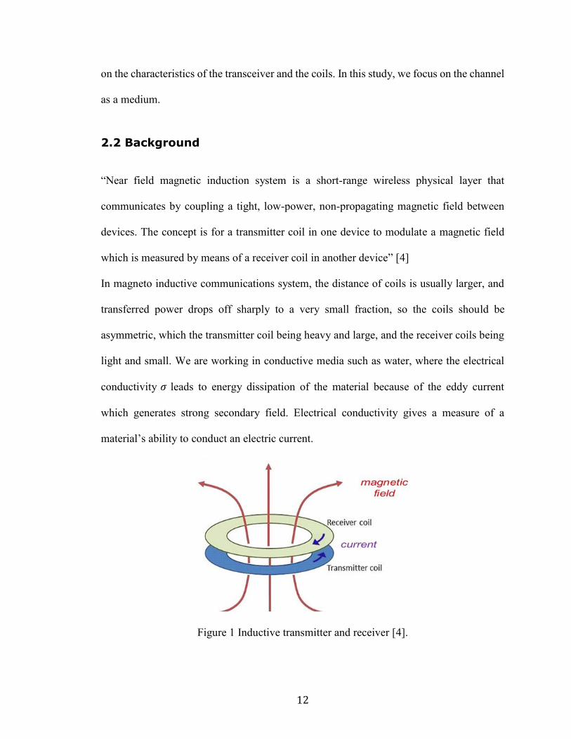
“Near field magnetic induction system is a short-range wireless physical layer that

communicates by coupling a tight, low-power, non-propagating magnetic field between

devices. The concept is for a transmitter coil in one device to modulate a magnetic field

which is measured by means of a receiver coil in another device” [4]

In magneto inductive communications system, the distance of coils is usually larger, and

transferred power drops off sharply to a very small fraction, so the coils should be

asymmetric, which the transmitter coil being heavy and large, and the receiver coils being

light and small. We are working in conductive media such as water, where the electrical

conductivity 𝜎 leads to energy dissipation of the material because of the eddy current

which generates strong secondary field. Electrical conductivity gives a measure of a

material’s ability to conduct an electric current.

Figure 1 Inductive transmitter and receiver [4].

13

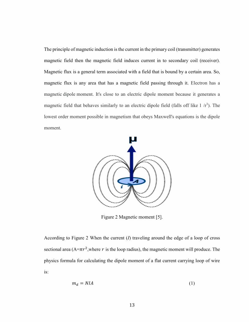
The principle of magnetic induction is the current in the primary coil (transmitter) generates

magnetic field then the magnetic field induces current in to secondary coil (receiver).

Magnetic flux is a general term associated with a field that is bound by a certain area. So,

magnetic flux is any area that has a magnetic field passing through it. Electron has a

magnetic dipole moment. It's close to an electric dipole moment because it generates a

magnetic field that behaves similarly to an electric dipole field (falls off like 1 /r3). The

lowest order moment possible in magnetism that obeys Maxwell's equations is the dipole

moment.

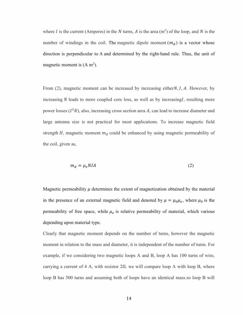
Figure 2 Magnetic moment [5].

According to Figure 2 When the current (I) traveling around the edge of a loop of cross

sectional area (A=𝜋𝑟2,where 𝑟 is the loop radius), the magnetic moment will produce. The

physics formula for calculating the dipole moment of a flat current carrying loop of wire

is:

𝑚𝑑 = 𝑁𝐼𝐴 (1)

14

where 𝐼 is the current (Amperes) in the 𝑁 turns, 𝐴 is the area (m2) of the loop, and 𝑁 is the

number of windings in the coil. The magnetic dipole moment (𝑚𝑑 ) is a vector whose

direction is perpendicular to A and determined by the right-hand rule. Thus, the unit of

magnetic moment is (A m2).

From (2), magnetic moment can be increased by increasing either𝑁, 𝐼, 𝐴. However, by

increasing 𝑁 leads to more coupled core loss, as well as by increasing𝐼, resulting more

power losses (𝐼2𝑅), also, increasing cross section area 𝐴, can lead to increase diameter and

large antenna size is not practical for most applications. To increase magnetic field

strength 𝐻, magnetic moment 𝑚𝑑 could be enhanced by using magnetic permeability of

the coil, given as,

𝑚𝑑 = 𝜇𝑒𝑁𝐼𝐴 (2)

Magnetic permeability 𝜇 determines the extent of magnetization obtained by the material

in the presence of an external magnetic field and denoted by 𝜇 = 𝜇0𝜇𝑒, where 𝜇0 is the

permeability of free space, while 𝜇𝑒 is relative permeability of material, which various

depending upon material type.

Clearly that magnetic moment depends on the number of turns, however the magnetic

moment in relation to the mass and diameter, it is independent of the number of turns. For

example, if we considering two magnetic loops A and B, loop A has 100 turns of wire,

carrying a current of 4 A, with resistor 2Ω. we will compare loop A with loop B, where

loop B has 500 turns and assuming both of loops have an identical mass.so loop B will

15

have five times the length of wire and resistance will be 25 times greater that is because

five times greater due to length and another five times greater due to small cross section

area. So, to get the same magnetic moment as loop A, it needs only 1/5 of the current (i.e.

0.8 A). Resulting in power dissipation 𝐼2𝑅 for loop A is 32w as well as for loop B is 32w.

The magnetic field strength =𝑚𝑑

4𝜋𝑟3 , at a coaxial point at distance 𝑟 from the loop antenna

is proportional to the magnetic moment and decreases with the third power of 𝑟. Magnetic

field strength can be increased by increasing magnetic moment.

16

CHAPTER3 METHODOLOGIES

The methodologies we are adapting here quite standard in the field of communication

theory.

3.1 The Magneto Inductive Channel

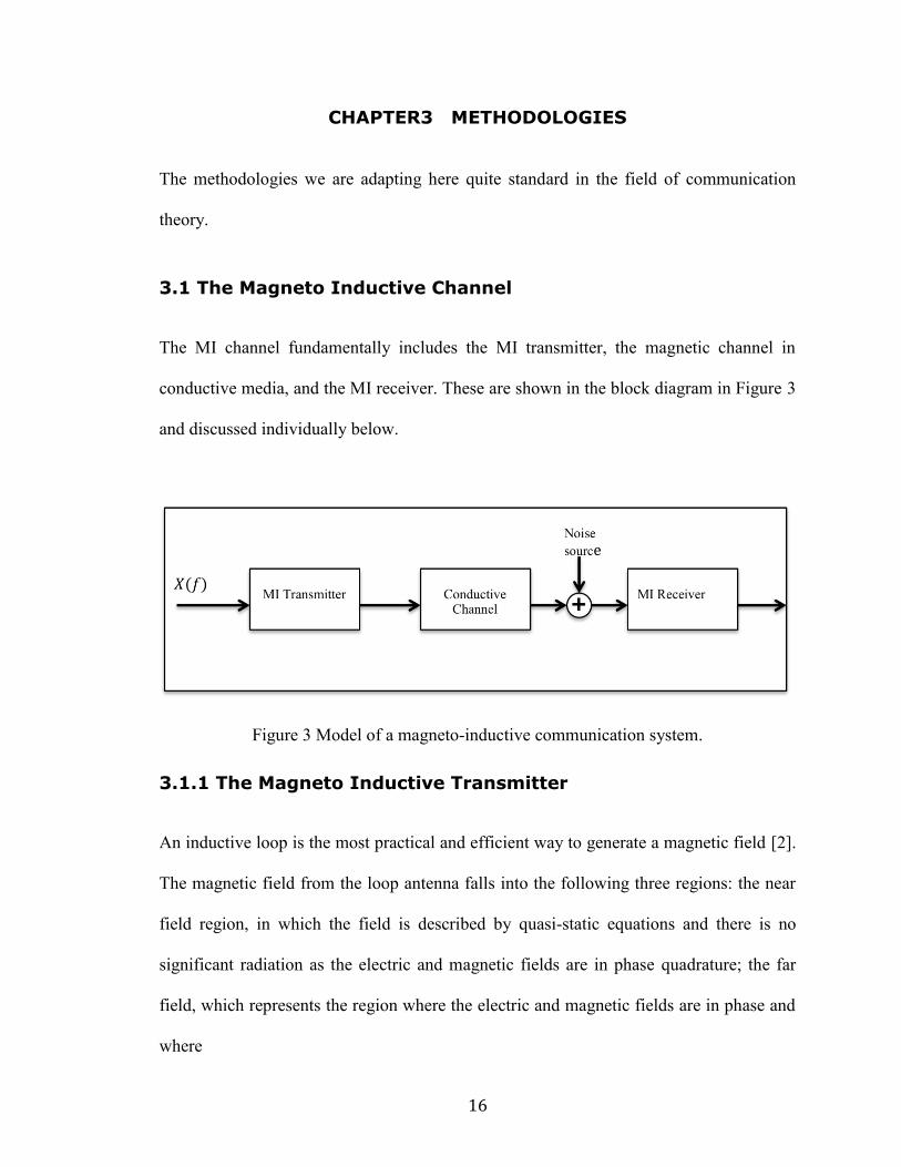
The MI channel fundamentally includes the MI transmitter, the magnetic channel in

conductive media, and the MI receiver. These are shown in the block diagram in Figure 3

and discussed individually below.

Figure 3 Model of a magneto-inductive communication system.

3.1.1 The Magneto Inductive Transmitter

An inductive loop is the most practical and efficient way to generate a magnetic field [2].

The magnetic field from the loop antenna falls into the following three regions: the near

field region, in which the field is described by quasi-static equations and there is no

significant radiation as the electric and magnetic fields are in phase quadrature; the far

field, which represents the region where the electric and magnetic fields are in phase and

where

17

the magnetic field peels off as a propagating electro-magnetic wave; and the transition

region, which is located between the near and far field regions [2].

Table 1 Showing the boundary conditions of the near field, transition zone, and far-

field.

As we can see from Table 1 boundary conditions of the three regions using two common

measures (wavenumber |𝒌𝟎|and skin depth 𝜹), where is the 𝑻 the ratio of distance to skin

depth, given as 𝑻 =𝐫

𝛅 and 𝒌𝟎 =

𝟐𝛑𝐟

𝐜. We are primarily interested in the near field, for which

𝐫 < 𝛅 and

T =r

δ< 1 (3.1)

where r is the operating distance and T is skin depth numbers.

The magnetic near-field decays with the inverse cube of the distance. According to the Biot

– Savart Law, the magnetic field from a small element is proportional to (1

𝑟3).

𝑩 =𝝁𝟎

𝟒𝝅∫ 𝑰

𝒅𝑰×𝒓

𝒓𝟑 (3.2)

where 𝐵 is the flux density and 𝐼 is the current (see Figure 4).

Properties

Near–field

approximation

Transition region

approximation

Far-field

approximation

Skin depth 𝑇 ≪ 1 𝑇2 ≪ 1 𝑇 ≫ 1

Wave number 𝑘0𝑟 ≪ 1 (𝑘0𝑟)2 ≪ 1 𝑘0𝑟 ≫ 1

18

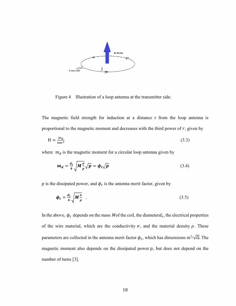
Figure 4 Illustration of a loop antenna at the transmitter side.

The magnetic field strength for induction at a distance r from the loop antenna is

proportional to the magnetic moment and decreases with the third power of 𝑟, given by

H =md

4πr3 (3.3)

where 𝑚𝑑 is the magnetic moment for a circular loop antenna given by

𝒎𝒅 =𝒅𝒕

𝟒√𝑴

𝝈

𝝆√𝒑 = 𝝓𝒕√𝒑 (3.4)

𝑝 is the dissipated power, and 𝜙𝑡 is the antenna merit factor, given by

𝝓𝒕 =𝒅𝒕

𝟒√𝑴

𝝈

𝝆 . (3.5)

In the above, 𝜙𝑡 depends on the mass 𝑀of the coil, the diameter𝑑𝑡, the electrical properties

of the wire material, which are the conductivity 𝜎 , and the material density 𝜌 . These

parameters are collected in the antenna merit factor 𝜙𝑡, which has dimensions m2/√Ω. The

magnetic moment also depends on the dissipated power 𝑝, but does not depend on the

number of turns [3].

19

For example, consider a portable induction loop antenna, where the diameter is 1m and

mass is 0.6 Kg. If we take into account that the loop is made from copper √𝜎

𝜌 =8m/Kg√Ω,

the magnetic moment is 50 Am2 with a power dissipation of 10 w.

The 𝐻-field is directly proportional to the loop current. Hence, since the power loss in the

antenna (which is due to ohmic resistance) is also directly proportional to the loop current,

there is no fundamental preference of frequency [2].

3.1.2 The Communications Channel

Communication through conductive media such as seawater is possible only over distances

of a few skin depths. The skin depth gives a measure of the penetration of magnetic field

into a given medium. The magnetic field decays with distance into the medium, and this

decay of the field is expressed by the skin depth, given by [3]

𝜹 = √𝟐

𝝎𝝁𝝈 (3.6)

where:

𝜇 = 4𝜋 × 10−7 𝑁 𝐴−2⁄ (Magnetic permeability in vacuum)

𝜔 = 2𝜋𝑓 (Angular frequency)

𝜎 : Electrical conductivity in siemens/meter

The penetration of the magnetic field into the conductive medium obeys Maxwell’s

equations:

△× 𝑯 = (𝒋𝝎𝜺 + 𝝈). (Ampere’s law) (3.7)

20

Electromagnetic waves in a vacuum obey a standard type of partial differential equation

(PDE) called the "wave equation". However, in a conductive medium, where the angular

frequency is much less than sigma/epsilon, they obey a different type of partial

differential equation, known as the "diffusion equation".

If ω ≪ σ ϵ,⁄ the propagation equation of the magnetic field turns into the diffusion

equation, which means diffusion properties of electromagnetic waves are mainly

dependent on the conductivity and propagation behavior of the wave is an important aspect

of time.

△𝟐 𝑯 = 𝒋𝝎𝝁𝝈𝑯. (3.8)

The magnetic field is attenuated according to the skin depth. In a good conductor with

(𝜎

𝜔≫ 1) , such as seawater, a large skin depth attenuation is experienced. If we assume

an operating frequency of 1 MHz, the skin depth for seawater is 0.25m with a wavelength

of 1.6m. This means the frequency within the LF (30-300 kHz) or the VLF (3-30 kHz)

bands would be the most optimal, as skin depth is inversely proportional to the square root

of the frequency used.

A basic model for the magnetic field penetration consists of a cubic distance attenuation

combined with an exponential absorption loss given by [2]

|𝑨(𝝎, 𝒓)| =𝐐(𝐓)

𝟒𝛑𝐫𝟑 . (3.9)

The attenuation Q(T) represents the exponential medium losses at a rate of 8.7 dB per skin

depth. It is frequency-dependent, since δ is frequency-dependent and has general low-pass

characteristics. It is given by

𝑄(𝑇) = 2𝑒−𝑇√𝑇2 + (1 + 𝑇)2. (3.10)

21

The total absorption is the combination the cubic distance attenuation of (3.9) and the

exponential absorption loss in (3.10).

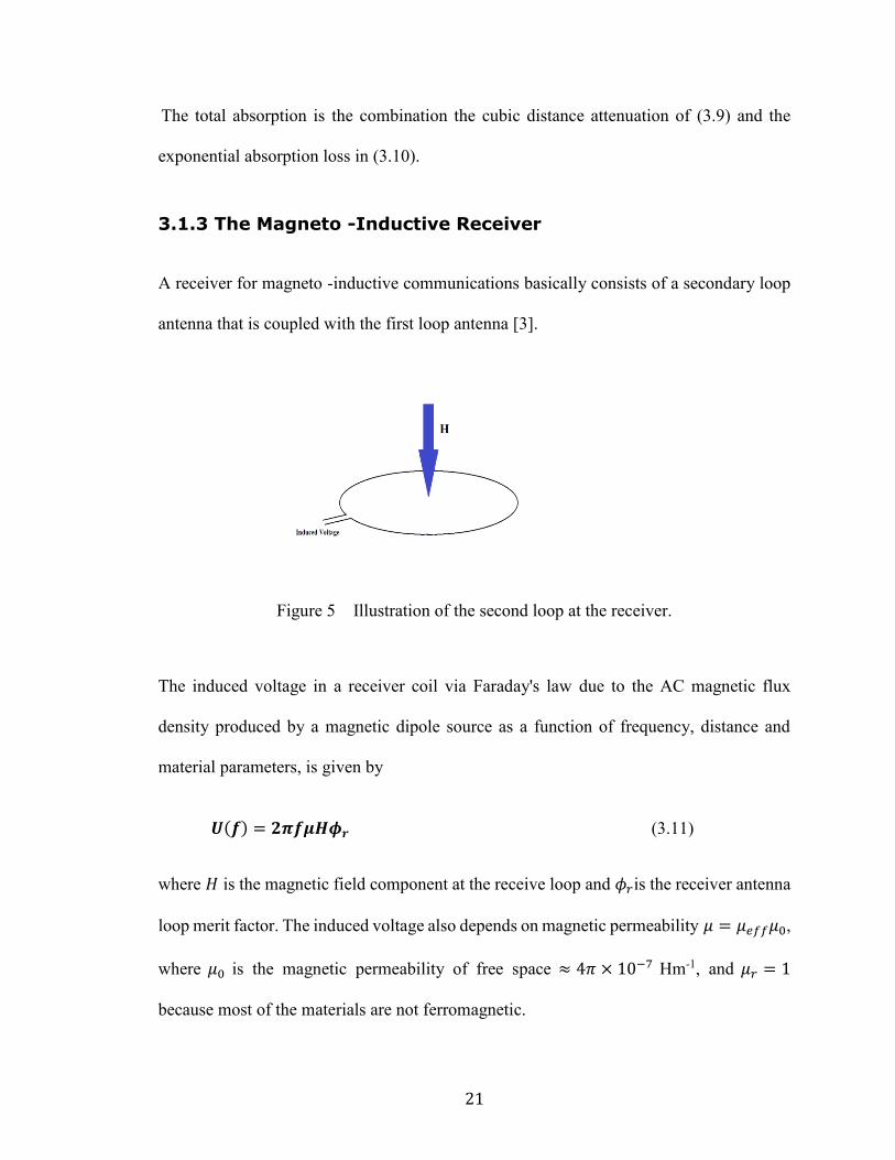
3.1.3 The Magneto -Inductive Receiver

A receiver for magneto -inductive communications basically consists of a secondary loop

antenna that is coupled with the first loop antenna [3].

Figure 5 Illustration of the second loop at the receiver.

The induced voltage in a receiver coil via Faraday's law due to the AC magnetic flux

density produced by a magnetic dipole source as a function of frequency, distance and

material parameters, is given by

𝑼(𝒇) = 𝟐𝝅𝒇𝝁𝑯𝝓𝒓 (3.11)

where 𝐻 is the magnetic field component at the receive loop and 𝜙𝑟is the receiver antenna

loop merit factor. The induced voltage also depends on magnetic permeability 𝜇 = 𝜇𝑒𝑓𝑓𝜇0,

where 𝜇0 is the magnetic permeability of free space ≈ 4𝜋 × 10−7 Hm-1, and 𝜇𝑟 = 1

because most of the materials are not ferromagnetic.

22

In a good conductor with (𝜎

𝜔≫ 1), and if the communication range is within the near field,

(𝑇 ≪ 1), the optimal frequency for a given distance r is given by

𝑓 =𝑇2

𝜋𝑟2𝜇𝜎 . (3.10)

by substituting (3.12) in (3.11) to derive the induced voltage in a coaxial receiver loop as

Uinduced ≈ ϕ√Rmd

2πσ .

1

r5 T2 Q(T) . (3.11)

As the frequency goes to zero, the skin depth 𝛿 becomes large and T→ 0 so the induced

voltage tends to zero. This is due to the lack of magnetic induction at frequency 0.

Likewise, at a high frequency, 𝛿 becomes small and T → ∞ so e−T → 0. As a result, there

is no signal because of the greater degree in skin depth attenuation [3].

3.2 Channel with Noise

The term ‘noise’ refers to unwanted electrical signals that are always present in electrical

systems. Signal transmission through any channel suffers from additive noise, which can

be generated internally by the components such as resistors and solid-state devices used to

implement the communication system. This is called thermal noise. Such noise can also be

generated externally as a result of interference from other channel users. Noise is one of

the limiting factors in a communication system because when noise is added to the signal,

it is impossible to transmit a near infinite amount of information over a finite bandwidth

communication system.

23

3.2.1 Thermal Noise

Thermal noise is generated due to the random movement of electrons inside the volume of

conductors or resistors even in the absence of electric field. If the noise at the receiver is

purely thermal, its normalized noise power spectral density is given by:

𝑁(𝑓) = 4𝑘𝑇 (3.14)

where k = 1.38 × 10−23 J/K is Boltzmann’s constant, and T is the receiver temperature in

Kelvin [2].

3.2.2 Atmospheric Noise

Atmospheric noise is a collective term of all noise sources that are not local thermal. A

typical example of atmospheric noise is receiver noise. It may be caused by the electrical

activity in the atmosphere as well as by man-made electrical disturbances. In lower

frequency ranges, ambient noise is picked up by the antenna, especially if the antenna is at

the surface and dominates over thermal noise. Therefore, it is preferable to use a noise

model that is analogous to the thermal noise. In the following, we define the atmospheric

noise power density as

𝑁(𝑓) = 4𝑘𝑇𝐹𝑎(𝑓) 𝑅𝑟 𝑅 ⁄ (3.15)

where Rr is the radiation resistance of the antenna, R is the ohmic resistance of the receiver

coil, and 𝐹a is the atmospheric noise temperature given by

24

𝐹𝑎(𝑓) =6𝜋

𝑘02

𝑍0𝐻2

4𝑘𝑇 (3.16)

where k0 is the wave number and is equal to k0 =2πf

c (where 𝑐 is the speed of light) and

Z0 is the impedance of free space. Z0 also equals the ratio of the electric field component

to the magnetic field component Z0 =|E|

|H| and is approximately 377 Ohm.

We can use (3.16) to deliver the atmospheric noise as a function of frequency and

atmospheric noise temperature in the following

𝐹𝑘 = √𝐹𝑎𝑍0𝑘0

4

6𝜋 (3.17)

20𝑙𝑜𝑔𝐹𝑘 = 10𝑙𝑜𝑔𝐹𝑎 + 40𝑙𝑜𝑔𝑓 − 294.147 (3.18)

3.3 Channel Capacity

Long before wireless communication dominated our daily lives, research had established

fundamental limits on the rate at which we could communicate over wireless channels. One

of the most important theorems is the Shannon capacity theorem, which sets an upper

bound on how fast we can transmit information over a particular wireless link. There is no

way to exceed this theoretical upper bound, but we can get close to it.

The Shannon capacity formula for a flat channel with white Gaussian noise is given by

𝒄 = 𝒘𝒍𝒐𝒈𝟐(𝟏 +𝒔

𝑵) (3.19)

where w is Bandwidth in (Hz) , and 𝑆

𝑁 is the signal –to- noise ratio.

25

The capacity is directly proportional to the bandwidth. If we have a wider bandwidth to

communicate, we can send more data. This is important because we will look at how

bandwidth is allocated in terms of different frequency bands.

We can generalize instances of frequency-dependent signals and noise spectral powers

𝑆(𝑓) and 𝑁(𝑓) in the following way:

𝑐 = ∑ △ 𝑓 log (1 +𝑆(𝑓1+𝑖△𝑓)△𝑓

𝑁(𝑓1+𝑖△𝑓)△𝑓)𝑁

𝑖=0 → ∫ log (1 +𝑆(𝑓)

𝑁(𝑓))

𝑓2

𝑓1𝑑𝑓 (3.20)

where f1 is the lower band edge, f2=f1+𝑁𝛿f is the upper band edge, and f2-f1=w is the

channel bandwidth.

26

CHAPTER4 RESULTS AND DISCUSSION

In this study, all the graphs are done by using Matlab software and some of our results are

summarized into tables.

4.1 MI Channel

Frequency should be as low as possible to avoid eddy current which produce strong

secondary field. skin depth is frequency dependent (3.6), so in Figure 6 will show the

skin depth as a function of frequency for seawater (𝜎 = 4𝑆/𝑚) and fresh water (𝜎 =

0.01𝑆/𝑚).

Figure 6 Skin depths as a function of frequency and conductivity for both seawater and

fresh water.

Frequency (Hz)10

110

210

310

410

5

skin

de

pth

(m

)

10-1

100

101

102

103

104

skin depth vs. Frequency - for different conductivity

conductivity=4S/mfresh waterconductivity=0.01S/m

27

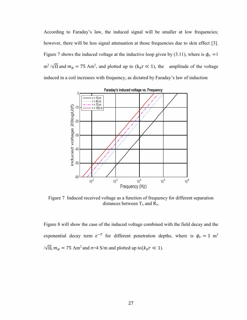
According to Faraday’s law, the induced signal will be smaller at low frequencies;

however, there will be less signal attenuation at those frequencies due to skin effect [3].

Figure 7 shows the induced voltage at the inductive loop given by (3.11), where is 𝜙𝑟 =1

m2 /√Ω and 𝑚𝑑 = 75 Am2, and plotted up to (k0r ≪ 1), the amplitude of the voltage

induced in a coil increases with frequency, as dictated by Faraday’s law of induction

Figure 7 Induced received voltage as a function of frequency for different separation

distances between Tx and Rx.

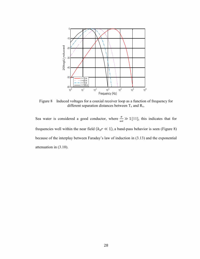
Figure 8 will show the case of the induced voltage combined with the field decay and the

exponential decay term 𝑒−𝑇 for different penetration depths, where is 𝜙𝑟 = 1 m2

/√Ω, 𝑚𝑑 = 75 Am2 and σ=4 S/m and plotted up to(𝑘0𝑟 ≪ 1).

Frequency (Hz)10

210

310

410

510

6

ind

uce

d v

olta

ge

20

log

U(f)

-60

-50

-40

-30

-20

-10

0Faraday's induced voltage vs. Frequency

r = 10 mr = 40 mr = 70 mr = 100 m

28

Figure 8 Induced voltages for a coaxial receiver loop as a function of frequency for

different separation distances between Tx and Rx.

Sea water is considered a good conductor, where 𝜎

𝜔≫ 1 [11], this indicates that for

frequencies well within the near field (𝑘0𝑟 ≪ 1), a band-pass behavior is seen (Figure 8)

because of the interplay between Faraday’s law of induction in (3.13) and the exponential

attenuation in (3.10).

Frequency (Hz)10

010

110

210

310

410

510

6

20

log

Uin

duced

-60

-50

-40

-30

-20

-10

0

r = 10 mr = 40 mr = 70 mr = 100 m

29

4.2 Channel Attenuation

In MI, the channel attenuation is calculated by combining the cubic distance and the

exponential absorption, given in (3.9).

Figure 9 shows the attenuation |A (ω, r)| of an MI channel as a function of distance and

frequency for seawater with a typical value of σ = 4S/m.

Figure 9 Distance and frequency dependent attenuation of the magneto-inductive signal

for a typical value of σ=4S/m for seawater.

We modified the previous simulation (which is not valid for making the decision) from 3-

dimensional to 2-dimensional (see Figure 10). Our reason for doing this is that the skin

depth depends on the frequency while the T ratio depends on distance and skin depth, and

different frequencies can cover different distances. Furthermore, when we plot all

frequencies together, higher frequencies need a lower skin depth and a lower distance,

whereas lower frequencies need higher skin depth and longer distance. Therefore,

30

integrating both high and low frequencies in the same plot and ensuring that all are “near-

field” regions means that we should stick to the simulation of the lowest distance, which

can be accessed by the highest frequencies. Thus, we changed the code and performed the

simulation for different frequencies over a distance that can meet near-field criteria.

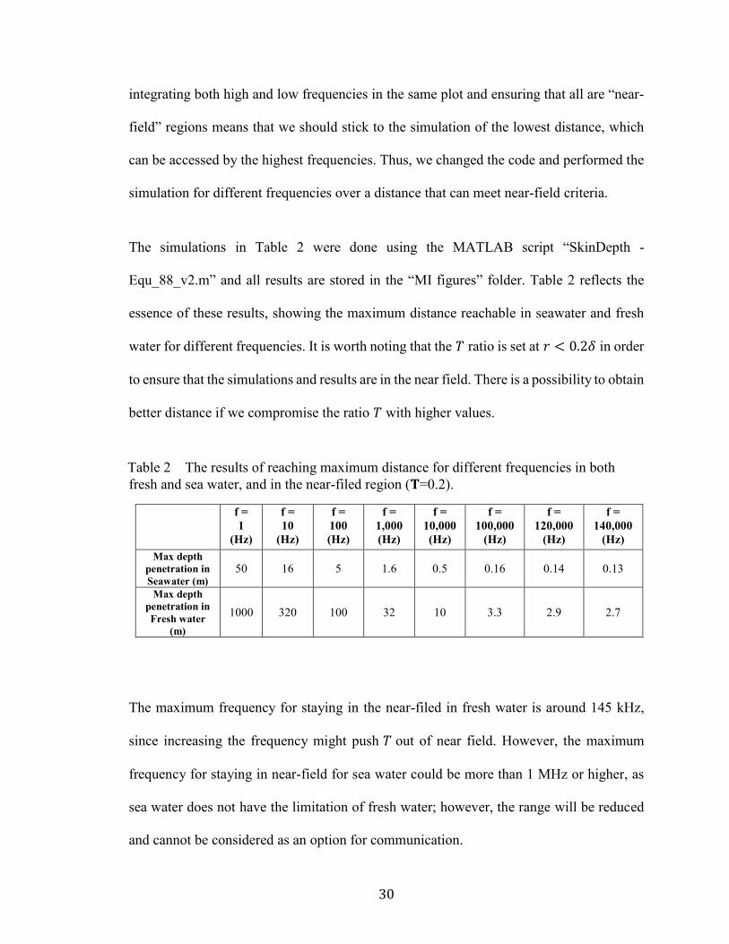
The simulations in Table 2 were done using the MATLAB script “SkinDepth -

Equ_88_v2.m” and all results are stored in the “MI figures” folder. Table 2 reflects the

essence of these results, showing the maximum distance reachable in seawater and fresh

water for different frequencies. It is worth noting that the 𝑇 ratio is set at 𝑟 < 0.2𝛿 in order

to ensure that the simulations and results are in the near field. There is a possibility to obtain

better distance if we compromise the ratio 𝑇 with higher values.

Table 2 The results of reaching maximum distance for different frequencies in both

fresh and sea water, and in the near-filed region (𝐓=0.2).

f =

1

(Hz)

f =

10

(Hz)

f =

100

(Hz)

f =

1,000

(Hz)

f =

10,000

(Hz)

f =

100,000

(Hz)

f =

120,000

(Hz)

f =

140,000

(Hz)

Max depth

penetration in

Seawater (m)

50 16 5 1.6 0.5 0.16 0.14 0.13

Max depth

penetration in

Fresh water

(m)

1000 320 100 32 10 3.3 2.9 2.7

The maximum frequency for staying in the near-filed in fresh water is around 145 kHz,

since increasing the frequency might push 𝑇 out of near field. However, the maximum

frequency for staying in near-field for sea water could be more than 1 MHz or higher, as

sea water does not have the limitation of fresh water; however, the range will be reduced

and cannot be considered as an option for communication.

31

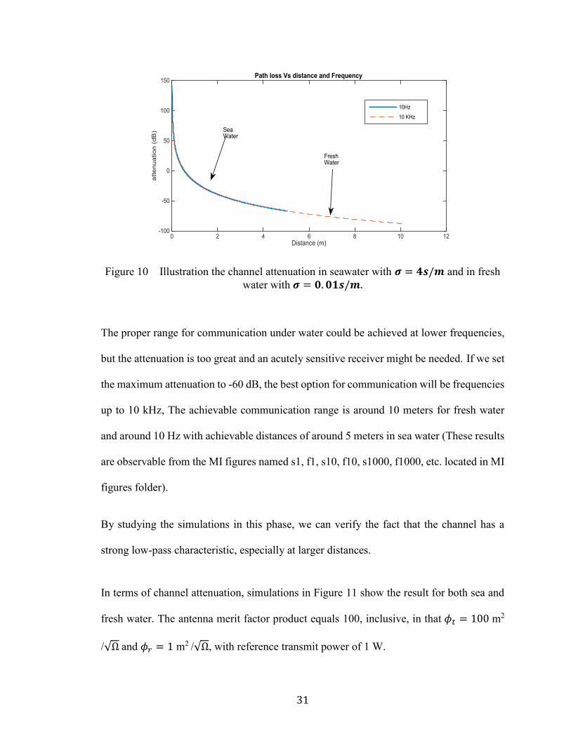
Figure 10 Illustration the channel attenuation in seawater with 𝝈 = 𝟒𝒔/𝒎 and in fresh

water with 𝝈 = 𝟎. 𝟎𝟏𝒔/𝒎.

The proper range for communication under water could be achieved at lower frequencies,

but the attenuation is too great and an acutely sensitive receiver might be needed. If we set

the maximum attenuation to -60 dB, the best option for communication will be frequencies

up to 10 kHz, The achievable communication range is around 10 meters for fresh water

and around 10 Hz with achievable distances of around 5 meters in sea water (These results

are observable from the MI figures named s1, f1, s10, f10, s1000, f1000, etc. located in MI

figures folder).

By studying the simulations in this phase, we can verify the fact that the channel has a

strong low-pass characteristic, especially at larger distances.

In terms of channel attenuation, simulations in Figure 11 show the result for both sea and

fresh water. The antenna merit factor product equals 100, inclusive, in that 𝜙𝑡 = 100 m2

/√Ω and 𝜙𝑟 = 1 m2 /√Ω, with reference transmit power of 1 W.

Distance (m)0 2 4 6 8 10 12

att

enu

atio

n (

dB

)

-100

-50

0

50

100

150Path loss Vs distance and Frequency

10Hz

10 KHz

SeaWater

FreshWater

32

Figure 11 System transfer function 𝑯(𝒇) with different penetration depths for both

seawater and fresh water.

In Figure 11, for both seawater and fresh water, atmospheric noise refers to atmospheric

noise temperature. The reference power is also 1 w (0 dBW). It should be noted that the

optimal transmission range depends on the received SNR, which itself depends on the

transfer function as a distance dependent factor (more distance, more attenuation) and the

transmitter power. We can see this by looking at Figure 11 and setting the first necessity

as a channel with a flat bandwidth. Tables 4 and 5 reflect the details of the channel

bandwidth over different ranges of communications for sea and fresh water, respectively.

The bandwidth has been calculated using Figure 11. The -3dB bandwidth occurs when the

channel attenuation drops for 3dB from its value at f=1KHz. So, for example, for seawater

with a communication range of 100m, the attenuation at f=1Hz is -101.5 dB. Thus, the -

3dB bandwidth occurs when the attenuation drops an extra 3dB(-101.5 –3 = -104.5 dB).

The point (around 10 Hz) can be found in Figure 10. By performing the same calculations

for all frequencies in both seawater and fresh water, the results would be as shown in Tables

Frequency (Hz)10

010

110

210

310

410

510

6

H(d

B)

-300

-250

-200

-150

-100

-50

0Transfer Function (Channel)-Sea Water and Fresh Water

100m200m300m400m500mAtmospheric Noise

SeaWater

FreshWater

33

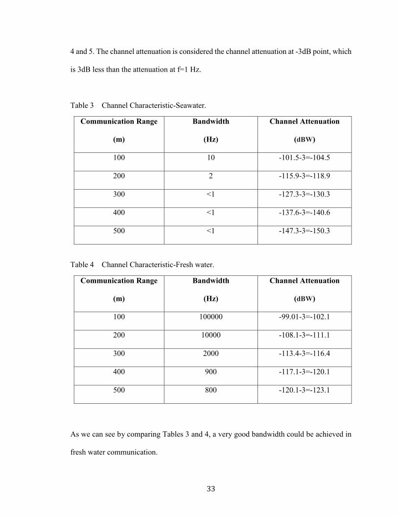
4 and 5. The channel attenuation is considered the channel attenuation at -3dB point, which

is 3dB less than the attenuation at f=1 Hz.

Table 3 Channel Characteristic-Seawater.

Communication Range

(m)

Bandwidth

(Hz)

Channel Attenuation

(dBW)

100 10 -101.5-3=-104.5

200 2 -115.9-3=-118.9

300 <1 -127.3-3=-130.3

400 <1 -137.6-3=-140.6

500 <1 -147.3-3=-150.3

Table 4 Channel Characteristic-Fresh water.

Communication Range

(m)

Bandwidth

(Hz)

Channel Attenuation

(dBW)

100 100000 -99.01-3=-102.1

200 10000 -108.1-3=-111.1

300 2000 -113.4-3=-116.4

400 900 -117.1-3=-120.1

500 800 -120.1-3=-123.1

As we can see by comparing Tables 3 and 4, a very good bandwidth could be achieved in

fresh water communication.

34

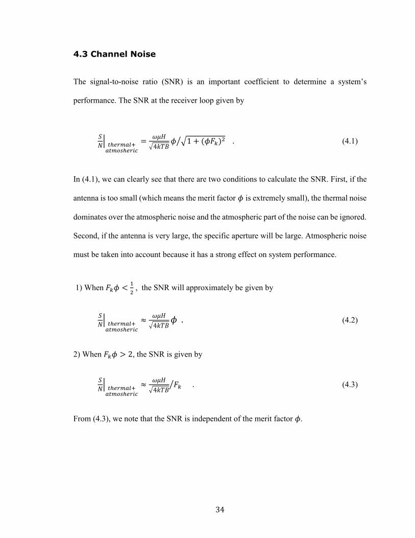
4.3 Channel Noise

The signal-to-noise ratio (SNR) is an important coefficient to determine a system’s

performance. The SNR at the receiver loop given by

𝑆

𝑁|

𝑡ℎ𝑒𝑟𝑚𝑎𝑙+𝑎𝑡𝑚𝑜𝑠ℎ𝑒𝑟𝑖𝑐

=𝜔𝜇𝐻

√4𝑘𝑇𝐵𝜙 √1 + (𝜙𝐹𝑘)2⁄ . (4.1)

In (4.1), we can clearly see that there are two conditions to calculate the SNR. First, if the

antenna is too small (which means the merit factor 𝜙 is extremely small), the thermal noise

dominates over the atmospheric noise and the atmospheric part of the noise can be ignored.

Second, if the antenna is very large, the specific aperture will be large. Atmospheric noise

must be taken into account because it has a strong effect on system performance.

1) When 𝐹𝑘𝜙 <1

2 , the SNR will approximately be given by

𝑆

𝑁|

𝑡ℎ𝑒𝑟𝑚𝑎𝑙+𝑎𝑡𝑚𝑜𝑠ℎ𝑒𝑟𝑖𝑐

≈𝜔𝜇𝐻

√4𝑘𝑇𝐵𝜙 . (4.2)

2) When 𝐹𝑘𝜙 > 2, the SNR is given by

𝑆

𝑁|

𝑡ℎ𝑒𝑟𝑚𝑎𝑙+𝑎𝑡𝑚𝑜𝑠ℎ𝑒𝑟𝑖𝑐

≈𝜔𝜇𝐻

√4𝑘𝑇𝐵𝐹𝑘⁄ . (4.3)

From (4.3), we note that the SNR is independent of the merit factor 𝜙.

35

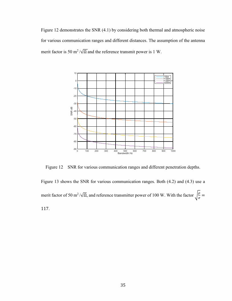
Figure 12 demonstrates the SNR (4.1) by considering both thermal and atmospheric noise

for various communication ranges and different distances. The assumption of the antenna

merit factor is 50 m2 /√Ω and the reference transmit power is 1 W.

Figure 12 SNR for various communication ranges and different penetration depths.

Figure 13 shows the SNR for various communication ranges. Both (4.2) and (4.3) use a

merit factor of 50 m2 /√Ω, and reference transmitter power of 100 W. With the factor √𝜌

𝜎=

117.

Bandwidth Hz0 100 200 300 400 500 600 700 800 900 1000

SN

R d

B

-90

-80

-70

-60

-50

-40

-30

-20

-10

0

10

r=50mr=100mr=150mr=200m

36

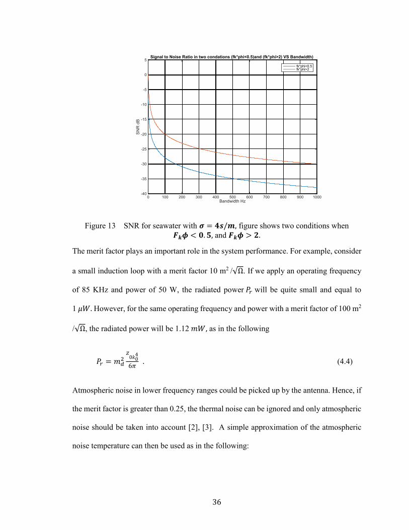
Figure 13 SNR for seawater with 𝝈 = 𝟒𝒔/𝒎, figure shows two conditions when

𝑭𝒌𝝓 < 𝟎. 𝟓, and 𝑭𝒌𝝓 > 𝟐.

The merit factor plays an important role in the system performance. For example, consider

a small induction loop with a merit factor 10 m2 /√Ω. If we apply an operating frequency

of 85 KHz and power of 50 W, the radiated power 𝑃𝑟 will be quite small and equal to

1 𝜇𝑊. However, for the same operating frequency and power with a merit factor of 100 m2

/√Ω, the radiated power will be 1.12 𝑚𝑊, as in the following

𝑃𝑟 = 𝑚𝑑2

𝑧0𝑘0

4

6𝜋 . (4.4)

Atmospheric noise in lower frequency ranges could be picked up by the antenna. Hence, if

the merit factor is greater than 0.25, the thermal noise can be ignored and only atmospheric

noise should be taken into account [2], [3]. A simple approximation of the atmospheric

noise temperature can then be used as in the following:

Bandwidth Hz0 100 200 300 400 500 600 700 800 900 1000

SN

R d

B

-40

-35

-30

-25

-20

-15

-10

-5

0

5Signal to Noise Ratio in two condations (fk*phi<0.5)and (fk*phi>2) VS Bandwidth)

fk*phi<0.5fk*phi>2

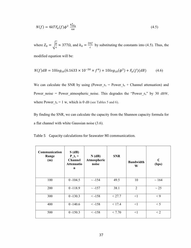
37

𝑁(𝑓) = 4𝑘𝑇𝐹𝑎(𝑓)𝜙2 𝑘0𝑍0

4

6𝜋 (4.5)

where 𝑍0 = √𝜇

𝜖≈ 377Ω, and 𝑘0 =

2𝜋𝑓

𝑐 by substituting the constants into (4.5). Thus, the

modified equation will be:

𝑁(𝑓)𝑑𝐵 = 10𝑙𝑜𝑔10(6.1633 × 10−50 × 𝑓4) + 10𝑙𝑜𝑔10(𝜙2) + 𝐹𝑎(𝑓)(𝑑𝐵) (4.6)

We can calculate the SNR by using (Power_rx = Power_tx + Channel attenuation) and

Power_noise = Power_atmospheric_noise. This degrades the “Power_rx” by 30 dBW,

where Power_tx = 1 w, which is 0 dB (see Tables 5 and 6).

By finding the SNR, we can calculate the capacity from the Shannon capacity formula for

a flat channel with white Gaussian noise (3.6).

Table 5 Capacity calculations for Seawater MI communication.

Communication

Range

(m)

S (dB)

P_tx +

Channel

Attenuatio

n

N (dB)

Atmospheric

noise

SNR

Bandwidth

W

𝐂

(bps)

100 0 -104.5 ~ -154 49.5 10 ~ 164

200 0 -118.9 ~ -157 38.1 2 ~ 25

300 0 -130.3 < -158 < 27.7 <1 < 9

400 0 -140.6 < -158 < 17.4 <1 < 5

500 0 -150.3 < -158 < 7.70 <1 < 2

38

Table 6 Capacity calculation for Fresh water MI communication.

Communication

Range

(m)

S (dB)

P_tx +

Channel

Attenuation

N (dB)

Atmospheric

noise

SNR

Bandwidth

W

𝑪

(bps)

100 0-102.1 ~ -140 37.99 100000 315,510

200 0-111.1 ~ - 143 31.90 10000 48,326

300 0-116.4 ~ -145 28.6 2000 15,946

400 0-120.1 ~ -146 25.9 900 6938

500 0-123.1 ~ -147 23.9 800 3639

Note that the Capacity and communication range are significantly better for fresh water

communication.

4.4 Up-link and Downlink Operation

The main impact of atmospheric noise is on uplink and downlink operations, with the effect

being different for the uplink compared to the downlink. Specifically, in the uplink, the full

value of atmospheric noise will be present, while in the downlink, atmospheric noise will

attenuate as 8.7 per skin depth.

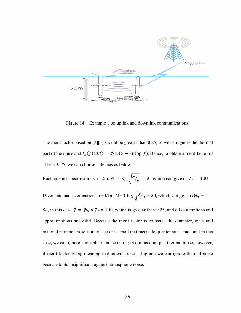
In this example (Figure 14), we will consider communication between a boat located on

the surface and diver carrying the other coil. The maximum depth for divers to

communication will be 50m.

39

Figure 14 Example 1 on uplink and downlink communications.

The merit factor based on [2][3] should be greater than 0.25, so we can ignore the thermal

part of the noise and 𝐹𝑎(𝑓)(𝑑𝐵) = 294.15 − 36 log(𝑓). Hence, to obtain a merit factor of

at least 0.25, we can choose antennas as below

Boat antenna specifications: r=2m, M= 4 Kg, √𝜎𝜌⁄ = 50, which can give us ∅𝑏 = 100

Diver antenna specifications: r=0.1m, M= 1 Kg, √𝜎𝜌⁄ = 20, which can give us ∅𝑑 = 1

So, in this case, ∅ = ∅𝑏 × ∅𝑑 = 100, which is greater than 0.25, and all assumptions and

approximations are valid. Because the merit factor is collected the diameter, mass and

material parameters so if merit factor is small that means loop antenna is small and in this

case, we can ignore atmospheric noise taking in our account just thermal noise, however,

if merit factor is big meaning that antenna size is big and we can ignore thermal noise

because to its insignificant against atmospheric noise.

40

The communication range is maximum 50m, and since we are working in near-field and

T<<1 (T=0.2 in our MATLAB code), T =r

δ<< 1, as we assumed 0.2 during our previous

simulations.

Next, in finding 𝛿 =50

0.2= 250 m, we need to find the maximum working frequency 𝛿 =

√2

𝜔𝜇𝜎. By making frequency the main subject, we will have =

1

𝜋𝛿2𝜇𝜎 ; if we solve it, we

will get maximum frequencies for fresh and seawater, as below:

The minimum working frequency for seawater = 2 Hz, while the minimum working

frequency for fresh water = 406 Hz.

Basically, for data communication or even voice communication, the actual situation is

when the channel offers a flat attenuation over the transmitted signal bandwidth; however,

in reality, achieving a flat attenuation is not possible, as attenuation is frequency-

dependent. Therefore, we will first offer a solution for strict flat attenuation, and then we

will modify it to the real situation when the channel can be considered, even when it

experiences a steep roll off. In the latter case, the transmitter power and the SNR can gauge

the communication range and bandwidth. On the receiver side, some type of channel

equalization will definitely be needed; however, this is outside the scope of the present

topic.

To sum up, the first scenario needs a simple receiver, but it has a limited transmission

bandwidth, whereas the latter scenario can offer a better communication bandwidth at

expense of receiver complexity.

The uplink system presents the full value of atmospheric noise to the receiver. The diver

coil transmission power is 0 dB for initialization, giving the following calculations:

41

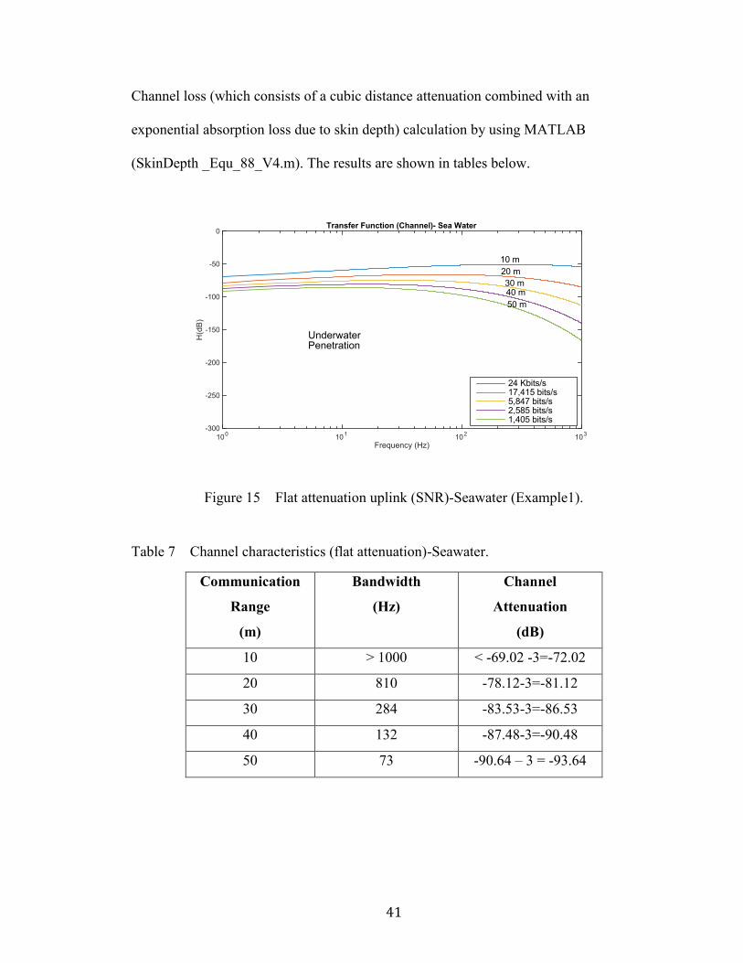
Channel loss (which consists of a cubic distance attenuation combined with an

exponential absorption loss due to skin depth) calculation by using MATLAB

(SkinDepth _Equ_88_V4.m). The results are shown in tables below.

Figure 15 Flat attenuation uplink (SNR)-Seawater (Example1).

Table 7 Channel characteristics (flat attenuation)-Seawater.

Communication

Range

(m)

Bandwidth

(Hz)

Channel

Attenuation

(dB)

10 > 1000 < -69.02 -3=-72.02

20 810 -78.12-3=-81.12

30 284 -83.53-3=-86.53

40 132 -87.48-3=-90.48

50 73 -90.64 – 3 = -93.64

Frequency (Hz)10

010

110

210

3

H(d

B)

-300

-250

-200

-150

-100

-50

0Transfer Function (Channel)- Sea Water

24 Kbits/s17,415 bits/s5,847 bits/s2,585 bits/s1,405 bits/s

20 m

50 m

30 m40 m

10 m

UnderwaterPenetration

42

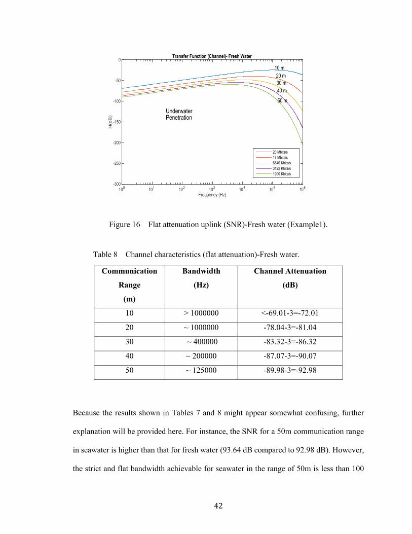
Figure 16 Flat attenuation uplink (SNR)-Fresh water (Example1).

Table 8 Channel characteristics (flat attenuation)-Fresh water.

Communication

Range

(m)

Bandwidth

(Hz)

Channel Attenuation

(dB)

10 > 1000000 <-69.01-3=-72.01

20 ~ 1000000 -78.04-3=-81.04

30 ~ 400000 -83.32-3=-86.32

40 ~ 200000 -87.07-3=-90.07

50 ~ 125000 -89.98-3=-92.98

Because the results shown in Tables 7 and 8 might appear somewhat confusing, further

explanation will be provided here. For instance, the SNR for a 50m communication range

in seawater is higher than that for fresh water (93.64 dB compared to 92.98 dB). However,

the strict and flat bandwidth achievable for seawater in the range of 50m is less than 100

Frequency (Hz)10

010

110

210

310

410

510

6

H(d

B)

-300

-250

-200

-150

-100

-50

0Transfer Function (Channel)- Fresh Water

20 Mbits/s

17 Mbits/s

6640 Kbits/s

3122 Kbits/s

1900 Kbits/s

10 m

20 m

30 m

40 m

UnderwaterPenetration

50 m

43

Hz, while this bandwidth exceeds 125 KHz in the case of fresh water. Thus, the quality of

communication differs significantly here.

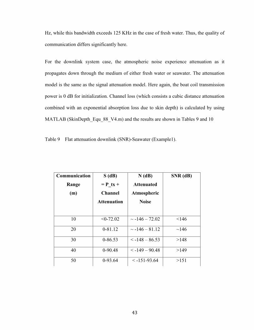
For the downlink system case, the atmospheric noise experience attenuation as it

propagates down through the medium of either fresh water or seawater. The attenuation

model is the same as the signal attenuation model. Here again, the boat coil transmission

power is 0 dB for initialization. Channel loss (which consists a cubic distance attenuation

combined with an exponential absorption loss due to skin depth) is calculated by using

MATLAB (SkinDepth_Equ_88_V4.m) and the results are shown in Tables 9 and 10

Table 9 Flat attenuation downlink (SNR)-Seawater (Example1).

Communication

Range

(m)

S (dB)

= P_tx +

Channel

Attenuation

N (dB)

Attenuated

Atmospheric

Noise

SNR (dB)

10 <0-72.02 ~ -146 – 72.02 <146

20 0-81.12 ~ -146 – 81.12 ~146

30 0-86.53 < -148 – 86.53 >148

40 0-90.48 < -149 – 90.48 >149

50 0-93.64 < -151-93.64 >151

44

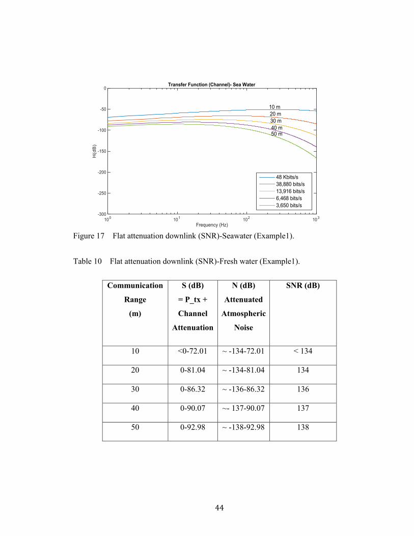
Figure 17 Flat attenuation downlink (SNR)-Seawater (Example1).

Table 10 Flat attenuation downlink (SNR)-Fresh water (Example1).

Frequency (Hz)10

010

110

210

3

H(d

B)

-300

-250

-200

-150

-100

-50

0Transfer Function (Channel)- Sea Water

48 Kbits/s

38,880 bits/s

13,916 bits/s

6,468 bits/s

3,650 bits/s

10 m

20 m

30 m

40 m50 m

Communication

Range

(m)

S (dB)

= P_tx +

Channel

Attenuation

N (dB)

Attenuated

Atmospheric

Noise

SNR (dB)

10

<0-72.01 ~ -134-72.01 < 134

20

0-81.04 ~ -134-81.04 134

30

0-86.32 ~ -136-86.32 136

40

0-90.07 ~- 137-90.07 137

50

0-92.98 ~ -138-92.98 138

45

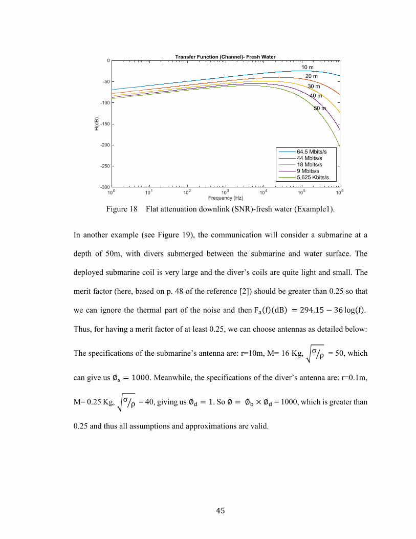
Figure 18 Flat attenuation downlink (SNR)-fresh water (Example1).

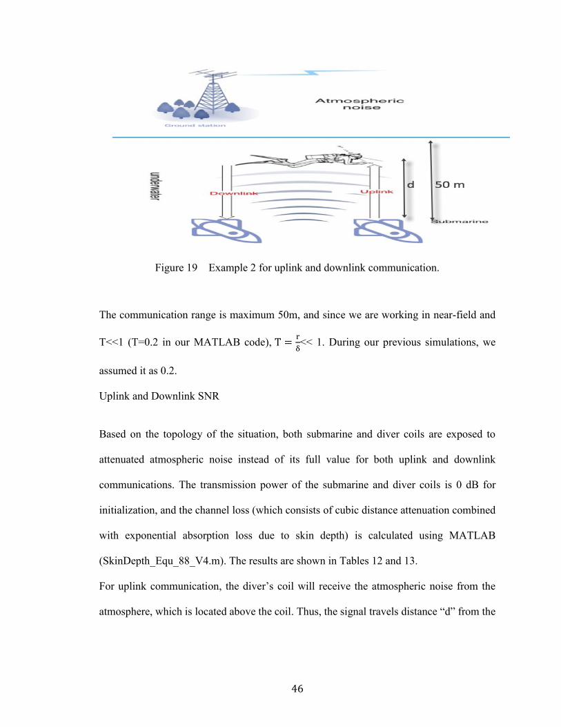
In another example (see Figure 19), the communication will consider a submarine at a

depth of 50m, with divers submerged between the submarine and water surface. The

deployed submarine coil is very large and the diver’s coils are quite light and small. The

merit factor (here, based on p. 48 of the reference [2]) should be greater than 0.25 so that

we can ignore the thermal part of the noise and then Fa(f)(dB) = 294.15 − 36 log(f).

Thus, for having a merit factor of at least 0.25, we can choose antennas as detailed below:

The specifications of the submarine’s antenna are: r=10m, M= 16 Kg, √σρ⁄ = 50, which

can give us ∅s = 1000. Meanwhile, the specifications of the diver’s antenna are: r=0.1m,

M= 0.25 Kg, √σρ⁄ = 40, giving us ∅d = 1. So ∅ = ∅b × ∅d = 1000, which is greater than

0.25 and thus all assumptions and approximations are valid.

Frequency (Hz)10

010

110

210

310

410

510

6

H(d

B)

-300

-250

-200

-150

-100

-50

0Transfer Function (Channel)- Fresh Water

64.5 Mbits/s44 Mbits/s18 Mbits/s9 Mbits/s5,625 Kbits/s

10 m

20 m

30 m

40 m

50 m

46

Figure 19 Example 2 for uplink and downlink communication.

The communication range is maximum 50m, and since we are working in near-field and

T<<1 (T=0.2 in our MATLAB code), T =r

δ<< 1. During our previous simulations, we

assumed it as 0.2.

Uplink and Downlink SNR

Based on the topology of the situation, both submarine and diver coils are exposed to

attenuated atmospheric noise instead of its full value for both uplink and downlink

communications. The transmission power of the submarine and diver coils is 0 dB for

initialization, and the channel loss (which consists of cubic distance attenuation combined

with exponential absorption loss due to skin depth) is calculated using MATLAB

(SkinDepth_Equ_88_V4.m). The results are shown in Tables 12 and 13.

For uplink communication, the diver’s coil will receive the atmospheric noise from the

atmosphere, which is located above the coil. Thus, the signal travels distance “d” from the

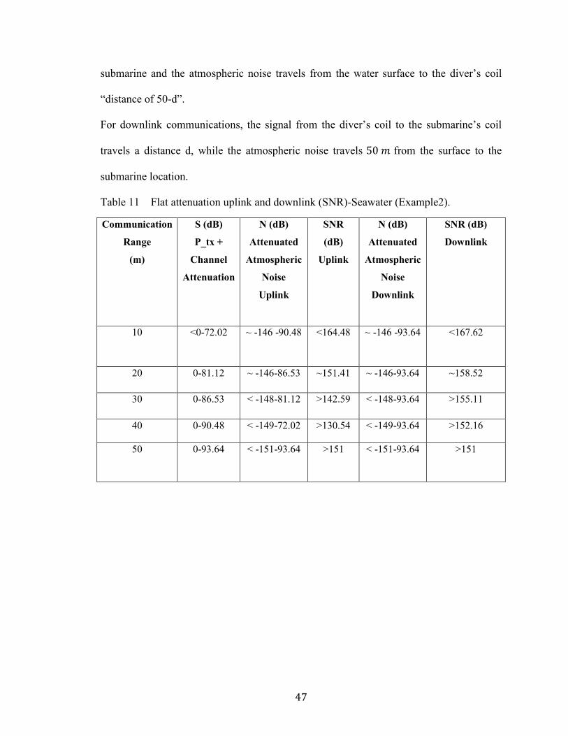
47

submarine and the atmospheric noise travels from the water surface to the diver’s coil

“distance of 50-d”.

For downlink communications, the signal from the diver’s coil to the submarine’s coil

travels a distance d, while the atmospheric noise travels 50 𝑚 from the surface to the

submarine location.

Table 11 Flat attenuation uplink and downlink (SNR)-Seawater (Example2).

Communication

Range

(m)

S (dB)

P_tx +

Channel

Attenuation

N (dB)

Attenuated

Atmospheric

Noise

Uplink

SNR

(dB)

Uplink

N (dB)

Attenuated

Atmospheric

Noise

Downlink

SNR (dB)

Downlink

10 <0-72.02 ~ -146 -90.48 <164.48 ~ -146 -93.64 <167.62

20 0-81.12 ~ -146-86.53 ~151.41 ~ -146-93.64 ~158.52

30 0-86.53 < -148-81.12 >142.59 < -148-93.64 >155.11

40 0-90.48 < -149-72.02 >130.54 < -149-93.64 >152.16

50 0-93.64 < -151-93.64 >151 < -151-93.64 >151

48

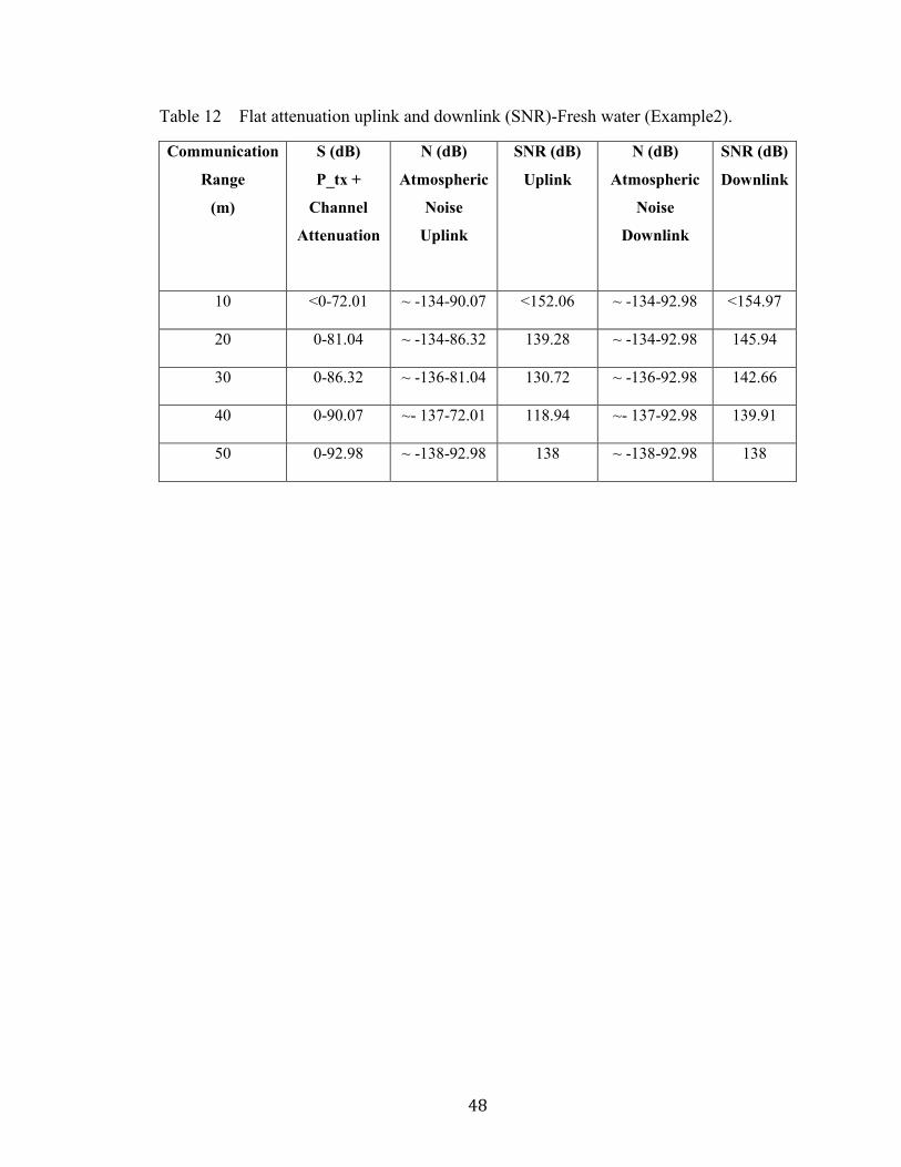
Table 12 Flat attenuation uplink and downlink (SNR)-Fresh water (Example2).

Communication

Range

(m)

S (dB)

P_tx +

Channel

Attenuation

N (dB)

Atmospheric

Noise

Uplink

SNR (dB)

Uplink

N (dB)

Atmospheric

Noise

Downlink

SNR (dB)

Downlink

10 <0-72.01 ~ -134-90.07 <152.06 ~ -134-92.98 <154.97

20 0-81.04 ~ -134-86.32 139.28 ~ -134-92.98 145.94

30 0-86.32 ~ -136-81.04 130.72 ~ -136-92.98 142.66

40 0-90.07 ~- 137-72.01 118.94 ~- 137-92.98 139.91

50 0-92.98 ~ -138-92.98 138 ~ -138-92.98 138

49

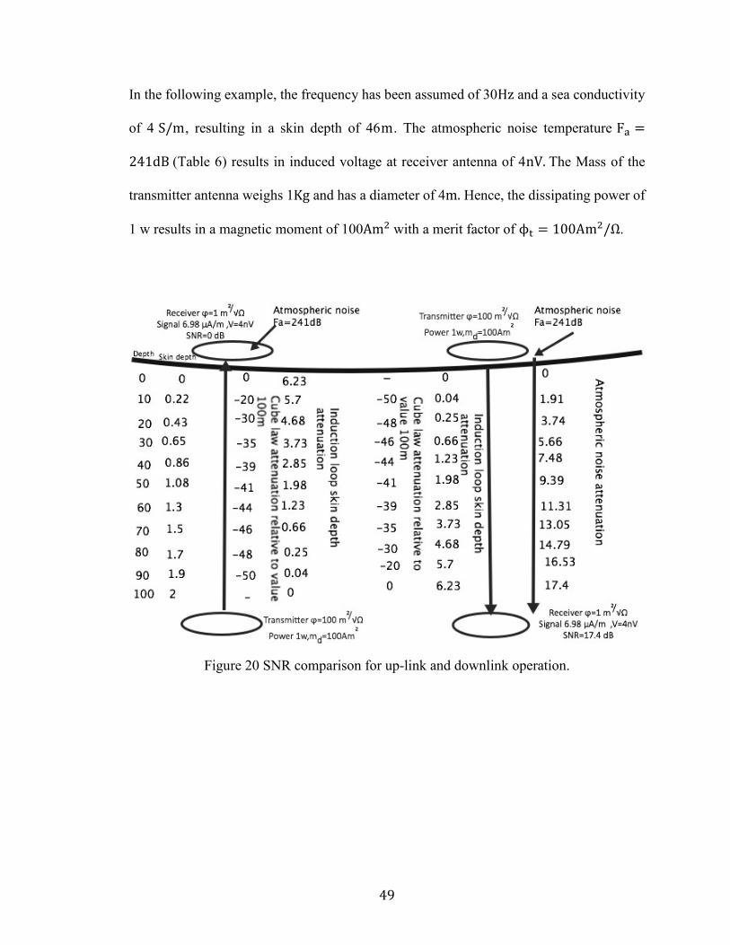
In the following example, the frequency has been assumed of 30Hz and a sea conductivity

of 4 S/m, resulting in a skin depth of 46m. The atmospheric noise temperature Fa =

241dB (Table 6) results in induced voltage at receiver antenna of 4nV. The Mass of the

transmitter antenna weighs 1Kg and has a diameter of 4m. Hence, the dissipating power of

1 w results in a magnetic moment of 100Am2 with a merit factor of ϕt = 100Am2/Ω.

Figure 20 SNR comparison for up-link and downlink operation.

50

1-Up-link Operation

In viewing Figure 20, which shows the SNR of 0 dB, we can assert that it is a convenient

value to describe the sensitivity of an antenna. However, despite its convenience, it is too

low to use in operations. Let us assume an operating distance of 50m (T = 1.08). The

signal strength will be 41 dB due to cube law attenuation and 1.98 dB instead of 6.23 due

to induction skin depth attenuation, resulting in SNR of 42.98 dB.

2- Down-link Operation

In downlink operations, the atmospheric noise is attenuated as 8.7 per skin depth. If we are

operating at 50m (T = 1.08), the SNR at the underwater receiver is increased by 9.39dB

due to atmospheric noise attenuation. Thus, we can conclude that we have a SNR of 52.37

dB at a range of 50m. If we want to keep the SNR at 42.98dB of up-link example, the

transmitter power must be reduced by 9.39dB or the underwater receiver antenna reduced

by 9.39dB (i.e., it must have a merit factor 2.9 times smaller).

51

CHAPTER5 CONCLUSION

This study examined the feasibility of improving communication under fresh and sea water

by way of a magneto-inductive (MI) communication method using a pair of coils as a

transmitter and receiver. In modeling the MI channel, both thermal and atmospheric noise

were studied and analyzed; however, under some certain circumstances and if the antenna’s

merit factor were greater than 0.25, the thermal noise could be ignored due to its

insignificance against atmospheric noise. The atmospheric noise by itself followed a

logarithmic equation that provided an approximate atmospheric noise-temperature ratio.

In terms of the communication field, the near-field region was the only one of interest in

the present dissertation. The near-field region covered all field points where the field

equations were described by quasi-static field formulas. It was also characterized by the

ratio of distance to skin depth, which had to be considerably less than 1. For the current

research and during the all MATLAB simulations, it was set to 0.2.

A cubic distance attenuation integrated with an exponential absorption loss was the channel

model used for the entire investigation. Its low pass characteristic was verified by

MATLAB simulations for both fresh and sea water, showing 0.01 and 4 S/m conductivities.

Thus, compared to sea water channel simulation results, fresh water offered a significantly

higher bandwidth communication channel. Consequently, better capacity was achievable

with the same transmission power. This indicates that the channel attenuation for sea water

was notably greater than the signal attenuation over a fresh water communication channel.

52

For example, to attain a distance of 100m, the channel bandwidth for fresh water was 25

KHz with an attenuation of -102.1 dB, whereas for sea water, these figures were degraded

to 10 Hz and -104.5 dB, respectively.

In terms of channel capacity, a better one is attainable for fresh water communication.

Thus, for communicating over a distance of 100m, a capacity of roughly 315.51 Kbps was

achievable for fresh water communication, whereas exchanging less than 200 bps was

possible for a sea water MI communication scheme.

In addition to channel transfer function modeling and its dependency on water

conductivity, transmission SNR proved to be another main factor for achieving a certain

range of effective communication, bandwidth, and channel capacity. However, it is worth

noting that a higher SNR can achieve longer communication distances with better

bandwidth and channel capacity. Moreover, the received SNR might be different at each

side of the MI communication. In other words, when the receiver antenna is at the water

surface, it is exposed to a broad range of atmospheric noise. The atmospheric noise then

experiences the channel attenuation for the receiving antenna that is under water. Thus, the

receiving antenna on the surface collects an attenuated transmitted signal as well as all the

atmospheric noise.

However, the SNR for the receiver antenna immersed in water is different, as it detects the

attenuated transmitted signal and atmospheric noise coming from the surface downward

towards the antenna cross-section. In the latter case, the received noise power is smaller

than the former situation, and if communication parties radiate the same transmission

53

power, its SNR will be higher. The mentioned situation has been demonstrated here by

detailed examples and has also been supported by MATLAB simulations.

Future work will focus on the optimization of the proposed and existing systems. Firstly,

Gibson showed that an optimal range does exist and that it features minimum channel

attenuation between transmitter and receiver. He also derived the T for triaxial and co-

planer coils, which is 2.83 and 3.85, respectively, and recommended using those T values

as alternative conditions for near-field MI schemes to achieve better results. Secondly,

during the course of existing research, the permittivity is assumed to be constant, whereas

the reality is that it is variable as well as frequency-, temperature-, and salinity-dependent.

Thus, trying to figure out its dependency and introduce the existing model with derived

results might give better results in future investigations. Thirdly, different antenna patterns

could be modelled and introduced to existing simulations so that the effects of different

shapes and designs could be studied in greater detail. Finally, The MI noise analysis and

measurements roughly match up, which means that theoretical equations can be used for

noise calculations. However, to obtain more accurate results, pre-amplifier noise could be

measured with newer and more precise techniques and then added to noise analysis

methods.

54

BIBLIOGRAPHY

[1] B. Gulbahar and O. B. Akan. A communication theoretical modeling and analysis of

underwater magneto-inductive wireless channels. IEEE Transactions on Wireless

Communications 11(9), pp. 3326-3334. 2012. . DOI:

10.1109/TWC.2012.070912.111943.

[2] C. Schlegel, M. Mallay and C. Touesnard. Atmospheric magnetic noise measurements

in urban areas. IEEE Magnetics Letters 5pp. 1-4. 2014. . DOI:

10.1109/LMAG.2014.2330337.

[3] A. D. W. Gibson, "Channel Characterisation and System Design for Sub Surface

Communications ." , University of Leeds, 2003.

[4] J. I. Agbinya. Principles of Inductive Near Field Communications for Internet of

Things, River Publishers, Denmark, 2011, ISBN: 978-87-92329-52-3.

[5] J. I. Agbinya and M. Masihpour. Near field magnetic induction communication link

budget: Agbinya-masihpour model. Presented at 2010 Fifth International Conference on

Broadband and Biomedical Communications. 2010, . DOI:

10.1109/IB2COM.2010.5723604.

[6] J. J. Sojdehei, P. N. Wrathall and D. F. Dinn. Magneto-inductive (MI)

communications. Presented at MTS/IEEE Oceans 2001. an Ocean Odyssey. Conference

Proceedings (IEEE Cat. no.01CH37295). 2001, . DOI: 10.1109/OCEANS.2001.968775.

[7] L. Erdogan and J. F. Bousquet. Dynamic bandwidth extension of coil for underwater

magneto-inductive communication. Presented at 2014 IEEE Antennas and Propagation

Society International Symposium (APSURSI). 2014, . DOI: 10.1109/APS.2014.6905114.

[8] M. C. Domingo. Magnetic induction for underwater wireless communication

networks. IEEE Transactions on Antennas and Propagation 60(6), pp. 2929-2939. 2012.

. DOI: 10.1109/TAP.2012.2194670.

[9] S. C. Lin et al. Distributed cross-layer protocol design for magnetic induction

communication in wireless underground sensor networks. IEEE Transactions on Wireless

Communications 14(7), pp. 4006-4019. 2015. . DOI: 10.1109/TWC.2015.2415812.

[10] S. Kisseleff, I. F. Akyildiz and W. H. Gerstacker. Throughput of the magnetic

induction based wireless underground sensor networks: Key optimization techniques.

IEEE Transactions on Communications 62(12), pp. 4426-4439. 2014. . DOI:

10.1109/TCOMM.2014.2367030.

55

[11] Seongwon Han et al. Evaluation of underwater optical-acoustic hybrid network.

China Communications 11(5), pp. 49-59. 2014. . DOI: 10.1109/CC.2014.6880460.

[12] T. E. Abrudan et al. Impact of rocks and minerals on underground magneto-

inductive communication and localization. IEEE Access 4pp. 3999-4010. 2016. . DOI:

10.1109/ACCESS.2016.2597641.

[13] X. Tan, Z. Sun and I. F. Akyildiz. Wireless underground sensor networks: MI-based

communication systems for underground applications. IEEE Antennas and Propagation

Magazine 57(4), pp. 74-87. 2015. . DOI: 10.1109/MAP.2015.2453917.

[14] Z. Sun and I. F. Akyildiz. Magnetic induction communications for wireless

underground sensor networks. IEEE Transactions on Antennas and Propagation 58(7),

pp. 2426-2435. 2010. . DOI: 10.1109/TAP.2010.2048858.