Underwater Inspection using Sonar-based Volumetric Submaps

Pedro V. Teixeira∗, Michael Kaess†, Franz S. Hover∗, and John J. Leonard∗

Abstract— We propose a submap-based technique for map-ping of underwater structures with complex geometries. Ourapproach relies on the use of probabilistic volumetric techniquesto create submaps from multibeam sonar scans, as these offerincreased outlier robustness. Special attention is paid to theproblem of denoising/enhancing sonar data. Pairwise submapalignment constraints are used in a factor graph frameworkto correct for navigation drift and improve map accuracy. Weprovide experimental results obtained from the inspection ofthe running gear and bulbous bow of a 600-foot, Wright-classsupply ship.

I. INTRODUCTION

Underwater mapping has a broad range of applications,including bathymetry, archaeological surveying, and the in-spection of complex underwater structures such as subseaequipment or ship hulls. As a result of the harsh environmen-tal conditions, mapping and inspection tasks are often per-formed by robots (either autonomous or remotely operated),equipped with optical and/or acoustic sensor payloads (e.g.cameras and sonars) typically capable of at least centimeterresolution. Still, the resolution of the resulting maps isusually lower, as the registration of sensor data is limitedby the uncertainty of the navigation solution. As it growsover time, this uncertainty quickly exceeds the resolutionof the sensors being used. While some applications—suchas bathymetric surveys of relatively open area—may allowthe use of absolute positioning systems that can limit thisgrowth (e.g. LBL or USBL), this is rarely the case whendealing with structures such as ship hulls; in such situations,the complex acoustic environment significantly impacts theoperation and performance of such systems due to effectssuch as multi-path or occultation.

Most of the sensors used in underwater mapping andinspection fall under the aforementioned categories—opticaland acoustic. Optical systems are of particular interest due totheir high resolution and low cost. Feature-based approachesfor optical imagery have been used to successfully navigateand map a ship’s hull [1]. Using features extracted fromstereo camera pair imagery, a “dense”1 smoothing techniqueis employed, allowing for tighter bounds to be placed onthe navigation uncertainty. One of the main disadvantages ofoptical systems, however, is their sensitivity to underwater

This work was partially supported by ONR grants N00014-12-1-0093and N00014-14-1-0373.∗Department of Mechanical Engineering, MIT, 77 Mas-

sachusetts Ave, Cambridge, MA 02139, USA {pvt, hover,jleonard}@mit.edu†Robotics Institute, Carnegie Mellon University, Pittsburgh, PA 15213,

USA kaess@cmu.edu1We use the term dense to refer to (smoothing) techniques where a new

pose is instantiated with every new measurement.

visibility conditions: with increased turbidity (common inharbors and near-shore environments), the range of opticalsensors decreases, negatively impacting their coverage rate,if not preventing their operation altogether. This limitationhas been addressed successfully in the context of shiphull inspection by utilizing an imaging sonar—again in afeature-based smoothing approach [2]. A common aspectto these techniques is that both target the smooth sectionsof the hull—the underlying assumption being that these aresufficiently smooth so that local planar approximations canbe made, onto which features can then be registered. Thisis not a limitation of either technique, but rather, of thesensor used (imaging sonars, for instance, have an inherentelevation ambiguity). Geometrically complex scenes, suchas a propeller, break this assumption and require us to useother sensors. While optical sensors are available that let uscircumvent this limitation, such as ranging lasers based oneither time-of-flight or structured light, they’re often verycostly and still subject to visibility issues, precluding theiruse in many man-made environments. Instead, their func-tionally equivalent acoustic counterparts, single- or multi-beam sonars, are often used for underwater mapping of morecomplex scenes.

Some of the earliest work on underwater mapping usedboth ship- and ROV-mounted multi-beam sonars to createbathymetric maps and inspect ship wrecks [3]. The sensormodel utilized took into consideration not only the finitewidth of a sonar beam, but also the uncertainty associatedwith the vehicle pose, making evidence grids especiallyattractive. More recently, a vehicle equipped with single-beam sonars was used to inspect and map flooded sinkholes[4]. The 2D SLAM technique used in that application relieson particle filters and a specialized occupancy grid imple-mentation that is amenable to the high number of operationsassociated with particle filter techniques.

Due to the nature of the measurements taken by thesesingle- and multi-beam sonars, the direct use of feature-based techniques (i.e. on individual measurements) is limited.Similar to side-scan sonars, multi-beam sonars return echointensities along rays cast from the sensor, in a plane normalto the vehicle’s trajectory (i.e. a grayscale image in polar co-ordinates), resulting in no overlap between subsequent mea-surements. This, together with the apparent lack of “feature-richness”, severely limits the use of “dense” techniquessuch as the ones previously mentioned. Submap techniquesaddress this limitation by accumulating measurements ina higher level map representation over some limited timeinterval.

Small ROVs equipped with mechanically swept sonars

2016 IEEE/RSJ International Conference on Intelligent Robots and Systems (IROS)Daejeon Convention CenterOctober 9-14, 2016, Daejeon, Korea

978-1-5090-3762-9/16/$31.00 ©2016 IEEE 4288

Fig. 1. Multibeam sonar: beam geometry (adapted from [2]).

have also been used to map man-made structures. Oneapproach has the ROV hover in place while the sonarassembles a full 360-degree, two-dimensional scan of itssurroundings, from which line features are extracted andutilized as landmarks in a filtering (EKF) context [5]. Alter-natively, scan-matching techniques can also be used to obtainrelative pose measurements [6]. This is of particular interestfor applications in less structured environments, such as theinspection of ancient water cisterns [7]. In this last example,a complete 2D map is built from pairwise registration ofscans. To mitigate the motion-induced errors associated withhovering, the ROV lands at the bottom of the cistern beforesweeping the sonar to assemble a scan.

Submap-based methods have also been successfully ap-plied to the problem of bathymetric mapping [8]. Regis-tered multi-beam returns are assembled into submaps, whichare checked for “richness” and consistency/drift. Like theprevious examples, pairwise submap registrations—obtainedthrough use of 2D correlation and Iterative Closest Point(ICP) algorithms—are incorporated in an EKF as relativepose measurements. A similar submap technique has alsobeen proposed in the context of ship hull inspection, re-placing filtering with smoothing by integrating pairwiseregistrations as loop-closure constraints in a factor graph [9].Finally, note that other submap techniques that deal with“dense” approaches are also available in the literature—see,for instance, Tectonic SAM [10], where submaps are createdby partitioning a pre-existing factor graph, and the Atlasframework [11], which aims at reducing computational effortby limiting the complexity of individual submaps.

The aim of this work is to develop a mapping techniqueable to produce a map of a complex underwater structurewith centimeter-level resolution. This resolution requirementstems from the features of interest in the ship hull inspectionscenario, which have characteristic dimensions on the orderof a few centimeters to a few tens of centimeters. Addition-ally, it is desirable that such a framework can be run in realtime, either due to the time-critical nature of some of shiphull inspection tasks, or so that the map can be used by anROV operator for navigation. Finally, our focus lies on map-building using only sonar data for sensing, for the reasonsmentioned above.

Our proposed approach builds upon previous work onsubmap-based mapping by combining the submap partition-ing techniques of [8] with a pose graph framework similar

to that of [9]. Moreover, we replace the direct registrationof sonar returns—common to both approaches—with theuse of volumetric techniques, preceded by enhancementand classification of sonar data. This increases robustnessto outliers and classification errors, reducing the need forsmoothing or filtering of submaps and improving the overallmap quality.

II. PROBLEM STATEMENT

The problem at hand, as previously mentioned, is that ofinspecting underwater structures with complex geometries(e.g. curved surfaces, non-convexities, sharp edges, etc.). Toaccomplish this task, we assume that a hovering AUV/ROVis used. These vehicles are typically equipped with the “stan-dard” navigation payload, comprising a Doppler VelocityLog (DVL), an Attitude and Heading Reference System(AHRS), and a depth sensor. By utilizing the attitude estimatefrom the AHRS, the DVL’s measurement of bottom-relativevelocity in body frame coordinates can be projected onto—and integrated in—the world frame. When combined withthe AHRS output, this constitutes a full 6DoF pose esti-mate; nevertheless, actual implementations will often replacethe z estimate obtained through integration with the directmeasurements available from high accuracy depth sensors.Furthermore, the use of tactical grade inertial measurementunits in the AHRS results in roll and pitch accuracies ofbetter than 0.1◦, reducing the pose estimation problem from6 to 3 degrees of freedom (x, y, and ψ). However, unlike theAHRS roll and pitch estimates, the yaw estimate is not drift-free. While this can be mitigated through the use of an aidingsensor such as a compass, this is not always desirable, par-ticularly when working in the proximity of metal structuressuch as a ship hull. As a result, the horizontal pose estimatesprovided by these systems are bound to drift over time. Asindicated in the previous section, inspection platforms oftencarry a multibeam sonar as part of its primary payload. Thesesonars comprise an array of transducers that produce one ormore narrow beams that sweep within a plane to create ascan (figure 1). The number of beams and their horizontal(i.e. “in-plane”) beam width determine the sonar’s horizontalfield of view2 and angular resolution. Range resolution isdetermined by the timing characteristics of the receivingcircuit (longer time bins will yield lower radial resolutionand vice versa). Typical values of a few hundred of beams,beam widths of 1◦ or less, centimeter-level range resolution,and typical ranges on the order of a few tens of meters makethem excellent sensors for underwater mapping, capable ofproviding high-resolution scans at large stand-off distances.Multi-beam sonars often output their measurements as a 2Darray, where each element corresponds to the return intensityfor that particular range and angle bin—essentially an imagein polar coordinates (see figure 3(a) for an example of asonar image after conversion to Cartesian coordinates).

Since our objective is to produce a map with a resolutionsuch that objects of a certain size can be identified, we

2With the vertical field of view being equal to the vertical width of abeam.

4289

Sonar Enhancement/denoising

Classification

SubmapperNavigation

Filter

SLAMSubmap catalog

Fig. 2. Overview of the proposed mapping pipeline.

must then ensure that the uncertainty associated with themapped sonar returns or features remains bounded and belowthe required resolution. This requires (i) robust classifica-tion/detection of valid sonar returns, (ii) accurate (short-term)registration of those returns, and (iii) long-term positionaccuracy through drift correction.

III. SUBMAP CREATION

Our submap creation pipeline can be summarized asfollows (figure 2): we begin by enhancing the incomingsonar data, with the aim of reducing some of the mostsignificant systematic errors present in the data. This makesrange extraction—the second step in our approach—muchmore reliable, seeing as there are less outliers in the data.Having extracted and registered the sonar ranges, they areinserted into an occupancy grid to build volumetric submaps,which are then converted into point clouds and filtered beforebeing handed over to the SLAM module (section IV).

A. Data Enhancement

Like any sensor, multibeam sonars are not free from eitherrandom or systematic error. Random error is caused both bythe acoustic noise in the environment and electronic noisein the transducer and signal processing circuitry. Systematicerror manifests itself in several different ways, and can betraced to a combination of causes, including non-zero beam-width, cross-talk, vehicle motion, and multi-path scattering[12]. Figure 3(a) shows a corner of a tank, as seen by themultibeam sonar used in our experiments (covered in greaterdetail in section V). There we observe both noise and theartifacts caused by the different error sources: angular andradial blur due to the non-zero beam-width; a mirror imageof one of the walls caused by multi-path scattering, andcrosstalk between transducer beams resulting in the curved(“arc”-like) feature. Considering that range extraction willrely on intensity values from the sonar scan, it is thus highlydesirable to mitigate these effects as much as possible.

Our approach to this problem is to model the sonar as alinear, time-invariant (LTI) system, where the output image yis the result of a convolution between the ideal image x andthe sonar impulse response h, under additive noise n(r, θ):

y(r, θ) = x(r, θ) ∗ h(r, θ) + n(r, θ) (1)

(a) (b)

Fig. 3. A sonar scan of a corner before (a) and after (b) enhancement.Sensor origin (not pictured) is located at the bottom the image, and rangeincreases towards the top.

If this model holds, we can then try to identify the sensorimpulse response (also known as point spread function, orPSF, in the context of imaging systems), and deconvolve theimage using a two-dimensional Wiener filter [13]. To modelthe PSF, however, we must first understand how the sonarforms an image.

To reduce cross-talk artifacts, the DIDSON fires its 96transducers in a staggered fashion—it takes 8 cycles, eachfiring 12 transducers, to form a complete image. This strategylimits cross-talk to the beams firing in the same cycle, which,despite being separated by 7 inactive transducers, are still“sensitive” to each other, as can be seen from figure 4.

If we assume the other transducers in the array havethe same beam pattern, then the PSF can be obtained bysampling the beam pattern at the angular positions of theother transducers firing in the same cycle. Note that thisapproach has some limitations in the sense that it (i) onlycaptures the angular component of the PSF, and, (ii) assumesthe PSF is isotropic. While addressing the former assumptionwould likely require some prior information about the scenebeing mapped, we can at least account for the angulardependence of the PSF by pre-multiplying the sonar imageby an angle-dependent function to account for the fact thatthe beam pattern for a transducer, while keeping the sameoverall shape, decreases in amplitude as we move awayfrom the center of the array. A similar approach is usedto compensate for the radial decay in return intensity, bymodeling both geometric and absorption losses. The resultsof this enhancement step are shown in figure 3.

B. Range extraction

Having enhanced the sonar image, the next step is toclassify it, that is, to detect the presence (or absence) ofobjects in the current scene. We follow a standard technique[5], [9], [14], [15] for multibeam sonar data by selecting, foreach beam, either the first or the strongest return that is abovea certain threshold. For the ith detected return, at coordinates(ri, θi), the 3D position of the return in the sonar frameis obtained by conversion to Cartesian coordinates: xs =[ri cos (θi), ri sin (θi), 0]T . Using homogeneous coordinates,

4290

Fig. 4. Typical beam pattern for one of the DIDSON’s beams—this willvary slightly over different sonars and lenses. (figure courtesy of SoundMetrics Corp., used with permission).

the location of that return in the global frame is

xg = T gv Tvs x

s (2)

where T vs is the (fixed) transform describing the sonar posein the vehicle frame, and T gv is the vehicle pose estimate inthe global frame, obtained from the navigation solution.

C. Volumetric mapping

Despite the improvements in return selection obtainedthrough the enhancement of sonar data, the classifier stillhas non-zero probabilities for both false positives (falsedetections) and false negatives (missed detections). This canbe further aggravated by the presence of bubbles, suspendedsediments, and fish schools, which, due to the strong sonarreturns they produce, will also be registered, effectivelyresulting in outliers. In order to mitigate the undesirableeffects of such outliers, we use probabilistic volumetrictechniques, where instead of registering returns, we updatethe occupancy probability for the region of space where thatreturn lies. These techniques have the additional advantagethat they let us use negative information—that is, we can usethe knowledge that the space between the vehicle and thereturn is empty to update the occupancy probability for theregions traversed by the beam. To compensate for the non-zero beam width and height of the sonar beams, we haveextended the OctoMap library [16] to support sonar beaminsertion—this allows us to implicitly model some of theangle uncertainty associated with a sonar return and, since alarger number of voxels have their occupancy probabilitiesupdated, obtain denser submaps.

D. Point clouds and filtering

Once a submap has been assembled, it is transformed to apoint cloud by thresholding: for each voxel whose occupancyprobability exceeds a user-defined level, a point is addedto the corresponding point cloud, with its coordinates beingequal to the center of the voxel. Since some outliers will stillmake their way through the volumetric submapping module,subsequent filtering is often necessary. For this purpose weemploy a clustering-based filter: points are first grouped

into clusters based on each point’s distance to their nearestneighbours(s), and small clusters (below a given number ofpoints) are then removed. The motivation for this filter stemsfrom the observation that these “persistent” outliers are, infact, the result of creatures and/or objects (e.g. fish, bubbles)that remain in the sonar’s field of view over the course of afew frames, leaving a small, sparse cloud of points in theirwake.

E. Submap span

On the one hand, submaps should be large enough soas to have enough geometric features that allow for asubmap to be registered against another; on the other, asubmap must be short enough that the accumulated odometryerror is small. Under linear motion at constant depth, andgiven measurement covariances of (σ2

x, σ2y) for the horizontal

velocity and σ2ψ for the yaw angle, the pose covariance after

Ti seconds is

Σi = Ti · diag(σ2x, σ

2y, σ

2ψ) (3)

The two main assumptions in the equation above—linearmotion and reduction to 3 dimensions—will be addressedin greater detail in the following sections.

IV. 3D SLAM

Using range measurements extracted from enhanced sonarscans, we have assembled a sequence of submaps connectedby odometry-based relative pose estimates. Knowing thatthese estimates are not drift-free, if we want to improvenavigation performance and map accuracy we must leveragethe information contained in the submaps. As we havepreviously mentioned, one way to do this is through pairwisesubmap registration: for any submap pair for which there isscene overlap, we can obtain a new relative pose constraintby aligning the two so that these match in the overlappingarea. While this can be a better estimate of relative pose,this is not always the case, especially for submaps with smalloverlap and/or simple geometries (e.g. mostly planar). As weobtain more of these estimates, we arrive at an optimizationproblem where we must try and find the pose estimates thatbest fit both odometry and pairwise registration constraints—we tackle this problem using a factor graph approach.

A. Factor graph

At every instant ti, a new pose estimate xi and sonar scanSi are available3. The relative pose between two subsequentscans can be written as:

ui,i+1 = xi+1 xi (4)

This can be represented as a factor graph, where eachpose estimate xi is associated with a node, and odometryconstraints ui,i+1 are represented as edges connecting thenodes for poses xi and xi+1. The assoicated covariance,Σi, can be determined using equation (3). At this point,

3Even though the sonar is likely not to output a new scan at the sametime or frequency as the navigation solution is computed, the latter can beinterpolated to obtain a pose estimate at the time a scan was received.

4291

the (acyclic) factor graph represents what is known as an“odometry chain” (figure 5), and the value of each pose canbe obtained through composition of odometry constraints.

B. Submapping in a factor graph perspective

In this factor graph representation, each node is implicitlypaired with the measurements taken at that instant—in ourcase, the sonar scans. For the reasons listed in section I, theseare rarely informative enough that loop closure informationcan be extracted from a pair of scans; instead, subsequentscans are “accumulated” into a finite set (represented bythe colors in figure 5(a)), so that constraints can then beobtained by pairwise analysis of these sets. This “accumu-lation” process—the assembly of volumetric submaps fromindividual sonar scans, introduced in section III-C—can bedescribed as the registration of all sonar scans in one submap,in the frame of the first pose of that submap: the basepose (figure 5(b)). The edges connecting the base poses ofsubmaps j and j + 1 are obtained by composition of theodometry constraints of the poses associated with submap j.

C. Pairwise registration

At this point we have arrived at a higher-level odometrychain, where each base node is associated with a submapinstead of a sonar scan (figure 5(c)); still, if navigationperformance is to be improved, additional constraints need tobe added to the factor graph. While detection and matchingof 3D features (such as planes) from submap pairs maybe a feasible technique, we intend to keep our techniquecapable of dealing with both structured and unstructuredenvironments—thus, we use scan matching to derive theseloop closure constraints.

Once a new submap is assembled, we begin by identifyingpotential matches by finding other submaps with which itoverlaps. For each potentially matching submap a transfor-mation estimate is computed through ICP [17], [18]. Sinceall points in each submap are referenced to its base pose,we compose the odometry constraints connecting the twonodes to arrive at the initial transformation estimate. Havingobtained a transformation estimate oij for the alignmentbetween submaps Si and Sj , we use the resulting score,as well as the time difference between submap acquisitions,to provide us with some guidance on its acceptance (e.g.the greater the time difference, the greater the threshold onthe difference between odometry and ICP transformations,as more drift is likely to have been accumulated). Givena process model xi = f(xi−1, ui−1) subject to additivewhite Gaussian noise (AWGN) wi with covariance, and ameasurement model ojk = h(xj , xk), also under AWGN vjk,we want to find the maximum a posteriori (MAP) estimateX = {x1, . . . , xN}:

XMAP = arg minX

( N∑i=1

‖f(xi−1, ui−1)− xi‖2

+∑

(j,k)∈O

‖h(xj , xk)− ojk‖2) (5)

px1 x2 x3 x4 x5 x6 x7

u12 u23 u34 u45 u56 u67

(a)

px1 x4 x7

u14 u47

(b)

px1 x4 x7

u14 u47

o47

(c)

Fig. 5. An overview of our submapping technique from a factor graphperspective: the starting graph (a) for the robot trajectory has each pose xi

connected to the next pose xi+1 by an edge ui,i+1 (odometry constraint)with associated covariance Σi; poses are grouped into submaps, withthe corresponding base poses replacing the originating poses (b); finally,pairwise constraints are added between base poses whose correspondingsubmaps have been co-registered (c). Note that the covariance matricesassociated with each edge are not represented.

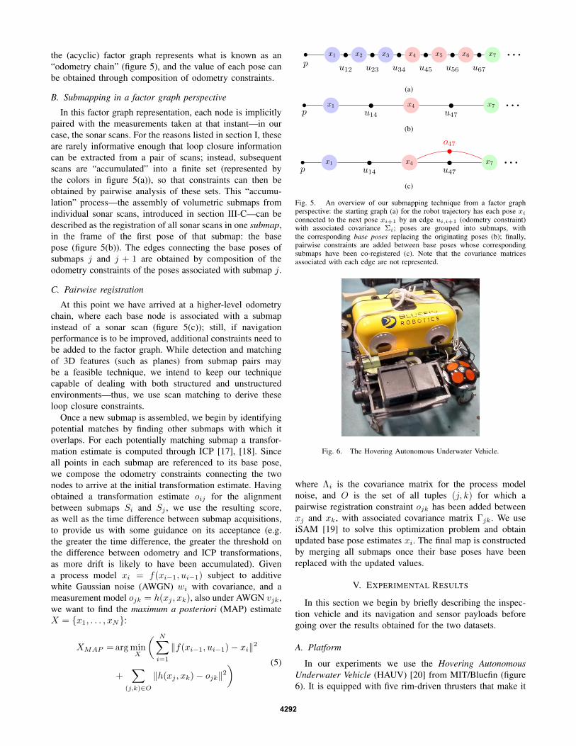
Fig. 6. The Hovering Autonomous Underwater Vehicle.

where Λi is the covariance matrix for the process modelnoise, and O is the set of all tuples (j, k) for which apairwise registration constraint ojk has been added betweenxj and xk, with associated covariance matrix Γjk. We useiSAM [19] to solve this optimization problem and obtainupdated base pose estimates xi. The final map is constructedby merging all submaps once their base poses have beenreplaced with the updated values.

V. EXPERIMENTAL RESULTS

In this section we begin by briefly describing the inspec-tion vehicle and its navigation and sensor payloads beforegoing over the results obtained for the two datasets.

A. Platform

In our experiments we use the Hovering AutonomousUnderwater Vehicle (HAUV) [20] from MIT/Bluefin (figure6). It is equipped with five rim-driven thrusters that make it

4292

TABLE INAVIGATION PAYLOAD: SENSOR PERFORMANCE

Sensor Axis Accuracy Unit

IMU Roll, Pitch 0.02 ◦

Yaw 0.05 ◦

DVL x,y,z 0.003 m/sDepth z 0.01 %

directly controllable in all axes but roll. Its navigation pay-load comprises a Honeywell HG1700 inertial measurementunit (IMU), a 1.2MHz Teledyne/RDI Workhorse NavigatorDVL, and a Paroscientific Digiquartz depth sensor—therelevant performance characteristics are summarized in tableI. The DVL can rotate parallel to the vehicle’s pitch axis,allowing for both bottom- and hull-relative motion.

The HAUV’s primary payload is a dual-frequency identi-fication sonar (DIDSON) [21], which we use primarily in itshigh frequency (1.8MHz) mode, as it provides greater detail.It has a total of 96 beams, each with 0.3◦ of horizontal beamwidth. Since we are interested in complex geometries, wemake use of a concentrator lens, reducing its vertical fieldof view from the standard 14◦ to 1◦ (-3dB values). Whileits range resolution depends on the minimum and maximumrange configuration, a typical window of 9.5 meters will yielda resolution of better than 2 centimeters.

B. SS Curtiss dataset

This dataset covers the inspection of the complex areasof the SS Curtiss: the running gear (rudder and propeller)and the bulbous bow (highlighted areas in figure 7). Bothdatasets were acquired while performing “coarse” surveys—essentially a vertical lawn-mower pattern (i.e. constant depthtransects) designed to rapidly create a map for the purposesof situational awareness. This is of particular use on un-seen ships or structures, before any close-in inspection isperformed. Since resolution is not as important as coverageand coverage rate, the vehicle is deployed with the sonar scanplane parallel to the hull’s longitudinal cross-section plane.Submap duration was chosen to be equal to 30 seconds,which, for the performance specifications listed in table I,corresponds to a horizontal uncertainty of approximately0.02m and 3◦ (1σ values). Finally, the results shown wereobtained in real time while performing inspection.

Fig. 7. Inspected regions of the hull of the SS Curtiss for the running gear(red) and bulbous bow (blue) datasets.

1) Running gear: This dataset comprises a “coarse” sur-vey of the running gear from the starboard side, covering therudder, propeller, and the hull sections immediately forwardof the latter. The coverage and results for this run are shownin figures 8(a) and 10, respectively.

By performing horizontal transects parallel to the ship’slongitudinal axis, we are able to quickly (approximately 30

(a)

(b)

Fig. 8. Submap coverage for the running gear (a) and bulbous bow(b) datasets (each colored patch represents a submap). The maps spanapproximately 45 and 39 meters, respectively. Map height is roughly equalto the ship’s draft: 9 meters.

minutes) cover one side of the running gear. However, therelatively fast coverage rate is not without disadvantages:the complex geometry of the propeller is poorly representedas the propeller is not imaged from its front or back,resulting in sparse coverage of each blade. Unlike the hulland rudder, which are nearly normal to the incident sonarbeams, propeller blades are ensonified at shallow angles,resulting in increased radial uncertainty in the sonar returns.

Despite the relatively short duration of this inspection run,there is still a significant amount of drift in the vehicle’shorizontal position estimates. This is especially evident onthe forward and aft edges of the map: the rudder appearsas multiple parallel sections (instead of a single, continuoussurface), with the distance between these sections reaching 2meters. The proposed SLAM technique is able to reduce thisworst-case distance to approximately 70cm while improvingthe overall shape of the map. This improvement is alsonoticeable towards the forward section of the map wherethis inter-submap distance is reduced from 1.2m to 40cm(approximate values).

2) Bulbous bow: A “coarse” survey of the bulbous bowof the ship, again from starboard side, was also performedand captured in this dataset. The coverage and results forthis run are shown in figures 8(b) and 11, respectively.

Like the previous dataset, inspection of the bow wasdone by performing horizontal transects parallel to the ship’slongitudinal axis. Due to the curvature of the hull, however,and in order to keep a consistent stand-off distance from thehull, a small yaw maneuver was performed about halfwaythrough each transect. This resulted in a rather large amountof drift, as can be seen from the forward and aft regionsof the map. On the top half of figure 11, it is possible todistinguish three “instances” of the bow tip—this has beensuccessfully corrected by the proposed SLAM technique(figure 11, bottom).

This inspection run also includes detailed inspection ofa test object placed on the hull prior to the inspection run,and found in the course of the survey. This results obtainedfrom a sample submap containing this object are shown infigure 9. From these we can see that while the shape hasnot been perfectly recovered (the object is a round metal

4293

(a)

(b)

(c)

Fig. 9. Submap with test object from the bulbous bow dataset: curvature-coded point clouds (profile (a) and perspective (b) views) and resultingmesh (c). Submap dimensions are approximately 1.3 by 5 meters; objectdimensions (as measured from the submap) are 11x32x22 centimeters.

cylinder 30cm in diameter), the submap is accurate enoughto represent features on the scale of a few centimeters. Alsoof note is the vertical gap in figures 9(a) and 9(b)—this isthe result of a missed sonar frame, possibly due to networkcongestion.

VI. CONCLUSION AND FUTURE WORK

We have proposed a technique for sonar-based SLAM that,while tailored to underwater scenes with complex geome-tries, can also be used in other applications such as bathy-metric mapping. This technique extends previous work byfocusing on improving submap accuracy through modelingof systematic errors and the use of probabilistic volumetrictechniques for increased outlier robustness. Experimentalvalidation on the problem of ship hull inspection indicatesthat it is both able to improve map accuracy by successfullycorrecting for navigation drift and represent features on theorder of a few centimeters.

In our approach to sonar data enhancement (section III),we limited modeling to the angular component of the pointspread function and made the assumption that it was angle-invariant. Relaxing these limitations should, in principle,yield better results: adding a radial dimension would improverange accuracy. Furthermore, the experimentally observedangular variation in beam pattern could be accounted for inan anisoplanatic PSF. Despite the relative success in elimi-nating outliers and improving overall submap quality, the useof volumetric techniques (as well as the subsequent filteringstep) points to the challenge of sonar image classification.Our classifier is biased towards “empty space” (instead ofoccupied) to reduce the number of outliers at the cost ofmissing actual returns—because of its simple threshold-based model, increasing its sensitivity would necessarily in-crease the number of outliers. Thus, improving classificationperformance is one of the main goals of ongoing work.

Still related to the classification problem, and motivated bythe end-use of the sonar in a mapping framework, is thepossibility of extracting additional information from sonardata, namely, surface orientation: given the narrow verticalfield of view of an imaging sonar, it should be possible to atleast restrict (if not completely determine) the orientation ofsurface elements to a finite set. This would be of particularuse to the registration (ICP) step in our SLAM approach,and to the reconstruction of a 3D mesh from the resultingset of maps—the data product of an inspection system.

Additional improvements to the accuracy of both theSLAM solution and final map could be obtained by delayingthe conversion from occupancy grids to point clouds tofurther along in the mapping pipeline. Replacing the use ofICP in the pairwise registration step with dense volumetricalignment techniques would improve pose estimate accuracyas both positive and negative information are used in theprocess. The final map could then be obtained by mergingthe different SLAM-corrected volumetric submaps onto asingle occupancy grid and only then reconstructing a pointcloud and/or 3D mesh. Finally, another relevant topic forfuture work would be the extension of these techniques tothe inspection of dynamic scenes.

REFERENCES

[1] P. Ozog and R. M. Eustice, “Real-time SLAM with piecewise-planarsurface models and sparse 3D point clouds,” in Int. Conf. IntelligentRobots and Syst. (IROS). IEEE, 2013, pp. 1042–1049.

[2] H. Johannsson, M. Kaess, B. Englot, F. Hover, and J. Leonard,“Imaging sonar-aided navigation for autonomous underwater harborsurveillance,” in Int. Conf. Intelligent Robots and Syst. (IROS). IEEE,2010, pp. 4396–4403.

[3] W. Stewart, “A non-deterministic approach to 3-D modeling under-water,” in Proc. 5th Int. Symp. Unmanned Untethered SubmersibleTechnology, vol. 5. IEEE, 1987, pp. 283–309.

[4] N. Fairfield, G. Kantor, D. Jonak, and D. Wettergreen, “Autonomousexploration and mapping of flooded sinkholes,” Int. J. of RoboticsResearch, vol. 29, no. 6, pp. 748–774, 2010.

[5] D. Ribas, P. Ridao, J. Neira, and J. D. Tardos, “SLAM using animaging sonar for partially structured underwater environments,” inInt. Conf. Intelligent Robots and Syst. (IROS). IEEE, 2006, pp. 5040–5045.

[6] A. Mallios, P. Ridao, D. Ribas, and E. Hernandez, “Probabilistic sonarscan matching SLAM for underwater environment,” in Oceans. IEEE,2010, pp. 1–8.

[7] W. McVicker, J. Forrester, T. Gambin, J. Lehr, Z. J. Wood, and C. M.Clark, “Mapping and visualizing ancient water storage systems withan ROV,” in Int. Conf. Robotics and Biomimetics (ROBIO). IEEE,2012, pp. 538–544.

[8] C. Roman and H. Singh, “A Self-Consistent Bathymetric MappingAlgorithm,” J. of Field Robotics, vol. 24, no. 1-2, pp. 23–50, 2007.

[9] M. VanMiddlesworth, M. Kaess, F. Hover, and J. Leonard, “Mapping3D Underwater Environments with Smoothed Submaps,” Brisbane,Australia, Dec. 2013.

[10] K. Ni, D. Steedly, and F. Dellaert, “Tectonic SAM: Exact, Out-of-Core, Submap-based SLAM,” in Int. Conf. Robotics and Automation(ICRA). IEEE, 2007, pp. 1678–1685.

[11] M. Bosse, P. Newman, J. Leonard, and S. Teller, “Simultaneouslocalization and map building in large-scale cyclic environments usingthe Atlas framework,” Int. J. of Robotics Research, vol. 23, no. 12,pp. 1113–1139, 2004.

[12] M. VanMiddlesworth, “Toward autonomous underwater mapping inpartially structured 3D environments,” Master’s thesis, MassachusettsInstitute of Technology, Feb. 2014.

[13] E. E. Hundt and E. A. Trautenberg, “Digital processing of ultrasonicdata by deconvolution,” Trans. on Sonics and Ultrasonics, vol. 27,no. 5, pp. 249–252, 1980.

4294

Fig. 10. Top view of the map of the running gear with depth-based color coding: odometry (top) and SLAM (bottom). This map was obtained throughconstant depth transects, with the vehicle running parallel to the ship’s longitudinal axis, and spans approximately 45 meters.

Fig. 11. Top view of the map of the bulbous bow with depth-based color coding: odometry (top) and SLAM (bottom). This map was obtained throughconstant depth transects, with the vehicle running parallel to the ship’s longitudinal axis and performing a yaw maneuver approximately halfway throughthe transect. The map spans approximately 39 meters.

[14] C. Roman and H. Singh, “Improved vehicle based multibeambathymetry using sub-maps and SLAM,” in Int. Conf. IntelligentRobots and Syst. (IROS). IEEE, 2005, pp. 3662–3669.

[15] A. Burguera, G. Oliver, and Y. Gonzalez, “Range extraction fromunderwater imaging sonar data,” in Int. Conf. Emerging Technologiesand Factory Automation (ETFA). IEEE, 2010, pp. 1–4.

[16] A. Hornung, K. M. Wurm, M. Bennewitz, C. Stachniss, andW. Burgard, “OctoMap: An efficient probabilistic 3D mappingframework based on octrees,” Autonomous Robots, 2013. [Online].Available: http://octomap.github.com

[17] P. J. Besl and N. D. McKay, “Method for Registration of 3-D Shapes,”in Robotics-DL tentative. Int. Society for Optics and Photonics, 1992,pp. 586–606.

[18] R. B. Rusu and S. Cousins, “3D is here: Point Cloud Pibrary (PCL),”in Int. Conf. Robotics and Automation (ICRA). IEEE, 2011, pp. 1–4.

[19] M. Kaess, A. Ranganathan, and F. Dellaert, “iSAM: IncrementalSmoothing and Mapping,” Trans. on Robotics, vol. 24, no. 6, pp.1365–1378, 2008.

[20] F. Hover, J. Vaganay, M. Elkins, S. Willcox, V. Polidoro, J. Morash,R. Damus, and S. Desset, “A vehicle system for autonomous relativesurvey of in-water ships,” Marine Technology Society J., vol. 41, no. 2,pp. 44–55, 2007.

[21] E. Belcher, W. Hanot, and J. Burch, “Dual-frequency identificationsonar (DIDSON),” in Proc. Int. Symp. Underwater Technology. IEEE,2002, pp. 187–192.

4295