Underwater Measurements of Pile-driving Sounds … Measurements of Pile Driving Sounds during the Port MacKenzie Dock Modifications, 13–16 August 20041 By Susanna B. …

Underwater Measurements of Pile Driving Sounds during the Port MacKenzie Dock Modifications,

13–16 August 20041

By

Susanna B. Blackwell Greeneridge Sciences, Inc.

1411 Firestone Road, Goleta, CA 93117 831-685-2773 (phone & FAX); [email protected]

Edited by

LGL Alaska Research Associates, Inc.

1101 E. 76th Ave., Suite B., Anchorage, AK 99518 (907) 562-3339

In association with

HDR Alaska, Inc.

2525 C Street, Suite 305 Anchorage, AK 99503

For

Knik Arm Bridge and Toll Authority (KABATA)

550 West 5th Ave., Suite 1850 Anchorage, AK 99501

Department of Transportation and Public Facilities

P.O. Box 196900 Anchorage, AK 99519-6900

Federal Highway Administration

P.O. Box 21648 Juneau, AK 99802

Greeneridge Report 328-1

March 2005

1 Suggested format for citations: Blackwell, S.B. 2005. Underwater measurements of pile-driving sounds during the Port MacKenzie dock modifications, 13-16 August 2004. Rep. from Greeneridge Sciences, Inc., Goleta, CA, and LGL Alaska Research Associates, Inc., Anchorage, AK, in association with HDR Alaska, Inc., Anchorage, AK, for Knik Arm Bridge and Toll Authority, Anchorage, AK, Department of Transportation and Public Facilities, Anchorage, AK, and Federal Highway Administration, Juneau, AK. 33 p.

mailto:[email protected]

Pile Driving Measurements at Port MacKenzie, AK

2

EXECUTIVE SUMMARY During August 2004 Greeneridge Sciences, Inc. made underwater recordings of

vibratory and impact pile driving sounds during the Port MacKenzie dock modifications in Cook Inlet, Alaska. Two 36-in. (91 cm) steel pipes of length 150 feet (46 m) were driven 40–50 feet into the seabed. The objectives were to characterize these construction sounds in terms of their broadband and one-third octave band levels and to gather information on transmission loss by repeated measurements of the same source at different distances.

The main recorded variables for vibratory and impact pile driving are summarized in the Table below.

Vibratory pile driving levels were difficult to compare to other studies because of dissimilar recording conditions. Impact pile driving levels were comparable to those obtained in several other studies in which large steel pipes were driven. NOAA Fisheries has specified that cetaceans should not be exposed to pulsed sounds exceeding 180 dB re 1 µPa sound pressure level (SPL). The distances at which mean SPLs decreased below 180 dB were 250 m and 195 m (820 feet and 640 feet) for measurements obtained with the deep and shallow hydrophones, respectively. Using maximum levels instead of means yielded more conservative estimates of 650 m and 330 m (2133 feet and 1083 feet) for the deep and shallow hydrophones, respectively.

Deep hydrophone

(10 m or 33 feet)

Shallow hydrophone

(1.5 m or 5 feet)

Vibratory pile driving

Mean SPL (rms) at 56 m(1) 164 dB re 1 µPa 162 dB re 1 µPa

Sound propagation loss 22 dB/decade(2) 29 dB/decade(2)

Dominant frequency range 400–2500 Hz

Peaks or tones 15 Hz and multiples thereof

Impact pile driving

Mean SPL (rms) at 62 m(3) 189 dB re 1 µPa 190 dB re 1 µPa

Mean instantaneous peak pressure at 62 m(3) 206 dB re 1 µPa 204 dB re 1 µPa

Mean sound exposure level at 62 m(3) 178 dB re 1 µPa2 · s 180 dB re 1 µPa2 · s

Sound propagation loss 16–18 dB/decade(2) 21–23 dB/decade(2)

Dominant frequency range 100–2000 Hz

Peaks or tones 350–450 Hz (1) Average of several 8.5-sec samples (2) or dB/tenfold change in distance (3) Average of several individual pulses


3

INTRODUCTION The Knik Arm Bridge and Toll Authority (KABATA), an arm of the Alaska

Department of Transportation and Public Facilities, proposes to construct, own, operate, and maintain a crossing that will span the Knik Arm in Alaska. The proposed crossing would provide direct transportation access between the Municipality of Anchorage (just north of the Port of Anchorage seaport) and Port MacKenzie in the Matanuska-Susitna Borough. Currently the crossing is in the planning phase.

Pile driving could occur during construction of the Knik Arm Crossing. Pile driving in or near water is known to produce strong pulses of underwater sound (Richardson et al. 1995, Würsig et al. 2000). There is concern regarding the effects of these sounds on marine life, particularly the resident population of beluga whales (Delphinapterus leucas). Beluga whales are thought to be present in Knik Arm year-round, but at a density and temporal pattern that is unknown for much of the year. Aerial surveys over a number of years (Rugh et al. 2000) have shown that the whales use Knik Arm extensively in the summer. The winter use of Knik Arm by belugas has been demonstrated more recently with satellite-tracked whales (Ferrero et al. 20002). The Cook Inlet beluga population is recognized by the National Oceanic and Atmospheric Administration (NOAA) Fisheries (formerly National Marine Fisheries Service [NMFS]) as an independent stock (Angliss and Lodge 2003). During the last 25 years, the stock has seen a large (nearly 80%) decline. As a result, in 2000 NMFS designated the stock as depleted under the Marine Mammal Protection Act.

The goals of this study were to use underwater acoustic recordings of construction noise associated with the Port MacKenzie dock modification (specifically vibratory and impact pile driving of pipes) to determine the level of sounds expected during construction of the crossing. Specifically, we aimed (1) to report peak values, sound pressure levels (SPLs) and sound exposure levels (SELs) for impact pile driving pulses as received at a range of distances from the pipes; (2) to report SPLs for vibratory pile driving sounds as received at a range of distances from the pipes; and (3) to characterize the acoustic properties of these sounds in terms of spectral composition and propagation loss between the different recording stations.

METHODS

Field Recordings of Underwater Sounds

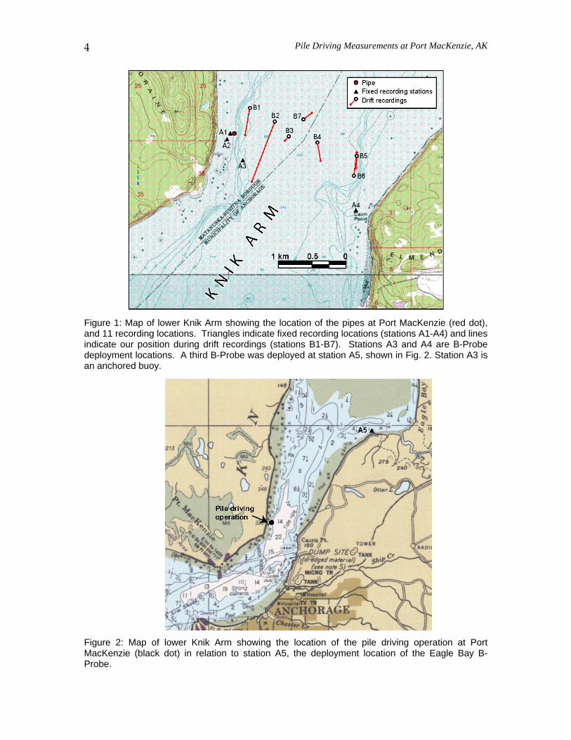
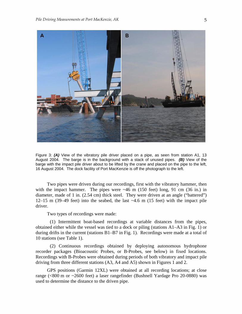
The position of the pipes was 61º 16.12’ N, 149º 54.91’ W. During the recordings, water depth around the pipes was tide-dependent, in the range 10–17 m (33–56 feet). The impact pile driver was a Delmag D62-22 with a 13.5-ton (12,280 kg) hammer and a maximum net impact energy of 223 kJ. The vibratory hammer was an APE (American Piledriving Equipment) model 400B (King Kong). Figures 1 and 2 show maps of lower Knik Arm with the locations of the recording stations (see below), and Figure 3 shows two views of the pile-driving operation at Port MacKenzie.

2 Also see data available at http://nmml.afsc.noaa.gov/ CetaceanAssessment/BelugaWhale.html

http://nmml.afsc.noaa.gov/ CetaceanAssessment/BelugaWhale.html


4

Figure 1: Map of lower Knik Arm showing the location of the pipes at Port MacKenzie (red dot), and 11 recording locations. Triangles indicate fixed recording locations (stations A1-A4) and lines indicate our position during drift recordings (stations B1-B7). Stations A3 and A4 are B-Probe deployment locations. A third B-Probe was deployed at station A5, shown in Fig. 2. Station A3 is an anchored buoy.

Figure 2: Map of lower Knik Arm showing the location of the pile driving operation at Port MacKenzie (black dot) in relation to station A5, the deployment location of the Eagle Bay B-Probe.


5

Figure 3: (A) View of the vibratory pile driver placed on a pipe, as seen from station A1, 13 August 2004. The barge is in the background with a stack of unused pipes. (B) View of the barge with the impact pile driver about to be lifted by the crane and placed on the pipe to the left, 16 August 2004. The dock facility of Port MacKenzie is off the photograph to the left.

Two pipes were driven during our recordings, first with the vibratory hammer, then with the impact hammer. The pipes were ~46 m (150 feet) long, 91 cm (36 in.) in diameter, made of 1 in. (2.54 cm) thick steel. They were driven at an angle (“battered”) 12–15 m (39–49 feet) into the seabed, the last ~4.6 m (15 feet) with the impact pile driver.

Two types of recordings were made:

(1) Intermittent boat-based recordings at variable distances from the pipes, obtained either while the vessel was tied to a dock or piling (stations A1–A3 in Fig. 1) or during drifts in the current (stations B1–B7 in Fig. 1). Recordings were made at a total of 10 stations (see Table 1).

(2) Continuous recordings obtained by deploying autonomous hydrophone recorder packages (Bioacoustic Probes, or B-Probes, see below) in fixed locations. Recordings with B-Probes were obtained during periods of both vibratory and impact pile driving from three different stations (A3, A4 and A5) shown in Figures 1 and 2.

GPS positions (Garmin 12XL) were obtained at all recording locations; at close range (<800 m or ~2600 feet) a laser rangefinder (Bushnell Yardage Pro 20-0880) was used to determine the distance to the driven pipe.


6

Boat-based recordings were made from a rigid-hulled inflatable boat. Two hydrophones were suspended directly from the vessel’s side into the water. Fairing was attached along the length of the hydrophone string to minimize strumming. The hydrophones were placed at depths of 10 m (33 feet) and 1.5 m (5 feet), unless water depth was shallower than 10.5 m (34 feet), in which case the deep hydrophone was placed 0.5–1 m (1.6–3.3 feet) above the bottom. Five-pound (2.3 kg) weights were attached next to each hydrophone to keep the hydrophone string as vertical as possible in the current. Tidal currents in Cook Inlet can be as high as 3.4 m/s (6.6 knots, Morsell et al. 1983). The boat’s engines and depth sounder were turned off during recordings.

A B-Probe was suspended by a faired line from an anchored buoy at Station A3. The depth was 2 m (6.6 feet) and the distance was ~370–400 m (1214–1312 feet) from the driven pipes (the range of distances is due to the buoy’s changing position with the tide). A 5 lb (2.3 kg) weight helped maintain vertical orientation. Water depth at the buoy was 29.5 m (97 feet) at high tide.

Another two B-Probes were anchored at Cairn Point (Station A4) and Eagle Bay (Station A5) as part of a study of the patterns of use of Knik Arm by beluga whales (see Funk et al. 2005). These B-Probes were used to evaluate the effectiveness of passive call detection to locate beluga whales near Cairn Point and the entrance to Eagle Bay. On August 27 the Cairn Point B-Probe (A4) recorded impact pile driving sounds from Port MacKenzie. On September 23 the Eagle Bay B-Probe (A5) recorded very weak impact pile driving sounds from Port MacKenzie. Both of these data sets were analyzed and are included in this report.

Background sound measurements were made opportunistically between pile driving sessions. However, the obtained values do not represent true “ambient” sound levels, as other sounds (such as vessel and industrial noise) were included on the recordings.

Acoustic Equipment

Boat-based Recordings The spherical hydrophones were International Transducer Corporation (ITC)

models 1032 at 10 m (33 feet) depth and 1042 at 1.5 m (5 feet) depth. Prior to recording the impact pile driving sounds, the sensitivity of these “barefoot” hydrophones was reduced with shunt capacitors (0.33 µF on each hydrophone). Gain was adjusted in 10-dB steps with an adjustable-gain preamplifier. Signals from both hydrophones were recorded simultaneously on two channels of a Sony model PC208Ax instrumentation-quality digital audiotape (DAT) recorder, at a sampling rate of 24 kHz. Quantization was 16 bits, providing a dynamic range of >80 dB between an overloaded signal and the quantization noise. Date and time were recorded automatically. The field acoustician noted the industry activities during each recording on a memo channel.

Bioacoustic Probe The Bioacoustic Probe, or B-Probe, is a self-contained acoustic data recorder

incorporating a calibrated hydrophone, a real-time clock, and a miniaturized digital recorder. The embedded hydrophone is a High-Tech, Inc. HTI-96-MIN/3V with internal preamplification. The B-Probes used in this experiment digitized signals from their


7

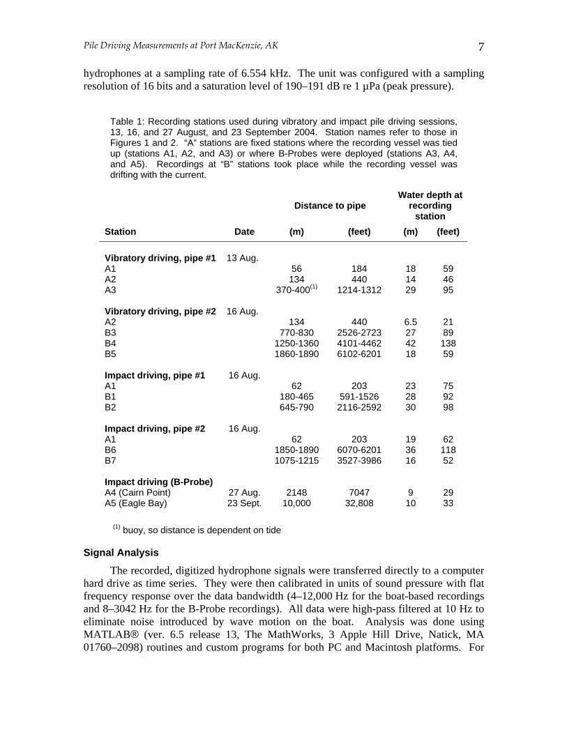
hydrophones at a sampling rate of 6.554 kHz. The unit was configured with a sampling resolution of 16 bits and a saturation level of 190–191 dB re 1 µPa (peak pressure).

Table 1: Recording stations used during vibratory and impact pile driving sessions, 13, 16, and 27 August, and 23 September 2004. Station names refer to those in Figures 1 and 2. “A” stations are fixed stations where the recording vessel was tied up (stations A1, A2, and A3) or where B-Probes were deployed (stations A3, A4, and A5). Recordings at “B” stations took place while the recording vessel was drifting with the current.

Distance to pipe Water depth at

recording station

Station Date (m) (feet) (m) (feet) Vibratory driving, pipe #1 A1 A2 A3 Vibratory driving, pipe #2 A2 B3 B4 B5 Impact driving, pipe #1 A1 B1 B2 Impact driving, pipe #2 A1 B6 B7 Impact driving (B-Probe) A4 (Cairn Point) A5 (Eagle Bay)

13 Aug.

16 Aug.

16 Aug.

16 Aug.

27 Aug. 23 Sept.

56 134

370-400(1)

134 770-830

1250-1360 1860-1890

62 180-465 645-790

62 1850-1890 1075-1215

2148

10,000

184 440

1214-1312

440 2526-2723 4101-4462 6102-6201

203 591-1526 2116-2592

203 6070-6201 3527-3986

7047 32,808

18 14 29

6.5 27 42 18

23 28 30

19 36 16

9 10

59 46 95

21 89

138 59

75 92 98

62 118 52

29 33

(1) buoy, so distance is dependent on tide

Signal Analysis

The recorded, digitized hydrophone signals were transferred directly to a computer hard drive as time series. They were then calibrated in units of sound pressure with flat frequency response over the data bandwidth (4–12,000 Hz for the boat-based recordings and 8–3042 Hz for the B-Probe recordings). All data were high-pass filtered at 10 Hz to eliminate noise introduced by wave motion on the boat. Analysis was done using MATLAB® (ver. 6.5 release 13, The MathWorks, 3 Apple Hill Drive, Natick, MA 01760–2098) routines and custom programs for both PC and Macintosh platforms. For


8

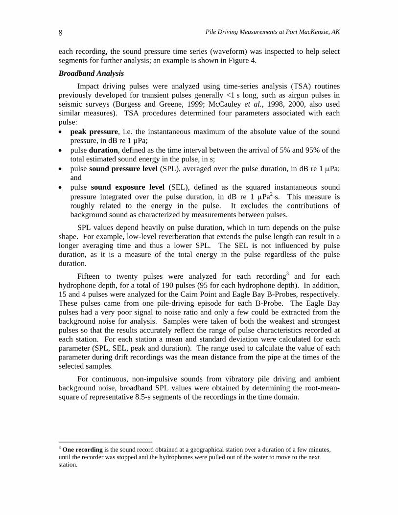
each recording, the sound pressure time series (waveform) was inspected to help select segments for further analysis; an example is shown in Figure 4.

Broadband Analysis Impact driving pulses were analyzed using time-series analysis (TSA) routines

previously developed for transient pulses generally <1 s long, such as airgun pulses in seismic surveys (Burgess and Greene, 1999; McCauley et al., 1998, 2000, also used similar measures). TSA procedures determined four parameters associated with each pulse: • peak pressure, i.e. the instantaneous maximum of the absolute value of the sound

pressure, in dB re 1 µPa; • pulse duration, defined as the time interval between the arrival of 5% and 95% of the

total estimated sound energy in the pulse, in s; • pulse sound pressure level (SPL), averaged over the pulse duration, in dB re 1 µPa;

and • pulse sound exposure level (SEL), defined as the squared instantaneous sound

pressure integrated over the pulse duration, in dB re 1 µPa2·s. This measure is roughly related to the energy in the pulse. It excludes the contributions of background sound as characterized by measurements between pulses.

SPL values depend heavily on pulse duration, which in turn depends on the pulse shape. For example, low-level reverberation that extends the pulse length can result in a longer averaging time and thus a lower SPL. The SEL is not influenced by pulse duration, as it is a measure of the total energy in the pulse regardless of the pulse duration.

Fifteen to twenty pulses were analyzed for each recording3 and for each hydrophone depth, for a total of 190 pulses (95 for each hydrophone depth). In addition, 15 and 4 pulses were analyzed for the Cairn Point and Eagle Bay B-Probes, respectively. These pulses came from one pile-driving episode for each B-Probe. The Eagle Bay pulses had a very poor signal to noise ratio and only a few could be extracted from the background noise for analysis. Samples were taken of both the weakest and strongest pulses so that the results accurately reflect the range of pulse characteristics recorded at each station. For each station a mean and standard deviation were calculated for each parameter (SPL, SEL, peak and duration). The range used to calculate the value of each parameter during drift recordings was the mean distance from the pipe at the times of the selected samples.

For continuous, non-impulsive sounds from vibratory pile driving and ambient background noise, broadband SPL values were obtained by determining the root-mean-square of representative 8.5-s segments of the recordings in the time domain.

3 One recording is the sound record obtained at a geographical station over a duration of a few minutes, until the recorder was stopped and the hydrophones were pulled out of the water to move to the next station.


9

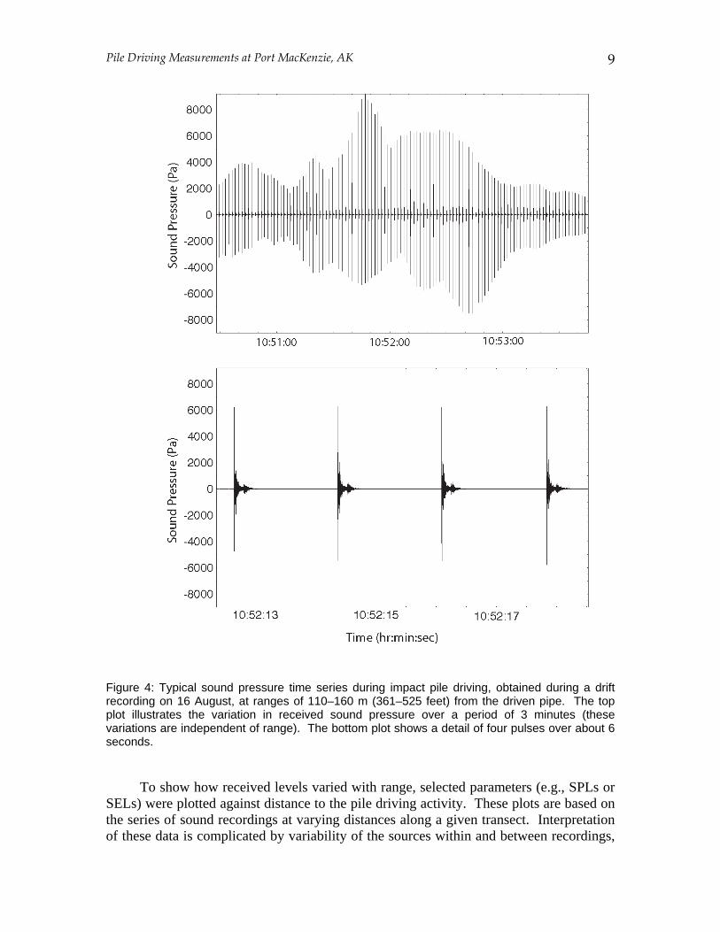
Figure 4: Typical sound pressure time series during impact pile driving, obtained during a drift recording on 16 August, at ranges of 110–160 m (361–525 feet) from the driven pipe. The top plot illustrates the variation in received sound pressure over a period of 3 minutes (these variations are independent of range). The bottom plot shows a detail of four pulses over about 6 seconds.

To show how received levels varied with range, selected parameters (e.g., SPLs or SELs) were plotted against distance to the pile driving activity. These plots are based on the series of sound recordings at varying distances along a given transect. Interpretation of these data is complicated by variability of the sources within and between recordings,


10

and by the likely contribution of sound from more than one sound source. Nevertheless, the “received level vs. distance” plots give an estimate of the range of levels received at several distances during the activity studied.

A simple propagation model was fitted by the least squares method to SPL, SEL and peak pressure values in order to characterize propagation loss underwater between different stations. The model was based on logarithmic spreading loss:

Received Level (RL) = A – B · log(R) (1)

In this equation, R is the distance from the source in m and the units for RL are dB re 1 µPa (for peak and SPL values) or 1 µPa2·s (for SEL values). The constant term (A) is the hypothetical extrapolated level 1 m from the source based on far-field measurements. This hypothetical value would equal the actual level at 1 m only if the source were a point source and if loss rates were consistent at all distances from 1 m to the maximum measurement distance, neither of which is the case. Therefore, the estimated A value is useful mainly as a basis for comparison with other sound sources operating in the same location. The spreading loss term (B) varies with the dominant frequency in the pulse, water depth, bottom topography and bottom composition. In deeper water, the depths of the source and receiver can also affect the value of B. Equation (1) is useful when there are few measured distances or when the greatest measurement range is short, less than 1 km. The model is generally not valid very far outside the range of distances used to compute the coefficients. When selecting data to include in deriving the model parameters, recordings were included at increasing distances from the sound source until the point at which levels reached a minimum and remained constant (within ~±2 dB). This technique avoided incorporation of weaker measurements dominated by ambient noise.

Spectral Analysis Spectral density levels were determined using Fourier transforms. (The Fourier

transform converts the time-domain characteristics of a sound into its frequency-domain characteristics.) For continuous sounds, spectral analysis was applied to a series of segments, overlapped by 50%, within a selected 8.5-s study interval. For transient impact pile driving pulses, spectral analysis was applied to a segment of sound containing a pulse and slightly longer than the pulse duration, typically a fraction of a second. Each segment was windowed and Fourier-transformed to obtain spectral density values for that segment. These spectral density values were then averaged across all segments in the selected interval. For the impact pile driving pulses, an interval of sound representing the background noise between the pulses was similarly analyzed and the results were subtracted from those of the pulse analysis to assure that the pulse spectra do not include background sound. The background spectra were retained for comparison with the pulse spectra.

For both continuous and impulsive sounds, one-third octave band levels over selected study intervals were calculated by performing a Fourier transform of the selected interval and integrating Fourier results between the band limits in the frequency domain.


11

A tone was defined when the sound pressure spectral density level (SPSDL) for a given frequency was greater than the SPSDL for both adjacent frequencies, and at least 5 dB above the nearest minimum SPSDL at a lower frequency.

RESULTS

Vibratory Pile Driving

Two sessions of vibratory pile driving were recorded, one on each of two pipes. The first occurred on 13 August and lasted about 20 min, 17:32–17:52 local time. High tide was at 19:00, so the tide was still coming in but was nearly at peak level. A second pipe was vibrated on 16 August for about 51 min, 15:21–16:12. This occurred right after low tide, which was at ~14:40. On both days the weather was fair, with partially clear skies and a sea state of 1 or less. The stations used during each driving session are listed in Table 1, together with water depth during the recordings. Maps of the lower Knik Arm and Port MacKenzie area with the recording locations are shown in Figures 1 and 2.

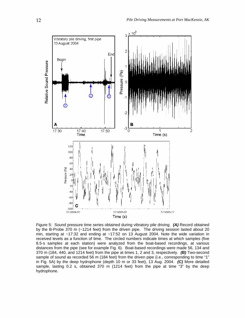
Broadband Sound Levels The B-Probe recorded sounds during vibratory driving of the first pipe on 13 Aug.,

from a distance of ~370 m (1214 feet). These data are presented in Figure 5A, showing sound pressure as a function of time for the period of interest. Data from the B-Probe show that sound levels were quite variable during the 20-min period of vibration. Figures 5B and 5C show 2-s and 0.2-s long sections of the sound pressure time series during vibratory pile driving. These examples were obtained with the deep hydrophone 56 m and 370 m (184 and 1214 feet), respectively, from the vibrated pipe.

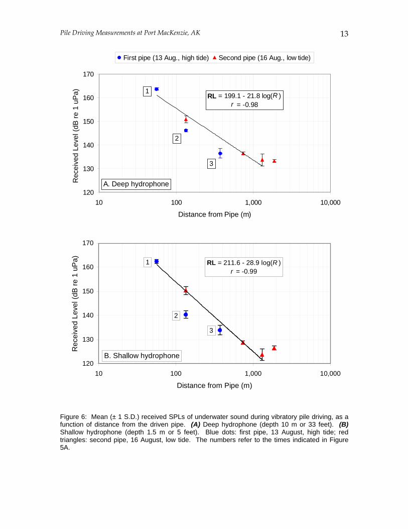
Mean received SPLs during vibratory driving, as received at all recording stations on both days (first pipe on 13 Aug. at high tide, second pipe on 16 Aug. at low tide), are shown in Figure 6A and 6B for the deep and shallow hydrophones, respectively. The highest recorded levels were obtained at station A1 (56 m or 184 feet from the source) and reached 164 dB re 1 µPa for both hydrophones.

The logarithmic sound propagation model [Eq. (1)] was fitted to received levels out to a distance of ~1300 m (4265 feet). For the 134 m (440 feet) station the higher level was used in the equation. The logarithmic coefficients [B in Eq. (1)] were 21.8 and 28.9 dB/tenfold change in distance for the deep and shallow hydrophones, respectively. Levels did not change significantly between the 1300 m (4265 feet) and 1900 m (6234 feet) stations, which suggests that beyond ~1300 m background sounds contributed more to received levels than vibratory pile driving did. The lower range of background levels, as recorded at the 370-m station while vibratory driving was not taking place, was 118 and 115 dB re 1 µPa for the deep and shallow hydrophones, respectively.


12

Figure 5: Sound pressure time series obtained during vibratory pile driving. (A) Record obtained by the B-Probe 370 m (~1214 feet) from the driven pipe. The driving session lasted about 20 min, starting at ~17:32 and ending at ~17:52 on 13 August 2004. Note the wide variation in received levels as a function of time. The circled numbers indicate times at which samples (five 8.5-s samples at each station) were analyzed from the boat-based recordings, at various distances from the pipe (see for example Fig. 6). Boat-based recordings were made 56, 134 and 370 m (184, 440, and 1214 feet) from the pipe at times 1, 2 and 3, respectively. (B) Two-second sample of sound as recorded 56 m (184 feet) from the driven pipe (i.e., corresponding to time “1” in Fig. 5A) by the deep hydrophone (depth 10 m or 33 feet), 13 Aug. 2004. (C) More detailed sample, lasting 0.2 s, obtained 370 m (1214 feet) from the pipe at time “3” by the deep hydrophone.


13

120

130

140

150

160

170

10 100 1,000 10,000

Distance from Pipe (m)

Rec

eive

d Le

vel (

dB re

1 u

Pa)

First pipe (13 Aug., high tide) Second pipe (16 Aug., low tide)

RL = 199.1 - 21.8 log(R )r = -0.98

1

2

3

A. Deep hydrophone

120

130

140

150

160

170

10 100 1,000 10,000


Rec

eive

d Le

vel (

dB re

1 u

Pa) RL = 211.6 - 28.9 log(R )

r = -0.99

B. Shallow hydrophone

2

1

3

Figure 6: Mean (± 1 S.D.) received SPLs of underwater sound during vibratory pile driving, as a function of distance from the driven pipe. (A) Deep hydrophone (depth 10 m or 33 feet). (B) Shallow hydrophone (depth 1.5 m or 5 feet). Blue dots: first pipe, 13 August, high tide; red triangles: second pipe, 16 August, low tide. The numbers refer to the times indicated in Figure 5A.


14

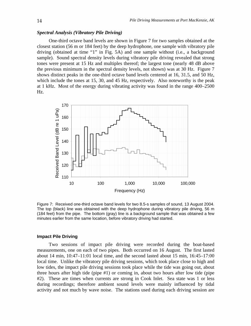
Spectral Analysis (Vibratory Pile Driving) One-third octave band levels are shown in Figure 7 for two samples obtained at the

closest station (56 m or 184 feet) by the deep hydrophone, one sample with vibratory pile driving (obtained at time “1” in Fig. 5A) and one sample without (i.e., a background sample). Sound spectral density levels during vibratory pile driving revealed that strong tones were present at 15 Hz and multiples thereof; the largest tone (nearly 48 dB above the previous minimum in the spectral density levels, not shown) was at 30 Hz. Figure 7 shows distinct peaks in the one-third octave band levels centered at 16, 31.5, and 50 Hz, which include the tones at 15, 30, and 45 Hz, respectively. Also noteworthy is the peak at 1 kHz. Most of the energy during vibrating activity was found in the range 400–2500 Hz.

110

120

130

140

150

160

170

10 100 1,000 10,000 100,000

Frequency (Hz)

Rec

eive

d B

and

Leve

l (dB

re 1

uP

a)

Figure 7: Received one-third octave band levels for two 8.5-s samples of sound, 13 August 2004. The top (black) line was obtained with the deep hydrophone during vibratory pile driving, 56 m (184 feet) from the pipe. The bottom (gray) line is a background sample that was obtained a few minutes earlier from the same location, before vibratory driving had started.

Impact Pile Driving

Two sessions of impact pile driving were recorded during the boat-based measurements, one on each of two pipes. Both occurred on 16 August. The first lasted about 14 min, 10:47–11:01 local time, and the second lasted about 15 min, 16:45–17:00 local time. Unlike the vibratory pile driving sessions, which took place close to high and low tides, the impact pile driving sessions took place while the tide was going out, about three hours after high tide (pipe #1) or coming in, about two hours after low tide (pipe #2). These are times when currents are strong in Cook Inlet. Sea state was 1 or less during recordings; therefore ambient sound levels were mainly influenced by tidal activity and not much by wave noise. The stations used during each driving session are


15

listed in Table 1, together with water depth during the recordings. Maps of the lower Knik Arm and Port MacKenzie area with the recording locations are shown in Figures 1 and 2.

A third session of impact pile driving was recorded by a B-Probe deployed at Cairn Point (station A4) as part of the beluga whale study in Knik Arm (see Funk et al. 2005). This session took place on 27 August from 17:44 to 18:04 local time, corresponding with high tide. The B-Probe was anchored to a concrete block near the bottom; water depth was ~9 m (30 feet) during the recorded pile driving session. Data analyzed from this recorder have been plotted with data from the deep hydrophone (see below).

The Eagle Bay B-Probe (station A5) recorded a fourth pile driving session on 23 September. The pile driving sounds were very weak and difficult to isolate from background and recorder noises. Four pulses were analyzed between 16:32 and 17:12 local time, i.e., about one hour after high tide. The B-Probe was anchored to a concrete block near the bottom; water depth was ~10 m (33 feet) during the analyzed pulses. A straight line drawn on Figure 2 between the pile driving site and the B-Probe location (station A5) crosses areas of mudflats and even some land. For that reason, it is not justified to include the results from the analyses of these pulses on the sound level vs. distance plots presented later. Values for SPL, SEL and pulse duration are instead presented in Table 2 for the Eagle Bay B-Probe. Peak values were impossible to determine accurately due to the pulses’ proximity to the lower detection limit of the recorder.

The B-Probe deployed at station A3 (range 370 m or 1214 feet, see Fig. 1) recorded data during the first pile driving session on 16 August but the hydrophone saturated because of peak levels above 191 dB re 1 µPa.

Table 2: Sound pressure level (SPL), sound exposure level (SEL), and pulse duration for the four pulses analyzed from the Eagle Bay B-Probe (station A4).

Pulse time SPL SEL Duration (dB re 1 µPa) (dB re 1 µPa2·s) (s)

16:32:32.5 16:40:36.4 16:48:11.5 17:12:46.5

94.0 94.6 95.1 98.0

90.7 91.0 91.9 94.0

0.47 0.43 0.48 0.41

Broadband Sound Levels Examples of sound pressure time series for impact pile driving sounds were

presented earlier in Figure 4. These examples were obtained from the recording vessel while drifting, 110–160 m (361–525 feet) from the pipe. Note the wide variation in sound pressure, independent of the distance to the pipe.


16

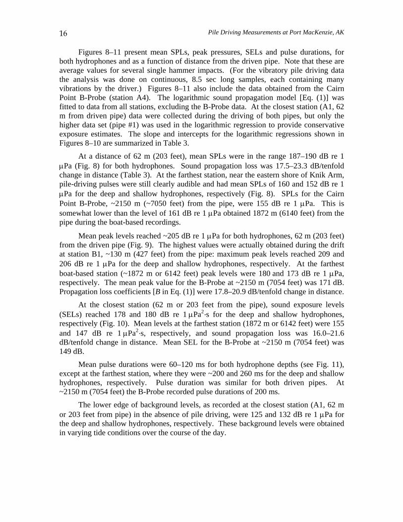
Figures 8–11 present mean SPLs, peak pressures, SELs and pulse durations, for both hydrophones and as a function of distance from the driven pipe. Note that these are average values for several single hammer impacts. (For the vibratory pile driving data the analysis was done on continuous, 8.5 sec long samples, each containing many vibrations by the driver.) Figures 8–11 also include the data obtained from the Cairn Point B-Probe (station A4). The logarithmic sound propagation model [Eq. (1)] was fitted to data from all stations, excluding the B-Probe data. At the closest station (A1, 62 m from driven pipe) data were collected during the driving of both pipes, but only the higher data set (pipe #1) was used in the logarithmic regression to provide conservative exposure estimates. The slope and intercepts for the logarithmic regressions shown in Figures 8–10 are summarized in Table 3.

At a distance of 62 m (203 feet), mean SPLs were in the range 187–190 dB re 1 µPa (Fig. 8) for both hydrophones. Sound propagation loss was 17.5–23.3 dB/tenfold change in distance (Table 3). At the farthest station, near the eastern shore of Knik Arm, pile-driving pulses were still clearly audible and had mean SPLs of 160 and 152 dB re 1 µPa for the deep and shallow hydrophones, respectively (Fig. 8). SPLs for the Cairn Point B-Probe, ~2150 m (~7050 feet) from the pipe, were 155 dB re 1 µPa. This is somewhat lower than the level of 161 dB re 1 µPa obtained 1872 m (6140 feet) from the pipe during the boat-based recordings.

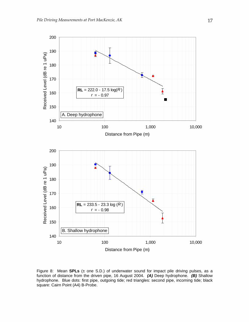
Mean peak levels reached ~205 dB re 1 µPa for both hydrophones, 62 m (203 feet) from the driven pipe (Fig. 9). The highest values were actually obtained during the drift at station B1, ~130 m (427 feet) from the pipe: maximum peak levels reached 209 and 206 dB re 1 µPa for the deep and shallow hydrophones, respectively. At the farthest boat-based station (~1872 m or 6142 feet) peak levels were 180 and 173 dB re 1 µPa, respectively. The mean peak value for the B-Probe at ~2150 m (7054 feet) was 171 dB. Propagation loss coefficients [B in Eq. (1)] were 17.8–20.9 dB/tenfold change in distance.

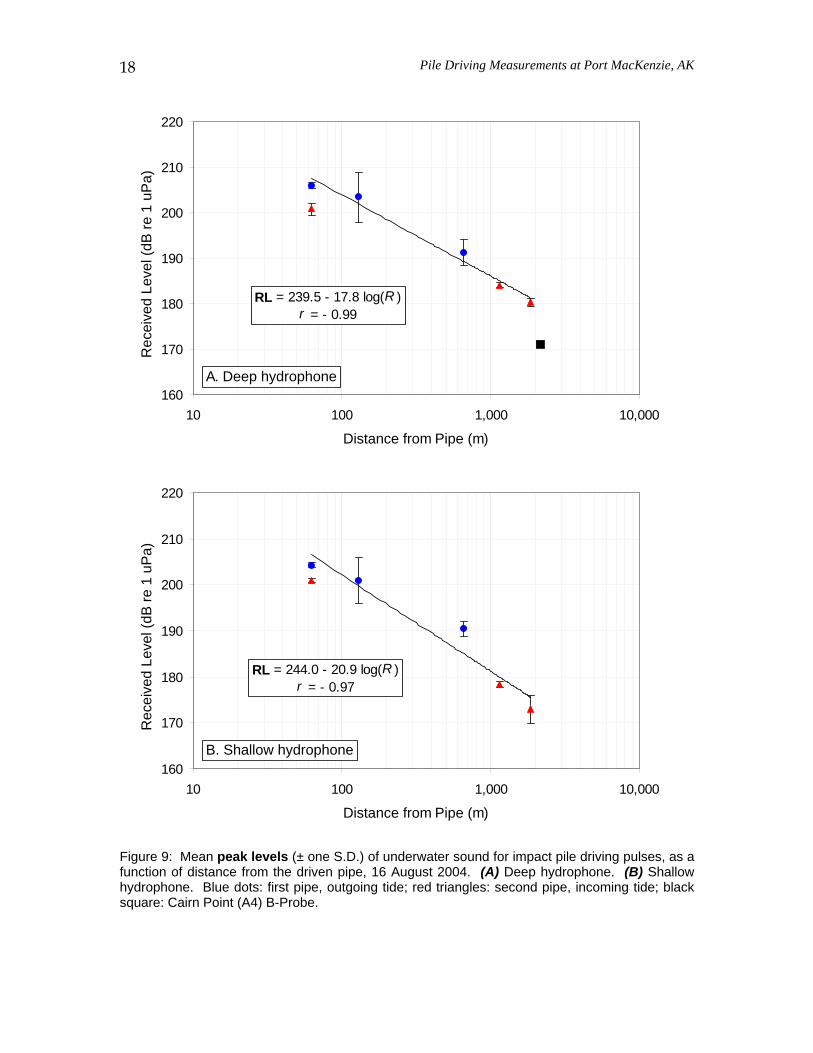
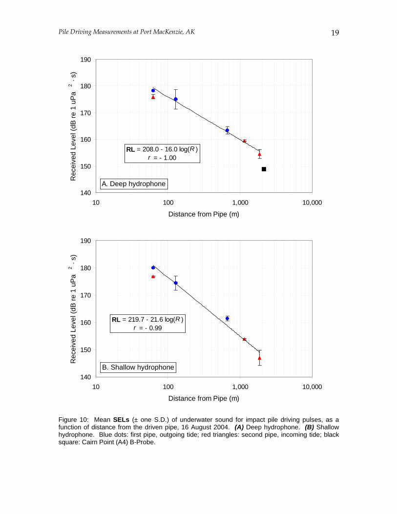
At the closest station (62 m or 203 feet from the pipe), sound exposure levels (SELs) reached 178 and 180 dB re 1 µPa2·s for the deep and shallow hydrophones, respectively (Fig. 10). Mean levels at the farthest station (1872 m or 6142 feet) were 155 and 147 dB re 1 µPa2·s, respectively, and sound propagation loss was 16.0–21.6 dB/tenfold change in distance. Mean SEL for the B-Probe at ~2150 m (7054 feet) was 149 dB.

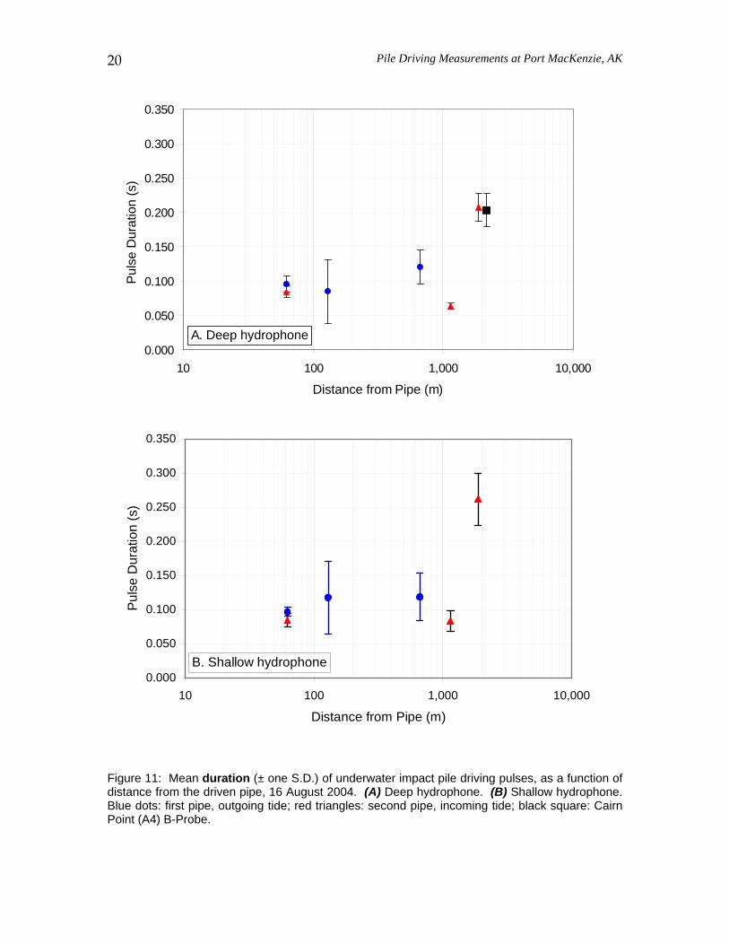
Mean pulse durations were 60–120 ms for both hydrophone depths (see Fig. 11), except at the farthest station, where they were ~200 and 260 ms for the deep and shallow hydrophones, respectively. Pulse duration was similar for both driven pipes. At ~2150 m (7054 feet) the B-Probe recorded pulse durations of 200 ms.

The lower edge of background levels, as recorded at the closest station (A1, 62 m or 203 feet from pipe) in the absence of pile driving, were 125 and 132 dB re 1 µPa for the deep and shallow hydrophones, respectively. These background levels were obtained in varying tide conditions over the course of the day.


17

140

150

160

170

180

190

200

10 100 1,000 10,000


Rec

eive

d Le

vel (

dB re

1 u

Pa)

A. Deep hydrophone

RL = 222.0 - 17.5 log(R )r = - 0.97

140

150

160

170

180

190

200

10 100 1,000 10,000


Rec

eive

d Le

vel (

dB re

1 u

Pa)


RL = 233.5 - 23.3 log (R )r = - 0.98

Figure 8: Mean SPLs (± one S.D.) of underwater sound for impact pile driving pulses, as a function of distance from the driven pipe, 16 August 2004. (A) Deep hydrophone. (B) Shallow hydrophone. Blue dots: first pipe, outgoing tide; red triangles: second pipe, incoming tide; black square: Cairn Point (A4) B-Probe.


18

160

170

180

190

200

210

220

10 100 1,000 10,000


Rec

eive

d Le

vel (

dB re

1 u

Pa)

A. Deep hydrophone

RL = 239.5 - 17.8 log(R )r = - 0.99

160

170

180

190

200

210

220

10 100 1,000 10,000


Rec

eive

d Le

vel (

dB re

1 u

Pa)


RL = 244.0 - 20.9 log(R )r = - 0.97

Figure 9: Mean peak levels (± one S.D.) of underwater sound for impact pile driving pulses, as a function of distance from the driven pipe, 16 August 2004. (A) Deep hydrophone. (B) Shallow hydrophone. Blue dots: first pipe, outgoing tide; red triangles: second pipe, incoming tide; black square: Cairn Point (A4) B-Probe.


19

140

150

160

170

180

190

10 100 1,000 10,000


Rec

eive

d Le

vel (

dB re

1 u

Pa

2 ·

s)

A. Deep hydrophone

RL = 208.0 - 16.0 log(R )r = - 1.00

140

150

160

170

180

190

10 100 1,000 10,000


Rec

eive

d Le

vel (

dB re

1 u

Pa

2 ·

s)


RL = 219.7 - 21.6 log(R )r = - 0.99

Figure 10: Mean SELs (± one S.D.) of underwater sound for impact pile driving pulses, as a function of distance from the driven pipe, 16 August 2004. (A) Deep hydrophone. (B) Shallow hydrophone. Blue dots: first pipe, outgoing tide; red triangles: second pipe, incoming tide; black square: Cairn Point (A4) B-Probe.


20

0.000

0.050

0.100

0.150

0.200

0.250

0.300

0.350

10 100 1,000 10,000


Pul

se D

urat

ion

(s)

A. Deep hydrophone

0.000

0.050

0.100

0.150

0.200

0.250

0.300

0.350

10 100 1,000 10,000


Pul

se D

urat

ion

(s)


Figure 11: Mean duration (± one S.D.) of underwater impact pile driving pulses, as a function of distance from the driven pipe, 16 August 2004. (A) Deep hydrophone. (B) Shallow hydrophone. Blue dots: first pipe, outgoing tide; red triangles: second pipe, incoming tide; black square: Cairn Point (A4) B-Probe.


21

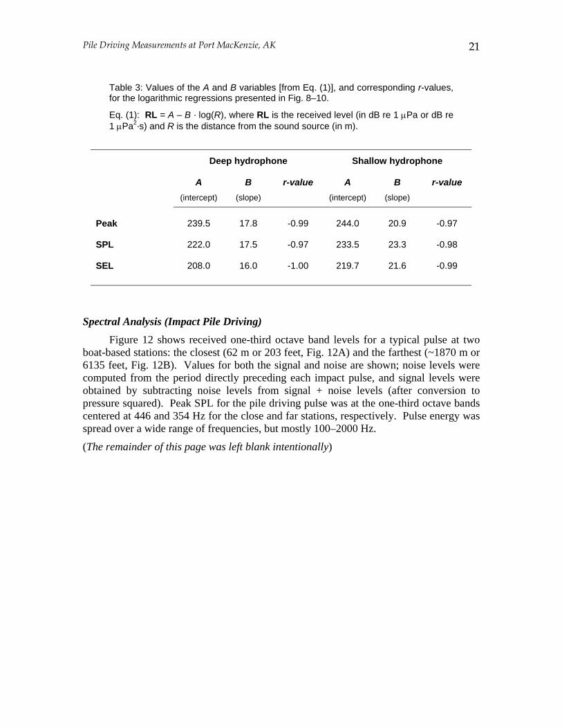
Table 3: Values of the A and B variables [from Eq. (1)], and corresponding r-values, for the logarithmic regressions presented in Fig. 8–10.

Eq. (1): RL = A – B · log(R), where RL is the received level (in dB re 1 µPa or dB re 1 µPa2·s) and R is the distance from the sound source (in m).

Deep hydrophone Shallow hydrophone

A (intercept)

B (slope)

r-value A (intercept)

B (slope)

r-value

Peak SPL SEL

239.5

222.0

208.0

17.8

17.5

16.0

-0.99

-0.97

-1.00

244.0

233.5

219.7

20.9

23.3

21.6

-0.97

-0.98

-0.99

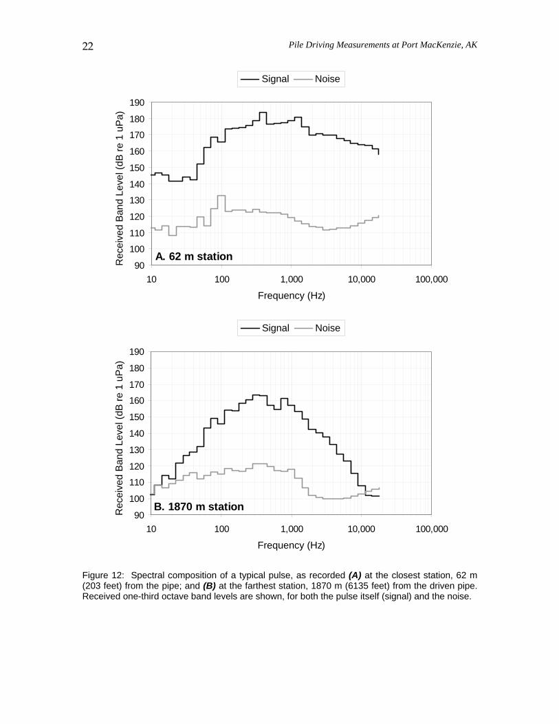
Spectral Analysis (Impact Pile Driving) Figure 12 shows received one-third octave band levels for a typical pulse at two

boat-based stations: the closest (62 m or 203 feet, Fig. 12A) and the farthest (~1870 m or 6135 feet, Fig. 12B). Values for both the signal and noise are shown; noise levels were computed from the period directly preceding each impact pulse, and signal levels were obtained by subtracting noise levels from signal + noise levels (after conversion to pressure squared). Peak SPL for the pile driving pulse was at the one-third octave bands centered at 446 and 354 Hz for the close and far stations, respectively. Pulse energy was spread over a wide range of frequencies, but mostly 100–2000 Hz.

(The remainder of this page was left blank intentionally)


22

90

100

110

120

130

140

150

160

170

180

190

10 100 1,000 10,000 100,000

Frequency (Hz)

Rec

eive

d B

and

Leve

l (dB

re 1

uP

a)

Signal Noise

A. 62 m station

90

100

110

120

130

140

150

160

170

180

190

10 100 1,000 10,000 100,000

Frequency (Hz)

Rec

eive

d B

and

Leve

l (dB

re 1

uP

a)

Signal Noise

B. 1870 m station

Figure 12: Spectral composition of a typical pulse, as recorded (A) at the closest station, 62 m (203 feet) from the pipe; and (B) at the farthest station, 1870 m (6135 feet) from the driven pipe. Received one-third octave band levels are shown, for both the pulse itself (signal) and the noise.


23

DISCUSSION

Vibratory Pile Driving

Received broadband levels during vibratory pile driving reached mean values of 163–164 dB re 1 µPa 56 m (184 feet) from the driven pipe at both hydrophone depths. Levels decreased with distance from the source by 21.8 and 28.9 dB/tenfold change in distance for the deep and shallow hydrophones, respectively. Most of the energy during vibrating activity was in the range 400–2500 Hz. In addition, there were strong tones at 15 Hz and multiples thereof.

Comparison of the data reported here with other vibratory pile driving measurements is hampered by the paucity of similar studies — the five studies listed below were either conducted in much shallower water than the present study, or the piles were not driven directly into the water, but rather on adjacent land.

• Burgess and Blackwell (2005) measured SPLs during vibratory pile driving of an H-pile in the Snohomish River, Washington. They report broadband (4–10,000 Hz) levels of ~160 dB at a distance of 14 m (46 feet), with most of the sound energy in a tone varying between 12 and 18 Hz. Broadband levels had decreased to ~114 dB by 340 m (1115 feet). Water depth was very shallow (~5 m or 16 feet), which leads to poor propagation of low frequencies.

• Nedwell and Edwards (2002) measured SPLs during the use of a PTC 60HD vibro driver during the driving of piles in a river. They report levels of 151 dB re 1 µPa at a distance of 80 m, which is about 13 dB below values expected at that distance in this study. However, water depth during those measurements was extremely shallow, on the order of 0.5 m (1.6 feet), which again makes comparisons difficult.

• Two studies made recordings of vibratory pile driving sounds at Northstar Island, in the Alaskan Beaufort Sea. In both studies sheet piles were driven into a gravel island, about 40 m (131 feet) from the shoreline. Greene and McLennan (manuscript) report received sound pressure levels of the vibratory tone (23–25 Hz) of 115–117 dB re 1 µPa at distances of 300–400 m (984–1312 feet). Shepard et al. (2001) do not give any broadband levels, but from spectra and one-third octave band levels we can infer that the broadband levels (2–20,000 Hz) were close to 120 dB re 1 µPa at a distance of 150 m. These values are 20–30 dB less than the present study, but the fact that the Northstar piles were driven into gravel distant from the water accounts for much of the difference.

• Finally, Burgess and Blackwell (2003) measured SPLs during the use of a vibrating beam to inject a wall of self-hardening slurry into the ground, to prevent toxins from leaching into a river from a contaminated site. They report typical broadband values of 140–150 dB re 1 µPa at a distance of 64 m (210 feet). This is ~15–25 dB below the values obtained in this report, but again the situations are not directly comparable since the vibrating activity was taking place into soil, not the river itself.


24

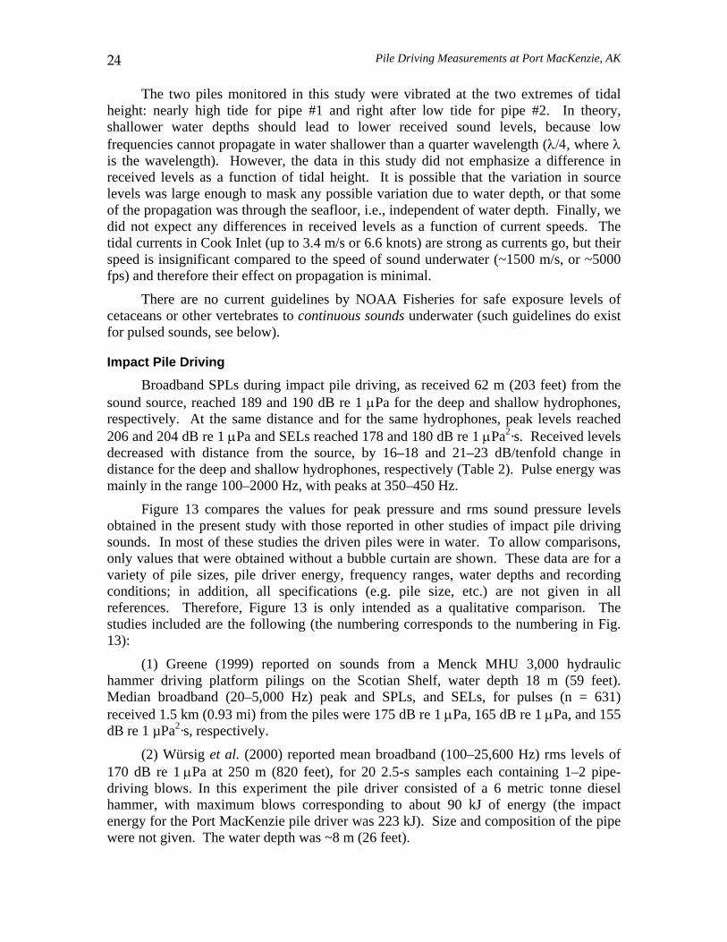
The two piles monitored in this study were vibrated at the two extremes of tidal height: nearly high tide for pipe #1 and right after low tide for pipe #2. In theory, shallower water depths should lead to lower received sound levels, because low frequencies cannot propagate in water shallower than a quarter wavelength (λ/4, where λ is the wavelength). However, the data in this study did not emphasize a difference in received levels as a function of tidal height. It is possible that the variation in source levels was large enough to mask any possible variation due to water depth, or that some of the propagation was through the seafloor, i.e., independent of water depth. Finally, we did not expect any differences in received levels as a function of current speeds. The tidal currents in Cook Inlet (up to 3.4 m/s or 6.6 knots) are strong as currents go, but their speed is insignificant compared to the speed of sound underwater (~1500 m/s, or ~5000 fps) and therefore their effect on propagation is minimal.

There are no current guidelines by NOAA Fisheries for safe exposure levels of cetaceans or other vertebrates to continuous sounds underwater (such guidelines do exist for pulsed sounds, see below).

Impact Pile Driving

Broadband SPLs during impact pile driving, as received 62 m (203 feet) from the sound source, reached 189 and 190 dB re 1 µPa for the deep and shallow hydrophones, respectively. At the same distance and for the same hydrophones, peak levels reached 206 and 204 dB re 1 µPa and SELs reached 178 and 180 dB re 1 µPa2·s. Received levels decreased with distance from the source, by 16–18 and 21–23 dB/tenfold change in distance for the deep and shallow hydrophones, respectively (Table 2). Pulse energy was mainly in the range 100–2000 Hz, with peaks at 350–450 Hz.

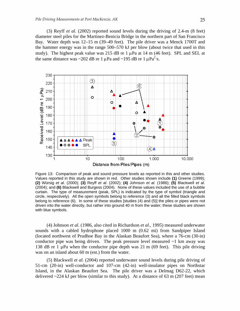
Figure 13 compares the values for peak pressure and rms sound pressure levels obtained in the present study with those reported in other studies of impact pile driving sounds. In most of these studies the driven piles were in water. To allow comparisons, only values that were obtained without a bubble curtain are shown. These data are for a variety of pile sizes, pile driver energy, frequency ranges, water depths and recording conditions; in addition, all specifications (e.g. pile size, etc.) are not given in all references. Therefore, Figure 13 is only intended as a qualitative comparison. The studies included are the following (the numbering corresponds to the numbering in Fig. 13):

(1) Greene (1999) reported on sounds from a Menck MHU 3,000 hydraulic hammer driving platform pilings on the Scotian Shelf, water depth 18 m (59 feet). Median broadband (20–5,000 Hz) peak and SPLs, and SELs, for pulses (n = 631) received 1.5 km (0.93 mi) from the piles were 175 dB re 1 µPa, 165 dB re 1 µPa, and 155 dB re 1 µPa2·s, respectively.

(2) Würsig et al. (2000) reported mean broadband (100–25,600 Hz) rms levels of 170 dB re 1 µPa at 250 m (820 feet), for 20 2.5-s samples each containing 1–2 pipe-driving blows. In this experiment the pile driver consisted of a 6 metric tonne diesel hammer, with maximum blows corresponding to about 90 kJ of energy (the impact energy for the Port MacKenzie pile driver was 223 kJ). Size and composition of the pipe were not given. The water depth was ~8 m (26 feet).


25

(3) Reyff et al. (2002) reported sound levels during the driving of 2.4-m (8 feet) diameter steel piles for the Martinez-Benicia Bridge in the northern part of San Francisco Bay. Water depth was 12–15 m (39–49 feet). The pile driver was a Menck 1700T and the hammer energy was in the range 500–570 kJ per blow (about twice that used in this study). The highest peak value was 215 dB re 1 µPa at 14 m (46 feet). SPL and SEL at the same distance was ~202 dB re 1 µPa and ~195 dB re 1 µPa2·s.

Figure 13: Comparison of peak and sound pressure levels as reported in this and other studies. Values reported in this study are shown in red. Other studies shown include (1) Greene (1999); (2) Würsig et al. (2000); (3) Reyff et al. (2002); (4) Johnson et al. (1986); (5) Blackwell et al. (2004); and (6) Blackwell and Burgess (2004). None of these values included the use of a bubble curtain. The type of measurement (peak, SPL) is indicated by the type of symbol (triangle and circle, respectively). All the open symbols belong to reference (3) and all the filled black symbols belong to reference (6). In some of these studies [studies (4) and (5)] the piles or pipes were not driven into the water directly, but rather into ground 40 m from the water; these studies are shown with blue symbols.

(4) Johnson et al. (1986, also cited in Richardson et al., 1995) measured underwater sounds with a cabled hydrophone placed 1000 m (0.62 mi) from Sandpiper Island (located northwest of Prudhoe Bay in the Alaskan Beaufort Sea), where a 76-cm (30-in) conductor pipe was being driven. The peak pressure level measured ~1 km away was 138 dB re 1 µPa when the conductor pipe depth was 21 m (69 feet). This pile driving was on an island about 60 m (est.) from the water.

(5) Blackwell et al. (2004) reported underwater sound levels during pile driving of 51-cm (20-in) well-conductor and 107-cm (42-in) well-insulator pipes on Northstar Island, in the Alaskan Beaufort Sea. The pile driver was a Delmag D62-22, which delivered ~224 kJ per blow (similar to this study). At a distance of 63 m (207 feet) mean


26

peak and SPLs reached 157 and 151 dB re 1 µPa, respectively; SELs reached 145 dB re 1 µPa2·s. The pipes were driven on land, about 43 m (141 feet) from the water’s edge.

(6) Blackwell and Burgess (2004) reported underwater sound levels during pile driving of 2.4-m (8-foot) steel piles at the reconstruction of the San Francisco-Oakland Bay Bridge. The pile driver was a Menck 1700T with a 180 ton hammer and a maximum net impact energy of 1870 kJ (about six times that used in this study). Water depth around the piles was 8 m (26 feet).

Values reported in the studies by Greene (1999), Reyff et al. (2002), Würsig et al. (2000) and Blackwell and Burgess (2004) are comparable to those in the present study. In all those studies, the piles were in the water. All but the Würsig et al. (2000) study used pile drivers with higher maximum hammer energies than the present study. However, the hammer energy setting may have been set at a lower value [as it was in Reyff et al. (2002)] and we have no information on that aspect for most of the studies. In addition, measurements by Blackwell and Burgess (2004) showed that hammer size per se had a very small effect on sound pressure levels received. In that study, recordings were obtained with a Menck 1700T and a Menck 500T hammer, which have maximum net impact energies of 1870 and 550 kJ, respectively. At a distance of 100 m and for a hydrophone depth of 7 m, the difference between the two hammers in mean received SPL, peak and SEL was 1, 1, and 2 dB, respectively. Substrate composition is likely of greater importance in determining the sound pressure levels produced during pile driving.

The much lower values in the study by Blackwell et al. (2004), comparable to Johnson et al. (1986), are likely due to the fact that the pipes were driven into the gravel island and not directly into the water.

Pulse length tended to increase with distance from the pipe, but with much variation (Fig. 11). This is to be expected, as geometric dispersion spreads the pulse with distance from the source. The Eagle Bay B-Probe (station A5) was located the farthest distance from the driven pipe, and had the longest pulse lengths, 0.41–0.48 s (Table 3). This is about twice the length of the Cairn Point B-Probe (station A4) pulses shown in Fig. 11.

Spectral analyses of the pulses (see Fig. 12) showed that most of the pulse energy was found in the one-third octave bands centered at 100–2000 Hz. Comparable frequency ranges as shown in other studies were 80–500 Hz in Blackwell and Burgess (2004) and 50–350 Hz for Reyff et al. (2002). The pulse spectral distribution was similar at the closest and farthest stations (Fig. 12). For a given set of steel piles the differences in bandwidth of the received levels are most likely related to differences in the size, length and thickness of the piles – this is analogous to bigger bells with thicker walls having lower frequencies than smaller bells with thinner walls.

NOAA Fisheries has specified that cetaceans should not be exposed to pulsed sounds exceeding 180 dB re 1 µPa SPL, i.e., root-mean-square value averaged over the pulse duration (NMFS 2000). According to the logarithmic sound propagation model that was fitted to the data (see Fig. 8), mean SPLs decreased below 180 dB re 1 µPa at distances of 250 m and 195 m (820 feet and 640 feet) for the deep and shallow hydrophones, respectively. To be conservative, we can use the highest values obtained for each hydrophone depth and the corresponding sound propagation formulas to


27

calculate the distance beyond which SPLs would be below 180 dB. The highest received SPLs were obtained at a mean distance of 129 m (423 feet) from the pipe and reached 192 and 190 dB re 1 µPa for the deep and shallow hydrophones, respectively (Fig. 8). Using these data, the distances beyond which SPLs would decrease below 180 dB are 650 m and 330 m (2133 feet and 1083 feet) for the deep and shallow hydrophones, respectively.

Water depth as determined by the tide was about the same for the two pipes driven using impact pile driving. Therefore we did not expect an effect of tidal state on received levels.

Background Levels

The lower range of broadband (10–10,000 Hz) background levels obtained in this study at Port MacKenzie was 115–133 dB re 1 µPa for both hydrophone depths. Note that these levels were not “ambient” levels in the sense that they were obtained close to an industrialized area (Anchorage) and were not devoid of industrial sounds. Rather, they strictly represent the levels while vibratory or impact pile driving were not taking place, but other industrial activities were discernable on the recordings. In addition, some of these background levels were obtained with strong currents while the recording vessel was tied up, resulting in a large contribution of flow noise. Blackwell and Greene (2003) made recordings of background levels in Cook Inlet in 2001, in areas with and without industrial noise. Broadband values ranged from less than 95 dB re 1 µPa at Birchwood in Knik Arm to over 120 dB re 1 µPa for locations off Elmendorf AFB and north of Point Possession during the incoming tide. The values obtained in this study in the absence of vibratory pile driving and without strong currents (115–118 dB re 1 µPa), were comparable to the values obtained in Cook Inlet in 2001. The values obtained in the absence of impact pile driving (125–132 dB re 1 µPa), i.e., while the tide was incoming or outgoing, were somewhat higher than the 2001 measurements.

Acknowledgments

From LGL, I wish to thank Guy Wade for being the boat driver during the recordings, Melissa Cunningham for helping with fieldwork and Michael Williams for his leadership and guidance during the project, as well as his review of this report. Dr. Bill Burgess analyzed the Eagle Bay pulses. Drs. Bill Burgess and Charles Greene (Greeneridge Sciences), as well as Dr. Mardi Hastings (Ohio State University) reviewed drafts of the report and provided many useful comments – I thank them all.

LITERATURE CITED

Angliss, R.P. and K.L. Lodge. (2003). Beluga whale: Cook Inlet stock. In Draft Alaska Marine Mammal Stock Assessments, NMML.

Blackwell, S.B., and C.R. Greene, Jr. (2003). Acoustic measurements in Cook Inlet, Alaska, during August 2001. Greeneridge Rep. 271-2. Rep. from Greeneridge Sciences, Inc., Santa Barbara, CA, for NMFS, Anchorage, AK. 43 p.

Blackwell, S.B., and W.C. Burgess. (2004). Underwater measurements of pile-driving


28

sounds during the San Francisco-Oakland Bay Bridge East Span seismic safety project. Greeneridge Rep. 305-1. Rep. from Greeneridge Sciences, Inc., Santa Barbara, CA, for Illingworth and Rodkin, Inc., Petaluma, CA. 19 p.

Blackwell, S.B., J.W. Lawson and M.T. Williams. (2004). Tolerance by ringed seals (Phoca hispida) to impact pipe-driving and construction sounds at an oil production island. J. Acoust. Soc. Am. 115(5), 2346–2357.

Burgess, W.C., and C.R. Greene, Jr. (1999). Physical acoustics measurements, p. 3–1 to 3–65 In: W.J. Richardson (ed.), Marine mammal and acoustical monitoring of Western Geophysical’s open-water seismic program in the Alaskan Beaufort Sea, 1998. LGL Rep. TA2230-3. Rep. from LGL Ltd., King City, Ont., and Greeneridge Sciences Inc., Santa Barbara, CA, for Western Geophysical, Houston, TX, and Nat. Mar. Fish. Serv., Anchorage, AK, and Silver Spring, MD. 390 p.

Burgess, W.C., and S.B. Blackwell. (2003). Acoustic monitoring of barrier wall installation at the former Rhône-Poulenc site, Tukwila, Washington. Greeneridge Rep. 290-1. Rep. from Greeneridge Sciences, Inc., Santa Barbara, CA, for RCI Environmental, Inc., Sumner, WA. 28 p.

Burgess, W.C., and S.B. Blackwell. (2005). Underwater sounds of vibratory pile driving in the Snohomish River, Everett, Washington. Greeneridge Rep. 322-2. Rep. from Greeneridge Sciences, Inc., Santa Barbara, CA, for URS Corporation, Seattle, WA. 35 p.

Ferrero, R.C., S.E. Moore, and R.C. Hobbs. (2000). Development of beluga, Delphinapterus leucas, capture and satellite tagging protocol in Cook Inlet, Alaska. Mar. Fish. Rev. 62(3):112–123.

Funk, D.W., R.J. Rodrigues and M.T. Williams (eds.). (2005). Baseline studies of beluga whale habitat use in Knik Arm, Upper Cook Inlet, Alaska. Rep. from LGL Alaska Research Associates, Inc., Anchorage, AK, for HDR Alaska, Inc., Anchorage, AK, and Knik Arm Brige and Toll Authority, Anchorage, AK. 65 p. + App.

Greene, C.R., Jr. (1999). Pile-driving and vessel sound measurements during installation of a gas production platform near Sable Island, Nova Scotia, during March and April, 1998. Rep. 205-2. Report by Greeneridge Sciences Inc., Santa Barbara, CA and LGL Ltd., environmental research associates, King City, Ont., for Sable Offshore Energy Project, Halifax, NS. Available from ExxonMobil Canada, PO Box 517, Halifax, NS, B3J 2R7 Canada.

Greene, C.R., Jr, and M.W. McLennan (MS). Sounds and vibrations from vibratory and impact sheet-pile driving at a gravel island in the frozen Beaufort Sea.

Johnson, S.R., C.R. Greene, Jr., R.A. Davis, and W.J. Richardson. (1986). Bowhead whales and underwater noise near the Sandpiper Island drillsite, Alaskan Beaufort Sea, autumn 1985. Rep. from LGL Ltd., King City, Ont., and Greeneridge Sciences Inc., Santa Barbara, CA, for Shell Western E & P Inc., Anchorage, AK. 130 p.


29

Malme, C.I., C.R. Greene, Jr., and R.A. Davis. (1998). Comparison of radiated noise from pile-driving operations with predictions using the RAM model. LGL Rep. TA2224-2. Report by LGL Ltd., environmental research associates, King City, Ont., Engineering and Scientific Services, Hingham, MA, and Greeneridge Sciences Inc., Santa Barbara, CA for Sable Offshore Energy Project, Halifax, NS, Canada. Available from ExxonMobil Canada, PO Box 517, Halifax, NS, B3J 2R7 Canada.

McCauley, R.D., M.-N. Jenner, C. Jenner, K.A. McCabe, and J. Murdoch. (1998). The response of humpback whales (Megaptera novaeangliae) to offshore seismic survey noise: preliminary results of observations about a working seismic vessel and experimental exposures. APPEA (Australian Petroleum Production and Exploration Association) Journal 38, 692–707.

McCauley, R.D., J. Fewtrell, A.J. Duncan, C. Jenner, M.-N. Jenner, J.D. Penrose, R.I.T. Prince, A. Adhitya, J. Murdoch, and K.A. McCabe. (2000). Marine seismic surveys - A study of environmental implications. APPEA J., 40, 692–708.

Morsell, J., J. Houghton, and K. Turco. (1983). Knik Arm Crossing Project Marine Biological Studies. Technical Memorandum No. 15 for the Alaska Department of Transportation and Public Facilities. 51 p. + App.

Nedwell, J, and B. Edwards. (2002). Measurements of underwater noise in the Arun River during piling at County Wharf, Littlehampton. Subacoustech Rep. 513 R 0108. Report by Subacoustech Ltd., Soberton Heath, Hants, for David Wilson Homes Ltd, Horsham, West Sussex, Great Britain. Available at http://www.subacoustech.com.

NMFS. (2000). Taking and importing marine mammals; taking marine mammals incidental to construction and operation of offshore oil and gas facilities in the Beaufort Sea. Fed. Regist. 65(102, 25 May), 34014–34032.

Reyff, J.A., P.P. Donovan and C.R. Greene, Jr. (2002). Underwater sound levels associated with construction of the Benicia-Martinez Bridge. Preliminary Results, Illingworth & Rodkin, Inc., 14 August 2002.

Richardson, W.J., C.R. Greene, Jr., C.I. Malme, and D.H. Thomson. (1995). Marine Mammals and Noise (Academic Press, San Diego, CA), pp. 127–132, 346.

Rugh, D.J., K.E.W. Shelden and B.A. Mahoney. (2000). Distribution of belugas, Delphinapterus leucas, in Cook Inlet, Alaska, during June/July 1993–2000. Mar. Fish. Rev. 62(3), 6–21.

Shepard, G.W., P.A. Krumhansl, M.L. Knack, and C.I. Malme. (2001). ANIMIDA Phase I: ambient and industrial noise measurements near the Northstar and Liberty sites during April 2000. BBN Tech. Memo. 1270; OCS Study MMS 2001–0047. Rep. by BBN Technologies Inc., Cambridge, MA, for U.S. Minerals Manage. Serv., Anchorage, AK.

Würsig, B., C.R. Greene, Jr., and T.A. Jefferson. (2000). Development of an air bubble curtain to reduce underwater noise of percussive piling. Mar. Environ. Res. 49, 79–93.


30

APPENDIX A

Review of “Chapter 4: Underwater Measurements of Pile Driving Sounds

during the Port MacKenzie Dock Modifications”

by

Mardi C. Hastings, P.E., Ph.D.

This report provides a thorough discussion and analysis of measurements of underwater sound generated by vibratory and impact pile driving in the Knik Arm during modifications of the Port MacKenzie dock. Underwater sounds were recorded continuously at three fixed locations using Bioacoustic Probes (B-Probes), and intermittently at different distances from the pile using ITC 1032 hydrophones deployed from a boat. Because sound pressure could vary with water depth, two ITC hydrophones were deployed simultaneously at two different depths for these measurements. From the description and maps provided in the report, the Knik Arm appears to be a narrowing of the Cook Inlet with depth exceeding 40 m near the middle and gradually becoming shallower towards shore on both sides. There appears to be no major obstructions. Although the report stated that currents could be rather strong in this area, they are much slower than the speed of sound so they would have had little, if any, effect on the measurements as indicated by the author. The B-Probe has a self-contained hydrophone and digital recorder with a sampling rate of 6554 Hz. Signals from the ITC hydrophones were recorded with a Sony DAT recorder at a sampling rate of 24,000 Hz. Thus frequency content of the data recorded by the B-Probes was limited to about 3250 Hz, while data recorded with the Sony DAT was limited to about 12,000 Hz. These bandwidths are appropriate for pile driving sounds, which usually contain most energy below 2000 Hz. The B-Probes were limited to a peak pressure of about 190 dB re 1 µPa; however, they were placed at locations far enough away from the pile that peak pressure would not have been expected to exceed this level. The sensitivity of the ITC 1032 hydrophones was reduced with a shunt capacitor, presumably to prevent clipping of the expected impact signals and possible damage to the transducers. Sound generated from a single impact of a large diameter steel pile is a pulse that has extremely large positive and negative pressure excursions over a few milliseconds. As is done in this report, it is generally characterized by quantities that have been associated with biological effects on humans and terrestrial mammals. These include peak pressure (whether positive or negative), sound pressure level (SPL) based on a root-mean-square (rms) average over the time duration of the pulse, sound exposure level (SEL), and spectral density (a measure of estimated sound energy as a function of frequency) or received sound level over a defined frequency band (such as one-third octave bands). The pulse duration must be defined to calculate SPL and SEL, and it is accepted practice to define it as the time interval between the arrival of 5% and 95% of the total sound energy. However, the accumulation of sound energy over time cannot be determined


31

exactly unless both the instantaneous sound pressure and particle velocity associated with passage of the pulse are known. The product of the instantaneous sound pressure and particle velocity is the acoustic intensity, which is the power flow per unit area. So the true received sound energy per unit area is the time integral of the intensity; consequently, accumulation of sound energy is roughly estimated by integrating the square of the instantaneous sound pressure over time as was done in this study. The pulse duration is then defined as the time interval between accumulation of 5% and 95% of the total “estimated” sound energy. Because SEL is the square of the instantaneous pressure integrated over the pulse duration and not calculated from the true acoustic intensity, it is only “roughly related to the energy in the pulse” as stated in the report. The SPL calculated over a time duration defined in this way is sometimes called an “rms90%” average, rather than just rms, because it is associated with 90% of the estimated sound energy in the pulse. Very few measurements have been made of continuous, non-impulsive sounds from vibratory pile driving. Determining the rms of representative 8.5-second segments of the recorded sound pressure is a reasonable approach. For the lowest frequency of 4 Hz, an 8.5-second segment would contain over 30 cycles and usually signals are assumed to be continuous if they have over 10 cycles. This report presents the mean and standard deviation of SPL’s at different distances from the pile (pipe) during vibratory driving, and the mean and standard deviation of peak pressures, SPL’s, and SEL’s at different distances from the pile during impact driving. These data are shown to correlate well with a simple sound propagation model based on logarithmic spreading. This type of empirical model is usually valid in regions where the underwater environment is relatively simple. As indicated in the report, it is valid only within the range of distances that data were recorded and should not be used to extrapolate received levels at distances beyond the locations of measured data. It is also important to note that the received levels reported for impact driving are the average value for a single pulse and are not representative of the cumulative sound energy that would be received from multiple sound pulses. The sound levels recorded in the Knik Arm for vibratory and impact driving of steel pipes compare well with levels reported for similar types of pile driving operations in other locations. These comparisons are summarized in the Discussion section of the report. Data from several recent impact pile driving studies are plotted together in Figure 4.13 and clearly show consistency in received sound levels for driving of large diameter steel piles (pipes) in relatively simple underwater environments. The differences in frequency bandwidths of impact pile driving sounds in these studies that were noted in the report, are primarily caused by differences in the length, diameter and wall thickness of the pile or pipe, the properties of the ocean bottom, and the coupling between the pile and hammer. Detailed Comments/Suggestions Executive Summary, 1st paragraph: Need to state that these piles are 36”-diameter steel piles (or pipes). The sound levels reported are about the same for other large steel piles. Executive Summary, 2nd paragraph: State that the SPL is rms; also it seems out of place to give precision to a tenth of a dB for the decrease per tenfold change in distance when this precision is not used with any other levels reported on this page. Suggest


32

summarizing the rms SPL, decrease w/distance and frequency information for vibratory and impact pile driving in a Table as it would be much clearer. Executive Summary, 3rd paragraph: Suggest replacing “Pulse energy” with “Sound energy in the pulse” at the beginning of the last sentence. Introduction, 2nd line: Suggest changing end of 1st sentence to read “…maintain a crossing that will span the….” to replace the “.a crossing across the…” Below Table 4.1, 3rd line under Signal Analysis sub-heading: Believe the data bandwidth should be 4-12,000 Hz if sampling rate was 24 kHz. Also in same paragraph – need registered trademark symbol at end of “MATLAB” and suggest stating the Version of MATLAB that you used because different versions can give different computational results. 1st paragraph under Broadband Analysis (under Signal Analysis): Need to state more clearly that the peak pressure can be positive or negative – maybe say “absolute value of the sound pressure” rather than “absolute sound pressure.” Suggest using “total estimated sound energy in the pulse” in place of “total pulse energy” because “pulse energy” is, more accurately, the sound energy and since the accumulation of pressure-squared defines the pulse, it is only an estimate of the sound energy. 3rd paragraph under Broadband Analysis (under Signal Analysis): In 6th line suggest replacing “in order” with “so” Figure 4.4: The vertical axes labels should be just “Pressure” or “Sound Pressure.” Best to use Sound Pressure Level only when referring to SPL in dB. Also suggest removing “level” in the figure caption. 1st paragraph after Figure 4.4, last sentence: Suggest changing “received level vs. range” to “received level vs. distance” since the axes of the plots are labeled “distance” and the word “range” is used again in this sentence with reference to “levels received at several distances.” 2nd paragraph after Figure 4.4: Suggest rewording this sentence to indicate that the data were “fit to” or “correlated with” a logarithmic spreading loss model using the least squares method, rather than the “model was fitted.” 3rd paragraph after Figure 4.4: Suggest replacing “range to” in the first line with “distance from” because later in this paragraph and in the Introduction and Methods sections it states that received levels were measured at a “range of distances” or at various distances from the source. Results section, 4th paragraph: Suggest rewording first sentence to indicate that the data were fitted to a model rather than vice versa – “Received sound pressure level data out to a distance of 1300 m (4265 feet) were fit to the simple logarithmic sound propagation model [Eq. (1)].” 1st paragraph after Table 4.2: Since Figure 4.4 has plots of sound pressure rather than SPL’s, suggest removing the word “level” from the 1st sentence, and replacing the last sentence with the following – “Note the wide temporal variation in sound pressure, independent of the distance to the pipe. Results section: The point needs to be made that mean SPL’s, SEL’s, and Peak received levels are average values for a single hammer impact, not multiple ones as would occur during pile driving operations.


33

Discussion section, 2nd paragraph before “Impact Pile Driving” sub-heading: Suggest rewording end of 2nd sentence to read – “…because low frequencies cannot propagate in water shallower than a quarter wavelength (λ/4, where λ is the wavelength). Discussion section, “Impact Pile Driving” subsection: In this section it is very important to indicate which piles in other studies were made of steel and how large they were. I believe that the piles in studies (1), (3), and (6) were large-diameter steel piles and they were driven in relatively uncomplicated underwater areas, so you would expect the received levels to be similar and follow a logarithmic spreading model. Likewise, given that they are all steel piles, the differences in bandwidth of the received levels as noted in this subsection is most likely related to differences in the size, length and wall thickness of the pile (analogous to bigger bells with thicker walls having lower frequencies than smaller bells with thinner walls). ------------------------------------------------------------------------------------------------------------

About the Reviewer: Dr. Mardi Hastings received a Ph.D. in acoustics from the School of Mechanical

Engineering at the Georgia Institute of Technology. She worked 6 years in industry and 14 years in academia before joining the Office of Naval Research in 2003 as a Program Manager for the Marine Mammal Program and Bioeffects of Non-Lethal Weapons Program. She is an active member of the Acoustical Society of America, the Noise Control and Acoustics Division of the American Society of Mechanical Engineers, and serves as Co-Chair of Team 7 (Noise and Animals) for the International Commission on the Biological Effects of Noise.

Dr. Hastings in the author or co-author of over 50 refereed journal articles and proceedings papers, and more than 100 conference papers, seminars, and workshops. She was a member of the National Academy of Sciences Study Committee on Potential Impacts of Ambient Noise on Marine Mammals, 2001–02 (Final Report, Ocean Noise and Marine Mammals, National Academies Press, Washington, DC, 2003). Currently she is a member of the NOAA/NMFS Expert Panel to Develop Acoustic Safety Guidelines for Fish. She has been a consultant in many areas of acoustics for over 20 years. Projects within the last five years include the Effect of Altitude on Attenuation Constant and Absorption Coefficient of Fiberglass, Owens Corning Science and Technology Center, Granville, OH; Analysis of Acoustic Impact during Pile Driving Operations in San Francisco Bay, Caltrans, Sacramento, CA; Analysis of Gun Blast and Sonic Boom Noise over Open Water and Its Potential Effect on Marine Animals, Covington & Burling, Washington, DC; and Effects of Sound on Fish, Caltrans (subcontract through Jones&Stokes), Sacramento, CA.

Documents

Underwater Measurements of Pile-driving Sounds … Measurements of Pile Driving Sounds during the Port MacKenzie Dock Modifications, 13–16 August 20041 By Susanna B. …