Unemployment and Environmental Regulation in General ... · Resources for the Future Hafstead and Williams 1 Unemployment and Environmental Regulation in General Equilibrium Marc

1616 P St. NW Washington, DC 20036 202-328-5000 www.rff.org

May 2016 RFF DP 15-11

Unemployment and Environmental Regulation in General Equilibrium

Marc A . C . Ha fs tead and Rober ton C . Wi l l i ams I I I

Considering a US Carbon Tax: Economic Analysis and

Dialogue on Carbon Pricing Options www.rff.org/carbontax

DIS

CU

SSIO

N P

AP

ER

© 2016 Resources for the Future. All rights reserved. No portion of this paper may be reproduced without permission of the authors.

Discussion papers are research materials circulated by their authors for purposes of information and discussion. They have not necessarily undergone formal peer review.


Marc A.C. Hafstead and Roberton C. Williams III

Abstract

This paper analyzes the effects of environmental policy on employment (and unemployment) using a new general-equilibrium two-sector search model. We find that imposing a pollution tax causes substantial reductions in employment in the regulated (polluting) industry, but this is offset by increased employment in the unregulated (nonpolluting) sector. Thus the policy causes a substantial shift in employment between industries, but the net effect on overall employment (and unemployment) is small, even in the short run. An environmental performance standard causes a substantially smaller sectoral shift in employment than the emissions tax, with roughly similar net effects. The effects on the unregulated industry suggest that empirical studies of environmental regulation that focus only on regulated firms can be misleading (and those that use nonregulated firms as controls for regulated firms will be even more misleading). The paper’s results also suggest that overall effects on employment are not a major issue for environmental policy, and that policymakers who want to minimize sectoral shifts in employment might prefer performance standards over environmental taxes.

Key Words: unemployment, environmental regulation, emissions pricing, climate,

environmental tax, intensity standard

JEL Classification Numbers: Q58, Q52, H23, E23, J64

Contents

1. Introduction ......................................................................................................................... 1

2. A Two-Sector Model ........................................................................................................... 3

2.1 Matching Process .......................................................................................................... 4

2.2. Households ................................................................................................................... 5

2.3 Firms ............................................................................................................................. 7

2.4 Wage Bargaining .......................................................................................................... 8

2.5 Government................................................................................................................... 9

2.6 Emissions Taxes and Performance Standards ............................................................. 10

2.7 Consumption Good and Market Clearing ................................................................... 10

3. Calibration ......................................................................................................................... 11

3.1 Household ................................................................................................................... 11

3.2 Firms ........................................................................................................................... 12

3.3 Matching ..................................................................................................................... 13

4. Emissions Tax .................................................................................................................... 13

4.1 Aggregate Unemployment and Employment by Sector ............................................. 15

4.2 Labor Market Outcomes ............................................................................................. 19

4.3 Welfare ........................................................................................................................ 20

4.4 Stringency ................................................................................................................... 21

5. Model Extensions .............................................................................................................. 23

5.1 Wages .......................................................................................................................... 23

5.2 Sensitivity Analysis .................................................................................................... 27

6. Conclusions ........................................................................................................................ 30

References .............................................................................................................................. 33

Resources for the Future Hafstead and Williams

1


Marc A.C. Hafsteada and Roberton C. Williams IIIa, b, c

1. Introduction

Effects on employment have played a central role in the political debate over

environmental regulations, especially during the recent economic downturn, with opponents

deriding regulations as “job killers” and proponents touting “green jobs.” This focus is

understandable, given the large potential welfare effects of involuntary unemployment.

However, economic studies of the effects of environmental regulation do not adequately answer

the question of how regulation affects unemployment.

A substantial number of empirical studies have looked at how regulations affect

employment.1 But while such studies provide valuable information on employment changes in

regulated industries, they do not measure the effects on unregulated industries, so to the extent

that regulation affects employment in those other industries, such studies cannot measure the

overall effect. A more serious problem is that these studies often employ a difference-in-

differences approach, using firms in unregulated industries (or firms in regulated industries, but

in areas that are unregulated or subject to less stringent regulation) as controls. To the extent that

regulation affects employment at those firms, such studies will not only miss the effects on

unregulated firms, but also yield biased estimates of the effects on regulated firms.

Addressing those issues requires a general-equilibrium analysis. But existing general-

equilibrium models used to analyze environmental regulation almost always assume full

employment. And the few models in this area that do allow for unemployment typically focus on

types of unemployment that are largely unimportant in the United States (e.g., unemployment

caused by strong unions that negotiate wages well above free-market levels).2

a Resources for the Future

b University of Maryland

c National Bureau of Economic Research We thank RFF’s New Frontiers Fund and Center for Energy and Climate Economics, Bo Cutter, Paul Balser, and the Linden Foundation for financial support for this work, and seminar participants at the AERE Summer Meetings, the University of Michigan, the National Center for Environmental Economics, Resources for the Future, and the World Congress of Environmental and Resource Economists for helpful comments. 1 For examples, see Berman and Bui (2001), Curtis (2012), Greenstone (2002), and Morgenstern et al. (2002) 2 See, for example, Bovenberg and van der Ploeg (1996).


2

This paper develops a new model to study how environmental regulation affects

employment and unemployment. It incorporates a search model with frictions as in Mortensen

and Pissarides (1994), together with a simple two-sector general-equilibrium model of

environmental policy, roughly calibrated to correspond to the effects of imposing a carbon policy

in the United States. In this model, unemployed workers must search and match with job

openings in each period; the interaction of carbon policy with this matching process plays a key

role in determining the economy-wide employment impacts of the regulation.

This paper makes three substantial contributions. First, we show that while imposing a

pollution tax leads to substantial reductions in employment in the polluting sector of the

economy, those losses are offset by an employment increase of similar magnitude in the

nonpolluting sector, driven both by consumer substitution from polluting to nonpolluting goods

and by decreased competition for workers from the polluting sector, which makes it easier for the

nonpolluting sector to hire. Consequently, while there is a substantial shift in employment

between industries, the net effect on unemployment is small, even in the short run. Empirical

studies that look only at regulated firms would greatly overstate that net effect (though they can

measure the job loss in the regulated sector).3 Difference-in-differences studies that use

unregulated firms as a control group would be even further off, not only missing job gains in

unregulated firms, but also seriously overstating job losses in regulated firms. Our results suggest

that those studies could overstate effects on regulated firms by a factor of almost two and

overstate the overall net effects by far more. This emphasizes the importance of considering

general-equilibrium effects.

Second, we show that the magnitude of the employment shift (both the job losses in the

polluting sector and gains in the nonpolluting sector) is much smaller under a performance

standard (a constraint on pollution emissions per unit of output) than under a pollution tax. A

performance standard is equivalent to a tax on emissions and subsidy on output in the dirty

industry (see, for example, Holland et al. 2009; Fullerton and Metcalf 2001). As a result, the

price increase for polluting goods is much smaller under a performance standard than under an

equivalent emissions tax, and thus the substitution in consumption and corresponding shift in

3 This practice—interpreting estimated effects on the regulated sector as representing the overall effect on

employment—is relatively common. For example, several recent EPA regulatory impact analyses estimate effects on overall employment based on coefficients from Morgenstern et al. (2002) for the effects on regulated industries. Smith et al. (2013) provides an extensive discussion of how EPA has estimated employment effects in regulatory impact analyses.


3

employment is correspondingly smaller. This suggests that, to the extent that policymakers want

to minimize sectoral shifts in employment, performance standards (and related intensity-standard

policies) may be attractive.

Third, the paper develops and demonstrates a tractable framework for bringing

unemployment into computable general equilibrium (CGE) models of environmental regulation.4

This general framework could be useful for studying a wide range of other questions involving

unemployment and environmental regulations, such as questions about the optimal timing of

regulations (e.g., should a major new environmental regulation be implemented during recession,

or would it be better to wait until after the economy has rebounded?), about the design of

regulations (e.g., how is the choice of price-based versus quantity-based regulations affected by

unemployment concerns?), or about the distributional implications of changes in employment

patterns resulting from regulation. And it could readily be adapted to look at employment effects

of other types of policies, such as trade policy, where employment effects play an important

political role.

The rest of the paper is organized as follows. Section 2 presents the structure of the

model. Section 3 explains the calibration of the model, and Section 4 discusses the policy

simulations and results. Section 5 considers extensions of the baseline model, and the final

section offers conclusions.

2. A Two-Sector Model

We begin by introducing a relatively simple two-sector model that will enable us to

analyze the key channels through which environmental policies affect employment in both the

regulated and unregulated sectors. The key element is the inclusion of a search friction as in

Pissarides (1985) and Mortensen and Pissarides (1994). The model is a two-sector extension of

4 Balistreri (2002) provides an alternative approach for integrating unemployment into a CGE model. That paper uses a reduced-form representation, rather than explicitly modeling search as we do. Our approach has a number of advantages, including the ability to look at temporary effects on unemployment resulting from sectoral shifts in demand. Shimer (2013) also looks at employment, with a focus on sectoral shifts caused by environmental policy, but again does not explicitly model search (instead, workers must spend an exogenous amount of time unemployed any time they switch industries) and focuses on a different question (whether labor transition costs should affect the optimal emissions tax). Aubert and Chiroleu-Assouline (2015) explicitly model employment search in a model of environmental taxation but focus only on the long-run steady state, rather than looking at transitions.


4

the Shimer (2010) search model with variable hours.5 The two sectors are the clean sector, c, and

the dirty sector, d.

Hiring is subject to a matching process between recruiters and unemployed workers.

There are no on-the-job searches and no job-to-job transitions: only unemployed workers can

search for jobs. Unemployed workers can search for a job in both sectors. An exogenous and

constant fraction of job matches dissolves each period. All workers are members of a

representative household that provides perfect insurance to its members. This representative

household owns the firms.

2.1 Matching Process

Without loss of generality, we normalize the measure of workers to one. Let denote

the measure of workers in sector . Aggregate employment is given by ; the

unemployment rate (and the measure of unemployed workers) is given by . Unemployed workers search indiscriminately across sectors. Let vj denote the number of recruiters in each

sector. One recruiter, working hj hours, can hire H j ( ) unemployed workers per hour. Labor

market tightness, , is the ratio of aggregate recruiting effort to the number of unemployed

workers, (vjhj )j / (1 n ). Recruiting productivity is therefore endogenous and is a function

of total recruiting activity and the number of unemployed workers. To define recruiting

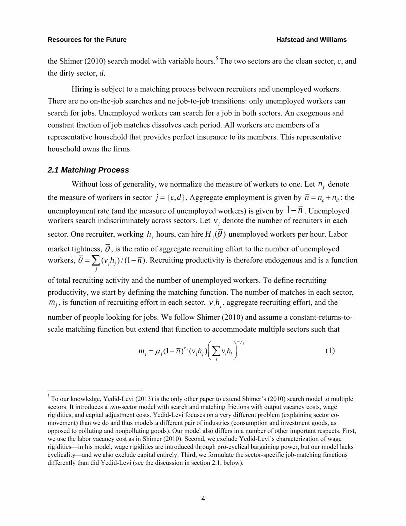
productivity, we start by defining the matching function. The number of matches in each sector, , is function of recruiting effort in each sector, vjhj , aggregate recruiting effort, and the

number of people looking for jobs. We follow Shimer (2010) and assume a constant-returns-to-

scale matching function but extend that function to accommodate multiple sectors such that

mj j (1 n ) j (vjhj ) vii hi

j

(1)

5 To our knowledge, Yedid-Levi (2013) is the only other paper to extend Shimer’s (2010) search model to multiple

sectors. It introduces a two-sector model with search and matching frictions with output vacancy costs, wage rigidities, and capital adjustment costs. Yedid-Levi focuses on a very different problem (explaining sector co-movement) than we do and thus models a different pair of industries (consumption and investment goods, as opposed to polluting and nonpolluting goods). Our model also differs in a number of other important respects. First, we use the labor vacancy cost as in Shimer (2010). Second, we exclude Yedid-Levi’s characterization of wage rigidities—in his model, wage rigidities are introduced through pro-cyclical bargaining power, but our model lacks cyclicality—and we also exclude capital entirely. Third, we formulate the sector-specific job-matching functions differently than did Yedid-Levi (see the discussion in section 2.1, below).

nj

j {c,d} n nc nd

1 n

mj


5

where and are the matching efficiency and matching elasticity parameters for each sector.6

Matches in a given sector are increasing in the number of workers searching for jobs and the

sector’s own recruiting effort. Matches in one sector are decreasing in the recruiting effort of the

other sector as more competition for workers reduces the probability of a match. This represents

an important departure from Yedid-Levi (2013), which assumes that matches in one sector are

independent of recruiting effort in the other sector. That assumption seems unrealistic, given that

both sectors are hiring from the same pool of workers.

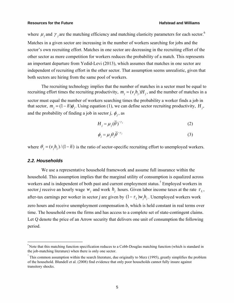
The recruiting technology implies that the number of matches in a sector must be equal to recruiting effort times the recruiting productivity, mj (vjhj )H j , and the number of matches in a

sector must equal the number of workers searching times the probability a worker finds a job in that sector, mj (1 n ) j . Using equation (1), we can define sector recruiting productivity, H j ,

and the probability of finding a job in sector j, j , as

H j j ( ) j (2)

j j j j (3)

where is the ratio of sector-specific recruiting effort to unemployed workers.

2.2. Households

We use a representative household framework and assume full insurance within the

household. This assumption implies that the marginal utility of consumption is equalized across

workers and is independent of both past and current employment status.7 Employed workers in sector j receive an hourly wage and work hours. Given labor income taxes at the rate ,

after-tax earnings per worker in sector j are given by . Unemployed workers work

zero hours and receive unemployment compensation b, which is held constant in real terms over

time. The household owns the firms and has access to a complete set of state-contingent claims.

Let Q denote the price of an Arrow security that delivers one unit of consumption the following

period.

6 Note that this matching function specification reduces to a Cobb-Douglas matching function (which is standard in the job-matching literature) when there is only one sector. 7 This common assumption within the search literature, due originally to Merz (1995), greatly simplifies the problem

of the household. Blundell et al. (2008) find evidence that only poor households cannot fully insure against transitory shocks.

j j

j (vjhj ) / (1 n )

wj hj L

(1 L )wjhj


6

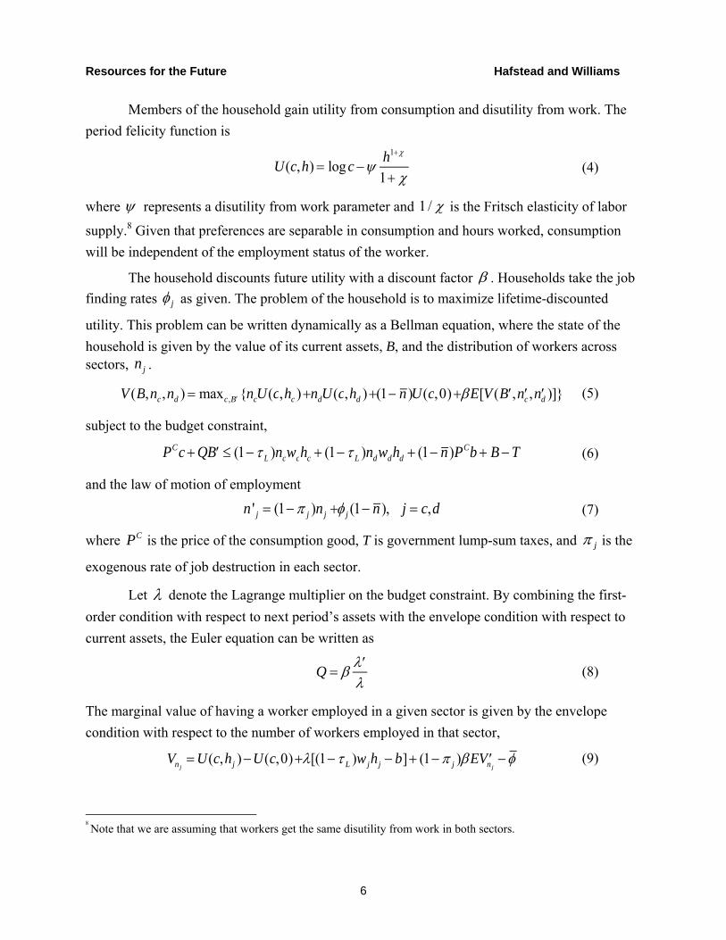
Members of the household gain utility from consumption and disutility from work. The

period felicity function is

(4)

where represents a disutility from work parameter and is the Fritsch elasticity of labor

supply.8 Given that preferences are separable in consumption and hours worked, consumption

will be independent of the employment status of the worker.

The household discounts future utility with a discount factor . Households take the job

finding rates as given. The problem of the household is to maximize lifetime-discounted

utility. This problem can be written dynamically as a Bellman equation, where the state of the

household is given by the value of its current assets, B, and the distribution of workers across sectors, .

(5)

subject to the budget constraint,

(6)

and the law of motion of employment

(7)

where is the price of the consumption good, T is government lump-sum taxes, and is the

exogenous rate of job destruction in each sector.

Let denote the Lagrange multiplier on the budget constraint. By combining the first-

order condition with respect to next period’s assets with the envelope condition with respect to

current assets, the Euler equation can be written as

(8)

The marginal value of having a worker employed in a given sector is given by the envelope

condition with respect to the number of workers employed in that sector,

(9)

8 Note that we are assuming that workers get the same disutility from work in both sectors.

U(c,h) logc h1

1

1/

j

n j

V (B,nc ,nd ) maxc, B {ncU(c,hc )ndU(c,hd )(1 n )U(c,0)E[V ( B , nc , nd )]}

PCc Q B (1 L )ncwchc (1 L )ndwdhd (1 n )PCb B T

n ' j (1 j )nj j (1 n ), j c,d

PC j

Q

VnjU(c,hj )U(c,0)[(1 L )wjhj b] (1 j )E Vnj


7

where . The marginal value consists of utility and compensation

differentials between employed workers in sector j and unemployed workers. The value also

includes the continuation value of being employed in the same job the following period. The

term represents the opportunity cost of being employed (i.e., being unable to look for other

jobs).

2.3 Firms

Firms in each sector produce a sector-specific good using only a labor input, ,

where denotes the number of workers using a production technology that produces units of

output per hour worked. Given a measure of total workers in the beginning of the period, the

firm must decide to allocate workers to production, l j , or recruitment, vj , such that l j vj nj .9

Pollution emissions from production are given by

ej (1 j ) jey j (10)

where unconstrained emissions are a fixed multiple je of net output, yj , and j is the fraction of

unconstrained emissions that are abated. Net output is equal to gross output minus abatement costs, yj yj z j . The cost of abatement is modeled as a per (gross) unit of output cost z such

that

zj z ( j )yj . (11)

The domain of the abatement function z is [0,1]. We assume that z (0) 0, lim1

z ( ) ,

z (0) 0 and z (v) 0 . Firms must pay an emissions tax e for all emissions that are not

abated.10

Firms are owned by households and discount future-period profits with the discount

factor Q from the household problem. Following Shimer (2010), we define the recruiter ratio vj vj / nj . Net output can be written as a function of total workers, the recruiter ratio, and

abatement, yj Ajhjnj (1 vj )(1 z ( j )). Firms take the endogenous recruiting productivity, ,

9 Workers receive the same wage and work the same hours regardless of position. Therefore, workers are indifferent

between job types. 10 If the emissions tax is zero (or if firms have no emissions, as is the case in the clean sector), firms will optimally set abatement to be zero.

cE VncbE Vnd

yj Ajhjl j

l j Aj

nj

H j


8

as given when making recruiter decisions. The dynamic problem of the firm is to choose the

recruiter ratio and abatement to maximize the value of the firm. The Bellman equation is

(11)

subject to

nj (1 j )nj H jvjhjnj (12)

where pjn ( j ) denotes the net price received by sector j for its output and denotes the payroll

tax. The net price of output is equal to the price of the good minus the emissions tax payments, pj

n ( j ) pj e j

e(1 j ). The first-order condition with respect to the recruiter ratio sets the

number of recruiters such that the marginal cost of switching an additional worker from

production to recruitment equals the expected value of recruitment:

(13)

where is the value (to the firm) of an additional worker in the following period. The value of

an additional worker can be derived from the envelope condition with respect to the number of

workers and substituting out equation (14):

(14)

This marginal value of a worker is equal to the marginal revenue minus compensation plus the

expected continuation value times the probability that the match does not exogenously dissolve

at the end of the period. The first-order condition with respect to abatement will equate the

marginal cost of abatement to the marginal benefit of abatement (i.e., lower emissions tax

payments) such that

pjn ( j ) z ( j )

ee(1 z ( j )). (15)

2.4 Wage Bargaining

In each period, the firm and its workers enter a bargaining process to determine hours and the hourly wage. Following Shimer (2010), we assume a Nash bargaining process.11 Let

11 The derivation of the wage and hours equations follows exactly from section 2.4.2 in Shimer (2010). Adding a second sector does not significantly change the derivation, and therefore we omit the derivation here for brevity.

P

Jn j


9

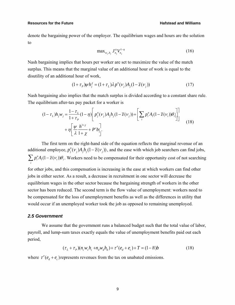
denote the bargaining power of the employer. The equilibrium wages and hours are the solution

to

(16)

Nash bargaining implies that hours per worker are set to maximize the value of the match

surplus. This means that the marginal value of an additional hour of work is equal to the

disutility of an additional hour of work,

(1 P ) hj (1 L ) pn ( j )Aj (1 z ( j )) (17)

Nash bargaining also implies that the match surplus is divided according to a constant share rule.

The equilibrium after-tax pay packet for a worker is

(1 L )hjwj 1 L

1 P

(1) pjn ( j )Ajhj (1 z ( j )) pi

n

i Ai (1 z ( i ))i

h1

1 Pcb

.

(18)

The first term on the right-hand side of the equation reflects the marginal revenue of an additional employee, pj

n ( j )Ajhj (1 z ( j )) , and the ease with which job searchers can find jobs,

pin

i Ai (1 z ( i ))i . Workers need to be compensated for their opportunity cost of not searching

for other jobs, and this compensation is increasing in the ease at which workers can find other

jobs in either sector. As a result, a decrease in recruitment in one sector will decrease the

equilibrium wages in the other sector because the bargaining strength of workers in the other

sector has been reduced. The second term is the flow value of unemployment: workers need to

be compensated for the loss of unemployment benefits as well as the differences in utility that

would occur if an unemployed worker took the job as opposed to remaining unemployed.

2.5 Government

We assume that the government runs a balanced budget such that the total value of labor,

payroll, and lump-sum taxes exactly equals the value of unemployment benefits paid out each

period,

( L P )(ncwchc ndwdhd ) e(ed ec )T (1 n)b (18)

where e(ed ec )represents revenues from the tax on unabated emissions.

maxwj ,hjJn j

Vn j

1


10

2.6 Emissions Taxes and Performance Standards

For simplicity, we assume that the clean sector has zero emissions and therefore c 0

regardless of policy. When e equals zero (the business-as-usual case), the dirty sector has zero incentive to reduce its emissions and therefore abatement is zero (d 0). When e is positive,

the dirty sector will reduce emissions until the marginal cost of abatement equals the marginal

benefit of reducing the emissions tax (as seen in equation (16)). As we always assume a balanced

budget, the introduction of an emissions tax (or an increase in the emissions tax) will require

decreases in lump-sum taxes, labor taxes, payroll taxes, or some combination of all three taxes.

Performance standards are policies that restrict the dirty sector’s emissions per unit of

output. Rewriting equation (10), emissions per unit output are simply equal to the fixed emissions coefficient and abatement, ej / yj (1 j ) j

e . A performance standard is modeled as a

restriction on emissions per unit of output such that they must be less than or equal to some maximum, ej / yj ej . This constraint is isomorphic to a minimum constraint on abatement and

can be implemented directly using a constrained maximization problem; equation (16) is

replaced by

pj Aj (1 vj )hjnz z ( j ) je j

e (19)

where je is the shadow value of the constraint.

2.7 Consumption Good and Market Clearing

The consumption good is created by aggregating the output of the two sectors according

to a constant elasticity of substitution (CES) aggregation function. The price of the consumption

good is

Pc ( c ) c

1 c j c

j pj

1 c

1

1 c

(20)

where j is the CES share parameter for good j, is the CES scaling parameter, and is the

elasticity of substitution between the clean and dirty sectors in consumption. The amount of

consumption demanded by each sector can then be written as

cj ( c j ) c p j

Pc

c

C (21)

Markets clear in each sector when net output is equal to consumption demand,

. (22)

c c

yj cj


11

3. Calibration

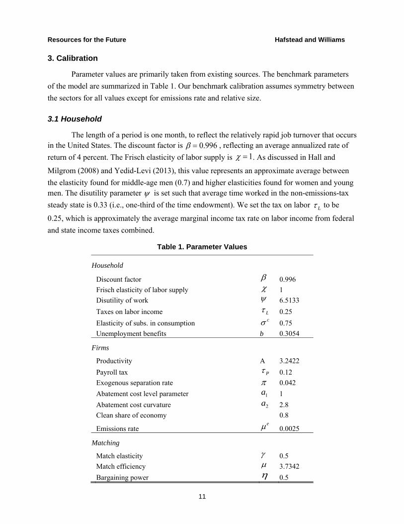
Parameter values are primarily taken from existing sources. The benchmark parameters

of the model are summarized in Table 1. Our benchmark calibration assumes symmetry between

the sectors for all values except for emissions rate and relative size.

3.1 Household

The length of a period is one month, to reflect the relatively rapid job turnover that occurs in the United States. The discount factor is , reflecting an average annualized rate of

return of 4 percent. The Frisch elasticity of labor supply is . As discussed in Hall and

Milgrom (2008) and Yedid-Levi (2013), this value represents an approximate average between

the elasticity found for middle-age men (0.7) and higher elasticities found for women and young men. The disutility parameter is set such that average time worked in the non-emissions-tax

steady state is 0.33 (i.e., one-third of the time endowment). We set the tax on labor to be

0.25, which is approximately the average marginal income tax rate on labor income from federal

and state income taxes combined.

Table 1. Parameter Values

Household

Discount factor 0.996

Frisch elasticity of labor supply 1

Disutility of work 6.5133

Taxes on labor income 0.25

Elasticity of subs. in consumption 0.75

Unemployment benefits b 0.3054

Firms

Productivity A 3.2422

Payroll tax 0.12

Exogenous separation rate 0.042

Abatement cost level parameter a1 1

Abatement cost curvature a2 2.8

Clean share of economy 0.8

Emissions rate 0.0025

Matching

Match elasticity 0.5

Match efficiency 3.7342

Bargaining power 0.5

0.996 1

L

L

c

P

e


12

We do not calibrate the value of unemployment benefits b to an empirical measure of the

replacement rate. Rather, we find the value of b to satisfy the wage bargaining equation given the

calibration of the other parameters. The implied value of b implies a replacement rate of

approximately 42 percent (unemployment benefits as a percentage of after-tax earnings). This

value is much larger than the 25 percent value used by Hall and Milgrom (2008), but it closely

matches values used in other studies (for example, Amaral and Tasci 2013).

We assume an unemployment rate of 7 percent in the non-emissions-tax equilibrium. In

2012, personal consumption expenditures in the United States were approximately $11.1

trillion12; we set consumption equal to $11.1 trillion and then scale by $11.1 trillion such that the

unit of consumption in our non-emissions-tax steady state is one. Through our CES aggregation

function, we assume that the clean and dirty outputs are imperfect substitutes in consumption.

We set the elasticity of substitution in our base case to be a conservative 0.75.13 We then vary

that value in the sensitivity analysis.

3.2 Firms

We begin by assuming that the clean sector is 80 percent of both consumption and labor

(this implies symmetric production productivity parameters).14 Given this assumption, we can

then derive total output and labor employed by sector. Using the steady state value of the

recruiter share (derived in the following section), we calibrate productivity in each sector such that .

According to the Job Openings and Labor Turnover Survey (JOLTS), the average

prerecession separation rate was 4.2 percent per month. We assume that both sectors have the same separation rate. We set the payroll tax to be 0.12.

In the United States in 2012, total energy-related CO2 emissions were approximately 5.2

billion short tons15, implying approximately 0.0005 short tons of CO2 emissions per dollar of

12

Source: BEA National Income and Product Accounts Tables; Table 1.1.5, http://bea.gov/iTable/index_nipa.cfm 13 The CES parameters are calibrated conditional on the CES elasticity and consumption shares in the standard manner. 14

This may represent an overestimate of the fraction of the economy that would be regulated by a carbon tax. The fossil fuel extraction, electric power, natural gas distribution, and petroleum refining industries make up about 5 percent of US output. However, adding transportation and construction to that list brings the total to over 20 percent of output. To the extent that we overestimate the size of the dirty industry, our results can be interpreted as an upper bound on the aggregate employment effects. 15

Source: U.S. Energy Information Administration, http://www.eia.gov/totalenergy/data/monthly/pdf/sec12_3.pdf.

Aj cj / (hjnj (1 vj )

P

c , d , c


13

consumption. Given that the dirty sector is the only source of emissions in our model and it represents 20 percent of consumption, the emissions factor for the dirty industry is = 0.0025.

We use the abatement cost function of Nordhaus (2008), z( ) a1a2 . The curvature

parameter a2 is set to 2.8 as in Nordhaus (2008) and Heutel (2012).16 Given the unit scale of the

labor force, we simply set a1 to be equal to one.17

3.3 Matching

Estimates vary for the matching elasticity parameter . Petrongolo and Pissarides (2001)

estimated the value to be between 0.3 and 0.5. Later studies found a value near 0.75 (Hall 2005;

Shimer 2005). As in Hall and Milgrom (2008), we choose a compromise value of 0.5 and set the

value to be equal for both sectors. To ensure the Hosios condition in our benchmark calibration,

we follow standard search models by setting the bargaining power equal to the match elasticity such that = 0.5.

To calibrate we follow the method of Shimer (2010). First, we assume, based on Silva

and Toledo (2009), that the cost of recruiting a worker is approximately 4 percent of one

worker’s quarterly wage. Assuming that cost comes entirely in the form of recruiters’ time implies that equals 25 in the initial steady state. To keep employment constant in the steady

state, one can easily show that in the steady state; approximately 0.5 percent of

workers are engaged in recruiting in each sector in the non-emissions-tax steady state. Given the recruiter ratio, we can derive total recruiting effort for each sector, , and then derive

aggregate market tightness . Using the definition for recruiting productivity, equation (2),

match efficiency is calculated as .

4. Emissions Tax

We now use the model to simulate the effect of three different policy scenarios on

unemployment, employment by sector, hiring, earnings and other labor market outcomes. The

16

We use this functional form because it is common in the literature. However, note that it violates our earlier assumption that lim

1z ( ) (i.e., that the cost of abatement goes to infinity as emissions net of abatement goes to

zero). That would cause problems at high levels of the emissions tax rate (for a sufficiently high tax rate, firms would set abatement high enough that net emissions would be negative). But the function generates reasonable results for the rates we consider in our simulations, which are well below the level at which net emissions would be negative. 17

This implies that the dirty sector can reduce emissions by 19.31 percent at the expense of 1 percent of its gross output.

e

j

H j

vj j / (H jhj )

vjhjnj

j H j


14

first two policy scenarios each include a $20/ton tax on CO2 emissions. The first scenario uses

lump-sum rebates, and the second reduces payroll taxes to keep the government budget balanced.

The third scenario uses an environmental performance standard (a constraint on emissions per

unit of output), set at a level that gives the same emissions reductions in the steady state as the

first scenario ($20/ton tax with lump-sum rebates). In all three scenarios, we hold the real level

of unemployment benefits constant. Because the performance standard slightly discourages

overall economic activity, thus reducing tax revenues, we increase labor taxes to balance the

government budget in this case.

Each of these policies reduces steady state emissions by approximately 13.6 percent.18

Emissions taxes give the dirty sector an incentive to reduce emissions through both output

reductions and emissions-intensity improvements. In contrast, because the performance standard

is a constraint on emissions per unit of output, it provides no direct incentive to reduce output

from the polluting sector, and thus emissions reductions under the performance standard come

almost entirely from lower emissions intensity.19

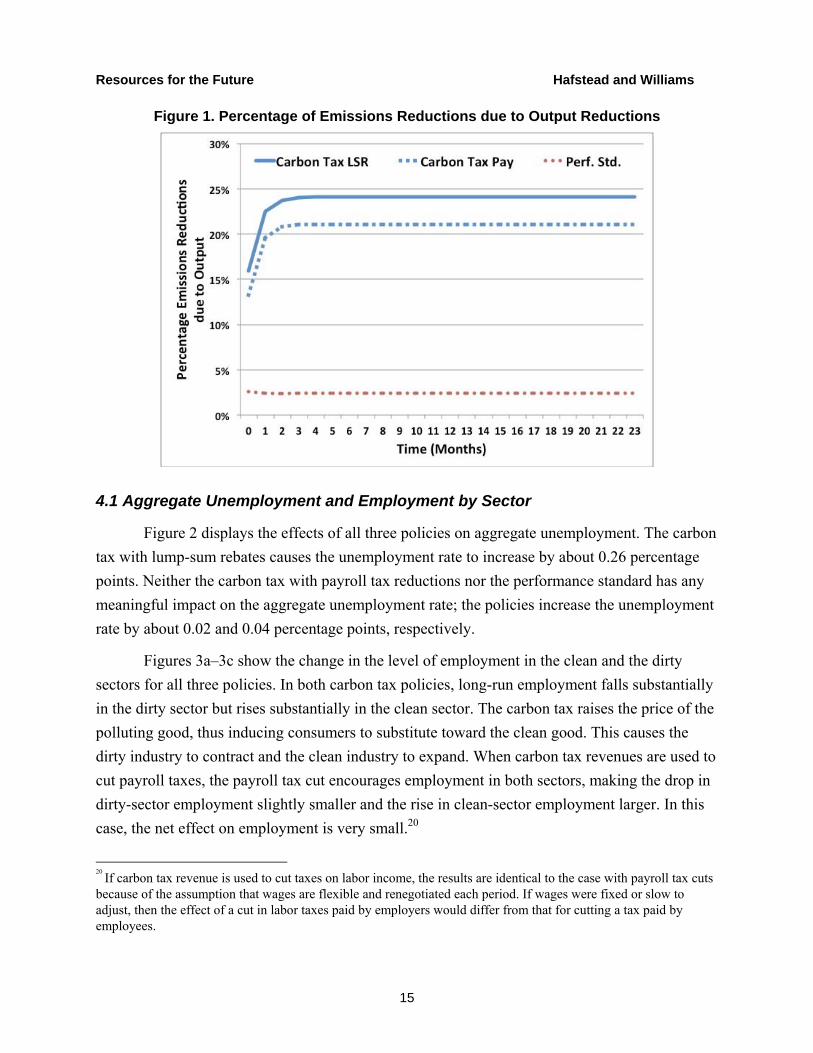
Figure 1 displays the percentage of emissions reductions that can be attributed to output

reductions. Carbon taxes use both channels of emissions reductions, with 21–24 percent of

emissions reductions due to output reductions in the dirty sector. Roughly 2 percent of emissions

reductions in the performance standard policy come from output reductions. Because the carbon

taxes equalize marginal costs across both channels for reducing emissions, they have lower direct

costs of reducing emissions than the performance standard. However, as is shown in the next

section, the much larger dirty-sector output reductions under the carbon tax imply a large labor-

force shift between sectors.

18

The emissions reductions are slightly less in the payroll tax reduction emissions tax policy because the tax cut stimulates economic activity.

19 See Goulder et al. (2016) for further discussion of this difference in incentives between taxes and intensity

standards and its economic implications.


15

Figure 1. Percentage of Emissions Reductions due to Output Reductions

4.1 Aggregate Unemployment and Employment by Sector

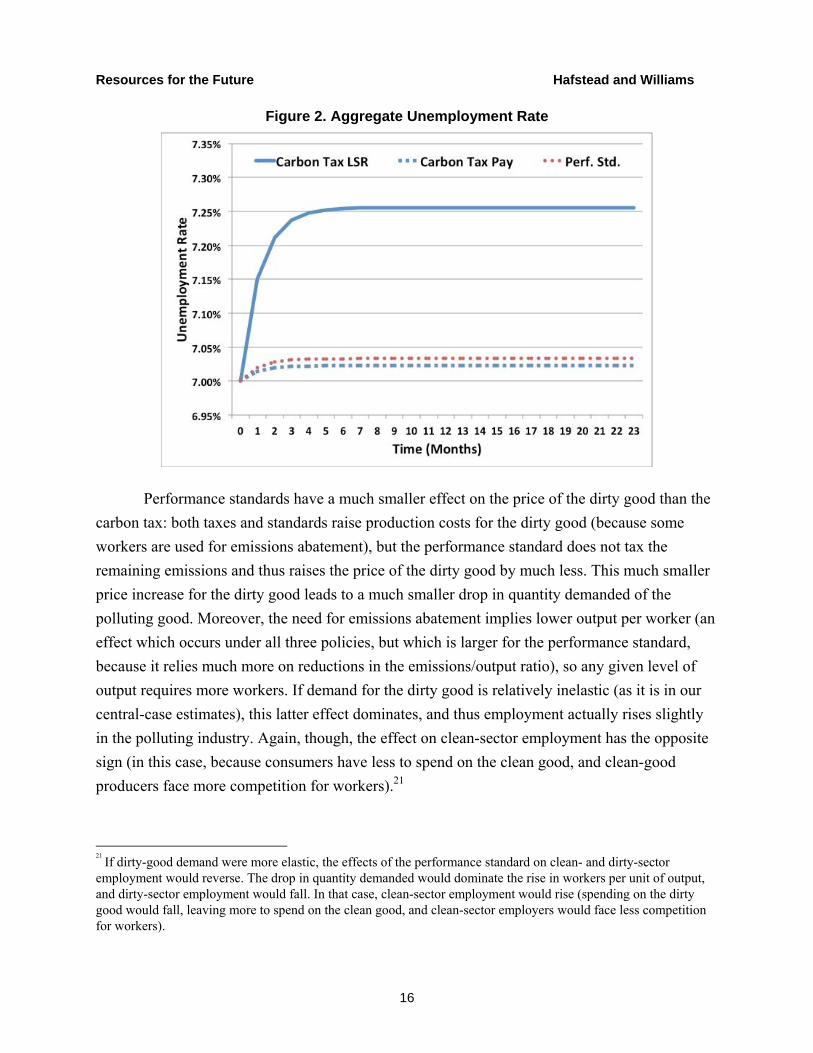
Figure 2 displays the effects of all three policies on aggregate unemployment. The carbon

tax with lump-sum rebates causes the unemployment rate to increase by about 0.26 percentage

points. Neither the carbon tax with payroll tax reductions nor the performance standard has any

meaningful impact on the aggregate unemployment rate; the policies increase the unemployment

rate by about 0.02 and 0.04 percentage points, respectively.

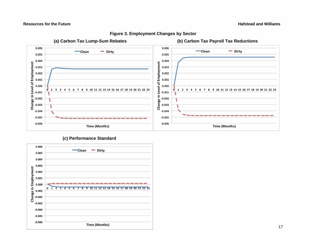
Figures 3a–3c show the change in the level of employment in the clean and the dirty

sectors for all three policies. In both carbon tax policies, long-run employment falls substantially

in the dirty sector but rises substantially in the clean sector. The carbon tax raises the price of the

polluting good, thus inducing consumers to substitute toward the clean good. This causes the

dirty industry to contract and the clean industry to expand. When carbon tax revenues are used to

cut payroll taxes, the payroll tax cut encourages employment in both sectors, making the drop in

dirty-sector employment slightly smaller and the rise in clean-sector employment larger. In this

case, the net effect on employment is very small.20

20 If carbon tax revenue is used to cut taxes on labor income, the results are identical to the case with payroll tax cuts because of the assumption that wages are flexible and renegotiated each period. If wages were fixed or slow to adjust, then the effect of a cut in labor taxes paid by employers would differ from that for cutting a tax paid by employees.


16

Figure 2. Aggregate Unemployment Rate

Performance standards have a much smaller effect on the price of the dirty good than the

carbon tax: both taxes and standards raise production costs for the dirty good (because some

workers are used for emissions abatement), but the performance standard does not tax the

remaining emissions and thus raises the price of the dirty good by much less. This much smaller

price increase for the dirty good leads to a much smaller drop in quantity demanded of the

polluting good. Moreover, the need for emissions abatement implies lower output per worker (an

effect which occurs under all three policies, but which is larger for the performance standard,

because it relies much more on reductions in the emissions/output ratio), so any given level of

output requires more workers. If demand for the dirty good is relatively inelastic (as it is in our

central-case estimates), this latter effect dominates, and thus employment actually rises slightly

in the polluting industry. Again, though, the effect on clean-sector employment has the opposite

sign (in this case, because consumers have less to spend on the clean good, and clean-good

producers face more competition for workers).21

21 If dirty-good demand were more elastic, the effects of the performance standard on clean- and dirty-sector employment would reverse. The drop in quantity demanded would dominate the rise in workers per unit of output, and dirty-sector employment would fall. In that case, clean-sector employment would rise (spending on the dirty good would fall, leaving more to spend on the clean good, and clean-sector employers would face less competition for workers).


17

Figure 3. Employment Changes by Sector

(a) Carbon Tax Lump-Sum Rebates (b) Carbon Tax Payroll Tax Reductions

(c) Performance Standard


18

The net effects depend largely on how the policy shift affects the value of a job match, which

(holding parameters constant) depends on how the real after-tax wage changes. Under the carbon tax

with payroll tax cuts, the carbon tax reduces the real wage (by raising the price of the dirty good),

but the payroll tax cuts offset that effect, leaving the after-tax real wage nearly unchanged. Under the

carbon tax with lump-sum rebates, that offsetting effect is missing, so the real wage falls

significantly. Under the performance standard, there also is no payroll tax cut (indeed, the payroll tax

increases very slightly), but the price increase for the dirty good is much smaller, leading to a

relatively small drop in the real wage.22

There are two key points to take away here. First, under all three policy scenarios, the

employment effects represent much more of a shift in employment—fewer jobs in one sector but

more jobs in the other—rather than a change in overall employment. This is particularly true for the

carbon tax with payroll tax cuts and the performance standard, where the net effect on employment

is very small. Second, the employment shifts are much smaller under the performance standard than

under either carbon tax policy, because the relative output price effects are much smaller under the

performance standard. To the extent that policymakers view industry-level employment contractions

as undesirable—even if they are offset by employment gains elsewhere—this will make performance

standards relatively attractive compared with carbon taxes.

These figures also illustrate the major problem noted earlier with empirical studies that use a

difference-in-differences estimator, with unregulated (i.e., clean) industries as a control group. In our

model, neither carbon taxes nor performance standards directly affect the clean industry, and yet

every policy we consider causes changes in clean-industry employment that are similar in magnitude

to the dirty-industry employment change. A difference-in-differences estimator would take the

difference between the employment changes across the two sectors as an estimate of the effect of

environmental policy. Thus in the tax cases, it would substantially overestimate the job loss in the

dirty sector and overestimate the total job loss by even more.23 In the performance-standard case, it

would find a significant job gain, when the true total effect is a job loss.

22

These effects mirror similar results for taxes versus performance standards from the literature on tax interactions (in models with full employment). See, for example, Goulder et al. (1999) or Fullerton and Metcalf (2001). 23 While our model focuses on clean and dirty industries, the same problem would arise for difference-in-differences estimators more generally whenever the two regulated and unregulated firms’ products are substitutes and labor can move between regulated and unregulated firms.


19

4.2 Labor Market Outcomes

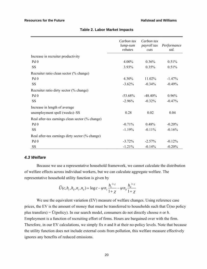
Table 2 displays the impact of the three policies on key labor-market variables in both the

initial period of the policy (Pd 0) and in the long run (SS). As the labor market becomes more slack,

hiring becomes easier; that is, recruiter productivity endogenously increases, making it easier for

matches to occur given a fixed amount of recruitment effort. Under the carbon tax policies,

recruitment initially increases in the clean sector as consumer substitution toward the clean good

induces clean-sector firms to attempt to hire more workers. In the long run, recruitment declines in

the clean sector, despite a larger workforce, because of the increased productivity of recruiters.

In the dirty sector, recruitment falls dramatically in the first period of the carbon tax policies

as the firms reduce hiring below the replacement rate, causing the sector to shrink. But recruitment

does not fall to zero, indicating that firms in the dirty sector decrease employment through slow

hiring and natural attrition, rather than laying off workers.24

Under any of the policy scenarios, there is almost no change in the probability of finding a

job. Even in the lump-sum rebate carbon tax policy, where the change in job-finding probability is

the largest, that change translates into an increase in average unemployment spells of just two days

(compared with seven weeks in the baseline). Furthermore, the job-finding probability is almost flat

across all policies over time, suggesting that workers looking for jobs immediately after the

implementation of the policy spend the same amount of time looking for jobs as those looking for

jobs years after the introduction of the policy.

Earnings in the dirty sector fall immediately after the introduction of environmental policy,

with the drop most pronounced in the carbon tax policies. Workers in the clean sector also face

decreases in earnings, but the initial drop is less severe. Over the longer term, earnings in both

sectors converge to roughly the same level.

24 This matches up with empirical results from Curtis (2012), who found that the drop in employment in regulated industries caused by the NOx budget program occurred primarily through decreased hiring rates rather than increased job separations.


20

Table 2. Labor Market Impacts

Carbon tax lump-sum

rebates

Carbon tax payroll tax

cuts Performance

std.

Increase in recruiter productivity

Pd 0 4.00% 0.36% 0.51%

SS 3.93% 0.35% 0.51%

Recruiter ratio clean sector (% change)

Pd 0 4.30% 11.02% -1.47%

SS -3.62% -0.34% -0.49%

Recruiter ratio dirty sector (% change)

Pd 0 -53.68% -48.40% 0.96%

SS -2.96% -0.32% -0.47%

Increase in length of average

unemployment spell (weeks)–SS 0.28 0.02 0.04

Real after-tax earnings clean sector (% change)

Pd 0 -0.71% 0.48% -0.20%

SS -1.19% -0.11% -0.16%

Real after-tax earnings dirty sector (% change)

Pd 0 -3.72% -2.57% -0.12%

SS -1.21% -0.14% -0.20%

4.3 Welfare

Because we use a representative household framework, we cannot calculate the distribution

of welfare effects across individual workers, but we can calculate aggregate welfare. The

representative household utility function is given by

We use the equivalent variation (EV) measure of welfare changes. Using reference case

prices, the EV is the amount of money that must be transferred to households such that Ū(no policy

plus transfers) = Ū(policy). In our search model, consumers do not directly choose n or h.

Employment is a function of recruiting effort of firms. Hours are bargained over with the firm.

Therefore, in our EV calculations, we simply fix n and h at their no-policy levels. Note that because

the utility function does not include external costs from pollution, this welfare measure effectively

ignores any benefits of reduced emissions.

U(c,hc ,hd ,nc ,nd ) logc nc

hc1

1 nd

hd1

1


21

The welfare costs of the environmental policies are small, as shown in Table 3. The welfare

cost of a $20/ton carbon tax with lump-sum rebates is equivalent to a loss of 0.13 percent of wealth.

When revenues are used to finance payroll tax cuts, the welfare loss is only 0.03 percent of wealth.

As was the case with unemployment, the welfare costs of the performance standard are similar to the

welfare costs of the carbon tax with payroll tax reductions.

Table 3. Welfare

Carbon tax lump-sum

rebates

Carbon tax payroll tax

cuts Performance

std.

EV -$8,692 b -$1,901 b -$2,746 b

EV (as % of wealth) -0.13% -0.03% -0.04%

EV per ton reduced -$46.11 -$10.44 -$14.56

These estimates might understate the cost of job dislocations. Davis and von Wachter (2011)

show that workers who lose their jobs suffer not just a period of unemployment, but also a much

longer-term drop in labor earnings. Our model includes the cost of that unemployment spell, but not

any effect on earnings after a worker is re-employed. However, as noted earlier, we find that the

employment shifts caused by environmental policy in our simulations happen entirely via natural

attrition, rather than layoffs. Moreover, it is unclear how much (if any) of the earnings loss Davis

and von Wachter found represents a social cost, rather than a purely distributional effect.25

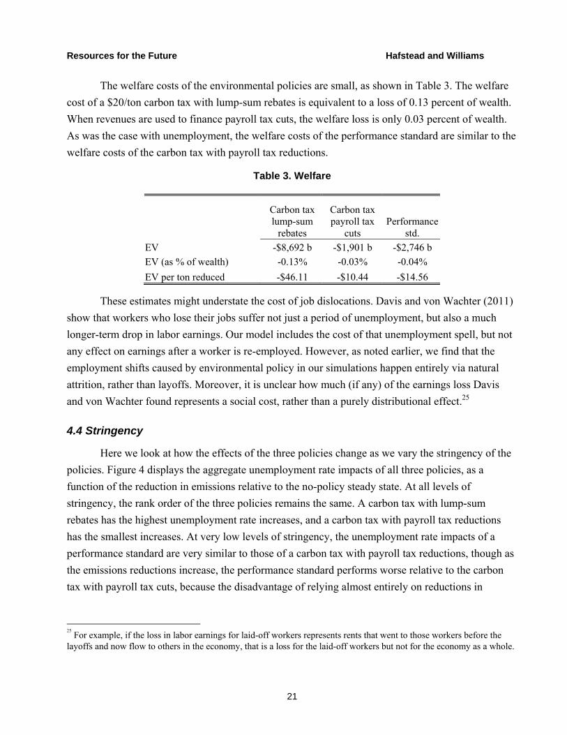
4.4 Stringency

Here we look at how the effects of the three policies change as we vary the stringency of the

policies. Figure 4 displays the aggregate unemployment rate impacts of all three policies, as a

function of the reduction in emissions relative to the no-policy steady state. At all levels of

stringency, the rank order of the three policies remains the same. A carbon tax with lump-sum

rebates has the highest unemployment rate increases, and a carbon tax with payroll tax reductions

has the smallest increases. At very low levels of stringency, the unemployment rate impacts of a

performance standard are very similar to those of a carbon tax with payroll tax reductions, though as

the emissions reductions increase, the performance standard performs worse relative to the carbon

tax with payroll tax cuts, because the disadvantage of relying almost entirely on reductions in

25

For example, if the loss in labor earnings for laid-off workers represents rents that went to those workers before the layoffs and now flow to others in the economy, that is a loss for the laid-off workers but not for the economy as a whole.


22

emissions per unit of output (rather than reducing output from the polluting industry) grows as the

policies become more stringent.

Figure 4. Unemployment Rates by Stringency

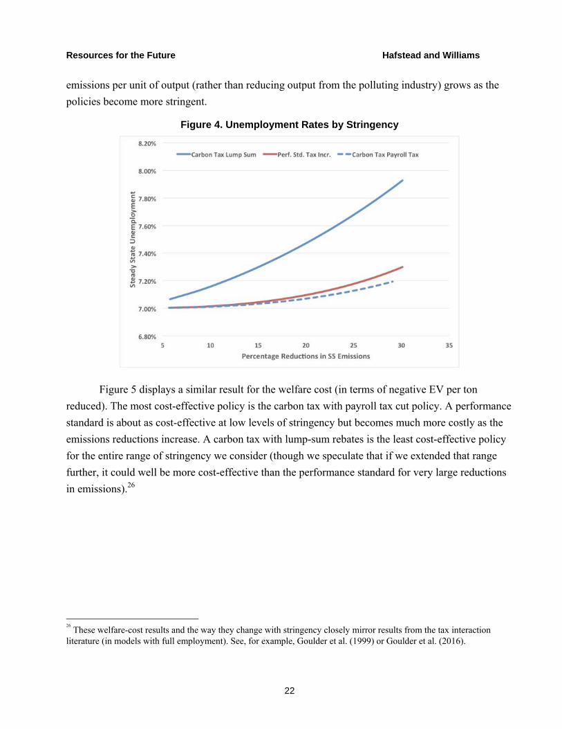
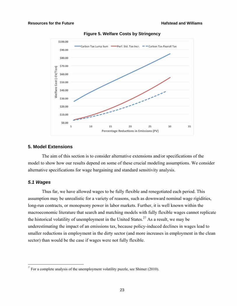
Figure 5 displays a similar result for the welfare cost (in terms of negative EV per ton

reduced). The most cost-effective policy is the carbon tax with payroll tax cut policy. A performance

standard is about as cost-effective at low levels of stringency but becomes much more costly as the

emissions reductions increase. A carbon tax with lump-sum rebates is the least cost-effective policy

for the entire range of stringency we consider (though we speculate that if we extended that range

further, it could well be more cost-effective than the performance standard for very large reductions

in emissions).26

26

These welfare-cost results and the way they change with stringency closely mirror results from the tax interaction literature (in models with full employment). See, for example, Goulder et al. (1999) or Goulder et al. (2016).


23

Figure 5. Welfare Costs by Stringency

5. Model Extensions

The aim of this section is to consider alternative extensions and/or specifications of the

model to show how our results depend on some of these crucial modeling assumptions. We consider

alternative specifications for wage bargaining and standard sensitivity analysis.

5.1 Wages

Thus far, we have allowed wages to be fully flexible and renegotiated each period. This

assumption may be unrealistic for a variety of reasons, such as downward nominal wage rigidities,

long-run contracts, or monopsony power in labor markets. Further, it is well known within the

macroeconomic literature that search and matching models with fully flexible wages cannot replicate

the historical volatility of unemployment in the United States.27 As a result, we may be

underestimating the impact of an emissions tax, because policy-induced declines in wages lead to

smaller reductions in employment in the dirty sector (and more increases in employment in the clean

sector) than would be the case if wages were not fully flexible.

27

For a complete analysis of the unemployment volatility puzzle, see Shimer (2010).


24

To investigate the impact of flexible wages on our results, we consider staggered wage

bargaining as in Gertler and Trigari (2009). To do this, we introduce a continuum of firms in each sector. Firms are identical in each sector. Each period, a firm has a fixed probability 1 – that it may

renegotiate its wage contract.28 The adjustment probability is independent over time, and although the length of contract is indeterminate, the average contract will last periods. We follow

Gertler and Trigari and assume that all workers at a given firm receive the same wage. Given the

Poisson adjustment and common-within-firm wage assumption, we can write the average wage in

each sector as a function of an optimal target wage (which takes into consideration that the wage

may be fixed for a lengthy period) and the average wage in the previous period.29

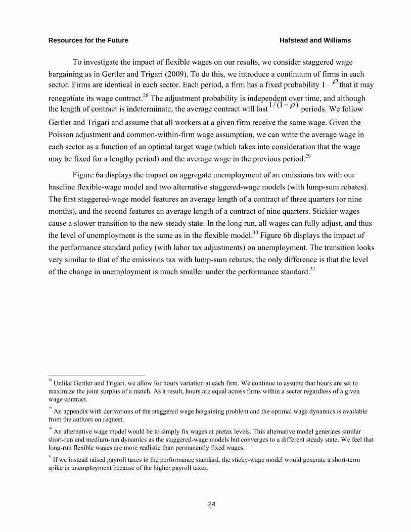
Figure 6a displays the impact on aggregate unemployment of an emissions tax with our

baseline flexible-wage model and two alternative staggered-wage models (with lump-sum rebates).

The first staggered-wage model features an average length of a contract of three quarters (or nine

months), and the second features an average length of a contract of nine quarters. Stickier wages

cause a slower transition to the new steady state. In the long run, all wages can fully adjust, and thus

the level of unemployment is the same as in the flexible model.30 Figure 6b displays the impact of

the performance standard policy (with labor tax adjustments) on unemployment. The transition looks

very similar to that of the emissions tax with lump-sum rebates; the only difference is that the level

of the change in unemployment is much smaller under the performance standard.31

28

Unlike Gertler and Trigari, we allow for hours variation at each firm. We continue to assume that hours are set to maximize the joint surplus of a match. As a result, hours are equal across firms within a sector regardless of a given wage contract. 29

An appendix with derivations of the staggered wage bargaining problem and the optimal wage dynamics is available from the authors on request. 30

An alternative wage model would be to simply fix wages at pretax levels. This alternative model generates similar short-run and medium-run dynamics as the staggered-wage models but converges to a different steady state. We feel that long-run flexible wages are more realistic than permanently fixed wages. 31 If we instead raised payroll taxes in the performance standard, the sticky-wage model would generate a short-term spike in unemployment because of the higher payroll taxes.

1/ (1 )


25

Figure 6. Aggregate Unemployment and Sticky Wages

(a) Carbon Tax Lump-Sum Rebates

(b) Performance Standard

The flexible- and sticky-wage models differ significantly in how the aggregate

unemployment rate responds to changes in labor and payroll taxes. In particular, in the flexible-wage

model, changes to labor and payroll taxes have the same unemployment impact because the wage


26

can simply be negotiated to deliver the optimal take-home pay. When wages are fixed, even

temporarily (as in the staggered-wage model), this is no longer true. A cut in labor income taxes will

increase the take-home pay of the worker but will have no impact on the pretax wage paid by the

employer. A reduction in employer payroll taxes, however, will decrease the net-of-tax payroll cost

for the employer. This reduction in worker costs will increase the value of new hires to the firm,

leading to a direct increase in both recruiting and jobs, relative to no payroll tax cut. These

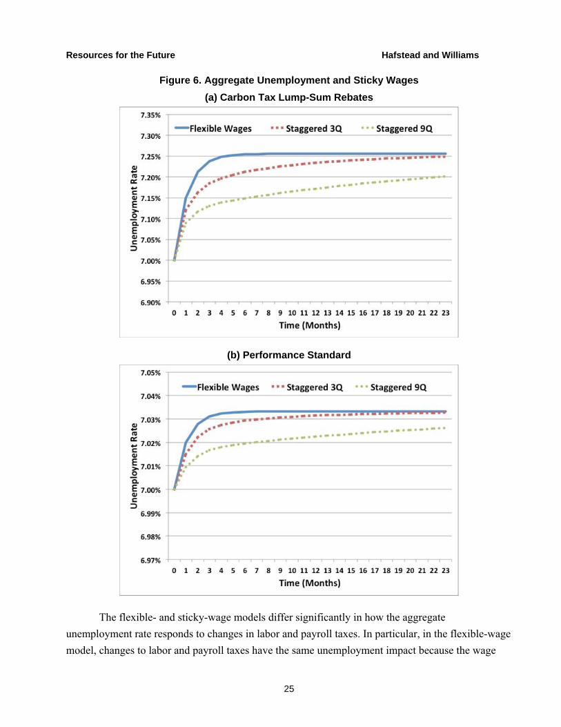
differences can be seen in Figure 7, which shows the response of aggregate unemployment to an

emissions tax when revenues are recycled through either labor or employer payroll tax reductions in

the three-quarter staggered-wage model.32 While both revenue-recycling measures lead to the same

long-run unemployment rate very slightly above 7 percent (the same as in the flexible-wage model

with revenue recycling), employer payroll tax reductions lead to a dramatically different transition as

unemployment falls sharply by three months after the implementation of the emissions tax and

payroll tax cut before slowly increasing over time.33

Figure 7. Aggregate Unemployment and Revenue-Recycling: 3Q Staggered Wage Model

32

As in the flexible wage case, we consider a onetime permanent reduction in taxes such that the policy is fully revenue-neutral over the infinite horizon. 33

This result may appear in part because our model allows employer recruitment effort to vary, but not workers’ search effort. Thus making a successful job match more valuable to employers leads to more hiring (because employers respond by increasing recruiting effort), but making a successful match more valuable to employees causes no such effect.


27

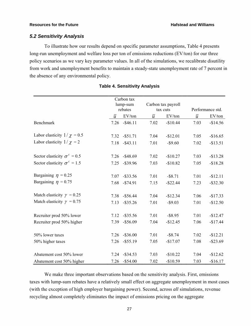
5.2 Sensitivity Analysis

To illustrate how our results depend on specific parameter assumptions, Table 4 presents

long-run unemployment and welfare loss per ton of emissions reductions (EV/ton) for our three

policy scenarios as we vary key parameter values. In all of the simulations, we recalibrate disutility

from work and unemployment benefits to maintain a steady-state unemployment rate of 7 percent in

the absence of any environmental policy.

Table 4. Sensitivity Analysis

Carbon tax lump-sum

rebates Carbon tax payroll

tax cuts Performance std.

u EV/ton u EV/ton u EV/ton

Benchmark 7.26 -$46.11 7.02 -$10.44 7.03 -$14.56

Labor elasticity 1 / = 0.5 7.32 -$51.71 7.04 -$12.01 7.05 -$16.65Labor elasticity 1 / = 2 7.18 -$43.11 7.01 -$9.60 7.02 -$13.51

Sector elasticity c = 0.5 7.26 -$48.69 7.02 -$10.27 7.03 -$13.28

Sector elasticity c = 1.5 7.25 -$39.96 7.03 -$10.82 7.05 -$18.28

Bargaining = 0.25 7.07 -$33.56 7.01 -$8.71 7.01 -$12.11Bargaining = 0.75 7.68 -$74.91 7.15 -$22.44 7.23 -$32.30

Match elasticity = 0.25 7.38 -$56.44 7.04 -$12.34 7.06 -$17.33Match elasticity = 0.75 7.13 -$35.26 7.01 -$9.03 7.01 -$12.50

Recruiter prod 50% lower 7.12 -$35.56 7.01 -$8.95 7.01 -$12.47

Recruiter prod 50% higher 7.39 -$56.09 7.04 -$12.45 7.06 -$17.44

50% lower taxes 7.26 -$36.00 7.01 -$8.74 7.02 -$12.21

50% higher taxes 7.26 -$55.19 7.05 -$17.07 7.08 -$23.69

Abatement cost 50% lower 7.24 -$34.53 7.03 -$10.22 7.04 -$12.62

Abatement cost 50% higher 7.26 -$54.00 7.02 -$10.59 7.03 -$16.17

We make three important observations based on the sensitivity analysis. First, emissions

taxes with lump-sum rebates have a relatively small effect on aggregate unemployment in most cases

(with the exception of high employer bargaining power). Second, across all simulations, revenue

recycling almost completely eliminates the impact of emissions pricing on the aggregate


28

unemployment rate. Third, while the performance standard is always more costly than the carbon tax

with payroll tax cuts, the unemployment rate of the performance standard is only slightly higher than

the unemployment rate of the carbon tax with payroll tax cut policy.

For the simulations of the carbon tax with lump-sum revenue recycling, the effect of

parameter values on long-run unemployment is consistent with our priors. The long-run

unemployment impact is decreasing in the elasticity of labor supply. If workers are more willing to

change their hours of work, more of the adjustment will be on the intensive margin, and thus less is

needed on the extensive margin. Unemployment impacts of emissions taxes are largely independent

of the elasticity of substitution between the two sectors in consumption; welfare cost per ton, on the

other hand, decreases as the elasticity increases (making it easier to substitute from dirty to clean

goods).

Bargaining power determines whether the firms or the workers bear a larger share of the incidence of the emissions tax. If employees have more bargaining power ( 0.5 )—in other

words, they get a larger share of the surplus from a job match—then they also bear more of the

burden of the tax. Thus employers’ incentive to hire drops by less, and consequently the impact on unemployment is smaller. The opposite is true if employers have more bargaining power ( 0.5 ).

Changing the elasticity in the match functions changes the number of job matches that will be

created for a given increase in recruiting effort. Decreasing the elasticity decreases the ability of the

clean sector to hire workers who lost jobs in the dirty sector. As a result, the unemployment impact

is decreasing in the match elasticity.

Increasing the steady-state recruiter productivity increases the long-run unemployment effect

of any given environmental policy. The higher the recruiter productivity, the more any given change

in the steady-state value of a job match will affect the steady-state level of unemployment (because

with higher recruiter productivity, recruiting costs are lower, and thus it requires a larger change in

labor-market tightness to offset any given change in the value of a match).

The higher the preexisting tax rate on labor, the larger is the welfare cost under each of the

three policy scenarios (consistent with many results from full-employment models in the prior

literature). The effect of a carbon tax with lump-sum rebates on unemployment is independent of the

level of preexisting taxes, but the effect on unemployment is significantly larger under either the

carbon tax with payroll tax cuts or the performance standard. All three policies cause the economy to

contract slightly, which shrinks the tax base for the labor tax, thus reducing labor tax revenue (and

the larger the preexisting labor tax, the bigger that drop is). Under the carbon tax with payroll tax

cuts or the performance standard, the bigger that drop in revenue, the higher the payroll tax rate will

be (because either the payroll tax cut is smaller or the increase is larger), so a larger preexisting labor


29

tax implies a larger rise in unemployment. Under the carbon tax with lump-sum rebates, that simply

means smaller lump-sum rebates, which leave unemployment largely unaffected.

As explained previously, a difference-in-differences estimator that assumes regulation does

not affect clean sector employment would estimate the employment effect of an emissions tax as dd nd nc when the true effect on the dirty sector is nd and the true total effect is

u nd nc . Notice that the dd estimate is equal to the true impact if and only if there is no

employment change in the clean sector. That assumption is false in our simulations. Table 5 shows the values of dd and u in the benchmark scenario and the sensitivity scenarios, as well as the

ratio of overestimation dd / u . This ratio is useful both as a measure of how misleading a dd

estimator would be and also as a measure of how large the labor reallocation effect of the policy is

relative to the net change in employment.

Table 5. Overestimation of Aggregate Unemployment Effects

Carbon tax lump-sum rebates

Carbon tax payroll tax cuts Performance std.

u dd Ratio u dd Ratio u dd Ratio

Benchmark 0.255 0.788 3.09 0.023 0.930 40.98 0.033 -0.059 -1.77

Labor elasticity 1 / = 0.5 0.317 0.752 2.37 0.035 0.925 26.79 0.050 -0.065 -1.29Labor elasticity 1 / = 2 0.180 0.831 4.62 0.014 0.932 67.54 0.020 -0.059 -2.87

Sector elasticity c = 0.5 0.257 0.456 1.77 0.021 0.599 28.57 0.028 -0.071 -2.51

Sector elasticity c = 1.5 0.251 1.772 7.07 0.028 1.910 68.69 0.049 0.022 0.45

Bargaining = 0.25 0.071 0.888 12.59 0.005 0.928 196.48 0.007 -0.068 -9.89Bargaining = 0.75 0.682 0.532 0.78 0.149 0.857 5.77 0.227 -0.166 -0.73

Match elasticity = 0.25 0.375 0.715 1.91 0.040 0.919 22.99 0.059 -0.074 -1.26Match elasticity = 0.75 0.130 0.865 6.63 0.010 0.938 94.89 0.014 -0.047 -3.28

Recruiter prod 50% lower 0.116 0.867 7.47 0.008 0.932 112.04 0.012 -0.059 -4.78

Recruiter prod 50% higher 0.385 0.711 1.85 0.042 0.920 21.88 0.062 -0.072 -1.16

50% lower taxes 0.255 0.788 3.09 0.014 0.935 68.03 0.020 -0.051 -2.53

50% higher taxes 0.255 0.788 3.09 0.053 0.911 17.20 0.077 -0.084 -1.09

Abatement cost 50% lower 0.244 0.733 3.00 0.030 0.863 28.29 0.039 -0.068 -1.76

Abatement cost 50% higher 0.260 0.812 3.12 0.044 0.959 49.53 0.031 -0.055 -1.77


30

In all scenarios, there is significant reallocation of labor. Using emissions revenues to cut

payroll taxes makes the drop in employment in the dirty sector smaller and the gain in the clean

sector larger, decreasing the actual increase in unemployment but increasing the difference-in-

differences estimate. As a result, a dd estimator would dramatically overestimate the employment

impacts of an emissions tax coupled with revenue-neutral payroll tax cuts but would be off by much

less (though still by a substantial margin) under the other two policy scenarios. Under the

performance standard, looking only at dirty-sector employment gets the sign of the effect wrong

(because employment rises in the dirty sector but falls by more in the clean sector). In that case, the

dd estimator finds an even larger increase in employment, and thus is even further off.

The dd / u ratio is increasing in the labor supply elasticity, the elasticity of substitution

between sector goods, and the match elasticity. The ratio is decreasing in bargaining power and

recruiter productivity.

The dd / u ratio is weakly declining in the stringency of the policy. At a carbon tax of only

$5 per ton with the lump-sum rebates, the ratio is 3.37; at a tax of $80 per ton with lump-sum

rebates, the ratio is 2.37. Hence, the dd estimator overestimates the true employment impact

regardless of policy stringency.

6. Conclusions

This paper used a simple two-sector general-equilibrium model with job search frictions to

look at how environmental policies affect employment by sector and aggregate unemployment. It

found that while imposing an environmental tax causes a substantial drop in employment in the

polluting sector of the economy, it also indirectly causes an increase in employment in the

nonpolluting sector. Thus the effect is primarily a shift of employment between sectors; the net

effect on total employment (and unemployment) is small. And that net effect is even smaller if

revenues from the tax are used to finance reductions in payroll taxes. An environmental performance

standard results in a much smaller shift in employment between industries, though the net effect on

employment is slightly larger than under a pollution tax with revenue recycled to cut payroll taxes.

These results suggest that overall effects on unemployment should not be a substantial factor

in the evaluation of environmental policy. These effects are small and likely to be greatly

outweighed by the other effects of the policy. However, because emissions taxes cause substantial

sectoral shifts in employment, those effects could matter—and to the extent that the shifts are

undesirable, that may provide a rationale for using performance standards (or other intensity-

standard policies) rather than emissions taxes.


31

The results also suggest a need for caution in drawing lessons from partial-equilibrium

empirical studies of the effects of environmental regulation. Such studies might accurately estimate

the effects on the regulated industry, but not the effects on the rest of the economy, which our results

suggest will be of roughly equal and opposite magnitude. Ignoring those effects and interpreting the

estimated effect for the regulated industry as an estimate for the whole economy will thus lead to a

drastic overestimate of the total effect (indeed, it could get the sign of that total effect wrong).

This problem is even more serious for difference-in-difference studies that use unregulated

sectors as a control group: the rise in employment in those sectors will be mistakenly interpreted as a

larger drop in employment in the regulated sectors.34

However, this is not to say that those partial-equilibrium empirical studies are useless.

Indeed, they could provide highly valuable information about the employment effects of regulation,

as long as they are interpreted correctly (as the effect on the regulated sector or as the difference in

effects between regulated and unregulated sectors). Taken together with a model like ours, such an

estimate could be highly valuable.

The general framework developed in this paper opens up many potential directions for future

research. Perhaps the most interesting of these is whether environmental policy should vary across

different stages of the business cycle, and if so, how. Suppose the government decides that a new

environmental regulation is needed, but it reaches that decision during a major recession. Does it

make sense to impose that new regulation immediately, or is it better to wait until after an economic

recovery is well under way?

Another potential direction is to look at how unemployment changes the distributional effects

of regulation. Even though unemployment has little influence on the aggregate welfare effects, it

may have substantial distributional effects: workers in clean industries could be made substantially

better off, while workers in dirty industries suffer. This would require a more disaggregated analysis,

34 These papers often note this potential problem. For example, Greenstone (2002, 1212) notes, “Since it is likely that the regulation effects partially reflect some shifting of manufacturing activity within the United States, they probably overstate the national loss of activity due to the nonattainment designations. Moreover, the possibility of intra-country shifting means that the regulation effects are also likely to over-state losses in nonattainment counties.” However, Greenstone then goes on to argue that this problem is likely small. And this caveat is almost always omitted when estimates from these papers are cited and used.


32

as well as adding occupation-specific skills (or switching costs to move between industries), but

would otherwise fit well within the framework developed here.35

The model could also readily be adapted to look at other types of policies. Trade policy is an

obvious example; that is another setting in which employment effects are politically very important

and in which CGE models are frequently used.

The transitions in the model are generally very quick, typically converging to a new steady

state within less than two years. There are many reasons why real-world transitions might be slower,

including the occupation-specific skills or switching costs just mentioned, as well as others such as

capital adjustment costs or effects of work experience. Extending the model to include one or more

of those factors would help add more realism to the transition dynamics.

Finally, it would be useful to empirically test some of the predictions of this model (or of an

extended version of the model, such as the extension to occupation- or sector-specific skills). Clean

identification would be a big challenge for testing many of the model’s predictions, because a key

aspect of the model is its general-equilibrium nature, and general-equilibrium effects are inherently

difficult to identify empirically. Nonetheless, a careful empirical analysis could likely test at least

some of the predictions from the model, and such a test would be quite valuable.

35 Walker (2013) provides an interesting empirical analysis of what happens to workers in newly regulated firms, using a difference-in-difference-in-differences approach (conceptually very similar to Greenstone 2002). This approach has the same potential problem as other analyses using this approach: to the extent that general-equilibrium effects from regulation affect unregulated firms, this will bias the estimates of the effects of regulation. An extension of our model to include occupation- or sector-specific skills could be helpful by indicating how to interpret Walker’s results (indicating the magnitude of the bias from general-equilibrium effects). At the same time, Walker’s estimates could be useful as a way of calibrating that extended model or could serve as an empirical test of some of the predictions of such a model.


33

References

Amaral, P., and M. Tasci. 2013. “The Cyclical Behavior of Equilibrium Unemployment and Vacancies across OECD Countries.” Working paper. Federal Reserve Bank of Cleveland.

Aubert, D., and M. Chiroleu-Assouline. 2015. “Environmental Tax Reform and Income Distribution with Imperfect Heterogeneous Labor Markets.” Working paper. Université Paris 1–Panthéon Sorbonne

Balistreri, E.J. 2002. “Operationalizing Equilibrium Unemployment: A General Equilibrium External Economies Approach.” Journal of Economic Dynamics & Control 26: 347–74.

Berman, E., and L. Bui. 2001. “Environmental Regulation and Labor Demand: Evidence from the South Coast Air Basin.” Journal of Public Economics 79 (2): 265–95.

Blundell, R., L. Pistaferri, and I. Preston. 2008. “Consumption Inequality and Partial Insurance.” American Economic Review 98 (5): 1887–1921.

Bovenberg, A., and F. van der Ploeg. 1996. “Optimal Taxation, Public Goods and Environmental Policy with Involuntary Unemployment.” Journal of Public Economics 62 (1): 59–83.

Curtis, M. 2012. “Who Loses under Power Plant Cap-and-Trade Programs? Estimating the Impact of the NOx Budget Trading Program on Manufacturing Employment.” Working paper. Georgia State University.

Steven J. Davis & Till Von Wachter. 2011. “Recessions and the Costs of Job Loss,” Brookings Papers on Economic Activity, 43(2): 1-72.

Fullerton, D., and G.E. Metcalf. 2001. “Environmental Controls, Scarcity Rents, and Pre-existing Distortions.” Journal of Public Economics 80 (2): 249–67.

Gertler, M., and A. Trigari. 2009. “Unemployment Fluctuations with Staggered Nash Wage Bargaining.” Journal of Political Economy 117 (1): 38–86.

Goulder, Lawrence H., Marc A.C. Hafstead, and Roberton C. Williams III. 2016. “General Equilibrium Impacts of a Federal Clean Energy Standard.” American Economic Journal: Economic Policy (May).

Goulder, Lawrence H., Ian W.H. Parry, Roberton C. Williams III, and Dallas Burtraw. 1999. “The Cost-Effectiveness of Alternative Instruments for Environmental Protection in a Second-Best Setting.” Journal of Public Economics, 1999, 72:329–360

Greenstone, M. 2002. “The Impacts of Environmental Regulations on Industrial Activity: Evidence from the 1970 and 1977 Clean Air Act Amendments and the Census of Manufactures.” Journal of Political Economy 110 (6): 1175–1219.

Hall, R.E. 2005. “Employment Fluctuations with Equilibrium Wage Stickiness.” American Economic Review 98 (4): 1653–74.


34

Hall, R.E., and P.R. Milgrom. 2008. “The Limited Influence of Unemployment on the Wage Bargain.” American Economic Review 98 (4): 1653–74.

Heutel, G. 2012. “How Should Environmental Policy Respond to Business Cycles? Optimal Policy under Persistent Productivity Shocks.” Review of Economic Dynamics 15: 244–64.

Holland, S., J.E. Hughes, and C. Knittel. 2009. “Greenhouse Gas Reductions under Low Carbon Fuel Standards?” American Economic Journal: Economic Policy 1 (1): 106–46.

Merz, M. 1995. “Search in the Labor Market and the Real Business Cycle.” Journey of Monetary Economics 36 (2): 269–300.

Morgenstern, R.D., W.A. Pizer, and J.S. Shih. 2002. “Jobs versus the Environment: An Industry-Level Perspective.” Journal of Environmental Economics and Management 43: 412–36.

Mortensen, D.T., and C.A. Pissarides. 1994. “Job Creation and Job Destruction in the Theory of Unemployment.” Review of Economic Studies 61 (3): 397–415.

Nordhaus, W. 2008. A Question of Balance: Weighing the Options on Global Warming Policies, New Haven, CT: Yale University Press.

Petrongolo, B., and C.A. Pissarides. 2001. “Looking into the Black Box: A Survey of the Matching Function.” Journal of Economic Literature 39 (2): 390–431.

Pissarides, C.A. 1985. “Short-Run Equilibrium Dynamics of Unemployment, Vacancies, and Real Wages.” American Economic Review 101 (6): 2823–43.

Shimer, R. 2005. “The Cyclical Behavior of Equilibrium Unemployment and Vacancies.” American Economic Review, 95 (1): 25–49.

———. 2010. Labor Markets and Business Cycles. Princeton, NJ: Princeton University Press.

———. 2013. “A Framework for Valuing the Employment Consequences of Environmental Regulation.” Working paper. University of Chicago.

Silva, J.I., and M. Toledo. 2009. “Labor Turnover Costs and the Cyclical Behavior of Vacancies and Unemployment.” Macroeconomic Dynamics 13(Supplement 1): 79–96.

Smith, A., W. Gans, and M. Yuan. 2013. Estimating Employment Impacts of Regulation: A Review of EPA’s Methods for Its Air Rules. Washington, DC: NERA Economic Consulting.

Walker, W. Reed. 2013. “The Transitional Costs of Sectoral Reallocation: Evidence from the Clean Air Act and the Workforce.” Quarterly Journal of Economics 128 (4): 1787–1835.

Yedid-Levi, Y. 2013. “Why Does Employment in All Major Sectors Move Together over the Business Cycle?” Working paper. University of British Columbia.

Documents

Unemployment and Environmental Regulation in General ... · Resources for the Future Hafstead and Williams 1 Unemployment and Environmental Regulation in General Equilibrium Marc