Embed Size (px)
Citation preview

Unified Position Sensorless Solution with Wide
Speed Range Capabilities for IPM Synchronous
Motor Drives

UNIFIED POSITION SENSORLESS SOLUTION WITH WIDE
SPEED RANGE CAPABILITIES FOR IPM SYNCHRONOUS
MOTOR DRIVES
BY
YINGGUANG SUN, B.Sc., M.Sc.
a thesis
submitted to the department of electrical & computer engineering
and the school of graduate studies
of mcmaster university
in partial fulfilment of the requirements
for the degree of
Doctor of Philosophy
c© Copyright by Yingguang Sun, December 2016
All Rights Reserved

Doctor of Philosophy (2016) McMaster University
(Electrical & Computer Engineering) Hamilton, Ontario, Canada
TITLE: Unified Position Sensorless Solution with Wide Speed
Range Capabilities for IPM Synchronous Motor Drives
AUTHOR: Yingguang Sun
M.Sc. in Electrical Engineering
Illinois Institute of Technology, Chicago, US
B.Sc. in Electrical Engineering
Hebei University of Technology, Tianjin, China
SUPERVISOR: Dr. Ali Emadi, Fellow IEEE,
Canada Excellence Research Chair in Hybrid Powertrain
Director, McMaster Institute for Automotive Research
and Technology (MacAUTO), McMaster University
CO-SUPERVISOR: Dr. Shahin Sirouspour, Professor, Department of Elec-
trical and Computer Engineering, McMaster University
NUMBER OF PAGES: xxiv, 167
ii

To My Father, Qi Sun,
My Mother, Li Zhao,
My Wife, Xiaoying Wang.

Abstract
This thesis presents a unified nonlinear optimization based speed and position estima-
tion method in position sensorless control of interior permanent magnet synchronous
motor (IPMSM) drives at wide speed range including standstill.
The existing electromotive force (EMF) based sensorless methods are suitable for
medium and high speed operation, but they can’t be applied at low speed and stand-
still condition due to the reduced EMF values. The conventional saliency tracking
based sensorless methods usually employ the continuous voltage or current injection
at low speed including standstill condition. However, these methods degrade at high
speed by introducing higher loss and torque ripples caused by the injection. Addition-
ally, the initial rotor position needs to be detected at the machine startup to avoid
the reverse rotation and to guarantee the delivery of the expected torque. Therefore,
different position estimation techniques need to be combined in the controller at wide
speed range, which increases the control system complexity.
Hence, a unified nonlinear optimization based speed and position estimation method
is proposed. At startup and standstill conditions, three steps are employed for initial
position estimation. Step I employs pulse voltage injection in the stationary reference
frame and a cost function which contains the knowledge of initial rotor position. The
rotor position can be estimated by minimizing the cost function with injected voltage
iv
and induced current. Since the estimation results in Step I have an ambiguity of 180,
a generalized approach to magnetic polarity detection which exploits asymmetries in
machine specific differential inductance profiles is employed as Step II. In order to im-
prove the estimation accuracy, continuous sinusoidal voltage is injected in estimated
rotor reference frame in Step III. A modified cost function is minimized based on the
injected voltage and resulting current. At running state, cost functions which employ
both speed and position as decision variables are proposed and utilized for estimation.
The speed and position estimation can be delivered by minimizing the proposed cost
functions based on the measurements of the stator voltage and current. Since only
one position estimator exists in the drive system, the speed and position estimation
is unified at wide speed range. The feasibility of the proposed estimation algorithms
is validated with the prototype 5 KW IPMSM drives test bench.
In order to benchmark the proposed estimation method, the performance of the
proposed method was compared with existing sensorless control methods on the same
prototype IPMSM drives test bench. Under the same test conditions, the proposed
method outperforms with improved transient performance and steady state accuracy.
Moreover, the proposed method is capable of delivering estimation with different
voltage injection types and involving the nonlinear motor parameters, which makes
this method more flexible in practice. Additionally, the capability of estimating speed
and position with low sampling frequency also makes the application of the proposed
method promising in high power AC motor drive systems.
v

Acknowledgements
First of all, I would like to express my sincere gratitude to my supervisor, Dr. Ali
Emadi for offering me an opportunity to work in a research group with so many bril-
liant people who have super enthusiasm in providing new knowledge to the electrical
engineering industry. It is him who make it possible for me to be involved in many
high level industrial projects which help me grow up as an electrical engineer and a
researcher. Thanks for all his guidance, suggestion and encouragement.
I am also indebted to Dr. Shahin Sirouspour, who co-supervised my Ph.D. work
during the past three years. He gave me numerous insights when I was not clear about
the research direction at the beginning of my Ph.D. His cautious attitude towards
study and research will be the criterion for me to evaluate my research and work in
the future.
I would like to express my appreciation to Dr. Matthias Preindl as well. To me, he
is like a teacher as well as a good friend. I will never forget the time we spent together
in developing new ideas and solutions to the problems I encountered. Thanks for all
his patience, suggestions and support.
I also would like to express my gratitude to Dr. Babak Nahid-Mobarakeh and Dr.
Mohamed Bakr for being my supervisory committee. Thanks for all the suggestions
they gave me during the committee meetings.
vi

Moreover, this research was undertaken, in part, thanks to funding from the
Canada Excellence Research Chairs Program.
I am also grateful to my friends and lab colleagues, Jing Guo, Ran Gu, Michael
Eull, Berker Bilgin, Fei Peng, Deqiang Wang, Weisheng (James) Jiang, Hao Ge, Yu
Miao, Shamsuddeen Nalakath, Alan Callegaro, Ben Danen, Michael Kasprzak and
Romina Rodriguez, etc. I will never forget the great time I spent with them. I
sincerely hope they will obtain great achievements in their future career.
I am at the dearth of words to express my gratitude and love to my parents for
their endless support and generous love in the past 28 years. I feel sorry for not being
with them for the past a few years. The have sacrificed so much in order to support
my study. Without their selfless love and support, I will never achieve what I have.
At last, I want to show my deepest love to my wife, Xiaoying Wang. We knew each
other when I came to Canada three years ago and she has been always accompanied
with me since then. It is her endless love that encourages me to overcome any difficulty
I met in my life. Thanks for supporting me unconditionally and I will always love her
with all my heart.
vii

Notation and abbreviations
d-q frame Rotor reference frame
α-β frame Stationary reference frame
δ-γ frame Estimated rotor reference frame
θ Rotor position
θ Estimated rotor position
θ Position estimation error
uabc Three-phase voltages
udq Voltages in rotor reference frame
uαβ Voltages in stationary reference frame
uδγ Voltages in estimated rotor reference frame
iabc Three-phase currents
idq Currents in rotor reference frame
iαβ Currents in stationary reference frame
iδγ Currents in estimated rotor reference frame
λdq Flux linkages in rotor reference frame
λpm Permanent magnet flux linkage
Rs Phase resistance
ωe Synchronous speed
viii

ωe Estimated synchronous speed
Ldq Inductances in rotor reference frame
`dd(idq(t)
)d axis differential self-inductance profile
`qq(idq(t)
)q axis differential self-inductance profile
`dq(idq(t)
)d axis differential cross-coupling inductance profile
`qd(idq(t)
)q axis differential cross-coupling inductance profile
Cαβ Clark transformation
Tdq Park transformation
Te Electromagnetic torque
p Differential operator
P Number of pole pairs
Vdc DC linkage voltage
Eext Extended EMF
eδγ Extended EMFs in estimated rotor reference frame
Ldiffδ Calculated differential inductance
Gi Cost function used in Step I
Gl Cost function used in Step III and low speed
Gr Cost function used for medium and high speed
J Partial derivative of the cost function
H Hessian of the cost function
IPMSM Interior Permanent Magnet Synchronous Machine
IPM Interior Permanent Magnet
PMSM Permanent Magnet Synchronous Machine
FOC Field Oriented Control
ix

DTC Direct Torque Control
EMF Electromotive Force
DC Direct Current
AC Alternating Current
VSI Voltage Source Inverter
IGBT Insulated Gate Bipolar Transistor
MOSFET Metal-Oxide-Semiconductor-Field Effect Transistor
PLL Phase Locked Loop
MTPA Maximum Torque-per-ampere
PWM Pulse Width Modulation
SPWM Sinusoidal Pulse Width Modulation
SVPWM Space Vector Pulse Width Modulation
LPF Low-pass Filter
BPF Band-pass Filter
LUT Look-up Table
UNOP Unified Nonlinear Optimization Based Method
PSVI Pulsating Sinusoidal Voltage Injection Based Method
EEMF Extended EMF Based Method
x

Contents
Abstract iv
Acknowledgements vi
Notation and abbreviations viii
1 Introduction 1
1.1 Motivation . . . . . . . . . . . . . . . . . . . . . . . . . . . . . . . . . 1
1.2 Contributions . . . . . . . . . . . . . . . . . . . . . . . . . . . . . . . 5
1.3 Outline of the Thesis . . . . . . . . . . . . . . . . . . . . . . . . . . . 6
2 Interior Permanent Magnet Synchronous Motor Drives and Control 10
2.1 Introduction . . . . . . . . . . . . . . . . . . . . . . . . . . . . . . . . 10
2.2 Fundamentals of Interior Permanent Magnet Synchronous Motor . . . 11
2.2.1 Stator Voltage Equations . . . . . . . . . . . . . . . . . . . . . 11
2.2.2 Flux, Inductance and Torque . . . . . . . . . . . . . . . . . . 14
2.3 Inverter Control and Pulse Width Modulation . . . . . . . . . . . . . 16
2.4 Position Sensors and Interface . . . . . . . . . . . . . . . . . . . . . . 23
2.4.1 Resolver and Its Interface . . . . . . . . . . . . . . . . . . . . 23
xi

2.4.2 Encoder and Its Interface . . . . . . . . . . . . . . . . . . . . 26
2.5 Control of Interior Permanent Magnet Synchronous Motor . . . . . . 30
2.6 Conclusions . . . . . . . . . . . . . . . . . . . . . . . . . . . . . . . . 34
3 Existing Sensorless Control Methods of IPM Motor Drives 36
3.1 Introduction . . . . . . . . . . . . . . . . . . . . . . . . . . . . . . . . 36
3.2 EMF Based Speed and Position Estimation . . . . . . . . . . . . . . . 37
3.3 Saliency Tracking Based Speed and Position Estimation . . . . . . . . 42
3.4 Speed and Position Estimation at Wide Speed Range . . . . . . . . . 46
3.5 Initial Position Estimation . . . . . . . . . . . . . . . . . . . . . . . . 49
3.5.1 Short Pulse Voltage Injection for Initial Position Estimation . 50
3.5.2 Magnetic Polarity Detection . . . . . . . . . . . . . . . . . . . 53
3.6 Conclusions . . . . . . . . . . . . . . . . . . . . . . . . . . . . . . . . 54
4 Novel Nonlinear IPM Motor Model 57
4.1 Introduction . . . . . . . . . . . . . . . . . . . . . . . . . . . . . . . . 57
4.2 Novel Nonlinear Model of the Prototype IPM Motor . . . . . . . . . . 58
4.2.1 Nonlinear Flux Linkage and Inductance Profiles . . . . . . . . 58
4.2.2 Measurements of the Nonlinear Look-up Tables . . . . . . . . 60
4.2.3 Nonlinear IPM Motor Model with Inverted LUTs . . . . . . . 61
4.3 Experimental Test Bench of Prototype IPM Motor Drives . . . . . . . 65
4.3.1 Silicon Carbide MOSFET Inverter . . . . . . . . . . . . . . . 66
4.3.2 MicroAutoBox II . . . . . . . . . . . . . . . . . . . . . . . . . 67
4.3.3 Dyno Machine Controller . . . . . . . . . . . . . . . . . . . . . 68
4.3.4 High Accuracy Position Sensor . . . . . . . . . . . . . . . . . 69
xii

4.4 Conclusions . . . . . . . . . . . . . . . . . . . . . . . . . . . . . . . . 70
5 Proposed Nonlinear Optimization Based Initial Position Estimation
at Startup and Standstill 71
5.1 Introduction . . . . . . . . . . . . . . . . . . . . . . . . . . . . . . . . 71
5.2 Pulse Voltage Injection for Position Estimation . . . . . . . . . . . . 73
5.3 Generalized Polarity Detection Method . . . . . . . . . . . . . . . . . 78
5.4 Continuous Sinusoidal Voltage Injection for Position Estimation . . . 83
5.5 Simulation Verifications . . . . . . . . . . . . . . . . . . . . . . . . . 85
5.6 Experimental Verifications . . . . . . . . . . . . . . . . . . . . . . . . 88
5.6.1 Experimental Results on Initial Position Estimation . . . . . . 88
5.6.2 Accuracy Comparison Between Pulse Voltage Injection and Con-
tinuous Sinusoidal Injection . . . . . . . . . . . . . . . . . . . 92
5.7 Conclusions . . . . . . . . . . . . . . . . . . . . . . . . . . . . . . . . 92
6 Proposed Nonlinear Optimization Based Speed and Position Esti-
mation at Running State 94
6.1 Introduction . . . . . . . . . . . . . . . . . . . . . . . . . . . . . . . . 94
6.2 Optimization Based Sensorless Algorithm for Medium and High Speed
Operation . . . . . . . . . . . . . . . . . . . . . . . . . . . . . . . . . 96
6.3 Modification of the Cost Function at Low Speed Operation . . . . . . 99
6.4 Variable Magnitudes Sinusoidal Voltage Injection . . . . . . . . . . . 101
6.5 Observer Implementation . . . . . . . . . . . . . . . . . . . . . . . . . 104
6.6 Experimental Verifications . . . . . . . . . . . . . . . . . . . . . . . . 106
6.7 Parameter Sensitivity Analysis . . . . . . . . . . . . . . . . . . . . . . 114
xiii

6.8 Conclusions . . . . . . . . . . . . . . . . . . . . . . . . . . . . . . . . 118
7 Comparative Assessment of the Proposed Sensorless Approach 119
7.1 Introduction . . . . . . . . . . . . . . . . . . . . . . . . . . . . . . . . 119
7.2 Improvements in Initial Position Estimation . . . . . . . . . . . . . . 120
7.2.1 Dynamic Performance in Initial Position Estimation . . . . . . 121
7.2.2 Magnetic Polarity Detection . . . . . . . . . . . . . . . . . . . 122
7.2.3 Involvement of Machine Nonlinearity in Initial Position Esti-
mation . . . . . . . . . . . . . . . . . . . . . . . . . . . . . . . 124
7.3 Improvements in Speed and Position Estimation at Running State . . 127
7.3.1 Dynamic Performance at Low Speed . . . . . . . . . . . . . . 127
7.3.2 Dynamic Performance at High Speed . . . . . . . . . . . . . . 132
7.3.3 Switch Between Low Speed and High Speed . . . . . . . . . . 137
7.4 Capability of Speed and Position Estimation with Multiple Injection
Types . . . . . . . . . . . . . . . . . . . . . . . . . . . . . . . . . . . 140
7.5 Capability of Speed and Position Estimation with Low Sampling Fre-
quency . . . . . . . . . . . . . . . . . . . . . . . . . . . . . . . . . . . 142
7.6 Computational Burden Analysis . . . . . . . . . . . . . . . . . . . . . 146
7.7 Conclusions . . . . . . . . . . . . . . . . . . . . . . . . . . . . . . . . 149
8 Conclusions and Future Work 150
8.1 Conclusions . . . . . . . . . . . . . . . . . . . . . . . . . . . . . . . . 150
8.2 Future Work Suggested . . . . . . . . . . . . . . . . . . . . . . . . . . 152
8.3 Publications . . . . . . . . . . . . . . . . . . . . . . . . . . . . . . . . 153
8.3.1 Journal Papers . . . . . . . . . . . . . . . . . . . . . . . . . . 153
xiv

8.3.2 Conference Papers . . . . . . . . . . . . . . . . . . . . . . . . 154
xv

List of Figures
1.1 The modern electric motor drive system. . . . . . . . . . . . . . . . . 3
2.1 Clark and Park Transformations. . . . . . . . . . . . . . . . . . . . . 12
2.2 Different rotor configurations of PMSM machines. . . . . . . . . . . . 14
2.3 The d-q axes flux paths in PMSMs. . . . . . . . . . . . . . . . . . . . 15
2.4 Voltage Source Inverter. . . . . . . . . . . . . . . . . . . . . . . . . . 17
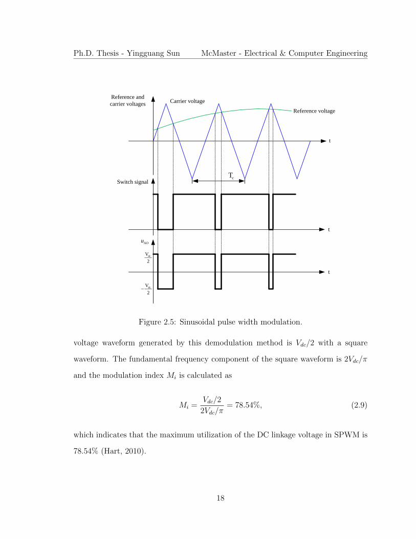
2.5 Sinusoidal pulse width modulation. . . . . . . . . . . . . . . . . . . . 18
2.6 Voltage vectors in SVPWM . . . . . . . . . . . . . . . . . . . . . . . 19
2.7 Switching pattern in Sector I. . . . . . . . . . . . . . . . . . . . . . . 21
2.8 Comparison between SPWM and SVPWM. . . . . . . . . . . . . . . 22
2.9 Resolver and its interface. . . . . . . . . . . . . . . . . . . . . . . . . 24
2.10 Variable reluctance resolver. . . . . . . . . . . . . . . . . . . . . . . . 25
2.11 Speed and position extraction from the resolver interface. . . . . . . . 26
2.12 BEI incremental encoder. . . . . . . . . . . . . . . . . . . . . . . . . . 27
2.13 Absolute and incremental encoders. . . . . . . . . . . . . . . . . . . . 28
2.14 Quadrature output in incremental encoder. . . . . . . . . . . . . . . . 29
2.15 The working theory of the incremental encoder interface. . . . . . . . 30
2.16 Block diagram of the FOC in IPM motor drives. . . . . . . . . . . . . 31
xvi

2.17 Optimal IPM motor operation with voltage and current limits and
torque-speed curve. . . . . . . . . . . . . . . . . . . . . . . . . . . . . 32
3.1 Different reference frames in IPMSM drives. . . . . . . . . . . . . . . 38
3.2 State observer for extended EMF in δ axis. . . . . . . . . . . . . . . . 40
3.3 Extended EMF based position estimator. . . . . . . . . . . . . . . . . 42
3.4 Demodulation based position estimator. . . . . . . . . . . . . . . . . 46
3.5 Linear blending algorithm for speed and position combination. . . . . 48
3.6 Block diagram of the sensorless control system with combined algorithms. 48
3.7 Applied voltage vectors for initial position estimation. . . . . . . . . . 51
3.8 Dual voltage injection based method for magnetic polarity detection. 55
3.9 Framework of the dual voltage pulse injection based method . . . . . 55
4.1 Experimental measured d axis flux linkage profile λd(idq) under differ-
ent id and iq. . . . . . . . . . . . . . . . . . . . . . . . . . . . . . . . 61
4.2 Experimental measured q axis flux linkage profile λq(idq) under different
id and iq. . . . . . . . . . . . . . . . . . . . . . . . . . . . . . . . . . . 62
4.3 Flowchart of look-up table inversion algorithm . . . . . . . . . . . . . 63
4.4 Inverted look-up tables: (a) The inverted profile id(λdq); (b) The in-
verted profile iq(λdq). . . . . . . . . . . . . . . . . . . . . . . . . . . . 64
4.5 Block diagram of the nonlinear machine model dynamics with inverse
LUTs. . . . . . . . . . . . . . . . . . . . . . . . . . . . . . . . . . . . 65
4.6 Prototype IPMSM drives test bench. . . . . . . . . . . . . . . . . . . 66
4.7 Prototype SiC MOSFET inverter. . . . . . . . . . . . . . . . . . . . . 67
4.8 RTI Blockset in Simulink. . . . . . . . . . . . . . . . . . . . . . . . . 68
4.9 Experimental software ControlDesk Next Generation. . . . . . . . . . 69
xvii

5.1 Block diagram of the proposed optimization based initial position es-
timator. . . . . . . . . . . . . . . . . . . . . . . . . . . . . . . . . . . 72
5.2 Screenshot of the scope, voltage injection procedures in initial position
estimation. . . . . . . . . . . . . . . . . . . . . . . . . . . . . . . . . . 73
5.3 Voltage vectors applied for injection in Step I. . . . . . . . . . . . . . 75
5.4 Injected voltages and resulting currents in α-β axes. . . . . . . . . . . 75
5.5 Plot of Gi(θ) versus position estimation errors at different initial posi-
tions for m = 1 based on experimental data. . . . . . . . . . . . . . . 77
5.6 Experimental obtained d axis differential inductance profile `dd(id, 0). 79
5.7 Injected voltages and resulting currents in δ axis for magnetic polarity
detection. . . . . . . . . . . . . . . . . . . . . . . . . . . . . . . . . . 80
5.8 Framework of the proposed polarity detection method. . . . . . . . . 81
5.9 Contour plot of the cost function (5.9) at standstill condition. . . . . 84
5.10 Simulation results on initial position estimation at 41.5: (a) actual
and estimated positions; (b) position estimation error; (c) c1 and c2 in
polarity detection. . . . . . . . . . . . . . . . . . . . . . . . . . . . . 86
5.11 Simulation results on initial position estimation at 250: (a) actual
and estimated positions; (b) position estimation error; (c) c1 and c2 in
polarity detection. . . . . . . . . . . . . . . . . . . . . . . . . . . . . 87
5.12 Simulation results on integration of speed and position estimation at
standstill and low speed: (a) actual and estimated positions; (b) posi-
tion estimation error; (c) actual and estimated speeds. . . . . . . . . 88
xviii
5.13 Experimental results on initial position estimation at 41.5: (a) mea-
sured and estimated positions; (b) position estimation error; (c) c1 and
c2 in polarity detection. . . . . . . . . . . . . . . . . . . . . . . . . . . 89
5.14 Experimental results on initial position estimation at 250: (a) mea-
sured and estimated positions; (b) position estimation error; (c) c1 and
c2 in polarity detection. . . . . . . . . . . . . . . . . . . . . . . . . . . 90
5.15 Experimental results on integration of speed and position estimation
at standstill and running state: (a) measured and estimated positions;
(b) position estimation error; (c) measured and estimated speeds. . . 91
5.16 Experimental results, position estimation errors of pulse voltage injec-
tion and continuous sinusoidal voltage injection. . . . . . . . . . . . . 92
6.1 Block diagram of the proposed nonlinear optimization based sensorless
control system. . . . . . . . . . . . . . . . . . . . . . . . . . . . . . . 95
6.2 Contour plots of the cost function (6.4): (a) 400 rpm and ipeakphase = 0;
(b) 400 rpm and ipeakphase = 4; (c) 800 rpm and ipeakphase = 0. . . . . . . . . 98
6.3 Convex region of the cost function at 400 rpm: (a) convex regions on
the contour plot; (b) zoomed in convex region around the expected
local minimum. . . . . . . . . . . . . . . . . . . . . . . . . . . . . . . 100
6.4 Convex region of the cost function at 800 rpm: (a) convex regions on
the contour plot; (b) zoomed in convex region around the expected
local minimum. . . . . . . . . . . . . . . . . . . . . . . . . . . . . . . 100
6.5 Contour plots of the cost function: (a) cost function Gr at 0 rpm
without injection; (b) cost function Gl at 0 rpm with injection. . . . . 102
xix

6.6 Contour plots of the cost function: (a) cost function Gr at 50 rpm
without injection; (b) cost function Gl at 50 rpm with injection. . . . 102
6.7 Convex regions of the modified cost function Gl: (a) convex region at
0 rpm; (b) convex region at 50 rpm. . . . . . . . . . . . . . . . . . . . 103
6.8 Variable magnitudes voltage injection scheme. . . . . . . . . . . . . . 104
6.9 Nonlinear optimization based position estimator. . . . . . . . . . . . . 105
6.10 Experimental results, convergence tests at standstill condition: (a) pos-
itive initial error; (b) negative initial error. . . . . . . . . . . . . . . . 106
6.11 Experimental results, speed and position estimation before and after
PLL: (a) position estimation at transients; (b) speed estimation. . . . 107
6.12 Experimental results, speed step change without load, 50 rpm: (a)
position estimation error; (b) position estimation at transients; (c)
speed estimation. . . . . . . . . . . . . . . . . . . . . . . . . . . . . . 109
6.13 Experimental results, speed step change with 20% rated torque, 50
rpm: (a) position estimation error; (b) position estimation at tran-
sients; (c) speed estimation . . . . . . . . . . . . . . . . . . . . . . . . 110
6.14 Experimental results, speed step change with 40% rated torque, 50
rpm: (a) position estimation error; (b) position estimation at tran-
sients; (c) speed estimation . . . . . . . . . . . . . . . . . . . . . . . . 111
6.15 Experimental results, speed step change with 40% rated torque, 100
rpm: (a) position estimation error; (b) current in γ axis; (c) position
estimation at transients; (d) speed estimation. . . . . . . . . . . . . . 112
xx

6.16 Experimental results, torque step change at constant speed, 300 rpm:
(a) position estimation error; (b) current in γ axis; (c) position esti-
mation at transients; (d) speed estimation. . . . . . . . . . . . . . . . 113
6.17 Experimental results, wide speed range operation: (a) position estima-
tion error; (b) speed estimation. . . . . . . . . . . . . . . . . . . . . . 114
6.18 Experimental results, speed and position estimation at wide speed
range including standstill: (a) position estimation error; (b) position
estimation at transients; (c) current in γ axis; (d) speed estimation. . 115
6.19 Parameter sensitivity contour plot analysis at 300 rpm with 40% rated
torque: (a) 50% resistance variation; (b) 50% permanent magnet flux
variation; (c) 50% d-q axes inductances variation. . . . . . . . . . . . 116
6.20 Parameter sensitivity experimental test results: (a) ±50% resistance
variation; (b) ±50% PM flux variation; (c) ±50% d-q axes inductances
variation. . . . . . . . . . . . . . . . . . . . . . . . . . . . . . . . . . 117
7.1 The modified PLL used in PSVI and EEMF methods. . . . . . . . . . 120
7.2 Experimental comparison on convergence speed between PSVI method
and UNOP method. . . . . . . . . . . . . . . . . . . . . . . . . . . . 121
7.3 Experimental comparison on torque transient performance between
PSVI method and UNOP method: (a) 20% rated torque change; (b)
40% rated torque change. . . . . . . . . . . . . . . . . . . . . . . . . . 122
7.4 Resulting δ axis currents due to the injection in magnetic polarity
detection. . . . . . . . . . . . . . . . . . . . . . . . . . . . . . . . . . 123
7.5 Plot of Gi(θ) versus position estimation errors at different initial posi-
tions for m = 1 using experimental data. . . . . . . . . . . . . . . . . 124
xxi

7.6 Position estimation errors of the linear method at different initial po-
sitions with different injection durations. . . . . . . . . . . . . . . . . 126
7.7 Position estimation errors of the nonlinear method at different initial
positions with different injection durations. . . . . . . . . . . . . . . . 127
7.8 Estimation accuracy comparison between nonlinear and linear methods
(5Ts for each voltage pulse). . . . . . . . . . . . . . . . . . . . . . . . 128
7.9 Benchmark reference, speed and position estimation with PSVI method
with the same test shown in Figure 6.14: (a) position estimation error;
(b) position estimation at transients; (c) speed estimation. . . . . . . 129
7.10 Experimental results of the UNOP method at low speed, torque step
change at 100 rpm: (a) position estimation error; (b) position estima-
tion at transients; (c) current in γ axis (d) speed estimation. . . . . . 130
7.11 Benchmark reference, PSVI base method at low speed, torque step
change at 100 rpm: (a) position estimation error; (b) position estima-
tion at transients; (c) current in γ axis; (d) speed estimation. . . . . . 131
7.12 Benchmark reference, EEMF base method at high speed, speed step
change with 15% rated torque: (a) position estimation error; (b) posi-
tion estimation at transients; (c) current in γ axis; (d) speed estimation.133
7.13 Experimental results of the UNOP method at high speed, speed step
change with 15% of rated torque: (a) position estimation error; (b)
position estimation at transients; (c) current in γ axis; (d) speed esti-
mation. . . . . . . . . . . . . . . . . . . . . . . . . . . . . . . . . . . 134
xxii

7.14 Benchmark reference, EEMF base method at high speed, torque step
change at 400 rpm: (a) position estimation error; (b) position estima-
tion at transients; (c) current in γ axis; (d) speed estimation. . . . . . 135
7.15 Experimental results of the UNOP method at high speed, torque step
change at 400 rpm: (a) position estimation error; (b) position estima-
tion at transients; (c) current in γ axis; (d) speed estimation. . . . . . 136
7.16 Benchmark reference, the combined method during switch process,
speed step change without load: (a) position estimation error; (b)
position estimation at transients; (c) speed estimation. . . . . . . . . 137
7.17 Experimental results of the proposed unified method during switch
process, speed step change without load: (a) position estimation error;
(b) position estimation at transients; (c) speed estimation. . . . . . . 138
7.18 Benchmark reference, the combined method during switch process,
speed step change with 30% rated torque: (a) position estimation error;
(b) current in γ axis; (c) speed estimation. . . . . . . . . . . . . . . . 139
7.19 Experimental results of the proposed unified method during switch pro-
cess, speed step change with 30% rated torque: (a) position estimation
error; (b) current in γ axis; (c) speed estimation. . . . . . . . . . . . . 140
7.20 Screenshot of the scope, continuous rectangular voltage injection in
Step III. . . . . . . . . . . . . . . . . . . . . . . . . . . . . . . . . . . 141
7.21 Experimental results on initial position estimation at 41.5 with rect-
angular voltage injection: (a) measured and estimated positions; (b)
position estimation error. . . . . . . . . . . . . . . . . . . . . . . . . . 142
xxiii

7.22 Experimental results, speed and position estimation with continuous
rectangular voltage injection: (a) position estimation error; (b) posi-
tion estimation at transients; (c) current in γ axis; (d) speed estimation.143
7.23 Experimental results, speed and position estimation with 2 KHz sam-
pling frequency, no load: (a) position estimation error; (b) position
estimation at transients; (c) speed estimation. . . . . . . . . . . . . . 144
7.24 Experimental results, speed and position estimation with 2 KHz sam-
pling frequency, with 40% rated torque: (a) position estimation error;
(b) position estimation at transients; (c) speed estimation. . . . . . . 145
7.25 Estimation performance validation with different iterations, conver-
gence test with 30 initial error. . . . . . . . . . . . . . . . . . . . . . 147
7.26 Estimation performance validation with different iterations: (a) speed
transients; (b) torque transients. . . . . . . . . . . . . . . . . . . . . . 148
7.27 Sensorless methods comparison. . . . . . . . . . . . . . . . . . . . . . 148
xxiv

Chapter 1
Introduction
1.1 Motivation
The electric machines have been widely used in pumps, fans, aerospace actuators,
robotic actuators and automobile industries. According to the United States Indus-
trial Electric Motor Systems Market Opportunities Assessment published in 1998,
the industrial electric motor systems were the largest single electrical end use in US
economy, which consumed 679 billion kWh power and occupied roughly 23% of all
electricity sold in the United States in 1994 (XENERGY, 1998). Since then the rapid
development of the electric motor systems has been sustained in recent 20 years and
they are currently the single largest electrical end use which accounts for 43% to 46%
of the global electricity consumption (Waide and Brunner, 2011).
The electric machine can be classified into direct current (DC) machines and
alternating current (AC) machines according to the machine input. Compared with
DC machines, AC machines are more commonly employed due to their simplicity and
higher efficiency. The AC machines consist of the stationary part called stator and
1

Ph.D. Thesis - Yingguang Sun McMaster - Electrical & Computer Engineering
the rotating part named rotor. The stator consists of three-phase windings, which
generate the rotating magnetic field. The magnetic field of the rotor is generated by
the rotor windings in induction machines and synchronous machines. However, the
permanent magnets are used as a counterpart of the rotor windings in permanent
magnet synchronous machines (PMSM). Since the rotor field is generated by the
permanent magnets, the motor efficiency improves without rotor copper loss. For a
given output power, the weight and volume are smaller in PMSMs compared with
induction machines or synchronous machines, which leads to a higher power density.
Moreover, less heat is generated in PMSMs for a given power input due to the absence
of rotor windings (Preindl, 2013; Hughes, 2006; Chan, 2002; Nalakath et al., 2015).
In PMSMs, the permanent magnet can either be mounted on the surface of
the rotor core or buried inside the rotor lamination. Compared with the surface
mounted permanent magnet (SPM) machine, the interior permanent magnet (IPM)
synchronous machine has several advantages on the rotor operating characteristics.
Since the permanent magnets are physically installed and protected inside the rotor,
the IPM motor is capable of operating at higher speed robustly than the SPM coun-
terpart. Additionally, the buried permanent magnets change the machine magnetic
circuit and flux linkage path, which leads to the improvements in the electromagnetic
torque production (Jahns et al., 1986; Bilgin et al., 2015).
The proper functioning of the electric machine relies on the electric drive system,
which converts the electric energy into mechanical energy (Emadi, 2014; Preindl,
2013). The modern electric motor drive system shown in Figure 1.1 usually comprises
the power source, the power electronics converter, the electric machine, the mechanical
load and the digital controller. When the electromagnetic torque of the machine
2

Ph.D. Thesis - Yingguang Sun McMaster - Electrical & Computer Engineering
ABC
Electric
machine
DCV
Power electronics
converter
DC power
source
Mechanical load
Digital
controller
Position sensor
Current
measurementPosition sensor
interface
Control
command
Figure 1.1: The modern electric motor drive system.
has the same direction with the machine speed, the power flow direction is positive
(machine consuming energy) and it is called the motor convention. When the machine
torque and speed are in the reverse direction, the power flow direction is negative
(machine generating energy) and the machine operates in the generator convention
(EL-Sharkawi, 2000). In this thesis, the motor convention operation is the sense that
mainly focused on.
In the AC machine drive system, the DC power from the power source needs to
be transformed into AC power for the generation of the rotating magnetic field. This
transformation relies on the voltage source inverter (VSI), which is a specific power
electronics converter used in AC motor drives (Preindl, 2013). The electronic switches,
e.g. Insulated Gate Bipolar Transistor (IGBT) or Metal-Oxide-Semiconductor-Field
Effect Transistor (MOSFET), are controlled by the switching signals provided by the
digital controller. In order to achieve the desired performance, the switching signals
are generated based on the control reference and measurements. The motor speed
3

Ph.D. Thesis - Yingguang Sun McMaster - Electrical & Computer Engineering
or torque are the commonly used control reference while the voltages are the real
quantities that applied on the electric machine. Hence, the reference voltages need to
be determined by the control reference based on the specific control algorithms, e.g.
Field Oriented Control (FOC) and Direct Torque Control (DTC). Those close loop
control algorithms require the feedback of the phase currents and rotor position, which
are normally obtained from the specific current sensors and position sensors. With
the inverted three phase voltages applied on the stator, the electromagnetic torque
can be delivered by the interaction of the stator and rotor fields for the propulsion of
the mechanical load.
The rotor position and speed are indispensable in close loop control and achieving
maximum torque in AC motor drives. The knowledge of position and speed is usually
provided by the specific position sensors (resolver and encoder) in real time. How-
ever, the existence of the position sensor increases the machine size. Moreover, the
position sensor installation requires the shaft extension and frequent maintenance of
the sensors is needed. Besides, the interface between the position sensor output and
controller input is required for signal conditioning, which increases the cost of the en-
tire drive system. Additionally, the motor drive system robustness is degraded due to
the noise issues existed in the signal transmission between the position sensor and the
digital controller, even though specific techniques have been utilized in reducing the
noise in the position sensor interface. Hence, much efforts have been focused on new
methods for position sensorless control of electric motor drives to avoid sensor-related
issues (Sun et al., 2015; Emadi et al., 2008; Fahimi et al., 2004).
The existing sensorless solutions for IPMSM drive system can be divided into two
categories, the electromotive force (EMF) based methods and the saliency tracking
4

Ph.D. Thesis - Yingguang Sun McMaster - Electrical & Computer Engineering
based methods. The EMF based methods work robustly in medium and high speed
while the saliency tracking based method is more suitable for position sensing at low
speed and standstill conditions. For wide speed range operation, different methods
need to be combined, which leads to the existence of at least two different speed and
position estimators in the drive system. In order to reduce the system complexity, a
unified speed and position estimation method for IPMSM drives at wide speed range
is proposed in this thesis. The proposed method estimates speed and position by
minimizing proposed cost functions which contain the position information in the
EMF components as well as in the machine saliency. The feasibility of the proposed
unified position sensing method is validated with the prototype IPMSM drive system.
Besides the capability of providing speed and position information to the drive system
fast and reliably, the proposed method also exhibits several features which will make
it attractive to the adjustable speed drives industry.
1.2 Contributions
The author has contributed a number of original developments in speed and position
estimation of IPM motor drives in this thesis, which are listed as follows:
1. Cost functions based on the voltage equations are proposed for analysis and
implementation of the proposed estimation method.
2. A fast and accurate nonlinear optimization based initial position estimation
method is proposed and validated.
3. An accurate nonlinear IPM motor model with current-flux look-up tables is
proposed and utilized for simulation of the proposed sensorless algorithms.
5

Ph.D. Thesis - Yingguang Sun McMaster - Electrical & Computer Engineering
4. A unified nonlinear optimization based speed and position estimation method
at running state is proposed and validated.
5. Comparative assessments between the proposed methods and the benchmark
references are exhibited for comprehensively evaluating the proposed estimation
methods.
1.3 Outline of the Thesis
This thesis presents a unified speed and position estimation method in position sen-
sorless control of IPMSM drives at wide speed range operation including standstill
condition. The thesis is mainly focused on: (1) Analysis of the proposed cost func-
tions at different operation conditions; (2) Experimental validation of the proposed
sensorless solution at wide speed range; (3) Comparative assessment of the proposed
methods with other existing sensorless methods.
Chapter 2 introduces the components of the modern electric drive system. Firstly,
fundamentals of IPM motors including the generation and interaction of the stator
and rotor flux, the concept of saliency and the torque generation are explained. In
order to generate the rotating flux in the stator, the VSI is employed for converting
DC voltage into AC voltage. The working theory and different control methods of
the VSI are explained. Additionally, the control of AC electric motors requires the
knowledge of speed and position. Therefore the position sensors and their interfaces
are illustrated as well. Moreover, the torque control of IPM motor drives is explained
at the end of this chapter.
Chapter 3 presents the existing sensorless control methods of IPMSM drives. The
6

Ph.D. Thesis - Yingguang Sun McMaster - Electrical & Computer Engineering
EMF based methods which are suitable for medium and high speed operation are
introduced and the extended EMF based estimation method is explained in detail
and implemented in the prototype IPMSM drive system as a benchmark reference.
At low speed including standstill condition, the saliency tracking based methods
which employ the continuous signal injection are introduced. The pulsating voltage
injection method which relies on the high frequency sinusoidal voltage injection in
the estimated rotor reference frame is explained explicitly and is also implemented as
a benchmark reference method. Additionally, the existing initial position estimation
methods at machine startup are also reviewed. Since the initial position estimation
of PMSM usually contains an ambiguity of 180, the conventional magnetic polarity
detection methods in the literature are also studied and presented.
Chapter 4 studies the IPM machine modeling which involves the machine nonlinear
inductance profiles. The traditional nonlinear IPM motor model relies on the flux-
current look-up tables, which requires the differentiation of the flux. A novel nonlinear
machine model which utilizes the current-flux look-up tables is studied and explained
in this chapter. Besides, the components of the prototype IPM motor drive system
including the MicroAutoBox II, the Silicon-Carbide MOSFET inverter and the high
resolution incremental encoder are also briefly presented.
Chapter 5 introduces the proposed initial position estimation method for IPMSM
drives at startup and standstill condition. The initial position estimation has three
steps. Step I employs the voltage pulse injection in the stationary reference frame and
a cost function used in initial position estimation. The rotor position can be estimated
by minimizing the cost function with injected voltage and induced current. Since the
estimation results in Step I have an ambiguity of 180, a generalized approach to
7

Ph.D. Thesis - Yingguang Sun McMaster - Electrical & Computer Engineering
polarity detection which exploits asymmetries in machine specific differential induc-
tance profiles is employed as Step II. In order to improve the estimation accuracy,
continuous sinusoidal voltage is injected in estimated rotor reference frame in Step
III. A modified cost function is minimized based on the injected voltage and resulting
current. The effectiveness of the initial position estimation method is demonstrated
with high accuracy simulation and the prototype IPMSM drives test bench.
Chapter 6 proposes a nonlinear optimization based position and speed estimation
algorithm for wide speed range operations. A cost function which employs both speed
and position as decision variables is proposed and utilized for estimation. The speed
and position can be estimated by minimizing the proposed cost function based on
the measurements of stator voltages and currents. Since the voltage information is
less significant at low speed and unable to be observed at standstill condition, extra
high frequency sinusoidal voltages are injected in estimated magnetic axis. Extra
regularization terms are added in the cost function at low speed to improve speed
and position estimation quality. A phase locked loop (PLL) is involved at the output
of the position estimator serving as a filter. Analysis on the convexity of the proposed
cost functions under different speeds and positions are also presented in this chapter.
The feasibility of the proposed estimation algorithm is validated with the experimental
setup.
Chapter 7 compares the proposed speed and position estimation methods with
the benchmark reference methods mentioned in Chapter 3. The comparisons include
both the dynamic and steady state performance during speed and torque transients
at wide speed range. Besides the comparison, some other attractive features of the
proposed method are also presented in this chapter. Those features include : (1) The
8

Ph.D. Thesis - Yingguang Sun McMaster - Electrical & Computer Engineering
capability of estimating speed and position with multiple voltage injection types;
(2) The capability of involving nonlinear motor parameters in the cost functions
for initial position estimation; (3) The capability of performing estimation at low
sampling frequency. The above features are validated with the experimental tests
and the results are presented in this chapter.
The thesis is concluded in Chapter 8 with suggested future work.
9

Chapter 2
Interior Permanent Magnet
Synchronous Motor Drives and
Control
2.1 Introduction
This chapter introduces the basic operational theories of the components in the mod-
ern electric motor drive system. Firstly, fundamentals of interior permanent magnet
(IPM) motor including the generation and interaction of the stator and rotor flux,
the concepts of coordinate transformation, saliency and the torque generation are
explained. The three-phase voltage source inverter (VSI) is usually employed for con-
verting DC voltage into AC voltage for generating the rotating magnetic field in the
stator. The working theory and two different modulation methods in controlling the
VSI are introduced. Additionally, the control of AC electric machines requires the
knowledge of speed and position, which relies on the existence of the position sensors
10

Ph.D. Thesis - Yingguang Sun McMaster - Electrical & Computer Engineering
and their interfaces in the drive system. Therefore, the position sensors and the cor-
responding interfaces are briefly illustrated. Moreover, the IPMSM optimal operation
and field oriented control (FOC) which requires the rotor position are explained in
detail at last.
2.2 Fundamentals of Interior Permanent Magnet
Synchronous Motor
2.2.1 Stator Voltage Equations
According to Faraday’s Law, an electromotive force (EMF) is generated when a con-
ductor is placed in a time-changing magnetic flux flows (Emadi, 2014), which is
calculated as
econ(t) = pλcon(t), (2.1)
where econ(t), λcon(t) and p denote the EMF, flux linkage and the differential operator
respectively.
If the resistance of the conductor Rcon is taken into account, then the terminal
voltage ucon(t) across the conductor is represented as
ucon(t) = Rconicon(t) + econ(t), (2.2)
where icon(t) represents the time-changing current flowing in the conductor.
In PMSM drives, the three phase windings are excited by sinusoidal voltages with
11

Ph.D. Thesis - Yingguang Sun McMaster - Electrical & Computer Engineering
a
b
c
α
β
d
q
e
Figure 2.1: Clark and Park Transformations.
120 electrical degree apart. The three phase voltages uabc(t) can be represented
similarly as
uabc(t) = Rsiabc(t) + eabc(t), (2.3)
where Rs, iabc(t) and eabc(t) denote the phase resistance, three-phase currents and
EMFs in the three phases respectively.
In the normally used field oriented control, the voltages and currents need to be
regulated in a frame which rotates with the rotor. That frame is named rotor reference
frame or d-q frame. The quantities including voltages and currents in the three-phase
coordinates need to be transformed into this rotating d-q frame, as shown in Figure
2.1. The first procedure of the transformation is called Clark Transformation which
converts the three phase quantities into the stationary reference frame (α-β frame).
12

Ph.D. Thesis - Yingguang Sun McMaster - Electrical & Computer Engineering
The equation of the Clark Transformation is
[Qα
Qβ
]= Cαβ
Qa
Qb
Qc
=2
3
[1 −1
2−1
2
0√32−√32
]Qa
Qb
Qc
, (2.4)
where Qabc and Qαβ represent the quantities (voltages and currents) in the three-phase
coordinates and the α-β frame respectively.
The quantities in the stationary reference frame then need to be transformed into
the rotor reference frame by the Park Transformation, which is illustrated in
[Qd
]= Tdq
[Qα
Qβ
]=
[cos θ sin θ
− sin θ cos θ
][Qα
Qβ
], (2.5)
where θ denotes the rotor position with respect to the α axis or phase A.
With Clark and Park Transformations, the steady-state AC variables perform
like DC quantities and the DC machine control methods can be applied to the AC
machine control as well (Emadi, 2014). The time domain stator voltage equations in
d-q frame are
[ud(t)
uq(t)
]= Rs
[id(t)
iq(t)
]+ p
[λd(t)
λq(t)
]+ ωe(t)
[−λq(t)λd(t)
]. (2.6)
The udq(t), idq(t) and λdq(t) are the voltages, currents and fluxes in d-q frame,
which are DC quantities. The ωe(t) denotes the synchronous speed. It is called
synchronous speed because the stator and rotor fluxes both rotate at this speed.
13

Ph.D. Thesis - Yingguang Sun McMaster - Electrical & Computer Engineering
Surface Mounted PM V-shape interior PM
Spoke interior PM Barrier interior PM
Figure 2.2: Different rotor configurations of PMSM machines.
2.2.2 Flux, Inductance and Torque
In permanent magnet machines, the stator flux is excited by the time-changing si-
nusoidal currents in the windings and the rotor flux is generated by the permanent
magnets installed in the rotor. As mentioned in Section 1.1, the permanent magnets
can be glued on the surface of the rotor or mounted inside the rotor lamination.
Figure 2.2 shows different rotor configurations of the PMSMs (Emadi, 2014).
If the stator flux is transformed into d-q frame, then the positive direction of d
14

Ph.D. Thesis - Yingguang Sun McMaster - Electrical & Computer Engineering
d-axisq-axis
d-axisq-axis
d-axis flux path
q-axis flux path
Surface Mounted PM machine Interior PM machine
Figure 2.3: The d-q axes flux paths in PMSMs.
axis aligns with the rotor flux. Figure 2.3 depicts the d–q axes flux paths. The air
gap flux is a superposition of stator and rotor flux which is calculated in
[λd(t)
λq(t)
]=
[Ld 0
0 Lq
][id(t)
iq(t)
]+
[λpm
0
], (2.7)
where Ldq and λpm represent the d-q axes inductances and the permanent magnet
flux linkage.
In surface mounted permanent magnet (SPM) machines, the inductances in d and
q axis are almost the same due to the fact that the permanent magnet and the air have
the similar permeability. However, the d and q axis flux paths are different in IPM
machines due to the buried permanent magnets in the rotor lamination. The d axis
flux flows through two permanent magnets in the rotor which has larger reluctance
than the magnetic steels while the q axis flux path only crosses the steel lamination
(Emadi, 2014). Hence, the q axis inductance is larger than the d axis inductance.
15

Ph.D. Thesis - Yingguang Sun McMaster - Electrical & Computer Engineering
The saliency ratio Lq/Ld is usually employed for quantify the difference between Ld
and Lq and it varies in different IPM motor designs.
The equation of the electromagnetic torque Te in IPM machine is shown in
Te =3
2P(λpmiq + (Ld − Lq)idiq), (2.8)
where P denotes the number of pole pairs. In (2.8), the electromagnetic torque has
two components. The first component 3/2Pλpmiq is called the permanent magnetic
torque which is generated due to the interaction between the rotor permanent magnet
flux and the stator flux. The second component 3/2P (Ld−Lq)idiq is named reluctance
torque which doesn’t exist in SPM. It is produced by the tendency that tracks the
minimum reluctance path (Preindl, 2013).
In this section, the constant motor parameters are used in the analysis. In reality,
the stator and rotor flux are nonlinear due to the saturation and the cross-saturation
effects. Those machine nonlinearities will be introduced in Chapter 4 in detail.
2.3 Inverter Control and Pulse Width Modulation
The VSI shown in Figure 2.4 is commonly used in adjustable speed IPM motor drive
system for generating variable frequencies and magnitudes AC output voltages from
the DC link voltage source. The three-phase output voltages are applied by the three
pairs of switches triggered by the switching signals from the digital controller. The
IGBT and MOSFET are usually employed in the VSI as electronic switches while in
Figure 2.4, the transistors symbols are used as an illustration for simplicity (Quang
and Dittrich, 2008; Devices, 2000).
16

Ph.D. Thesis - Yingguang Sun McMaster - Electrical & Computer Engineering
A
BC
S1 S2 S3
S4 S5 S6 Electric
machine
N
2DCV
2DCV
O
Figure 2.4: Voltage Source Inverter.
Pulse Width Modulation (PWM) is widely applied in motor drives for reproducing
the reference voltages or currents. It controls the average output voltage by producing
variable duty cycle pulses within small switching period Tc. Since the switching
frequency is much higher compared with the frequency of the output voltage, the
PWM output voltage can be treated as the same with the reference voltage. In the
AC motor drive system, the typical method used for reproducing the desired output
sinusoidal voltages is called sinusoidal PMW (SPWM), which compares the reference
sinusoidal voltages to the carrier sawtooth voltages in the switching frequency. If the
reference voltage is larger than the carrier voltage, the upper switch will be turned
on and the lower switch in the same bridge will be off complementarily. In this
case, the voltage between phase A terminal and the neutral point of the drive system
uAO = Vdc/2 where Vdc denotes the DC link voltage. While if the reference voltage is
smaller than the carrier voltage, the lower switch will be on and the upper switch will
be turned off, which leads to uAO = −Vdc/2. The working theory of SPMW is shown
in Figure 2.5 (Devices, 2000). The PWM sinusoidal voltage then can be generated and
its frequency and magnitude are determined by the reference voltage. The maximum
17
Ph.D. Thesis - Yingguang Sun McMaster - Electrical & Computer Engineering
Reference and
carrier voltages
t
t
Switch signal
AOu
dcV
2
dcV
2
t
cT
Reference voltage
Carrier voltage
Figure 2.5: Sinusoidal pulse width modulation.
voltage waveform generated by this demodulation method is Vdc/2 with a square
waveform. The fundamental frequency component of the square waveform is 2Vdc/π
and the modulation index Mi is calculated as
Mi =Vdc/2
2Vdc/π= 78.54%, (2.9)
which indicates that the maximum utilization of the DC linkage voltage in SPWM is
78.54% (Hart, 2010).
18

Ph.D. Thesis - Yingguang Sun McMaster - Electrical & Computer Engineering
1U (100)
2U (110)3U (010)
4U (011)
5U (001)6U (101)
0U (000)
7U (111)A/α
βB
C
ru
lu
αu
βusu
I
II
III
IV
V
VI
γ
Figure 2.6: Voltage vectors in SVPWM
In order to improve the utilization of the DC link voltage, another type of modula-
tion method, space vector pulse width modulation (SVPWM) is also widely employed
in AC motor drives. For each individual switch there are two states, i.e. on and off.
In this way, there are 26 possibilities of the switching conditions. There are only 8
effective combinations among the 26 possibilities and they are listed in Table. 2.1.
The number 0 denotes the condition when the upper switch is off and the lower switch
is on and the number 1 represents the reversed condition (Quang and Dittrich, 2008).
Table 2.1: Voltage vectors in SVPWM
Voltage vector U0 U1 U2 U3 U4 U5 U6 U7
Phase A 0 1 1 0 0 0 1 1Phase B 0 0 1 1 1 0 0 1Phase C 0 0 0 0 1 1 1 1
19

Ph.D. Thesis - Yingguang Sun McMaster - Electrical & Computer Engineering
If the reference voltage vector us locates in Sector I in Figure 2.6, the us can be
obtained as the vector addition of boundary vectors ur and ul in the same directions
with U1 and U2 (Quang and Dittrich, 2008). Since ur and ul are proportional to U1
and U2, the time span of each voltage vector in Sector I are calculated as
Tr =Tc2
|ur||U1|
Tl =Tc2
|ul||U2|
(2.10)
where |U1| = |U2| = 2Vdc3
.
For the rest time of the half switching period Tc/2, the zero vectors (U0 and
U7) need to be applied. In order to reduce the switching loss, the favorable switching
pattern is to change the state of only one switch for applying different voltage vectors.
The expected switching pattern is shown in Figure 2.7. The time spans of the zero
vectors are equally distributed to U0 and U7 and it is calculated as
T0 =Tc2− (Tr + Tl). (2.11)
Then the reference voltage vector us is finally represented as
usTc2
=T02
U0 + TrU1 + TlU2 +T02
U7. (2.12)
The process of realizing the voltage vector in Sector II-VI is similar as what
has been explained in Sector I. In order to calculate Tr and Tl, the magnitudes of
the boundary vectors ur and ul needs to be calculated. First of all, the reference
voltages for SVPWM need to be transformed into α− β frame using (2.4). Then the
20

Ph.D. Thesis - Yingguang Sun McMaster - Electrical & Computer Engineering
0U (000)1U (100) 2U (110)
7U (111) 2U (110)0U (000)
0T
2rT
lT 0T lT rT 0T
2
cT
2
cT
2
A
B
C
1U (100)
Figure 2.7: Switching pattern in Sector I.
magnitudes of the boundary vectors are calculated in
|ur| =2√3|us|sin(60 − γ)
|ul| =2√3|us|sinγ (2.13)
γ = arctanuβuα,
where uαβ denotes the voltages in α − β frame and γ represents the angle between
the reference voltage vector and α axis. The angle γ is also employed for deciding
the sector where us locates.
Figure 2.8 depicts the comparison between SPWM and SVPWM. By utilizing
SVPWM, the maximum voltage magnitude which can be achieved is OM =√
3Vdc/3.
21
Ph.D. Thesis - Yingguang Sun McMaster - Electrical & Computer Engineering
O
S
M
X
S
M
X
X
M
S
OF
0
3
2
3
4
3
5
3
2
DCVOS=
2
DC3VOM=
3
DC2VOX=
3X
DC2VOF=
Six step
Sinusoidal PWM
Space vector
PWM
Figure 2.8: Comparison between SPWM and SVPWM.
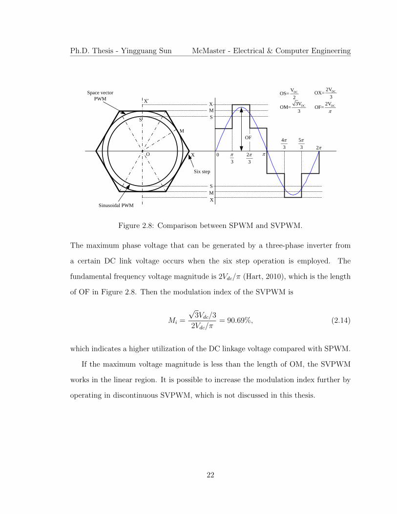
The maximum phase voltage that can be generated by a three-phase inverter from
a certain DC link voltage occurs when the six step operation is employed. The
fundamental frequency voltage magnitude is 2Vdc/π (Hart, 2010), which is the length
of OF in Figure 2.8. Then the modulation index of the SVPWM is
Mi =
√3Vdc/3
2Vdc/π= 90.69%, (2.14)
which indicates a higher utilization of the DC linkage voltage compared with SPWM.
If the maximum voltage magnitude is less than the length of OM, the SVPWM
works in the linear region. It is possible to increase the modulation index further by
operating in discontinuous SVPWM, which is not discussed in this thesis.
22

Ph.D. Thesis - Yingguang Sun McMaster - Electrical & Computer Engineering
2.4 Position Sensors and Interface
In (2.5), the transformation from α-β frame into d-q frame requires the knowledge of
rotor position θ. Moreover, the motor speed needs to be measured in the close loop
speed control. The speed and position acquisition is usually achieved by the position
sensors. Resolvers and Encoders are the two types of widely used position sensors in
industry.
2.4.1 Resolver and Its Interface
The working theory of the resolve is similar as a variable coupling transformer which
transmits the magnetic energy from the primary winding to the secondary winding.
It consists of two parts, the stator and the rotor. The typical resolver has a primary
winding on the rotor and two secondary windings on the stator (Szymczak et al.,
2014). However, this scheme requires slip rings for excitation of the magnetic field in
the rotor. So another type of resolver named variable reluctance resolver, which has
both the primary winding and secondary windings mounted on the resolver stator, is
more welcomed in industry. Figure 2.9 (a) depicts the variable reluctance resolvers
manufactured by Tamagawa (Tamagawa, 2014). In variable reluctance resolvers,
the sinusoidal variation caused by the rotor movement is coupled from the primary
winding to the secondary windings through the rotor saliency (Szymczak et al., 2014).
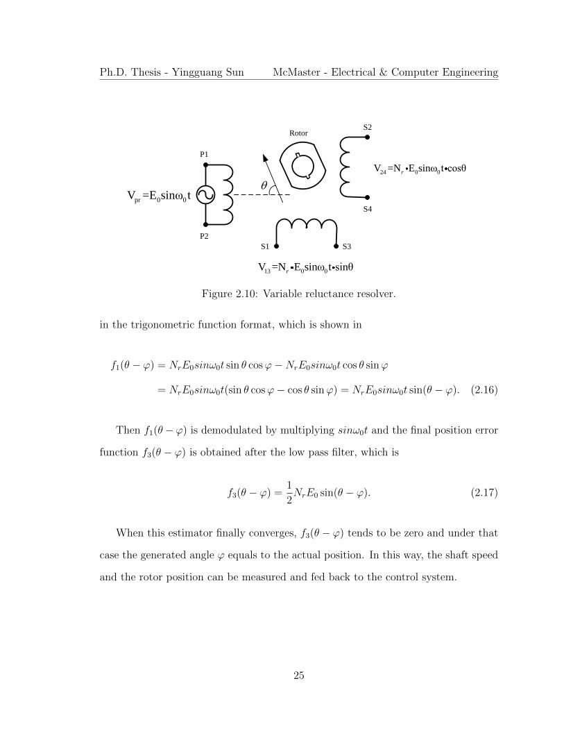
Figure 2.10 shows the structure of the variable reluctance resolver. The primary
winding is excited by sinusoidal voltages. The induced voltages in the secondary
windings are functions of the rotor position and their magnitudes are proportional to
the excitation voltage with a ratio Nr. Since the two secondary windings are displaced
orthogonal with each other, the induced voltages in the two windings have 90 phase
23

Ph.D. Thesis - Yingguang Sun McMaster - Electrical & Computer Engineering
(a) Tamagawa resolvers(b) Resolver interface evaluation
board (AD2S1200 Based)
Figure 2.9: Resolver and its interface.
shift. The voltage equations of the primary and secondary windings are shown in
Vpr = E0sinω0t
V13 = NrE0sinω0t sin θ (2.15)
V24 = NrE0sinω0t cos θ,
where E0 and ω0 denote the magnitude and frequency of the excitation voltage in the
primary winding.
From (2.15), it is clear to see that the rotor position θ is contained in the induced
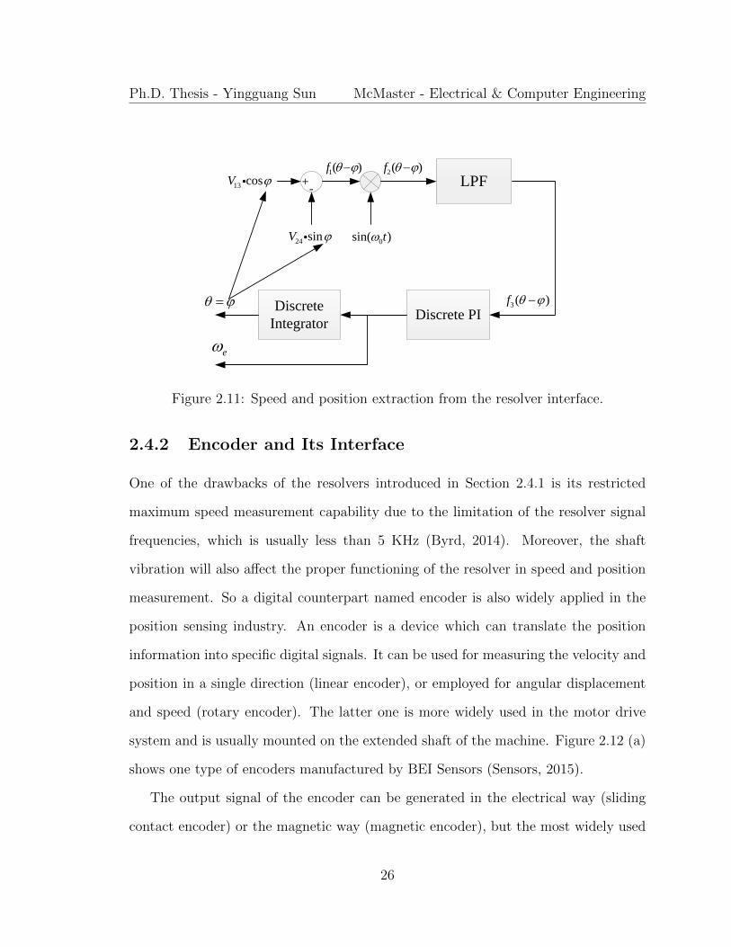
voltages V13 and V24. The extraction of the rotor position information and the exci-
tation of the primary winding both rely on the resolver interface. Figure 2.9 shows
one type of resolver interface, which is the evaluation board manufactured by Analog
Devices based on AD2S1200. The working theory of speed and position extraction
from the resolver interface is shown in Figure 2.11. In order to obtain the rotor po-
sition, an angle ϕ is generated by the interface and is incorporated with V13 and V24
24
Ph.D. Thesis - Yingguang Sun McMaster - Electrical & Computer Engineering
AC
Rotor
P1
P2
S2
S4
S3S1
pr 0 0V =E sinω t
24 0 0V =N E sinω t cosθr
13 0 0V =N E sinω t sinθr
Figure 2.10: Variable reluctance resolver.
in the trigonometric function format, which is shown in
f1(θ − ϕ) = NrE0sinω0t sin θ cosϕ−NrE0sinω0t cos θ sinϕ
= NrE0sinω0t(sin θ cosϕ− cos θ sinϕ) = NrE0sinω0t sin(θ − ϕ). (2.16)
Then f1(θ−ϕ) is demodulated by multiplying sinω0t and the final position error
function f3(θ − ϕ) is obtained after the low pass filter, which is
f3(θ − ϕ) =1
2NrE0 sin(θ − ϕ). (2.17)
When this estimator finally converges, f3(θ − ϕ) tends to be zero and under that
case the generated angle ϕ equals to the actual position. In this way, the shaft speed
and the rotor position can be measured and fed back to the control system.
25
Ph.D. Thesis - Yingguang Sun McMaster - Electrical & Computer Engineering
LPF
Discrete PIDiscrete
Integrator
0sin( )t
3( )f
e
+-
24 sinV
13 cosV 1( )f 2( )f
Figure 2.11: Speed and position extraction from the resolver interface.
2.4.2 Encoder and Its Interface
One of the drawbacks of the resolvers introduced in Section 2.4.1 is its restricted
maximum speed measurement capability due to the limitation of the resolver signal
frequencies, which is usually less than 5 KHz (Byrd, 2014). Moreover, the shaft
vibration will also affect the proper functioning of the resolver in speed and position
measurement. So a digital counterpart named encoder is also widely applied in the
position sensing industry. An encoder is a device which can translate the position
information into specific digital signals. It can be used for measuring the velocity and
position in a single direction (linear encoder), or employed for angular displacement
and speed (rotary encoder). The latter one is more widely used in the motor drive
system and is usually mounted on the extended shaft of the machine. Figure 2.12 (a)
shows one type of encoders manufactured by BEI Sensors (Sensors, 2015).
The output signal of the encoder can be generated in the electrical way (sliding
contact encoder) or the magnetic way (magnetic encoder), but the most widely used
26

Ph.D. Thesis - Yingguang Sun McMaster - Electrical & Computer Engineering
Figure 2.12: BEI incremental encoder.
encoder is the optical encoder. It has a specific pattern on the rotating disk which
can either allow or block the light passing through. A light source and a light sensor
need to work along with the rotating disk for producing position related disk counts.
In terms of the movement identification and interpretation of the output, the op-
tical encoder can be divided into the absolute encoder and the incremental encoder.
Figure 2.13 shows the different disk patterns of the absolute encoder and the incre-
mental encoder. They both have transparent windows which can pass through the
light on the opaque disk. In the absolute encoder, the position information can be
directly translated into specific binary codes as shown in Figure 2.13 (a). The Gray
code is also used in order to avoid the ambiguity in bit switching in absolute encoders
(Kimbrell, 2013).
Different with the absolute encoder, the incremental encoder shown in Figure 2.13
(b) only shows the relative position change and how far the shaft has rotated after
the encoder is powered up (Kimbrell, 2013). The pattern on the disk generates a
27

Ph.D. Thesis - Yingguang Sun McMaster - Electrical & Computer Engineering
011
010
001
000111
110
101
100
Transparent
Opaque
(a) Absolute encoder (b) Incremental encoder
Ref
Figure 2.13: Absolute and incremental encoders.
digital high voltage or low voltage based on the fact whether the light is allowed
to pass through the transparent window or is blocked by the opaque disk. The
generated electric pulse is counted for calculating the angular speed and position.
The electrical pulses can either be recorded in single channel or double channels
(quadrature output). In quadrature output, two different channels named A and
B are 90 phase shifted, which is shown in Figure 2.14. The two outputs can be
both high or low, which leads to four different states shown in Table. 2.2. The
quadrature output can provide four times pulses than the single channel. Besides
the two channels, certain incremental encoders also have a physical reference called
index reference which provides the zero position of the incremental encoder. When
the rotating disk passes through the reference, the position value will be reset to zero.
Table 2.2: Quadrature output states
States S1 S2 S3 S4Channel A 1 1 0 0Channel B 0 1 1 0
28

Ph.D. Thesis - Yingguang Sun McMaster - Electrical & Computer Engineering
A
B
Z
Position reset90
Figure 2.14: Quadrature output in incremental encoder.
Assuming that the incremental encoder can generate M pulses in one turn, the
current position θenc can be represented as
θenc =2πNcount
M, (2.18)
where the Ncount denotes the count of the electrical pulses.
The speed ωenc is calculated in
ωenc =2π∆Ncount
MTenc, (2.19)
where Tenc and ∆Ncount represent the sample time of the encoder and the number of
pulses between two consecutive encoder sample times.
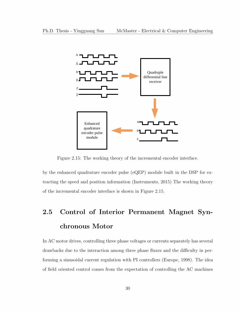
In order to cancel the common mode noises on the quadrature output during the
data transmission, the line drive signals with two separate wires for each channel
(A and A; B and B; Z and Z) are usually used. The line driver outputs are con-
verted to the common mode signal by specific quadruple differential line receivers,
e.g. AM26LV32C (Instruments, 2005). The converted encoder outputs are processed
29
Ph.D. Thesis - Yingguang Sun McMaster - Electrical & Computer Engineering
A
A
B
B
Z
Z
Quadruple
differential line
receiver
Enhanced
quadrature
encoder pulse
module
A
B
Z
Figure 2.15: The working theory of the incremental encoder interface.
by the enhanced quadrature encoder pulse (eQEP) module built in the DSP for ex-
tracting the speed and position information (Instruments, 2015) The working theory
of the incremental encoder interface is shown in Figure 2.15.
2.5 Control of Interior Permanent Magnet Syn-
chronous Motor
In AC motor drives, controlling three phase voltages or currents separately has several
drawbacks due to the interaction among three phase fluxes and the difficulty in per-
forming a sinusoidal current regulation with PI controllers (Europe, 1998). The idea
of field oriented control comes from the expectation of controlling the AC machines
30
Ph.D. Thesis - Yingguang Sun McMaster - Electrical & Computer Engineering
α-β
SVM
α-β abc
Trigger
signalsCurrent
controller
Current
controller
IPMSM
VSI
DC link
voltage
+_
+_
ref
qi
ref
di
du
qu u
u
di
qi i
i
abci
abcu
d-q
α-β d-q
Digital Signal
Processor
Torque
reference
Flux
reference
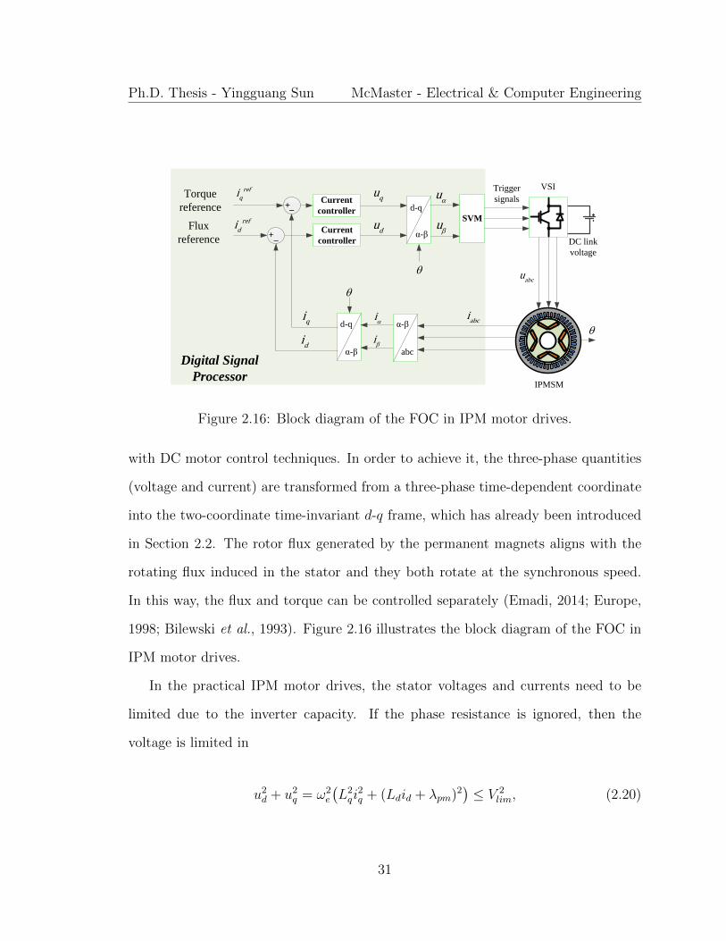
Figure 2.16: Block diagram of the FOC in IPM motor drives.
with DC motor control techniques. In order to achieve it, the three-phase quantities
(voltage and current) are transformed from a three-phase time-dependent coordinate
into the two-coordinate time-invariant d-q frame, which has already been introduced
in Section 2.2. The rotor flux generated by the permanent magnets aligns with the
rotating flux induced in the stator and they both rotate at the synchronous speed.
In this way, the flux and torque can be controlled separately (Emadi, 2014; Europe,
1998; Bilewski et al., 1993). Figure 2.16 illustrates the block diagram of the FOC in
IPM motor drives.
In the practical IPM motor drives, the stator voltages and currents need to be
limited due to the inverter capacity. If the phase resistance is ignored, then the
voltage is limited in
u2d + u2q = ω2e
(L2qi
2q + (Ldid + λpm)2
)≤ V 2
lim, (2.20)
31

Ph.D. Thesis - Yingguang Sun McMaster - Electrical & Computer Engineering
Current limit cycle
Maximum torque-per-
ampere trajectory
Voltage limit ellipses
di
qi
1e 2e
Voltage limited maximum
output trajectory
1P
2P
3P
O
I
IIIII
O
eT
e1 2
(a) Voltage constraints, current constraints, MTPA and
votlage limited maximum output trajectory (b) Torque-speed curve
Figure 2.17: Optimal IPM motor operation with voltage and current limits andtorque-speed curve.
where Vlim denotes the maximum output voltage of the three phase inverter (Mori-
moto et al., 1990; Cheng and Tesch, 2010), which is 2Vdc/π mentioned in Section 2.3.
The voltage limit is represented as the voltage limit ellipse shown in Figure 2.17 (a).
The stator current also has the limitation decided by the continuous stator current
rating of the machine and the output current limit of the inverter (Morimoto et al.,
1990). The current limit Ilim is illustrated in
i2d + i2q ≤ I2lim, (2.21)
which is depicted as a current limit cycle shown in Figure 2.17 (a).
Assume θs is the angle between the stator current vector Is and the negative
direction of d axis, the relationship between the stator current and the d-q axes
32

Ph.D. Thesis - Yingguang Sun McMaster - Electrical & Computer Engineering
currents are shown in
id = −Is cos θs
iq = Is sin θs. (2.22)
Then the electromagnetic torque shown in (2.8) can be represented as a function of Is
and θs. In order to get the maximum utilization of the current, the maximum torque-
per-ampere (MTPA) needs to achieved. For a specific Is, the maximum torque can
be obtained when dTe/dθs = 0. Combining (2.8) and (2.22), the following equation
is obtained as
2(Lq − Ld)Is cos2 θs + λpm cos θs − (Lq − Ld)Is = 0. (2.23)
Combining (2.22) and (2.23), the final relationship between id and iq to achieve
MTPA is shown in
id =λpm −
√λ2pm + 4(Lq − Ld)2i2q2(Lq − Ld)
. (2.24)
The MTPA trajectory is shown in Figure 2.17 (a). Before the MTPA trajectory
intersects the current limit cycle, the rated torque can be maintained by applying
the current vector fixed in P1 and the motor speed can increase with the maximum
torque until it reaches the motor base speed ω1 (Morimoto et al., 1990), which is
ω1 =Vlim√
L2qi
2q + (Ldid + λpm)2
. (2.25)
33

Ph.D. Thesis - Yingguang Sun McMaster - Electrical & Computer Engineering
When the motor speed is below the base speed, the motor is running in region I
in Figure 2.17 (b), which is usually called the constant torque mode. If the motor
speed keeps increasing, the current vector trajectory has to move along the current
limit cycle towards P2, which is the intersection of the current limit cycle and the
voltage limited maximum output trajectory (Morimoto et al., 1990; Uddin et al.,
2002). When the current vector trajectory moves from P1 to P2, the motor speed
increases from ω1 to ω2 and the currents in d-q axes need to satisfy
id =−λpm +
√V 2lim
ω2e− L2
qi2q
Ld
i2d + i2q = I2lim. (2.26)
The above operation condition is also represented as region II in the torque-speed
curve in Figure 2.17 (b). This region consists of all the intersections of the current
limit cycle and voltage limit ellipses. As shown in (2.26), the current and voltage both
reach to the limits and this region is usually named constant power region. When
the motor speed is above ω2, the Vlim is satisfied while the current limit Ilim can not
be reached. It is called reduced power mode (Bianchi and Bolognani, 1997) and is
depicted as the trajectory from P2 to P3 in Figure 2.17 (a) and the region III in
Figure 2.17 (b).
2.6 Conclusions
In this chapter, the basic working theories of the components used in the modern elec-
tric motor drive system are introduced. In order to generate electromagnetic torque
34

Ph.D. Thesis - Yingguang Sun McMaster - Electrical & Computer Engineering
for propelling the mechanical load, the DC voltage needs to be converted to three
phase AC voltages through the voltage source inverter. By using SPWM or SVPWM
illustrated in this chapter, this conversion can be achieved. The electromagnetic
torque is generated by the interaction between the rotating stator flux and the rotor
flux provided by the permanent magnets. The electromagnetic torque is controlled
by regulating the currents in the rotor reference frame. The field oriented control and
IPMSM optimal operation are introduced and explained in this chapter. Moreover, in
order to achieve field oriented control, the knowledge of the rotor position and speed
is needed. The working theories of the position sensors and their interfaces are also
explained in this chapter in detail.
35

Chapter 3
Existing Sensorless Control
Methods of IPM Motor Drives
3.1 Introduction
High performance AC motor control requires the knowledge of rotor position and
speed. Specific position sensors (resolver and encoder) are normally used in pro-
viding the position and speed information in real time as introduced in Section 2.4.
However, the existence of the position sensor increases the machine size and frequent
maintenance of the sensors is needed. Moreover, additional signal conditioning cir-
cuits are needed for interfacing the sensor output signals with the digital controller,
which increase the cost of the entire drive system. Additionally, the transmission
between the sensors and the controller through specific interfaces may be affected by
the external noise that degrades the system robustness. Hence, much efforts have
been focused on new methods for speed and position sensorless control of IPMSM
drives to avoid sensor-related issues (Sun et al., 2015). In this chapter, the speed
36

Ph.D. Thesis - Yingguang Sun McMaster - Electrical & Computer Engineering
and position estimation algorithms of IPMSM drives at standstill, low speed, high
speed and wide speed range are introduced respectively. Typical existing methods
are explained explicitly and are implemented experimentally as benchmark references
of the proposed methods.
3.2 EMF Based Speed and Position Estimation
Sensorless control methods can be classified into two categories. The first category is
the electromotive force (EMF) based estimation methods relying on the measurement
of the stator voltages and currents for medium and high speed operations (Morimoto
et al., 2002; Chen et al., 2003; Nahid-Mobarakeh et al., 2007; Genduso et al., 2010; Liu
and Zhu, 2014a; Shinnaka, 2006; Chan et al., 2008; Hasegawa and Matsui, 2009; Chi
et al., 2009; Zhao et al., 2013; Wang et al., 2013b, 2014; Zhao et al., 2015a,b; Bolognani
et al., 1999; Kim and Kook, 1999; Boussak, 2005). The most straightforward way of
obtaining the position information is to calculate the EMF or flux in open loop or
simply estimating flux by integrating the EMF. However, the integration degrades
due to the drift problem and is sensitive to machine phase resistance. In order to
improve position estimation, the Back-EMF, extended EMF and flux were estimated
by state observers (Morimoto et al., 2002; Chen et al., 2003; Nahid-Mobarakeh et al.,
2007; Genduso et al., 2010; Liu and Zhu, 2014a; Shinnaka, 2006; Chan et al., 2008;
Hasegawa and Matsui, 2009), sliding mode observers (Chi et al., 2009; Zhao et al.,
2013; Wang et al., 2013b, 2014; Zhao et al., 2015a,b) and extended Kalman Filters
(Bolognani et al., 1999; Kim and Kook, 1999; Boussak, 2005). In this section, the
method employing extend EMFs in the estimated rotor reference frame (Morimoto
et al., 2002) is introduced in detail.
37

Ph.D. Thesis - Yingguang Sun McMaster - Electrical & Computer Engineering
d
q
e
ˆe
Figure 3.1: Different reference frames in IPMSM drives.
In sensorless field oriented control of permanent magnet motor drives, three ref-
erence frames shown in Figure 3.1 are normally utilized. The voltages and currents
in the stationary reference frame (α-β frame) can be transformed to the rotor refer-
ence frame (d-q frame) or the estimated rotor reference frame (δ-γ frame) by actual
position θ or estimated position θ.
The fundamental frequency voltage equations of IPM motor in d-q frame are shown
in
[ud
uq
]=
[Rs −ωeLqωeLd Rs
][id
iq
]+
[Ld 0
0 Lq
]p
[id
iq
]+ ωeλpm
[0
1
]. (3.1)
In EMF based methods, the rotor position can be obtained from the EMF or
flux linkage due to the permanent magnets by using different kinds of observers.
Particularly, the extended EMFs in δ-γ frame are utilized to extract the rotor position
and speed at medium and high speed conditions (Morimoto et al., 2002). If the square
38
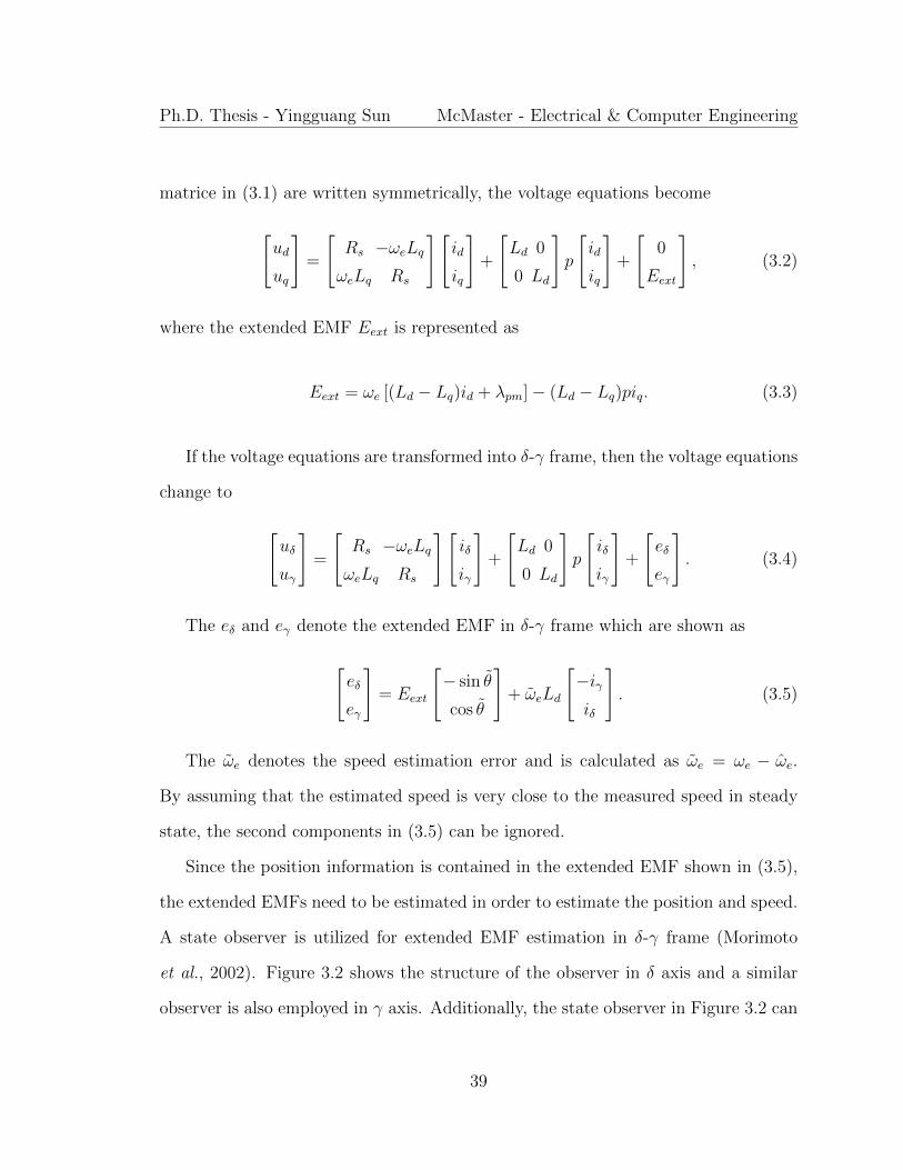
Ph.D. Thesis - Yingguang Sun McMaster - Electrical & Computer Engineering
matrice in (3.1) are written symmetrically, the voltage equations become
[ud
uq
]=
[Rs −ωeLqωeLq Rs
][id
iq
]+
[Ld 0
0 Ld
]p
[id
iq
]+
[0
Eext
], (3.2)
where the extended EMF Eext is represented as
Eext = ωe [(Ld − Lq)id + λpm]− (Ld − Lq)piq. (3.3)
If the voltage equations are transformed into δ-γ frame, then the voltage equations
change to
[uδ
uγ
]=
[Rs −ωeLqωeLq Rs
][iδ
iγ
]+
[Ld 0
0 Ld
]p
[iδ
iγ
]+
[eδ
eγ
]. (3.4)
The eδ and eγ denote the extended EMF in δ-γ frame which are shown as
[eδ
eγ
]= Eext
[− sin θ
cos θ
]+ ωeLd
[−iγiδ
]. (3.5)
The ωe denotes the speed estimation error and is calculated as ωe = ωe − ωe.
By assuming that the estimated speed is very close to the measured speed in steady
state, the second components in (3.5) can be ignored.
Since the position information is contained in the extended EMF shown in (3.5),
the extended EMFs need to be estimated in order to estimate the position and speed.
A state observer is utilized for extended EMF estimation in δ-γ frame (Morimoto
et al., 2002). Figure 3.2 shows the structure of the observer in δ axis and a similar
observer is also employed in γ axis. Additionally, the state observer in Figure 3.2 can
39
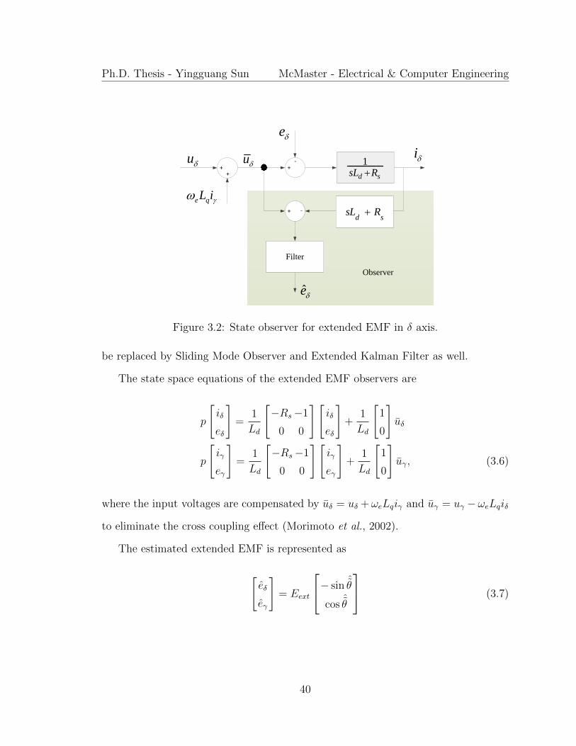
Ph.D. Thesis - Yingguang Sun McMaster - Electrical & Computer Engineering
1
d ssL R+
+
u
e qL i
u +-
e
i
+ -d s
sL R
Filter
e
Observer
Figure 3.2: State observer for extended EMF in δ axis.
be replaced by Sliding Mode Observer and Extended Kalman Filter as well.
The state space equations of the extended EMF observers are
p
[iδ
eδ
]=
1
Ld
[−Rs−1
0 0
][iδ
eδ
]+
1
Ld
[1
0
]uδ
p
[iγ
eγ
]=
1
Ld
[−Rs−1
0 0
][iγ
eγ
]+
1
Ld
[1
0
]uγ, (3.6)
where the input voltages are compensated by uδ = uδ + ωeLqiγ and uγ = uγ − ωeLqiδ
to eliminate the cross coupling effect (Morimoto et al., 2002).
The estimated extended EMF is represented as
[eδ
eγ
]= Eext
− sin ˆθ
cos ˆθ
(3.7)
40

Ph.D. Thesis - Yingguang Sun McMaster - Electrical & Computer Engineering
and the estimated position estimation error is calculated as
ˆθ = arctan
(− eδeγ
). (3.8)
The estimated position error can be processed with a Phase Locked Loop (PLL)
which consists of a PI regulator and an integrator for speed and position estimation.
The block diagram of the PLL is shown in Figure 3.3. The estimated speed is obtained
directly from the PLL output. Assuming that the ˆθ = θ − θ, the close loop transfer
function of the PLL from the actual position to the estimated one is represented in
θ
θ=
Kps+Ki
s2 +Kps+Ki
, (3.9)
where Kp and Ki denote the proportional gain and the integral gain in the PI reg-
ulator. The PLL contains two integrations and the steady state error is zero with
a ramp input (Dorf and Bishop, 2010). The Kp and Ki can be designed based on
the PLL bandwidth requirements, but the theoretical numbers need to be adjusted
heuristically by balancing the estimation bandwidth and noise attenuation (Morimoto
et al., 2002; Jeong et al., 2005; Jang et al., 2004; Al-nabi et al., 2013).
Since the EMF components are proportional to the motor speed, the extraction
of EMF is challenging at low speed condition. Moreover, the voltage drop due to the
stator resistance and inverter nonlinearities also affect estimation performance of the
EMF based methods at low speed.
41

Ph.D. Thesis - Yingguang Sun McMaster - Electrical & Computer Engineering
PI
e
e ˆ
1
s
ˆe
Error
Calculation
PLL
arctan
Figure 3.3: Extended EMF based position estimator.
3.3 Saliency Tracking Based Speed and Position
Estimation
In order to achieve speed and position estimation at low speed, the saliency tracking
based methods, which usually employ high frequency signal injection into different
frames of the machine (Kim et al., 2004; Jeong et al., 2005; Bolognani et al., 2011;
Kim et al., 2012; Aihara et al., 1999; Jang et al., 2004; Foo et al., 2010; Gong and
Zhu, 2013; Zaim et al., 2014; Huang et al., 2014; Yang, 2015; Noguchi et al., 1998; Liu
and Zhu, 2014b), are also widely utilized. These methods exploited the anisotropic
property of IPM machines caused by spatial saliency or magnetic saturation. In (Kim
et al., 2004; Jeong et al., 2005; Bolognani et al., 2011; Kim et al., 2012), rotating sinu-
soidal voltage signals were injected into stationary reference frame and the resulting
carrier frequency currents were demodulated for extracting the rotor position infor-
mation. Another major type of injection method is called pulsating voltage injection
42

Ph.D. Thesis - Yingguang Sun McMaster - Electrical & Computer Engineering
method (Aihara et al., 1999; Jang et al., 2004; Foo et al., 2010; Gong and Zhu, 2013).
This method relied on injecting sinusoidal voltage signals into δ or γ axis and the
induced currents in γ or δ axis was utilized for position estimation. Compared with
rotating sinusoidal injection, the pulsating voltage injection has the benefits of simpler
demodulation procedures and less torque ripples. Other injection types like square
wave voltage injection (Zaim et al., 2014; Huang et al., 2014; Yang, 2015), sinusoidal
current injection (Noguchi et al., 1998) and pulsating voltage injection into stationary
reference frame (Liu and Zhu, 2014b) were also applied for position sensing. Besides
signal injection, methods relying on high frequency excitation by PWM switching
(Schroedl, 1996; Petrovic et al., 2003) were also employed for sensorless control of
permanent magnet motor drives.
In this section, the pulsating sinusoidal voltage injection based method (Zhu and
Gong, 2011; Gong and Zhu, 2013) is introduced as an example of the saliency tracking
based methods. In signal injection based method, since the injection frequency is
usually much higher than the fundamental frequency and the machine speed is low, the
resistive voltage drop and EMF components can be ignored in the voltage equations.
The high frequency voltage equations are rewritten as
[udh
uqh
]=
[Ld 0
0 Lq
]p
[idh
iqh
], (3.10)
where udqh and idqh represent the d-q frame voltages and currents in the injection
frequency.
43

Ph.D. Thesis - Yingguang Sun McMaster - Electrical & Computer Engineering
The transformation from δ-γ frame to d-q frame is shown as
T (θ) =
[cos(θ) sin(θ)
− sin(θ) cos(θ)
], (3.11)
where the position error θ can be represented as θ = θ − θ.
The voltage equations in δ-γ frame can be obtained from (3.10) and (3.11), which
is
[uδh
uγh
]= T−1(θ)
[Ld 0
0 Lq
]T (θ)p
[iδh
iγh
]. (3.12)
The above equations are further developed as
p
iδhiγh
=
1Lm
+ 1Ln
cos(2θ) 1Ln
sin(2θ)
1Ln
sin(2θ) 1Lm− 1
Lncos(2θ)
uδhuγh
, (3.13)
where Lm = 2LdLq/(Ld + Lq) and Ln = 2LdLq/(Lq − Ld).
In the proposed method, the high frequency voltage is injected in δ axis. The
injected voltages are mathematically represented as
[uδh
uγh
]= Vh
[cos(ωht)
0
], (3.14)
where Vh and ωh represent the magnitude and frequency of the injected voltage.
Combining (3.13) and (3.14), the resulting currents in the injection frequency are
44

Ph.D. Thesis - Yingguang Sun McMaster - Electrical & Computer Engineering
developed as
[iδh
iγh
]=
[I1 + I2 cos(2θ)
I2 sin(2θ)
]sin(ωht), (3.15)
where I1 = Vh/(ωhLm) and I2 = Vh/(ωhLn).
From (3.15), it is easy to see that the position information θ is contained both in
iδh and iγh. In order to obtain the position information, a demodulation method con-
taining a band-pass filter (BPF) and a low-pass filter (LPF) is utilized for processing
the resulting current in γ axis, as shown in Figure 3.4. First of all, the BPF is used
for extracting iγh from iγ. Then the multiplication of sin(ωht) is applied to the output
of the BPF. Finally, a LPF is used to eliminate the high frequency components in the
obtained signal. A function containing the position error is extracted at the output
of the LPF, which is represented as
f(θ) =1
2I2 sin(2θ). (3.16)
Similar to the extended EMF based method, a PLL is also used for estimating
the speed and position in the demodulation based position estimator. When θ is
small enough, sin(2θ) ≈ 2θ. So f(θ) can be applied as the input of the PLL and the
outputs are the estimated speed and position.
The saliency tracking based methods are parameter independent and suitable for
low speed operations including standstill conditions. However, larger torque ripples
and extra losses are introduced in these methods due to the superimposition of extra
signals on the fundamental frequency components. Additionally, the control band-
width is limited due to demodulation of the carrier frequency current components in
45
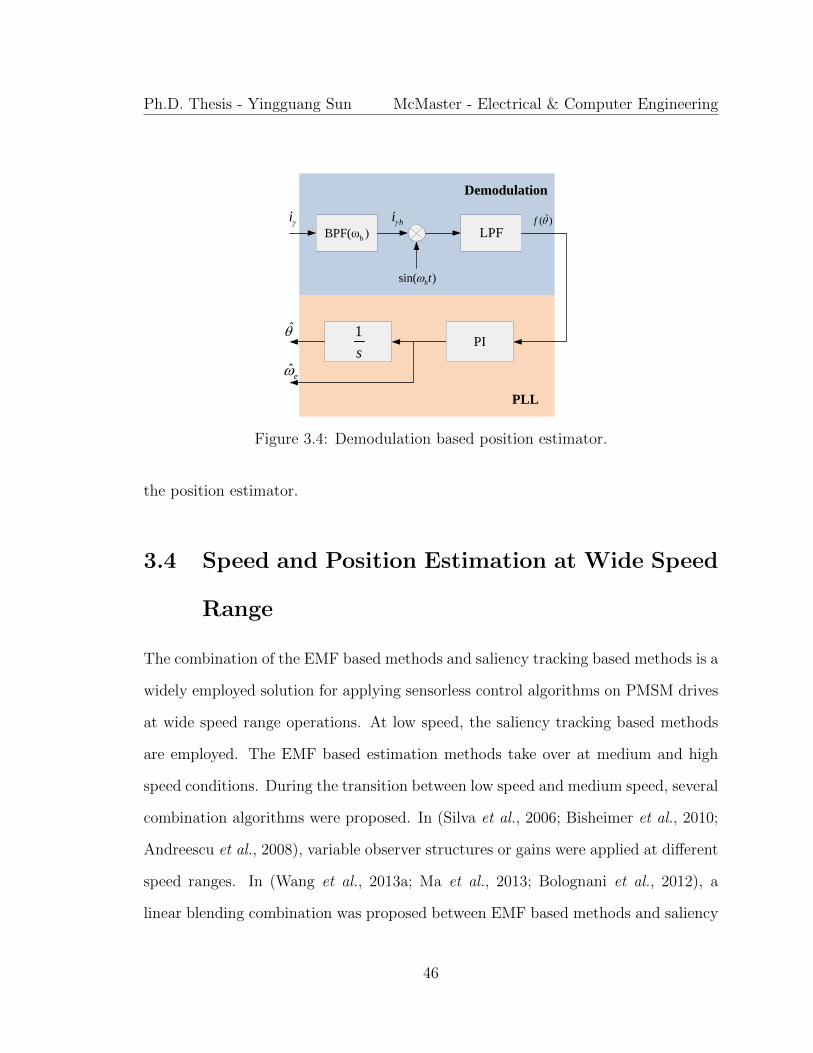
Ph.D. Thesis - Yingguang Sun McMaster - Electrical & Computer Engineering
LPF
PI
ihBPF(ω )
hi
sin( )ht
( )f
1
s
ˆe
Demodulation
PLL
Figure 3.4: Demodulation based position estimator.
the position estimator.
3.4 Speed and Position Estimation at Wide Speed
Range
The combination of the EMF based methods and saliency tracking based methods is a
widely employed solution for applying sensorless control algorithms on PMSM drives
at wide speed range operations. At low speed, the saliency tracking based methods
are employed. The EMF based estimation methods take over at medium and high
speed conditions. During the transition between low speed and medium speed, several
combination algorithms were proposed. In (Silva et al., 2006; Bisheimer et al., 2010;
Andreescu et al., 2008), variable observer structures or gains were applied at different
speed ranges. In (Wang et al., 2013a; Ma et al., 2013; Bolognani et al., 2012), a
linear blending combination was proposed between EMF based methods and saliency
46

Ph.D. Thesis - Yingguang Sun McMaster - Electrical & Computer Engineering
tracking based methods during the switching process, which is shown in this section.
As shown in Figure 3.5, two speed boundaries are selected as N1 and N2. If the
machine speed is lower than N1, only the estimated speed and position from the
pulsating voltage injection method are used. If the machine speed is higher than
N2, only the estimated speed and position from the extended EMF based method
are employed. If the motor speed is between N1 and N2 , then the final estimated
speed and position are the linear combinations of speeds and positions estimated by
both methods. The relationship is shown in (3.17) and (3.18), where N denotes the
estimated speed in rpm.
θ =
θlow
∣∣∣N ∣∣∣ ≤ N1
θhigh
∣∣∣N ∣∣∣ ≥ N2
N2−|N|N2−N1
θlow +|N|−N1
N2−N1θhigh N1 <
∣∣∣N ∣∣∣ < N2
(3.17)
ω =
ωlow
∣∣∣N ∣∣∣ ≤ N1
ωhigh
∣∣∣N ∣∣∣ ≥ N2
N2−|N|N2−N1
ωlow +|N|−N1
N2−N1ωhigh N1 <
∣∣∣N ∣∣∣ < N2
(3.18)
The block diagram of the combined sensorless control system is shown in Figure
3.6. Two position estimators and two PLLs are needed in the combined system, which
increases the system complexity. This combined algorithm was implemented in the
experimental test bench as a benchmark reference for the proposed unified method.
47
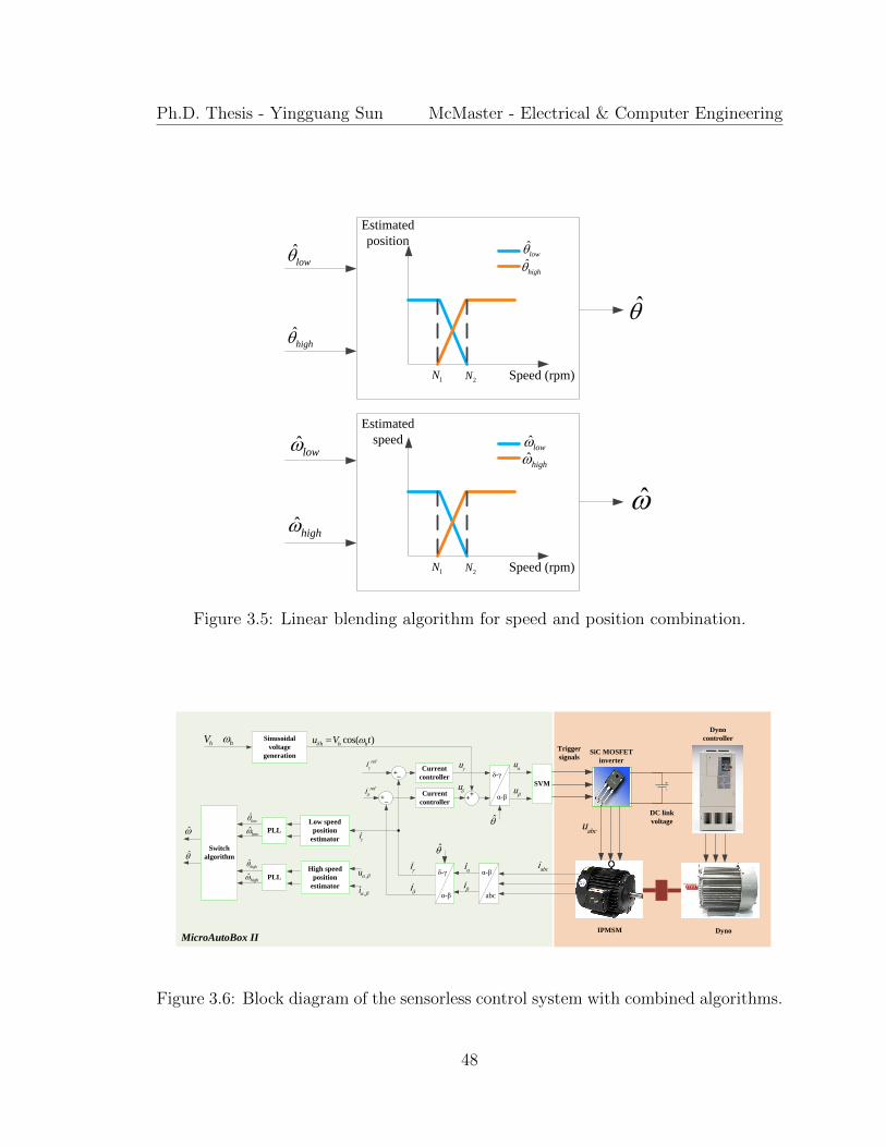
Ph.D. Thesis - Yingguang Sun McMaster - Electrical & Computer Engineering
ˆlow
Speed (rpm)
Estimated
position ˆlow
1N2N
ˆhigh
ˆhigh
ˆlow
Speed (rpm)
Estimated
speed ˆlow
1N2N
ˆhigh
ˆhigh
Figure 3.5: Linear blending algorithm for speed and position combination.
Trigger
signals
IPMSM
SiC MOSFET
inverter
DC link
voltage
abcu
Dyno
Dyno
controller
α-β
SVM
α-β abc
Current
controller
Current
controller
+_
+_
refi
refi
u
u
u
u
i
i
i
i
abci
δ-γ
α-β δ-γ
Low speed
position
estimator
High speed
position
estimator
ˆlow
,u
,i
Switch
algorithm
i
MicroAutoBox II
Sinusoidal
voltage
generation
hhV cos( )h h hu V t
++
PLL
PLL
ˆlow
ˆhigh
ˆhigh
Figure 3.6: Block diagram of the sensorless control system with combined algorithms.
48

Ph.D. Thesis - Yingguang Sun McMaster - Electrical & Computer Engineering
3.5 Initial Position Estimation
The function of position error shown in (3.16) implies that only 2θ is available for
the low speed position estimator. So the estimated position will have an ambiguity
of 180, which implies that the initial position and the magnetic polarity need to be
identified at the machine startup. According to the literature, the existing starting
procedures can be classified into three categories: (1). Physical alignment of the rotor
magnetic axis (d axis) in the direction of a fixed stator magnetic field generated by
a DC current excitation; (2). Starting the rotor with a rotating stator magnetic field
in open loop; (3). Detection of stator inductance variations by different estimation
algorithms (Tursini et al., 2003; Antonello et al., 2015).
The first procedure can be achieved by simply imposing a constant voltage vector
to the inverter to align d axis to a specific phase direction. However, the application
of this method is restricted by the presence of load torque and the availability of
movement of the mechanical system. The second procedure aims at rotating the
machine in open loop with specific rotating magnetic field until the machine back-
emf (proportional to the machine speed) is sufficiently large for position estimation.
Nevertheless, only limited torque is allowed at startup if this procedure is employed
(Tursini et al., 2003; Chen et al., 2003; Genduso et al., 2010; Antonello et al., 2015).
The existing initial position estimation algorithms are mostly concentrating on
estimating the rotor position by identifying the location of the minimum stator in-
ductance. Besides the continuous signal injection introduced in Section 3.2, the pulse
voltage injection based methods (Antonello et al., 2015; Schroedl, 1996; Nakashima
et al., 2000; Tursini et al., 2003; Khlaief et al., 2012) were also employed for initial
position estimation.
49

Ph.D. Thesis - Yingguang Sun McMaster - Electrical & Computer Engineering
3.5.1 Short Pulse Voltage Injection for Initial Position Esti-
mation
Different with the continuous injection, pulse voltage signals can be utilized for iden-
tifying the initial position as well. The basic idea of these methods is searching for
the minimum inductance location by measuring the peak current responses due to
the injected short pulse voltage vectors applied along different directions with respect
to the stator (Antonello et al., 2015). The higher di/dt indicates a smaller induc-
tance along that direction. In (Nakashima et al., 2000), twenty-one voltage vectors
were applied in different directions along the stator in order to find the minimum
inductance location which indicates the orientation of d axis. In (Schroedl, 1996;
Tursini et al., 2003; Khlaief et al., 2012), three voltage vectors were injected among
three phases and the induced peak phase current responses were recorded for position
estimation. The mathematical function arctan is applied for calculating the position
in (Schroedl, 1996) and a complicated table was used in (Khlaief et al., 2012) to
calculate the position by using arctan(θ) ≈ θ approximately.
In (Boussak, 2005; Khlaief et al., 2012), voltage pulses were injected in phase A, B
and C respectively by applying gate signals V(100), V(010) and V(001) to the voltage
source inverter directly and the current peaks were recorded for position estimation.
The injection scheme is shown in Figure 3.7.
50
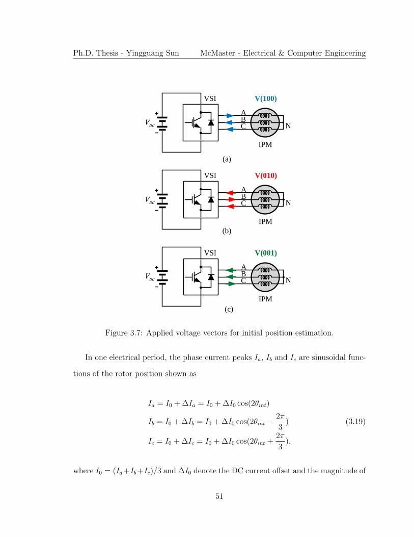
Ph.D. Thesis - Yingguang Sun McMaster - Electrical & Computer Engineering
ABC
IPM
NDCV
V(100)VSI
ABC
IPM
N
V(010)VSI
ABC
IPM
N
V(001)VSI
(a)
(b)
(c)
DCV
DCV
Figure 3.7: Applied voltage vectors for initial position estimation.
In one electrical period, the phase current peaks Ia, Ib and Ic are sinusoidal func-
tions of the rotor position shown as
Ia = I0 + ∆Ia = I0 + ∆I0 cos(2θint)
Ib = I0 + ∆Ib = I0 + ∆I0 cos(2θint −2π
3) (3.19)
Ic = I0 + ∆Ic = I0 + ∆I0 cos(2θint +2π
3),
where I0 = (Ia+Ib+Ic)/3 and ∆I0 denote the DC current offset and the magnitude of
51

Ph.D. Thesis - Yingguang Sun McMaster - Electrical & Computer Engineering
Table 3.1: Initial Position Estimation
Sign (∆Ia) Sign (∆Ib) Sign (∆Ic) Estimated initial position θint+ - - ∈ [−1515] or ∈ [165195]+ + - ∈ [1545] or ∈ [195225]- + - ∈ [4575] or ∈ [225255]- + + ∈ [75105] or ∈ [255285]- - + ∈ [105135] or ∈ [285315]+ - + ∈ [135165] or ∈ [315345]
the fluctuated components. The current differences ∆Ia, ∆Ib and ∆Ic are calculated
as ∆Ia = Ia − I0, ∆Ib = Ib − I0 and ∆Ic = Ic − I0 respectively. Based on (3.19), the
relationship among phase current differences is shown in
tan 2θint =
√3(∆Ib −∆Ic)
2∆Ia −∆Ib −∆Ic. (3.20)
The initial rotor position is then calculated as
θint =1
2arctan(
√3(∆Ib −∆Ic)
2∆Ia −∆Ib −∆Ic). (3.21)
The range of arctan(2θint) is between [−90 90], then the detected initial position
θint is within [−45 45], which leads to an ambiguity of 90 electrical degree in the
estimation results. In order to solve this problem, Table 3.1 was also used for identify
the initial position.
With (3.21) and Table 3.1, the estimated initial position still contains an ambiguity
of 180 as in the sinusoidal injection based method. This ambiguity can be eliminated
by utilizing magnetic polarity detection, which is going to be introduced in Section
3.5.2.
52

Ph.D. Thesis - Yingguang Sun McMaster - Electrical & Computer Engineering
3.5.2 Magnetic Polarity Detection
The spatial saliency of the IPM machine performs two periods in one electric cycle.
The position estimation results contain an ambiguity of 180, which leads to the re-
verse rotation of the machine shaft. In order to detect the magnetic polarity, several
methods have been proposed in the literature (Kim et al., 2004; Jeong et al., 2005;
Kondo et al., 1995; Aihara et al., 1999; Khlaief et al., 2012; Noguchi et al., 1998;
Murakami et al., 2012; Gong and Zhu, 2013). In (Kim et al., 2004; Jeong et al.,
2005), the second order components of the induced high frequency currents were de-
modulated for polarity detection. The robustness of the secondary harmonic based
method is limited due to the small magnitude of the second order components. In
(Kondo et al., 1995; Aihara et al., 1999; Khlaief et al., 2012; Noguchi et al., 1998;
Murakami et al., 2012; Gong and Zhu, 2013), the magnetic saturation of the stator
core was used for determining the location of the north magnetic pole. The decrease
of d axis inductance can be reflected in the increase of current response, both in d-q
inductances and phase inductances (Kondo et al., 1995; Aihara et al., 1999; Khlaief
et al., 2012). The voltage reference oscillations of the current controller due to satu-
ration were observed for polarity detection in (Noguchi et al., 1998) and the magnetic
hysteresis phenomenon was utilized for identifying magnetic north pole in (Murakami
et al., 2012). Both methods were not straightforward for real time implementation.
In (Gong and Zhu, 2013), the saturation based polarity detection algorithm was ap-
plied in the running state as well as standstill conditions while the detection time was
relatively long. In these methods, the need for magnetic saturation of the stator iron
may lead to a high current for polarity detection in some machines, which requires
inverters with higher power rating to ensure robust detection of magnetic polarity.
53

Ph.D. Thesis - Yingguang Sun McMaster - Electrical & Computer Engineering
In this chapter, the dual voltage injection based polarity detection method (Gong
and Zhu, 2013; Kondo et al., 1995; Aihara et al., 1999) is introduced in detail. In
this method, dual voltage pulses were injected in estimated d axis after the location
of the magnetic axis had been estimated. The pulse aligned with the north magnetic
pole increases the magnetization of the stator core and leads to a smaller Ld. The
other voltage pulse aligned with the south pole decreases the magnetization of the
stator core and results in a larger Ld. As shown in Figure 3.8, if a pair of dual voltage
pulses with the same magnitude and inverse directions (V pospul = V neg
pul ) is injected in
estimated d axis, the difference between peak current values of the resulting currents
can be employed for determining the magnetic polarity. The direction of the voltage
pulse with higher current response indicates the direction of the magnetic north pole
(Gong and Zhu, 2013). In Figure 3.8, if the positive direction of the estimated d axis
aligns with the north magnetic pole, Ipospeak should be larger than Inegpeak. Otherwise the
positive direction of the estimated d axis aligns with the south magnetic pole and the
compensation of 180 is needed. The framework of the dual voltage injection based
polarity detection method is illustrated in Figure 3.9. Since this inductance variation
is also reflected in the phase inductances, the magnetic polarity can be detected by
observing the phase currents as well (Boussak, 2005; Khlaief et al., 2012).
3.6 Conclusions
This chapter reviews the existing speed and position estimation algorithms at stand-
still, low speed and high speed conditions. The pulsating voltage injection based
method, the extended EMF based method and their combination are explained in
detail at running state. Those above mentioned methods were implemented in the
54

Ph.D. Thesis - Yingguang Sun McMaster - Electrical & Computer Engineering
-10 -5 0 5 10
0.2
0.25
0.3
0.35
0.4
0.45
id (A)
d
(Wb
)
-12 12
pos
pulV
neg
pulVneg
peakI
pos
peakI
pos neg
peak peakI I
( , 0)d di
Figure 3.8: Dual voltage injection based method for magnetic polarity detection.
Dual voltage pulse
injection
Record the
current peaks
ˆ ˆ 0 ˆ ˆ 180
Y
N>
Calculate andpos
peakI neg
peakI
pos
peakI neg
peakI
Figure 3.9: Framework of the dual voltage pulse injection based method
55

Ph.D. Thesis - Yingguang Sun McMaster - Electrical & Computer Engineering
prototype IPMSM drive system as benchmark reference of the proposed optimization
based sensorless algorithms. For initial position estimation, both the sinusoidal in-
jection and short pulse injection can be utilized. Since the machine saliency performs
two periods in one electrical cycle, the magnetic polarity detection is indispensable
for obtaining the positive direction of the magnetic axis. The existing short pulse
injection based initial position estimation methods and polarity detection methods
have been introduced in this chapter. The detailed comparisons between the existing
methods and the proposed methods will be presented in Chapter 7.
56

Chapter 4
Novel Nonlinear IPM Motor Model
4.1 Introduction
Machine models are instrumental in the analysis of the performance and tuning of
the parameters of position estimation algorithms prior to actual experimental vali-
dation. The typical machine model assumes constant parameters and is widely used
for such purposes. However, this machine model is not suitable for position estima-
tion especially for polarity detection, because of their inaccuracies and their inability
to model nonlinearities, which are caused by the saturation and cross-saturation ef-
fects. Therefore, Look-up tables (LUTs) relating current to inductance or flux linkage
are commonly employed for nonlinear machine modeling. The look-up tables of the
prototype IPM machine were measured experimentally with typical motor drive com-
ponents. However, the use of the derivative of flux in the machine dynamics often
gives rise to oscillations and can reduce the accuracy of the transient response, when
using those look-up tables. Therefore, an improved method for implementing the
nonlinear machine model is introduced in this chapter and is used for investigating
57

Ph.D. Thesis - Yingguang Sun McMaster - Electrical & Computer Engineering
Table 4.1: Parameters of Prototype IPM Motor Drives
Parameter Value
Rated power Pr 5 KW
Rated speed Nr 1800 rpm
Number of pole pairs P 5
Rated voltage (L-L) Vr 460 V
Rated current Ir 9.4 A
Rated torque Tr 29.7 Nm
d axis inductance Ld 10.5 mH
q axis inductance Lq 12.9 mH
Stator resistance Rs 400 mΩ
PM flux λpm 343.05 mWb
Shaft friction B 1.3× 10⁻³ Nms
Shaft inertia Ji 13 ×10−3 kgm2
the performance of the proposed speed and position estimation algorithms at stand-
still and running state. Additionally, the components of the prototype IPMSM drive
system are also briefly introduced in this chapter.
4.2 Novel Nonlinear Model of the Prototype IPM
Motor
4.2.1 Nonlinear Flux Linkage and Inductance Profiles
Typical machine model with constant Ld and Lq values was widely used in simulation
analysis of the machine drive system. This model is based on the dynamic equations
in d-q frame, which was shown in (3.2). The motor parameters of the prototype IPM
motor provided by the manufacturer are listed in Table 4.1.
58
Ph.D. Thesis - Yingguang Sun McMaster - Electrical & Computer Engineering
However, this linear dependent assumption is not accurate when the machine is
saturated. In order to accurately model the nonlinearity of the IPM motors, the
nonlinear flux linkage profiles need to be implemented. These profiles are either
obtained from finite element analysis software or from experimental measurements
and they are usually implemented as look-up tables in the nonlinear machine model.
Dynamic equations of the nonlinear machine model are
ud = Rsid +dλd(idq)
dt− ωeλq(idq)
uq = Rsiq +dλq(idq)
dt+ ωeλd(idq), (4.1)
where λd(idq) = `d(idq) and λq(idq) = `q(idq) represent the flux linkage profiles in d-q
frame.
The time derivative of the flux linkage is
dλdq(t)
dt= ∇idq`dq
(idq(t)
)didq(t)dt
=
∂`d(idq(t))
∂id(t)
∂`d(idq(t))
∂iq(t)
∂`q(idq(t))
∂id(t)
∂`q(idq(t))
∂iq(t)
didq(t)dt
, (4.2)
where the components∂`d(idq(t))
∂id(t)and
∂`q(idq(t))
∂iq(t)represent the flux saturation effect
caused by the current in the same axis. The other two components∂`d(idq(t))
∂iq(t)and
∂`q(idq(t))
∂id(t)denote the cross magnetizing (saturation) effect which is induced by the
currents in the other axis in d-q frame (Xie and Ramshaw, 1986; El-Serafi et al.,
1988).
59

Ph.D. Thesis - Yingguang Sun McMaster - Electrical & Computer Engineering
The component ∇idq`dq(idq(t)
)in (4.2) is further developed as
∇idq`dq(idq(t)
)=
∂`d(idq(t))
∂id(t)
∂`d(idq(t))
∂iq(t)
∂`q(idq(t))
∂id(t)
∂`q(idq(t))
∂iq(t)
=
`dd(idq(t)
)`dq(idq(t)
)`qd(idq(t)
)`qq(idq(t)
) , (4.3)
where the `dd(idq(t)
)and `qq
(idq(t)
)are the nonlinear differential self-inductance pro-
files. The `dq(idq(t)
)and `qd
(idq(t)
)represent the nonlinear differential cross-coupling
inductance profiles in d-q frame respectively (Stumberger et al., 2003). Those nonlin-
ear inductance profiles are used for initial position estimation mentioned in Section
7.2.
4.2.2 Measurements of the Nonlinear Look-up Tables
In this thesis, the nonlinear flux linkage profiles λd(idq) and λq(idq) were measured
experimentally by utilizing the method mentioned in (Cintron-Rivera et al., 2012).
At steady state, the relationship between the flux linkages and currents in d-q frame
is shown in
λd(idq) =uq −Rsiq
ωe
λq(idq) = −ud −Rsidωe
. (4.4)
If the motor is running at a constant speed, the flux linkages under different
currents can be calculated from the steady state voltages. The relationship between
the flux and current is recorded as 3D LUTs. Figure 4.1 and Figure 4.2 illustrate the
experimental measured d-q frame nonlinear flux linkage profiles of the prototype IPM
motor.
60

Ph.D. Thesis - Yingguang Sun McMaster - Electrical & Computer Engineering
-15-10
-50
510
15
-8-6
-4-2
02
46
8
0.2
0.25
0.3
0.35
0.4
0.45
0.5
id (A)
iq (A)
d (
Wb
)
-15 -10 -5 0 5 10 15
0.2
0.25
0.3
0.35
0.4
0.45
0.5
id (A)
d (
Wb
)
[ 7 7]qi
(b)
(a)
Figure 4.1: Experimental measured d axis flux linkage profile λd(idq) under differentid and iq.
4.2.3 Nonlinear IPM Motor Model with Inverted LUTs
As evident from the above equations, the derivatives of the flux linkage profiles are
needed in the implementation of the machine model, which can introduce oscillations
in the transients. If these profiles can be inverted to current profiles id(λdq) and iq(λdq),
only integration is needed in the implementation of the motor dynamic equations,
hence avoiding numerical issues related to taking numerical derivatives. However,
these inverse LUTs can not be obtained directly from experiment because currents
61

Ph.D. Thesis - Yingguang Sun McMaster - Electrical & Computer Engineering
-15
-10
-5
0
5
10
15 -8-6
-4-2
02
46
8
-0.2
-0.15
-0.1
-0.05
0
0.05
0.1
0.15
iq
(A)
id
(A)
q
(Wb
)
-8 -6 -4 -2 0 2 4 6 8
-0.1
-0.05
0
0.05
0.1
0.15
iq (A)
q (
Wb
)
[ 12 12]di
(b)
(a)
Figure 4.2: Experimental measured q axis flux linkage profile λq(idq) under differentid and iq.
are commonly applied in the motor drive system instead of flux. In order to solve this
problem, a novel method of inverting look-up tables has been proposed. Figure 4.3
shows the flowchart of the proposed look-up table inversion algorithm, which involves
the following steps:
1. The functions λdq=`(idq) can be obtained by interpolating the original look-up
tables.
2. The obtained functions are used in calculating the inverse look-up tables. The
62

Ph.D. Thesis - Yingguang Sun McMaster - Electrical & Computer Engineering
( )dq dq
LUT i
Interpolation
( )dq dq
i
Nonlinear
Optimization
Equivalent
Inversion1( )
dq dqi LUT
( )mindq dq
idqi
Figure 4.3: Flowchart of look-up table inversion algorithm
inversion is a least squares problem which can be solved with nonlinear numer-
ical solvers.
3. The returned current values together with the input flux linkage values are
recorded in the form of look-up tables.
By following the above procedures, the inverse look-up tables idq = LUT−1(λdq)
can be obtained and Figure 4.4 shows the inverse LUTs derived from nonlinear flux
linkage profiles of the prototype IPM motor.
Figure 4.5 depicts the block diagram of the nonlinear motor model dynamics. The
dynamic equations now can be rewritten in the discrete form as
[λd(k + 1)
λq(k + 1)
]=
[1 Tsωe(k)
−Tsωe(k) 1
][λd(k)
λq(k)
]+ Ts
[ud(k)
uq(k)
]− TsRs
[id(k)
iq(k)
], (4.5)
where λdq(k + 1) denotes the d-q axes flux linkages in current sample time. The
λdq(k), udq(k), idq(k) and ωe(k) represent the flux linkages, voltages, currents and
electrical speed in the previous sample time. The Ts represents the sampling time.
The A(ωe) matrix in Figure 4.5 is represented as A(ωe) = (I − ωe(k)TsY ), where
63
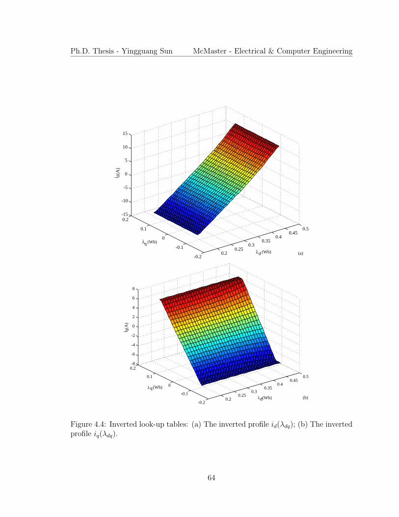
Ph.D. Thesis - Yingguang Sun McMaster - Electrical & Computer Engineering
0.20.25
0.30.35
0.40.45
0.5
-0.2
-0.1
0
0.1
0.2-15
-10
-5
0
5
10
15
d (Wb)
q (Wb)
i d
(A)
0.20.25
0.30.35
0.40.45
0.5
-0.2
-0.1
0
0.1
0.2-8
-6
-4
-2
0
2
4
6
8
d
(Wb)
q (Wb)
i q
(A)
(a)
(b)
Figure 4.4: Inverted look-up tables: (a) The inverted profile id(λdq); (b) The invertedprofile iq(λdq).
64

Ph.D. Thesis - Yingguang Sun McMaster - Electrical & Computer Engineering
+-
R
sT
1/Z
1LUT
1/Z
+
( )dqu k
( )dqi k
( 1)dqk
+
( 1)dqi k
( )e
A
Figure 4.5: Block diagram of the nonlinear machine model dynamics with inverseLUTs.
I is the identity matrix and Y =
[0 −1
1 0
]. The dynamic equations in (4.5) avoid
numerical differentiation of the flux values and hence improve numerical behaviors.
4.3 Experimental Test Bench of Prototype IPM
Motor Drives
In order to validate the proposed speed and position estimation algorithms in this
thesis, an IPMSM drives test bench was set up in the laboratory, which is shown
in Figure 4.6. The Silicon Carbide MOSFET inverter and the MicroAutoBox II are
used for driving the prototype IPM motor. The YASKAWA A-1000 AC Drives is
employed as the controller of the 5 KW dyno induction machine.
65

Ph.D. Thesis - Yingguang Sun McMaster - Electrical & Computer Engineering
IPMDyno
Machine
Dyno
Controller
MicroAutoBox II
SiC MOSFET
Inverter
Figure 4.6: Prototype IPMSM drives test bench.
4.3.1 Silicon Carbide MOSFET Inverter
In recent years, the wide-bandgap semiconductors devices, such as silicon carbide
(SiC), are being more considered in the AC motor drives in the automobile indus-
try. The SiC semiconductors outperform with their fast switching capability, which
reduces the interlock time. Moreover, using high frequency SiC power devices in the
AC motor drives make it possible to operate the drive system with higher PWM fre-
quency, which increases the control system bandwidth. Additionally, it reduces the
values of inductors and capacitors used in the power inverter, which lead to a smaller
inverter size compared with the silicon semiconductor based counterparts (Shirabe
et al., 2014; Zhang et al., 2015).
In the prototype motor drive test bench, a 30 KW SiC MOSFET inverter shown in
Figure 4.7 is utilized in the drive system. The rated DC link voltage of the inverter is
800 V and the rated output phase current is 30 A. The maximum switching frequency
66

Ph.D. Thesis - Yingguang Sun McMaster - Electrical & Computer Engineering
Figure 4.7: Prototype SiC MOSFET inverter.
is up to 100 KHz (Eull et al., 2016).
4.3.2 MicroAutoBox II
MicroAutoBox II is the second generation of dSPACE’s professional and robust stand-
alone prototyping unit which provides universal development system for automobile
applications and other industrial applications. It’s capable of operating without user
intervention (like an ECU) and can be applied for many fast response control pro-
totyping applications such as powertrain, chassis control, body control and electric
drives control, etc (dSPACE GmbH, 2013).
The MicroAutoBox II used in the prototype motor drive system consists of the
DS1401 base board and I/O board 1512/1513. The built in Real Time Interface
(RTI) library provides the link between MicroAutoBox II and the development soft-
ware Matlab/Simulink. It provides a blockset that implements the functionality and
67

Ph.D. Thesis - Yingguang Sun McMaster - Electrical & Computer Engineering
Figure 4.8: RTI Blockset in Simulink.
I/O capability of MicroAutoBox II in the Simulink model (dSPACE GmbH, 2013;
dSPACE, 2014) . The RTI of DS1401/1512/1513 is shown in Figure 4.8. Figure
4.9 shows the working environment of the prototype motor control system using the
experimental software ControlDesk Next Generation.
4.3.3 Dyno Machine Controller
The YASKAWA A-1000 Drive is utilized as the dyno induction machine controller in
the prototype motor drive system. The A-1000 Drive is a full featured drive which
provides close loop and open loop vector control for both permanent magnet machine
and induction machine (YASKAWA, 2014). The control mode can be switched among
speed control, torque control and position control easily and the control reference
signals can be received via CAN, USB and analog input. In the prototype drive
system, the induction machine is controlled in speed mode and the speed reference
is the analog signal transmitted from MicroAutoBox II to A-1000. In this way, the
68

Ph.D. Thesis - Yingguang Sun McMaster - Electrical & Computer Engineering
Figure 4.9: Experimental software ControlDesk Next Generation.
speed and torque references of the two motors are both provided by ControlDesk
simultaneously.
4.3.4 High Accuracy Position Sensor
High accuracy position sensors are necessary for providing accurate measurements
of the actual speed and position in validation of the sensorless methods. Hence,
a fixed resolution incremental encoder with 80000 pulses per mechanical revolution
is installed on the extended shaft of the prototype IPM motor. The position mea-
surement resolution is 0.0225 electrical degree. The encoder interface is internally
implemented in the MicroAutoBox II I/O board for logging the speed and position
information into the control system.
69

Ph.D. Thesis - Yingguang Sun McMaster - Electrical & Computer Engineering
4.4 Conclusions
In this chapter, the novel nonlinear prototype IPM motor model relying on the
current-flux linkage profiles are introduced. The original flux-current profiles were
measured experimentally and were inverted to current-flux profiles by employing the
proposed LUTs inversion method using nonlinear optimization. The new model with
inverted LUTs avoids numerical differentiation of the flux linkage hence improves the
dynamic performance, which is beneficial for the simulation validation of the pro-
posed initial position estimation method. Additionally, the overview of experimental
test bench has been introduced as well. The features of the key components of the
prototype drive system have been explained in detail.
70

Chapter 5
Proposed Nonlinear Optimization
Based Initial Position Estimation
at Startup and Standstill
5.1 Introduction
This chapter proposes a nonlinear optimization based method for initial position es-
timation. In this method, a cost function is defined based on the voltage equations
in α-β axes. Terminal quantities (voltage and current) are employed as inputs of the
cost function and the knowledge of initial rotor position is extracted by minimizing
the cost function. Three steps are needed for fast and accurate initial position esti-
mation, as shown in Figure 5.1 and Figure 5.2. In Step I, a series short pulse voltage
vectors are injected in α-β axes and the resulting current samples are recorded. The
location of the d axis can be identified by searching the minimum of the cost function.
Since the machine performs two periods in one electrical cycle, there are two local
71

Ph.D. Thesis - Yingguang Sun McMaster - Electrical & Computer Engineering
Step I: Pulse voltage
injection in stationary
reference frame
Optimization
using Gi
u
i
Step II: Pulse voltage
injection in estimated
rotor reference frame
Generalized
polarity
detection
method
u
i
1
+
ˆcomp
+
Optimization
using Gl
Step III: Continusous
voltage injection in
estimated rotor
reference frame
2
Inv. park
transform
u
i
u
iPhase Locked
Loop
1/z
1/z
Optimization Based Estimator
Figure 5.1: Block diagram of the proposed optimization based initial position esti-mator.
minimums in the cost function. In order to guarantee a robust position estimation,
a generalized approach to polarity detection which exploits asymmetries in machine
specific differential inductance profiles in d axis is employed as Step II. This approach
leads to a more robust estimation of the polarity that is less sensitive to measurement
noise and can operate with lower resulting currents. After Step I and II, the expected
initial position θ2 is roughly estimated. In order to improve the estimation accuracy,
continuous sinusoidal voltage is injected in estimated d axis in Step III. A modified
cost function is minimized based on the injected voltage and resulting current. Faster
convergence is achieved compared with demodulation based method and Step III can
be easily integrated with running state speed and position estimation.
72

Ph.D. Thesis - Yingguang Sun McMaster - Electrical & Computer Engineering
Step I
aV
aI
5 sT 10 sT 5 sT
Step II
4 sT 8 sT 4 sT
Step III
2ms
Figure 5.2: Screenshot of the scope, voltage injection procedures in initial positionestimation.
5.2 Pulse Voltage Injection for Position Estima-
tion
The discrete voltage equations of IPM motors in d-q frame are
[ud(k)
uq(k)
]=
1
Ts
[Ld 0
0 Lq
]([id(k + 1)
iq(k + 1)
]−
[id(k)
iq(k)
])(5.1)
− ωe(k)
([0 Lq
−Ld 0
][id(k)
iq(k)
]−
[0
λpm
]),
in which the compensated voltages that subtract the voltage drops on the phase
resistance in d-q frame are calculated by udq = udq −Rsidq (Sun et al., 2015).
The machine shaft is not rotating in initial position estimation, i.e. ωe = 0. The
73
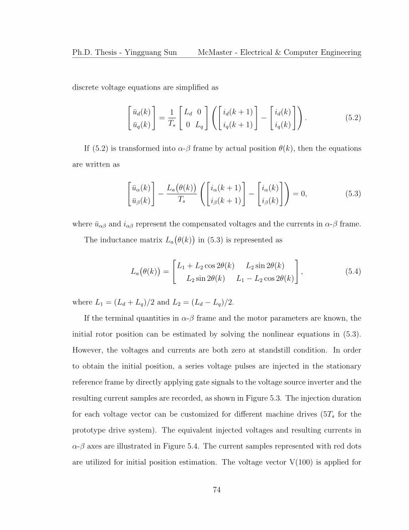
Ph.D. Thesis - Yingguang Sun McMaster - Electrical & Computer Engineering
discrete voltage equations are simplified as
[ud(k)
uq(k)
]=
1
Ts
[Ld 0
0 Lq
]([id(k + 1)
iq(k + 1)
]−
[id(k)
iq(k)
]). (5.2)
If (5.2) is transformed into α-β frame by actual position θ(k), then the equations
are written as
[uα(k)
uβ(k)
]−La(θ(k)
)Ts
([iα(k + 1)
iβ(k + 1)
]−
[iα(k)
iβ(k)
])= 0, (5.3)
where uαβ and iαβ represent the compensated voltages and the currents in α-β frame.
The inductance matrix La(θ(k)
)in (5.3) is represented as
La(θ(k)
)=
[L1 + L2 cos 2θ(k) L2 sin 2θ(k)
L2 sin 2θ(k) L1 − L2 cos 2θ(k)
], (5.4)
where L1 = (Ld + Lq)/2 and L2 = (Ld − Lq)/2.
If the terminal quantities in α-β frame and the motor parameters are known, the
initial rotor position can be estimated by solving the nonlinear equations in (5.3).
However, the voltages and currents are both zero at standstill condition. In order
to obtain the initial position, a series voltage pulses are injected in the stationary
reference frame by directly applying gate signals to the voltage source inverter and the
resulting current samples are recorded, as shown in Figure 5.3. The injection duration
for each voltage vector can be customized for different machine drives (5Ts for the
prototype drive system). The equivalent injected voltages and resulting currents in
α-β axes are illustrated in Figure 5.4. The current samples represented with red dots
are utilized for initial position estimation. The voltage vector V(100) is applied for
74
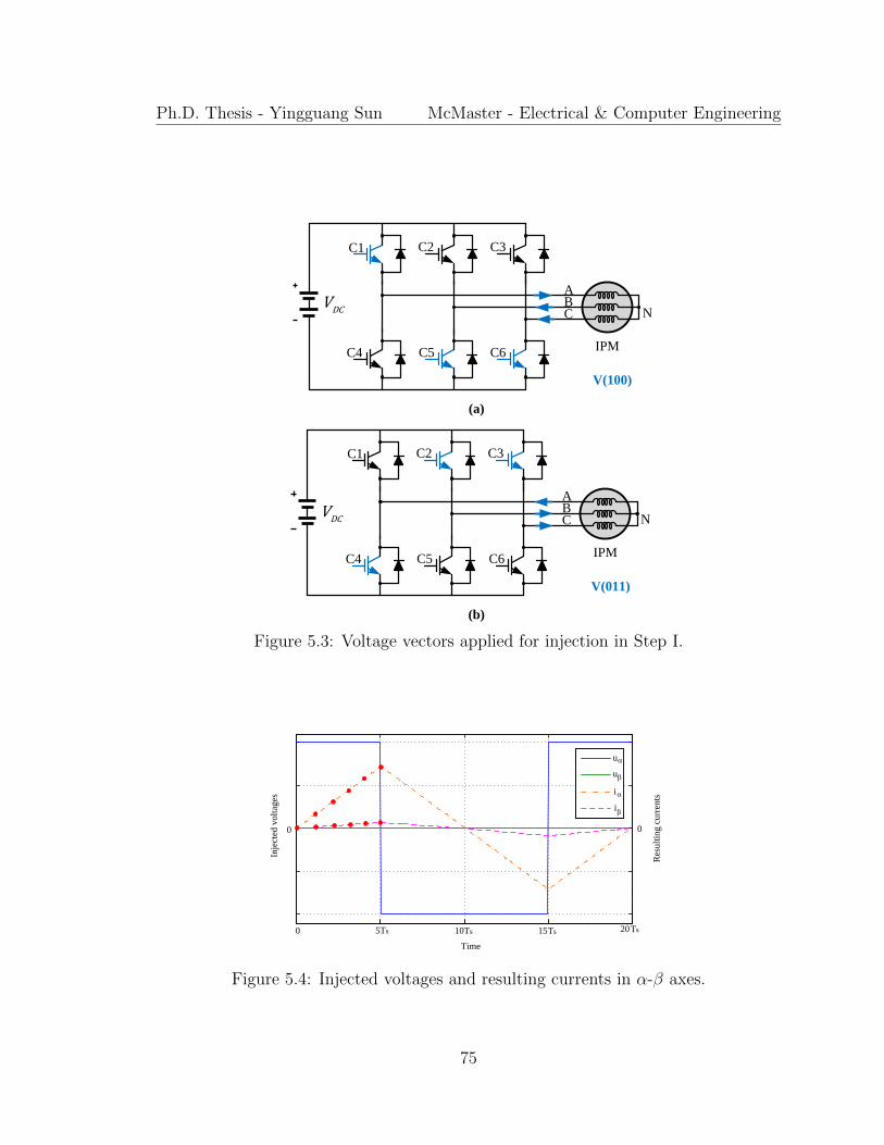
Ph.D. Thesis - Yingguang Sun McMaster - Electrical & Computer Engineering
ABC
C1 C2 C3
C4 C5 C6IPM
N
V(011)
(a)
(b)
ABC
C1 C2 C3
C4 C5 C6IPM
NDCV
V(100)
DCV
Figure 5.3: Voltage vectors applied for injection in Step I.
0 10 15 20
Time
0
u
u
i
i
0
5Ts Ts Ts Ts
Inje
cted
vo
ltag
es
Res
ult
ing
cu
rren
ts
Figure 5.4: Injected voltages and resulting currents in α-β axes.
75

Ph.D. Thesis - Yingguang Sun McMaster - Electrical & Computer Engineering
5Ts and then the vector V(011) and V(100) are applied for 10Ts and 5Ts respectively
to null the current response and balance the rotor movement (Sun et al., 2015).
Moreover, the proposed injection scheme is also shown in Figure 5.2 which is the
screenshot of the scope in experiment. The yellow voltage Va is the voltage between
phase A terminal and the negative bus bar of the inverter (voltage across the lower
switch in phase A) and the green current Ia is the measured phase A current. They
are the direct measurements which can illustrate the injection scheme and resulting
currents in α-β frame. The available DC link voltage VDC in the prototype drive
system is 300 V. When the voltage vector V(100) is applied, the Va = 300V and the
equivalent injected voltage in α axis is 200 V. The current samples used for position
estimation are also marked with red dots in Figure 5.2. The current responses in the
other two phases are also used for position estimation and the three phase current
samples are transformed into α-β frame by Clark Transformation (Sun et al., 2015).
If the cost function is defined in
minimizeθ
Gi(θ) =m∑k=1
∥∥∥uαβ(k)− La(θ)
Ts
(iαβ(k + 1)− iαβ(k)
)∥∥∥2 (5.5)
based on (5.3), then the cost is zero if the actual initial position is utilized. However,
only estimated position exists in the sensorless control system. The cost will be zero
if the estimated initial position is exactly the actual initial position, otherwise the
cost will not be zero. The parameter m indicates that the injection duration for each
voltage vector lasts for mTs. Since the rotor position is constant in initial position
estimation, the θ is used instead of θ(k) for different current samples.
Figure 5.5 shows the plot of Gi(θ) versus position estimation errors at different
initial positions using experimental data. Each data set refers to a certain initial
76

Ph.D. Thesis - Yingguang Sun McMaster - Electrical & Computer Engineering
-400 -300 -200 -100 0 100 200 300 4000
10
20
30
40
50
60
Position estimation error (elec deg)
Cost
0
60
120
180
240
300
360180 180
Figure 5.5: Plot of Gi(θ) versus position estimation errors at different initial positionsfor m = 1 based on experimental data.
position and is represented by a specific color and marker. From the figure, it is clear
that Gi(θ) has two local minimums which locate around 0 error and 180 error in
one electrical period at different initial positions. The cost function Gi(θ) decreases
as the estimated position approaches to the two local minimums. The expected local
minimum located at 0 position estimation error indicates that the positive direction
of the estimated d axis aligns with the north magnetic pole. The other local minimum
located at 180 error implies that the positive direction of the estimated d axis aligns
with the south magnetic pole, which is unexpected. The initial position is estimated
by searching the minimum of (5.5) and this nonlinear least-squares optimization can
be easily solved by employing line search approaches (Luenberger and Ye, 2008).
However, the nonlinear optimization starts from an initial guess which can be
closer to either the expected local minimum or the unexpected one. The failure of
identifying the expected minimum will lead to the search algorithm converging to
the unexpected local minimum. Hence, magnetic polarity detection is needed to
guarantee the robustness of the initial position estimation.
77

Ph.D. Thesis - Yingguang Sun McMaster - Electrical & Computer Engineering
5.3 Generalized Polarity Detection Method
As introduced in Section 3.5.2, existing magnetic polarity detection methods mostly
rely on the magnetic saturation effect of the stator iron. The flux linkage in d axis
saturates under positive current, which can be observed from Figure 4.1 (b). The d
axis flux linkage profiles of the prototype machine were measured from experiments.
In dual voltage pulses injection based method in 3.5.2, the current needed to detect
reliable saturation can be close to or higher than the rated current and requires an
inverter with high power rating in some machines. Moreover, checking two or three
current peak values is not robust in detecting the polarity if the measurement noise
and modeling inaccuracy are taken into consideration. In this thesis, in order to detect
the magnetic polarity robustly, the d axis flux linkage profile λd(id, 0) was measured
at different id when iq = 0 from experiment with typical motor drives components
(Cintron-Rivera et al., 2012). Then the d axis differential inductance profile `dd(id, 0)
is utilized, which is calculated as `dd(id, 0) = ∂λd(id, 0)/∂id. Figure 5.6 shows the
experimental obtained d axis differential inductance profile used in the generalized
polarity detection method. The differential inductance profile is implemented as look-
up tables in the real time experimental tests.
The calculated differential inductance Ldiffδ can be obtained from the injected
voltages and induced currents at each sampling time in
Ldiffδ (j) =∆λδ(j)
∆iδ(j)=
Tsuδ(j − 1)
iδ(j)− iδ(j − 1)=
TsVpoliδ(j)− iδ(j − 1)
(5.6)
where Vpol denotes the magnitude of the compensated injection voltage subtracting
the resistive voltage drop and ∆iδ represents the difference between two consecutive
78

Ph.D. Thesis - Yingguang Sun McMaster - Electrical & Computer Engineering
-10 -5 0 5 10
0.009
0.0095
0.01
0.0105
0.011
0.0115
0.012
0.0125
0.013
0.0135
0.014
dd
(id
, 0
) (H
)
id (A)
Figure 5.6: Experimental obtained d axis differential inductance profile `dd(id, 0).
current samples. Since the voltage vectors are injected in δ axis, the current compo-
nents in γ axis are negligible. The current iδ(j) is measured at each sample time and
Ldiffδ (j) is calculated by (5.6) accordingly (Sun et al., 2015).
The injection scheme for magnetic polarity detection is shown in Figure 5.7. Short
voltage pulses are injected in δ axis with the same injection scheme in Step I. The
injection magnitude is also 200 V and the injection duration is 4Ts for each voltage
pulse. Since the voltage and current used for polarity detection are in the estimated
d axis, they can not be exactly reflected by the scope screenshot shown in Figure 5.2
with Va and Ia. But the injection scheme and the resulting current waveforms in δ
axis can still be illustrated by Figure 5.2. The current samples in purple dots are used
for polarity detection. In Figure 5.2, eight sets of data (iδ(j), Ldiffδ (j)), j = 1 . . . 8 are
recorded. If the estimated d axis aligns with the north pole, then Ldiffδ (j) matches
with differential inductance profile `dd(iδ(j), 0) in Figure 5.6. If the estimated d axis
aligns with the south pole, Ldiffδ (j) matches with the profile `dd(−iδ(j), 0).
In general, if each voltage pulse lasts for nTs, then the difference between Ldiffδ (j)
79
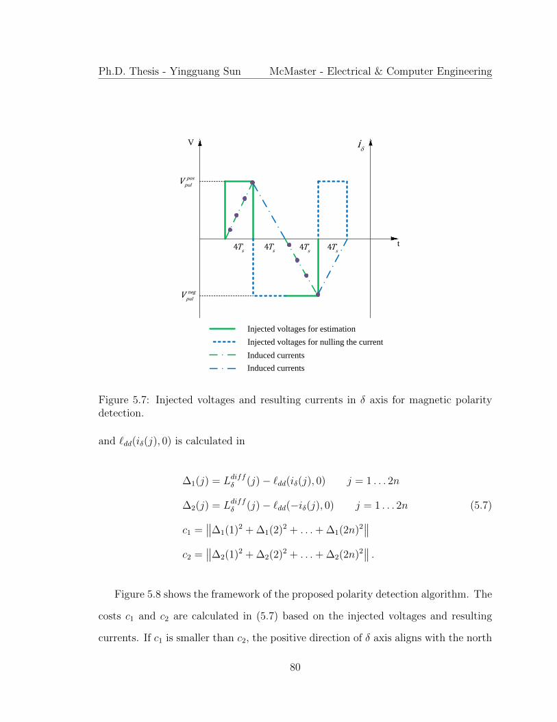
Ph.D. Thesis - Yingguang Sun McMaster - Electrical & Computer Engineering
t
V
pos
pulV
neg
pulV
4sT
i
Injected voltages for estimation
Induced currents
Injected voltages for nulling the current
Induced currents
4sT 4
sT 4
sT
Figure 5.7: Injected voltages and resulting currents in δ axis for magnetic polaritydetection.
and `dd(iδ(j), 0) is calculated in
∆1(j) = Ldiffδ (j)− `dd(iδ(j), 0) j = 1 . . . 2n
∆2(j) = Ldiffδ (j)− `dd(−iδ(j), 0) j = 1 . . . 2n (5.7)
c1 =∥∥∆1(1)2 + ∆1(2)2 + . . .+ ∆1(2n)2
∥∥c2 =
∥∥∆2(1)2 + ∆2(2)2 + . . .+ ∆2(2n)2∥∥ .
Figure 5.8 shows the framework of the proposed polarity detection algorithm. The
costs c1 and c2 are calculated in (5.7) based on the injected voltages and resulting
currents. If c1 is smaller than c2, the positive direction of δ axis aligns with the north
80

Ph.D. Thesis - Yingguang Sun McMaster - Electrical & Computer Engineering
Voltage pulses
injection
Record the current responses
Calculate the differential inductances
2 1ˆ ˆ
2 1ˆ ˆ 180
Y
N<
Calculate and1c
2c
1c
2c
Figure 5.8: Framework of the proposed polarity detection method.
pole and the estimated position θ1 from Step I is correct. While if c1 is larger than
c2, the positive direction of δ axis aligns with the south pole and θ1 has to be added
by 180 (Sun et al., 2015).
In Figure 5.2, the selected magnitude and duration of each injected voltage vector
in Step I and II are customized for the prototype IPM motor drive system. Generally,
the magnitude of the resulting current due to injected voltage is determined by the
available DC link voltage, sampling time and motor parameters. In Step I, the result-
ing current peak changes with respect to the initial position because the equivalent
inductances in α-β axes are position dependent. The maximum current peak in α
axis happens when α axis aligns with d axis. The current peak will be smaller at
other initial positions, i.e. the current peak is smaller when α axis aligns with q axis
due to the larger Lq. Hence, the resulting current peak Ipeak in Step I and II can be
81

Ph.D. Thesis - Yingguang Sun McMaster - Electrical & Computer Engineering
estimated by
Ipeak ≤mTsVeqLd
, (5.8)
where m and Veq denote the injection duration of each voltage vector and the equiv-
alent injected voltage in α axis or δ axis. The Ld value used in (5.8) comes from the
experimental obtained d axis differential inductance profile mentioned above. Theo-
retically, the estimation method in Step I should work when m ≥ 1. In practice, the
injection duration needs to be increased to achieve robust initial position estimation.
A reasonable first estimate of Ipeak can be 50% of the rated current and the calculated
m can be adjusted in simulation and experimental tests based on this initial estimate.
The injection duration m ∈ [3 6] in Step I for the prototype drive system. If m < 3,
robust estimation can not be guaranteed. If m ≥ 6, the Ipeak is close to and larger
than the rated current. The 5Ts injection duration is selected by considering both the
estimation accuracy and the Ipeak value. In Step II, the robust detection of polarity
can be achieved when m ≥ 4. Since the polarity detection is to make a decision
whether compensating 180 or not, no further accuracy issue needs to be considered.
Therefore, the injection duration for polarity detection is chosen as 4Ts. Hence, the
proposed methods in Step I and II are generalized for different IPMSM drives but the
optimal injection scheme needs to be determined distinctly for a specific drive system
based on the strategy mentioned above.
82
Ph.D. Thesis - Yingguang Sun McMaster - Electrical & Computer Engineering
5.4 Continuous Sinusoidal Voltage Injection for Po-
sition Estimation
After Step I and II, the initial position with polarity correction has already been
obtained, which is θ2 in Figure 5.1. The benefits of the pulse injection based method
is its fast estimation capability. However, the assumption that the injected voltage
magnitudes are kept constant regardless of the injection direction can’t be guaranteed
due to the inverter nonlinearities. Using calculated voltages instead of directly mea-
sured ones will affect the estimation accuracy (Antonello et al., 2015). Moreover, the
position needs to be continuously estimated at standstill condition besides machine
startup, i.e. rotor is locked mechanically. Hence, a continuous voltage injection based
method using nonlinear optimization is proposed for position estimation at standstill
condition and for easier integration with the speed and position estimation at running
state.
Based on (5.1), a modified cost function
minimizeθ(k),ω(k)
Gl
(θ(k), ωe(k)
)=
∥∥∥∥∥uαβ(k)−La(θ(k)
)Ts
(T(∆θ(k)
)iαβ(k + 1)− iαβ(k)
)+ ωe(k)
(Lb(θ(k)
)iαβ(k) + λpm
[sin θ(k)
− cos θ(k)
])∥∥∥∥∥2
+K1
(θ(k)− θ(k − 1)
)2(5.9)
+K2
(ωe(k)− ωe(k − 1)
)2is derived by utilizing the similar idea in deducing the cost function (5.5). The position
difference between two consecutive sample times is calculated as ∆θ(k) = Tsωe(k).
In initial position estimation, ωe(k) equals to zero. The transformation T (∆θ(k)) is
83

Ph.D. Thesis - Yingguang Sun McMaster - Electrical & Computer Engineering
position error (elec deg)
spee
d e
rror
(rpm
)
0 50 100 150 200 250 300
-300
-200
-100
0
100
200
300
50
100
150
200
250
300
350
400
450
500
550
(0,0)
Figure 5.9: Contour plot of the cost function (5.9) at standstill condition.
represented in
T(∆θ(k)
)=
cos(∆θ(k)
)sin(∆θ(k)
)− sin
(∆θ(k)
)cos(∆θ(k)
) . (5.10)
At standstill condition, continuous sinusoidal voltages are injected in estimated d
axis, which is shown as Step III in Figure 5.2. The voltage and current information are
used for estimation in each sample time. The previous estimated speed and position
are used as starting points for the next optimization. The contour plot of (5.9) is
depicted in Figure 5.9.
In Figure 5.9, only one minimum in the origin is obtained in one electrical period,
which indicates the correct speed and position estimation. Therefore, the speed and
position estimation becomes an online nonlinear optimization problem with two de-
cision variables and the estimation can be achieved by minimizing the cost function
(5.9). If the previous estimation is known in (5.9), the optimization will finally reach
to the expected minimum with finite iterations. In this way, the speed and position
84

Ph.D. Thesis - Yingguang Sun McMaster - Electrical & Computer Engineering
are continuously estimated in Step III. A PLL is implemented in series with the op-
timization based position estimator in Step III as a filter. More analysis of the cost
function (5.9), and the nonlinear optimization based speed and position estimation
at running state will be illustrated in Chapter 6.
5.5 Simulation Verifications
The proposed initial position estimation algorithms were modeled and simulated in
MATLAB/SIMULINK before experimental verification. The novel nonlinear machine
model introduced in Chapter 4 is employed for accurately simulating the initial posi-
tion estimation performance. The switching frequency and sampling frequency were
both set to 10 kHz and the DC link voltage was 300 V. The injection scheme used
in Step I and II is identical with Figure 5.2. For the continuous injection in Step III,
the magnitude of the sinusoidal voltage was 70 V and the injection frequency was 500
Hz.
Figure 5.10 illustrates the simulation results of the initial position estimation when
the actual position was 41.5 electrical degree. The green shade represents Step I and
Step II which last for 4.1 ms in total. After position estimation and polarity detection,
the estimation error is 10. This error comes from the mismatch between the constant
parameter estimation model and real nonlinear machine model. Then the continuous
sinusoidal voltage is injected in Step III and the final position estimation error is
−0.5 electrical degree, as shown in Figure 5.10 (b). In this test, the compensation
of the polarity detection is 0 because c1 is smaller than c2, which is illustrated in
Figure 5.10 (c).
Figure 5.11 shows the position estimation results when the actual position was
85

Ph.D. Thesis - Yingguang Sun McMaster - Electrical & Computer Engineering
0 0.05 0.1 0.15 0.2 0.25 0.3 0.35 0.40
10
20
30
40
50
Time (s)
Po
siti
on
s (e
lec
deg
)
Estimated positionActual position
(a)
Step I and II,
4.1ms in total
Step III, keep
estimating at
standstill
0.5
41.5
0 0.05 0.1 0.15 0.2 0.25 0.3 0.35 0.4
0
10
20
30
40
Time (s)
Po
siti
on
est
imat
ion
err
or
(ele
c d
eg)
(b)
0 0.05 0.1 0.15 0.2 0.25 0.3 0.35 0.40
2
4
6
8x 10
-3
Time (s)
Co
sts
in p
ola
rity
det
ecti
on
c1
c2
(c)
Figure 5.10: Simulation results on initial position estimation at 41.5: (a) actual andestimated positions; (b) position estimation error; (c) c1 and c2 in polarity detection.
250. After position estimation there exists 180 error in the estimation results, which
can be reflected by the fact that c1 is larger than c2. This error is compensated by
the proposed polarity detection algorithm and Figure 5.11 (a) illustrates the position
estimation results. The position estimation error in this case is 0.8 electrical degree
after Step III.
In Step III, the continuous voltage injection is used and the modified cost function
(5.9) is employed in position estimation. Since both speed and position are decision
variables in the optimization, the same idea can be extended to speed and position
86

Ph.D. Thesis - Yingguang Sun McMaster - Electrical & Computer Engineering
0 0.05 0.1 0.15 0.2 0.25 0.3 0.35 0.40
50
100
150
200
250
300
Time (s)
Posi
tions
(ele
c deg
)
Actual positionEstimated position
Step I and II,
4.1ms in total
Step III, keep
estimating at
standstill
0.8
250
0 0.05 0.1 0.15 0.2 0.25 0.3 0.35 0.4-100
0
100
200
300
Time (s)
Posi
tion e
stim
atio
n e
rror
(ele
c deg
)
(a)
(b)
180
0 0.05 0.1 0.15 0.2 0.25 0.3 0.35 0.40
1
2
3
4
5x 10
-3
Time (s)
Cost
s in
pola
rity
det
ecti
on
c1c2
(c)
Figure 5.11: Simulation results on initial position estimation at 250: (a) actual andestimated positions; (b) position estimation error; (c) c1 and c2 in polarity detection.
estimation at low speed conditions. Figure 5.12 illustrates the speed and position
estimation from standstill condition to low speed operations. The speed and position
estimation both works well at standstill condition and low speed.
87

Ph.D. Thesis - Yingguang Sun McMaster - Electrical & Computer Engineering
0 0.5 1 1.5 2 2.5 3 3.5 40
100
200
300
400
Time (s)
Po
siti
on
s (e
lec
deg
)
Actual position
Estimated position
0 0.5 1 1.5 2 2.5 3 3.5 4-5
0
5
10
15
20
25
Time (s)
Po
siti
on
est
imat
ion
err
or
(ele
c d
eg)
(a)
(b)
0 0.5 1 1.5 2 2.5 3 3.5 4-20
0
20
40
60
Time (s)
Sp
eed
s (r
pm
)
Actual speedEstimated speed
(c)
Figure 5.12: Simulation results on integration of speed and position estimation atstandstill and low speed: (a) actual and estimated positions; (b) position estimationerror; (c) actual and estimated speeds.
5.6 Experimental Verifications
5.6.1 Experimental Results on Initial Position Estimation
The proposed initial position estimation approach was tested with the experimental
test bench shown in Figure 4.6. The IPMSM drives parameters and injection scheme
are identical with simulation test conditions shown in Section 5.5.
Figure 5.13 illustrates the estimation results when the real measured position was
88

Ph.D. Thesis - Yingguang Sun McMaster - Electrical & Computer Engineering
0 0.05 0.1 0.15 0.2 0.25 0.3 0.35 0.40
10
20
30
40
50
Time (s)
Posi
tions
(ele
c deg
)
Measured position
Estimated positionStep I and II,
4.1ms in total
Step III, keep
estimating at
standstill
0 0.05 0.1 0.15 0.2 0.25 0.3 0.35 0.4
0
10
20
30
40
Time (s)
Posi
tion e
stim
atio
n e
rror
(ele
c deg
)
1.5
41.5
(a)
0 0.05 0.1 0.15 0.2 0.25 0.3 0.35 0.40
2
4
6
8x 10
-3
Time (s)
Cost
s in
pola
rity
det
ecti
on
c1
c2
(b)
(c)
Figure 5.13: Experimental results on initial position estimation at 41.5: (a) mea-sured and estimated positions; (b) position estimation error; (c) c1 and c2 in polaritydetection.
41.5 electrical degree. The green shade represents Step I and Step II which last for
4.1 ms in total. After position estimation and polarity detection, the estimation error
is 20. This error is larger compared with simulation. This is due to the involvement
of measurement noise and inverter nonlinearities. Then the continuous sinusoidal
voltage is injected and the final position estimation error is 1.5 electrical degree, as
shown in Figure 5.13 (b). In this test, the compensation of the polarity detection is 0
because c1 is smaller than c2, which is illustrated in Figure 5.13 (c). The experimental
89

Ph.D. Thesis - Yingguang Sun McMaster - Electrical & Computer Engineering
0 0.05 0.1 0.15 0.2 0.25 0.3 0.35 0.40
50
100
150
200
250
300
Time (s)
Po
siti
on
s (e
lec
deg
)
Measured positionEstimated positionStep I and II,
4.1ms in total
Step III, keep
estimating at
standstill
250
0 0.05 0.1 0.15 0.2 0.25 0.3 0.35 0.4-100
0
100
200
300
Time (s)
Po
siti
on
est
imat
ion
err
or
(ele
c d
eg)
1800.2
(a)
(b)
0 0.05 0.1 0.15 0.2 0.25 0.3 0.35 0.40
2
4
6
8x 10⁻³
Time (s)
Co
sts
in p
ola
rity
det
ecti
on
c1
c2
(c)
Figure 5.14: Experimental results on initial position estimation at 250: (a) mea-sured and estimated positions; (b) position estimation error; (c) c1 and c2 in polaritydetection.
results match with the simulation very well.
Figure 5.14 shows the position estimation results when the real position was 250.
After Step I there exists 180 error in the estimation results, which can be reflected
by the fact that c1 is larger than c2. This error is compensated by the proposed
polarity detection algorithm and Figure 5.14 (a) illustrates the position estimation
results. The position estimation error in this case is 0.2 electrical degree after Step
III, which is observed similarly in the simulation results.
90

Ph.D. Thesis - Yingguang Sun McMaster - Electrical & Computer Engineering
0 0.5 1 1.5 2 2.5 3 3.5 40
100
200
300
400
Time (s)
Po
siti
on
s (e
lec
deg
)
Estimated position
Measured position
0 0.5 1 1.5 2 2.5 3 3.5 4-5
0
5
10
15
20
25
Time (s)
Po
siti
on
est
imat
ion
err
or
(ele
c d
eg)
(a)
(b)
0 0.5 1 1.5 2 2.5 3 3.5 4-20
0
20
40
60
Time (s)
Sp
eed
s (r
pm
)
Estimated speed
Measured speed
(c)
Figure 5.15: Experimental results on integration of speed and position estimationat standstill and running state: (a) measured and estimated positions; (b) positionestimation error; (c) measured and estimated speeds.
Similarly in Figure 5.12, the integration of standstill estimation and low speed
estimation was tested in experiments. The experimental results are shown in Figure
5.15. It is concluded that the optimization based method is unified at standstill
condition as well as low speed operations. More details about running state estimation
will be shown in Chapter 6.
91

Ph.D. Thesis - Yingguang Sun McMaster - Electrical & Computer Engineering
0 50 100 150 200 250 300-40
-20
0
20
40
Different initial positions in one electrical peroid (elec deg)
Po
siti
on
est
imat
ion
err
ors
(el
ec d
eg)
After Step I and II
After Step III
345
Figure 5.16: Experimental results, position estimation errors of pulse voltage injectionand continuous sinusoidal voltage injection.
5.6.2 Accuracy Comparison Between Pulse Voltage Injection
and Continuous Sinusoidal Injection
The benefit of the pulse voltage injection based initial position estimation is its fast
response. In the experimental tests illustrated above, the initial position was roughly
achieved with only 4.1 ms. However, the estimation accuracy can’t be guaranteed
due to the machine and inverter nonlinearities, as mentioned in Section 5.4. Figure
5.16 shows the comparison of the estimation accuracies between pulse injection and
continuous injection. The average estimation error of the pulse injection is 11.52
while the final average estimation error decreases to 0.91 electrical degree after the
sinusoidal injection and the PLL are involved in Step III.
5.7 Conclusions
In this chapter, an optimization based initial position estimation algorithm is pro-
posed. A cost function is defined and the position can be estimated by searching
92

Ph.D. Thesis - Yingguang Sun McMaster - Electrical & Computer Engineering
the minimum of the cost function. Three steps which employ different voltage injec-
tions are utilized in the fast and accurate estimation of initial position. The pulse
voltage injection for position estimation benefits from its fast response, but polarity
detection and accuracy improvements are needed. The proposed polarity detection
method generalizes the polarity detection techniques for different IPM motor drives.
The polarity can be detected once the differential inductance profile is known. Com-
pared with methods relying solely on saturation, the proposed method requires lower
currents to reliably determine the polarity. The continuous voltage injection is used
for position estimation at standstill condition after the initial position is roughly
obtained. The involvement of continuous injection in Step III improves the estima-
tion accuracy and proposes a unified solution for integrating the speed and position
estimation at standstill condition and running state.
The feasibility of the proposed initial position estimation method has been investi-
gated and validated with both simulation and experimental tests. The initial position
can be identified within 50 milliseconds and the position estimation accuracy is less
than 1 electrical degree.
93

Chapter 6
Proposed Nonlinear Optimization
Based Speed and Position
Estimation at Running State
6.1 Introduction
This chapter proposes a nonlinear optimization based position and speed estimation
algorithm for wide speed range operations. A cost function based on voltage equa-
tions in the stationary reference frame is employed for speed and position estimation.
The speed and position are both involved in the cost function and they are deci-
sion variables for this nonlinear optimization problem. The speed and position can
be estimated by minimizing the proposed cost function based on measurements of
stator voltages and currents. Since the voltage information is less significant at low
speed and unable to be observed at standstill condition, extra high frequency sinu-
soidal voltages are injected in estimated magnetic axis. Extra regularization terms
94

Ph.D. Thesis - Yingguang Sun McMaster - Electrical & Computer Engineering
α-β
SVM
α-β abc
Trigger
signalsCurrent
controller
Current
controller
IPMSM
SiC MOSFET
inverter
DC link
voltage
Position
estimator
+_
+ _
,u
,i
refi
refi
u
u
u
u
i
i
i
i
abci
abcu
initial
δ-γ
α-β δ-γ
MicroAutoBox II
1/z
++
Variable magnitudes high frequency
voltage injection
Dyno
Dyno
controllerinitial
1/z
Figure 6.1: Block diagram of the proposed nonlinear optimization based sensorlesscontrol system.
are added in the cost function at low speed to improve speed and position estima-
tion quality. A PLL is involved at the output of the position estimator serving as a
filter. In this way, a unified position and speed estimation method is proposed for
wide speed range operation without switching between different position estimation
algorithms at wide speed range. The system block diagram is shown in Figure 6.1.
Analysis on the cost function and convexity under different speeds and positions are
also shown in this chapter. The feasibility of the proposed estimation algorithm is
validated with the prototype IPM motor drive system. Additionally, the parameter
sensitivity analysis of the proposed method is also illustrated both with theoretical
analysis and experimental tests.
95
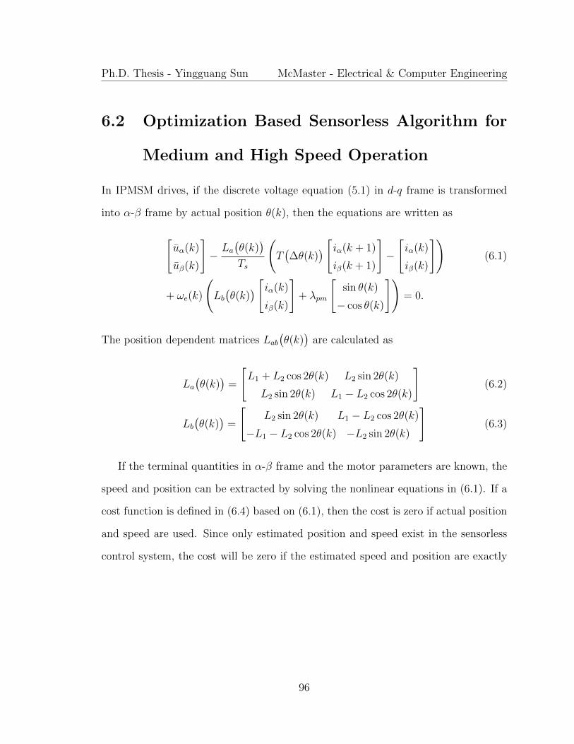
Ph.D. Thesis - Yingguang Sun McMaster - Electrical & Computer Engineering
6.2 Optimization Based Sensorless Algorithm for
Medium and High Speed Operation
In IPMSM drives, if the discrete voltage equation (5.1) in d-q frame is transformed
into α-β frame by actual position θ(k), then the equations are written as
[uα(k)
uβ(k)
]−La(θ(k)
)Ts
(T(∆θ(k)
) [iα(k + 1)
iβ(k + 1)
]−
[iα(k)
iβ(k)
])(6.1)
+ ωe(k)
(Lb(θ(k)
) [iα(k)
iβ(k)
]+ λpm
[sin θ(k)
− cos θ(k)
])= 0.
The position dependent matrices Lab(θ(k)
)are calculated as
La(θ(k)
)=
[L1 + L2 cos 2θ(k) L2 sin 2θ(k)
L2 sin 2θ(k) L1 − L2 cos 2θ(k)
](6.2)
Lb(θ(k)
)=
[L2 sin 2θ(k) L1 − L2 cos 2θ(k)
−L1 − L2 cos 2θ(k) −L2 sin 2θ(k)
](6.3)
If the terminal quantities in α-β frame and the motor parameters are known, the
speed and position can be extracted by solving the nonlinear equations in (6.1). If a
cost function is defined in (6.4) based on (6.1), then the cost is zero if actual position
and speed are used. Since only estimated position and speed exist in the sensorless
control system, the cost will be zero if the estimated speed and position are exactly
96

Ph.D. Thesis - Yingguang Sun McMaster - Electrical & Computer Engineering
the actual ones (Sun et al., 2016).
minimizeθ(k),ω(k)
Gr
(θ(k), ωe(k)
)=
∥∥∥∥∥uαβ(k)−La(θ(k)
)Ts
(T(∆θ(k)
)iαβ(k + 1)− iαβ(k)
)(6.4)
+ ωe(k)
(Lb(θ(k)
)iαβ(k) + λpm
[sin θ(k)
− cos θ(k)
])∥∥∥∥∥2
Figure 6.2 shows the contour plots of the cost function at different speed and
position conditions. The horizontal axis is position estimation error and the vertical
axis is speed estimation error. From the contour plots, it is clear that the cost
decreases as the estimated speed and position approach to the actual speed and
position. The cost function has two local minimums in one electrical period. If the
machine is running at N rpm, the first local minimum locates at the origin. The
speed and position errors are both zero, which indicates the correct estimation. The
second local minimum’s coordinate is (180, -2N rpm) which corresponds to the
negative direction of the magnetic axis. Therefore, the speed and position estimation
at running state becomes an online nonlinear optimization problem with two decision
variables and the estimation can be achieved by minimizing the cost function (6.4).
If the cost function is locally convex and if the initial value of each estimation is
around the expected local minimum, the optimization is able to reach to the expected
local minimum with finite iterations. A cost function is said to be convex if the
second derivative (Hessian) is positive semi-definite in a convex region (Boyd and
Vandenberghe, 2004). However, the analytical demonstration is challenging due to
the complexity of the Hessian of the proposed cost function. A real symmetric matrix
is said to be positive semi-definite if all its eigenvalues are non-negative. In the
97
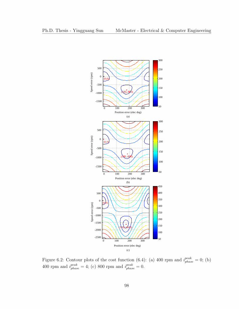
Ph.D. Thesis - Yingguang Sun McMaster - Electrical & Computer Engineering
Position error (elec deg)
Sp
eed
err
or
(rp
m)
0 100 200 300
-1500
-1000
-500
0
500
50
100
150
200
250
300
(a)
Position error (elec deg)
Sp
eed
err
or
(rp
m)
0 100 200 300
-1500
-1000
-500
0
500
50
100
150
200
250
300
(0,0)
(180,-800)
(0,0)
(180,-800)
Position error (elec deg)
Sp
eed
err
or
(rp
m)
0 100 200 300
-2500
-2000
-1500
-1000
-500
0
500
50
100
150
200
250
300
350
400
450
(b)
(c)
(0,0)
(180,-1600)
Figure 6.2: Contour plots of the cost function (6.4): (a) 400 rpm and ipeakphase = 0; (b)
400 rpm and ipeakphase = 4; (c) 800 rpm and ipeakphase = 0.
98

Ph.D. Thesis - Yingguang Sun McMaster - Electrical & Computer Engineering
proposed cost function, the Hessian is a 2 × 2 real symmetric matrix and has two
eigenvalues. The local convexity of the cost function around the two local minimums
is illustrated by plotting the region in which all the eigenvalues of the Hessian are
non-negative. The procedures are: (a) The eigenvalues of the Hessian are calculated
at different speeds and positions with 0.4 degree and 10 rpm intervals; (b) If the
two eigenvalues are both non-negative, the point is recorded and plotted on top of
the contour plot of the cost function; (3) The convex regions then are depicted in
Figure 6.3 and Figure 6.4. The plots were also depicted with the position and speed
intervals as small as 0.1 degree and 1 rpm and the convex regions have the same
envelops with Figure 6.3 and Figure 6.4 but with more points included. The idea
of illustrating the observer convergence with plots or system trajectories has already
been used in literature (Nahid-Mobarakeh et al., 2004, 2007). In Figure 6.3 (b) and
Figure 6.4 (b), the zoomed in convex regions around the expected local minimum are
shown. The convergence of the proposed position estimator is guaranteed if the speed
and position errors are within those regions. Outside these regions, no convergence
guarantees can be issued (Sun et al., 2016).
6.3 Modification of the Cost Function at Low Speed
Operation
Since the back-emf is proportional to the machine speed, the voltage magnitudes in
(6.4) is more significant at higher speed. The size of the local convex region increases
at higher speed due to the increase of the voltages, as illustrated in Figure 6.3 and
Figure 6.4. At very low speed including standstill condition, the cost function Gr in
99
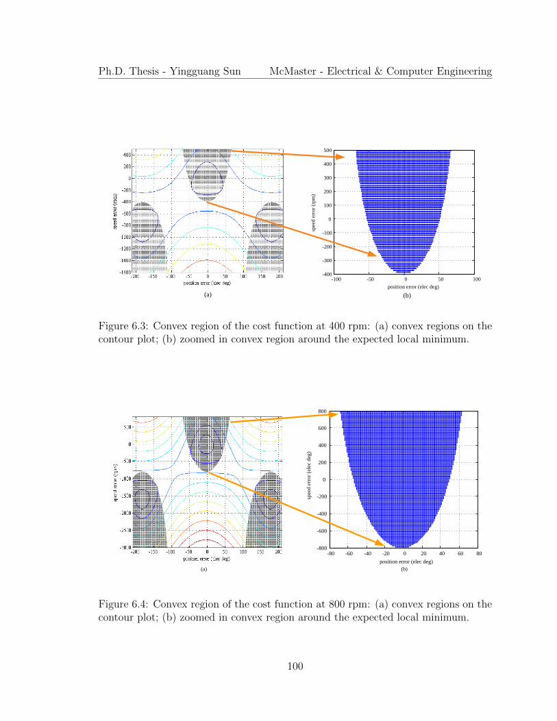
Ph.D. Thesis - Yingguang Sun McMaster - Electrical & Computer Engineering
-100 -50 0 50 100-400
-300
-200
-100
0
100
200
300
400
500
position error (elec deg)
spee
d e
rro
r (r
pm
)
(a) (b)
Figure 6.3: Convex region of the cost function at 400 rpm: (a) convex regions on thecontour plot; (b) zoomed in convex region around the expected local minimum.
-80 -60 -40 -20 0 20 40 60 80-800
-600
-400
-200
0
200
400
600
800
position error (elec deg)
spee
d e
rror
(ele
c deg
)
(a) (b)
Figure 6.4: Convex region of the cost function at 800 rpm: (a) convex regions on thecontour plot; (b) zoomed in convex region around the expected local minimum.
100

Ph.D. Thesis - Yingguang Sun McMaster - Electrical & Computer Engineering
(6.4) is not convex as shown in Figure 6.5 (a) and Figure 6.6 (a). In order to estimate
the speed and position at low speed, high frequency sinusoidal voltages are injected
in δ axis and Gr is modified in
minimizeθ(k),ω(k)
Gl(θ(k), ωe(k)) = Gr
(θ(k), ωe(k)
)+K1
(θ(k)− θ(k − 1)
)2(6.5)
+K2
(ωe(k)− ωe(k − 1)
)2.
Equation (6.5) is the same with the cost function introduced in (5.9) in Chapter
5. The extra regularization terms K1
(θ(k)− θ(k − 1)
)2and K2
(ωe(k)− ωe(k−1)
)2are added in the cost function as a filter. Improvements of the cost function can be
found in the comparison between Figure 6.5 (a), (b) and Figure 6.6 (a), (b). The
ωe(k−1) and θ(k−1) are assumed to be actual speed and position in plotting Figure
6.5 (b) and Figure 6.6 (b). With modification of the cost function and involvement of
the voltage injection, the plot of the cost function (6.5) become convex and has only
one minimum at origin in one electrical period. The convex regions of the modified
cost function at 0 rpm and 50 rpm are shown in Figure 6.7. The K1 and K2 are both
set to zero at high speed conditions (Sun et al., 2016).
6.4 Variable Magnitudes Sinusoidal Voltage Injec-
tion
In the unified sensorless control algorithm, a variable magnitudes high frequency
voltage injection method is employed at low speed. The high frequency sinusoidal
voltage is injected in δ axis and superimposed on the fundamental frequency voltages.
101

Ph.D. Thesis - Yingguang Sun McMaster - Electrical & Computer Engineering
(a) (b)
Position error (elec deg)
Sp
eed
err
or
(rp
m)
0 50 100 150 200 250 300
-300
-200
-100
0
100
200
300
10
20
30
40
50
60
70
Position error (elec deg)S
pee
d e
rro
r (r
pm
)
0 50 100 150 200 250 300
-300
-200
-100
0
100
200
300
50
100
150
200
250
300
350
400
450
500
550
(0,0)
Figure 6.5: Contour plots of the cost function: (a) cost function Gr at 0 rpm withoutinjection; (b) cost function Gl at 0 rpm with injection.
(a) (b)Position error (elec deg)
Sp
eed
err
or
(rp
m)
0 50 100 150 200 250 300-500
-400
-300
-200
-100
0
100
200
300
10
20
30
40
50
60
70
80
Position error (elec deg)
Sp
eed
err
or
(rp
m)
0 50 100 150 200 250 300-500
-400
-300
-200
-100
0
100
200
300
100
150
200
250
300
350
400
450
500
550
600
(0,0)
Figure 6.6: Contour plots of the cost function: (a) cost function Gr at 50 rpm withoutinjection; (b) cost function Gl at 50 rpm with injection.
102

Ph.D. Thesis - Yingguang Sun McMaster - Electrical & Computer Engineering
(a) (b)
Figure 6.7: Convex regions of the modified cost function Gl: (a) convex region at 0rpm; (b) convex region at 50 rpm.
The injection scheme is shown in
Vinj =
N1−|N|N1
V1
∣∣∣N ∣∣∣ ≤ N1
0∣∣∣N ∣∣∣ > N1
(6.6)
as well as Figure 6.8. In this way, the injected voltage is adjusted according to the
estimated speed and extra loss is reduced. In summary, the original cost function
(6.4) is utilized for estimation without injection when the motor speed is higher than
N1. The variable magnitudes high frequency voltage injection and the modified cost
function (6.5) are employed when the motor speed is lower than N1. The values of
K1 and K2 were tuned heuristically in simulation and experimental tests. The switch
from (6.5) to (6.4) is achieved by setting K1 and K2 to zero. Hence, the algorithm
for speed and position estimation at low speed and high speed is unified instead of
combining different estimation methods in (Silva et al., 2006; Bisheimer et al., 2010;
Andreescu et al., 2008; Wang et al., 2013a; Ma et al., 2013; Bolognani et al., 2012).
103

Ph.D. Thesis - Yingguang Sun McMaster - Electrical & Computer Engineering
1V
1NN (rpm)
injV (V)
1N 0
Figure 6.8: Variable magnitudes voltage injection scheme.
6.5 Observer Implementation
In the real time implementation, the modified Newton’s method is employed for min-
imizing the cost function shown in (6.4) and (6.5) numerically. The compensated
voltages uαβ and the measured currents iαβ are employed for estimation at the sam-
pling frequency. First of all, estimated speed and position in the previous sample
time are set as the initial values for the optimization. Then the search direction is
computed by calculating the partial derivatives J (2× 1 matrix) and Hessian matrix
H of the cost function. The step size ξ is searched for minimizing the cost by using
the line search method. At the end of each estimation, the new decision variables
θ(k + 1) and ω(k + 1) are updated with
θ(k + 1)
ω(k + 1)
=
θ(k)
ω(k)
− ξH−1J. (6.7)
The newly updated θ(k + 1) and ω(k + 1) are utilized as initial values for the
104

Ph.D. Thesis - Yingguang Sun McMaster - Electrical & Computer Engineering
Speed and Position
Estimator
u
i
ˆinitial
PI
1/z
++
Discrete
Integrator-+
1/z
Filter
Gain
Optimization Based Estimator Phase Locked Loop
1/z
initial
Figure 6.9: Nonlinear optimization based position estimator.
next estimation. The structure of the observer is depicted in the left side of Figure
6.9. Since the estimator issues position and speed estimation based on instantaneous
values, current sensor noises directly affect the estimation quality. In order to filter
high frequency noises, a PLL is implemented in series with the proposed estimator,
as shown in the right side of Figure 6.9. The proposed PLL consists of a PI regulator,
a discrete integrator, a speed feed-forward term and a digital filter. The basic theory
of the PLL has been introduced in Section 3.2. In the proposed PLL, the speed
feed-forward term is used for accelerating the dynamic response and the digital filter
is employed for speed ripple reduction. The PLL parameters were tuned empirically
by balancing the estimation bandwidth and noise attenuation in experimental tests
(Jeong et al., 2005; Jang et al., 2004; Al-nabi et al., 2013). The filtered estimated
speed and position are utilized for motor control.
105

Ph.D. Thesis - Yingguang Sun McMaster - Electrical & Computer Engineering
0 0.5 1 1.5 2 2.5 3 3.5 4-10
0
10
20
30
40
50
60
70
80
90
Time (s)
Po
siti
on
est
imat
ion
err
or
(ele
c d
eg)
(a)
0 0.5 1 1.5 2 2.5 3 3.5 4-90
-80
-70
-60
-50
-40
-30
-20
-10
010
20
Time (s)
Po
siti
on
est
imat
ion
err
or
(ele
c d
eg)
86
2.5
86
2.5
(b)
Figure 6.10: Experimental results, convergence tests at standstill condition: (a) pos-itive initial error; (b) negative initial error.
6.6 Experimental Verifications
The proposed unified speed and position estimation algorithm was also tested in the
prototype experimental test bench. Speed control was implemented in the dyno ma-
chine and the prototype IPM motor was under torque control. The iδ was controlled
to be zero and the iγ was controlled for electromagnetic torque generation. The in-
jection voltage magnitude V1 was 70 V and the speed N1 was set to 400 rpm. The
frequency of the injected sinusoidal voltage was 500 Hz.
The position estimation error θ may increase during the speed or torque transients.
The inaccurate initial position estimation method may also lead to a large position
estimation error. The robustness of position estimators is reflected in the capability
106

Ph.D. Thesis - Yingguang Sun McMaster - Electrical & Computer Engineering
7.1 7.15 7.2 7.25 7.3 7.35 7.4 7.45 7.5 7.55 7.60
50
100
150
200
250
300
350
400
Time (s)
Posi
tions
(ele
c deg
)
After PLLBefore PLL
0 1 2 3 4 5 6 7 8 9 10-150
-100
-50
0
50
100
150
Time (s)
Spee
ds
(rpm
)
After PLLBefore PLL
(a)
(b)
Figure 6.11: Experimental results, speed and position estimation before and afterPLL: (a) position estimation at transients; (b) speed estimation.
of converging to the correct estimation from a certain initial estimation error. Figure
6.10 shows the convergence range of the proposed position estimator at standstill
condition. With ±86 initial error, the 10%-90% rise time tr of the estimator was 28
ms for both conditions. The practical bandwidth fbw (Preindl and Bolognani, 2012)
is calculated in
fbw =0.34
tr, (6.8)
which is 12.14 Hz. The 2% settling time is 0.3 s for both cases. In this chapter, all the
tests were under the assumption that the initial position had already been obtained
by the proposed method in Chapter 5.
Figure 6.11 shows the speed and position estimations before and after PLL. Fig-
ure 6.11 (a) depicts the position estimation when the speed changed from 100 rpm to
107

Ph.D. Thesis - Yingguang Sun McMaster - Electrical & Computer Engineering
-100 rpm. From this figure, it is concluded that the speed and position are able to be
estimated by the optimization based estimator without PLL. However, the involve-
ment of PLL reduces the noises especially in the position estimation and improves
the estimation quality.
Figure 6.12 depicts the speed and position estimation with a 50 rpm speed step
change. The motor was at standstill condition and then the speed reference increased
to 50 rpm and then reduced to -50 rpm. Figure 6.12 (a), (b) and (c) illustrate
the position estimation error, the position estimation at speed transients and the
speed estimation respectively. Without extra load torque, the steady state position
estimation error is within 3 in electrical degree.
The test in Figure 6.12 was repeated with 20% and 40% rated torque applied
by the IPM motor respectively. As shown in Figure 6.13 (a) and Figure 6.14 (a),
the maximum average steady state estimation errors increase to −5 with 20% rated
torque and −10 with 40% rated torque. At low speed, the proposed position esti-
mator relies more on the position information contained in La(θ(k)
), which employs
constant inductance values. When the torque related γ axis current is increased
in Figure 6.13 and Figure 6.14, the position estimation errors increase due to the
cross-saturation effect (Guglielmi et al., 2006). This torque related error can be com-
pensated by involving a current dependent correction term mentioned in (Li et al.,
2009).
In Figure 6.15, the 40% rated torque was added on the shaft and the motor was
tested with 100 rpm speed transients. In Figure 6.14 and Figure 6.15, the steady state
position estimation errors at 0 rpm, 50 rpm and 100 rpm with same electromagnetic
torque are −10, −8.5 and −1.5. Since the back-emf components become more
108

Ph.D. Thesis - Yingguang Sun McMaster - Electrical & Computer Engineering
2 2.5 3 3.5 40
50
100
150
200
250
300
350
400
Time (s)
Po
siti
on
s (e
lec
deg
)
14 14.2 14.4 14.6 14.8 15Time (s)
Estimated position
Measured position
(b)
(c)
0 5 10 15 20 25-80
-60
-40
-20
0
20
40
60
80
Time (s)
Sp
eed
s (r
pm
)
Estimated speedMeasured speed
(a)
0 5 10 15 20 25-20
-15
-10
-5
0
5
10
Time (s)
Po
siti
on
est
imat
ion
err
or
(ele
c d
eg)
Figure 6.12: Experimental results, speed step change without load, 50 rpm: (a)position estimation error; (b) position estimation at transients; (c) speed estimation.
significant as the speed increases, the position estimation error is reduced at higher
speeds with the same torque applied on the shaft.
In Figure 6.16, the motor was running at 300 rpm. The electromagnetic torque
changed from 76% rated torque to −76% rated torque. The torque change is reflected
from the change in iγ. The maximum transient estimation error is within 15 electrical
degree and the steady state estimation error is within 2.5. Compared with Figure
6.14 and Figure 6.15, the transient and steady state position estimation errors are
smaller with heavier torque. This is due to the increase of the back-emf which is
109

Ph.D. Thesis - Yingguang Sun McMaster - Electrical & Computer Engineering
0 5 10 15 20 25-20
-15
-10
-5
0
5
10
Time (s)
Po
siti
on
est
imat
ion
err
or
(ele
c d
eg)
2 2.2 2.4 2.6 2.8 3 3.2 3.4 3.6 3.8 40
50
100
150
200
250
300
350
400
Time (s)
Po
siti
on
s (e
lec
deg
)
Estimated positionMeasured position
15 15.2 15.4 15.6 15.8 16
0 5 10 15 20 25-80
-60
-40
-20
0
20
40
60
80
Time (s)
Sp
eed
s (r
pm
)
Estimated speedMeasured speed
(a)
(b)
(c)
Time (s)
Figure 6.13: Experimental results, speed step change with 20% rated torque, 50rpm: (a) position estimation error; (b) position estimation at transients; (c) speedestimation
proportional to the motor speed.
Figure 6.17 illustrates the capability of sensorless operation at wide speed range.
The motor speeds changed between different positive and negative values. The tran-
sitions between low speed (with injection and modified cost function (6.5)) and high
speed (without injection and with original cost function (6.4)) are smooth. The steady
state position estimation error is within ±5 electrical degree.
Figure 6.18 shows the speed and position estimation at wide speed range including
standstill. The initial position error was 160 before estimation. After the initial
110

Ph.D. Thesis - Yingguang Sun McMaster - Electrical & Computer Engineering
(a)
2 2.5 3 3.5 40
50
100
150
200
250
300
350
400
Time (s)
Estimated position
Measured position
Po
siti
on
s (e
lec
deg
)
14 14.5 14.9
Time (s)
(b)
(c)
0 5 10 15 20 25-30
-25
-20
-15
-10
-5
0
Time (s)
Po
siti
on
est
imat
ion
err
or
(deg
)
0 5 10 15 20 25-80
-60
-40
-20
0
20
40
60
80
Time (s)
Estimated speedMeasured speed
Sp
eed
s (r
pm
)
Figure 6.14: Experimental results, speed step change with 40% rated torque, 50rpm: (a) position estimation error; (b) position estimation at transients; (c) speedestimation
position estimation, the steady state estimation error is 1.5. The machine speed
increased to 100 rpm and then 500 rpm. 76% of the rated torque was applied to the
machine shaft when the motor was running at 500 rpm. The steady state position
estimation error is less than 3 and the maximum transient position estimation error
is less than 20 as shown in Figure 6.18 (a). Figure 6.18 (b), (c) and (d) illustrates
the position estimation at transients, iγ and speed estimation respectively. Sensorless
control works well in the wide speed range including standstill conditions.
111

Ph.D. Thesis - Yingguang Sun McMaster - Electrical & Computer Engineering
2 2.2 2.4 2.6 2.8 30
100
200
300
400
Time (s)
Po
siti
on
s (e
lec
deg
)
Estimated position
Measured position
(a)
7.1 7.2 7.3 7.4 7.5 7.6
Time (s)
0 1 2 3 4 5 6 7 8 9 10-150
-100
-50
0
50
100
150
Time (s)
Sp
eed
s (r
pm
)
Estimated speedMeasured speed
(c)
(d)
0 1 2 3 4 5 6 7 8 9 10-25
-20
-15
-10
-5
0
5
Time (s)
Po
siti
on
est
imat
ion
err
or
(ele
c d
eg)
0 1 2 3 4 5 6 7 8 9 100
2
4
6
8
10
Time (s)
i (
A)
ii
ref
(b)
Figure 6.15: Experimental results, speed step change with 40% rated torque, 100rpm: (a) position estimation error; (b) current in γ axis; (c) position estimation attransients; (d) speed estimation.
112
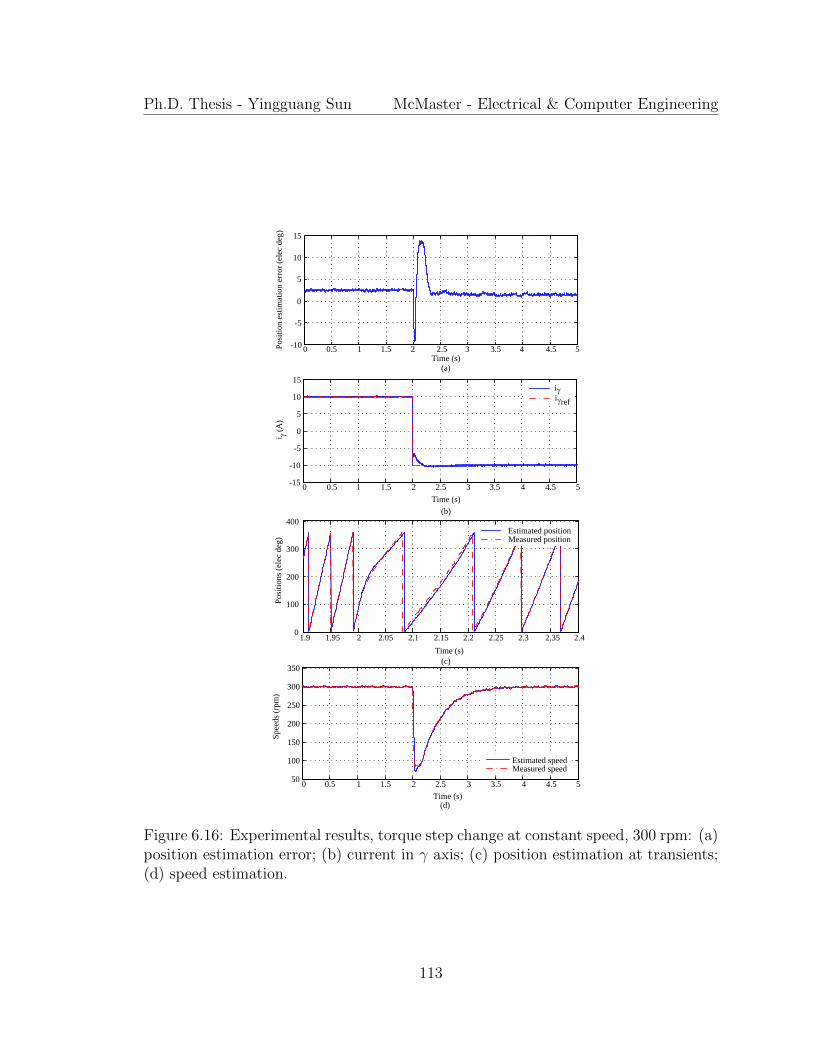
Ph.D. Thesis - Yingguang Sun McMaster - Electrical & Computer Engineering
0 0.5 1 1.5 2 2.5 3 3.5 4 4.5 5-10
-5
0
5
10
15
Time (s)
Posi
tion e
stim
atio
n e
rror
(ele
c deg
)
0 0.5 1 1.5 2 2.5 3 3.5 4 4.5 5-15
-10
-5
0
5
10
15
Time (s)
i (
A)
ii
ref
(a)
(b)
1.9 1.95 2 2.05 2.1 2.15 2.2 2.25 2.3 2.35 2.40
100
200
300
400
Time (s)
Posi
tions
(ele
c deg
)
Estimated positionMeasured position
(c)
0 0.5 1 1.5 2 2.5 3 3.5 4 4.5 550
100
150
200
250
300
350
Time (s)
Spee
ds
(rpm
)
Estimated speedMeasured speed
(d)
Figure 6.16: Experimental results, torque step change at constant speed, 300 rpm: (a)position estimation error; (b) current in γ axis; (c) position estimation at transients;(d) speed estimation.
113

Ph.D. Thesis - Yingguang Sun McMaster - Electrical & Computer Engineering
(b)
(a)
0 5 10 15 20 25
-30
-20
-10
0
10
20
30
Time (s)
Po
siti
on
est
imat
ion
err
or
(ele
c d
eg)
0 5 10 15 20 25-800
-600
-400
-200
0
200
400
600
800
Time (s)
Sp
eed
s (r
pm
)
Estimated speedMeasured speed
Figure 6.17: Experimental results, wide speed range operation: (a) position estima-tion error; (b) speed estimation.
6.7 Parameter Sensitivity Analysis
In order to better evaluate the robustness of the proposed estimation method, the
sensitivity of the motor parameters is analyzed with contour plots in Figure 6.19 and
experimental testing results in Figure 6.20. In Figure 6.19, the position estimation
errors are analyzed with 50% resistance variation, 50% permanent magnet flux vari-
ation and 50% inductance variation (saliency ratio is kept constant) assuming the
motor is running at 300 rpm with 40% rated torque. The position estimation errors
under those parameter variations are 0, 0 and 5.7 respectively. In the experimental
tests shown in Figure 6.20, the motor was running at 300 rpm and the electromagnetic
torque changed from 40% rated torque to −40% rated torque. The position estima-
tion errors due to 50% resistance variation, 50% permanent magnet flux variation and
50% inductance variation with 40% rated torque are 1.5, 0.5 and 8.5. Under the
114

Ph.D. Thesis - Yingguang Sun McMaster - Electrical & Computer Engineering
Initial position
estimation at startup
and standstill100 rpm, no load
31.5
500 rpm, no load 500 rpm, 76% rated torque
2 1
160
0 5 10 15-50
0
50
100
150
200
Time (s)
Po
siti
on
est
imat
ion
err
or
(ele
c d
eg)
(a)
0 0.5 1 1.5 2 2.5 3 3.50
100
200
300
400
Time (s)
Po
siti
on
s (e
lec
deg
)
Estimated positionMeasured position
6.2 6.25 6.3 6.35 6.4 6.45 6.5
(b)
0 5 10 15-5
0
5
10
15
Time (s)
i (
A)
i
i ref
(c)
0 5 10 15-100
0
100
200
300
400
500
600
700
Time (s)
Sp
eed
s (r
pm
)
Estimated speedMeasured speed
(d)
11.3 11.35 11.4 11.45 11.5
Figure 6.18: Experimental results, speed and position estimation at wide speed rangeincluding standstill: (a) position estimation error; (b) position estimation at tran-sients; (c) current in γ axis; (d) speed estimation.
115

Ph.D. Thesis - Yingguang Sun McMaster - Electrical & Computer Engineering
(5.7, 0)
Position error (elec deg)
Spee
d e
rror
(rpm
)
0 50 100 150 200 250 300
-300
-200
-100
0
100
200
300
Position error (elec deg)
Spee
d e
rror
(rpm
)
0 50 100 150 200 250 300
-300
-200
-100
0
100
200
300
(a)
(0, 0)
Position error (elec deg)
Spee
d e
rror
(rpm
)
0 50 100 150 200 250 300
-300
-200
-100
0
100
200
300
(0, 0)
(b)
(c)
Figure 6.19: Parameter sensitivity contour plot analysis at 300 rpm with 40% ratedtorque: (a) 50% resistance variation; (b) 50% permanent magnet flux variation; (c)50% d-q axes inductances variation.
116

Ph.D. Thesis - Yingguang Sun McMaster - Electrical & Computer Engineering
0 0.5 1 1.5 2 2.5 3 3.5 4 4.5 5-10
-5
0
5
10
15
Time (s)
Po
siti
on
est
imat
ion
err
ors
(el
ec d
eg)
-50% variation0% variation50% variation
0 0.5 1 1.5 2 2.5 3 3.5 4 4.5 5-40
-20
0
20
40
60
Time (s)
Po
siti
on
est
imat
ion
err
ors
(el
ec d
eg)
-50% variation
0% variation50% variation
(a)
(c)
0 0.5 1 1.5 2 2.5 3 3.5 4 4.5 5-10
-5
0
5
10
15
20
Time (s)
Po
siti
on
est
imat
ion
err
ors
(el
ec d
eg)
-50% variation0% variation50% variation
(b)
40% rated torque
-40% rated torque
40% rated torque
-40% rated torque
-40% rated torque
40% rated torque
Figure 6.20: Parameter sensitivity experimental test results: (a) ±50% resistancevariation; (b) ±50% PM flux variation; (c) ±50% d-q axes inductances variation.
same test condition, the position estimation errors observed in experiment are larger
than those in the theoretical contour plot analysis due to the measurement noise and
model mismatch. Besides the 300 rpm and 40% rated torque test condition with 50%
parameter variations, the results shown in Figure 6.20 also illustrate the performance
of the proposed method at torque transients, −40% rated torque condition and −50%
parameter variations. From the results, it is clear that the position estimation errors
during the torque transients are larger with ±50% parameter variations than with the
117

Ph.D. Thesis - Yingguang Sun McMaster - Electrical & Computer Engineering
original values. Regarding the steady state estimation accuracy, the proposed estima-
tion method is less affected by the resistance and permanent magnet flux variations.
However, the steady state position estimation errors change by around 7 electrical
degree with ±50% inductance variations (Sun et al., 2016).
6.8 Conclusions
In this chapter, the feasibility of a novel unified nonlinear optimization based speed
and position estimation algorithm has been proposed. A cost function is defined
based on the voltage equations in the stationary reference frame and the speed and
position information can be obtained by minimizing the cost function. At low speed,
the cost function is modified and extra high frequency voltage is injected to prevent
the singularity at zero speed. Since the position estimator structure remains the
same from standstill condition to high speed, a unified speed and position estimator
is proposed for the IPM motor drives at wide speed range. The effectiveness of the
cost functions has been validated with contour plot analysis and convexity analysis.
The real time implementation of the proposed observer has been introduced and
the feasibility of the proposed method has been validated with the prototype IPM
motor drive system. The convergence range, performance with different speed and
torque transients and the parameter sensitivity analysis have been presented in this
chapter. The experimental results demonstrate that the proposed method is capable
of estimating the speed and position robustly with high accuracy and fast convergence
at wide speed range.
118

Chapter 7
Comparative Assessment of the
Proposed Sensorless Approach
7.1 Introduction
In pulsating sinusoidal voltage injection (PSVI) based method, the speed and po-
sition estimator relies on the BPF, LPF and PLL, which have limited bandwidths
respectively. Moreover, the calculation of extended EMF also relies on the previous
estimation information in the extended EMF (EEMF) based method. However, each
estimation is an independent process in the proposed unified nonlinear optimization
(UNOP) based method. Even though the previous estimation information is needed,
it just provides the starting point for the optimization but is not involved in the real
estimation process at medium and high speed. In the benchmark reference methods,
the inputs of the PLL are position estimation errors f(θ). The PLL structure used
in the PSVI method and EEMF method in the prototype drive system is modified in
Figure 7.1. In the UNOP method, the inputs are the estimated speed and position
119

Ph.D. Thesis - Yingguang Sun McMaster - Electrical & Computer Engineering
PI
PLL
1/z
Discrete
integrator
gain
++
Filter
( )f
Figure 7.1: The modified PLL used in PSVI and EEMF methods.
instead and the PLL is working as a filter instead of being part of the position estima-
tion. In this way, the transient behavior is faster with the proposed method since it is
equivalent to open loop estimation. In order to validate this point, the performance
of the proposed unified sensorless method is compared with benchmark reference
methods at wide speed range including standstill condition in this chapter. The com-
parisons were undertaken under same test conditions and with the same experimental
test bench. Additionally, the proposed cost functions are capable of involving machine
nonlinearity, dealing with multiple voltage injection types and achieving estimation
with low sampling frequency, which is also validated in this chapter. At last, the
computational burden of the proposed method is compared with the benchmark ref-
erence methods for validating its availability of real time implementation with general
micro-controllers.
7.2 Improvements in Initial Position Estimation
In this section, the proposed initial position estimation and polarity detection meth-
ods are compared with the conventional estimation methods. The capability of involv-
ing nonlinear motor parameters in the proposed initial position estimation method is
120

Ph.D. Thesis - Yingguang Sun McMaster - Electrical & Computer Engineering
0 0.1 0.2 0.3 0.4 0.5 0.6 0.7 0.8 0.9 1-10
0
10
20
30
40
Time (s)
Po
siti
on
est
imat
ion
err
ors
(ele
c d
eg)
PSVI
UNOP
Figure 7.2: Experimental comparison on convergence speed between PSVI methodand UNOP method.
also introduced.
7.2.1 Dynamic Performance in Initial Position Estimation
In this test, the proposed estimator and the demodulation based estimator used in
PSVI method both started from the same initial position error, which was 30 elec-
trical degree. The injected voltage magnitude, the injection frequency and the PLL
parameters are identical in the two methods. The position estimation errors are
shown in Figure 7.2. The 2% settling time and the 10%-90% rise time of the PSVI
method are 0.4 s and 0.07 s. While in UNOP method they are only 0.18 s and 0.03 s
respectively.
Figure 7.3 depicts the position estimation performances of the UNOP method and
the PSVI method during torque transients. In Figure 7.3 (a), the iγ was controlled to
generate 20% rated torque. The steady state position estimation errors are similar in
the two methods. However, the PSVI method has a much worse dynamic performance
with maximum 22 error and 2 s settling time in Figure 7.3 (a). The similar situation
is also obtained in Figure 7.3 (b) when 40% rated torque was applied. The above
121

Ph.D. Thesis - Yingguang Sun McMaster - Electrical & Computer Engineering
tests demonstrate that the proposed position estimator has faster dynamic estimation
performance than the demodulation based estimator at standstill. The BPF and LPF
in the PSVI method limit the bandwidth of demodulation based position estimator.
0 1 2 3 4 5 6-20
-10
0
10
20
30
Time (s)
Po
siti
on
est
imat
ion
err
ors
(ele
c d
eg)
PSVI
UNOP
(a)
0 1 2 3 4 5 6-40
-20
0
20
40
60
Time (s)
Po
siti
on
est
imat
ion
err
ors
(ele
c d
eg)
PSVI
UNOP
No load 20% rate torque
No load 40% rate torque
(b)
Figure 7.3: Experimental comparison on torque transient performance between PSVImethod and UNOP method: (a) 20% rated torque change; (b) 40% rated torquechange.
7.2.2 Magnetic Polarity Detection
As stated in Section 3.5.2, the conventional dual voltage injection (DVI) based polar-
ity detection method relies on the detection of the current peak difference induced by
the positive and negative voltage pulses. This method was also implemented in the
prototype motor drives. Figure 7.4 depicts the required resulting currents for robustly
detecting the polarity with the proposed method and the DVI method. The injection
duration of each voltage vector is 4Ts in the proposed method and is 6Ts in the DVI
122

Ph.D. Thesis - Yingguang Sun McMaster - Electrical & Computer Engineering
Res
ult
ing
a
xis
cu
rren
ts o
f p
ola
rity
det
ecti
on
(A
)
0 5 10 15 20 25 30-10
-5
0
5
10
Current samples
4Ts
6Ts
5.8 A
-5.5 A
9.2 A
-8.4 A
Figure 7.4: Resulting δ axis currents due to the injection in magnetic polarity detec-tion.
method. In the proposed method, the current difference between the positive peak
and negative peak is only 0.3 A. The DVI method couldn’t work robustly with this
current difference level due to its sensitivity to the measurement noise. The current
peak difference becomes larger when the injection duration increases to 6Ts, with
which the DVI method can detect the polarity reliably. However, 0.8 A difference is
still not significant enough for many drive systems with larger measurement noise. In
order to obtain significant current peak difference, the resulting currents need to be
further increased by increasing the injected voltage magnitude or injection duration,
which leads to the utilization of higher power rating inverters. Instead of only taking
the peak currents in the red squares into account, the proposed polarity detection
method involves more current samples (green bubbles), which concern the shape of
the current responses. Since the shape of the resulting currents reflects the nonlinear
properties of the machine, the proposed polarity detection method can detect the
polarity with lower currents and the robustness is enhanced compared with the DVI
method.
123

Ph.D. Thesis - Yingguang Sun McMaster - Electrical & Computer Engineering
-400 -300 -200 -100 0 100 200 300 4000
10
20
30
40
50
60
Position estimation error (elec deg)
Cost
0
60
120
180
240
300
360180 180
Figure 7.5: Plot of Gi(θ) versus position estimation errors at different initial positionsfor m = 1 using experimental data.
7.2.3 Involvement of Machine Nonlinearity in Initial Position
Estimation
In Section 4.3, the flux linkage profiles in d-q axes were measured from experiment.
The derived nonlinear inductance profiles in (4.3) can also be used in initial position
estimation. If the constant Ldq are replaced by those nonlinear inductance profiles,
the cost function (5.5) is rewritten as
minimizeθ
Gi(θ) =m∑k=1
∥∥∥Tdq(θ)uαβ(k) (7.1)
− 1
Ts∇idq`dq
(Tdq(θ)iαβ(k + 1)
)Tdq(θ)
(iαβ(k + 1)− iαβ(k)
)∥∥∥2.A similar plot of the cost function (7.1) as Figure 5.5 is shown in Figure 7.5. With
nonlinear inductance profiles involved, the cost function also has two local minimums
which locate around 0 error and 180 error in one electrical period. The initial
position can be estimated by the line search approach utilized in Chapter 5. Even
124

Ph.D. Thesis - Yingguang Sun McMaster - Electrical & Computer Engineering
though the costs are smaller at 0 error than those at 180 error, the difference is
not significant if the measurement noises are taken into account in the real time
implementation. Hence, the magnetic polarity detection is still necessary if (7.1) is
employed for position estimation in Step I. Moreover, the nonlinear inductance profiles
are not used in Step III in initial position estimation and running state estimation due
to the increased computation burden caused by the interpolation of look-up tables in
the real time implementation with 10 KHz sampling frequency.
As stated in Chapter 5, the maximum magnitude of the injected voltages for
both position estimation and polarity detection was 200 V due to the restriction
of the DC link voltage. When the magnitude of the injection voltage is fixed, the
injection duration can be adjusted to achieve higher resulting currents. The position
estimation accuracy by linear method (using constant parameters in cost function
(5.5)) and nonlinear method (using nonlinear inductance profiles in cost function
(7.1)) were tested when m ∈ [3 5] at different initial positions in one electrical period.
The results are shown in Figure 7.6 and Figure 7.7. From the comparison of the two
figures, it is clear to see that the position estimation accuracy improves as the increase
of the injection duration. The improvement of the estimation accuracy with the linear
method is not as significant as the accuracy improvement with the nonlinear method.
Additionally, estimation accuracies of the linear and nonlinear methods are also
compared with the same injection duration (5Ts) in Figure 7.8. In the figure, the peak
error and average error in the nonlinear method are 15 and 7.15 respectively. Both
the peak error and average error in the linear method are larger, which are 28.8 and
10.77. Moreover, the estimation accuracies of the nonlinear method are also higher
than those of linear method with other injection durations (3Ts and 4Ts), which are
125

Ph.D. Thesis - Yingguang Sun McMaster - Electrical & Computer Engineering
0 50 100 150 200 250 300-40
-30
-20
-10
0
10
20
30
Initial positions (elec deg)
Est
imat
ion
err
ors
(el
ec d
eg)
5Ts4Ts3Ts
330
Figure 7.6: Position estimation errors of the linear method at different initial positionswith different injection durations.
summarized in Table 7.1.
The nonlinear method mentioned in this section can be used for initial position
estimation in Step I when the nonlinear flux linkage profiles are available. So this
method is heavier parameter dependent and needs more computation source com-
pared with the linear method. Moreover, even though the estimation accuracy is
improved by involving machine nonlinearities, the estimation accuracy is still large
compared with the accuracy after Step III in Chapter 5 due to the inverter nonlin-
earity. So the linear method is chosen as the proposed initial position estimation
Table 7.1: Position Estimation Accuracy Comparison
Injection durations foreach voltage vector (ms)
0.3 0.4 0.5
Average estimation errorof linear method (elec deg)
13.14 11.92 10.77
Average estimation errorof nonlinear method (elec deg)
12.5 10.27 7.15
Peak value of currentpulse in per unit value
0.39 0.52 0.69
126

Ph.D. Thesis - Yingguang Sun McMaster - Electrical & Computer Engineering
0 50 100 150 200 250 300-30
-20
-10
0
10
20
30
Initial positions (elec deg)
Est
imat
ion e
rrors
(el
ec d
eg)
5Ts4Ts3Ts
330
Figure 7.7: Position estimation errors of the nonlinear method at different initialpositions with different injection durations.
method in this thesis. However, the nonlinear method still demonstrates its capabil-
ity of involving nonlinear motor parameters in the cost functions for improving the
estimation accuracy.
7.3 Improvements in Speed and Position Estima-
tion at Running State
7.3.1 Dynamic Performance at Low Speed
In order to benchmark the proposed speed and position estimation algorithm at low
speed, the same test in Figure 6.14 was duplicated by the PVSI method. The band-
width of the PLL used in PSVI method was tuned to be 36 times larger than that of
the PLL used in proposed position estimator, in order to achieve similar bandwidths
with the proposed method in speed and current responses. The variable magnitude
127

Ph.D. Thesis - Yingguang Sun McMaster - Electrical & Computer Engineering
0 50 100 150 200 250 300-30
-20
-10
0
10
20
30
Initial positions (elec deg)
Est
imat
ion
err
or
(ele
c d
eg)
Nonlinear Method
Linear Method
330
Figure 7.8: Estimation accuracy comparison between nonlinear and linear methods(5Ts for each voltage pulse).
injection method can’t be applied to the PSVI method due to the fact that the es-
timation solely relies on the injection frequency components. Reducing the injection
voltage magnitude will affect the estimation since the carrier frequency current re-
duces accordingly. However, both the fundamental frequency components and carrier
frequency components are utilized for estimation in the proposed method, so the
injection voltage can be reduced as the motor speed increases. Hence, the injected
voltage magnitude has to be kept constant at 70 V in the PSVI method at low speed.
For the testing results of the PSVI method in Figure 7.9 (a), the 2% settling times of
the speed step change from 0 to 50 rpm and from 50 rpm to negative -50 rpm are 4.3
s and 5.6 s respectively. While in the UNOP method, the settling times are only 0.1 s
and 0.15 s shown in Figure 6.14 (a). The settling times of the UNOP method are 40
times shorter than those of the PSVI method. The comparison also shows that the
UNOP method has lower transient and steady state position estimation error. The
maximum transient error is −26 with PSVI method and is −16 with the UNOP
method. The estimated speed ripple is smaller with the UNOP method (10 rpm peak
128

Ph.D. Thesis - Yingguang Sun McMaster - Electrical & Computer Engineering
0 5 10 15 20 25-30
-25
-20
-15
-10
-5
0
Time (s)
Posi
tion e
stim
atio
n e
rror
(ele
c deg
)
(a)
2 2.5 3 3.5 40
50
100
150
200
250
300
350
400
Time (s)
Posi
tions
(ele
c deg
)
Estimated position
Measured position
14 14.2 14.4 14.6 14.8 15
Time (s)
(b)
0 5 10 15 20 25-80
-60
-40
-20
0
20
40
60
80
Time (s)
Spee
ds
(rpm
)
Estimated speedMeasured speed
(c)
Figure 7.9: Benchmark reference, speed and position estimation with PSVI methodwith the same test shown in Figure 6.14: (a) position estimation error; (b) positionestimation at transients; (c) speed estimation.
to peak) than that with the PSVI method (30 rpm peak to peak), which is illustrated
in Figure 6.14 (c) and Figure 7.9 (c). Hence, it can be concluded that the UNOP
method outperforms the PSVI method that uses demodulation for speed and position
sensing at low speed.
Besides the speed transients, the estimation performance of the UNOP method
and PSVI method were also compared in the torque transient tests and the results
are illustrated in Figure 7.10 and Figure 7.11. In this test, the motor was running
129

Ph.D. Thesis - Yingguang Sun McMaster - Electrical & Computer Engineering
0 0.5 1 1.5 2 2.5 3 3.5 4 4.5 5-10
-5
0
5
10
15
20
25
Time (s)
Posi
tion e
stim
atio
n e
rror
(ele
c deg
)
1.6 1.8 2 2.2 2.4 2.6 2.8 30
100
200
300
400
Time (s)
Posi
tions
(ele
c deg
)
Estimated positionMeasured position
(a)
(b)
0 0.5 1 1.5 2 2.5 3 3.5 4 4.5 5-5
-4
-3
-2
-1
0
1
2
3
4
5
Time (s)
i
(A)
(c)
0 0.5 1 1.5 2 2.5 3 3.5 4 4.5 50
50
100
150
Time (s)
Spee
ds
(rpm
)
Estimated speedMeasured speed
(d)
iref
i
Figure 7.10: Experimental results of the UNOP method at low speed, torque stepchange at 100 rpm: (a) position estimation error; (b) position estimation at transients;(c) current in γ axis (d) speed estimation.
130

Ph.D. Thesis - Yingguang Sun McMaster - Electrical & Computer Engineering
0 0.5 1 1.5 2 2.5 3 3.5 4 4.5 5-10
-5
0
5
10
15
20
25
Time (s)
Post
itio
n e
stim
atio
n e
rror
(ele
c deg
)
1.6 1.8 2 2.2 2.4 2.6 2.8 30
50
100
150
200
250
300
350
400
Time (s)
Posi
tions
(ele
c deg
)
Estimated positionMeasured position
(a)
(b)
0 0.5 1 1.5 2 2.5 3 3.5 4 4.5 5-5
-4
-3
-2
-1
0
1
2
3
4
5
Time (s)
i
(A)
iiref
(c)
0 0.5 1 1.5 2 2.5 3 3.5 4 4.5 50
50
100
150
Time (s)
Spee
ds
(rpm
)
Estimated speed
Measured speed
(d)
Figure 7.11: Benchmark reference, PSVI base method at low speed, torque stepchange at 100 rpm: (a) position estimation error; (b) position estimation at transients;(c) current in γ axis; (d) speed estimation.
131
Ph.D. Thesis - Yingguang Sun McMaster - Electrical & Computer Engineering
at 100 rpm and the electromagnetic torque was controlled to change from 30% rated
torque to −30% rated torque. The similar tracking performance is obtained in the
current and speed transients in Figure 7.10 and Figure 7.11. However, the larger
position estimation ripple, the larger steady state position estimation error and the
larger estimated speed ripple are obtained in the PSVI method.
7.3.2 Dynamic Performance at High Speed
At high speed, the estimation performance of the proposed method is compared with
the EEMF method. The bandwidth of the PLL used in EEMF method was tuned
to be 22 times larger than that of the PLL used in proposed position estimator, in
order to achieve similar bandwidths with the proposed method in speed and current
responses. Figure 7.12 and Figure 7.13 illustrate the experimental results when the
motor speed increased from 400 rpm to 600 rpm with 15% rated torque. The 2%
settling times for the EEMF method and the UNOP method are 5 s and 0.7 s respec-
tively. The settling time of the proposed method is 7.1 times shorter than that of the
benchmark reference in this test. The maximum transient position estimation error
is 8.7 in the EEMF method and is only 2.4 in the UNOP method.
Figure 7.14 and Figure 7.15 depict the experimental results when the torque
changed from 30% rated torque to −30% rated torque at 400 rpm. The 2% settling
times for the EEMF method and the UNOP method are 1s and 1.2 s respectively. The
maximum transient position estimation error is −4.5 in the EEMF based method
and is 10 in the UNOP method. In this test, the transient error is larger in the
UNOP method. However, the ripples of the estimated speed and position are much
larger in EEMF method than those in the proposed method. Moreover, the UNOP
132

Ph.D. Thesis - Yingguang Sun McMaster - Electrical & Computer Engineering
0 2 4 6 8 10 12-2
0
2
4
6
8
10
Time (s)
Posi
tion e
stim
atio
n e
rror
(ele
c deg
)
2.8 2.85 2.9 2.95 3 3.050
100
200
300
400
Time (s)
Posi
tions
(ele
c deg
)
Estimated position
Measured position
(a)
(b)
0 2 4 6 8 10 120
0.5
1
1.5
2
2.5
Time (s)
i
(A)
i
i
ref
(c)
0 2 4 6 8 10 12350
400
450
500
550
600
650
Time (s)
Spee
ds
(rpm
)
Estimated speed
Measured speed
(d)
Figure 7.12: Benchmark reference, EEMF base method at high speed, speed stepchange with 15% rated torque: (a) position estimation error; (b) position estimationat transients; (c) current in γ axis; (d) speed estimation.
133

Ph.D. Thesis - Yingguang Sun McMaster - Electrical & Computer Engineering
(a)
0 2 4 6 8 10 120
0.5
1
1.5
2
2.5
Time (s)
i
(A)
ii
ref
0 2 4 6 8 10 12-2
0
2
4
6
8
10
Time (s)
Po
siti
on
est
imat
ion
err
or
(ele
c d
eg)
2.8 2.85 2.9 2.95 3 3.050
100
200
300
400
Time (s)
Po
siti
on
s (e
lec
deg
)
Estimated position
Measured position
0 2 4 6 8 10 12350
400
450
500
550
600
650
Time (s)
Sp
eed
s (r
pm
)
Estimated speed
Measured speed
(b)
(c)
(d)
3.1
Figure 7.13: Experimental results of the UNOP method at high speed, speed stepchange with 15% of rated torque: (a) position estimation error; (b) position estimationat transients; (c) current in γ axis; (d) speed estimation.
134

Ph.D. Thesis - Yingguang Sun McMaster - Electrical & Computer Engineering
0 2 4 6 8 10 12-6
-4
-2
0
2
4
6
8
Time (s)
Posi
tion e
stim
atio
n e
rror
(ele
c deg
)
0 2 4 6 8 10 12-5
0
5
Time (s)
i
(A)
i
i ref
(a)
(c)
2.95 2.96 2.97 2.98 2.99 3 3.01 3.02 3.03 3.04 3.050
50
100
150
200
250
300
350
400
Time (s)
Posi
tions
(ele
c deg
)
Estimated position
Measured position
(b)
0 2 4 6 8 10 12300
320
340
360
380
400
420
Time (s)
Spee
ds
(rpm
)
Estimated speed
Measured speed
(d)
Figure 7.14: Benchmark reference, EEMF base method at high speed, torque stepchange at 400 rpm: (a) position estimation error; (b) position estimation at transients;(c) current in γ axis; (d) speed estimation.
135

Ph.D. Thesis - Yingguang Sun McMaster - Electrical & Computer Engineering
0 2 4 6 8 10 12-6
-4
-2
0
2
4
6
8
10
12
Time (s)
Posi
tion e
stim
atio
n e
rrors
(ele
c deg
)
(a)
2.95 2.96 2.97 2.98 2.99 3 3.01 3.02 3.03 3.04 3.050
50
100
150
200
250
300
350
400
Time (s)
Posi
tions
(ele
c deg
)
Estimated position
Measured position
(b)
0 2 4 6 81
0
1
2
-5
0
5
Time (s)
i (
A)
i
i
ref
0 2 4 6 8 10 12300
320
340
360
380
400
420
Time (s)
Spee
ds
(rpm
)
Estimated position
Measured position
(c)
(d)
Figure 7.15: Experimental results of the UNOP method at high speed, torque stepchange at 400 rpm: (a) position estimation error; (b) position estimation at transients;(c) current in γ axis; (d) speed estimation.
136

Ph.D. Thesis - Yingguang Sun McMaster - Electrical & Computer Engineering
method is more reliable with larger torque step change. For example, the same test
shown in Figure 6.16 was also implemented with the EEMF method. However, the
estimation failed due to the divergence of the estimator during the torque transients.
7.3.3 Switch Between Low Speed and High Speed
0 2 4 6 8 10 12 14-15
-10
-5
0
5
10
15
20
Time (s)
Posi
tion e
stim
atio
n e
rror
(ele
c deg
)
(a)
2.4 2.45 2.5 2.55 2.6 2.65 2.7 2.75 2.80
100
200
300
400
Time (s)
Posi
tions
(ele
c deg
)
Estimated position
Measured position
7.8 7.85 7.9 7.95 8 8.05 8.1 8.15 8.2 8.25 8.3
(b)
0 2 4 6 8 10 12 1450
100
150
200
250
300
350
Time (s)
Spee
ds
(rpm
)
Estimated speed
Measured speed
(c)
Figure 7.16: Benchmark reference, the combined method during switch process, speedstep change without load: (a) position estimation error; (b) position estimation attransients; (c) speed estimation.
In Section 3.4, the wide speed range sensorless method which combines low speed
137

Ph.D. Thesis - Yingguang Sun McMaster - Electrical & Computer Engineering
0 2 4 6 8 10 12-15
-10
-5
0
5
10
15
20
Time (s)
Posi
tion e
stim
atio
n e
rror
(ele
c deg
)
(a)
2.9 2.95 3 3.05 3.1 3.15 3.20
100
200
300
400
Time (s)
Posi
tions
(ele
c deg
)
Estimated speed
Measured speed
7.3 7.35 7.4 7.45 7.5 7.55 7.6
(b)
0 2 4 6 8 10 12250
300
350
400
450
500
550
Time (s)
Spee
ds
(rpm
)
Estimated speed
Measured speed
(c)
Figure 7.17: Experimental results of the proposed unified method during switch pro-cess, speed step change without load: (a) position estimation error; (b) positionestimation at transients; (c) speed estimation.
and high speed estimation algorithms was introduced. In the sensorless control sys-
tem shown in Figure 3.6, there are two position estimators and two PLLs with differ-
ent parameters. While in the proposed sensorless control system, only one position
estimator is needed. As mentioned in Section 7.3.1, the variable magnitudes high fre-
quency voltage injection can not be applied to the PSVI method. Hence, the choice
of the switch speed is different in the reference combined method and the proposed
UNOP method. The N1 and N2 were selected as 150 rpm and 190 rpm in the reference
138

Ph.D. Thesis - Yingguang Sun McMaster - Electrical & Computer Engineering
0 2 4 6 8 10 12-25
-20
-15
-10
-5
0
5
10
15
Time (s)
Posi
tion e
stim
atio
n e
rror
(ele
c deg
)
0 2 4 6 8 10 122
3
4
5
6
Time (s)
i (
A)
i
i ref
(a)
(b)
0 2 4 6 8 10 1250
100
150
200
250
300
350
Time (s)
Spee
ds
(rpm
)
Estimated speed
Measured speed
(c)
Figure 7.18: Benchmark reference, the combined method during switch process, speedstep change with 30% rated torque: (a) position estimation error; (b) current in γaxis; (c) speed estimation.
combined method while the N1 in the proposed UNOP method was 400 rpm. Figure
7.16 to Figure 7.19 show the experimental results of the reference combined method
and the proposed UNOP method during the switch process with 0% torque and 30%
rated torque. The proposed method outperforms at faster dynamic response speed,
lower average steady state position estimation error and lower maximum transient
position estimation error. Moreover, the sensorless control system is greatly simpli-
fied by employing only one unified method from standstill condition to high speed
139

Ph.D. Thesis - Yingguang Sun McMaster - Electrical & Computer Engineering
0 1 2 3 4 5 6 7 8 9 10-25
-20
-15
-10
-5
0
5
10
15
Time (s)
Po
siti
on
est
imat
ion
err
or
(ele
c d
eg)
0 1 2 3 4 5 6 7 8 9 102
3
4
5
6
Time (s)
i (
A)
i
i ref
0 1 2 3 4 5 6 7 8 9 10250
300
350
400
450
500
550
Time (s)
Sp
eed
s (r
pm
)
Estimated speed
Measured speed
(a)
(b)
(c)
Figure 7.19: Experimental results of the proposed unified method during switch pro-cess, speed step change with 30% rated torque: (a) position estimation error; (b)current in γ axis; (c) speed estimation.
operation instead of utilizing two different position estimators.
7.4 Capability of Speed and Position Estimation
with Multiple Injection Types
In Step III of initial position estimation, the proposed optimization based method
is capable with sinusoidal injection as well as other injection types, i.e. rectangular
voltages. In (Kondo et al., 1995; Jeong et al., 2005; Bolognani et al., 2011; Aihara
140

Ph.D. Thesis - Yingguang Sun McMaster - Electrical & Computer Engineering
Step I
aV
aI
5 sT 10 sT 5 sT
Step II
4 sT 8 sT 4 sT
Step III
2ms
Figure 7.20: Screenshot of the scope, continuous rectangular voltage injection in StepIII.
et al., 1999; Foo et al., 2010; Gong and Zhu, 2013; Kim et al., 2012; Yoon et al., 2011;
Murakami et al., 2012; Park and Kim, 2014; Zaim et al., 2014; Huang et al., 2014),
the demodulation methods for sinusoidal injection and rectangular injection were dif-
ferent. However, a unified position estimation algorithm for different voltage injection
types is achieved by using the proposed optimization based estimator. Figure 7.20
illustrates the screenshot of scope when continuous rectangular voltage was injected
in Step III. The initial position estimation performances are similar in Figure 5.13
with sinusoidal injection and Figure 7.21 with rectangular injection.
Besides the initial position estimation, the rectangular voltage injection can also
be employed at wide speed range operations as shown in Figure 7.22. In Figure 7.22
(a), the actual initial position was -178. After the initial position estimation, the
steady state estimation error is 2. The machine speed increased to 100 rpm and
then to 500 rpm. The 76% rated torque was applied to the machine shaft when the
motor was running at 500 rpm. The steady state position estimation error is less
than 2 and the maximum transient position estimation error is less than 20. Figure
141

Ph.D. Thesis - Yingguang Sun McMaster - Electrical & Computer Engineering
0 0.05 0.1 0.15 0.2 0.25 0.3 0.35 0.40
10
20
30
40
50
Time (s)
Po
siti
on
s (e
lec
deg
)
Estimated position
Measured position
0 0.05 0.1 0.15 0.2 0.25 0.3 0.35 0.4
0
10
20
30
40
Time (s)
Po
siti
on
est
imat
ion
err
or
(ele
c d
eg)
Step I and II,
4.1ms in total
Step III, keep
estimating at
standstill
1.9
41.5
(a)
(b)
Figure 7.21: Experimental results on initial position estimation at 41.5 with rectan-gular voltage injection: (a) measured and estimated positions; (b) position estimationerror.
7.22 (b), (c) and (d) illustrates the position estimation at transients, iγ and speed
estimation respectively. The proposed sensorless control method proves to be valid
with rectangular voltage injection at wide speed range.
7.5 Capability of Speed and Position Estimation
with Low Sampling Frequency
Estimating speed and position with low sampling frequency is attractive for high
power AC motor drives, which is challenging for the signal injection based estima-
tion methods at low speed. These methods rely on the demodulation of the carrier
142

Ph.D. Thesis - Yingguang Sun McMaster - Electrical & Computer Engineering
0 5 10 15-200
-150
-100
-50
0
50
Time (s)
Po
siti
on
est
imat
ion
err
or
(ele
c d
eg)
178
Initial position
estimation at startup
and standstill
100 rpm, no load
22
500 rpm, no load 500 rpm, 76%
rated torque
2 1
(a)
0 1 2 3 40
100
200
300
400
Time (s)
Po
siti
on
s (e
lec
deg
)
Estimated positionMeasured position
7 7.05 7.1 7.15 7.2 7.25 7.3
(b)
0 5 10 15-5
0
5
10
15
Time (s)
i (
A)
i
i ref
0 5 10 15-100
0
100
200
300
400
500
600
700
Time (s)
Sp
eed
s (r
pm
)
Estimated speed
Measured speed
(c)
(d)
12.3 12.35 12.4 12.45 12.5
Figure 7.22: Experimental results, speed and position estimation with continuousrectangular voltage injection: (a) position estimation error; (b) position estimationat transients; (c) current in γ axis; (d) speed estimation.
143
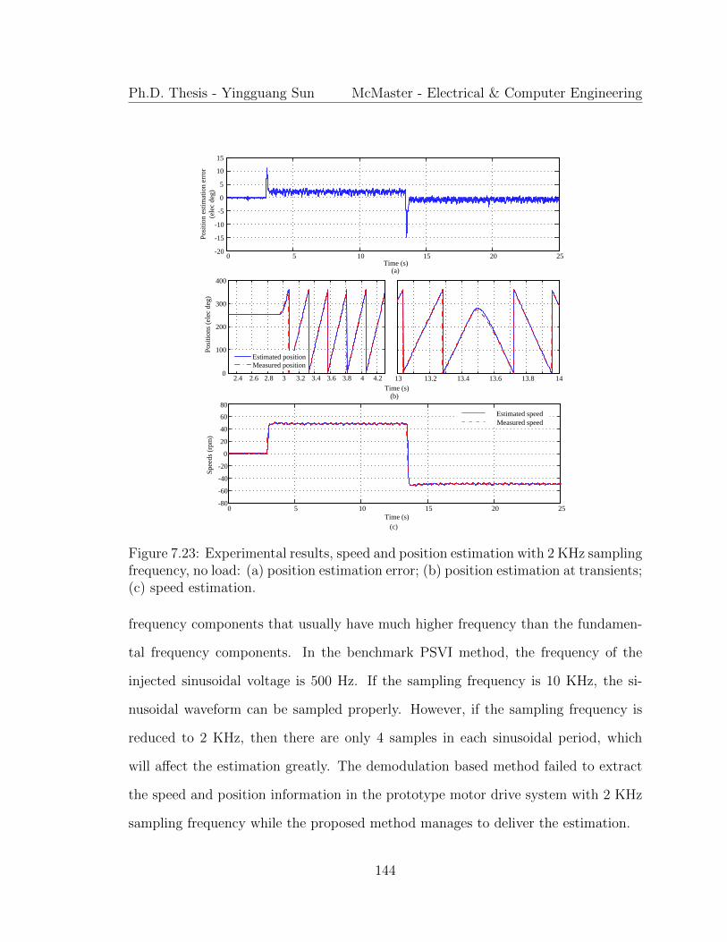
Ph.D. Thesis - Yingguang Sun McMaster - Electrical & Computer Engineering
(a)
Time (s)
(b)
Time (s)
(c)
0 5 10 15 20 25-20
-15
-10
-5
0
5
10
15
Time (s)
Po
siti
on
est
imat
ion
err
or
(ele
c d
eg)
2.4 2.6 2.8 3 3.2 3.4 3.6 3.8 4 4.20
100
200
300
400
Po
siti
on
s (e
lec
deg
)
Estimated position
Measured position
13 13.2 13.4 13.6 13.8 14
0 5 10 15 20 25-80
-60
-40
-20
0
20
40
60
80
Sp
eed
s (r
pm
)
Estimated speed
Measured speed
Figure 7.23: Experimental results, speed and position estimation with 2 KHz samplingfrequency, no load: (a) position estimation error; (b) position estimation at transients;(c) speed estimation.
frequency components that usually have much higher frequency than the fundamen-
tal frequency components. In the benchmark PSVI method, the frequency of the
injected sinusoidal voltage is 500 Hz. If the sampling frequency is 10 KHz, the si-
nusoidal waveform can be sampled properly. However, if the sampling frequency is
reduced to 2 KHz, then there are only 4 samples in each sinusoidal period, which
will affect the estimation greatly. The demodulation based method failed to extract
the speed and position information in the prototype motor drive system with 2 KHz
sampling frequency while the proposed method manages to deliver the estimation.
144

Ph.D. Thesis - Yingguang Sun McMaster - Electrical & Computer Engineering
Time (s)
(a)
(b)
(c)
0 5 10 15 20 25-30
-25
-20
-15
-10
-5
0
5
Time (s)
Po
siti
on
est
imat
ion
err
or
(ele
c d
eg)
2.5 3 3.5 40
100
200
300
400
Estimated positionMeasured position
Po
siti
on
s (e
lec
deg
)
13 13.2 13.4 13.6 13.8 14
0 5 10 15 20 25-80
-60
-40
-20
0
20
40
60
80
Time (s)
Sp
eed
s (r
pm
)
Estimated speed
Measured speed
Figure 7.24: Experimental results, speed and position estimation with 2 KHz sam-pling frequency, with 40% rated torque: (a) position estimation error; (b) positionestimation at transients; (c) speed estimation.
Figure 7.23 and Figure 7.24 depict the speed and position estimation results of
the proposed method with 2 KHz sampling frequency. The testing conditions were
consistent with Figure 6.12 and Figure 6.14. From the comparison, it is clear that
the transient position estimation error increases with 2 KHz sampling frequency than
that with 10 KHz sampling frequency. But the steady state estimation performance is
similar in the two tested sampling frequencies. As mentioned in Section 7.2.3, involv-
ing nonlinear motor parameters at running state estimation with 10 KHz sampling
is challenging with the micro-controller used in the prototype motor drive system.
Nevertheless, reducing the sampling frequency to 2 KHz would help in utilizing the
145

Ph.D. Thesis - Yingguang Sun McMaster - Electrical & Computer Engineering
nonlinear inductance profiles in the running state speed and position estimation.
7.6 Computational Burden Analysis
The online optimization technique used in the real time implementation of the pro-
posed method was introduced in Section 6.5. A certain number of iterations are both
needed in searching the optimal coefficient ξ and the minimum cost in a certain decent
direction in Step III and running state estimation. The maximum iterations that the
MicroAutoBox II can handle with 10 KHz sampling frequency is 18 iterations and
the minimum iteration number is 1. The computational burden is reflected in the
turnaround time (TAT) of the control system. The TATs of the proposed method
with maximum and minimum iterations are 85 µs and 33 µs respectively. The TAT
of the benchmark reference method is 29 µs, which is close to the proposed method
with minimum iteration.
The performances of the UNOP method with maximum iterations and minimum
iteration were compared with the benchmark reference method at machine startup.
The injected voltage magnitude, the injection frequency and the PLL parameters are
identical in the proposed method and the benchmark reference. In Figure 7.25, the
proposed estimator and the demodulation based estimator both started from the same
initial error, which was 30 in this case. From the results, it is clear that the 10%-
90% rise time and the 2% settling time are very close with maximum and minimum
iterations in the proposed method, which are 0.03 s and 0.18 s respectively. The
similar performance with maximum and minimum iterations is due to the execution
of the online optimization in 10 KHz. The 10%-90% rise time and the 2% settling
time in the benchmark reference method are 0.07 s and 0.4 s respectively.
146

Ph.D. Thesis - Yingguang Sun McMaster - Electrical & Computer Engineering
0 0.1 0.2 0.3 0.4 0.5 0.6 0.7 0.8 0.9 1-10
0
10
20
30
40
Time (s)
Po
siti
on
est
imat
ion
err
ors
(ele
c d
eg)
Benchmark reference
UNOP with max itersUNOP with min iters
Figure 7.25: Estimation performance validation with different iterations, convergencetest with 30 initial error.
The estimation performances of the proposed method with maximum and mini-
mum iterations and the benchmark reference method during speed and torque tran-
sients are compared in Figure 7.26. The test conditions in Figure 7.26 (a) and (b)
illustrate the speed and torque transients respectively. The bandwidth of the PLL
used in the benchmark reference method is 36 times larger than that used in the
proposed method. From the comparison, it is concluded that the proposed method
with minimum iteration has similar performance with maximum iterations. More-
over, the TAT of the proposed method with minimum iteration is close to that of
the benchmark reference method. But the UNOP method outperforms the bench-
mark reference method both in dynamic response speed and steady state estimation
accuracy.
At last, the performance comparisons between the UNOP method, the EEMF
method and the PSVI method are summarized in Figure 7.27 in six perspectives,
which are convergence speed, reliability, computational burden, conceptual complex-
ity, wide speed range operation capability and low sampling frequency operation ca-
pability. The UNOP method outperforms in convergence speed, reliability, capability
of wide speed range operation and capability of low sampling frequency operation.
147

Ph.D. Thesis - Yingguang Sun McMaster - Electrical & Computer Engineering
0 5 10 15-50
-40
-30
-20
-10
0
10
Time (s)
Posi
tion e
stim
atio
n e
rrors
(el
ec d
eg)
UNOP with max itersUNOP with min itersBenchmark reference
(a)
(b)
0 rpm100 rpm
-100 rpm
0 0.5 1 1.5 2 2.5 3 3.5 4 4.5 5-10
-5
0
5
10
15
20
25
Time (s)
Posi
tion e
stim
atio
n e
rrors
(el
ec d
eg)
UNOP with max itersUNOP with min itersBenchmark reference
30% rated torque-30% rated torque
Figure 7.26: Estimation performance validation with different iterations: (a) speedtransients; (b) torque transients.
Convergence speed
Reliability
Computational
burden
Conceptual
complexity
Wide speed range
operation capability
Low sampling
frequency operation
capability
UNOP EEMF PSVI
Figure 7.27: Sensorless methods comparison.
148

Ph.D. Thesis - Yingguang Sun McMaster - Electrical & Computer Engineering
7.7 Conclusions
In this chapter, the proposed unified speed and position estimation method is com-
pared with the reference combined estimation method on the same experimental test
bench. Under the same test conditions, the proposed method outperforms with its
excellent dynamic performance and steady state accuracy. Since the proposed method
is able to employ both the fundamental frequency components and high frequency
components, the sensorless control method is unified at low speed and high speed with-
out involving two different estimators, which greatly reduces the system complexity.
Moreover, the cost functions defined in the proposed method are capable of dealing
with different voltage injection types and nonlinear motor parameters, which make
this method more flexible under different requirements. Additionally, the capability
of estimating speed and position with low sampling frequency benefits for involving
machine nonlinearity at running state estimation. At last, the computational burden
of the proposed method with maximum and minimum iterations is compared with
the benchmark reference method. The proposed method with minimum iteration has
similar TAT with the benchmark reference but outperforms both in dynamic and
steady state performance.
149

Chapter 8
Conclusions and Future Work
8.1 Conclusions
In this thesis, a unified speed and position estimation method at wide speed range
including standstill has been presented.
A novel nonlinear IPM motor model relying on the current-flux linkage profiles of
the prototype machine has been introduced in Chapter 4. The original flux-current
profiles were measured experimentally and were inverted to current-flux profiles by
employing the proposed LUTs inversion method using nonlinear optimization. This
novel model is utilized for the simulation validation of the proposed initial position
estimation method and the simulation results match with the experimental results
very well.
At machine startup and standstill, an optimization based initial position estima-
tion algorithm has been proposed. A cost function is defined and the initial position
can be estimated by searching the minimum of the cost function. Three steps which
150

Ph.D. Thesis - Yingguang Sun McMaster - Electrical & Computer Engineering
employ different voltage injections are utilized. The pulse voltage injection for posi-
tion estimation benefits from its fast response, but polarity detection and accuracy
improvements are still needed. The proposed magnetic polarity detection method
generalizes the polarity detection techniques for different IPM motor drives. The
polarity can be detected once the differential inductance profile is known. Compared
with methods relying solely on saturation, the proposed method requires lower cur-
rents to reliably determine the polarity. The continuous voltage injection is used
for position estimation at standstill condition after the initial position is roughly ob-
tained. The involvement of continuous injection in Step III improves the estimation
accuracy and proposes a unified solution for integrating the speed and position es-
timation at standstill condition and running state. The feasibility of the proposed
initial position estimation method has been investigated and validated with both
simulation and experimental tests. The initial position can be identified within 50
milliseconds and the position estimation error is less than 1 electrical degree.
At running state, a nonlinear optimization based speed and position estimation
algorithm has been presented. A cost function is defined which utilizes both speed and
position as decision variables and the speed and position information can be obtained
by minimizing the cost function. At low speed, the cost function is modified and extra
high frequency voltage is injected but the position estimator structure remains the
same. The modified cost function and the variable magnitudes injection are consistent
with the method used in Step III of the proposed initial position estimation method.
In this way, a unified speed and position estimator is proposed for IPM motor drives
at wide speed range. The effectiveness of the cost functions has been validated with
contour plots and convexity analysis at different speeds and positions. The real
151

Ph.D. Thesis - Yingguang Sun McMaster - Electrical & Computer Engineering
time implementation of the proposed estimation observer has been introduced and
the feasibility of the proposed method has been validated with the prototype IPM
motor drive system. The convergence range, performance with different speed and
torque transients have been presented. The experimental results demonstrate that the
proposed method is capable of estimating the speed and position with high accuracy
and fast dynamic performance.
In order to better evaluate the proposed estimation method, the proposed unified
speed and position estimation method was compared with the reference combined
estimation method on the same prototype IPMSM drives test bench. Under same
test conditions, the proposed method outperforms with its excellent dynamic per-
formance and steady state accuracy. Moreover, the cost functions defined in the
proposed method is capable of dealing with different voltage injection types and
nonlinear motor parameters, which make this method more flexible under different
practical requirements. At last, the capability of estimating speed and position with
low sampling frequency contributes in involving machine nonlinearity at running state
estimation and demonstrates its potential in high power AC motor drive applications.
8.2 Future Work Suggested
Related research topics which can be further investigated in future developments are
listed as follows:
1. Investigation on the speed and position estimation at running state by em-
ploying the cost function with nonlinear inductance profiles at low sampling
frequency.
152

Ph.D. Thesis - Yingguang Sun McMaster - Electrical & Computer Engineering
2. Investigation on the inverter nonlinearity compensation for improving the posi-
tion estimation accuracy.
3. Investigation on the estimation performance with higher switching frequency.
4. Investigation on the convexity analysis of the cost functions and the sensorless
control system stability.
5. Investigation on combining parameter estimation with position and speed esti-
mation.
6. Investigation on forming an optimization over multiple sample times for inte-
grating the filtering into the optimization formulation.
8.3 Publications
8.3.1 Journal Papers
Yingguang Sun, Matthias Preindl, Shahin Sirouspour and Ali Emadi, “Unified
Wide-Speed Sensorless Scheme Using Nonlinear Optimization for IPMSM Drives,”
IEEE Transactions on Power Electronics, vol. PP, issue. 99, pp. 1-1, 2016.
Yingguang Sun, Matthias Preindl, Shahin Sirouspour and Ali Emadi, “Fast Ini-
tial Position Estimation Scheme Using Nonlinear Optimization for IPMSM Drives,”
submitted to IEEE Journal of Emerging and Selected Topics in Power Electronics.
153

Ph.D. Thesis - Yingguang Sun McMaster - Electrical & Computer Engineering
8.3.2 Conference Papers
Yingguang Sun, Matthias Preindl, Shahin Sirouspour and Ali Emadi, “Nonlinear
Modeling and Design of Initial Position Estimation and Polarity Detection of IPM
drives,” in Conf. Rec. IEEE-IES (IECON’15) Annu. Meeting, pp. 4059-4064, 2015.
154

Bibliography
Aihara, T., Toba, A., Yanase, T., Mashimo, A., and Endo, K. (1999). Sensorless
torque control of salient-pole synchronous motor at zero-speed operation. IEEE
Trans. Power Electron., 14(1), 202–208.
Al-nabi, E., Wu, B., Zargari, N. R., and Sood, V. (2013). Sensorless control of CSC-
Fed IPM machine for zero- and Low-Speed operation using pulsating hfi method.
IEEE Trans. Ind. Electron., 60(5), 1711–1723.
Andreescu, G., Pitic, C. I., Blaabjerg, F., and Boldea, I. (2008). Combined flux
observer with signal injection enhancement for wide speed range sensorless direct
torque control of IPMSM drives. IEEE Trans. Energy Convers., 23(2), 393–402.
Antonello, R., Tinazzi, F., and Zigliotto, M. (2015). Benefits of direct phase voltage
measurement in the rotor initial position detection for permanent-magnet motor
drives. IEEE Trans. Ind. Electron., 62(11), 6719–6726.
Bianchi, N. and Bolognani, S. (1997). Parameter and volt-ampere ratings of a syn-
chronous motor drive for flux-weakening applications. IEEE Trans. Power Elec-
tron., 12(5), 895–903.
Bilewski, M., Fratta, A., Giordano, L., Vagati, A., and Villata, F. (1993). Control
155

Ph.D. Thesis - Yingguang Sun McMaster - Electrical & Computer Engineering
of high-performance interior permanent magnet synchronous drives. IEEE Trans.
Ind. Appl., 29(2), 328–337.
Bilgin, B., Magne, P., Malysz, P., Yang, Y., Pantelic, V., Preindl, M., Korobkine,
A., Jiang, W., Lawford, M., and Emadi, A. (2015). Making the case for electrified
transportation. IEEE Trans. Transport. Electrific., 1(1), 4–17.
Bisheimer, G., Sonnaillon, M., DeAngelo, C., Solsona, J., and Garcia, G. (2010).
Full speed range permanent magnet synchronous motor control without mechanical
sensors. IET Electr. Power Appl., 4(1), 35–44.
Bolognani, S., Oboe, R., and Zigliotto, M. (1999). Sensorless full-digital PMSM drive
with EKF estimation of speed and rotor position. IEEE Trans. Ind. Electron.,
46(1), 184–191.
Bolognani, S., Calligaro, S., Petrella, R., and Tursini, M. (2011). Sensorless control
of IPM motors in the low-speed range and at standstill by HF injection and DFT
processing. IEEE Trans. Ind. Appl., 47(1), 96–104.
Bolognani, S., Faggion, A., Fornasiero, E., and Sgarbossa, L. (2012). Full speed range
sensorless IPM motor drives. In Conf. Rec. International Conference on Electrical
Machines, pages 2209–2215.
Boussak, M. (2005). Implementation and experimental investigation of sensorless
speed control with initial rotor position estimation for interior permanent magnet
synchronous motor drive. IEEE Trans. Power Electron., 20(6), 1413–1422.
Boyd, S. and Vandenberghe, L. (2004). Convex Optimization. Cambridge University
Press, New York, NY. ISBN: 0-521-83378-7.
156
Ph.D. Thesis - Yingguang Sun McMaster - Electrical & Computer Engineering
Byrd, D. (2014). Close-loop motor control: An introduction to rotary resolvers and
encoders.
Chan, C. C. (2002). The state of the art of electric and hybrid vehicles. Proceedings
of the IEEE, 90(2), 247–275.
Chan, T., Wang, W., Borsje, P., Wong, Y., and Ho, S. (2008). Sensorless permanent-
magnet synchronous motor drive using a reduced-order rotor flux observer. IET
Electr. Power Appl., 2(2), 88–98.
Chen, Z., Tomita, M., Doki, S., and Okuma, S. (2003). An extended electromo-
tive force model for sensorless control of interior permanent-magnet synchronous
motors. IEEE Trans. Ind. Electron., 50(2), 288–295.
Cheng, B. and Tesch, T. R. (2010). Torque feedforward control technique for
permanent-magnet synchronous motors. IEEE Trans. Ind. Electron., 57(3), 969–
974.
Chi, S., Zhang, Z., and Xu, L. (2009). Sliding-mode sensorless control of direct-drive
PM synchronous motors for washing machine applications. IEEE Trans. Ind. Appl.,
45(2), 582–590.
Cintron-Rivera, J., Babel, A., Montalvo-Ortiz, E., Foster, E., and Strangas, E. (2012).
A simplified characterization method including saturation effects for permanent
magnet machines. In Conf. Rec. International Conference on Electrical Machines
(ICEM), pages 837–843.
Devices, A. (2000). Implementing space vector modulation with admcf32x.
157

Ph.D. Thesis - Yingguang Sun McMaster - Electrical & Computer Engineering
Dorf, R. C. and Bishop, R. H. (2010). Modern Control Systems. Prentice Hall, Upper
Saddle River, NJ. ISBN: 978-0-13-602458-3.
dSPACE (2014). MicroAutoBoxHardwareConcept Release2014B.
dSPACE GmbH (2013). ProductBrochure MicroAutoBox-HW E ebook.
El-Serafi, A. M., Abdallah, A. S., El-Sherbiny, M. K., and Badawy, E. H. (1988).
Experimental study of the saturation and the cross-magnetizing phenomenon in
saturated synchronous machines. IEEE Trans. Energy Convers., 3(4), 815–823.
EL-Sharkawi, M. A. (2000). Fundamentals of Electric Drives. Brooks/Cole Publishing
Company, Pacific Grove, CA. ISBN: 0-534-95222-4.
Emadi, A. (2014). Advanced Electric Drive Vehicles. CRC Press, Boca Raton, FL.
ISBN: 978-1-4665-9769-3.
Emadi, A., Lee, Y. J., and Rajashekara, K. (2008). Power electronics and motor
drives in electric, hybrid electric, and plug-in hybrid electric vehicles. IEEE Trans.
Ind. Electron., 55(6), 2237–2245.
Eull, M., Preindl, M., and Emadi, A. (2016). Analysis and design of a high effi-
ciency, high power density three-phase silicon carbide inverter. In Conf. Rec. IEEE
Transportation Electrification Conference and Expo (ITEC), pages 1–6.
Europe, T. I. (1998). Field orientated control of 3-phase ac-motors.
Fahimi, B., Emadi, A., and Sepe, R. B. (2004). Position sensorless control. IEEE
Industry Applications Magazine, 10(1), 40–47.
158

Ph.D. Thesis - Yingguang Sun McMaster - Electrical & Computer Engineering
Foo, G., Sayeef, S., and Rahman, M. F. (2010). Low-speed and standstill operation of
a sensorless direct torque and flux controlled IPM synchronous motor drive. IEEE
Trans. Energy Convers., 25(6), 25–33.
Genduso, F., Miceli, R., Rando, C., and Galluzzo, G. R. (2010). Back EMF sensorless-
control algorithm for high-dynamic performance PMSM. IEEE Trans. Ind. Elec-
tron., 57(6), 2092–2100.
Gong, L. M. and Zhu, Z. Q. (2013). Robust initial rotor position estimation of
permanent-magnet brushless AC machines with carrier-signal-injection-based sen-
sorless control. IEEE Trans. Ind. Appl., 49(6), 2602–2609.
Guglielmi, P., Pastorelli, M., and Vagati, A. (2006). Cross-saturation effects in ipm
motors and related impact on sensorless control. IEEE Trans. Ind. Appl., 42(6),
1516–1522.
Hart, D. W. (2010). Power Electronics. McGraw-Hill Education, Columbus, OH.
ISBN: 978-0-07-338067-4.
Hasegawa, M. and Matsui, K. (2009). Position sensorless control for interior per-
manent magnet synchronous motor using adaptive flux observer with inductance
identification. IET Electr. Power Appl., 3(3), 209–217.
Huang, Z., You, L., and Wang, Z. (2014). Sensorless initial rotor position identification
for non-salient permanent magnet synchronous motors based on dynamic reluctance
difference. IET Power Electron., 7(9), 2336–2346.
Hughes, A. (2006). Electric Motor and Drives, Fundamentals, Types and Applications
(Third Edition). Elsevier Ltd., Jordon Hill, Oxford. ISBN: 978-0-7506-4718-2.
159

Ph.D. Thesis - Yingguang Sun McMaster - Electrical & Computer Engineering
Instruments, T. (2005). Low-voltage high-speed quadruple differential line receiver.
[Online]. Available: http://www.ti.com/lit/ds/symlink/am26lv32.pdf.
Instruments, T. (2015). Technical reference manual of
tms320f2837xd dual-core delfino microcontrollers. [Online]. Available:
http://www.ti.com.cn/cn/lit/ug/spruhm8e/spruhm8e.pdf.
Jahns, T. M., Kliman, G. B., and Neumann, T. W. (1986). Interior permanent-
magnet synchronous motors for adjustable-speed-drives. IEEE Trans. Ind. Appl.,
IA-22(4), 738–747.
Jang, J., Ha, J., Ohto, M., Ide, K., and Sul, S. (2004). Analysis of permanent-
magnet machine for sensorless control based on high-frequency signal injection.
IEEE Trans. Ind. Appl., 40(6), 1595–1604.
Jeong, Y., Lorenz, R. D., Jahns, T. M., and Sul, S. (2005). Initial rotor position
estimation of an interior permanent-magne synchronous machine using carrier-
frequency injection methods. IEEE Trans. Ind. Appl., 41(1), 38–45.
Khlaief, A., Bendjedia, M., Boussak, M., and Gossa, M. (2012). A nonlinear observer
for high-performance sensorless speed control of IPMSM drive. IEEE Trans. Power
Electron., 27(6), 3028–3040.
Kim, H., Huh, K., Lorenz, R. D., and Jahns, T. M. (2004). A novel method for initial
rotor position estimation for IPM synchronous machine drives. IEEE Trans. Ind.
Appl., 40(5), 1369–1378.
Kim, S., Ha, J., and Sul, S. (2012). PWM switching frequency signal injection sen-
sorless method in IPMSM. IEEE Trans. Ind. Appl., 48(5), 1576–1587.
160

Ph.D. Thesis - Yingguang Sun McMaster - Electrical & Computer Engineering
Kim, Y. and Kook, Y. (1999). High performance IPMSM drives without rotational
position sensors using reduced-order EKF. IEEE Trans. Energy Convers., 14(4),
868–873.
Kimbrell, J. (2013). Fundamentals of industrial encoder sensing technologies, motor
detection theory and methods, and signal output styles.
Kondo, S., Takahashi, A., and Nishida, T. (1995). Armature current locus based esti-
mation method of rotor position of permanent magnet synchronous motor without
mechanical sensor. In Conf. Rec. IEEE-IAS Annu. Meeting, volume 1, pages 55–60.
Li, Y., Zhu, Z., Howe, D., Bingham, C. M., and Stone, D. A. (2009). Improved
rotor-position estimation by signal injection in brushless ac motors, accounting for
cross-coupling magnetic saturation. IEEE Trans. Ind. Appl., 45(5), 1843–1850.
Liu, J. M. and Zhu, Z. Q. (2014a). Improved sensorless control of permanent-magnet
synchronous machine based on third-harmonic back EMF. IEEE Trans. Ind. Appl.,
50(3), 1861–1870.
Liu, J. M. and Zhu, Z. Q. (2014b). Novel sensorless control strategy with injection
of high-frequency pulsating carrier signal into stationary reference frame. IEEE
Trans. Ind. Appl., 50(4), 2574–2583.
Luenberger, D. G. and Ye, Y. (2008). Linear and Nonlinear Programming. Springer,
New York, NY. ISBN: 978-0-387-74502-2.
Ma, Z., Gao, J., and Kennel, R. (2013). FPGA implementation of a hybrid sensorless
control of SMPMSM in the whole speed range. IEEE Trans. Ind. Informat., 9(3),
1253–1261.
161

Ph.D. Thesis - Yingguang Sun McMaster - Electrical & Computer Engineering
Morimoto, S., Takeda, Y., Hirasa, T., and Taniguchi, K. (1990). Expansion of op-
erating limits for permanent magnet motor by current vector control considering
inverter capacity. IEEE Trans. Ind. Appl., 26(5), 866–871.
Morimoto, S., Kawamoto, K., Sanada, M., and Takeda, Y. (2002). Sensorless control
strategy for salient-pole PMSM based on extended EMF in rotating reference frame.
IEEE Trans. Ind. Appl., 38(4), 1054–1061.
Murakami, S., Shiota, T., Ohto, M., Ide, K., and Hisatsune, M. (2012). Encoder-
less servo drive with adequately designed IPMSM for pulse-voltage-injection-based
position detection. IEEE Trans. Ind. Appl., 48(6), 1922–1930.
Nahid-Mobarakeh, B., Meibody-Tabar, F., and Sargos, F.-M. (2004). Mechanical
sensorless control of PMSM with online estimation of stator resistance. IEEE
Trans. Ind. Appl., 40(2), 457–471.
Nahid-Mobarakeh, B., Meibody-Tabar, F., and Sargos, F.-M. (2007). Back EMF
estimation-based sensorless control of PMSM: Robustness with respect to measure-
ment errors and inverter irregularities. IEEE Trans. Ind. Appl., 43(2), 485–494.
Nakashima, S., Inagaki, Y., and Miki, I. (2000). Sensorless initial rotor position
estimation of surface permanent-magnet synchronous motor. IEEE Trans. Ind.
Appl., 36(6), 1598–1603.
Nalakath, S., Preindl, M., Bilgin, B., Cheng, B., and Emadi, A. (2015). Modeling
and analysis of AC resistance of a permanent magnet machine for online estimation
purposes. In Conf. Rec. 2015 IEEE Energy Conversion Congress and Exposition
(ECCE), pages 5682–5688.
162

Ph.D. Thesis - Yingguang Sun McMaster - Electrical & Computer Engineering
Noguchi, T., Yamada, K., Kondo, S., and Takahashi, I. (1998). Initial rotor posi-
tion estimation method of sensorless PM synchronous motor with no sensitivity to
armature resistance. IEEE Trans. Ind. Electron., 45(1), 118–125.
Park, N. and Kim, S. (2014). Simple sensorless algorithm for interior permanent
magnet synchronous motors based on high-frequency voltage injection method.
IET Electr. Power Appl., 8(2), 68–75.
Petrovic, V., Stankovic, A. M., and Blasko, V. (2003). Position estimation in salient
PM synchronous motors based on PWM excitation transients. IEEE Trans. Ind.
Appl., 39(3), 835–843.
Preindl, M. (2013). Novel Model Predictive Control of a PM Synchronous Motor
Drive. Ph.D. thesis, Univ. of Padua.
Preindl, M. and Bolognani, S. (2012). Model predictive direct speed control with
finite control set of pmsm drive systems. IEEE Trans. Power Electron., 28(2),
1007–1015.
Quang, N. P. and Dittrich, J.-A. (2008). Vector Control of Three-Phase AC Ma-
chines, System Development in the Practice. Springer-Verlag Berlin Heidelberg,
Heidelberg, Berlin. ISBN: 978-3-540-79028-0.
Schroedl, M. (1996). Sensorless control of AC machines at low speed and stand-
still based on the ”INFORM” method. In Conf. Rec. IEEE IAS Annu. Meeting,
volume 1, pages 270–277.
Sensors, B. (2015). Datasheet of dho5 fixed resolution incremental encoder.
163

Ph.D. Thesis - Yingguang Sun McMaster - Electrical & Computer Engineering
[Online]. Available: http://www.beisensors.com/pdfs/dho5-optical-incremental-
encoder en.pdf.
Shinnaka, S. (2006). New sensorless vector control using minimum-order flux state
observer in a stationary reference frame for permanent-magnet synchronous motors.
IEEE Trans. Ind. Electron., 53(2), 388–398.
Shirabe, K., Swamy, M. M., Kang, J. K., Hisatsune, M., Wu, Y., Kebort, D., and
Honea, J. (2014). Efficiency comparison between Si-IGBT-Based drive and GaN-
Based drive. IEEE Trans. Ind. Appl., 50(1), 556–572.
Silva, C., Asher, G. M., and Sumner, M. (2006). Hybrid rotor position observer for
wide speed-range sensorless PM motor drives including zero speed. IEEE Trans.
Ind. Electron., 53(2), 373–378.
Sun, Y., Preindl, M., Sirouspour, S., and Emadi, A. (2015). Nonlinear modeling and
design of initial position estimation and polarity detection of IPM drives. In Conf.
Rec. IEEE-IES (IECON’15) Annu. Meeting, pages 4059–4064.
Sun, Y., Preindl, M., Sirouspour, S., and Emadi, A. (2016). Unified wide-speed
sensorless scheme using nonlinear optimization for IPMSM drives. IEEE Trans.
Power Electron., PP(99), 1–1.
Szymczak, J., O’Meara, S., Gealon, J. S., and Rama, C. N. D. L. (2014). Precision
resolver to digital converter measures angular position and velocity.
Tamagawa (2014). Datasheet of VR type resolver. [Online]. Available:
http://www.tamagawa-seiki.com/pdf/download/1570n13ej shusei.pdf.
164

Ph.D. Thesis - Yingguang Sun McMaster - Electrical & Computer Engineering
Tursini, M., Petrella, R., and Parasiliti, F. (2003). Initial rotor position estimation
method for PM motors. IEEE Trans. Ind. Appl., 39(6), 1630–1640.
Uddin, M. N., Radwan, T. S., and Rahman, M. A. (2002). Performance of inte-
rior permanent magnet motor drive over wide speed range. IEEE Trans. Energy
Convers., 17(1), 79–84.
Stumberger, B., Stumberger, G., Dolinar, D., Hamler, A., and Trlep, M. (2003).
Evaluation of saturation and cross-saturation effects in interior permanent-magnet
synchronous motor. IEEE Trans. Ind. Appl., 39(5), 1264–1271.
Waide, P. and Brunner, C. U. (2011). Energy-efficiency policy opportunities for
electric motor-driven systems.
Wang, G., Yang, R., and Xu, D. (2013a). DSP-based control of sensorless IPMSM
drives for wide-speed-range operation. IEEE Trans. Ind. Electron., 60(2), 720–727.
Wang, G., Li, Z., Zhang, G., Yu, Y., and Xiu, D. (2013b). Quadrature pll-based
high-order sliding-mode observer for IPMSM sensorless control with online MTPA
control strategy. IEEE Trans. Energy Convers., 28(1), 214–224.
Wang, G., Zhan, H., Zhang, G., Gui, X., and Xiu, D. (2014). Adaptive compensation
method of position estimation harmonic error for EMF-based observer in sensorless
IPMSM drives. IEEE Trans. Power Electron., 29(6), 3055–3064.
XENERGY, I. (1998). United States industrial electric motor systems market oppor-
tunities assessment.
Xie, G. and Ramshaw, R. S. (1986). Nonlinear model of synchronous machines with
saliency. IEEE Trans. Energy Convers., EC-1(3), 198–204.
165

Ph.D. Thesis - Yingguang Sun McMaster - Electrical & Computer Engineering
Yang, S. (2015). Saliency-based position estimation of permanent-magnet syn-
chronous machines using square-wave voltage injection with a single current sensor.
IEEE Trans. Ind. Appl., 51(2), 1561–1571.
YASKAWA (2014). YASKAWA AC Drive-A1000 high performance vector control
drive technical manual.
Yoon, Y., Sul, S., Morimoto, S., and Ide, K. (2011). High-bandwidth sensorless
algorithm for AC machines based on square-wave-type voltage injection. IEEE
Trans. Ind. Appl., 47(3), 1361–1370.
Zaim, S., Nahid-Mobarakeh, B., and Meibody-Tabar, F. (2014). Robust position
sensorless control of nonsalient PMSM at standstill and low speed. IEEE Trans.
Emerg. Sel. Topics Power Electron., 2(3), 640–650.
Zhang, Z., Wang, F., Tolbert, L. M., Blalock, B., and Costinett, D. J. (2015). Evalu-
ation of switching performance of SiC devices in PWM Iverter-Fed induction motor
drives. IEEE Trans. Power Electron., 30(10), 5701–5711.
Zhao, Y., Qiao, W., and Wu, L. (2013). An adaptive Quasi-Sliding-Mode rotor posi-
tion observer-based sensorless control for interior permanent magnet synchronous
machines. IEEE Trans. Ind. Electron., 28(12), 5618–5629.
Zhao, Y., Qiao, W., and Wu, L. (2015a). Dead-time effect analysis and compensation
for a sliding-mode position observer-based sensorless IPMSM control system. IEEE
Trans. Ind. Appl., 51(3), 2528–2535.
Zhao, Y., Zhang, Z., Qiao, W., and Wu, L. (2015b). An extended flux Model-Based
166

Ph.D. Thesis - Yingguang Sun McMaster - Electrical & Computer Engineering
rotor position estimation for sensorless control of salient-pole permanent-magnet
synchronous machines. IEEE Trans. Power Electron., 30(8), 4412–4422.
Zhu, Z. Q. and Gong, L. M. (2011). Investigation of effectiveness of sensorless opera-
tion in carrier-signal-injection-based sensorless-control methods. IEEE Trans. Ind.
Electron., 58(8), 3431–3439.
167