UNIFIED

SEA LEVEL RISE

PROJECTION

SOUTHEAST FLORIDA

October 2015

Prepared by the

Sea Level Rise Work Group

CONTENTS

Executive Summary ....................................................................................................................................................... 1

Introduction ................................................................................................................................................................... 2

Unified Sea Level Rise Projection for Southeast Florida ................................................................................................ 4

Projection and Summary ........................................................................................................................................... 4

Projection Development Methodology ..................................................................................................................... 6

Projection Update ................................................................................................................................................. 6

Guidance for Application ............................................................................................................................................... 9

Increase in Recurrent Flooding and Reduced Drainage Capacity .............................................................................. 9

Storm Surge and Sea Level Rise .............................................................................................................................. 10

Natural Resource Degradation ................................................................................................................................ 10

Guidance in Applying The Projections ..................................................................................................................... 11

Audiences ............................................................................................................................................................ 11

Applying Projection Curves to Infrastructure Siting And Design ........................................................................ 11

Available Vulnerability Assessments ....................................................................................................................... 13

Summary ...................................................................................................................................................................... 13

Literature Cited ............................................................................................................................................................ 15

Appendix A: Stand Alone Guidance Document and Projection ................................................................................... 21

Appendix B: State of Science Update .......................................................................................................................... 26

Acceleration of Sea Level Rise ................................................................................................................................. 26

Factors Influencing Sea Level Rise ........................................................................................................................... 26

Global Processes ................................................................................................................................................. 26

Regional/ Local Processes ................................................................................................................................... 28

Appendix C: Workgroup Commentary and Recommendations .................................................................................. 33

Appendix D: Acknowledgement of Participants .......................................................................................................... 34

Appendix E: Deviation from 2011 Projection .............................................................................................................. 35

Recommended Citation

Southeast Florida Regional Climate Change Compact Sea Level Rise Work Group (Compact).

October 2015. Unified Sea Level Rise Projection for Southeast Florida. A document prepared for

the Southeast Florida Regional Climate Change Compact Steering Committee. 35 p.

1

EXECUTIVE SUMMARY

The Southeast Florida Regional Climate Change Compact reconvened the Sea Level Rise Work

Group for the purpose of updating the unified regional projection based on global projections,

guidance documents and scientific literature released since the original regional projection in

2011 (Compact, 2011). The objective of the unified sea level rise projection for the Southeast

Florida region remains consistent that the projection is for use by the Climate Compact Counties

and partners for planning purposes to aid in understanding of potential vulnerabilities and to

provide a basis for developing risk informed adaptation strategies for the region. For the 2015

update, the starting point for all sea level rise projections has been shifted from 2010 to 1992.

This allows for direct use of local tide station information to convert projections into local water

surface elevations for flood vulnerability studies, and is consistent with current guidance from

the U.S. Army Corps of Engineers (USACE) and the National Oceanographic and Atmospheric

Agency (NOAA). The Unified Sea Level Rise projection for Southeast Florida has also been

extended to 2100 in recognition of the need for longer range guidance for major infrastructure

and other long term investments now being planned.

In the short term, sea level rise is projected to be 6 to 10 inches by 2030 and 14 to 26 inches by

2060 (above the 1992 mean sea level). In the long term, sea level rise is projected to be 31 to 61

inches by 2100. For critical infrastructure projects with design lives in excess of 50 years, use of

the upper curve is recommended with planning values of 34 inches in 2060 and 81 inches in 2100.

The National Aeronautics and Space Administration Jet Propulsion Laboratory (2015) has

reported the average global sea level has risen almost 3 inches between 1992 and 2015 based on

satellite measurements. Sea level rise in South Florida has been of similar magnitude over the

same period (NOAA, 2015) but is anticipated to outpace the global average due to ongoing

variations in the Florida Currents and Gulf Stream.

Projected sea level rise, especially by 2060 and beyond, has a significant range of variation as a

result of uncertainty in future greenhouse gas emissions and their geophysical effects, the

incomplete quantitative understanding of all geophysical processes that might affect the rate of

sea level rise in climate models and the limitations of current climate models to predict the

future. As such, the Work Group recommends that the unified sea level rise projection include

three curves, in descending order, the NOAA High Curve, the USACE High Curve and a curve

corresponding to the median of the IPCC AR5 RCP8.5 scenario, with specific guidance as to how

and when they should be used in planning. This guidance document describes the recommended

application of the projection as it relates to both high and low risk projects and short and long-

term planning efforts. Also, the Work Group recommends that this guidance be updated every

2

five to seven years because of the ongoing advances in scientific knowledge related to global

climate change and potential impacts.

INTRODUCTION

WHO SHOULD USE THIS PROJECTION AND GUIDANCE DOCUMENT?

The Unified Sea Level Rise Projection for Southeast Florida is intended to be used for planning

purposes by a variety of audiences and disciplines when considering sea level rise in reference

to both short and long-term planning horizons and infrastructure design in the Southeast

Florida area.

HOW SHOULD THE REGIONAL PROJECTION BE APPLIED?

The projection (Unified Sea Level Rise Projection for Southeast Florida) contains a graph and table

describing the rise in sea level from 1992 through the turn of the current century. The projection

can be used to estimate future sea level elevations in Southeast Florida and the relative change

in sea level from today to a point in the future. Guidance for Application contains directions and

specific examples of how the projection can be used by local governments, planners, designers

and engineers and developers. This regional projection is offered to ensure that all major

infrastructure projects throughout the Southeast Florida region have the same basis for design

and construction relative to future sea level.

WHAT ARE THE IMPACTS ASSOCIATED WITH SEA LEVEL RISE?

The consequences associated with sea level rise include direct physical impacts such as coastal

inundation of inland areas, increased frequency of flooding in vulnerable coastal areas, increased

flooding in interior areas due to impairment of the region’s stormwater infrastructure i.e. impacts

to gravity drainage systems and features in the regional water management canal system,

saltwater intrusion into the aquifer and local water supply wells, and contamination of the land

and ocean with pollutants and debris and hazardous materials released by flooding.

Consequences also include cascading socio-economic impacts such as displacement, decrease in

property values and tax base, increases in insurance costs, loss of services and impaired access

to infrastructure. The likelihood and extent to which these impacts will occur is dependent upon

the factors influencing the rate of sea level rise such as the amount of greenhouse gases emitted

globally, rate of melting of land-based ice sheets, the decisions and investments made by

communities to increase their climate resilience and the many interconnected processes

described in the Appendix B: State of Science Update. One of the values of this sea level rise

projection is the ability to perform scenario testing to better understand the potential impacts

and timeline of sea level rise within the Southeast Florida community.

3

WHO DEVELOPED THE UNIFIED SEA LEVEL RISE PROJECTION FOR SOUTHEAST FLORIDA?

In 2010, the Southeast Florida Regional Climate Change Compact Steering Committee organized

the first Regional Climate Change Compact Technical Ad hoc Work Group (Work Group). Their

objective was to develop a unified sea level rise projection for the Southeast Florida region for

use by the Climate Compact Counties and partners. Its primary use was for planning purposes to

aid in understanding of potential vulnerabilities and to provide a basis for outlining adaptation

strategies for the region. The Work Group reviewed existing projections and scientific literature

and developed a unified regional projection for the period from 2010 to 2060 (Compact, 2011).

The projection highlighted two planning horizons: 1) by 2030, sea level rise was projected to be

3 to 7 inches above the 2010 mean sea level and 2) by 2060, sea level rise was projected to be 9

to 24 inches above the 2010 mean sea level. In anticipation of the release of the United Nations

Intergovernmental Panel on Climate Change Fifth Assessment Report (IPCC, 2013), the Sea Level

Rise Work Group recommended a review of the projection four years after its release in 2011.

In September 2014, the Sea Level Rise Work Group was reconvened for the purpose of updating

the unified regional projection based on projections and scientific literature released since 2011.

This report released in October 2015 contains a summary of the projections and publications

reviewed and discussed, the methodology for deriving the projection, the recommended unified

regional projection and additional recommendations from the Sea Level Rise Work Group.

4

UNIFIED SEA LEVEL RISE PROJECTION FOR SOUTHEAST FLORIDA

PROJECTION AND SUMMARY

This Unified Sea Level Rise projection for Southeast Florida updated in 2015 projects the

anticipated range of sea level rise for the region from 1992 to 2100 (Figure 1). The projection

highlights three planning horizons:

1) short term, by 2030, sea level is projected to rise 6 to 10 inches above 1992 mean sea

level,

2) medium term, by 2060, sea level is projected to rise 14 to 34 inches above 1992 mean

sea level,

3) long term, by 2100, sea level is projected to rise 31 to 81 inches above 1992 mean sea

level.

Projected sea level rise in the medium and long term has a significant range of variation as a

result of uncertainty in future greenhouse gas emissions and their geophysical effects, the

incomplete quantitative understanding of all geophysical processes affecting the rate of sea level

rise in climate models and current limitations of climate models to predict the future. As such,

the Work Group recommends that the unified sea level rise projection include three global mean

sea level rise curves regionally adapted to account for the acceleration of sea level change

observed in South Florida. The titles of the global mean sea level rise curves were retained for

simplicity of referencing source but the curves have been adjusted from the global projections to

reflect observed local change. The projection consists of the NOAA High Curve, the USACE High

Curve (also known as the NOAA Intermediate- High) and the median of the IPCC AR5 RCP8.5

scenario, with specific guidance as to how and when they should be used in planning.

The lower boundary of the projection (blue dashed line) can be applied in designing

low risk projects that are easily replaceable with short design lives, are adaptable and

have limited interdependencies with other infrastructure or services.

The shaded zone between the IPCC AR5 RCP8.5 median curve and the USACE High is

recommended to be generally applied to most projects within a short -term planning

horizon. It reflects what the Work Group projects will be the most likely range of sea

level rise for the remainder of the 21st Century.

The upper curve of the projection should be utilized for planning of high risk projects

to be constructed after 2060 or projects which are not easily replaceable or

removable, have a long design life (more than 50 years) or are critically

interdependent with other infrastructure or services.

5

Figure 1: Unified Sea Level Rise Projection. These projections are referenced to mean sea level at the Key West tide gauge. The projection

includes three global curves adapted for regional application: the median of the IPCC AR5 RCP8.5 scenario as the lowest boundary (blue dashed

curve), the USACE High curve as the upper boundary for the short term for use until 2060 (solid blue line), and the NOAA High curve as the

uppermost boundary for medium and long term use (orange solid curve). The incorporated table lists the projection values at years 2030, 2060

and 2100. The USACE Intermediate or NOAA Intermediate Low curve is displayed on the figure for reference (green dashed curve). This scenario

would require significant reductions in greenhouse gas emissions in order to be plausible and does not reflect current emissions trends.

6

PROJECTION DEVELOPMENT METHODOLOGY

PROJECTION UPDATE

The key components of the methodology used to develop the unified sea level rise projection are

as follows:

Planning Horizon of 2100: In response to the release of climate scenarios extending to

year 2100 from the Intergovernmental Panel on Climate Change (IPCC), projections

through year 2100 by federal agencies including the US Army Corps of Engineers (USACE)

and the National Oceanographic and Atmospheric Administration (NOAA) and the need

for planning for infrastructure with design lives greater than 50 years, the unified sea level

rise projection time scale has been extended to 2100.

Starting in 1992: The year 1992 has been selected as the initial year of the projection

because it is the center of the current mean sea level National Tidal Datum Epoch of 1983-

2001. A tidal datum epoch is a 19 year period adopted by the National Ocean Service as

the official time segment over which tide observations are used to establish tidal datums

such as mean sea level, mean high water etc. The National Tidal Datum Epoch is revised

every 20-25 years to account for changing sea levels and land elevations.

Tide gauge selection: The Key West gauge (NOAA Station ID 8724580) was maintained as

the reference gauge for calculation of the regional projection as was used in the original

projection. In addition, appropriate conversion calculations are provided in Section 4:

Guidance for Application in order to reference the projection to the Miami Beach gauge

(NOAA Station ID 8723170) or the Lake Worth Pier gauge (NOAA Station ID 8722670). The

Key West gauge has recorded tidal elevations since 1913. Tidal records from Miami Beach

and Lake Worth Pier are available since 2003 and 1996, respectively.

Review of existing projections: Global projections released since 2011 were reviewed and

considered for interpretation for the unified sea level rise projection including those

developed by USACE (2011; 2013), NOAA (Parris et al., 2012), IPCC (IPCC, 2013), Bamber

and Aspinall (2013), Horton et al. (2014), Jevrejeva et al. (2014), and Kopp et al. (2014).

Review criteria included comprehensiveness of datasets and models used to develop the

projections, standing in the scientific community, and applicability to the Southeast

Florida region.

7

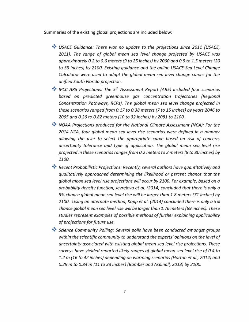
Summaries of the existing global projections are included below:

USACE Guidance: There was no update to the projections since 2011 (USACE,

2011). The range of global mean sea level change projected by USACE was

approximately 0.2 to 0.6 meters (9 to 25 inches) by 2060 and 0.5 to 1.5 meters (20

to 59 inches) by 2100. Existing guidance and the online USACE Sea Level Change

Calculator were used to adapt the global mean sea level change curves for the

unified South Florida projection.

IPCC AR5 Projections: The 5th Assessment Report (AR5) included four scenarios

based on predicted greenhouse gas concentration trajectories (Regional

Concentration Pathways, RCPs). The global mean sea level change projected in

these scenarios ranged from 0.17 to 0.38 meters (7 to 15 inches) by years 2046 to

2065 and 0.26 to 0.82 meters (10 to 32 inches) by 2081 to 2100.

NOAA Projections produced for the National Climate Assessment (NCA): For the

2014 NCA, four global mean sea level rise scenarios were defined in a manner

allowing the user to select the appropriate curve based on risk of concern,

uncertainty tolerance and type of application. The global mean sea level rise

projected in these scenarios ranges from 0.2 meters to 2 meters (8 to 80 inches) by

2100.

Recent Probabilistic Projections: Recently, several authors have quantitatively and

qualitatively approached determining the likelihood or percent chance that the

global mean sea level rise projections will occur by 2100. For example, based on a

probability density function, Jevrejeva et al. (2014) concluded that there is only a

5% chance global mean sea level rise will be larger than 1.8 meters (71 inches) by

2100. Using an alternate method, Kopp et al. (2014) concluded there is only a 5%

chance global mean sea level rise will be larger than 1.76 meters (69 inches). These

studies represent examples of possible methods of further explaining applicability

of projections for future use.

Science Community Polling: Several polls have been conducted amongst groups

within the scientific community to understand the experts’ opinions on the level of

uncertainty associated with existing global mean sea level rise projections. These

surveys have yielded reported likely ranges of global mean sea level rise of 0.4 to

1.2 m (16 to 42 inches) depending on warming scenarios (Horton et al., 2014) and

0.29 m to 0.84 m (11 to 33 inches) (Bamber and Aspinall, 2013) by 2100.

8

Projection confidence: The understanding of past sea level changes has improved since

the Work Group’s last review due to additional observations and analyses of processes

driving thermal expansion, loss of ice from ice sheets and glaciers and terrestrial water

storage by the scientific community. Despite this improved understanding, the

development of complex climate models is evolutionary and many processes and

responses are yet to be incorporated. The numerous ice melt accelerating feedbacks not

in the models are especially of concern as they are speeding up ice melt and sea level rise

well beyond model projections. Models do continue to offer useful approximations of

trends and order of magnitude of rates of change and acceleration based on climate data

input and are suitable for determining projected future ranges for planning and design

efforts. Additionally, as noted in Parris et al. (2012), the quadratic curves comprising the

projection were selected by the some of the scientific community for simplicity. Sea level

will not rise in the smooth manner illustrated by the quadratic curves but, may be

punctuated by faster and slower rates (Parris et al., 2013).

9

GUIDANCE FOR APPLICATION

INCREASE IN RECURRENT FLOODING AND REDUCED DRAINAGE CAPACITY

Recent analyses of tide gauge records acquired along the US Atlantic coast indicate a rapid

acceleration in the rate of sea level rise since 2000, which was attributed to possible slowing

down of the Atlantic Meridional Overturning Circulation (AMOC) (Ezer et al., 2013; Sallenger et

al., 2012; Yin et al., 2009). The higher sea level resulted in increasing flooding frequency in several

coastal communities, e.g., Boston, Norfolk, and Miami Beach (Ezer et al., 2013; Kirshen et al.,

2008; Kleinosky et al., 2007; Wdowinski et al., 2015). These frequent flood events, often termed

“nuisance flooding”, occur mainly due to heavy rain during high tide conditions but sometimes

occur due to high tide alone and are termed “King tides”, “lunar flooding” or “sunny sky flooding”.

Recently, Ezer and Atkinson (2014) used tide gauge data to calculate accumulated flooding time

in twelve locations along the Atlantic coast and showed a significant increase in flooding duration

over the past twenty years. They suggested that flood duration is a reliable indicator for the

accelerating rate of sea level rise, which is often difficult to estimate on a regional-scale.

On the national scale, NOAA (2014) published an assessment of nuisance flooding finding that

the duration and frequency of these events are intensifying around the United States.

Subsequently, Sweet and Park (2014) demonstrated that coastal areas are experiencing an

increased frequency of flood events (an acceleration) over the last few decades, and that this

acceleration in flood occurrence will continue regardless of the specific rate of sea level rise.

A detailed analysis of nuisance flooding occurrence in Miami Beach was conducted by Wdowinski

et al. (2015), who used a variety of data sources (tide gauge, rain gauge, media reports, insurance

claims, and photo records) from the past 16 years (1998-2013). They found that most flooding

events occur after heavy rain (> 80 mm, 3 inches) during high tide conditions, but also after the

fall equinox tides regardless of rain events. An analysis of flooding frequency over the past 16

years revealed that since 2006, rain-induced events increased by 33% and tide-induced events

quadrupled, from 2 events during 1998-2005 to 8-16 events in 2006-2013. Wdowinski et al.

(2015) also analyzed the nearby Virginia Key tide gauge record and found a significant

acceleration in the rate of sea level rise since 2006. The average rate of regional sea level rise

since 2006 is 9±4 mm/yr, significantly higher than the global average rate of 2.8±0.4 mm/yr

estimated from in-situ data (Church and White, 2011). Although the Work Group notes that

continued analysis of changes in trends over time is necessary to determine long-term

significance of this recently observed uptrend, studies have already begun to correlate the

regional sea level rise to the slowing down of the Gulfstream. A comparison between sea level

variations near Miami with high-resolution global climate model simulations (Kirtman et al.,

2012) revealed a strong correlation between increasing sea level rise in the Miami area and a

10

weakening of the Florida Current-Gulf Stream system. This finding confirmed concurs with other

studies that relate sea level rise acceleration along the US Atlantic coast with weakening of the

Gulf Stream (e.g., Ezer et al., 2013; Park and Sweet, 2015).

STORM SURGE AND SEA LEVEL RISE

Storm surge and sea level rise are independent coastal processes that when occurring

simultaneously lead to compounded impacts. Sea level rise will increase the inland areal extent

inundated by surges, the depth of flooding and power of the surge and the extent and intensity

of damage associated with storm surge and waves. As a result, severe storms of the future will

cause more damage than storms of equal intensity occurring at today’s sea level. Tebaldi et al.

(2012) estimate a 100-year magnitude surge flooding (by today’s standards) will begin to occur

every 20 years at the projected mean sea level in 2050. Regional hazard mapping does not yet

include the combined effects of sea level rise and surge but the impacts are anticipated to be

significant.

Historically, the sea level extremes have increased along with the increase in mean sea level at

locations along the coasts. Using this as the basis, one can relate the sea level extremes to mean

sea level which allows the determination of future extremes and return periods (Obeysekera and

Park, 2013). Another approach is to use the non-tidal residuals (component of storm surge and

waves above the tidal variations), NTR, and determine their probabilistic characteristics.

Assuming future sea level rise scenarios and the tidal variations, one can then superimpose

extreme storm surge of NTR for a given return period to determine total sea level extreme for a

given time epoch in the future. Return period for a given scenario can be determined using

methods outlined in Salas and Obeysekera (2014). Both approaches assume there is no change

in future “storminesss” although with higher sea levels, magnitude of storm surge may change

at some locations along the coasts.

NATURAL RESOURCE DEGRADATION

As sea level rise increasingly inundates coastal areas, there is the potential for degradation of

natural resources and loss of their services to the surrounding environment. Ecosystems will

transition either by retreat and migration, adaptation, or elimination of functions and certain

species. Shallow water habitats may transition to open water, forcing ecological changes in

coastal wetlands and estuaries affecting nesting, spawning and feeding locations and behavior.

Intrusion of saltwater inland, into inland water bodies and within the aquifer is negatively

impacting freshwater resources, and these impacts will worsen or accelerate with further sea

level rise. Inundation of shorelines will increase the extent and severity of beach erosion and

11

previously stable coastal areas. In combination, these impacts will cascade throughout the

region’s ecosystems even if they are not immediately adjacent to open water areas.

Natural infrastructure is critical to the resilience of the urban environment, in that it provides

many benefits related to storm protection, water and air purification, moderating urban heat

effects, and socio-economics. South Florida’s tourist economy is heavily dependent on these

natural resources. The region must prioritize providing space for habitat transitions and focus on

reducing anthropogenic pressures that would compound the degrading effects of sea level rise.

GUIDANCE IN APPLYING THE PROJECTIONS

AUDIENCES

The Unified Sea Level Rise Projection for Southeast Florida is intended to be used for planning

purposes by a variety of audiences and disciplines when considering sea level rise in reference to

both short and long-term planning horizons as well as infrastructure siting and design in the

Southeast Florida area. Potential audiences for the projections include, but are not limited to,

elected officials, urban planners, architects, engineers, developers, resource managers and public

works professionals.

One of the key values of the projection is the ability to associate specific sea level rise scenarios

with timelines. When used in conjunction with vulnerability assessments, these projections

inform the user of the potential magnitude and extent of sea level rise impact at a general

timeframe in the future. The blue shaded portion of the projection provides a likely range for sea

level rise values at specific planning horizons. Providing a range instead of a single value may

present a challenge to users such as engineers who are looking to provide a design with precise

specifications. Public works professionals and urban planners need to work with the engineers

and with policy makers to apply the projection to each project based on the nature, value,

interconnectedness, and life cycle of the infrastructure proposed.

Finally, elected officials should use the projections to inform decision making related to issues

such as adaptation policies, budget impacts associated with design features which address

planning for future sea level rise, capital improvement project needs especially those associated

with drainage and shoreline protection, and land use decisions.

APPLYING PROJECTION CURVES TO INFRASTRUCTURE SITING AND DESIGN

When determining how to apply the projection curves, the user needs to consider the nature,

value, interconnectedness, and life cycle of the existing or proposed infrastructure. The blue

12

shaded portion of the projection can be applied to most infrastructure projects, especially those

with a design life expectancy of less than 50 years. The designer of a type of infrastructure that

is easily replaced, has a short lifespan, is adaptable, and has limited interdependencies with other

infrastructure or services must weigh the potential benefit of designing for the upper blue line

with the additional costs. Should the designer opt for specifying the lower curve, she/he must

consider the consequences of under-designing for the potential likely sea level condition. Such

consequences may include premature infrastructure failure. Additionally, planning for

adaptation should be initiated in the conceptual phase. A determination must be made on

whether or not threats can be addressed mid-life cycle via incremental adaptation measures,

such as raising the height of a sluice gate on a drainage canal.

Forward thinking risk management is critical to avoiding loss of service, loss of asset value and

most importantly loss of life or irrecoverable resources. An understanding of the risks that critical

infrastructure will be exposed to throughout its life cycle such as sea level rise inundation, storm

surge and nuisance flooding must be established early on in the conceptual phase. If incremental

adaptation is not possible for the infrastructure proposed and inundation is likely, designing to

accommodate the projected sea level rise at conception or selection of an alternate site should

be considered. Projects in need of a greater factor of safety related to potential inundation

should consider designing for the upper limit of the blue-shaded zone. Examples of such projects

may include evacuation routes planned for reconstruction, communications and energy

infrastructure and critical government and financial facilities.

Due to the community’s fundamental reliance on major infrastructure, existing and proposed

critical infrastructure should be evaluated using the upper curve of the projection, the orange

curve (Figure 1, NOAA High). Critical projects include those or projects which are not easily

replaceable or removable, have a long design life (more than 50 years), or are interdependent

with other infrastructure or services. If failure of the critical infrastructure would have

catastrophic impacts, it is considered to be high risk. Due of the community’s critical reliance on

major infrastructure, existing and proposed high risk infrastructure should be evaluated using the

upper curve of the projection, the orange curve (Figure 1, NOAA High). Examples of high risk

critical infrastructure include nuclear power plants, wastewater treatment facilities, levees or

impoundments, bridges along major evacuation routes, airports, seaports, railroads, and major

highways.

For low risk infrastructure projects, the lowermost curve of the projection (Figure 1, IPCC AR5

RCP8.5 curve) may be applied. Low risk projects include infrastructure expected to be

constructed and then replaced within the next 10 years, projects that are easily replaceable and

13

adaptable or projects with limited interdependencies and limited impacts when failure occurs.

An example of such a project may be a small culvert in an isolated area.

Additionally, planning for adaptation should be initiated in the conceptual phase. A

determination must be made on whether or not risk can be addressed mid-life cycle via

incremental. If incremental adaptation is not possible for the type of high risk infrastructure

proposed and inundation is likely, designing to accommodate the projected sea level rise at

conception or selection of an alternate site should be considered. To ensure an appropriately

conservative design approach is used, the upper limit of the projection (Figure 1, NOAA High)

should be used for projects with design lives of more than 50 years.

AVAILABLE VULNERABILITY ASSESSMENTS

The Southeast Florida Regional Climate Change Compact and the individual Compact Counties

have developed region-wide and county-wide sea level rise inundation vulnerability assessments

available for public use (Compact, 2012). These assessments spatially delineate areas of

inundation correlating to 1 foot, 2 feet and 3 feet of sea level rise. In addition, the Compact

website hosts a multitude of sources of information, tools and links in support of adaptation and

mitigation planning for use by the Compact communities.

SUMMARY

The Work Group recommends the use of the NOAA High Curve, the USACE High Curve (USACE,

2015) and the median of the IPCC AR5 RCP8.5 scenario (IPCC, 2013) as the basis for a Southeast

Florida sea level rise projection for the 2030, 2060 and 2100 planning horizons. In the short term,

sea level rise is projected to be 6 to 10 inches by 2030 and 14 to 26 inches by 2060 (above the

1992 mean sea level). Sea level has risen 3 inches from 1992 to 2015. In the long term, sea level

rise is projected to be 31 to 61 inches by 2100. For critical infrastructure projects with design lives

in excess of 50 years, use of the upper curve is recommended with planning values of 34 inches

in 2060 and 81 inches in 2100. Sea level will continue to rise even if global mitigation efforts to

reduce greenhouse gas emissions are successful at stabilizing or reducing atmospheric CO2

concentrations; however, emissions mitigation is essential to moderate the severity of potential

impacts in the future. A substantial increase in sea level rise within this century is likely and may

occur in rapid pulses rather than gradually.

The recommended projection provides guidance for the Compact Counties and their partners to

initiate planning to address the potential impacts of sea level rise on the region. The shorter term

planning horizons (through 2060) are critical to implementation of the Southeast Florida Regional

14

Climate Change Action Plan, to optimize the remaining economic life of existing infrastructure

and to begin to consider adaptation strategies. As scientists develop a better understanding of

the factors and reinforcing feedback mechanisms impacting sea level rise, the Southeast Florida

community will need to adjust the projections accordingly and adapt to the changing conditions.

To ensure public safety and economic viability in the long run, strategic policy decisions will be

needed to develop guidelines to direct future public and private investments to areas less

vulnerable to future sea level rise impacts.

15

LITERATURE CITED

Bamber J. L., Aspinall, W. P. 2013. An expert judgement assessment of future sea level rise from the ice sheets. Nat Clim Change 3: 424−427

Bell, R. E., Tinto, K., Das, I., Wolovick, M., Chu, W., Creyts, T. T., ... & Paden, J. D. 2014. Deformation, warming and softening of Greenland [rsquor] s ice by refreezing meltwater. Nature Geoscience. Bintanja, R., Van Oldenborgh, G. J., Drijfhout, S. S., Wouters, B., & Katsman, C. A. 2013. Important role for ocean warming and increased ice-shelf melt in Antarctic sea-ice expansion. Nature Geoscience, 6(5), 376-379. Blewitt, G., Kreemer, C., Hammond, W.C., Gazeaux, J. 2015. MIDAS trend estimator for accurate GPS station velocities without step detection, Journal of Geophysical Research, in review. Bock, Y., Wdowinski, S., Ferretti, A., Novali, F., and Fumagalli, A. 2012. Recent subsidence of the Venice Lagoon from continuous GPS and interferometric synthetic aperture radar. Geochem. Geophys. Geosyst. 13. Q03023. doi:10.1029/2011GC003976. Calafat, F.M. and Chambers, D.P. 2013. Quantifying recent acceleration in sea level unrelated to internal climate variability. Geophys. Res. Lett. 40. 3661–3666. doi:10.1002/grl.50731. Church, J.A. and White, N.J. 2011. Sea-Level Rise from the Late 19th to the Early 21st Century. Surveys in Geophysics. 32(4-5). 585-602. doi:10.1007/s10712-011-9119-1. Collins, M., Knutti, R., Arblaster, J., Dufresne, J.-L., Fichefet, T., Friedlingstein, P., Gao, X., Gutowski, W.J., Johns, T., Krinner, G., Shongwe, M., Tebaldi, C., Weaver, A.J. & Wehner, M. 2013. Long-term Climate Change: Projections, Commitments and Irreversibility. In: Stocker T.F., Qin D., Plattner G.-K., Tignor M., Allen S.K., Boschung J., Nauels A., Xia Y., Bex V. & Midgley P.M. (eds.), Climate change 2013: the physical science basis. Contribution of Working Group I to the Fifth Assessment Report of the Intergovernmental Panel on Climate Change, Cambridge University Press, Cambridge, United Kingdom and New York, NY, USA. Ezer, T., Atkinson, L.P., Corlett, W.B., and Blanco, J.L. 2013. Gulf Stream’s induced sea level rise and variability along the U.S. mid-Atlantic coast. Journal of Geophysical Research: Oceans. 118. 685-697. Southeast Florida Regional Climate Change Compact (Compact). 2012. Analysis of the Vulnerability of Southeast Florida to Sea Level Rise. 181 p. http://www.southeastfloridaclimatecompact.org//wp-content/uploads/2014/09/vulnerability-assessment.pdf

16

Southeast Florida Regional Climate Change Compact Technical Ad hoc Work Group (Compact). 2011. A Unified Sea Level Rise Projection for Southeast Florida. A document prepared for the Southeast Florida Regional Climate Change Compact Steering Committee. 27 p. Ezer, T. and Atkinson, L.P. 2014. Accelerated flooding along the U.S. East Coast: On the impact of sea-level rise, tides, storms, the Gulf Stream, and the North Atlantic Oscillations. Earth's Future. 2. 362–382. doi:10.1002/2014EF000252. Flick, R., Knuuti, K., and Gill, S. 2012. Matching mean sea level rise projections to local elevation datums. Journal of Waterway, Port, Coastal, and Ocean Engineering. 139(2). 142–146. Gardner, A.S., Moholdt, G., Cogley, J.G., Wouters, B., Arendt, A.A., Wahr, J., Berthier, E., Hock, R., Pfeffer, W.T., Kaser, G., Ligtenberg, S.R.M., Bolch, T., Sharp, M.J., Hagen, J.O., van den Broeke, M.R., and Paul, F. 2013. A Reconciled Estimate of Glacier Contributions to Sea Level Rise: 2003 to 2009, Science. 340 (6134). 852-857. doi:10.1126/science.1234532. Greenbaum, J.S., Blankenship, D.D., Young, D.A., Richter, T.G., Roberts, J.L., Aitken, A.R.A., Legresy, B., Schroeder, D.M., Warner, R.C., van Ommen, T.D., and Siegert, M.J. 2015. Ocean access to a cavity beneath Totten Glacier in East Antarctica, Nature Geosci., publ. online 16 March doi:10.1038/NGEO2388, 2015. Hallberg, R., A. Adcroft, J. Dunne, J. Krasting, and R. J. Stouffer. 2013. Sensitivity of 21st century global-mean steric sea level rise to ocean model formulation. J. Clim. 26. 2947-2956. Hay, C. C., Morrow, E., Kopp, R. E., & Mitrovica, J. X. 2015. Probabilistic reanalysis of twentieth-century sea-level rise. Nature, 517(7535), 481-484. Hellmer, H. H., Kauker, F., Timmermann, R., Determann, J., & Rae, J. 2012. Twenty-first-century warming of a large Antarctic ice-shelf cavity by a redirected coastal current. Nature, 485(7397), 225-228. Horton, B.P., Rahmstorf, S., Engelhart, S.E., Kemp, A.C., 2014. Expert assessment of sea-level rise by AD 2100 and AD 2300. Quaternary Science Reviews. 84. 1-6. IPCC. 2013. Climate Change 2013. The Physical Science Basis. Contribution of Working Group I to the Fifth Assessment. Report of the Intergovernmental Panel on Climate Change [Solomon, S., Qin, D., Manning, M., Chen, Z., Marquis, M., Averyt, K.B., Tignor, M., and Miller, H.L. (eds.)]. Cambridge University Press: Cambridge, United Kingdom and New York. Jacob, T., Wahr, J., Pfeffer, W.T., Swenson, S. 2012. Recent contributions of glaciers and ice caps to sea level rise. Nature. 482. 514-518. Jacobs, S. S., Jenkins, A., Giulivi, C. F., & Dutrieux, P. 2011. Stronger ocean circulation and increased melting under Pine Island Glacier ice shelf. Nature Geoscience, 4(8), 519-523.

17

Jenkins, A., Dutrieux, P., Jacobs, S. S., McPhail, S. D., Perrett, J. R., Webb, A. T., & White, D. 2010. Observations beneath Pine Island Glacier in West Antarctica and implications for its retreat. Nature Geoscience, 3(7), 468-472. Jevrejeva, S., Grinstead, A., and Moore, J.C., 2014. Upper limit for sea level projections by 2100. Environ. Res. Lett. 9 (2014) 104008 (9pp). Johnson, G. C., McTaggart, K. E., & Wanninkhof, R. 2014. Antarctic Bottom Water temperature changes in the western South Atlantic from 1989 to 2014. Journal of Geophysical Research: Oceans, 119(12), 8567-8577. Joughin, I., & Alley, R. B. 2011. Stability of the West Antarctic ice sheet in a warming world. Nature Geoscience, 4(8), 506-513. King, M. A., Bingham, R. J., Moore, P., Whitehouse, P. L., Bentley, M. J., & Milne, G. A. 2012. Lower satellite-gravimetry estimates of Antarctic sea-level contribution. Nature, 491(7425), 586-589. Kirshen, P., Knee, K., and Ruth, M. 2008. Climate change and coastal flooding in Metro Boston: impacts and adaptation strategies. Climatic Change. 90(4). 453-473. doi:10.1007/s10584-008-9398-9. Kirtman, B.P., Bitz, C., Bryan, F., Collins, W., Dennis, J., Hearn, N., KinterIII, J.L., Loft, R., Rousset, C., Siqueira, L., Stan, C., Tomas, R., Vertenstein, M. 2012. Impact of ocean model resolution on CCSM climate simulations. Climate Dynamics. 39(6). 1303-1328. doi:10.1007/s00382-012-1500-3. Kleinosky, L.R., Yarnal, B., and Fisher, A. 2007. Vulnerability of Hampton Roads, Virginia to storm-surge flooding and sea-level rise. Natural Hazards. 40(1). 43-70. doi:10.1007/s11069-006-0004-z. Kopp, R.E., Horton, R.M., Little, C.M., Mitrovica, J.X., Oppenheimer, M., Rasmussen, D.J., Strauss, B.H., and Tebaldi, C. 2014. Probabilistic 21st and 22nd century sea-level projections at a global network of tide-gauge sites. Earth's Future. 2(8). 383-406. doi:10.1002/2014EF000239. Morlighem, M., Rignot, E., Mouginot, J., Seroussi, H., & Larour, E. 2014. Deeply incised submarine glacial valleys beneath the Greenland ice sheet. Nature Geoscience, 7(6), 418-422. NASA/Jet Propulsion Laboratory. "Warming seas and melting ice sheets." ScienceDaily. ScienceDaily, 26 August 2015. www.sciencedaily.com/releases/2015/08/150826111112.htm . Nevada Geodetic Laboratory. 2015. “CHIN Station Data” http://geodesy.unr.edu/NGLStationPages/stations/CHIN.sta

18

NOAA, 2015. “Mean Sea Level Trend, 8724580 Key West, Florida.” http://tidesandcurrents.noaa.gov/sltrends/sltrends_station.shtml?stnid=8724580 NOAA, 2014. Sea Level Rise and Nuisance Flood Frequency Changes around the United States. Technical Report NOS CO-OPS 073. Sweet W. V., Park J., Marra J., Zervas C., Gill S. http://tidesandcurrents.noaa.gov/publications/NOAA_Technical_Report_NOS_COOPS_073.pdf Obeysekera, J. and Park, J. 2013. Scenario-based projection of extreme sea levels. Journal of Coastal Research. Vol. 29, Issue 1, 1-7. Overduin, P., Grigoriev, M.N., Schirrmeister, L., Wetterich, S., Nätscher, V., Günther, F., Liebner, S., Knoblauch, C. and Hubberten, H. W. 2014. Permafrost degradation and methane release in the central Laptev Sea. 4th European Conference on Permafrost, Evora. 18 June 2014 - 21 June 2014. Park, J. and Sweet, W. 2015. Accelerated sea level rise and Florida Current transport. Ocean Sci., 11, 607-615, doi:10.5194/os-11-607-2015. Parris, A., Bromirski, P., Burkett, V., Cayan, D., Culver, M., Hall, J., Horton, R., Knuuti, K., Moss, R., Obeysekera, J., Sallenger, A., and Weiss, J. 2012. Global Sea Level Rise Scenarios for the US National Climate Assessment. NOAA Tech Memo OAR CPO-1. Pritchard, H. D., Ligtenberg, S. R. M., Fricker, H. A., Vaughan, D. G., Van den Broeke, M. R., & Padman, L. 2012. Antarctic ice-sheet loss driven by basal melting of ice shelves. Nature, 484(7395), 502-505. Rahmstorf, S., Feulner, G., Mann, M. E., Robinson, A., Rutherford, S., & Schaffernicht, E. J. 2015. Exceptional twentieth-century slowdown in Atlantic Ocean overturning circulation. Nature Climate Change. Rampal, P., Weiss, J., Dubois, C., & Campin, J. M. 2011. IPCC climate models do not capture Arctic sea ice drift acceleration: Consequences in terms of projected sea ice thinning and decline. Journal of Geophysical Research: Oceans (1978–2012), 116(C8). Rignot, E., Velicogna, I., van den Broeke, M.R., Monaghan, A., and Lenaerts, J. 2011. Acceleration of the contribution of the Greenland and Antarctic ice sheets to sea level rise. Geophysical Research Letters. 38. L05503. doi:10.1029/2011GL046583. Rye, C. D., Garabato, A. C. N., Holland, P. R., Meredith, M. P., Nurser, A. G., Hughes, C. W., ... & Webb, D. J. 2014. Rapid sea-level rise along the Antarctic margins in response to increased glacial discharge. Nature Geoscience, 7(10), 732-735.

19

Salas, J. and Obeysekera, J. 2014. Revisiting the concepts of return period and risk for nonstationary hydrologic extreme events. J. Hydrol. Eng., 19(3), 554–568. Sallenger, A.H., Doran, K.S., and Howd, P.A. 2012. Hotspot of accelerated sea-level rise on the Atlantic coast of North America. Nature Clim. Change. 2(12). 884-888. doi:10.1038/nclimate1597. Santamaría-Gómez, A., Gravelle, M., Collilieux, X., Guichard, M., Míguez, B.M., Tiphaneau, P., Wöppelmann, G. 2012. Mitigating the effects of vertical land motion in tide gauge records using a state-of-the-art GPS velocity field, Global and Planetary Change. 98-99. 6-17. http://dx.doi.org/10.1016/j.gloplacha.2012.07.007. Schuur, E.A.G., Abbott, B.W., Bowden, W.B., Brovkin, V., Camill, P., Canadell, J.G., Chanton, J.P., Chapin, F.S., III, Christensen, T.R., Ciais, P., Crosby, B.T., Czimczik, C.I., Grosse, G., Harden, J., Hayes, D.J., Hugelius, G., Jastrow, J.D., Jones, J.B., Kleinen, T., Koven, C.D., Krinner, G., Kuhry, P., Lawrence, D.M., McGuire, A.D., Natali, S.M., O’Donnell, J.A., Ping, C.L., Riley, W.J., Rinke, A., Romanovsky, V.E., Sannel, A.B.K., Schädel, C., Schaefer, K., Sky, J., Subin, Z.M., Tarnocai, C., Turetsky, M.R., Waldrop, M.P., Walter Anthony, K.M., Wickland, K.P., Wilson, C.J., Zimov, S.A., 2013. Expert assessment of vulnerability of permafrost carbon to climate change. Climatic Change. 119. 2. 359-374. Smeed, D.A., McCarthy, G.D., Cunningham, S.A., Frajka-Williams, E., Rayner, D., Johns, W.E., Meinen, C.S., Baringer, M.O., Moat, B.I., Duchez, A., and Bryden, H.L. 2014. Observed decline of the Atlantic meridional overturning circulation 2004–2012. Ocean Sci. 10. 29-38. doi:10.5194/os-10-29-2014. Snay, R., Cline, M., Dillinger, W., Foote, R., Hilla, S., Kass, W., Ray, J., Rohde, J., Sella, G., and Soler, T. 2007. Using global positioning system-derived crustal velocities to estimate rates of absolute sea level change from North America tide gauge records. J. Geophys. Res. 112. B04409. doi:10.1029/2006JB004606. Spence, P., Griffies, S.M., England, M.H., Hogg, A.M., Saenko, O.A., Jourdain, N.C. 2014. Rapid subsurface warming and circulation changes of Antarctic coastal waters by poleward shifting winds. Geophysical Research Letters. 41. 4601–4610. doi:10.1002/2014GL060613. Sweet, W.V. and Park, J. 2014. From the extreme to the mean: Acceleration and tipping points of coastal inundation from sea level rise. Earth's Future, 2: 579–600. doi:10.1002/2014EF000272. Talpe, M., Nerem, R.S., and Lemoine, F. 2014. G21C-02 Two decades of ice melt reconstruction in Greenland and Antarctica from time-variable gravity. Amer. Geophysical Union, Abstract G21C-02, Ann. Natl. Mtg. Tebaldi, C., Strauss, B.H., Zervas, C. E. 2012. Modelling sea level rise impacts on storm surges along US coasts. Environ. Res. Lett. 7 (2012) 11 pp.

20

USACE. 2015. USACE Sea Level Change Curve Calculator (2015.46) http://www.corpsclimate.us/ccaceslcurves.cfm USACE. 2013. Incorporating sea level change in civil works programs. Department of the Army Regulation No. 1100-2-8162, 31 December 2013. U.S. Army Corps of Engineers, CECW-CE, Washington D.C. USACE. 2011. Sea-Level Change Considerations in Civil Works Programs. Department of the Army Engineering Circular No. 1165-2-212, 1 October 2011. U.S. Army Corps of Engineers, CECW-CE, Washington, D.C. Velicogna, I., T. C. Sutterley, and M. R. van den Broeke. 2014. Regional acceleration in ice mass loss from Greenland and Antarctica using GRACE time-variable gravity data. J. Geophys. Res. Space Physics. 41. 8130–8137. doi:10.1002/2014GL061052. Vinther, B. M., Buchardt, S. L., Clausen, H. B., Dahl-Jensen, D., Johnsen, S. J., Fisher, D. A., ... & Svensson, A. M. 2009. Holocene thinning of the Greenland ice sheet. Nature, 461(7262), 385-388.

Watson, C.S., White, N.J., Church, J.A., King, M.A., Burgette, R.J. & Legresy, B. 2015. Unabated global mean sea-level rise over the satellite altimeter era. Natrure Climate Change, 5, 565-568. http://www.nature.com/nclimate/journal/v5/n6/full/nclimate2635.html

Wdowinski, S., Bray, R., Kirtman, B., and Wu, Z. 2015. Increasing flooding frequency and accelerating rates of sea level rise in Miami Beach, Florida. Submitted, Envir. Res. Let. Yin, J., Schlesinger, M.E., and Stouffer, R.J. 2009. Model projections of rapid sea-level rise on the northeast coast of the United States. Nature Geosci. 2(4). 262-266. doi:10.1038/ngeo462. http://www.nature.com/ngeo/journal/v2/n4/suppinfo/ngeo462_S1.html.

21

APPENDIX A: STAND ALONE GUIDANCE DOCUMENT AND PROJECTION

The Southeast Florida Regional Climate Change Compact’s 2015 Unified Sea Level Rise Projection

is presented below showing the anticipated range of sea level rise for the region from 1992 to

2100 (Figure 1). The projection highlights three planning horizons:

1) Short term, by 2030, sea level rise is projected to be 6 to 10 inches above 1992 mean

sea level;

2) Medium term, by 2060, sea level rise is projected to be 14 to 26 inches above 1992

mean sea level with the less likely possibility of extending to 34 inches;

3) Long term, by 2100, sea level rise is projected to be 31 to 61 inches above 1992 mean

sea level with the less likely possibility of extending to 81 inches.

The Unified Sea Level Rise Projection for Southeast Florida include three curves, named after the

global sea level rise curves from which they were derived: the NOAA High Curve (orange solid),

the USACE High Curve (blue solid) and the median of the IPCC AR5 scenario (blue dashed). The

blue shaded area represents the likely range of sea level rise for our region. The orange curve

represents a condition that is possible but less likely. The USACE Intermediate or NOAA

Intermediate Low curve is displayed on the figure for reference (green dashed curve). This

scenario would require significant reductions in greenhouse gas emissions in order to be plausible

and does not reflect the impact on sea level from the current emissions trends.

When determining how to apply the projection curves, the user needs to consider the nature,

value, interconnectedness, and life cycle of the infrastructure in question. The following guidance

is provided for using the projection.

22

The shaded zone between the IPCC AR5 median curve and the USACE High is

recommended to be generally applied to most projects within a short to long-term

planning horizon, especially those with a design life expectancy of less than 50 years.

The designer of a type of infrastructure that is easily replaced, has a short lifespan, is

adaptable, and has limited interdependencies with other infrastructure or services

must weigh the potential benefit of designing for the upper blue line with the

additional costs. Should the designer opt for specifying the lower curve, he must

consider the consequences of under designing for the potential likely condition.

The uppermost boundary of the projection (orange curve) should be utilized for

planning of critical infrastructure to be constructed after 2060 or projects with a long

design life (more than 50 years) as a conservative estimate of potential sea level rise.

Critical projects include those which are not easily replaceable or removable, have a

long design life (more than 50 years), or are interdependent with other infrastructure

or services. If failure of the infrastructure would have catastrophic impacts on the

economy, community or environment, it should be considered critical.

To reference the projection to the current year i.e. 2015, simply subtract the values listed in the

table below from the projected sea level rise. For example, based on the projection, sea level rise

in 2030 will be 6 to 10 inches above 1992 mean sea level. In order to determine how much rise

will occur relative to the current year, 2015, the values listed in the table below for the IPCC AR5

median and USACE High curves can be subtracted from the projected range i.e. 6-3=3 inches for

the lower end of the range and 10-4.3=5.6 inches for the upper end of the range, respectively.

The projection can be restated as such: sea level will rise 3 to 5.6 inches from this year (2015) to

2030.

Current Year IPCC AR5 Median

(Blue Dashed Line)

USACE High

(Blue Solid Line)

NOAA High

(Orange Line)

2015 3 4.3 5.3

2016 3.1 4.7 5.6

2017 3.4 4.9 6

2018 3.5 5.3 6.4

2019 3.7 5.5 6.8

To convert local relative sea level rise datum from mean sea level to a topographic reference

point used in surveying land elevations (NAVD 88), add the number listed in the table below to

projected sea level rise:

23

To convert relative sea level rise datum from mean sea level to feet

NAVD 88*, add the number below to value from

projection

To convert relative sea level rise datum from

mean sea level to inches NAVD 88, add the number

below to value from projection

Mean High Water (MHW)

Mean Low Water (MLW)

Mean Sea Level in feet NAVD 88

Mean Sea Level in inches NAVD 88

Inches NAVD 88

Inches NAVD 88

Key West -0.87 -10.4 -5.6 -14.2

Vaca Key -0.83 -10 -5.6 -14.2

Miami Beach

-0.96 -11.5 3.0 -26.5

Lake Worth Pier

-0.95 -11.4 4.9 -27.8

*North American Vertical Datum of 1988 (NAVD 88) is the topographic reference point used in surveying land elevations. By definition it is the vertical control datum of orthometric height established for vertical control surveying in the United States of America based upon the General Adjustment of the North American Datum of 1988.

Alternatively, the USACE Sea Level Change Curve Calculator (Version 2018.88) (USACE, 2015)

found at this website http://www.corpsclimate.us/ccaceslcurves.cfm can be used to change

datums, reference years and tide gauge locations. The projection curves were generated using

this tool.

The equations used for the curves comprising the unified sea level rise projection are as follows:

NOAA High Curve (Parris, 2012) and USACE High Curve (USACE, 2013):

E(t2) – E(t1)= a(t2 – t1) + b(t22 – t1

2)

where E(t2) – E(t1) = Eustatic sea level change (m) with reference

year of 1992;

t1 = difference in time between current year or construction date

and 1992 e.g. 2015-1992 = 23 years;

t2 = difference in time between future date of interest and 1992 i.e.

2060-1992 = 68 years;

where a is a constant equal to 0.0017 m/yr, representing the rate

of global mean sea level change,

24

and b is a variable equal to 1.56x10-4 for the NOAA High Curve;

1.13x10-4 for the USACE high curve, representing the acceleration

of sea level change.

IPCC AR5 RCP8.5 Median Curve (IPCC, 2013):

E(t2) – E(t1)= 0.0017(t2 – t1) + (4.684499x10-5)(t22 – t1

2)

The NOAA Intermediate Low/ USACE Low curve that is not part of the projection

but included on the graph for reference (green dashed line) can be derived as

follows:

E(t2) – E(t1)= 0.0017(t2 – t1) + (2.71262x10-5)(t22 – t1

2)

The equations above are global mean sea level rise projections. In order to adapt the curves for

regional use, the average rate of mean sea level rise or “a” value is adjusted. For example, to

reference the above equations to the Key West tide gauge, a equals 0.0022 m/yr.

25

Figure A-1: Unified Sea Level Rise Projection. These projections are referenced to mean sea level at the Key West tide gauge. The projection

includes three global curves adapted for regional application: the median of the IPCC AR5 scenario as the lowest boundary (blue dashed curve),

the USACE High curve as the upper boundary for the short term for use until 2060 (solid blue line), and the NOAA High curve as the uppermost

boundary for medium and long term use (orange solid curve). The incorporated table lists the projection values at years 2030, 2060 and 2100.

The USACE Intermediate or NOAA Intermediate Low curve is displayed on the figure for reference (green dashed curve). This scenario would

require significant reductions in greenhouse gas emissions in order to be plausible and does not reflect current emissions trends.

26

APPENDIX B: STATE OF SCIENCE UPDATE

ACCELERATION OF SEA LEVEL RISE

A statistically significant acceleration of sea level rise has been documented in the latter half of

the 20th century continuing through recent years (Church and White, 2011; Calafat and

Chambers, 2013; Hay et al. 2015; IPCC, 2013; Watson et al., 2015). Hay et al. (2015) reported the

global sea level rise rate from 1901 to 1990 to be 1.2 +/- 0.2 mm/yr (a value which had been

overestimated in previous studies). Since 1993, an increase in the average global mean sea level

rise rate has been observed (Hay et al., 2015; Watson et al., 2015). Watson et al. (2015) has most

recently reported the average global mean sea level rise rate to be more than double the rate of

the previous century, indicating an acceleration; the observed rate was 2.6+0.4 mm/yr from 1993

to 2015 with an acceleration of 0.04 mm/yr2. This acceleration indicates sea level will rise more

rapidly in the future than it has historically. The global and regional processes driving sea level

rise and its acceleration are discussed in the following sections.

FACTORS INFLUENCING SEA LEVEL RISE

GLOBAL PROCESSES

In 2011, the Work Group noted studies describing a variety of reinforcing (positive) feedbacks

that are accelerating ice sheet melt in Greenland and Antarctica and also accelerating Arctic pack

ice melt, permafrost thaw and organic decay, and methane hydrate release from the warming

Siberian Shelf, in addition to other global processes affecting sea level rise i.e. increasing

greenhouse gas concentrations, changes in volcanic forcing and tropospheric aerosol loading

(Compact, 2011). Since then, numerous additional reinforcing feedbacks have been documented

and previously recognized feedbacks have intensified.

ACCELERATION OF ICE MELT

Accelerated melting of the ice sheets on Greenland and Antarctica (Rignot et al., 2011; Talpe et

al., 2014) is expected to be the predominant factor affecting sea level rise acceleration during

the 21st Century. Melting is caused by increasing temperatures and warming of the atmosphere,

warm currents moving along the coast of Greenland, and warm ocean water moving under and

up into ice sheets through deep outlet glacial fjords in Antarctica. Recent observations have

indicated ice sheets are more vulnerable to melting than previously realized due to the extent of

deep valleys within the ice sheets connecting warmer ocean water to the internal areas of the

ice sheets thus causing rapid melting and peripheral thinning (Jenkins et al., 2010; Jacobs et al.,

2011; Morlighem et al., 2014; Rignot et al., 2014; Greenbaum et al., 2015). Accelerated melting

results in large discharges of fresh water which raises the local sea level near the ice sheets (8

27

inches around Antarctica over past 20 years) (Rye et al., 2014). This release of freshwater has

resulted in a seasonal increase in the amount of sea ice in the Antarctic (Bintanja et al., 2013; Rye

et al., 2014) and slower circulation of North Atlantic surface water, also known as Atlantic

Meridional Overturning Circulation (Rahmstorf et al., 2015). The slowdown in circulation may

contribute to increased local sea level rise along the Florida coast, as discussed in the Regional/

Local Processes section. The IPCC projections do not include the factors related to acceleration

of ice melting processes described above, and as a result are likely an underestimate of future

sea level rise (Rignot et al., 2011).

ICE SHEET DISINTEGRATION

Indicators of ice sheet disintegration include retreat of the ice sheet’s outer boundary and rapid

thinning. Lateral flow of the Greenland Ice Sheet margin, the outer boundary, has dramatically

accelerated in the past two decades in response to surface melt waters penetrating fractures in

the ice and warming and softening the ice (Bell et al., 2014). In addition to retreat, the ice sheets

have initiated a rapid thinning process due to basal melt (Pritchard et al., 2012), signaling the

initiation of prolonged ice sheet degradation based on historic analysis (Johnson et al., 2014).

Joughin et al. (2011) have used numerical models to look at the sensitivity of the outlet glaciers

of the West Antarctic Ice Sheet to ocean water melt and have concluded that the West Antarctic

Ice Sheet collapse is already underway; the extent of the collapse in the future is not yet known.

As part of the Gravity Recovery and Climate Experiment (GRACE) satellite monitoring program,

ice sheet mass loss has been quantified as 280±58 gigatons per year (Gt/yr) from Greenland and

up to 180±10 Gt/yr in Antarctica (Velicogna et al., 2014). As a reference for the magnitude of a

gigaton, one could estimate one gigaton to equal the mass of over one hundred million

elephants. In addition, significant recent work was completed to verify the estimated

contribution of ice sheet disintegration to sea level rise using satellite data (Jacob et al., 2012;

King et al., 2012; Gardner et al., 2013) with the conclusion that ice sheet melt accounted for

29±13% of sea level rise from 2003 to 2009 (Gardner, 2013). In order to further refine the

estimates and projections of the magnitude of ice sheet degradation and their contribution to

sea level rise, the complex dynamics driving ice sheet melt need to be better understood, in

particular the mechanisms driving interactions between ice sheets and warm currents.

WARM CURRENTS

In 2011, the Work Group acknowledged the effects of warm ocean water currents accelerating

summer pack ice melt and causing melting beneath the outlet glaciers. Recent work has further

clarified the compounding mechanisms driving the flow and temperature changes of warm

currents. Spence et al. (2014) analyzed the poleward shift in direction of the southern

hemisphere westerly winds since the 1950’s and simulated the intense warming of coastal waters

28

associated with such a shift in order to explain and forecast the significant temperature increase

in ocean waters interacting with the base of ice sheets and floating ice shelves. This study serves

to validate the projection of the persistence of this wind trend and the resulting melting due to

warm current interaction. Separate from wind forcing, an increase in ocean surface stress due to

thinning of the formerly consolidated sea-ice cover near Antarctica is proposed to result in a

redirection of warm ocean currents into submarine glacial troughs and further expediting melting

of the deep ice-shelf base based on ocean-ice modeling (Hellmer et al., 2012). Ice sheet melt as

a result of interaction with warm currents is one of the dominant factors contributing to recent

global sea level rise (IPCC, 2013); however, as discussed in the next section, land based

contributions to global warming may further exacerbate sea level rise in the future.

THAWING PERMAFROST

The potential for significant additional emissions of carbon dioxide and methane from thawing

permafrost and the rate of occurrence continues to be investigated. The intricate feedback

mechanisms associated with permafrost are not well understood; as such, the IPCC did not

include permafrost thaw in its projections (Collins et al., 2013). This deficiency was criticized

publicly due to the theorized potential for permafrost carbon emissions to exceed emissions from

fossil fuel use. Schuur et al. 2013 conducted a survey of experts to quantify permafrost change

in response to four global warming scenarios and found despite risk for significant contributions

of emissions from thawing, fossil fuel combustion was likely to remain the main source of

emissions and climate forcing until 2100 based on the proposed warming scenarios.

Following the release of the IPCC (2013) report, demand for research to understand the dynamics

of the physical and chemical permafrost processes has increased in order to confirm the

estimates of emissions from thawing. As an initial step, the occurrence of significant submarine

permafrost thawing was confirmed by Overduin et al. (2014) when 8 to 10°C of warming within

the permafrost layer was observed in less than 1,000 years, resulting in a degradation of ice-

bearing permafrost at the rate of 3 cm/yr. In addition, seawater seeping through soil pores was

identified as the source of sulfate necessary to oxidize methane in the upper layer of the thawing

permafrost. Although site specific, studies such as Overduin et al. (2014) will begin to provide the

information necessary to incorporate permafrost thawing into models and projections in the near

future.

REGIONAL/ LOCAL PROCESSES

VERTICAL LAND MOVEMENT

Vertical earth movements, which regionally and locally modify the globally averaged rate of sea

level change, result in a relative rate of change that varies from one location to another. These

29

land motions have been inferred from historical tide data and geodesic measurements. When

added to projected rates of global mean sea level rise, they result in a perceived change ranging

from increased rise in regions of subsidence (e.g., New Orleans) to falling sea levels where the

land is being uplifted (e.g., along the northern border of the Gulf of Alaska). Other regions are

geologically stable and have only small differences with respect to the global rate of change. In

South Florida, in general, coastal land elevations are considered to be relatively stable meaning

that the land is not experiencing significant uplift nor subsidence. It is also important to note, the

vertical land movement that is occurring is non-uniform across South Florida and movement

measured at specific monitoring stations sites may not reflect vertical land movement in adjacent

areas.

The Continuously Operating Reference (COR) network of permanent Global Positioning System

(GPS) receivers provides precise measurements of vertical land movement in four locations

throughout Southeast Florida (Key West, Virginia Key, Pompano Beach, and Palm Beach) over

periods of nine to eleven years. Additional continuous GPS measurements have been acquired in

eight other sites in the region over various time periods (two to eleven years). Precise analysis of

these data reveals negligible vertical movements at most stations (less than 1 mm/yr) (Snay et

al., 2007; Santamaría-Gómez et al., 2012; NGL, 2015). However, some stations show 1 to 6 mm/yr

of subsidence, reflecting mostly local unstable conditions of the GPS antenna monument (e.g.,

local building movements) (e.g., Bock et al., 2012).

National Geodetic Survey has operated continuous GPS stations at Key West, Fort Lauderdale,

Miami and Palm Beach Gardens. The GPS data of these sites were processed by the Nevada

Geodetic Laboratory, who presents the results at GPS time series

(http://geodesy.unr.edu/index.php). The rates of vertical land movement at these stations are

shown in Table 1 (Blewitt et al., 2015). It should be noted vertical land movement is non-uniform

across South Florida as a result of geology variations and the non-uniform compaction of fill

placed during development of the region. Subsidence at tide stations is closely monitored to

ensure the accuracy of sea level rise measurements. The regional rate of sea level rise is affected

by such localized subsidence and is accounted for in the regional sea level rise acceleration

variable incorporated in the projections adapted for the region.

30

Table 1: Continuous GPS Operation in Southeast Florida (Blewitt et al., 2015)

Site Location Duration Vertical rate

(mm/yr)

KYW1 Boca Chica Key 1997-2008 -0.5 ± 0.1

KYW5 Boca Chica Key 2007-present 0.1 ± 0.1

KYW6 Boca Chica Key 2007-present 1.0 ± 0.1 (uplift)

KWST Key West airport 2003-present -1.5 ± 0.1

CHIN Key West, 500 m south of

tide gauge 2008-presnt -1.6 ± 0.5

LAUD Fort Lauderdale Executive

Airport

2005-2014;

2014-2015 -0.5± 1.1

ZMA1 Miami Airport 2004-2008;

2008-present 0.2± 0.9

FLC6 Florida City 2009-present -1.8± 1.2

PBCH North Palm Beach County

Airport 2005-present 1.0± 1.0 (uplift)

Additionally, in some regions, the effects of changing ocean currents can further modify the

relative local rate of sea level rise. Such is the case of the east coast of Florida, as is discussed in

the next section, Ocean Dynamics, Gulfstream/ Circulation

OCEAN DYNAMICS, GULFSTREAM/ CIRCULATION

Ocean circulation has changed little during the current period of scientific observation, but in the

future it can considerably alter the relative rate of sea level rise in some regions, including

Southeast Florida. A slowing of the Florida Current and Gulf Stream will result in a more rapid sea

level rise along the east coast of North America. By 2100, these circulation changes could

contribute an extra 8 inches of sea level rise in New York and 3 inches in Miami according to Yin

et al. (2009). Most of the global climate models used by the IPCC (IPCC, 2007; 2013) project a 20-

30% weakening of the Atlantic Meridional Overturning Circulation (AMOC), of which the Gulf

Stream and Florida Current are a part. Measurements of the AMOC have yet to conclusively

detect the beginning of this change, however there has been a report of a recent decline in AMOC

strength by Smeed et al. (2014) that coincides with the mid-Atlantic hotspot of sea level rise

reported by Ezer et al. (2013) and Rahmstorf et al. (2015). Recent analysis of the Florida Current

transport has detected a decrease in circulation over the last decade, which appears to account

31

for 60% of South Florida sea level rise over the decade and contribute to a positive acceleration

(Park and Sweet, 2015). If a long-term slowdown of the AMOC and Florida Current. Rahmstorf

et al. (2015) use a proxy method also suggesting that a slowdown of the AMOC has begun. If a

long-term slowdown of the AMOC does occur, sea level rise along the Florida east coast could

conceivably be as much as 20 cm (8 inches) greater than the global value by 2100.

According to the most recent estimates by the IPCC (IPCC 2013, FigureB-1), the combined

differential due to regional ocean heating and circulation change along the Southeast Florida

coast would be in the range of 10%-20% greater than the globally averaged rise by 2090. For a

median (50% probability) sea level rise of one meter by 2100, this would give about 10-20 cm (4-

8 inches) of additional rise along the Southeast Florida coast, which is within the range of

estimates by Yin et al. (2009). However, the IPCC models do not have the horizontal resolution

required to effectively estimate these changes at the scale of the Florida Current and more

research with higher resolution ocean models will be required. As such, it is prudent to add ~15%

to the global mean sea level rise values projected by the IPCC in order to use them for Southeast

Florida planning. This adjustment is accounted for in the regional sea level rise coefficients

incorporated in the projections adapted for the region.

32

Figure B-1. Percentage of the deviation of the ensemble mean regional relative sea level

change between 1986-2005 and 2081-2100 from the global mean value, based on Figure

13.21, IPCC (2013). The figure was computed for RCP4.5, but to first order is representative

for all Representative Concentration Pathways (RCP). RCPs are the four greenhouse gas

concentration trajectories adopted by the IPCC for its fifth Assessment Report (AR5).

33

APPENDIX C: WORKGROUP COMMENTARY AND RECOMMENDATIONS

The following are recommendations made by the Work Group for consideration by the Southeast

Florida Regional Climate Compact Steering Committee to be used by the Compact Counties as

part of the implementation of the Regional Climate Change Action Plan.

a. The unified SE FL sea level rise projection will need to be reviewed as the scientific

understanding of ice melt dynamics improves. The projection should be revised within

five years of final approval of this document by the Southeast Regional Climate Change

Compact Steering Committee. This timing is consistent with the release of

Intergovernmental Panel on Climate Change Sixth Assessment Report which will provide

a synthesis of the major findings in climate science to date.

b. Users of the projection should be aware that at any point of time, sea level rise is

a continuing trend and not an endpoint.

c. The planet is currently on a high emissions trajectory for which committed sea level rise

is probably near the high end of the ranges. It should also be noted that the attenuation

of impacts through mitigation will not likely be sufficient to overcome the inertia of the

climate system prior to 2060.

d. Full and complete transparency of the projection and its implications should be promoted

across the communities in order to encourage and guide effective and realistic planning,

obtain realistic economic realities for maintaining functional infrastructure, insuring

social and economically sound further development, and necessary adaptation.

e. Further work to develop projections for the occurrence of extreme events in tandem with

sea level rise may be necessary to assist communities in planning for storm drainage

adaptation.

34

APPENDIX D: ACKNOWLEDGEMENT OF PARTICIPANTS

The Southeast Florida Regional Climate Change Compact Counties (Monroe, Miami-Dade,

Broward and Palm Beach Counties) and their partners wish to acknowledge the Work Group

participants and members of the SE FL Regional Climate Change Compact Steering Committee

for participating in meetings to support the development of the Unified Sea Level Rise Projection

and the guidance document. The following members contributed to the development and

refinement of the projection:

Danchuk, Samantha, Ph.D., P.E.

Berry, Leonard, Ph.D.

Enfield, David, Ph.D.

Gassman, Nancy, Ph.D.

Harlem, Peter, Ph.D.

Hefty, Nichole

Heimlich, Barry

Jurado, Jennifer, Ph.D.

Kivett, Jeff, P.E.

Landers, Glenn, P.E.

Murley, Jim

Obeysekera, Jayantha, Ph.D., P.E.

Park, Joseph, Ph.D., P.E.

Steelman, Marcia, C.F.M

Van Leer, John, Ph.D.

Wanless, Hal, Ph.D.

Wdowinski, Shimon, Ph.D.

35

APPENDIX E: DEVIATION FROM 2011 PROJECTION

The updated unified sea level rise projection includes the range projected by the 2011 unified

sea level rise projection with three enhancements. As described in previous paragraphs, the year

the projection begins was shifted from 2010 to 1992. Since the projection now references the

sea level rise that has occurred since 1992 instead of 2010, the values in the projection are larger

as a result of the sea having 8 more years to rise. For example, at the lower boundary of the

projection, by 2030, sea level rise is projected to be 5 inches above the where mean sea level was

in 1992. This is the exact same projected elevation as 3 inches above where the mean sea level

was in 2010, just a different elevation datum. Table 1 shows the adjustment of values from the

2011 Unified Projection with a reference (starting) year of 1992. Please note the lower boundary

is the same in both the 2011 and 2015 projections. The second enhancement to the projection

was the extension of the projection past 2060 continuing to 2100. The third enhancement to the

projection was the addition of the NOAA High Curve as the upper boundary after Year 2060. For

critical infrastructure projects with design lives in excess of 50 years, use of the upper curve is

recommended with planning values of up to 34 inches in 2060 and up to 81 inches in 2100.

Table 2: Comparison of Unified Projection in 2011 and 2015 at Key West

Year

2011 Unified Projection

(referenced to Year 2010) (inches above msl)

2011 Unified Projection

(adjusted to reference Year 1992)

(inches above msl)

2015 Proposed Unified Projection (referenced to Year 1992)

(inches above msl)

NRC

Curve I (1987)

NRC Curve III (1987)

NRC Curve I (1987)

NRC Curve III (1987)

NOAA Int.- Low

IPCC AR5 Median

USACE High

NOAA High

1992 0 0 0 0 0 -

2030 3 7 5 10 5 6 10 -

2035 6 7 12 -

2060 9 24 11 26 11 14 26 34

2075 15 20 38 49

2100 22 31 61 81