Uniform Mixture Convergenceof Continuously Transformed Fuzzy

Systems

Bart Kosko(B)

Department of Electrical and Computer Engineering,University of Southern California, Los Angeles, CA, USA

kosko@usc.edu

Abstract. The probability mixture structure of additive fuzzy systemsallows uniform convergence of the generalized probability mixtures thatrepresent the if-then rules of one system or of many combined systems. Anew theorem extends this result and shows that it still holds uniformly forany continuous function of such fuzzy systems if the underlying functionsare bounded. This allows fuzzy rule-based systems to approximate a farwider range of nonlinear behaviors for a given set of sample data and stillproduce an explainable probability mixture that governs the rule-basedproxy system.

1 Rule-Based Probability Mixtures and XAI

A new convergence theorem extends the scope of probabilistic mixture descrip-tions of fuzzy and other function approximators.

The new theorem shows that the uniform convergence of fuzzy rule-basedapproximators Fn carries over to their representing probability mixtures qn(y|x)for any continuous function φ of the fuzzy systems. So Fn → f uniformly for somebounded target function f implies not only that φ(Fn) → φ(f) uniformly. It alsoimplies that qn(y|x) → pφ(y|x) uniformly where now the Gaussian probabilitymixture qn(y|x) exactly represents φ(Fn) on average and where the Gaussianmixture pφ(y|x) exactly represents φ(f) on average. Both Gaussian mixturesmix just two normal bell curves as in Fig. 1.

The mixture convergence theorem allows the same trained fuzzy system tomodel a much wider range of functions from the same training data while stillusing the explainability structure of the governing probability mixtures. Thesecontinuous functions can include norms and functions of norms and many otherfunctions of the outputs of neural networks or other black-box approximators.

The converging mixtures track the convergence of the underlying fuzzy rule-based systems. Each additive fuzzy system Fn sums and averages its m firedif-then rules RA1→B1 , . . . , RAm→Bm

for each vector input x. The jth rule asso-ciates the then-part fuzzy set Bj with the if-part fuzzy set Aj . The fuzzy sys-tem’s corresponding governing probability mixture pn(y|x) mixes m rule like-lihood probabilities pBj

(y|x) with m convex mixing weights or prior densitiesc© The Author(s), under exclusive license to Springer Nature Switzerland AG 2022J. Rayz et al. (Eds.): NAFIPS 2021, LNNS 258, pp. 203–216, 2022.https://doi.org/10.1007/978-3-030-82099-2_19

204 B. Kosko

pj(x): pn(y|x) = p1(x)pB1(y|x) + · · · + pm(x)pBm(y|x) [12]. The fuzzy systems

Fn can converge to some sampled neural classifier or to any other black-boxapproximator.

The structured fuzzy system F acts as a proxy system for the otherwiseinscrutable neural black box. The fuzzy proxy system’s m rules RAj→Bj

areinherently modular and their mixture structure further gives a statistical expla-nation of their operation. The proxy system can also combine q-many fuzzysystems F 1, . . . , F q and each of these subsystems has its own mixture and itsown rules.

The mixture structure endows both the fuzzy proxy system and the underly-ing sampled black box with a form of XAI or explainable AI [1,22,24,25]. Thisprobabilistic description gets more accurate as the fuzzy system Fn at iteration nconverges to the sampled neural network N . The probability description includesa complete Bayesian posterior probability p(j|y, x) over the rules for each inputx that fires the system. It also includes the higher-order moments such as theconditional variance that describes the system’s uncertainty based on what thesystem has learned and based on which of the if-then rules the current input xfired.

The uniform convergence of additive fuzzy systems [9,10,15] lets the sequenceof fuzzy systems Fn converge to or near a sufficiently sampled neural network.Uniform convergence lets the user pick an error tolerance level ε in advance thatholds for all inputs x. Feedforward multilayer neural classifiers are bounded. Bothsuch classifiers and neural regressors can also uniformly approximate continuousfunctions on compact sets if their hidden units are sigmoidal [2,8] or in somecases even if they are quasi-linear [4].

-4 -3 -2 -1 0 1 2 3 4y

0

0.1

0.2

0.3

0.4

p(y|x)

N (y|0, 1)N (y|1, 1)p(y|x0 = 0.51)

(a) (b)

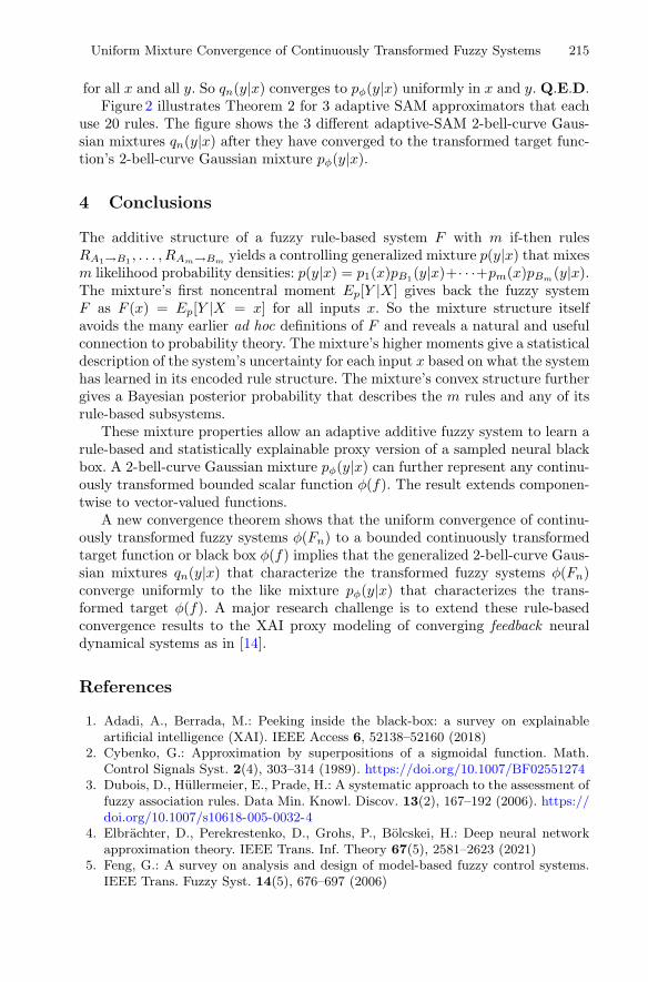
Fig. 1. Gaussian 2-bell-curve mixture representation for the continuously transformedtarget function f(x) = sin(x): φ(f(x)) = sin2(x). The generalized Gaussian mixtureis pφ(y|x) = wφ(x)Nαφ(y|αφ, σ2

α) + (1 − wφ(x))Nβφ(y|βφ, σ2β) from (9) where αφ =

infx∈X φ(f(x)) = 0 and βφ = supx∈X φ(f(x)) = 1. The first panel shows the mixturesurface whose average is sin2(x): Epφ [Y |X = x] = sin2(x). The second panel shows thetwo bell-curve likelihoods centered at αφ and βφ. The purple curve shows the particularGaussian mixture p(y|.51) that results if the input is x = .51.

Figure 1 shows the mixture surface and the two mixed Gaussian bell curvesthat exactly represent the continuously transformed target function φ(f(x)) =

Uniform Mixture Convergence of Continuously Transformed Fuzzy Systems 205

f2(x) = sin2(x) on average. The figure reflects the representation result in The-orem 1. Mixing two normal bell curves gives a generalized probability mix-ture pφ(y|x) such that φ(f(x)) equals the conditional mean Epφ

[Y |X = x]with respect to pφ(y|x) if the function f is bounded and φ is continuous:Epφ

[Y |X = x] = sin2(x). The two mixed likelihood bell curves correspondroughly to the two then-part sets of a two-rule additive fuzzy system. Thisholds exactly when the bell-curve variances converge to zero and thus the nor-mal densities converge to Dirac delta pulses centered at the set centroids. Thislimiting case reflects the older practice of picking then-part sets as spike centeredat centroids.

Figures 2 and 3 illustrate the convergence result in Theorem 2. Figure 3 showsthe mixture surfaces that represent 3 different transformed 20-rule fuzzy systems.Each fuzzy system approximates the transformed target function f2(x) = sin2(x)after the fuzzy systems have converged. The 20 rules RA1→B1 , . . . , RA20→B20

in each system correspond to the 20 mixed likelihood probabilities pBjin each

system’s controlling mixture p(y|x) = p1(x)pB1(y)+ · · ·+p20(x)pB20(y). Figure 2shows what the 2-bell-curve mixture qn(y|x) of each converging fuzzy system Fn

in Fig. 2 looks like after n = 4, 000 epochs of supervised learning. The 3 types ofif-part fuzzy sets require 3 different supervised learning laws [11,16,19]. Figure 4shows the Bayesian rule-posterior histograms for 4 different inputs to the 20-ruleGaussian fuzzy system in Fig. 3.

Figure 5 shows how randomly sampling from the Gaussian fuzzy system’strained 2-bell-curve mixture p(y|x) can reproduce the transformed target func-tion sin2(x) through Monte Carlo averaging. This amounts to drawing a finitenumber of new if-then rules for each input x from a virtual rule continuum [12].The rule histograms in Fig. 4 show that only a few of the stored or virtual rulesfire for a given input x. This helps reduce the sampling costs of Monte Carloaveraging in high dimensions.

The next section presents the basic mathematical facts of the mixture app-roach to rule-based systems.

2 Probability Structure of Additive Fuzzy Rule-BasedSystems

The new mixture convergence theorem exploits the fact that a generalized prob-ability mixture p(y|x) of just two Gaussian bell curves can exactly represent anybounded real function f as the average of the mixture: f(x) = E[Y |X = x] forall x [12,13]. The conditional expectation E[Y |X = x] integrates or sums withrespect to the conditional Gaussian mixture p(y|x):

p(y|x) = w(x)N(y|α, σ2α) + (1 − w(x))N(y|β, σ2

β) (1)

for normal probability density N(y|α, σ2α) with mean or location α and with any

positive variance σ2α > 0 and likewise for N(y|β, σ2

β).The normal densities are likelihoods. The convex mixing weights w(x) and

1 − w(x) are priors or Watkins coefficients [11,26]. The mixing weights depend on

206 B. Kosko

0 1 2 3 4 5 6 7 8x

0

0.2

0.4

0.6

0.8

1

1.2y

y = sin2(x)F20(x)

(a) 20 Sinc rules

0 1 2 3 4 5 6 7 8x

0

0.2

0.4

0.6

0.8

1

1.2

y

y = sin2(x)F20(x)

(b) 20 Gaussian rules

0 1 2 3 4 5 6 7 8x

0

0.2

0.4

0.6

0.8

1

1.2

y

y = sin2(x)F20(x)

(c) 20 Laplacian rules

Fig. 2. Two-bell-curve Gaussian mixture representation of 3 adaptive fuzzy systemsafter they have converged to the sampled continuously transformed bounded targetfunction φ(f(x)) = sin2(x) Each fuzzy approximator used 20 rules but the mixtureplots in panel (b) mixed just two Gaussian bell curves to produce the mixture densityqn(y|x) whose average appears in panel (a). The plots show the mixtures and theiraverages after n = 4, 000 epochs of supervised learning. The convergence plots illustratethe qn(y|x) convergence result in Theorem 2.

the input vector x through the bounded target function f with distinct boundsα ≤ f ≤ β:

w(x) =β − f(x)β − α

. (2)

So the dual mixing weight is 1 − w(x) = f(x)−αβ−α .

The mixture p(y|x) is generalized because it depends on the input x. Ordi-nary mixtures p(y) combine likelihoods that do not depend on x and that haveconstant convex mixing weights that also do not depend on x. The likelihoodscan also depend on x but often do not in practice as we discuss below. The mix-ing weights always depend on x. The 2-bell-curve Gaussian mixture p(y|x) in (1)gives an efficient way to represent a fuzzy or neural approximator and still haveaccess to the mixture’s XAI moment and Bayesian structure [13,20]. Figure 1

Uniform Mixture Convergence of Continuously Transformed Fuzzy Systems 207

shows the mixture representation pφ(y)|x) of the square of the target functionf(x) = sinx. The square-transformed function φ(f) composes the continuoussquare function φ with f to give (φ ◦ f)(x) = φ(f(x)) = sin2 x.

(a) 20 Sinc rules (b) 20 Gaussians rules

(c) 20 Laplacian rules.

Fig. 3. Mixture representations for the 3 adaptive fuzzy approximators φ(Fn) in Fig. 2as they learned the continuously transformed target function φ(f(x)) = sin2(x). Eachfuzzy approximator Fn(x) used 20 rules and so their governing mixtures pn(y|x) eachmixed 20 normal likelihoods with 20 convex mixing weights: pn(y|x) = p1(x)pB1(y) +· · ·+p20(x)pB20(y). The panels show each generalized mixture pn(y|x) after n = 4, 000epochs of learning.

This paper restricts the additive fuzzy systems to the important special caseof SAMs or standard additive model fuzzy systems. Almost all fuzzy systems inpractice are not just additive systems but are SAMs [5,11,18]. Older non-additive(min-max) fuzzy systems [3,23] do not give rise to a rule mixture.

SAMs scale rules to fire them. The input pattern vector x fires a SAM fuzzysystem’s if-then rule RAj→Bj

by scaling the then-part fuzzy set Bj by the degreeaj(x) to which x belongs to the corresponding if-part fuzzy set Aj . The jth ruleRAj→Bj

has the if-part fuzzy set Aj ⊂ Rn with membership or multivalued

indicator function aj : Rn → [0, 1] so that aj(x) = Degree(x ∈ Aj). The rule hasthe corresponding then-part fuzzy set Bj ⊂ R with membership function bj :R → [0, 1]. Then the jth fired then-part set Bj(x) has SAM-scaled membershipfunction bj(y|x) = aj(x)bj(y).

The additive system’s total output set B(y|x) sums and weights the m firedrule then-part sets B1(x), . . . , Bm(x) for respective nonnegative rule weightsw1, . . . , wm. The weights wj may depend on x or on other quantities in someapplications. Then normalized rule firings define a generalized probability mix-ture [12] because we assume that the then-part set functions are nonnegativeand integrable:

208 B. Kosko

p(y|x) =b(y|x)

∫b(y|x)dy

=m∑

j=1

wjaj(x)Vj∑mk=1 wkak(x)Vk

bj(y)Vj

=m∑

j=1

pj(x)pBj(y) (3)

with finite then-part set volume Vj =∫

bj(y|x)dy > 0 and convex mix-ing weights or priors pj(x) = wjaj(x)Vj∑m

k=1 wkak(x)Vk. The SAM rule-firing scaling

bj(y|x) = aj(x)bj(y) gives the likelihood as pBj(y|x) = pBj

(y). Then the fuzzysystem’s output F (x) is just the first noncentral moment of p(y|x) and thus theoutput F (x) is a convex combination of the rule then-part set centroids cj :

F (x) = E[Y |X = x] =∫

y p(y|x) dy =m∑

j=1

pj(x)cj (4)

where cj =∫

ypBj(y)dy. A conditional variance V [Y |X = x] likewise describes

the fuzzy system’s second-order uncertainty for each input x.Figure 3 shows the 3 20-rule mixture surfaces pn(y|x) that encode the squared

target function φ(f(x)) = sin2 x for 3 different adaptive additive fuzzy systemsbased on 3 different types of rule if-part fuzzy sets: sinc, Gaussian, and Laplacianfuzzy sets. Random samples from the target function tune these parametrizedsets along with other rule parameters [11]. The 2-bell-curve mixture compressesthis system information in a multi-rule mixture into a simpler mixture qn(y|x)that can in turn mix with other such mixtures. Figure 2 shows this compressionas the 2-bell-curve representations of the three converging fuzzy systems eachapproach the direct 2-bell-curve representation in Fig. 1.

The fuzzy system’s governing mixture p(y|x) itself states a form of the basictheorem on total probability. So it gives rise at once to a Bayesian posteriordistribution p(j|y, x) over the fuzzy system’s m rules RAj→Bj

:

p(j|y, x) = p(RAj→Bj|y, x) =

pj(x) pBj(y|x)

p(y|x)=

pj(x) pBj(y|x)

∑mk=1 pk(x) pBk

(y|x). (5)

The rule posterior p(j|y, x) gives a complete description of the relative impor-tance of each rule for each input x and observed output value y = F (x). It is apowerful XAI tool that earlier rule-based systems simply ignored. Figure 4 showsthe rule-posterior histograms for the 20-rule Gaussian fuzzy systems in Figs. 2and 3 for 4 different inputs x after n = 4, 000 epochs of supervised learning fromthe target function. This Bayesian posterior description becomes still more pow-erful when an adaptive fuzzy system approximates a neural black box becausethen the rule posterior gives a proxy posterior over the inner workings of theapproximated black box. An additive fuzzy system can uniformly approximateany continuous (or bounded) target function on a compact domain [10,15]. Thisholds in practice if the fuzzy system trains with enough samples from the targetfunction.

The posterior structure holds at a meta level if the fuzzy system F combinesthe rule throughputs of q fuzzy subsystems F 1, . . . , F q. Then the meta-level pos-terior p(k|y, x) describes the relative firing of the q systems for each input x and

Uniform Mixture Convergence of Continuously Transformed Fuzzy Systems 209

1 2 3 4 5 6 7 8 9 10 11 12 13 14 15 16 17 18 19 20Rule index (j)

0

0.2

0.4

0.6

0.8

1

p( j|X

=2.59,Y

=0.75

)

20 Gaussian Rules

1 2 3 4 5 6 7 8 9 10 11 12 13 14 15 16 17 18 19 20Rule index (j)

0

0.2

0.4

0.6

0.8

1

p(j|X

=5 .73

,Y=

− 0.75)

20 Gaussian Rules

(a) (b)

1 2 3 4 5 6 7 8 9 10 11 12 13 14 15 16 17 18 19 20Rule index (j)

0

0.2

0.4

0.6

0.8

1

p( j|X

=6.30

,Y=

0 .0)

20 Gaussian Rules

1 2 3 4 5 6 7 8 9 10 11 12 13 14 15 16 17 18 19 20Rule index (j)

0

0.2

0.4

0.6

0.8

1

p( j| X

=7.36

,Y=

0 .00

)

20 Gaussian Rules

(c) (d)

Fig. 4. Bayesian rule posteriors for the adaptive Gaussian fuzzy system in Figs. 2 and 3.The transformed fuzzy system φ(Fn) at iteration n used Gaussian if-part fuzzy sets forits 20 rules. The panels show the posterior p(j|y, x) after n = 4, 000 epochs of learningfor 4 different input-output pairs (x, y). The posterior histograms show that just onerule contributed the most to the fuzzy system’s rule-interpolated output φ(Fn(x)).Most rules do not fire for a given input.

observed combined output y. The sub-level posterior p(j, k|y, x) describes therelative rule firings of the mk rules in the kth combined fuzzy system F k:

p(j, k|y, x) =pk

j (x)pBkj(y)

∑qk=1

∑mk

j=1 pkj (x)pBk

j(y)

(6)

for the meta-level combined generalized mixture p(y|x):

p(y|x) =q∑

k=1

mk∑

j=1

pkj (x)pBk

j(y). (7)

This telescoping posterior structure holds for any finite number of hierarchicallycombined additive fuzzy systems. Each layer adds another sum to the mixture.

The higher moments of a mixture p(y|x) describe the higher-order statisticalbehavior of the rule-based proxy system. The conditional variance V [Y |X = x]describes the uncertainty of a given output prediction F (x) in terms of theinherent uncertainty in the then-parts of the if-then rules and the extent towhich the output F (x) interpolates over missing rules. The additive structurealso gives a telescoping conditional variance when combining q additive fuzzysystems:

210 B. Kosko

V [Y |X = x] =q∑

k=1

mk∑

j=1

pkj (x)σ2

Bkj

+q∑

k=1

mk∑

j=1

pkj (x)(ck

j − F (x))2 (8)

where σ2Bk

jis the variance of kth SAM’s jth then-part fuzzy set Bk

j . Thesevariance measures can help prune less-certain rules or help prune entire fuzzysubsystems as in random fuzzy foams [20].

A trained mixture p(y|x) also lets one grow a fuzzy system by drawing if-then rules at random from the mixture. This implies sampling from a virtual rulecontinuum to estimate the output F (x) for each input x. Figure 5 shows how suchvirtual rules can estimate the transformed target function sin2 x by Monte Carloaveraging. The mixture becomes a compound in this case because the discreterule index j becomes the continuous index θ [12]: p(y|x) =

∫Θ

pθ(x)pBθ(y)dθ.

The continuous mixture exists so long as either density pθ or pBθis

bounded. This sufficient condition holds because the bound pθ(x) ≤ dimplies pθ(x)pBθ

(y) ≤ pBθ(y)d and because that inequality integrates to∫

Θpθ(x)pBθ

(y)dθ ≤ d for positive constant d since pBθis a density. The fuzzy

system’s output F (x) is again just the realized conditional expectation but withrespect to the rule-continuous mixture p(y|x): F (x) = E[Y |X = x]. So MonteCarlo approximates the output F (x) as it uses the law of large numbers toapproximate the expectation [7]. Each input x requires its own Monte Carlosampling estimate to approximate the output F (x).

Monte Carlo estimation does not depend on the input dimension but it doesconverge slowly [6]. The figure confirms that the standard error in the estimatefalls off with the inverse square root of the number n of samples or rules drawnat random from p(y|x) for a fixed x. So this virtual-rule technique carries a newcomputational burden to estimate F (x). But it can mitigate rule explosion inhigh dimensions and it allows one to work with an estimated mixture p(y|x).

3 Uniform Convergence of Mixtures of TransformedFuzzy Systems

We now show first that a 2-bell-curve Gaussian mixture p(y|x) can exactly rep-resent any continuously transformed bounded real function f for any continuousfunction φ. This result extends the recent result of representing just a boundedtarget function f [13]. We present this and other results only for the scalar-valuedcase even though they extend componentwise to vector-valued systems.

Let f : X → R be any bounded real function. So there exists a constantBf > 0 such that |f(x)| ≤ Bf for all x. Let φ : R → R be any continuous realfunction. The function φ is continuous at each real value x0 just in case for allε > 0 there is a δ = δ(ε, x0) > 0 such that |φ(x0)−φ(x)| < ε if |x0 −x| < δ for allreal x. Define the infimum α = inf f and supremum β = sup f of the boundedfunction f . Assume that f is not constant and so α < β even though the resultsbelow still hold for constant functions if we subtract some constant c > 0 fromα and add it to β. Assume likewise that αφ = inf φ(f) < βφ = supφ(f) in all

Uniform Mixture Convergence of Continuously Transformed Fuzzy Systems 211

0 1 2 3 4 5 6 7 8x

0

0.5

1

1.5

y

y = sin2(x)MC Approximation F100(x)

0 1 2 3 4 5 6 7 8x

0

0.5

1

1.5

y

y = sin2(x)MC Approximation F10,000(x)

(a) 100 samples (b) 10,000 samples

0 1 2 3 4 5 6 7 8x

0

0.5

1

1.5

y

y = sin2(x)MC Approximation F1,000,000(x)

101 102 103 104 105 106

Samples per Monte Carlo estimate

0

0.05

0.1

0.15

0.2

0.25

0.3

MeanSq

uared-Error

(MSE

)(c) 1,000,000 samples (d) Monte Carlo approximation error

Fig. 5. Monte Carlo fuzzy-system approximation of the continuously transformedtarget function φ(f(x)) = sin2(x) for the transformed rule-continuum fuzzy system

φ(F ) based on sampling from the mixture pφ(y|x) = β−φ(f(x))β−α

1√2π

exp[− (y−α)2

2] +

φ(f(x))−αβ−α

1√2π

exp[− (y−β)2

2] if α = infx∈X φ(f(x)) = 0 and β = supx∈X f(x) = 1

and unit variances. The blue lines in panels (a)-(c) show the transformed targetφ(f(x)) = sin2(x). The red lines plot the Monte Carlo estimates of the transformedfuzzy system. Panel (a) plots the sample average of 100 y values drawn at randomfrom [0, 1] for each of 8,000 input values x 0.01 apart. Panel (b) plots the betterapproximation for 10,000 samples at each input x value. Panel (c) plots the still finerapproximation for 1,000,000 such samples. Panel (d) shows the Monte Carlo approx-imation’s slow inverse-square-root decay of the average squared error. Each plottedpoint averaged 10 runs.

the results that follow. The boundedness of f ensures that φ(f) is bounded onthe restricted compact domain [−B,B] since the continuous image of a compactset is itself compact [17] and hence bounded.

Theorem 1 shows how a 2-bell-curve Gaussian mixture pφ(y|x) can exactlyrepresent φ(f) on average for any bounded target function f . It technicallyassumes only that αφ < βφ. It replaces the raw Watkins coefficients w and 1−win (2) with

wφ(x) =βφ − φ(f(x))

βφ − αφ. (9)

with dual convex mixing weight 1 − wφ(x) = φ(f(x))−αφ

βφ−αφ.

212 B. Kosko

Theorem 1: Gaussian Mixture Representation of Continuously Trans-formed Bounded Functions.

Suppose that f : Rn → R is bounded and that αφ = infx∈X φ(f) < βφ =

supx∈X φ(f) for some continuous function φ : R → R. Suppose that the gen-eralized Gaussian mixture density pφ(y|x) mixes two normal probability densityfunctions with Watkins coefficients wφ and 1 − wφ in (9):

pφ(y|x) = wφ(x)Nαφ(y|αφ, σ2

α) + (1 − wφ(x))Nβφ(y|βφ, σ2

β) . (10)

Then pφ(y|x) represents the composite continuous function φ(f) exactly on aver-age: Epφ

[Y |X = x] = φ(f(x)) for all x.

Proof : The centroid of the normal random variable Y ∼ Nαφ(y|αφ, σ2

α) =nαφ

(y) is its location parameter αφ for an positive scale or variance σ2α > 0.

The centroid of nβφ(y) is likewise βφ. Then taking the conditional expectation

with respect to the mixture density pφ(y|x) gives the result:

Eφ[Y |X = x] =∫

y pφ(y|x) dy (11)

= (βφ − φ(f(x))

βφ − αφ)∫

y nαφ(y) dy + (

φ(f(x)) − αφ

βφ − αφ)∫

y nβφ(y) dy

(12)

= (βφ − φ(f(x))

βφ − αφ)αφ + (

φ(f(x)) − αφ

βφ − αφ)βφ (13)

=φ(f(x))[βφ − αφ]

βφ − αφ(14)

= φ(f(x)) (15)

since αφ < βφ. Q.E.D.

We next state and prove two lemmas required to prove the main theorem: the2-bell-curve Gaussian mixtures qn(y|x) that represent continuously transformedapproximators φ(Fn) converge uniformly to the 2-bell-curve mixture pφ(y|x) thatrepresents the transformed target function φ(f). So uniform convergence of thetransformed systems implies uniform convergence of their 2-bell-curve mixtures.

The two lemmas jointly show why we need only assume that the fuzzy approx-imators Fn are individually bounded if they converge uniformly to the targetfunction f . This will imply that the continuously transformed approximatorsφ(Fn) converge uniformly to φ(f). This follows from the result of Lemma 1 thatthe uniform convergence of Fn to f promotes the individual boundedness of eachFn to the much stronger property of uniform boundedness.

Lemma 1: Bounded functions are uniformly bounded if they convergeuniformly.

Suppose that each Fn : Rn → R is bounded and that Fn converges uniformlyto f . Then the functions {Fn} are uniformly bounded and f is bounded.

Proof : Say that Fn is bounded. So there is a bound Bn > 0 such that |Fn(x)| ≤Bn for all x. Suppose that Fn converges uniformly to f . Then for all ε > 0 there

Uniform Mixture Convergence of Continuously Transformed Fuzzy Systems 213

is a positive integer n0 such that for all n ≥ n0: |Fn(x)−f(x)| < ε for all x. Thenwe can bound the tail of the sequence with the triangle inequalities for all n ≥ n0

and for all x: |Fn(x)| − |Fn0(x)| ≤ | |Fn(x)| − |Fn0(x)| | ≤ |Fn(x) − Fn0(x)| ≤|Fn(x) − f(x)| + |f(x) − Fn0(x)| < 2ε from uniform convergence. Take ε = 1

2 forconvenience since ε > 0 was arbitrary. This gives the tail bound: |Fn(x)| < 1 +|Fn0(x)| ≤ 1+Bn0 since Fn0 is bounded. Put B = max(B1, . . . , Bn0−1, 1+Bn0).Then |Fn(x)| ≤ B for all n and all x. So {Fn} is uniformly bounded.

The target function f inherits the boundedness of the functions Fn because ofuniform convergence: |f(x)| = |f(x)−Fn(x)+Fn(x)| ≤ |Fn(x)−f(x)|+|Fn(x)| <12 + B for all x from the uniform boundedness of the sequence {Fn}. Q.E.D.

Lemma 2 uses the crucial real-analytical fact that a continuous function ona compact set is uniformly continuous [17,21]. So then for all ε > 0 there is aδ = δ(ε) > 0 such that |φ(u) − φ(v)| < ε if |u − v| < δ for all u and all v. Theuniform bound B > 0 in Lemma 1 for the functions {Fn} gives the compactinterval [−B,B]. So φ is uniformly continuous on [−B,B]. Then the δ conditionlets the same ε hold for |φ(Fn(x))−φ(f(x))| < ε for all x and thus gives uniformconvergence of φ(Fn) to φ(f). The proof of Theorem 2 shows how this uniformconvergence then leads to the uniform convergence of the 2-bell-curve mixturesqn(y|x) to pφ(y|x).

Lemma 2: Uniform convergence of bounded functions implies uniformconvergence of their continuous transformations.

Suppose that φ : R → R is continuous. Suppose that each Fn : Rn → R isbounded and that Fn converges uniformly to f . Then φ(Fn) converges uniformlyto φ(f).

Proof : Suppose that Fn is bounded and that Fn converges uniformly to f : For allε > 0 there is a positive integer n0 such that for all n ≥ n0: |Fn(x) − f(x)| < ε forall x. Then Lemma 1 states that the sequence {Fn} has the uniform bound B > 0:|Fn(x)| ≤ B for all n and for all x. So −B ≤ Fn(x) ≤ B holds for all positive n.The real interval [−B,B] is compact because it is closed and bounded. Then therestricted continuous function φ : [−B,B] → R on the compact interval [−B,B]is uniformly continuous [17]. So for all ε > 0 there is a δ > 0 that depends only onε and not any x and such that |φ(u) − φ(v)| < ε if |u − v| < δ for all u and for allv in [−B,B]. Put u = Fn(x) and v = f(x). Then |φ(Fn(x)) − φ(f(x))| < ε holdsbecause |Fn(x)− f(x)| = |u− v| < δ. So for every ε > 0 there is a positive integern0 such that for all n ≥ n0: |φ(Fn(x)) − φ(f(x))| < ε for all x. So the compositefunction φ ◦ Fn converges uniformly to the composite function φ ◦ f . Q.E.D.

Theorem 2 uses the 2-bell-curve Gaussian mixture qn(y|x) for each continu-ously transformed fuzzy approximator φ(Fn). Let qn(y|x) denote the 2-bell-curveGaussian mixture for φ(Fn(x)) for fuzzy system Fn with Watkins coefficients vn

and 1 − vn of the transformed system φ(Fn):

vn(x) =βφ − φ(Fn(x))

βφ − αφ(16)

1 − vn(x) =φ(Fn(x)) − βφ

βφ − αφ(17)

214 B. Kosko

such that αφ ≤ φ(Fn) ≤ βφ for all n. Then the 2-bell-curve Gaussian mixtureqn(y|x) has the form

qn(y|x) = vn(x)Nαφ(y|αφ, σ2

α) + (1 − vn(x))Nβφ(y|βφ, σ2

β) . (18)

Theorem 2: Uniform Convergence of Gaussian Mixtures that Repre-sent Continuously Transformed Systems.

Suppose that f : Rn → R is bounded and that αφ = infx∈X φ(f) < βφ =

supx∈X φ(f) for some continuous function φ : R → R and that αφ ≤ φ(Fn(x)) ≤βφ for all n and for all x. Suppose that the bounded additive fuzzy systems Fn

uniformly converge to the target function f . Suppose that the 2-bell-curve Gaus-sian mixture density pφ(y|x) that represents φ(f) mixes two normal probabilitydensity functions with Watkins coefficients wφ and 1 − wφ in (9):

pφ(y|x) = wφ(x)Nαφ(y|αφ, σ2

α) + (1 − wφ(x))Nβφ(y|βφ, σ2

β) . (19)

Suppose further that the Gaussian mixture qn(y|x) with Watkins coefficients vn

and 1 − vn in (16)–(17) that represents φ(Fn) has the like 2-bell-curve form

qn(y|x) = qn(x)Nαφ(y|αφ, σ2

α) + (1 − vn(x))Nβφ(y|βφ, σ2

β) . (20)

Then qn(y|x) converges uniformly to pφ(y|x) uniformly in x and y.

Proof : The two normal bell-curve likelihoods Nαφ(y|αφ, σ2

α) and Nβφ(y|βφ, σ2

β)are bounded functions for any fixed variances σ2

α > 0 and σ2β > 0. So |nαφ

(y) −nβφ

(y)| ≤ max(nαφ(αφ), nβφ

(βφ)) holds for all y values for the modes αφ andβφ. Then |nα(y) − nβ(y)| < D if D = max(nα(α), nβ(β)) + 1.

Lemmas 1 and 2 and the boundedness of Fn imply that φ(Fn) convergesuniformly to φ(f) because φ is continuous and because Fn converges uniformlyto f . So for all ε > 0 there is a positive integer n0 such that for all integersn ≥ n0: |φ(Fn(x)) − φ(f(x))| <

βφ−αφ

D ε for all x ∈ X. Then using the Watkinscoefficients wφ and vn for the two respective Gaussian mixtures pφ(y|x) andqφ(y|x) gives for n ≥ n0:

|qn(y|x)− pφ(y|x)| =1

βφ − αφ|(βφ − φ(Fn(x)))nαφ (y) + (φ(Fn(x))− αφ)nβφ

(y)

− (βφ − φ(f(x)))nαφ (y)− (φ(f(x))− αφ)nβφ(y)| (21)

=1

βφ − αφ|φ(Fn(x))(nβφ

(y)− nαφ (y))− φ(f(x))(nβφ(y)− nαφ (y))|

(22)

=1

βφ − αφ|φ(Fn(x))− φ(f(x))||nαφ (y)− nβφ

(y)| (23)

<1

βφ − αφ|φ(Fn(x))− φ(f(x))| D (24)

<1

βφ − αφ

βφ − αφ

Dε D (25)

= ε (26)

Uniform Mixture Convergence of Continuously Transformed Fuzzy Systems 215

for all x and all y. So qn(y|x) converges to pφ(y|x) uniformly in x and y. Q.E.D.Figure 2 illustrates Theorem 2 for 3 adaptive SAM approximators that each

use 20 rules. The figure shows the 3 different adaptive-SAM 2-bell-curve Gaus-sian mixtures qn(y|x) after they have converged to the transformed target func-tion’s 2-bell-curve Gaussian mixture pφ(y|x).

4 Conclusions

The additive structure of a fuzzy rule-based system F with m if-then rulesRA1→B1 , . . . , RAm→Bm

yields a controlling generalized mixture p(y|x) that mixesm likelihood probability densities: p(y|x) = p1(x)pB1(y|x)+· · ·+pm(x)pBm

(y|x).The mixture’s first noncentral moment Ep[Y |X] gives back the fuzzy systemF as F (x) = Ep[Y |X = x] for all inputs x. So the mixture structure itselfavoids the many earlier ad hoc definitions of F and reveals a natural and usefulconnection to probability theory. The mixture’s higher moments give a statisticaldescription of the system’s uncertainty for each input x based on what the systemhas learned in its encoded rule structure. The mixture’s convex structure furthergives a Bayesian posterior probability that describes the m rules and any of itsrule-based subsystems.

These mixture properties allow an adaptive additive fuzzy system to learn arule-based and statistically explainable proxy version of a sampled neural blackbox. A 2-bell-curve Gaussian mixture pφ(y|x) can further represent any continu-ously transformed bounded scalar function φ(f). The result extends componen-twise to vector-valued functions.

A new convergence theorem shows that the uniform convergence of continu-ously transformed fuzzy systems φ(Fn) to a bounded continuously transformedtarget function or black box φ(f) implies that the generalized 2-bell-curve Gaus-sian mixtures qn(y|x) that characterize the transformed fuzzy systems φ(Fn)converge uniformly to the like mixture pφ(y|x) that characterizes the trans-formed target φ(f). A major research challenge is to extend these rule-basedconvergence results to the XAI proxy modeling of converging feedback neuraldynamical systems as in [14].

References

1. Adadi, A., Berrada, M.: Peeking inside the black-box: a survey on explainableartificial intelligence (XAI). IEEE Access 6, 52138–52160 (2018)

2. Cybenko, G.: Approximation by superpositions of a sigmoidal function. Math.Control Signals Syst. 2(4), 303–314 (1989). https://doi.org/10.1007/BF02551274

3. Dubois, D., Hullermeier, E., Prade, H.: A systematic approach to the assessment offuzzy association rules. Data Min. Knowl. Discov. 13(2), 167–192 (2006). https://doi.org/10.1007/s10618-005-0032-4

4. Elbrachter, D., Perekrestenko, D., Grohs, P., Bolcskei, H.: Deep neural networkapproximation theory. IEEE Trans. Inf. Theory 67(5), 2581–2623 (2021)

5. Feng, G.: A survey on analysis and design of model-based fuzzy control systems.IEEE Trans. Fuzzy Syst. 14(5), 676–697 (2006)

216 B. Kosko

6. Glasserman, P.: Monte Carlo Methods in Financial Engineering, vol. 53. Springer,Heidelberg (2013). https://doi.org/10.1007/978-0-387-21617-1

7. Hogg, R.V., McKean, J., Craig, A.T.: Introduction to Mathematical Statistics.Pearson, London (2013)

8. Hornik, K., Stinchcombe, M., White, H.: Multilayer feedforward networks are uni-versal approximators. Neural Netw. 2(5), 359–366 (1989)

9. Kosko, B.: Neural Networks and Fuzzy Systems. Prentice-Hall, Hoboken (1991)10. Kosko, B.: Fuzzy systems as universal approximators. IEEE Trans. Comput.

43(11), 1329–1333 (1994)11. Kosko, B.: Fuzzy Engineering. Prentice-Hall, Hoboken (1996)12. Kosko, B.: Additive fuzzy systems: from generalized mixtures to rule continua. Int.

J. Intell. Syst. 33(8), 1573–1623 (2018)13. Kosko, B.: Convergence of generalized probability mixtures that describe adap-

tive fuzzy rule-based systems. In: 2020 IEEE International Conference on FuzzySystems (FUZZ-IEEE), pp. 1–8. IEEE (2020)

14. Kosko, B.: Bidirectional associative memories: unsupervised Hebbian learning tobidirectional backpropagation. IEEE Trans. Syst. Man Cybern. Syst. 51(1), 103–115 (2021)

15. Kreinovich, V., Mouzouris, G.C., Nguyen, H.T.: Fuzzy rule based modeling as auniversal approximation tool. In: Nguyen, H.T., Sugeno, M. (eds.) Fuzzy Systems.The Springer Handbook Series on Fuzzy Sets, vol. 2, pp. 135–195. Springer, Boston(1998). https://doi.org/10.1007/978-1-4615-5505-6 5

16. Mitaim, S., Kosko, B.: The shape of fuzzy sets in adaptive function approximation.IEEE Trans. Fuzzy Syst. 9(4), 637–656 (2001)

17. Munkres, J.: Topology (2014)18. Nguyen, A.-T., Taniguchi, T., Eciolaza, L., Campos, V., Palhares, R., Sugeno, M.:

Fuzzy control systems: past, present and future. IEEE Comput. Intell. Mag. 14(1),56–68 (2019)

19. Osoba, O., Mitaim, S., Kosko, B.: Bayesian inference with adaptive fuzzy priorsand likelihoods. IEEE Trans. Syst. Man Cybern. Part B: Cybern. 41(5), 1183–1197(2011)

20. Panda, A.K., Kosko, B.: Random fuzzy-rule foams for explainable AI. In: FuzzyInformation Processing 2020, Proceedings of NAFIPS-2020. Springer, Heidelberg(2020). https://doi.org/10.1007/978-3-030-71098-9

21. Rudin, W.: Real and Complex Analysis. McGraw-Hill Education, New York (2006)22. Samek, W., Montavon, G., Vedaldi, A., Hansen, L.K., Muller, K.-R. (eds.): Explain-

able AI: Interpreting, Explaining and Visualizing Deep Learning. LNCS (LNAI),vol. 11700. Springer, Cham (2019). https://doi.org/10.1007/978-3-030-28954-6

23. Terano, T., Asai, K., Sugeno, M.: Fuzzy Systems Theory and its Applications.Academic Press Professional Inc., Cambridge (1992)

24. Tjoa, E., Guan, C.: A survey on explainable artificial intelligence (XAI): towardmedical XAI. IEEE Trans. Neural Netw. Learn. Syst. pp. 1–21 (2020). https://doi.org/10.1109/TNNLS.2020.3027314

25. van der Waa, J., Nieuwburg, E., Cremers, A., Neerincx, M.: Evaluating XAI: a com-parison of rule-based and example-based explanations. Artif. Intell. 291, 103404(2021)

26. Watkins, F.: The representation problem for additive fuzzy systems. In: Proceed-ings of the International Conference on Fuzzy Systems (IEEE FUZZ-1995), pp.117–122 (1995)