Uniformly Valid Multiple Spatial-Temporal Scale …jfish/Unif_Valid.pdf1 Uniformly Valid Multiple Spatial-Temporal Scale Modeling for Wave Propagation in Heterogeneous Media Jacob

1

Uniformly Valid Multiple Spatial-Temporal Scale Modeling for Wave Propagation in Heterogeneous Media

Jacob Fish and Wen ChenDepartment of Civil Engineering and Scientific Computation Research Center,

Rensselaer Polytechnic Institute, Troy, NY 12180, USA

Abstract: A novel dispersive model for wave propagation in heterogeneous media is developed. Themethod is based on a higher-order mathematical homogenization theory with multiple spatial and temporalscales. By this approach a fast spatial scale and a series of slow temporal scales are introduced to account forrapid spatial fluctuations of material properties as well as for the long-term behavior of the homogenizedsolution. The problem of secularity arising from the classical multiple spatial scale homogenization theoryfor wave propagation problems is resolved, giving rise to uniformly valid dispersive model. The proposeddispersive model is solved analytically and its solution has be found to be in good agreement with thenumerical solution of the source problem in a heterogeneous medium.

1. Introduction When a wavelength of a traveling signal in a heterogeneous medium is comparable tothe characteristic length of the microstructure, successive reflection and refraction of thewaves between the interfaces of the material lead to significant dispersion effects (see forexample [1][2][3]). The interest on the subject matter stems from the fact that the phenom-enon of dispersion cannot be captured by the classical homogenization theory.

The use of multiple-scale expansions as a systematic tool of homogenization for prob-lems other than elastodynamics can be traced to Sanchez-Palencia [4], Benssousan, Lionsand Papanicoulau [5], and Bakhvalov and Panasenko [6]. The role of higher order terms inthe asymptotic expansion has been investigated in statics by Gambin and Kroner [7], andBoutin [8]. In elastodynamics, Boutin and Auriault [9] demonstrated that the terms of ahigher order successively introduce effects of polarization, dispersion and attenuation.

For wave propagation in heterogeneous media, a single-frequency time dependence istypically assumed [10]. Notable exceptions are the recent articles of Fish and Chen[11][12], which investigated the initial-boundary value problem with rapidly varying coef-ficients. In [11] it has been shown that while higher-order multiple scale expansion inspace is capable of capturing the dispersion effect when the temporal scale of observationis small, it introduces secular terms which grow unbounded with time. In [12], a slow tem-poral scale was introduced to eliminated the secular terms up to the second order and tocapture the long-term behavior of the homogenized solution.

In an attempt to develop a uniformly valid dispersive model up to an arbitrary order, weextend the theory developed in [12] to fast spatial and a series of slow temporal scales.The fast spatial scale is designated to account for rapid spatial fluctuations of materialproperties and a series of slow temporal scales are aimed at capturing the long-term evolu-tion of the homogenization solutions. This results in a dispersive uniformly valid model,solution of which is obtained analytically and subsequently validated against the numeri-cal solution of the source problem in a heterogeneous medium.

2

2. Problem Statement

We consider wave propagation normal to layers of an array of elastic bilaminates in a

periodic arrangement with as a characteristic length as shown in Figure 1. The govern-ing elastodynamics equation of is given by

(1)

with appropriate boundary and initial conditions

, (2)

where denotes the displacement field; and the mass density and

elastic modulus, respectively; and denote the differentiation with respect to x

and time respectively; and in (1) denotes a rapid spatial variation of materialproperties.

The goal is to establish an effective homogeneous model in which local fluctuations intro-duced by material heterogeneity do not appear explicitly and the response of a heteroge-neous medium can be approximated by the response of the effective homogeneousmedium. This is facilitated by the method of multiple scale asymptotic expansion in spaceand time.

3. Asymptotic Analysis with Multiple Spatial and Temporal Scales

Under the premise that the macro domain is much larger than the unit cell

domain , i.e. , it is convenient to introduce a microscopicspatial length variable y [9][16] such that

(3)

where , and c are the macroscopic wavelength, the circular frequency, the wavenumber and the phase velocity of the macroscopic wave, respectively. In addition to thisfast spatial variable, we introduce multiple time scales

Ω

ρ x ε⁄( )u tt; E x ε⁄( )u x; x;

– 0=

u x 0,( ) f x( )= u t; x 0,( ) q x( )=

u x t,( ) ρ x ε⁄( ) E x ε⁄( )( ) x; ( ) t;

0 ε 1«<

Figure 1: A bilaminate with a periodic microstructure

L λ 2π( )⁄=

Ω Ω L⁄ ωΩ( ) c⁄ kΩ 1«= =

y x ε⁄=

λ ω k,

3

, (4)

where is the usual time coordinate and , k > 0 are various slow time scales. Since the

response quantities u and depend on x, , , , and , a multiple-scale

asymptotic expansion is employed to approximate the displacement and stress fields

,

(5)

Homogenization process consists of inserting the asymptotic expansions (5) into thegoverning equation (1), identifying the terms with the equal power of , and then solvingthe resulting problems.

Following the aforementioned procedure and expressing the spatial and temporal deriv-atives in terms of the fast and slow space-time coordinates

(6)

(7)

we obtain a series of equations in ascending power of starting with .

3.1 Homogenization

At , we have

(8)

The general solution of (8) is

(9)

where and are functions of macro coordinates and

multiple temporal scales. To ensure periodicity of over the unit cell domain

in the stretched coordinate system y, must vanish, implying that the leading-order dis-

placement depends only on the macroscale

(10)

tk ε2kt= k 0 1 2 … m, , , ,=( )

t0 tkσ y x ε⁄= t0 t1 … tm

u x y t0 t1 … tm, , , , ,( ) εiui x y t0 t1 … tm, , , , ,( )

i 0=

nn

∑=

σ x y t0 t1 … tm, , , , ,( ) εiσi x y t0 t1 … tm, , , , ,( )i 1–=

nn

∑=

ε

u x; u x, ε 1–u y,+=

u t; u t0, ε2u t1, ε4

u t2, … ε2mu tm,+ + + +=

ε ε 2–

O 1( )

O ε 2–( )

E y( )u0 y, y,

0=

u0 a1 x t0 t1 … tm, , , ,( ) 1E y( )----------- y a2 x t0 t1 … tm, , , ,( )+d

y0

y0 y+

∫=

a1 x t0 t1 … tm, , , ,( ) a2 x t0 t1 … tm, , , ,( )

u0 Ωˆ

Ω ε⁄=

a1

u0 u0 x t0 t1 … tm, , , ,( )=

4

At order , the perturbation equation is

(11)

Due to linearity of the above equation, the general solution of is

(12)

Substituting (12) into (11) yields

(13)

For a -periodic function , we define an averaging operator

(14)

The boundary conditions for the unit cell problem described by (13) are

(a) Periodicity: ,

(b) Continuity: ,

(c) Normalization: (15)

where is the volume fraction of the unit cell; is the jump operator; and

, (16)

Equation (13) together with the boundary conditions (15) define the unit cell boundaryvalue problem from which can be uniquely determined as

, (17)

At , the perturbation equation is

(18)

Applying the averaging operator defined in (14) to the above equation and taking intoaccount periodicity of , we get the macroscopic equation of motion at :

O ε 1–( )

E y( ) u0 x, u1 y,+( ) y, 0=

u1

u1 x y t0 t1 … tm, , , , ,( ) U1 x t0 t1 … tm, , , ,( ) L y( )u0 x,+=

E y( ) 1 L y,+( ) y, 0=

Ωˆ

g x y t0 t1 … tm, , , , ,( )

g⟨ ⟩ 1

Ωˆ------- g x y t0 t1 … tm, , , , ,( ) yd

Ω

∫=

u1 y 0=( ) u1 y Ωˆ

=( )= σ0 y 0=( ) σ0 y Ωˆ

=( )=

u1 y αΩˆ

=( ) 0= σ0 y αΩˆ

=( ) 0=

u1 x y t0 t1 … tm, , , , ,( )⟨ ⟩ U1 x t0 t1 … tm, , , ,( )= ⇒ L y( )⟨ ⟩ 0=

0 α 1≤ ≤

σi E y( ) ui x, ui 1 y,++( )= i 0 1 … nn, , ,=

L y( )

L1 y( )1 α–( ) E2 E1–( )1 α–( )E1 αE2+

----------------------------------------- yαΩ

ˆ

2--------–= L2 y( )

α E1 E2–( )1 α–( )E1 αE2+

---------------------------------------- y1 α+( )Ω

ˆ

2-----------------------–=

O 1( )

ρ y( )u0 t0t0, E y( ) u0 x, u1 y,+( ) x,– E y( ) u1 x, u2 y,+( ) y,– 0=

σ1 O 1( )

5

(19)

where

, (20)

The above macroscopic equation of motion is non-dispersive. In order to capture disper-sion effects, we next consider higher-order equilibrium equations.

3.2 Homogenization

is determined from perturbation equation (18). Substituting (12) and (19) into

(18), yields

(21)

where

(22)

We seek for the solution of in the form of

(23)


(24)

The boundary conditions for the above equation are: periodicity and continuity of

and as well as the normalization condition . Once the solution of is

obtained it can be easily verified that satisfies

, (25)

Consider the equilibrium equation:

(26)

Applying the averaging operator to the above equation, and exploiting (25) together withperiodicity of yields

(27)

3.3 Homogenization

ρ0u0 t0t0, E0u0 xx,– 0=

ρ0 ρ⟨ ⟩ αρ1 1 α–( )ρ2+= = E0 E y( ) 1 L y,+( )⟨ ⟩E1E2

1 α–( )E1 αE2+----------------------------------------= =

O ε( )

u2 O 1( )

E y( )u2 y, y, E0 θ y( ) 1–( ) E y( )L( ) y,– u0 xx, E y( )U1 x,

y,–=

θ y( ) ρ y( ) ρ0⁄=

u2

u2 x y t0 t1 … tm, , , , ,( ) U2 x t0 t1 … tm, , , ,( ) L y( )U1 x, M y( )u0 xx,+ +=

E y( ) L M y,+( ) y, E0 θ y( ) 1–( )=

u2

σ1 M y( )⟨ ⟩ 0= M y( )

M y( )

ρL⟨ ⟩ 0= E L M y,+( )⟨ ⟩ 0=

O ε( )

ρ y( )u1 t0t0, E y( ) u1 x, u2 y,+( ) x,

– E y( ) u2 x, u3 y,+( ) y,

– 0=

σ2

ρ0U1 t0t0, E0U1 xx,– 0=

O ε2( )

6

is determined from the perturbation equation (26). Inserting (12) and (23) into

(26) and making use of the macroscopic equations of motion (19) and (27), gives

(28)

Due to linearity of (28) the general solution of is as follows:

(29)

Substituting (29) into (28) gives

(30)

The above equation, together with the periodicity and continuity of and as well as

the normalization condition , fully determine . After is solved for,we can calculate

(31)

(32)

Consider the equilibrium equation of :

(33)

Applying the averaging operator to the above equation, and exploiting periodicity of

and making use of (31) and (32) leads to

(34)

where

(35)

u3 O ε( )

E y( )u3 y, y, E0θ y( )L E y( ) L M y,+( )– E y( )M( ) y,– u0 xxx, +=

E0 θ y( ) 1–( ) E y( )L( ) y,– U1 xx, E y( )U2 x, y,–

u3

u3 x y t0 t1 … tm, , , , ,( ) U3 x t0 t1 … tm, , , ,( ) L y( )U2 x,+ +=

M y( )U1 xx, N y( )u0 xxx,+

E y( ) M N y,+( ) y, E0Lθ y( ) E y( ) L M y,+( )–=

u3 σ2

N y( )⟨ ⟩ 0= N y( ) N y( )

ρM⟨ ⟩α 1 α–( )[ ]2 ρ2 ρ1–( ) E1ρ1 E2ρ2–( )E0Ω

ˆ 2

12ρ0E1E2-----------------------------------------------------------------------------------------------------=

E M Ny,+( )⟨ ⟩α 1 α–( )E0Ω

ˆ 2

12ρ0-----------------------------------

E2 E1–( ) α2ρ1 1 α–( )2ρ2–[ ] E0ρ0+

1 α–( )E1 αE2+------------------------------------------------------------------------------------------- ρ0–

–=

O ε2( )

ρ y( ) u2 t0t0, 2u0 t0t1,+( ) E y( ) u2 x, u3 y,+( ) x,– E y( ) u3 x, u4 y,+( ) y,– 0=

σ3

ρ0U2 t0t0, E0U2 xx,–1

ε2-----Edu0 xxxx, 2ρ0u0 t0t1,–=

Ed

α 1 α–( )[ ]2E1ρ1 E2ρ2–( )2

E0Ω2

12ρ02 1 α–( )E1 αE2+[ ]2

---------------------------------------------------------------------------------=

7

characterizes the effect of the microstructure on the macroscopic behavior. It is pro-

portional to the square of the dimension of the unit cell . Note that for homogeneous

materials (i.e., or ) and in the case of impedance ratio

( ) equal to unity, vanishes.

3.4 Homogenization

is determined from perturbation equation (33). Substituting (12), (23) and

(29) into (33) and making use of (19), (27) and (34) yields

(36)

Due to linearity, the general solution of can be sought in the form

(37)


(38)


the normalization condition , uniquely determines . The solution of

satisfies

, (39)

The equilibrium equation at is:

(40)

Applying the averaging operator to (40), exploiting periodicity of and making use of

(39) yields

(41)

Ed

Ωα 0= α 1= r z2 z1⁄=

z Eρ= Ed

O ε3( )

u4 O ε2( )

E y( )u4 y, y, θ y( ) E0M Ed ε2⁄+( ) E y( ) M N y,+( )– E y( )N( ) y,– u0 xxxx, +=

E0θ y( )L E y( ) L M y,+( )– E y( )M( ) y,– U1 xxx, +

E0 θ y( ) 1–( ) E y( )L( ) y,– U2 xx, E y( )U3 x, y,

–

u4


M y( )U2 xx, N y( )U1 xxx, P y( )u0 xxxx,+ +

E y( ) N Py,+( ) y, θ y( ) E0M Ed ε2⁄+( ) E y( ) M N y,+( )–=

u4 σ3

P y( )⟨ ⟩ 0= P y( )P y( )

ρN⟨ ⟩ 0= E N Py,+( )⟨ ⟩ 0=

O ε3( )

ρ y( ) u3 t0t0, 2u1 t0t1,+( ) E y( ) u3 x, u4 y,+( ) x,– E y( ) u4 x, u5 y,+( ) y,– 0=

σ4

ρ0U3 t0t0, E0U3 xx,–1

ε2-----EdU1 xxxx, 2ρ0U1 t0t1,–=

8

3.5 Homogenization

is determined from perturbation equation (40). Substituting (12), (23), (29)

and (37) into (40) and making use of (19), (27), (34) and (41) yields

(42)

Due to linearity, the general solution of can be sought in the form

(43)

Substituting (43) into (42) gives

(44)


the normalization condition , uniquely determines . After is

solved for, expressions for and can be derived.

The equilibrium equation is:

(45)

Applying the averaging operator to the above equation and taking into account periodic-ity of , gives

(46)

where

O ε4( )

u5 O ε3( )

E y( )u5 y, y, θ y( ) E0N LEd ε2⁄+( ) E y( ) N Py,+( )– E y( )P( ) y,– u0 xxxxx, +=

θ y( ) E0M Ed ε2⁄+( ) E y( ) M N y,+( )– E y( )N( ) y,– U1 xxxx, +

E0θ y( )L E y( ) L M y,+( )– E y( )M( ) y,– U2 xxx, +


u5


M y( )U3 xx, N y( )U2 xxx, P y( )U1 xxxx, Q y( )u0 xxxxx,+ + +

E y( ) P Qy,+( ) y, θ y( ) E0N LEd ε2⁄+( ) E y( ) N Py,+( )–=

u5 σ4

Q y( )⟨ ⟩ 0= Q y( ) Q y( )ρP⟨ ⟩ E P Qy,+( )⟨ ⟩

O ε4( )

ρ y( ) u4 t0t0, 2u2 t0t1, 2u0 t0t2, u0 t1t1,+ + +( ) E y( ) u4 x, u5 y,+( ) x,– –

E y( ) u5 x, u6 y,+( ) y, 0=

σ5

ρ0t02

2

∂

∂ U4 E0x

2

2

∂

∂ U4–Ed

ε2------

x4

4

∂

∂ U2 Eg

ε4------

x6

6

∂

∂ u0 2ρ0 t0 t∂ 1

2

∂∂ U2 2ρ0 t0 t2∂

2

∂∂ u0– ρ0

t12

2

∂

∂ u0–––=

9

(47)

3.6 Homogenization

Next we determine the value of from perturbation equation (45). Substituting

(12), (23), (29), (37) and (43) into (45) and making use of (19), (27), (34), (41) and (46),yields

(48)

Due to linearity of (48) the general solution of can be sought in the form

(49)

Substituting the above expression into (48) yields

(50)


the normalization condition , uniquely determines . After issolved for, it can be easily shown that

, (51)

The equilibrium equation at is:

Eg

α 1 α–( )[ ]2E1ρ1 E2ρ2–( )2

E0Ω4

360ρ04 1 α–( )E1 αE2+[ ]4

--------------------------------------------------------------------------------- α2E2

2 2α2ρ12 1 α–( )2ρ2

2– +[=

6α 1 α–( )ρ1ρ2 ] 2+ α 1 α–( )E1E2 3α2ρ12 3 1 α–( )2ρ2

2+ +[

11α 1 α–( )ρ1ρ2] 1 α–( )2E1

2 α2ρ12

2 1 α–( )2ρ22

6α 1 α–( )ρ1ρ2 ] ––[–

O ε5( )

u6 O ε4( )

E y( )u6 y, y, θ y( ) E0P MEd ε2Eg ε4⁄–⁄+( ) E y( ) P Qy,+( )– –=

E y( )Q( ) y, u0 xxxxxx, θ y( ) E0N LEd ε2⁄+( ) E y( ) N Py,+( )– –+

E y( )P( ) y, U1 xxxxx, θ y( ) E0M Ed ε2⁄+( ) E y( ) M N y,+( ) ––+

E y( )N( ) y, U2 xxxx, E0θ y( )L E y( ) L M y,+( )– E y( )M( ) y,– U3 xxx,+ +


u6


M y( )U4 xx, N y( )U3 xxx, P y( )U2 xxxx, Q y( )U1 xxxxx, R y( )u0 xxxxxx,+ + + +

E y( ) Q Ry,+( ) y, θ y( ) E0P MEd ε2⁄ Eg ε4⁄–+( ) E y( ) P Qy,+( )–=

u6 σ5

R y( )⟨ ⟩ 0= R y( ) R y( )

ρQ⟨ ⟩ 0= E Q Ry,+( )⟨ ⟩ 0=

O ε5( )

10

(52)

Applying the averaging operator to the above equation, exploiting periodicity of and

making use of (51) yields

(53)

3.7 Higher Order Homogenization and Summary of Macroscopic Equations

The homogenization process described in the previous section can be systematicallygeneralized to an arbitrary order. In this section we summarize various order macroscopicequations of motion and state the initial and boundary conditions.

The macroscopic equations of motion are:

: (19)

: (27)

: (34)

: (41)

: (46)

: (53)

and higher:

ρ y( ) u5 t0t0, 2u3 t0t1, 2u1 t0t2, u1 t1t1,+ + +( ) E y( ) u5 x, u6 y,+( ) x,

– –

E y( ) u6 x, u7 y,+( ) y,

0=

σ6

ρ0t02

2

∂

∂ U5 E0x

2

2

∂

∂ U5–Ed

ε2------

x4

4

∂

∂ U3 Eg

ε4------

x6

6

∂

∂ U1 2ρ0 t0 t1∂

2

∂∂ U3 2ρ0 t0 t2∂

2

∂∂ U1– ρ0

t12

2

∂

∂ U1–––=

O 1( ) ρ0u0 t0t0, E0u0 xx,– 0=

O ε( ) ρ0U1 t0t0, E0U1 xx,– 0=

O ε2( ) ρ0U2 t0t0, E0U2 xx,–1

ε2-----Edu0 xxxx, 2ρ0u0 t0t1,–=

O ε3( ) ρ0U3 t0t0, E0U3 xx,–1

ε2-----EdU1 xxxx, 2ρ0U1 t0t1,–=

O ε4( ) ρ0t02

2

∂

∂ U4 E0x

2

2

∂

∂ U4–Ed

ε2------

x4

4

∂

∂ U2 Eg

ε4------

x6

6

∂

∂ u0 2ρ0 t0 t1∂

2

∂∂ U2 2ρ0 t0 t∂ 2

2

∂∂ u0– ρ0

t12

2

∂

∂ u0–––=

O ε5( ) ρ0t02

2

∂

∂ U5 E0x

2

2

∂

∂ U5–Ed

ε2------

x4

4

∂

∂ U3 Eg

ε4------

x6

6

∂

∂ U1 2ρ0 t0 t1∂

2

∂∂ U3 2ρ0 t0 t∂ 2

2

∂∂ U1– ρ0

t12

2

∂

∂ U1–––=

O ε6( )

ρ0t02

2

∂

∂ U2m E0x

2

2

∂

∂ U2m–Ed

ε2------

x4

4

∂

∂ U2 m 1–( ) Eg

ε4------

x6

6

∂

∂ U2 m 2–( )– +=

11

(54)

(55)

where ; ; , , , can be evaluated

using higher-order homogenization process.

Subsequently, we consider the following model problem: a domain composed of anarray of bilaminates with fixed boundary at and free boundary at subjected

Es1

ε6--------

x8

8

∂

∂ U2 m 3–( ) Es2

ε8--------

x10

10

∂

∂ U2 m 4–( )– … 1–( )m 1+ Es m 2–( )

ε2m-------------------

x2 m 1+( )

2 m 1+( )

∂

∂ u0 –+ +

2ρ0 t0 tm∂

2

∂∂ u0

t1 tm 1–∂

2

∂∂ u0 … 1

2---

tm 2⁄2

2

∂

∂ u0+ + +

–

2ρ0 t0 tm 1–∂

2

∂∂ U2

t1 tm 2–∂

2

∂∂ U2 … 1

2---

t m 1–( ) 2⁄2

2

∂

∂ U2+ + +

–

2ρ0 t0 tm 2–∂

2

∂∂ U4

t1 tm 3–∂

2

∂∂ U4 … 1

2---

t m 2–( ) 2⁄2

2

∂

∂ U4+ + +

… 2ρ0 t0 t1∂

2

∂∂ U2 m 1–( )––

ρ0t02

2

∂

∂ U2m 1+ E0x

2

2

∂

∂ U2m 1+–Ed

ε2------

x4

4

∂

∂ U2m 1– Eg

ε4------

x6

6

∂

∂ U2m 3–– +=

Es1

ε6--------

x8

8

∂

∂ U2m 5– Es2

ε8--------

x10

10

∂

∂ U2m 7–– … 1–( )m 1+ Es m 2–( )

ε2m-------------------

x2 m 1+( )

2 m 1+( )

∂

∂ U1 –+ +

2ρ0 t0 tm∂

2

∂∂ U1

t1 tm 1–∂

2

∂∂ U1 … 1

2---

tm 2⁄2

2

∂

∂ U1+ + +

–

2ρ0 t0 tm 1–∂

2

∂∂ U3

t1 tm 2–∂

2

∂∂ U3 … 1

2---

t m 1–( ) 2⁄2

2

∂

∂ U3+ + +

–

2ρ0 t0 tm 2–∂

2

∂∂ U5

t1 tm 3–∂

2

∂∂ U5 … 1

2---

t m 2–( ) 2⁄2

2

∂

∂ U5+ + +

… 2ρ0 t0 t1∂

2

∂∂ U2m 1–––

m 3 4 5 …, , ,= tk k 0 1 2 … m, , , ,=( ) Es1 Es2 … Es m 2–( )

x 0= x l=

12

to an initial disturbance in the displacement field. At , the displacement field isdetermined by the equation of motion (19) and the following initial and boundary condi-tions

ICs: , (56)

BCs: , (57)

The calculation of is obtained by solving the equation of motion

(27). The initial and boundary conditions applied to must be such that the global field

meets macroscopic initial conditions and conditions imposed on the boundary:

Taking into account (56) and (57), the initial and boundary conditions for become

ICs: ,

BCs: ,

Similarly, the macroscopic field is determined from the equation

of motion (34), with the initial and boundary conditions for such that the global

field should satisfy the macroscopic initial and boundary conditions.

With this in mind, we obtain the initial and boundary conditions for different order equa-tions of motion:

ICs: ,

, (58)

BCs: , (59)

From the above equations of motion and the initial-boundary conditions, we can readilydeduce that

f x( ) O 1( )

u0 x 0 0 … 0, , , ,( ) f x( )= u0 t; x 0 0 … 0, , , ,( ) q x( ) 0= =

u0 0 t0 t1 … tm, , , ,( ) 0= u0 x, l t0 t1 … tm, , , ,( ) 0=

εU1 x t0 t1 … tm, , , ,( )

εU1

u0 εU1+

u0 x 0 0 … 0, , , ,( ) εU1 x 0 0 … 0, , , ,( )+ f x( )=

u0 t; x 0 0 … 0, , , ,( ) εU1 t; x 0 0 … 0, , , ,( )+ 0=

u0 0 t0 t1 … tm, , , ,( ) εU1 0 t0 t1 … tm, , , ,( )+ 0=

u0 x, l t0 t1 … tm, , , ,( ) εU1 x, l t0 t1 … tm, , , ,( )+ 0=

εU1

εU1 x 0 0 … 0, , , ,( ) 0= εU1 t; x 0 0 … 0, , , ,( ) 0=

εU1 0 t0 t1 … tm, , , ,( ) 0= εU1 x, l t0 t1 … tm, , , ,( ) 0=

ε2U2 x t0 t1 … tm, , , ,( )

ε2U2

u0 εU1 ε2U2+ +

u0 x 0 0 … 0, , , ,( ) f x( )= u0 t; x 0 0 … 0, , , ,( ) q x( ) 0= =

Ui x 0 0 … 0, , , ,( ) 0= Ui t; x 0 0 … 0, , , ,( ) 0= i( 1 2 3 …, , ),=

Ui 0 t0 t1 … tm, , , ,( ) 0= Ui x, l t0 t1 … tm, , , ,( ) 0= i( 0 1 2 …, ), ,=

13

, (60)

4. Solution of Macroscopic Equations We start with the zero-order equation of motion (19), the solution of which can be soughtby means of separation of variables in the form

(61)

Substituting the above equation into (19) and dividing by the product yields

(62)

where is the separation constant and

(63)

The resulting differential equations and corresponding solutions are

, (64)

(65)

(66)

where and are constants of integration; and are

undetermined functions.

Substituting (61), (65) and (66) into (59) gives

, (67)

The second equation in (67) yields

, (68)

Due to linearity of the differential equation, the total solution consists of the sum of indi-vidual solutions. Hence, we may write

U2m 1+ x t0 t1 … tm, , , ,( ) 0≡ m( 0 1 2 …, ), ,=

u0 x t0 t1 … tm, , , ,( ) X x( )T t0 t1 … tm, , ,( )=

X T⋅

1T---

t02

2

∂∂ T

c2X′′

X------- λ2–= =

λ

c E0 ρ0⁄=

X′′ λ2

c2

-----X+ 0=t02

2

∂∂ T λ2

T+ 0=

X x( ) A1λxc

------ A2λxc

------cos+sin=

T t0 t1 … tm, , ,( ) D t1 t2 … tm, , ,( ) λt0( ) F t1 t2 … tm, , ,( ) λt0( )cos+sin=

A1 A2 D t1 t2 … tm, , ,( ) F t1 t2 … tm, , ,( )

A2 0= A1λlc-----cos 0=

λn 2n 1–( )πc2l------= n( 1 2 3 … ), , ,=

14

(69)

which can be shown to satisfy the boundary conditions. Inserting (69) into the secondorder macroscopic equation of motion (34) yields

(70)

The right-hand-side in (70) is also a solution to the corresponding homogeneous equa-tion, and therefore, it generates secular terms. In order to eliminate secular terms and toavoid unbounded resonance of , the source term must vanish, i.e.

, (71)

Let

(72)

Then (71) can be written as

, (73)

Differentiating the first equation in (73) and inserting the second equation into the result-ing equation leads to

(74)

Likewise, differentiating the second equation in (73) and inserting the first equation intothe resulting equation yields

u0 x t0 t1 … tm, , , ,( )λnx

c-------- Dn t1 t2 … tm, , ,( ) λnt0( ) +sin[sin

n 1=

∞

∑=

Fn t1 t2 … tm, , ,( ) λnt0( ) ]cos

t02

2

∂

∂ U2 c2

x2

2

∂

∂ U2–λnx

c--------

Ed

ε2ρ0

-----------λn

c-----

4

Dn 2λn t1∂∂Fn+ λnt0( )sin +

sin

n 1=

∞

∑=

Ed

ε2ρ0

-----------λn

c-----

4

Fn 2λn t1∂∂Dn– λnt0( ) cos

U2 x t0 t1 … tm, , , ,( )

Ed

ε2ρ0

-----------λn

c-----

4

Dn 2λn t1∂∂Fn+ 0=

Ed

ε2ρ0

-----------λn

c-----

4

Fn 2λn t1∂∂Dn– 0=

ωn

Ed

2cρ0------------

λn

c-----

3

=

ε2

t1∂∂Fn ωnDn+ 0= ε2

t1∂∂Dn ωnFn– 0=

ε4

t12

2

∂

∂ Fn ωn2Fn+ 0=

15

(75)

The general solutions to (74) and (75) are

(76)

(77)

where , , and are

undetermined functions.

Solutions (76) and (77) must satisfy (73). Inserting (76) and (77) into (73) gives

, (78)

Substituting (76), (77) and (78) into (69) yields

(79)

Since the source term of macroscopic equation of motion has been set to zero andconsidering the initial and boundary conditions described in Section 3.7, we deduce

(80)

Inserting (79) and (80) into the fourth order macroscopic equation of motion (46) yields

(81)

ε4

t12

2

∂

∂ Dn ωn2Dn+ 0=

Dn t1 t2 … tm, , ,( ) Gn t2 t3 … tm, , ,( )ωnt1

ε2-----------

Jn t2 t3 … tm, , ,( )ωnt1

ε2-----------

cos+sin=

Fn t1 t2 … tm, , ,( ) Kn t2 t3 … tm, , ,( )ωnt1

ε2-----------

Sn t2 t3 … tm, , ,( )ωnt1

ε2-----------

cos+sin=

Gn t2 t3 … tm, , ,( ) Jn t2 t3 … tm, , ,( ) Kn t2 t3 … tm, , ,( ) Sn t2 t3 … tm, , ,( )

Jn Kn–= Gn Sn=

u0 x t0 t1 … tm, , , ,( )λnx

c-------- Kn t2 t3 … tm, , ,( )

ωnt1

ε2----------- λnt0–

+sinsin

n 1=

∞

∑=

Sn t2 t3 … tm, , ,( )ωnt1

ε2----------- λnt0–

cos

O ε2( )

U2 x t0 t1 … tm, , , ,( ) 0=

t02

2

∂

∂ U4 c2

x2

2

∂

∂ U4–λnx

c-------- 1

ε4-----

Eg

ρ0------

λn

c-----

6

ωn2

+ Kn 2λn t2∂∂Sn–

ωnt1

ε2----------- λnt0–

sin +

sin

n 1=

∞

∑=

1

ε4-----

Eg

ρ0------

λn

c-----

6

ωn2+ Sn 2λn t2∂

∂Kn+ωnt1

ε2----------- λnt0–

cos

16

Again, the right-hand-side term in the above equation is the solution of the correspond-ing homogeneous equation and thus will generate secular terms. In order to eliminate sec-ularity arising from , we set

, (82)

Let

(83)

Equation (82) can be written as

, (84)

The general solutions to the above equations are

(85)

(86)

Substituting (85) and (86) into (79) gives

(87)

Since the source term of macroscopic equation of motion vanishes and consider-ing the initial and boundary conditions prescribed in Section 3.7, we conclude that

(88)

The above procedure can be systematically extended to higher order equations, whichyields

U4

1

ε4-----

Eg

ρ0------

λn

c-----

6

ωn2+ Kn 2λn t2∂

∂Sn– 0=1

ε4-----

Eg

ρ0------

λn

c-----

6

ωn2+ Sn 2λn t2∂

∂Kn+ 0=

γn1λn-----

Eg

2ρ0---------

λn

c-----

6 1

2---ωn

2+1

2cρ0------------ Eg

Ed2

4c2ρ0

--------------+ λn

c-----

5

= =

ε4

t2∂∂Sn γnKn– 0= ε4

t2∂∂Kn γnSn+ 0=

Kn t2 t3 … tm, , ,( ) Vn t3 t4 … tm, , ,( )γnt2

ε4---------

Wn t3 t4 … tm, , ,( )γnt2

ε4---------

cos+sin=

Sn t2 t3 … tm, , ,( ) Wn t3 t4 … tm, , ,( )γnt2

ε4---------

Vn t3 t4 … tm, , ,( )γnt2

ε4---------

cos–sin=

u0 x t0 t1 … tm, , , ,( )λnx

c-------- Wn t3 t4 … tm, , ,( )

γnt2

ε4---------

ωnt1

ε2-----------+ λnt0–

–sinsin

n 1=

∞

∑=

Vn t3 t4 … tm, , ,( )γnt2

ε4---------

ωnt1

ε2-----------+ λnt0–

cos

O ε4( )

U4 x t0 t1 … tm, , , ,( ) 0=

17

(89)

where and are constants of integration and

(90)

(91)

(92)

(93)

where and i is an integer.

Inserting , into (89) and using the initial conditions (58)

we can determine and as

, (94)

and thus a uniformly valid dispersive solution, denoted here as , is given as

u0 x t0 t1 … tm, , , ,( )λnx

c-------- An

β m 2–( )ntm

ε2m------------------------- …

β2nt4

ε8------------+ +

β1nt3

ε6------------

γnt2

ε4---------+ + +

sinsin

n 1=

∞

∑=

ωnt1

ε2----------- λnt0)– Bn

β m 2–( )ntm

ε2m------------------------- …

β2nt4

ε8------------

β1nt3

ε6------------

γnt2

ε4---------

ωnt1

ε2-----------+ λnt0 ) ]–+ + + +

cos+

An Bn

β1n1λn-----

Es1

2ρ0---------

λn

c-----

8

ωnγn+=

β2n1λn-----

Es2

2ρ0---------

λn

c-----

10

ωnβ1n12---γn

2+ +=

β3n1λn-----

Es3

2ρ0---------

λn

c-----

12

ωnβ2n γnβ1n+ +=

……

β m 2–( )n1λn-----

Es m 2–( )2ρ0

-------------------λn

c-----

2 m 1+( )

ωnβ m 3–( )n γnβ m 4–( )n+ + +=

β1nβ m 5–( )n β2nβ m 6–( )n … 12---β m 2⁄ 2–( )n

2 ]+ + +

βin i 1 2 … m 2–( ), , ,=( )

tk ε2kt= k 0 1 2 … m, , , ,=( )

An Bn

An 0= Bn2l--- f x( ) 2n 1–( )πx

2l--------------------------sin xd

0

l

∫=

ud

ud x t0 t1 … tm, , , ,( ) Bn

λnx

c-------- λnt0

ωnt1

ε2-----------

γnt2

ε4---------

β1nt3

ε6------------+ + +

–cossin

n 1=

∞

∑=

18

(95)

For function evaluation, we insert , , which yields

(96)

5. Numerical Results To assess the accuracy of the proposed formulation, we construct a reference solution byutilizing a very fine finite element mesh to discretize the problem domain. We consider thefollowing initial disturbance in displacements:

where and is the Heaviside step function; , and are the magni-

tude, the location of the maximum value and the half width of the initial pulse. Substitut-ing the initial disturbance into (94) and integrating analytically, we get

The material properties considered are: GPa, GPa, Kg/

m3, Kg/m3, and volume fraction . The dimension of the macro-

domain and that of the unit cell are set as m and m, respectively. The

homogenized material properties are calculated as GPa, Kg/m3

and N. In this case, and the ratio of the impedance of the

β2nt4

ε8------------ …+

β m 2–( )ntm

ε2m-------------------------

+

tk ε2kt= k 0 1 2 … m, , , ,=( )

ud x t,( ) Bn

λnx

c-------- λn ωn γn β1n β2n … β m 2–( )n ) ]t+ + + + +(–[ cossin

n 1=

∞

∑=

f x( ) f0a0 x x0 δ–( )–[ ]2x x0 δ+( )–[ ]2 1 H x x0 δ+( )–[ ]– ⋅=

1 H x0 δ– x–( )–[ ]

a0 1 δ4⁄= H x( ) f0 x0 δ

f x( )

Bn2l--- f0a0 x x0 δ–( )–[ ]2

x x0 δ+( )–[ ]2 2n 1–( )πx2l

--------------------------sin xd

x0 δ–

x0 δ+

∫=

256l2f0

δ4 2n 1–( )π[ ]5------------------------------------- 12l

2 2n 1–( )δπ( )2 ]2n 1–( )πx0

2l----------------------------- 2n 1–( )πδ

2l--------------------------- –sinsin–

=

6 2n 1–( )δπl2n 1–( )πx0

2l----------------------------- 2n 1–( )πδ

2l---------------------------

cossin

E1 120= E2 6= ρ1 8000=

ρ2 3000= α 0.5=

l 40= Ω 0.2=

E0 11.43= ρ0 5500=

Ed 1.76 107×= E1 E2⁄ 20=

19

two material constituents is . The initial pulse is centered at the midpoint of the

domain, i.e. m, with the magnitude m.

Figure 2: Displacements at for the initial half pulse width .

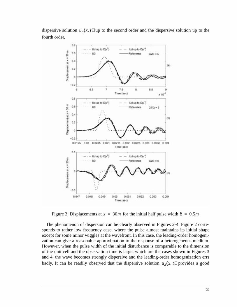
Evolution of displacements of the point ( m) is plotted in figures 2-4 for three

cases corresponding to m, m and m, respectively. In other

words, the ratios between the pulse width and the unit cell dimension are 8, 5 and3, respectively. Each of the figures 2-4 depicts four graphs corresponding to the finite ele-ment solution of the source problem, the analytical nondispersive solution , the

r 7.30=

x0 20= f0 1.0=

x 30m= δ 0.8m=

x 30=

δ 0.8= δ 0.5= δ 0.3=

2δ Ω⁄

u0 x t,( )

20

dispersive solution up to the second order and the dispersive solution up to the

fourth order.

Figure 3: Displacements at for the initial half pulse width

The phenomenon of dispersion can be clearly observed in Figures 2-4. Figure 2 corre-sponds to rather low frequency case, where the pulse almost maintains its initial shapeexcept for some minor wiggles at the wavefront. In this case, the leading-order homogeni-zation can give a reasonable approximation to the response of a heterogeneous medium.However, when the pulse width of the initial disturbance is comparable to the dimensionof the unit cell and the observation time is large, which are the cases shown in Figures 3and 4, the wave becomes strongly dispersive and the leading-order homogenization errsbadly. It can be readily observed that the dispersive solution provides a good

ud x t,( )

x 30m= δ 0.5m=

ud x t,( )

21

approximation to the response of the heterogeneous media even as the initial pulse widthis only 3 times of the unit cell dimension.

Figure 4: Displacements at for the initial half pulse width

6. Concluding Remarks Mathematical homogenization theory with multiple spatial and temporal scales havebeen investigated. This work is motivated by our recent studies [11][12] which suggestedthat in absence of multiple time scaling, higher order mathematical homogenizationmethod gives rise to secular terms which grow unbounded with time. In attempt todevelop a uniformly valid dispersive model up to an arbitrary order we extend the theorydeveloped in [12] to fast spatial scale and a series of slow temporal scales.

In our future work we will focus on the following two issues: (i) generalization to themultidimensional case, and (ii) a finite element implementation.

x 30m= δ 0.3m=

22

Acknowledgment This work was funded by Sandia National Laboratories. Sandia is a multi-programnational laboratory operated by the Sandia Corporation, a Lockheed Martin Company, forthe United States Department of Energy under Contract DE-AL04-94AL8500.

References 1 Sun, C.T., Achenbach, J.D., and Herrmann G., “Continuum theory for a laminated

medium”, ASME Journal of Applied Mechanics. Vol.35, 1968, pp. 467-475.2 Hegemier, G.A., and Nayfeh, A.H., “A continuum theory for wave propagation in

laminated composites. Case I: propagation normal to the laminates”, ASME Journal ofApplied Mechanics. Vol.40, 1973, pp. 503-510.

3 Bedford, A., Drumheller, D.S., and Sutherland, H.J., “On modeling the dynamics ofcomposite materials”, in: Mechanics Today, Vol. 3, Nemat-Nasser, S., ed., PergamonPress, New York, 1976, pp.1-54.

4 Sanchez-Palencia, E., “Non-homogeneous Media and Vibration Theory”, Springer,Berlin, 1980.

5 Benssousan, A., Lions, J.L. and Papanicoulau, G., “Asymptotic Analysis for PeriodicStructures”, North Holland, Amsterdam, 1978.

6 Bakhvalov, N.S., and Panasenko, G.P., “Homogenization: Averaging Processes inPeriodic Media”, Kluwer, Dordrecht, 1989.

7 Gambin, B., and Kroner, E., “High order terms in the homogenized stress-strain rela-tion of periodic elastic media”, Phys. Stat. Sol., Vol.51, 1989, pp. 513-519.

8 Boutin, C., “Microstructural effects in elastic composites”, Int. J. Solids Struct. 33(7),1996, pp.1023-1051.

9 Boutin, C., and Auriault, J.L, “Rayleigh scattering in elastic composite materials”, Int.J. Engng. Sci. 31(12), 1993, pp.1669-1689

10 Kevorkian, J., and Bosley, D.L., “Multiple-scale homogenization for weakly nonlin-ear conservation laws with rapid spatial fluctuations:, Studies in Applied Mathematics,Vol.101, 1998, pp.127-183.

11 Fish, J., and Chen, W., “High-order homogenization of initial/boundary-value prob-lem with oscillatory coefficients. Part I: One-dimensional case”, submitted to ASCEJournal of Engineering Mechanics, 1999.

12 Chen, W., and Fish, J., “A dispersive model for wave propagation in periodic hetero-geneous media based on homogenization with multiple spatial and temporal scales”,submitted to ASME Journal of Applied Mechanics, 2000.

13 Santosa, F., and Symes. W.W., “A dispersive effective medium for wave propagationin periodic composites”, SIAM J. Appl. Math., 51(4), 1991, pp. 984-1005.

14 Francfort, G.A., “Homogenization and linear thermoelasticity”, SIAM J. Math. Anal.,14(4), 1983, pp. 696-708.

15 Mei, C.C., Auriault J.L., and Ng, C.O., “Some applications of the homogenizationtheory”, in: Advances in Applied Mechanics, Vol. 32, Hutchinson, J.W., and Wu, T.Y.,eds., Academic Press, Boston, 1996, pp. 277-348.

16 Boutin, C., and Auriault, J.L., “Dynamic behavior of porous media saturated by a vis-coelastic fluid. Application to bituminous concretes”, Int. J. Engng. Sci., 28(11), 1990,pp.1157-1181.

Documents

Uniformly Valid Multiple Spatial-Temporal Scale …jfish/Unif_Valid.pdf1 Uniformly Valid Multiple Spatial-Temporal Scale Modeling for Wave Propagation in Heterogeneous Media Jacob