Uninformed Search (cont.)

Jim Little

UBC CS 322 – Search 3September 15, 2014

Textbook §3.0 – 3.4

1

Slide 2

Lecture Overview

• Recap DFS vs BFS

• Uninformed Iterative Deepening (IDS)

• Search with Costs

Slide 3

Search Strategies

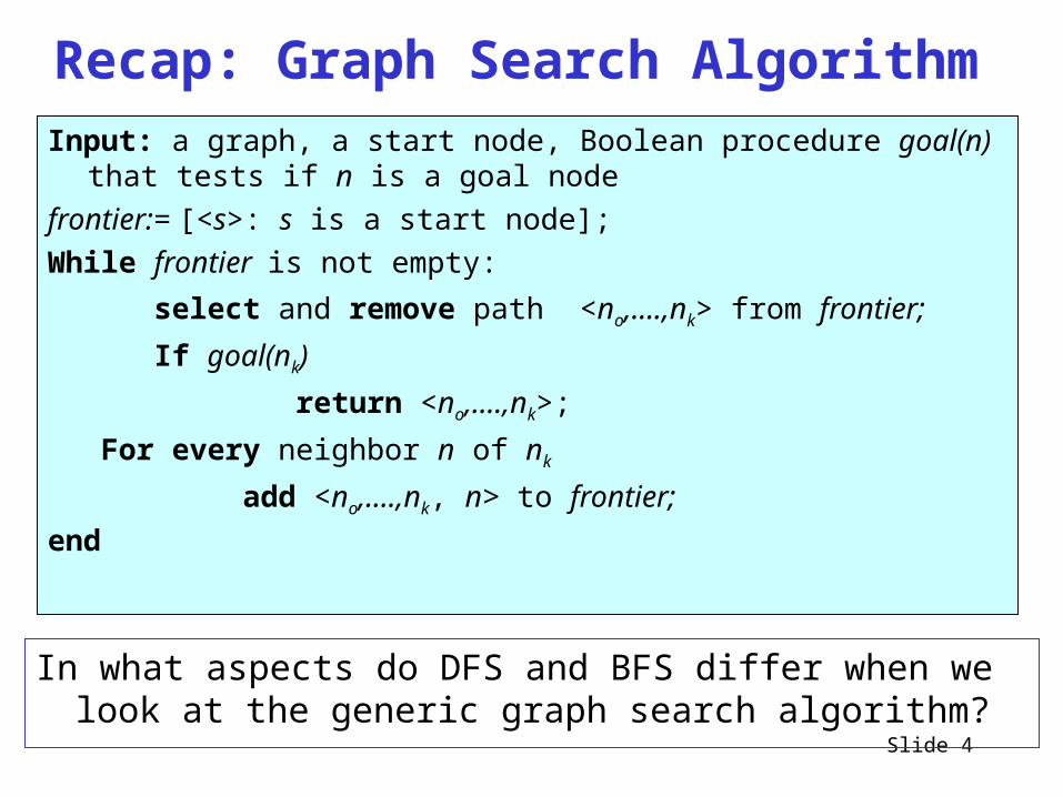
Recap: Graph Search Algorithm

Slide 4

Input: a graph, a start node, Boolean procedure goal(n) that tests if n is a goal node

frontier:= [<s>: s is a start node];

While frontier is not empty:

select and remove path <no,….,nk> from frontier;

If goal(nk)

return <no,….,nk>;

For every neighbor n of nk

add <no,….,nk, n> to frontier;

end

In what aspects do DFS and BFS differ when we look at the generic graph search algorithm?

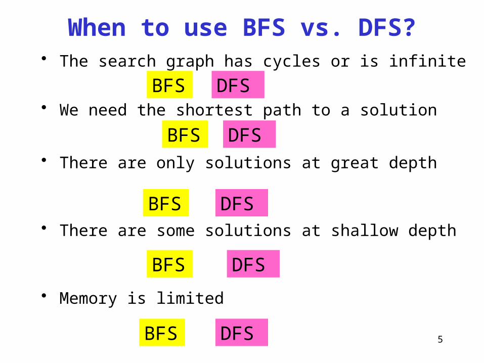
When to use BFS vs. DFS?

5

• The search graph has cycles or is infinite

• We need the shortest path to a solution

• There are only solutions at great depth

• There are some solutions at shallow depth

• Memory is limited

BFS DFS

BFS DFS

BFS DFS

BFS DFS

BFS DFS

Slide 6

Lecture Overview

• Recap DFS vs BFS

• Uninformed Iterative Deepening (IDS)

• Search with Costs

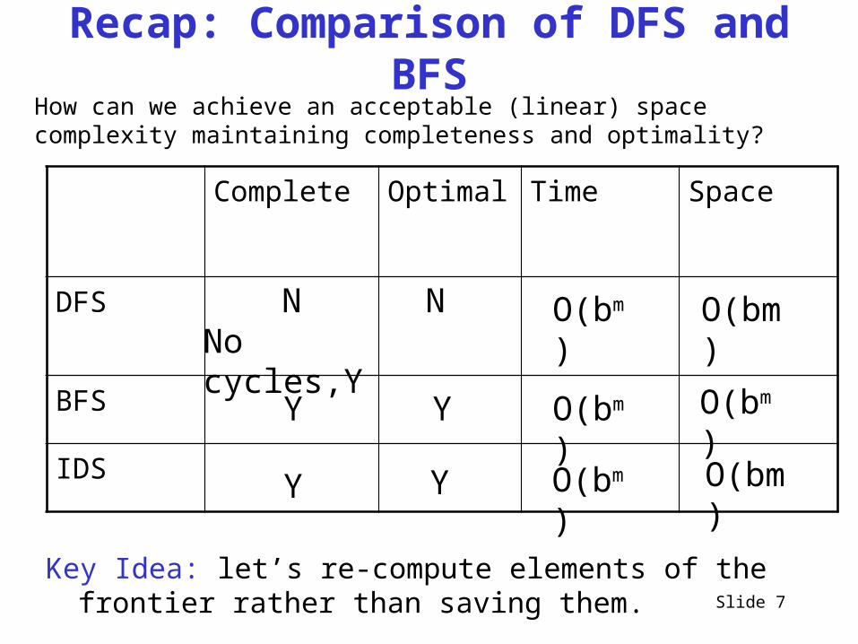
Recap: Comparison of DFS and BFS

Slide 7

Complete Optimal Time Space

DFS

BFS

IDS

O(bm) O(bm)

O(bm) O(bm)N NNo cycles,Y

Y Y

How can we achieve an acceptable (linear) space complexity maintaining completeness and optimality?

O(bm) O(bm)Y Y

Key Idea: let’s re-compute elements of the frontier rather than saving them.

Slide 8

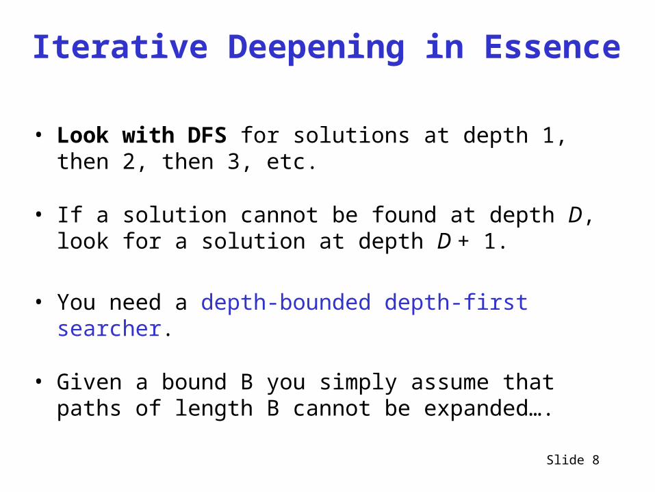
Iterative Deepening in Essence

• Look with DFS for solutions at depth 1, then 2, then 3, etc.

• If a solution cannot be found at depth D, look for a solution at depth D + 1.

• You need a depth-bounded depth-first searcher.

• Given a bound B you simply assume that paths of length B cannot be expanded….

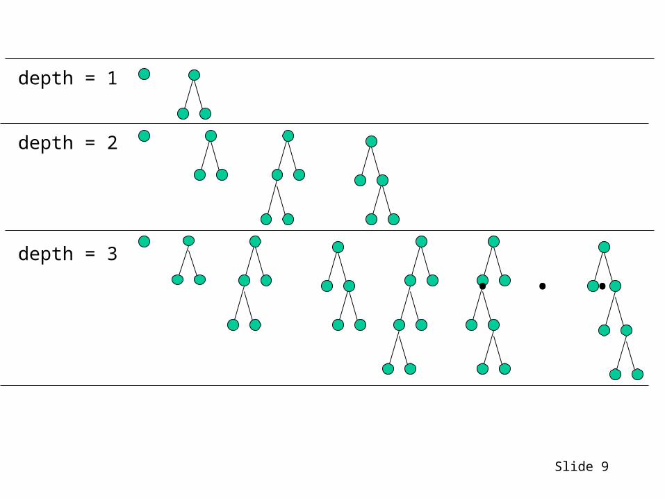
Slide 9

depth = 1

depth = 2

depth = 3

. . .

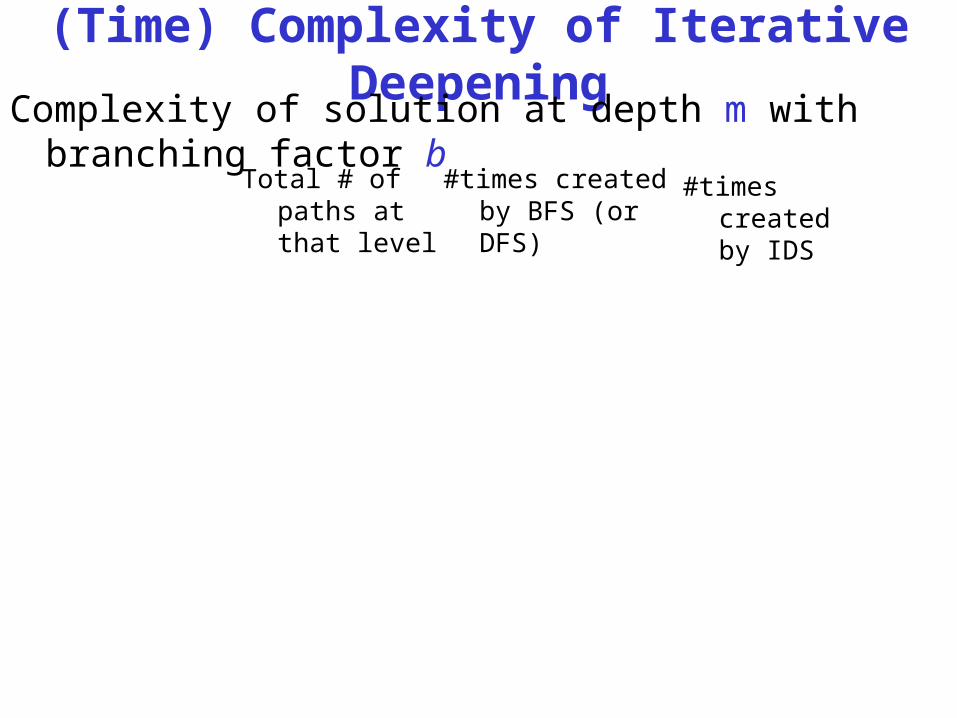
(Time) Complexity of Iterative Deepening

Complexity of solution at depth m with branching factor b

Total # of paths at that level

#times created by BFS (or DFS)

#times created by IDS

Slide 11

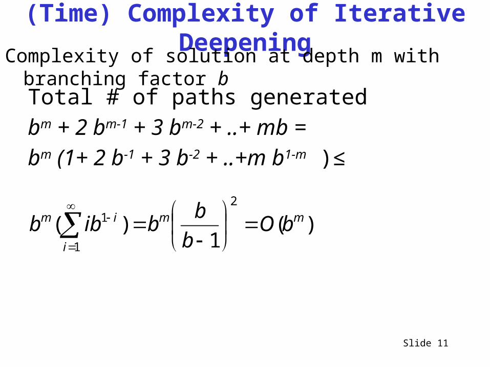
(Time) Complexity of Iterative Deepening

Complexity of solution at depth m with branching factor bTotal # of paths generatedbm + 2 bm-1 + 3 bm-2 + ..+ mb = bm (1+ 2 b-1 + 3 b-2 + ..+m b1-m )≤

)(1

)(2

1

1 mm

i

im bOb

bbibb

Slide 12

Lecture Overview

• Recap DFS vs BFS

• Uninformed Iterative Deepening (IDS)

• Search with Costs

Slide 13

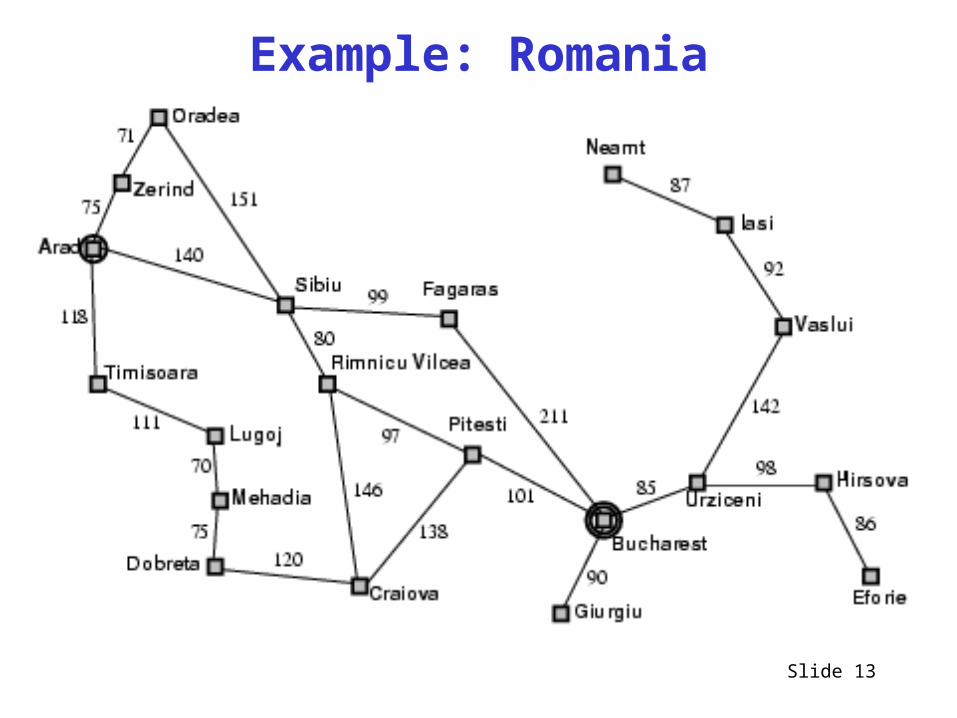
Example: Romania

Slide 14

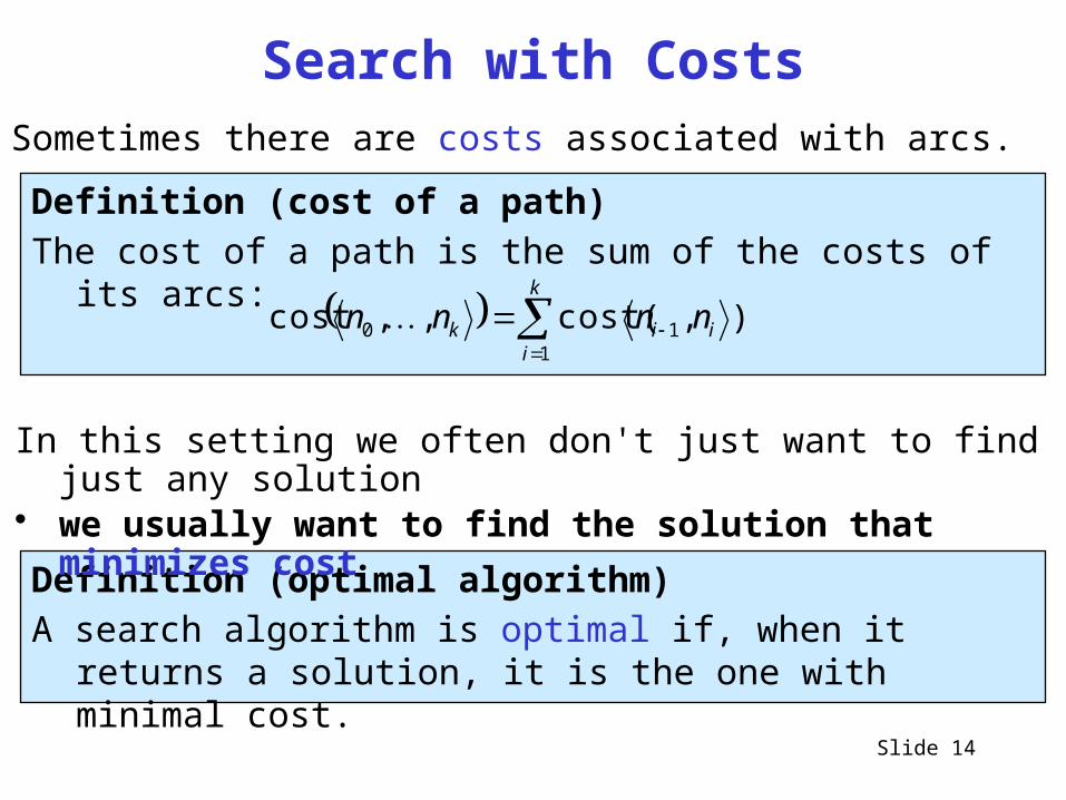
Search with CostsSometimes there are costs associated with arcs.

Definition (cost of a path)The cost of a path is the sum of the costs of its arcs:

Definition (optimal algorithm)A search algorithm is optimal if, when it returns a

solution, it is the one with minimal cost.

In this setting we often don't just want to find just any solution

• we usually want to find the solution that minimizes cost

),cost(,,cost1

10

k

iiik nnnn

Slide 15

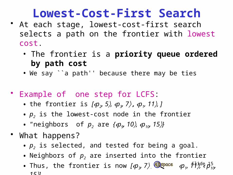
Lowest-Cost-First Search• At each stage, lowest-cost-first search selects a path

on the frontier with lowest cost.• The frontier is a priority queue ordered by

path cost• We say ``a path'' because there may be ties

• Example of one step for LCFS: • the frontier is [p2, 5, p3, 7 , p1, 11, ]

• p2 is the lowest-cost node in the frontier

• “neighbors” of p2 are {p9, 10, p10, 15}• What happens?• p2 is selected, and tested for being a goal.

• Neighbors of p2 are inserted into the frontier

• Thus, the frontier is now [p3, 7 , p9, 10, p1, 11, p10, 15].• ? ? is selected next.• Etc. etc.

Slide 17

Analysis of Lowest-Cost Search (1)

• Is LCFS complete?• not in general: a cycle with zero or negative arc

costs could be followed forever.• yes, as long as arc costs are strictly positive

• Is LCFS optimal?• Not in general. Why not?• Arc costs could be negative: a path that initially

looks high-cost could end up getting a ``refund''.• However, LCFS is optimal if arc costs are

guaranteed to be non-negative.

Slide 18

Analysis of Lowest-Cost Search

• What is the time complexity, if the maximum path length is m and the maximum branching factor is b?• The time complexity is O(bm): must examine

every node in the tree.• Knowing costs doesn't help here.

• What is the space complexity?• Space complexity is O(bm): we must store the

whole frontier in memory.

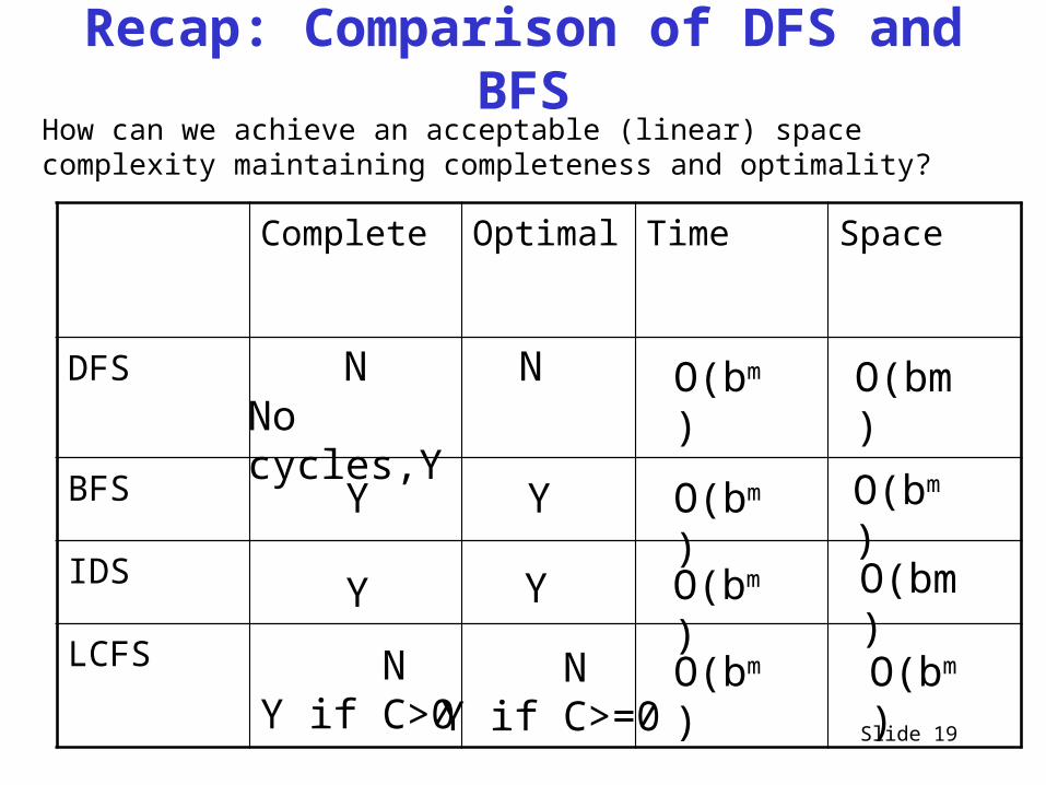
Recap: Comparison of DFS and BFS

Slide 19

Complete Optimal Time Space

DFS

BFS

IDS

LCFS

O(bm) O(bm)

O(bm) O(bm)N NNo cycles,Y

Y Y

How can we achieve an acceptable (linear) space complexity maintaining completeness and optimality?

O(bm) O(bm)Y Y

NY if C>0

NY if C>=0

O(bm) O(bm)

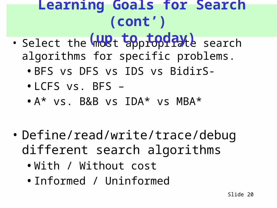
• Select the most appropriate search algorithms for specific problems. • BFS vs DFS vs IDS vs BidirS- • LCFS vs. BFS – • A* vs. B&B vs IDA* vs MBA*

• Define/read/write/trace/debug different search algorithms • With / Without cost• Informed / Uninformed

Slide 20

Learning Goals for Search (cont’) (up to today)

Slide 21

Beyond uninformed search….

Slide 22

Next Class

• Start Heuristic Search (textbook.: start 3.6)