Embed Size (px)
Citation preview
Program on Education Policy and Governance Working Papers Series
Union Reform and Teacher Turnover: Evidence from Wisconsin’s Act
Jonathan Roth1
PEPG 17-02
Harvard Kennedy School
79 JFK Street, Taubman 304 Cambridge, MA 02138
Tel: 617-495-7976 Fax: 617-496-4428 www.hks.harvard.edu/pepg/
1 Harvard University, [email protected].
Union Reform and Teacher Turnover: Evidence from Wisconsin’s Act
10
By Jonathan Roth∗
Draft: August 4, 2017
This paper studies teacher attrition in Wisconsin following Act 10, a policy
change which severely weakened teachers’ unions and capped wage growth for
teachers. I document a sharp increase in turnover after the Act was passed,
driven almost entirely by the exit of older teachers, who faced strong incen-
tives to retire before the end of pre-existing collective bargaining agreements.
I find that student academic performance increased in grades with teachers
who retired following the reform, and I obtain similar results when instru-
menting for retirement using the pre-existing age distribution of teachers.
Differences in value-added between retirees and their replacements can po-
tentially explain some, but not all, of the observed academic improvements.
∗ Harvard University, [email protected]. I would like to thank Chris Avery, Alex Bell, Olivia Chi, Moya Chin,Paulo Costa, Ash Craig, Oren Danieli, Peter Ganong, Colin Gray, Nathan Hendren, Ariella Kahn-Lang, Tzachi Raz, numerousparticipants at the Harvard Labor Economics Lunch, and especially Larry Katz and Marty West for valuable comments.This material is based upon work supported by the National Science Foundation Graduate Research Fellowship under GrantDGE1144152.
1
UNION REFORM AND TEACHER TURNOVER 2
I. Introduction
Since 2010, eight states have passed legislation that has weakened teachers’ unions by restricting
the scope of collective bargaining, establishing right-to-work laws, or both.1 The question of how
such changes affect teacher recruitment and retention is an important component of the broader
debate regarding the influence of teachers’ unions on education quality. Critics argue that these
policies reduce teacher compensation, thereby impairing the ability of school districts to recruit
and retain high-quality teachers (e.g. Murnane et al., 1991; Dolton and Marcenaro-Gutierrez, 2011;
Wisconsin Budget Project, 2017). Yet others contend that unions allow teachers to earn rents above
their outside options (Hoxby, 1996), in which case the labor supply effects of reductions in union
power or cuts to compensation may be small. Moreover, even if teachers are responsive to these
policy changes, the effects on education quality will depend on whether high-quality or low-quality
teachers are more elastic to the changes.
Until recently, however, there had been few sharp policy changes to curb union power or re-
duce teacher compensation. Thus, little empirical evidence exists on how teacher labor supply
responds to such changes, and if so what are the effects of the resulting teacher turnover on stu-
dent achievement. This paper addresses this gap in the literature by examining the labor supply
response of teachers to one of the most extreme reforms in this area, Wisconsin’s Act 10, a 2011 law
which severely weakened teachers’ unions, capped wage growth, and increased mandatory pension
contributions for teachers.
I show that teacher attrition did, in fact, increase sharply following the school year during
which Act 10 was passed, rising by 4.0 percentage points (58 percent) relative to the year before.
However, this increase was driven almost entirely by an increase in teacher retirements: turnover
for teachers over the minimum retirement age of 55 increased from 17 to 35 percent relative to
the previous year, compared with an increase from 4.7 to 5.4 percent for teachers below age 55.
Moreover, a comparison of attrition rates by age in 2010 versus 2011 reveals a sharp divergence
precisely at age 55, the minimum retirement age.
Act 10 created strong short-run incentives for eligible teachers to retire prior to the expira-
tion of their district’s pre-existing collective bargaining agreement (CBA). Teachers who did so
were guaranteed collectively-bargained supplementary retirement benefits, such as retiree heath-
care, whereas teachers who waited to retire faced the risk that these benefits, which under Act
10 could no longer be collectively bargained, would be reduced or eliminated by the district. On
its own the heterogenous labor supply response by older and younger teachers in 2011 could be
explained by these short-run incentives or by differing elasticities to permanent changes, but addi-
tional evidence points to the short-run incentives as the primary factor. The statewide retirement
rate in Wisconsin spiked in 2011, when collective bargaining agreements were set to expire in the
1Idaho, Iowa, and Tennessee passed legislation restricting (or eliminating) collective bargaining; West Virginia and Missouriestablished right-to-work laws, which prohibit unions from charging non-union members fees to cover the costs of collective-bargaining; and Wisconsin, Indiana, and Michigan did both.
UNION REFORM AND TEACHER TURNOVER 3
vast majority of districts, and returned towards its pre-reform level the following year. Additionally,
the Milwaukee Public School system, which had an usually long pre-existing CBA, experienced a
spike in retirements in the final year of its pre-existing CBA, a pattern which was not seen in other
districts whose CBAs had expired earlier.
The more permanent components of Act 10 appear to have had a more modest effect on teacher
attrition. A simple calculation that takes the one-year percentage change in attrition for teachers
under age 55, who were not influenced by the short-term retirement incentives, and divides by the
one-year percentage change in average compensation, implies a separation elasticity of around 2.
Similarly-constructed estimates using the changes in attrition for older teachers after all pre-existing
CBAs had expired also produce estimates around 2. A handful of omitted factors likely bias these
calculations upwards. The longer-term labor supply response is thus consistent with Ransom and
Sims (2010), who estimate a district-level elasticity of 1.8, and lends some additional credibility to
Rothstein (2015)’s simulations that assume occupation-wide separation elasticities are below 2.2
I then turn to investigating the effects of the wave of retirements in 2011 on education quality in
Wisconsin. One might have expected the increase in retirements to have had a negative impact on
education quality. Retirees are typically replaced by less experienced teachers, many of whom are
novices, and a large literature suggests that there are returns to experience in teaching, particularly
early in the career (e.g. Papay and Kraft, 2015; Wiswall, 2013; Chetty, Friedman and Rockoff, 2014).
Additionally, turnover itself may be harmful for students, even holding teacher quality constant
(Ronfeldt, Loeb and Wyckoff, 2013; Akhtari, Moreira and Trucco, 2017). On the other hand, it
is possible that lower quality teachers are more responsive to incentives to retire (Fitzpatrick and
Lovenheim, 2014), in which case the wave of retirements could have been beneficial. The increase
in retirements could have benefited schools in other ways, as well. For instance, since older, more
experienced teachers are generally paid more, retirements may have freed up resources in school
budgets that could be spent more productively elsewhere.
I investigate the effects of the surge of retirements in 2011 on education quality using measures
of value-added (VA) in math and reading at the school-by-grade level. I first show that school-grade-
levels with a larger fraction of retirees in 2011 improved significantly in math VA in 2012, despite
having similar trends to other grades prior to the reform. If the changes in school-grade-level VA
were attributable entirely to the difference in value-added between retirees and their replacements,
then my estimates would imply that retirees raised their students math test scores by 0.09 standard
deviations (σ) less than their replacements. My point estimates also suggest that retirements are
associated with improvements in reading VA, although the magnitudes are somewhat smaller (0.05σ
versus 0.09σ) and not statistically significant across all specifications.
Of course, the OLS results will only identify the causal effect of retirements on VA if the fraction
of retirements in 2011 is uncorrelated with other changes occurring at the school-grade level. The
OLS estimates will be biased upwards if teachers retire in anticipation of negative shocks to student
2In various simulations, Rothstein (2015) uses elasticities varying from 0.5 to 1.5.
UNION REFORM AND TEACHER TURNOVER 4
performance (e.g. departure of an effective principal), and will be biased downwards if new policies
that improve education quality (e.g. the introduction of a new curriculum) also induce teachers
to retire. To address the possible endogeneity of retirements, I employ an instrumental variables
strategy in which I instrument for the fraction of retirees in 2011 using the fraction of teachers
over the minimum retirement age of 55 in 2011. This approach, which is similar to that used
by Fitzpatrick and Lovenheim (2014) to evaluate an Early Retirement Incentive (ERI) program
in Illinois, will overcome the endogeneity issues discussed above if school-grade-levels with higher
fractions of retirement-eligible teachers were no more likely to experience administrative changes or
other shocks that influenced education quality. Using this IV approach, I once again find positive
and significant effects of retirements on math VA, with point estimates slightly larger (although
not significantly different) than those obtained using OLS. My point estimates in reading are also
similar to those obtained using OLS, but the estimates are less precise and therefore not statistically
significant.
The similar pattern across the OLS and IV specifications increases our confidence that the
results for the impact of retirements on education quality are not confounded by other sudden
shocks to student performance. I provide additional evidence in favor of a causal interpretation by
showing that the results are robust to controls for principal turnover and changes in district funding,
and via a placebo test involving teachers just below the minimum retirement age. Although some
concerns remain related to confounding changes in policy at the school level, at minimum the results
indicate that the wave of retirements in 2011 was not as detrimental to student achievement as
the literature on teacher experience and turnover would suggest – either these retirements directly
improved student performance, or schools were able to fully compensate for the retirements via
other policies.
Finally, I assess what causal mechanisms might have contributed to the observed increases
in education quality following teacher retirements in 2011. Fitzpatrick and Lovenheim (2014)
suggest that teachers who respond to financial incentives to retire may have low value-added on
average. My results are consistent with differences in teacher value-added between retirees and
their replacements having played an important role, but I present evidence that suggests that other
mechanisms were at play as well. In particular, I find a strong association between retirements in
one grade-level and improvements in performance in other grade-levels in the same school. This
association cannot easily be explained by teacher switching, since it persists across grades that have
relatively few switchers between them (e.g. first to fourth grade). A possible explanation for this
result is that since older teachers are generally paid more, retirements may free up resources that
can be used to improve achievement school-wide. A back-of-the-envelope calculation using results
from the Project STAR experiment (Krueger, 1999) suggests that if these savings were spent on
something as effective as class size reduction, then this channel could account for over half of the
observed increases in performance. Teacher peer effects could also have played a role (Jackson and
Bruegmann, 2009).
UNION REFORM AND TEACHER TURNOVER 5
This paper relates to the literature on how teachers’ retirement decisions respond to financial
incentives. While previous work has generally focused on how retirement decisions respond to dis-
continuities in the benefit formula embedded in existing pension systems (Costrell and Podgursky,
2009; Costrell and McGee, 2010), or to policy changes that increase the generosity of retiree bene-
fits at various ages (Furgeson, Strauss and Vogt, 2006; Brown and Laschever, 2012; Brown, 2013;
Fitzpatrick and Lovenheim, 2014; Fitzpatrick, 2014; Koedel and Xiang, 2017), I examine how re-
tirement decisions respond to the impending loss of supplementary retiree benefits. Fitzpatrick and
Lovenheim (2014) also examine the impacts of retirements induced by benefit changes on student
achievement, and find similar improvements in the grade-levels previously taught by retirees. How-
ever, my paper sheds additional light on the mechanisms by which retirements may affect student
achievement. In particular, the presence of cross-grade spillovers suggests that the improvements
in student performance cannot be explained by differences in value-added alone, and indicates that
other mechanisms, such as the impact of retirements on school budgets or teacher peer effects, may
be important.
This paper also contributes to work evaluating the effects of recent legislation to curb the power
of teachers’ unions.3 Quinby (2017) examines the end of collective bargaining in Tennessee and
finds significant effects on compensation but not on test scores or teacher retention. Three other
recent papers examine Act 10 in particular. Litten (2016) studies the effects of Act 10 on teacher
compensation, but does not examine teacher turnover or student achievement. Baron (2017) finds
decreases in student performance in districts whose prior CBAs expired in 2011 relative to districts
with longer pre-existing CBAs, and proposes teacher retirements as a possible mechanism. He
documents a fall in average teacher experience in districts with shorter pre-existing contracts, but
does not directly measure teacher retirements or examine the incentives that induced them. The
most closely related paper is Biasi (2017), who also examines teachers’ labor supply responses to
Act 10. Her primary focus is on teacher transfers between districts, although she also documents an
increase in overall turnover rates and concludes that exiting teachers in 2011 were negatively selected
using a quality measure derived from test scores in the school-grade-levels taught by teachers prior
to the reform. My paper is distinctive in examining the differential incentives and labor-supply
responses of older and younger teachers following Act 10, as well as the first to directly study the
effects of retirements induced by the reform on subsequent student performance.
The paper is organized as follows. Section II provides additional context regarding Act 10.
Section III describes the data used in my analysis. In Section IV, I examine changes in teacher
turnover following Act 10. Section V presents the methodology and results regarding the relation-
ship between the increase in retirements and education quality. Section VI concludes.
3A related literature focuses on the rise of public sector collective bargaining, primarily in the 1960s and 70s (Hoxby, 1996;Lovenheim, 2009; Lovenheim and Willen, 2016). Recent papers have also examined how teacher turnover is affected by changesto tenure policies (Strunk, Barrett and Lincove, 2017) and pay-for-performance schemes (Fryer, 2013).

UNION REFORM AND TEACHER TURNOVER 6
II. Background on Act 10
A. The law’s contents and timing
Wisconsin’s Act 10 instituted five major changes that affected teachers’ unions or teacher
compensation directly.4 First, the Act restricted the scope of the collective bargaining process
to negotiation of base wages, thus excluding teacher benefits – including health care and pension
contributions by the district – from the collective bargaining process. Second, Act 10 prohibited
base wages for teachers to rise faster than the rate of price inflation (CPI-U), unless authorized
by a referendum. Third, the Act required that employees make a mandatory contribution to the
state-wide pension system, the Wisconsin Retirement System (WRS), which in 2011 amounted
to roughly 5.8 percent of salary. Prior to the reform, there nominally had been an “employee”
contribution, but this was paid by the district in the vast majority of cases – in 2010, employees in
the WRS actually contributed less than 0.7% of the so-called employee contributions. The WRS
benefit formula was left unchanged by the Act, however. Fourth, the Act instituted a number of
other measures that weakened teachers’ unions, including a prohibition on the collection of agency
fees,5 a restriction that collective bargaining agreements be no more than one year in length, and
a requirement that unions hold recertification elections every year. Fifth, the biennial budget
proposed concurrently with Act 10 reduced state general aid to public schools by 8.4 percent, and
cut revenue limits, which cap the total amount of combined revenue that school districts can receive
from state general aid and local property taxes, by 5.5 percent.6
All of the aforementioned changes, besides for the changes to education funding, came into
effect at the expiration of each district’s pre-existing collective bargaining agreement (CBA). In
the vast majority of districts, the pre-existing CBA expired in the summer of 2011, since the usual
practice was to negotiate two-year CBAs in lockstop with the state’s biennial budget. Only 16 of
the state’s 424 districts had pre-existing CBAs with later expiration dates (Litten, 2016).7 The
most notable of these was the Milwaukee Public Schools (MPS), which had a pre-existing contract
that expired at the end of June 2013. This contract arose after MPS and the union were unable
to come to an agreement in 2009, and then ultimately agreed to a contract in 2010 that lasted
through the end of the subsequent biennial budget.
4I focus here on the main impacts of the Act as it relates to teachers, although it should be noted that the Act applied toall public sector unions in Wisconsin (excluding police and fire). For more details about the Act, see the 2011 summary by theWisconsin Legislative Reference Bureau.
5Agency fees are mandatory charges to non-union members meant to cover the cost of collective bargaining. Laws banningsuch fees are often referred to as right-to-work laws.
6Federal aid and certain state categorical expenditures, such as aid targeted for students with special needs or for trans-portation, are not included in the revenue limits.
7Litten (2016) acquired the universe of union contracts from an anonymous organization. I was unfortunately unable toobtain access to comprehensive data on districts with extended CBAs and their timing. However, newspaper accounts suggestthat all pre-existing contracts expired by the summer of 2013 or earlier (e.g. Richards, 9/12/13).
UNION REFORM AND TEACHER TURNOVER 7
B. Effects on compensation
Figure 1 plots the time series of average real salary and fringe benefits for teachers in Wisconsin.
The value of fringe benefits is estimated by the district for each of its employees as part of annual
reports to the Department of Public Instruction (DPI), and incorporates employer contributions
to health insurance and the pension system, as well as other benefits such as life and disability
insurance. The change in teacher compensation around the introduction of Act 10 is notable.
After rising slowly in the pre-period, average real compensation fell by $5813 (7.2 percent) in 2012,
the first year after the reform, and continued to fall somewhat afterwards. The drop was driven
primarily by a fall in teacher benefits, which dropped by an average of $4944 (18.1 percent) in 2012.
This decrease in benefits is 9.2 percent of the pre-reform average salary, so the mandated pension
contributions discussed above can explain roughly half of the drop in fringe benefits. Changes
in healthcare benefits likely explain most of the remainder of the drop, as many districts either
switched over to cheaper health plans or increased the employee share of the premiums. Litten
(2016) investigates changes in teacher compensation following Act 10 in more detail, concluding
that the Act reduced compensation by roughly 8 percent.
C. Incentives for retirement-eligible teachers
In Section IV, I show that attrition increased markedly for teachers over the minimum re-
tirement age of 55 following the school year during which Act 10 was passed, with much smaller
changes for other teachers. The features of the Act that created incentives for teachers to retire
therefore deserve particular attention.
Prior to the Act, former teachers received two forms of retirement benefits – pension payments
from the centralized Wisconsin Retirement System (WRS), which were determined at the state
level, and supplementary retirement benefits provided by the district as part of the local collective
bargaining agreement. These supplementary benefits typically included retiree health insurance,
and in some cases included other benefits such as supplemental pensions and life insurance.8 As
mentioned in Section II.A, Act 10 required working teachers to contribute a fraction of salary to
the pension system, but it did not make any changes to the pension benefits for retirees.
Act 10 did, however, have a profound impact on the supplementary retirement benefits pro-
vided by school districts. Under the Act, the district was required to honor these benefits for
teachers who retired prior to the end of the pre-existing collective bargaining agreement, but de-
termination of these benefits was left solely at the discretion of the districts once their pre-existing
CBA had expired. Thus, teachers who retired before the end of their districts’ pre-existing CBA
were guaranteed their collectively-bargained retirement benefits, whereas teachers who waited past
this point faced the risk of these benefits being reduced or eliminated by the school district. An
anonymous survey of district administrators conducted by the Milwaukee Journal Sentinel suggests
8I thank David Umhoefer of the Milwaukee Journal Sentinel and Pat Deklotz, Superintendent for the Kettle Moraine SchoolDistrict, for helpful conversations about the range of benefits provided prior to the Act.
UNION REFORM AND TEACHER TURNOVER 8
that approximately two-thirds of districts reduced or eliminated their post-employment benefits
packages in the five years after the Act’s passage (Umhoefer and Hauer, 2016). Moreover, substan-
tial uncertainty existed in 2011 as to what districts would do, and the threat of losing benefits may
therefore have influenced teachers’ retirement decisions even in districts where benefits were not
ultimately reduced or where grandfathering clauses were established.
The case of the Milwaukee Public Schools (MPS), Wisconsin’s largest school district, provides
a useful illustration of the magnitude of the changes to supplementary retirement benefits. Under
the pre-existing CBA in Milwaukee, retiring teachers could remain on their district health plan
until they became eligible for Medicare at age 65, and the district would pay a subsidy equal to
that in place for employees at the time of their retirement.9 This benefit was available to teachers
age 55 and older with at least 15 years of experience at the time of their retirement. MPS made two
policy changes that greatly reduced the generosity of its retiree health benefits for teachers retiring
after the expiration of its pre-existing CBA. First, the district eliminated retiree health benefits
for teachers who were under the age of 60 or had fewer than 20 years of experience at the date of
their retirement.10 Second, the district required active employees to contribute a higher fraction
towards healthcare premiums. This led to a fall in the subsidies for retirees, which are based on
the district’s subsidy at the time of retirement. Table 1 shows the impact that these changes had
on the retiree health benefits received by a representative teacher in Milwaukee before and after
the expiration of the pre-existing CBA. The table underscores the strong incentives to retire before
the expiration of the pre-existing CBA: a representative teacher who was age 55 in the final year of
the pre-existing CBA would lose over $18k in annual health benefits for each of the next 10 years
if she chose to postpone retirement by one year.
III. Data
A. Staffing Data
The Wisconsin Department of Public Instruction (DPI) annually publishes on its website an
individual-level dataset containing information on all staff members working in the Wisconsin public
school system as of the first week in September. I use these All Staff files for the 1995-6 through
2015-6 school years. The covariates include staff member first and last name, and basic demographic
information such as year of birth, gender, race, level of education, and local and total experience
in education. The year of birth information allows me to determine whether a teacher is above or
below the minimum retirement age of 55.11 The All Staff files also contain information on each
teacher’s base salary, an estimate of the value of the total value of the benefits that they receive
from the district, as well as a description of the teacher’s position in the school and the range of
9At age 65, retirees were required to enroll in Medicare, and the district would pay for supplementary insurance benefits.10A two-year grandfathering period was established for teachers age 55 and older with 30 or more years of experience. By
my calculations, less than 10% of teachers aged 55-59 had the requisite experience to qualify.11I calculate a teacher’s age at the end of a particular school year as the calendar year minus the teacher’s year of birth.
Since I do not see month of birth, some teachers born in the latter part of the year will be characterized as retirement-eligiblewhen they were only 54 at the end of the relevant school.
UNION REFORM AND TEACHER TURNOVER 9
grades they serve (e.g. Regular Education - English - Grades 6 to 8). In my primary analysis, I
restrict the sample to staff members categorized as regular education teachers.
I use the All Staff files to determine whether each teacher was retained from one year to the
next. I say that a teacher was retained between year t and year t + 1 if they worked as a regular
education teacher anywhere in the Wisconsin public school system in both years; otherwise I say
that the teacher attrited.12 Note that under this definition, a person who works as a teacher in one
year and transitions to an administrative role the next will be classified as having exited teaching.
This approach concords with the definition of turnover used by the National Center for Education
Statistics (Goldring, Taie and Riddles, 2014).
For the 2008-09 school year onwards, the All Staff files contain individual-level teacher identifiers
that are constant across years, allowing me to accurately measure whether a teacher was retained
for those years. There is no common identifier across years for the files prior to 2008-09, and so
I match individuals across years on first name, last name, and year of birth.13 Appendix Figure
A5 shows the imputed and true turnover rates for the years that unique identifiers are available.
Turnover rates follow very similar patterns using both methods, although attrition is somewhat
higher using the matching method; the primary reason for this appears to be that teachers’ last
names may change if they get married, which explains why the gap is smaller for retirement-eligible
teachers and for men, who are less likely to get married and change their names. In figures that
show the time series of turnover rates for a particular group of teachers, I adjust the turnover rates
for years before 2009 by the average measurement error for the relevant population between 2009
and 2014.14 For instance, between 2009 and 2014, the matching procedure produced a turnover
rate for teachers under the age of 55 that was on average 1.9 percentage points higher than the
true turnover rate. Thus, when I plot aggregate turnover rates for teachers below 55 (Figure 3),
I subtract 1.9 percentage points from the turnover rate for teachers under 55 calculated using the
matching procedure for years prior to 2009.
I also use the individual-level staffing data to compute turnover rates and other aggregates (e.g.
the fraction over age 55) at the school-by-grade level, since my measures of student performance
are at the school-by-grade level. When computing aggregates at the school-by-grade level, I weight
teachers by the number of full-time equivalent (FTE) units of their assignment (i.e., a full-time
teacher gets weight 1, a half-time teacher gets weight 0.5). I focus my analysis of turnover and
student performance on elementary school teachers in third through fifth grade, since over 85
percent of such teachers teach only one grade, and it is therefore relatively straightforward to
match teachers to the school-grade-level which they teach. In the instances where a teacher teaches
multiple grades, I do not see how their time is split between grades, and I therefore assume that
12I will use the terms teacher “turnover” and “attrition” interchangeably to mean the opposite of teacher retention.13There are a small number of first name, last name, year of birth combinations that appear multiple times in the same
year (e.g. Alison Johnson, born 1953). I drop all observations for such combinations, since I am unable to determine whichobservations to match across years. Roughly 0.6% of observations are dropped because of this.
14In 2015, DPI switched to a new data management system, which standardized names between 2015 and 2016, effectivelyeliminating measurement error. I therefore do not include the measurement error for 2015 in computing the adjustment.
UNION REFORM AND TEACHER TURNOVER 10
their FTE units are split evenly across the grades that they teach; a full-time teacher teaching both
3rd and 4th grade will thus be counted as half a teacher in each of those grades.
B. School-Grade-Level Value-Added Data
I evaluate the impact of retirements on education quality using two measures of value-added in
reading and mathematics at the school-grade-year level. Both measures of value-added are based
on student performance on the Wisconsin Knowledge and Concepts Examination (WKCE), a state-
wide examination in math and reading administered to students in the Fall of the 2005-06 through
2013-14 school years.15 Again, I focus on value-added for elementary school (3rd through 5th grade),
since elementary school teachers typically teach only one grade, making it more straightforward to
link teachers to the grade-level that they taught.
Constructing value-added from WKCE scores. I construct the primary measure of value-
added used in my analysis using publicly available data on the mean WKCE score at the school-
grade-year level. Intuitively, my school-grade-level value-added metric is based on the growth in
scores for a cohort of students within a school. For instance, the value-added metric for third grade
in Hamilton Elementary school in the 2010-11 school year is derived based on how well students at
Hamilton scored on the test administered at the beginning of fourth grade in 2011, relative to what
we would have expected given the scores for the same cohort of students on the test administered
at the beginning of third grade in 2010. Formally, I normalize the school-grade-year mean scores
by the mean and standard deviation of the state-wide distribution for students in each grade, so
that the units of school-grade-year means are z-scores of the student distribution for each grade. I
then predict (normalized) math test scores using the following regression:
Y maths,g+1,t+1 = β0 + Y math
s,g,t β1 + Y readings,g,t β2 +Xs,g,t β3 + εs,g,t
where Y maths,g,t and Y reading
s,g,t are the normalized mean test scores for students in math and reading
for grade g in school s in year t. Xs,g,t is a vector of covariates describing the demographics of the
students in grade g in school s in year t – namely, the fraction of students who are (non-hispanic)
black, hispanic, receive free or reduced price lunch, are characterized as English language learners,
and are characterized has having disabilities. I attribute the difference between the predicted score
and the actual score, i.e. εs,g,t, as the math value-added of grade g in school s in year t. I follow
an analogous procedure for reading.
During the time period studied, the WKCE examination was administered in October, close
to the beginning of the school year, and so I construct the value-added for the fourth grade, for
instance, using the growth in test scores between the beginning of 4th grade and the beginning of
5th grade the following year (and likewise for other grades). This is consistent with the practice used
15After conducting the WKCE examination in the Fall from 2005 to 2013, Wisconsin switched to a spring test administrationin 2015, effectively going 2 school years between tests. Additionally, they implemented a new test, called the Badger Examin 2015, before switching to a third test, the Wisconsin Forward Exam, in 2016. It is thus difficult to construct a consistentvalue-added series past 2013.
UNION REFORM AND TEACHER TURNOVER 11
by DPI in constructing its internal value-added estimates. Since my value-added metric requires
me to match scores for cohorts in adjacent grades, I am unable to construct a value-added measure
for a particular school-grade unit if it is the highest grade offered in the school. This is generally
not an issue for third and fourth grade, but leads to missing value-added for the majority of fifth
grades, since elementary schools often end in fifth grade (see Appendix Table A2). I obtain very
similar results when excluding fifth grade classrooms from the analysis.
VARC Value-Added. In addition to the school-grade-level value-added metric constructed
above, I also obtained access to a school-grade-level value-added metric constructed by the Wiscon-
sin Value-Added Research Center (VARC) for internal evaluation by DPI. The primary advantage
of the VARC value-added measure is that it covers nearly the universe of third through fifth grades
(Appendix Table A2). This is because the VARC value-added measure is based on a student-level
dataset (which I do not have access to), which allows them to track students across years even
if they change schools. The student microdata also allows them to include student-level controls
which are not available to me.
Unfortunately, the VARC data also have a few shortcomings. First and foremost, the value-
added metrics provided by VARC have had a complex shrinkage procedure applied to them which
cannot be reversed given the information available to me. It is problematic to use shrunk measures
of value-added as an outcome variable since they will typically change less than one-for-one with
changes in true effectiveness, and thus we would expect the results to be attenuated towards zero (see
Schwartz, 2015 for a discussion). In addition, the control variables used by VARC vary somewhat
across years, and for some years VARC reports a value-added metric in the unit of student test
scores, whereas in other years they report only a z-score of the school-grade-level value-added.
As a result, I focus on the school-grade-level value-added discussed above in my main analysis.
Nonetheless, in Appendix A.A1 I reproduce my primary analysis using a standardized version of
the VARC value-added measures. For the most part, the results follow quite similar patterns to
those with my main value-added measure – both when using the full VARC sample, as well as the
VARC value-added measure for the subsample for which I am able to construct my main analysis.
This gives some confidence that the main results are not driven by the exact specification or sample
for the value-added, and I note in the text the few places where the results appear to be sensitive
to these choices.
School-Grade-Level versus Individual-Teacher Value-Added. Wisconsin does not have
student-teacher linkages for the WKCE examination, and so it is not possible to construct indi-
vidual teacher-level value-added for the period studied. However, even if individual TVA were
available, school-grade-level value-added may be a more appropriate metric for measuring the im-
pacts of teacher retirements on education quality. First, there may be spillover effects across
teachers (Jackson and Bruegmann, 2009) or negative impacts of turnover per se (Ronfeldt, Loeb
and Wyckoff, 2013), which will be captured by changes in school-grade-level value-added but not
by the pure differences in TVA between retirees and their replacements. Along similar lines, as I
UNION REFORM AND TEACHER TURNOVER 12
discuss in Section V.E, it is also possible that retirements affect education quality by freeing up
resources, which again will not be captured by differences in individual TVA. Moreover, concerns
about bias in individual TVA owing to endogenous sorting of students to teachers (Rothstein, 2009)
may be particularly strong following teacher retirements, as principals may assign particular types
of students to novice teachers. Grade-level value-added, which examines the growth of an entire
cohort of students, alleviates these concerns.
IV. Teacher Attrition Following Act 10
Figure 2 plots the time series of aggregate turnover rates for regular education teachers in Wis-
consin’s public schools. The figure shows a sharp increase in turnover (from 7.0 to 11.0 percentage
points) following the 2010-2011 school year – that is, following the school year during which Act 10
was passed.16 Aggregate turnover rates come back down after 2011, but remain above their 2010
levels from 2012 through 2015.
The increase in aggregate turnover rates in 2011 was driven almost entirely by teachers of
retirement-eligible age. This can be seen in Figure 3, which plots attrition separately for teachers
above and below the age of 55, which is the minimum age at which one is eligible to receive pension
benefits from the statewide Wisconsin Retirement System. The differences between the two groups
are striking: between 2010 and 2011, attrition increases from 17 to 35 percent for teachers of
retirement-eligible age, and from 4.7 to 5.4 percent for teachers below the retirement age. The
importance of retirement-eligibility for attrition in 2011 is further highlighted in Figure 4, which
plots attrition by age following the 2010 and 2011 school years. Attrition rates in 2010 and 2011
appear fairly similar at all ages under 55, and begin to diverge sharply precisely at the minimum
retirement age of 55.
On its own, the sharply heterogenous labor-supply response by retirement-eligibility could have
been the result of two different channels. First, as discussed in Section II.C, retirement-eligible
teachers faced strong incentives to retire before the expiration of their district’s pre-existing CBA
in order to guarantee that they received collectively-bargained supplementary retirement benefits.
Second, it is possible that teachers with the option of taking a generous retirement package are
more elastic to permanent changes to compensation and union status than are other teachers.
However, additional evidence suggests that the incentives to retire earlier to receive collectively-
bargained retirement benefits were the predominant factor behind the surge in retirements in 2011.
First, after rising to 35 percent in 2011, when the vast majority of districts’ pre-existing CBAs were
set to expire, attrition rates for teachers over 55 fell to 23 percent in 2012. By 2014, when all of the
pre-existing collective bargaining agreements had expired, retirement rates had fallen somewhat
further, to 21 percent, just 3.5 percentage points above their 2010 levels. One might worry that the
fall in retirement rates after the initial spike in 2011 is the result of a selection effect in which only
16The turnover rate plotted for the year 2011 in Figure 2 represents the fraction of regular education teachers in the 2010-2011school year who did not teach the following year, i.e. those who appear to have left the system in the summer of 2011. I willhenceforth refer to school years by the calendar year in which they end (e.g. 2010-2011 as 2011).
UNION REFORM AND TEACHER TURNOVER 13
the most attached older teachers remained in the system. However, since the changes in attrition
for teachers under the age of 55 were relatively small, we would not expect much of a selection
effect for teachers age 55, i.e. those who are newly eligible to retire. Appendix Figure A6 shows
that retirement rates for newly-eligible teachers follow similar patterns to those for all retirees,
indicating that the drop in retirement rates in 2012 is likely not explained by selection.
Further evidence on the importance of the short-run incentives comes from a comparison of
turnover rates for older teachers in the Milwaukee Public Schools (MPS) versus the rest of Wis-
consin. As mentioned in Section II.A, MPS had an unusually long pre-existing CBA that expired
in 2013, whereas the vast majority of districts had contracts expiring in 2011. Figure 5 shows that
MPS experienced a large spike in retirements in 2013, when its pre-existing CBA was set to expire,
a pattern which was not seen in other districts whose CBAs had primarily expired earlier.17
Although the predominant factor in the rise in attrition following Act 10 appears to have been
the short-run incentives for teachers to retire, the evidence is consistent with the more permanent
components of the Act having had a modest effect on teacher attrition. After experiencing declines
every year since 2003, attrition for teachers under the age of 55 rose 0.7 percentage points (16
percent) in 2011 and continued to rise over the next 3 years (Figure 3). Additionally, as discussed
above, retirement rates remained about 3 percentage points above their pre-reform levels even
once all pre-existing CBAs had expired. A naive calculation that takes the percent change in
turnover for teachers under the age of 55 between 2011 and 2010 and divides by the percent change
in average total real compensation for these teachers in the first year after the reform yields a
separation elasticity of 2.2. Similarly, if we take the percent change in turnover for older teachers
between 2010 and 2014, once all pre-existing CBAs had expired, and divide by the percent change in
compensation for older teachers, we obtain a naive separation elasticity estimate of 1.7. Appendix
Table A1 shows these calculations for other years as well.
One ought to be cautious in interpreting these naive elasticities as the causal impact of Act
10, since other concurrent changes in Wisconsin could also have had modest effects on teacher
turnover rates. For instance, Wisconsin’s economy was generally improving in the period following
Act 10’s introduction, and the state implemented a new teacher evaluation program in the 2014-
2015 school year.18 Additionally, in the absence of any confounding factors, we would generally
expect these naive estimates to exceed the elasticity of separation with respect to a permanent
change in compensation, since Act 10 appears to have reduced not just the level of compensation
but also its growth rate. All of these omitted factors likely bias the naive elasticity estimates
upwards, and so it seems reasonable to view these as an upper bound on the elasticity of separation
17Figure 5 shows that Milwaukee also experienced a spike in retirements in 2011, following the school year during which Act10 was announced. Two factors may have contributed to this spike: first, some forward-looking teachers may have responded tothe announcement of Act 10, even if it did not come into effect immediately in their district. Second, as part of the pre-existingCBA in Milwaukee, beginning in the 2011-2012 school year teachers were required to contribute 1-2% of their salary towardstheir health insurance. Since retiree healthcare benefits depend on the district contribution at the time of retirement, teacherswho retired in 2011 received more generous retiree healthcare benefits than those who retired later.
18DPI also ran smaller pilots of the evaluation program in 2012-3 and 2013-4, covering roughly 600 and 1200 teachersrespectively (out of over 50,000 total teachers in the state).
UNION REFORM AND TEACHER TURNOVER 14
with respect to permanent changes in compensation at the state level. As a point of comparison,
Ransom and Sims (2010) estimate that the elasticity of separation with respect to changes in
compensation at the district level is 1.8. The naive estimates are thus of a fairly similar magnitude,
suggesting that the observed rise in attrition for younger teachers, and the longer-run rises in
attrition among retirement-eligible teachers, might plausibly have resulted from Act 10’s impact
on teacher compensation.
In sum, the short-run incentives to retire created by Act 10 appear to have caused a large spike
in retirements, with attrition doubling from 17 to 35 percent for teachers of retirement-eligible age
in the first year after the reform. Identifying the longer-run effects of the Act is more difficult,
although the results are consistent with Act 10 having contributed to a more modest rise in the
longer-run turnover rates for both younger and older teachers, with effects plausibly as large as 2
or 3 percentage points.
V. The Effects of Teacher Retirements on Education Inputs and Quality
In this Section, I examine how the large increase in teacher retirements in 2011 affected the
composition of teachers and the quality of education in the grade-levels (and schools) that these
retirees left behind.
A. Empirical Strategy
I first describe the main empirical strategy and required assumptions for estimating the impacts
of teacher retirements in 2011 on subsequent outcomes. For clarity, I focus the discussion on the
strategy and required assumptions for the effects of retirements on value-added, which will be the
primary subject of this section, although I use an analogous methodology with parallel required
assumptions to analyze the effects of retirements on other outcomes such as teacher experience,
compensation, and student-teacher ratios.
I begin with an “event study” approach in which I compare the performance over time of
school-grade-levels with higher and lower fraction of retirees in 2011. Formally, I estimate OLS
regressions of the form:
ygst =∑
τ 6=2011
(frac retire2011)gs 1 [t = τ ] β1,τ+
∑τ
1 [t = τ ] β0,τ + φgs + εgst(1)
where ygst is value-added (or another outcome of interest) in grade g in school s at time t;
frac retire2011 is the fraction of teachers in the school-grade-level that retired in 2011; and φgs is
a school-grade-level fixed effect, which absorbs time invariant differences across school-grade-levels
with higher and lower fractions of retirees in 2011.
UNION REFORM AND TEACHER TURNOVER 15
The main coefficient of interest is β1,2012, which indicates how value-added changed between
2011 and 2012 in grades with higher fractions of retirees in 2011 relative to other grades. β1,2012
will identify the causal impact of retirements in 2011 on performance in 2012 under the assumption
that, absent any retirements in 2011, school-grade-levels with higher and lower fractions of retirees
would have had parallel trends.
I find that prior to 2011, school-grade-levels with higher and lower fractions of retirees had
similar trends in effectiveness – i.e. the β1,τ coefficients are generally close to 0 and insignificant.
Nonetheless, there is reason to be concerned that β1,2012 may not capture the causal impact of having
higher fractions of retirees in 2011 on school-grade-level performance, although the direction of the
bias is not obvious. If teachers choose to retire in anticipation of a negative shock to their school’s
performance – for instance, the retirement of a talented principal or disruptive construction outside
of the school building – then β1,2012 will be biased downwards. On the other hand, it is possible
that retirements in 2011 were correlated with policies that improved student achievement, in which
case the β1,2012 will be biased upwards. For instance, following the passage of Act 10 certain
principals may have attempted to exert more effort from their teachers or to impose a standardized
curriculum, simultaneously improving value-added and inducing a larger number of teachers to
retire. These endogeneity concerns would arise in any year, but they may be particularly sharp for
retirements following 2011, since the introduction of Act 10 may have given school administrations
more latitude to introduce new policies.
To address the potential endogeneity of retirements in 2011, I employ an instrumental vari-
ables strategy in which I instrument for the fraction of teachers retiring in 2011 with the fraction
of teachers over the minimum retirement age of 55 in 2011.19 This strategy will overcome the
endogeneity issues discussed above under the assumption that school-grade-levels with higher frac-
tions of retirement-eligible teachers are no more likely to experience policy changes or other shocks
that influence effectiveness. Although this assumption is plausible, there still may be some concern
that older teacher sorts to different types of schools (or grade-levels within a school), which may
react differently to the introduction of a reform like Act 10. I employ two strategies to address
this concern. First, I add controls for observable time-varying characteristics – such as principal
turnover and district-level funding – to see whether these affect the results. Second, I conduct a
falsification test in which I include the fraction of teachers just below the retirement-eligible age
(age 45 to 54) in addition to the fraction 55 and over. If the age distribution affects trends in
performance through the channel of retirements, then we would not expect to see sharp changes in
VA for school-grade-levels with higher fractions of teachers just below the minimum retirement age.
Conversely, if other factors that are correlated with age are driving the results, we would expect to
see similar patterns for near-retirement and retirement-eligible teachers.
19More precisely, since I observe birth-year but not birthdate, I use the fraction of teachers born in 1956 or earlier as theinstrument. A small number of teachers born in the latter part of 1956 will therefore be characterized as having been retirement-eligible in 2011 despite not having reached the minimum retirement age by the summer of 2011, when retirement decisions weremade.
UNION REFORM AND TEACHER TURNOVER 16
B. Results for Teacher Composition
Before proceeding to the main results using value-added, I first present evidence on how the
composition of teachers in a school-grade-level changed following the retirement of a teacher in 2011
(Figure 6 and Table 2). Perhaps unsurprisingly, school-grade-levels with higher fractions of retirees
in 2011 experience a drop in average teacher experience and compensation in 2012, and a rise in
the fraction of novice teachers, relative to other school-grade-levels. They also experience a small
rise in student-teacher ratios, as would occur if not all retirees are replaced, although the changes
are relatively small and statistically insignificant. Table 2 shows that the OLS and IV methods
produce fairly similar results for these outcomes.
C. Event-Study Results for School-Grade-Level Value-Added
The top panel of Figure 7 shows the OLS event study results for math value-added. The figure
shows that school-grade-levels with higher fractions of retirees in 2011 seemed to have fairly stable
value-added prior to the policy change – with, if anything, perhaps a slightly negative trend –
before improving significantly in the year following the policy change. The bottom panel of Figure
7 shows the analogous results using the instrumental variables strategy. The patterns are similar
to the OLS results, and the coefficient for 2012 is in fact even larger than using OLS. Similarly,
Figure 8 shows the OLS and IV results for reading VA. The results are qualitatively similar to
those for math, although the magnitude of the effects is smaller, and the IV estimate for 2012
is not significant (although it is similar in magnitude to the OLS coefficient).20 The similarity
between the IV and OLS results gives some confidence that the improvements in value-added in
grades with retirements are not driven by the endogeneity of retirements to school policies that
also improve performance.
To interpret the magnitudes of the coefficients, it is useful to consider the following simplified
model. Suppose that school-grade-level value-added is merely the average of the value-added of the
individual teachers in that school-grade-level, and that all of the changes in effectiveness between
school-grade-levels with and without retirees were driven by differences in effectiveness between
retirees and their replacements. Under these assumptions, β1,2012 would identify the average differ-
ence in value-added between retirees in 2011 and their replacements.21 Thus, the coefficient of 0.09
for math value-added would suggest that retirees raised their students’ test scores by 0.09 standard
deviations less than their replacements. Although these assumptions may not hold in practice –
teacher retirements may influence school-grade-level effectiveness through other mechanisms, for
20In Appendix A.A1, I reproduce analogous figures using school-grade-level value-added estimates constructed by VARC forinternal DPI review. The findings for math are quite similar to those presented here. In reading, the OLS results are againpositive but no longer significant, and the IV coefficient for reading flips sign, but again is insignificant. See the Appendix fora more detailed discussion.
21To see why this is the case, consider the case of a school-grade-level with 2 teachers in 2011, one of whom retired in2011 and was replaced by a teacher who raised student test scores by 0.1 standard deviations more than the retiree. If thesecond teacher remained and had the same effectiveness as before, then overall school-grade-level value-added would rise by0.05 standard deviations – precisely the fraction of teachers who retired (0.5) times the difference in value-added between theretiree and his replacement (0.1).

UNION REFORM AND TEACHER TURNOVER 17
instance – the model described above provides a useful framework for interpreting the magnitude
of the effects.
Table 4 summarizes the results when adding time-varying controls or time-varying fixed effects
to the main event-study specification. The coefficients are quite similar when adding controls for
district-level funding and for whether a school has a new principal, suggesting that district-level
changes in funding and principal turnover are not driving the observed increases in effectiveness in
school-grade-levels with more retirees. It is important to note, however, that the estimated effects
are smaller and not statistically significant (albeit less precise) when including school-by-year fixed
effects. The implication is that school-grade-levels with retirees in 2011 experience a sudden increase
in value-added in 2012, but so do nearby grades in the same school.22 This intuition is confirmed
in Figure 9, which shows estimates of equation (1) when collapsing the data to the school-by-year
level.
These patterns may contribute to concerns that the fraction of older teachers is correlated
with confounding schoolwide changes in 2012, although it is also possible that retirements have
causal spillover effects across school-grade-levels, as I discuss extensively in Section V.E. To try
to distinguish between the causal effects of retirements and unobserved confounding factors at the
school level that are correlated with the age distribution, I run placebo tests in which I regress the
growth in school-grade-level value-added between 2011 and 2012 on the fraction of teachers above
the retirement age (55-plus) and the fraction of teachers just below the retirement age (45 to 54).
The results are shown in Table 5. In math, the coefficient on the fraction age 55-plus is positive and
significant, whereas the coefficient on teachers 45 to 54 is smaller and not significant, as we would
expect if retirements, rather than other changes correlated with the age distribution, were driving
the results. However, I cannot rule out that the two coefficients are equal at conventional levels
(p-value = 0.17). Likewise, I do not find that either coefficient is significant for reading, which
is unsurprising given that the IV results were not significant for reading. Additionally, I show in
Appendix Table A3 that the coefficients for the placebo group are somewhat sensitive to the choice
of value-added and sample used. Thus, while the math results using the primary analysis sample
are suggestive in favor of a causal interpretation, I cannot fully rule out some role for omitted
variables correlated with the teacher age distribution.
D. Comparison to Previous Years and Implied Effects for Marginal Retirees
In Section V.C, I focused on the average effects of retirements in 2011 on subsequent education
quality. However, since some teachers would have retired regardless of the reform, we may be more
interested in the effects of the marginal retirement in 2011. Under certain additional assumptions,
we can estimate the average effect of a marginal retirement in 2011 by comparing the effects for
2011 shown above to similar estimates constructed in the pre-period. In particular, suppose that i)
22Recall that my analysis uses value-added for grades 3 to 5, so using school-by-year fixed effects compares, for instance, 3rdgrade in a school to 4th and 5th grades in the school in the same year.
UNION REFORM AND TEACHER TURNOVER 18
all teachers who would have retired in 2011 absent the reform retired anyway (monotonicity), and
ii) retirements of such always-takers had the same average effect on education quality as retirements
in the pre-period. It follows from these assumptions that the average effect of retirements in 2011
is just the weighted-average of the effects for marginal retirees and for retirees in the pre-period.
That is,
β2011 = αβmarginal2011 + (1 − α)βpre(2)
where α is the fraction of marginal retirees in 2011, and β2011, βmarginal2011 and βpre are respectively
the average effects of retirements for all teachers in 2011, for marginal teachers in 2011, and for
teachers in the pre-period. Equation (2) allows us to solve for the effect for marginal retirees in
terms of the average effects of retirements in 2011 and in the pre-period:
βmarginal2011 =1
αβ2011 −
1 − α
αβpre(3)
I jointly estimate β2011 and βpre by estimating the regression equation:
V At+1 − V At =frac retiret × 1 [pret]βpre + β0pre1 [pret] +(4)
frac retiret × 1 [2011t]β2011 + β020111 [2011t]
I estimate (4) both using OLS and by instrumenting for the fraction retired using the fraction
of teachers in the school-grade-level over age 55 (interacted with indicators for pre and 2011). The
parallel trends assumptions needed for identification are the same as those discussed in the previous
sections, except they must now hold for both 2011 and prior years. To calculate α, I assume that
absent Act 10 the retirement rate in 2011 would have been equal to that in 2010.
Table 6 shows the results for βpre and β2011 as well as the implied effects for marginal retirees in
2011. The point estimates indicate that in the pre-period, retirements were associated with modest
improvements in school-grade-level value-added, but the estimated effects are smaller than those
for 2011 and are significant only in the OLS specification for math. As a result, the estimated
effects for marginal retirees in 2011 are larger than the estimated average effects for 2011, although
they are also somewhat less precise. Nonetheless, the OLS and IV estimates of the marginal effects
are statistically significant in math, and the OLS results for reading allow us to rule out all but
very small negative marginal effects. The IV results for reading are too imprecise to draw strong
conclusions.
If the primary mechanism behind the changes in value-added was differences in teacher ef-
fectiveness between retirees and their replacements, then these results would suggest that the
UNION REFORM AND TEACHER TURNOVER 19
marginal retiree was particularly ineffective relative to the norm. This is consistent with Fitzpatrick
and Lovenheim (2014)’s suggestion that low value-added teachers may be the most responsive to
changes in teacher retirement incentives. The marginal effects estimates should be viewed with
some caution, however, because there are other plausible causal mechanisms that would lead to
violations of the assumptions needed to estimate the marginal effects. For instance, since retirees
generally earn less than their replacements, retirements may benefit education quality by freeing
up resources. Because the 2011 biennial budget reduced education funding, these effects may have
been larger in 2011 for all retirees, which would violate the assumption that “always-takers” had
the same effects as in previous years.
E. Possible Mechanisms
In this section, I consider what causal mechanisms might plausibly have driven the positive
effects of retirements in 2011 on subsequent value-added. One candidate explanation is that the
retirees had lower value-added than their replacements, which is the primary explanation offered by
Fitzpatrick and Lovenheim (2014) for similar increases in school-grade-level effectiveness in Illinois
following an Early Retirement Incentive program. This might have occurred if less-effective older
teachers are more responsive to a potential loss in benefits, or if teacher effectiveness generally
declines in the years just before retirement.23 The smaller improvements following retirements
observed in previous years could also be the result of differences in teacher effectiveness if teachers
nearing retirement have below-average effectiveness.
I assess whether differences in teacher value-added alone could explain the results by examining
the relationship between retirements in one grade and improvements in value-added in other grades
in the same school. Under such a story, we would only expect retirements in one grade to be strongly
associated with improvements in another grade to the extent that there is a game of “teacher musical
chairs” in which replacement teachers enter the school in a different grade from the retirees and
other teachers switch grades to balance things out. Table 7 and 8 show that teacher switching is
in fact more common following a teacher retirement, but teacher switches primarily occur across
adjacent grades. If differences in teacher effectiveness is the dominant mechanism, the effects of
teacher retirements on performance should therefore be concentrated primarily in the grade-level
and adjacent grades of the retiree, with more negligible effects for grades across which switching is
more rare.
I test this hypothesis by regressing the growth in value-added between 2011 and 2012 in a
particular school-grade-level on retirement rates in that school-grade-level as well as those for the
nearby grades in the same school. In particular, since my value-added measures are for grades
3 through 5, which are often the highest grades in an elementary school, I include covariates for
23While many papers have shown returns to experience early in a teacher’s career, there is less consensus on the experience-effectiveness profile for teachers nearing the end of their career (see, e.g., Papay and Kraft, 2015; Wiswall, 2013; Clotfelter,Ladd and Vigdor, 2006; Rivkin, Hanushek and Kain, 2005; and Rockoff, 2004). Additionally, most of the literature has focusedon the average effectiveness of teachers at a given experience level. It is possible that, on average, experienced teachers aremore effective, but teacher effectiveness declines in the few years before retirement.
UNION REFORM AND TEACHER TURNOVER 20
the retirement rates in the grade-levels one, two, and three grades below the grade-level for which
value-added is measured.
Table 9 shows the results of these cross-grade regressions. In reading, the results look as one
would expect if differences in teacher effectiveness were the driving mechanism: the coefficients
on other grades are smaller than the own-grade coefficient and are (both individually and jointly)
insignificant. I cannot, however, rule out that all of the retirement coefficients, including the own-
grade coefficient, are jointly 0. Moreover, in math there is a large positive and significant coefficient
on the retirement rate 3 grades below the grade for which value-added is measured, in contrast to
the predictions of the pure teacher effectiveness model discussed above. Table 10 shows the results
of a similar exercise in which I regress changes in value-added on the fraction of older teachers in
the reference grade and nearby grades (i.e. I run the reduced form of the IV approach). Again, for
math there is a positive and significant coefficient on the measure three grades below, as well as
positive coefficients for retirements one and two grades below.24
The association between improvements in math value-added in one grade and retirements in
the grade-level three grades below suggests that changes in teacher VA likely do not fully account
for the observed improvements in value-added. This does not necessarily imply, however, that
differences in teacher effectiveness did not contribute at all to the observed effects in combination
with other mechanisms that affected other grades. To test whether this is the case, we would like
to know whether the grade-levels with retirees improved more than the surrounding grades, as
would likely occur if retirees were less effective than their replacements. Table 11 shows the results
of regressions in which I regress grade-level value-added on both the own-grade and schoolwide
retirement rates in 2011. The results are unfortunately quite imprecise: while neither own-grade
coefficient is statistically significant at the 5 percent level, the coefficients are positive in both math
and reading (and significant at the 10 percent level in math), and I cannot rule out that retirements
raise VA by .07σ more in their own-grade than in other grades in the school in both subjects. I
thus cannot rule out that differences in teacher effectiveness were a substantial component of the
observed increases in value-added, but the correlations across grades indicates that they were not
the only factor.
What other mechanisms might have contributed to these patterns in performance? One pos-
sibility is that teacher retirements free up money in school budgets, since retirees earn more than
their replacements, and this money is then re-allocated to more productive sources, with similar
effects on all grades. Figure 6 suggests that replacement teachers are paid almost $20,000 less than
the retirees that they replace on average. I do not have access to school-level budgeting data, so
it is difficult to measure how these savings are used. However, a useful benchmark to assess the
potential importance of this mechanism is how much would test scores have improved if all of the
24Interestingly, Fitzpatrick and Lovenheim (2014) do not find significant cross-grade effects of retirements following an earlyretirement incentive program in Illinois. However, they are only able to estimate such effects for a subset of their sample, andthey also are unable to detect any significant impacts of retirements on own-grade performance within this sample. It is thusnot clear whether the cross-grade effects of retirements differ across contexts, or whether Fitzpatrick and Lovenheim (2014) aremerely underpowered to detect such effects.
UNION REFORM AND TEACHER TURNOVER 21
cost savings had been used to reduce student-teacher ratios.25 If we assume as in Rothstein (2015)
that a 1 percent decrease in student-teacher ratios is associated with a 0.004σ improvement in
test-scores – an extrapolation of Kruger (1999)’s results from the Project STAR experiment – then
a 10 percentage point increase in the retirement rate at the school level would be associated with
a 0.01σ improvement in performance.26 By comparison, my OLS results suggest that a 10 pp in-
crease in the retirement rate at the school level is associated with a 0.016σ improvement in student
performance. Thus, if the resources formerly spent on retiree compensation were reallocated to
something equally as productive as student-teacher ratios, then this channel could plausibly have
accounted for over half of the observed increases in value-added.
Interestingly, however, there does not appear to have been a strong association between re-
tirements in nearby grades and improvements in value-added in years prior to 2011 (Table 12). If
reallocation of resources drove this correlation following Act 10, we might have expected to see
a similar correlation in previous years, since retirees also tended to receive higher compensation
in previous years. It is possible, though, that the resource savings mattered more following Act
10 than beforehand, possibly because schools were operating under tighter budgets following Act
10, or because the expiration of collective bargaining enabled schools to reallocate the resources
in different ways than beforehand. The results are thus consistent with a reallocation of resources
having played a role following Act 10 if the returns to school resources are context-specific.
Another possibility is that the teachers retiring following Act 10 may have had negative peer
effects on other teachers in the same school. Older teachers may have particularly large effects
on other teachers within a school, since they are more likely to be placed in leadership positions,
such as department head or head of teacher training. Additionally, since preserving retiree health
insurance was one of the main incentives for teachers to retire following Act 10, it is possible that
teachers in poor health were the most responsive to the reform. Such teachers are likely to be
absent frequently, which may have disruptive effects on other teachers within the school.
It is of course possible that other mechanisms were at play as well, and pinning down the
exact channels by which retirements affect education quality seems a promising avenue for future
research.
VI. Conclusion
This paper examines changes in teacher attrition in Wisconsin following Act 10, a policy that
severely weakened teachers’ unions and reduced teacher compensation. I find a sharp increase in
teacher attrition the year after the Act was passed, and I show that this was driven primarily
by the exit of older teachers, who faced incentives to retire prior to the end of pre-existing union
25Figure 6 shows that student-teacher ratios actually increased slightly following teacher retirements. Reductions in studentteacher ratios should therefore be viewed only as a benchmark for how effective changes in spending are likely to be, ratherthan a statement of how cost savings were allocated.
26In 2011, average total teacher compensation was approximately $80,000. If a school saved $20,000 on 10 percent of itsteachers, this would reduce average compensation by 2.5% ($2,000), and hence allow the school to reduce its student-teacherratio by 2.5%.
UNION REFORM AND TEACHER TURNOVER 22
contracts in order to secure collectively-bargained retirement benefits. Somewhat surprisingly, I
find that retirements in the year following the Act are associated with subsequent improvements in
school-grade-level value-added, especially in mathematics. A combination of differences in teacher
value-added, changes in school resources, and teacher peer effects could explain the results, although
the exact mechanisms are not entirely clear. Nonetheless, this paper suggests that the exodus of
a large number of experienced teachers following Act 10 was not as detrimental as the existing
literature on teacher experience and turnover would suggest – these retirements either directly
caused improvements in education quality, or schools were able to more than compensate for their
departure with other changes.
A few caveats are in order. First, while I find no evidence that the turnover induced by Act 10
adversely affected students, it is important to note that Act 10 may have affected overall education
quality through other channels, and so the results here do not fully resolve the question of how
restrictions on collective bargaining affect education quality. Second, I am only able to address the
short-run impacts of changes in teacher labor supply following Act 10, and it is certainly possible
that the long-run impacts will differ. For instance, while my results suggest that in the immediate
aftermath of Act 10 schools were able to find adequate replacements for retirees, it is possible
that the long-run supply of new teachers is more elastic, in which case schools may eventually face
teacher shortages. Finding adequate replacement teachers may also become more difficult as labor
markets tighten. Third, while value-added estimates similar to those used in this paper have been
shown to be correlated with long-run outcomes (Chetty, Friedman and Rockoff, 2014), they are
by no means a perfect measure of education quality. If young replacement teachers in 2012 were
more motivated to “teach to the test” than the retirees they replaced, then the observed growth
in value-added may not reflect true differences in human capital acquisition for students. Future
research that explores the longer-term impacts of Act 10 on teacher quality or student outcomes,
such as college attendance and earnings in adulthood, could therefore prove quite fruitful.
UNION REFORM AND TEACHER TURNOVER 23
REFERENCES
Akhtari, Mitra, Diana Moreira, and Laura Trucco. 2017. “Political Turnover,
Bureaucratic Turnover, and the Quality of Public Services.” Unpublished Paper.
https://scholar.harvard.edu/makhtari/publications/political-turnover-bureaucratic-turnover-
and-quality-public-services.
Baron, Eric. 2017. “The Effect of Teachers’ Unions on Student Achievement: Evidence from
Wisconsin’s Act 10.” Department of Economics, Florida State University Working Paper
wp2017 07 01. http://econpapers.repec.org/paper/fsuwpaper/wp2017 5f07 5f01.htm.
Biasi, Barbara. 2017. “Unions, Salaries, and the Market for Teachers: Evidence from Wisconsin.”
Social Science Research Network SSRN Scholarly Paper ID 2942134, Rochester, NY.
Brown, Kristine M. 2013. “The Link between Pensions and Retirement Timing: Lessons from
California Teachers.” Journal of Public Economics, 98: 1–14.
Brown, Kristine M, and Ron A Laschever. 2012. “When They’re Sixty-Four: Peer Effects
and the Timing of Retirement.” American Economic Journal: Applied Economics, 4(3): 90–115.
Chetty, Raj, John N Friedman, and Jonah E Rockoff. 2014. “Measuring the Impacts
of Teachers II: Teacher Value-Added and Student Outcomes in Adulthood.” The American
Economic Review, 104(9): 2633–2679.
Clotfelter, Charles T., Helen F. Ladd, and Jacob L. Vigdor. 2006. “Teacher-Student Match-
ing and the Assessment of Teacher Effectiveness.” The Journal of Human Resources, 41(4): 778–
820.
Costrell, Robert M., and Josh B. McGee. 2010. “Teacher Pension Incentives, Retirement
Behavior, and Potential for Reform in Arkansas.” Education Finance and Policy, 5(4): 492–518.
Costrell, Robert M., and Michael Podgursky. 2009. “Peaks, Cliffs, and Valleys: The Pe-
culiar Incentives in Teacher Retirement Systems and Their Consequences for School Staffing.”
Education Finance and Policy, 4(2): 175–211.
Dolton, Peter, and Oscar D. Marcenaro-Gutierrez. 2011. “If You Pay Peanuts Do You Get
Monkeys? A Cross-country Analysis of Teacher Pay and Pupil Performance.” Economic Policy,
26(01): 5–55.
Fitzpatrick, Maria D. 2014. “Retiree Health Insurance for Public School Employees: Does It
Affect Retirement?” Journal of Health Economics, 38: 88–98.
Fitzpatrick, Maria D, and Michael F Lovenheim. 2014. “Early Retirement Incentives and
Student Achievement.” American Economic Journal: Economic Policy, 6(3): 120–154.
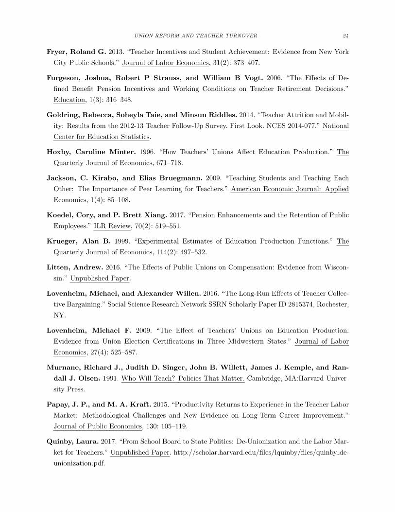
UNION REFORM AND TEACHER TURNOVER 24
Fryer, Roland G. 2013. “Teacher Incentives and Student Achievement: Evidence from New York
City Public Schools.” Journal of Labor Economics, 31(2): 373–407.
Furgeson, Joshua, Robert P Strauss, and William B Vogt. 2006. “The Effects of De-
fined Benefit Pension Incentives and Working Conditions on Teacher Retirement Decisions.”
Education, 1(3): 316–348.
Goldring, Rebecca, Soheyla Taie, and Minsun Riddles. 2014. “Teacher Attrition and Mobil-
ity: Results from the 2012-13 Teacher Follow-Up Survey. First Look. NCES 2014-077.” National
Center for Education Statistics.
Hoxby, Caroline Minter. 1996. “How Teachers’ Unions Affect Education Production.” The
Quarterly Journal of Economics, 671–718.
Jackson, C. Kirabo, and Elias Bruegmann. 2009. “Teaching Students and Teaching Each
Other: The Importance of Peer Learning for Teachers.” American Economic Journal: Applied
Economics, 1(4): 85–108.
Koedel, Cory, and P. Brett Xiang. 2017. “Pension Enhancements and the Retention of Public
Employees.” ILR Review, 70(2): 519–551.
Krueger, Alan B. 1999. “Experimental Estimates of Education Production Functions.” The
Quarterly Journal of Economics, 114(2): 497–532.
Litten, Andrew. 2016. “The Effects of Public Unions on Compensation: Evidence from Wiscon-
sin.” Unpublished Paper.
Lovenheim, Michael, and Alexander Willen. 2016. “The Long-Run Effects of Teacher Collec-
tive Bargaining.” Social Science Research Network SSRN Scholarly Paper ID 2815374, Rochester,
NY.
Lovenheim, Michael F. 2009. “The Effect of Teachers’ Unions on Education Production:
Evidence from Union Election Certifications in Three Midwestern States.” Journal of Labor
Economics, 27(4): 525–587.
Murnane, Richard J., Judith D. Singer, John B. Willett, James J. Kemple, and Ran-
dall J. Olsen. 1991. Who Will Teach? Policies That Matter. Cambridge, MA:Harvard Univer-
sity Press.
Papay, J. P., and M. A. Kraft. 2015. “Productivity Returns to Experience in the Teacher Labor
Market: Methodological Challenges and New Evidence on Long-Term Career Improvement.”
Journal of Public Economics, 130: 105–119.
Quinby, Laura. 2017. “From School Board to State Politics: De-Unionization and the Labor Mar-
ket for Teachers.” Unpublished Paper. http://scholar.harvard.edu/files/lquinby/files/quinby de-
unionization.pdf.
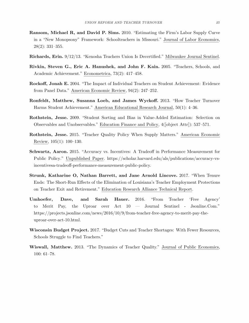
UNION REFORM AND TEACHER TURNOVER 25
Ransom, Michael R, and David P. Sims. 2010. “Estimating the Firm’s Labor Supply Curve
in a “New Monopsony” Framework: Schoolteachers in Missouri.” Journal of Labor Economics,
28(2): 331–355.
Richards, Erin. 9/12/13. “Kenosha Teachers Union Is Decertified.” Milwaukee Journal Sentinel.
Rivkin, Steven G., Eric A. Hanushek, and John F. Kain. 2005. “Teachers, Schools, and
Academic Achievement.” Econometrica, 73(2): 417–458.
Rockoff, Jonah E. 2004. “The Impact of Individual Teachers on Student Achievement: Evidence
from Panel Data.” American Economic Review, 94(2): 247–252.
Ronfeldt, Matthew, Susanna Loeb, and James Wyckoff. 2013. “How Teacher Turnover
Harms Student Achievement.” American Educational Research Journal, 50(1): 4–36.
Rothstein, Jesse. 2009. “Student Sorting and Bias in Value-Added Estimation: Selection on
Observables and Unobservables.” Education Finance and Policy, 4([object Attr]): 537–571.
Rothstein, Jesse. 2015. “Teacher Quality Policy When Supply Matters.” American Economic
Review, 105(1): 100–130.
Schwartz, Aaron. 2015. “Accuracy vs. Incentives: A Tradeoff in Performance Measurement for
Public Policy.” Unpublished Paper. https://scholar.harvard.edu/als/publications/accuracy-vs-
incentivesa-tradeoff-performance-measurement-public-policy.
Strunk, Katharine O, Nathan Barrett, and Jane Arnold Lincove. 2017. “When Tenure
Ends: The Short-Run Effects of the Elimination of Louisiana’s Teacher Employment Protections
on Teacher Exit and Retirement.” Education Research Alliance Technical Report.
Umhoefer, Dave, and Sarah Hauer. 2016. “From Teacher ‘Free Agency’
to Merit Pay, the Uproar over Act 10 — Journal Sentinel - Jsonline.Com.”
https://projects.jsonline.com/news/2016/10/9/from-teacher-free-agency-to-merit-pay-the-
uproar-over-act-10.html.
Wisconsin Budget Project. 2017. “Budget Cuts and Teacher Shortages: With Fewer Resources,
Schools Struggle to Find Teachers.”
Wiswall, Matthew. 2013. “The Dynamics of Teacher Quality.” Journal of Public Economics,
100: 61–78.
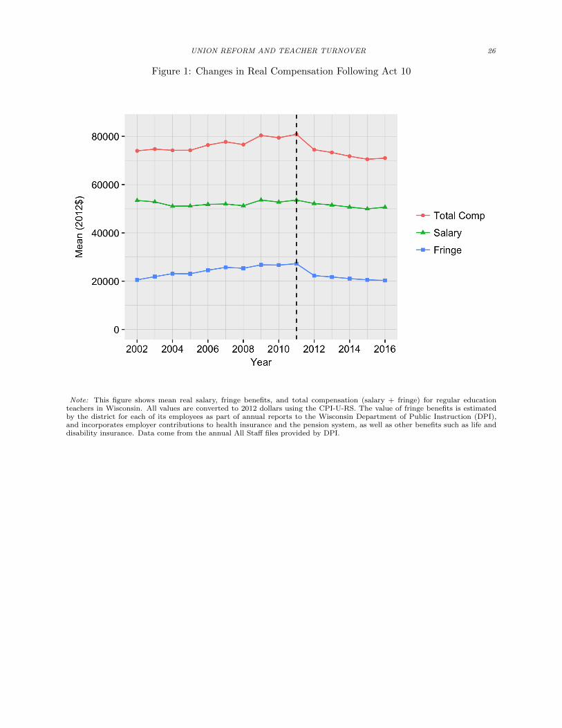
UNION REFORM AND TEACHER TURNOVER 26
Figure 1: Changes in Real Compensation Following Act 10
Note: This figure shows mean real salary, fringe benefits, and total compensation (salary + fringe) for regular educationteachers in Wisconsin. All values are converted to 2012 dollars using the CPI-U-RS. The value of fringe benefits is estimatedby the district for each of its employees as part of annual reports to the Wisconsin Department of Public Instruction (DPI),and incorporates employer contributions to health insurance and the pension system, as well as other benefits such as life anddisability insurance. Data come from the annual All Staff files provided by DPI.
UNION REFORM AND TEACHER TURNOVER 27
Figure 2
Note: This figure shows attrition rates by year and the corresponding 95% confidence intervals for regular education teachersin the Wisconsin public school system. Attrition rates are calculated using the All Staff files from the Wisconsin Departmentof Public Instruction. A teacher is said to have attrited between year t and year t+ 1 if they were a regular education teacheranywhere in the Wisconsin public schools in year t and were not a regular education teacher anywhere in the Wisconsin publicschools in year t + 1. See Section III.A for additional details on how attrition is calculated. The attrition rate plotted for agiven year represents the fraction of teachers who attrited following the school year ending with that year – for instance, theattrition rate for 2007 represents the fraction of teachers in the 2006-2007 school year who did not teach in 2007-2008.
Figure 3
Note: This figure shows attrition rates by year and the corresponding 95% confidence intervals for regular education teachersin the Wisconsin public school system. Separate series are shown for teachers above and below the minimum retirement ageof 55 in the relevant year. Attrition rates are calculated using the All Staff files from the Wisconsin Department of PublicInstruction. A teacher is said to have attrited between year t and year t+ 1 if they were a regular education teacher anywherein the Wisconsin public schools in year t and were not a regular education teacher anywhere in the Wisconsin public schoolsin year t+ 1. See Section III.A for additional details on how attrition is calculated. The attrition rate plotted for a given yearrepresents the fraction of teachers who attrited following the school year ending with that year – for instance, the attrition ratefor 2007 represents the fraction of teachers in the 2006-2007 school year who did not teach in 2007-2008.
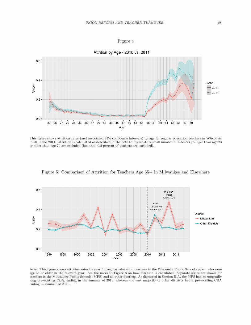
UNION REFORM AND TEACHER TURNOVER 28
Figure 4
This figure shows attrition rates (and associated 95% confidence intervals) by age for regular education teachers in Wisconsinin 2010 and 2011. Attrition is calculated as described in the note to Figure 3. A small number of teachers younger than age 23or older than age 70 are excluded (less than 0.2 percent of teachers are excluded).
Figure 5: Comparison of Attrition for Teachers Age 55+ in Milwaukee and Elsewhere
Note: This figure shows attrition rates by year for regular education teachers in the Wisconsin Public School system who wereage 55 or older in the relevant year. See the notes to Figure 3 on how attrition is calculated. Separate series are shown forteachers in the Milwaukee Public Schools (MPS) and all other districts. As discussed in Section II.A, the MPS had an unusuallylong pre-existing CBA, ending in the summer of 2013, whereas the vast majority of other districts had a pre-existing CBAending in summer of 2011.
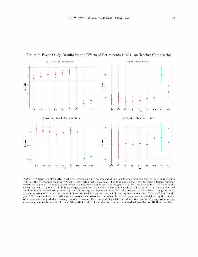
UNION REFORM AND TEACHER TURNOVER 29
Figure 6: Event Study Results for the Effects of Retirements in 2011 on Teacher Composition
(a) Average Experience (b) Fraction Novice
(c) Average Total Compensation (d) Student Teacher Ratios
Note: This figure displays OLS coefficient estimates and the associated 95% confidence intervals for the β1,τ in regression(1), i.e. the coefficients on frac retire2011 interacted with each year. The four panels show results using different outcomevariables. In panel a), the dependent variable is the fraction of teachers in the grade-level who are new to the Wisconsin publicschool system. In panel b), it is the average experience of teachers in the grade-level, and in panel c) it is the average realtotal compensation (salary + benefits). In column (4), the dependent variable is the student-teacher ratio at the grade-level,i.e. the number of students in the grade-level, divided by the number of full-time-equivalent teachers. The coefficient for theyear 2011 is normalized to 0. All standard errors are clustered at the school level, and regressions are weighted by the numberof students in the grade-level taking the WKCE exam. For comparability with the value-added results, the regression samplecontains grade-levels between 3rd and 5th grade for which I am able to construct value-added (see Section III.B for details).
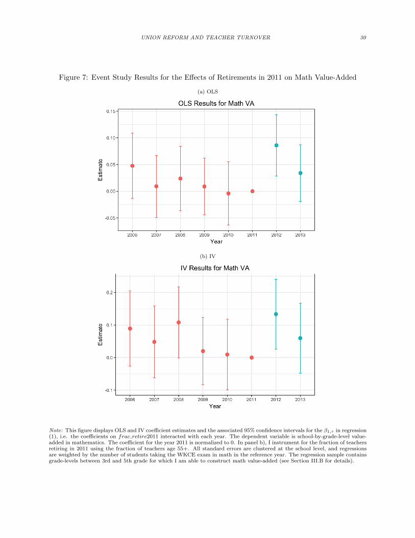
UNION REFORM AND TEACHER TURNOVER 30
Figure 7: Event Study Results for the Effects of Retirements in 2011 on Math Value-Added
(a) OLS
(b) IV
Note: This figure displays OLS and IV coefficient estimates and the associated 95% confidence intervals for the β1,τ in regression(1), i.e. the coefficients on frac retire2011 interacted with each year. The dependent variable is school-by-grade-level value-added in mathematics. The coefficient for the year 2011 is normalized to 0. In panel b), I instrument for the fraction of teachersretiring in 2011 using the fraction of teachers age 55+. All standard errors are clustered at the school level, and regressionsare weighted by the number of students taking the WKCE exam in math in the reference year. The regression sample containsgrade-levels between 3rd and 5th grade for which I am able to construct math value-added (see Section III.B for details).
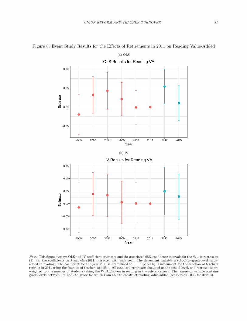
UNION REFORM AND TEACHER TURNOVER 31
Figure 8: Event Study Results for the Effects of Retirements in 2011 on Reading Value-Added
(a) OLS
(b) IV
Note: This figure displays OLS and IV coefficient estimates and the associated 95% confidence intervals for the β1,τ in regression(1), i.e. the coefficients on frac retire2011 interacted with each year. The dependent variable is school-by-grade-level value-added in reading. The coefficient for the year 2011 is normalized to 0. In panel b), I instrument for the fraction of teachersretiring in 2011 using the fraction of teachers age 55+. All standard errors are clustered at the school level, and regressions areweighted by the number of students taking the WKCE exam in reading in the reference year. The regression sample containsgrade-levels between 3rd and 5th grade for which I am able to construct reading value-added (see Section III.B for details).
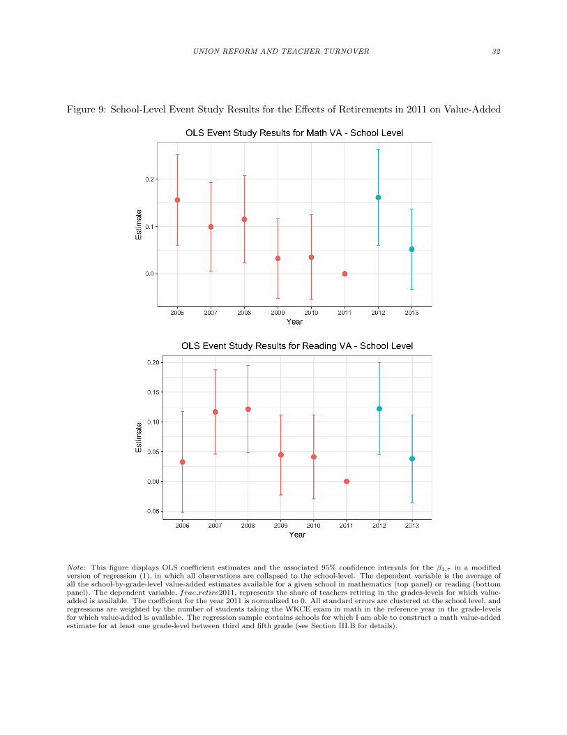
UNION REFORM AND TEACHER TURNOVER 32
Figure 9: School-Level Event Study Results for the Effects of Retirements in 2011 on Value-Added
Note: This figure displays OLS coefficient estimates and the associated 95% confidence intervals for the β1,τ in a modifiedversion of regression (1), in which all observations are collapsed to the school-level. The dependent variable is the average ofall the school-by-grade-level value-added estimates available for a given school in mathematics (top panel) or reading (bottompanel). The dependent variable, frac retire2011, represents the share of teachers retiring in the grades-levels for which value-added is available. The coefficient for the year 2011 is normalized to 0. All standard errors are clustered at the school level, andregressions are weighted by the number of students taking the WKCE exam in math in the reference year in the grade-levelsfor which value-added is available. The regression sample contains schools for which I am able to construct a math value-addedestimate for at least one grade-level between third and fifth grade (see Section III.B for details).
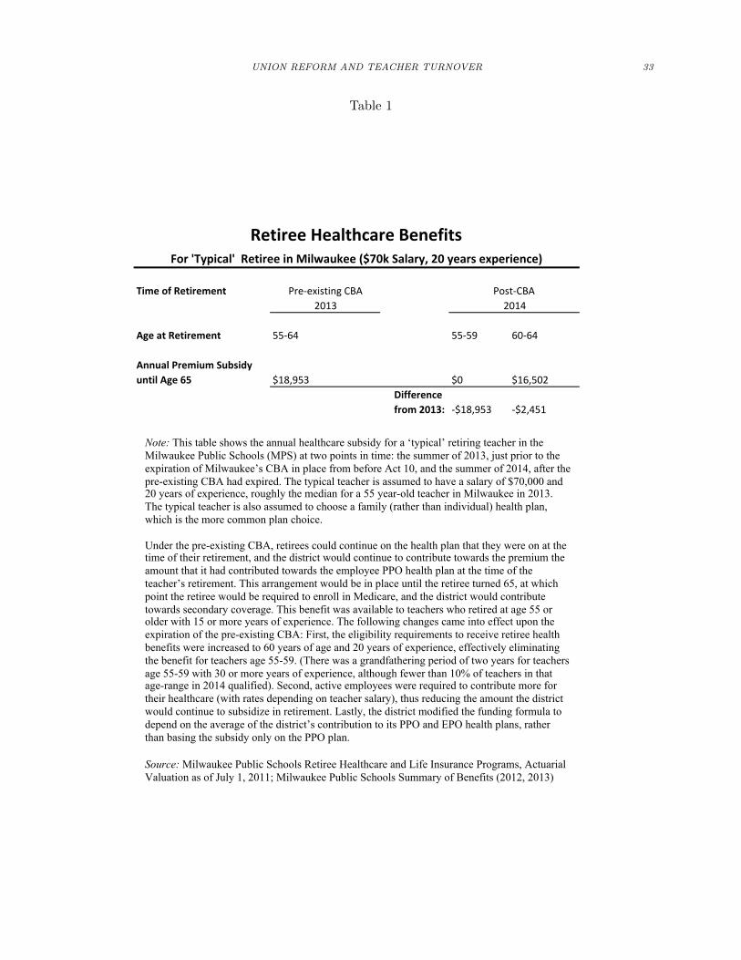
UNION REFORM AND TEACHER TURNOVER 33
Table 1
Time of Retirement Pre-‐existing CBA2013
Age at Retirement 55-‐64 55-‐59 60-‐64
Annual Premium Subsidy until Age 65 $18,953 $0 $16,502
Difference from 2013: -‐$18,953 -‐$2,451
Post-‐CBA2014
Retiree Healthcare BenefitsFor 'Typical' Retiree in Milwaukee ($70k Salary, 20 years experience)
Note: This table shows the annual healthcare subsidy for a ‘typical’ retiring teacher in the Milwaukee Public Schools (MPS) at two points in time: the summer of 2013, just prior to the expiration of Milwaukee’s CBA in place from before Act 10, and the summer of 2014, after the pre-existing CBA had expired. The typical teacher is assumed to have a salary of $70,000 and 20 years of experience, roughly the median for a 55 year-old teacher in Milwaukee in 2013. The typical teacher is also assumed to choose a family (rather than individual) health plan,which is the more common plan choice.
Under the pre-existing CBA, retirees could continue on the health plan that they were on at the time of their retirement, and the district would continue to contribute towards the premium the amount that it had contributed towards the employee PPO health plan at the time of the teacher’s retirement. This arrangement would be in place until the retiree turned 65, at which point the retiree would be required to enroll in Medicare, and the district would contribute towards secondary coverage. This benefit was available to teachers who retired at age 55 or older with 15 or more years of experience. The following changes came into effect upon the expiration of the pre-existing CBA: First, the eligibility requirements to receive retiree health benefits were increased to 60 years of age and 20 years of experience, effectively eliminating the benefit for teachers age 55-59. (There was a grandfathering period of two years for teachers age 55-59 with 30 or more years of experience, although fewer than 10% of teachers in that age-range in 2014 qualified). Second, active employees were required to contribute more for their healthcare (with rates depending on teacher salary), thus reducing the amount the district would continue to subsidize in retirement. Lastly, the district modified the funding formula to depend on the average of the district’s contribution to its PPO and EPO health plans, rather than basing the subsidy only on the PPO plan.
Source:Milwaukee Public Schools Retiree Healthcare and Life Insurance Programs, Actuarial Valuation as of July 1, 2011; Milwaukee Public Schools Summary of Benefits (2012, 2013)
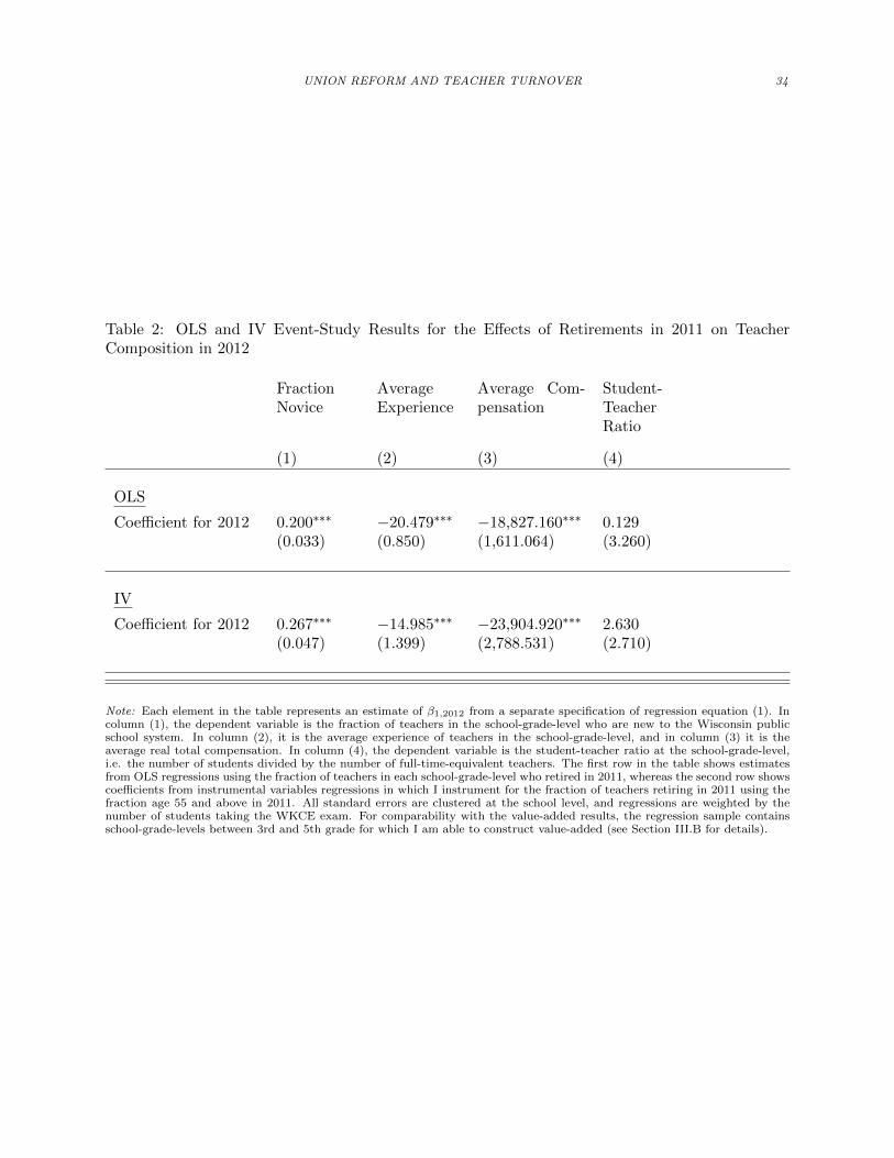
UNION REFORM AND TEACHER TURNOVER 34
Table 2: OLS and IV Event-Study Results for the Effects of Retirements in 2011 on TeacherComposition in 2012
FractionNovice
AverageExperience
Average Com-pensation
Student-TeacherRatio
(1) (2) (3) (4)
OLS
Coefficient for 2012 0.200∗∗∗ −20.479∗∗∗ −18,827.160∗∗∗ 0.129(0.033) (0.850) (1,611.064) (3.260)
IV
Coefficient for 2012 0.267∗∗∗ −14.985∗∗∗ −23,904.920∗∗∗ 2.630(0.047) (1.399) (2,788.531) (2.710)
Note: Each element in the table represents an estimate of β1,2012 from a separate specification of regression equation (1). Incolumn (1), the dependent variable is the fraction of teachers in the school-grade-level who are new to the Wisconsin publicschool system. In column (2), it is the average experience of teachers in the school-grade-level, and in column (3) it is theaverage real total compensation. In column (4), the dependent variable is the student-teacher ratio at the school-grade-level,i.e. the number of students divided by the number of full-time-equivalent teachers. The first row in the table shows estimatesfrom OLS regressions using the fraction of teachers in each school-grade-level who retired in 2011, whereas the second row showscoefficients from instrumental variables regressions in which I instrument for the fraction of teachers retiring in 2011 using thefraction age 55 and above in 2011. All standard errors are clustered at the school level, and regressions are weighted by thenumber of students taking the WKCE exam. For comparability with the value-added results, the regression sample containsschool-grade-levels between 3rd and 5th grade for which I am able to construct value-added (see Section III.B for details).
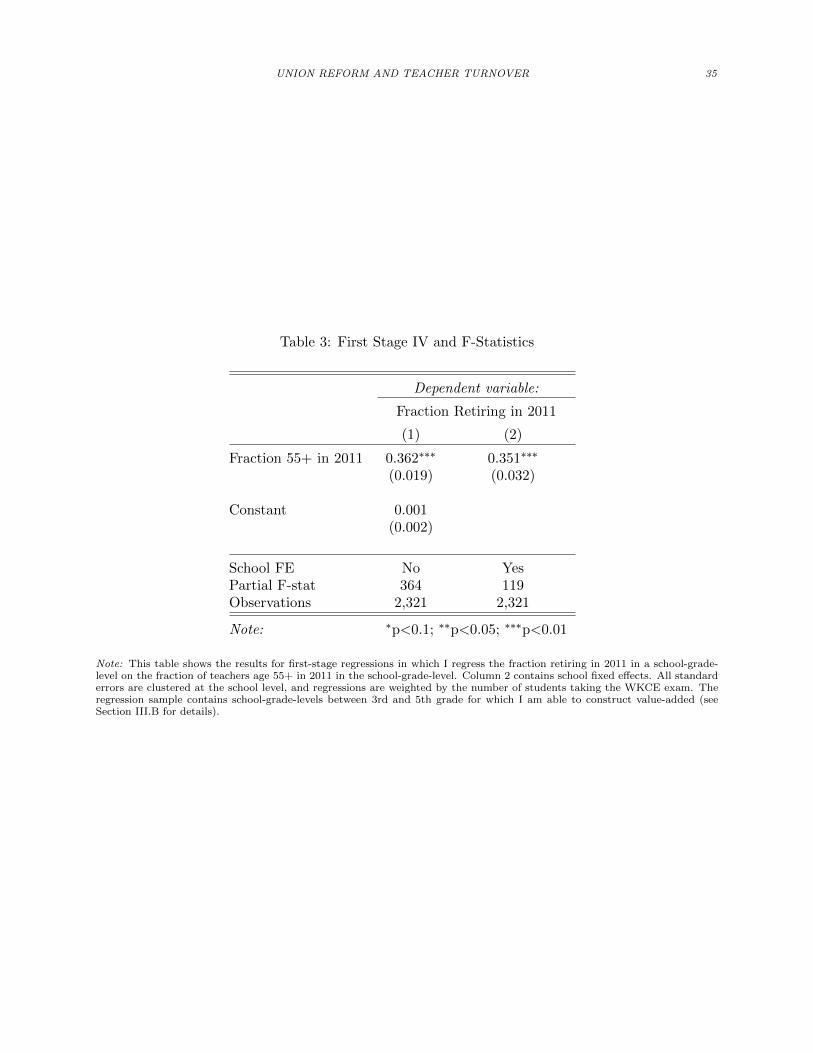
UNION REFORM AND TEACHER TURNOVER 35
Table 3: First Stage IV and F-Statistics
Dependent variable:
Fraction Retiring in 2011
(1) (2)
Fraction 55+ in 2011 0.362∗∗∗ 0.351∗∗∗
(0.019) (0.032)
Constant 0.001(0.002)
School FE No YesPartial F-stat 364 119Observations 2,321 2,321
Note: ∗p<0.1; ∗∗p<0.05; ∗∗∗p<0.01
Note: This table shows the results for first-stage regressions in which I regress the fraction retiring in 2011 in a school-grade-level on the fraction of teachers age 55+ in 2011 in the school-grade-level. Column 2 contains school fixed effects. All standarderrors are clustered at the school level, and regressions are weighted by the number of students taking the WKCE exam. Theregression sample contains school-grade-levels between 3rd and 5th grade for which I am able to construct value-added (seeSection III.B for details).
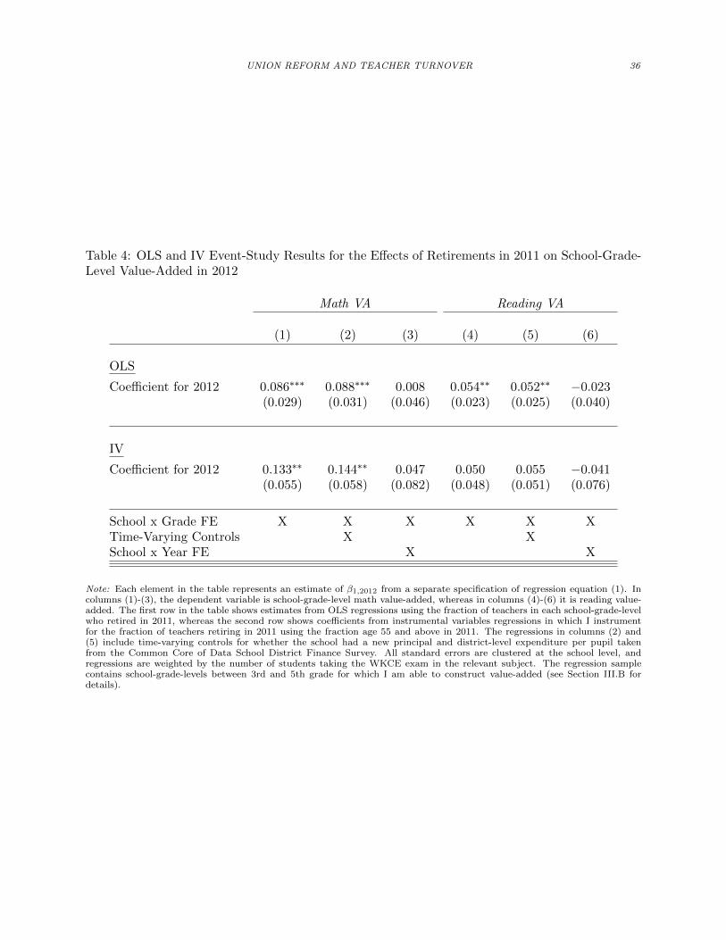
UNION REFORM AND TEACHER TURNOVER 36
Table 4: OLS and IV Event-Study Results for the Effects of Retirements in 2011 on School-Grade-Level Value-Added in 2012
Math VA Reading VA
(1) (2) (3) (4) (5) (6)
OLS
Coefficient for 2012 0.086∗∗∗ 0.088∗∗∗ 0.008 0.054∗∗ 0.052∗∗ −0.023(0.029) (0.031) (0.046) (0.023) (0.025) (0.040)
IV
Coefficient for 2012 0.133∗∗ 0.144∗∗ 0.047 0.050 0.055 −0.041(0.055) (0.058) (0.082) (0.048) (0.051) (0.076)
School x Grade FE X X X X X XTime-Varying Controls X XSchool x Year FE X X
Note: Each element in the table represents an estimate of β1,2012 from a separate specification of regression equation (1). Incolumns (1)-(3), the dependent variable is school-grade-level math value-added, whereas in columns (4)-(6) it is reading value-added. The first row in the table shows estimates from OLS regressions using the fraction of teachers in each school-grade-levelwho retired in 2011, whereas the second row shows coefficients from instrumental variables regressions in which I instrumentfor the fraction of teachers retiring in 2011 using the fraction age 55 and above in 2011. The regressions in columns (2) and(5) include time-varying controls for whether the school had a new principal and district-level expenditure per pupil takenfrom the Common Core of Data School District Finance Survey. All standard errors are clustered at the school level, andregressions are weighted by the number of students taking the WKCE exam in the relevant subject. The regression samplecontains school-grade-levels between 3rd and 5th grade for which I am able to construct value-added (see Section III.B fordetails).
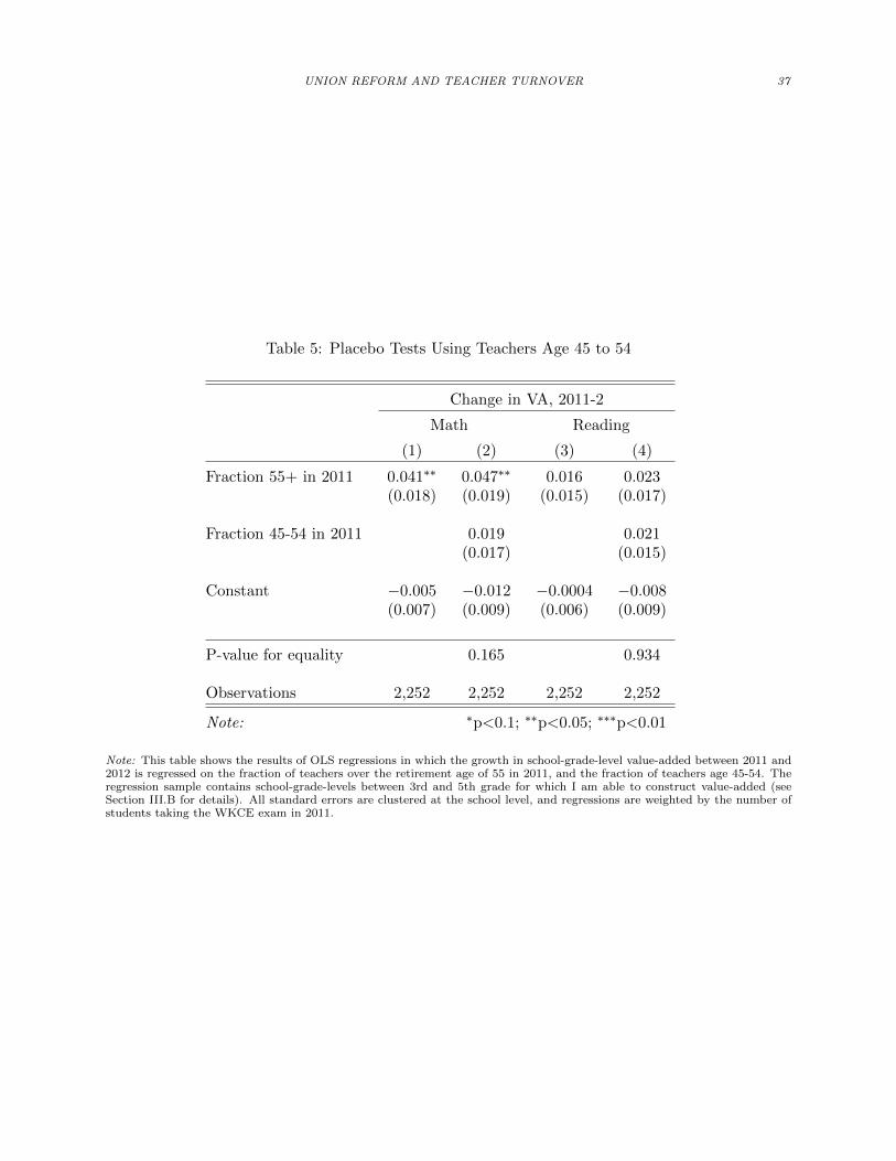
UNION REFORM AND TEACHER TURNOVER 37
Table 5: Placebo Tests Using Teachers Age 45 to 54
Change in VA, 2011-2
Math Reading
(1) (2) (3) (4)
Fraction 55+ in 2011 0.041∗∗ 0.047∗∗ 0.016 0.023(0.018) (0.019) (0.015) (0.017)
Fraction 45-54 in 2011 0.019 0.021(0.017) (0.015)
Constant −0.005 −0.012 −0.0004 −0.008(0.007) (0.009) (0.006) (0.009)
P-value for equality 0.165 0.934
Observations 2,252 2,252 2,252 2,252
Note: ∗p<0.1; ∗∗p<0.05; ∗∗∗p<0.01
Note: This table shows the results of OLS regressions in which the growth in school-grade-level value-added between 2011 and2012 is regressed on the fraction of teachers over the retirement age of 55 in 2011, and the fraction of teachers age 45-54. Theregression sample contains school-grade-levels between 3rd and 5th grade for which I am able to construct value-added (seeSection III.B for details). All standard errors are clustered at the school level, and regressions are weighted by the number ofstudents taking the WKCE exam in 2011.
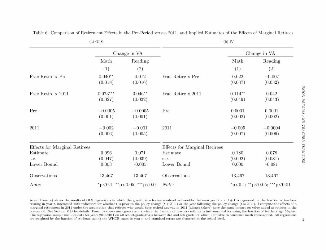
UNIO
NREFORM
AND
TEACHER
TURNOVER
38
Table 6: Comparison of Retirement Effects in the Pre-Period versus 2011, and Implied Estimates of the Effects of Marginal Retirees
(a) OLS
Change in VA
Math Reading
(1) (2)
Frac Retire x Pre 0.040∗∗ 0.012(0.018) (0.016)
Frac Retire x 2011 0.073∗∗∗ 0.046∗∗
(0.027) (0.022)
Pre −0.0005 −0.0005(0.001) (0.001)
2011 −0.002 −0.001(0.006) (0.005)
Effects for Marginal RetireesEstimate 0.096 0.071s.e. (0.047) (0.039)Lower Bound 0.003 -0.005
Observations 13,467 13,467
Note: ∗p<0.1; ∗∗p<0.05; ∗∗∗p<0.01
(b) IV
Change in VA
Math Reading
(1) (2)
Frac Retire x Pre 0.022 −0.007(0.037) (0.032)
Frac Retire x 2011 0.114∗∗ 0.042(0.049) (0.043)
Pre 0.0001 0.0001(0.002) (0.002)
2011 −0.005 −0.0004(0.007) (0.006)
Effects for Marginal RetireesEstimate 0.180 0.078s.e. (0.092) (0.081)Lower Bound 0.000 -0.081
Observations 13,467 13,467
Note: ∗p<0.1; ∗∗p<0.05; ∗∗∗p<0.01
Note: Panel a) shows the results of OLS regressions in which the growth in school-grade-level value-added between year t and t + 1 is regressed on the fraction of teachersretiring in year t, interacted with indicators for whether t is prior to the policy change (t < 2011) or the year following the policy change (t = 2011). I compute the effects of amarginal retirement in 2011 under the assumption that retirees who would have retired anyway in 2011 (always-takers) have the same impact on value-added as retirees in thepre-period. See Section V.D for details. Panel b) shows analogous results where the fraction of teachers retiring is instrumented for using the fraction of teachers age 55-plus.The regression sample includes data for years 2006-2011 on all school-grade-levels between 3rd and 5th grade for which I am able to construct math value-added. All regressionsare weighted by the fraction of students taking the WKCE exam in year t, and standard errors are clustered at the school level.
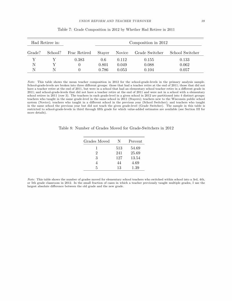
UNION REFORM AND TEACHER TURNOVER 39
Table 7: Grade Composition in 2012 by Whether Had Retiree in 2011
Had Retiree in: Composition in 2012
Grade? School? Frac Retired Stayer Novice Grade Switcher School Switcher
Y Y 0.383 0.6 0.112 0.155 0.133N Y 0 0.801 0.049 0.088 0.062N N 0 0.786 0.053 0.104 0.057
Note: This table shows the mean teacher composition in 2012 for the school-grade-levels in the primary analysis sample.School-grade-levels are broken into three different groups: those that had a teacher retire at the end of 2011; those that did nothave a teacher retire at the end of 2011, but were in a school that had an elementary school teacher retire in a different grade in2011; and school-grade-levels that did not have a teacher retire at the end of 2011 and were not in a school with a elementaryschool retiree in 2011 (row 3). The teachers in each grade-level in a given school in 2012 are partitioned into 4 distinct groups:teachers who taught in the same grade-level in the same school in 2011 (Stayers); teachers new to the Wisconsin public schoolsystem (Novice); teachers who taught in a different school in the previous year (School Switcher); and teachers who taughtin the same school the previous year but did not teach the given grade-level (Grade Switcher). The sample in this table isrestricted to school-grade-levels in third through fifth grade for which value-added estimates are available (see Section III formore details).
Table 8: Number of Grades Moved for Grade-Switchers in 2012
Grades Moved N Percent
1 513 54.692 241 25.693 127 13.544 44 4.695 13 1.39
Note: This table shows the number of grades moved for elementary school teachers who switched within school into a 3rd, 4th,or 5th grade classroom in 2012. In the small fraction of cases in which a teacher previously taught multiple grades, I use thelargest absolute difference between the old grade and the new grade.
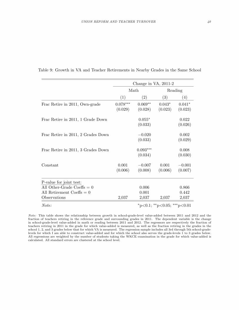
UNION REFORM AND TEACHER TURNOVER 40
Table 9: Growth in VA and Teacher Retirements in Nearby Grades in the Same School
Change in VA, 2011-2
Math Reading
(1) (2) (3) (4)
Frac Retire in 2011, Own-grade 0.078∗∗∗ 0.069∗∗ 0.043∗ 0.041∗
(0.029) (0.028) (0.023) (0.023)
Frac Retire in 2011, 1 Grade Down 0.055∗ 0.022(0.033) (0.026)
Frac Retire in 2011, 2 Grades Down −0.020 0.002(0.033) (0.029)
Frac Retire in 2011, 3 Grades Down 0.093∗∗∗ 0.008(0.034) (0.030)
Constant 0.001 −0.007 0.001 −0.001(0.006) (0.008) (0.006) (0.007)
P-value for joint test:All Other-Grade Coeffs = 0 0.006 0.866All Retirement Coeffs = 0 0.001 0.442Observations 2,037 2,037 2,037 2,037
Note: ∗p<0.1; ∗∗p<0.05; ∗∗∗p<0.01
Note: This table shows the relationship between growth in school-grade-level value-added between 2011 and 2012 and thefraction of teachers retiring in the reference grade and surrounding grades in 2011. The dependent variable is the changein school-grade-level value-added in math or reading between 2011 and 2012. The regressors are respectively the fraction ofteachers retiring in 2011 in the grade for which value-added is measured, as well as the fraction retiring in the grades in theschool 1, 2, and 3 grades below that for which VA is measured. The regression sample includes all 3rd through 5th school-grade-levels for which I am able to construct value-added and for which the school also serves the grade-levels 1 to 3 grades below.All regressions are weighted by the number of students taking the WKCE examination in the grade for which value-added iscalculated. All standard errors are clustered at the school level.
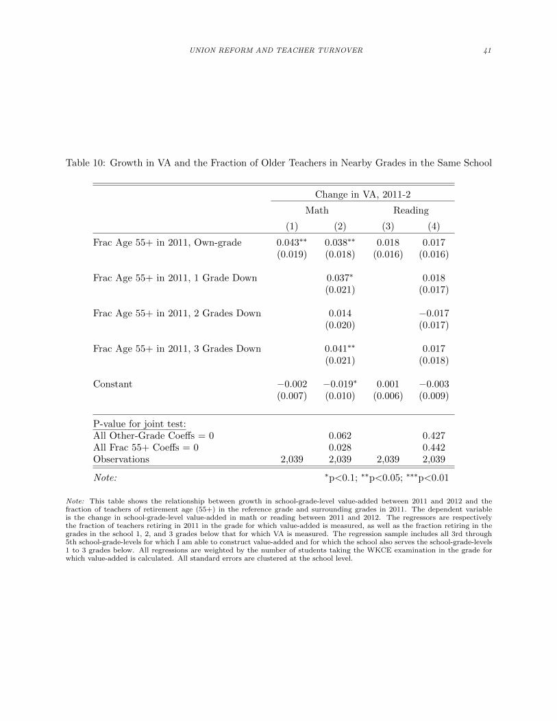
UNION REFORM AND TEACHER TURNOVER 41
Table 10: Growth in VA and the Fraction of Older Teachers in Nearby Grades in the Same School
Change in VA, 2011-2
Math Reading
(1) (2) (3) (4)
Frac Age 55+ in 2011, Own-grade 0.043∗∗ 0.038∗∗ 0.018 0.017(0.019) (0.018) (0.016) (0.016)
Frac Age 55+ in 2011, 1 Grade Down 0.037∗ 0.018(0.021) (0.017)
Frac Age 55+ in 2011, 2 Grades Down 0.014 −0.017(0.020) (0.017)
Frac Age 55+ in 2011, 3 Grades Down 0.041∗∗ 0.017(0.021) (0.018)
Constant −0.002 −0.019∗ 0.001 −0.003(0.007) (0.010) (0.006) (0.009)
P-value for joint test:All Other-Grade Coeffs = 0 0.062 0.427All Frac 55+ Coeffs = 0 0.028 0.442Observations 2,039 2,039 2,039 2,039
Note: ∗p<0.1; ∗∗p<0.05; ∗∗∗p<0.01
Note: This table shows the relationship between growth in school-grade-level value-added between 2011 and 2012 and thefraction of teachers of retirement age (55+) in the reference grade and surrounding grades in 2011. The dependent variableis the change in school-grade-level value-added in math or reading between 2011 and 2012. The regressors are respectivelythe fraction of teachers retiring in 2011 in the grade for which value-added is measured, as well as the fraction retiring in thegrades in the school 1, 2, and 3 grades below that for which VA is measured. The regression sample includes all 3rd through5th school-grade-levels for which I am able to construct value-added and for which the school also serves the school-grade-levels1 to 3 grades below. All regressions are weighted by the number of students taking the WKCE examination in the grade forwhich value-added is calculated. All standard errors are clustered at the school level.
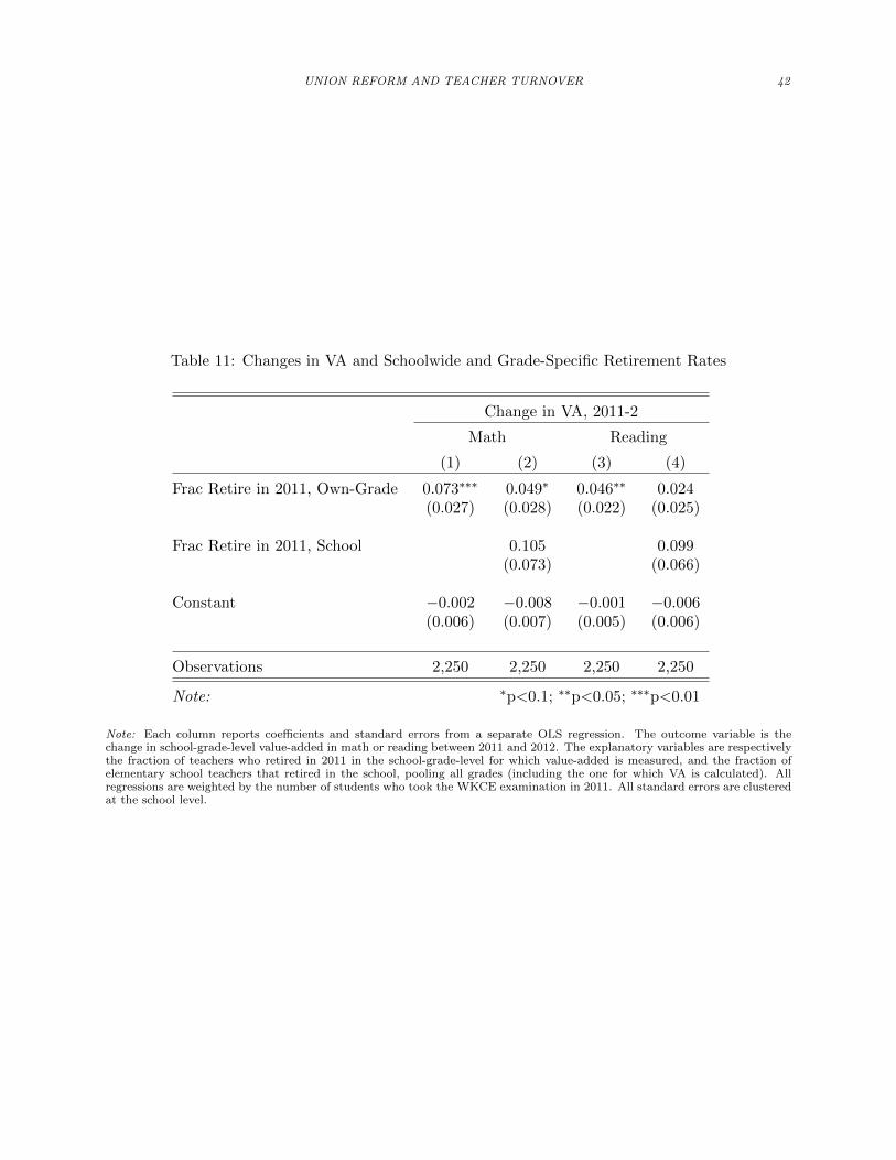
UNION REFORM AND TEACHER TURNOVER 42
Table 11: Changes in VA and Schoolwide and Grade-Specific Retirement Rates
Change in VA, 2011-2
Math Reading
(1) (2) (3) (4)
Frac Retire in 2011, Own-Grade 0.073∗∗∗ 0.049∗ 0.046∗∗ 0.024(0.027) (0.028) (0.022) (0.025)
Frac Retire in 2011, School 0.105 0.099(0.073) (0.066)
Constant −0.002 −0.008 −0.001 −0.006(0.006) (0.007) (0.005) (0.006)
Observations 2,250 2,250 2,250 2,250
Note: ∗p<0.1; ∗∗p<0.05; ∗∗∗p<0.01
Note: Each column reports coefficients and standard errors from a separate OLS regression. The outcome variable is thechange in school-grade-level value-added in math or reading between 2011 and 2012. The explanatory variables are respectivelythe fraction of teachers who retired in 2011 in the school-grade-level for which value-added is measured, and the fraction ofelementary school teachers that retired in the school, pooling all grades (including the one for which VA is calculated). Allregressions are weighted by the number of students who took the WKCE examination in 2011. All standard errors are clusteredat the school level.
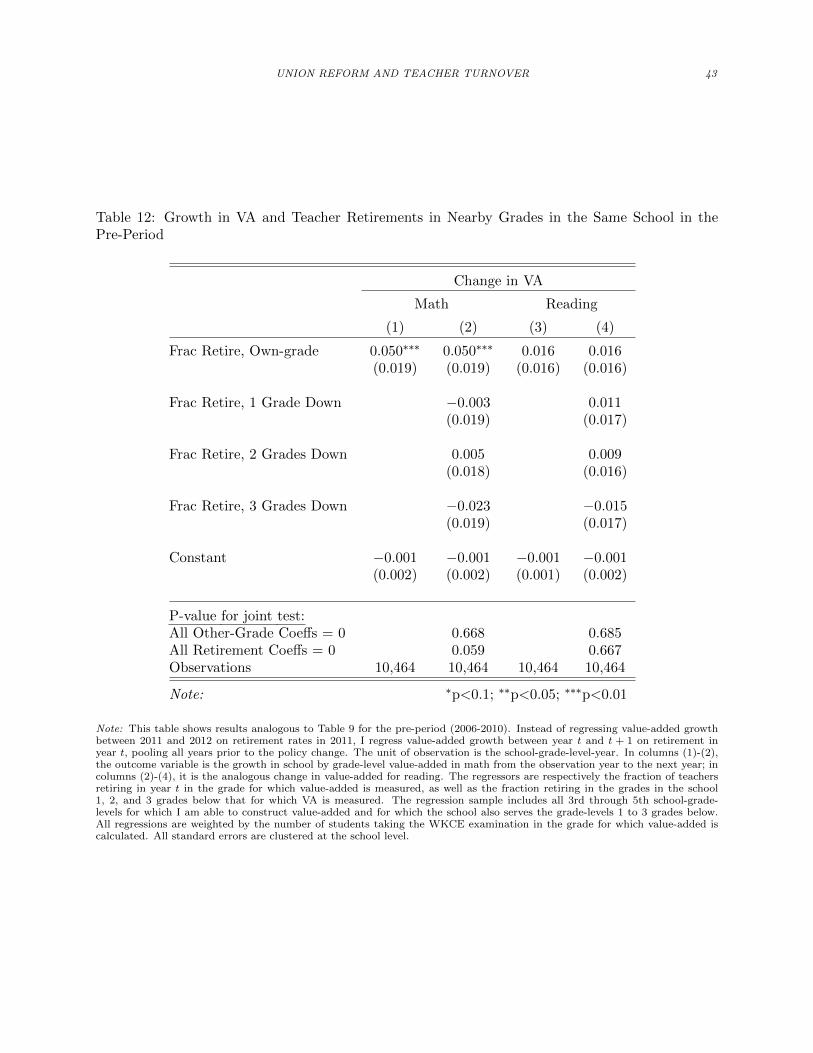
UNION REFORM AND TEACHER TURNOVER 43
Table 12: Growth in VA and Teacher Retirements in Nearby Grades in the Same School in thePre-Period
Change in VA
Math Reading
(1) (2) (3) (4)
Frac Retire, Own-grade 0.050∗∗∗ 0.050∗∗∗ 0.016 0.016(0.019) (0.019) (0.016) (0.016)
Frac Retire, 1 Grade Down −0.003 0.011(0.019) (0.017)
Frac Retire, 2 Grades Down 0.005 0.009(0.018) (0.016)
Frac Retire, 3 Grades Down −0.023 −0.015(0.019) (0.017)
Constant −0.001 −0.001 −0.001 −0.001(0.002) (0.002) (0.001) (0.002)
P-value for joint test:All Other-Grade Coeffs = 0 0.668 0.685All Retirement Coeffs = 0 0.059 0.667Observations 10,464 10,464 10,464 10,464
Note: ∗p<0.1; ∗∗p<0.05; ∗∗∗p<0.01
Note: This table shows results analogous to Table 9 for the pre-period (2006-2010). Instead of regressing value-added growthbetween 2011 and 2012 on retirement rates in 2011, I regress value-added growth between year t and t + 1 on retirement inyear t, pooling all years prior to the policy change. The unit of observation is the school-grade-level-year. In columns (1)-(2),the outcome variable is the growth in school by grade-level value-added in math from the observation year to the next year; incolumns (2)-(4), it is the analogous change in value-added for reading. The regressors are respectively the fraction of teachersretiring in year t in the grade for which value-added is measured, as well as the fraction retiring in the grades in the school1, 2, and 3 grades below that for which VA is measured. The regression sample includes all 3rd through 5th school-grade-levels for which I am able to construct value-added and for which the school also serves the grade-levels 1 to 3 grades below.All regressions are weighted by the number of students taking the WKCE examination in the grade for which value-added iscalculated. All standard errors are clustered at the school level.
UNION REFORM AND TEACHER TURNOVER 44
Appendix
A1. VARC Value-Added
As discussed in Section III.B, in my primary analysis I use a school-grade-level value-added
metric derived from school-grade-year level means on the WKCE exam. In this section, I reproduce
the main event-study results from Section V.C using an alternative measure of school-grade-level
value-added, constructed by the Wisconsin Value-Added Research Center (VARC) for internal use
by DPI.
Recall from Section III.B that the VARC value-added have both advantages and disadvantages
relative to the value-added metric used in the primary analysis. The main advantage of the VARC
value-added is that it covers a more complete set of school-grade levels than the primary analysis
VA (Appendix Table A2). The most severe disadvantage of the VARC value-added measures is that
they have had complex shrinkage procedure applied to them which cannot be reversed given the
information available to me. It is problematic to use shrunk measures of value-added as an outcome
variable since they will typically change less than one-for-one with changes in true effectiveness,
and thus we would expect the results to be attenuated towards zero (see Schwartz, 2015 for a
discussion). In addition, the control variables used by VARC vary somewhat across years, and for
some years VARC reports a value-added metric in the unit of student test scores, whereas in other
years they report only a z-score of the school-grade-level value-added.
To address the inconsistencies in units across years, I convert of all of the VARC value-added
estimates to have mean 0 and standard deviation 1 within each grade in each year. To some
extent, this also addresses the issue of shrinkage, since if the same shrinkage factor were applied
to the value-added for all school-grade levels, then the z-scores of the shrunk value-added would
be equivalent to the z-scores of the unshrunk value-added. However, this procedure does not fully
reverse the shrinkage procedure since in reality some school-grade levels are larger than others or
have noisier test scores, and thus the shrinkage factors will not be the same across school-grade
levels.
In order to make the results for the VARC sample as comparable as possible to the primary
analysis value-added measure, I also convert the value-added metric used in the primary analysis
(which is in z-scores of the student test score distribution) to have mean 0 and standard deviation 1
within each grade in each year. I then re-run my main analysis using i) the primary analysis value-
added standardized as above, ii) the standardized VARC value-added metric on the full sample of
third to fifth grade school-grade units, and iii) the standardized VARC value-added metric on the
sub-sample of third to fifth grade school-grade units used in the primary analysis. This allows us to
assess how sensitive the results are to both changes in the value-added metric as well as the sample
used.
Figures A1 to A4 respectively show the OLS and IV event study results for math, and the OLS
and IV event study results for reading for each of the three specifications discussed in the preceding
UNION REFORM AND TEACHER TURNOVER 45
paragraph. For math, both the OLS and IV results are quantitatively and qualitatively quite similar
across specifications. The OLS results for reading also follow similar patterns, although when using
the full VARC sample the coefficient for 2012 is somewhat smaller and no longer statistically
significant. When using the IV strategy for reading, the coefficient for 2012 flips sign when using
the VARC VA, although in none of the specifications is the coefficient significant. On the whole, the
event study results are fairly similar across specifications, particularly in math, where the results
are stronger.
As mentioned in Section V.E, however, the results of the placebo tests using teachers near
retirement age are less consistent across specifications (Table A3). In particular, while the coefficient
for the placebo group is not significant and smaller than that for retirees in the primary analysis,
in a number of cases the placebo coefficient is significant when using the VARC value-added. The
results for the VARC sample thus raise some concern that the observed increases in value-added
are driven by other factors correlated with the pre-existing age distribution.
A2. Appendix Tables and Figures
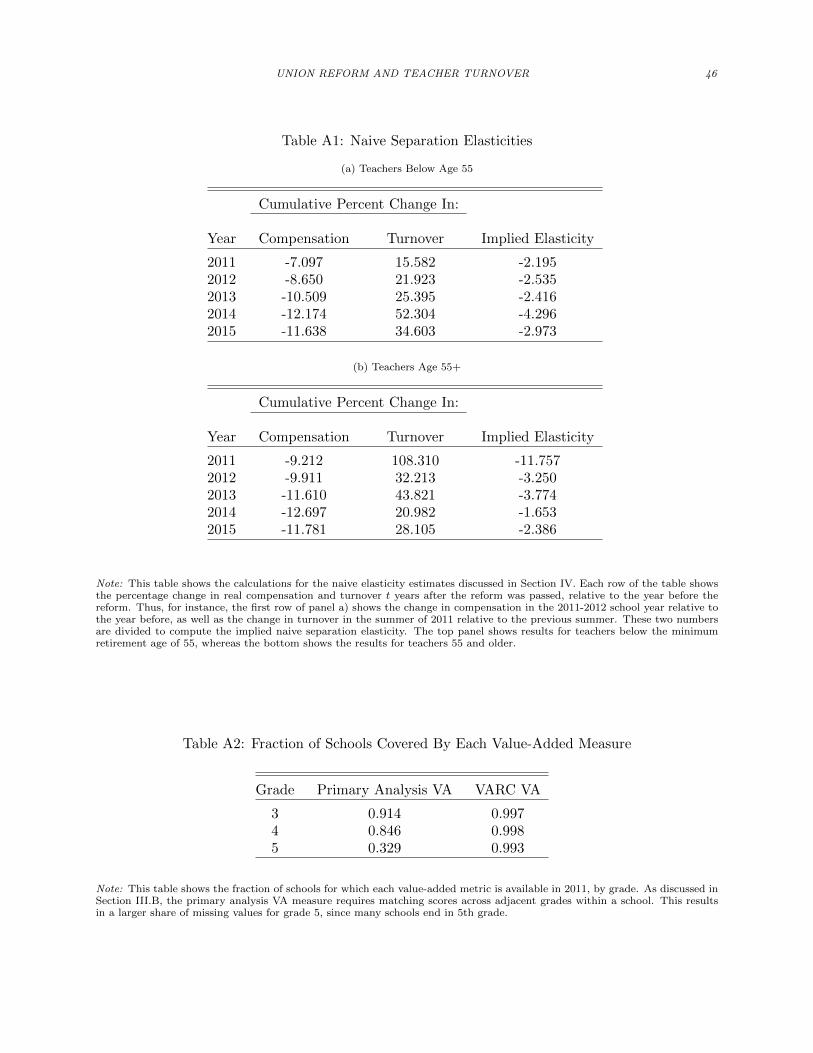
UNION REFORM AND TEACHER TURNOVER 46
Table A1: Naive Separation Elasticities
(a) Teachers Below Age 55
Cumulative Percent Change In:
Year Compensation Turnover Implied Elasticity
2011 -7.097 15.582 -2.1952012 -8.650 21.923 -2.5352013 -10.509 25.395 -2.4162014 -12.174 52.304 -4.2962015 -11.638 34.603 -2.973
(b) Teachers Age 55+
Cumulative Percent Change In:
Year Compensation Turnover Implied Elasticity
2011 -9.212 108.310 -11.7572012 -9.911 32.213 -3.2502013 -11.610 43.821 -3.7742014 -12.697 20.982 -1.6532015 -11.781 28.105 -2.386
Note: This table shows the calculations for the naive elasticity estimates discussed in Section IV. Each row of the table showsthe percentage change in real compensation and turnover t years after the reform was passed, relative to the year before thereform. Thus, for instance, the first row of panel a) shows the change in compensation in the 2011-2012 school year relative tothe year before, as well as the change in turnover in the summer of 2011 relative to the previous summer. These two numbersare divided to compute the implied naive separation elasticity. The top panel shows results for teachers below the minimumretirement age of 55, whereas the bottom shows the results for teachers 55 and older.
Table A2: Fraction of Schools Covered By Each Value-Added Measure
Grade Primary Analysis VA VARC VA
3 0.914 0.9974 0.846 0.9985 0.329 0.993
Note: This table shows the fraction of schools for which each value-added metric is available in 2011, by grade. As discussed inSection III.B, the primary analysis VA measure requires matching scores across adjacent grades within a school. This resultsin a larger share of missing values for grade 5, since many schools end in 5th grade.
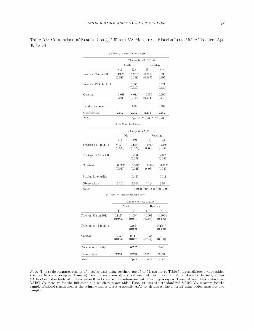
UNION REFORM AND TEACHER TURNOVER 47
Table A3: Comparison of Results Using Different VA Measures - Placebo Tests Using Teachers Age45 to 54
(a) Primary Analysis VA and Sample
Change in VA, 2011-2
Math Reading
(1) (2) (3) (4)
Fraction 55+ in 2011 0.198∗∗ 0.229∗∗∗ 0.096 0.136(0.082) (0.088) (0.087) (0.095)
Fraction 45-54 in 2011 0.096 0.121(0.080) (0.084)
Constant −0.048 −0.082∗ −0.056 −0.099∗∗
(0.031) (0.044) (0.034) (0.049)
P-value for equality 0.16 0.882
Observations 2,252 2,252 2,252 2,252
Note: ∗p<0.1; ∗∗p<0.05; ∗∗∗p<0.01
(b) VARC VA, Full Sample
Change in VA, 2011-2
Math Reading
(1) (2) (3) (4)
Fraction 55+ in 2011 0.127∗ 0.156∗∗ −0.094 −0.034(0.073) (0.078) (0.081) (0.088)
Fraction 45-54 in 2011 0.091 0.186∗∗
(0.078) (0.086)
Constant −0.052∗ −0.084∗∗ −0.024 −0.090∗
(0.030) (0.041) (0.034) (0.049)
P-value for equality 0.459 0.018
Observations 3,104 3,104 3,104 3,104
Note: ∗p<0.1; ∗∗p<0.05; ∗∗∗p<0.01
(c) VARC VA, Primary Analysis Sample
Change in VA, 2011-2
Math Reading
(1) (2) (3) (4)
Fraction 55+ in 2011 0.147∗ 0.200∗∗ −0.067 −0.0004(0.085) (0.091) (0.097) (0.106)
Fraction 45-54 in 2011 0.166∗ 0.205∗∗
(0.089) (0.100)
Constant −0.059∗ −0.117∗∗ −0.038 −0.110∗
(0.034) (0.047) (0.041) (0.058)
P-value for equality 0.737 0.06
Observations 2,250 2,250 2,250 2,250
Note: ∗p<0.1; ∗∗p<0.05; ∗∗∗p<0.01
Note: This table compares results of placebo tests using teachers age 45 to 54, similar to Table 5, across different value-addedspecifications and samples. Panel a) uses the same sample and value-added metric as the main analysis in the text, exceptVA has been standardized to have mean 0 and standard deviation one within each grade-year. Panel b) uses the standardizedVARC VA measure for the full sample in which it is available. Panel c) uses the standardized VARC VA measure for thesample of school-grades used in the primary analysis. See Appendix A.A1 for details on the different value-added measures andsamples.
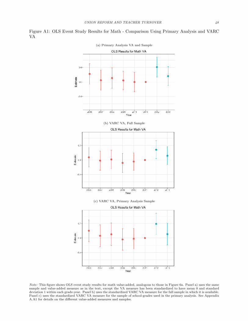
UNION REFORM AND TEACHER TURNOVER 48
Figure A1: OLS Event Study Results for Math - Comparison Using Primary Analysis and VARCVA
(a) Primary Analysis VA and Sample
(b) VARC VA, Full Sample
(c) VARC VA, Primary Analysis Sample
Note: This figure shows OLS event study results for math value-added, analogous to those in Figure 6a. Panel a) uses the samesample and value-added measure as in the text, except the VA measure has been standardized to have mean 0 and standarddeviation 1 within each grade-year. Panel b) uses the standardized VARC VA measure for the full sample in which it is available.Panel c) uses the standardized VARC VA measure for the sample of school-grades used in the primary analysis. See AppendixA.A1 for details on the different value-added measures and samples.
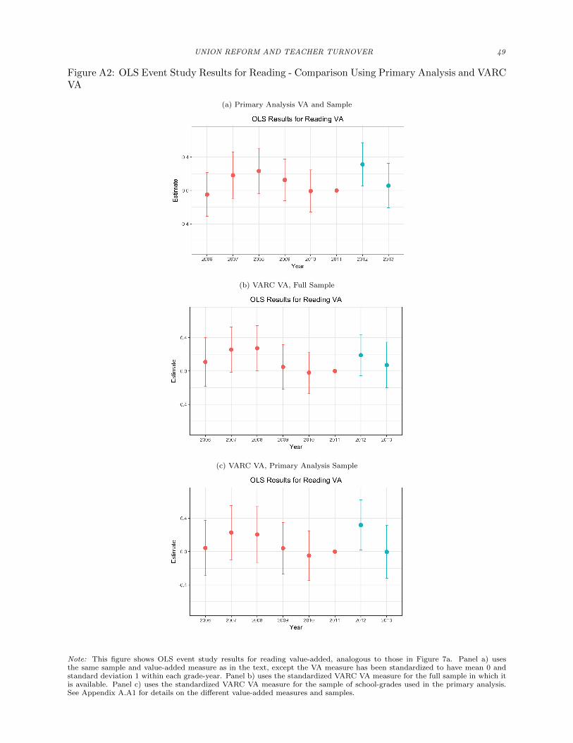
UNION REFORM AND TEACHER TURNOVER 49
Figure A2: OLS Event Study Results for Reading - Comparison Using Primary Analysis and VARCVA
(a) Primary Analysis VA and Sample
(b) VARC VA, Full Sample
(c) VARC VA, Primary Analysis Sample
Note: This figure shows OLS event study results for reading value-added, analogous to those in Figure 7a. Panel a) usesthe same sample and value-added measure as in the text, except the VA measure has been standardized to have mean 0 andstandard deviation 1 within each grade-year. Panel b) uses the standardized VARC VA measure for the full sample in which itis available. Panel c) uses the standardized VARC VA measure for the sample of school-grades used in the primary analysis.See Appendix A.A1 for details on the different value-added measures and samples.
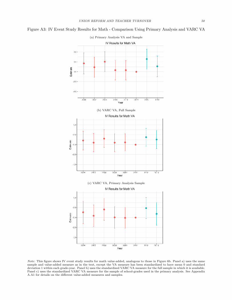
UNION REFORM AND TEACHER TURNOVER 50
Figure A3: IV Event Study Results for Math - Comparison Using Primary Analysis and VARC VA
(a) Primary Analysis VA and Sample
(b) VARC VA, Full Sample
(c) VARC VA, Primary Analysis Sample
Note: This figure shows IV event study results for math value-added, analogous to those in Figure 6b. Panel a) uses the samesample and value-added measure as in the text, except the VA measure has been standardized to have mean 0 and standarddeviation 1 within each grade-year. Panel b) uses the standardized VARC VA measure for the full sample in which it is available.Panel c) uses the standardized VARC VA measure for the sample of school-grades used in the primary analysis. See AppendixA.A1 for details on the different value-added measures and samples.
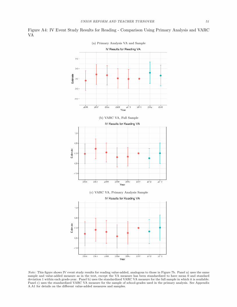
UNION REFORM AND TEACHER TURNOVER 51
Figure A4: IV Event Study Results for Reading - Comparison Using Primary Analysis and VARCVA
(a) Primary Analysis VA and Sample
(b) VARC VA, Full Sample
(c) VARC VA, Primary Analysis Sample
Note: This figure shows IV event study results for reading value-added, analogous to those in Figure 7b. Panel a) uses the samesample and value-added measure as in the text, except the VA measure has been standardized to have mean 0 and standarddeviation 1 within each grade-year. Panel b) uses the standardized VARC VA measure for the full sample in which it is available.Panel c) uses the standardized VARC VA measure for the sample of school-grades used in the primary analysis. See AppendixA.A1 for details on the different value-added measures and samples.
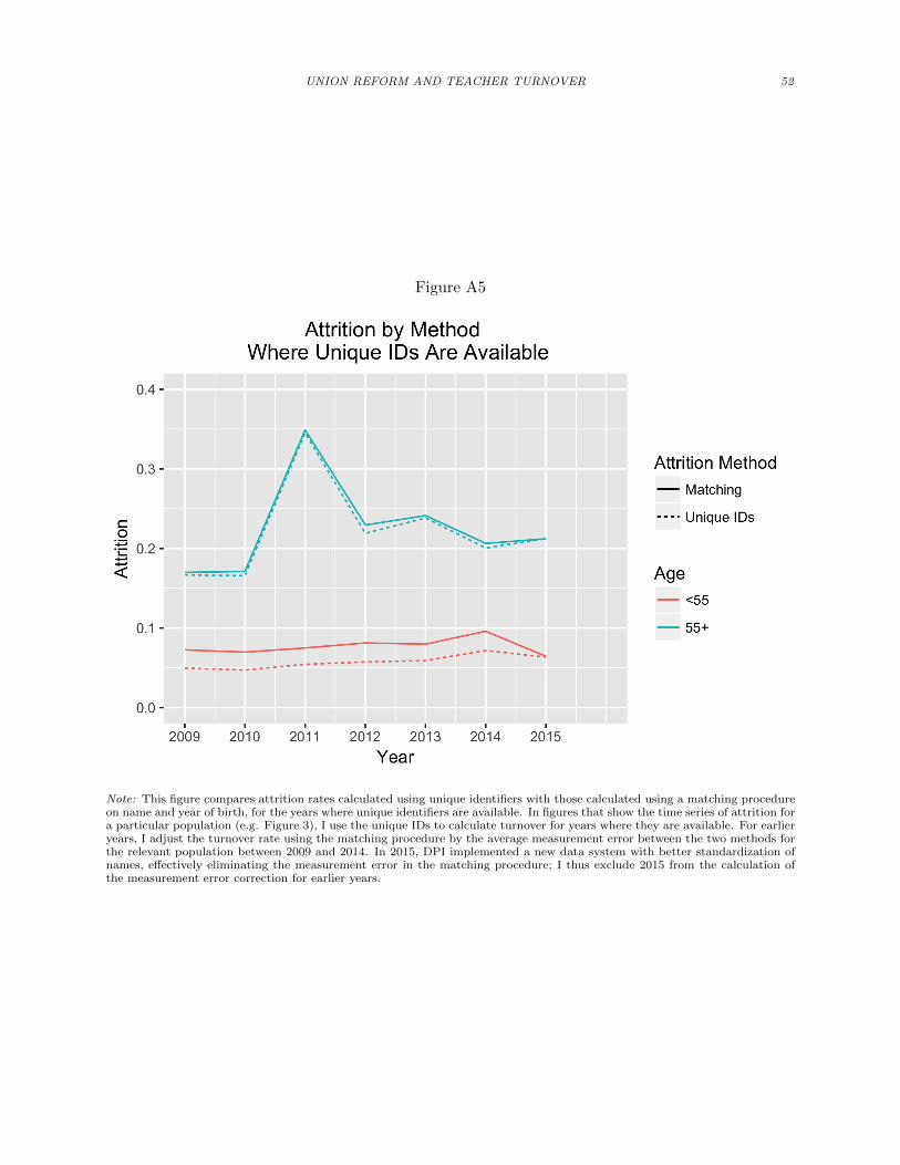
UNION REFORM AND TEACHER TURNOVER 52
Figure A5
Note: This figure compares attrition rates calculated using unique identifiers with those calculated using a matching procedureon name and year of birth, for the years where unique identifiers are available. In figures that show the time series of attrition fora particular population (e.g. Figure 3), I use the unique IDs to calculate turnover for years where they are available. For earlieryears, I adjust the turnover rate using the matching procedure by the average measurement error between the two methods forthe relevant population between 2009 and 2014. In 2015, DPI implemented a new data system with better standardization ofnames, effectively eliminating the measurement error in the matching procedure; I thus exclude 2015 from the calculation ofthe measurement error correction for earlier years.
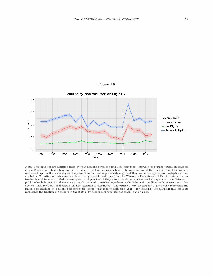
UNION REFORM AND TEACHER TURNOVER 53
Figure A6
Note: This figure shows attrition rates by year and the corresponding 95% confidence intervals for regular education teachersin the Wisconsin public school system. Teachers are classified as newly eligible for a pension if they are age 55, the minimumretirement age, in the relevant year; they are characterized as previously eligible if they are above age 55, and ineligible if theyare below 55. Attrition rates are calculated using the All Staff files from the Wisconsin Department of Public Instruction. Ateacher is said to have attrited between year t and year t+1 if they were a regular education teacher anywhere in the Wisconsinpublic schools in year t and were not a regular education teacher anywhere in the Wisconsin public schools in year t + 1. SeeSection III.A for additional details on how attrition is calculated. The attrition rate plotted for a given year represents thefraction of teachers who attrited following the school year ending with that year – for instance, the attrition rate for 2007represents the fraction of teachers in the 2006-2007 school year who did not teach in 2007-2008.