UNiON Wages aNd UNiON deCliNe: eVideNCe frOm the ...drdale/Publications/Labor Relations/Wage Gaps ILRR... · was amended in John DeKlewa and Sons, Inc., 281 NlrB (1987) to prevent

67

A

Industrial and Labor Relations Review, Vol. 60, No. 1 (October 2006). © by Cornell University. 0019-7939/00/6001 $01.00

UNiON Wages aNd UNiON deCliNe:

eVideNCe frOm the CONstrUCtiON iNdUstry

dale BelmaN and PaUla B. VOOs*

two well-documented empirical findings are that unionized employees typically receive substantially higher compensation than their non-union counterparts and that union representation in the United states has declined over time. some observers have hypothesized a causal link between these two phenomena: the achievement of a union wage premium, they argue, hastened union decline by inducing employers to adopt various union avoidance strategies. Using data from the Current Population survey and the Census Bureau’s Census of Construction, the authors test this hypothesis for the construction industry. even in estimations that allow for a lagged response and incorporate a variety of controls, they find no evidence that high union/nonunion wage ratios in construction in the 1970s or 1980s resulted in lower union membership in 2000.

*dale Belman is Professor of industrial relations and economics, michigan state University; associate direc-tor, sloan foundation trucking industry Program; and research associate, economic Policy institute. Paula B. Voos is Professor and Chair, labor studies and employ-ment relations department, school of management and labor relations, rutgers University. the authors thank stephen Woodbury, Jeffrey Keefe, richard Bloch, russell Ormiston, and Peter Berg for their comments on earlier drafts of this paper.

a data appendix with additional results, and copies of the computer programs used to generate the results presented in the paper, are available from the first author at school of labor & industrial relations, michigan state University, 401 s. Kedzie hall, east lansing, mi 48824-3285; [email protected].

1data are from the union membership and coverage website (hirsch and macpherson 2005).

merican labor unions have long em- phasized the direct economic represen-tation of their members through collective bargaining. through negotiations, they have managed to raise members’ wages and benefits substantially above the level paid to nonunion workers with the same skills and personal char-acteristics. Union-nonunion compensation differentials in the United states substantially exceed those found in Western europe today. this remains true despite the substantial decline in the percentage of the work force represented by unions in the private sector.

after peaking in the early 1950s at ap-proximately 35%, U.s. union membership in

the private sector went into gradual decline. Between 1979 and 2004, it fell from 21% to about 8%.1 many factors have contributed to the decline in union membership, including structural shifts in the locus of employment and a low rate of new union organizing (re-lated to the legal process of organizing in the United states, strenuous management opposition to unions, individualism on the part of workers, and other factors). some economists view high union/nonunion wage differentials as one factor contributing to both loss of existing union jobs and intense opposition by management to new union organization (freeman 1986; edwards and swaim 1986; linneman et al. 1990; Blanch-

68 iNdUstrial aNd laBOr relatiONs reVieW

flower and freeman 1992; hirsch and schum-acher 2001). according to these economists, the very success of U.s. unions in improving members’ compensation may have contrib-uted to their long-run failure to thrive.

the construction industry, an economi-cally important microcosm, provides a test of this general perspective on unions. thieblot (2001), for instance, has claimed that the long-run decline of union membership in construction is largely explained by high union/nonunion wage differentials. the logic is straightforward: in construction, compensation differentials exceeded pro-ductivity differentials, allowing nonunion firms to underbid organized firms; this led to a decline in union market share. Clearly, this could be an important factor explaining declining union membership in construction. Whether or not it was in fact a major driver of union decline is another matter—one we examine here.

deeper examination of the situation in construction may bear intellectual fruit, as it is an industry in which researchers are not con-fined to examining a single national trend. Construction has local and regional markets characterized by significant metropolitan and regional variation in both membership and wage differentials. thus, it is an industry in which it is possible to evaluate whether or not those local/regional markets with comparatively high union/nonunion dif-ferentials, other things equal, were areas in which unions experienced greater problems in maintaining market share in subsequent years. this within-industry research strat-egy controls for many things that may vary between industries. hence, we would argue that our research strategy has the potential to illuminate the general relationship between union/nonunion wage differentials and union decline.

the construction industry is also an excel-lent candidate for this research as it is more vulnerable to rapid de-unionization than many other domestic industries. although it is possible to de-certify unions, the common route to nonunion status in many industries has been the costly and gradual process of replacing organized facilities with nonunion facilities or the expansion of nonunion

corporations at the expense of organized corporations (or both). in contrast with the permanence of establishments in most industries, construction projects are brief endeavors. as a result, construction workers regularly move between projects and employ-ers. Construction firms can, with attention to legal restrictions, shift from being signatory on one project to operating as an open shop firm on the next if they are able to find quali-fied workers willing to work in an open shop. indeed, many of the larger firms operate as double-breasted enterprises, using their open shop subsidiary where possible and their signatory subsidiary where necessary.

the ability to de-unionize was historically limited by union control over construction training and the skilled labor force, pre-hire agreements, legal restrictions on operating with union and nonunion subsidiaries, and the ability of organized trades to strike if open shop contractors worked on a project. the Smith decision of the NlrB in 1971 allowed employers to pull out of pre-hire agreements unless construction unions could prove that they represented a majority of a contractor’s employees; the Kiewit decision (1977) sub-stantially increased the ability of construction firms to double-breast and then shift work to open shop subsidiaries (see allen 1994:433 for a discussion).2 following these decisions, in the period we study (1975–2000), it became much easier for a unionized contractor to become nonunion. hence unionization presumably became more sensitive to changes in economic factors such as union/nonunion wage differentials.

finally, the construction industry provides a particularly interesting test of the wage gap hypothesis because of unions’ central role in the training and certification of con-struction workers. the effects of wage gaps between groups of workers are mediated by systematic differences in the productivity of

2R. J. Smith Construction Co., 191 NlrB 693 (1971) was amended in John DeKlewa and Sons, Inc., 281 NlrB (1987) to prevent the employer from repudiating the agreement when it was in effect. the Kiewit decision went through two stages, Peter Kiewit and Sons, Inc., 206 NlrB 562 (1973), and the final decision 231 NlrB 76 (1977).

UNiON Wages aNd UNiON deCliNe 69

those groups. a group of more productive workers can obtain higher wages without suffering from unfavorable unit costs and their consequences. the construction trades have been deeply involved in worker training and certification through joint la-bor-management apprenticeship programs. these programs, which are regulated by the Bureau of apprenticeship training of the U.s. department of labor, require between three and five years of on-the-job and class-room training. Building trades unions and their signatory employers collectively invest in excess of $200 million annually in these training programs. much of the classroom and on-the-job training is provided by union trainers and members; unions play a key role in program oversight. in contrast, the open shop has faced serious problems in develop-ing effective training programs because it lacks the umbrella training organizations that exist in the organized sector, because individual employers are typically reluctant to provide general training, and because in-dividuals typically lack the funds needed to pursue training themselves. this weakness of training systems in the open shop has been extensively commented on by groups such as the Business round table.3

the difference between the union and nonunion sectors in training and skills has underlain differences in work organization: the union sector uses more highly trained and largely self-directed workers, while the open shop combines highly skilled key work-ers with larger numbers of supervised semi-skilled workers and helpers. the superior productivity of union workers may partially or entirely offset their higher wages.

Construction Union Membership and Wage Trends

as with union membership as a whole, there has been a large decline in the pro-portion of construction workers who belong to labor unions over the last three decades. Construction historically was a highly union-ized industry. allen (1994:425) reported that

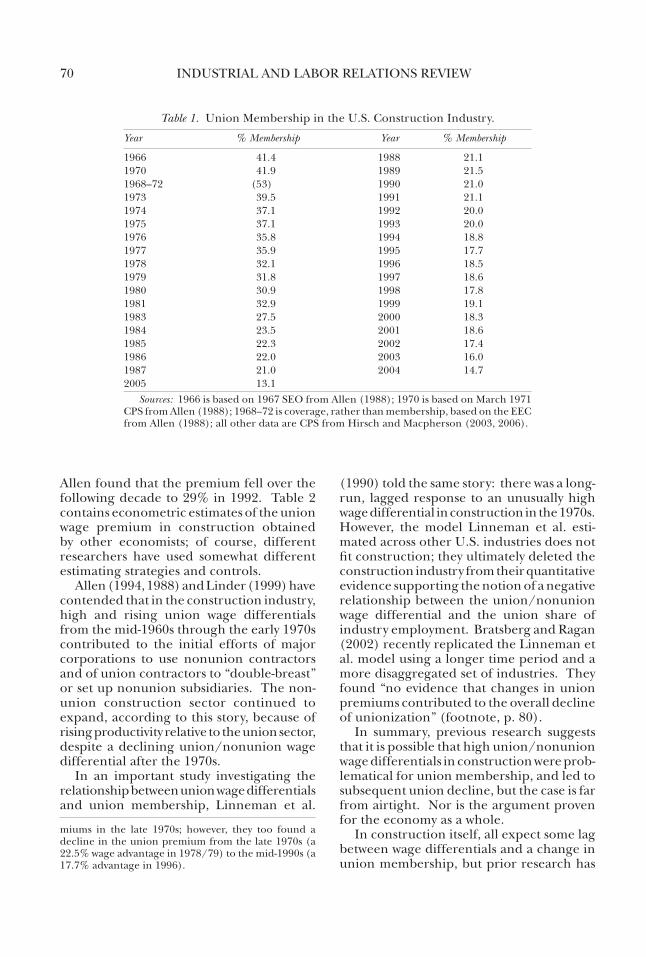
41.4% of all construction workers were union members in 1966. this number had fallen to 31.6% by 1979, and to 22.0% by 1989. according to the Current Population survey (CPs), union membership in construction stood at 13.1% in 2005—approximately double the unionization rate for the private sector as a whole. table 1 contains data de-tailing union membership in construction (coverage by collective agreements is only slightly higher).

historically, the union wage premium in construction was also relatively large, accord-ing to most extant econometric estimates. it is well known that although these estimates attempt to control for the observed character-istics of workers, they may not have controlled for all the relevant characteristics of construc-tion jobs, because standard data sets like the CPs do not contain information regarding, for example, whether a construction worker was employed in home-building or skyscraper or bridge projects. larger-scale construction projects typically have higher proportions of unionized workers, higher skill requirements, and more productive workers. in addition, the human capital of manual workers is in-completely measured in standard data sets because the measures of training, such as apprenticeship programs, are rudimentary. for those reasons, most standard estimates likely overstate the true union/nonunion differential in construction.

Nonetheless, econometric estimates of the union wage premium in construction were strikingly high in earlier years. allen (1994:430) estimated that the premium rose in the 1970s, peaking at 55.3% in 1977, up from 37.7% in 1967, but then declined in the 1980s as unions recognized that in order to recapture market share they would have to moderate the economic disadvantage facing union contractors. By 1983, allen (1994) found the premium stood at 44.3%, which is close to hirsch’s (1994) and linneman et al.’s (1990) findings of 39.6% and 41.6%, respectively, for that same year.4 however,

3see, for example, Training Problems in the Open Shop (Business round table 1990).

4according to linneman et al. (1990), the differen-tial peaked in 1974 at 51.2%, and declined to 40.4% by 1986. in contrast, Belman and Voos (2004) estimated substantially lower figures for construction wage pre-


allen found that the premium fell over the following decade to 29% in 1992. table 2 contains econometric estimates of the union wage premium in construction obtained by other economists; of course, different researchers have used somewhat different estimating strategies and controls.

allen (1994, 1988) and linder (1999) have contended that in the construction industry, high and rising union wage differentials from the mid-1960s through the early 1970s contributed to the initial efforts of major corporations to use nonunion contractors and of union contractors to “double-breast” or set up nonunion subsidiaries. the non-union construction sector continued to expand, according to this story, because of rising productivity relative to the union sector, despite a declining union/nonunion wage differential after the 1970s.

in an important study investigating the relationship between union wage differentials and union membership, linneman et al.

(1990) told the same story: there was a long-run, lagged response to an unusually high wage differential in construction in the 1970s. however, the model linneman et al. esti-mated across other U.s. industries does not fit construction; they ultimately deleted the construction industry from their quantitative evidence supporting the notion of a negative relationship between the union/nonunion wage differential and the union share of industry employment. Bratsberg and ragan (2002) recently replicated the linneman et al. model using a longer time period and a more disaggregated set of industries. they found “no evidence that changes in union premiums contributed to the overall decline of unionization” (footnote, p. 80).

in summary, previous research suggests that it is possible that high union/nonunion wage differentials in construction were prob-lematical for union membership, and led to subsequent union decline, but the case is far from airtight. Nor is the argument proven for the economy as a whole.

in construction itself, all expect some lag between wage differentials and a change in union membership, but prior research has

miums in the late 1970s; however, they too found a decline in the union premium from the late 1970s (a 22.5% wage advantage in 1978/79) to the mid-1990s (a 17.7% advantage in 1996).

Table 1. Union membership in the U.s. Construction industry.

Year % Membership Year % Membership

1966 41.4 1988 21.11970 41.9 1989 21.51968–72 (53) 1990 21.01973 39.5 1991 21.11974 37.1 1992 20.01975 37.1 1993 20.01976 35.8 1994 18.81977 35.9 1995 17.71978 32.1 1996 18.51979 31.8 1997 18.61980 30.9 1998 17.81981 32.9 1999 19.11983 27.5 2000 18.31984 23.5 2001 18.61985 22.3 2002 17.41986 22.0 2003 16.01987 21.0 2004 14.72005 13.1

Sources: 1966 is based on 1967 seO from allen (1988); 1970 is based on march 1971 CPs from allen (1988); 1968–72 is coverage, rather than membership, based on the eeC from allen (1988); all other data are CPs from hirsch and macpherson (2003, 2006).


had difficulty incorporating lags into models. for instance, linneman et al. (1990:19) noted that “attempts to incorporate lagged effects were not successful, due to the relatively short time span of the time series,” and when they modeled the change in density between 1973 and 1986 as a function of the change in the wage premium from 1973 to 1975, the coef-ficient was statistically insignificant. Problems incorporating lags may be one reason why research to date has failed to substantiate the “high wage differentials lead to union decline” story in construction.5 this is one

shortcoming of previous research that will be addressed in this study.

Before detailing our research design, we review essential background material on construction labor markets.

Construction Labor Markets

although some contractors bid for work

Table 2. Union/Nonunion Wage differentials in Construction.

Linneman Hirsch from Bratsberg & Year Allen (1988) et al. (1990) Allen (1994) Ragan (2002)a

1967 37.7%

1971 43.7%

1973 52.8 48.2% 45.91974 51.4 51.2 37.21975 54.8 46.9 48.61976 54.8 48.0 53.61977 55.3 46.6 46.71978 55.0 45.9 47.11979 41.5 34.8 37.41980 47.2 37.0 36.21981 38.8 36.2 35.11982 n/a 1983 44.3 41.6 39.6% 42.31984 42.5 41.0 43.21985 41.6 38.8 41.51986 40.4 38.3 41.21987 34.3 38.01988 31.8 35.91989 33.4 35.51990 28.8 30.51991 30.2 32.21992 29.0 32.01993 31.81994 29.71995 33.01996 28.91997 29.21998 27.91999 24.7

Note: the first three data columns in this table were published in allen (1994), who cited personal correspon-dence with hirsch as the source for column (3).

aCalculated from unpublished coefficients provided to us by the authors.

5Bratsberg and ragan (2002:73), in a series of “causal-ity tests,” did present one series of regressions with lags.

One regression had union density as the dependent variable, and the union wage premium lagged one and two years as independent variables, while controlling for density and imports with a similar lag structure. data were on 32 industries at the two-digit level in manufacturing and at the one-digit level outside manufacturing. the coefficient on the wage premium with the one-year lag was negative, and that on the wage premium with the two-year lag was positive.


on a national, and even an international, basis, construction labor markets remain primarily local or regional in nature. even when a national general contractor such as Bechtel, skanska, or Kellogg, Brown, and root is successful in obtaining a contract to build a power-plant or factory, that contrac-tor typically moves only a small group of managers and key workers to the project site. much of the work is subcontracted to local and regional firms with their own local labor force. even when the contractors hire directly, they usually use local sources, such as building trades unions or specialized labor recruiters, to obtain a skilled labor force for the project.6

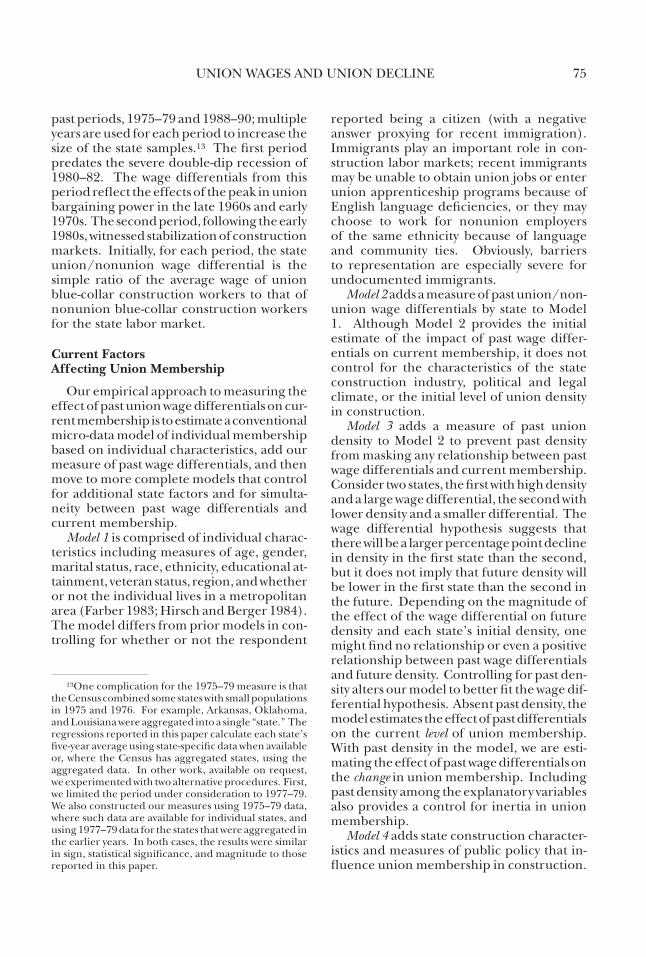
it should not be surprising that union-ization in construction varies substantially across states and metropolitan areas in the United states. although union member-ship in construction has declined in most local/regional markets, the decline has been much steeper in some markets than others. table 3 contains information on membership trends by state calculated from may Current Population surveys (CPs) for 1975–79 and from the CPs outgoing rotation files for 1988–90 and for 2000. Cross-state averages and the standard deviation of the state data are at the bottom of the table.

Prior to the double-dip recessions of 1980–82, blue-collar union density in construction averaged 35.9% across states, and ranged from 12.2% in North Carolina to 57.8% in michigan. By the late 1980s, average state density had declined to 24.6%.7 By the year 2000, mean density by state was 20.8% and ranged from 2.7% in North Carolina to 53.9% in Wisconsin. although the overall trend was one of decline, and there was a continued downward shift in density in many states over this period, the pattern varied greatly,

with union representation stabilizing or even increasing in some states between 1990 and 2000: in 2000, for example, density was above 50% in Wisconsin and illinois, and above 40% in three other states. even as average density fell from the 1970s to the present, the dispersion of density across states remained relatively stable.8

table 3 also provides data on the ratio of union to nonunion construction wages for 1975–79, 1988–90, and 2000.9 the cross-state average did not change greatly over the period under study. it was 1.38 in the 1970s, rose to 1.42 in the 1980s, and fell back to 1.32 in 2000. again, considerable cross-state varia-tion is evident in each period: in 2000 the ratio ranged from .94 in Vermont to 1.61 in West Virginia. in contrast with the stability of the dispersion of density over the period, the standard deviation of wage gaps rose steadily from 0.077 in the 1970s to 0.149 in 2000. state wage gaps became steadily less alike over the period.

the hypothesis that large wage differen-tials at one point in time will be associated with lower union density in the future is supported by the simple correlation of past differentials and current density. the correlation of the 1970s wage differential with year 2000 density is –.490 and is statistically significant in better than a 1% test (p = 0.03%).10 the correlation of the 1980s wage differential data and year 2000 density is –.351 and is close to signifi-cance in a 1% test (p = 1.16%). in contrast, the contemporaneous correlation of the year 2000 wage differential and density data, .355, is positive and also close to significance in a 1% test (p = 1.06%).11

6although some trades, such as boiler-makers, have national labor markets and other trades have some in-ter-regional movement of workers when there are local labor shortages, widespread inter-regional movement of construction workers is unusual, particularly outside the organized sector.

7the NBer dates the first recession of the early 1980s as starting in January 1980 and ending in July of that year, and the second recession as starting in July 1981 and ending in November 1982.

8the standard deviation of density moved over a narrow range of 0.111 (1970s) to 0.099 (1988–90) to 0.137 (2000).

9Both the density and earnings differentials are constructed using the CPs earnings weights data; the earnings differentials are not adjusted for worker characteristics.

10the likelihood of the null being true given the sample result, p, is 0.03%. We use p-values instead of the more conventional t-value because p-values can be interpreted without reference to tables. there is a direct correspondence between t- and p-values.

11as we will argue in our discussion of more complete models, the wage differential hypothesis may be better modeled as a relationship between past wage differentials


Table 3. Union density and Union/Nonunion Wage differentials: 1970s,1980s, and 2000.

Union Density Union/NonunionWage Differential

State 1975–1979 1988–1990 2000 1975–1979 1988–1990 2000

alabama 32.7% 25.6% 7.9% 1.57 1.48 1.24alaska 46.9% 26.0% 28.0% 1.33 1.37 1.14arizona 28.3% 11.6% 7.0% 1.40 1.32 1.35arkansas 24.9% 17.2% 9.9% 1.38 1.45 1.22California 40.7% 26.6% 29.3% 1.38 1.46 1.49Colorado 29.8% 18.2% 8.6% 1.40 1.46 1.19Connecticut 38.7% 28.2% 32.2% 1.21 1.27 1.24delaware 36.4% 31.3% 13.0% 1.36 1.34 1.40d.C. 41.8% 23.9% 24.6% 1.31 1.29 1.21florida 17.2% 11.4% 5.4% 1.44 1.47 1.30georgia 17.6% 15.4% 10.8% 1.58 1.56 1.36hawaii 47.5% 37.4% 40.5% 1.35 1.36 1.31idaho 30.3% 19.7% 9.8% 1.33 1.39 1.25illinois 52.3% 37.0% 53.7% 1.30 1.34 1.49indiana 54.4% 41.8% 38.0% 1.28 1.45 1.40iowa 39.9% 30.7% 19.9% 1.40 1.41 1.47Kansas 37.4% 24.4% 19.8% 1.40 1.47 1.55Kentucky 37.9% 31.5% 20.3% 1.32 1.37 1.56louisiana 25.4% 15.5% 14.9% 1.27 1.39 1.46maine 28.3% 21.1% 17.7% 1.30 1.47 1.36maryland 36.8% 26.4% 11.2% 1.39 1.28 1.25massachusetts 36.0% 28.2% 25.7% 1.33 1.25 1.28michigan 57.8% 45.2% 35.7% 1.33 1.43 1.43minnesota 41.0% 30.2% 38.9% 1.43 1.43 1.19mississippi 25.0% 13.4% 12.0% 1.47 1.40 0.98missouri 40.0% 32.0% 44.8% 1.46 1.51 1.44montana 32.4% 26.6% 16.1% 1.45 1.56 1.12Nebraska 37.4% 19.0% 9.1% 1.41 1.54 1.39Nevada 31.1% 21.2% 28.4% 1.45 1.40 1.50New hampshire 27.6% 16.0% 27.7% 1.31 1.27 1.36New Jersey 51.4% 39.9% 40.8% 1.23 1.26 1.40New mexico 27.4% 15.1% 8.0% 1.35 1.46 1.24New york 51.1% 39.6% 39.1% 1.25 1.36 1.40North Carolina 12.2% 7.8% 2.7% 1.47 1.46 1.13North dakota 37.0% 18.5% 13.5% 1.40 1.75 1.27Ohio 54.9% 40.4% 35.3% 1.30 1.39 1.50Oklahoma 27.3% 18.4% 2.9% 1.36 1.50 1.46Oregon 39.7% 32.5% 32.4% 1.36 1.36 1.49Pennsylvania 53.8% 36.2% 29.5% 1.30 1.30 1.34rhode island 30.0% 21.1% 30.5% 1.33 1.26 1.30south Carolina 14.4% 8.0% 3.7% 1.48 1.37 1.06south dakota 35.6% 13.2% 8.5% 1.39 1.59 1.23tennessee 34.8% 20.4% 15.6% 1.35 1.47 1.05texas 20.0% 11.3% 4.2% 1.47 1.52 1.30Utah 28.4% 14.2% 10.4% 1.45 1.49 1.22Vermont 30.3% 16.1% 15.8% 1.32 1.25 0.93Virginia 32.6% 16.5% 2.9% 1.39 1.37 1.38Washington 51.2% 39.0% 23.3% 1.42 1.40 1.37West Virginia 40.5% 38.3% 19.7% 1.45 1.47 1.61Wisconsin 53.6% 33.8% 53.9% 1.34 1.42 1.35Wyoming 29.2% 21.4% 6.9% 1.39 1.56 1.24

average 35.9% 24.6% 20.8% 1.375 1.416 1.318std. dev. 11.1% 9.9% 13.7% 0.077 0.102 0.149

Notes: data are from the 1975–79 may CPs, the 1988–90 CPs Org files, or the 2000 CPs Org files. earnings weights are used in calculating averages. Wage differentials are not adjusted for worker characteristics.


Considering all three correlations, there is some, but far from conclusive, support for the wage differential hypothesis. We now turn to more complete models that control for a range of factors affecting density.

Empirical Strategy

Our strategy is to estimate a conventional model of the contemporaneous individual characteristics influencing the likelihood of a blue-collar construction employee be-longing to a labor organization, test for the added effect of past state union/nonunion wage differentials on that likelihood, and then introduce other controls for charac-teristics of state construction to determine how these affect the relationship between wage differentials and union membership. We estimate the membership equation with individual data from the 2000 CPs Outgo-ing rotation file in a probit equation. Our model takes the form

(1) MeMbershipij = F(gwgWagegapjt + b'Xij + g'Zj' + eij + hj,

where MeMbershipij is a 0/1 indicator of union membership; gwg is the coefficient on the state wage gap in 1975–79 or 1988–90; Wagegapjt is the union/nonunion wage gap in construction in 1975–79 or 1988–90; b is the vector of individual coefficients; X is the vector of individual characteristics; g is the vector of coefficients for state charac-teristics other than the wage gap; Z is the vector of state characteristics; eij is the error for individual i in state j; hj is the common error for all individuals in state j; i indexes individuals; j indexes states; and t indexes the time period for the wage gap, 1975–79 or 1988–90. gwg is the coefficient of interest,

the measure of the impact of past union/nonunion state wage gaps in construction on current membership. Operationalizing this model requires defining construction labor markets, developing measures of the union/nonunion wage differentials, and determining the individual characteristics and state factors that might reasonably be expected to influence union membership. these will be discussed in turn.

The Definition of Labor Markets

Construction labor markets are centered around urban areas, but draw their labor from an area considerably larger than the metropolitan statistical areas used by the Census. some labor markets cross state boundaries; some are smaller than states; and some approximate the state in which the metropolitan area is located. however, even though the fit between labor markets and states is imperfect, states are used in this study to proxy labor markets. that is done because prior to 1983, the number of observations on construction workers in many cities is too small to provide reliable estimates of unionization even when several years of data are combined.12 an advantage of using states is that detailed information on the construction industry by state is available from the Census of Construction, prepared by the Bureau of the Census. the Census of Construction is issued at five-year intervals; the 1977, 1987, and 1997 data sets are used in this study.

Measures of Past Wage Differentials

although our model takes individual union membership as its dependent variable, data on past wage differentials are necessarily a la-bor market average. We use averages from two

and changes in density, which allows for differences in density between states at the beginning of the period under study, than as a relationship between gaps and levels, which does not. the correlation of the 1970s state wage gap with the change in density from the 1970s to 2000 is –.0999, correctly signed but far from statistically significant (p = 48.6%). the correlation of the 1980s wage gap with the 1980s–2000 change in density is –.266 and, in contrast with the 1970s result, is weakly significant (with a p-value of 5.89%).

12We are particularly interested in the effect of wage gaps prior to the 1980–82 double-dip recession. this recession, the worst experienced by american workers since the great depression, was instrumental in the restructuring of construction labor markets. National membership in construction unions declined by 6% between 1979 and 1985, and there was a large effect on union wages in the industry. to avoid starting in media res, we require measures predating this recession.


past periods, 1975–79 and 1988–90; multiple years are used for each period to increase the size of the state samples.13 the first period predates the severe double-dip recession of 1980–82. the wage differentials from this period reflect the effects of the peak in union bargaining power in the late 1960s and early 1970s. the second period, following the early 1980s, witnessed stabilization of construction markets. initially, for each period, the state union/nonunion wage differential is the simple ratio of the average wage of union blue-collar construction workers to that of nonunion blue-collar construction workers for the state labor market.

Current Factors Affecting Union Membership

Our empirical approach to measuring the effect of past union wage differentials on cur-rent membership is to estimate a conventional micro-data model of individual membership based on individual characteristics, add our measure of past wage differentials, and then move to more complete models that control for additional state factors and for simulta-neity between past wage differentials and current membership.

Model 1 is comprised of individual charac-teristics including measures of age, gender, marital status, race, ethnicity, educational at-tainment, veteran status, region, and whether or not the individual lives in a metropolitan area (farber 1983; hirsch and Berger 1984). the model differs from prior models in con-trolling for whether or not the respondent

reported being a citizen (with a negative answer proxying for recent immigration). immigrants play an important role in con-struction labor markets; recent immigrants may be unable to obtain union jobs or enter union apprenticeship programs because of english language deficiencies, or they may choose to work for nonunion employers of the same ethnicity because of language and community ties. Obviously, barriers to representation are especially severe for undocumented immigrants.

Model 2 adds a measure of past union/non-union wage differentials by state to model 1. although model 2 provides the initial estimate of the impact of past wage differ-entials on current membership, it does not control for the characteristics of the state construction industry, political and legal climate, or the initial level of union density in construction.

Model 3 adds a measure of past union density to model 2 to prevent past density from masking any relationship between past wage differentials and current membership. Consider two states, the first with high density and a large wage differential, the second with lower density and a smaller differential. the wage differential hypothesis suggests that there will be a larger percentage point decline in density in the first state than the second, but it does not imply that future density will be lower in the first state than the second in the future. depending on the magnitude of the effect of the wage differential on future density and each state’s initial density, one might find no relationship or even a positive relationship between past wage differentials and future density. Controlling for past den-sity alters our model to better fit the wage dif-ferential hypothesis. absent past density, the model estimates the effect of past differentials on the current level of union membership. With past density in the model, we are esti-mating the effect of past wage differentials on the change in union membership. including past density among the explanatory variables also provides a control for inertia in union membership.

Model 4 adds state construction character-istics and measures of public policy that in-fluence union membership in construction.

13One complication for the 1975–79 measure is that the Census combined some states with small populations in 1975 and 1976. for example, arkansas, Oklahoma, and louisiana were aggregated into a single “state.” the regressions reported in this paper calculate each state’s five-year average using state-specific data when available or, where the Census has aggregated states, using the aggregated data. in other work, available on request, we experimented with two alternative procedures. first, we limited the period under consideration to 1977–79. We also constructed our measures using 1975–79 data, where such data are available for individual states, and using 1977–79 data for the states that were aggregated in the earlier years. in both cases, the results were similar in sign, statistical significance, and magnitude to those reported in this paper.


Construction union membership is typically higher in the segments of construction that require greater work force skills. We hypoth-esize that if an individual construction worker lives in a state with a greater proportion of residential construction where fewer skills are required, that person will have a lower prob-ability of being a union member, other things equal; the probability will be higher if a larger proportion of the value of construction is in non-building construction (highway, public works, and industrial). the model also adds the rate of growth of the construction market in a given state as a control variable.14

the state’s legal environment and public expenditures on construction are also in-cluded in model 4. One variable is whether or not the state has a state prevailing wage law; such laws are favorable to unions, as they remove direct labor costs from competition and provide labor cost savings for the use of apprentices from registered programs.

Public expenditures on construction may also affect union membership. almost all federal expenditures on construction are covered by the davis-Bacon act, and we would expect this to provide an advantage to organized contractors. states in which the federal government accounts for a larger proportion of construction expenditures should have higher membership.

a final control variable in model 4 is the proportion of construction expenditures ac-counted for by state and local government. most states require that public construction contracts go to the lowest qualified bidders. although there are arguments about whether or not low bid systems result in lower final costs or better projects than alternative bidding systems, the low bid system favors contractors with lower and more flexible labor costs, and these tend to be nonunion contractors. if public contracting procedures favor nonunion firms, states in which public contracting comprises a larger proportion of

total construction expenditures should have lower union membership. this leads us to hy-pothesize that the coefficient on this control variable will be negative, although we recog-nize other arguments could be made about the expected sign of this coefficient.15

Model 5 adds a measure of blue-collar union density outside of construction to our basic model. We think of this control vari-able as a proxy for all the additional factors (right-to-work laws, political power of the state labor movement, and so on) that might influence union membership generally in a given state.

a more complete approach to the issue of “unobserved state factors” is our next subject of discussion.

The Error Structure

finally, the logic of a model in which both individual and state factors are included among the explanatory variables strongly sug-gests that the error may not be independently and identically distributed. if state charac-teristics affect individual union membership outcomes, the presence of omitted state characteristics or the mis-measure of state data will result in a state error component.

different assumptions about the char-acteristics of the state error term require different approaches to estimation. in our initial estimates we assume that the state er-ror terms are orthogonal to the explanatory variables and estimate the model using an approach that, in a linear model, would be characterized as a random effects model.16 in general, the correction results in larger standard errors and lower t-values for the state

14We measure the importance of residential and non-building construction and growth of construction with data from the 1997 Census of Construction; the growth variable measures growth in the value of construction from 1994 to 1997.

15states with a larger proportion of construction funded by the public sector may provide favorable con-ditions for unions and union membership if unions are able to use their political influence to capture a larger share of public construction funds. this logic is less compelling in recent times, as the increasing political influence of open shop contractors associations such as the associated Builders and Contractors may counterbal-ance union influence.

16We use the cluster option provided in stata for probit models (reference K-Q stata 9, pp. 469–83 http://www.stata.com/support/faqs/stat/robust_ref.html) to correct for the state component.


characteristics variables but has little effect on the standard errors of the variables measured at the individual level. in a later section of this paper, we discuss additional estimates that relax this assumption, allow the state error term to be correlated with prior values of the wage gap and construction union density, and correct for this potential simultaneity using the method developed by rivers and Vuong (see Wooldridge 2002:472–77).

Econometric Evidence

results of our estimates are contained in table 4 (the effect of the 1970s wage differen-tials on year 2000 membership) and table 5 (the effect of 1980s wage differentials on year 2000 membership). all models are estimated allowing for a state error component.

Estimates Using Differentials from 1975–1979

Our base model of union membership in construction, model 1, is presented in the first column of table 4. the value in the table is the derivative of the likelihood function with respect to the variable and may be interpreted as the percentage change in the likelihood of observing a union member for a one unit change in the explanatory variable. the value in parentheses is the t-statistic for the coef-ficient. the set of independent variables in model 1 is comprised entirely of individual characteristics: education, age, gender, race, veteran status, citizenship, occupation, re-gion, and metropolitan status. as this is a model of blue-collar union membership, occupational indicators are limited to opera-tive and laborer, with precision production (skilled trades) as the base group.17

the results are consistent with past re-search on union membership. the effects of age, education, metropolitan status, region, and occupation are conventional; education, for instance, has a nonlinear relationship with membership. age has a positive convex relationship with membership: older work-

ers were more likely to be members, but the rate of increase declined with age. Women were neither more nor less likely than men to be union members; the same holds for veterans versus non-veterans. the results for race and ethnicity are more interesting. african-americans were 3.5% more likely to be union members than otherwise similar white construction workers. although the magnitude of the effect is not large, it con-tradicts the notion of racial discrimination by unions in the building trades. there was no statistically meaningful relationship between other racial/ethnic categories (for example, hispanic ethnicity) and union membership.

Our inclusion of indicators for both hispanic ethnicity and the respondents’ citizenship departs from the approach to ethnicity taken by prior research. We find a strong positive relationship between citizen-ship and membership. a non-citizen was 8.0% less likely to be a union member than an otherwise similar employee who was a citizen; in the only other study investigating this issue of which we are aware, Bratsberg, ragan, and Nasir (2002) found a citizenship effect of about the same magnitude. With this control, hispanics were no more or less likely than other workers to be union members. (in other regressions, available on request, without the citizenship control, the coeffi-cient on hispanic is negative and statistically significant.) apparently, the variable most closely tied to lack of unionization for some hispanics is recency of immigration, which is linked to lack of citizenship and, possibly, undocumented status.

taken together, these results are consistent with prior research on union membership.18 as the coefficients on these variables change very modestly in more complete specifica-

17all models using state average data from 1975–79 are estimated with 7,236 observations; the pseudo r2 for model 1 is 13.47%.

18the effects of metropolitan status, region, and occupation are those commonly found. Construction workers residing in metropolitan areas were more likely to be union members; those residing in the south were considerably less likely to be union members. skill was also positively associated with union membership. Operatives such as heavy equipment operators were no more or less likely to be members than craft workers; but laborers were less likely to be members.


tions, we will omit those specifications from further discussion.

model 2, in the second column, adds the 1970s state wage differential variable to model 1. the wage gap variable is negative, but far from statistically significant. although this suggests that there is no relationship between past wage gaps and current membership, once one controls for personal attributes of work-ers, it is possible that the true relationship is

being “masked” by the failure to control for initial union density.19 We explore this pos-

Table 4. the effect of 1970s Union Wage gaps on year 2000 Union density in Construction. (marginal effects—the derivative of the probit function—are reported in place of coefficients)

Add Add Human Add Add State Non- Capital 1970s 1970s Characteristics Construction Variable Model Wage Gap Density & Policies Density

average Wage gap, 1975–79 –0.0557 0.1076 0.0004 0.0553 (–0.40) (1.41) (0.00) (0.62)average Union density, 1975–79 0.7916 0.6403 0.4344 (8.52) (5.40) (3.66)Proportion residential Constructiona –0.2174 –0.1994 (–1.05) (–1.18)Proportion Non-Building Constructiona –0.1417 –0.1216 (–0.67) (–0.69)growth of state Construction, 1994–97a 0.0193 0.0963 (0.17) (0.92)federal Constructiona 0.2183 0.3271 (0.38) (0.64)state and local Constructiona –0.7827 –0.6256 (–1.91) (–1.75)state had a Prevailing Wage law in 2000 0.0569 0.0511 (2.67) (2.44)Non-Construction Blue-Collar density (2000) 0.4877 (2.96)some high school 0.0251 0.0250 0.0217 0.0221 0.0211 (1.19) (1.17) (1.01) (1.02) (0.98)high school degree 0.1084 0.1082 0.1025 0.1031 0.1028 (6.74) (6.73) (6.15) (6.24) (6.34)some College 0.1430 0.1423 0.1380 0.1410 0.1406 (6.06) (6.04) (5.70) (5.71) (5.83)associate’s or trade degree 0.1736 0.1728 0.1724 0.1758 0.1810 (5.35) (5.38) (5.29) (5.49) (5.70)Bachelor’s degree 0.0755 0.0754 0.0697 0.0729 0.0708 (2.35) (2.35) (2.12) (2.22) (2.12)Post-graduate degree –0.1517 –0.1519 –0.1474 –0.1441 –0.1407 (–3.72) (–3.72) (–3.67) (–3.40) (–3.25)age 0.0179 0.0179 0.0178 0.0177 0.0175 (6.93) (6.96) (6.90) (6.88) (6.85)age2 –0.0002 –0.0002 –0.0002 –0.0002 –0.0002 (–5.48) (–5.49) (–5.48) (–5.42) (–5.36)

Continued

19One referee suggested an estimating strategy based on an idea similar to model 3: a first difference equation using aggregated (state-level) data. this would test the hypothesis that the change in union density in a state is negatively related to the change in the wage gap. We grouped the data by states and then, estimating models similar to models 2–5 omitting the past density variable, regressed the change in density on the change in the


Table 4. Continued.


female –0.0132 –0.0128 –0.0101 –0.0089 –0.0099 (–0.45) (–0.43) (–0.34) (–0.30) (–0.33)married 0.0505 0.0507 0.0470 0.0472 0.0480 (5.62) (5.62) (5.33) (5.56) (5.73)Black 0.0357 0.0353 0.0294 0.0309 0.0303 (1.38) (1.37) (1.28) (1.34) (1.32)Other race 0.0098 0.0076 –0.0117 –0.0078 –0.0061 (0.19) (0.14) (–0.28) (–0.18) (–0.14)hispanic –0.0034 –0.0034 0.0027 –0.0047 0.0033 (–0.11) (–0.11) (0.11) (–0.19) (0.13)Veteran –0.0009 –0.0008 0.0066 0.0078 0.0069 (–0.07) (–0.06) (0.52) (0.62) (0.56)Non-Citizen –0.0802 –0.0809 –0.0863 –0.0846 –0.0835 (–3.32) (–3.36) (–3.64) (–3.48) (–3.42)lives in metropolitan area 0.0845 0.0847 0.0626 0.0573 0.0591 (4.96) (5.05) (3.92) (4.20) (4.24)lives in City of 1 million or more 0.0509 0.0504 0.0189 0.0144 0.0165 (2.88) (2.93) (1.24) (1.09) (1.29)lives in Northeast 0.0816 0.0788 0.1044 0.1014 0.0673 (2.41) (2.33) (3.96) (2.35) (1.65)lives in midwest 0.1173 0.1227 0.0739 0.0964 0.0596 (2.69) (2.51) (2.83) (4.07) (2.07)lives in south –0.1382 –0.1377 –0.0031 –0.0367 –0.0512 (–3.80) (–3.73) (–0.10) (–1.22) (–2.06)Operative –0.0378 –0.0372 –0.0347 –0.0362 –0.0374 (–1.05) (–1.03) (–0.98) (–1.01) (–1.08)laborer –0.0319 –0.0314 –0.0355 –0.0359 –0.0366 (–2.40) (–2.39) (–2.61) (–2.61) (–2.71)

Obs. P 0.2224 0.2224 0.2224 0.2224 0.2224Pred. P 0.1833 0.1833 0.1770 0.1764 0.1749ln likelihood –3317.81 –3317.19 –3223.64 –3206.32 –3195.25Pseudo r2 0.1347 0.1348 0.1592 0.1638 0.1666

aas a proportion of the 1997 value of construction.Parenthesized numbers are t-statistics. all models are estimated with 7,236 observations. marginal effects and

the predicted probabilities are computed at the means of the explanatory variables.

state wage gap and our other variables. estimates of the effect of the change in the wage gap were mixed in sign but far from statistically significant in all estimates. estimates in which the change in density was regressed on past wage gaps produced similar results. the esti-mates are available on request. although the results

sibility by adding a measure of 1970s union density by state in the third column of table 4 (model 3). as expected, the effect of past union density is large, positive, and statisti- from these alternative approaches were consistent with

our estimates, the small number of observations and degrees of freedom available in the state aggregated models make these tests less powerful than the one we adopt here.

20a ten percentage point difference between state density in the 1970s is estimated to have been associ-ated with a 7.98% increase in the likelihood of being a union member in 2000.

cally robust.20 however, with this addition, the effect of the wage gap becomes, counter to


expectations, positive. (although it is weakly statistically significant in a one-tailed test, not too much should be made of this result, as estimates from more complete models sug-gest that the wage gap measure is proxying for the effects of other state factors.)

the fourth column of table 4 (model 4) adds controls for state construction charac-teristics and for policy-related factors. the effect of the wage gap remains positive, but it now becomes statistically insignificant. the coefficients on the state prevailing wage law variable and the state and local funding for construction measure are statistically mean-ingful. as expected, the presence of a state prevailing wage law resulted in increased union membership; workers in states with such laws were 5.7% more likely to be mem-bers than similar workers in other states. in contrast, a higher proportion of state and local government funding of construction reduced the likelihood of union member-ship. a ten percentage point increase in state and local governments’ proportion of construction expenditures reduces the likelihood of union membership by 0.8%. this is consistent with the view that a low bid system works to the disadvantage of signatory construction firms.

On the other hand, there is little evidence that the distribution of the types of construc-tion or the recent growth of construction affected union membership. Neither the proportion of residential or non-building construction nor the growth rate is statistically significant. the measure of the proportion of construction funded by the federal govern-ment is also not statistically significant.

addition of a measure of non-construction blue-collar density by state to the model, model 5 of table 4, does not greatly affect our estimates. there is no meaningful change in the wage differential variable. as in most prior models, it falls well short of statistical significance. the added control variable, non-construction union density in the state, is positive, large in magnitude, and statistically significant. a 1% increase in non-construction density is estimated to have been associated with a .5% increase in construction density. the impact of prior construction density is about a third smaller

in magnitude but remains strongly statisti-cally significant.

in sum, the evidence does not support the hypothesis that high union/nonunion wage differentials in the 1970s resulted in lower union membership in the year 2000. Once one controls for the other factors influenc-ing union membership, the simple negative correlation between prior wage differentials and later union membership reverses in sign and is typically not statistically significant.

Estimates Using Differentials from 1988–1990

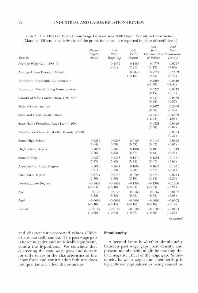
Parallel estimates using the 1988–90 wage differentials are presented in table 5; all of the models are estimated with 7,329 obser-vations. the human capital estimates in the first column are very similar to those of model 1 in table 4.21 the results in the sec-ond column are from an estimation (model 2) that adds the 1988–90 wage differential to the human capital model. a ten percent-age point increase in the wage differential between states is estimated to have increased union membership by 2.5%, a statistically significant result at odds with the hypothesis. adding a measure of construction density by state (model 3, in column 3) reduces the estimated effect of the 1980s wage differen-tial. a ten percentage point increase in the wage differential is now estimated to have increased membership by about 1.5%. Past density continues to have a large effect on current density.

as in the estimates with 1970s wage dif-ferentials and density, the positive effect of the wage differential loses its statistical signifi-cance once we control for other state factors. model 4 adds controls for the distribution of types of construction, the growth of con-struction, prevailing wage laws, and the role

21the reason there were more observations for the table 5 estimates than for the table 4 estimates is that data from states excluded from the table 4 estimates (because the estimates of the 1975–79 differential averages had fewer than thirty observations on union members) were included in the table 5 estimates (because the 1988–90 differentials had at least thirty union observations). the change in sample size had very small effects on coefficient estimates.


of the public sector in funding construction. results on these control variables are similar to the results reported in table 4, with minor exceptions.22 With the addition of the state characteristics, the wage differential variable is no longer statistically significant. the ad-dition of a control for current blue-collar density outside of the construction industry (model 5) does not affect these results. the wage differential remains non-significant.23 Our bottom line is that these results do not support the proposition that high union/nonunion wage differentials in the late 1980s had negative consequences ten years later for union membership in construction.

Allowing for Productivity and Simultaneity

to this point, the estimates have not sup-ported the wage differential hypothesis. the derivative of the wage differential variable is almost never negative. it is typically not sta-tistically significant. it is never negative and statistically significant; it is occasionally posi-tive and significant, contra the hypothesis.

although these estimates make a prima facie case against the wage gap hypothesis, some early reviewers of our research speculated that the true negative effect of the wage gap might be masked by systematic differences between union and nonunion productivity by state or by simultaneity between past wage gaps, past density, and current union mem-bership. the next section explores these issues in turn.

Correcting for Productivity Differences

as suggested in our prior discussion, wage gaps that are balanced by parallel differences

in productivity would not be expected to be associated with declining union density. Our failure to find a wage gap/membership rela-tionship may be due not to the lack of such a relationship, but rather to our failure to allow for systematic differences in productivity be-tween union and nonunion workers by state. We examine this possibility by estimating a past state union/nonunion wage gap model and substituting the predicted values from that model in our membership equation. in essence, we substitute a measure of the past wage gap that is corrected for differences in the characteristics of the state construc-tion labor force and industry for the actual measure used in our first set of estimates. We also estimate a model of past union density by state and include the predictions of those models where appropriate.24

the estimates of the effects of past wage gaps and past density obtained with charac-teristic-adjusted estimates are qualitatively similar to those obtained with the actual estimates (table 6, top panel). estimates of past wage gap effects using 1970s data are positive, but not statistically significant. as before, the effect of past density is positive and statistically significant in better than a 1% test; the impact is, however, somewhat smaller in magnitude than that obtained from the actual values. With the 1980s estimates of the wage gap, results in the various models estimated with the actual values (table 5)

22the proportion of construction expenditures accounted for by residential construction has a large, statistically significant negative effect on membership; a state with a ten percentage point higher proportion of construction expenditures in residential would have had 2.3% lower union membership in construction. this is consistent with the view that the lower skill levels required in residential construction increase the competitiveness of open shop construction firms.

23One referee correctly pointed out that the wage differential is measured with error, which biases the coefficient toward zero.

24Both of the “first stage models” include state aver-ages for age, education, race, ethnicity, marital status, veteran status, region, metropolitan status, total con-struction employment, the net value of construction, the percentage of construction comprised of residential work and the percentage non-building, whether the state had a prevailing wage law at that time, and the percentage of construction employment in small firms. the past wage differential equation included a measure of the union/nonunion blue-collar wage differential of non-construction employees at that time. the density equation included a measure of blue-collar union density among employees outside of the construction industry at that time. the first-stage models estimated with 51 observations and the estimates of past wage gaps and density are merged into our prior data set by state. the same number of observations is used for the membership equations as for the counterpart equations that do not allow for simultaneity.


and characteristic-corrected values (table 6) are markedly similar. the past wage gap is never negative and statistically significant, contra the hypothesis. We conclude that correcting the state wage gaps and density for differences in the characteristics of the labor force and construction industry does not qualitatively affect the estimates.

Simultaneity

a second issue is whether simultaneity between past wage gaps, past density, and present membership might be masking the true negative effect of the wage gap. simul-taneity between wages and membership is typically conceptualized as being caused by

Table 5. the effect of 1980s Union Wage gaps on year 2000 Union density in Construction. (marginal effects—the derivative of the probit function—are reported in place of coefficients)


average Wage gap, 1988–90 0.2457 0.1483 0.0778 0.0747 (2.11) (2.91) (1.12) (1.06)average Union density, 1988–90 0.8040 0.7774 0.7503 (13.16) (9.93) (6.73)Proportion residential Constructiona –0.2288 –0.2310 (–1.39) (–1.42)Proportion Non-Building Constructiona 0.0225 0.0212 (0.15) (0.14)growth of state Construction, 1994–97a 0.0373 0.0439 (0.48) (0.57)federal Constructiona 0.2075 0.2069 (0.56) (0.56)state and local Constructiona –0.6542 –0.6489 (–2.04) (–2.03)state had a Prevailing Wage law in 2000 0.0321 0.0325 (2.08) (2.09)Non-Construction Blue-Collar density (2000) 0.0504 (0.32)some high school 0.0212 0.0203 0.0125 0.0143 0.0143 (1.04) (0.99) (0.59) (0.67) (0.67)high school degree 0.1074 0.1056 0.1001 0.1019 0.1019 (6.76) (6.55) (6.37) (6.43) (6.43)some College 0.1379 0.1358 0.1319 0.1351 0.1351 (5.97) (5.83) (5.74) (5.67) (5.68)associate’s or trade degree 0.1656 0.1644 0.1603 0.1645 0.1651 (5.21) (5.13) (5.20) (5.37) (5.41)Bachelor’s degree 0.0757 0.0746 0.0723 0.0745 0.0744 (2.36) (2.30) (2.19) (2.24) (2.23)Post-graduate degree –0.1484 –0.1468 –0.1388 –0.1368 –0.1366 (–3.64) (–3.48) (–3.34) (–3.23) (–3.22)age 0.0173 0.0176 0.0168 0.0167 0.0167 (6.82) (6.88) (6.53) (6.58) (6.58)age2 –0.0002 –0.0002 –0.0002 –0.0002 –0.0002 (–5.40) (–5.45) (–5.16) (–5.16) (–5.16)female –0.0187 –0.0182 –0.0108 –0.0102 –0.0104 (–0.65) (–0.64) (–0.37) (–0.35) (–0.36)

Continued


unobserved individual factors common to (a) the wage level and the union employer’s decision to hire a particular individual, or (b) the wage level and the decision of a person to become a union member, or (c) the two together (robinson 1989; hirsch 2004). here, the common unobserved vari-able cannot be individual, both because the measure of the past wage differential is a state aggregate and because it predates our

2000 CPs data on individuals by 10 to 20 years. any simultaneity must then be due to an omitted time-invariant state factor (hj in equation 1) that affected both past wage differentials and variables included in the current membership equation.25

Table 5. Continued.


married 0.0474 0.0459 0.0463 0.0459 0.0459 (5.36) (5.19) (5.56) (5.66) (5.70)Black 0.0566 0.0646 0.0369 0.0399 0.0397 (1.85) (1.96) (1.60) (1.64) (1.64)Other race 0.0157 0.0174 –0.0323 –0.0282 –0.0274 (0.29) (0.31) (–0.97) (–0.82) (–0.77)hispanic –0.0026 –0.0014 0.0112 0.0077 0.0081 (–0.09) (–0.05) (0.47) (0.31) (0.32)Veteran 0.0018 0.0023 0.0078 0.0090 0.0089 (0.14) (0.18) (0.63) (0.73) (0.72)Non-Citizen –0.0812 –0.0817 –0.0896 –0.0877 –0.0876 (–3.43) (–3.39) (–4.03) (–3.83) (–3.82)lives in metropolitan area 0.0835 0.0828 0.0692 0.0661 0.0660 (4.88) (4.80) (4.95) (5.05) (5.00)lives in City of 1 million or more 0.0480 0.0462 0.0165 0.0169 0.0171 (2.88) (2.66) (1.35) (1.42) (1.45)lives in Northeast 0.0804 0.0916 0.0366 0.0408 0.0386 (2.38) (2.98) (1.79) (1.45) (1.31)lives in midwest 0.1275 0.0916 0.0156 0.0273 0.0260 (2.96) (2.00) (0.81) (1.27) (1.14)lives in south –0.1416 –0.1413 –0.0430 –0.0584 –0.0595 (–3.96) (–4.56) (–2.10) (–2.54) (–2.67)Operative –0.0334 –0.0311 –0.0284 –0.0309 –0.0310 (–0.95) (–0.88) (–0.85) (–0.93) (–0.93)laborer –0.0309 –0.0329 –0.0332 –0.0331 –0.0332 (–2.37) (–2.51) (–2.55) (–2.54) (–2.54)

Obs. P 0.2206 0.2206 0.2206 0.2206 0.2206Pred. P 0.1804 0.1794 0.1722 0.1717 0.1716ln likelihood –3317.81 –3317.19 –3223.64 –3206.32 –3195.25

ln likelihood –3328.80 –3315.86 –3198.68 –3192.20 –3192.11Pseudo r2 0.1393 0.1426 0.1729 0.1746 0.1746

aas a proportion of the 1997 value of construction.Parenthesized numbers are t-statistics. all models are estimated with 7,239 observations. marginal effects and

the predicted probability of observing a union member are computed at the means of the explanatory variables.

25time-invariant state factors influencing member-ship could include the favorable views of collective


an additional eight estimates that have been corrected for simultaneity bias follow-ing the rivers-Vuong two-step approach as developed in Wooldridge (2002:472–77) are presented in table 6. the first step involves es-timating a model of the past union/nonunion wage differential and retaining the residual from that model. the observed, not the estimated, value of the wage differential and the residual from the first step are included in the second-step probit membership equation. inclusion of the residual corrects simultane-ity bias between past wage differentials and current membership; the t-statistic on the re-sidual provides a test for endogeneity. in our case, the matter is somewhat more complex, as we have to estimate first-stage models for both past wage differentials and past density for some models. the specification of the two models is identical to that used for the characteristic-corrected estimates of the wage gap and density.26 the equations we estimate for the models with wage gaps but without past density are as follows.

(2) First Step Model:

Wagegapjt = FZjt + ljt,

where Wagegapjt is the union/nonunion wage gap in construction in state j, period t; Zjt is the vector of state characteristics in state j, period t; f is the vector of coefficients for state characteristics; ljt is the residual of the first stage model; j indexes states; and t indexes the period (either 1975–79 or 1988–90).

(3) Second Step Model:

MeMbershipij = F(gwgWagegapjt + b'Xij + ql̂ jt + eij + hj),

where l̂ jt is the estimated residual from the first-stage equation, q is the coefficient on

the estimated residual, and other variables and coefficients are defined as for equation (1).

the evidence on simultaneity is mixed, but correction for simultaneity does not qualitatively alter the estimated effects of past wage differentials (table 6, lower panel).27 the four left-hand-side estimates use 1970 state averages for the wage differential and density; the four right-hand-side estimates use 1980s differential and density data. the first estimate using 1970s data, the simulta-neity-corrected version of the estimate of model 2, adds only the wage gap measure and its residual from the first-stage equation. although the magnitude of the derivative is more negative than its table 4 counterpart, it is again not statistically significant. further, the hypothesis of simultaneity between the 1970s differential and current membership can be rejected, as the coefficient on the re-sidual is not statistically significant. this same result holds for the next two estimates, which add 1970s density and the state construction measures, respectively. the wage differential is not signed correctly for the wage differen-tial hypothesis, it is not statistically significant in a two-tailed test, and the estimated effect of the wage residual is also not statistically significant in any conventional test. the measure of 1970s density is similar in sign, magnitude, and significance to the table 4 estimates; the coefficient on the residual from the density model is, however, not significant in any conventional two-tailed test, and the hypothesis of simultaneity is rejected. the model 5 estimate differs from its counterpart in table 4 in that the coefficient on the wage differential is positive, large in magnitude, and statistically significant in a 5% two-tailed test. Past density is also positive, large, and statistically significant, but smaller in mag-nitude than its counterpart in table 4. the residuals for the wage differential and past density are statistically significant, supporting the hypothesis of simultaneity.

estimates with information on wage dif-ferentials and density from the late 1980s are found in the four right-hand columns

activity and union membership afforded by Wisconsin’s farmer-labor heritage or the negative consequences of racial exclusivity in building trades membership in some southern locals.

26the density equation is estimated as a linear prob-ability model to avoid the statistical issues associated with using a transformed residual from a logistic equation in the second-stage estimate.

27the complete estimates are available from the authors.


of table 6. Controlling for simultaneity results in a larger positive derivative for the 1980s wage differential variable, which is statistically significant in a two-tailed test in the first two estimates, but it does not meet even a 10% criterion for significance in the latter two estimates. evidence of simultane-ity is mixed.28 the coefficients on 1980s density in the models 3, 4, and 5 estimates are similar in magnitude and significance to those reported in table 5.

Our central results are insensitive to whether or not there is a correction for si-

multaneity. the estimated effect of the wage differential is never negative. in some cases it is positive and statistically significant, but usually it is not statistically significant. it is never negative and statistically significant. there is no support here for the proposi-tion that high union/nonunion wages in construction drove later declines in union membership. although union membership in construction has declined substantially over the past quarter-century, it does not appear that the union/nonunion wage differential in construction has played an important role in this decline.

Conclusion

the straightforward interpretation of our research into the correlates of declin-ing union membership in the construction industry is that the decline was driven by

Table 6. the effect of Past Union Wage gaps on year 2000 Union density in Construction, Correcting for differences in Productivity and for simultaneity.

1970s Wage Gap & Density 1980s Wage Gap & Density

Add Add Add Add Wage Add Add Construction Wage Add Add Construction Description Gap Density Policies Industry Gap Density Policies Industry

Allowing for Differences in Productivity with Estimated Past Wage Gaps and Density

estimated Wage gap .0778 .1207 .1099 .1908 .4990 .2362 .1441 .1440(1975–79 or 1988–90) (0.42) (1.09) (0.96) (1.74) (3.41) (2.76) (1.19) (1.18)

estimated density .5514 .4698 .2738 .6324 .6408 .6341(1975–79 or 1988–90) (8.71) (5.79) (2.91) (10.23) (7.26) (5.02)

Obs. P .2390 .2390 .2390 .2390 .2206 .2206 .2206 .2206Pred. P .1832 .1755 .1756 .1761 .1774 .1727 .1717 .1716ln likelihood –3317.3 –3217.4 –3204.2 –3197.8 –3292.13 –.3210.1 –3200.4 –3200.4Pseudo r2 .1348 .1754 .1756 .1761 .1488 .1726 .1725 .1725

Correcting for Simultaneity

average Wage gap –0.0938 0.1825 0.1071 0.2561 0.4816 0.2349 0.2035 0.2045(1975–79 or 1988–90) (–0.63) (1.37) (0.90) (2.48) (3.22) (3.24) (1.56) (1.57)

residual Wage gap –0.0259 –0.1027 –0.1491 –0.2604 –0.5576 –0.2080 –0.1924 –0.1917(1975–79 or 1988–90) (–0.14) (–0.65) (–0.98) (–2.20) (–2.69) (–2.02) (–1.40) (–1.38)

average Union density 0.7502 0.5899 0.2919 0.7470 0.7285 0.6609(1975–79 or 1988–90) (7.62) (5.11) (2.47) (12.61) (9.16) (5.29)

residual Union density 0.2089 0.1951 0.3164 0.1409 0.1050 0.1732(1975–79 or 1988–90) (1.29) (1.46) (2.44) (0.64) (0.47) (0.74)

Obs. P 0.2390 0.2224 0.2224 0.2224 0.2206 0.2206 0.2206 0.2206Pred. P 0.1999 0.1769 0.1765 0.1745 0.1776 0.1721 0.1715 0.1713ln likelihood –2984.37 –3219.86 –3202.50 –3185.60 –3292.99 –3195.68 –3190.62 –3190.33Pseudo r2 0.1376 0.1602 0.1648 0.1692 0.1486

Notes: t-statistics in parentheses. all models include controls for individual characteristics, occupation, and region included in table 4 and 5 models. marginal effects and the predicted probability of being a union member are computed at the means of the explanatory variables. full results are available from the authors on request.

28the coefficient on the residual from the wage dif-ferential equation is statistically significant in a two-tailed test in the model 2 and 3 specifications, but no longer attains the 10% threshold in the model 4 or 5 estimates. the residual from the density equation is not statistically significant in any conventional test in any model.


factors other than union/nonunion wage differentials. While it is logical that high union/nonunion wage differentials could lead to union decline, this is not what has happened in U.s. construction. even allow-ing for a lagged response and for possible simultaneity, there is no evidence that high union/nonunion wage ratios in construction were an important source of shrinking mem-bership. Our estimates thus support earlier work by linneman et al. (1990) with regard to construction, and Bratsberg and ragan (2002) with regard to the general reasons for U.s. union decline.

there are other possible interpretations of our findings. it is possible that union/non-union wage differentials in construction do not exceed productivity differentials, and that areas in which they are particularly high are ones in which union workers are particularly productive. hence, union representation in those areas is no more likely to decline, other things equal. however, this interpretation of our results runs counter to our econometric efforts to model productivity differences and incorporate them into appropriate models. a second possibility is that large union/nonunion wage ratios not only measure the economic gains from union membership but also stand in for the political and economic effectiveness of unions. more effective unions should be better able to defend their market position than weaker unions with lower wage ratios. a third possibility is that, although large union/nonunion wage ratios make organization less attractive to

employers, they make it more attractive to potential members. the positive member-ship effect may, in construction, largely offset the negative employer effect. finally, it may be that our use of state-level data to proxy construction labor markets leads to our failure to find support for the central hypothesis; we doubt that this is the case, but we recognize that data limitations may lead to a finding of “no relationship” when one, in fact, exists.

in explaining union decline in construc-tion, we would point to factors such as the change in labor law in the 1970s, changes in some state prevailing-wage laws during the 1980s and 1990s, the changing location of construction work, the change in the mix of types of construction work, and the growing number of recent immigrants working in the industry for open-shop employers. Clearly more research on these issues is needed, and it would be particularly useful to have careful studies of what occurred in those particular construction labor markets in which unioniza-tion did increase in this period of generally declining representation.

None of this means that excessively high union wages could not have deleterious con-sequences for employment and the levels of union membership. rather, it indicates that actually-existing wage differentials did not set off a chain of events that reduced union membership. Nevertheless, construction unions must remain careful not to under-mine the economic competitiveness of their employers.


REFERENCES

allen, steven g. 1988. “declining Unionization in Construction: the facts and the reasons.” Industrial and Labor Relations Review, Vol. 41, No. 3 (april), pp. 343–59.

____. 1994. “developments in Collective Bargaining in Construction in the 1980s and 1990s.” in Paula B. Voos, ed., Contemporary Collective Bargaining: In the Private Sector. madison, Wis.: industrial relations research association.

Belman, dale, and Paula B. Voos. 1993. “Wage effects of increased Union Coverage: methodological Consider-ations and New evidence.” Industrial and Labor Relations Review, Vol. 46, No. 2 (January), pp. 368–80.

____. 2004. “Changes in Union Wage effects by industry: a fresh look at the evidence.” Industrial Relations, Vol. 43, No. 3 (July), pp. 491–519.

Blanchflower, david g. 1999. “Changes over time in Union relative Wage effects in great Britain and the United states.” in sami daniel, Philip arestis, and John grahl, eds., The History and Practice of Economics: Essays in Honor of Bernard Corry and Maurice Peston, Vol. 2, pp. 3–32. Northampton, mass.: edward elgar.

Blanchflower, david g., and richard B. freeman. 1992. “Unionism in the United states and Other advanced OeCd Countries.” Industrial Relations, Vol. 31, No. 1 (Winter), pp. 56–79.

Bratsberg, Bernt, and James f. ragan, Jr. 2002. “Changes in the Union Wage Premium by industry.” Industrial and Labor Relations Review, Vol. 56, No. 1 (October), pp. 65–83.

Bratsberg, Bernt, James f. ragan, Jr., and Zafar m. Nasir. 2002. “the effect of Naturalization on Wage growth: a Panel study of young male immigrants.” Journal of Labor Economics, Vol. 20, No. 3 (July), pp. 568–97.

Business round table. 1990. Training Problems in Open Shop Construction. Washington, d.C., pp. 1–25.

edwards, richard, and Paul swaim. 1986. “Union-Nonunion earnings differentials and the decline of Private-sector Unionism.” American Economic Review, Vol. 76, No. 2 (may), pp. 97–102.

farber, henry s. 1983. “the determination of the Union status of Workers.” Econometrica, Vol. 51, No. 5 (september), pp. 1417–38.

freeman, richard B. 1986. “the effect of Union Wage differentials on management Opposition and Union Organizing success.” American Economic Review, Vol. 76, No. 2 (may), pp. 92–96.

gifford, Courtney d. 1988. Directory of U.S. Labor Orga-nizations, 1988–89 edition. Washington, d.C.: Bureau of National affairs.

hirsch, Barry t. 2004. “reconsidering Union Wage effects: surveying New evidence on an Old topic.” Journal of Labor Research, Vol. 25, No. 2 (spring), pp. 233–66.

hirsch, Barry t., and mark C. Berger. 1984. “Union membership determination and industry Charac-teristics.” Southern Economic Journal, Vol. 50, No. 3 (January), pp. 665–79.

hirsch, Barry t., and david a. macpherson. 2003. “Union membership and Coverage database from the Current Population survey: Note.” Industrial and Labor Relations Review, Vol. 56, No. 2 (January), pp. 349–54.

____. http://www.unionstats.com/. downloaded 6/9/2006.

hirsch, Barry t., and edward J. schumacher. 2001. “Private sector Union density and the Wage Premium: Past, Present, and future?” Journal of Labor Research, Vol. 22, No. 3 (summer), pp. 487–518.

lalonde, robert J., gerard marschke, and Kenneth roske. 1996. “Using longitudinal data on establish-ments to analyze the effects of Union Organizing Campaigns in the United states.” Annals d’Economie et de Statistique, No. 41/42, pp. 155–85.

linder, marc. 1999. Wars of Attrition: Vietnam, the Busi-ness Roundtable, and the Decline of Construction Unions. iowa City: fanpihua.

linneman, Peter d., michael l. Wachter, and William h. Carter. 1990. “evaluating the evidence on Union employment and Wages.” Industrial and Labor Relations Review, Vol. 44, No. 1 (October), pp. 34–53.

rivers, d., and Q. h. Vuong. 1988 “limited informa-tion estimators and exogeneity tests for simultaneous Probit models.” Journal of Econometrics, Vol. 39, No. 3 (November), pp. 347–66.

robinson, Chris. 1989. “the Joint determination of Union status and Union Wage effects: some tests of alternative models.” Journal of Political Economy, Vol. 97, No. 3 (June), pp. 639–67.

thieblot, armand J. 2001. “the fall and future of Unionism in Construction.” Journal of Labor Research, Vol. 22, No. 2 (spring), pp. 287–306.

Wooldridge, Jeffrey m. 2002. Econometrics Analysis of Cross Section and Panel Data. Cambridge, mass.: m.i.t. Press.

Documents

UNiON Wages aNd UNiON deCliNe: eVideNCe frOm the ...drdale/Publications/Labor Relations/Wage Gaps ILRR... · was amended in John DeKlewa and Sons, Inc., 281 NlrB (1987) to prevent