UNIT-1

PART-A

Overview of Compilation

COMPILER

A compiler is a program that reads a program in one language,

the source language and

Translates into an equivalent program in another language,

the target language.

The translation process should also report the presence of

errors in the source program

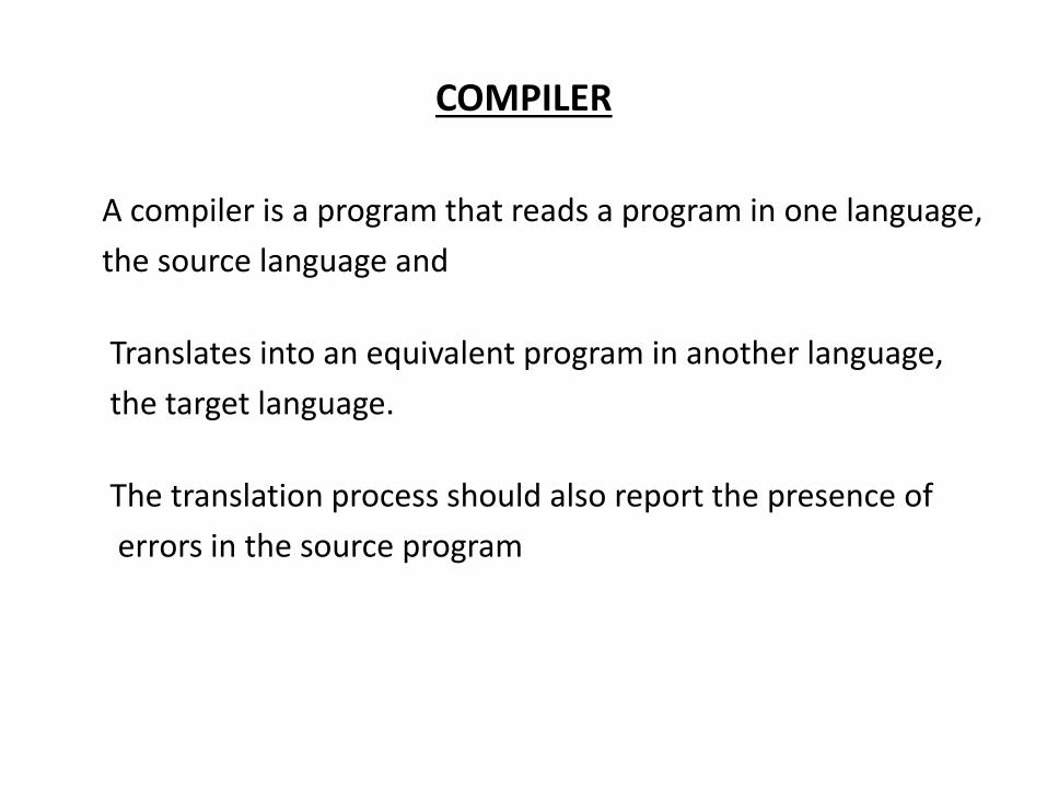
Source

P og a → Co pile → Ta get

Program

↓

Error

Messages

COMPILER

There are two parts of compilation.

. The analysis part breaks up the source program into

constant piece and creates an

intermediate representation of the source program.

The synthesis part constructs the desired target program

from the intermediate representation.

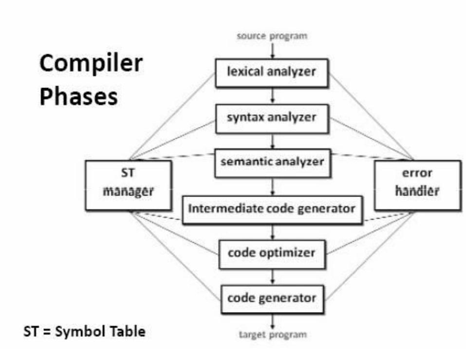
Phases of Compiler

.

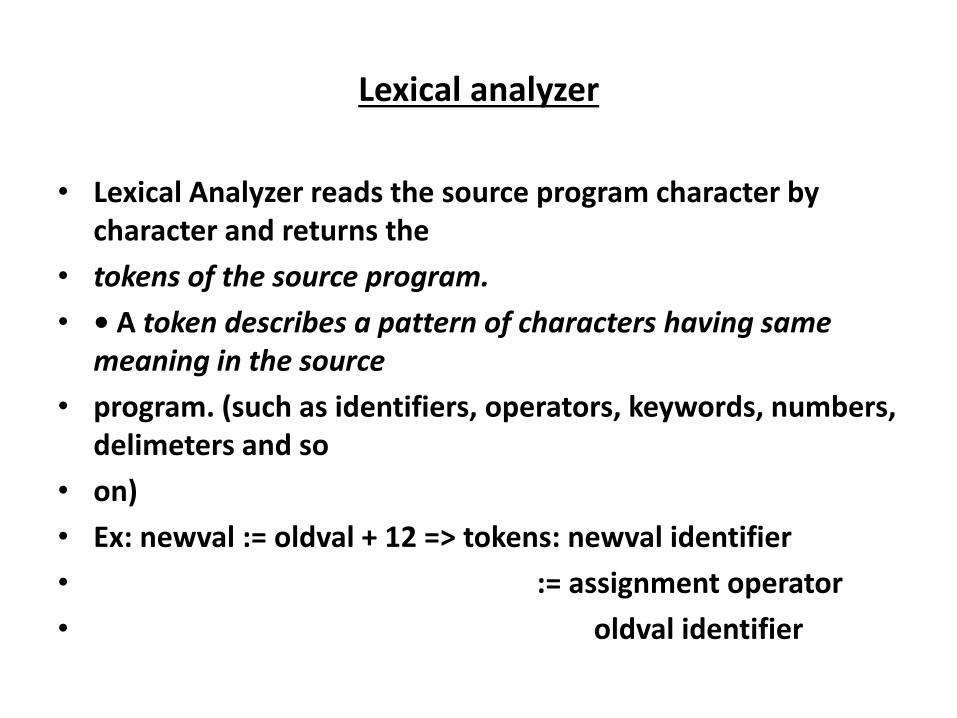
Lexical analyzer

• Lexical Analyzer reads the source program character by

character and returns the

• tokens of the source program.

• • A token describes a pattern of characters having same

meaning in the source

• program. (such as identifiers, operators, keywords, numbers,

delimeters and so

• on)

• Ex: newval := oldval + 12 => tokens: newval identifier

• := assignment operator

• oldval identifier

Lexical analyzer

+

add operator

12 a number

• Puts information about identifiers into the symbol table.

• • ‘egula e p essio s a e used to des i e toke s le i al constructs).

Syntax analyzer

Syntax analyzer.

The syntax of a language is specified by a context free

grammar (CFG).

• The ules i a CFG a e ostl e u si e. • A s ta a al ze he ks hethe a gi e p og a satisfies

the rules implied by a CFG or not.

If it satisfies, the syntax analyzer creates a parse tree for the

given program.

Syntax analyzer

Ex:

We use BNF (Backus Naur Form) to specify a CFG

assgstmt -> identifier := expression

expression -> identifier

expression -> number

expression -> expression + expression

Semantic analyzer

• A semantic analyzer checks the source program for semantic

errors and collects

• the type information for the code generation.

• Type-checking is an important part of semantic analyzer.

• Normally semantic information cannot be represented by a

context-free language

• used in syntax analyzers.

• Context-free grammars used in the syntax analysis are

integrated with attributes

• (semantic rules)

• the result is a syntax-directed translation,

• Attribute grammars

Semantic analyzer

Ex:

newval := oldval + 12

The type of the identifier newval must match with type of

the expression (oldval+12)

Intermediate code generation

A compiler may produce an explicit intermediate codes

representing the source program.

These intermediate codes are generally machine

(architecture independent). But the level of intermediate

codes is close to the level of machine codes.

Intermediate code generation

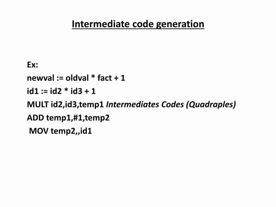
Ex:

newval := oldval * fact + 1

id1 := id2 * id3 + 1

MULT id2,id3,temp1 Intermediates Codes (Quadraples)

ADD temp1,#1,temp2

MOV temp2,,id1

Code optimizer

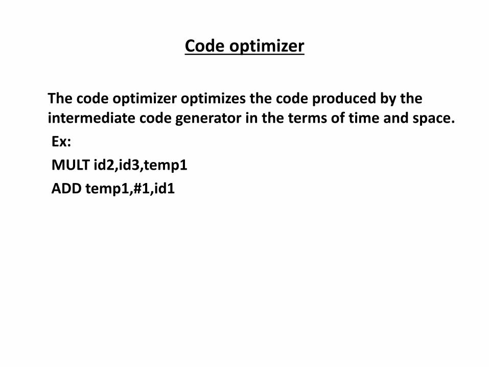
The code optimizer optimizes the code produced by the

intermediate code generator in the terms of time and space.

Ex:

MULT id2,id3,temp1

ADD temp1,#1,id1

Code generator

Produces the target language in a specific architecture.

The target program is normally is a relocatable object file

containing the machine codes.

Ex:

( assume that we have an architecture with instructions

whose at least one of its operands is a machine register)

Code generator

MOVEid2,R1

MULT id3,R1

ADD #1,R1

MOVER1,id1

Compiler construction tools

• A number of tools have been developed variously called

compiler –compiler , compiler generator or translator

writing system

• The input for these systems may contain

• 1. a description of source language.

• 2. a description of what output to be

• generated.

• 3. a description of the target machine.

Compiler construction tools

The principal aids provided by compiler-compiler are

1. Scanner Generator

2. Parser generator

3. Facilities for code generation

Lexical Analyzer

• The Role of the Lexical Analyzer

1st phase of compiler

Reads i/p character & produce o/p sequence of tokens that

the Parser uses for syntax analysis

It can either work as a separate module or as sub module

Tokens , Patterns and Lexemes

• Lexeme: Sequence of character in the source pm that is

matched against the pattern for a token

• Pattern: The rule associated with each set of strings is called

pattern.

• Lexeme is matched against pattern to generate token

• Token: Token is word, which describes the lexeme in source

pgm. It is generated when lexeme is matched against pattern

3 Methods of constructing Lexical Analyzer

. • 1. Using Lexical Code Generator

• Such compilers/ tools are available that takes in Regular

Expressions

• As i/p and generate code for that R.E.These tools can be

used to generate Lexical Analyzer code from R.Es

• - Example of such Tool is LEX for Unix .

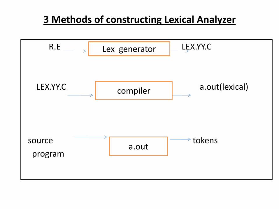
3 Methods of constructing Lexical Analyzer

R.E LEX.YY.C

LEX.YY.C a.out(lexical)

source tokens

program

Lex generator

compiler

a.out

Compiler and Translator

• Compiler is a form of translator that translate a program

itte i o e la guage

• The “ou e La guage to a e ui ale t p og a i a se o d la guage The Ta get

• la guage o The O je t La guage

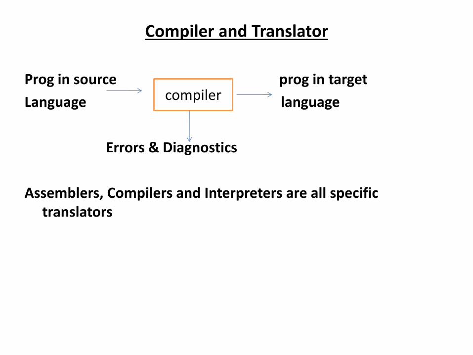
Compiler and Translator

Prog in source prog in target

Language language

Errors & Diagnostics

Assemblers, Compilers and Interpreters are all specific

translators

compiler

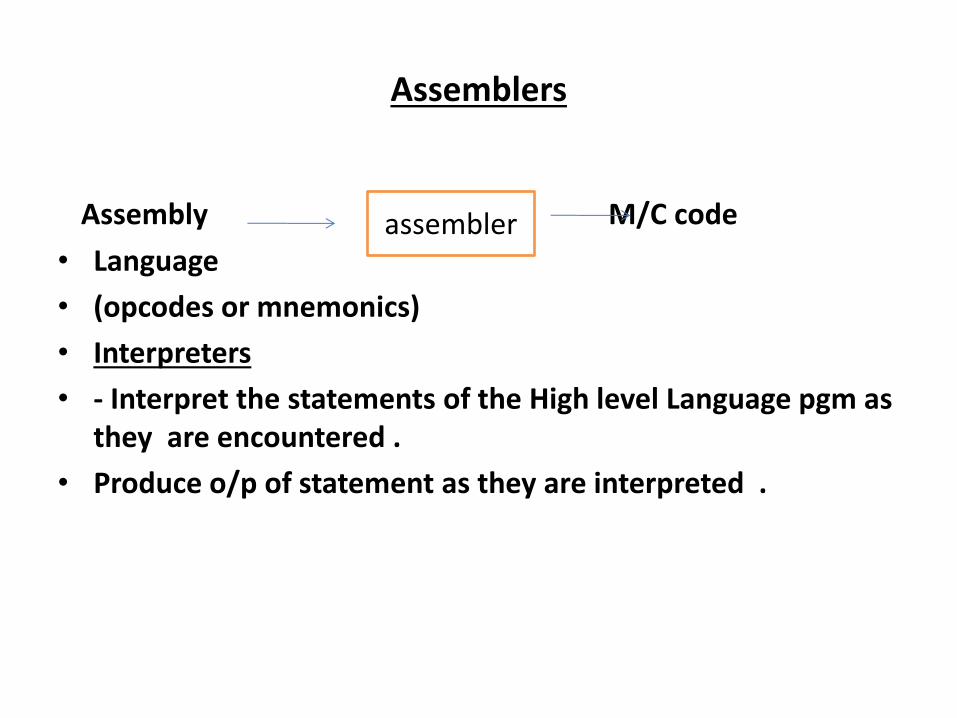
Assemblers

Assembly M/C code

• Language

• (opcodes or mnemonics)

• Interpreters

• - Interpret the statements of the High level Language pgm as

they are encountered .

• Produce o/p of statement as they are interpreted .

assembler

Languages involved in Compiler

3 languages are involved in a compiler

• 1. Source language: Read by compiler

• 2. Target or Object language : translated by compiler

/translator to another language

• 4. Host Language: Language in which compiler is written

Advantages of Compiler

• Conciseness which improves programmer productivity,

• semantic restriction

• Translate and analyze H.L.L.(source pgm) only once and then

• run the equivalent m/c code produce by compiler

Disadvantage of Compiler

• Slower speed

• Size of compiler and compiled code

• Debugging involves all source code

Interpreter versus Compiler

Compiler translates to machine code

Interpreter

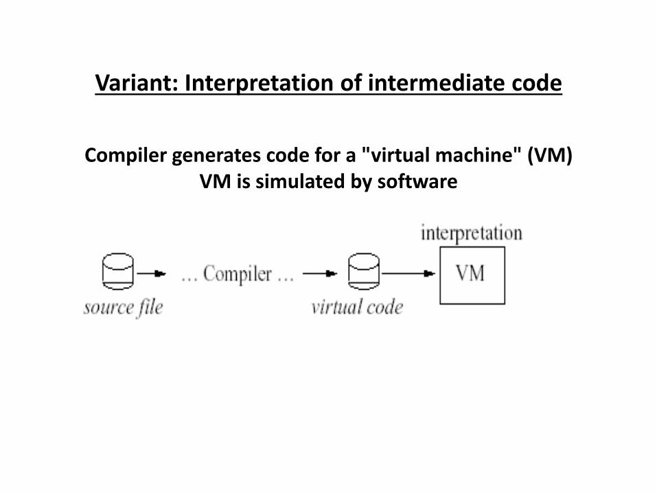
Variant: Interpretation of intermediate code

Compiler generates code for a "virtual machine" (VM)

VM is simulated by software

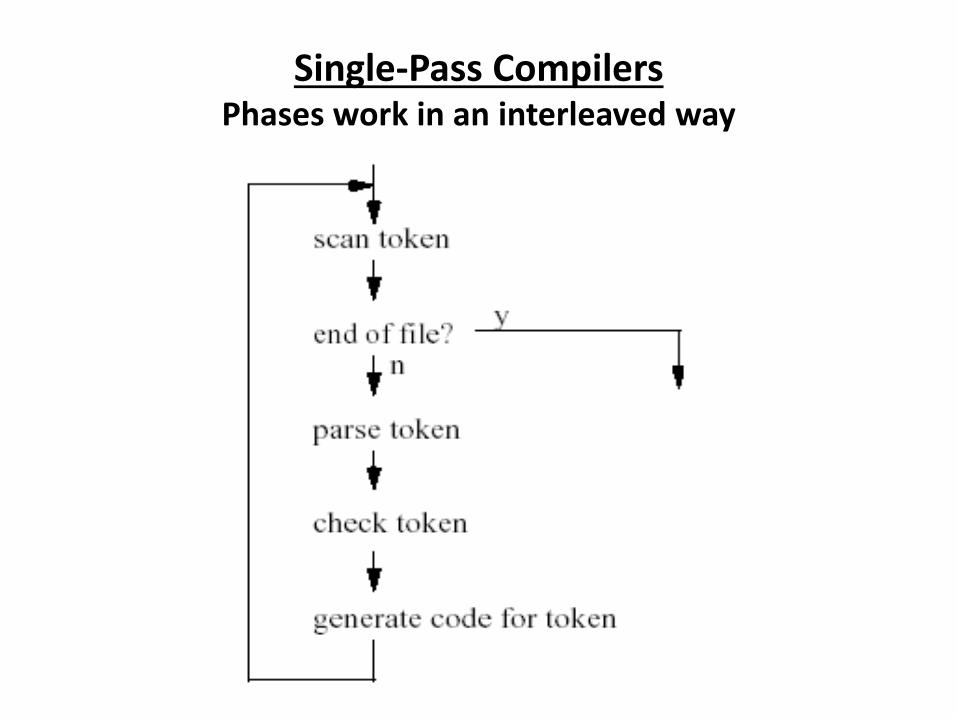
Single-Pass Compilers Phases work in an interleaved way

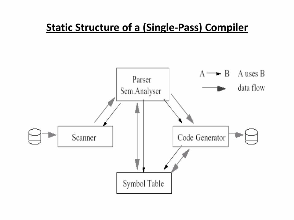
Static Structure of a (Single-Pass) Compiler

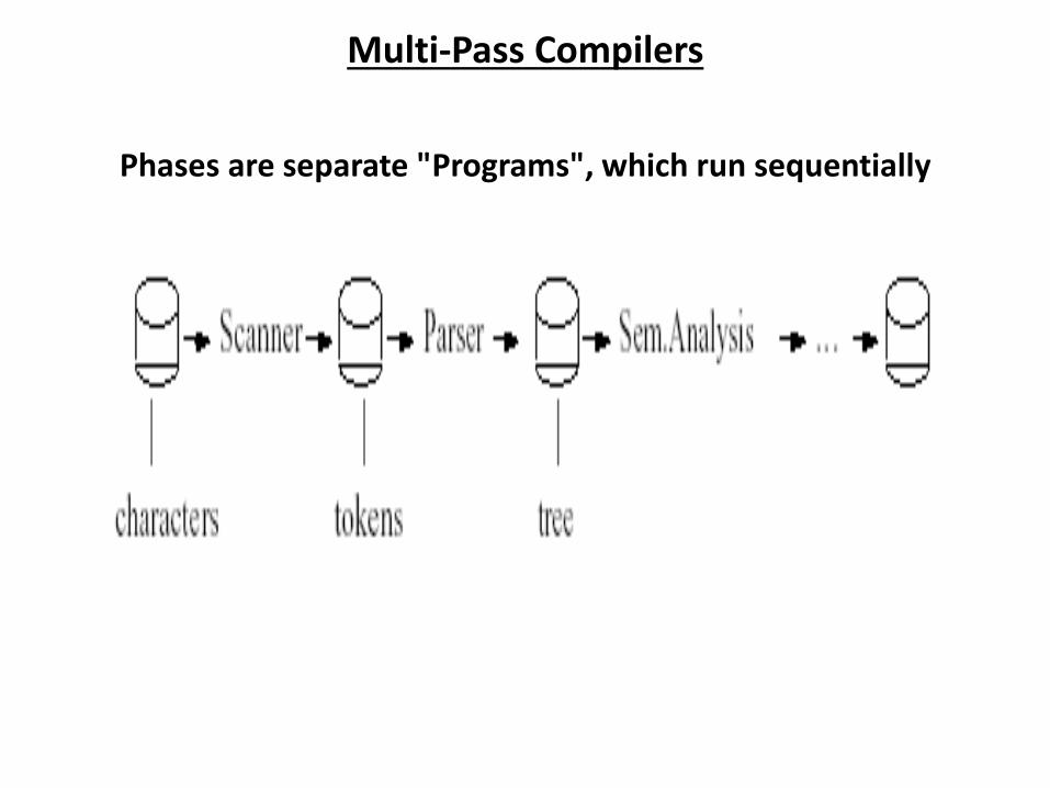
Multi-Pass Compilers

Phases are separate "Programs", which run sequentially

Why multi-pass?

If memory is scarce (irrelevant today)

If the language is complex

If portability is important

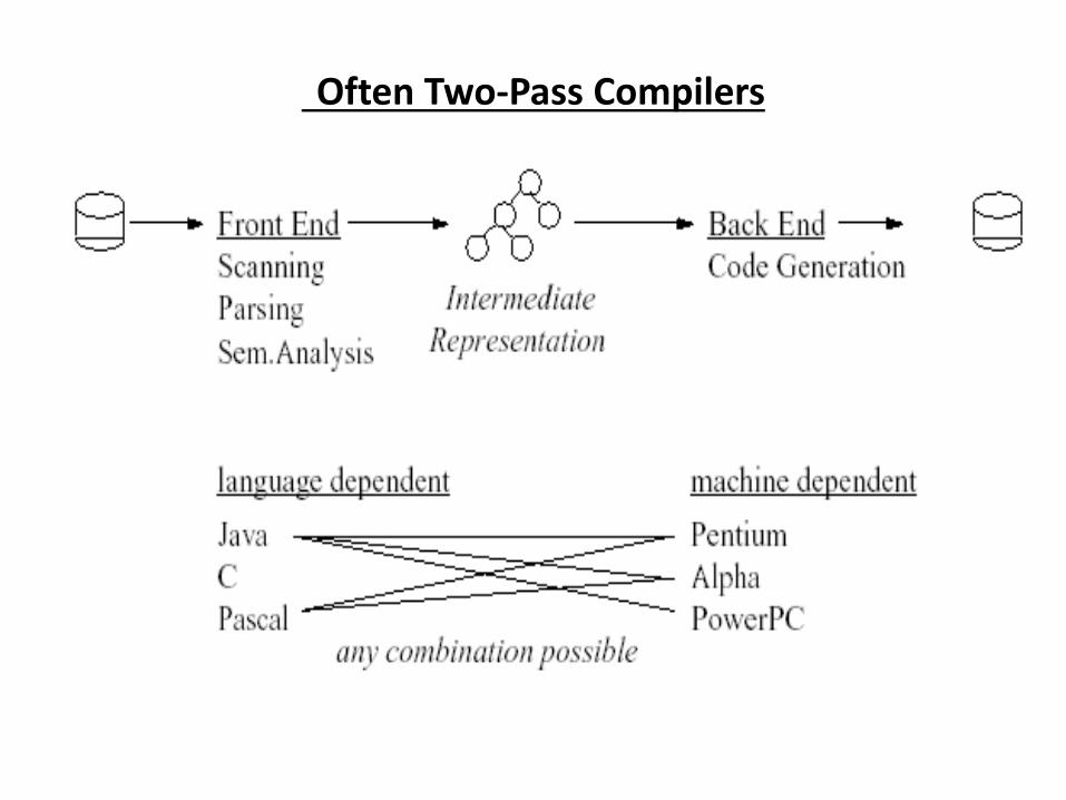
Often Two-Pass Compilers

Loader/Linker Editor:

Performs 2 functions

• i. Loading : relocatable code is converted to absolute code

i.e. placed at their specified position

ii. Link-Editor :

Make single pgm from several files of relocatable

m/c code.

The file may be o/p of different compilation .

May be Library files or routine provided by system .

Result is executable file

Preprocessor

Produce i/p to compiler. They may perform

i. Macro processing: shorthand for longer construct .

ii. File inclusion: separate module can be used by including

their file e.g #include <iostream> .

iii. Rational preprocessors: give support for additional

facilities which are not included in compiler itself .

iv. Language Extension: may include extra capabilities .

Major Types of Compiler

• 1. Self-resident Compiler: generates Target code for the

same m/c or host .

• 2. Cross Compilers: generates target code for m/c other then

host .

Phases and passes

• In logical terms a compiler is thought of as consisting of

stages and phases

• Physically it is made up of passes

• The compiler has one pass for each time the source code, or

a representation of

• it, is read

• Many compilers have just a single pass so that the complete

compilation

• process is performed while the code is read once

Phases and passes

• The various phases described will therefore be executed in

parallel

• Earlier compilers had a large number of passes, typically due

to the limited

• memory space available

• Modern compilers are single pass since memory space is not

usually a problem

Use of tools

• The 2 main types of tools used in compiler production are:

• 1. a lexical analyzer generator

• Takes as input the lexical structure of a language, which defines how its

• tokens are made up from characters

• Produces as output a lexical analyzer (a program in C for example) for the

• language

• Unix lexical analyzer Lex

• 2. a symbol analyzer generator

Use of tools

• Takes as input the syntactical definition of a language

• Produces as output a syntax analyzer (a program in C for

example) for the

• language

• The most widely know is the Unix-based YACC (Yet

Another

• Compiler-Compiler), used in conjunction with Lex.

• Bison: public domain version

Applications of compiler techniques

• Compiler technology is useful for a more general class of applications

• Many programs share the basic properties of compilers: they read textual input,

• organize it into a hierarchical structure and then process the structure

• An understanding how programming language compilers are designed and

• organized can make it easier to implement these compiler like applications as

• well

• More importantly, tools designed for compiler writing such as lexical analyzer

Applications of compiler techniqu

• generators and parser generators can make it vastly easier to implement such

• applications

• Thus, compiler techniques - An important knowledge for computer science

• engineers

• Examples:

• Document processing: Latex, HTML, XML

• User interfaces: interactive applications, file systems, databases

• Natural language treatment

• Automata Theory, La

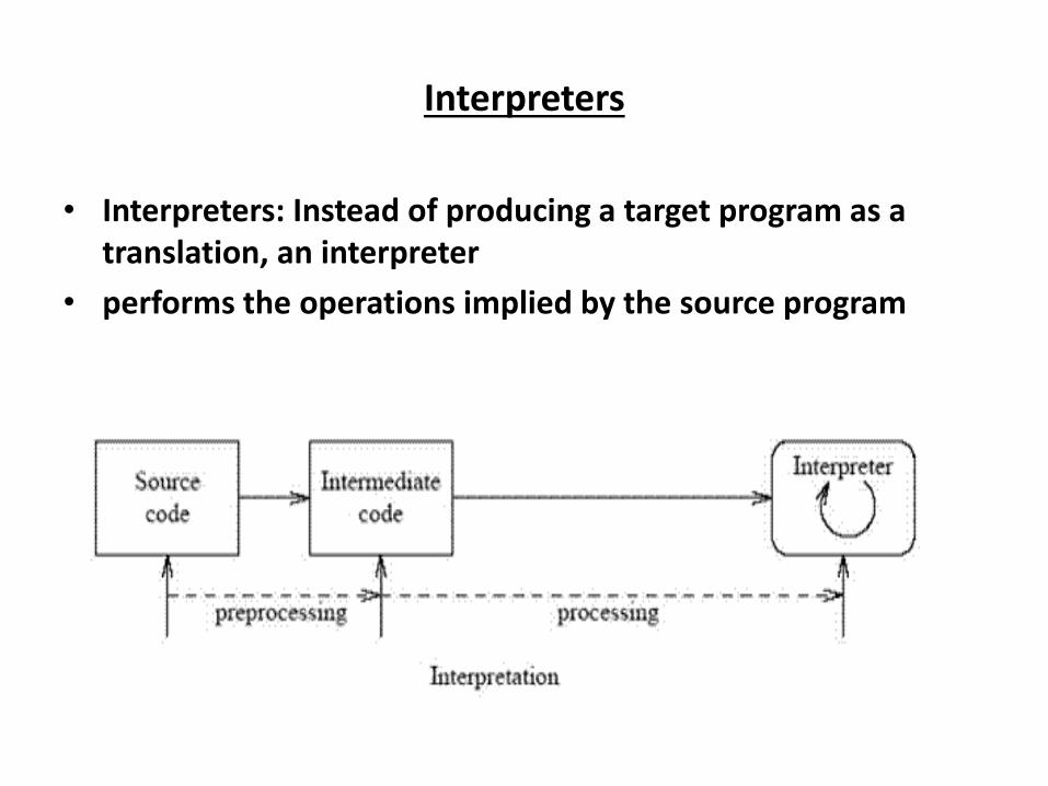
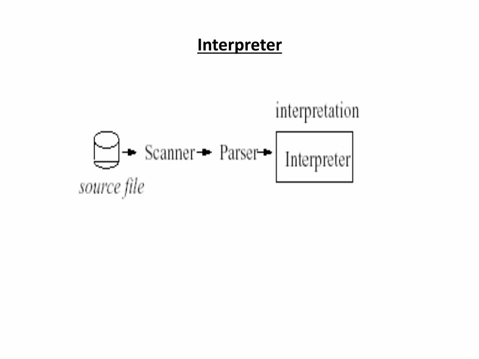
Interpreters

• Interpreters: Instead of producing a target program as a

translation, an interpreter

• performs the operations implied by the source program

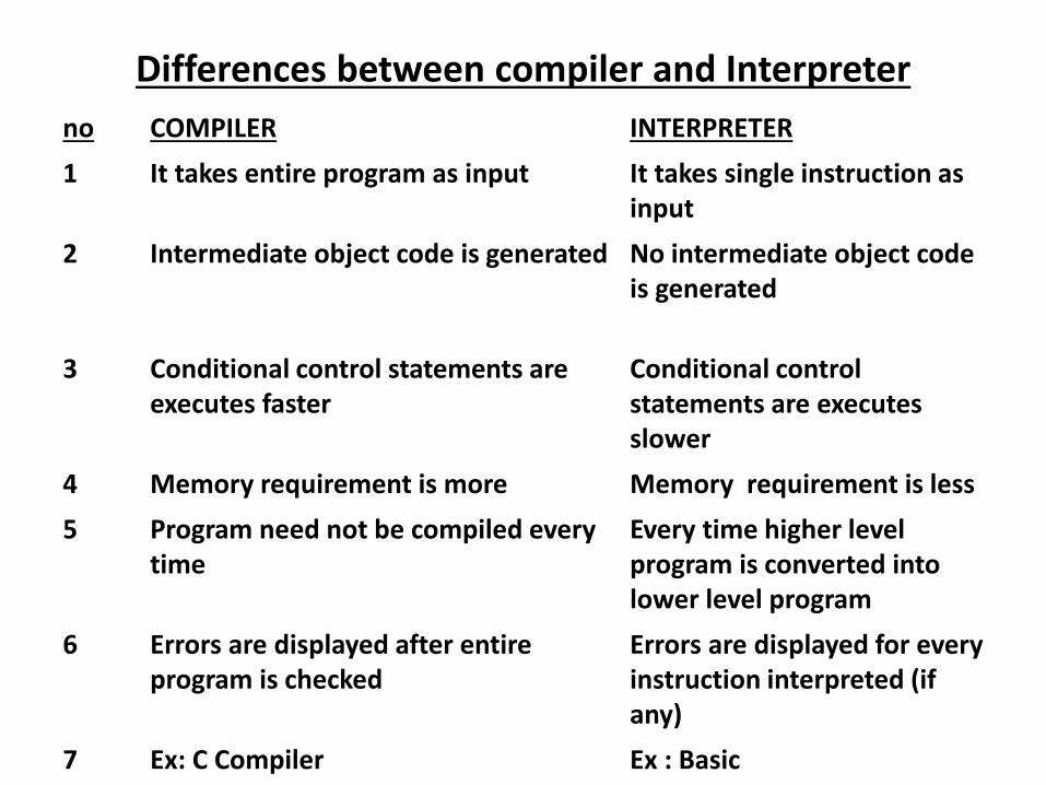
Differences between compiler and Interpreter

no COMPILER INTERPRETER

1 It takes entire program as input It takes single instruction as

input

2 Intermediate object code is generated No intermediate object code

is generated

3 Conditional control statements are

executes faster

Conditional control

statements are executes

slower

4 Memory requirement is more Memory requirement is less

5 Program need not be compiled every

time

Every time higher level

program is converted into

lower level program

6 Errors are displayed after entire

program is checked

Errors are displayed for every

instruction interpreted (if

any)

7 Ex: C Compiler Ex : Basic

Types of compilers

1.Incremental compiler :

It is a compiler it performs the recompilation of only modified

source rather than compiling the whole source program.

Features:

1.It tracks the dependencies between output and source

program.

2.It produces the same result as full recompilation.

3.It performs less task than recompilation.

4.The process of incremental compilation is effective for

maintenance.

Types of compilers

2.Cross compiler:

Basically there exists 3 languages

1.source language i.e application program.

2.Target language in which machine code is return.

3.Implementation language in which a compiler is

return.

All these 3 languages are different. In other words

there may be a compiler which run on one machine and

produces the target code for another machine. Such a

compiler is called cross compiler.

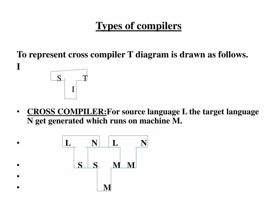
Types of compilers

To represent cross compiler T diagram is drawn as follows.

I

S T

I

• CROSS COMPILER:For source language L the target language N get generated which runs on machine M.

• L N L N

• S S M M

•

• M

Bootstrapping Compilers and T-diagrams

• The rules for T-diagrams are very simple. A compiler written

i so e la guage C ould e a thi g f o a hi e ode on up) that translates programs in language A to language B

looks like this (these diagrams are from

Bootstrapping Compilers and T-diagrams

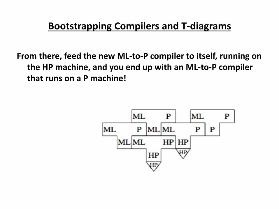
• Now suppose you have a machine that can directly run HP

machine code, and a compiler from ML to HP machine code,

and you want to get a ML compiler running on different

machine code P. You can start by writing an ML-to-P

compiler in ML, and compile that to get an ML-to-P compiler

in HP:

Bootstrapping Compilers and T-diagrams

From there, feed the new ML-to-P compiler to itself, running on

the HP machine, and you end up with an ML-to-P compiler

that runs on a P machine!

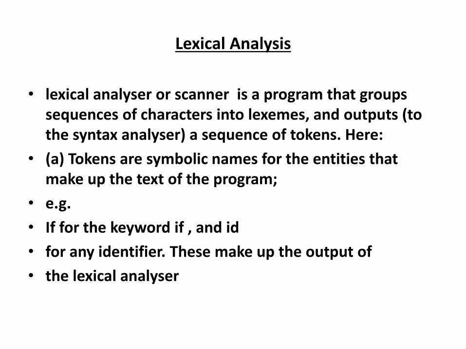
Lexical Analysis

• lexical analyser or scanner is a program that groups

sequences of characters into lexemes, and outputs (to

the syntax analyser) a sequence of tokens. Here:

• (a) Tokens are symbolic names for the entities that

make up the text of the program;

• e.g.

• If for the keyword if , and id

• for any identifier. These make up the output of

• the lexical analyser

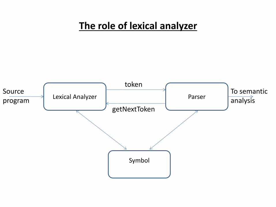
The role of lexical analyzer

Lexical Analyzer Parser Source

program

token

getNextToken

Symbol

table

To semantic

analysis

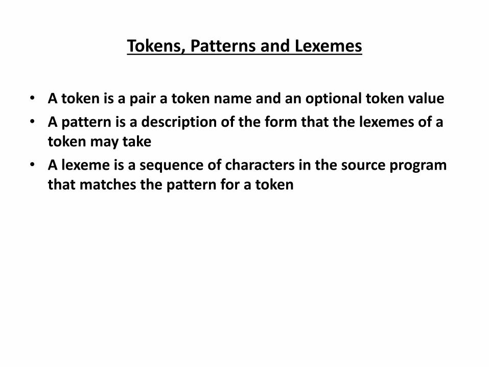
Tokens, Patterns and Lexemes

• A token is a pair a token name and an optional token value

• A pattern is a description of the form that the lexemes of a

token may take

• A lexeme is a sequence of characters in the source program

that matches the pattern for a token

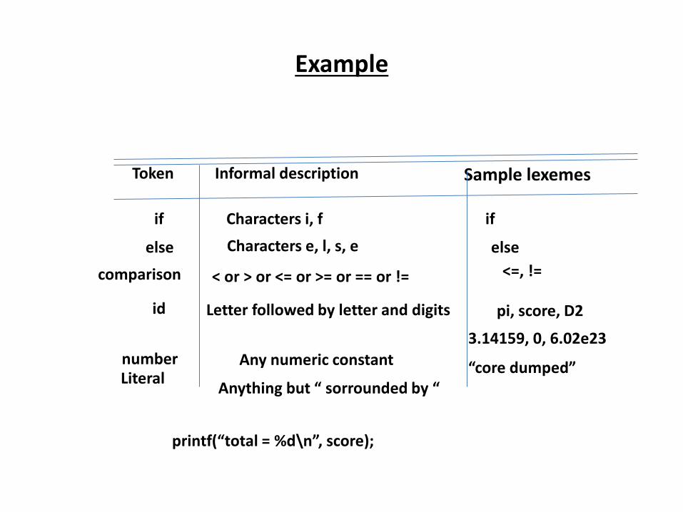
Example

Token Informal description Sample lexemes

if

else

comparison

id

number Literal

Characters i, f

Characters e, l, s, e

< or > or <= or >= or == or !=

Letter followed by letter and digits

Any numeric constant

Anything ut so ou ded

if

else

<=, !=

pi, score, D2

3.14159, 0, 6.02e23

o e du ped

p i tf total = %d\ , s o e ;

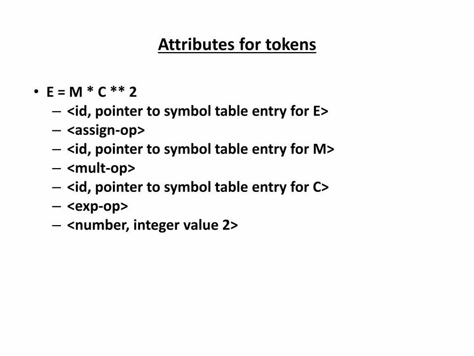
Attributes for tokens

• E = M * C ** 2

– <id, pointer to symbol table entry for E>

– <assign-op>

– <id, pointer to symbol table entry for M>

– <mult-op>

– <id, pointer to symbol table entry for C>

– <exp-op>

– <number, integer value 2>

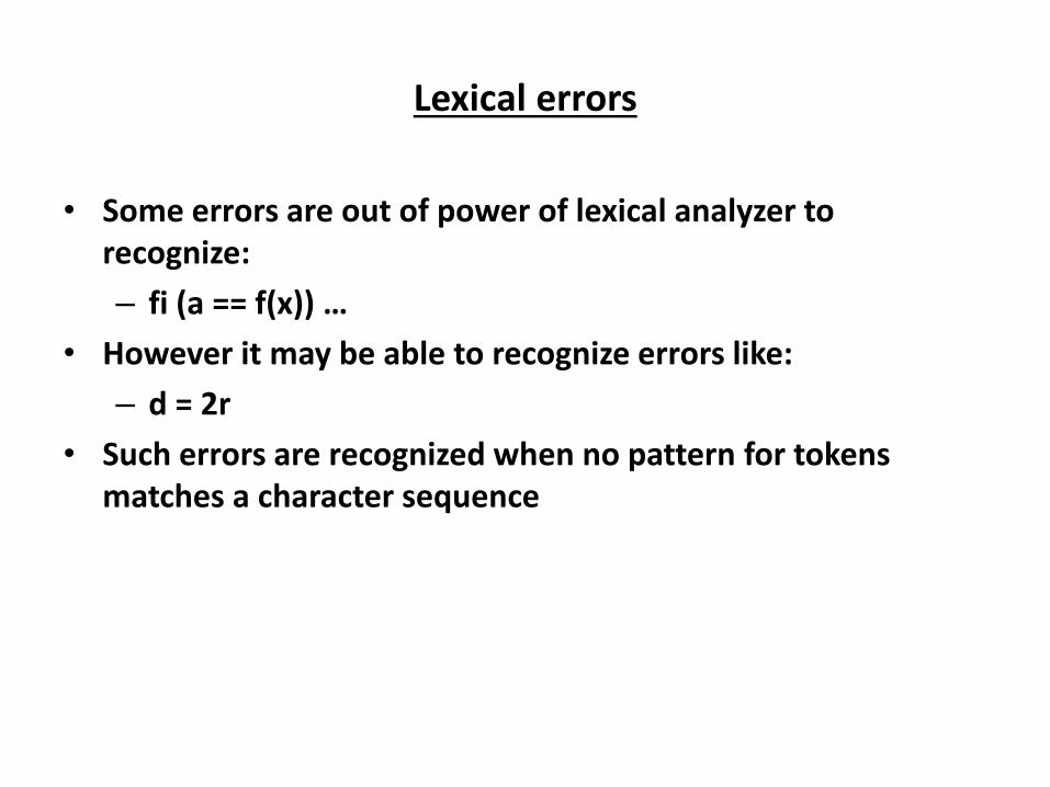
Lexical errors

• Some errors are out of power of lexical analyzer to

recognize:

– fi a == f …

• However it may be able to recognize errors like:

– d = 2r

• Such errors are recognized when no pattern for tokens

matches a character sequence

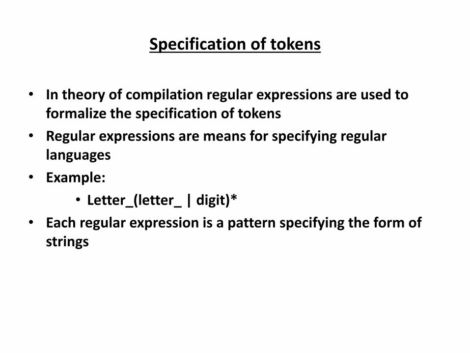
Specification of tokens

• In theory of compilation regular expressions are used to

formalize the specification of tokens

• Regular expressions are means for specifying regular

languages

• Example:

• Letter_(letter_ | digit)*

• Each regular expression is a pattern specifying the form of

strings

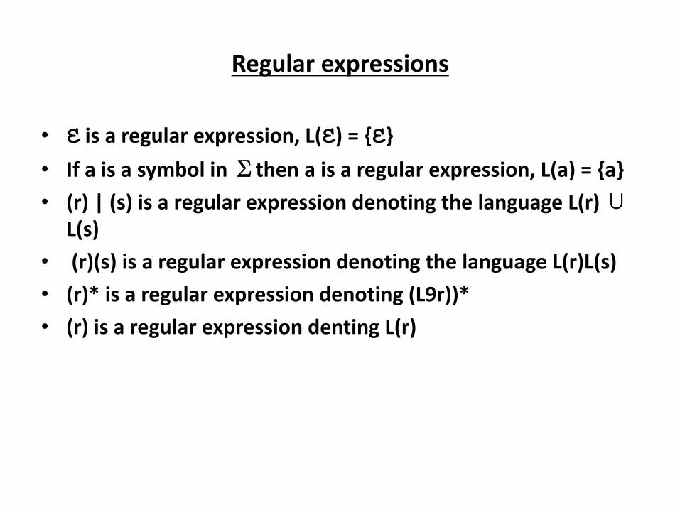
Regular expressions

• Ɛ is a regular expression, L(Ɛ) = {Ɛ}

• If a is a symbol in ∑then a is a regular expression, L(a) = {a}

• (r) | (s) is a regular expression denoting the language L(r) ∪ L(s)

• (r)(s) is a regular expression denoting the language L(r)L(s)

• (r)* is a regular expression denoting (L9r))*

• (r) is a regular expression denting L(r)

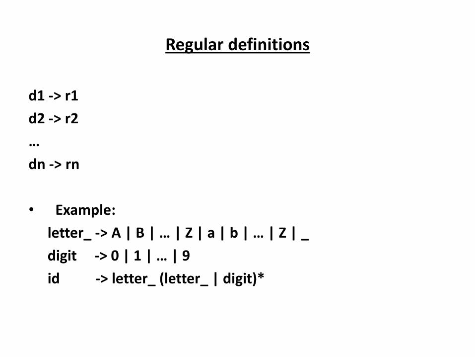
Regular definitions

d1 -> r1

d2 -> r2

…

dn -> rn

• Example:

letter_ -> A | B | … | Z | a | b | … | Z | _

digit -> 0 | 1 | … | 9

id -> letter_ (letter_ | digit)*

Extensions

• One or more instances: (r)+

• Zero of one instances: r?

• Character classes: [abc]

• Example:

– letter_ -> [A-Za-z_]

– digit -> [0-9]

– id -> letter_(letter|digit)*

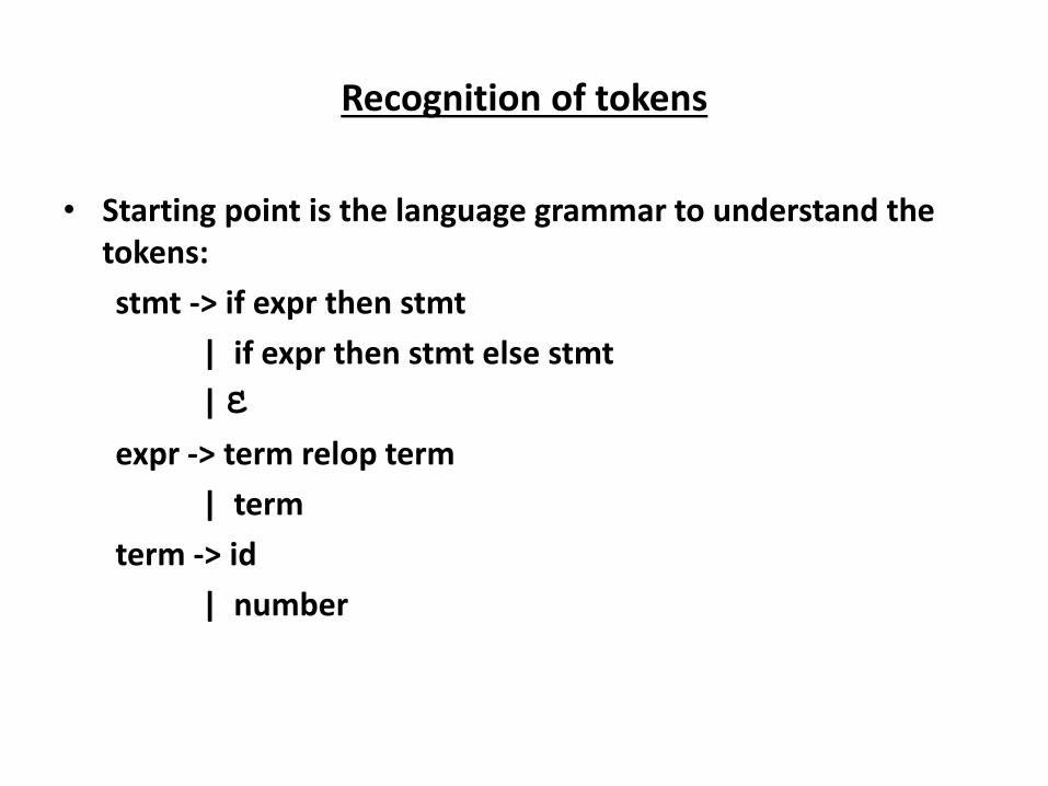
Recognition of tokens

• Starting point is the language grammar to understand the

tokens:

stmt -> if expr then stmt

| if expr then stmt else stmt

| Ɛ

expr -> term relop term

| term

term -> id

| number

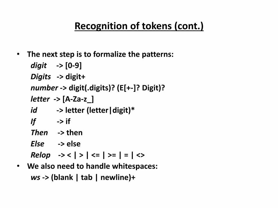
Recognition of tokens (cont.)

• The next step is to formalize the patterns:

digit -> [0-9]

Digits -> digit+

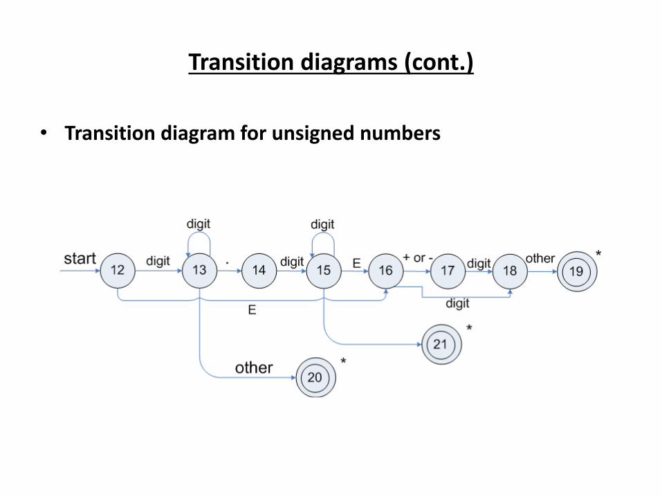
number -> digit(.digits)? (E[+-]? Digit)?

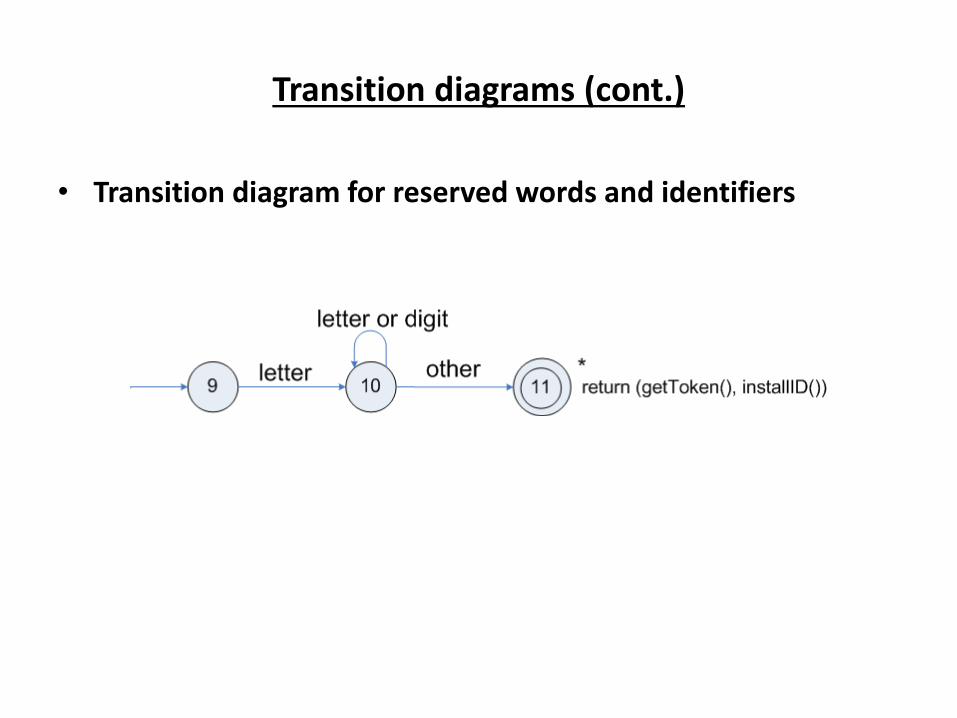
letter -> [A-Za-z_]

id -> letter (letter|digit)*

If -> if

Then -> then

Else -> else

Relop -> < | > | <= | >= | = | <>

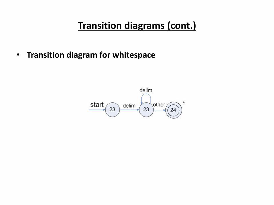
• We also need to handle whitespaces:

ws -> (blank | tab | newline)+

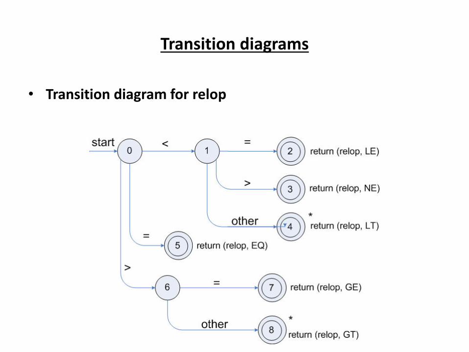
Transition diagrams

• Transition diagram for relop

Transition diagrams (cont.)

• Transition diagram for reserved words and identifiers

Transition diagrams (cont.)

• Transition diagram for unsigned numbers

Transition diagrams (cont.)

• Transition diagram for whitespace

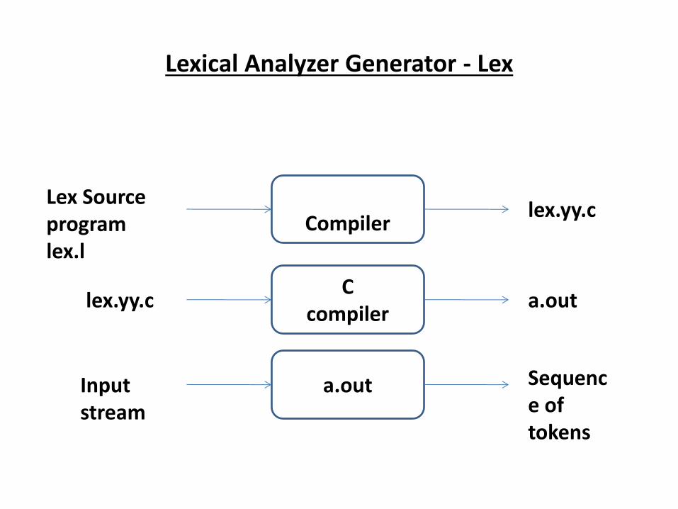
Lexical Analyzer Generator - Lex

Lexical

Compiler

Lex Source

program

lex.l

lex.yy.c

C

compiler lex.yy.c a.out

a.out Input

stream

Sequenc

e of

tokens

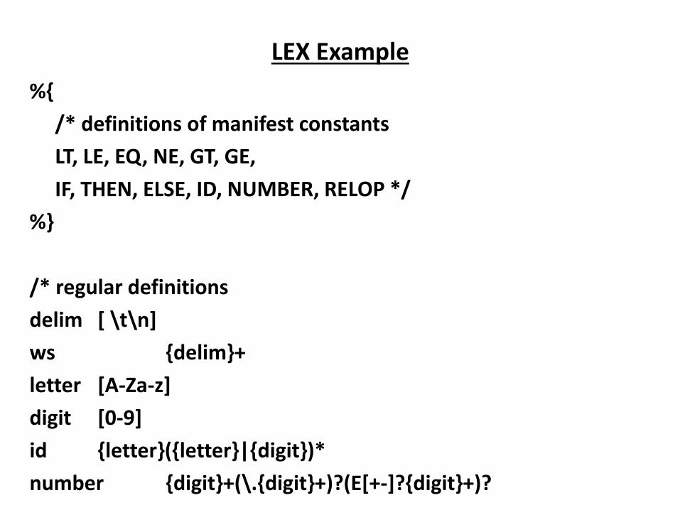
LEX Example

%{

/* definitions of manifest constants

LT, LE, EQ, NE, GT, GE,

IF, THEN, ELSE, ID, NUMBER, RELOP */

%}

/* regular definitions

delim [ \t\n]

ws {delim}+

letter [A-Za-z]

digit [0-9]

id {letter}({letter}|{digit})*

number {digit}+(\.{digit}+)?(E[+-]?{digit}+)?

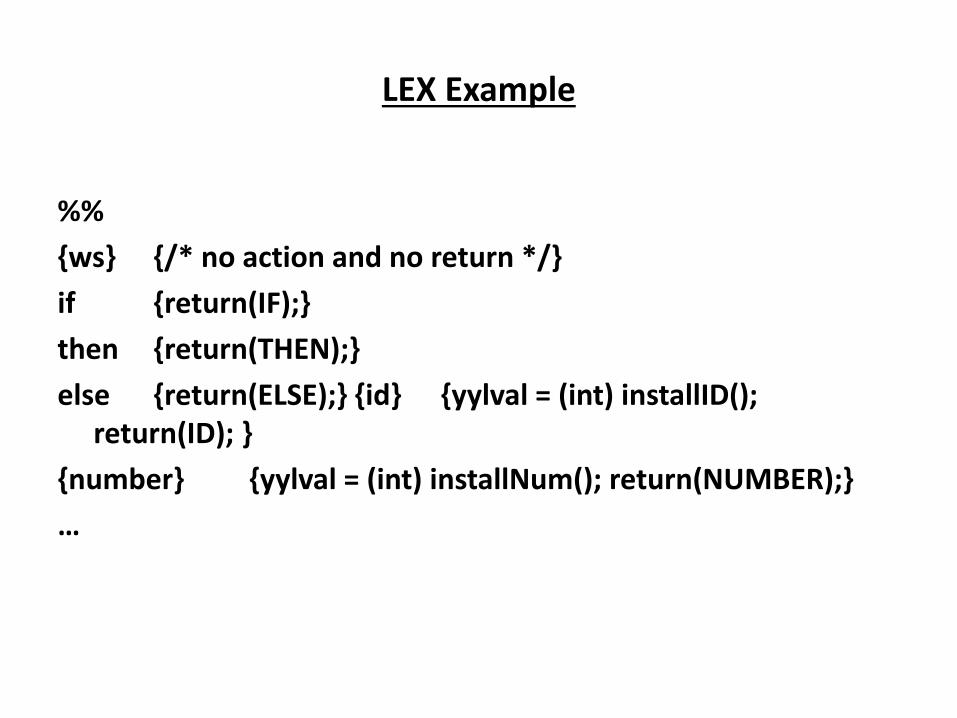
LEX Example

%%

{ws} {/* no action and no return */}

if {return(IF);}

then {return(THEN);}

else {return(ELSE);} {id} {yylval = (int) installID();

return(ID); }

{number} {yylval = (int) installNum(); return(NUMBER);}

…

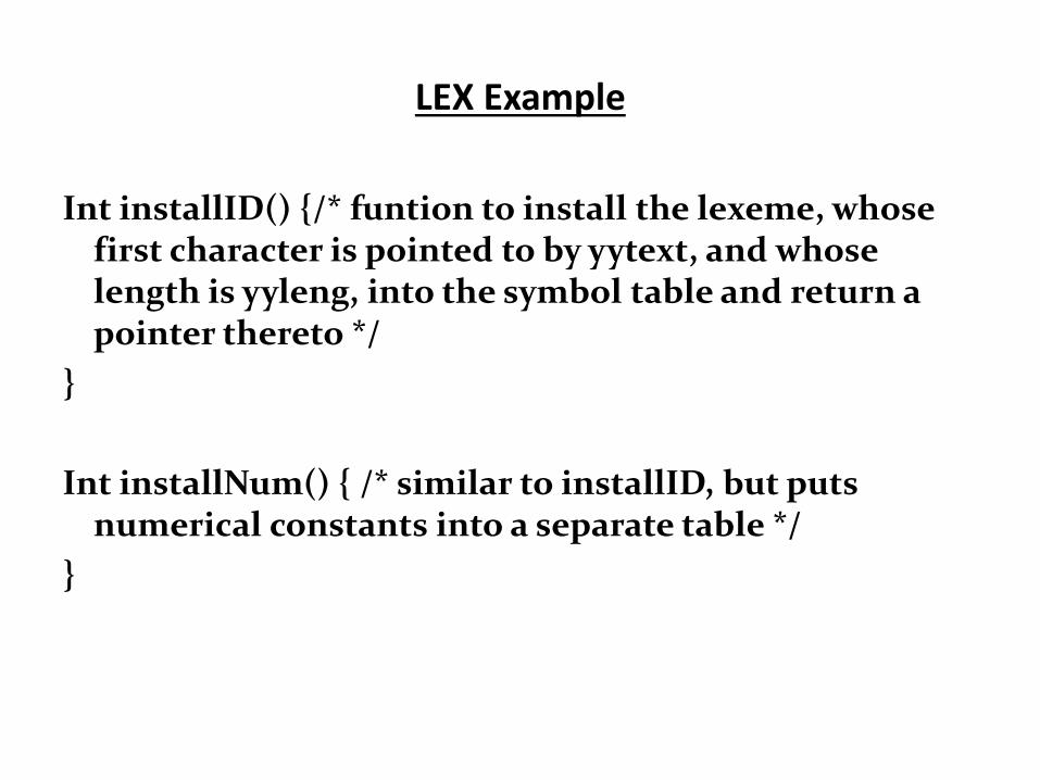
LEX Example

Int installID() {/* funtion to install the lexeme, whose first character is pointed to by yytext, and whose length is yyleng, into the symbol table and return a pointer thereto */

}

Int installNum() { /* similar to installID, but puts numerical constants into a separate table */

}

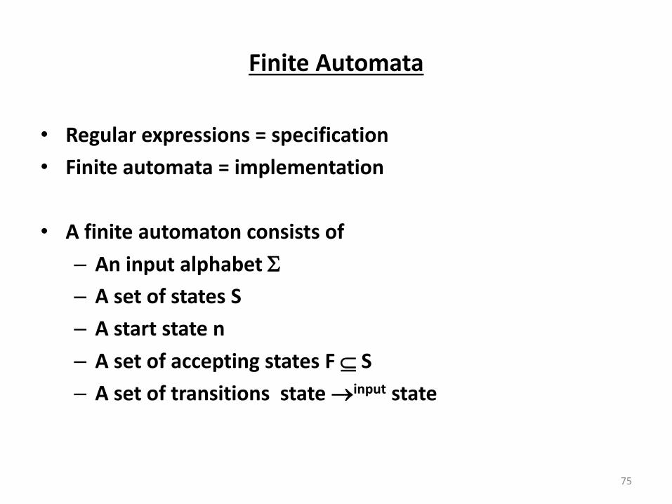
Finite Automata

• Regular expressions = specification

• Finite automata = implementation

• A finite automaton consists of

– An input alphabet

– A set of states S

– A start state n

– A set of accepting states F S

– A set of transitions state input state

75

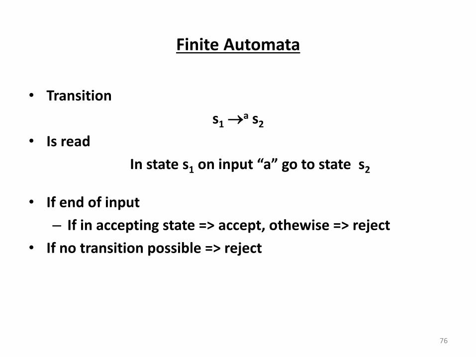
Finite Automata

• Transition

s1 a s2

• Is read

In state s1 o i put a go to state s2

• If end of input

– If in accepting state => accept, othewise => reject

• If no transition possible => reject

76

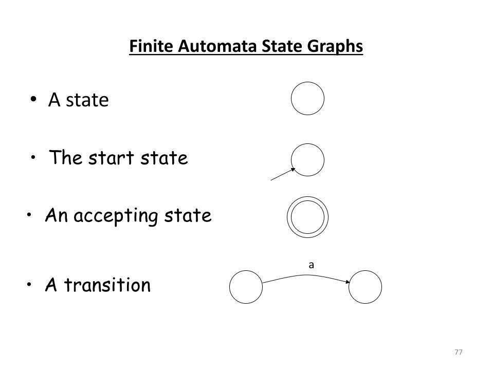
Finite Automata State Graphs

• A state

77

• The start state

• An accepting state

• A transition a

Example

• Alphabet {0,1}

• What language does this recognize?

78

0

1

0

1

0

1

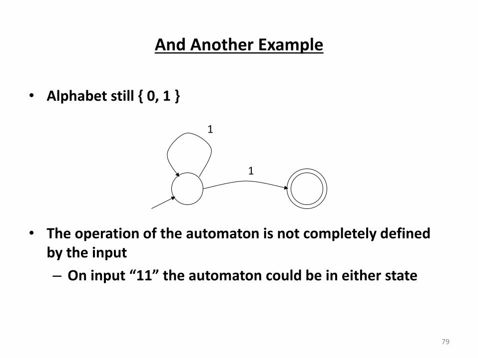
And Another Example

• Alphabet still { 0, 1 }

• The operation of the automaton is not completely defined

by the input

– O i put the auto ato ould e i eithe state

79

1

1

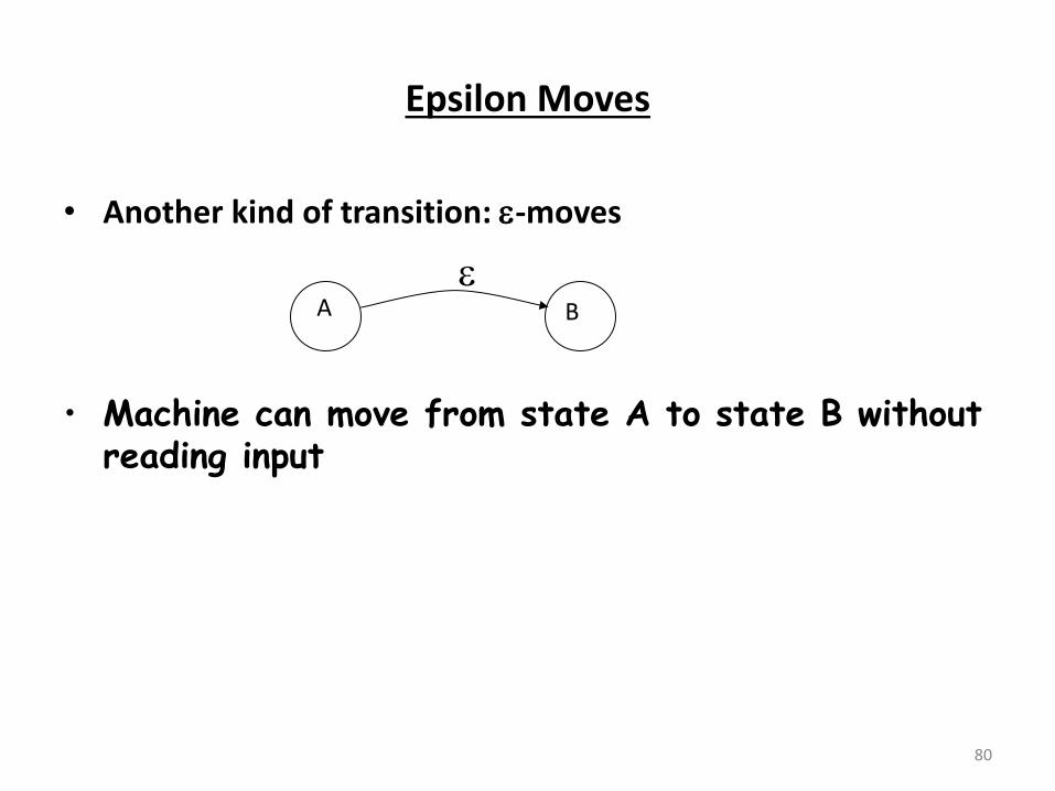
Epsilon Moves

• Another kind of transition: -moves

80

• Machine can move from state A to state B without reading input

A B

Deterministic and Nondeterministic Automata

• Deterministic Finite Automata (DFA)

– One transition per input per state

– No -moves

• Nondeterministic Finite Automata (NFA)

– Can have multiple transitions for one input in a given

state

– Can have -moves

• Finite automata have finite memory

– Need only to encode the current state

81

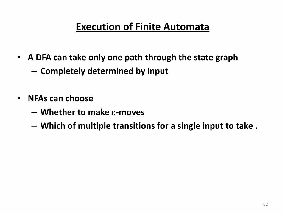
Execution of Finite Automata

• A DFA can take only one path through the state graph

– Completely determined by input

• NFAs can choose

– Whether to make -moves

– Which of multiple transitions for a single input to take .

82

Acceptance of NFAs

• An NFA can get into multiple states

83

• Input:

0

1

1

0

1 0 1

• Rule: NFA accepts if it can get in a final state

NFA vs. DFA (1)

• NFAs and DFAs recognize the same set of languages (regular

languages)

• DFAs are easier to implement

– There are no choices to consider

84

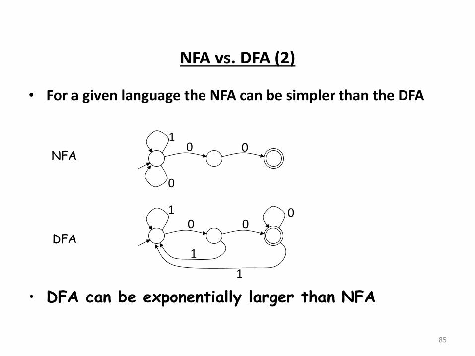
NFA vs. DFA (2)

• For a given language the NFA can be simpler than the DFA

85

0 1

0

0

0 1

0

1

0

1

NFA

DFA

• DFA can be exponentially larger than NFA

Regular Expressions to Finite Automata

• High-level sketch

86

Regular expressions

NFA

DFA

Lexical Specification

Table-driven Implementation of DFA

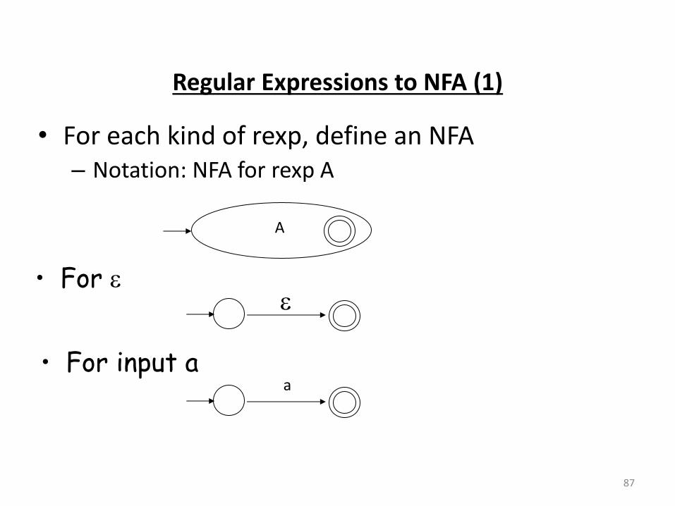
Regular Expressions to NFA (1)

• For each kind of rexp, define an NFA

– Notation: NFA for rexp A

87

A

• For

• For input a a

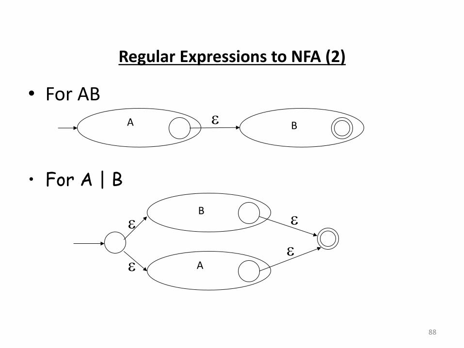
Regular Expressions to NFA (2)

• For AB

88

A B

• For A | B

A

B

Regular Expressions to NFA (3)

• For A*

89

A

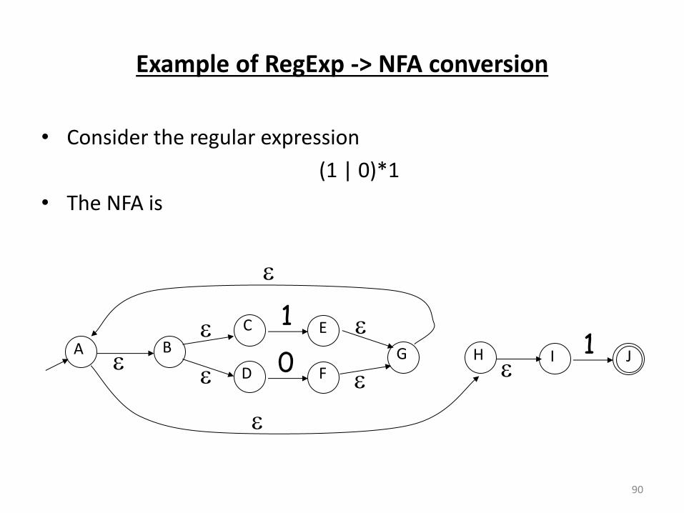
Example of RegExp -> NFA conversion

• Consider the regular expression

(1 | 0)*1

• The NFA is

90

1 C E

0 D F

B

G

A H 1 I J

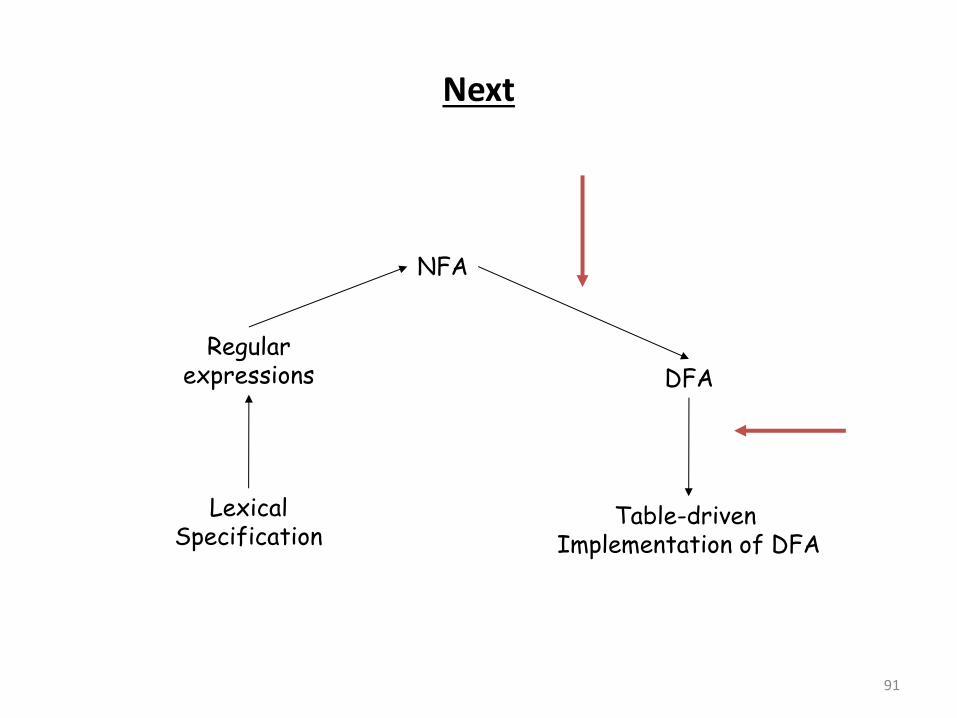
Next

91

Regular expressions

NFA

DFA

Lexical Specification

Table-driven Implementation of DFA

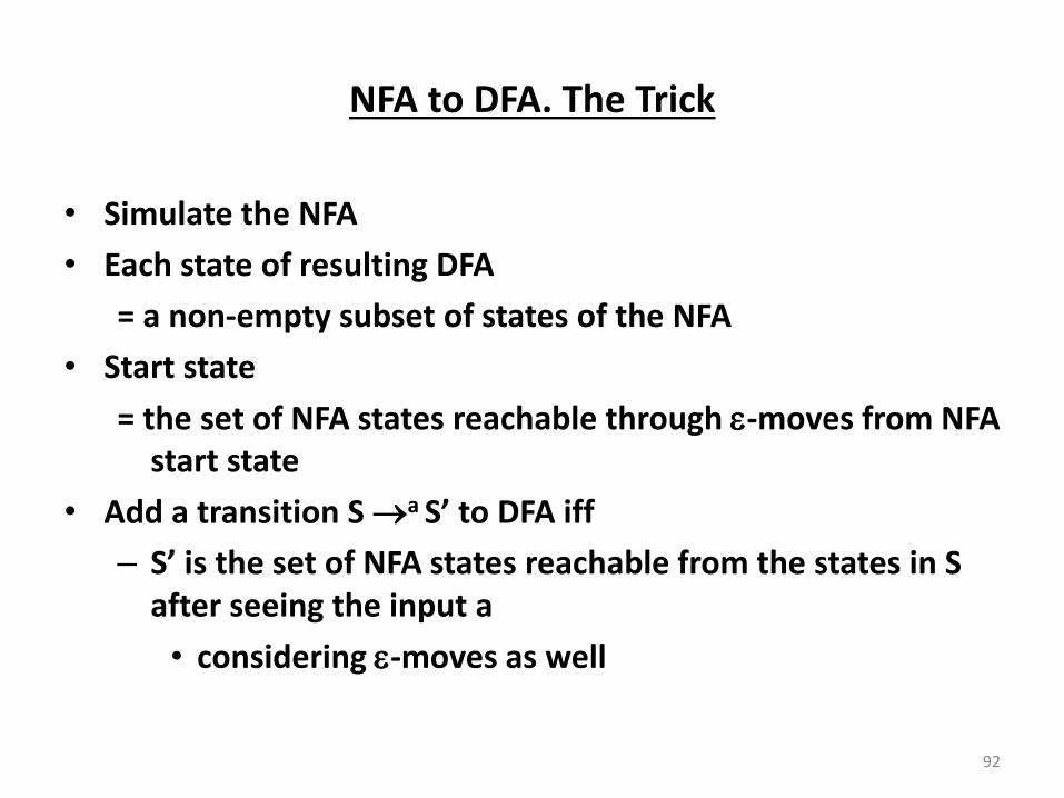
NFA to DFA. The Trick

• Simulate the NFA

• Each state of resulting DFA

= a non-empty subset of states of the NFA

• Start state

= the set of NFA states reachable through -moves from NFA

start state

• Add a transition S a “ to DFA iff – “ is the set of NFA states ea ha le f o the states i “

after seeing the input a

• considering -moves as well

92

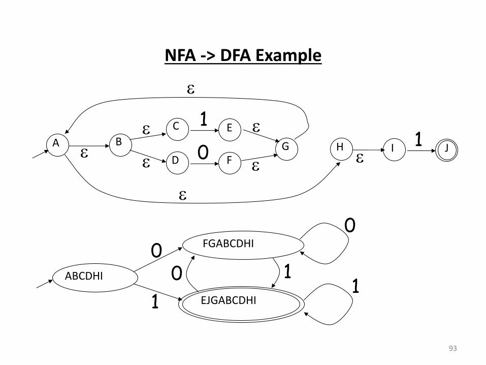
NFA -> DFA Example

93

1

0 1

A B

C

D

E

F G H I J

ABCDHI

FGABCDHI

EJGABCDHI

0

1

0

1 0 1

NFA to DFA. Remark

• An NFA may be in many states at any time

• How many different states ?

• If there are N states, the NFA must be in some subset of

those N states

• How many non-empty subsets are there?

– 2N - 1 = finitely many, but exponentially many

94

Implementation

• A DFA can be implemented by a 2D table T

– O e di e sio is states

– Othe di e sio is i put s ols

– For every transition Si a Sk define T[i,a] = k

• DFA e e utio

– If in state Si and input a, read T[i,a] = k and skip to state Sk

– Very efficient

95

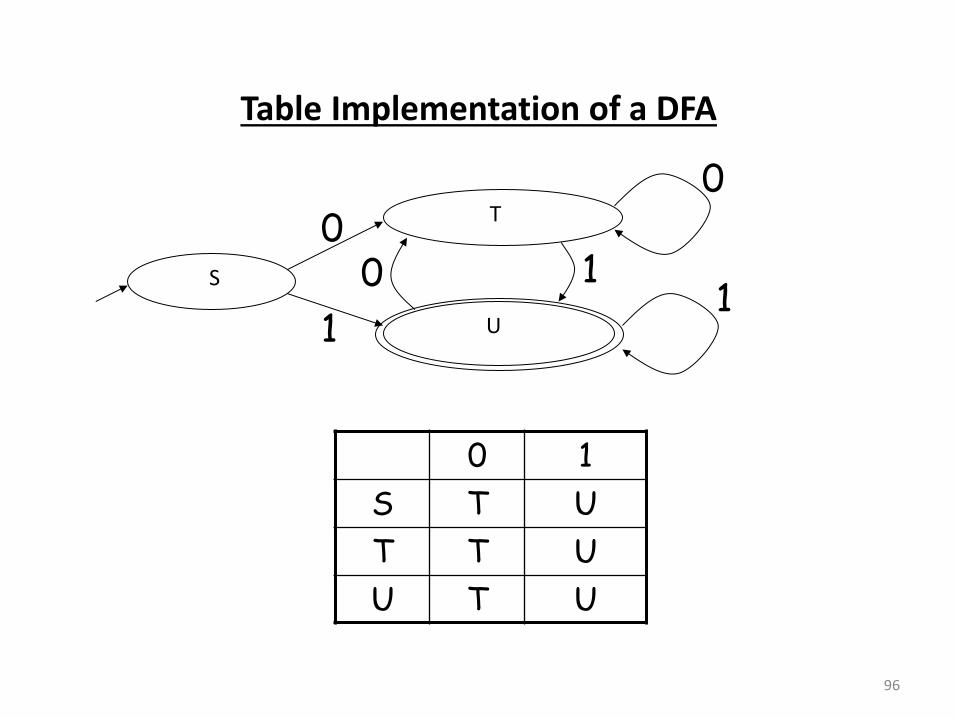
Table Implementation of a DFA

96

S

T

U

0

1

0

1 0 1

0 1

S T U

T T U

U T U

Implementation (Cont.)

• NFA -> DFA conversion is at the heart of tools such as flex or

jflex

• But, DFAs can be huge

• In practice, flex-like tools trade off speed for space in the

choice of NFA and DFA representations

97

UNIT-1

PATR-B

Top Down Parsing

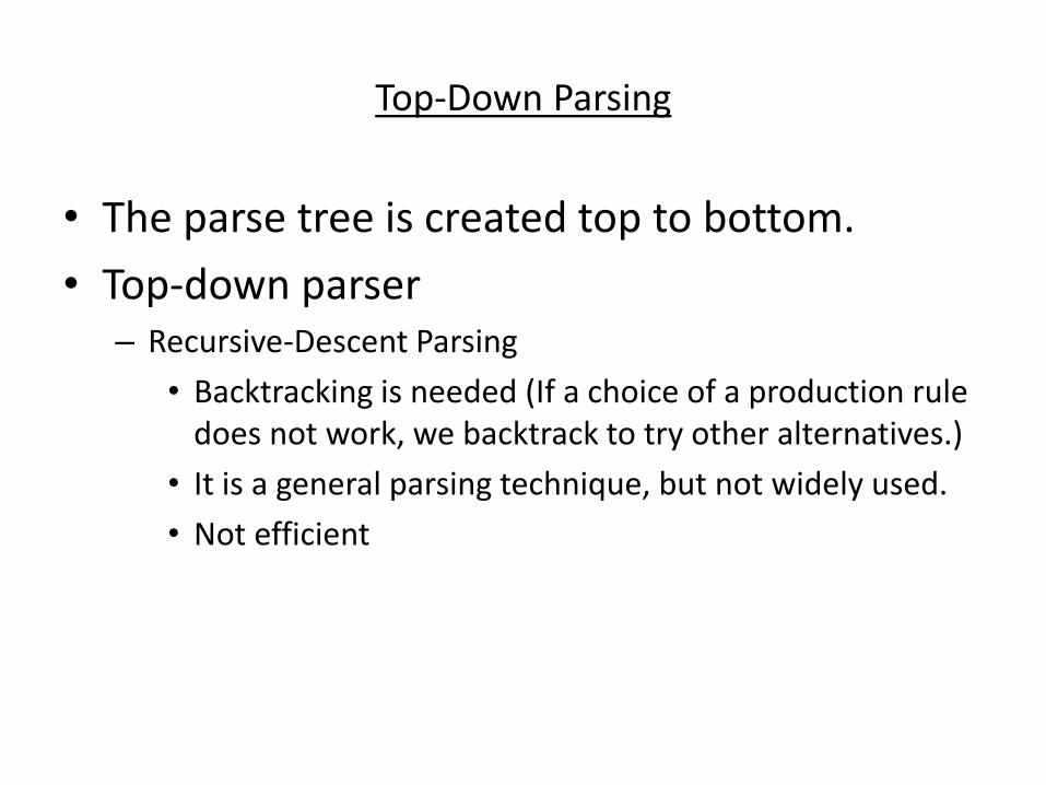
Top-Down Parsing

• The parse tree is created top to bottom.

• Top-down parser – Recursive-Descent Parsing

• Backtracking is needed (If a choice of a production rule

does not work, we backtrack to try other alternatives.)

• It is a general parsing technique, but not widely used.

• Not efficient

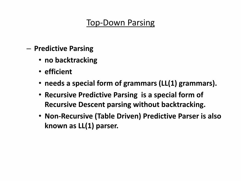
Top-Down Parsing

– Predictive Parsing

• no backtracking

• efficient

• needs a special form of grammars (LL(1) grammars).

• Recursive Predictive Parsing is a special form of

Recursive Descent parsing without backtracking.

• Non-Recursive (Table Driven) Predictive Parser is also

known as LL(1) parser.

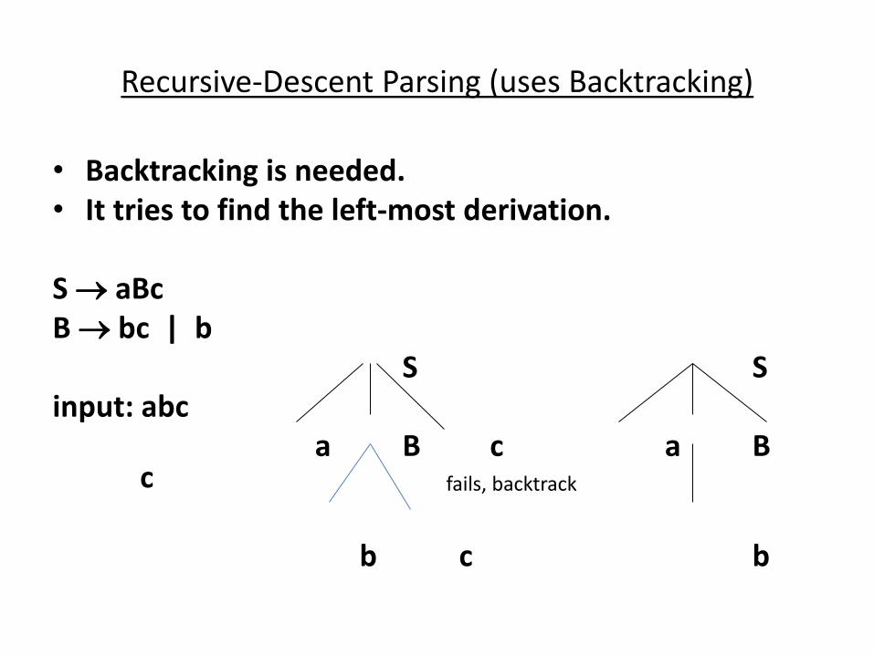
Recursive-Descent Parsing (uses Backtracking)

• Backtracking is needed.

• It tries to find the left-most derivation.

S aBc

B bc | b

S S

input: abc

a B c a B c

b c b

fails, backtrack

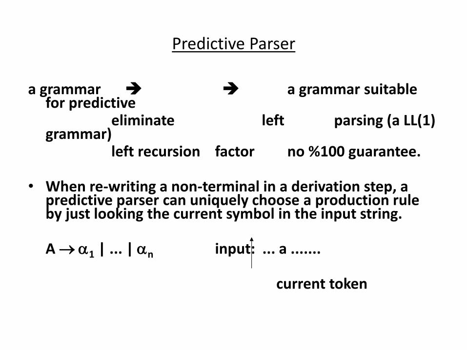
Predictive Parser

a grammar a grammar suitable for predictive

eliminate left parsing (a LL(1) grammar)

left recursion factor no %100 guarantee. • When re-writing a non-terminal in a derivation step, a

predictive parser can uniquely choose a production rule by just looking the current symbol in the input string.

A 1 | ... | n input: ... a ....... current token

Predictive Parser (example)

stmt if ...... |

while ...... |

begin ...... |

for .....

• When we are trying to write the non-terminal stmt, if the current token is if we have to choose first production rule.

• When we are trying to write the non-terminal stmt, we can uniquely choose the production rule by just looking the current token.

• We eliminate the left recursion in the grammar, and left factor it. But it may not be suitable for predictive parsing (not LL(1) grammar).

Recursive Predictive Parsing

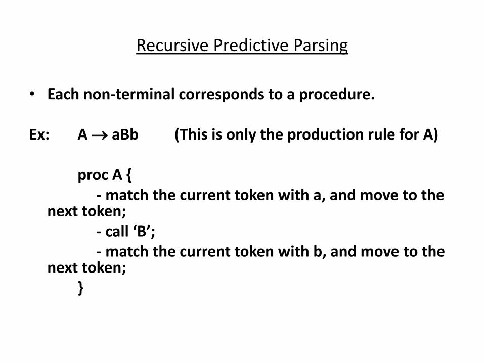
• Each non-terminal corresponds to a procedure.

Ex: A aBb (This is only the production rule for A)

proc A {

- match the current token with a, and move to the next token;

- all B ; - match the current token with b, and move to the

next token;

}

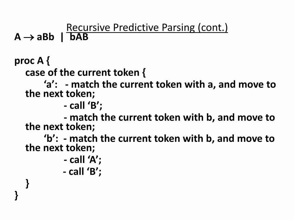
Recursive Predictive Parsing (cont.) A aBb | bAB proc A { case of the current token { a : - match the current token with a, and move to

the next token; - all B ; - match the current token with b, and move to

the next token; : - match the current token with b, and move to

the next token; - all A ; - all B ; } }

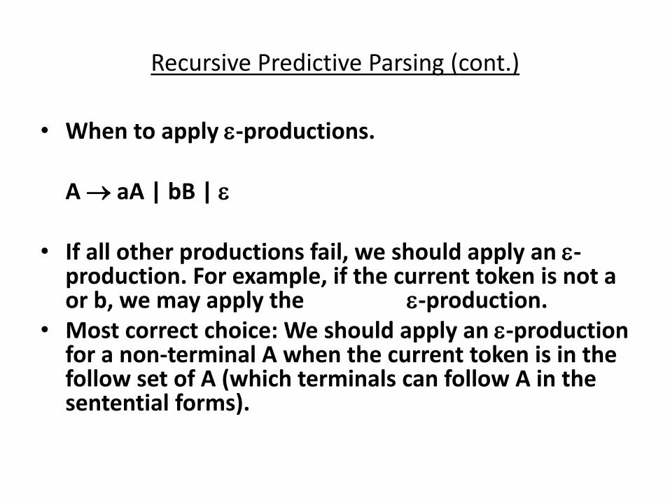
Recursive Predictive Parsing (cont.)

• When to apply -productions.

A aA | bB |

• If all other productions fail, we should apply an -production. For example, if the current token is not a or b, we may apply the -production.

• Most correct choice: We should apply an -production for a non-terminal A when the current token is in the follow set of A (which terminals can follow A in the sentential forms).

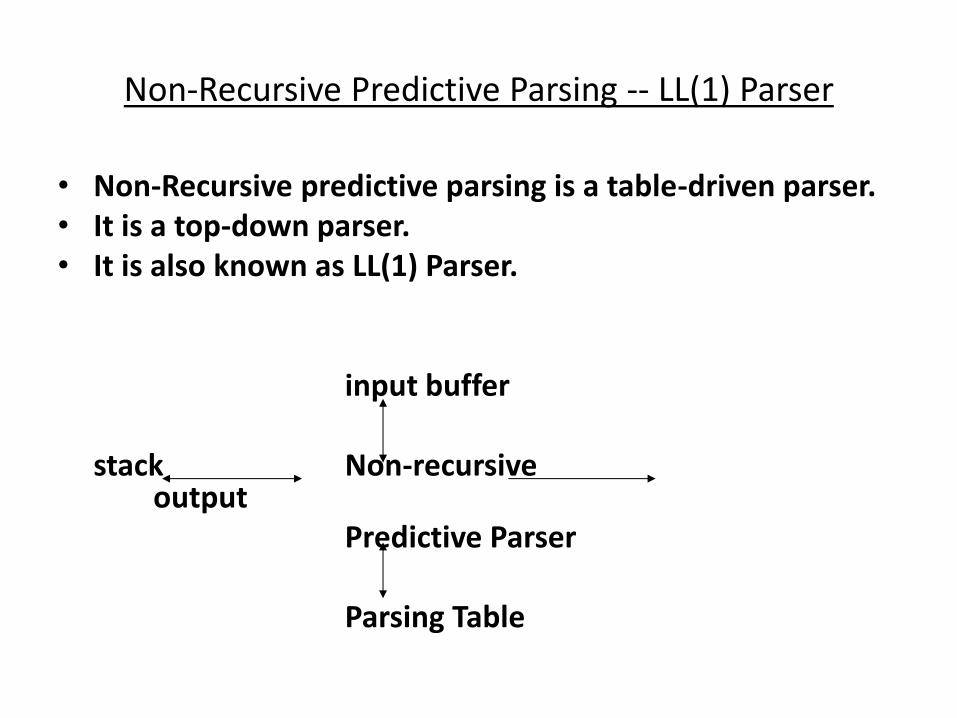
Non-Recursive Predictive Parsing -- LL(1) Parser

• Non-Recursive predictive parsing is a table-driven parser.

• It is a top-down parser.

• It is also known as LL(1) Parser.

input buffer

stack Non-recursive output

Predictive Parser

Parsing Table

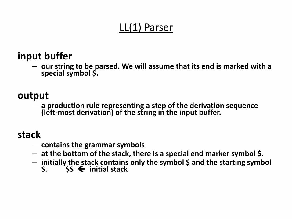
LL(1) Parser input buffer

– our string to be parsed. We will assume that its end is marked with a special symbol $.

output – a production rule representing a step of the derivation sequence

(left-most derivation) of the string in the input buffer.

stack – contains the grammar symbols – at the bottom of the stack, there is a special end marker symbol $. – initially the stack contains only the symbol $ and the starting symbol

S. $S initial stack – when the stack is emptied (ie. only $ left in the stack), the parsing is

completed.

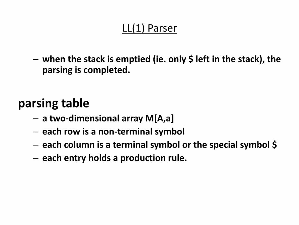
LL(1) Parser

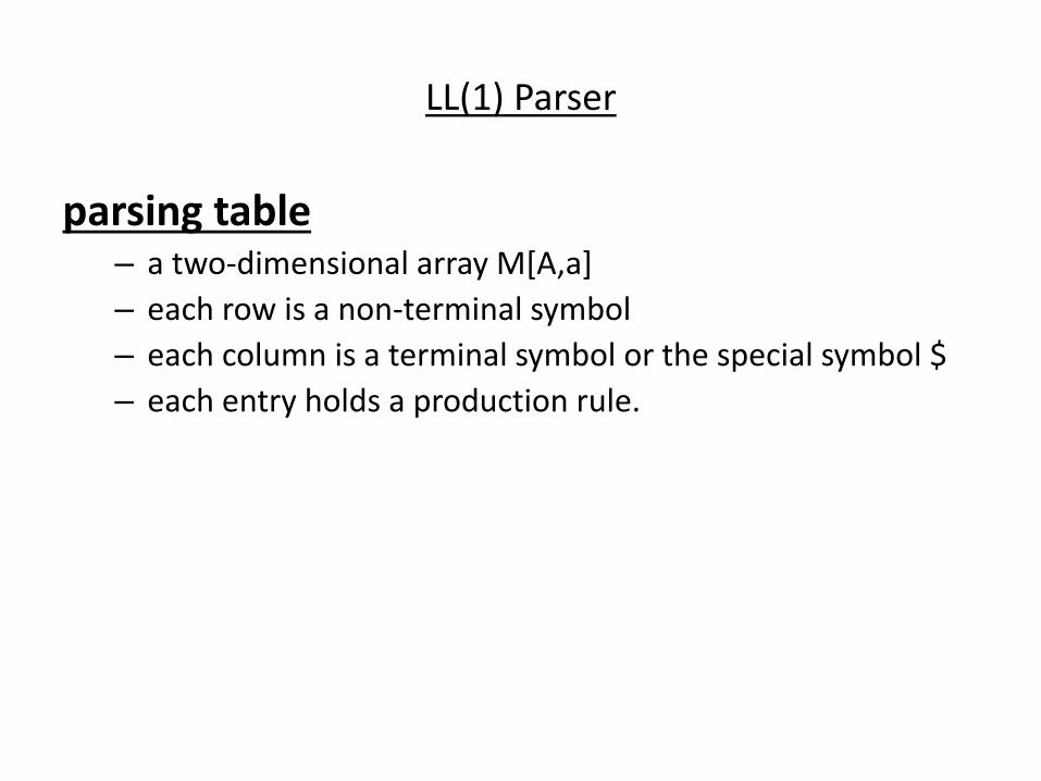
parsing table – a two-dimensional array M[A,a]

– each row is a non-terminal symbol

– each column is a terminal symbol or the special symbol $

– each entry holds a production rule.

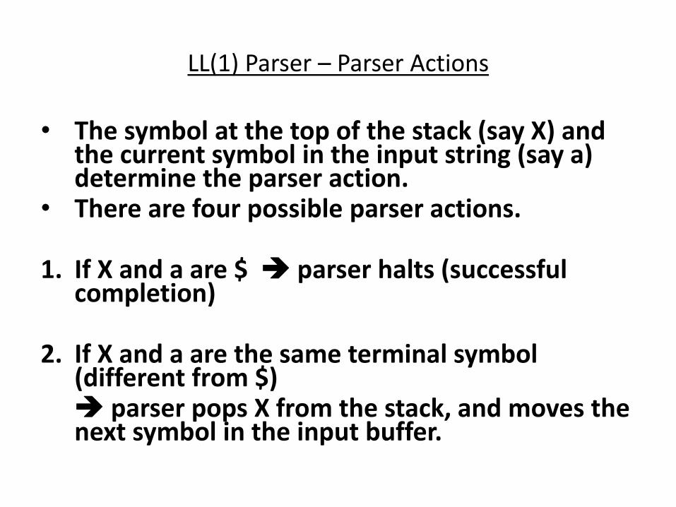
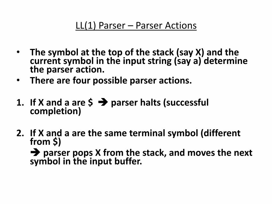
LL(1) Parser – Parser Actions

• The symbol at the top of the stack (say X) and the current symbol in the input string (say a) determine the parser action.

• There are four possible parser actions.

1. If X and a are $ parser halts (successful completion)

2. If X and a are the same terminal symbol (different from $)

parser pops X from the stack, and moves the next symbol in the input buffer.

LL(1) Parser – Parser Actions

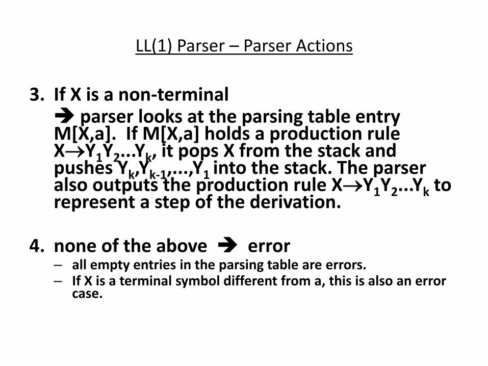
3. If X is a non-terminal parser looks at the parsing table entry

M[X,a]. If M[X,a] holds a production rule XY1Y2...Yk, it pops X from the stack and pushes Yk,Yk-1,...,Y1 into the stack. The parser also outputs the production rule XY1Y2...Yk to represent a step of the derivation.

4. none of the above error

– all empty entries in the parsing table are errors. – If X is a terminal symbol different from a, this is also an error

case.

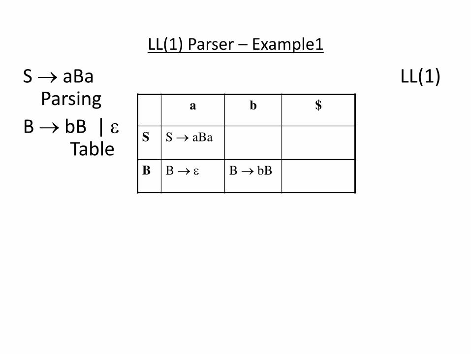
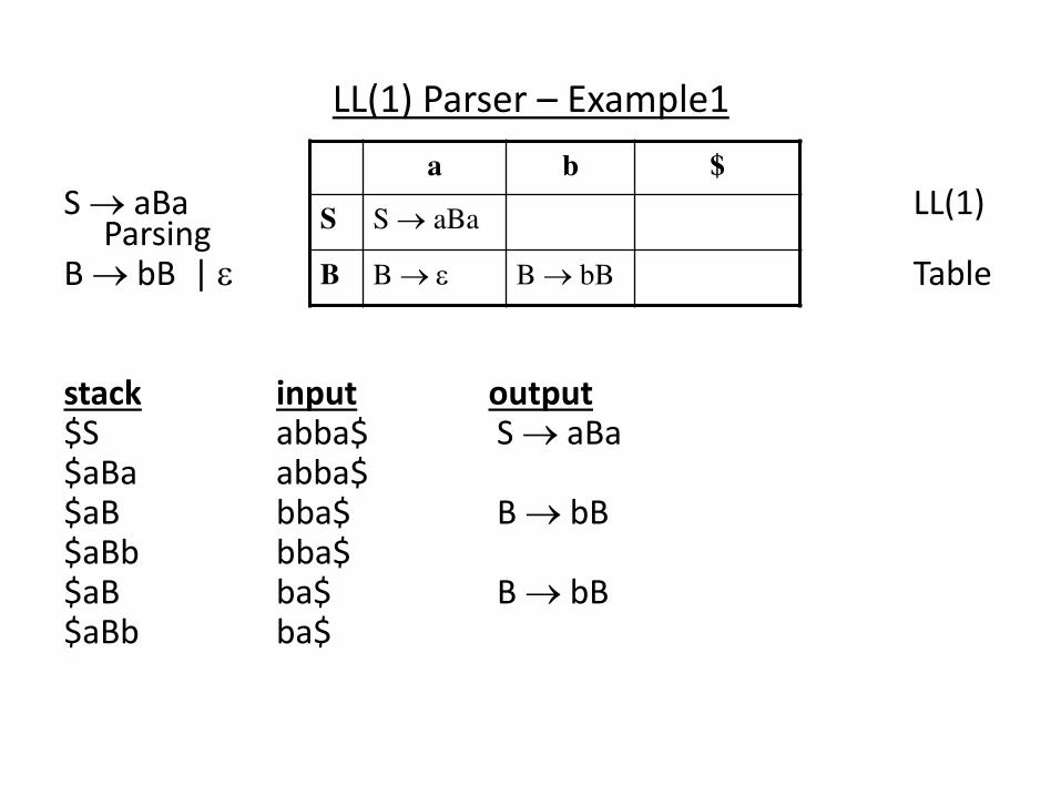
LL(1) Parser – Example1

S aBa LL(1) Parsing

B bB | Table

a b $

S S aBa

B B B bB

LL(1) Parser – Example

stack input output $S abba$ S aBa $aBa abba$ $aB bba$ B bB $aBb bba$ $aB ba$ B bB $aBb ba$ $aB a$ B $a a$ $ $ accept, successful

completion

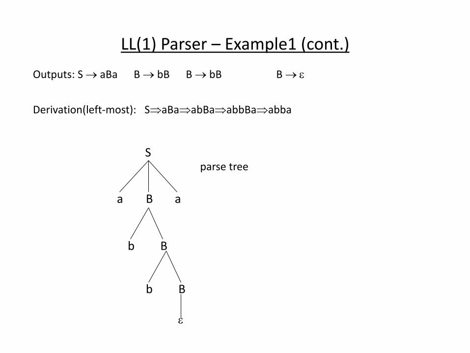
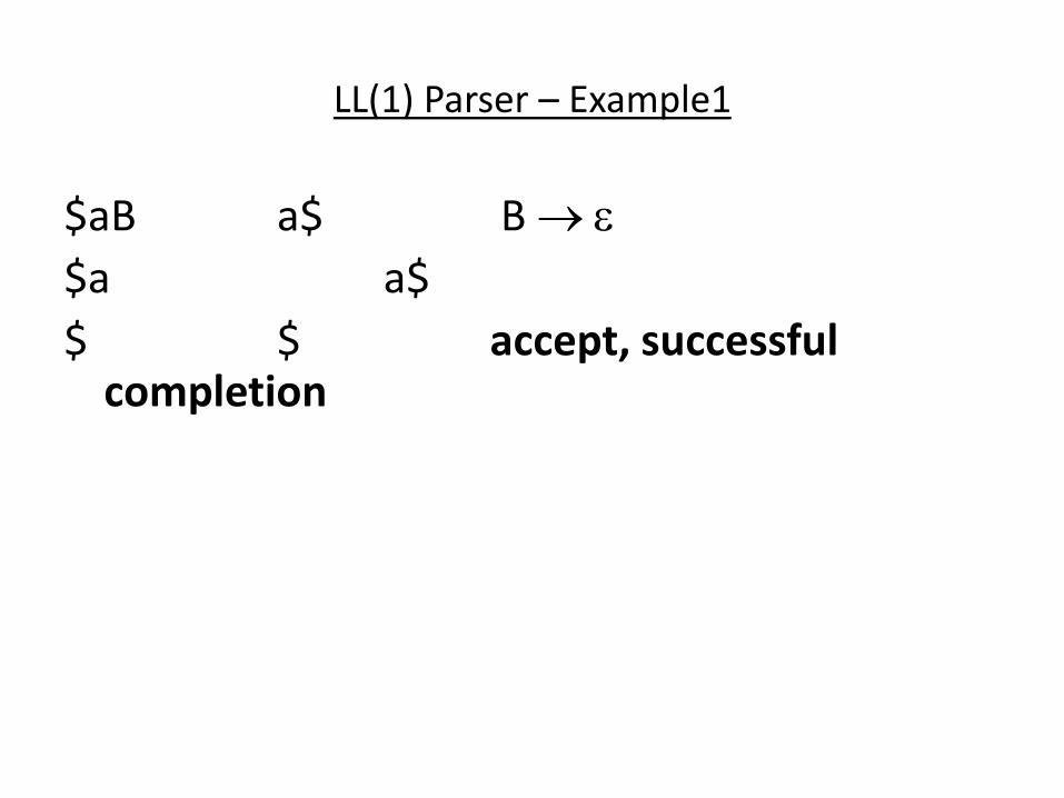
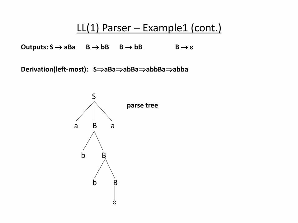
LL(1) Parser – Example1 (cont.)

Outputs: S aBa B bB B bB B

Derivation(left-most): SaBaabBaabbBaabba

S

B a a

B

B b

b

parse tree

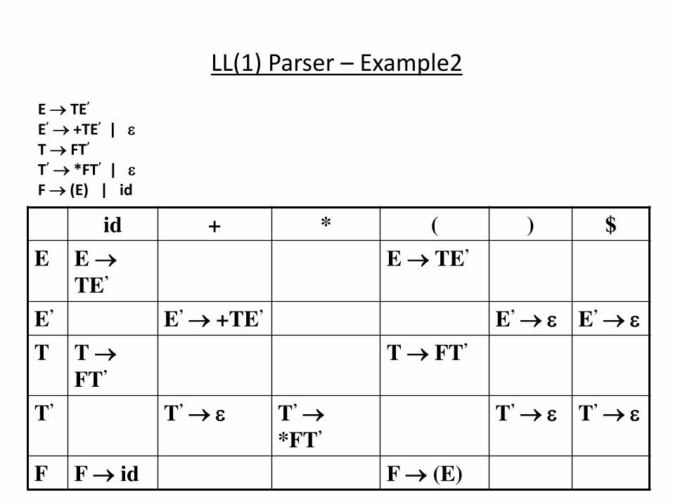
LL(1) Parser – Example2

E TE’

E’ +TE’ |

T FT’

T’ *FT’ |

F (E) | id

id + * ( ) $

E E

TE’ E TE’

E’ E’ +TE’ E’ E’ T T

FT’ T FT’

T’ T’ T’ *FT’ T’ T’ F F id F (E)

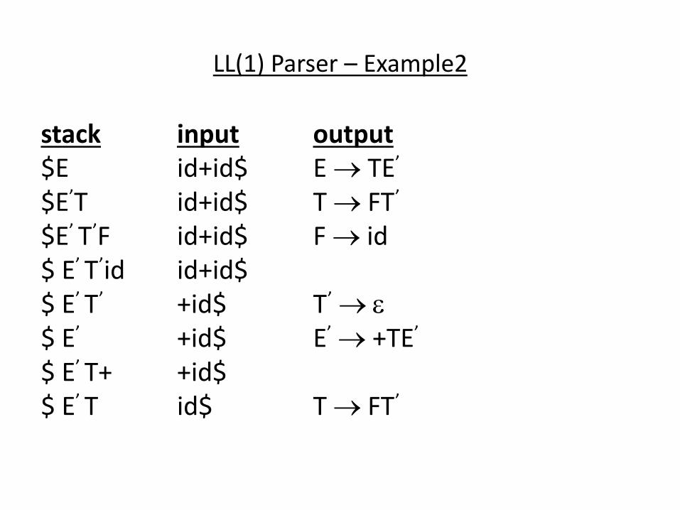
LL(1) Parser – Example2 stack input output

$E id+id$ E TE

$E T id+id$ T FT

$E T F id+id$ F id

$ E T id id+id$

$ E T +id$ T

$ E +id$ E +TE

$ E T+ +id$

$ E T id$ T FT

$ E T F id$ F id

$ E T id id$

$ E T $ T

$ E $ E

$ $ accept

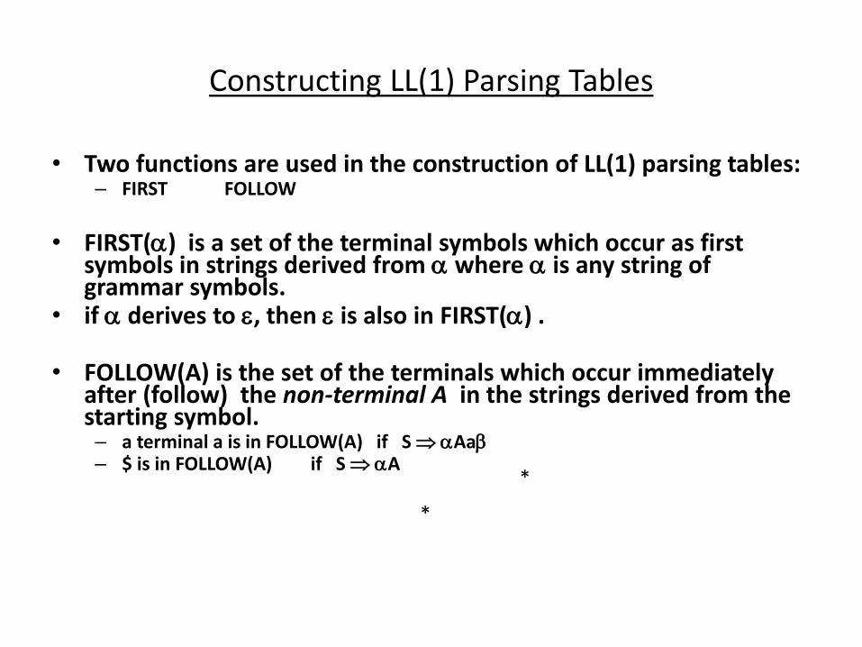
Constructing LL(1) Parsing Tables

• Two functions are used in the construction of LL(1) parsing tables: – FIRST FOLLOW

• FIRST() is a set of the terminal symbols which occur as first

symbols in strings derived from where is any string of grammar symbols.

• if derives to , then is also in FIRST() .

• FOLLOW(A) is the set of the terminals which occur immediately after (follow) the non-terminal A in the strings derived from the starting symbol. – a terminal a is in FOLLOW(A) if S Aa – $ is in FOLLOW(A) if S A

*

*

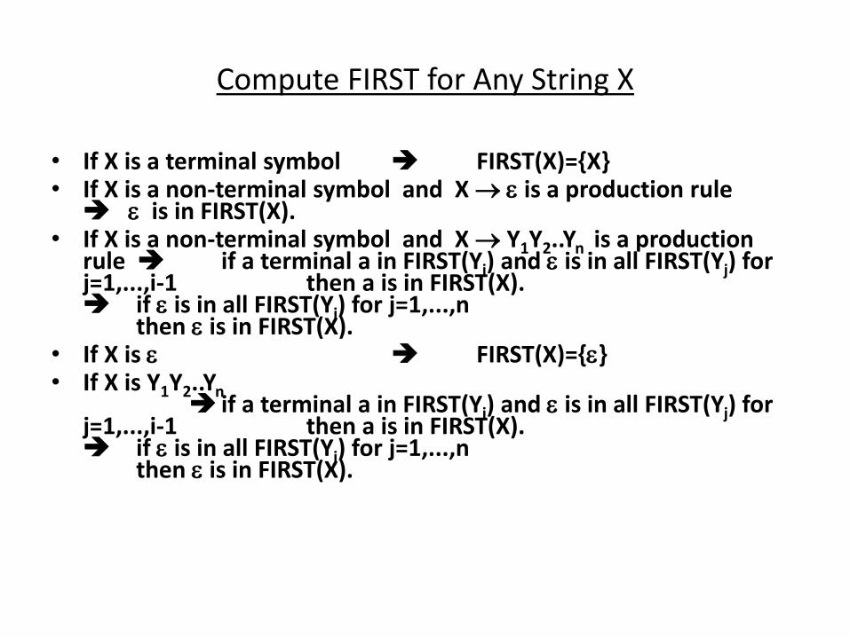
Compute FIRST for Any String X

• If X is a terminal symbol FIRST(X)={X} • If X is a non-terminal symbol and X is a production rule

is in FIRST(X). • If X is a non-terminal symbol and X Y1Y2..Yn is a production

rule if a terminal a in FIRST(Yi) and is in all FIRST(Yj) for j=1,...,i-1 then a is in FIRST(X). if is in all FIRST(Yj) for j=1,...,n then is in FIRST(X).

• If X is FIRST(X)={} • If X is Y1Y2..Yn

if a terminal a in FIRST(Yi) and is in all FIRST(Yj) for j=1,...,i-1 then a is in FIRST(X). if is in all FIRST(Yj) for j=1,...,n then is in FIRST(X).

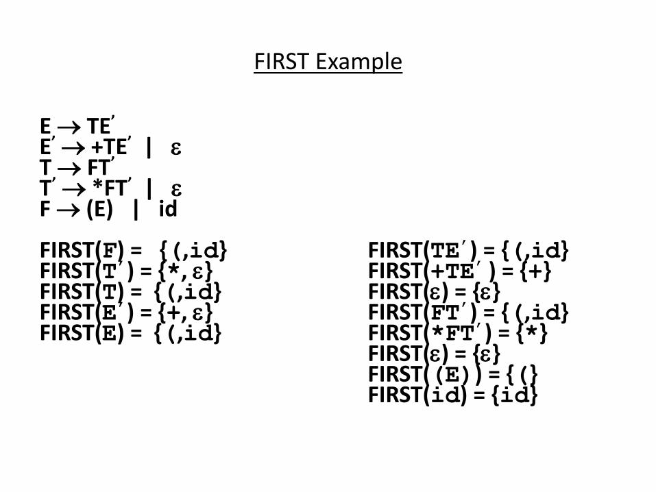
FIRST Example

E TE

E +TE |

T FT

T *FT |

F (E) | id FIRST(F) = {(,id} FIRST(TE’) = {(,id} FIRST(T’) = {*, } FIRST(+TE’ ) = {+} FIRST(T) = {(,id} FIRST() = {} FIRST(E’) = {+, } FIRST(FT’) = {(,id} FIRST(E) = {(,id} FIRST(*FT’) = {*} FIRST() = {} FIRST((E)) = {(} FIRST(id) = {id}

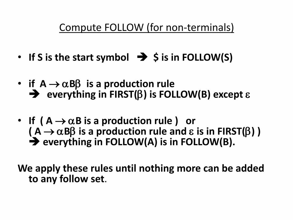
Compute FOLLOW (for non-terminals)

• If S is the start symbol $ is in FOLLOW(S)

• if A B is a production rule everything in FIRST() is FOLLOW(B) except

• If ( A B is a production rule ) or ( A B is a production rule and is in FIRST() ) everything in FOLLOW(A) is in FOLLOW(B).

We apply these rules until nothing more can be added to any follow set.

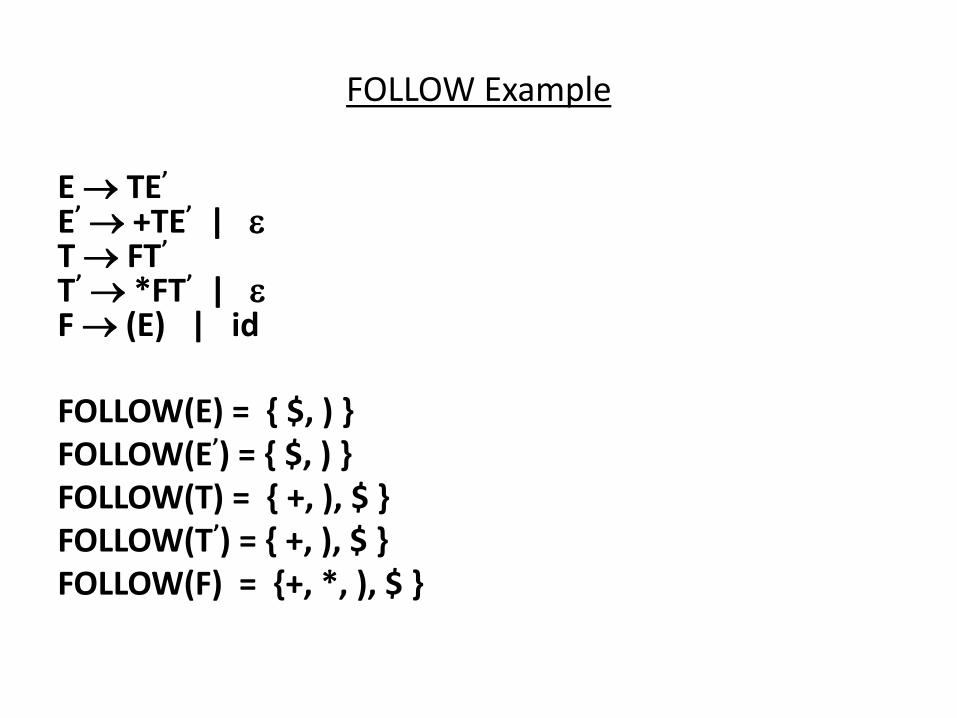
FOLLOW Example

E TE

E +TE |

T FT

T *FT |

F (E) | id

FOLLOW(E) = { $, ) }

FOLLOW(E ) = { $, ) }

FOLLOW(T) = { +, ), $ }

FOLLOW(T ) = { +, ), $ }

FOLLOW(F) = {+, *, ), $ }

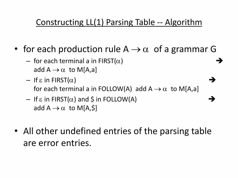
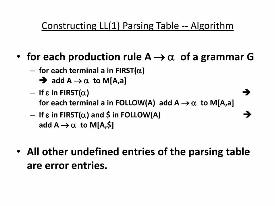
Constructing LL(1) Parsing Table -- Algorithm

• for each production rule A of a grammar G – for each terminal a in FIRST()

add A to M[A,a]

– If in FIRST()

for each terminal a in FOLLOW(A) add A to M[A,a]

– If in FIRST() and $ in FOLLOW(A)

add A to M[A,$]

• All other undefined entries of the parsing table

are error entries.

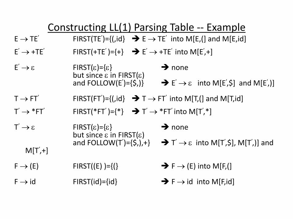
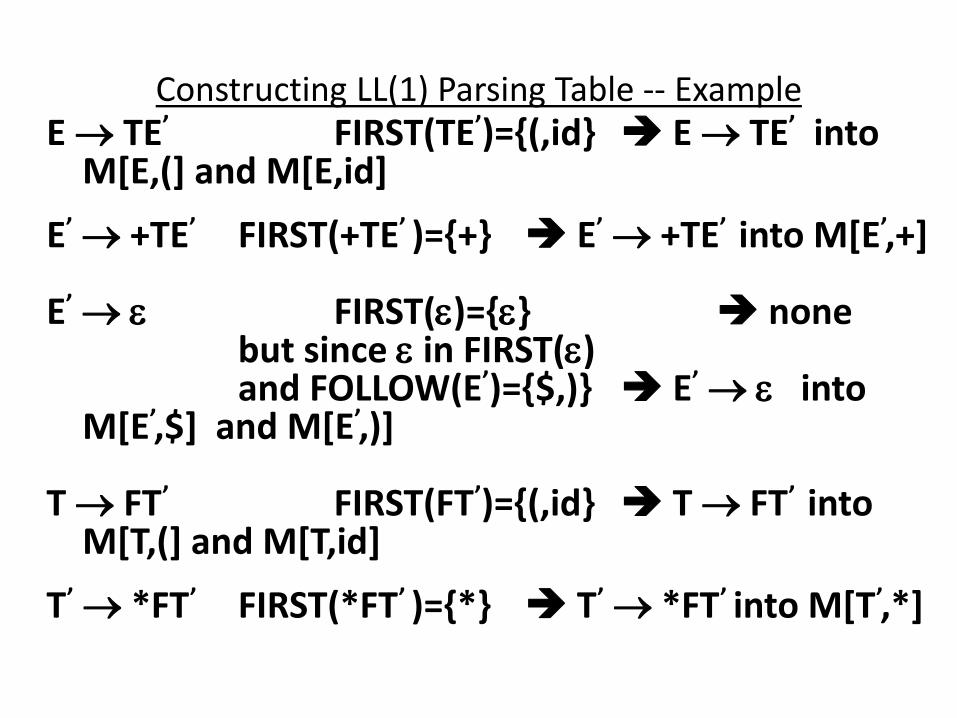
Constructing LL(1) Parsing Table -- Example E TE’ FIRST(TE’)={(,id} E TE’ into M[E,(] and M[E,id]

E’ +TE’ FIRST(+TE’ )={+} E’ +TE’ into M[E’,+]

E’ FIRST()={} none but since in FIRST() and FOLLOW(E’)={$,)} E’ into M[E’,$] and M[E’,)] T FT’ FIRST(FT’)={(,id} T FT’ into M[T,(] and M[T,id]

T’ *FT’ FIRST(*FT’ )={*} T’ *FT’ into M[T’,*]

T’ FIRST()={} none but since in FIRST() and FOLLOW(T’)={$,),+} T’ into M[T’,$], M[T’,)] and

M[T’,+] F (E) FIRST((E) )={(} F (E) into M[F,(] F id FIRST(id)={id} F id into M[F,id]

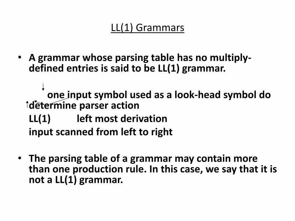
LL(1) Grammars

• A grammar whose parsing table has no multiply-defined entries is said to be LL(1) grammar.

one input symbol used as a look-head symbol do determine parser action

LL(1) left most derivation

input scanned from left to right

• The parsing table of a grammar may contain more than one production rule. In this case, we say that it is not a LL(1) grammar.

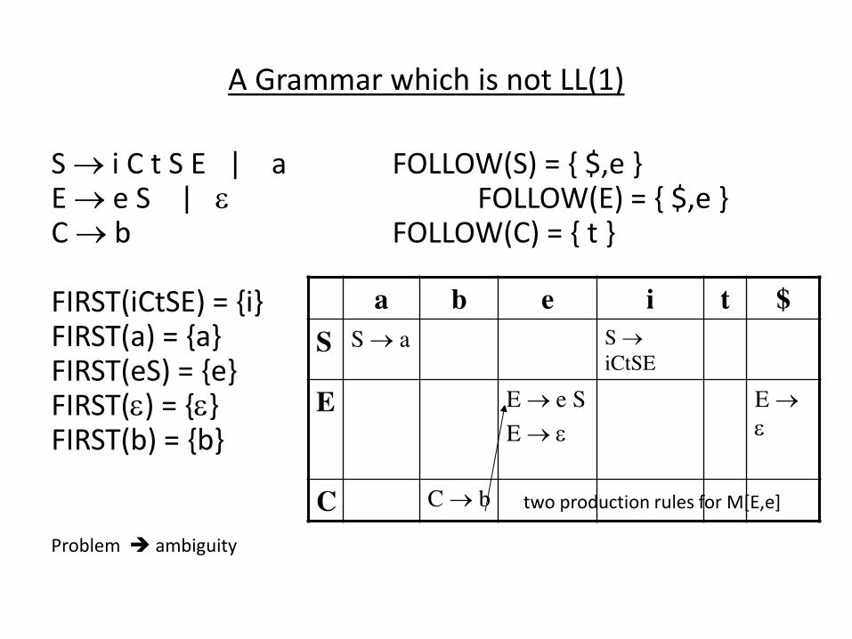
A Grammar which is not LL(1)

S i C t S E | a FOLLOW(S) = { $,e } E e S | FOLLOW(E) = { $,e } C b FOLLOW(C) = { t } FIRST(iCtSE) = {i} FIRST(a) = {a} FIRST(eS) = {e} FIRST() = {} FIRST(b) = {b} two production rules for M[E,e] Problem ambiguity

a b e i t $

S S a S

iCtSE

E E e S

E E

C C b

A Grammar which is not LL(1) (cont.)

• What do we have to do it if the resulting

parsing table contains multiply defined

entries? – If we did ’t eli i ate left re ursio , eli i ate the left

recursion in the grammar.

– If the grammar is not left factored, we have to left factor

the grammar.

– If its ew gra ar’s parsi g ta le still o tai s ultiply defined entries, that grammar is ambiguous or it is

inherently not a LL(1) grammar.

A Grammar which is not LL(1) (cont.)

• A left recursive grammar cannot be a LL(1) grammar. – A A |

any terminal that appears in FIRST() also appears FIRST(A) because A .

If is , any terminal that appears in FIRST() also appears in FIRST(A) and FOLLOW(A).

• A grammar is not left factored, it cannot be a LL(1) grammar • A 1 | 2

any terminal that appears in FIRST(1) also appears in FIRST(2).

• An ambiguous grammar cannot be a LL(1) grammar.

Properties of LL(1) Grammars

• A grammar G is LL(1) if and only if the following conditions hold for two distinctive production rules A and A

1. Both and cannot derive strings starting with same

terminals.

2. At most one of and can derive to .

3. If can derive to , then cannot derive to any string starting with a terminal in FOLLOW(A).

Error Recovery in Predictive Parsing

• An error may occur in the predictive parsing

(LL(1) parsing) – if the terminal symbol on the top of stack does not match with

the current input symbol.

– if the top of stack is a non-terminal A, the current input symbol

is a, and the parsing table entry M[A,a] is empty.

• What should the parser do in an error case? – The parser should be able to give an error message (as much

as possible meaningful error message).

– It should be recover from that error case, and it should be able

to continue the parsing with the rest of the input.

Error Recovery Techniques

• Panic-Mode Error Recovery – Skipping the input symbols until a synchronizing token is

found.

• Phrase-Level Error Recovery – Each empty entry in the parsing table is filled with a pointer to

a specific error routine to take care that error case.

• Error-Productions – If we have a good idea of the common errors that might be

encountered, we can augment the grammar with productions that generate erroneous constructs.

– When an error production is used by the parser, we can generate appropriate error diagnostics.

– Since it is almost impossible to know all the errors that can be made by the programmers, this method is not practical.

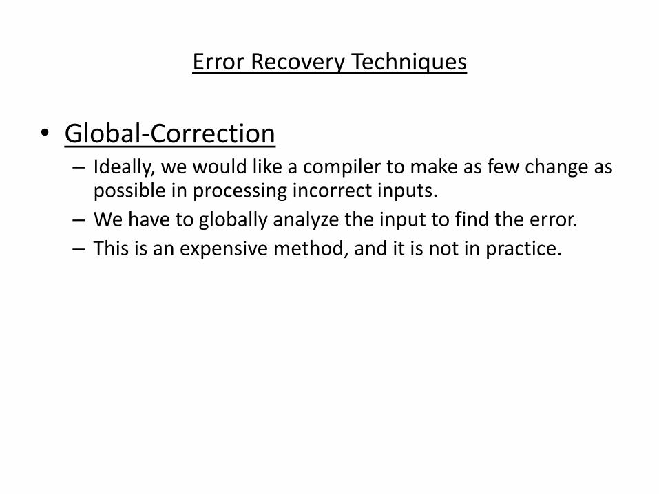
Error Recovery Techniques

• Global-Correction – Ideally, we would like a compiler to make as few change as

possible in processing incorrect inputs.

– We have to globally analyze the input to find the error.

– This is an expensive method, and it is not in practice.

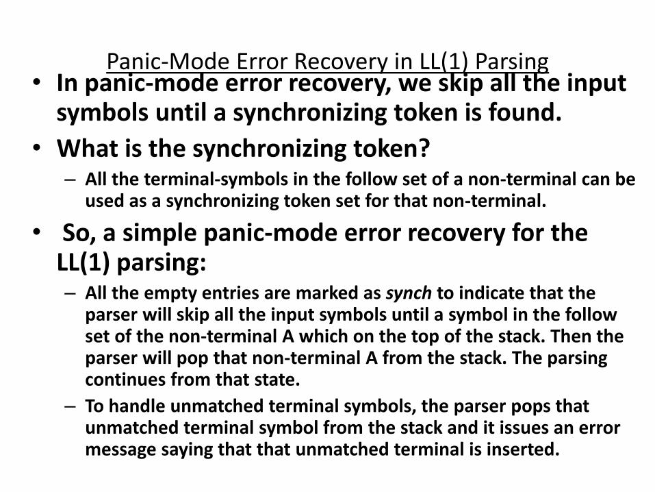
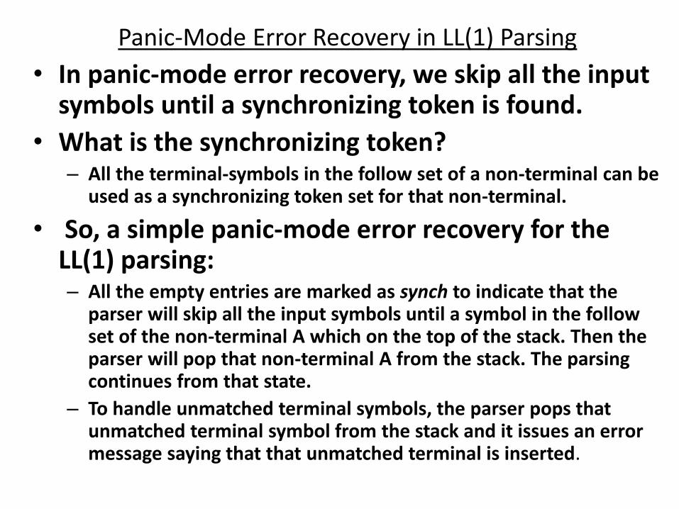
Panic-Mode Error Recovery in LL(1) Parsing • In panic-mode error recovery, we skip all the input

symbols until a synchronizing token is found.

• What is the synchronizing token? – All the terminal-symbols in the follow set of a non-terminal can be

used as a synchronizing token set for that non-terminal.

• So, a simple panic-mode error recovery for the LL(1) parsing: – All the empty entries are marked as synch to indicate that the

parser will skip all the input symbols until a symbol in the follow set of the non-terminal A which on the top of the stack. Then the parser will pop that non-terminal A from the stack. The parsing continues from that state.

– To handle unmatched terminal symbols, the parser pops that unmatched terminal symbol from the stack and it issues an error message saying that that unmatched terminal is inserted.

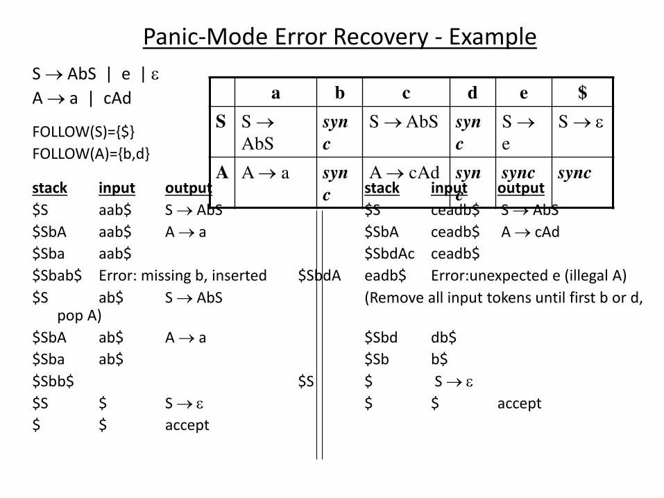
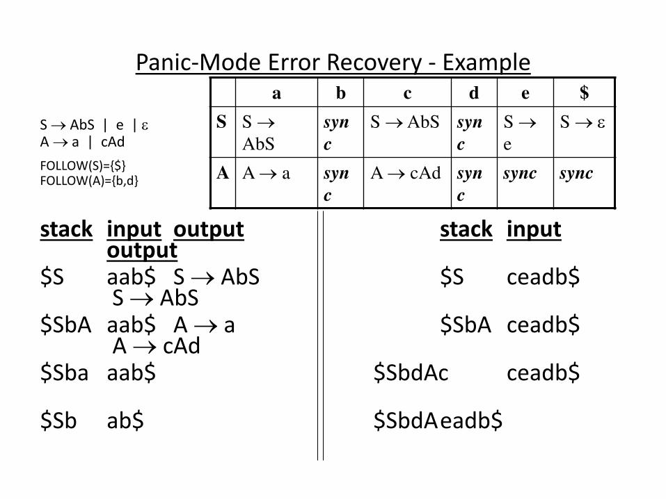
Panic-Mode Error Recovery - Example

S AbS | e |

A a | cAd

FOLLOW(S)={$}

FOLLOW(A)={b,d}

stack input output stack input output

$S aab$ S AbS $S ceadb$ S AbS

$SbA aab$ A a $SbA ceadb$ A cAd

$Sba aab$ $SbdAc ceadb$

$Sb ab$ Error: missing b, inserted $SbdA eadb$ Error:unexpected e (illegal A)

$S ab$ S AbS (Remove all input tokens until first b or d, pop A)

$SbA ab$ A a $Sbd db$

$Sba ab$ $Sb b$

$Sb b$ $S $ S

$S $ S $ $ accept

$ $ accept

a b c d e $

S S

AbS

syn

c

S AbS syn

c

S

e

S

A A a syn

c

A cAd syn

c

sync sync

Phrase-Level Error Recovery

• Each empty entry in the parsing table is filled with a pointer to a special error routine which will take care that error case.

• These error routines may: – change, insert, or delete input symbols.

– issue appropriate error messages

– pop items from the stack.

• We should be careful when we design these error routines, because we may put the parser into an infinite loop.

Syntax Analyzer

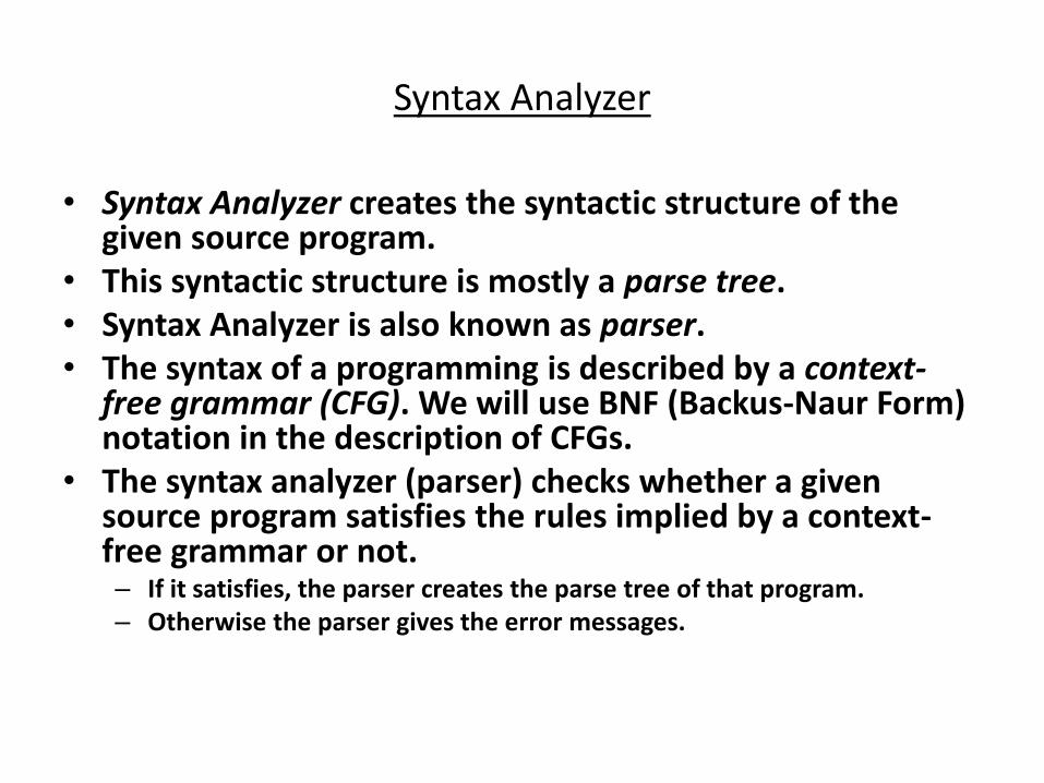
• Syntax Analyzer creates the syntactic structure of the given source program.

• This syntactic structure is mostly a parse tree.

• Syntax Analyzer is also known as parser.

• The syntax of a programming is described by a context-free grammar (CFG). We will use BNF (Backus-Naur Form) notation in the description of CFGs.

• The syntax analyzer (parser) checks whether a given source program satisfies the rules implied by a context-free grammar or not. – If it satisfies, the parser creates the parse tree of that program.

– Otherwise the parser gives the error messages.

Syntax Analyzer

• A context-free grammar – gives a precise syntactic specification of a programming

language.

– the design of the grammar is an initial phase of the

design of a compiler.

– a grammar can be directly converted into a parser by

some tools.

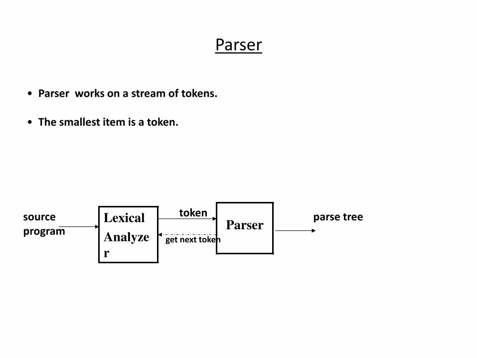
Parser

Lexical

Analyze

r

Parser

source

program

token

get next token

parse tree

• Parser works on a stream of tokens.

• The smallest item is a token.

Parsers (cont.)

• We categorize the parsers into two groups:

1. Top-Down Parser – the parse tree is created top to bottom, starting from the root.

2. Bottom-Up Parser – the parse is created bottom to top; starting from the leaves

• Both top-down and bottom-up parsers scan the input from left to right (one symbol at a time).

• Efficient top-down and bottom-up parsers can be implemented only for sub-classes of context-free grammars. – LL for top-down parsing

– LR for bottom-up parsing

Context-Free Grammars

• Inherently recursive structures of a programming language are defined by a context-free grammar.

• In a context-free grammar, we have: – A finite set of terminals (in our case, this will be the set of

tokens) – A finite set of non-terminals (syntactic-variables) – A finite set of productions rules in the following form

• A where A is a non-terminal and is a string of terminals and non-terminals

(including the empty string) – A start symbol (one of the non-terminal symbol)

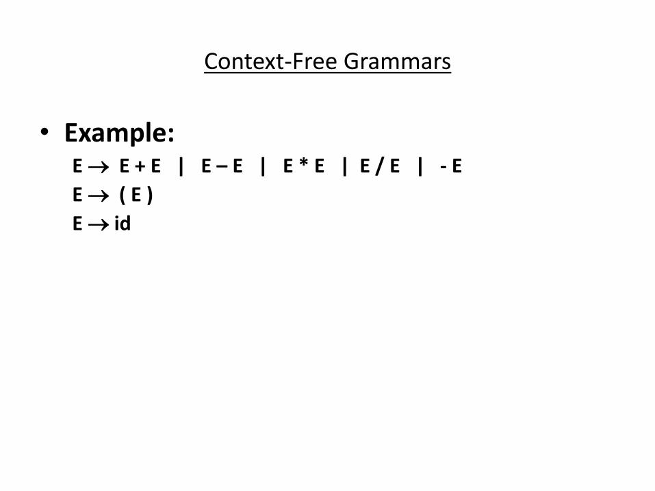
Context-Free Grammars

• Example: E E + E | E – E | E * E | E / E | - E

E ( E )

E id

Derivations

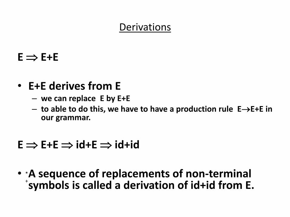
E E+E

• E+E derives from E – we can replace E by E+E

– to able to do this, we have to have a production rule EE+E in our grammar.

E E+E id+E id+id

• A sequence of replacements of non-terminal symbols is called a derivation of id+id from E.

*

+

Derivations

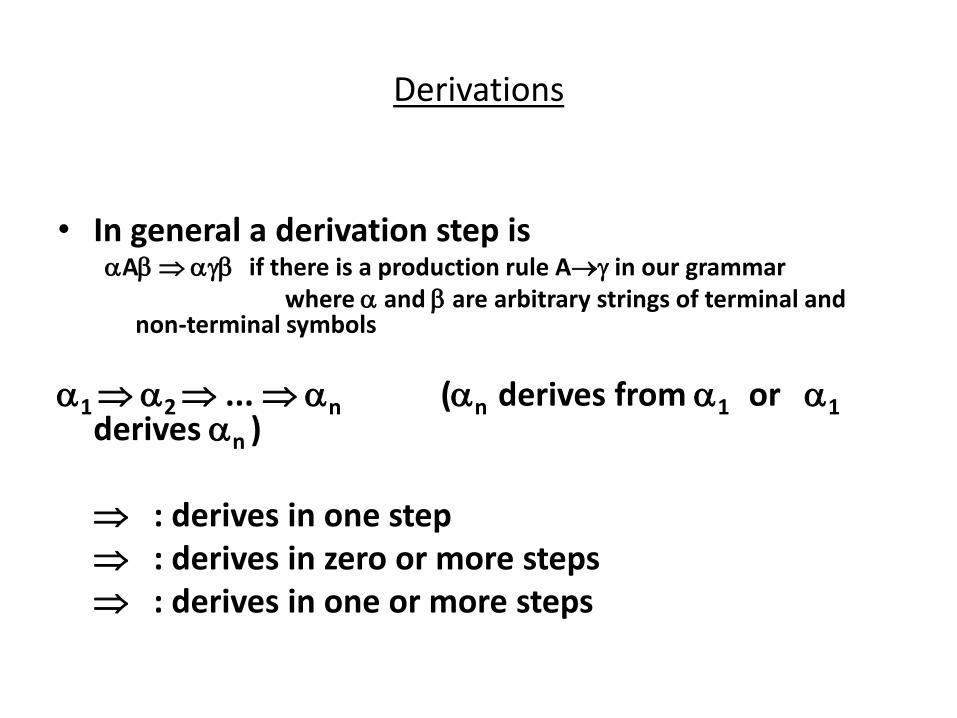
• In general a derivation step is A if there is a production rule A in our grammar

where and are arbitrary strings of terminal and non-terminal symbols

1 2 ... n (n derives from 1 or 1 derives n )

: derives in one step

: derives in zero or more steps

: derives in one or more steps

CFG - Terminology

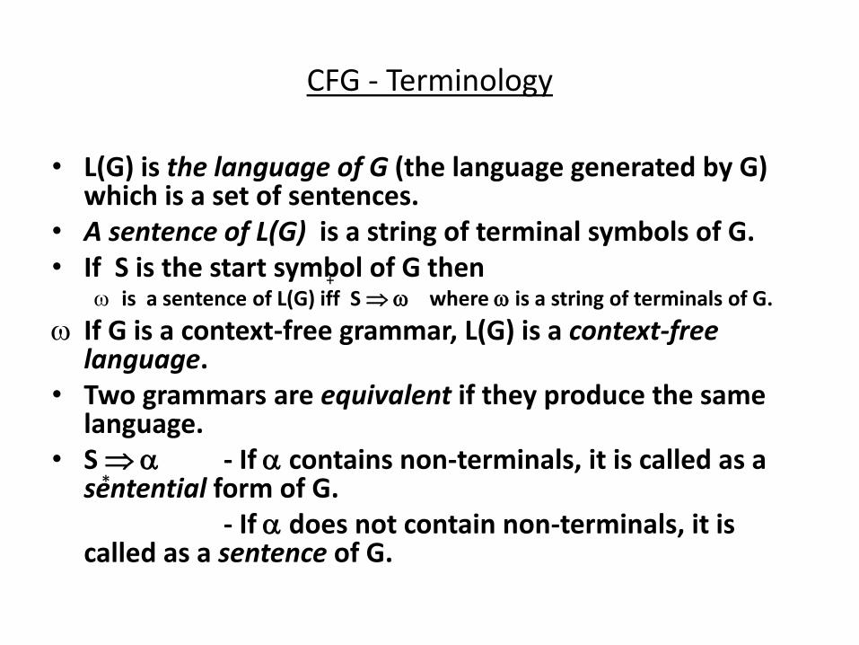
• L(G) is the language of G (the language generated by G) which is a set of sentences.

• A sentence of L(G) is a string of terminal symbols of G.

• If S is the start symbol of G then is a sentence of L(G) iff S where is a string of terminals of G.

If G is a context-free grammar, L(G) is a context-free language.

• Two grammars are equivalent if they produce the same language.

• S - If contains non-terminals, it is called as a sentential form of G.

- If does not contain non-terminals, it is called as a sentence of G.

+

*

Derivation Example

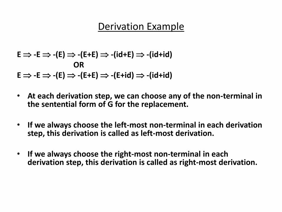
E -E -(E) -(E+E) -(id+E) -(id+id)

OR

E -E -(E) -(E+E) -(E+id) -(id+id)

• At each derivation step, we can choose any of the non-terminal in the sentential form of G for the replacement.

• If we always choose the left-most non-terminal in each derivation step, this derivation is called as left-most derivation.

• If we always choose the right-most non-terminal in each derivation step, this derivation is called as right-most derivation.

Left-Most and Right-Most Derivations

Left-Most Derivation

E -E -(E) -(E+E) -(id+E) -(id+id)

Right-Most Derivation

E -E -(E) -(E+E) -(E+id) -(id+id)

• We will see that the top-down parsers try to find the left-most derivation of the given source program.

• We will see that the bottom-up parsers try to find the right-most derivation of the given source program in the reverse order.

lm lm lm lm lm

rm rm rm rm rm

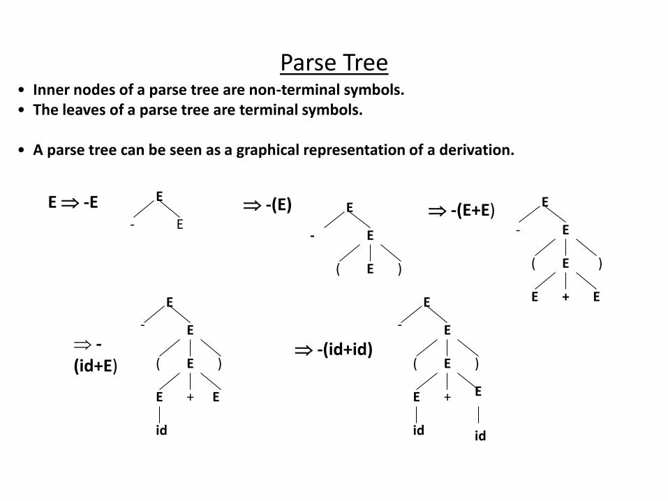
Parse Tree • Inner nodes of a parse tree are non-terminal symbols.

• The leaves of a parse tree are terminal symbols.

• A parse tree can be seen as a graphical representation of a derivation.

E -E E

E -

E

E

E E

E

+

-

( )

E

E

E -

( )

E

E

id

E

E

E +

-

( )

id

E

E

E

E E +

-

( )

id

-(E) -(E+E)

-

(id+E) -(id+id)

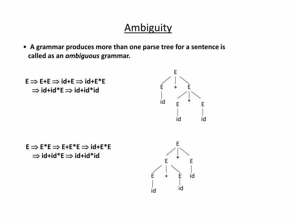
Ambiguity

• A grammar produces more than one parse tree for a sentence is

called as an ambiguous grammar.

E E+E id+E id+E*E

id+id*E id+id*id

E E*E E+E*E id+E*E

id+id*E id+id*id

E

id

E +

id

id

E

E

* E

E

E +

id E

E

* E

id id

Ambiguity (cont.)

• For the most parsers, the grammar must be unambiguous.

• unambiguous grammar

unique selection of the parse tree for a sentence

• We should eliminate the ambiguity in the grammar during the design phase of the compiler.

• An unambiguous grammar should be written to eliminate the ambiguity.

• We have to prefer one of the parse trees of a sentence (generated by an ambiguous grammar) to disambiguate that grammar to restrict to this choice.

Ambiguity (cont.)

stmt if expr then stmt |

if expr then stmt else stmt | otherstmts

if E1 then if E2 then S1 else S2

stmt

if expr then stmt else stmt

E1 if expr then stmt S2

E2 S1

stmt

if expr then stmt

E1 if expr then stmt else stmt

E2 S1 S2

1 2

Ambiguity

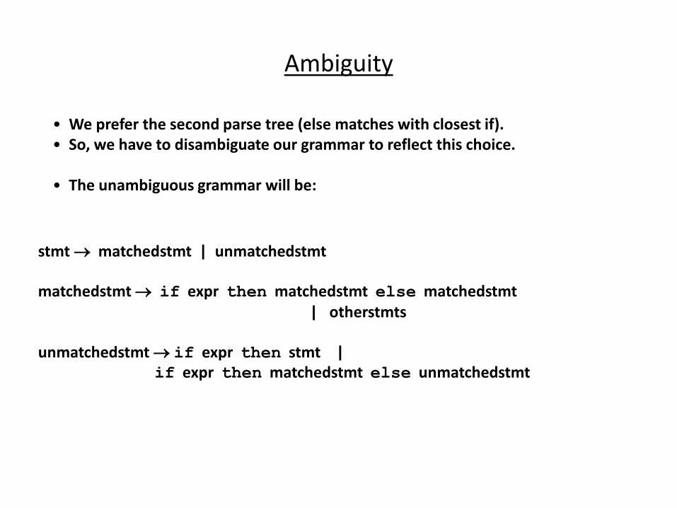
• We prefer the second parse tree (else matches with closest if).

• So, we have to disambiguate our grammar to reflect this choice.

• The unambiguous grammar will be:

stmt matchedstmt | unmatchedstmt

matchedstmt if expr then matchedstmt else matchedstmt

| otherstmts

unmatchedstmt if expr then stmt |

if expr then matchedstmt else unmatchedstmt

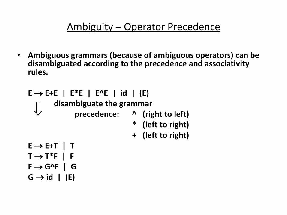
Ambiguity – Operator Precedence

• Ambiguous grammars (because of ambiguous operators) can be disambiguated according to the precedence and associativity rules.

E E+E | E*E | E^E | id | (E)

disambiguate the grammar

precedence: ^ (right to left)

* (left to right)

+ (left to right)

E E+T | T

T T*F | F

F G^F | G

G id | (E)

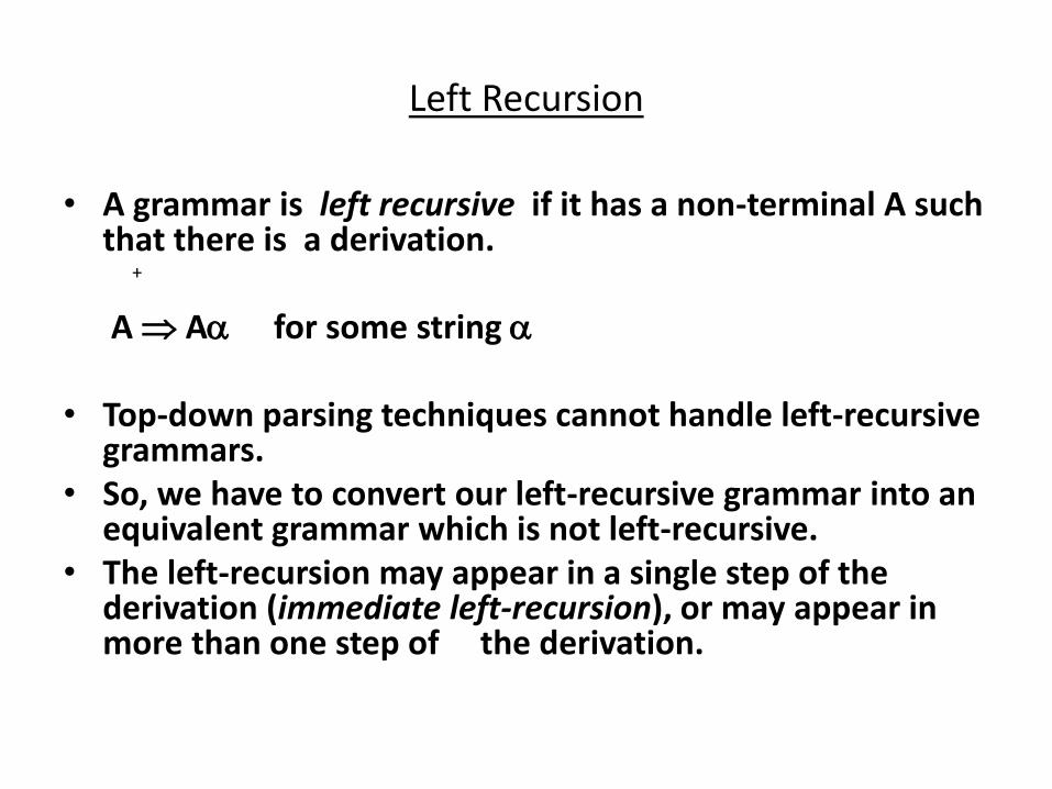
Left Recursion

• A grammar is left recursive if it has a non-terminal A such that there is a derivation.

A A for some string

• Top-down parsing techniques cannot handle left-recursive grammars.

• So, we have to convert our left-recursive grammar into an equivalent grammar which is not left-recursive.

• The left-recursion may appear in a single step of the derivation (immediate left-recursion), or may appear in more than one step of the derivation.

+

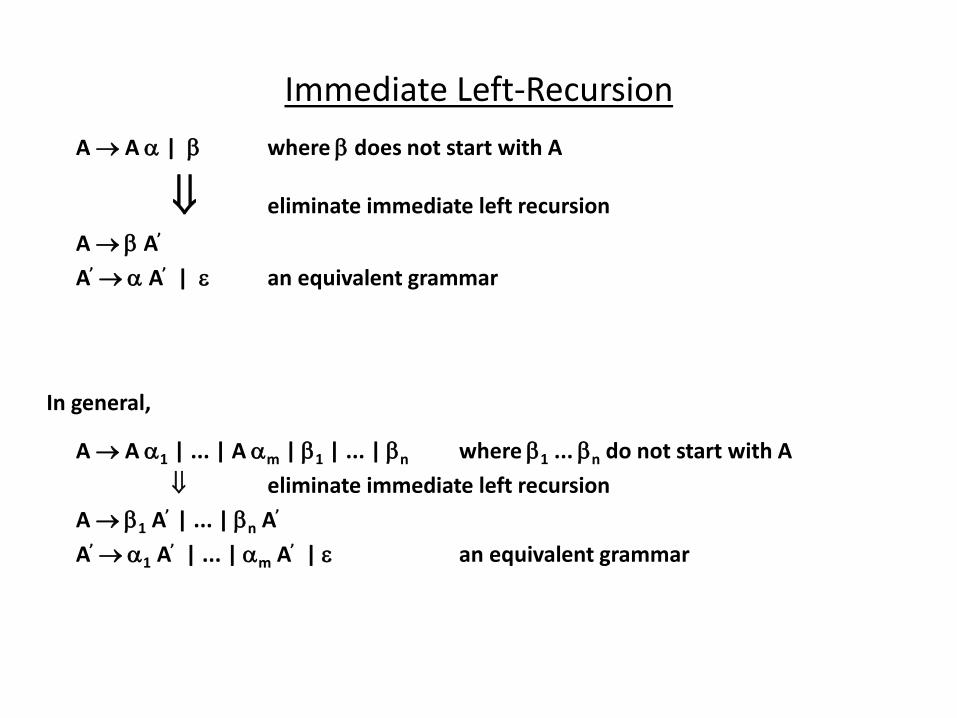
Immediate Left-Recursion

A A | where does not start with A

eliminate immediate left recursion

A A

A A | an equivalent grammar

A A 1 | ... | A m | 1 | ... | n where 1 ... n do not start with A

eliminate immediate left recursion

A 1 A | ... | n A

A 1 A | ... | m A | an equivalent grammar

In general,

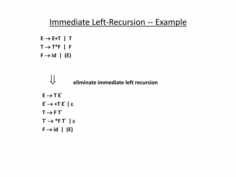
Immediate Left-Recursion -- Example

E E+T | T

T T*F | F

F id | (E)

E T E

E +T E |

T F T

T *F T |

F id | (E)

eliminate immediate left recursion

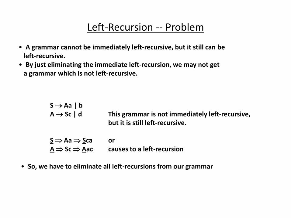
Left-Recursion -- Problem

• A grammar cannot be immediately left-recursive, but it still can be

left-recursive.

• By just eliminating the immediate left-recursion, we may not get

a grammar which is not left-recursive.

S Aa | b

A Sc | d This grammar is not immediately left-recursive,

but it is still left-recursive.

S Aa Sca or

A Sc Aac causes to a left-recursion

• So, we have to eliminate all left-recursions from our grammar

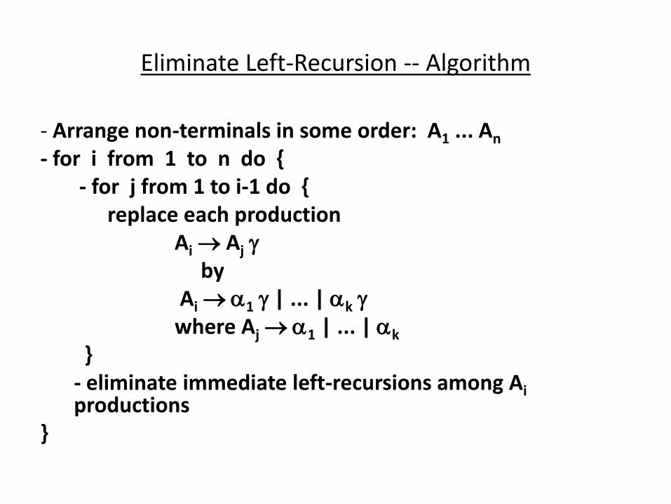
Eliminate Left-Recursion -- Algorithm

- Arrange non-terminals in some order: A1 ... An

- for i from 1 to n do {

- for j from 1 to i-1 do {

replace each production

Ai Aj by

Ai 1 | ... | k where Aj 1 | ... | k

}

- eliminate immediate left-recursions among Ai productions

}

Eliminate Left-Recursion -- Example S Aa | b A Ac | Sd | f - Order of non-terminals: S, A for S: - we do not enter the inner loop. - there is no immediate left recursion in S. for A: - Replace A Sd with A Aad | bd So, we will have A Ac | Aad | bd | f - Eliminate the immediate left-recursion in A A bdA | fA

A cA | adA |

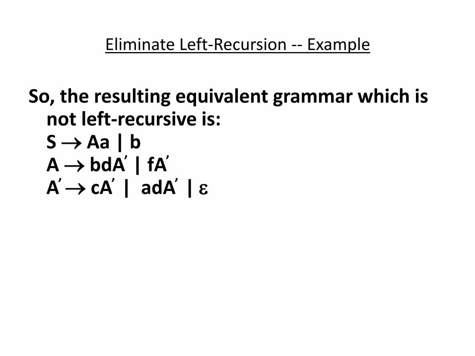
Eliminate Left-Recursion -- Example

So, the resulting equivalent grammar which is not left-recursive is:

S Aa | b A bdA | fA

A cA | adA |

Eliminate Left-Recursion – Example2

S Aa | b A Ac | Sd | f - Order of non-terminals: A, S for A: - we do not enter the inner loop. - Eliminate the immediate left-recursion in A A SdA | fA

A cA |

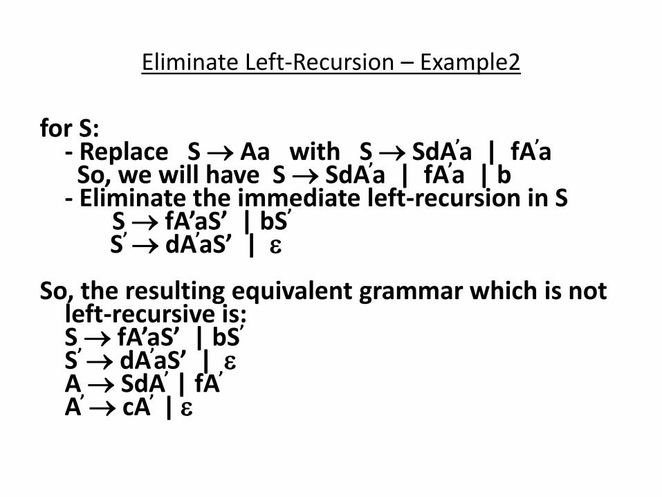
Eliminate Left-Recursion – Example2

for S: - Replace S Aa with S SdAa | fAa So, we will have S SdAa | fAa | b - Eliminate the immediate left-recursion in S S fA a“ | “

S dAa“ | So, the resulting equivalent grammar which is not

left-recursive is: S fA a“ | “

S dAa“ | A SdA | fA

A cA |

Left-Factoring

• A predictive parser (a top-down parser without backtracking) insists that the grammar must be left-factored.

grammar a new equivalent grammar suitable for predictive parsing

stmt if expr then stmt else stmt |

if expr then stmt

• when we see if, we cannot now which production rule to choose to re-write stmt in the derivation.

Left-Factoring (cont.)

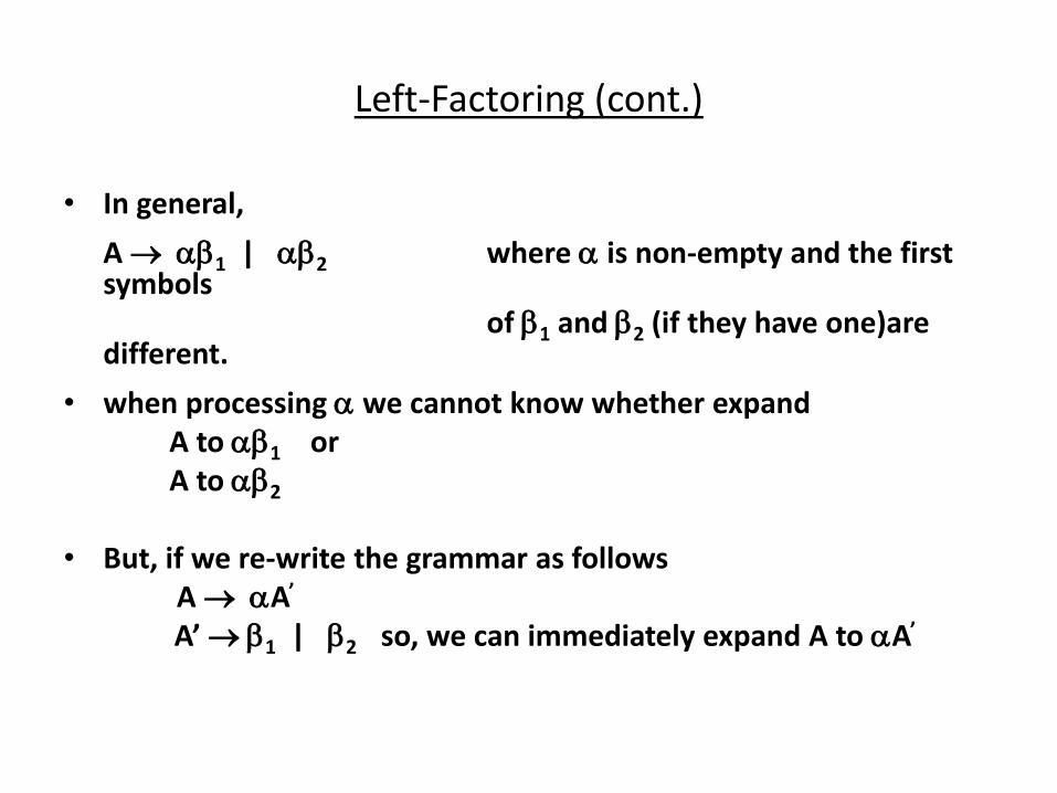
• In general,

A 1 | 2 where is non-empty and the first symbols

of 1 and 2 (if they have one)are different.

• when processing we cannot know whether expand

A to 1 or

A to 2

• But, if we re-write the grammar as follows

A A

A 1 | 2 so, we can immediately expand A to A

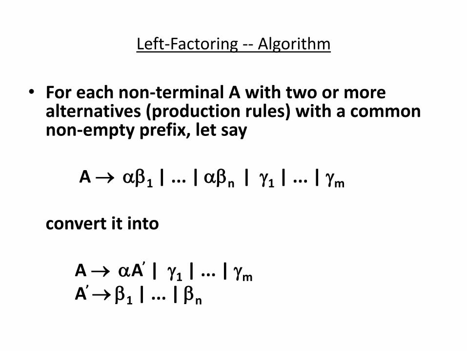
Left-Factoring -- Algorithm

• For each non-terminal A with two or more alternatives (production rules) with a common non-empty prefix, let say

A 1 | ... | n | 1 | ... | m

convert it into

A A | 1 | ... | m

A 1 | ... | n

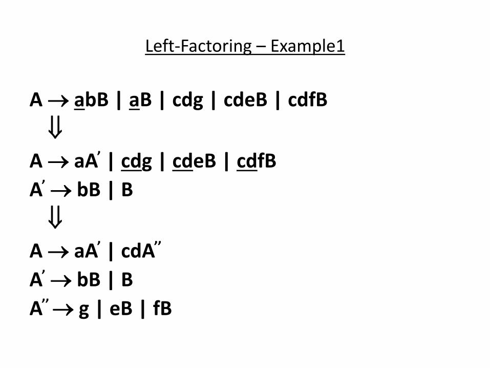
Left-Factoring – Example1

A abB | aB | cdg | cdeB | cdfB

A aA | cdg | cdeB | cdfB

A bB | B

A aA | cdA

A bB | B

A g | eB | fB

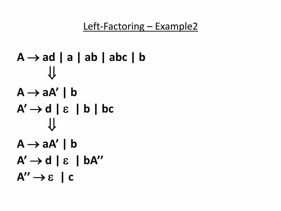
Left-Factoring – Example2

A ad | a | ab | abc | b

A aA |

A d | | b | bc

A aA |

A d | | A

A | c

Non-Recursive Predictive Parsing -- LL(1) Parser

• Non-Recursive predictive parsing is a table-driven parser.

• It is a top-down parser.

• It is also known as LL(1) Parser.

input buffer

stack Non-recursive output

Predictive Parser

Parsing Table

LL(1) Parser

input buffer – our string to be parsed. We will assume that its end is marked with a

special symbol $.

output

– a production rule representing a step of the derivation sequence (left-most derivation) of the string in the input buffer.

stack

– contains the grammar symbols – at the bottom of the stack, there is a special end marker symbol $. – initially the stack contains only the symbol $ and the starting symbol

S. $S initial stack

LL(1) Parser

– when the stack is emptied (ie. only $ left in the stack), the parsing is completed.

parsing table – a two-dimensional array M[A,a]

– each row is a non-terminal symbol

– each column is a terminal symbol or the special symbol $

– each entry holds a production rule.

LL(1) Parser – Parser Actions

• The symbol at the top of the stack (say X) and the current symbol in the input string (say a) determine the parser action.

• There are four possible parser actions.

1. If X and a are $ parser halts (successful completion)

2. If X and a are the same terminal symbol (different from $)

parser pops X from the stack, and moves the next symbol in the input buffer.

LL(1) Parser – Parser Actions

3. If X is a non-terminal parser looks at the parsing table entry

M[X,a]. If M[X,a] holds a production rule XY1Y2...Yk, it pops X from the stack and pushes Yk,Yk-1,...,Y1 into the stack. The parser also outputs the production rule XY1Y2...Yk to represent a step of the derivation.

4. none of the above error

– all empty entries in the parsing table are errors. – If X is a terminal symbol different from a, this is also an error

case.

LL(1) Parser – Example1

S aBa LL(1) Parsing

B bB | Table stack input output $S abba$ S aBa $aBa abba$ $aB bba$ B bB $aBb bba$ $aB ba$ B bB $aBb ba$

a b $

S S aBa

B B B bB

LL(1) Parser – Example1

$aB a$ B

$a a$

$ $ accept, successful completion

LL(1) Parser – Example1 (cont.)

Outputs: S aBa B bB B bB B

Derivation(left-most): SaBaabBaabbBaabba

S

B a a

B

B b

b

parse tree

LL(1) Parser – Example2

E TE

E +TE |

T FT

T *FT |

F (E) | id

id + * ( ) $

E E TE’

E TE’

E’ E’ +TE’ E’ E’ T T

FT’ T FT’

T’ T’ T’

*FT’ T’ T’

F F id F (E)

LL(1) Parser – Example2

stack input output

$E id+id$ E TE’

$E’T id+id$ T FT’

$E’ T’F id+id$ F id

$ E’ T’id id+id$

$ E’ T’ +id$ T’

$ E’ +id$ E’ +TE’

$ E’ T+ +id$

$ E’ T id$ T FT’

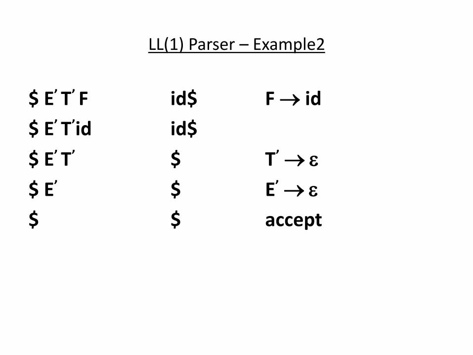
LL(1) Parser – Example2

$ E T F id$ F id

$ E T id id$

$ E T $ T

$ E $ E

$ $ accept

Constructing LL(1) Parsing Tables

• Two functions are used in the construction of LL(1) parsing tables: – FIRST FOLLOW

• FIRST() is a set of the terminal symbols which occur as first

symbols in strings derived from where is any string of grammar symbols.

• if derives to , then is also in FIRST() .

• FOLLOW(A) is the set of the terminals which occur immediately after (follow) the non-terminal A in the strings derived from the starting symbol. – a terminal a is in FOLLOW(A) if S Aa – $ is in FOLLOW(A) if S A

*

*

Compute FIRST for Any String X

• If X is a terminal symbol FIRST(X)={X} • If X is a non-terminal symbol and X is a production rule

is in FIRST(X). • If X is a non-terminal symbol and X Y1Y2..Yn is a production

rule if a terminal a in FIRST(Yi) and is in all FIRST(Yj) for j=1,...,i-1 then a is in FIRST(X). if is in all FIRST(Yj) for j=1,...,n then is in FIRST(X).

• If X is FIRST(X)={} • If X is Y1Y2..Yn

if a terminal a in FIRST(Yi) and is in all FIRST(Yj) for j=1,...,i-1 then a is in FIRST(X). if is in all FIRST(Yj) for j=1,...,n then is in FIRST(X).

FIRST Example

E TE

E +TE |

T FT

T *FT |

F (E) | id FIRST(F) = {(,id} FIRST(TE’) = {(,id} FIRST(T’) = {*, } FIRST(+TE’ ) = {+} FIRST(T) = {(,id} FIRST() = {} FIRST(E’) = {+, } FIRST(FT’) = {(,id} FIRST(E) = {(,id} FIRST(*FT’) = {*} FIRST() = {} FIRST((E)) = {(} FIRST(id) = {id}

Compute FOLLOW (for non-terminals)

• If S is the start symbol $ is in FOLLOW(S)

• if A B is a production rule everything in FIRST() is FOLLOW(B) except

• If ( A B is a production rule ) or ( A B is a production rule and is in FIRST() ) everything in FOLLOW(A) is in FOLLOW(B).

We apply these rules until nothing more can be added to any follow set.

FOLLOW Example

E TE

E +TE |

T FT

T *FT |

F (E) | id

FOLLOW(E) = { $, ) }

FOLLOW(E ) = { $, ) }

FOLLOW(T) = { +, ), $ }

FOLLOW(T ) = { +, ), $ }

FOLLOW(F) = {+, *, ), $ }

Constructing LL(1) Parsing Table -- Algorithm

• for each production rule A of a grammar G – for each terminal a in FIRST()

add A to M[A,a]

– If in FIRST()

for each terminal a in FOLLOW(A) add A to M[A,a]

– If in FIRST() and $ in FOLLOW(A)

add A to M[A,$]

• All other undefined entries of the parsing table

are error entries.

Constructing LL(1) Parsing Table -- Example

E TE FIRST(TE )={(,id} E TE into M[E,(] and M[E,id]

E +TE FIRST(+TE )={+} E +TE into M[E,+]

E FIRST()={} none but since in FIRST() and FOLLOW(E )={$,)} E into

M[E,$] and M[E,)] T FT FIRST(FT )={(,id} T FT into

M[T,(] and M[T,id]

T *FT FIRST(*FT )={*} T *FT into M[T ,*]

Constructing LL(1) Parsing Table -- Example

T FIRST()={} none but since in FIRST() and FOLLOW(T )={$,),+} T

into M[T ,$], M[T ,)] and M[T ,+] F (E) FIRST((E) )={(} F

(E) into M[F,(] F id FIRST(id)={id} F id

into M[F,id]

LL(1) Grammars

• A grammar whose parsing table has no multiply-defined entries is said to be LL(1) grammar.

one input symbol used as a look-head symbol do determine parser action

LL(1) left most derivation

input scanned from left to right

• The parsing table of a grammar may contain more than one production rule. In this case, we say that it is not a LL(1) grammar.

A Grammar which is not LL(1)

S i C t S E | a FOLLOW(S) = { $,e } E e S | FOLLOW(E) = { $,e } C b FOLLOW(C) = { t } FIRST(iCtSE) = {i} FIRST(a) = {a} FIRST(eS) = {e} FIRST() = {} FIRST(b) = {b} two production rules for M[E,e] Problem ambiguity

a b e i t $

S S a S

iCtSE

E E e S

E E

C C b

A Grammar which is not LL(1) (cont.)

• What do we have to do it if the resulting

parsing table contains multiply defined

entries? – If e did t eli i ate left e u sio , eli i ate the left

recursion in the grammar.

– If the grammar is not left factored, we have to left factor

the grammar.

– If its e g a a s pa si g ta le still o tai s ultipl defined entries, that grammar is ambiguous or it is

inherently not a LL(1) grammar.

A Grammar which is not LL(1) (cont.)

• A left recursive grammar cannot be a LL(1) grammar. – A A |

any terminal that appears in FIRST() also appears FIRST(A) because A .

If is , any terminal that appears in FIRST() also appears in FIRST(A) and FOLLOW(A).

• A grammar is not left factored, it cannot be a LL(1) grammar • A 1 | 2

any terminal that appears in FIRST(1) also appears in FIRST(2).

• An ambiguous grammar cannot be a LL(1) grammar.

Properties of LL(1) Grammars

• A grammar G is LL(1) if and only if the following conditions hold for two distinctive production rules A and A

1. Both and cannot derive strings starting with same

terminals.

2. At most one of and can derive to .

3. If can derive to , then cannot derive to any string starting with a terminal in FOLLOW(A).

Error Recovery in Predictive Parsing

• An error may occur in the predictive parsing

(LL(1) parsing) – if the terminal symbol on the top of stack does not match with

the current input symbol.

– if the top of stack is a non-terminal A, the current input symbol

is a, and the parsing table entry M[A,a] is empty.

• What should the parser do in an error case? – The parser should be able to give an error message (as much

as possible meaningful error message).

– It should be recover from that error case, and it should be able

to continue the parsing with the rest of the input.

Error Recovery Techniques

• Panic-Mode Error Recovery – Skipping the input symbols until a synchronizing token is

found.

• Phrase-Level Error Recovery – Each empty entry in the parsing table is filled with a pointer to

a specific error routine to take care that error case.

• Error-Productions – If we have a good idea of the common errors that might be

encountered, we can augment the grammar with productions that generate erroneous constructs.

– When an error production is used by the parser, we can generate appropriate error diagnostics.

– Since it is almost impossible to know all the errors that can be made by the programmers, this method is not practical.

Error Recovery Techniques

• Global-Correction – Ideally, we would like a compiler to make as few change

as possible in processing incorrect inputs.

– We have to globally analyze the input to find the error.

– This is an expensive method, and it is not in practice.

Panic-Mode Error Recovery in LL(1) Parsing

• In panic-mode error recovery, we skip all the input symbols until a synchronizing token is found.

• What is the synchronizing token? – All the terminal-symbols in the follow set of a non-terminal can be

used as a synchronizing token set for that non-terminal.

• So, a simple panic-mode error recovery for the LL(1) parsing: – All the empty entries are marked as synch to indicate that the

parser will skip all the input symbols until a symbol in the follow set of the non-terminal A which on the top of the stack. Then the parser will pop that non-terminal A from the stack. The parsing continues from that state.

– To handle unmatched terminal symbols, the parser pops that unmatched terminal symbol from the stack and it issues an error message saying that that unmatched terminal is inserted.

Panic-Mode Error Recovery - Example

S AbS | e | A a | cAd

FOLLOW(S)={$} FOLLOW(A)={b,d}

stack input output stack input

output $S aab$ S AbS $S ceadb$

S AbS $SbA aab$ A a $SbA ceadb$

A cAd $Sba aab$ $SbdAc ceadb$

$Sb ab$ $SbdA eadb$

a b c d e $

S S

AbS

syn

c

S AbS syn

c

S

e

S

A A a syn

c

A cAd syn

c

sync sync

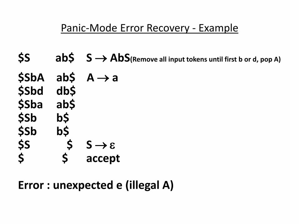
Panic-Mode Error Recovery - Example

$S ab$ S AbS(Remove all input tokens until first b or d, pop A)

$SbA ab$ A a $Sbd db$ $Sba ab$ $Sb b$ $Sb b$ $S $ S $ $ accept Error : unexpected e (illegal A)

Phrase-Level Error Recovery

• Each empty entry in the parsing table is filled with a pointer to a special error routine which will take care that error case.

• These error routines may: – change, insert, or delete input symbols.

– issue appropriate error messages

– pop items from the stack.

• We should be careful when we design these error routines, because we may put the parser into an infinite loop.

Unit-2

Bottom - Up Parsing

Bottom-Up Parsing

• A bottom-up parser creates the parse tree of the given input starting from leaves towards the root.

• A bottom-up parser tries to find the right-most derivation of the given input in the reverse order. S ... (the right-most derivation of )

(the bottom-up parser finds the right-most derivation in the reverse order)

• Bottom-up parsing is also known as shift-reduce parsing because its two main actions are shift and reduce. – At each shift action, the current symbol in the input string is pushed

to a stack.

Bottom-Up Parsing

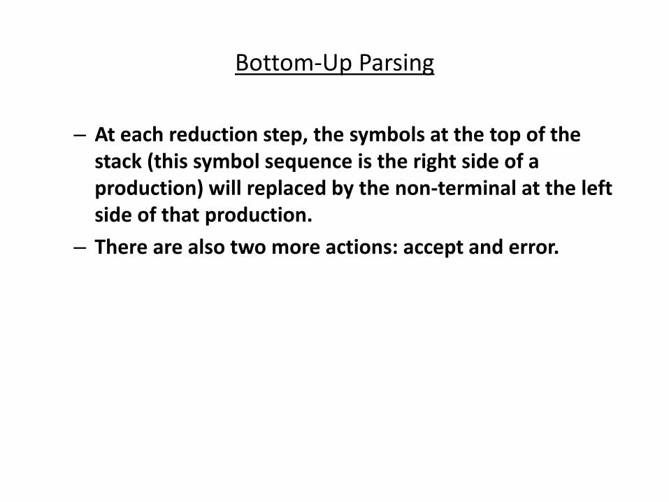
– At each reduction step, the symbols at the top of the

stack (this symbol sequence is the right side of a

production) will replaced by the non-terminal at the left

side of that production.

– There are also two more actions: accept and error.

Shift-Reduce Parsing

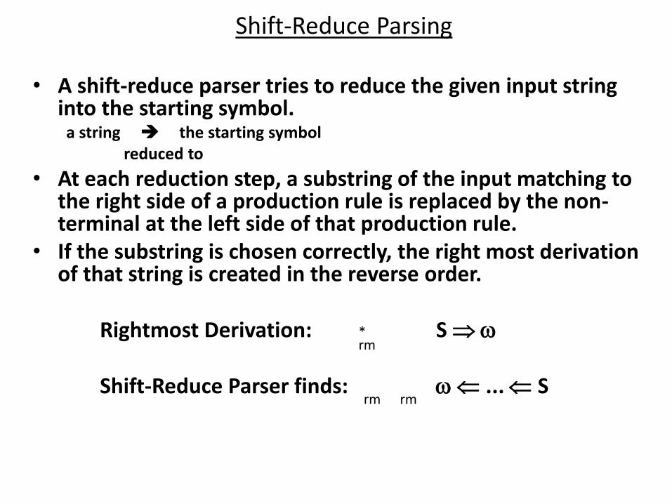
• A shift-reduce parser tries to reduce the given input string into the starting symbol.

a string the starting symbol

reduced to

• At each reduction step, a substring of the input matching to the right side of a production rule is replaced by the non-terminal at the left side of that production rule.

• If the substring is chosen correctly, the right most derivation of that string is created in the reverse order.

Rightmost Derivation: S

Shift-Reduce Parser finds: ... S

* rm

rm rm

Shift-Reduce Parsing -- Example

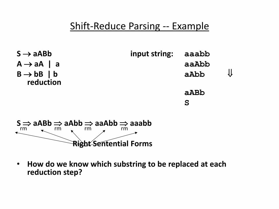
S aABb input string: aaabb

A aA | a aaAbb

B bB | b aAbb reduction

aABb S S aABb aAbb aaAbb aaabb

Right Sentential Forms

• How do we know which substring to be replaced at each reduction step?

rm rm rm rm

Handle

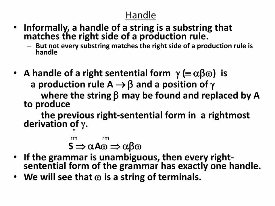
• Informally, a handle of a string is a substring that matches the right side of a production rule. – But not every substring matches the right side of a production rule is

handle

• A handle of a right sentential form ( ) is a production rule A and a position of where the string may be found and replaced by A

to produce the previous right-sentential form in a rightmost

derivation of . S A • If the grammar is unambiguous, then every right-

sentential form of the grammar has exactly one handle. • We will see that is a string of terminals.

rm rm *

Handle Pruning

• A right-most derivation in reverse can be obtained by handle-pruning.

S=0 1 2 ... n-1 n=

input string

• Start from n, find a handle Ann in n, and replace n in by An to get n-1.

• Then find a handle An-1n-1 in n-1, and replace n-1 in by An-1 to get n-2.

• Repeat this, until we reach S.

rm rm rm rm rm

A Shift-Reduce Parser

E E+T | T Right-Most Derivation of id+id*id T T*F | F E E+T E+T*F E+T*id E+F*id F (E) | id E+id*id T+id*id F+id*id id+id*id Right-Most Sentential Form Reducing Production id+id*id F id F+id*id T F T+id*id E T E+id*id F id E+F*id T F E+T*id F id E+T*F T T*F E+T E E+T E Handles are red and underlined in the right-sentential

forms.

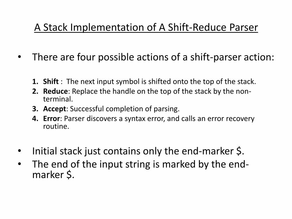
A Stack Implementation of A Shift-Reduce Parser

• There are four possible actions of a shift-parser action:

1. Shift : The next input symbol is shifted onto the top of the stack.

2. Reduce: Replace the handle on the top of the stack by the non-terminal.

3. Accept: Successful completion of parsing.

4. Error: Parser discovers a syntax error, and calls an error recovery routine.

• Initial stack just contains only the end-marker $.

• The end of the input string is marked by the end-marker $.

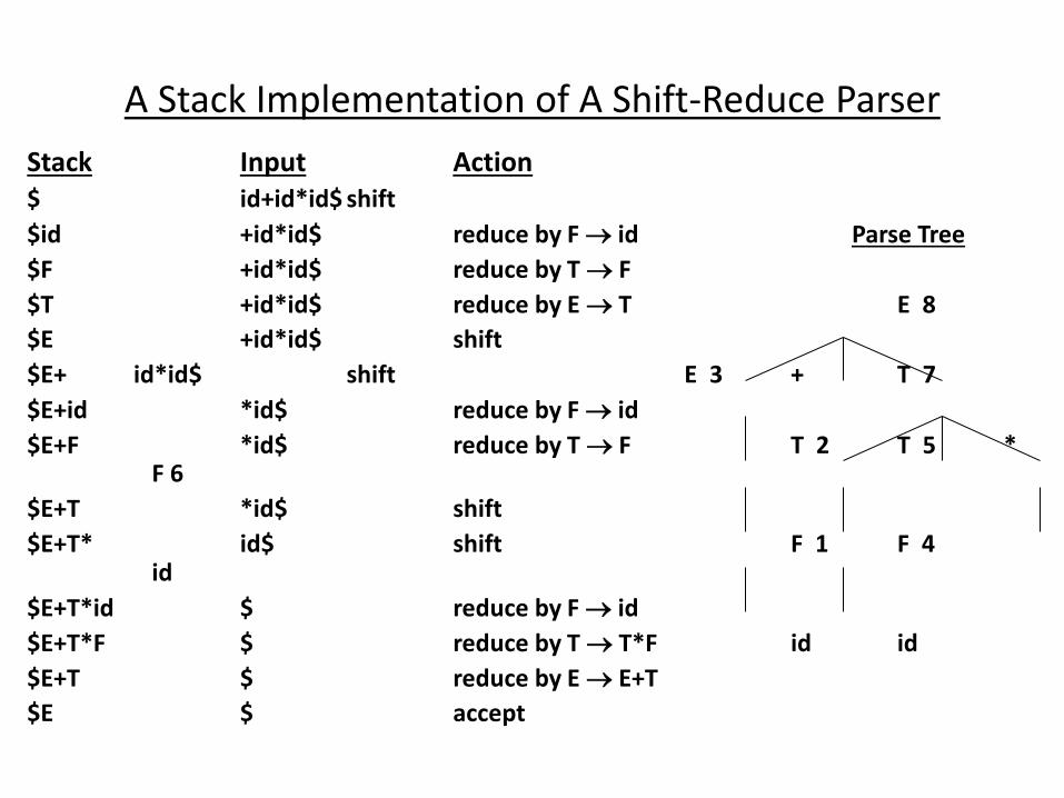
A Stack Implementation of A Shift-Reduce Parser

Stack Input Action

$ id+id*id$ shift

$id +id*id$ reduce by F id Parse Tree

$F +id*id$ reduce by T F

$T +id*id$ reduce by E T E 8

$E +id*id$ shift

$E+ id*id$ shift E 3 + T 7

$E+id *id$ reduce by F id

$E+F *id$ reduce by T F T 2 T 5 * F 6

$E+T *id$ shift

$E+T* id$ shift F 1 F 4 id

$E+T*id $ reduce by F id

$E+T*F $ reduce by T T*F id id

$E+T $ reduce by E E+T

$E $ accept

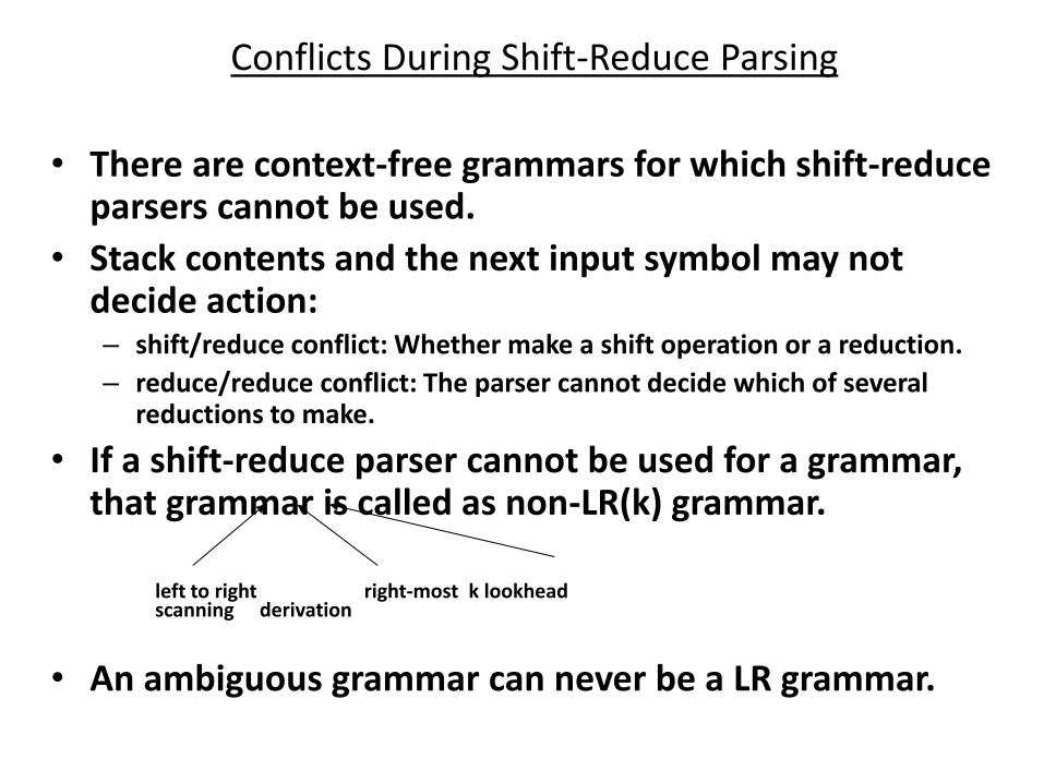
Conflicts During Shift-Reduce Parsing

• There are context-free grammars for which shift-reduce parsers cannot be used.

• Stack contents and the next input symbol may not decide action: – shift/reduce conflict: Whether make a shift operation or a reduction.

– reduce/reduce conflict: The parser cannot decide which of several reductions to make.

• If a shift-reduce parser cannot be used for a grammar, that grammar is called as non-LR(k) grammar.

left to right right-most k lookhead scanning derivation

• An ambiguous grammar can never be a LR grammar.

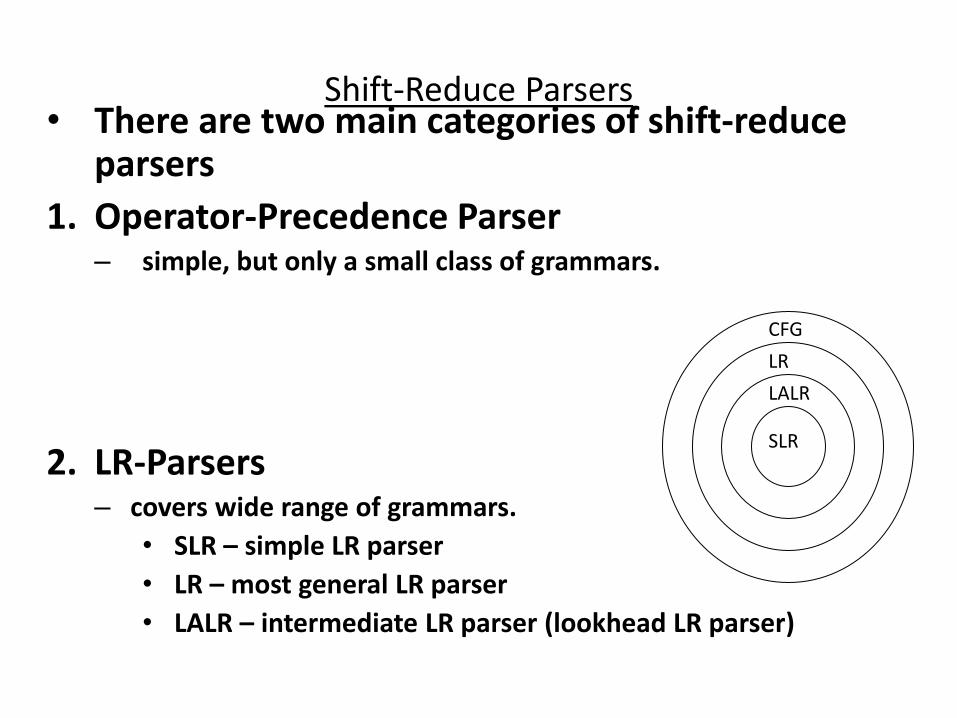
Shift-Reduce Parsers • There are two main categories of shift-reduce

parsers

1. Operator-Precedence Parser – simple, but only a small class of grammars.

2. LR-Parsers – covers wide range of grammars.

• SLR – simple LR parser

• LR – most general LR parser

• LALR – intermediate LR parser (lookhead LR parser)

SLR

CFG

LR

LALR

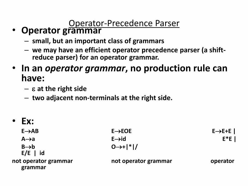
Operator-Precedence Parser • Operator grammar

– small, but an important class of grammars

– we may have an efficient operator precedence parser (a shift-reduce parser) for an operator grammar.

• In an operator grammar, no production rule can have: – at the right side

– two adjacent non-terminals at the right side.

• Ex: EAB EEOE EE+E |

Aa Eid E*E |

Bb O+|*|/ E/E | id

not operator grammar not operator grammar operator grammar

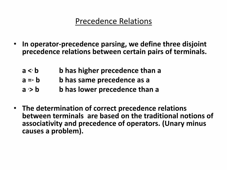
Precedence Relations

• In operator-precedence parsing, we define three disjoint precedence relations between certain pairs of terminals.

a <. b b has higher precedence than a

a =· b b has same precedence as a

a .> b b has lower precedence than a

• The determination of correct precedence relations between terminals are based on the traditional notions of associativity and precedence of operators. (Unary minus causes a problem).

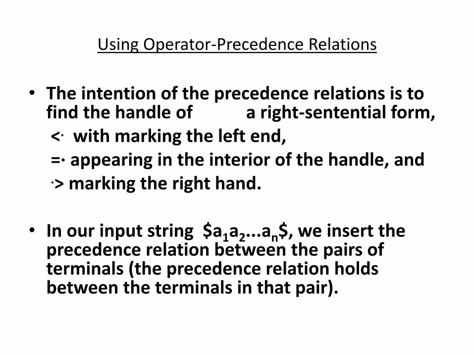
Using Operator-Precedence Relations

• The intention of the precedence relations is to find the handle of a right-sentential form,

<. with marking the left end,

=· appearing in the interior of the handle, and

.> marking the right hand.

• In our input string $a1a2...an$, we insert the precedence relation between the pairs of terminals (the precedence relation holds between the terminals in that pair).

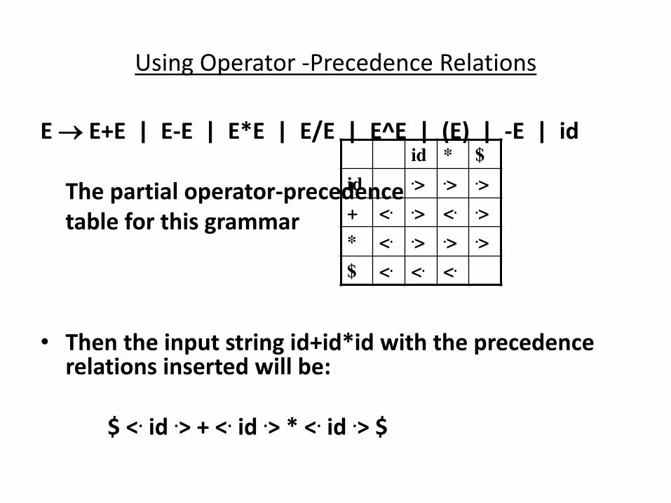
Using Operator -Precedence Relations

E E+E | E-E | E*E | E/E | E^E | (E) | -E | id

The partial operator-precedence

table for this grammar

• Then the input string id+id*id with the precedence relations inserted will be:

$ <. id .> + <. id .> * <. id .> $

id * $

id .> .> .>

+ <. .> <. .>

* <. .> .> .>

$ <. <. <.

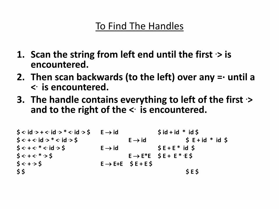
To Find The Handles

1. Scan the string from left end until the first .> is encountered.

2. Then scan backwards (to the left) over any =· until a <. is encountered.

3. The handle contains everything to left of the first .> and to the right of the <. is encountered.

$ <. id .> + <. id .> * <. id .> $ E id $ id + id * id $

$ <. + <. id .> * <. id .> $ E id $ E + id * id $

$ <. + <. * <. id .> $ E id $ E + E * id $

$ <. + <. * .> $ E E*E $ E + E * .E $

$ <. + .> $ E E+E $ E + E $

$ $ $ E $

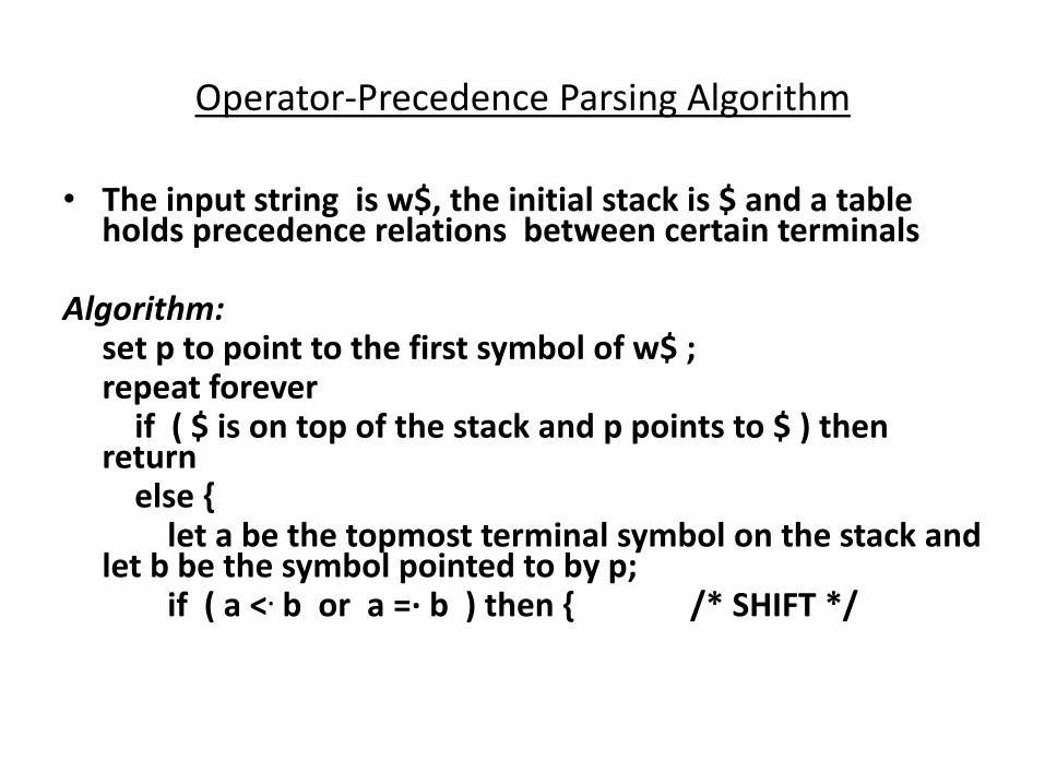
Operator-Precedence Parsing Algorithm

• The input string is w$, the initial stack is $ and a table holds precedence relations between certain terminals

Algorithm: set p to point to the first symbol of w$ ; repeat forever if ( $ is on top of the stack and p points to $ ) then

return else { let a be the topmost terminal symbol on the stack and

let b be the symbol pointed to by p; if ( a <. b or a =· b ) then { /* SHIFT */

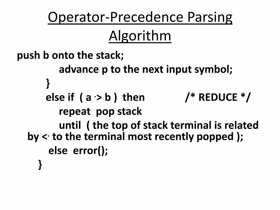
Operator-Precedence Parsing

Algorithm

push b onto the stack;

advance p to the next input symbol;

}

else if ( a .> b ) then /* REDUCE */

repeat pop stack

until ( the top of stack terminal is related by <. to the terminal most recently popped );

else error();

}

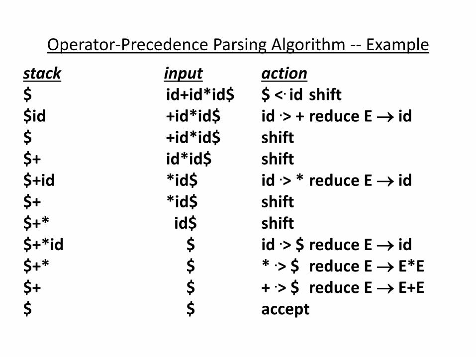
Operator-Precedence Parsing Algorithm -- Example

stack input action

$ id+id*id$ $ <. id shift

$id +id*id$ id .> + reduce E id

$ +id*id$ shift

$+ id*id$ shift

$+id *id$ id .> * reduce E id

$+ *id$ shift

$+* id$ shift

$+*id $ id .> $ reduce E id

$+* $ * .> $ reduce E E*E

$+ $ + .> $ reduce E E+E

$ $ accept

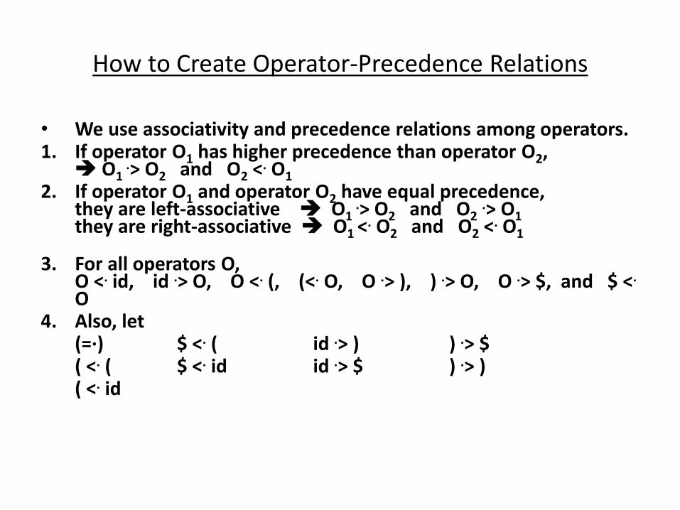
How to Create Operator-Precedence Relations

• We use associativity and precedence relations among operators. 1. If operator O1 has higher precedence than operator O2,

O1 .> O2 and O2 <. O1

2. If operator O1 and operator O2 have equal precedence, they are left-associative O1

.> O2 and O2 .> O1 they are right-associative O1 <

. O2 and O2 <. O1

3. For all operators O, O <. id, id .> O, O <. (, (<. O, O .> ), ) .> O, O .> $, and $ <. O

4. Also, let (=·) $ <. ( id .> ) ) .> $ ( <. ( $ <. id id .> $ ) .> ) ( <. id

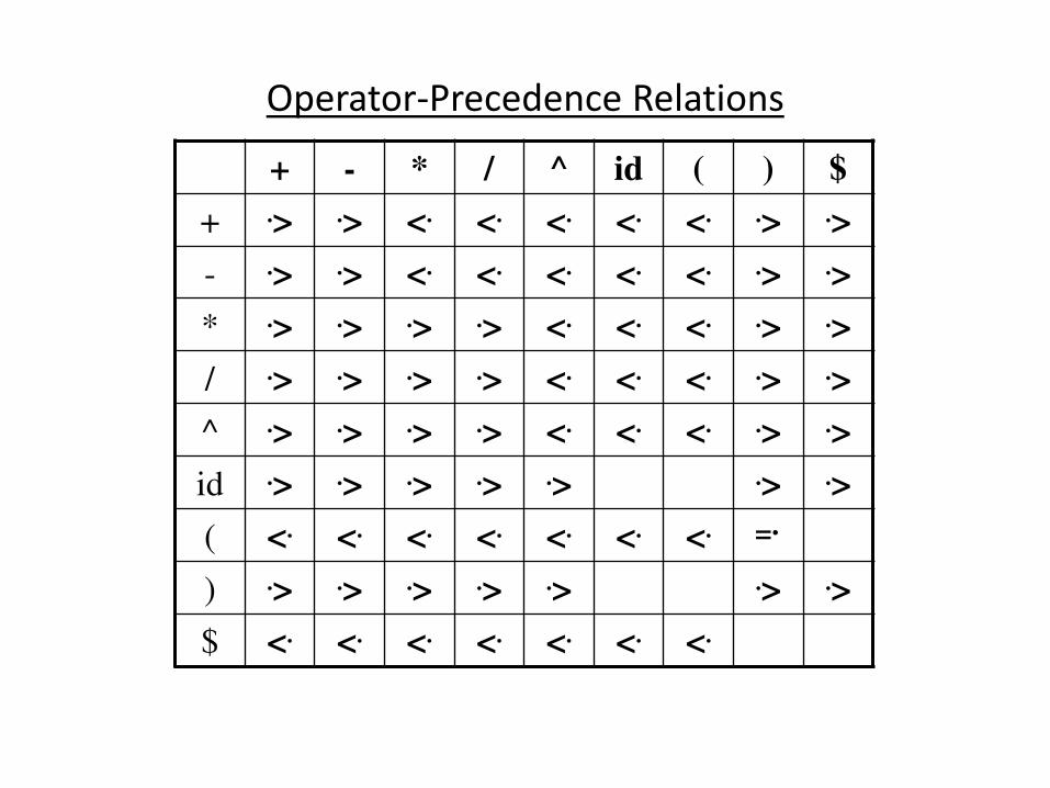
Operator-Precedence Relations

+ - * / ^ id ( ) $

+ .> .> <. <. <. <. <. .> .>

- .> .> <. <. <. <. <. .> .>

* .> .> .> .> <. <. <. .> .>

/ .> .> .> .> <. <. <. .> .>

^ .> .> .> .> <. <. <. .> .>

id .> .> .> .> .> .> .>

( <. <. <. <. <. <. <. =·

) .> .> .> .> .> .> .>

$ <. <. <. <. <. <. <.

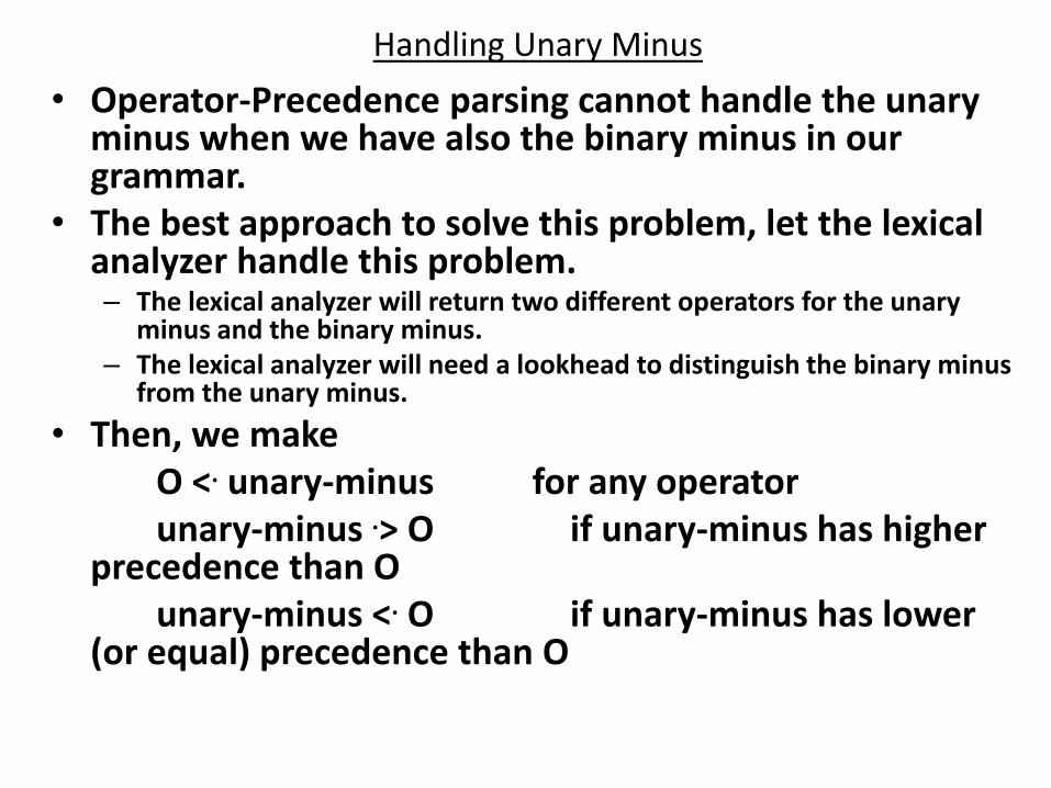
Handling Unary Minus

• Operator-Precedence parsing cannot handle the unary minus when we have also the binary minus in our grammar.

• The best approach to solve this problem, let the lexical analyzer handle this problem. – The lexical analyzer will return two different operators for the unary

minus and the binary minus.

– The lexical analyzer will need a lookhead to distinguish the binary minus from the unary minus.

• Then, we make

O <. unary-minus for any operator

unary-minus .> O if unary-minus has higher precedence than O

unary-minus <. O if unary-minus has lower (or equal) precedence than O

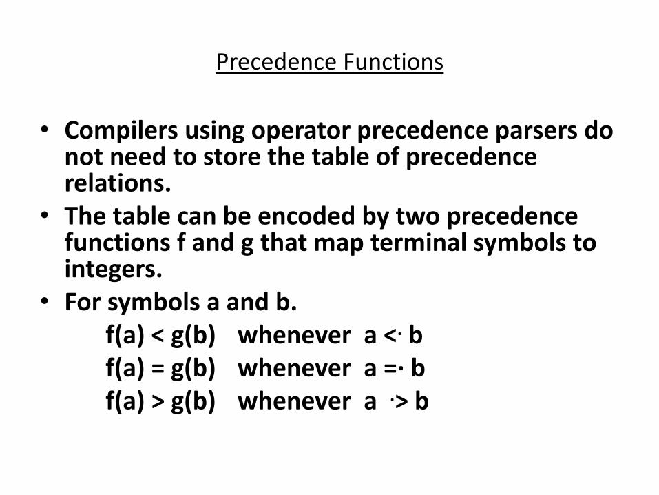
Precedence Functions

• Compilers using operator precedence parsers do not need to store the table of precedence relations.

• The table can be encoded by two precedence functions f and g that map terminal symbols to integers.

• For symbols a and b.

f(a) < g(b) whenever a <. b

f(a) = g(b) whenever a =· b

f(a) > g(b) whenever a .> b

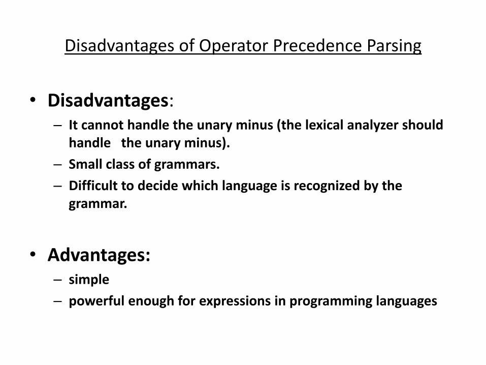
Disadvantages of Operator Precedence Parsing

• Disadvantages: – It cannot handle the unary minus (the lexical analyzer should

handle the unary minus).

– Small class of grammars.

– Difficult to decide which language is recognized by the

grammar.

• Advantages: – simple

– powerful enough for expressions in programming languages

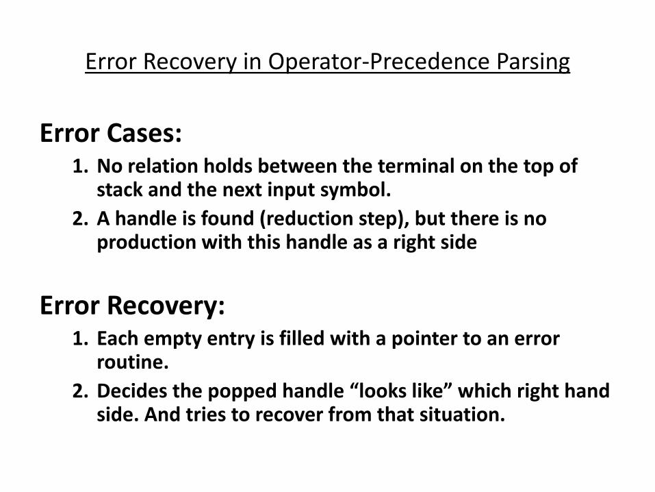
Error Recovery in Operator-Precedence Parsing

Error Cases: 1. No relation holds between the terminal on the top of

stack and the next input symbol.

2. A handle is found (reduction step), but there is no production with this handle as a right side

Error Recovery: 1. Each empty entry is filled with a pointer to an error

routine.

2. De ides the popped ha dle looks like hi h ight ha d side. And tries to recover from that situation.

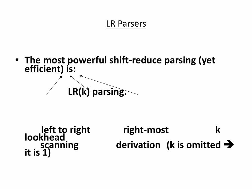
LR Parsers

• The most powerful shift-reduce parsing (yet

efficient) is:

LR(k) parsing.

left to right right-most k

lookhead scanning derivation (k is omitted

it is 1)

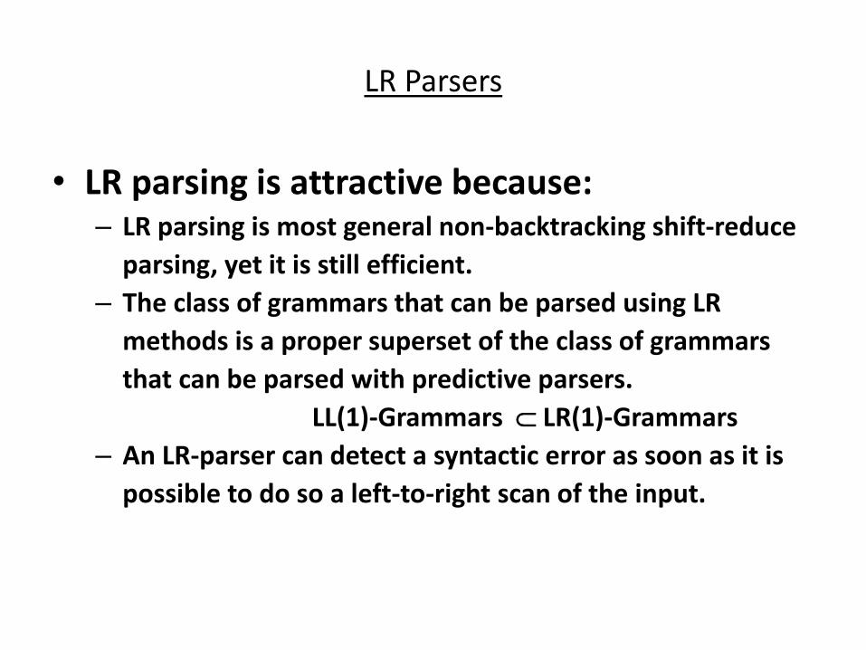
LR Parsers

• LR parsing is attractive because: – LR parsing is most general non-backtracking shift-reduce

parsing, yet it is still efficient.

– The class of grammars that can be parsed using LR

methods is a proper superset of the class of grammars

that can be parsed with predictive parsers.

LL(1)-Grammars LR(1)-Grammars

– An LR-parser can detect a syntactic error as soon as it is

possible to do so a left-to-right scan of the input.

LR Parsers

• LR-Parsers – covers wide range of grammars.

– SLR – simple LR parser

– CLR – most general LR parser

– LALR – intermediate LR parser (look-head LR parser)

– SLR, LR and LALR work same (they used the same

algorithm), only their parsing tables are different.

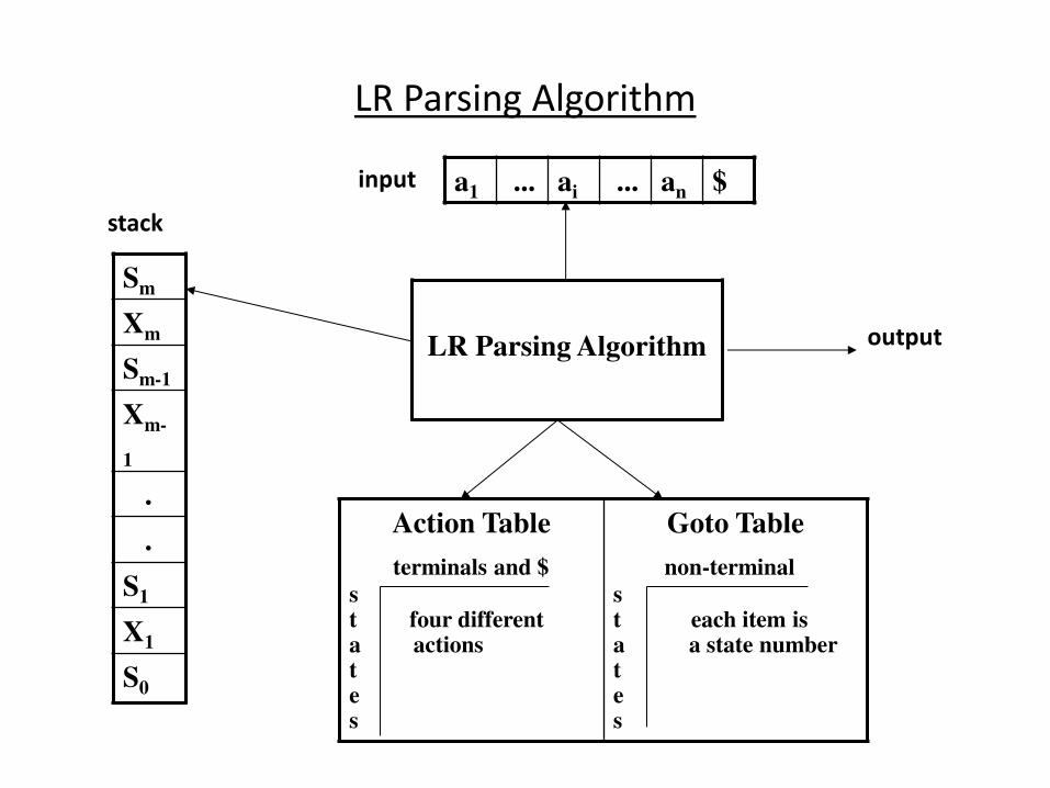
LR Parsing Algorithm

Sm

Xm

Sm-1

Xm-

1

.

.

S1

X1

S0

a1 ... ai ... an $

Action Table

terminals and $ s t four different a actions t e s

Goto Table

non-terminal s t each item is a a state number t e s

LR Parsing Algorithm

stack

input

output

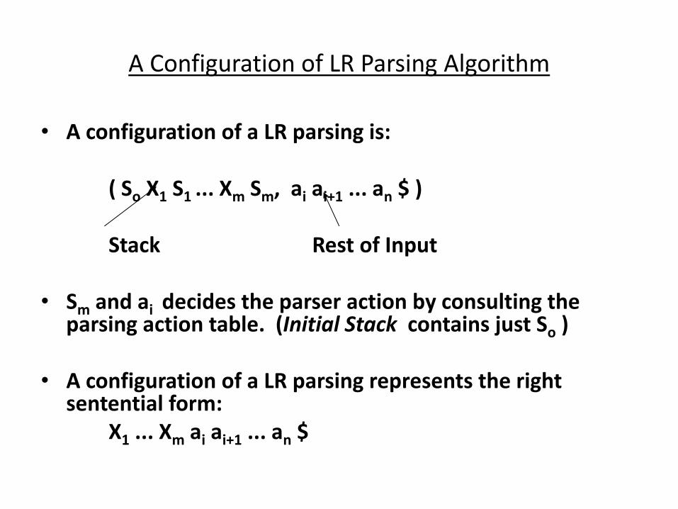
A Configuration of LR Parsing Algorithm

• A configuration of a LR parsing is:

( So X1 S1 ... Xm Sm, ai ai+1 ... an $ )

Stack Rest of Input

• Sm and ai decides the parser action by consulting the parsing action table. (Initial Stack contains just So )

• A configuration of a LR parsing represents the right sentential form:

X1 ... Xm ai ai+1 ... an $

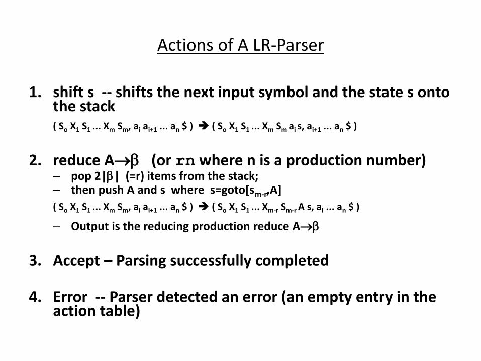
Actions of A LR-Parser

1. shift s -- shifts the next input symbol and the state s onto the stack

( So X1 S1 ... Xm Sm, ai ai+1 ... an $ ) ( So X1 S1 ... Xm Sm ai s, ai+1 ... an $ )

2. reduce A (or rn where n is a production number)

– pop 2|| (=r) items from the stack; – then push A and s where s=goto[sm-r,A]

( So X1 S1 ... Xm Sm, ai ai+1 ... an $ ) ( So X1 S1 ... Xm-r Sm-r A s, ai ... an $ )

– Output is the reducing production reduce A

3. Accept – Parsing successfully completed

4. Error -- Parser detected an error (an empty entry in the

action table)

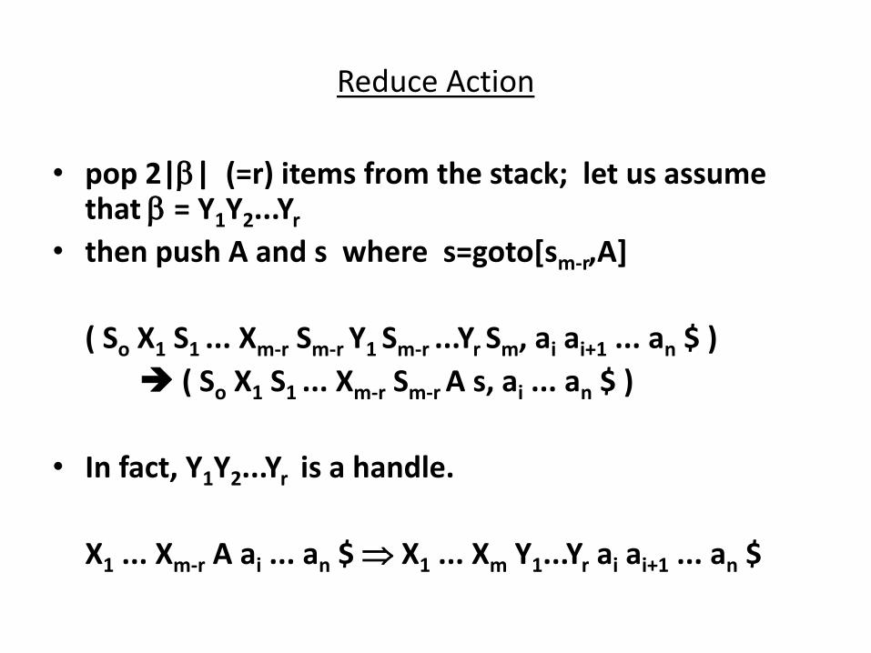
Reduce Action

• pop 2|| (=r) items from the stack; let us assume that = Y1Y2...Yr

• then push A and s where s=goto[sm-r,A]

( So X1 S1 ... Xm-r Sm-r Y1 Sm-r ...Yr Sm, ai ai+1 ... an $ )

( So X1 S1 ... Xm-r Sm-r A s, ai ... an $ )

• In fact, Y1Y2...Yr is a handle.

X1 ... Xm-r A ai ... an $ X1 ... Xm Y1...Yr ai ai+1 ... an $

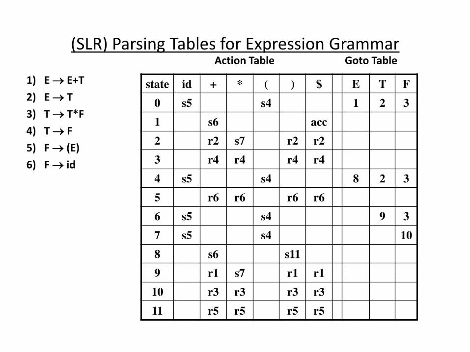
(SLR) Parsing Tables for Expression Grammar

state id + * ( ) $ E T F

0 s5 s4 1 2 3

1 s6 acc

2 r2 s7 r2 r2

3 r4 r4 r4 r4

4 s5 s4 8 2 3

5 r6 r6 r6 r6

6 s5 s4 9 3

7 s5 s4 10

8 s6 s11

9 r1 s7 r1 r1

10 r3 r3 r3 r3

11 r5 r5 r5 r5

Action Table Goto Table

1) E E+T

2) E T

3) T T*F

4) T F

5) F (E)

6) F id

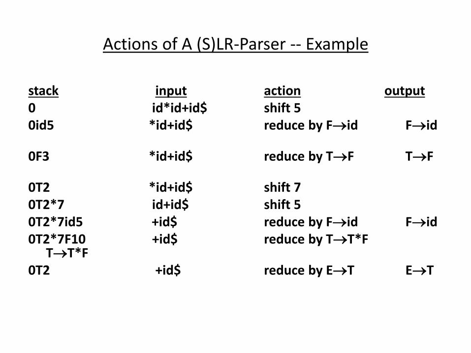
Actions of A (S)LR-Parser -- Example

stack input action output

0 id*id+id$ shift 5

0id5 *id+id$ reduce by Fid Fid

0F3 *id+id$ reduce by TF TF

0T2 *id+id$ shift 7

0T2*7 id+id$ shift 5

0T2*7id5 +id$ reduce by Fid Fid

0T2*7F10 +id$ reduce by TT*F TT*F

0T2 +id$ reduce by ET ET

Actions of A (S)LR-Parser -- Example

0E1 +id$ shift 6

0E1+6 id$ shift 5

0E1+6id5 $ reduce by Fid

0E1+6F3 $ reduce by TF

0E1+6T9 $ reduce by EE+T

0E1 $ accept

Constructing SLR Parsing Tables – LR(0) Item

• An LR(0) item of a grammar G is a production of G a dot at the some position of the right side.

• Ex: A aBb Possible LR(0) Items: A .aBb

(four different possibility) A a.Bb

A aB.b

A aBb.

• Sets of LR(0) items will be the states of action and goto table of the SLR parser.

• A collection of sets of LR(0) items (the canonical LR(0) collection) is the basis for constructing SLR parsers.

• Augmented Grammar:

G is G ith a e p odu tio ule “ “ he e “ is the e starting symbol.

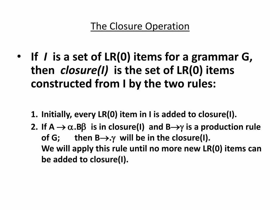
The Closure Operation

• If I is a set of LR(0) items for a grammar G, then closure(I) is the set of LR(0) items constructed from I by the two rules:

1. Initially, every LR(0) item in I is added to closure(I).

2. If A .B is in closure(I) and B is a production rule

of G; then B. will be in the closure(I).

We will apply this rule until no more new LR(0) items can

be added to closure(I).

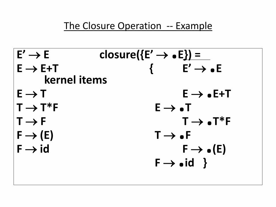
The Closure Operation -- Example

E E losu e {E .E}) = E E+T { E .E

kernel items E T E .E+T T T*F E .T T F T .T*F F (E) T .F F id F .(E) F .id }

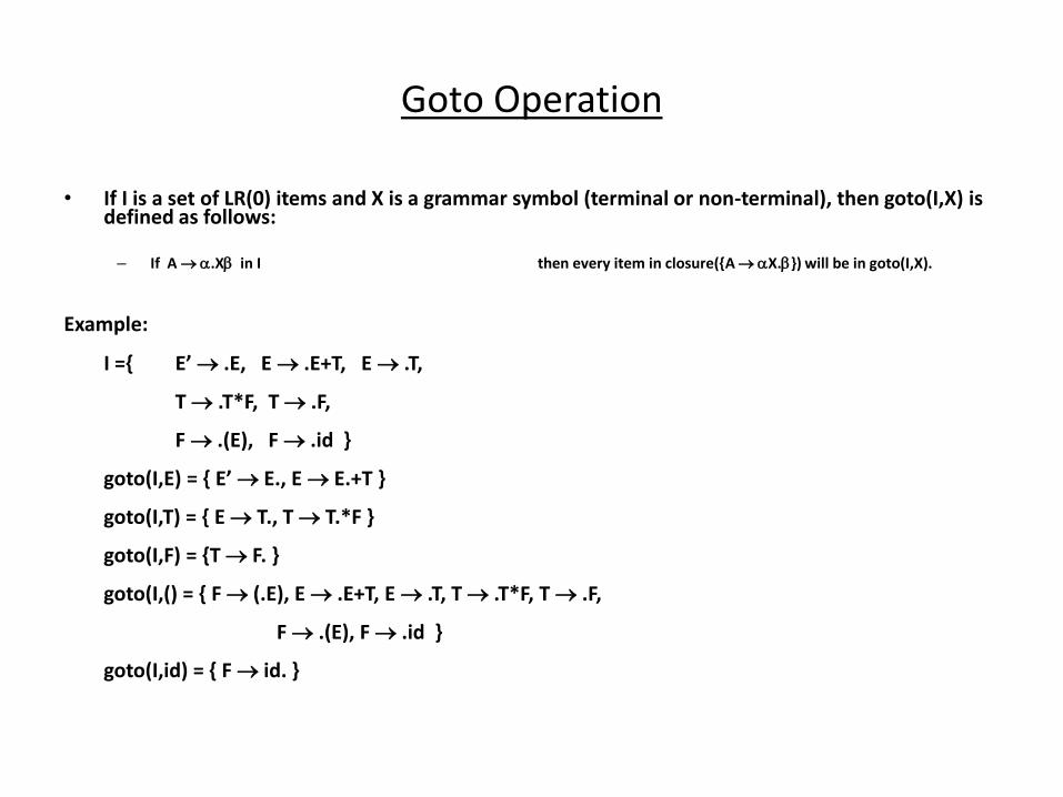
Goto Operation

• If I is a set of LR(0) items and X is a grammar symbol (terminal or non-terminal), then goto(I,X) is defined as follows:

– If A .X in I then every item in closure({A X.}) will be in goto(I,X).

Example:

I ={ E .E, E .E+T, E .T,

T .T*F, T .F,

F .(E), F .id }

goto I,E = { E E., E E.+T }

goto(I,T) = { E T., T T.*F }

goto(I,F) = {T F. }

goto(I,() = { F (.E), E .E+T, E .T, T .T*F, T .F,

F .(E), F .id }

goto(I,id) = { F id. }

Construction of The Canonical LR(0) Collection

• To create the SLR parsing tables for a grammar G, we will eate the a o i al L‘ olle tio of the g a a G .

• Algorithm:

C is { losu e {“ .S}) }

repeat the followings until no more set of LR(0) items can be added to C.

for each I in C and each grammar symbol X

if goto(I,X) is not empty and not in C

add goto(I,X) to C

• goto function is a DFA on the sets in C.

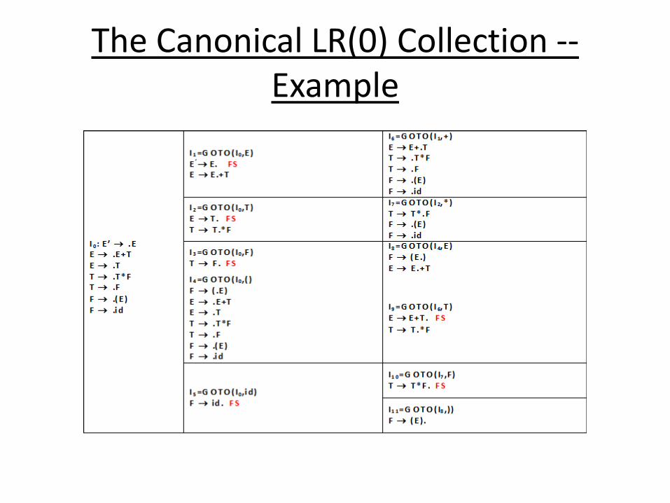
The Canonical LR(0) Collection --

Example

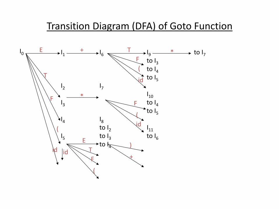
Transition Diagram (DFA) of Goto Function

I0 I1

I2

I3

I4

I5

I6

I7

I8

to I2

to I3

to I4

I9

to I3

to I4

to I5

I10

to I4

to I5

I11

to I6

to I7

id

(

F

*

E

E

+ T

T

T

)

F

F F

(

id id

(

*

(

id

+

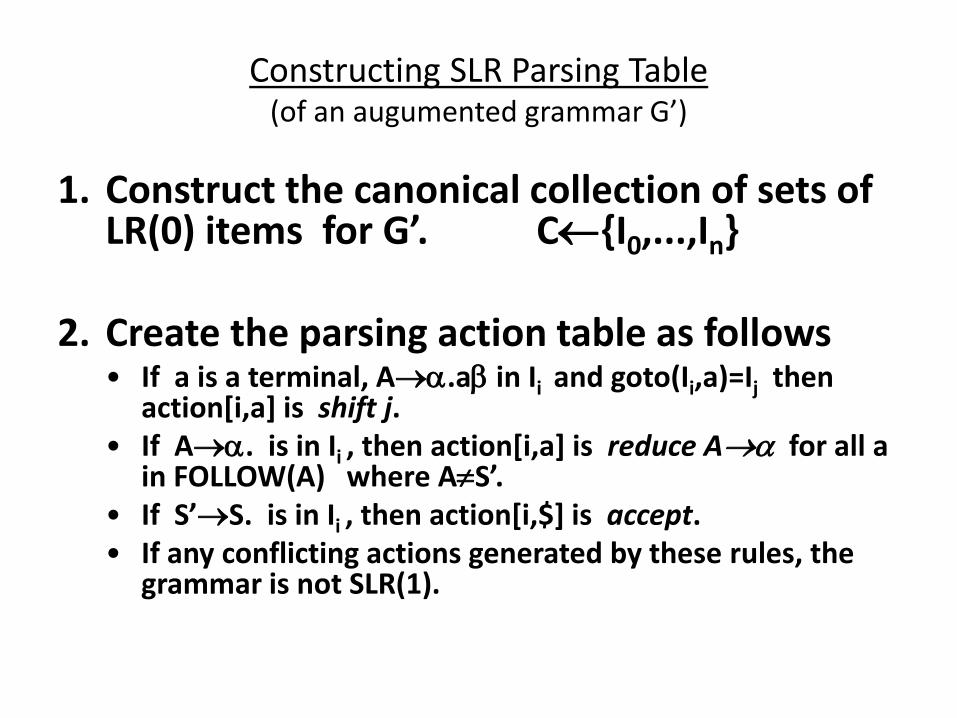
Constructing SLR Parsing Table of a augu e ted gra ar G’

1. Construct the canonical collection of sets of L‘ ite s fo G . C{I0,...,In}

2. Create the parsing action table as follows • If a is a terminal, A.a in Ii and goto(Ii,a)=Ij then

action[i,a] is shift j.

• If A. is in Ii , then action[i,a] is reduce A for all a in FOLLOW(A) where A“ .

• If “ S. is in Ii , then action[i,$] is accept.

• If any conflicting actions generated by these rules, the grammar is not SLR(1).

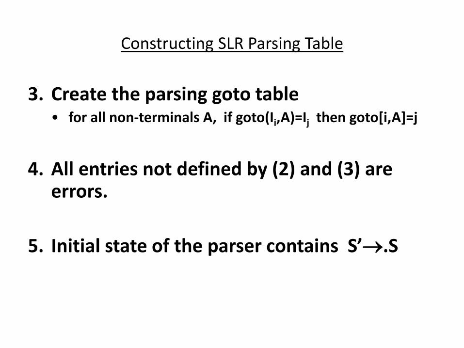
Constructing SLR Parsing Table

3. Create the parsing goto table • for all non-terminals A, if goto(Ii,A)=Ij then goto[i,A]=j

4. All entries not defined by (2) and (3) are errors.

5. I itial state of the pa se o tai s “ .S

Parsing Tables of Expression Grammar

state id + * ( ) $ E T F

0 s5 s4 1 2 3

1 s6 acc

2 r2 s7 r2 r2

3 r4 r4 r4 r4

4 s5 s4 8 2 3

5 r6 r6 r6 r6

6 s5 s4 9 3

7 s5 s4 10

8 s6 s11

9 r1 s7 r1 r1

10 r3 r3 r3 r3

11 r5 r5 r5 r5

Action Table Goto Table

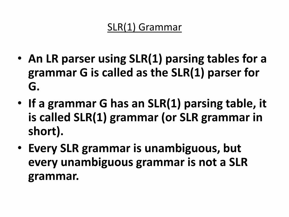
SLR(1) Grammar

• An LR parser using SLR(1) parsing tables for a grammar G is called as the SLR(1) parser for G.

• If a grammar G has an SLR(1) parsing table, it is called SLR(1) grammar (or SLR grammar in short).

• Every SLR grammar is unambiguous, but every unambiguous grammar is not a SLR grammar.

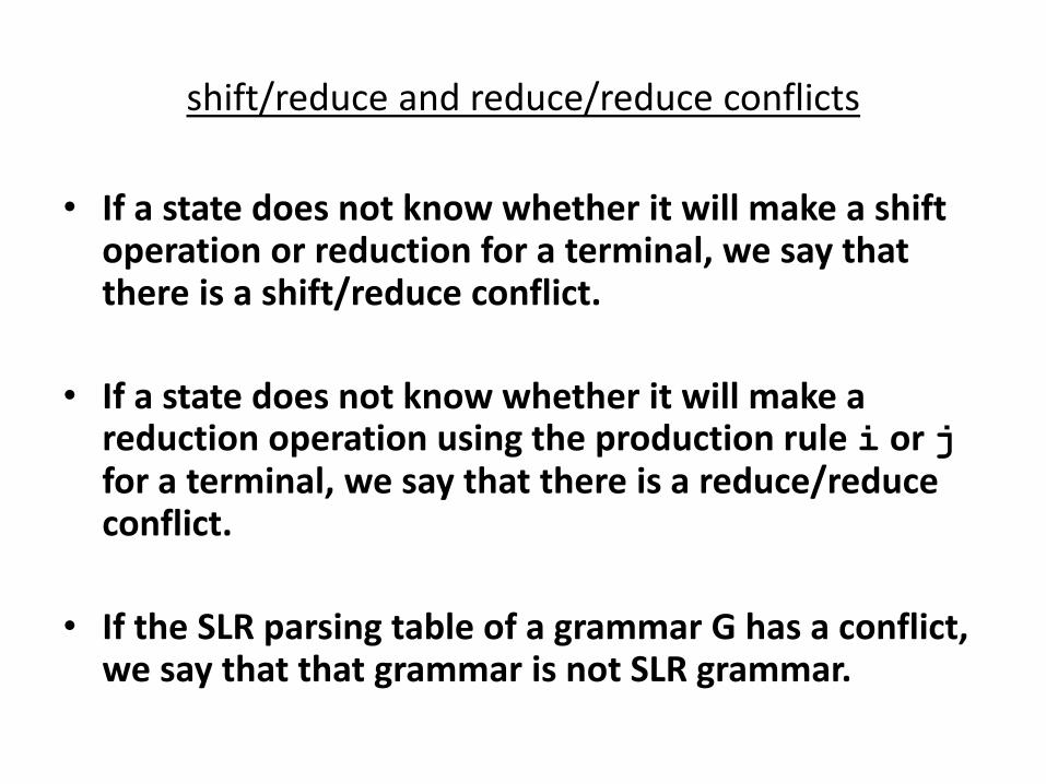
shift/reduce and reduce/reduce conflicts

• If a state does not know whether it will make a shift operation or reduction for a terminal, we say that there is a shift/reduce conflict.

• If a state does not know whether it will make a reduction operation using the production rule i or j for a terminal, we say that there is a reduce/reduce conflict.

• If the SLR parsing table of a grammar G has a conflict, we say that that grammar is not SLR grammar.

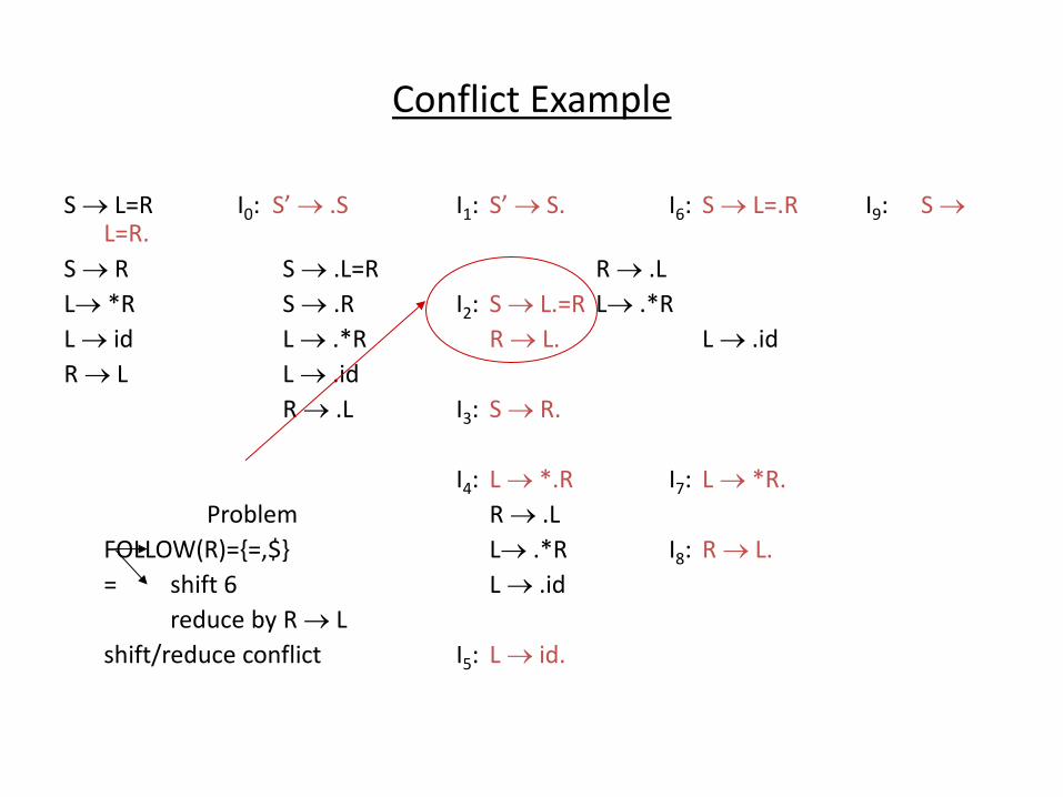
Conflict Example

S L=R I0: “’ .S I1: “’ S. I6: S L=.R I9: S L=R.

S R S .L=R R .L

L *R S .R I2: S L.=R L .*R

L id L .*R R L. L .id

R L L .id

R .L I3: S R.

I4: L *.R I7: L *R.

Problem R .L

FOLLOW(R)={=,$} L .*R I8: R L.

= shift 6 L .id

reduce by R L

shift/reduce conflict I5: L id.

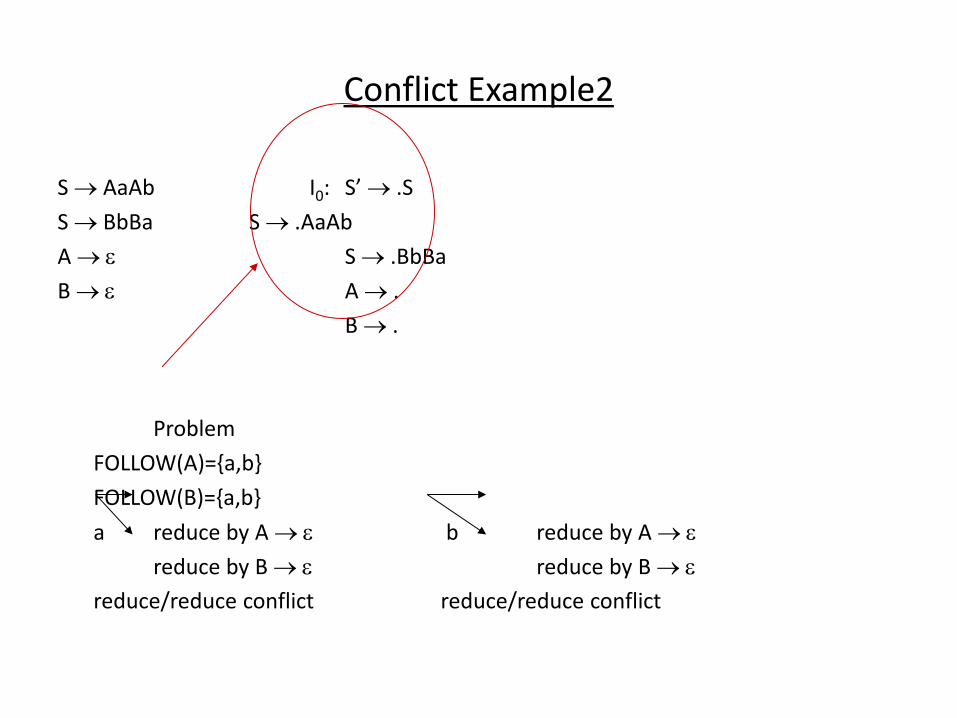
Conflict Example2

S AaAb I0: “’ .S

S BbBa S .AaAb

A S .BbBa

B A .

B .

Problem

FOLLOW(A)={a,b}

FOLLOW(B)={a,b}

a reduce by A b reduce by A

reduce by B reduce by B

reduce/reduce conflict reduce/reduce conflict

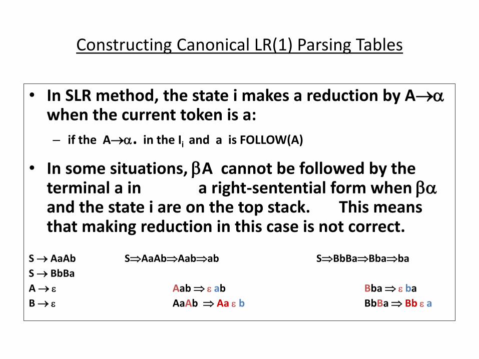
Constructing Canonical LR(1) Parsing Tables

• In SLR method, the state i makes a reduction by A when the current token is a:

– if the A. in the Ii and a is FOLLOW(A)

• In some situations, A cannot be followed by the terminal a in a right-sentential form when and the state i are on the top stack. This means that making reduction in this case is not correct.

S AaAb SAaAbAabab SBbBaBbaba

S BbBa

A Aab ab Bba ba

B AaAb Aa b BbBa Bb a

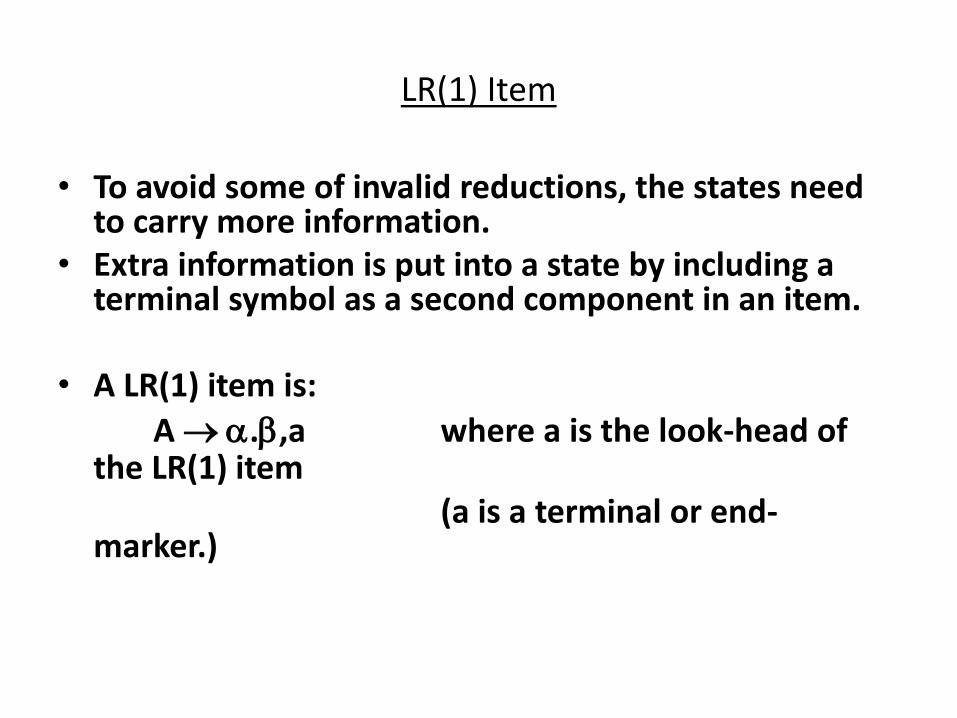
LR(1) Item

• To avoid some of invalid reductions, the states need to carry more information.

• Extra information is put into a state by including a terminal symbol as a second component in an item.

• A LR(1) item is:

A .,a where a is the look-head of the LR(1) item

(a is a terminal or end-marker.)

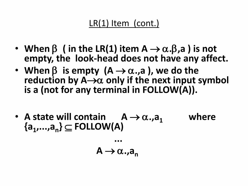
LR(1) Item (cont.)

• When ( in the LR(1) item A .,a ) is not empty, the look-head does not have any affect.

• When is empty (A .,a ), we do the reduction by A only if the next input symbol is a (not for any terminal in FOLLOW(A)).

• A state will contain A .,a1 where {a1,...,an} FOLLOW(A)

...

A .,an

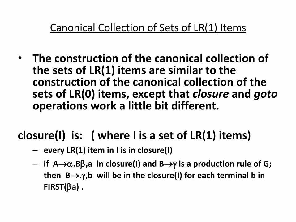
Canonical Collection of Sets of LR(1) Items

• The construction of the canonical collection of the sets of LR(1) items are similar to the construction of the canonical collection of the sets of LR(0) items, except that closure and goto operations work a little bit different.

closure(I) is: ( where I is a set of LR(1) items) – every LR(1) item in I is in closure(I)

– if A.B,a in closure(I) and B is a production rule of G;

then B.,b will be in the closure(I) for each terminal b in

FIRST(a) .

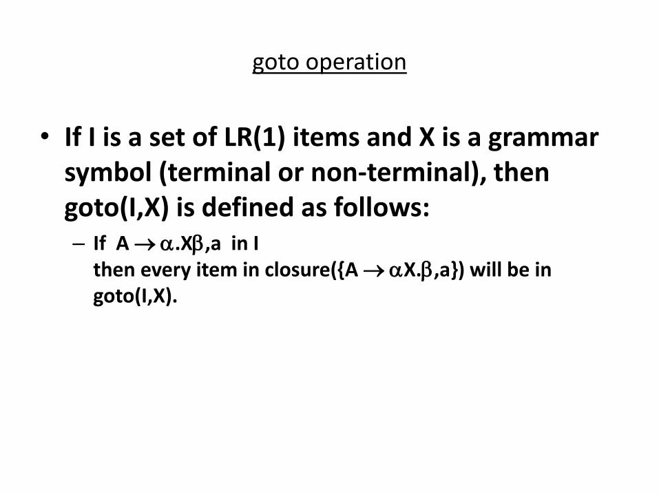
goto operation

• If I is a set of LR(1) items and X is a grammar

symbol (terminal or non-terminal), then

goto(I,X) is defined as follows: – If A .X,a in I

then every item in closure({A X.,a}) will be in

goto(I,X).

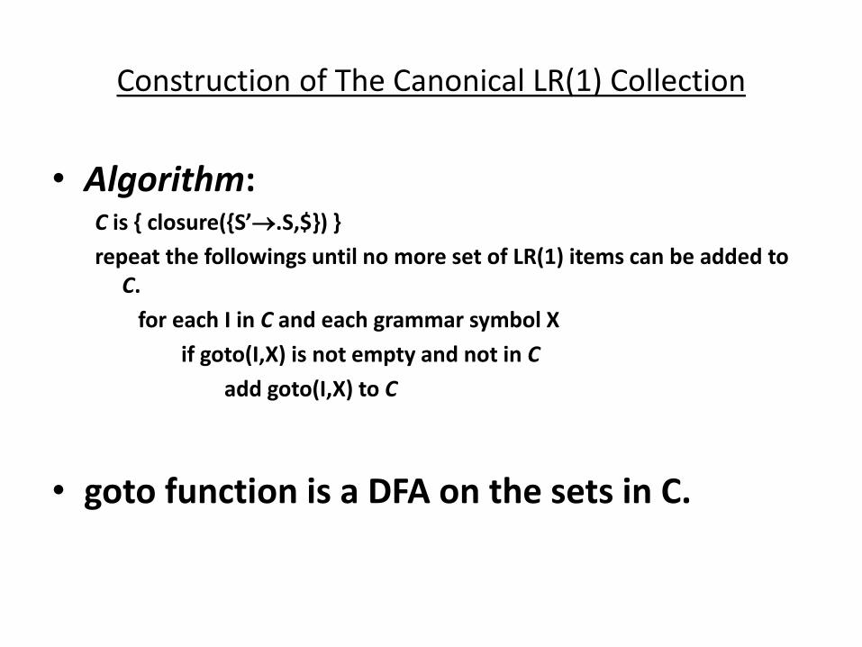
Construction of The Canonical LR(1) Collection

• Algorithm: C is { losu e {“ .S,$}) }

repeat the followings until no more set of LR(1) items can be added to

C.

for each I in C and each grammar symbol X

if goto(I,X) is not empty and not in C

add goto(I,X) to C

• goto function is a DFA on the sets in C.

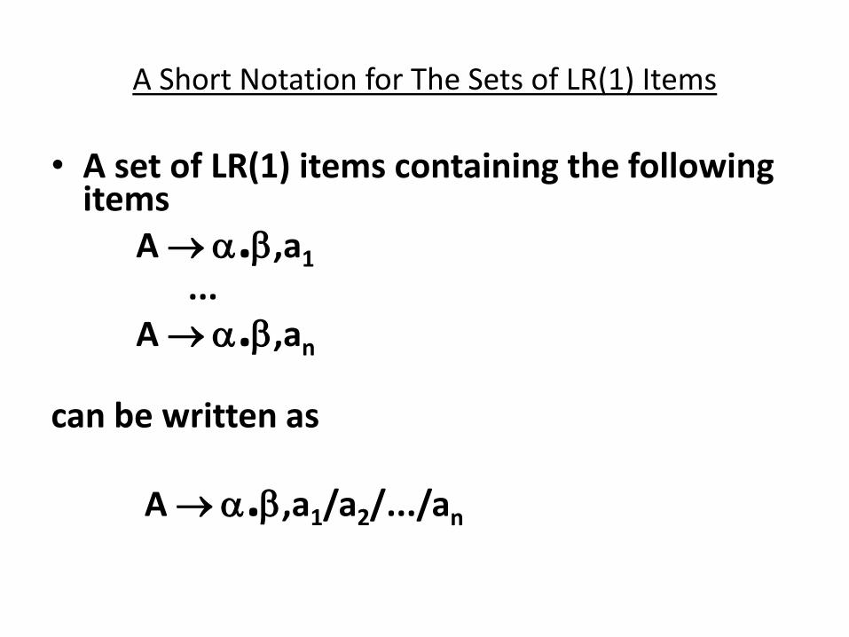
A Short Notation for The Sets of LR(1) Items

• A set of LR(1) items containing the following items

A .,a1

...

A .,an

can be written as

A .,a1/a2/.../an

Canonical LR(1) Collection -- Example

S AaAb I0: “’ .S ,$ I1: “’ S. ,$

S BbBa S .AaAb ,$

A S .BbBa ,$ I2: S A.aAb ,$

B A . ,a

B . ,b I3: S B.bBa ,$

I4: S Aa.Ab ,$ I6: S AaA.b ,$ I8: S AaAb. ,$

A . ,b

I5: S Bb.Ba ,$ I7: S BbB.a ,$ I9: S BbBa. ,$

B . ,a

S

A

B

a

b

A

B

a

b

to I4

to I5

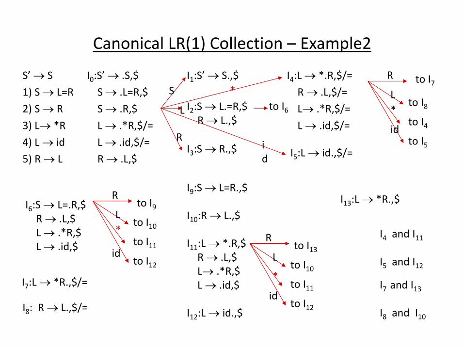
Canonical LR(1) Collection – Example2

“’ S

1) S L=R

2) S R

3) L *R

4) L id

5) R L

I0:“’ .S,$

S .L=R,$

S .R,$

L .*R,$/=

L .id,$/=

R .L,$

I1:“’ S.,$

I2:S L.=R,$

R L.,$

I3:S R.,$

I4:L *.R,$/=

R .L,$/=

L .*R,$/=

L .id,$/=

I5:L id.,$/=

I6:S L=.R,$

R .L,$

L .*R,$

L .id,$

I7:L *R.,$/=

I8: R L.,$/=

I9:S L=R.,$

I10:R L.,$

I11:L *.R,$

R .L,$

L .*R,$

L .id,$

I12:L id.,$

I13:L *R.,$

to I6

to I7

to I8

to I4

to I5

to I10

to I11

to I12

to I9

to I10

to I11

to I12

to I13

id

S

L

L

L

R

R

R

id

id

i

d

R

L

*

*

*

*

I4 and I11

I5 and I12

I7 and I13

I8 and I10

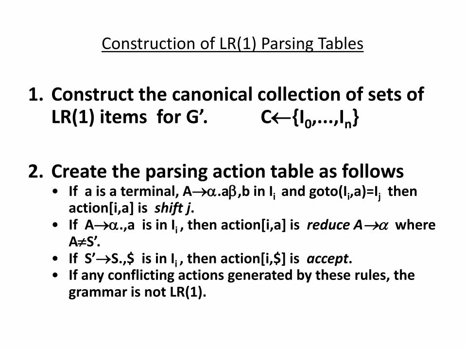
Construction of LR(1) Parsing Tables

1. Construct the canonical collection of sets of L‘ ite s fo G . C{I0,...,In}

2. Create the parsing action table as follows • If a is a terminal, A.a,b in Ii and goto(Ii,a)=Ij then

action[i,a] is shift j. • If A.,a is in Ii , then action[i,a] is reduce A where

A“ . • If “ S.,$ is in Ii , then action[i,$] is accept. • If any conflicting actions generated by these rules, the

grammar is not LR(1).

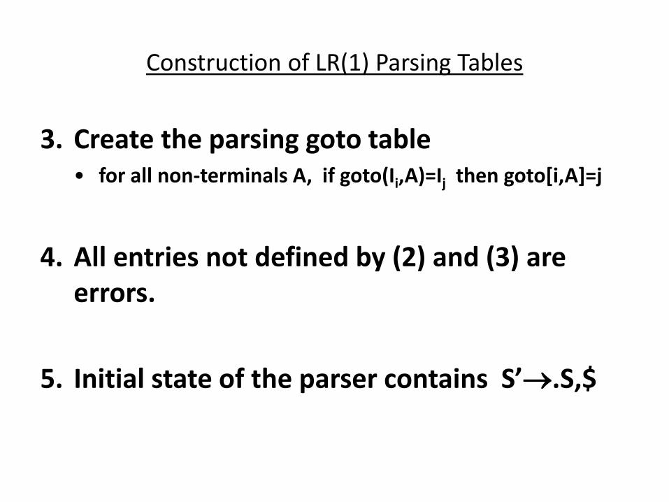
Construction of LR(1) Parsing Tables

3. Create the parsing goto table • for all non-terminals A, if goto(Ii,A)=Ij then goto[i,A]=j

4. All entries not defined by (2) and (3) are

errors.

5. I itial state of the pa se o tai s “ .S,$

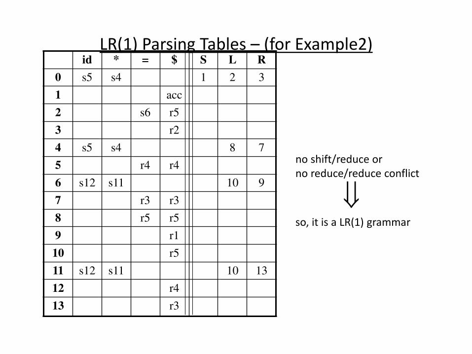
LR(1) Parsing Tables – (for Example2) id * = $ S L R

0 s5 s4 1 2 3

1 acc

2 s6 r5

3 r2

4 s5 s4 8 7

5 r4 r4

6 s12 s11 10 9

7 r3 r3

8 r5 r5

9 r1

10 r5

11 s12 s11 10 13

12 r4

13 r3

no shift/reduce or

no reduce/reduce conflict

so, it is a LR(1) grammar

LALR Parsing Tables

• LALR stands for LookAhead LR.

• LALR parsers are often used in practice because LALR parsing tables are smaller than LR(1) parsing tables.

• The number of states in SLR and LALR parsing tables for a grammar G are equal.

• But LALR parsers recognize more grammars than SLR parsers.

• yacc creates a LALR parser for the given grammar.

• A state of LALR parser will be again a set of LR(1) items.

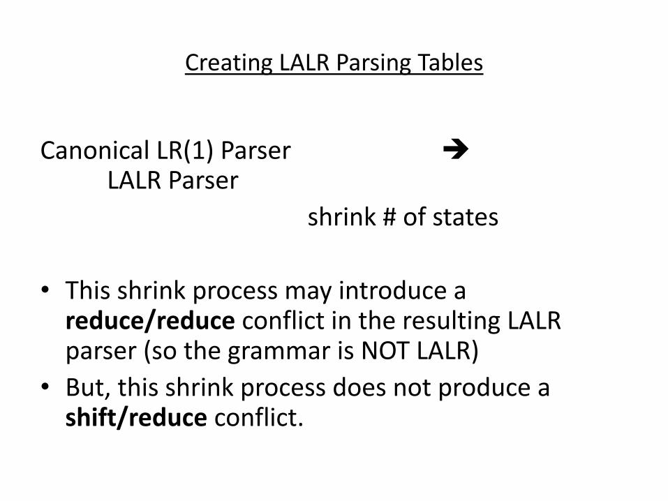
Creating LALR Parsing Tables

Canonical LR(1) Parser LALR Parser

shrink # of states

• This shrink process may introduce a reduce/reduce conflict in the resulting LALR parser (so the grammar is NOT LALR)

• But, this shrink process does not produce a shift/reduce conflict.

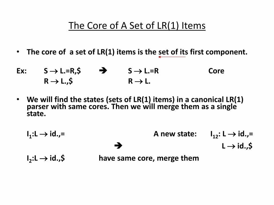
The Core of A Set of LR(1) Items

• The core of a set of LR(1) items is the set of its first component.

Ex: S L.=R,$ S L.=R Core

R L.,$ R L. • We will find the states (sets of LR(1) items) in a canonical LR(1)

parser with same cores. Then we will merge them as a single state.

I1:L id.,= A new state: I12: L id.,=

L id.,$

I2:L id.,$ have same core, merge them

The Core of A Set of LR(1) Items

• We will do this for all states of a canonical LR(1) parser to get the states of the LALR parser.

• In fact, the number of the states of the LALR parser for a grammar will be equal to the number of states of the SLR parser for that grammar.

Creation of LALR Parsing Tables

• Create the canonical LR(1) collection of the sets of LR(1) items for the given grammar.

• Find each core; find all sets having that same core; replace those sets having same cores with a single set which is their union.

C={I0,...,In} C ={J1,...,Jm} where m n • Create the parsing tables (action and goto tables) same as

the construction of the parsing tables of LR(1) parser. – Note that: If J=I1 ... Ik since I1,...,Ik have same cores cores of goto(I1,X),...,goto(I2,X) must be same. – So, goto(J,X)=K where K is the union of all sets of items having same

cores as goto(I1,X).

• If no conflict is introduced, the grammar is LALR(1) grammar. (We may only introduce reduce/reduce conflicts; we cannot introduce a shift/reduce conflict)

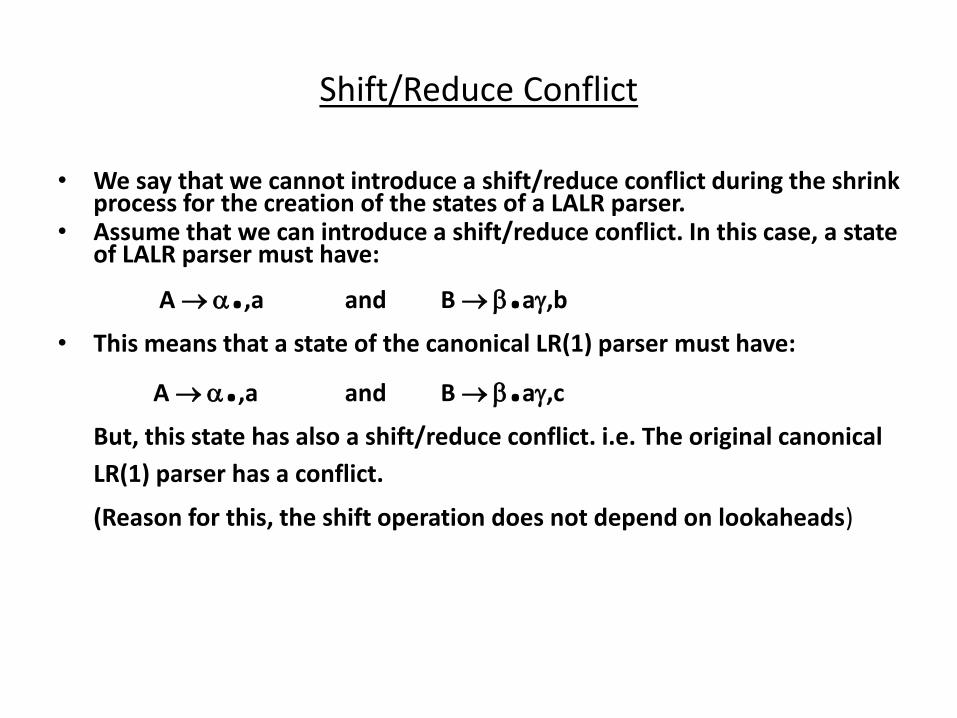
Shift/Reduce Conflict

• We say that we cannot introduce a shift/reduce conflict during the shrink process for the creation of the states of a LALR parser.

• Assume that we can introduce a shift/reduce conflict. In this case, a state of LALR parser must have:

A .,a and B .a,b

• This means that a state of the canonical LR(1) parser must have:

A .,a and B .a,c

But, this state has also a shift/reduce conflict. i.e. The original canonical

LR(1) parser has a conflict.

(Reason for this, the shift operation does not depend on lookaheads)

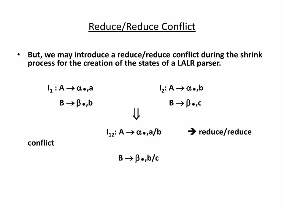
Reduce/Reduce Conflict

• But, we may introduce a reduce/reduce conflict during the shrink process for the creation of the states of a LALR parser.

I1 : A .,a I2: A .,b

B .,b B .,c

I12: A .,a/b reduce/reduce

conflict

B .,b/c

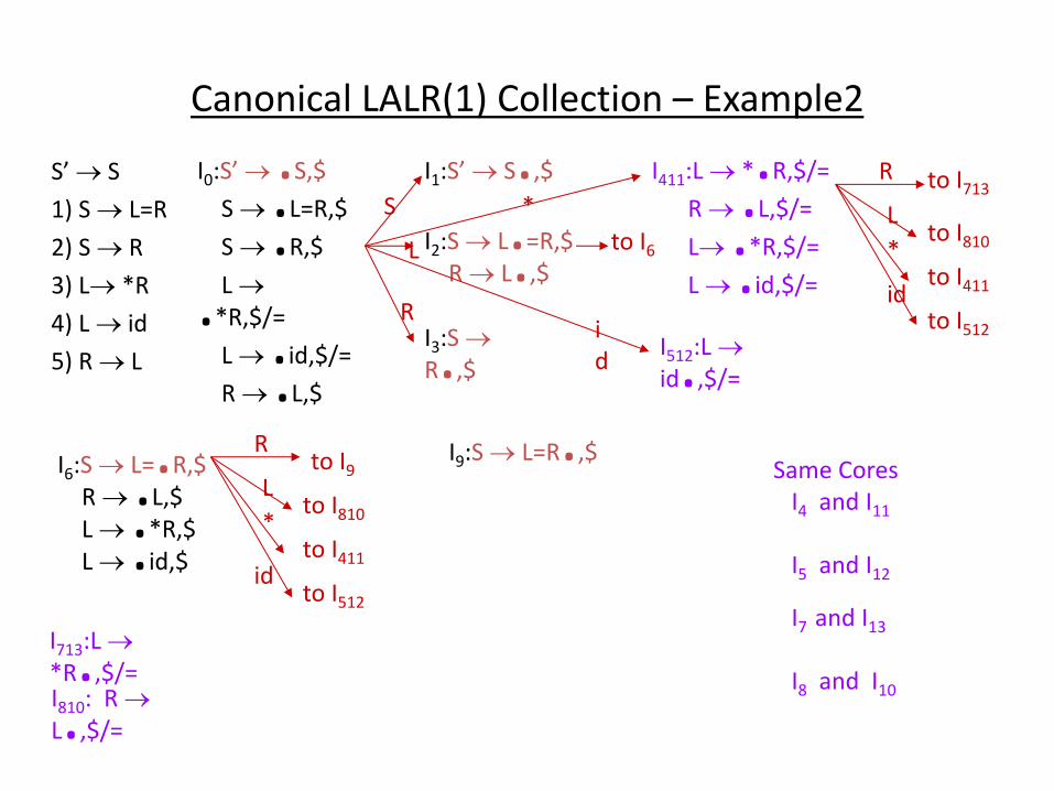
Canonical LALR(1) Collection – Example2

“’ S

1) S L=R

2) S R

3) L *R

4) L id

5) R L

I0:“’ .S,$

S .L=R,$

S .R,$

L .*R,$/=

L .id,$/=

R .L,$

I1:“’ S.,$

I2:S L.=R,$

R L.,$

I3:S

R.,$

I411:L *.R,$/=

R .L,$/=

L .*R,$/=

L .id,$/=

I512:L

id.,$/=

I6:S L=.R,$

R .L,$

L .*R,$

L .id,$

I713:L

*R.,$/= I810: R

L.,$/=

I9:S L=R.,$

to I6

to I713

to I810

to I411

to I512

to I810

to I411

to I512

to I9

S

L

L

L

R

R

id

id

i

d

R

*

*

*

Same Cores

I4 and I11

I5 and I12

I7 and I13

I8 and I10

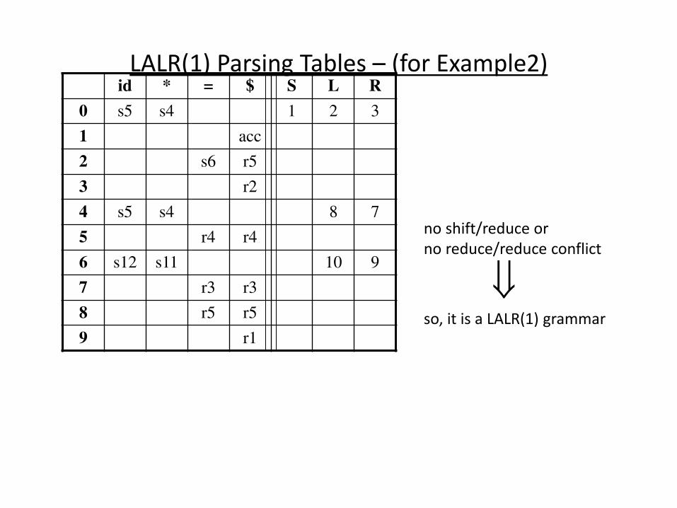
LALR(1) Parsing Tables – (for Example2) id * = $ S L R

0 s5 s4 1 2 3

1 acc

2 s6 r5

3 r2

4 s5 s4 8 7

5 r4 r4

6 s12 s11 10 9

7 r3 r3

8 r5 r5

9 r1

no shift/reduce or

no reduce/reduce conflict

so, it is a LALR(1) grammar

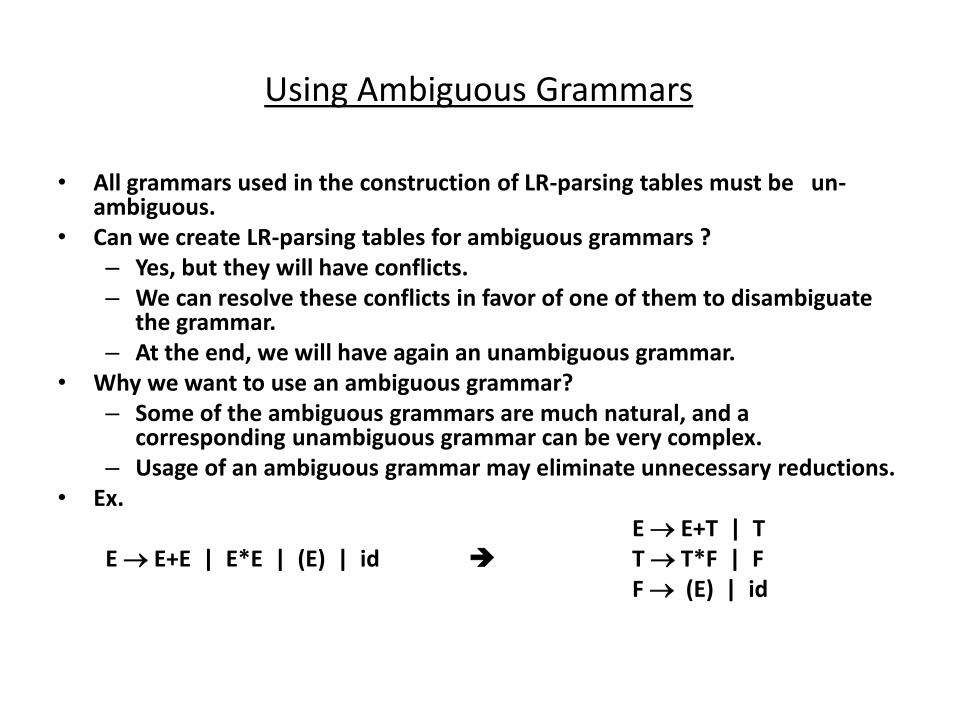
Using Ambiguous Grammars

• All grammars used in the construction of LR-parsing tables must be un-ambiguous.

• Can we create LR-parsing tables for ambiguous grammars ?

– Yes, but they will have conflicts.

– We can resolve these conflicts in favor of one of them to disambiguate the grammar.

– At the end, we will have again an unambiguous grammar.

• Why we want to use an ambiguous grammar?

– Some of the ambiguous grammars are much natural, and a corresponding unambiguous grammar can be very complex.

– Usage of an ambiguous grammar may eliminate unnecessary reductions.

• Ex.

E E+T | T

E E+E | E*E | (E) | id T T*F | F

F (E) | id

Sets of LR(0) Items for Ambiguous Grammar

I0: E’ .E

E .E+E

E .E*E

E .(E)

E .id

I1: E’ E. E E .+E

E E .*E

I2: E (.E)

E .E+E

E .E*E

E .(E)

E .id

I3: E id.

I4: E E +.E

E .E+E

E .E*E

E .(E)

E .id

I5: E E *.E

E .E+E

E .E*E

E .(E)

E .id

I6: E (E.)

E E.+E

E E.*E

I7: E E+E. E E.+E

E E.*E

I8: E E*E. E E.+E

E E.*E

I9: E (E).

I5

)

E

E

E

E

*

+

+

+

+

*

*

*

(

(

( (

id

id

id id

I4

I2

I2

I3

I3

I4

I4

I5

I5

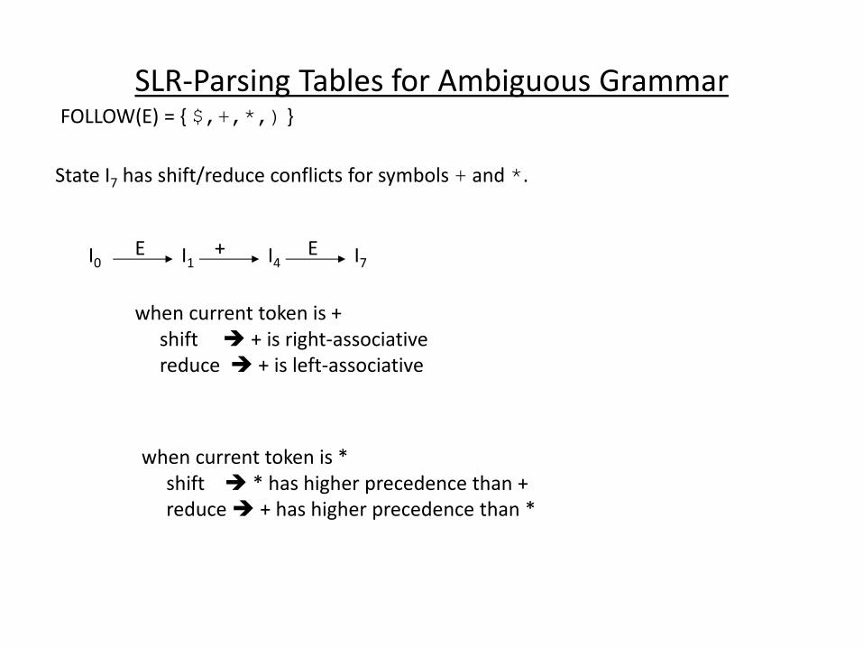
SLR-Parsing Tables for Ambiguous Grammar FOLLOW(E) = { $,+,*,) }

State I7 has shift/reduce conflicts for symbols + and *.

I0 I1 I7 I4 E + E

when current token is +

shift + is right-associative

reduce + is left-associative

when current token is *

shift * has higher precedence than +

reduce + has higher precedence than *

SLR-Parsing Tables for Ambiguous Grammar FOLLOW(E) = { $,+,*,) }

State I8 has shift/reduce conflicts for symbols + and *.

I0 I1 I7 I5 E * E

when current token is *

shift * is right-associative

reduce * is left-associative

when current token is +

shift + has higher precedence than *

reduce * has higher precedence than +

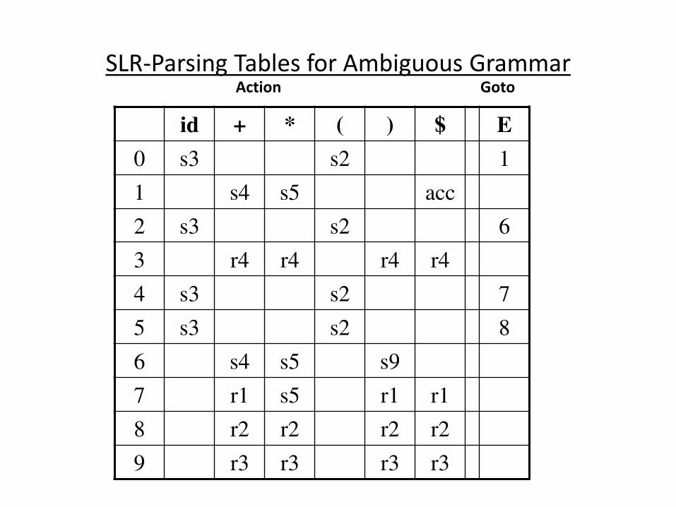
SLR-Parsing Tables for Ambiguous Grammar

id + * ( ) $ E

0 s3 s2 1

1 s4 s5 acc

2 s3 s2 6

3 r4 r4 r4 r4

4 s3 s2 7

5 s3 s2 8

6 s4 s5 s9

7 r1 s5 r1 r1

8 r2 r2 r2 r2

9 r3 r3 r3 r3

Action Goto

Error Recovery in LR Parsing

• An LR parser will detect an error when it consults the parsing action table and finds an error entry. All empty entries in the action table are error entries.

• Errors are never detected by consulting the goto table.

• An LR parser will announce error as soon as there is no valid continuation for the scanned portion of the input.

• A canonical LR parser (LR(1) parser) will never make even a single reduction before announcing an error.

• The SLR and LALR parsers may make several reductions before announcing an error.

• But, all LR parsers (LR(1), LALR and SLR parsers) will never shift an erroneous input symbol onto the stack.

Panic Mode Error Recovery in LR Parsing

• Scan down the stack until a state s with a goto on a particular nonterminal A is found. (Get rid of everything from the stack before this state s).

• Discard zero or more input symbols until a symbol a is found that can legitimately follow A. – The symbol a is simply in FOLLOW(A), but this may not work for all

situations.

• The parser stacks the nonterminal A and the state goto[s,A], and it resumes the normal parsing.

• This nonterminal A is normally is a basic programming block (there can be more than one choice for A). – stmt, expr, block, ...

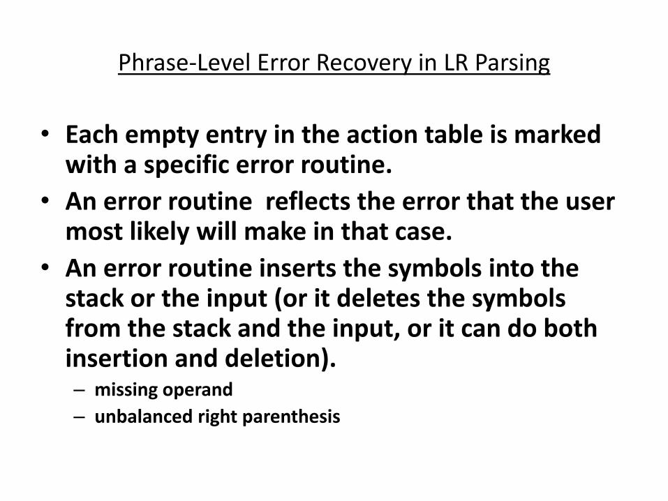
Phrase-Level Error Recovery in LR Parsing

• Each empty entry in the action table is marked with a specific error routine.

• An error routine reflects the error that the user most likely will make in that case.

• An error routine inserts the symbols into the stack or the input (or it deletes the symbols from the stack and the input, or it can do both insertion and deletion). – missing operand

– unbalanced right parenthesis

UNIT-3

PART-A

Semantic analysis

276

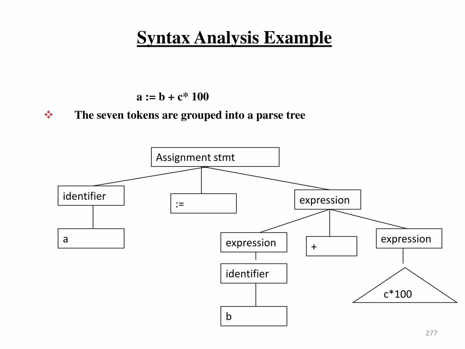
277

Syntax Analysis Example

a := b + c* 100

The seven tokens are grouped into a parse tree

Assignment stmt

identifier

a

:= expression

expression expression +

identifier

b

c*100

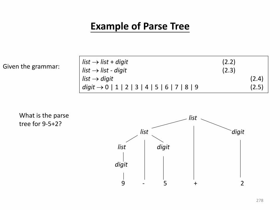
Example of Parse Tree

278

Given the grammar: list list + digit (2.2)

list list - digit (2.3)

list digit (2.4)

digit 0 | 1 | 2 | 3 | 4 | 5 | 6 | 7 | 8 | 9 (2.5)

What is the parse

tree for 9-5+2? list

digit

list digit

list digit

9 - 5 + 2

Abstract Syntax Tree (AST)

279

The AST is a condensed/simplified/abstract form of

the parse tree in which:

1. Operators are directly associated with interior nodes

(non-terminals)

2. Chains of single productions are collapsed.

3. Terminals that have no attributes are ignored, i.e.,

the corresponding leaf nodes are discarded.

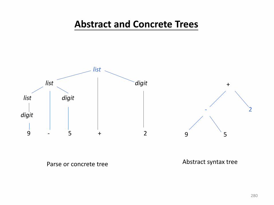
Abstract and Concrete Trees

280

list

digit

list digit

list digit

9 - 5 + 2

Parse or concrete tree

+

- 2

9 5

Abstract syntax tree

Advantages of the AST Representation

281

• Convenient representation for semantic analysis and

intermediate-language (IL) generation

• Useful for building other programming language tools e.t., a

syntax-directed editor

282

Syntax Directed Translation (SDT)

Syntax-directed translation is a method of translating a string into a

sequence of actions by attaching on such action to each rule of a grammar.

A syntax-directed translation is defined by augmenting the CFG: a translation

rule is defined for each production. A translation rule defines the translation

of the left-hand side non terminal.

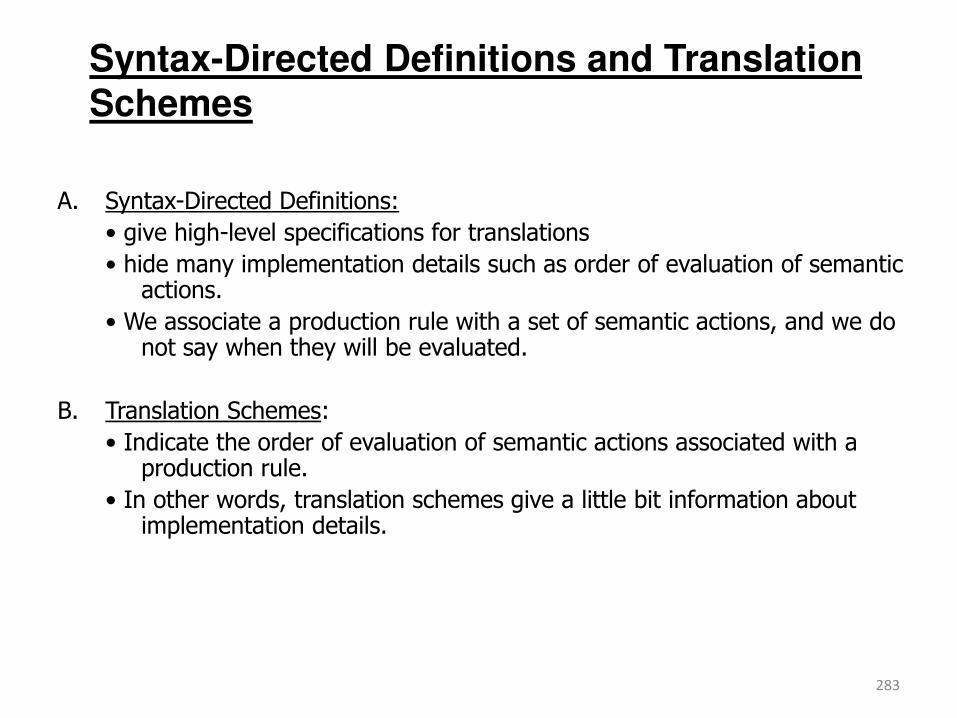
283

Syntax-Directed Definitions and Translation

Schemes

A. Syntax-Directed Definitions:

• give high-level specifications for translations

• hide many implementation details such as order of evaluation of semantic actions.

• We associate a production rule with a set of semantic actions, and we do not say when they will be evaluated.

B. Translation Schemes:

• Indicate the order of evaluation of semantic actions associated with a production rule.

• In other words, translation schemes give a little bit information about implementation details.

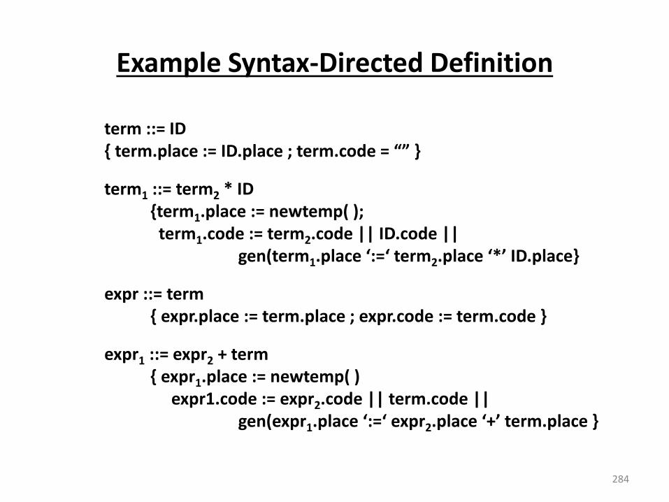
Example Syntax-Directed Definition

term ::= ID

{ te .pla e := ID.pla e ; te . ode = } term1 ::= term2 * ID

{term1.place := newtemp( );

term1.code := term2.code || ID.code ||

gen(term1.pla e := te 2.pla e * ID.pla e} expr ::= term

{ expr.place := term.place ; expr.code := term.code } expr1 ::= expr2 + term

{ expr1.place := newtemp( )

expr1.code := expr2.code || term.code ||

gen(expr1.pla e := e p 2.pla e + te .pla e }

284

285

YACC – Yet Another Compiler-Compiler

A bottom-up parser generator

It provides semantic stack manipulation and supports specification of semantic routines.

Developed by Steve Johnson and others at AT&T Bell Lab.

Can use scanner generated by Lex or hand-coded scanner in C

Used by many compilers and tools, including production compilers.

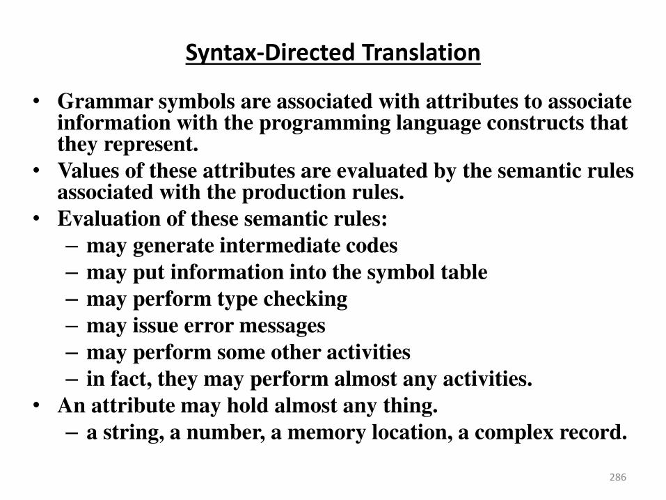
Syntax-Directed Translation

• Grammar symbols are associated with attributes to associate information with the programming language constructs that they represent.

• Values of these attributes are evaluated by the semantic rules associated with the production rules.

• Evaluation of these semantic rules:

– may generate intermediate codes

– may put information into the symbol table

– may perform type checking

– may issue error messages

– may perform some other activities

– in fact, they may perform almost any activities.

• An attribute may hold almost any thing.

– a string, a number, a memory location, a complex record.

286

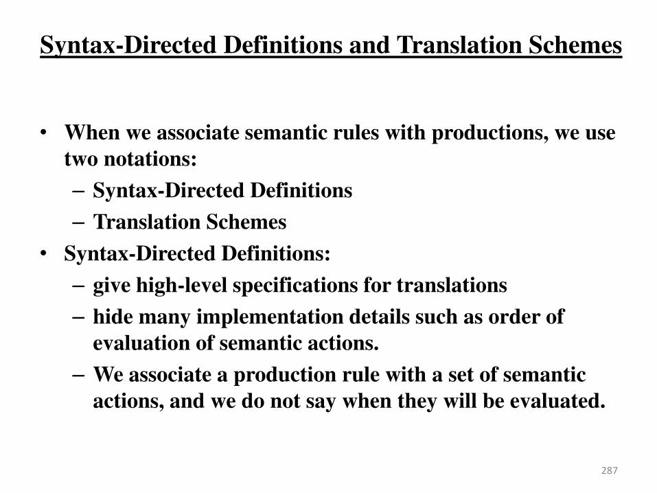
Syntax-Directed Definitions and Translation Schemes

287

• When we associate semantic rules with productions, we use

two notations:

– Syntax-Directed Definitions

– Translation Schemes

• Syntax-Directed Definitions:

– give high-level specifications for translations

– hide many implementation details such as order of

evaluation of semantic actions.

– We associate a production rule with a set of semantic

actions, and we do not say when they will be evaluated.

Syntax-Directed Definitions and Translation Schemes

• Translation Schemes:

– indicate the order of evaluation of semantic actions

associated with a production rule.

– In other words, translation schemes give a little bit

information about implementation details.

288

Syntax-Directed Definitions

• A syntax-directed definition is a generalization of a context-

free grammar in which:

– Each grammar symbol is associated with a set of attributes.

– This set of attributes for a grammar symbol is partitioned

into two subsets called synthesized and inherited attributes

of that grammar symbol.

– Each production rule is associated with a set of semantic

rules.

• Semantic rules set up dependencies between attributes which

can be represented by a dependency graph.

• This dependency graph determines the evaluation order of

these semantic rules.

• Evaluation of a semantic rule defines the value of an attribute.

But a semantic rule may also have some side effects such as

printing a value.

289

Annotated Parse Tree

• A parse tree showing the values of attributes at each node

is called an annotated parse tree.

• The process of computing the attributes values at the nodes

is called annotating (or decorating) of the parse tree.

• Of course, the order of these computations depends on the

dependency graph induced by the semantic rules.

290

Syntax-Directed Definition

• In a syntax-directed definition, each production A α is associated with a set of semantic rules of the form:

b=f(c1,c2,…,cn) where f is a function,

and b can be one of the followings:

b is a synthesized attribute of A and c1,c2,…,cn are attributes of the grammar symbols in the production ( A α ).

OR

b is an inherited attribute one of the grammar symbols in α (on the

right side of the production), and c1,c2,…,cn are attributes of the grammar symbols in the production ( A α ).

291

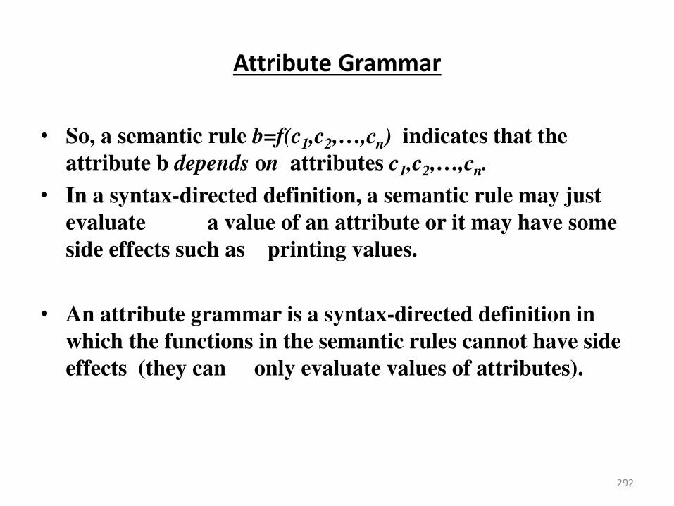
Attribute Grammar

• So, a semantic rule b=f(c1,c2,…,cn) indicates that the

attribute b depends on attributes c1,c2,…,cn.

• In a syntax-directed definition, a semantic rule may just

evaluate a value of an attribute or it may have some

side effects such as printing values.

• An attribute grammar is a syntax-directed definition in

which the functions in the semantic rules cannot have side

effects (they can only evaluate values of attributes).

292

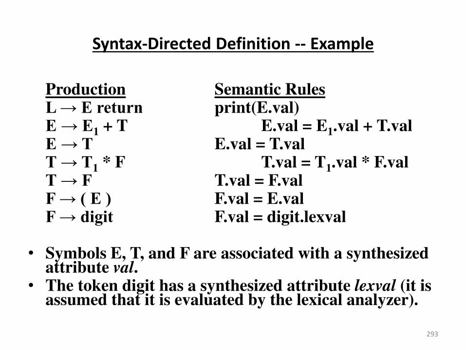
Syntax-Directed Definition -- Example

Production Semantic Rules L E return print(E.val) E E1 + T E.val = E1.val + T.val E T E.val = T.val T T1 * F T.val = T1.val * F.val T F T.val = F.val F ( E ) F.val = E.val F digit F.val = digit.lexval • Symbols E, T, and F are associated with a synthesized

attribute val. • The token digit has a synthesized attribute lexval (it is

assumed that it is evaluated by the lexical analyzer). 293

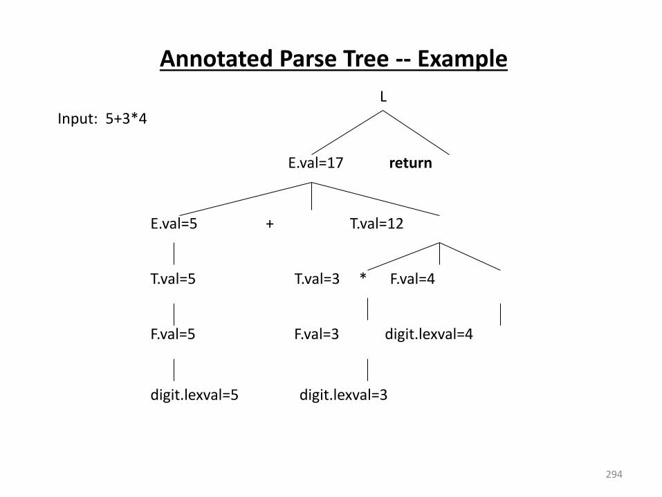
Annotated Parse Tree -- Example

294

Input: 5+3*4

L

E.val=17 return

E.val=5 + T.val=12

T.val=5 T.val=3 * F.val=4

F.val=5 F.val=3 digit.lexval=4

digit.lexval=5 digit.lexval=3

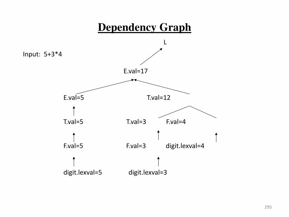
Dependency Graph

295

Input: 5+3*4

L

E.val=17

E.val=5 T.val=12

T.val=5 T.val=3 F.val=4

F.val=5 F.val=3 digit.lexval=4

digit.lexval=5 digit.lexval=3

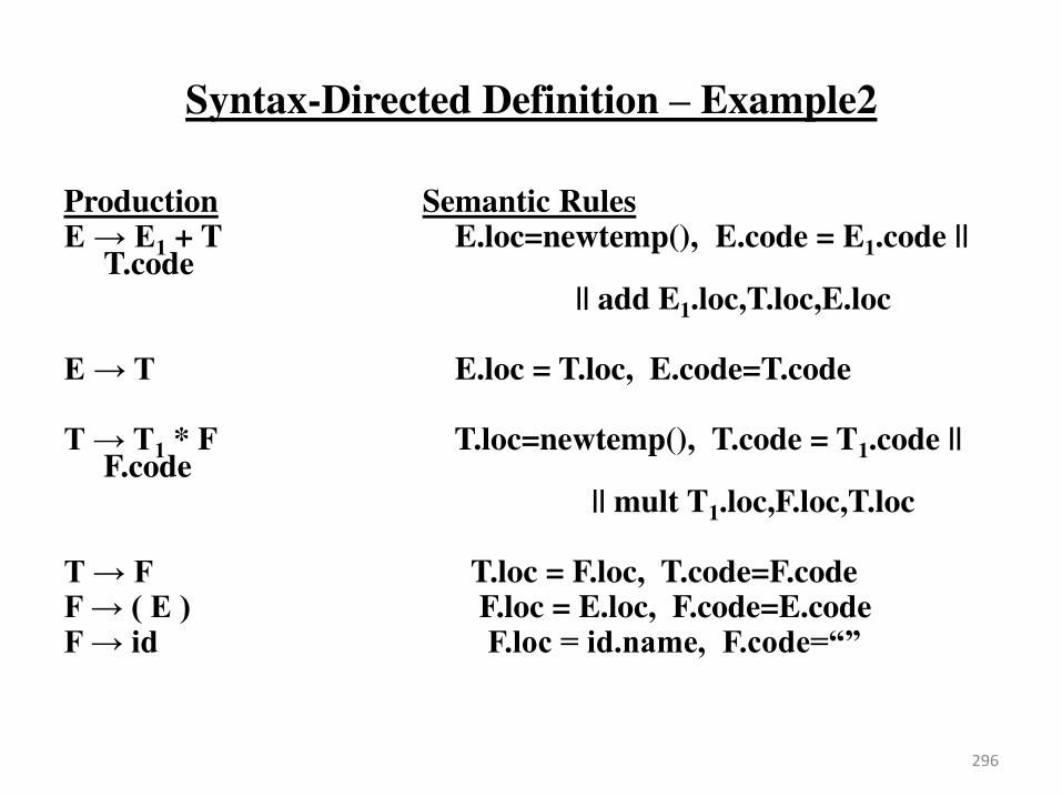
Syntax-Directed Definition – Example2

Production Semantic Rules E E1 + T E.loc=newtemp(), E.code = E1.code ||

T.code || add E1.loc,T.loc,E.loc E T E.loc = T.loc, E.code=T.code T T1 * F T.loc=newtemp(), T.code = T1.code ||

F.code || mult T1.loc,F.loc,T.loc T F T.loc = F.loc, T.code=F.code F ( E ) F.loc = E.loc, F.code=E.code F id F.loc = id.name, F.code=“”

296

Syntax-Directed Definition – Example2

• Symbols E, T, and F are associated with synthesized attributes loc and code.

• The token id has a synthesized attribute name (it is assumed that it is evaluated by the lexical analyzer).

• It is assumed that || is the string concatenation operator.

297

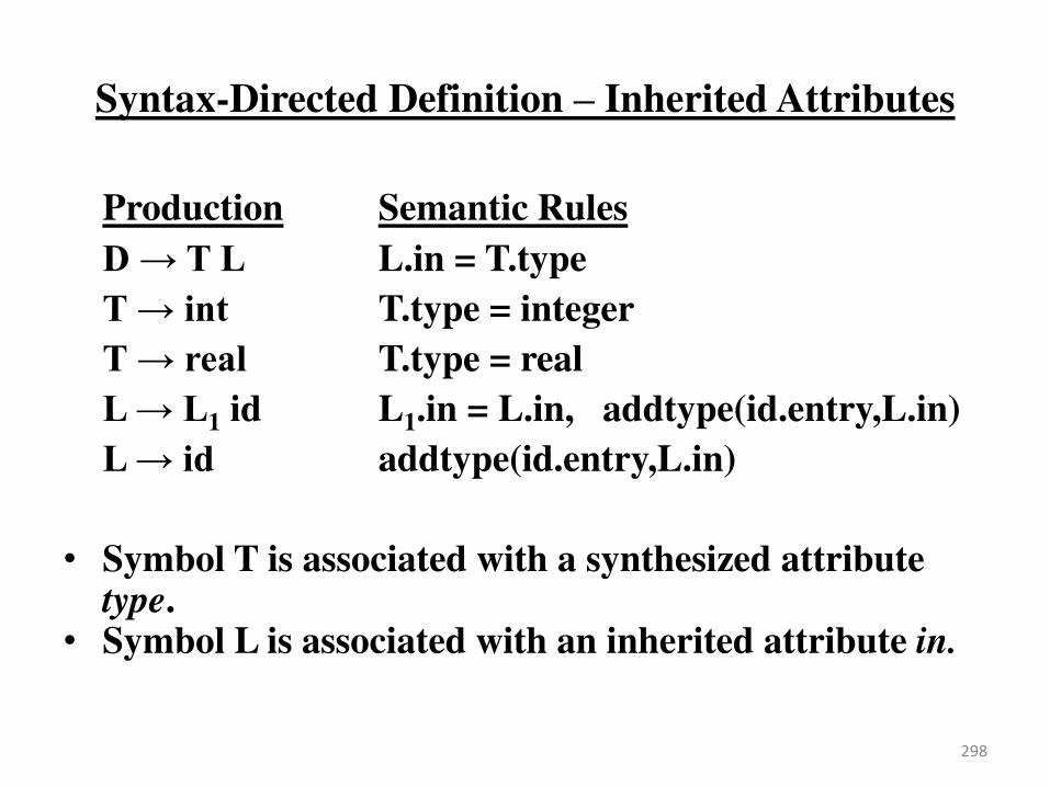
Syntax-Directed Definition – Inherited Attributes

Production Semantic Rules

D T L L.in = T.type

T int T.type = integer

T real T.type = real

L L1 id L1.in = L.in, addtype(id.entry,L.in)

L id addtype(id.entry,L.in)

• Symbol T is associated with a synthesized attribute type.

• Symbol L is associated with an inherited attribute in.

298

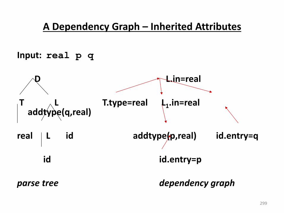
A Dependency Graph – Inherited Attributes

Input: real p q

D L.in=real

T L T.type=real L1.in=real addtype(q,real)

real L id addtype(p,real) id.entry=q

id id.entry=p

parse tree dependency graph

299

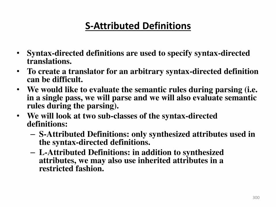
S-Attributed Definitions

• Syntax-directed definitions are used to specify syntax-directed translations.

• To create a translator for an arbitrary syntax-directed definition can be difficult.

• We would like to evaluate the semantic rules during parsing (i.e. in a single pass, we will parse and we will also evaluate semantic rules during the parsing).

• We will look at two sub-classes of the syntax-directed definitions:

– S-Attributed Definitions: only synthesized attributes used in the syntax-directed definitions.

– L-Attributed Definitions: in addition to synthesized attributes, we may also use inherited attributes in a restricted fashion.

300

S-Attributed Definitions

• To implement S-Attributed Definitions and L-Attributed

Definitions are easy (we can evaluate semantic rules in a

single pass during the parsing).

• Implementations of S-attributed Definitions are a little bit

easier than implementations of L-Attributed Definitions

301

Bottom-Up Evaluation of S-Attributed Definitions

• We put the values of the synthesized attributes of the

grammar symbols into a parallel stack.

– When an entry of the parser stack holds a grammar

symbol X (terminal or non-terminal), the

corresponding entry in the parallel stack will hold the

synthesized attribute(s) of the symbol X.

• We evaluate the values of the attributes during reductions.

302

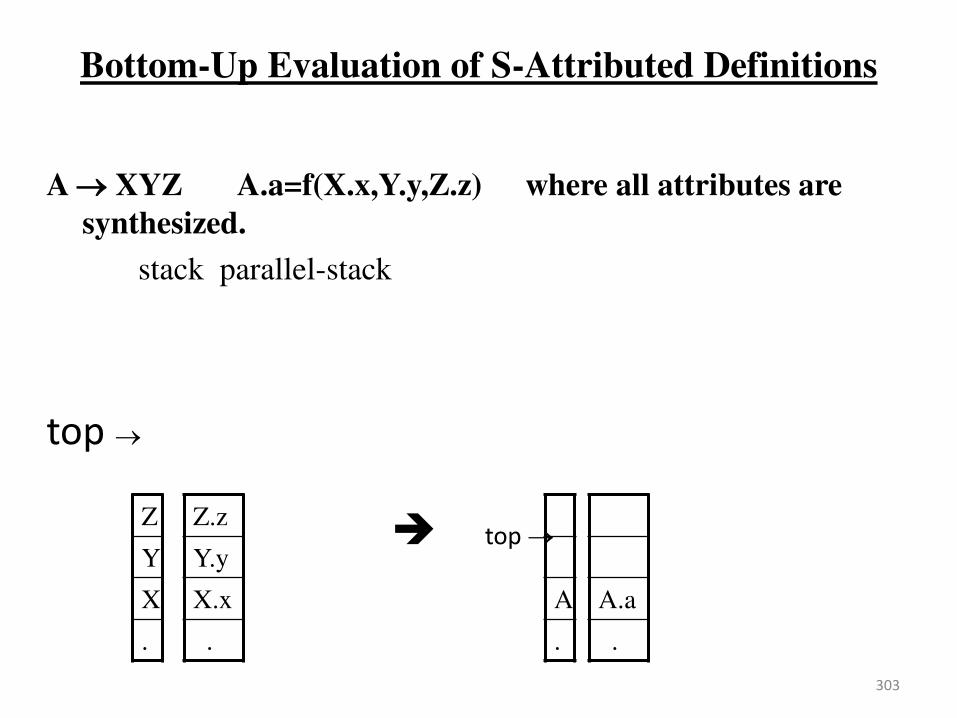
Bottom-Up Evaluation of S-Attributed Definitions

A XYZ A.a=f(X.x,Y.y,Z.z) where all attributes are

synthesized.

stack parallel-stack

top

top

303

Z

Y

X

.

Z.z

Y.y

X.x

.

A

.

A.a

.

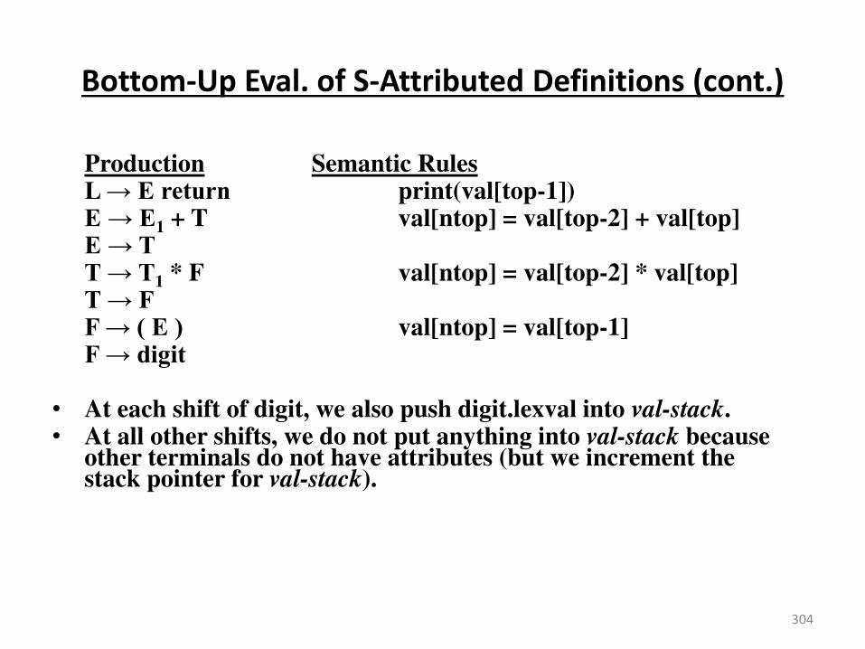
Bottom-Up Eval. of S-Attributed Definitions (cont.)

Production Semantic Rules L E return print(val[top-1]) E E1 + T val[ntop] = val[top-2] + val[top] E T T T1 * F val[ntop] = val[top-2] * val[top] T F F ( E ) val[ntop] = val[top-1] F digit • At each shift of digit, we also push digit.lexval into val-stack. • At all other shifts, we do not put anything into val-stack because

other terminals do not have attributes (but we increment the stack pointer for val-stack).

304

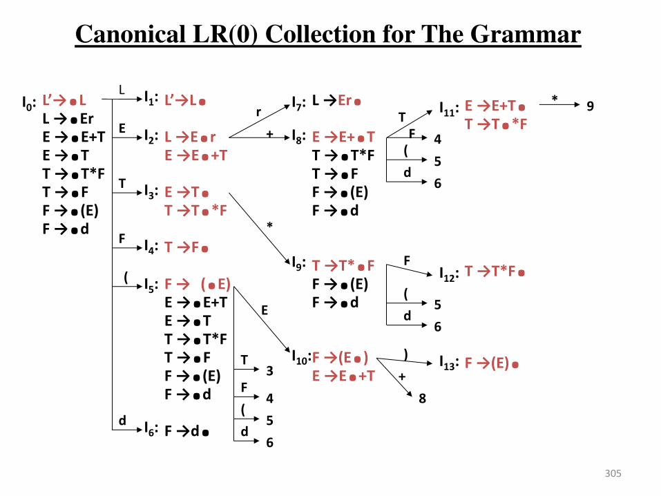
Canonical LR(0) Collection for The Grammar

305

L →.L L →.Er E →.E+T E →.T T →.T*F T →.F F →.(E) F →.d

L →L. L →E.r E →E.+T E →T. T →T.*F T →F. F → (.E) E →.E+T E →.T T →.T*F T →.F F →.(E) F →.d F →d.

L →Er. E →E+.T T →.T*F T →.F F →.(E) F →.d T →T*.F F →.(E) F →.d F → E.) E →E.+T

E →E+T. T →T.*F T →T*F. F → E .

I0: I1:

I2:

I4:

I3:

I5:

I6:

I7:

I12:

I11:

I10:

I9:

I13:

I8:

r

L

E

E T

T

T

F

F

F

F

(

(

( (

d

d

d d

)

*

+

+

*

6

3

5

4

6

6

5

5

8

9

4

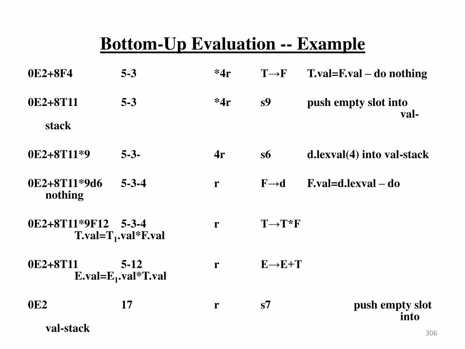
Bottom-Up Evaluation -- Example

0E2+8F4 5-3 *4r T F T.val=F.val – do nothing

0E2+8T11 5-3 *4r s9 push empty slot into val-stack

0E2+8T11*9 5-3- 4r s6 d.lexval(4) into val-stack

0E2+8T11*9d6 5-3-4 r F d F.val=d.lexval – do nothing

0E2+8T11*9F12 5-3-4 r T T*F T.val=T1.val*F.val

0E2+8T11 5-12 r E E+T E.val=E1.val*T.val

0E2 17 r s7 push empty slot into val-stack

L Er

306

Top-Down Evaluation (of S-Attributed Definitions)

Productions Semantic Rules

A B print(B.n0), print(B.n1)

B 0 B1 B.n0=B1.n0+1, B.n1=B1.n1

B 1 B1 B.n0=B1.n0, B.n1=B1.n1+1

B B.n0=0, B.n1=0

where B has two synthesized attributes (n0 and n1).

307

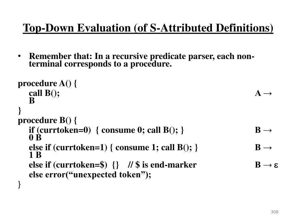
Top-Down Evaluation (of S-Attributed Definitions)

• Remember that: In a recursive predicate parser, each non-terminal corresponds to a procedure.

procedure A() { call B(); A

B } procedure B() { if (currtoken=0) { consume 0; call B(); } B

0 B else if (currtoken=1) { consume 1; call B(); } B

1 B else if (currtoken=$) {} // $ is end-marker B else error(“unexpected token”); }

308

Top-Down Evaluation (of S-Attributed Definitions)

procedure A() {

int n0,n1; Synthesized attributes of non-terminal B

call B(&n0,&n1); are the output parameters of procedure B.

print(n0); print(n1);

} All the semantic rules can be evaluated

procedure B(int *n0, int *n1) { at the end of parsing of production rules

if (currtoken=0)

{int a,b; consume 0; call B(&a,&b); *n0=a+1; *n1=b;}

else if (currtoken=1)

{ int a,b; consume 1; call B(&a,&b); *n0=a; *n1=b+1; }

else if (currtoken=$) {*n0=0; *n1=0; } // $ is end-marker

else error(“unexpected token”); }

309

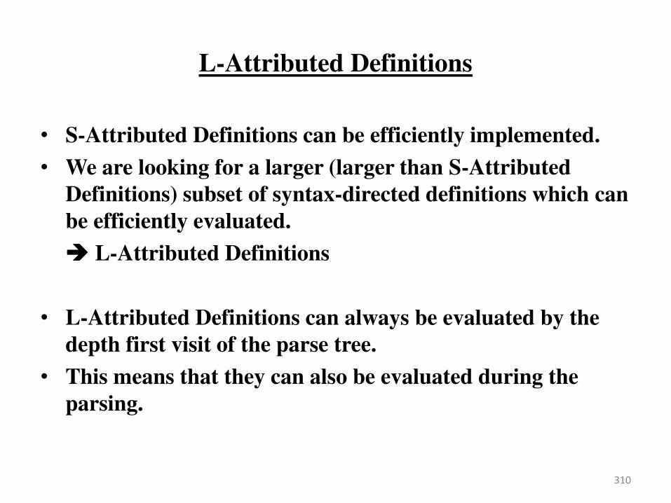
L-Attributed Definitions

• S-Attributed Definitions can be efficiently implemented.

• We are looking for a larger (larger than S-Attributed

Definitions) subset of syntax-directed definitions which can

be efficiently evaluated.

L-Attributed Definitions

• L-Attributed Definitions can always be evaluated by the

depth first visit of the parse tree.

• This means that they can also be evaluated during the

parsing.

310

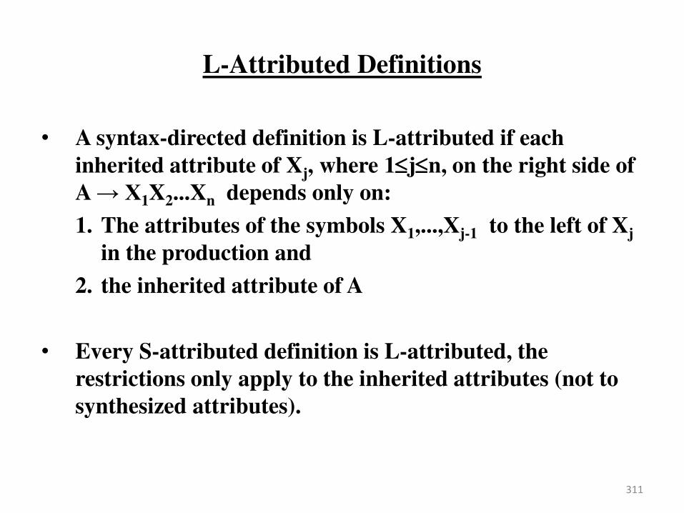
L-Attributed Definitions

• A syntax-directed definition is L-attributed if each

inherited attribute of Xj, where 1jn, on the right side of A X1X2...Xn depends only on:

1. The attributes of the symbols X1,...,Xj-1 to the left of Xj

in the production and

2. the inherited attribute of A

• Every S-attributed definition is L-attributed, the

restrictions only apply to the inherited attributes (not to

synthesized attributes).

311

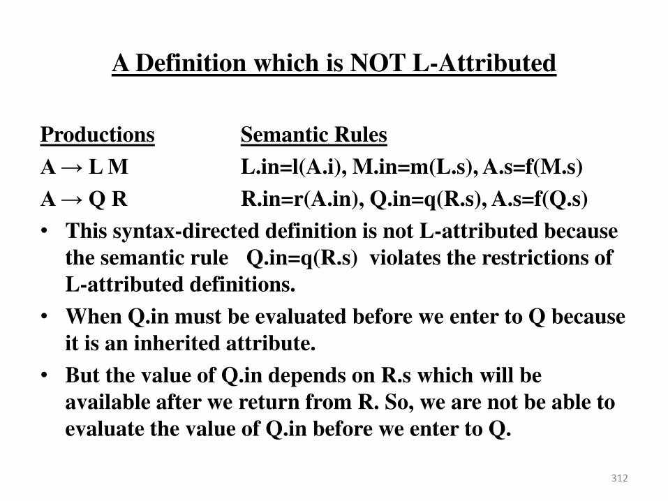
A Definition which is NOT L-Attributed

Productions Semantic Rules

A L M L.in=l(A.i), M.in=m(L.s), A.s=f(M.s)

A Q R R.in=r(A.in), Q.in=q(R.s), A.s=f(Q.s)

• This syntax-directed definition is not L-attributed because

the semantic rule Q.in=q(R.s) violates the restrictions of

L-attributed definitions.

• When Q.in must be evaluated before we enter to Q because

it is an inherited attribute.

• But the value of Q.in depends on R.s which will be

available after we return from R. So, we are not be able to

evaluate the value of Q.in before we enter to Q.

312

Translation Schemes

• In a syntax-directed definition, we do not say anything

about the evaluation times of the semantic rules (when the

semantic rules associated with a production should be

evaluated?).

• A translation scheme is a context-free grammar in which:

– attributes are associated with the grammar symbols and

– semantic actions enclosed between braces {} are

inserted within the right sides of productions.

• Ex: A { ... } X { ... } Y { ... }

Semantic Actions 313

Translation Schemes

• When designing a translation scheme, some restrictions

should be observed to ensure that an attribute value is

available when a semantic action refers to that attribute.

• These restrictions (motivated by L-attributed definitions)

ensure that a semantic action does not refer to an

attribute that has not yet computed.

• In translation schemes, we use semantic action

terminology instead of semantic rule terminology used in

syntax-directed definitions.

• The position of the semantic action on the right side

indicates when that semantic action will be evaluated.

314

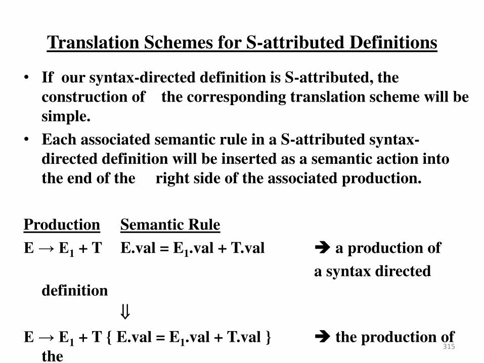
Translation Schemes for S-attributed Definitions

• If our syntax-directed definition is S-attributed, the

construction of the corresponding translation scheme will be

simple.

• Each associated semantic rule in a S-attributed syntax-

directed definition will be inserted as a semantic action into

the end of the right side of the associated production.

Production Semantic Rule

E E1 + T E.val = E1.val + T.val a production of

a syntax directed

definition

E E1 + T { E.val = E1.val + T.val } the production of

the 315

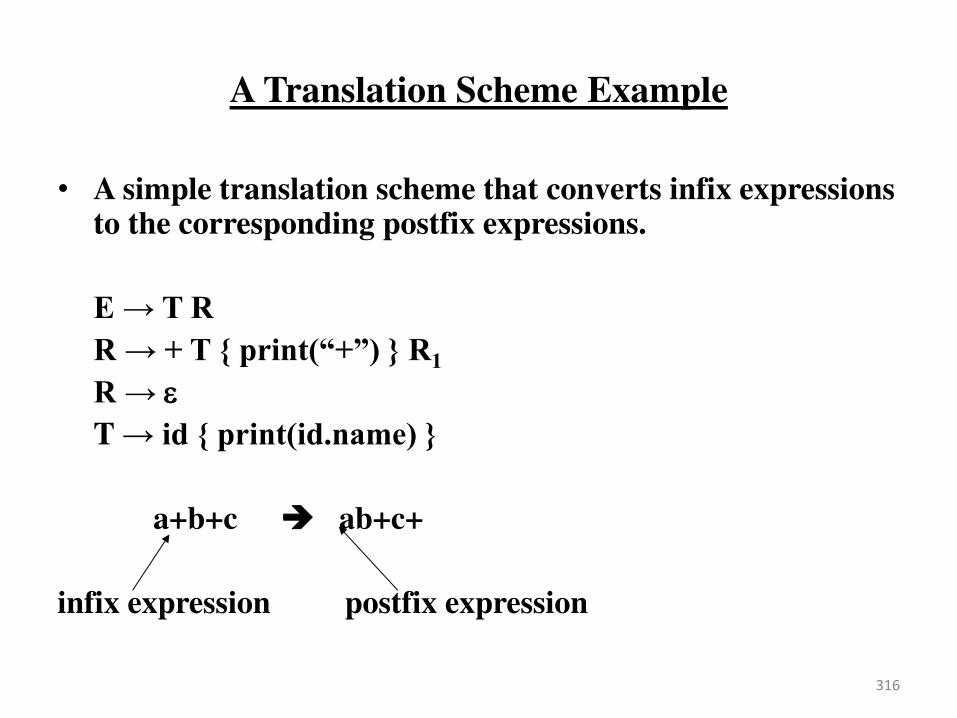
A Translation Scheme Example

• A simple translation scheme that converts infix expressions to the corresponding postfix expressions.

E T R

R + T { print(“+”) } R1

R T id { print(id.name) }

a+b+c ab+c+

infix expression postfix expression

316

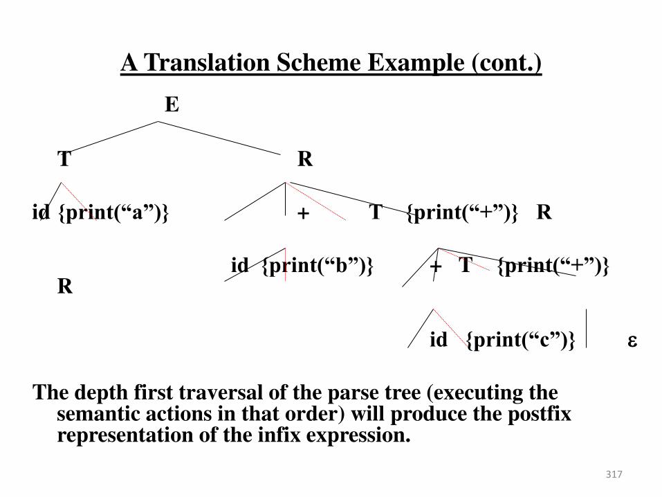
A Translation Scheme Example (cont.)

E

T R

id {print(“a”)} + T {print(“+”)} R

id {print(“b”)} + T {print(“+”)} R

id {print(“c”)}

The depth first traversal of the parse tree (executing the semantic actions in that order) will produce the postfix representation of the infix expression.

317

Inherited Attributes in Translation Schemes

• If a translation scheme has to contain both synthesized and inherited attributes, we have to observe the following rules:

1. An inherited attribute of a symbol on the right side of a production must be computed in a semantic action before that symbol.

2. A semantic action must not refer to a synthesized attribute of a symbol to the right of that semantic action.

3. A synthesized attribute for the non-terminal on the left can only be computed after all attributes it references have been computed (we normally put this semantic action at the end of the right side of the production).

• With a L-attributed syntax-directed definition, it is always possible to construct a corresponding translation scheme which satisfies these three conditions (This may not be possible for a general syntax-directed translation).

318

Top-Down Translation

• We will look at the implementation of L-attributed

definitions during predictive parsing.

• Instead of the syntax-directed translations, we will work

with translation schemes.

• We will see how to evaluate inherited attributes (in L-

attributed definitions) during recursive predictive parsing.

• We will also look at what happens to attributes during the

left-recursion elimination in the left-recursive grammars.

319

A Translation Scheme with Inherited Attributes

D T id { addtype(id.entry,T.type), L.in = T.type } L

T int { T.type = integer }

T real { T.type = real }

L id { addtype(id.entry,L.in), L1.in = L.in } L1

L

• This is a translation scheme for an L-attributed definitions.

320

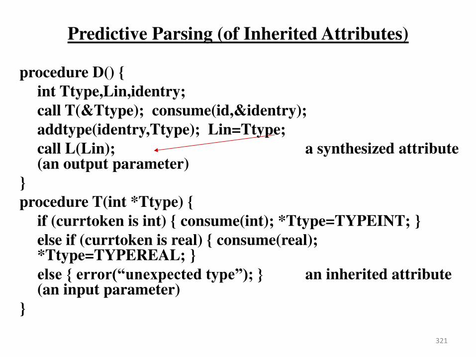
Predictive Parsing (of Inherited Attributes)

procedure D() {

int Ttype,Lin,identry;

call T(&Ttype); consume(id,&identry);

addtype(identry,Ttype); Lin=Ttype;

call L(Lin); a synthesized attribute (an output parameter)

}

procedure T(int *Ttype) {

if (currtoken is int) { consume(int); *Ttype=TYPEINT; }

else if (currtoken is real) { consume(real); *Ttype=TYPEREAL; }

else { error(“unexpected type”); } an inherited attribute (an input parameter)

}

321

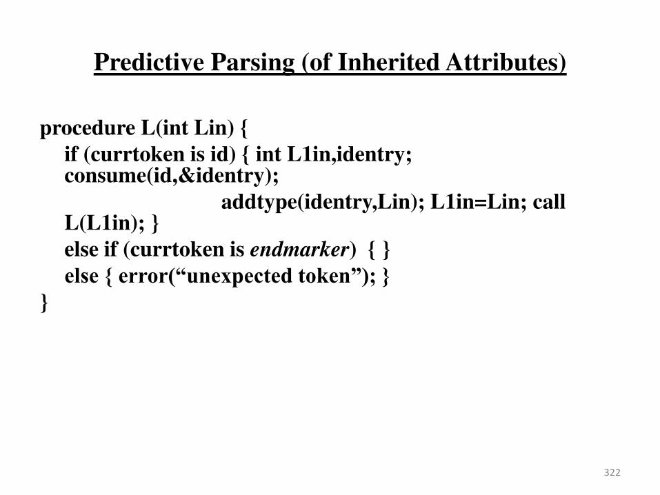
Predictive Parsing (of Inherited Attributes)

procedure L(int Lin) {

if (currtoken is id) { int L1in,identry; consume(id,&identry);

addtype(identry,Lin); L1in=Lin; call L(L1in); }

else if (currtoken is endmarker) { }

else { error(“unexpected token”); }

}

322

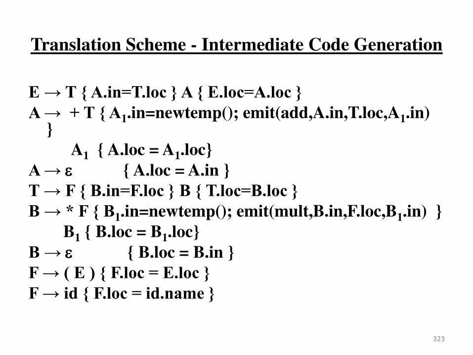
Translation Scheme - Intermediate Code Generation

E T { A.in=T.loc } A { E.loc=A.loc }

A + T { A1.in=newtemp(); emit(add,A.in,T.loc,A1.in) }

A1 { A.loc = A1.loc}

A { A.loc = A.in } T F { B.in=F.loc } B { T.loc=B.loc }

B * F { B1.in=newtemp(); emit(mult,B.in,F.loc,B1.in) }

B1 { B.loc = B1.loc}

B { B.loc = B.in } F ( E ) { F.loc = E.loc }

F id { F.loc = id.name }

323

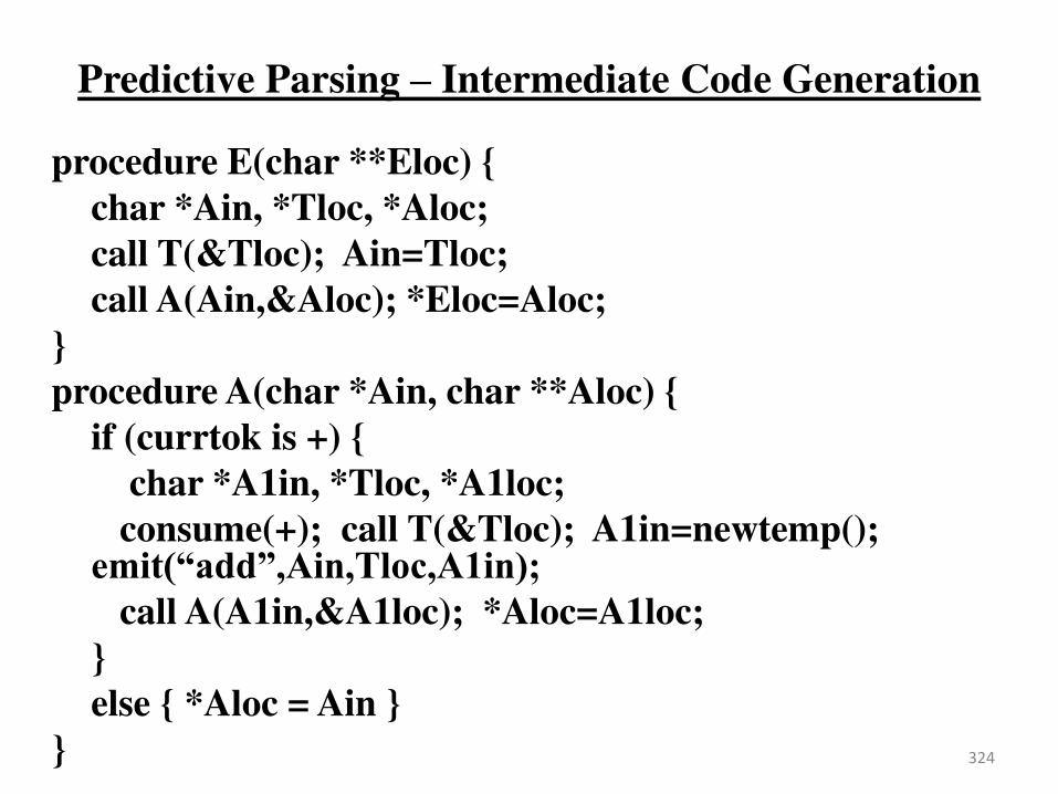
Predictive Parsing – Intermediate Code Generation

procedure E(char **Eloc) {

char *Ain, *Tloc, *Aloc;

call T(&Tloc); Ain=Tloc;

call A(Ain,&Aloc); *Eloc=Aloc;

}

procedure A(char *Ain, char **Aloc) {

if (currtok is +) {

char *A1in, *Tloc, *A1loc;

consume(+); call T(&Tloc); A1in=newtemp(); emit(“add”,Ain,Tloc,A1in);

call A(A1in,&A1loc); *Aloc=A1loc;

}

else { *Aloc = Ain }

}

324

Predictive Parsing (cont.)

procedure T(char **Tloc) {

char *Bin, *Floc, *Bloc;

call F(&Floc); Bin=Floc;

call B(Bin,&Bloc); *Tloc=Bloc;

}

procedure B(char *Bin, char **Bloc) {

if (currtok is *) {

char *B1in, *Floc, *B1loc;

consume(+); call F(&Floc); B1in=newtemp(); e it ult ,Bi ,Flo ,B i ;

call B(B1in,&B1loc); Bloc=B1loc;

}

325

Predictive Parsing (cont.)

else { *Bloc = Bin }

}

procedure F(char **Floc) {

if u tok is { ha *Elo ; o su e ; all E &Elo ; o su e ; *Flo =Elo }

else { char *idname; consume(id,&idname);

*Floc=idname }

}

326

Bottom-Up Evaluation of Inherited Attributes

• Using a top-down translation scheme, we can implement any L-attributed definition based on a LL(1) grammar.

• Using a bottom-up translation scheme, we can also implement any L-attributed definition based on a LL(1) grammar (each LL(1) grammar is also an LR(1) grammar).

• In addition to the L-attributed definitions based on LL(1) grammars, we can implement some of L-attributed definitions based on LR(1) grammars (not all of them) using the bottom-up translation scheme.

327

Removing Embedding Semantic Actions

• In bottom-up evaluation scheme, the semantic actions are evaluated during the reductions.

• During the bottom-up evaluation of S-attributed definitions, we have a parallel stack to hold synthesized attributes.

• Problem: where are we going to hold inherited attributes?

• A Solution:

328

Removing Embedding Semantic Actions

– We will convert our grammar to an equivalent grammar to guarantee to the followings.

– All embedding semantic actions in our translation scheme will be moved into the end of the production rules.

– All inherited attributes will be copied into the synthesized attributes (most of the time synthesized attributes of new non-terminals).

– Thus we will be evaluate all semantic actions during reductions, and we find a place to store an inherited attribute.

329

Removing Embedding Semantic Actions

• To transform our translation scheme into an equivalent

translation scheme:

1. Remove an embedding semantic action Si, put new a non-

terminal Mi instead of that semantic action.

2. Put that semantic action Si into the end of a new

production rule Mi for that non-terminal Mi.

3. That semantic action Si will be evaluated when this new

production rule is reduced.

4. The evaluation order of the semantic rules are not

changed by this transformation.

330

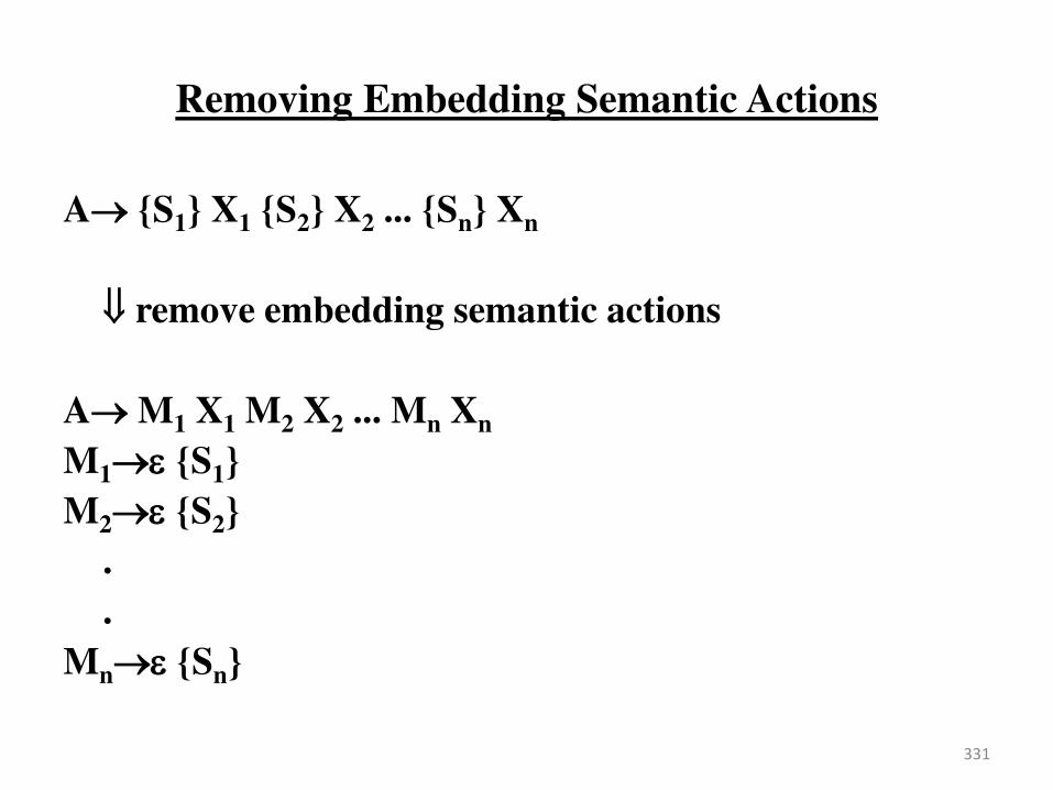
Removing Embedding Semantic Actions

A {S1} X1 {S2} X2 ... {Sn} Xn

remove embedding semantic actions

A M1 X1 M2 X2 ... Mn Xn

M1 {S1}

M2 {S2}

.

.

Mn {Sn}

331

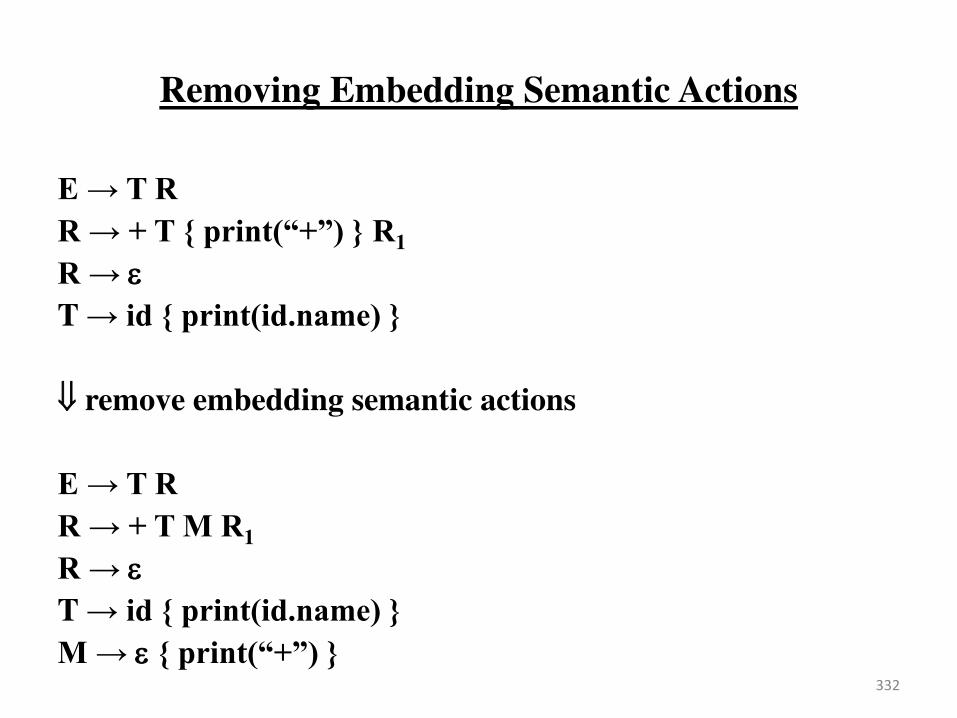
Removing Embedding Semantic Actions

E T R

R + T { print(“+”) } R1

R T id { print(id.name) }

remove embedding semantic actions

E T R

R + T M R1

R T id { print(id.name) }

M { print(“+”) } 332

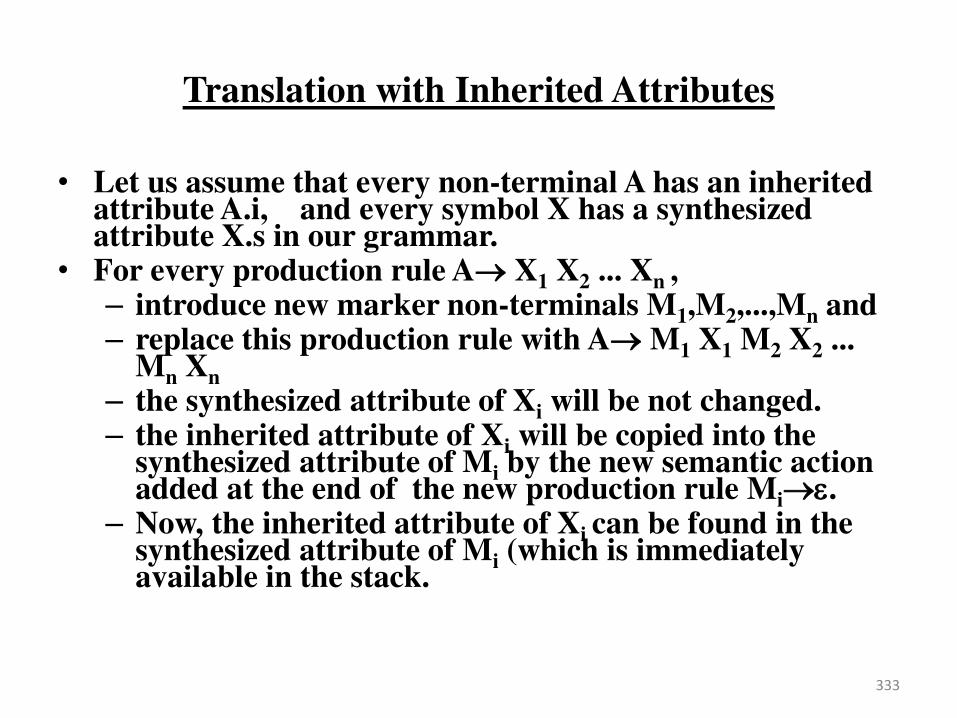
Translation with Inherited Attributes

• Let us assume that every non-terminal A has an inherited attribute A.i, and every symbol X has a synthesized attribute X.s in our grammar.

• For every production rule A X1 X2 ... Xn , – introduce new marker non-terminals M1,M2,...,Mn and – replace this production rule with A M1 X1 M2 X2 ...

Mn Xn

– the synthesized attribute of Xi will be not changed. – the inherited attribute of Xi will be copied into the

synthesized attribute of Mi by the new semantic action added at the end of the new production rule Mi.

– Now, the inherited attribute of Xi can be found in the synthesized attribute of Mi (which is immediately available in the stack.

333

Translation with Inherited Attributes

S {A.i=1} A {S.s=k(A.i,A.s)}

A {B.i=f(A.i)} B {C.i=g(A.i,B.i,B.s)} C {A.s= h(A.i,B.i,B.s,C.i,C.s)}

B b {B.s=m(B.i,b.s)}

C c {C.s=n(C.i,c.s)}

S {M1.i=1} M1 {A.i=M1.s} A {S.s=k(M1.s,A.s)}

A {M2.i=f(A.i)} M2 {B.i=M2.s} B {M3.i=g(A.i,M2.s,B.s)} M3 {C.i=M3.s} C {A.s= h(A.i,

M2.s,B.s, M3.s,C.s)}

B b {B.s=m(B.i,b.s)}

C c {C.s=n(C.i,c.s)}

M1 {M1.s=M1.i}

M2 {M2.s=M2.i}

M3 {M3.s=M3.i}

334

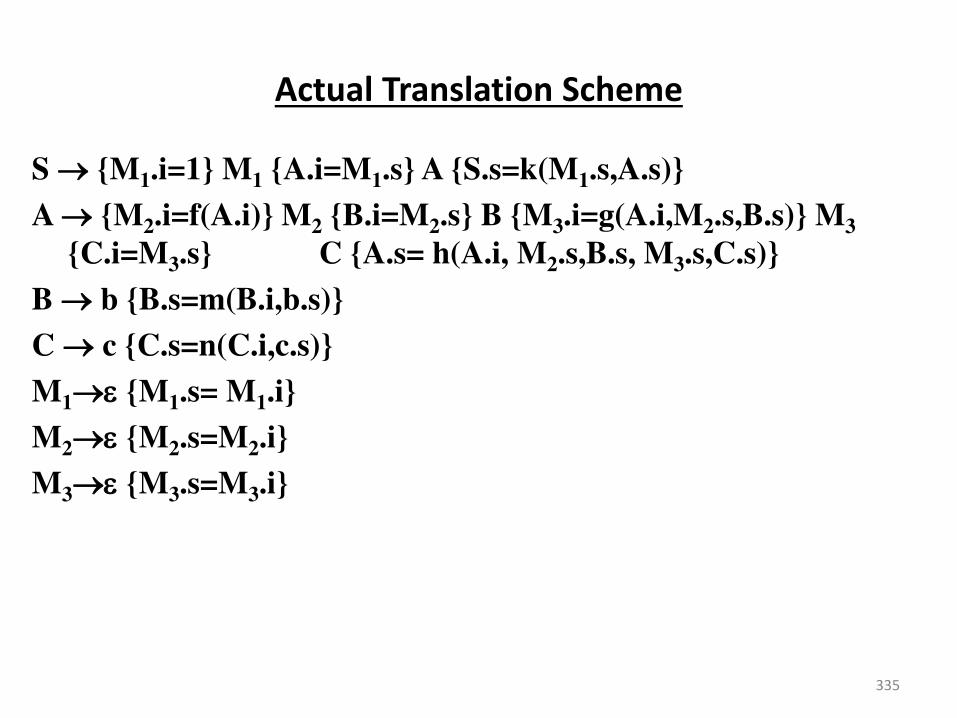
Actual Translation Scheme

S {M1.i=1} M1 {A.i=M1.s} A {S.s=k(M1.s,A.s)}

A {M2.i=f(A.i)} M2 {B.i=M2.s} B {M3.i=g(A.i,M2.s,B.s)} M3 {C.i=M3.s} C {A.s= h(A.i, M2.s,B.s, M3.s,C.s)}

B b {B.s=m(B.i,b.s)}

C c {C.s=n(C.i,c.s)}

M1 {M1.s= M1.i}

M2 {M2.s=M2.i}

M3 {M3.s=M3.i}

335

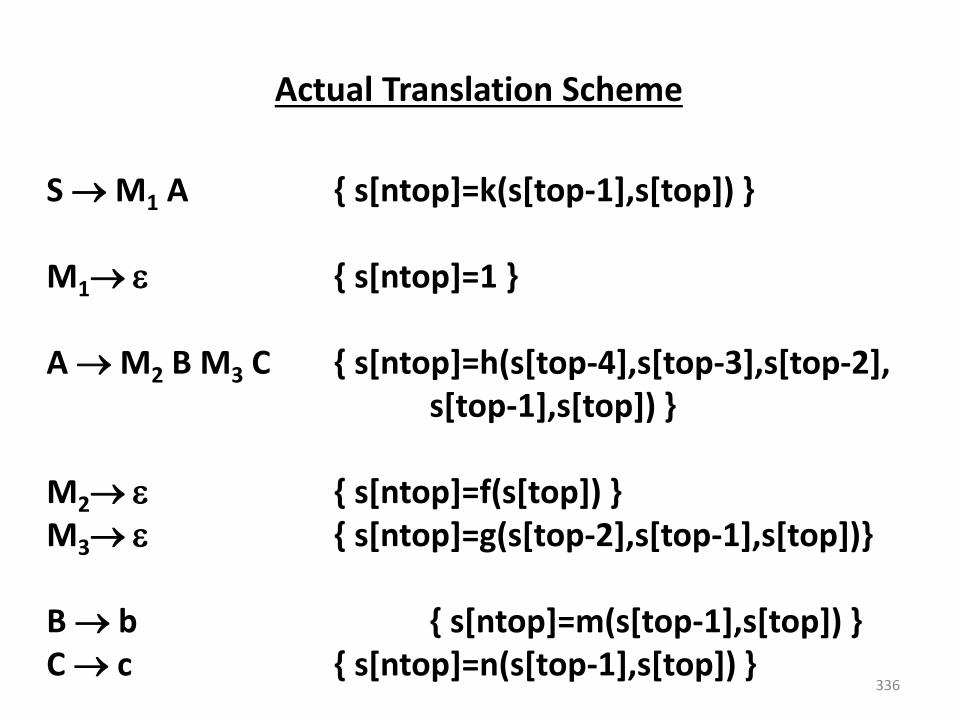
Actual Translation Scheme

S M1 A { s[ntop]=k(s[top-1],s[top]) }

M1 { s[ntop]=1 }

A M2 B M3 C { s[ntop]=h(s[top-4],s[top-3],s[top-2],

s[top-1],s[top]) }

M2 { s[ntop]=f(s[top]) }

M3 { s[ntop]=g(s[top-2],s[top-1],s[top])}

B b { s[ntop]=m(s[top-1],s[top]) }

C c { s[ntop]=n(s[top-1],s[top]) }

336

Evaluation of Attributes

S

S.s=k(1,h(..))

A.i=1

A

A.s=h(1,f(1),m(..),g(..),n(..))

B.i=f(1) C.i=g(1,f(1),m(..))

B C

B.s=m(f(1),b.s) C.s=n(g(..),c.s)

b c

337

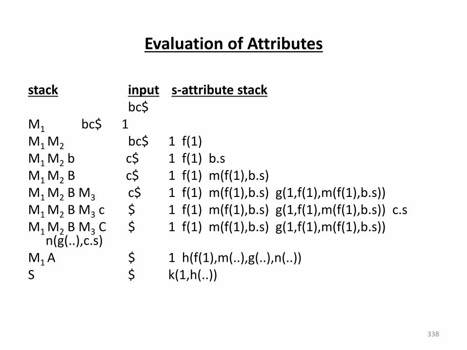
Evaluation of Attributes

stack input s-attribute stack

bc$

M1 bc$ 1

M1 M2 bc$ 1 f(1)

M1 M2 b c$ 1 f(1) b.s

M1 M2 B c$ 1 f(1) m(f(1),b.s)

M1 M2 B M3 c$ 1 f(1) m(f(1),b.s) g(1,f(1),m(f(1),b.s))

M1 M2 B M3 c $ 1 f(1) m(f(1),b.s) g(1,f(1),m(f(1),b.s)) c.s

M1 M2 B M3 C $ 1 f(1) m(f(1),b.s) g(1,f(1),m(f(1),b.s)) n(g(..),c.s)

M1 A $ 1 h(f(1),m(..),g(..),n(..))

S $ k(1,h(..))

338

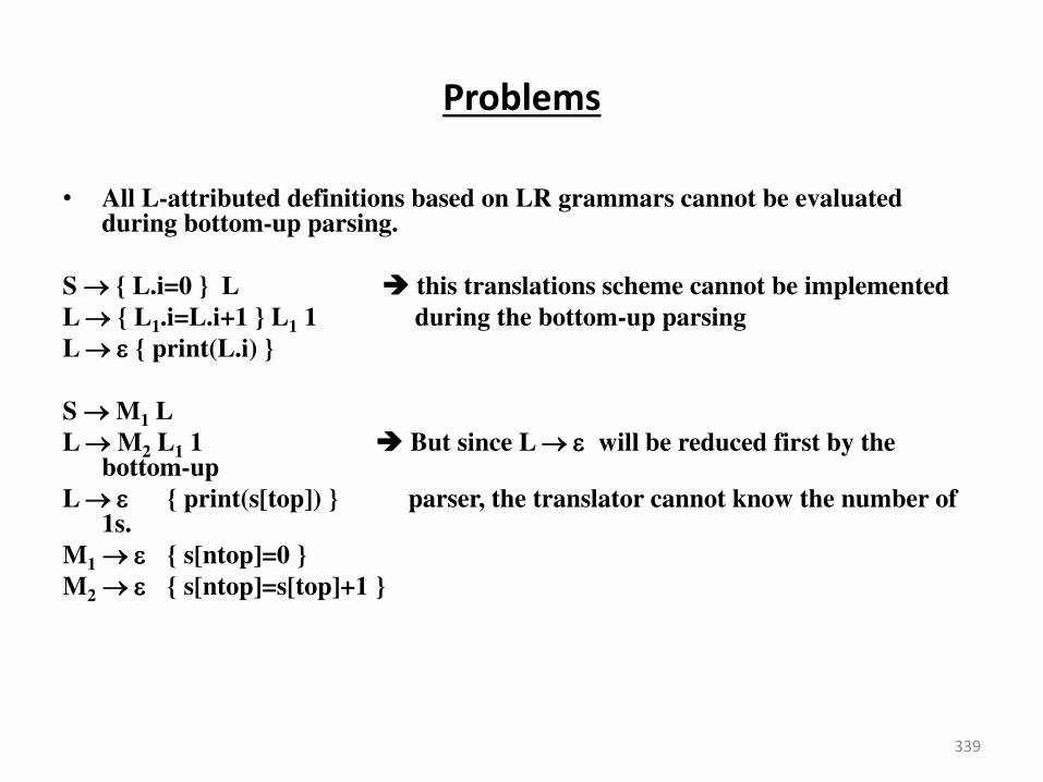
Problems

• All L-attributed definitions based on LR grammars cannot be evaluated during bottom-up parsing.

S { L.i=0 } L this translations scheme cannot be implemented

L { L1.i=L.i+1 } L1 1 during the bottom-up parsing

L { print(L.i) }

S M1 L

L M2 L1 1 But since L will be reduced first by the bottom-up

L { print(s[top]) } parser, the translator cannot know the number of 1s.

M1 { s[ntop]=0 }

M2 { s[ntop]=s[top]+1 }

339

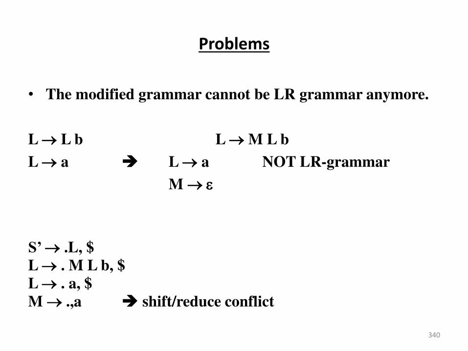
Problems

• The modified grammar cannot be LR grammar anymore.

L L b L M L b

L a L a NOT LR-grammar

M

S’ .L, $ L . M L b, $ L . a, $ M .,a shift/reduce conflict

340

Intermediate Code Generation

• Intermediate codes are machine independent codes, but they are close to machine instructions.

• The given program in a source language is converted to an equivalent program in an intermediate language by the intermediate code generator.

• Intermediate language can be many different languages, and the designer of the compiler decides this intermediate language.

– syntax trees can be used as an intermediate language.

341

Intermediate Code Generation

– postfix notation can be used as an intermediate language.

– three-address code (Quadraples) can be used as an intermediate language

• we will use quadraples to discuss intermediate code generation

• quadraples are close to machine instructions, but they are not actual machine instructions.

– some programming languages have well defined intermediate languages.

• java – java virtual machine

• prolog – warren abstract machine

• In fact, there are byte-code emulators to execute instructions in these intermediate languages.

342

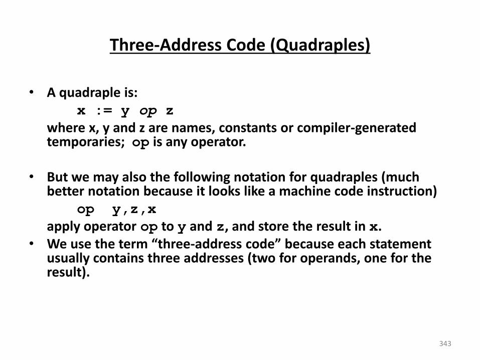
Three-Address Code (Quadraples)

• A quadraple is:

x := y op z where x, y and z are names, constants or compiler-generated

temporaries; op is any operator.

• But we may also the following notation for quadraples (much better notation because it looks like a machine code instruction)

op y,z,x apply operator op to y and z, and store the result in x.

• We use the te th ee-add ess ode e ause ea h state e t usually contains three addresses (two for operands, one for the result).

343

Three-Address Statements

Binary Operator: op y,z,result or result := y op z where op is a binary arithmetic or logical operator. This binary

operator is applied to y and z, and the result of the operation is stored in result.

Ex: add a,b,c gt a,b,c addr a,b,c addi a,b,c Unary Operator: op y,,result or result := op y where op is a unary arithmetic or logical operator. This unary

operator is applied to y, and the result of the operation is stored in result.

Ex: uminus a,,c not a,,c int to real a,,c

344

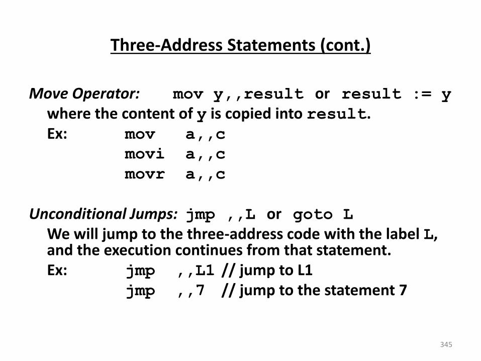
Three-Address Statements (cont.)

Move Operator: mov y,,result or result := y where the content of y is copied into result.

Ex: mov a,,c movi a,,c movr a,,c Unconditional Jumps: jmp ,,L or goto L We will jump to the three-address code with the label L,

and the execution continues from that statement.

Ex: jmp ,,L1 // jump to L1

jmp ,,7 // jump to the statement 7

345

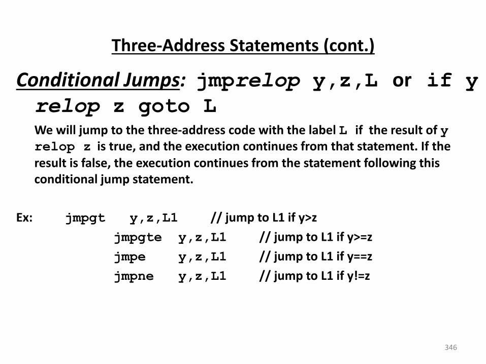
Three-Address Statements (cont.)

Conditional Jumps: jmprelop y,z,L or if y relop z goto L

We will jump to the three-address code with the label L if the result of y relop z is true, and the execution continues from that statement. If the

result is false, the execution continues from the statement following this

conditional jump statement.

Ex: jmpgt y,z,L1 // jump to L1 if y>z

jmpgte y,z,L1 // jump to L1 if y>=z

jmpe y,z,L1 // jump to L1 if y==z

jmpne y,z,L1 // jump to L1 if y!=z

346

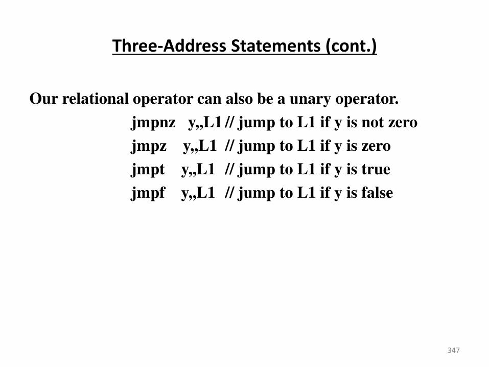
Three-Address Statements (cont.)

Our relational operator can also be a unary operator.

jmpnz y,,L1 // jump to L1 if y is not zero

jmpz y,,L1 // jump to L1 if y is zero

jmpt y,,L1 // jump to L1 if y is true

jmpf y,,L1 // jump to L1 if y is false

347

Three-Address Statements (cont.)

Procedure Parameters: param x,, or param x

Procedure Calls: call p,n, or call p,n

where x is an actual parameter, we invoke the procedure p

with n parameters.

Ex: param x1,,

param x2,,

p(x1,...,xn)

param xn,,

call p,n,

f(x+1,y) add x,1,t1

param t1,,

param y,,

call f,2, 348

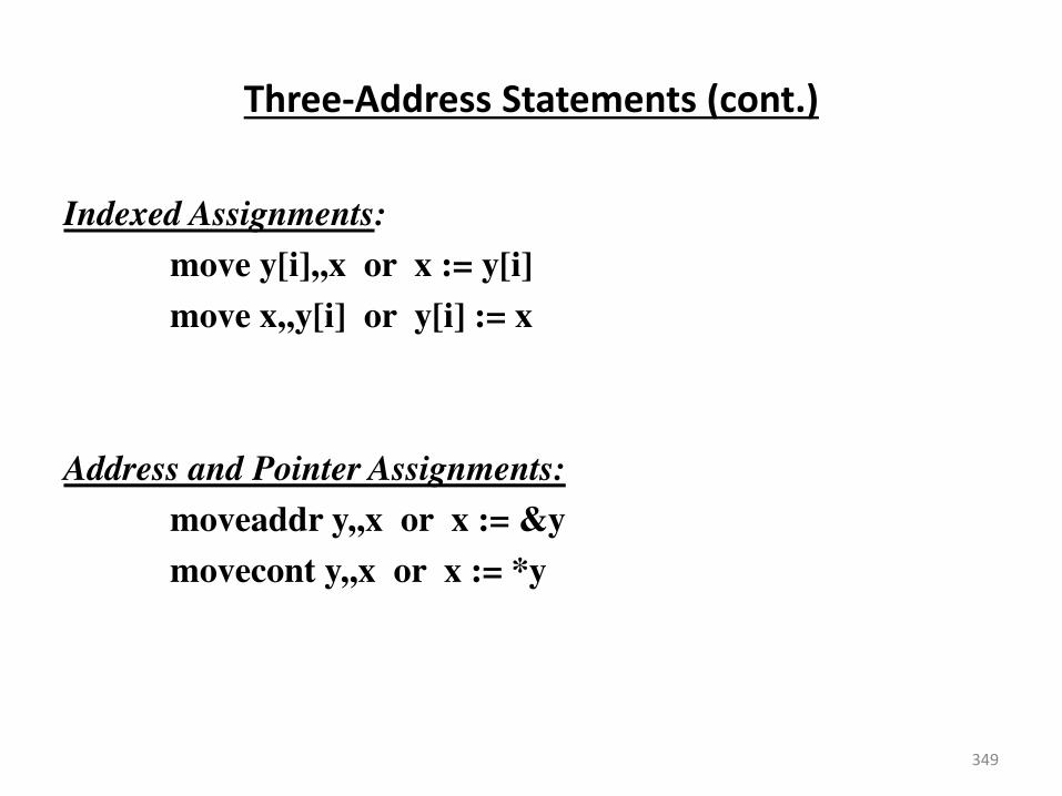
Three-Address Statements (cont.)

Indexed Assignments:

move y[i],,x or x := y[i]

move x,,y[i] or y[i] := x

Address and Pointer Assignments:

moveaddr y,,x or x := &y

movecont y,,x or x := *y

349

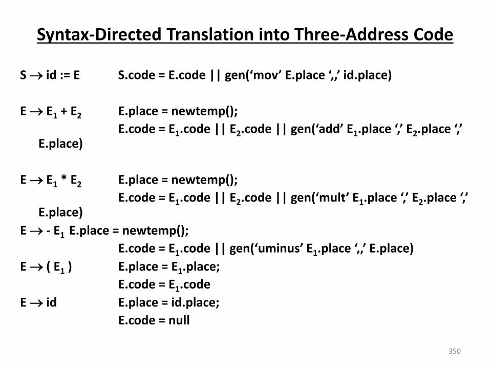
Syntax-Directed Translation into Three-Address Code

S id := E “. ode = E. ode || ge o E.pla e ,, id.pla e

E E1 + E2 E.place = newtemp();

E.code = E1.code || E2. ode || ge add E1.pla e , E2.pla e , E.place)

E E1 * E2 E.place = newtemp();

E.code = E1.code || E2. ode || ge ult E1.pla e , E2.pla e , E.place)

E - E1 E.place = newtemp();

E.code = E1. ode || ge u i us E1.pla e ,, E.pla e

E ( E1 ) E.place = E1.place;

E.code = E1.code

E id E.place = id.place;

E.code = null

350

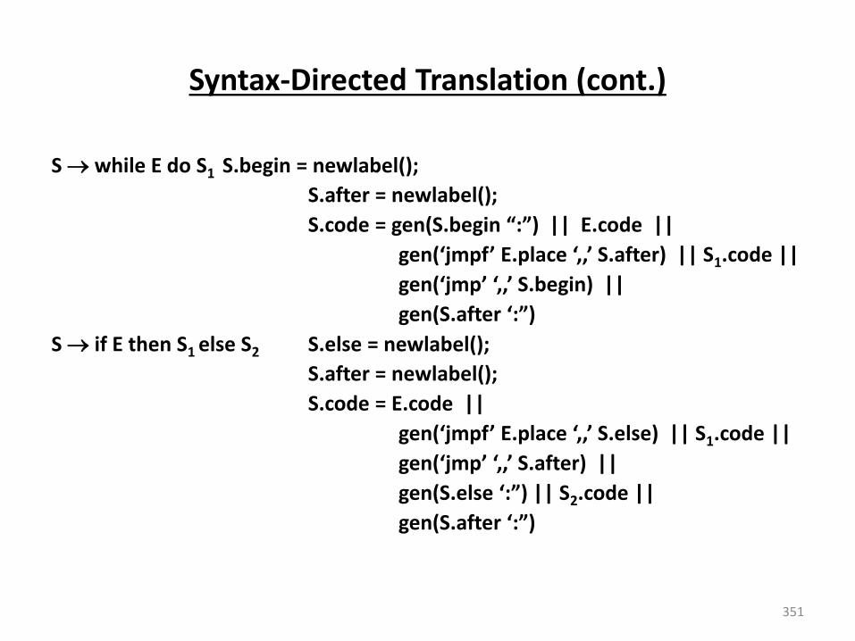
Syntax-Directed Translation (cont.)

S while E do S1 S.begin = newlabel();

S.after = newlabel();

“. ode = ge “. egi : || E. ode ||

ge j pf E.pla e ,, “.afte || “1.code ||

ge j p ,, “. egi || ge “.afte :

S if E then S1 else S2 S.else = newlabel();

S.after = newlabel();

S.code = E.code ||

ge j pf E.pla e ,, “.else || “1.code ||

ge j p ,, “.afte ||

ge “.else : || “2.code ||

ge “.afte :

351

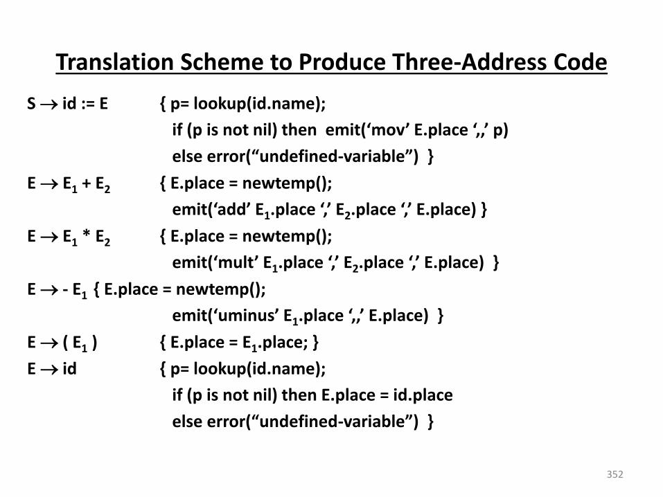
Translation Scheme to Produce Three-Address Code

S id := E { p= lookup(id.name);

if p is ot il the e it o E.pla e ,, p

else e o u defi ed- a ia le }

E E1 + E2 { E.place = newtemp();

e it add E1.pla e , E2.pla e , E.pla e }

E E1 * E2 { E.place = newtemp();

e it ult E1.pla e , E2.pla e , E.pla e }

E - E1 { E.place = newtemp();

e it u i us E1.pla e ,, E.pla e }

E ( E1 ) { E.place = E1.place; }

E id { p= lookup(id.name);

if (p is not nil) then E.place = id.place

else e o u defi ed- a ia le }

352

Translation Scheme with Locations

S id := { E.inloc = S.inloc } E { p = lookup(id.name); if p is ot il the { e it E.outlo o E.pla e ,, p ;

S.outloc=E.outloc+1 } else { e o u defi ed- a ia le ; “.outlo =E.outlo

} } E { E1.inloc = E.inloc } E1 + { E2.inloc = E1.outloc } E2 { E.place = newtemp(); emit(E2.outlo add E1.pla e ,

E2.pla e , E.place); E.outloc=E2.outloc+1 } E { E1.inloc = E.inloc } E1 + { E2.inloc = E1.outloc } E2 { E.place = newtemp(); emit(E2.outlo ult E1.pla e ,

E2.pla e , E.place); E.outloc=E2.outloc+1 }

353

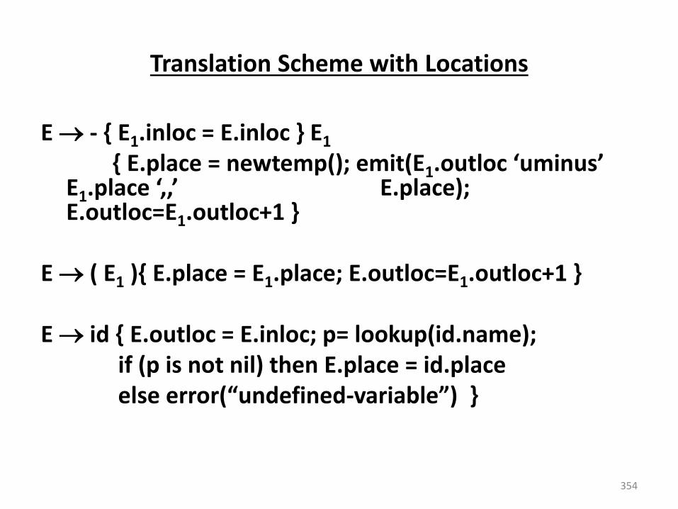
Translation Scheme with Locations

E - { E1.inloc = E.inloc } E1

{ E.place = newtemp(); emit(E1.outlo u i us E1.pla e ,, E.place); E.outloc=E1.outloc+1 }

E ( E1 ){ E.place = E1.place; E.outloc=E1.outloc+1 }

E id { E.outloc = E.inloc; p= lookup(id.name);

if (p is not nil) then E.place = id.place

else e o u defi ed- a ia le }

354

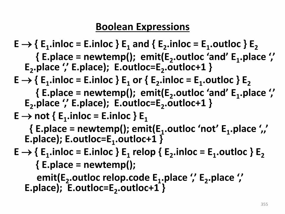
Boolean Expressions

E { E1.inloc = E.inloc } E1 and { E2.inloc = E1.outloc } E2

{ E.place = newtemp(); emit(E2.outlo a d E1.pla e , E2.pla e , E.pla e ; E.outlo =E2.outloc+1 }

E { E1.inloc = E.inloc } E1 or { E2.inloc = E1.outloc } E2

{ E.place = newtemp(); emit(E2.outlo a d E1.pla e , E2.pla e , E.pla e ; E.outlo =E2.outloc+1 }

E not { E1.inloc = E.inloc } E1

{ E.place = newtemp(); emit(E1.outlo ot E1.pla e ,, E.place); E.outloc=E1.outloc+1 }

E { E1.inloc = E.inloc } E1 relop { E2.inloc = E1.outloc } E2

{ E.place = newtemp();

emit(E2.outloc relop.code E1.pla e , E2.pla e , E.place); E.outloc=E2.outloc+1 }

355

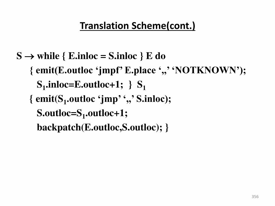
Translation Scheme(cont.)

S while { E.inloc = S.inloc } E do

{ emit(E.outloc ‘jmpf’ E.place ‘,,’ ‘NOTKNO→N’); S1.inloc=E.outloc+1; } S1

{ emit(S1.outloc ‘jmp’ ‘,,’ S.inloc); S.outloc=S1.outloc+1;

backpatch(E.outloc,S.outloc); }

356

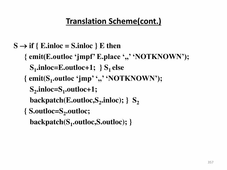
Translation Scheme(cont.)

S if { E.inloc = S.inloc } E then

{ emit(E.outloc ‘jmpf’ E.place ‘,,’ ‘NOTKNO→N’); S1.inloc=E.outloc+1; } S1 else

{ emit(S1.outloc ‘jmp’ ‘,,’ ‘NOTKNO→N’); S2.inloc=S1.outloc+1;

backpatch(E.outloc,S2.inloc); } S2

{ S.outloc=S2.outloc;

backpatch(S1.outloc,S.outloc); }

357

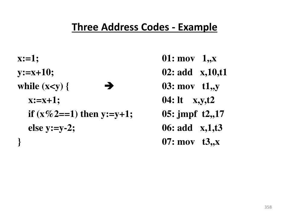
Three Address Codes - Example

x:=1; 01: mov 1,,x

y:=x+10; 02: add x,10,t1

while (x<y) { 03: mov t1,,y

x:=x+1; 04: lt x,y,t2

if (x%2==1) then y:=y+1; 05: jmpf t2,,17

else y:=y-2; 06: add x,1,t3

} 07: mov t3,,x

358

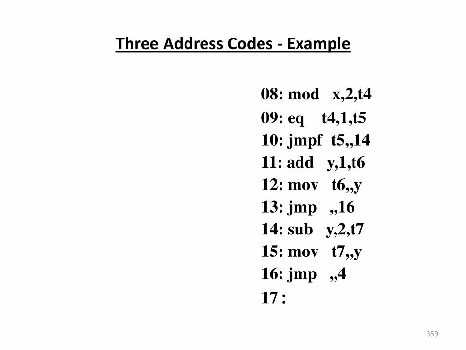
Three Address Codes - Example

08: mod x,2,t4

09: eq t4,1,t5

10: jmpf t5,,14

11: add y,1,t6

12: mov t6,,y

13: jmp ,,16

14: sub y,2,t7

15: mov t7,,y

16: jmp ,,4

17:

359

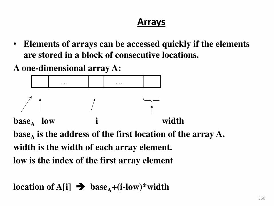
Arrays

• Elements of arrays can be accessed quickly if the elements

are stored in a block of consecutive locations.

A one-dimensional array A:

baseA low i width

baseA is the address of the first location of the array A,

width is the width of each array element.

low is the index of the first array element

location of A[i] baseA+(i-low)*width

… …

360

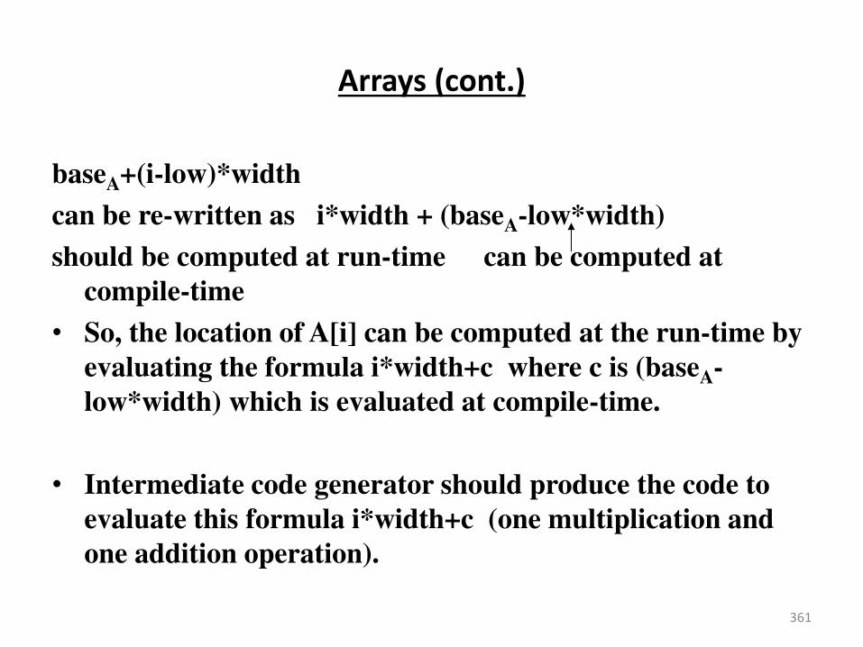
Arrays (cont.)

baseA+(i-low)*width

can be re-written as i*width + (baseA-low*width)

should be computed at run-time can be computed at

compile-time

• So, the location of A[i] can be computed at the run-time by

evaluating the formula i*width+c where c is (baseA-

low*width) which is evaluated at compile-time.

• Intermediate code generator should produce the code to

evaluate this formula i*width+c (one multiplication and

one addition operation).

361

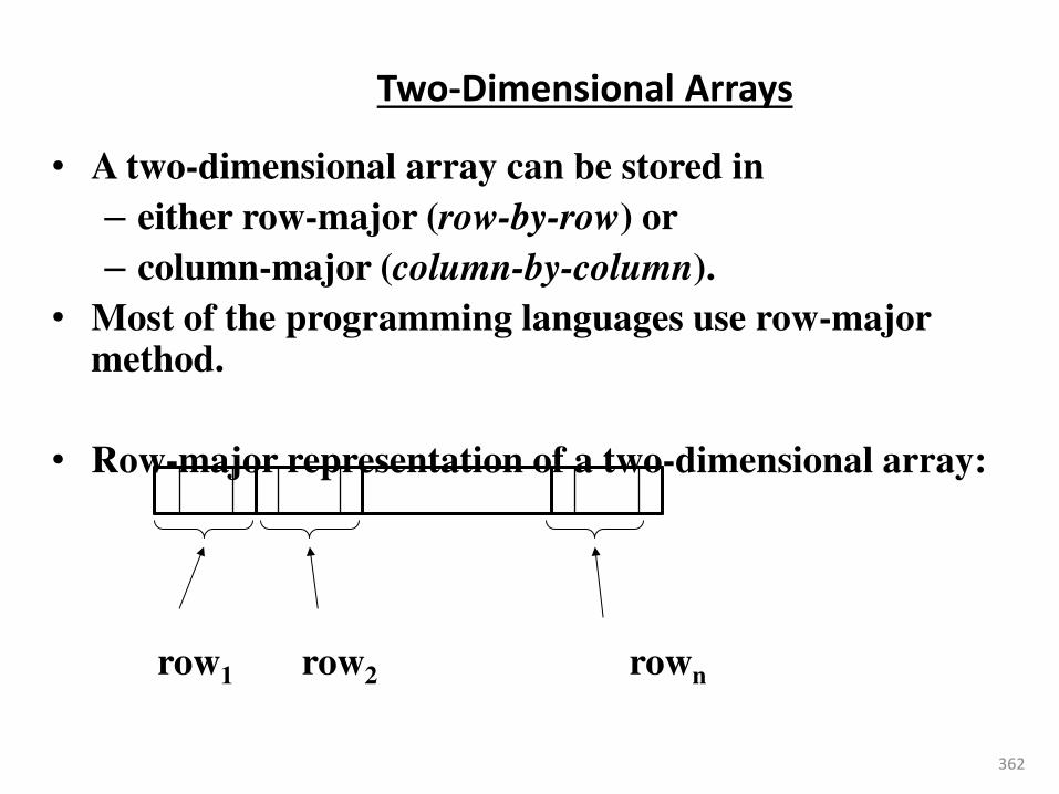
Two-Dimensional Arrays

• A two-dimensional array can be stored in

– either row-major (row-by-row) or

– column-major (column-by-column).

• Most of the programming languages use row-major method.

• Row-major representation of a two-dimensional array:

row1 row2 rown

362

Two-Dimensional Arrays (cont.)

• The location of A[i1,i2] is

baseA+ ((i1-low1)*n2+i2-low2)*width

baseA is the location of the array A.

low1 is the index of the first row

low2 is the index of the first column

n2 is the number of elements in each row

width is the width of each array element

• Again, this formula can be re-written as

((i1*n2)+i2)*width + (baseA-((low1*n1)+low2)*width)

should be computed at run-time can be computed at compile-time

363

Multi-Dimensional Arrays

• In general, the location of A[i1,i2,...,ik] is

(( ... ((i1*n2)+i2) ...)*nk+ik)*width + (baseA-

((...((low1*n1)+low2)...)*nk+lowk)*width)

• So, the intermediate code generator should produce the codes

to evaluate the following formula (to find the location of

A[i1,i2,...,ik]) :

(( ... ((i1*n2)+i2) ...)*nk+ik)*width + c

• To evaluate the (( ... ((i1*n2)+i2) ...)*nk+ik portion of this

formula, we can use the recurrence equation:

e1 = i1

em = em-1 * nm + im

364

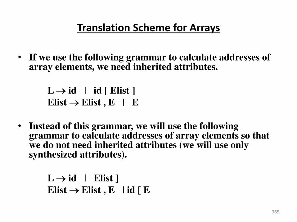
Translation Scheme for Arrays

• If we use the following grammar to calculate addresses of array elements, we need inherited attributes.

L id | id [ Elist ]

Elist Elist , E | E

• Instead of this grammar, we will use the following grammar to calculate addresses of array elements so that we do not need inherited attributes (we will use only synthesized attributes).

L id | Elist ]

Elist Elist , E | id [ E

365

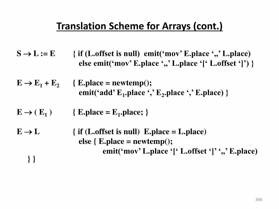
Translation Scheme for Arrays (cont.)

S L := E { if (L.offset is null) emit(‘mov’ E.place ‘,,’ L.place) else emit(‘mov’ E.place ‘,,’ L.place ‘[‘ L.offset ‘]’) }

E E1 + E2 { E.place = newtemp(); emit(‘add’ E1.place ‘,’ E2.place ‘,’ E.place) }

E ( E1 ) { E.place = E1.place; }

E L { if (L.offset is null) E.place = L.place)

else { E.place = newtemp();

emit(‘mov’ L.place ‘[‘ L.offset ‘]’ ‘,,’ E.place) } }

366

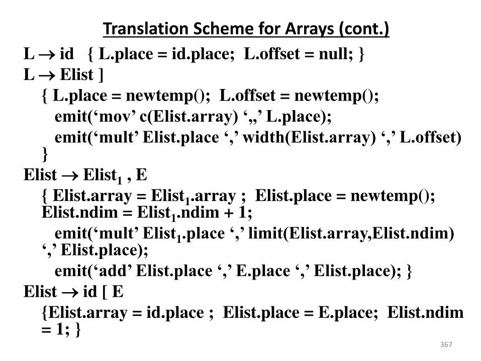
Translation Scheme for Arrays (cont.)

L id { L.place = id.place; L.offset = null; }

L Elist ] { L.place = newtemp(); L.offset = newtemp();

emit(‘mov’ c(Elist.array) ‘,,’ L.place); emit(‘mult’ Elist.place ‘,’ width(Elist.array) ‘,’ L.offset)

}

Elist Elist1 , E { Elist.array = Elist1.array ; Elist.place = newtemp();

Elist.ndim = Elist1.ndim + 1;

emit(‘mult’ Elist1.place ‘,’ limit(Elist.array,Elist.ndim) ‘,’ Elist.place);

emit(‘add’ Elist.place ‘,’ E.place ‘,’ Elist.place); } Elist id [ E {Elist.array = id.place ; Elist.place = E.place; Elist.ndim

= 1; } 367

Translation Scheme for Arrays – Example1

• A one-dimensional double array A : 5..100

n1=95 width=8 (double) low1=5

• Intermediate codes corresponding to x := A[y]

mov c,,t1 // where c=baseA-(5)*8

mult y,8,t2

mov t1[t2],,t3

mov t3,,x

368

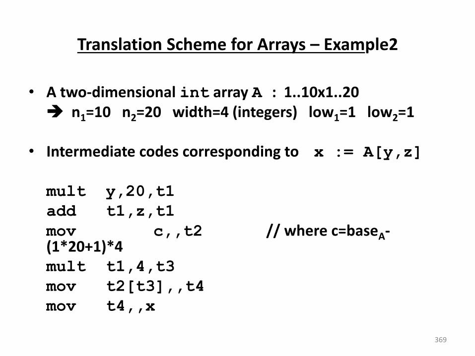
Translation Scheme for Arrays – Example2

• A two-dimensional int array A : 1..10x1..20

n1=10 n2=20 width=4 (integers) low1=1 low2=1

• Intermediate codes corresponding to x := A[y,z]

mult y,20,t1 add t1,z,t1 mov c,,t2 // where c=baseA-

(1*20+1)*4

mult t1,4,t3 mov t2[t3],,t4 mov t4,,x

369

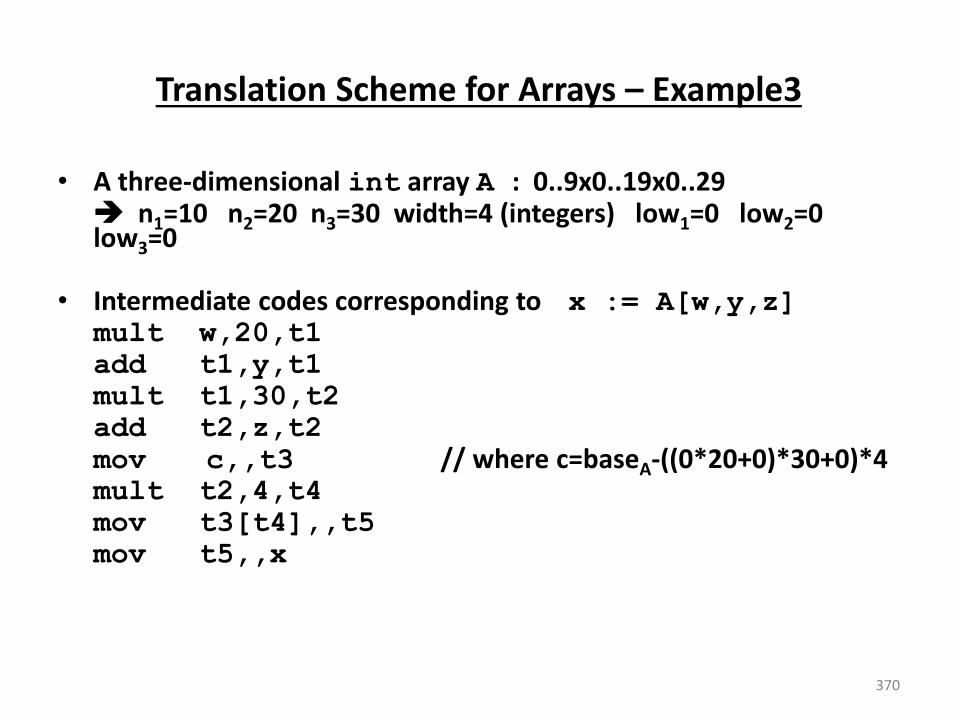
Translation Scheme for Arrays – Example3

• A three-dimensional int array A : 0..9x0..19x0..29 n1=10 n2=20 n3=30 width=4 (integers) low1=0 low2=0

low3=0 • Intermediate codes corresponding to x := A[w,y,z] mult w,20,t1 add t1,y,t1 mult t1,30,t2 add t2,z,t2 mov c,,t3 // where c=baseA-((0*20+0)*30+0)*4 mult t2,4,t4 mov t3[t4],,t5 mov t5,,x

370

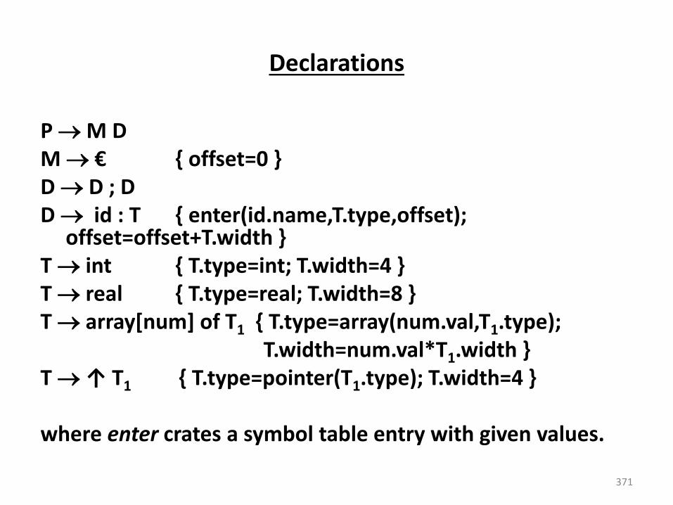
Declarations

P M D

M € { offset=0 }

D D ; D

D id : T { enter(id.name,T.type,offset); offset=offset+T.width }

T int { T.type=int; T.width=4 }

T real { T.type=real; T.width=8 }

T array[num] of T1 { T.type=array(num.val,T1.type);

T.width=num.val*T1.width }

T ↑ T1 { T.type=pointer(T1.type); T.width=4 }

where enter crates a symbol table entry with given values.

371

Nested Procedure Declarations

• For each procedure we should create a symbol table.

mktable(previous) – create a new symbol table where previous is the parent symbol table of this new symbol table

enter(symtable,name,type,offset) – create a new entry for a variable in the given symbol table.

enterproc(symtable,name,newsymbtable) – create a new entry for the procedure in the symbol table of its parent.

372

Nested Procedure Declarations

addwidth(symtable,width) – puts the total width of all entries in the symbol table into the header of that table.

• We will have two stacks:

– tblptr – to hold the pointers to the symbol tables

– offset – to hold the current offsets in the symbol tables in tblptr stack.

373

Nested Procedure Declarations

P M D { addwidth(top(tblptr),top(offset)); pop(tblptr); pop(offset) }

M € { t=mktable(nil); push(t,tblptr); push(0,offset) }

D D ; D

D proc id N D ; S

{ t=top(tblptr); addwidth(t,top(offset));

pop(tblptr); pop(offset);

enterproc(top(tblptr),id.name,t) }

D id : T { enter(top(tblptr),id.name,T.type,top(offset));

top(offset)=top(offset)+T.width }

N € { t=mktable(top(tblptr)); push(t,tblptr); push(0,offset) }

374

Intermediate Code Generation

375

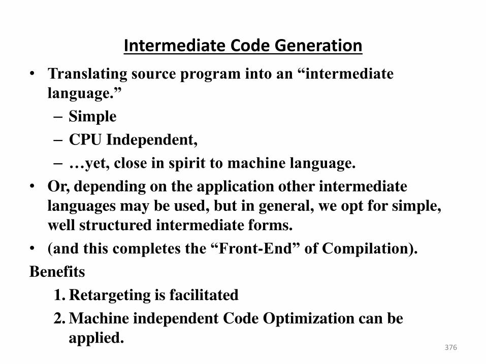
Intermediate Code Generation

• Translating source program into an “intermediate language.”

– Simple

– CPU Independent,

– …yet, close in spirit to machine language. • Or, depending on the application other intermediate

languages may be used, but in general, we opt for simple,

well structured intermediate forms.

• (and this completes the “Front-End” of Compilation). Benefits

1. Retargeting is facilitated

2. Machine independent Code Optimization can be

applied.

376

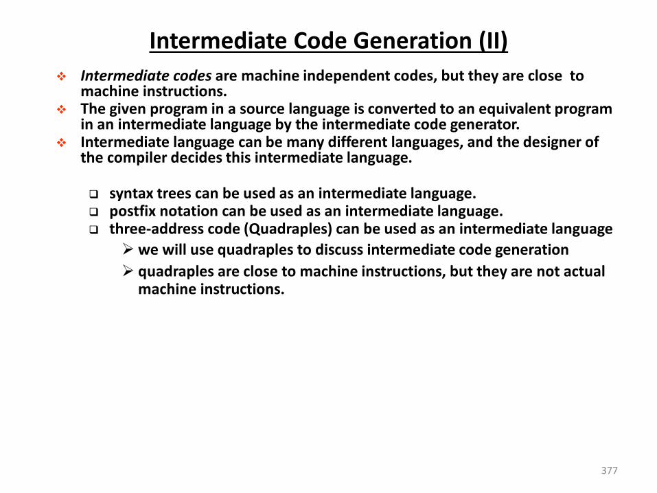
Intermediate Code Generation (II)

377

Intermediate codes are machine independent codes, but they are close to machine instructions.

The given program in a source language is converted to an equivalent program in an intermediate language by the intermediate code generator.

Intermediate language can be many different languages, and the designer of the compiler decides this intermediate language. syntax trees can be used as an intermediate language. postfix notation can be used as an intermediate language. three-address code (Quadraples) can be used as an intermediate language

we will use quadraples to discuss intermediate code generation

quadraples are close to machine instructions, but they are not actual machine instructions.

Types of Intermediate Languages

• Graphical Representations.

– Consider the assignment a:=b*-c+b*-c:

378

assign

a +

* *

uminus uminus b

c c

b

assign

a +

*

uminus

b c

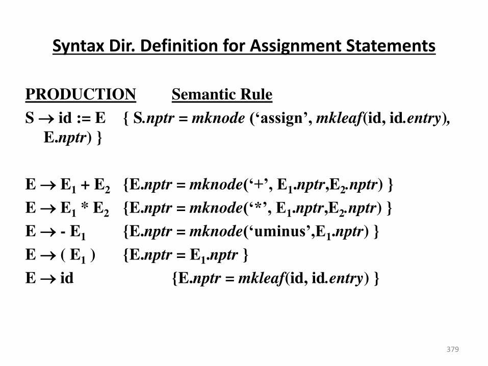
Syntax Dir. Definition for Assignment Statements

PRODUCTION Semantic Rule

S id := E { S.nptr = mknode (‘assign’, mkleaf(id, id.entry), E.nptr) }

E E1 + E2 {E.nptr = mknode(‘+’, E1.nptr,E2.nptr) }

E E1 * E2 {E.nptr = mknode(‘*’, E1.nptr,E2.nptr) }

E - E1 {E.nptr = mknode(‘uminus’,E1.nptr) }

E ( E1 ) {E.nptr = E1.nptr }

E id {E.nptr = mkleaf(id, id.entry) }

379

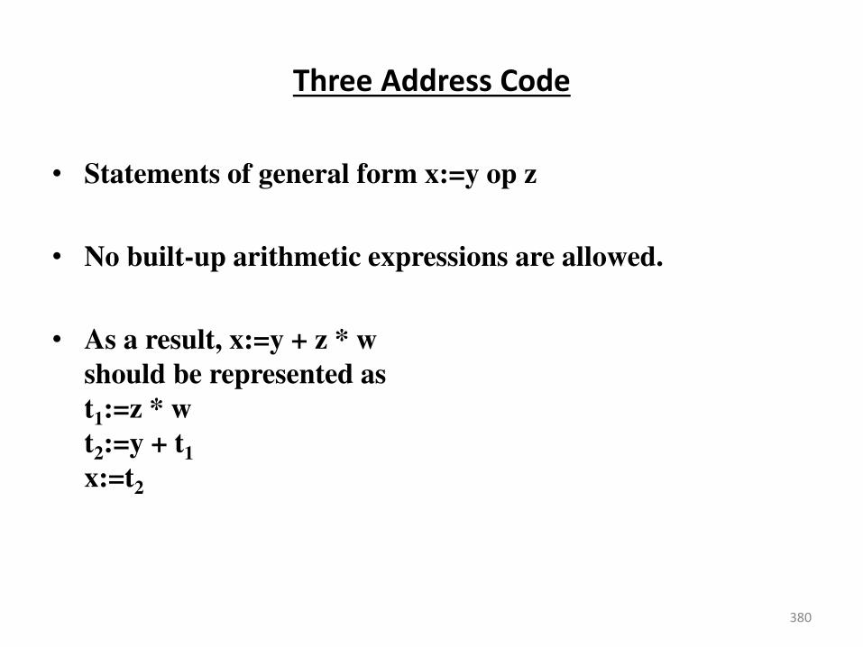
Three Address Code

• Statements of general form x:=y op z

• No built-up arithmetic expressions are allowed.

• As a result, x:=y + z * w

should be represented as

t1:=z * w

t2:=y + t1

x:=t2

380

Three Address Code

• Observe that given the syntax-tree or the dag of the

graphical representation we can easily derive a three

address code for assignments as above.

• In fact three-address code is a linearization of the tree.

• Three-address code is useful: related to machine-language/

simple/ optimizable.

381

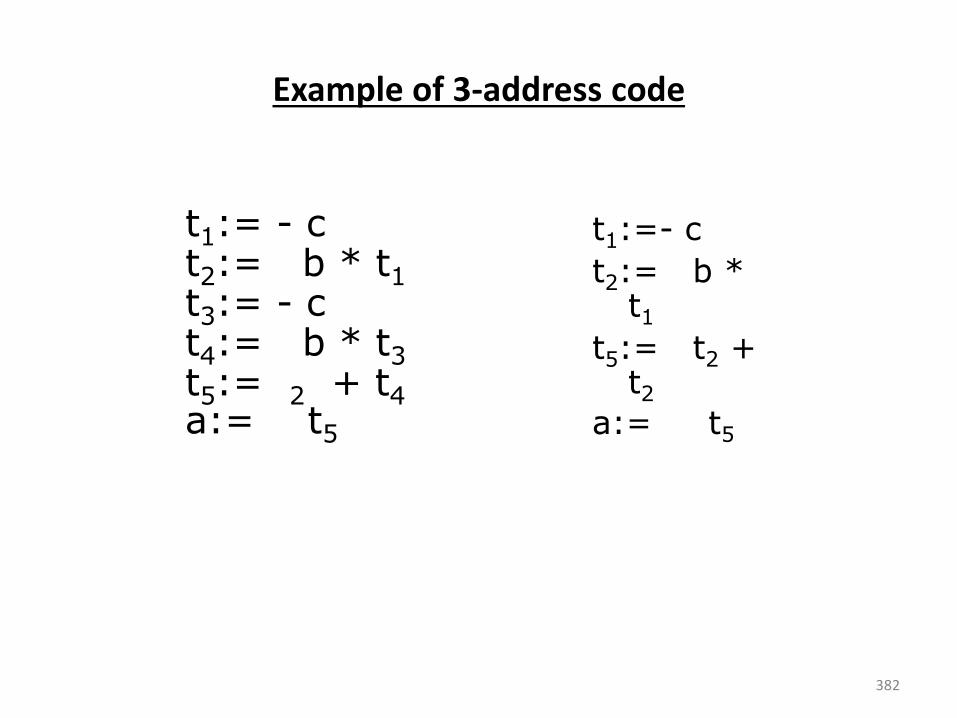
Example of 3-address code

t1:=- c

t2:= b * t1

t5:= t2 + t2

a:= t5

382

t1:= - c t2:= b * t1

t3:= - c t4:= b * t3 t5:= 2 + t4 a:= t5

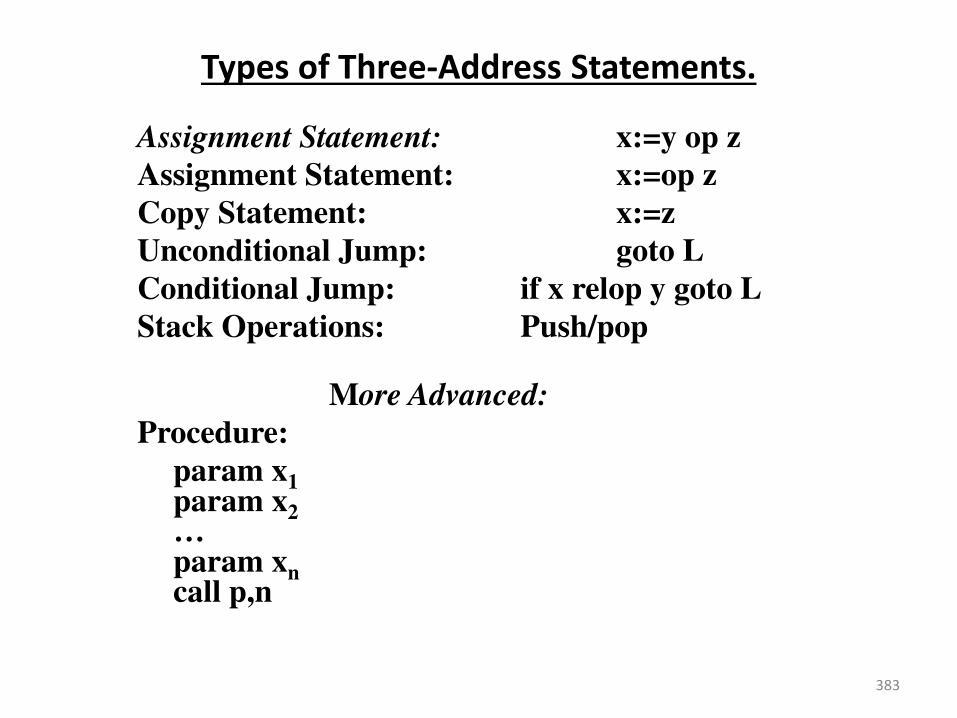
Types of Three-Address Statements.

Assignment Statement: x:=y op z Assignment Statement: x:=op z Copy Statement: x:=z Unconditional Jump: goto L Conditional Jump: if x relop y goto L Stack Operations: Push/pop

More Advanced: Procedure: param x1

param x2 … param xn call p,n

383

Types of Three-Address Statements.

Index Assignments: x:=y[i]

x[i]:=y

Address and Pointer Assignments: x:=&y

x:=*y

*x:=y

384

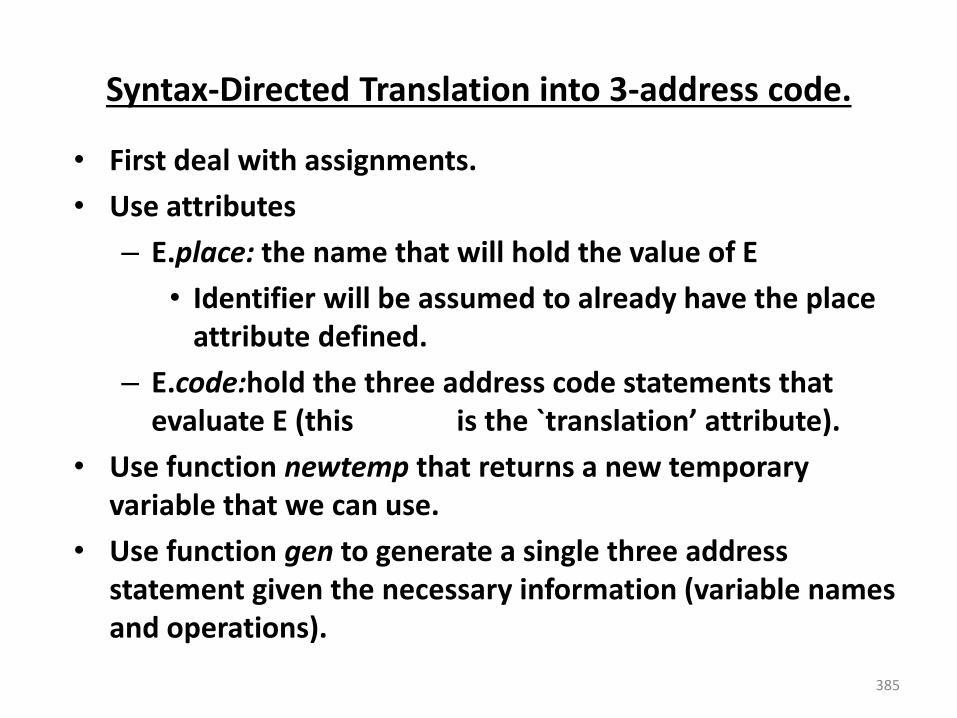
Syntax-Directed Translation into 3-address code.

• First deal with assignments.

• Use attributes

– E.place: the name that will hold the value of E

• Identifier will be assumed to already have the place

attribute defined.

– E.code:hold the three address code statements that

evaluate E (this is the `t a slatio att i ute . • Use function newtemp that returns a new temporary

variable that we can use.

• Use function gen to generate a single three address

statement given the necessary information (variable names

and operations).

385

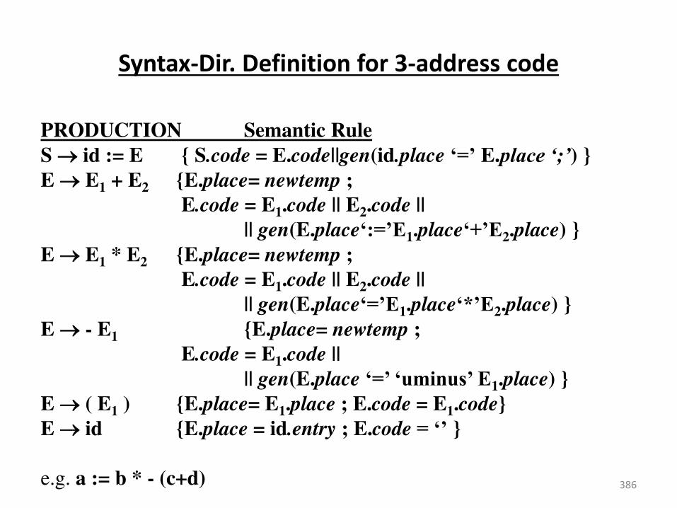
Syntax-Dir. Definition for 3-address code

PRODUCTION Semantic Rule

S id := E { S.code = E.code||gen(id.place ‘=’ E.place ‘;’) }

E E1 + E2 {E.place= newtemp ;

E.code = E1.code || E2.code ||

|| gen(E.place‘:=’E1.place‘+’E2.place) }

E E1 * E2 {E.place= newtemp ;

E.code = E1.code || E2.code ||

|| gen(E.place‘=’E1.place‘*’E2.place) }

E - E1 {E.place= newtemp ;

E.code = E1.code ||

|| gen(E.place ‘=’ ‘uminus’ E1.place) }

E ( E1 ) {E.place= E1.place ; E.code = E1.code}

E id {E.place = id.entry ; E.code = ‘’ }

e.g. a := b * - (c+d) 386

What about things that are not assignments?

• E.g. while state e ts of the for while E do “

(intepreted as while the value of E is not 0 do S)

Extension to the previous syntax-dir. Def.

PRODUCTION

S while E do S1

Semantic Rule

S.begin = newlabel;

S.after = newlabel ;

387

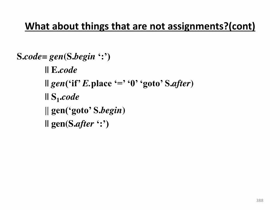
What about things that are not assignments?(cont)

S.code= gen(S.begin ‘:’) || E.code

|| gen(‘if’ E.place ‘=’ ‘0’ ‘goto’ S.after)

|| S1.code

|| gen(‘goto’ S.begin)

|| gen(S.after ‘:’)

388

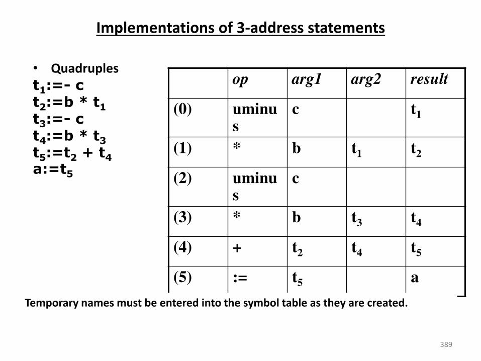
Implementations of 3-address statements

• Quadruples

t1:=- c

t2:=b * t1

t3:=- c

t4:=b * t3

t5:=t2 + t4

a:=t5

389

op arg1 arg2 result

(0) uminus

c t1

(1) * b t1 t2

(2) uminus

c

(3) * b t3 t4

(4) + t2 t4 t5

(5) := t5 a

Temporary names must be entered into the symbol table as they are created.

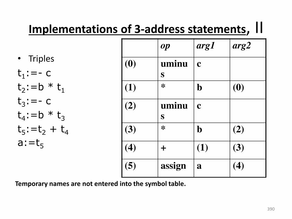
Implementations of 3-address statements, II

• Triples

t1:=- c

t2:=b * t1

t3:=- c

t4:=b * t3

t5:=t2 + t4

a:=t5

390

op arg1 arg2

(0) uminus

c

(1) * b (0)

(2) uminus

c

(3) * b (2)

(4) + (1) (3)

(5) assign a (4)

Temporary names are not entered into the symbol table.

Other types of 3-address statements

• e.g. ternary operations like

x[i]:=y x:=y[i]

• require two or more entries. e.g.

391

op arg1 arg2

(0) [ ] = x i

(1) assign (0) y

op arg1 arg2

(0) [ ] = y i

(1) assign x (0)

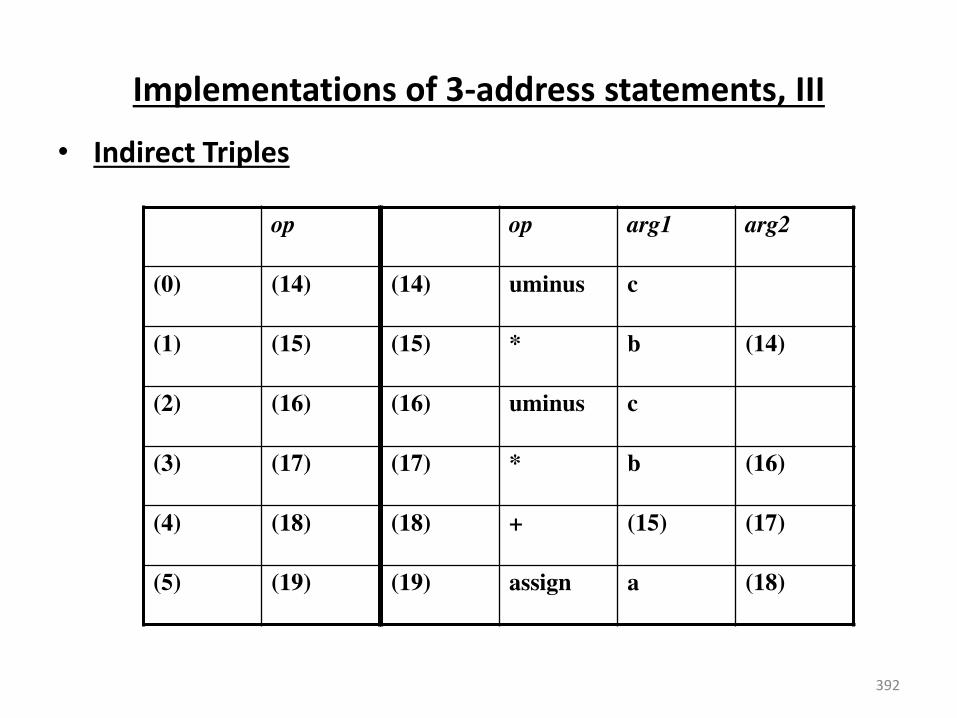
Implementations of 3-address statements, III

• Indirect Triples

392

op arg1 arg2

(14) uminus c

(15) * b (14)

(16) uminus c

(17) * b (16)

(18) + (15) (17)

(19) assign a (18)

op

(0) (14)

(1) (15)

(2) (16)

(3) (17)

(4) (18)

(5) (19)

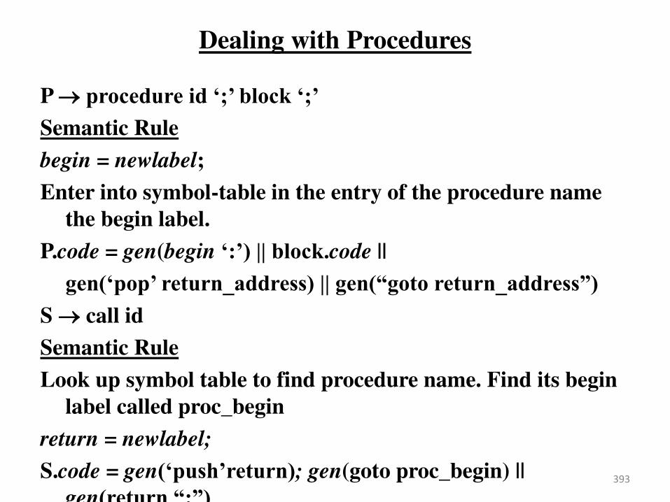
Dealing with Procedures

P procedure id ‘;’ block ‘;’

Semantic Rule

begin = newlabel;

Enter into symbol-table in the entry of the procedure name

the begin label.

P.code = gen(begin ‘:’) || block.code ||

gen(‘pop’ return_address) || gen(“goto return_address”) S call id

Semantic Rule

Look up symbol table to find procedure name. Find its begin

label called proc_begin

return = newlabel;

S.code = gen(‘push’return); gen(goto proc_begin) ||

gen(return “:”) 393

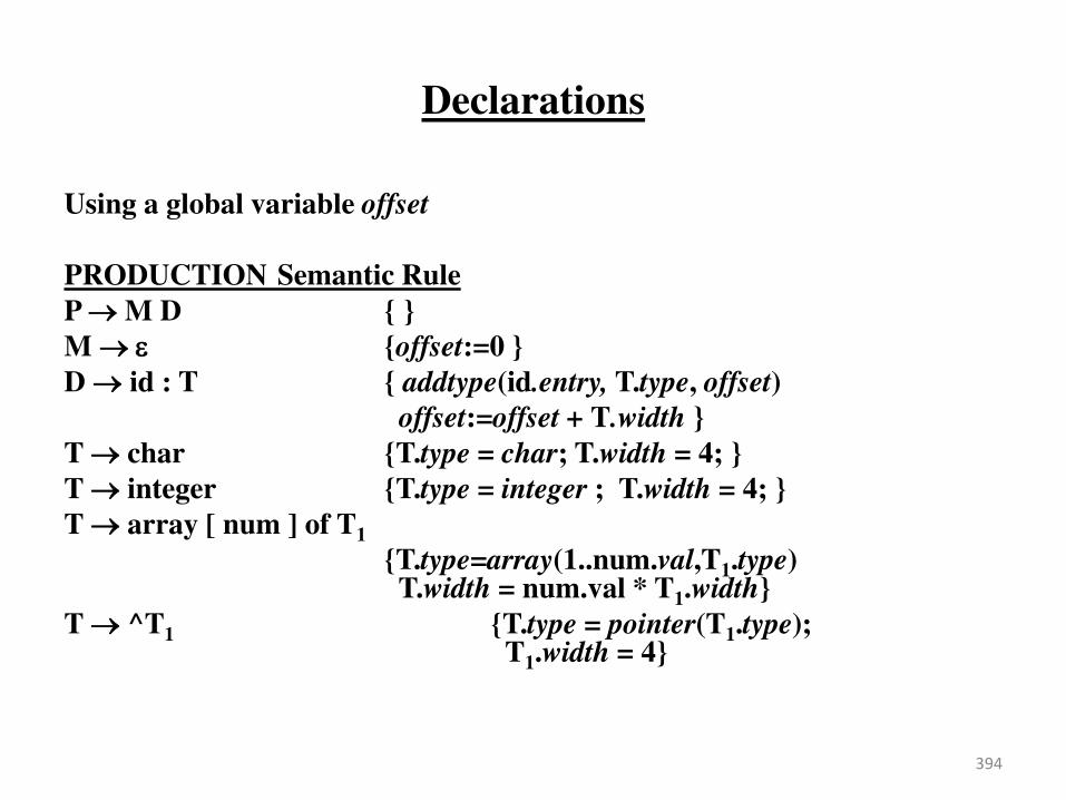
Declarations

Using a global variable offset

PRODUCTION Semantic Rule

P M D { }

M {offset:=0 }

D id : T { addtype(id.entry, T.type, offset) offset:=offset + T.width }

T char {T.type = char; T.width = 4; }

T integer {T.type = integer ; T.width = 4; }

T array [ num ] of T1 {T.type=array(1..num.val,T1.type)

T.width = num.val * T1.width}

T ^T1 {T.type = pointer(T1.type); T1.width = 4}

394

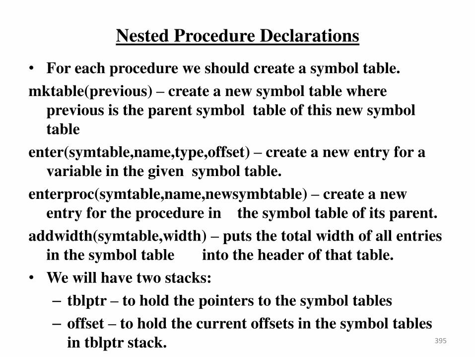
Nested Procedure Declarations

• For each procedure we should create a symbol table.

mktable(previous) – create a new symbol table where

previous is the parent symbol table of this new symbol

table

enter(symtable,name,type,offset) – create a new entry for a

variable in the given symbol table.

enterproc(symtable,name,newsymbtable) – create a new

entry for the procedure in the symbol table of its parent.

addwidth(symtable,width) – puts the total width of all entries

in the symbol table into the header of that table.

• We will have two stacks:

– tblptr – to hold the pointers to the symbol tables

– offset – to hold the current offsets in the symbol tables

in tblptr stack.

395

Keeping Track of Scope Information

Consider the grammar fraction:

P D

D D ; D | id : T | proc id ; D ; S

Each procedure should be allowed to use independent names.

Nested procedures are allowed.

396

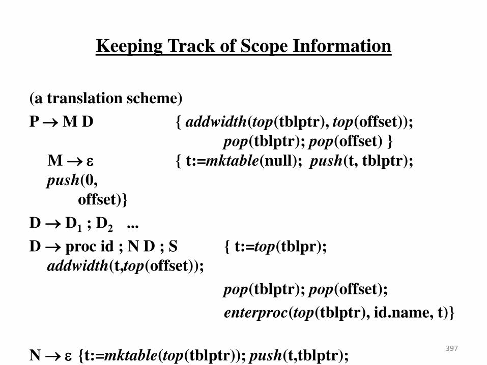
Keeping Track of Scope Information

(a translation scheme)

P M D { addwidth(top(tblptr), top(offset)); pop(tblptr); pop(offset) }

M { t:=mktable(null); push(t, tblptr);

push(0,

offset)}

D D1 ; D2 ...

D proc id ; N D ; S { t:=top(tblpr);

addwidth(t,top(offset));

pop(tblptr); pop(offset);

enterproc(top(tblptr), id.name, t)}

N {t:=mktable(top(tblptr)); push(t,tblptr);

push(0,offset);}

397

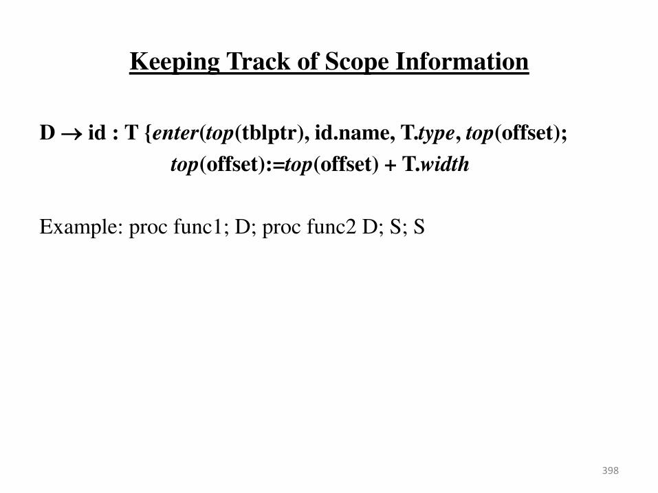
Keeping Track of Scope Information

D id : T {enter(top(tblptr), id.name, T.type, top(offset);

top(offset):=top(offset) + T.width

Example: proc func1; D; proc func2 D; S; S

398

Type Checking

. 399

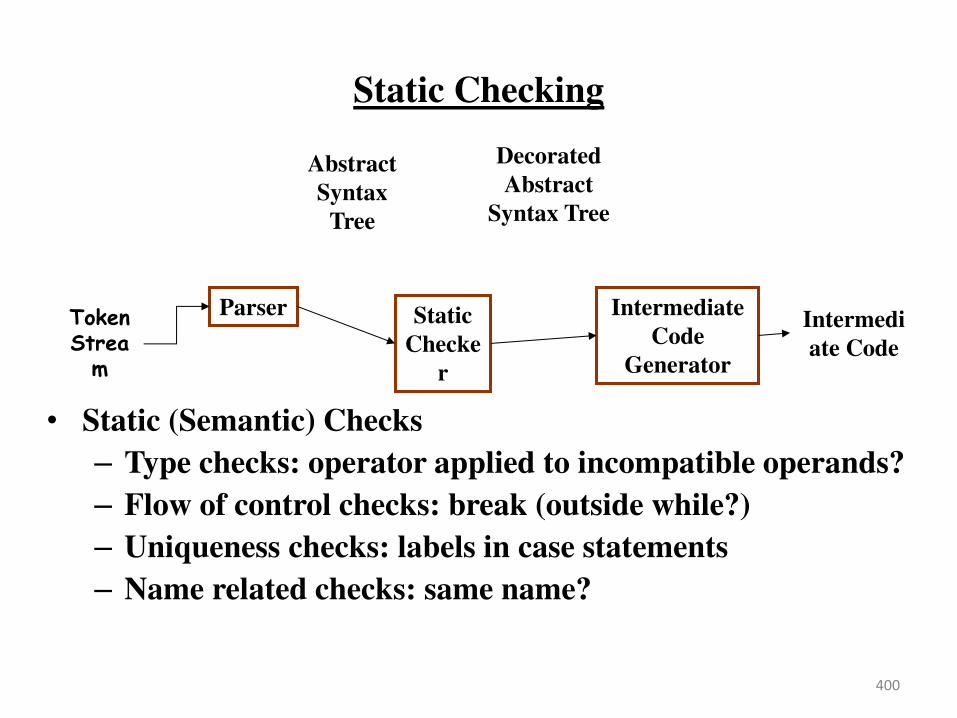
Static Checking

• Static (Semantic) Checks

– Type checks: operator applied to incompatible operands?

– Flow of control checks: break (outside while?)

– Uniqueness checks: labels in case statements

– Name related checks: same name?

400

Token Strea

m

Parser Static

Checke

r

Intermediate

Code

Generator

Abstract

Syntax

Tree

Decorated

Abstract

Syntax Tree

Intermedi

ate Code

Type Checking

• Problem: Verify that a type of a construct matches that expected by its context.

• Examples:

– mod requires integer operands (PASCAL)

– * (dereferencing) – applied to a pointer

– a[i] – indexing applied to an array

– f(a1, aβ, …, an) – function applied to correct arguments.

• Information gathered by a type checker:

– Needed during code generation.

401

Type Systems

• A collection of rules for assigning type expressions to the various parts of a program.

• Based on: Syntactic constructs, notion of a type.

• Example: If both operators of “+”, “-”, “*” are of type integer then so is the result.

• Type Checker: An implementation of a type system.

– Syntax Directed.

• Sound Type System: eliminates the need for checking type errors during run time.

402

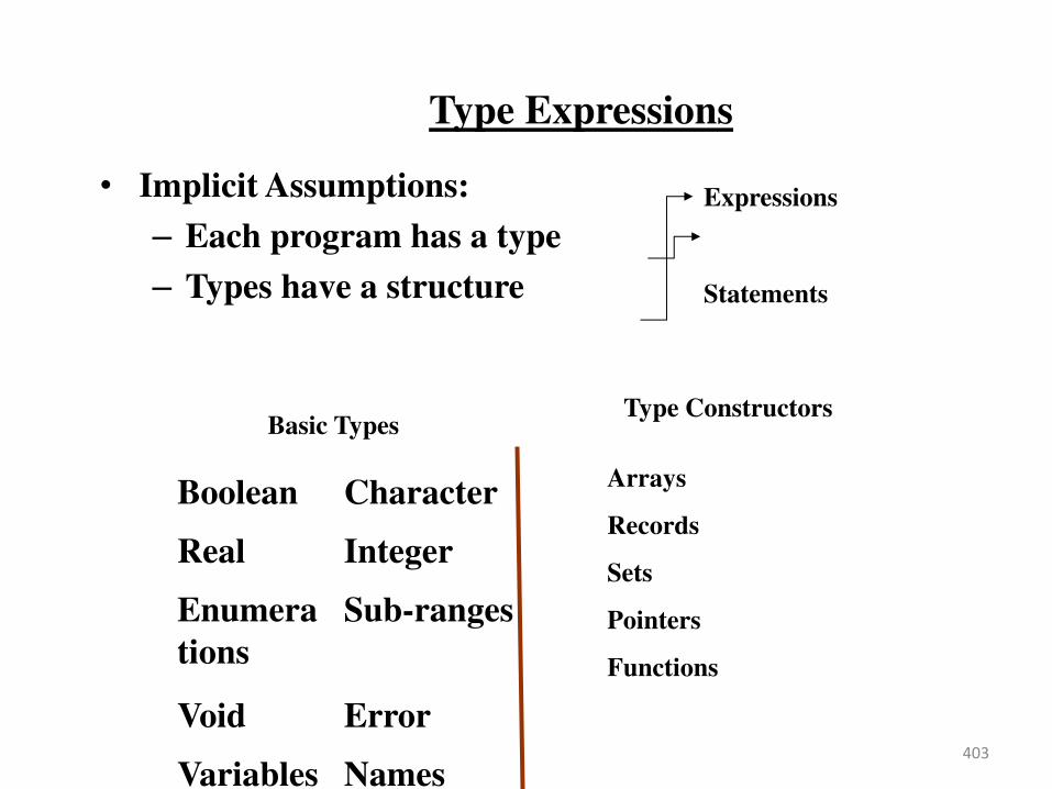
Type Expressions

• Implicit Assumptions:

– Each program has a type

– Types have a structure

Boolean Character

Real Integer

Enumera

tions

Sub-ranges

Void Error

Variables Names 403

Basic Types Type Constructors

Arrays

Records

Sets

Pointers

Functions

Expressions

Statements

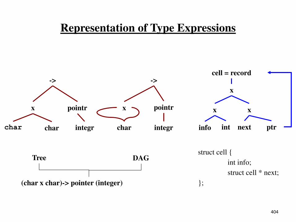
Representation of Type Expressions

404

->

x pointr

char char

(char x char)-> pointer (integer)

integr

->

x pointr

integr char

Tree DAG struct cell {

int info;

struct cell * next;

};

cell = record

x

x x

info int next ptr

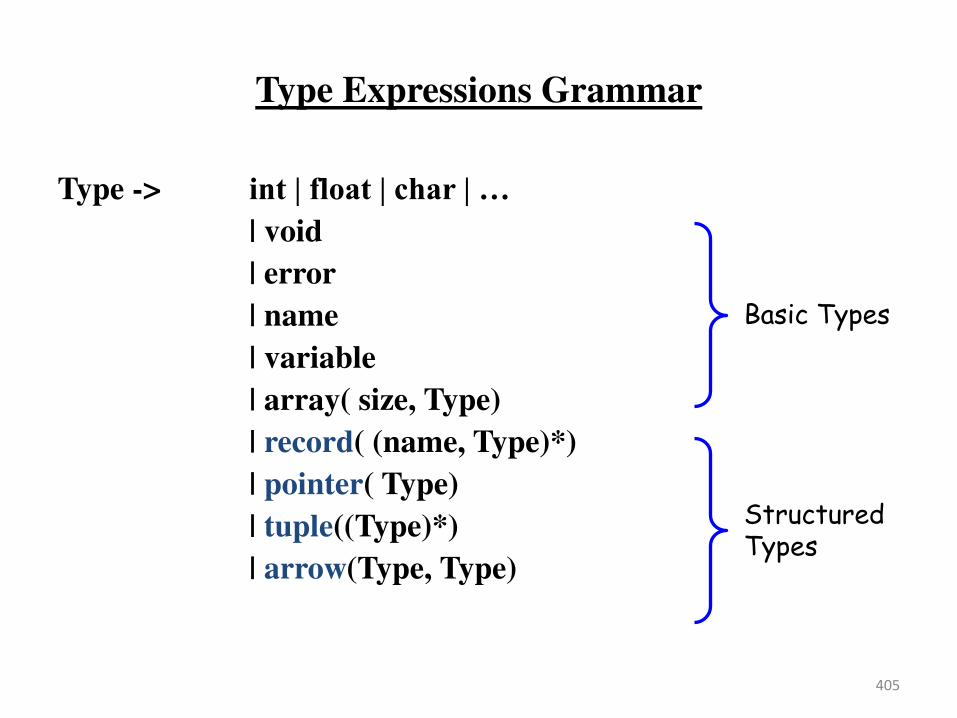
Type Expressions Grammar

Type -> int | float | char | …

| void

| error

| name

| variable

| array( size, Type)

| record( (name, Type)*)

| pointer( Type)

| tuple((Type)*)

| arrow(Type, Type)

405

Basic Types

Structured Types

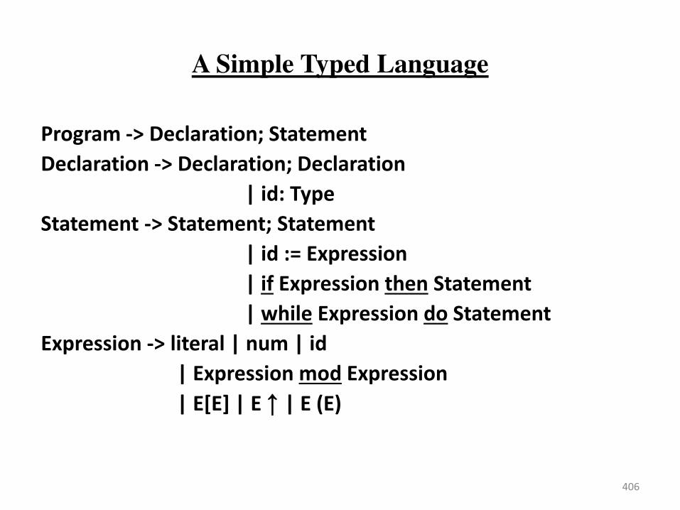
A Simple Typed Language

Program -> Declaration; Statement

Declaration -> Declaration; Declaration

| id: Type

Statement -> Statement; Statement

| id := Expression

| if Expression then Statement

| while Expression do Statement

Expression -> literal | num | id

| Expression mod Expression

| E[E] | E ↑ | E (E)

406

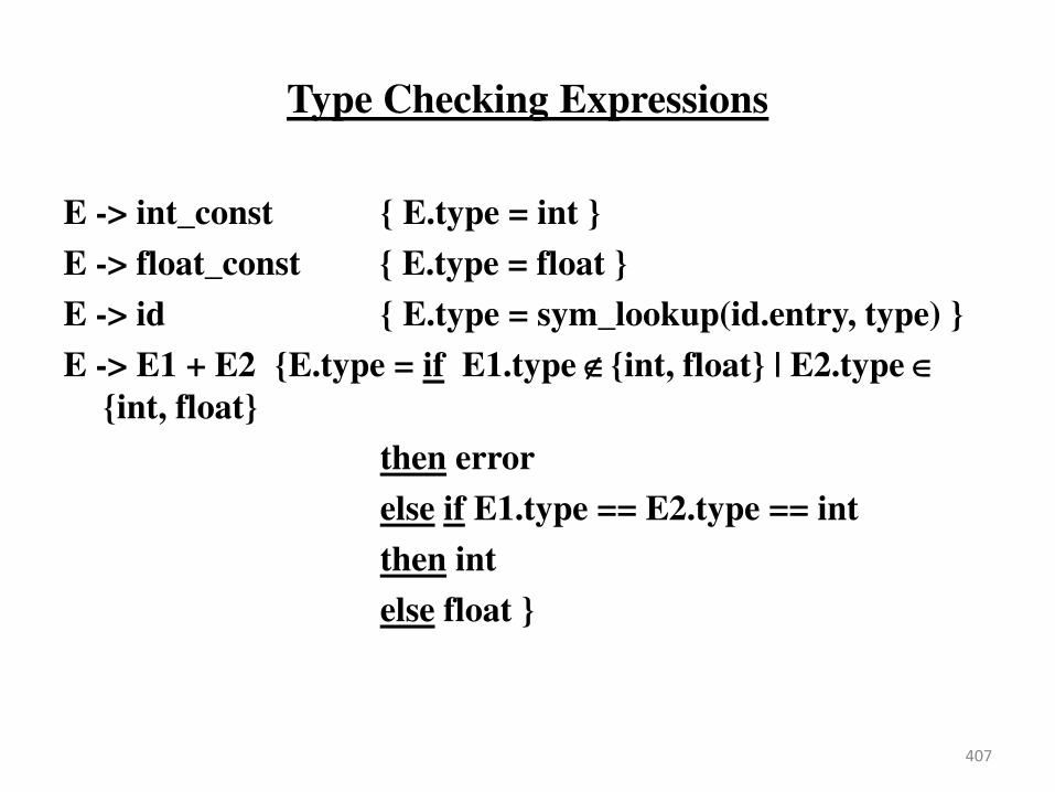
Type Checking Expressions

E -> int_const { E.type = int }

E -> float_const { E.type = float }

E -> id { E.type = sym_lookup(id.entry, type) }

E -> E1 + E2 {E.type = if E1.type {int, float} | E2.type

{int, float}

then error

else if E1.type == E2.type == int

then int

else float }

407

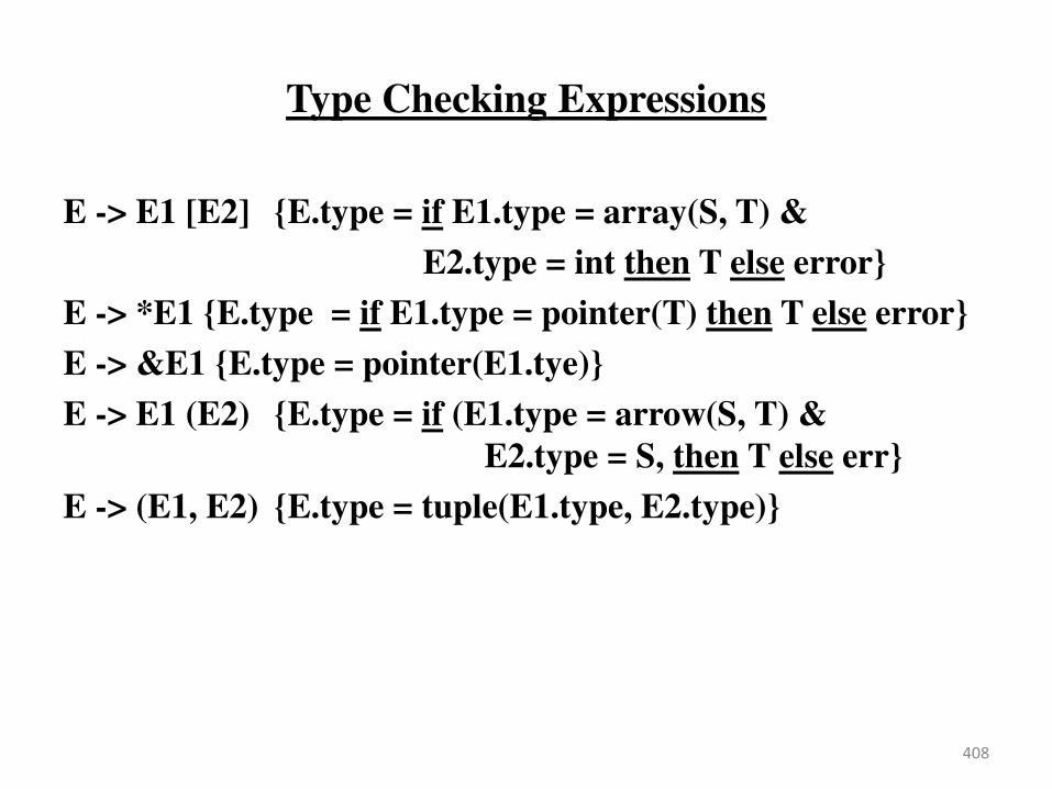
Type Checking Expressions

E -> E1 [E2] {E.type = if E1.type = array(S, T) &

E2.type = int then T else error}

E -> *E1 {E.type = if E1.type = pointer(T) then T else error}

E -> &E1 {E.type = pointer(E1.tye)}

E -> E1 (E2) {E.type = if (E1.type = arrow(S, T) &

E2.type = S, then T else err}

E -> (E1, E2) {E.type = tuple(E1.type, E2.type)}

408

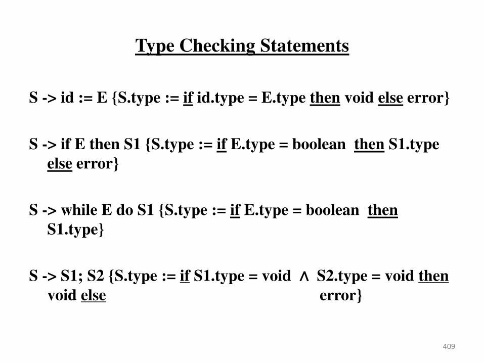
Type Checking Statements

S -> id := E {S.type := if id.type = E.type then void else error}

S -> if E then S1 {S.type := if E.type = boolean then S1.type

else error}

S -> while E do S1 {S.type := if E.type = boolean then

S1.type}

S -> S1; S2 {S.type := if S1.type = void ∧ S2.type = void then

void else error}

409

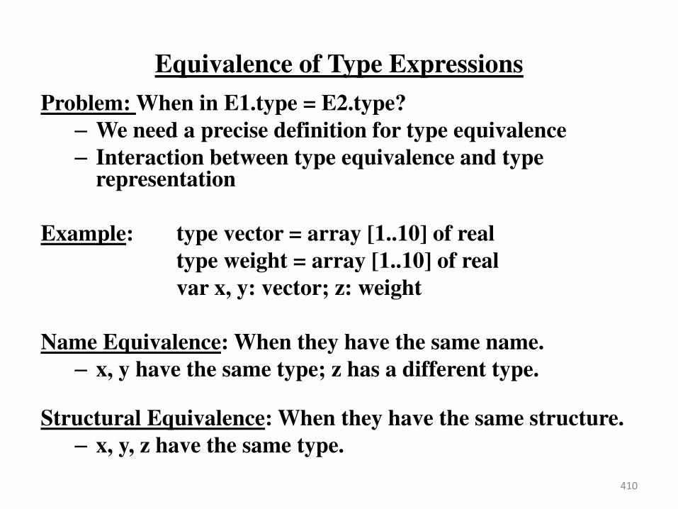
Equivalence of Type Expressions

Problem: When in E1.type = E2.type?

– We need a precise definition for type equivalence

– Interaction between type equivalence and type representation

Example: type vector = array [1..10] of real

type weight = array [1..10] of real

var x, y: vector; z: weight

Name Equivalence: When they have the same name.

– x, y have the same type; z has a different type.

Structural Equivalence: When they have the same structure.

– x, y, z have the same type.

410

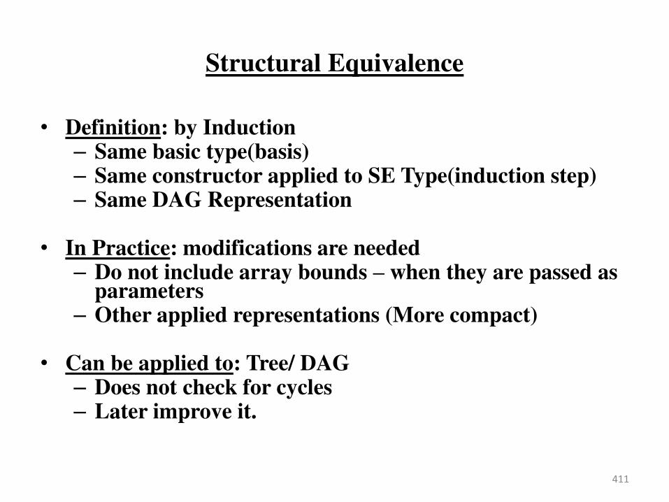
Structural Equivalence

• Definition: by Induction – Same basic type(basis) – Same constructor applied to SE Type(induction step) – Same DAG Representation

• In Practice: modifications are needed

– Do not include array bounds – when they are passed as parameters

– Other applied representations (More compact)

• Can be applied to: Tree/ DAG – Does not check for cycles – Later improve it.

411

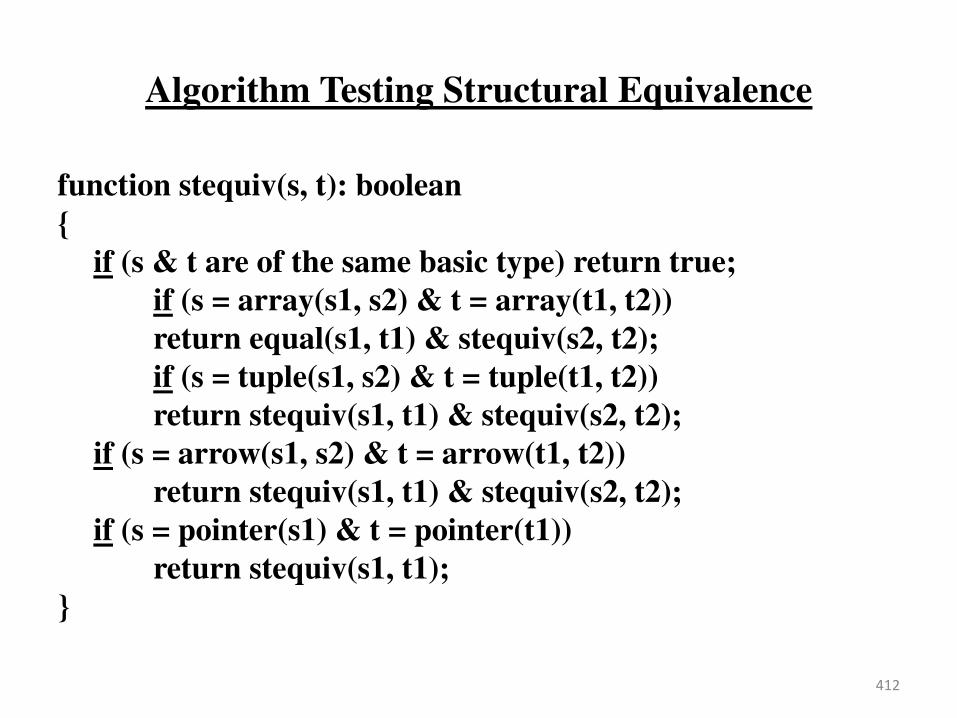
Algorithm Testing Structural Equivalence

function stequiv(s, t): boolean

{

if (s & t are of the same basic type) return true;

if (s = array(s1, s2) & t = array(t1, t2))

return equal(s1, t1) & stequiv(s2, t2);

if (s = tuple(s1, s2) & t = tuple(t1, t2))

return stequiv(s1, t1) & stequiv(s2, t2);

if (s = arrow(s1, s2) & t = arrow(t1, t2))

return stequiv(s1, t1) & stequiv(s2, t2);

if (s = pointer(s1) & t = pointer(t1))

return stequiv(s1, t1);

}

412

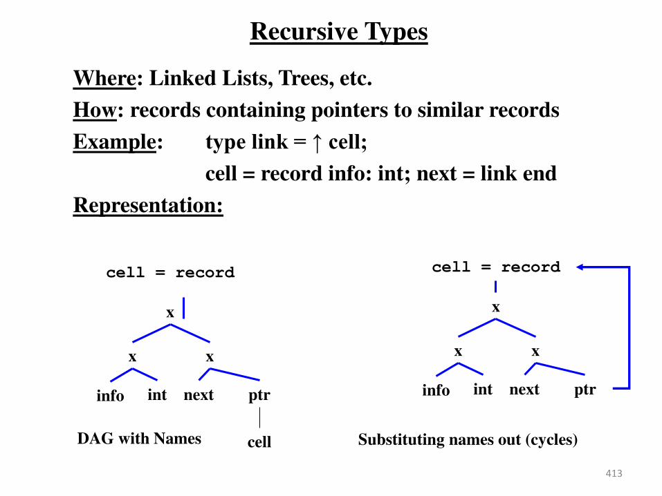
Recursive Types

Where: Linked Lists, Trees, etc.

How: records containing pointers to similar records

Example: type link = cell; cell = record info: int; next = link end

Representation:

413

cell = record

x

x x

info int next ptr

cell = record

x

x x

info int next ptr

cell DAG with Names Substituting names out (cycles)

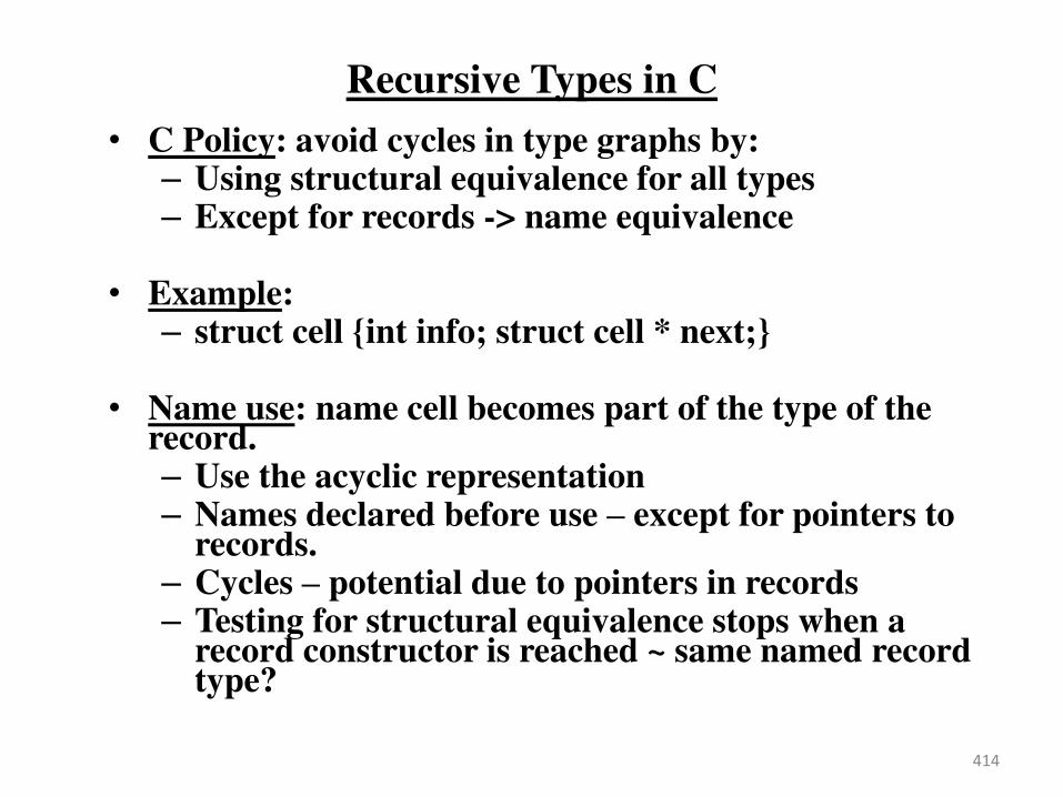
Recursive Types in C

• C Policy: avoid cycles in type graphs by: – Using structural equivalence for all types – Except for records -> name equivalence

• Example: – struct cell {int info; struct cell * next;}

• Name use: name cell becomes part of the type of the

record. – Use the acyclic representation – Names declared before use – except for pointers to

records. – Cycles – potential due to pointers in records – Testing for structural equivalence stops when a

record constructor is reached ~ same named record type?

414

Overloading Functions & Operators

• Overloaded Symbol: one that has different meanings depending on its context

• Example: Addition operator +

• Resolving (operator identification): overloading is resolved when a unique meaning is determined.

• Context: it is not always possible to resolve overloading by looking only the arguments of a function

– Set of possible types

– Context (inherited attribute) necessary

415

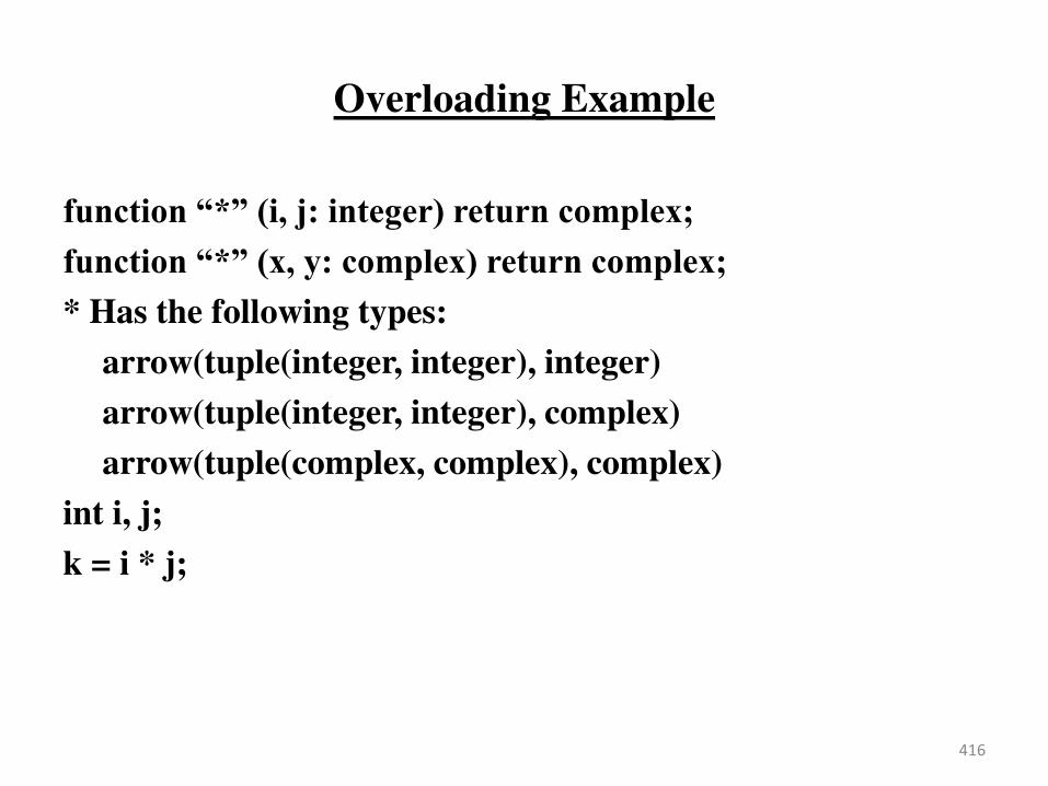
Overloading Example

function “*” (i, j: integer) return complex; function “*” (x, y: complex) return complex; * Has the following types:

arrow(tuple(integer, integer), integer)

arrow(tuple(integer, integer), complex)

arrow(tuple(complex, complex), complex)

int i, j;

k = i * j;

416

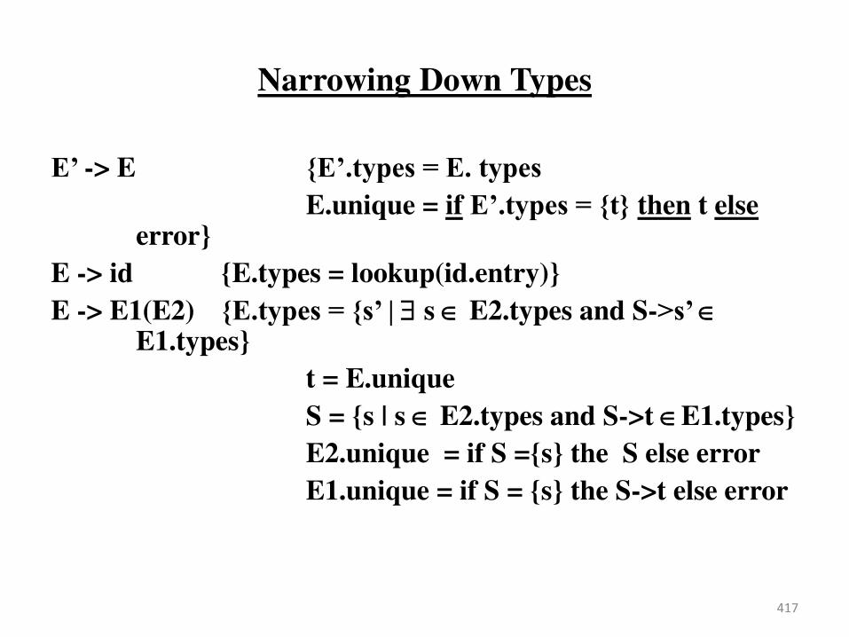
Narrowing Down Types

E’ -> E {E’.types = E. types

E.unique = if E’.types = {t} then t else error}

E -> id {E.types = lookup(id.entry)}

E -> E1(E2) {E.types = {s’ | s E2.types and S->s’ E1.types}

t = E.unique

S = {s | s E2.types and S->t E1.types}

E2.unique = if S ={s} the S else error

E1.unique = if S = {s} the S->t else error

417

Polymorphic Functions

• Defn: a piece of code (functions, operators) that can be executed with arguments of different types.

• Examples: Built in Operator indexing arrays, pointer manipulation

• Why use them: facilitate manipulation of data structures regardless of types.

• Example HL:

fun length(lptr) = if null (lptr) then 0

else length(+l(lptr)) + 1

418

A Language for Polymorphic Functions

P -> D ; E

D -> D ; D | id : Q

Q -> α. Q | T

T -> arrow (T, T) | tuple (T, T)

| unary (T) | (T)

| basic

| α

E -> E (E) | E, E | id

419

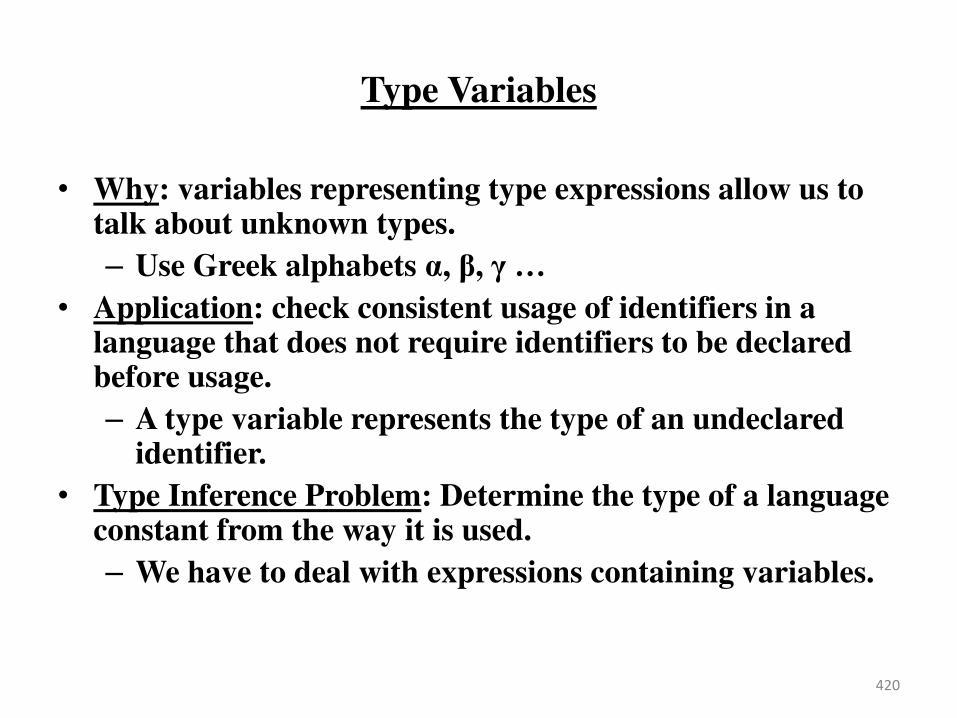
Type Variables

• Why: variables representing type expressions allow us to talk about unknown types.

– Use Greek alphabets α, , …

• Application: check consistent usage of identifiers in a language that does not require identifiers to be declared before usage.

– A type variable represents the type of an undeclared identifier.

• Type Inference Problem: Determine the type of a language constant from the way it is used.

– We have to deal with expressions containing variables.

420

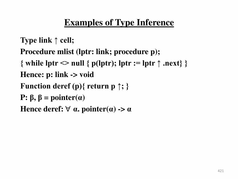
Examples of Type Inference

Type link cell; Procedure mlist (lptr: link; procedure p);

{ while lptr <> null { p(lptr); lptr := lptr .next} }

Hence: p: link -> void

Function deref (p){ return p ; }

P: , = pointer(α)

Hence deref: α. pointer(α) -> α

421

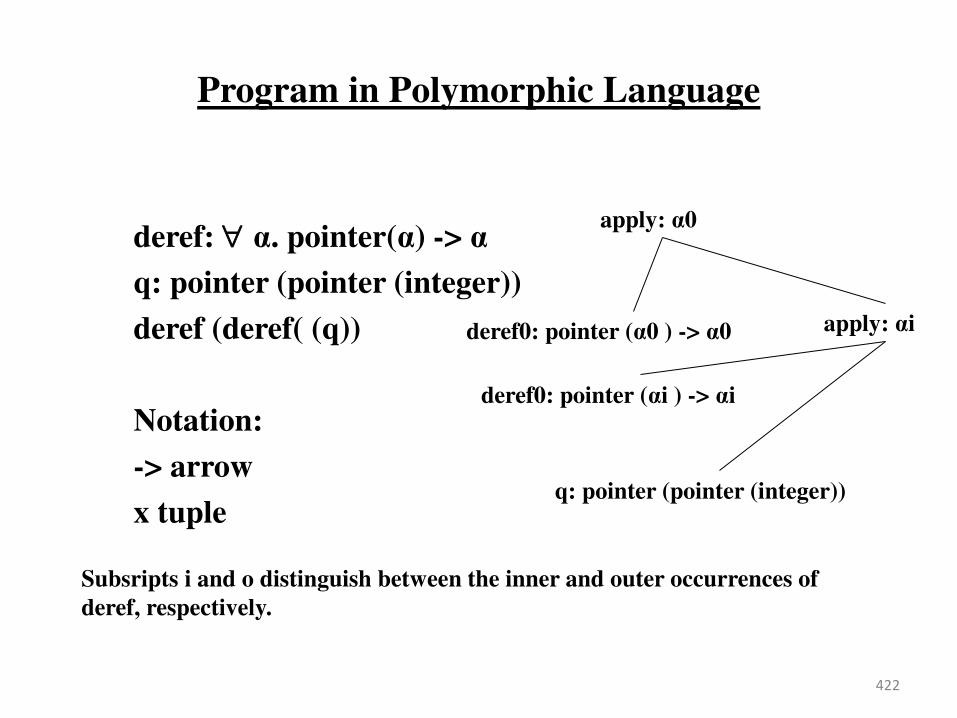
Program in Polymorphic Language

deref: α. pointer(α) -> α

q: pointer (pointer (integer))

deref (deref( (q))

Notation:

-> arrow

x tuple

422

apply: α0

deref0: pointer (α0 ) -> α0 apply: αi

deref0: pointer (αi ) -> αi

q: pointer (pointer (integer))

Subsripts i and o distinguish between the inner and outer occurrences of

deref, respectively.

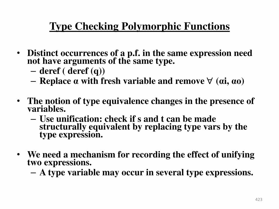
Type Checking Polymorphic Functions

• Distinct occurrences of a p.f. in the same expression need not have arguments of the same type. – deref ( deref (q)) – Replace α with fresh variable and remove (αi, αo)

• The notion of type equivalence changes in the presence of variables. – Use unification: check if s and t can be made

structurally equivalent by replacing type vars by the type expression.

• We need a mechanism for recording the effect of unifying two expressions. – A type variable may occur in several type expressions.

423

Substitutions and Unification

• Substitution: a mapping from type variables to type expressions.

Function subst (t: type Expr): type Expr { S

if (t is a basic type) return t;

if (t is a basic variable) return S(t); --identify if t S

if (t is t1 -> t2) return subst(t1) -> subst (t2); }

• Instance: S(t) is an instance of t written S(t) < t.

– Examples: pointer (integer) < pointer (α) , int -> real ≠ α-> α

• Unify: t1 ≈ tβ if S. S (t1) = S (t2)

• Most General Unifier S: A substitution S:

– S (t1) = S (t2)

– S’. S’ (t1) = S’ (tβ) t. S’(t) < S(t).

424

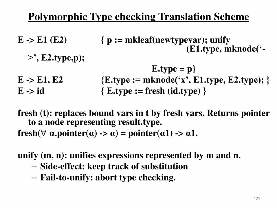
Polymorphic Type checking Translation Scheme

E -> E1 (E2) { p := mkleaf(newtypevar); unify (E1.type, mknode(‘->’, Eβ.type,p);

E.type = p}

E -> E1, E2 {E.type := mknode(‘x’, E1.type, Eβ.type); }

E -> id { E.type := fresh (id.type) }

fresh (t): replaces bound vars in t by fresh vars. Returns pointer to a node representing result.type.

fresh( α.pointer(α) -> α) = pointer(α1) -> α1.

unify (m, n): unifies expressions represented by m and n.

– Side-effect: keep track of substitution

– Fail-to-unify: abort type checking.

425

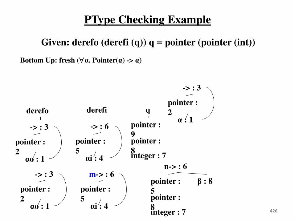
PType Checking Example

Given: derefo (derefi (q)) q = pointer (pointer (int))

426

Bottom Up: fresh (α. Pointer(α) -> α)

-> : 3

pointer :

2 α : 1

-> : 3

pointer :

2 αo : 1

derefo

-> : 6

pointer :

5 αi : 4

derefi q

pointer :

9 pointer :

8 integer : 7

-> : 3

pointer :

2 αo : 1

m-> : 6

pointer :

5 αi : 4

pointer :

5 pointer :

8 integer : 7

n-> : 6

: 8

UNIT-3

PART-B

SYMBOL TABLE

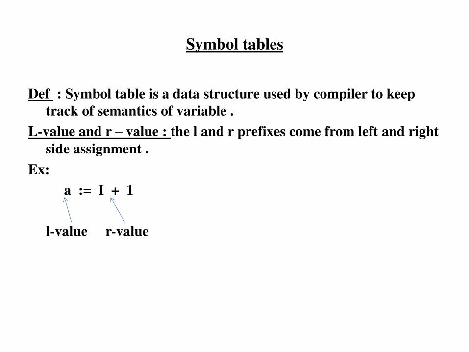
Symbol tables

Def : Symbol table is a data structure used by compiler to keep

track of semantics of variable .

L-value and r – value : the l and r prefixes come from left and right

side assignment .

Ex:

a := I + 1

l-value r-value

Symbol table entries

• Variable names

• Constants

• Procedure names

• Function names

• Literal constants and strings

• Compiler generated temporaries

• Labels in source languages

Compiler uses following types of information from symbol table

1.Data type

2.Name

3.Declaring procedures

4.Offset in storage

Symbol table entries

5.If structure are record then pointer to structure variable .

6.For parameters, whether parameter passing is

by value or reference .

7.Number and type of arguments passed to the function .

8.Base address .

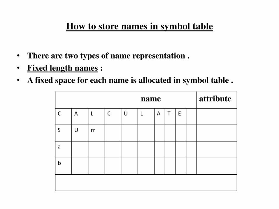
How to store names in symbol table

• There are two types of name representation .

• Fixed length names :

• A fixed space for each name is allocated in symbol table .

name attribute

C A L C U L A T E

S U m

a

b

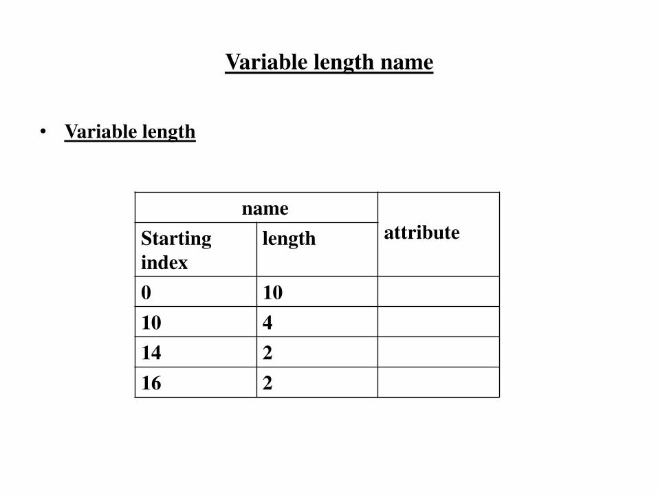
Variable length name

• Variable length

name

attribute Starting

index

length

0 10

10 4

14 2

16 2

Symbol table management

• Data structure for symbol table :

1 . Linear list

2 . Arrays

The pointer variable is maintained at the end of all stored records .

Name 1 Info 1

Name2 Info 2

Name 3 Info 3

.

.

.

.

.

.

Name n Info n Available

(start of empty

slot

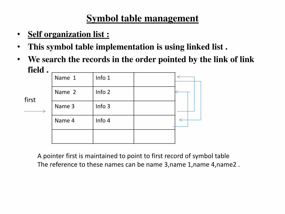
Symbol table management

• Self organization list :

• This symbol table implementation is using linked list .

• We search the records in the order pointed by the link of link

field .

Name 1 Info 1

Name 2 Info 2

Name 3 Info 3

Name 4 Info 4

first

A pointer first is maintained to point to first record of symbol table

The reference to these names can be name 3,name 1,name 4,name2 .

Symbol table management

• Self organization list :

• When the name is referenced or created it is moved to the front of

the list .

• The most frequently referred names will tend to be front of the list .

Hence access time to most frequently referred names will be the

least .

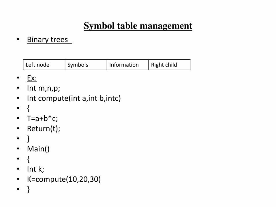
Symbol table management

• Binary trees

• Ex:

• Int m,n,p;

• Int compute(int a,int b,intc)

• {

• T=a+b*c;

• Return(t);

• }

• Main()

• {

• Int k;

• K=compute(10,20,30)

• }

Left node Symbols Information Right child

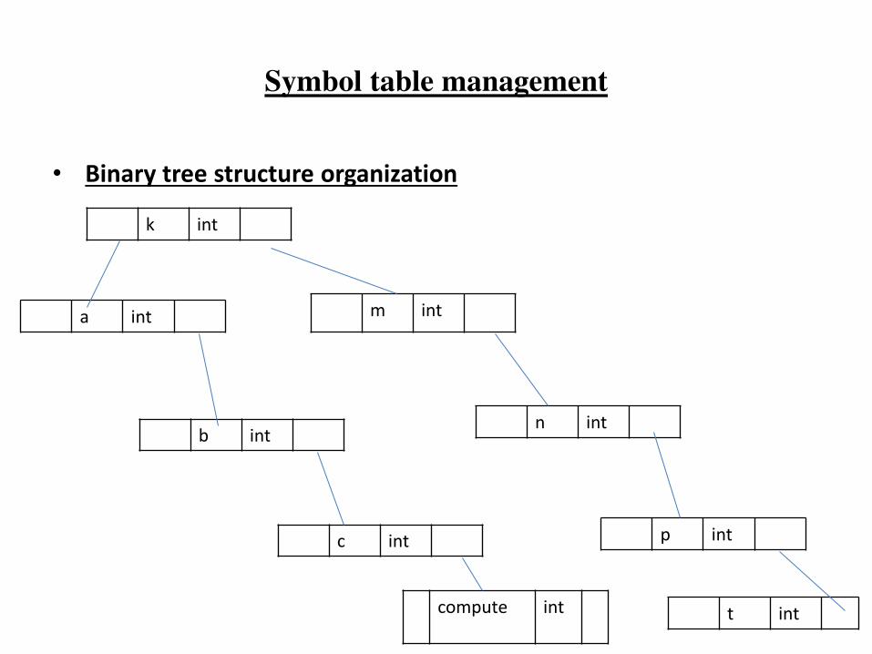
Symbol table management

• Binary tree structure organization

k int

m int a int

b int n int

c int p int

compute int t int

Symbol table management

• Binary tree structure organization

• Advantages :

• Insertion of any symbol is efficient.

• Any symbol can be searched efficiently using binary searching

method.

• Disadvantages :

• This structure consumes lot of space in storing left pointer,right

pointer and null pointers.

Symbol table management

• Hash tables :

• It is used to search the records of symbol table .

• In hashing two tables are maintained a hash table and symbol table .

• Hash table contains of k entries from 0,1 to k-1 . These entries are basically pointers to symbol table pointing to the names of symbol table .

• To determine where the name is in symbol table ,we use a hash function ‘h’ such that h(name) will result any integer between 0 to k-1 . We can search any name by

position = h(name)

Using this position we can obtain the exact locations of name in symbol table .

Symbol table management

• Hash tables :

The hash function should result in uniform distribution of names

in symbol table .

The hash function should be such that there will be minimum

number of collision . Collision is such a situation where hash

function results in same location for storing the names .

Various collision resolution techniques are open addressing,

chaining , rehashing .

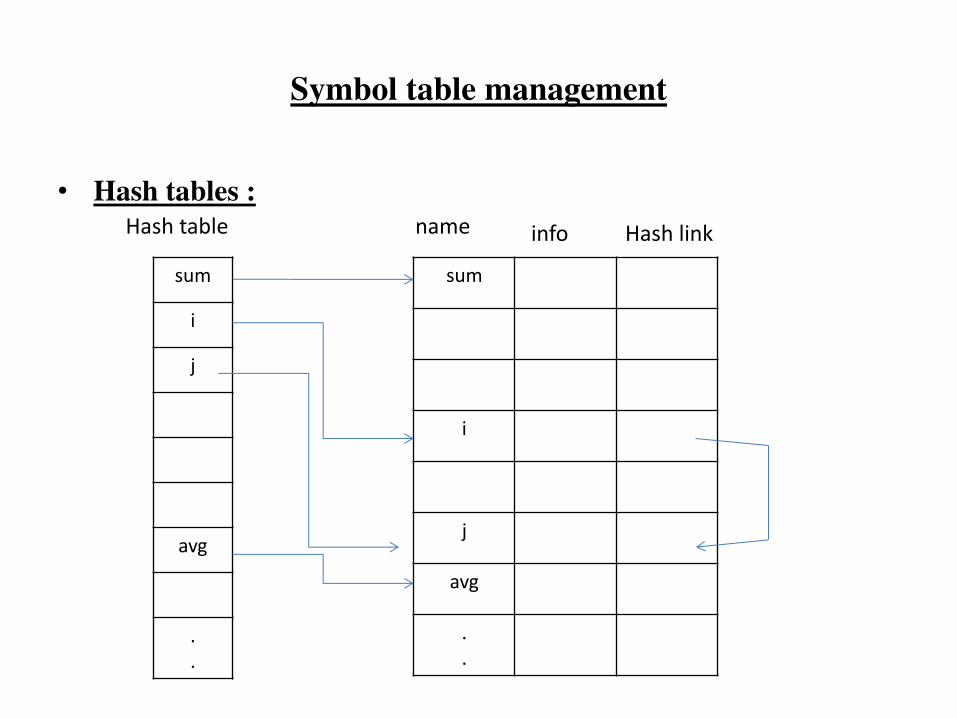
Symbol table management

• Hash tables :

sum

i

j

avg

.

.

Hash table

sum

i

j

avg

.

.

name info Hash link

Symbol table management

• Hash tables :

• The advantages of hash table is quick search is possible .

• The disadvantage is that hashing is complicated to implement .

Some extra space is required . Obtaining scope of variables is

very difficult .

Symbol table management

• HEAP ALLOCATION:

• The stack allocation strategy cannot be used if either of the following is possible:

• 1. The values of local names must be retained when activation ends.

• 2. A called activation outlives the caller.

•

• In each of the above cases, the deallocation of activation records need not occur in a last- in first-out fashion, so storage cannot be organized as a stack.

• Heap allocation parcels out pieces contiguous storage, as needed for activation records or other objects. Pieces may be deallocated in any order, so over time the heap will consist of alternate areas that are free and in use.

Storage allocation stratagies

• 1.code area

• 2.Static data area

• 3.Stack area

• 4.heap area

• There are 3 different storage allocation strategies based on this

division of run time storage .the strategies are

• 1.Static allocation :At compile time

• 2.Stack allocation : A stack is used to manage the run time

manage .

• 3 . Heap allocation : heap is used to manage the dynamic

memory allocation .

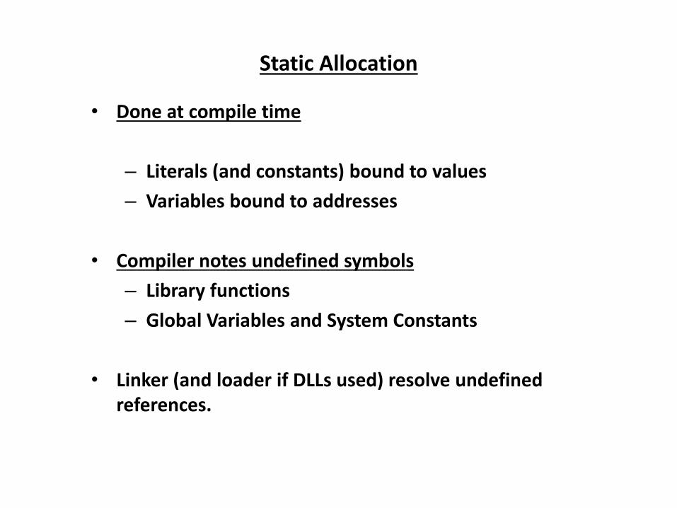
Static Allocation

• Done at compile time

– Literals (and constants) bound to values

– Variables bound to addresses

• Compiler notes undefined symbols

– Library functions

– Global Variables and System Constants

• Linker (and loader if DLLs used) resolve undefined

references.

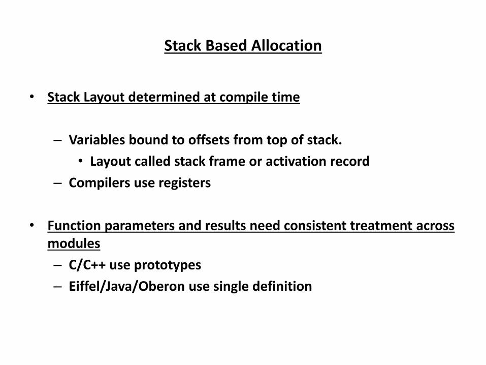
Stack Based Allocation

• Stack Layout determined at compile time

– Variables bound to offsets from top of stack.

• Layout called stack frame or activation record

– Compilers use registers

• Function parameters and results need consistent treatment across

modules

– C/C++ use prototypes

– Eiffel/Java/Oberon use single definition

Heap Allocation

• Heap provides dynamic memory management.

– Not to be confused with binary heap or binomial

heap data structures.

– Under the hood, may periodically need to request

additional memory from the O/S.

• Requested large regions (requests are

expensive).

– Done using a library (e.g. C)

– Or as part of the language (C++, Java, Lisp).

Activation Record

model of Activation Record

Return value

Actual parameters

Control link(dynamic link)

Access link (static link)

Saved machine status

Local variables

Temporaries

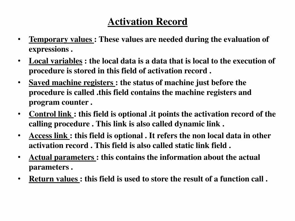
Activation Record • Temporary values : These values are needed during the evaluation of

expressions .

• Local variables : the local data is a data that is local to the execution of

procedure is stored in this field of activation record .

• Saved machine registers : the status of machine just before the

procedure is called .this field contains the machine registers and

program counter .

• Control link : this field is optional .it points the activation record of the

calling procedure . This link is also called dynamic link .

• Access link : this field is optional . It refers the non local data in other

activation record . This field is also called static link field .

• Actual parameters : this contains the information about the actual

parameters .

• Return values : this field is used to store the result of a function call .

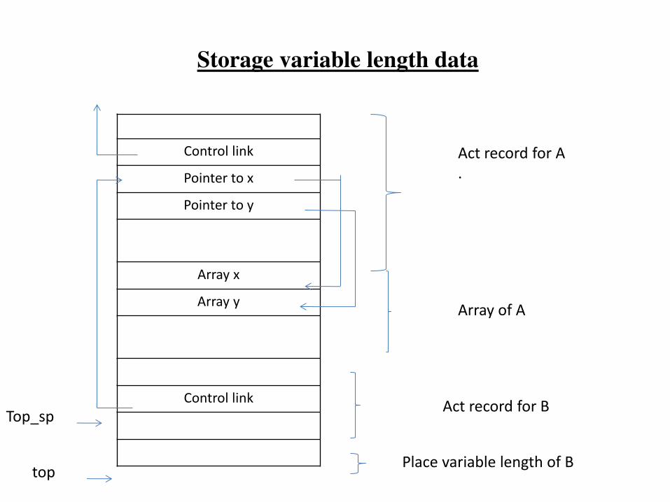
Storage variable length data

Control link

Pointer to x

Pointer to y

Array x

Array y

Control link

Act record for A

.

Array of A

Act record for B

Place variable length of B

Top_sp

top

Block structer and non block structure storage allocation

• The storage allocation can be done for 2 types of data variables

• 1. Local data

• 2. Non local data .

• Local data can be accessed with the help of activation record .

• Non local data can be accessed using scope information .

• The block structured storage allocation can be done using static

scope or lexical scope .

• The non block structured can be done by dynamic scope .

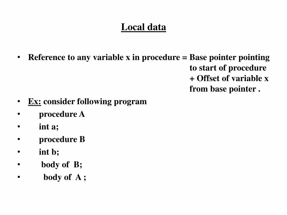
Local data

• Reference to any variable x in procedure = Base pointer pointing

to start of procedure

+ Offset of variable x

from base pointer .

• Ex: consider following program

• procedure A

• int a;

• procedure B

• int b;

• body of B;

• body of A ;

Local data

• The contents of stack along with base pointer and offset are as

shown below .

Return value

Dynamic link

Saved registers

parameters

Locals : a

Act rec for proc.

A

Base_ptr

offset

Access to local data

top

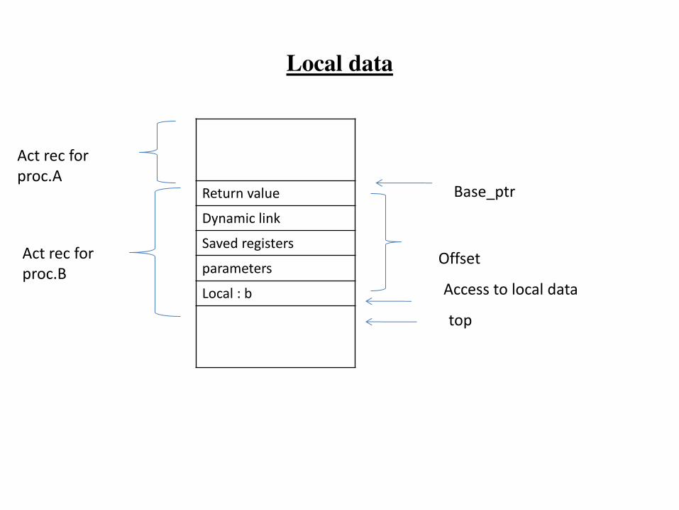
Local data

Return value

Dynamic link

Saved registers

parameters

Local : b

Base_ptr

Act rec for

proc.A

Act rec for

proc.B Offset

Access to local data

top

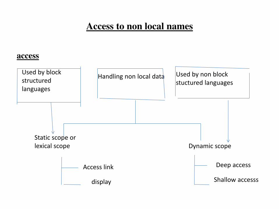
Access to non local names

access

Used by block

structured

languages

Handling non local data Used by non block

stuctured languages

Static scope or

lexical scope Dynamic scope

Access link

display

Deep access

Shallow accesss

Scope rules

Static scope rule : Is also called as lexical scope .

• In this type the scope is determined by examining the program

test . PASCAL,C and ADA are the languages that use the static

scope .

Dynamic scope : for non block structured languages this dynamic

scope allocation rules are used .

• Ex: LISP and SNOBOL

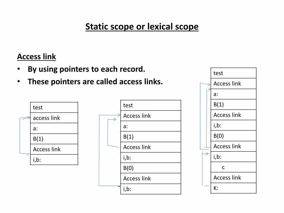
Static scope or lexical scope

Access link

• By using pointers to each record.

• These pointers are called access links.

test

access link

a:

B(1)

Access link

i,b:

test

Access link

a:

B(1)

Access link

i,b:

B(0)

Access link

i,b:

test

Access link

a:

B(1)

Access link

i,b:

B(0)

Access link

i,b:

c

Access link

K:

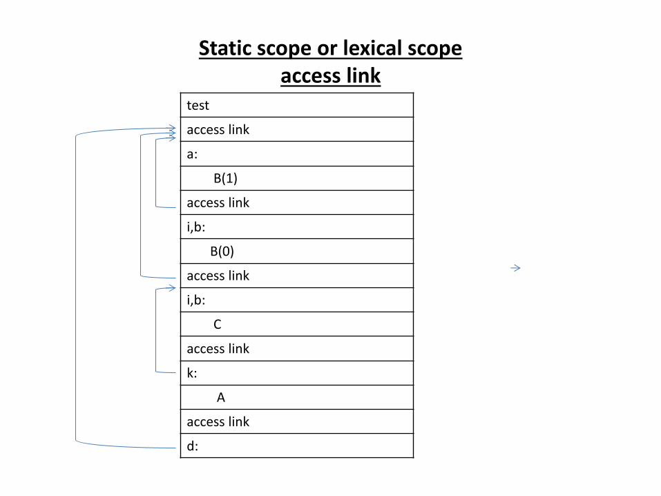
Static scope or lexical scope

access link

test

access link

a:

B(1)

access link

i,b:

B(0)

access link

i,b:

C

access link

k:

A

access link

d:

Static scope or lexical scope

• Displays :

• It is expensive to traverse down access link every time when a

particular local variable is accessed . To speed up the access to

non local can be achieved by maintaining an array of pointers

called display.

• In display

• An array of pointers to activation record is maintained.

• Array is indexing by nesting level.

• The pointers points to only accessible activation record.

• The display changes when a new activation occurs and it must be reset when control returns from the new activation.

Storage allocation for non block structured languages

• Dynamic scope :

• 1. deep access : the idea is keep a stack of active variables, use control links instead of access links and when you want to find a variable then search the stack from top to bottom looking for most recent activation record that contains the space for desired variables . This method of accessing non local variables is called Deep access .

• In this method a symbol table is needed to be used at run time .

• Shallow access : the idea is to keep a central storage with one slot for every variable name . If the names are not created at run time then that storage layout can be fixed at compile time otherwise when new activation of procedure occures,then that procedure changes the storage entries for its locals at entry and exit .

Comparison of Deep and Shallow access

• Deep access takes longer time to access the non locals

while Shallow access allows fast access .

• Shallow access has a overhead of handling procedure

entry and exit .

• Deep access needs a symbol table at run time .

UNIT-4

PART-A

Code Optimization

Introduction

• Concerns with machine-independent code optimization

90-10 rule: execution spends 90% time in 10% of the code.

It is moderately easy to achieve 90% optimization. The rest 10% is very difficult.

Identification of the 10% of the code is not possible for a compiler – it is the job of a profiler.

• In general, loops are the hot-spots

Introduction

• Criterion of code optimization

– Must preserve the semantic equivalence of the programs

– The algorithm should not be modified

– Transformation, on average should speed up the

execution of the program

– Worth the effort: Intellectual and compilation effort

spend on insignificant improvement.

Transformations are simple enough to have a good

effect

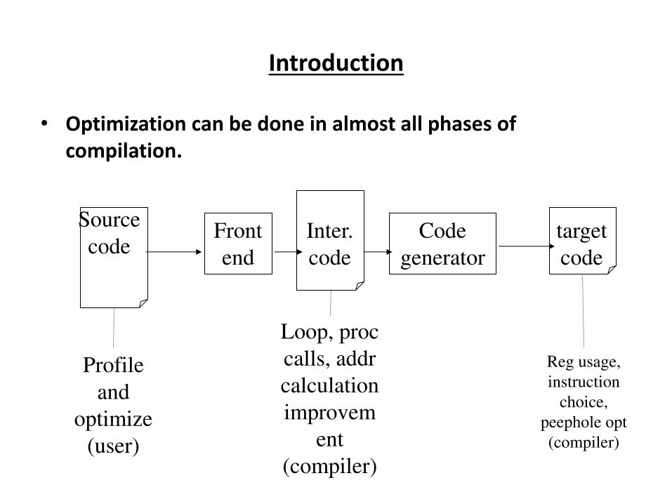
Introduction

• Optimization can be done in almost all phases of

compilation.

Front

end

Code

generator

Source

code Inter.

code

target

code

Profile

and

optimize

(user)

Loop, proc

calls, addr

calculation

improvem

ent

(compiler)

Reg usage,

instruction

choice,

peephole opt

(compiler)

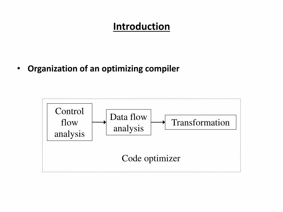
Introduction

• Organization of an optimizing compiler

Control

flow

analysis

Data flow

analysis Transformation

Code optimizer

Classifications of Optimization techniques

Peephole optimization

Local Optimization

Global Optimization

Inter-procedural

Intra-procedural

Loop Optimization

Factors influencing Optimization

• The target machine: machine dependent factors can be parameterized to compiler for fine tuning

• Architecture of Target CPU:

– Number of CPU registers

– RISC vs CISC

– Pipeline Architecture

– Number of functional units

• Machine Architecture

– Cache Size and type

– Cache/Memory transfer rate

Themes behind Optimization Techniques

• Avoid redundancy: something already computed need not be computed again

• Smaller code: less work for CPU, cache, and memory!

• Less jumps: jumps interfere with code pre-fetch

• Code locality: codes executed close together in time is generated close together in memory – increase locality of reference

• Extract more information about code: More info – better code generation

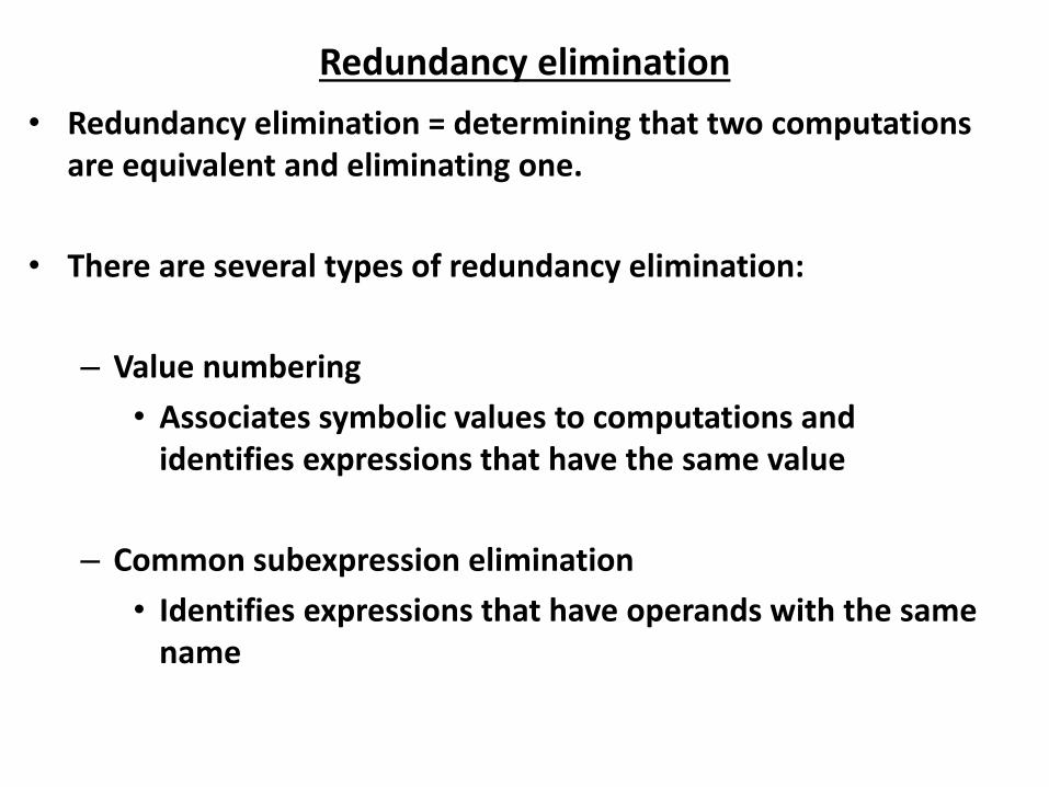
Redundancy elimination

• Redundancy elimination = determining that two computations

are equivalent and eliminating one.

• There are several types of redundancy elimination:

– Value numbering

• Associates symbolic values to computations and

identifies expressions that have the same value

– Common subexpression elimination

• Identifies expressions that have operands with the same

name

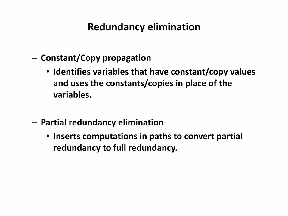
Redundancy elimination

– Constant/Copy propagation

• Identifies variables that have constant/copy values

and uses the constants/copies in place of the

variables.

– Partial redundancy elimination

• Inserts computations in paths to convert partial

redundancy to full redundancy.

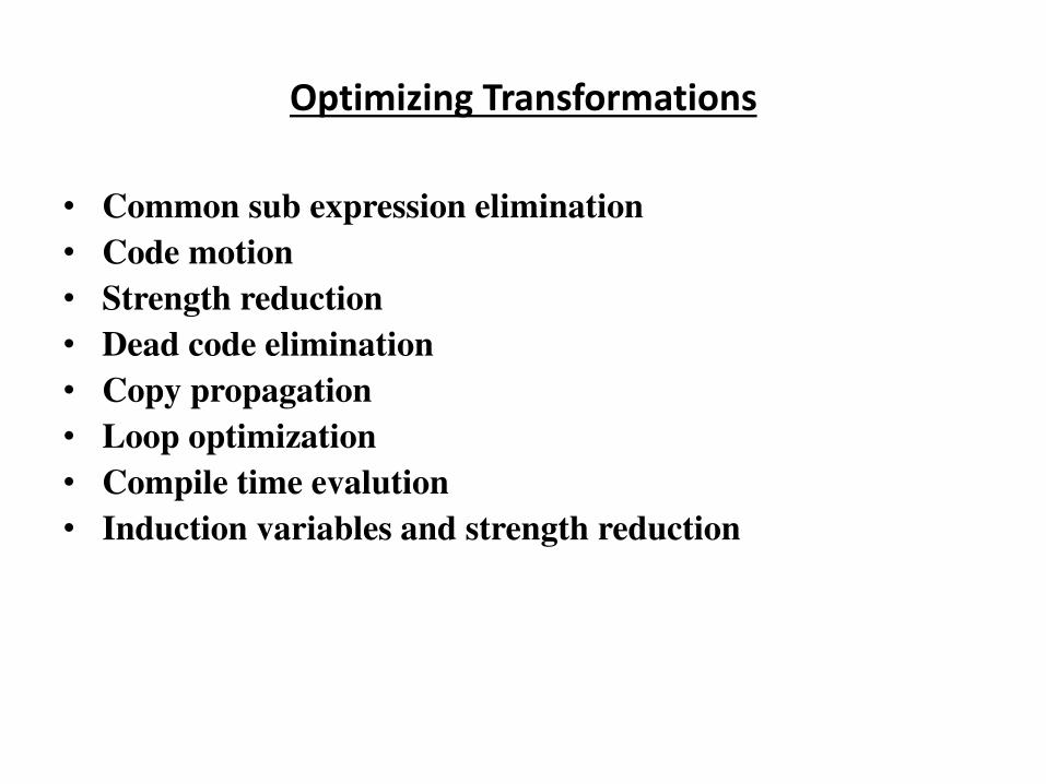
Optimizing Transformations

• Common sub expression elimination

• Code motion

• Strength reduction

• Dead code elimination

• Copy propagation

• Loop optimization

• Compile time evalution

• Induction variables and strength reduction

Compile-Time Evaluation

• Expressions whose values can be pre-computed at the

compilation time

• Two ways:

– Constant folding

– Constant propagation

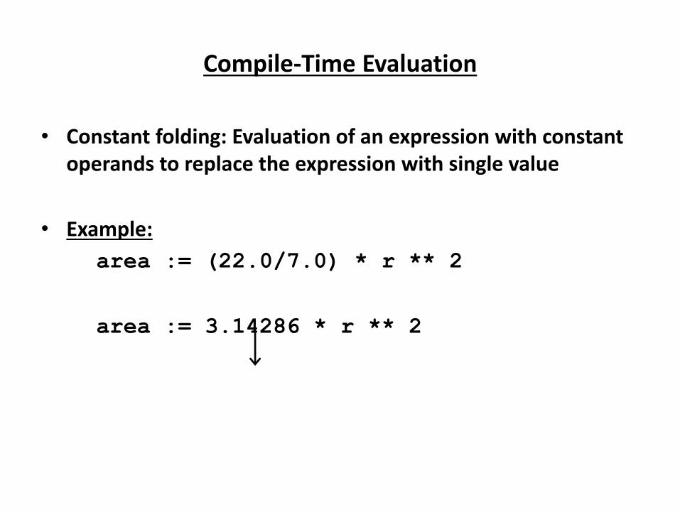
Compile-Time Evaluation

• Constant folding: Evaluation of an expression with constant

operands to replace the expression with single value

• Example:

area := (22.0/7.0) * r ** 2

area := 3.14286 * r ** 2

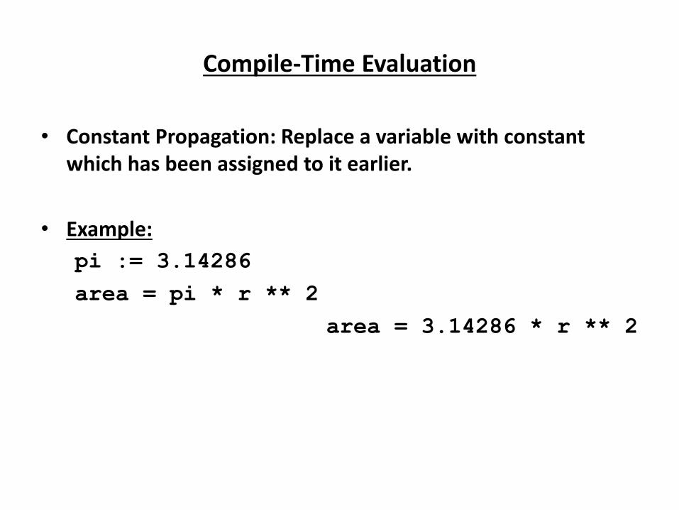
Compile-Time Evaluation

• Constant Propagation: Replace a variable with constant

which has been assigned to it earlier.

• Example:

pi := 3.14286

area = pi * r ** 2

area = 3.14286 * r ** 2

Constant Propagation

• What does it mean?

– Given an assignment x = c, where c is a constant, replace later uses of x with uses of c, provided there are no intervening assignments to x.

• Similar to copy propagation

• Extra feature: It can analyze constant-value conditionals to determine whether a branch should be executed or not.

• When is it performed?

– Early in the optimization process.

• What is the result?

– Smaller code

– Fewer registers

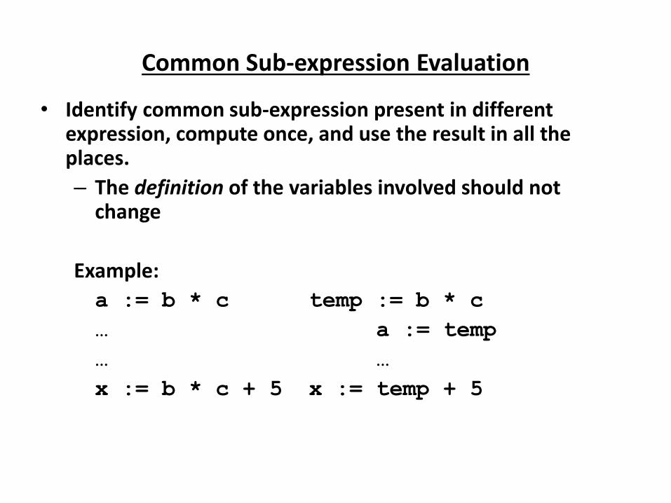
Common Sub-expression Evaluation

• Identify common sub-expression present in different expression, compute once, and use the result in all the places.

– The definition of the variables involved should not change

Example:

a := b * c temp := b * c

… a := temp

… … x := b * c + 5 x := temp + 5

Common Subexpression Elimination

• Local common subexpression elimination

– Performed within basic blocks

– Algorithm sketch:

• Traverse BB from top to bottom

• Maintain table of expressions evaluated so far

– if any operand of the expression is redefined,

remove it from the table

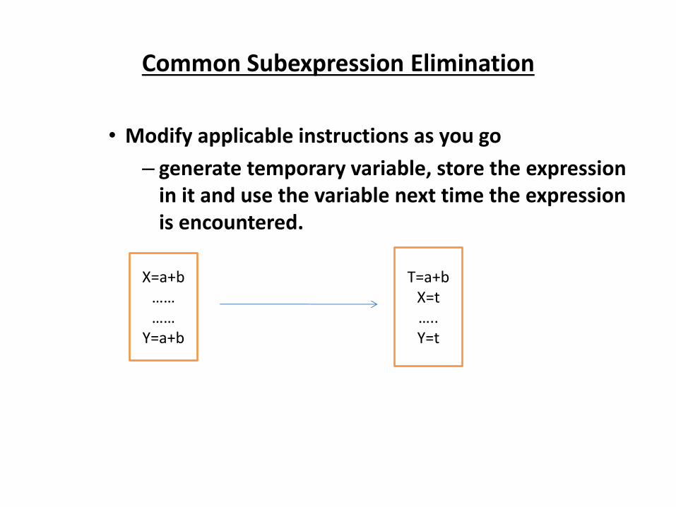
Common Subexpression Elimination

• Modify applicable instructions as you go

– generate temporary variable, store the expression

in it and use the variable next time the expression

is encountered.

X=a+b

……

……

Y=a+b

T=a+b

X=t

….. Y=t

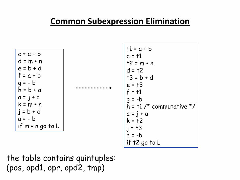
Common Subexpression Elimination

c = a + b d = m * n e = b + d f = a + b g = - b h = b + a a = j + a k = m * n j = b + d a = - b if m * n go to L

t1 = a + b c = t1 t2 = m * n d = t2 t3 = b + d e = t3 f = t1 g = -b h = t1 /* commutative */ a = j + a k = t2 j = t3 a = -b if t2 go to L

the table contains quintuples: (pos, opd1, opr, opd2, tmp)

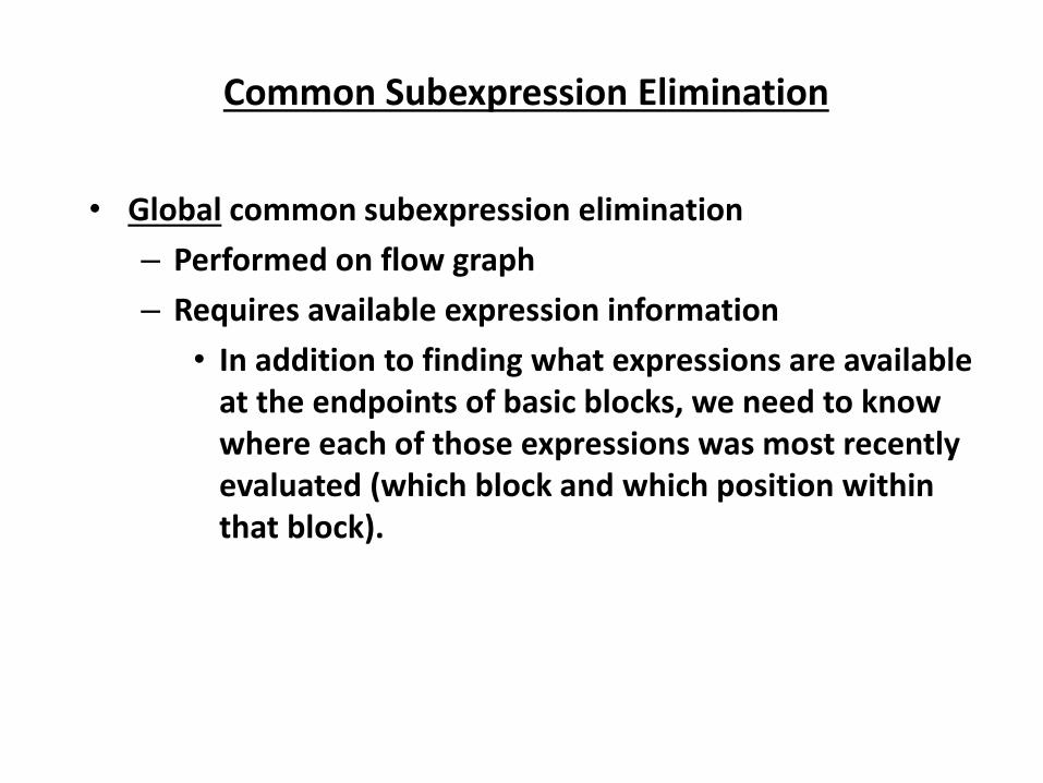
Common Subexpression Elimination

• Global common subexpression elimination

– Performed on flow graph

– Requires available expression information

• In addition to finding what expressions are available

at the endpoints of basic blocks, we need to know

where each of those expressions was most recently

evaluated (which block and which position within

that block).

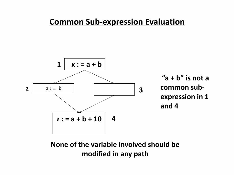
Common Sub-expression Evaluation

z : = a + b + 10

a : = b

1

2 3

4

a + is ot a common sub-

expression in 1

and 4

None of the variable involved should be

modified in any path

x : = a + b

Code Motion

• Moving code from one part of the program to other without

modifying the algorithm

– Reduce size of the program

– Reduce execution frequency of the code subjected to

movement

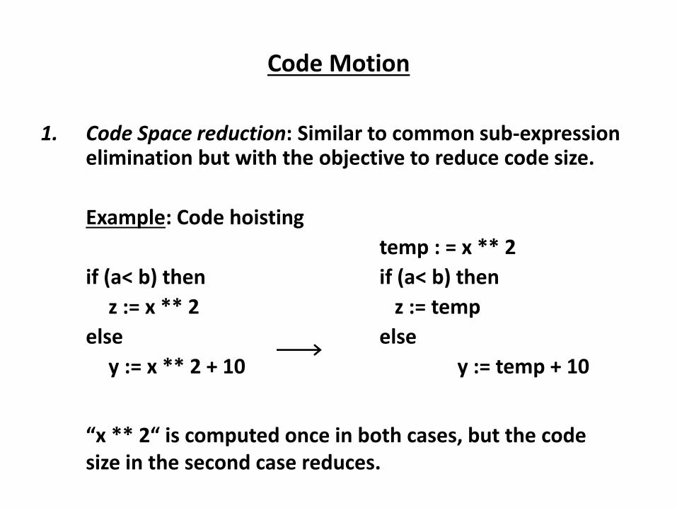
Code Motion

1. Code Space reduction: Similar to common sub-expression elimination but with the objective to reduce code size.

Example: Code hoisting

temp : = x ** 2

if (a< b) then if (a< b) then

z := x ** 2 z := temp

else else

y := x ** 2 + 10 y := temp + 10

** is o puted o e i oth ases, ut the ode size in the second case reduces.

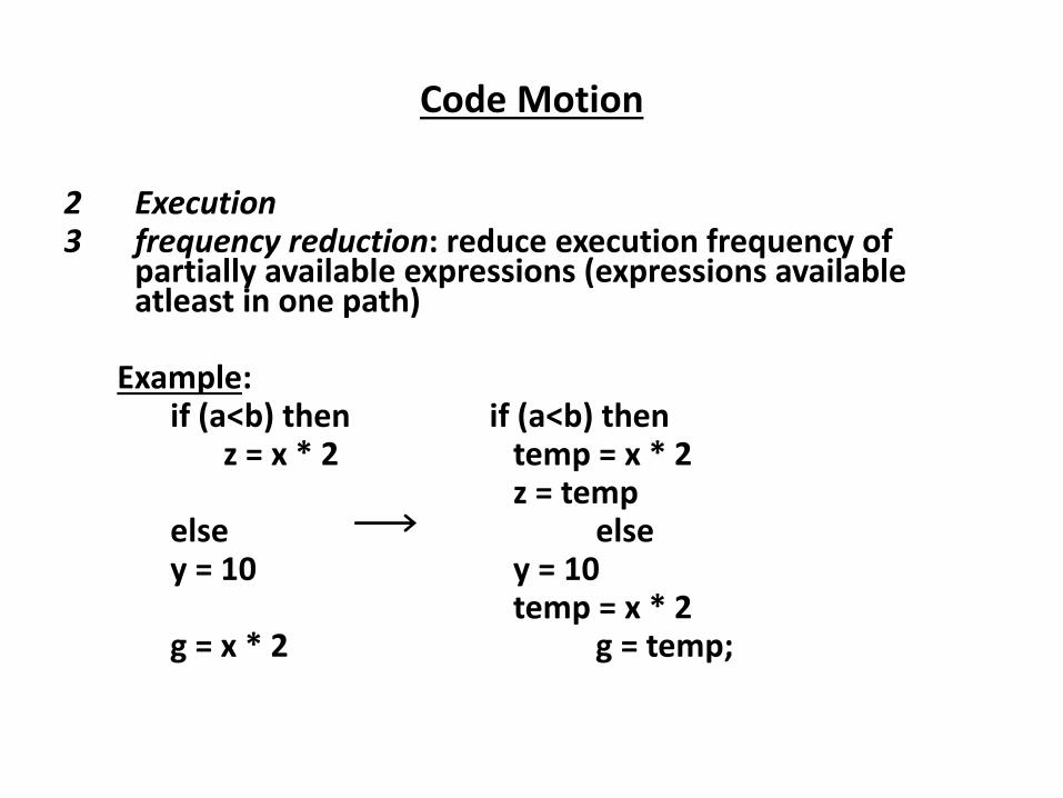
Code Motion

2 Execution 3 frequency reduction: reduce execution frequency of

partially available expressions (expressions available atleast in one path)

Example:

if (a<b) then if (a<b) then z = x * 2 temp = x * 2 z = temp else else y = 10 y = 10 temp = x * 2 g = x * 2 g = temp;

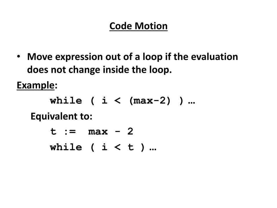
Code Motion

• Move expression out of a loop if the evaluation

does not change inside the loop.

Example:

while ( i < (max-2) ) … Equivalent to:

t := max - 2

while ( i < t ) …

Code Motion

• Safety of Code movement

Movement of an expression e from a basic block bi to another block bj, is safe if it does not introduce any new occurrence of e along any path.

Example: Unsafe code movement

temp = x * 2

if (a<b) then if (a<b) then

z = x * 2 z = temp

else else

y = 10 y = 10

Strength Reduction

• Replacement of an operator with a less costly one.

Example:

temp = 5;

for i=1 to 10 do for i=1 to 10 do

… …

x = i * 5 x = temp

… …

temp = temp + 5

end end

• Typical cases of strength reduction occurs in address calculation of array references.

• Applies to integer expressions involving induction variables (loop optimization)

Dead Code Elimination

• Dead Code are portion of the program which will not be executed in any path of the program.

– Can be removed

• Examples:

– No control flows into a basic block

– A variable is dead at a point -> its value is not used anywhere in the program

– An assignment is dead -> assignment assigns a value to a dead variable

Dead Code Elimination

• Examples:

•i=j;

•…

•X=i+10

•The optimization can be performed by

•Eliminating the assignment statement

•i=j

.

This assignment statement is called dead

assignment .

Copy Propagation

• What does it mean?

– Given an assignment x = y, replace later uses of x with

uses of y, provided there are no intervening assignments

to x or y.

• When is it performed?

– At any level, but usually early in the optimization

process.

• What is the result?

– Smaller code

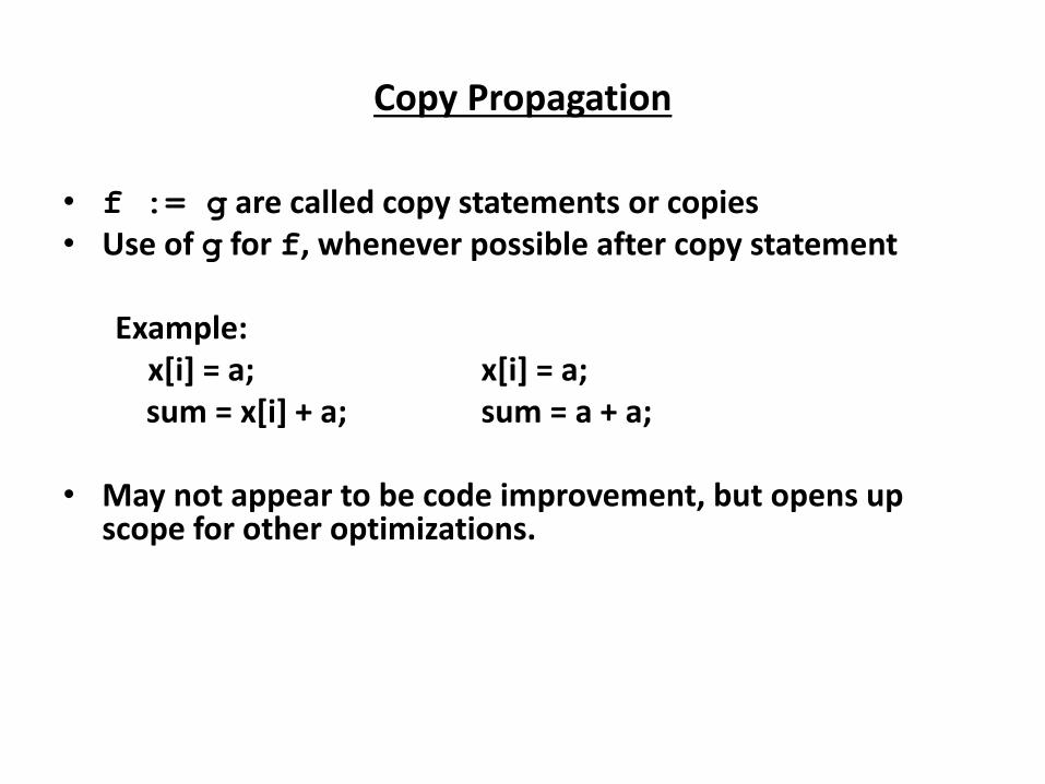
Copy Propagation

• f := g are called copy statements or copies

• Use of g for f, whenever possible after copy statement

Example:

x[i] = a; x[i] = a;

sum = x[i] + a; sum = a + a;

• May not appear to be code improvement, but opens up scope for other optimizations.

Local Copy Propagation

• Local copy propagation

– Performed within basic blocks

– Algorithm sketch:

• traverse BB from top to bottom

• maintain table of copies encountered so far

• modify applicable instructions as you go

Loop Optimization

• Decrease the number if instruction in the inner loop

• Even if we increase no of instructions in the outer loop

• Techniques:

– Code motion

– Induction variable elimination

– Strength reduction

Peephole Optimization

• Pass over generated code to examine a few instructions,

typically 2 to 4

– Redundant instruction Elimination: Use algebraic

identities

– Flow of control optimization: removal of redundant

jumps

– Use of machine idioms

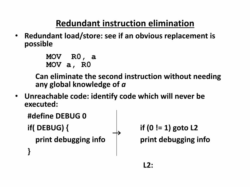
Redundant instruction elimination

• Redundant load/store: see if an obvious replacement is possible

MOV R0, a MOV a, R0

Can eliminate the second instruction without needing any global knowledge of a

• Unreachable code: identify code which will never be executed:

#define DEBUG 0

if( DEBUG) { if (0 != 1) goto L2

print debugging info print debugging info

}

L2:

Algebraic identities

• Worth recognizing single instructions with a constant operand:

A * 1 = A

A * 0 = 0

A / 1 = A

A * 2 = A + A

More delicate with floating-point

• Strength reduction:

A ^ 2 = A * A

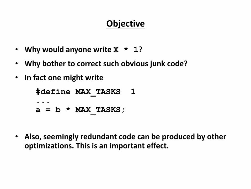
Objective

• Why would anyone write X * 1?

• Why bother to correct such obvious junk code?

• In fact one might write

#define MAX_TASKS 1 ... a = b * MAX_TASKS;

• Also, seemingly redundant code can be produced by other optimizations. This is an important effect.

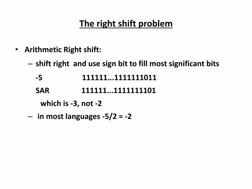
The right shift problem

• Arithmetic Right shift:

– shift right and use sign bit to fill most significant bits

-5 111111...1111111011

SAR 111111...1111111101

which is -3, not -2

– in most languages -5/2 = -2

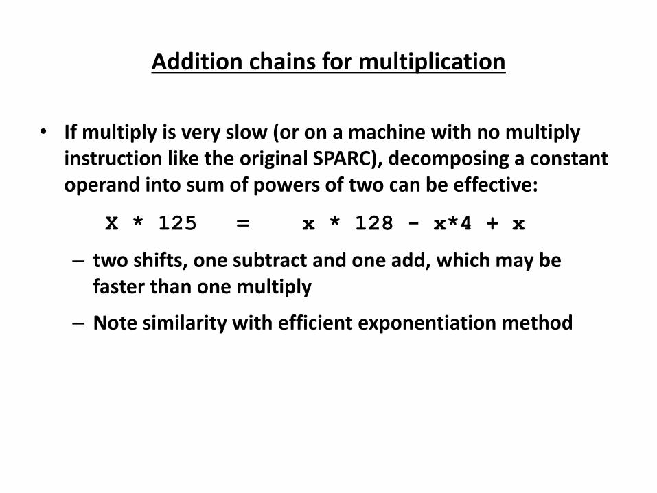
Addition chains for multiplication

• If multiply is very slow (or on a machine with no multiply

instruction like the original SPARC), decomposing a constant

operand into sum of powers of two can be effective:

X * 125 = x * 128 - x*4 + x

– two shifts, one subtract and one add, which may be

faster than one multiply

– Note similarity with efficient exponentiation method

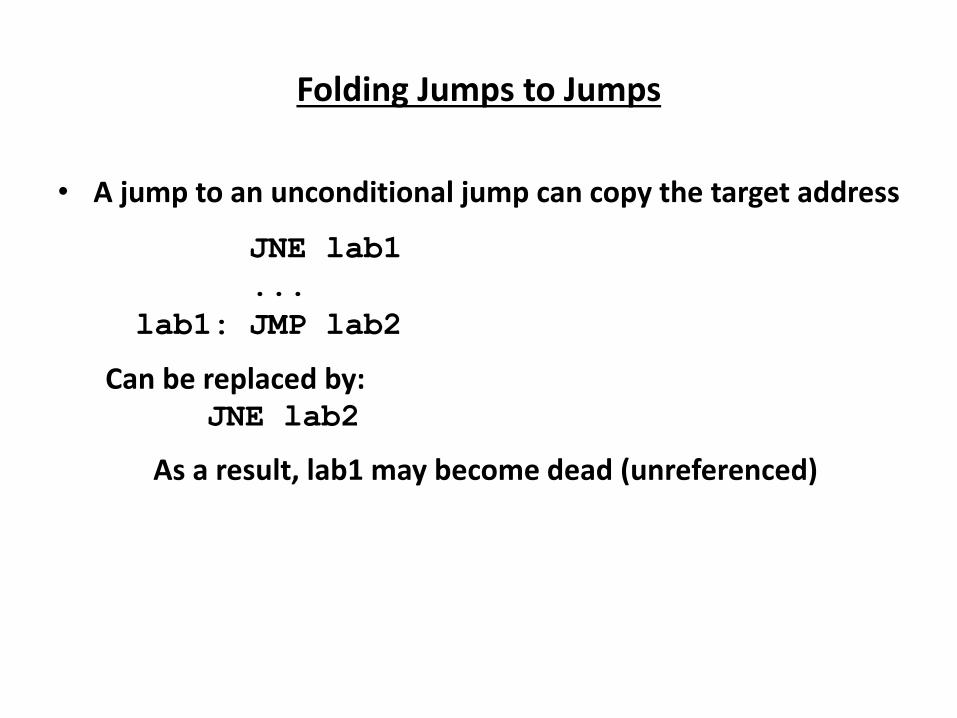
Folding Jumps to Jumps

• A jump to an unconditional jump can copy the target address

JNE lab1 ... lab1: JMP lab2

Can be replaced by:

JNE lab2

As a result, lab1 may become dead (unreferenced)

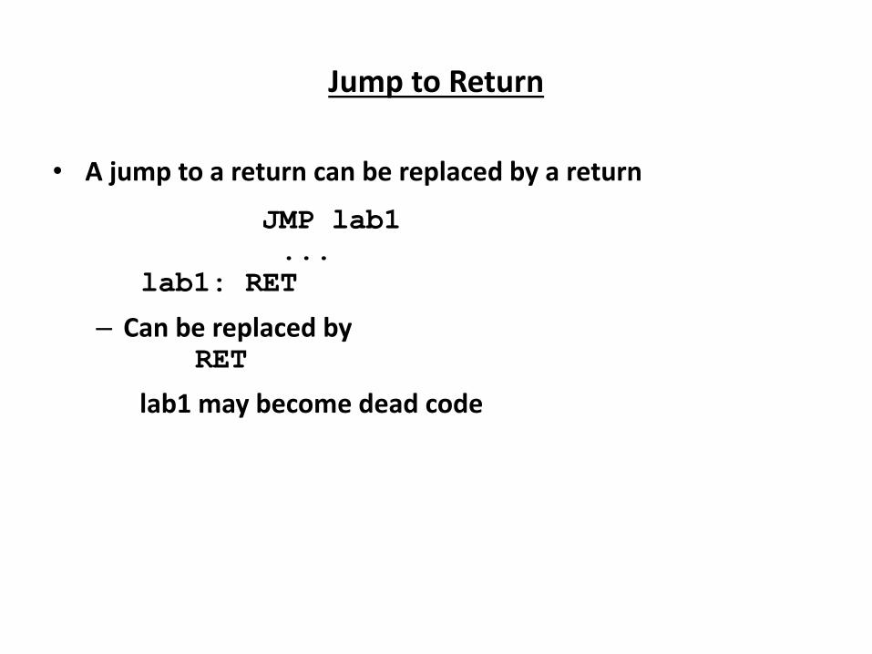
Jump to Return

• A jump to a return can be replaced by a return

JMP lab1 ... lab1: RET

– Can be replaced by RET

lab1 may become dead code

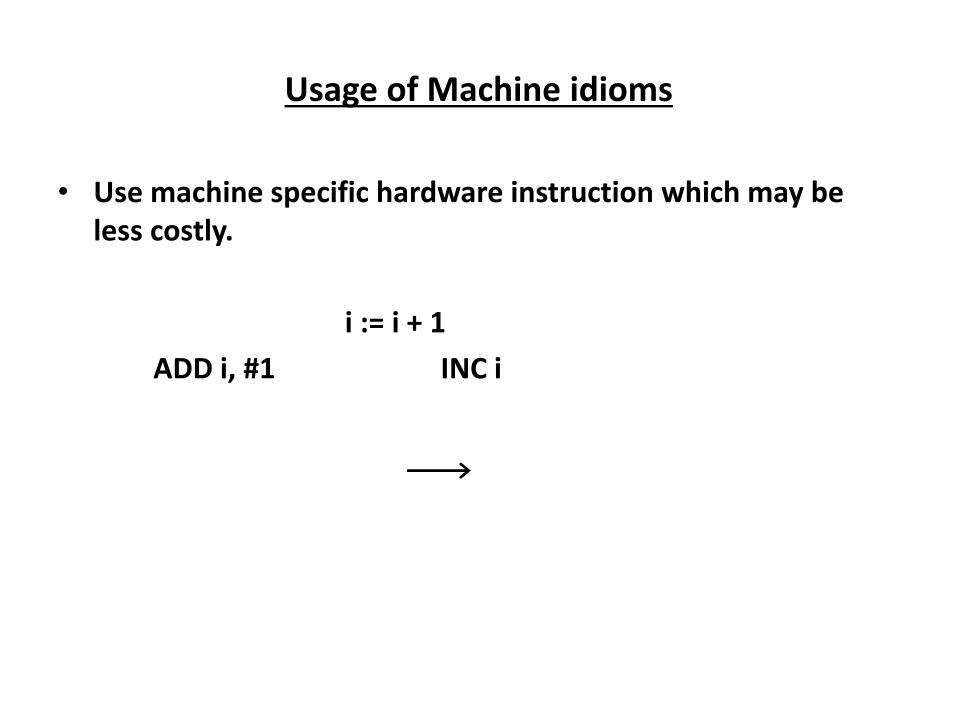
Usage of Machine idioms

• Use machine specific hardware instruction which may be

less costly.

i := i + 1

ADD i, #1 INC i

Local Optimization

Optimization of Basic Blocks

• Many structure preserving transformations can be

implemented by construction of DAGs of basic blocks

DAG representation

of Basic Block (BB)

• Leaves are labeled with unique identifier (var name or const)

• Interior nodes are labeled by an operator symbol

• Nodes optionally have a list of labels (identifiers)

• Edges relates operands to the operator (interior nodes are

operator)

• Interior node represents computed value

– Identifier in the label are deemed to hold the value

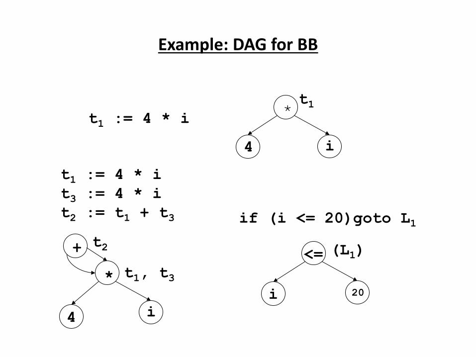
Example: DAG for BB

t1 := 4 * i t1

*

i 4

t1 := 4 * i t3 := 4 * i t2 := t1 + t3

*

i 4

+

t1, t3

t2

if (i <= 20)goto L1

<=

i 20

(L1)

Construction of DAGs for BB

• I/p: Basic block, B

• O/p: A DAG for B containing the following information:

1) A label for each node

2) For leaves the labels are ids or consts

3) For interior nodes the labels are operators

4) For each node a list of attached ids (possible empty list, no consts)

Construction of DAGs for BB

• Data structure and functions:

– Node:

1) Label: label of the node

2) Left: pointer to the left child node

3) Right: pointer to the right child node

4) List: list of additional labels (empty for leaves)

– Node (id): returns the most recent node created for id. Else return undef

– Create(id,l,r): create a node with label id with l as left child and r as right child. l and r are optional params.

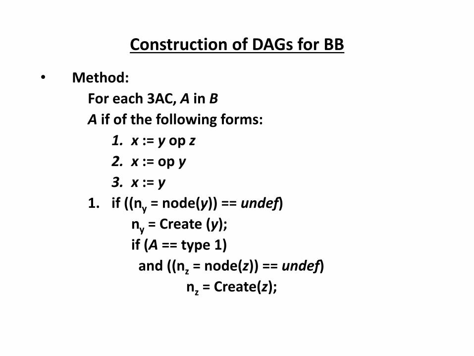
Construction of DAGs for BB

• Method:

For each 3AC, A in B

A if of the following forms:

1. x := y op z

2. x := op y

3. x := y

1. if ((ny = node(y)) == undef)

ny = Create (y);

if (A == type 1)

and ((nz = node(z)) == undef)

nz = Create(z);

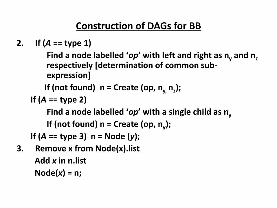
Construction of DAGs for BB

2. If (A == type 1)

Fi d a ode la elled op ith left a d ight as y and nz respectively [determination of common sub-expression]

If (not found) n = Create (op, ny, nz);

If (A == type 2)

Fi d a ode la elled op ith a si gle hild as y

If (not found) n = Create (op, ny);

If (A == type 3) n = Node (y);

3. Remove x from Node(x).list

Add x in n.list

Node(x) = n;

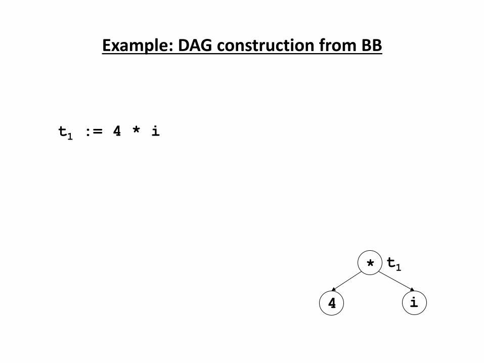
Example: DAG construction from BB

t1 := 4 * i

*

i 4

t1

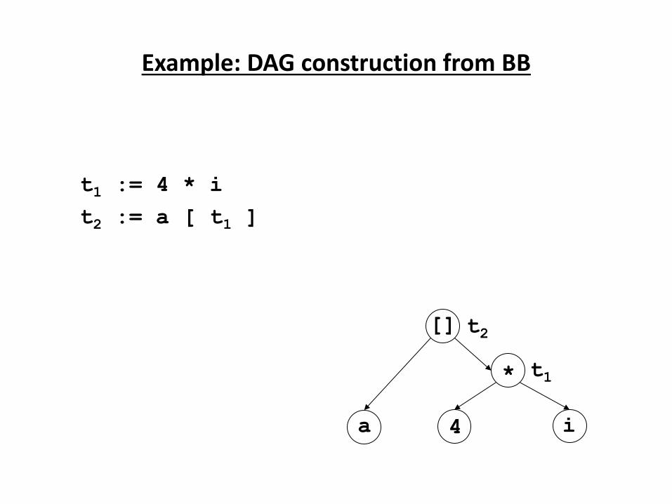
Example: DAG construction from BB

t1 := 4 * i

t2 := a [ t1 ]

*

i 4

t1

[]

a

t2

Example: DAG construction from BB

t1 := 4 * i

t2 := a [ t1]

t3 := 4 * i

*

i 4

t1, t3

[]

a

t2

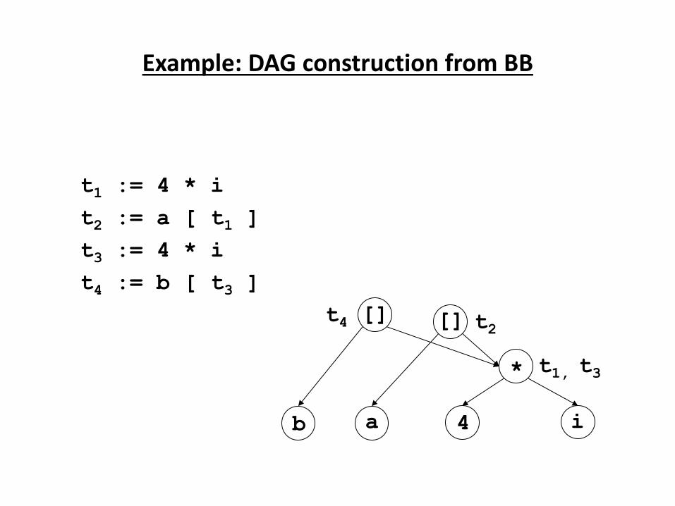
Example: DAG construction from BB

t1 := 4 * i

t2 := a [ t1 ]

t3 := 4 * i

t4 := b [ t3 ]

*

i 4

t1, t3

[]

a

t2 []

b

t4

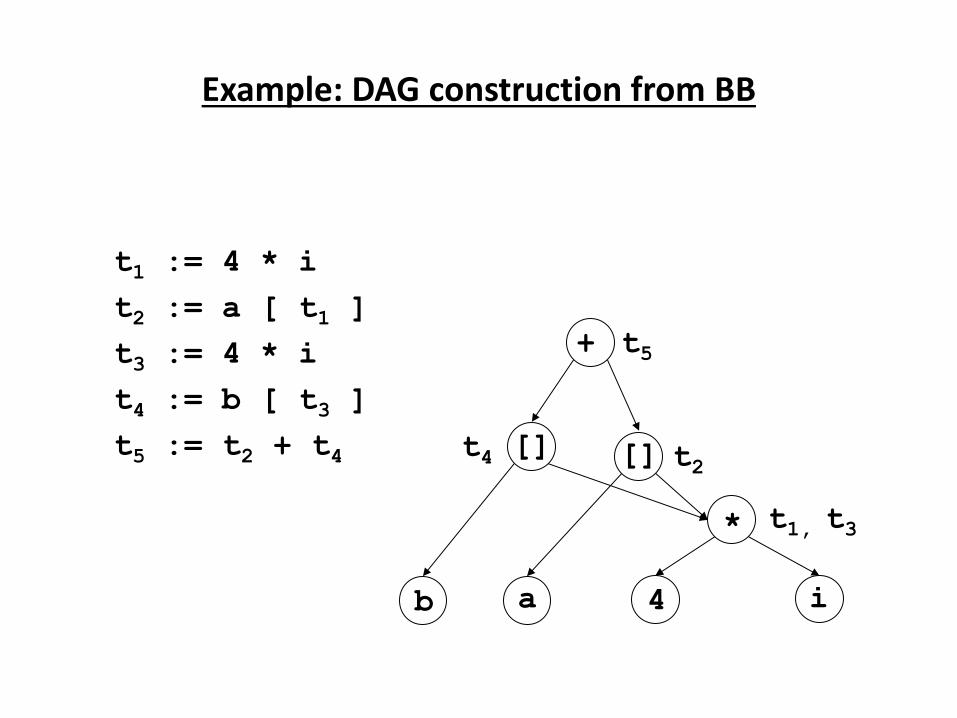
Example: DAG construction from BB

t1 := 4 * i

t2 := a [ t1 ]

t3 := 4 * i

t4 := b [ t3 ]

t5 := t2 + t4

*

i 4

t1, t3

[]

a

t2 []

b

t4

t5 +

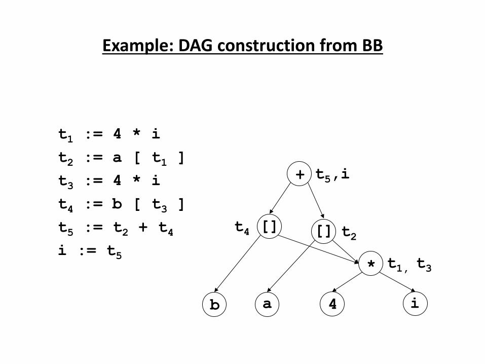
Example: DAG construction from BB

t1 := 4 * i

t2 := a [ t1 ]

t3 := 4 * i

t4 := b [ t3 ]

t5 := t2 + t4 i := t5

*

i 4

t1, t3

[]

a

t2 []

b

t4

t5,i +

DAG of a Basic Block

• Observations:

– A leaf node for the initial value of an id

– A node n for each statement s

– The children of node n are the last definition (prior to s)

of the operands of n

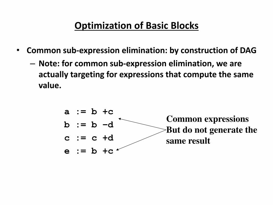
Optimization of Basic Blocks

• Common sub-expression elimination: by construction of DAG

– Note: for common sub-expression elimination, we are

actually targeting for expressions that compute the same

value.

a := b +c

b := b –d c := c +d

e := b +c

Common expressions

But do not generate the

same result

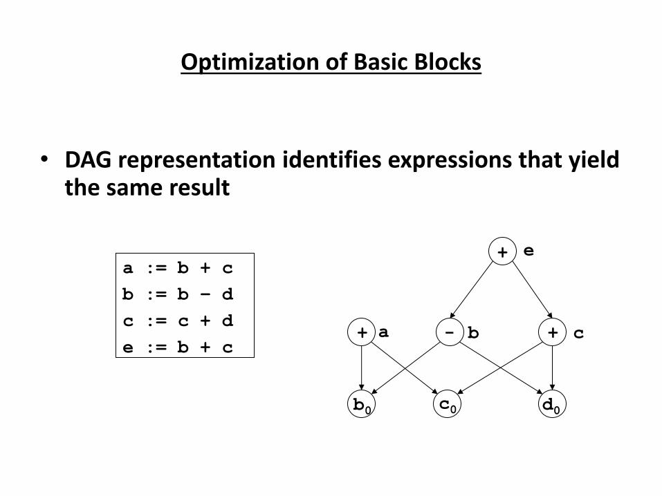
Optimization of Basic Blocks

• DAG representation identifies expressions that yield the same result

a := b + c

b := b – d c := c + d

e := b + c

b0 c0 d0

+

+ + - a b c

e

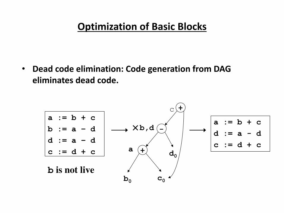
Optimization of Basic Blocks

• Dead code elimination: Code generation from DAG

eliminates dead code.

a := b + c

b := a – d d := a – d c := d + c

b is not live

c

a := b + c

d := a - d

c := d + c

b0 c0

d0 +

-

+

a

b,d ×

Loop Optimization

Loop Optimizations

• Most important set of optimizations

– Programs are likely to spend more time in loops

• Presumption: Loop has been identified

• Optimizations:

– Loop invariant code removal

– Induction variable strength reduction

– Induction variable reduction

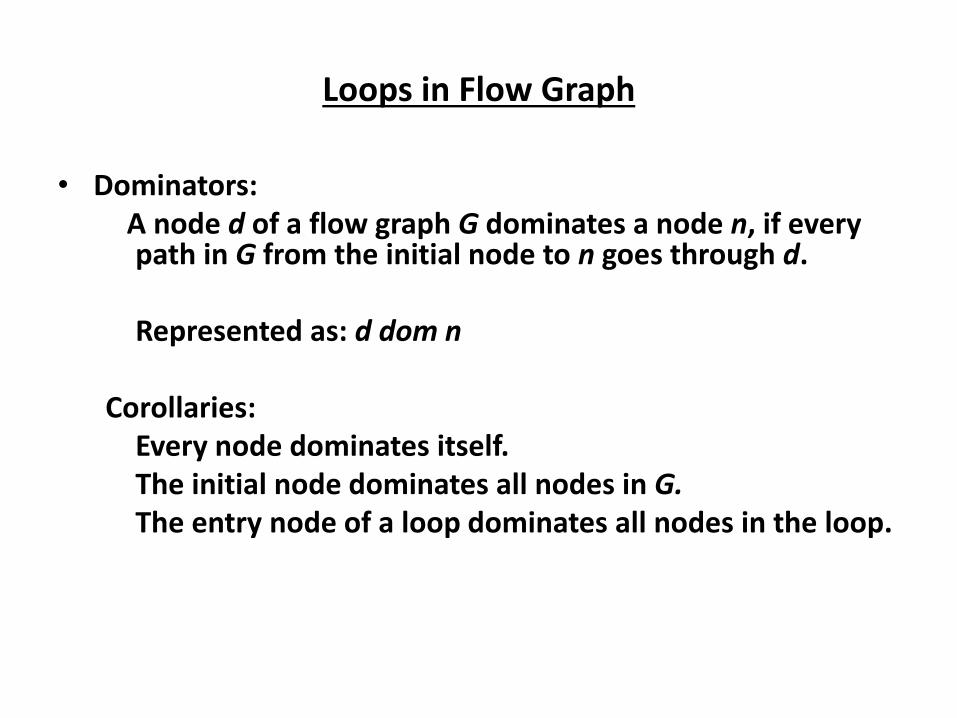
Loops in Flow Graph

• Dominators:

A node d of a flow graph G dominates a node n, if every path in G from the initial node to n goes through d.

Represented as: d dom n

Corollaries:

Every node dominates itself.

The initial node dominates all nodes in G.

The entry node of a loop dominates all nodes in the loop.

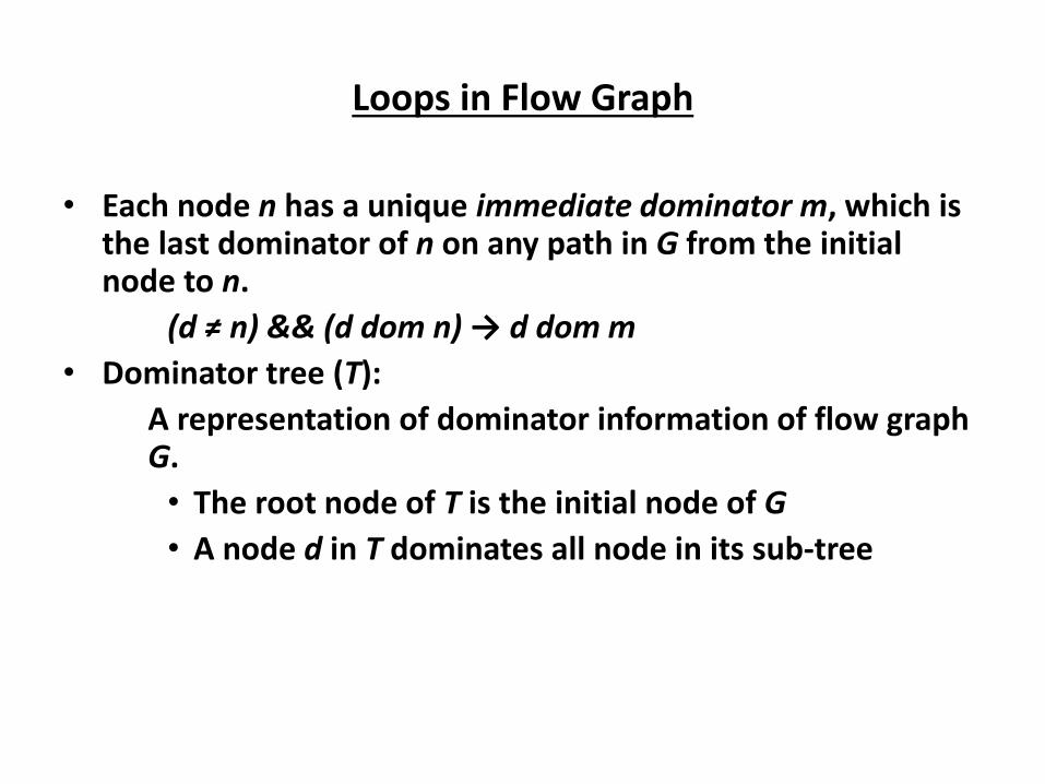
Loops in Flow Graph

• Each node n has a unique immediate dominator m, which is the last dominator of n on any path in G from the initial node to n.

(d ≠ n) && (d dom n) → d dom m

• Dominator tree (T):

A representation of dominator information of flow graph G.

• The root node of T is the initial node of G

• A node d in T dominates all node in its sub-tree

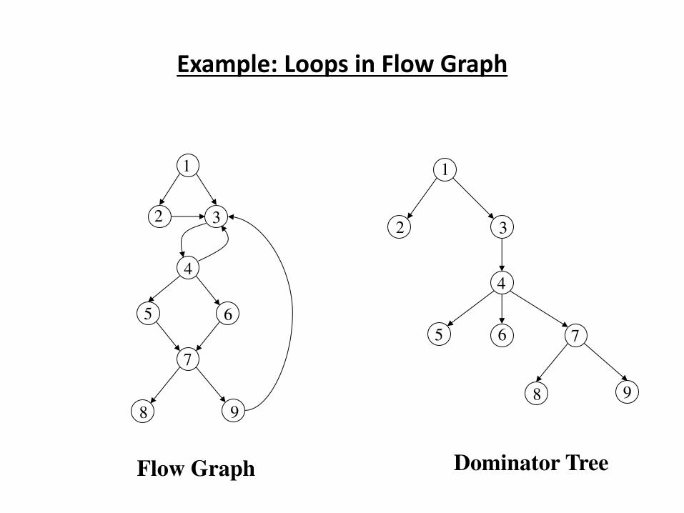
Example: Loops in Flow Graph

1

2 3

4

5 6 7

8 9

Flow Graph Dominator Tree

1

2 3

4

5 6

7

8 9

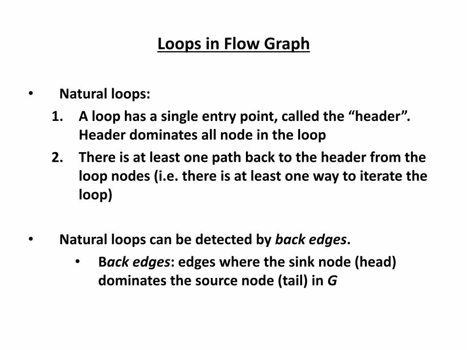
Loops in Flow Graph

• Natural loops:

1. A loop has a si gle e t poi t, alled the heade . Header dominates all node in the loop

2. There is at least one path back to the header from the

loop nodes (i.e. there is at least one way to iterate the

loop)

• Natural loops can be detected by back edges.

• Back edges: edges where the sink node (head)

dominates the source node (tail) in G

Loop Optimization

• Loop interchange: exchange inner loops with outer loops

• Loop splitting: attempts to simplify a loop or eliminate dependencies by breaking it into multiple loops which have the same bodies but iterate over different contiguous portions of the index range.

– A useful special case is loop peeling - simplify a loop with a problematic first iteration by performing that iteration separately before entering the loop.

Loop Optimization

• Loop fusion: two adjacent loops would iterate the same number of times, their bodies can be combined as long as they make no reference to each other's data

• Loop fission: break a loop into multiple loops over the same index range but each taking only a part of the loop's body.

• Loop unrolling: duplicates the body of the loop multiple times

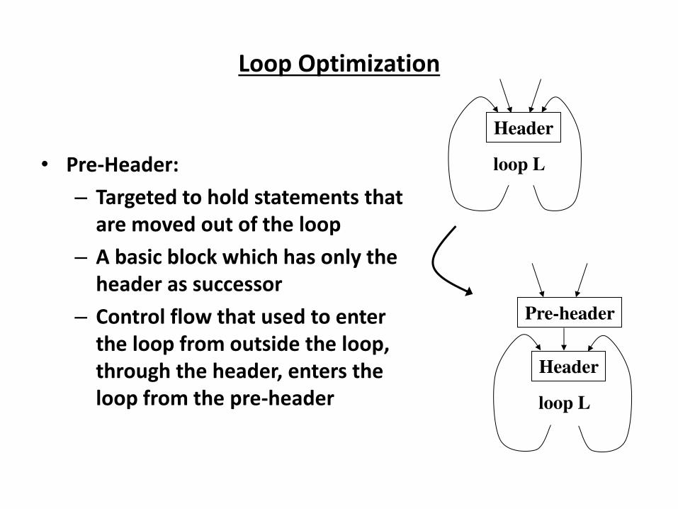
Loop Optimization

• Pre-Header:

– Targeted to hold statements that

are moved out of the loop

– A basic block which has only the

header as successor

– Control flow that used to enter

the loop from outside the loop,

through the header, enters the

loop from the pre-header

Header

loop L

Header

loop L

Pre-header

Loop Invariant Code Removal

• Move out to pre-header the statements whose source

operands do not change within the loop.

– Be careful with the memory operations

– Be careful with statements which are executed in some of

the iterations

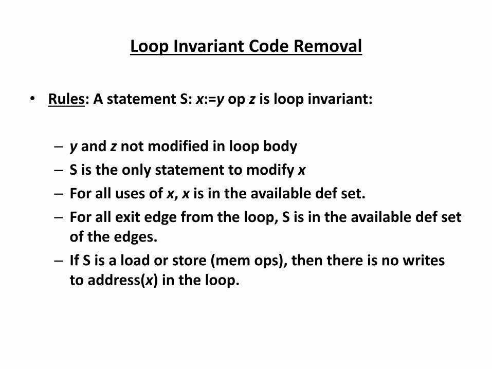
Loop Invariant Code Removal

• Rules: A statement S: x:=y op z is loop invariant:

– y and z not modified in loop body

– S is the only statement to modify x

– For all uses of x, x is in the available def set.

– For all exit edge from the loop, S is in the available def set

of the edges.

– If S is a load or store (mem ops), then there is no writes

to address(x) in the loop.

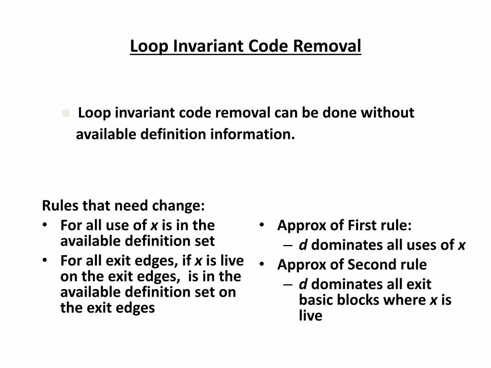
Loop Invariant Code Removal

Rules that need change:

• For all use of x is in the available definition set

• For all exit edges, if x is live on the exit edges, is in the available definition set on the exit edges

• Approx of First rule:

– d dominates all uses of x

• Approx of Second rule

– d dominates all exit basic blocks where x is live

Loop invariant code removal can be done without

available definition information.

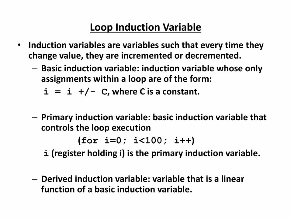
Loop Induction Variable

• Induction variables are variables such that every time they change value, they are incremented or decremented.

– Basic induction variable: induction variable whose only assignments within a loop are of the form:

i = i +/- C, where C is a constant.

– Primary induction variable: basic induction variable that controls the loop execution

(for i=0; i<100; i++)

i (register holding i) is the primary induction variable.

– Derived induction variable: variable that is a linear function of a basic induction variable.

Loop Induction Variable

• Basic: r4, r7, r1

• Primary: r1

• Derived: r2

r2 = r1 * 4

r4 = r7 + 3

r7 = r7 + 1

r10 = *r2

r3 = *r4

r9 = r1 * r3

r10 = r9 >> 4

*r2 = r10

r1 = r1 + 4

If(r1 < 100) goto Loop

Loop:

r1 = 0

r7 = &A

Induction Variable Strength Reduction

• Create basic induction variables from derived induction variables.

• Rules: (S: x := y op z)

– op is *, <<, +, or –

– y is a induction variable

– z is invariant

– No other statement modifies x

– x is not y or z

– x is a register

Induction Variable Strength Reduction

• Transformation:

Insert the following into the bottom of pre-header:

new_reg = expression of target statement S

if (opcode(S)) is not add/sub, insert to the bottom of the preheader

new_inc = inc(y,op,z)

else

new_inc = inc(x)

Insert the following at each update of y

new_reg = new_reg + new_inc

Change S: x = new_reg

Function: inc()

Calculate the amount of inc

for 1st param.

Example: Induction Variable Strength Reduction

r5 = r4 - 3

r4 = r4 + 1

r7 = r4 *r9

r6 = r4 << 2

new_reg = r4 * r9

new_inc = r9

r5 = r4 - 3

r4 = r4 + 1

new_reg += new_inc

r7 = new_reg

r6 = r4 << 2

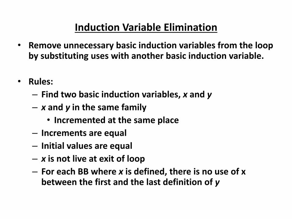
Induction Variable Elimination

• Remove unnecessary basic induction variables from the loop by substituting uses with another basic induction variable.

• Rules:

– Find two basic induction variables, x and y

– x and y in the same family

• Incremented at the same place

– Increments are equal

– Initial values are equal

– x is not live at exit of loop

– For each BB where x is defined, there is no use of x between the first and the last definition of y

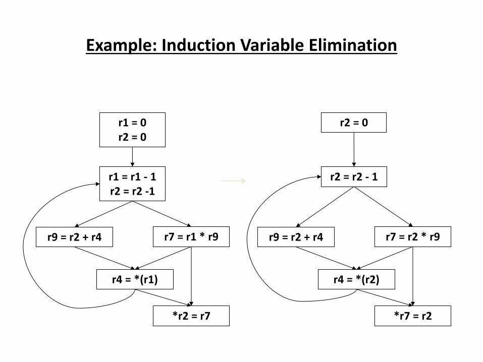
Example: Induction Variable Elimination

r1 = 0

r2 = 0

r1 = r1 - 1

r2 = r2 -1

r9 = r2 + r4 r7 = r1 * r9

r4 = *(r1)

*r2 = r7

r2 = 0

r2 = r2 - 1

r9 = r2 + r4 r7 = r2 * r9

r4 = *(r2)

*r7 = r2

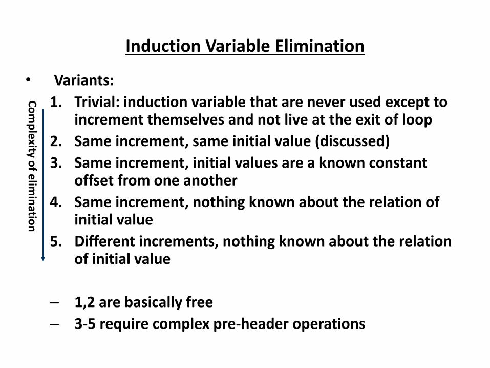
Induction Variable Elimination

• Variants:

1. Trivial: induction variable that are never used except to increment themselves and not live at the exit of loop

2. Same increment, same initial value (discussed)

3. Same increment, initial values are a known constant offset from one another

4. Same increment, nothing known about the relation of initial value

5. Different increments, nothing known about the relation of initial value

– 1,2 are basically free

– 3-5 require complex pre-header operations

Co

mp

lexity

of e

limin

atio

n

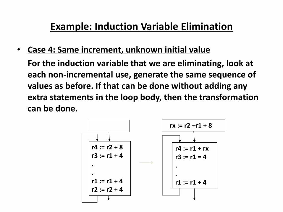
Example: Induction Variable Elimination

• Case 4: Same increment, unknown initial value

For the induction variable that we are eliminating, look at

each non-incremental use, generate the same sequence of

values as before. If that can be done without adding any

extra statements in the loop body, then the transformation

can be done.

r4 := r2 + 8

r3 := r1 + 4

.

.

r1 := r1 + 4

r2 := r2 + 4

rx := r2 –r1 + 8

r4 := r1 + rx

r3 := r1 = 4

.

.

r1 := r1 + 4

Loop Unrolling

• Replicate the body of a loop (N-1) times, resulting in total N

copies.

– Enable overlap of operations from different iterations

– Increase potential of instruction level parallelism (ILP)

• Variants:

– Unroll multiple of known trip counts

– Unroll with remainder loop

– While loop unroll

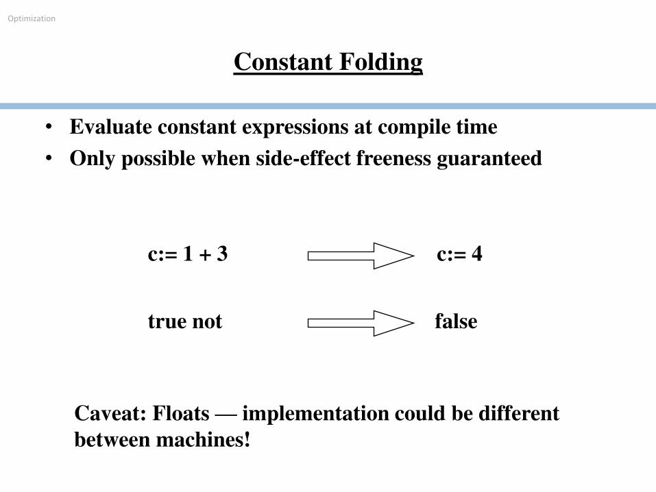
Optimization

Constant Folding

• Evaluate constant expressions at compile time

• Only possible when side-effect freeness guaranteed

c:= 1 + 3 c:= 4

true not false

Caveat: Floats — implementation could be different

between machines!

Unit-4

PART-B

DATA FLOW ANALYSIS

553

Global Data Flow Analysis

• Collect information about the whole program.

• Distribute the information to each block in the flow graph.

• Data flow information: Information collected by data flow analysis.

• Data flow equations: A set of equations solved by data flow analysis to gather data flow information.

554

Data flow analysis

• IMPORTANT!

– Data flow analysis should never tell us that a

transformation is safe when in fact it is not.

– When doing data flow analysis we must be

• Conservative

– Do not consider information that may not

preserve the behavior of the program

• Aggressive

– Try to collect information that is as exact as

possible, so we can get the greatest benefit from

our optimizations.

555

Global Iterative Data Flow Analysis

• Global:

– Performed on the flow graph

– Goal = to collect information at the beginning and end

of each basic block

• Iterative:

– Construct data flow equations that describe how

information flows through each basic block and solve

them by iteratively converging on a solution.

556

Global Iterative Data Flow Analysis

• Components of data flow equations

– Sets containing collected information

• in set: information coming into the BB from outside

(following flow of data)

• gen set: information generated/collected within the

BB

• kill set: information that, due to action within the BB,

will affect what has been collected outside the BB

• out set: information leaving the BB

– Functions (operations on these sets)

• Transfer functions describe how information changes

as it flows through a basic block

• Meet functions describe how information from

multiple paths is combined. 557

Global Iterative Data Flow Analysis

• Algorithm sketch

– Typically, a bit vector is used to store the information.

• For example, in reaching definitions, each bit position corresponds to one definition.

– We use an iterative fixed-point algorithm.

– Depending on the nature of the problem we are solving, we may need to traverse each basic block in a forward (top-down) or backward direction.

• The order in which we "visit" each BB is not important in terms of algorithm correctness, but is important in terms of efficiency.

– In & Out sets should be initialized in a conservative and aggressive way.

558

Typical problems

• Reaching definitions

– For each use of a variable, find all definitions that reach

it.

• Upward exposed uses

– For each definition of a variable, find all uses that it

reaches.

• Live variables

– For a point p and a variable v, determine whether v is

live at p.

• Available expressions

– Find all expressions whose value is available at some

point p.

559

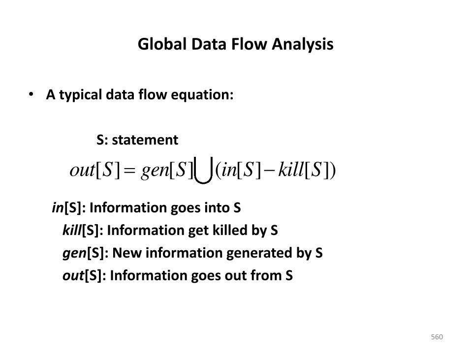
Global Data Flow Analysis

• A typical data flow equation:

S: statement

in[S]: Information goes into S

kill[S]: Information get killed by S

gen[S]: New information generated by S

out[S]: Information goes out from S

560

[ ] [ ] ( [ ] [ ])out S gen S in S kill S

Global Data Flow Analysis

• The notion of gen and kill depends on the desired

information.

• In some cases, in may be defined in terms of out - equation

is solved as analysis traverses in the backward direction.

• Data flow analysis follows control flow graph.

– Equations are set at the level of basic blocks, or even for

a statement

561

Points and Paths

• Point within a basic block:

– A location between two consecutive statements.

– A location before the first statement of the basic block.

– A location after the last statement of the basic block.

• Path: A path from a point p1 to pn is a sequence of points p1, p2, … pn such that for each i : 1 ≤ i ≤ n,

– pi is a point immediately preceding a statement and pi+1 is the point immediately following that statement in the same block, or

– pi is the last point of some block and pi+1 is first point in the successor block.

562

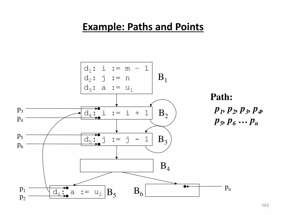
Example: Paths and Points

563

d1: i := m – 1 d2: j := n

d3: a := u1

d4: i := i + 1

d5: j := j - 1

B1

B2

B3

B4

d6: a := u2 B5 B6

pn

p3

p1

p2

p4

p5

p6

Path:

p1, p2, p3, p4,

p5, p6 … pn

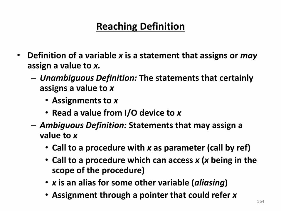
Reaching Definition

• Definition of a variable x is a statement that assigns or may assign a value to x.

– Unambiguous Definition: The statements that certainly assigns a value to x

• Assignments to x

• Read a value from I/O device to x

– Ambiguous Definition: Statements that may assign a value to x

• Call to a procedure with x as parameter (call by ref)

• Call to a procedure which can access x (x being in the scope of the procedure)

• x is an alias for some other variable (aliasing)

• Assignment through a pointer that could refer x 564

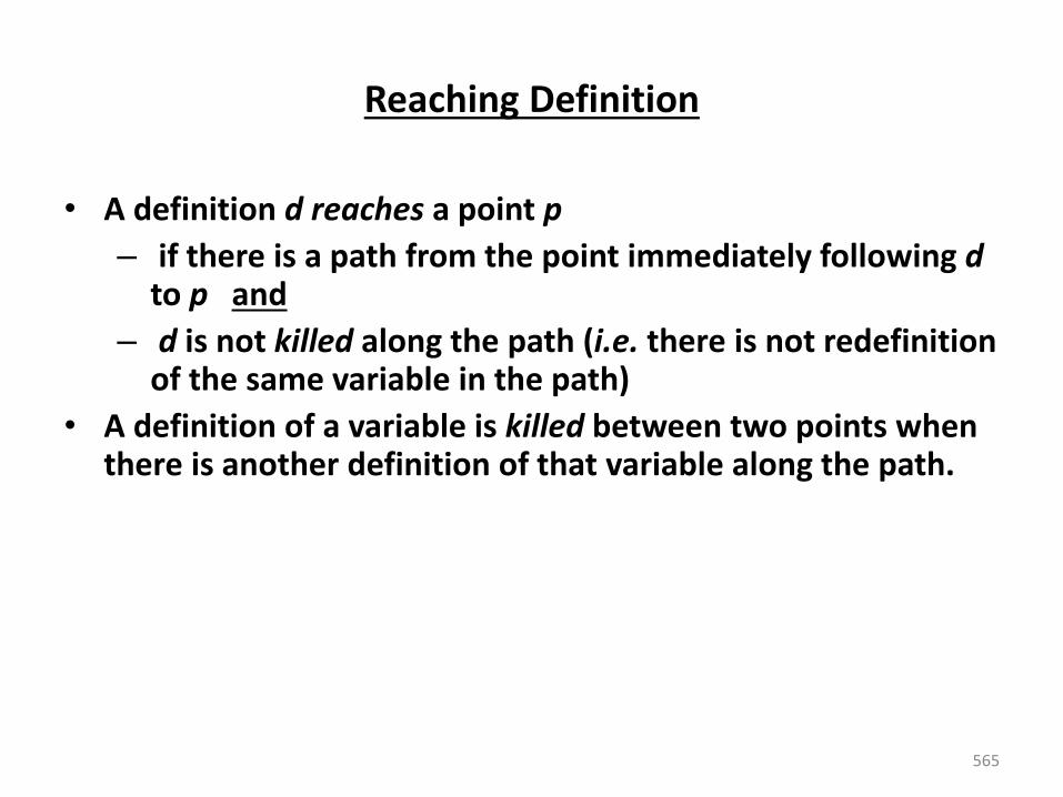
Reaching Definition

• A definition d reaches a point p

– if there is a path from the point immediately following d to p and

– d is not killed along the path (i.e. there is not redefinition of the same variable in the path)

• A definition of a variable is killed between two points when there is another definition of that variable along the path.

565

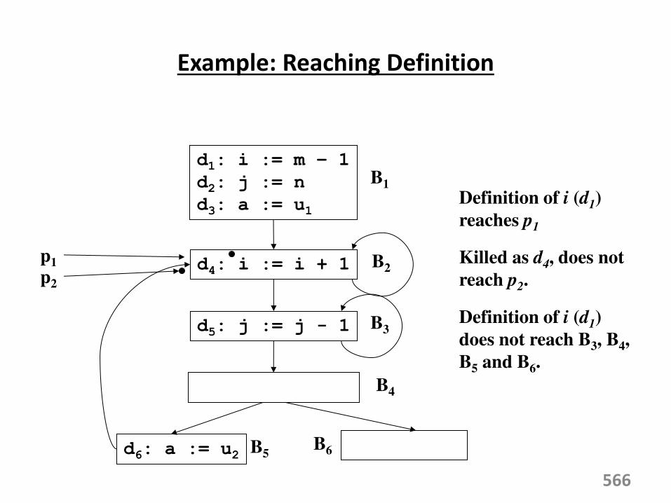
Example: Reaching Definition

566

d1: i := m – 1 d2: j := n d3: a := u1

d4: i := i + 1

d5: j := j - 1

B1

B2

B3

B4

d6: a := u2 B5 B6

p1

p2

Definition of i (d1)

reaches p1

Killed as d4, does not

reach p2.

Definition of i (d1)

does not reach B3, B4,

B5 and B6.

Reaching Definition

• Non-Conservative view: A definition might reach a point even if it might not.

– Only unambiguous definition kills a earlier definition

– All edges of flow graph are assumed to be traversed.

if (a == b) then a = 2

else if (a == b) then a = 4

The defi itio a=4 is ot ea ha le.

Whether each path in a flow graph is taken is an undecidable problem

567

Data Flow analysis of a Structured Program

• Structured programs have well defined loop constructs – the

resultant flow graph is always reducible.

– Without loss of generality we only consider while-do and

if-then-else control constructs

S → id := E│“ ; “

│ if E the “ else “ │ do “ hile E

E → id + id │ id

The non-terminals represent regions.

568

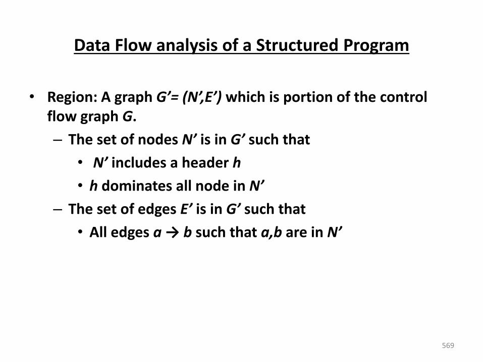
Data Flow analysis of a Structured Program

• Region: A graph G’= N’,E’ which is portion of the control

flow graph G.

– The set of nodes N’ is in G’ such that

• N’ includes a header h

• h dominates all node in N’ – The set of edges E’ is in G’ such that

• All edges a → b such that a,b are in N’

569

Data Flow analysis of a Structured Program

• Region consisting of a statement S:

– Control can flow to only one block outside the region

• Loop is a special case of a region that is strongly connected

and includes all its back edges.

• Dummy blocks with no statements are used as technical

convenience (indicated as open circles)

570

Data Flow analysis of a Structured Program:

Composition of Regions

S → “1 ; S2

571

S1

S2

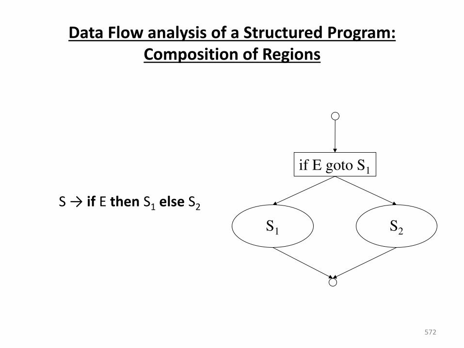
Data Flow analysis of a Structured Program:

Composition of Regions

“ → if E then S1 else S2

572

S1 S2

if E goto S1

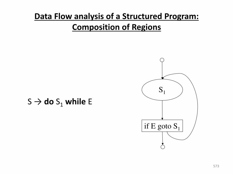
Data Flow analysis of a Structured Program:

Composition of Regions

“ → do S1 while E

573

S1

if E goto S1

Data Flow Equations

• Each region (or NT) has four attributes:

– gen[S]: Set of definitions generated by the block S.

If a definition d is in gen[S], then d reaches the end

of block S.

– kill[S]: Set of definitions killed by block S.

If d is in kill[S], d never reaches the end of block S.

Every path from the beginning of S to the end S

must have a definition for a (where a is defined

by d).

574

Data Flow Equations

– in[S]: The set of definition those are live at the entry point of block S.

– out[S]: The set of definition those are live at the exit point of block S.

• The data flow equations are inductive or syntax directed.

– gen and kill are synthesized attributes.

– in is an inherited attribute.

575

Data Flow Equations

• gen[S] concerns with a single basic block. It is the set of

definitions in S that reaches the end of S.

• In contrast out[S] is the set of definitions (possibly defined

in some other block) live at the end of S considering all

paths through S.

576

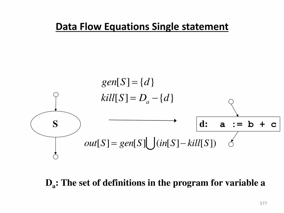
Data Flow Equations Single statement

577

d: a := b + c

[ ] [ ] ( [ ] [ ])out S gen S in S kill S

Da: The set of definitions in the program for variable a

S

[ ] { }

[ ] { }a

gen S d

kill S D d

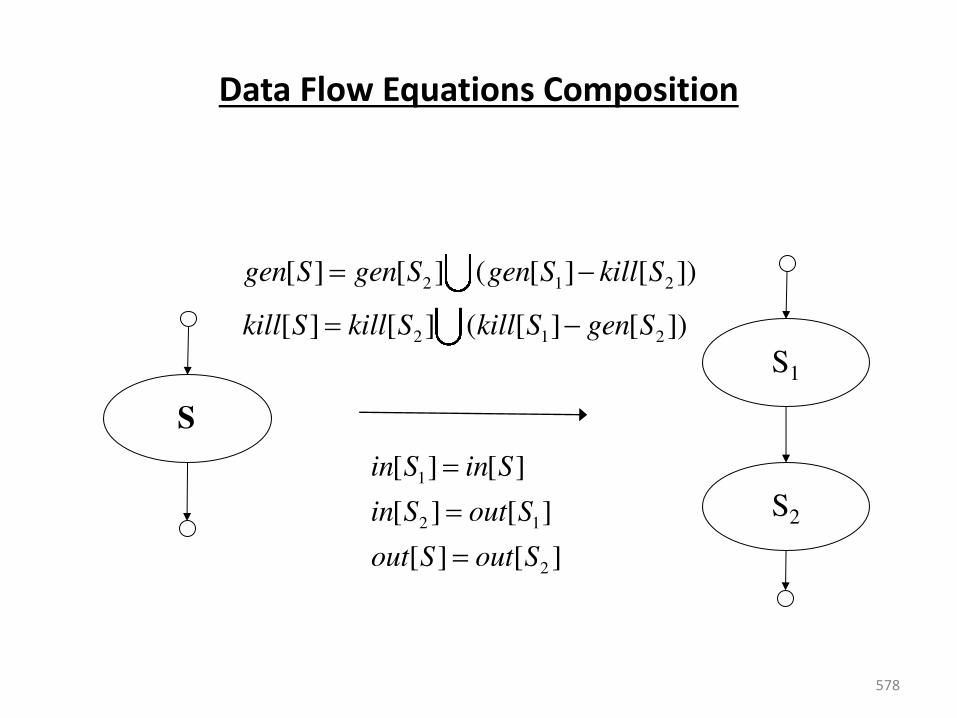
Data Flow Equations Composition

578

S

S1

S2

2 1 2

2 1 2

[ ] [ ] ( [ ] [ ])

[ ] [ ] ( [ ] [ ])

gen S gen S gen S kill S

kill S kill S kill S gen S

1

2 1

2

[ ] [ ]

[ ] [ ]

[ ] [ ]

in S in S

in S out S

out S out S

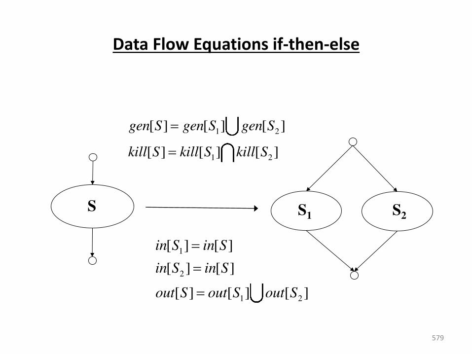
Data Flow Equations if-then-else

579

S1 S2 S

1 2

1 2

[ ] [ ] [ ]

[ ] [ ] [ ]

gen S gen S gen S

kill S kill S kill S

1

2

1 2

[ ] [ ]

[ ] [ ]

[ ] [ ] [ ]

in S in S

in S in S

out S out S out S

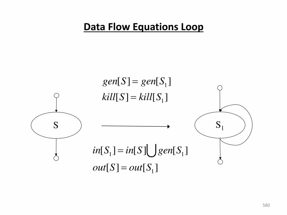
Data Flow Equations Loop

580

S S1

1

1

[ ] [ ]

[ ] [ ]

gen S gen S

kill S kill S

1 1

1

[ ] [ ] [ ]

[ ] [ ]

in S in S gen S

out S out S

Data Flow Analysis

• The attributes are computed for each region. The equations

can be solved in two phases:

– gen and kill can be computed in a single pass of a basic

block.

– in and out are computed iteratively.

• Initial condition for in for the whole program is

• In can be computed top- down

• Finally out is computed

581

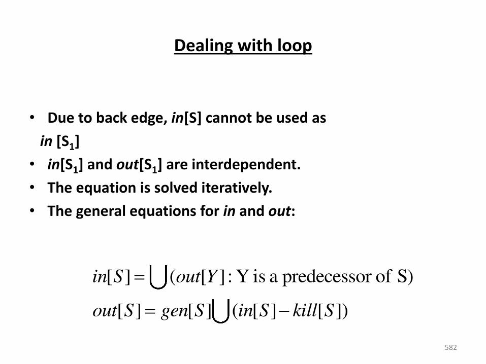
Dealing with loop

• Due to back edge, in[S] cannot be used as

in [S1]

• in[S1] and out[S1] are interdependent.

• The equation is solved iteratively.

• The general equations for in and out:

582

[ ] ( [ ] : Y is a predecessor of S)

[ ] [ ] ( [ ] [ ])

in S out Y

out S gen S in S kill S

Reaching definitions

• What is safe?

– To assume that a definition reaches a point even if it

turns out not to.

– The computed set of definitions reaching a point p

will be a superset of the actual set of definitions

reaching p

– Goal : make the set of reaching definitions as small

as possible (i.e. as close to the actual set as possible)

583

Reaching definitions

• How are the gen and kill sets defined?

– gen[B] = {definitions that appear in B and reach the

end of B}

– kill[B] = {all definitions that never reach the end of B}

• What is the direction of the analysis?

– forward

– out[B] = gen[B] (in[B] - kill[B])

584

Reaching definitions

• What is the confluence operator?

– union

– in[B] = out[P], over the predecessors P of B

• How do we initialize?

– start small

• Why? Because we want the resulting set to be as

small as possible

– for each block B initialize out[B] = gen[B]

585

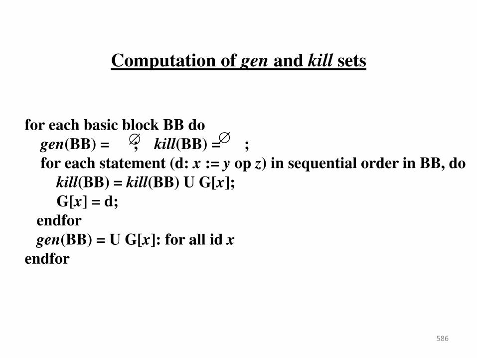
Computation of gen and kill sets

586

for each basic block BB do

gen(BB) = ; kill(BB) = ;

for each statement (d: x := y op z) in sequential order in BB, do

kill(BB) = kill(BB) U G[x];

G[x] = d;

endfor

gen(BB) = U G[x]: for all id x

endfor

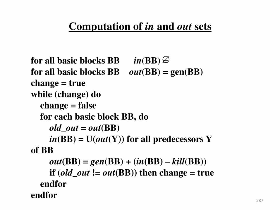
Computation of in and out sets

587

for all basic blocks BB in(BB) =

for all basic blocks BB out(BB) = gen(BB)

change = true

while (change) do

change = false

for each basic block BB, do

old_out = out(BB)

in(BB) = U(out(Y)) for all predecessors Y

of BB

out(BB) = gen(BB) + (in(BB) – kill(BB))

if (old_out != out(BB)) then change = true

endfor

endfor

Live Variable (Liveness) Analysis

• Liveness: For each point p in a program and each variable y, determine whether y can be used before being redefined, starting at p.

• Attributes

– use = set of variable used in the BB prior to its definition

– def = set of variables defined in BB prior to any use of the variable

– in = set of variables that are live at the entry point of a BB

– out = set of variables that are live at the exit point of a BB

588

Live Variable (Liveness) Analysis

• Data flow equations:

– 1st Equation: a var is live, coming in the block, if either • it is used before redefinition in B or • it is live coming out of B and is not redefined in B

– 2nd Equation: a var is live coming out of B, iff it is live coming in to one of its successors.

589

( )

[ ] [ ] ( [ ] [ ])

[ ] [ ]S succ B

in B use B out B def B

out B in S

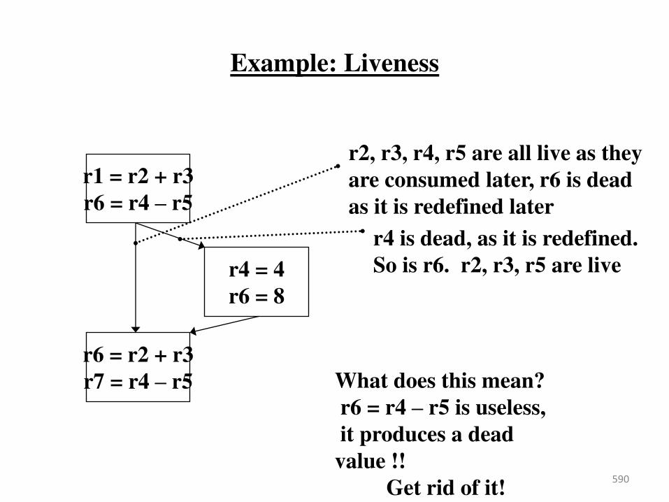
Example: Liveness

590

r1 = r2 + r3

r6 = r4 – r5

r4 = 4

r6 = 8

r6 = r2 + r3

r7 = r4 – r5

r2, r3, r4, r5 are all live as they

are consumed later, r6 is dead

as it is redefined later

r4 is dead, as it is redefined.

So is r6. r2, r3, r5 are live

What does this mean?

r6 = r4 – r5 is useless,

it produces a dead

value !!

Get rid of it!

Computation of use and def sets

591

for each basic block BB do

def(BB) = ; use(BB) = ;

for each statement (x := y op z) in sequential order, do

for each operand y, do

if (y not in def(BB))

use(BB) = use(BB) U {y};

endfor

def(BB) = def(BB) U {x};

endfor

def is the union of all the LHS’s

use is all the ids used before defined

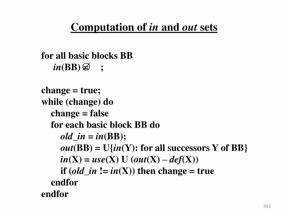
Computation of in and out sets

592

for all basic blocks BB

in(BB) = ;

change = true;

while (change) do

change = false

for each basic block BB do

old_in = in(BB);

out(BB) = U{in(Y): for all successors Y of BB}

in(X) = use(X) U (out(X) – def(X))

if (old_in != in(X)) then change = true

endfor

endfor

DU/UD Chains

• Convenient way to access/use reaching definition

information.

• Def-Use chains (DU chains)

– Given a def, what are all the possible consumers of the

definition produced

• Use-Def chains (UD chains)

– Given a use, what are all the possible producers of the

definition consumed

593

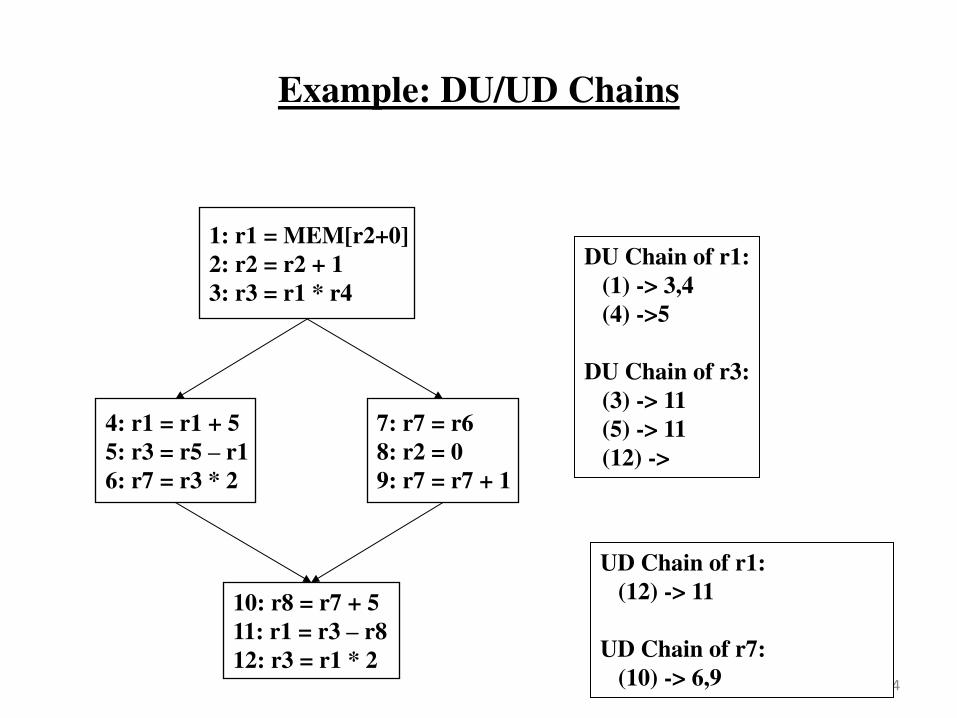
Example: DU/UD Chains

594

1: r1 = MEM[r2+0]

2: r2 = r2 + 1

3: r3 = r1 * r4

4: r1 = r1 + 5

5: r3 = r5 – r1

6: r7 = r3 * 2

7: r7 = r6

8: r2 = 0

9: r7 = r7 + 1

10: r8 = r7 + 5

11: r1 = r3 – r8

12: r3 = r1 * 2

DU Chain of r1:

(1) -> 3,4

(4) ->5

DU Chain of r3:

(3) -> 11

(5) -> 11

(12) ->

UD Chain of r1:

(12) -> 11

UD Chain of r7:

(10) -> 6,9

Some-things to Think About

• Liveness and Reaching definitions are basically the same thing!

– All dataflow is basically the same with a few parameters

• Meaning of gen/kill (use/def)

• Backward / Forward

• All paths / some paths (must/may)

– So far, we have looked at may analysis algorithms

– How do you adjust to do must algorithms?

• Dataflow can be slow

– How to implement it efficiently?

– How to represent the info?

595

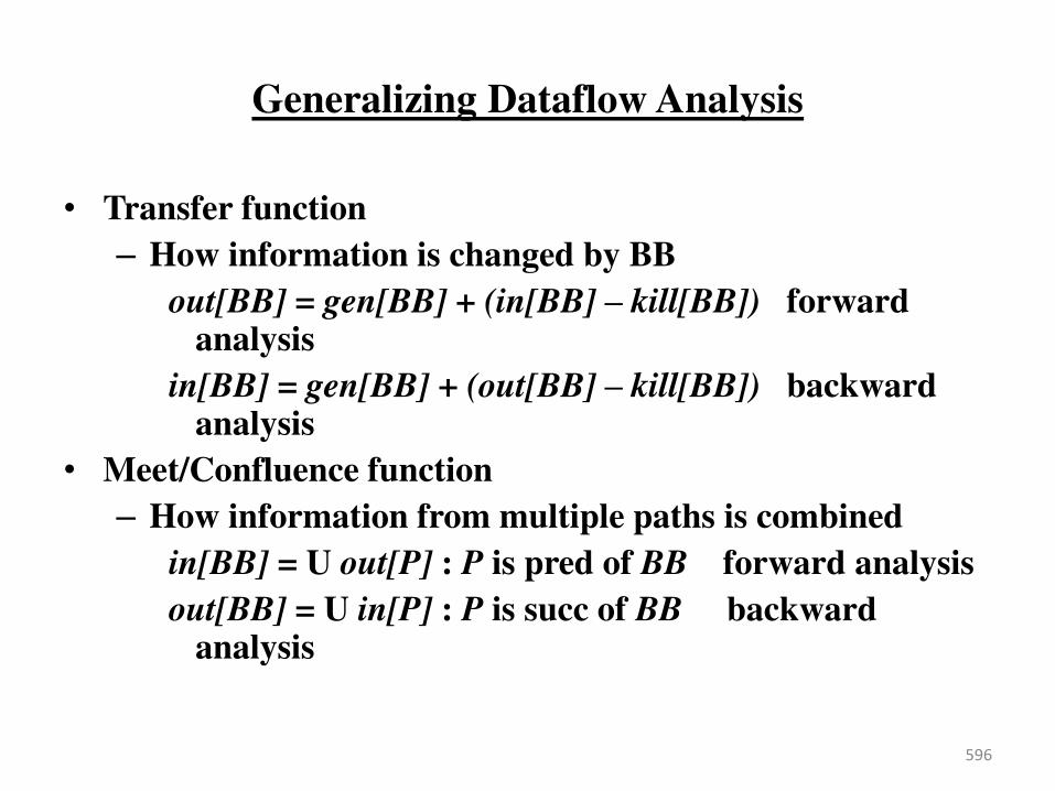
Generalizing Dataflow Analysis

• Transfer function

– How information is changed by BB

out[BB] = gen[BB] + (in[BB] – kill[BB]) forward analysis

in[BB] = gen[BB] + (out[BB] – kill[BB]) backward analysis

• Meet/Confluence function

– How information from multiple paths is combined

in[BB] = U out[P] : P is pred of BB forward analysis

out[BB] = U in[P] : P is succ of BB backward analysis

596

Generalized Dataflow Algorithm

change = true;

while (change)

change = false;

for each BB

apply meet function

apply transfer function

if any changes change = true;

597

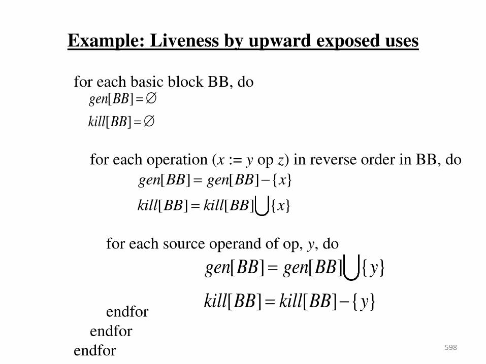
Example: Liveness by upward exposed uses

598

for each basic block BB, do

for each operation (x := y op z) in reverse order in BB, do

for each source operand of op, y, do

endfor

endfor

endfor

[ ]

[ ]

gen BB

kill BB

[ ] [ ] { }

[ ] [ ] { }

gen BB gen BB x

kill BB kill BB x

[ ] [ ] { }

[ ] [ ] { }

gen BB gen BB y

kill BB kill BB y

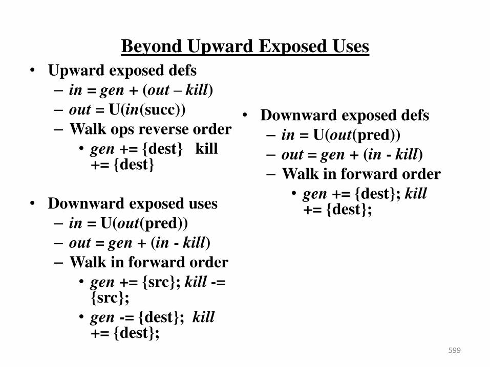
Beyond Upward Exposed Uses

• Upward exposed defs

– in = gen + (out – kill)

– out = U(in(succ))

– Walk ops reverse order

• gen += {dest} kill += {dest}

• Downward exposed uses

– in = U(out(pred))

– out = gen + (in - kill)

– Walk in forward order

• gen += {src}; kill -= {src};

• gen -= {dest}; kill += {dest};

• Downward exposed defs

– in = U(out(pred))

– out = gen + (in - kill)

– Walk in forward order

• gen += {dest}; kill += {dest};

599

All Path Problem

• Up to this point

– Any path problems (maybe relations)

• Definition reaches along some path

• Some sequence of branches in which def reaches

• Lots of defs of the same variable may reach a point

– Use of Union operator in meet function

• All-path: Definition guaranteed to reach

– Regardless of sequence of branches taken, def reaches

– Can always count on this

– Only 1 def can be guaranteed to reach

– Availability (as opposed to reaching)

• Available definitions

• Available expressions (could also have reaching expressions, but not that useful)

600

Reaching vs Available Definitions

601

1: r1 = r2 + r3

2: r6 = r4 – r5

3: r4 = 4

4: r6 = 8

5: r6 = r2 + r3

6: r7 = r4 – r5 1,2,3,4 reach

1 available

1,2 reach

1,2 available

1,3,4 reach

1,3,4 available

1,2 reach

1,2 available

Available Definition Analysis (Adefs)

• A definition d is available at a point p if along all paths from d to p, d is not killed

• Remember, a definition of a variable is killed between 2 points when there is another definition of that variable along the path

– r1 = r2 + r3 kills previous definitions of r1

• Algorithm:

– Forward dataflow analysis as propagation occurs from defs downwards

– Use the Intersect function as the meet operator to guarantee the all-path requirement

– gen/kill/in/out similar to reaching defs

• Initialization of in/out is the tricky part

602

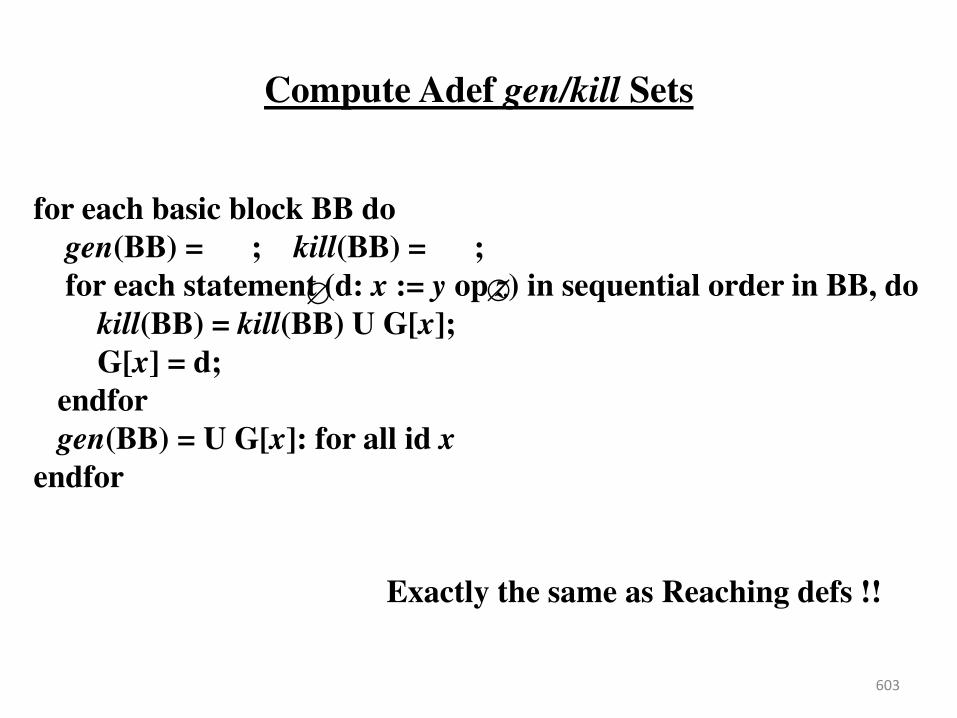
Compute Adef gen/kill Sets

603

Exactly the same as Reaching defs !!

for each basic block BB do

gen(BB) = ; kill(BB) = ;

for each statement (d: x := y op z) in sequential order in BB, do

kill(BB) = kill(BB) U G[x];

G[x] = d;

endfor

gen(BB) = U G[x]: for all id x

endfor

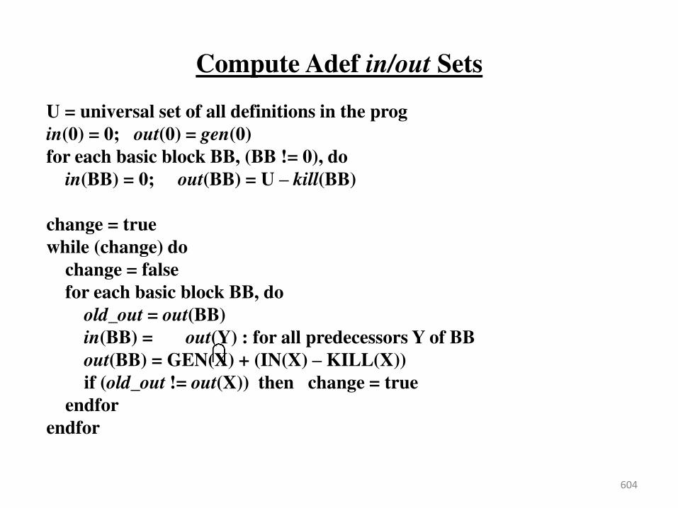
Compute Adef in/out Sets

604

U = universal set of all definitions in the prog

in(0) = 0; out(0) = gen(0)

for each basic block BB, (BB != 0), do

in(BB) = 0; out(BB) = U – kill(BB)

change = true

while (change) do

change = false

for each basic block BB, do

old_out = out(BB)

in(BB) = out(Y) : for all predecessors Y of BB

out(BB) = GEN(X) + (IN(X) – KILL(X))

if (old_out != out(X)) then change = true

endfor

endfor

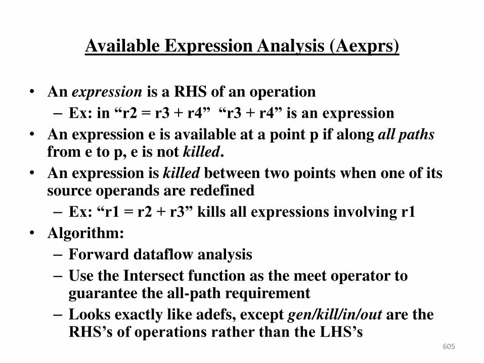
Available Expression Analysis (Aexprs)

• An expression is a RHS of an operation

– Ex: in “rβ = rγ + r4” “rγ + r4” is an expression

• An expression e is available at a point p if along all paths from e to p, e is not killed.

• An expression is killed between two points when one of its source operands are redefined

– Ex: “r1 = rβ + rγ” kills all expressions involving r1

• Algorithm:

– Forward dataflow analysis

– Use the Intersect function as the meet operator to guarantee the all-path requirement

– Looks exactly like adefs, except gen/kill/in/out are the RHS’s of operations rather than the LHS’s

605

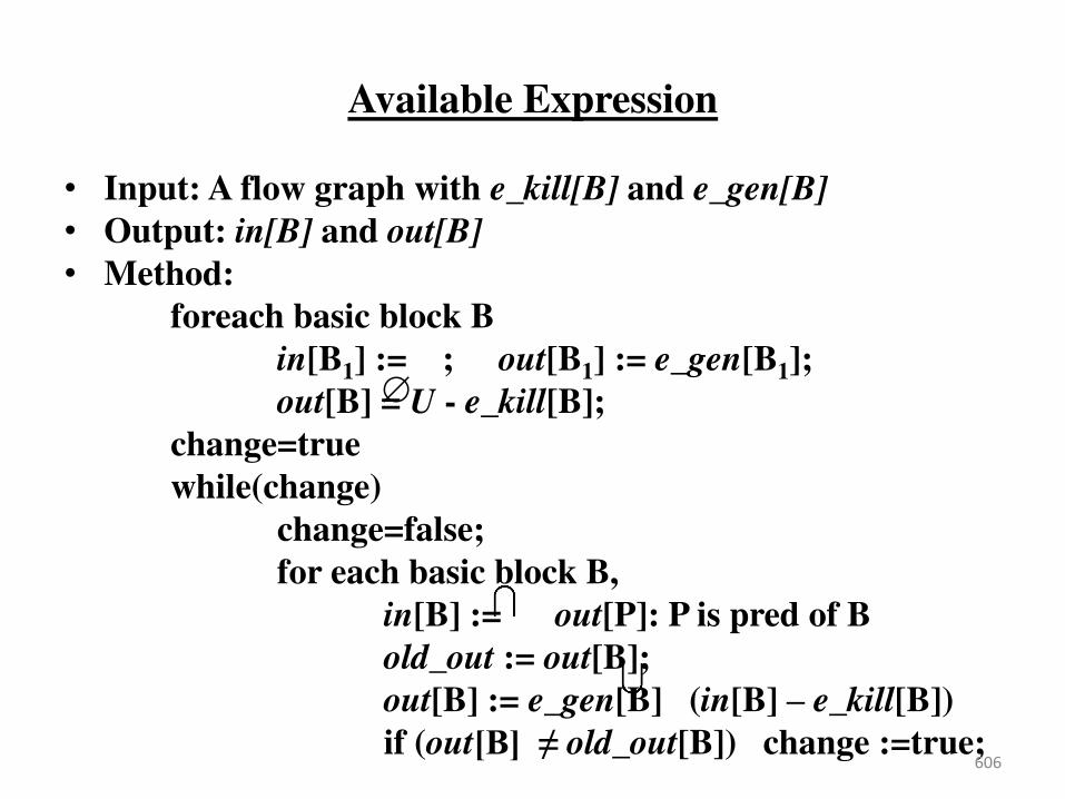
Available Expression

• Input: A flow graph with e_kill[B] and e_gen[B]

• Output: in[B] and out[B]

• Method:

foreach basic block B

in[B1] := ; out[B1] := e_gen[B1];

out[B] = U - e_kill[B];

change=true

while(change)

change=false;

for each basic block B,

in[B] := out[P]: P is pred of B

old_out := out[B];

out[B] := e_gen[B] (in[B] – e_kill[B])

if (out[B] ≠ old_out[B]) change :=true;

606

Efficient Calculation of Dataflow

• Order in which the basic blocks are visited is important (faster convergence)

• Forward analysis – DFS order

– Visit a node only when all its predecessors have been visited

• Backward analysis – Post DFS order

– Visit a node only when all of its successors have been visited

607

Representing Dataflow Information

• Requirements – Efficiency!

– Large amount of information to store

– Fast access/manipulation

• Bitvectors

– General strategy used by most compilers

– Bit positions represent defs (rdefs)

– Efficient set operations: union/intersect/isone

– Used for gen, kill, in, out for each BB

608

Optimization using Dataflow

• Classes of optimization

1. Classical (machine independent)

• Reducing operation count (redundancy elimination)

• Simplifying operations

2. Machine specific

• Peephole optimizations

• Take advantage of specialized hardware features

3. Instruction Level Parallelism (ILP) enhancing

• Increasing parallelism

• Possibly increase instructions

609

Types of Classical Optimizations

• Operation-level – One operation in isolation

– Constant folding, strength reduction

– Dead code elimination (global, but 1 op at a time)

• Local – Pairs of operations in same BB

– May or may not use dataflow analysis

• Global – Again pairs of operations

– Pairs of operations in different BBs

• Loop – Body of a loop

610

Constant Folding

• Simplify operation based on values of target operand

– Constant propagation creates opportunities for this

• All constant operands

– Evaluate the op, replace with a move

• r1 = 3 * 4 r1 = 12

• r1 = 3 / 0 ??? Don’t evaluate excepting ops !, what about FP?

– Evaluate conditional branch, replace with BRU or noop

• if (1 < 2) goto BB2 goto BB2

• if (1 > 2) goto BB2 convert to a noop Dead code

• Algebraic identities

– r1 = r2 + 0, r2 – 0, r2 | 0, r2 ^ 0, r2 << 0, r2 >> 0 r1 = r2

– r1 = 0 * r2, 0 / r2, 0 & r2 r1 = 0

– r1 = r2 * 1, r2 / 1 r1 = r2 611

Strength Reduction

• Replace expensive ops with cheaper ones

– Constant propagation creates opportunities for this

• Power of 2 constants

– Mult by power of 2: r1 = r2 * 8 r1 = r2 << 3

– Div by power of 2: r1 = r2 / 4 r1 = r2 >> 2

– Rem by power of 2: r1 = r2 % 16 r1 = r2 & 15

• More exotic

– Replace multiply by constant by sequence of shift and adds/subs

• r1 = r2 * 6

– r100 = r2 << 2; r101 = r2 << 1; r1 = r100 + r101

• r1 = r2 * 7

– r100 = r2 << 3; r1 = r100 – r2 612

Dead Code Elimination

• Remove statement d: x := y op z whose result is never

consumed.

• Rules:

– DU chain for d is empty

– y and z are not live at d

613

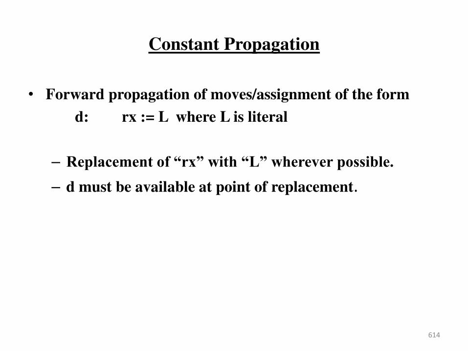
Constant Propagation

• Forward propagation of moves/assignment of the form

d: rx := L where L is literal

– Replacement of “rx” with “L” wherever possible. – d must be available at point of replacement.

614

Forward Copy Propagation

• Fo a d p opagatio of ‘H“ of assig e t o o s.

– Reduce chain of dependency

– Possibly create dead code

615

r1 := r2 . . . r4 := r1 + 1

r1 := r2 . . . r4 := r2 + 1

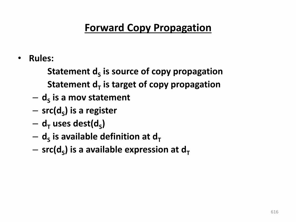
Forward Copy Propagation

• Rules:

Statement dS is source of copy propagation

Statement dT is target of copy propagation

– dS is a mov statement

– src(dS) is a register

– dT uses dest(dS)

– dS is available definition at dT

– src(dS) is a available expression at dT

616

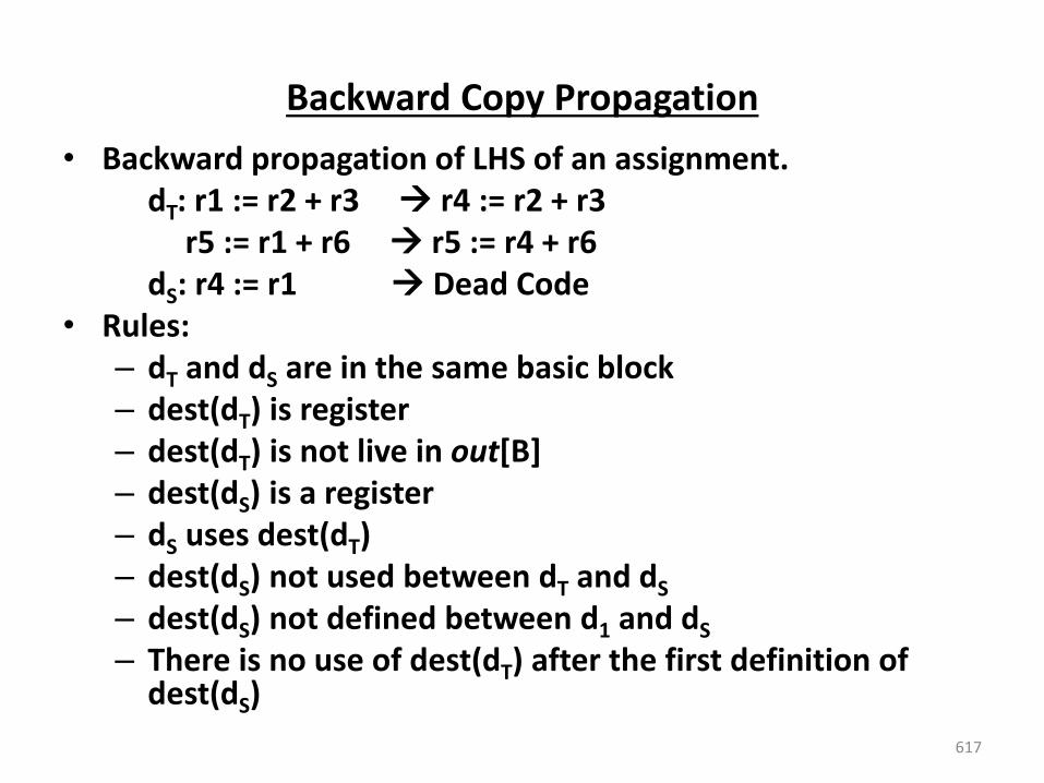
Backward Copy Propagation

• Backward propagation of LHS of an assignment.

dT: r1 := r2 + r3 r4 := r2 + r3

r5 := r1 + r6 r5 := r4 + r6

dS: r4 := r1 Dead Code

• Rules:

– dT and dS are in the same basic block

– dest(dT) is register

– dest(dT) is not live in out[B]

– dest(dS) is a register

– dS uses dest(dT)

– dest(dS) not used between dT and dS

– dest(dS) not defined between d1 and dS

– There is no use of dest(dT) after the first definition of dest(dS)

617

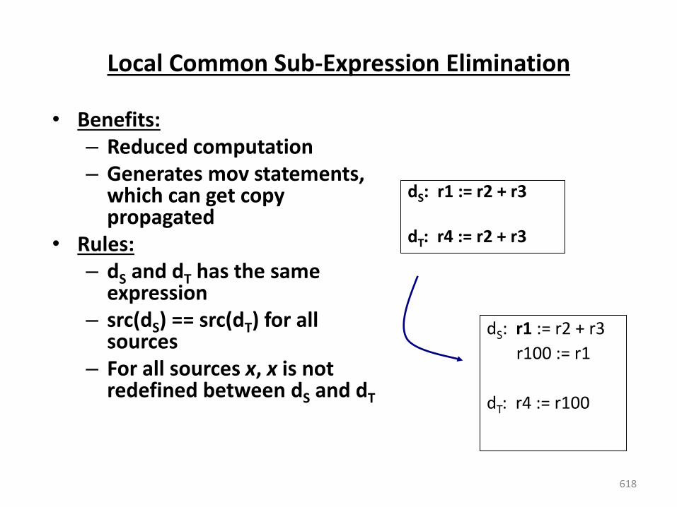
Local Common Sub-Expression Elimination

• Benefits:

– Reduced computation

– Generates mov statements, which can get copy propagated

• Rules:

– dS and dT has the same expression

– src(dS) == src(dT) for all sources

– For all sources x, x is not redefined between dS and dT

dS: r1 := r2 + r3

dT: r4 := r2 + r3

618

dS: r1 := r2 + r3

r100 := r1

dT: r4 := r100

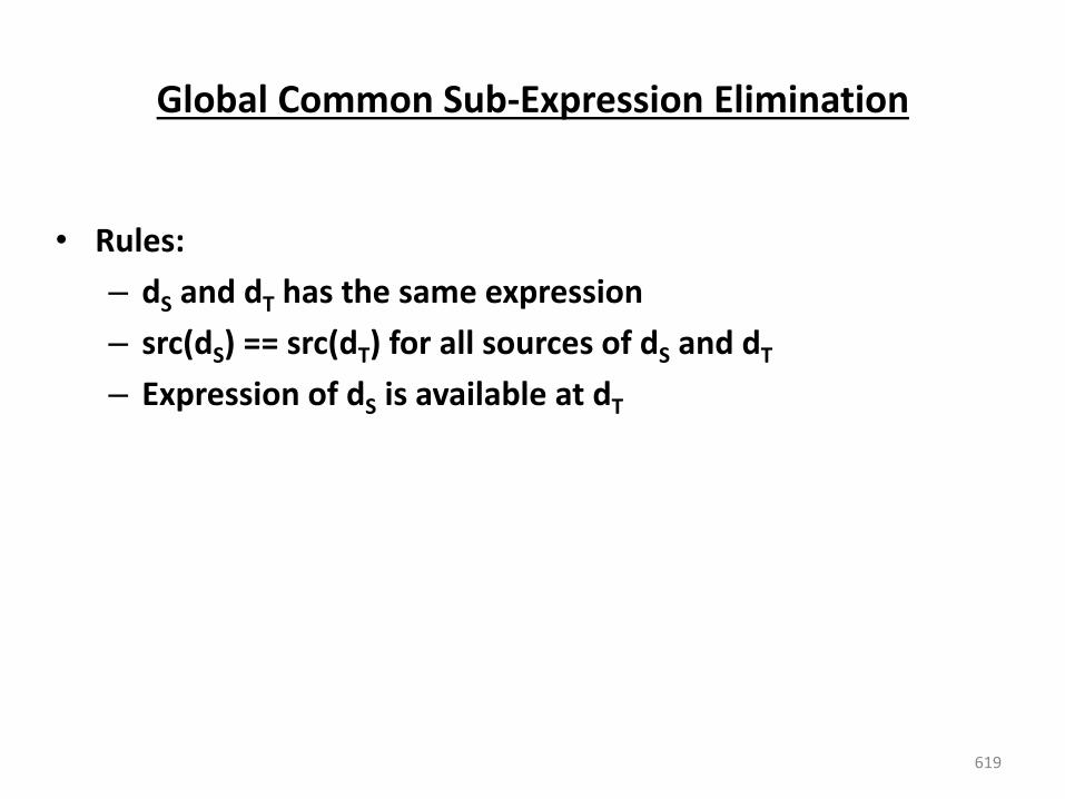
Global Common Sub-Expression Elimination

• Rules:

– dS and dT has the same expression

– src(dS) == src(dT) for all sources of dS and dT

– Expression of dS is available at dT

619

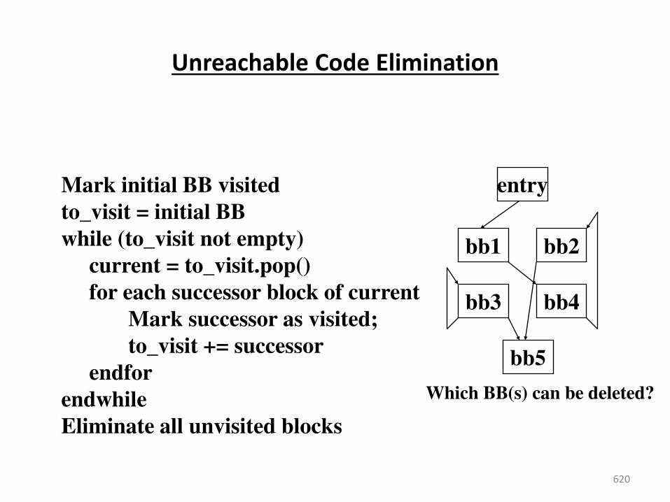
Unreachable Code Elimination

620

Mark initial BB visited

to_visit = initial BB

while (to_visit not empty)

current = to_visit.pop()

for each successor block of current

Mark successor as visited;

to_visit += successor

endfor

endwhile

Eliminate all unvisited blocks

entry

bb1 bb2

bb3 bb4

bb5

Which BB(s) can be deleted?

Unit-5

OBJECT CODE GENERATION

CODE GENERATION

• The final phase in our compiler model is the code generator.

It takes as input an intermediate representation of the

source program and produces as output an equivalent target

program.

• The requirements traditionally imposed on a code generator

are severe. The output code must be correct and of high

quality, meaning that it should make effective use of the

resources of the target machine. Moreover, the code

generator itself should run efficiently.

ISSUES IN THE DESIGN OF A CODE GENERATOR

While the details are dependent on the target language and

the operating system, issues such as memory management,

instruction selection, register allocation, and evaluation order

are inherent in almost all code generation problems .

INPUT TO THE CODE GENERATOR

• The input to the code generator consists of the

intermediate representation of the source program

produced by the front end, together with information in the

symbol table that is used to determine the run time

addresses of the data objects denoted by the names in the

intermediate representation.

• There are several choices for the intermediate

language, including: linear representations such as postfix

notation, three address representations such as quadruples,

virtual machine representations such as syntax trees and

dags.

INPUT TO THE CODE GENERATOR

• We assume that prior to code generation the front end has scanned, parsed, and translated the source program into a reasonably detailed intermediate representation, so the values of names appearing in the intermediate language can be represented by quantities that the target machine can directly manipulate (bits, integers, reals, pointers, etc.). We also assume that the necessary type checking has take place, so type conversion operators have been inserted wherever necessary and obvious semantic errors (e.g., attempting to index an array by a floating point number) have already been detected. The code generation phase can therefore proceed on the assumption that its input is free of errors. In some compilers, this kind of semantic checking is done together with code generation .

TARGET PROGRAMS

• The output of the code generator is the target program. The

output may take on a variety of forms: absolute machine

language, relocatable machine language, or assembly

language.

• Producing an absolute machine language

program as output has the advantage that it can be placed in

a location in memory and immediately executed. A small

program can be compiled and executed quickly. A number of

stude t-jo o pile s, su h as WATFIV a d PL/C, p odu e absolute code.

TARGET PROGRAMS

• Producing a relocatable machine language program as output allows subprograms to be compiled separately. A set of relocatable object modules can be linked together and loaded for execution by a linking loader. Although we must pay the added expense of linking and loading if we produce relocatable object modules, we gain a great deal of flexibility in being able to compile subroutines separately and to call other previously compiled programs from an object module. If the target machine does not handle relocation automatically, the compiler must provide explicit relocation information to the loader to link the separately compiled program segments

TARGET PROGRAMS

• Producing an assembly language program as output makes

the process of code generation somewhat easier .We can

generate symbolic instructions and use the macro facilities

of the assembler to help generate code .The price paid is the

assembly step after code generation.

• Because producing assembly code does not duplicate the

entire task of the assembler, this choice is another

reasonable alternative, especially for a machine with a small

memory, where a compiler must uses several passes.

MEMORY MANAGEMENT

Mapping names in the source program to addresses of data

objects in run time memory is done cooperatively by the

front end and the code generator. We assume that a name in

a three-address statement refers to a symbol table entry for

the name.

MEMORY MANAGEMENT If machine code is being generated, labels in three address

statements have to be converted to addresses of i st u tio s. This p o ess is a alogous to the a k pat hi g . “uppose that la els efe to uad uple u e s in a quadruple array. As we scan each quadruple in turn we can deduce the location of the first machine instruction generated for that quadruple, simply by maintaining a count of the number of words used for the instructions generated so far. This count can be kept in the quadruple array (in an extra field), so if a reference such as j: goto i is encountered, and i is less than j, the current quadruple number, we may simply generate a jump instruction with the target address equal to the machine location of the first instruction in the code for quadruple i. If, however, the jump is forward, so i exceeds j, we must store on a list for quadruple i the location of the first machine instruction generated for quadruple j. Then we process quadruple i, we fill in the proper machine location for all instructions that are forward jumps to i.

INSTRUCTION SELECTION

• The nature of the instruction set of the target machine

determines the difficulty of instruction selection. The

uniformity and completeness of the instruction set are

important factors. If the target machine does not support

each data type in a uniform manner, then each exception to

the general rule requires special handling.

• Instruction speeds and machine idioms are other important

factors. If we do not care about the efficiency of the target

program, instruction selection is straightforward. For each

type of three- address statement we can design a code

skeleton that outlines the target code to be generated for

that construct.

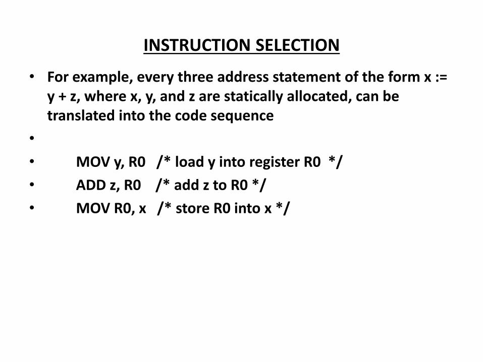
INSTRUCTION SELECTION

• For example, every three address statement of the form x :=

y + z, where x, y, and z are statically allocated, can be

translated into the code sequence

•

• MOV y, R0 /* load y into register R0 */

• ADD z, R0 /* add z to R0 */

• MOV R0, x /* store R0 into x */

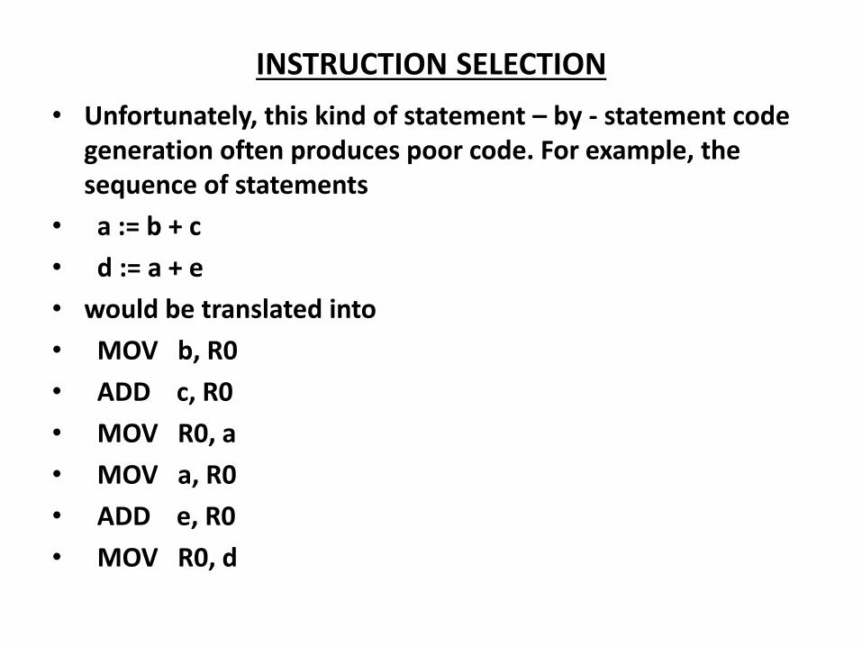
INSTRUCTION SELECTION

• Unfortunately, this kind of statement – by - statement code

generation often produces poor code. For example, the

sequence of statements

• a := b + c

• d := a + e

• would be translated into

• MOV b, R0

• ADD c, R0

• MOV R0, a

• MOV a, R0

• ADD e, R0

• MOV R0, d

INSTRUCTION SELECTION

• Here the fourth statement is redundant, and so is the third if

a is ot su se ue tl used. • The quality of the generated code is determined

by its speed and size.

• A target machine with a rich instruction set may provide

several ways of implementing a given operation. Since the

cost differences between different implementations may be

significant, a naive translation of the intermediate code may

lead to correct, but unacceptably inefficient target code.

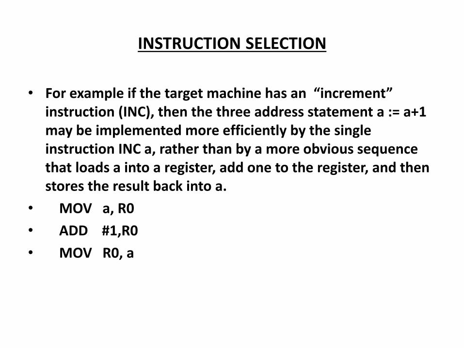
INSTRUCTION SELECTION

• Fo e a ple if the ta get a hi e has a i e e t instruction (INC), then the three address statement a := a+1

may be implemented more efficiently by the single

instruction INC a, rather than by a more obvious sequence

that loads a into a register, add one to the register, and then

stores the result back into a.

• MOV a, R0

• ADD #1,R0

• MOV R0, a

INSTRUCTION SELECTION

Instruction speeds are needed to design good code

sequence but unfortunately, accurate timing information is

often difficult to obtain. Deciding which machine code

sequence is best for a given three address construct may

also require knowledge about the context in which that

construct appears.

REGISTER ALLOCATION

Instructions involving register operands are usually shorter

and faster than those involving operands in memory.

Therefore, efficient utilization of register is particularly

important in generating good code. The use of registers is

often subdivided into two subproblems:

REGISTER ALLOCATION

1. During register allocation, we select the set of variables

that will reside in registers at a point in the program.

2. During a subsequent register assignment phase, we pick

the specific register that a variable will reside in.

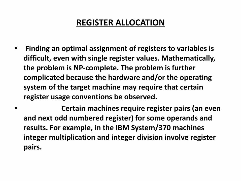
REGISTER ALLOCATION

• Finding an optimal assignment of registers to variables is

difficult, even with single register values. Mathematically,

the problem is NP-complete. The problem is further

complicated because the hardware and/or the operating

system of the target machine may require that certain

register usage conventions be observed.

• Certain machines require register pairs (an even

and next odd numbered register) for some operands and

results. For example, in the IBM System/370 machines

integer multiplication and integer division involve register

pairs.

REGISTER ALLOCATION

• The multiplication instruction is of the form

• M x, y

• where x, is the multiplicand, is the even register of an

even/odd register pair.

• The multiplicand value is taken from the odd register

pair. The multiplier y is a single register. The product

occupies the entire even/odd register pair.

• The division instruction is of the form

• D x, y

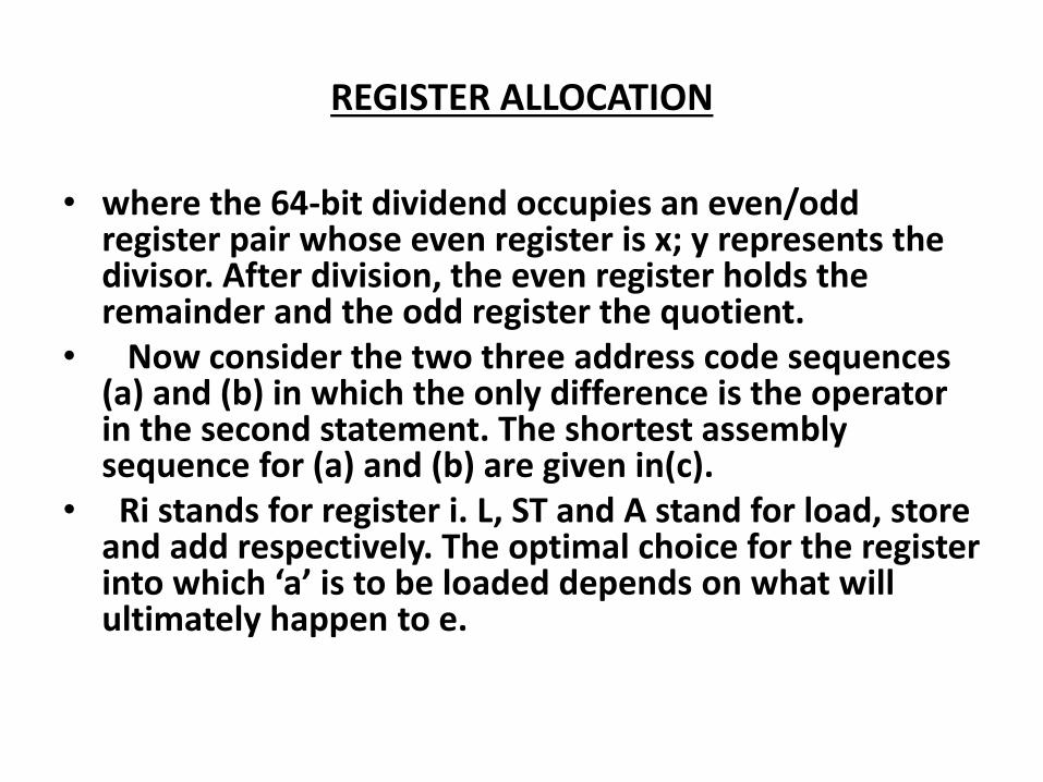
REGISTER ALLOCATION

• where the 64-bit dividend occupies an even/odd register pair whose even register is x; y represents the divisor. After division, the even register holds the remainder and the odd register the quotient.

• Now consider the two three address code sequences (a) and (b) in which the only difference is the operator in the second statement. The shortest assembly sequence for (a) and (b) are given in(c).

• Ri stands for register i. L, ST and A stand for load, store and add respectively. The optimal choice for the register i to hi h a is to e loaded depe ds o hat ill ultimately happen to e.

REGISTER ALLOCATION

• t := a + b t := a + b

• t := t * c t := t + c

• t := t / d t := t / d

(a) (b)

• Two three address code sequences

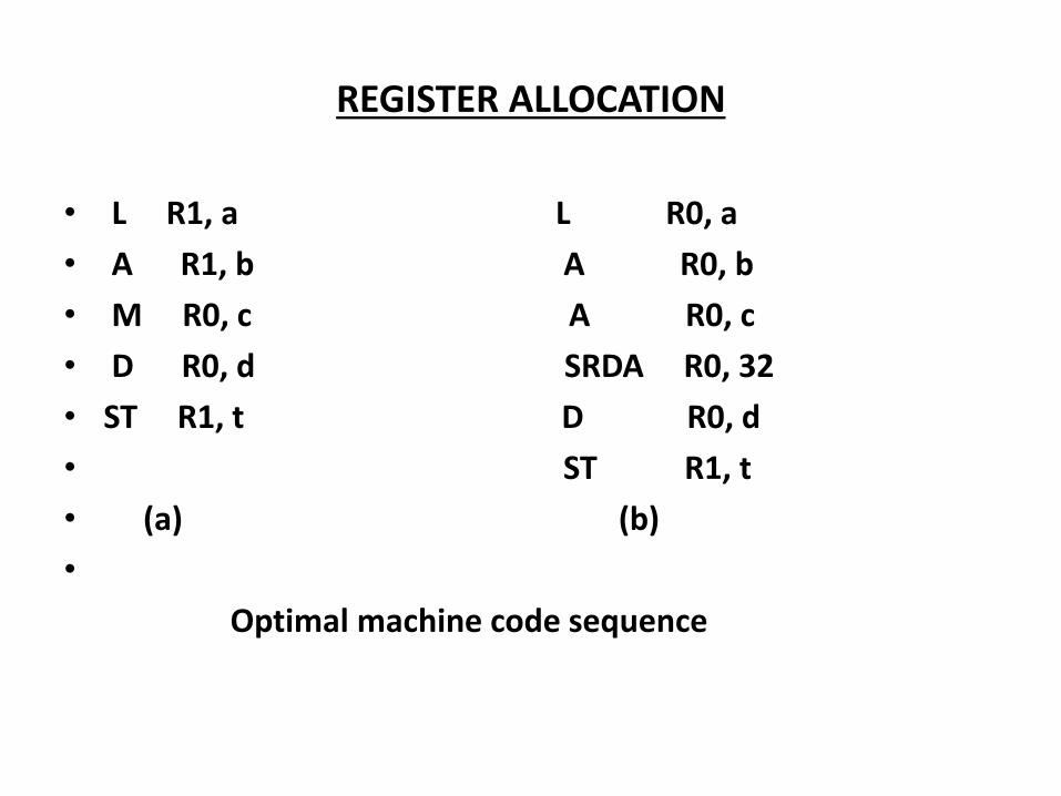
REGISTER ALLOCATION

• L R1, a L R0, a

• A R1, b A R0, b

• M R0, c A R0, c

• D R0, d SRDA R0, 32

• ST R1, t D R0, d

• ST R1, t

• (a) (b)

•

Optimal machine code sequence

CHOICE OF EVALUATION ORDER

• The order in which computations are performed can affect

the efficiency of the target code. Some computation orders

require fewer registers to hold intermediate results than

others. Picking a best order is another difficult, NP-complete

problem. Initially, we shall avoid the problem by generating

code for the three -address statements in the order in which

they have been produced by the intermediate code

generator.

APPROCHES TO CODE GENERATION

• The most important criterion for a code generator is

that it produce correct code. Correctness takes on

special significance because of the number of

special cases that code generator must face. Given

the premium on correctness, designing a code

generator so it can be easily implemented, tested,

and maintained is an important design goal.